HP 49GPLUS Graphing Calculator User Manual

hp 49g+ graphing calculator

user’s manual

Edition 2 HP part number F2228-90001

Notice

THIS MANUAL AND ANY EXAMPLES CONTAINED HEREIN ARE PROVIDED “AS IS” AND ARE SUBJECT TO CHANGE WITHOUT NOTICE. HEWLETT-PACKARD COMPANY MAKES NO WARRANTY OF ANY KIND WITH REGARD TO THIS MANUAL, INCLUDING, BUT NOT LIMITED TO, THE IMPLIED WARRANTIES OF MERCHANTABILITY, NON-INFRINGEMENT AND FITNESS FOR A PARTICULAR PURPOSE.

HEWLETT-PACKARD CO. SHALL NOT BE LIABLE FOR ANY ERRORS OR FOR INCIDENTAL OR CONSEQUENTIAL DAMAGES IN CONNECTION WITH THE FURNISHING, PERFORMANCE, OR USE OF THIS MANUAL OR THE EXAMPLES CONTAINED HEREIN.

© Copyright 2003 Hewlett-Packard Development Company, L.P. Reproduction, adaptation, or translation of this manual is prohibited without prior written permission of Hewlett-Packard Company, except as allowed under the copyright laws.

Hewlett-Packard Company 4995 Murphy Canyon Rd, Suite 301 San Diego,CA 92123

Printing History

Edition 2 December 2003

Preface

You have in your hands a compact symbolic and numerical computer that will facilitate calculation and mathematical analysis of problems in a variety of disciplines, from elementary mathematics to advanced engineering and science subjects.

This manual contains examples that illustrate the use of the basic calculator functions and operations. The chapters in this user’s manual are organized by subject in order of difficulty: from the setting of calculator modes, to real and complex number calculations, operations with lists, vectors, and matrices, graphics, calculus applications, vector analysis, differential equations, probability and statistics.

For symbolic operations the calculator includes a powerful Computer Algebraic System (CAS), which lets you select different modes of operation, e.g., complex numbers vs. real numbers, or exact (symbolic) vs. approximate (numerical) mode. The display can be adjusted to provide textbook-type expressions, which can be useful when working with matrices, vectors, fractions, summations, derivatives, and integrals. The high-speed graphics of the calculator are very convenient for producing complex figures in very little time.

Thanks to the infrared port and the USB cable available with your calculator, you can connect your calculator with other calculators or computers. The high-speed connection through infrared or USB allows the fast and efficient exchange of programs and data with other calculators or computers. The calculator provides a flash memory card port to facilitate storage and exchange of data with other users.

We hope your calculator will become a faithful companion for your school and professional applications.

Table of Contents

Chapter 1 – Getting Started

Basic Operations, 1-1 Batteries, 1-1 Turning the calculator on and off, 1-2 Adjusting the display contrast, 1-2 Contents of the calculator’s display, 1-2 Menus, 1-3 The TOOL menu, 1-3 Setting time and date, 1-4 Introducing the calculator’s keyboard, 1-4 Selecting calculator modes, 1-6 Operating mode, 1-7 Number Format and decimal dot or comma, 1-10 Standard format, 1-11 Fixed format with decimals, 1-11 Scientific format, 1-12 Engineering format, 1-13 Decimal comma vs. decimal point, 1-14 Angle Measure, 1-14 Coordinate System, 1-15 Selecting CAS settings, 1-16 Explanation of CAS settings, 1-17 Selecting Display modes,1-17 Selecting the display font, 1-18 Selecting properties of the line editor, 1-19 Selecting properties of the Stack, 1-20 Selecting properties of the equation writer (EQW), 1-21 References, 1-21

Chapter 2 – Introducing the calculator

Calculator objects, 2-1 Editing expressions in the stack, 2-1 Creating arithmetic expressions, 2-1

, 1-1

, 2-1

Page TOC-1

Creating algebraic expressions, 2-4 Using the Equation Writer (EQW) to create expressions, 2-5 Creating arithmetic expressions, 2-5 Creating algebraic expressions, 2-8 Organizing data in the calculator, 2-9 The HOME directory, 2-9 Subdirectories, 2-9 Variables, 2-10 Typing variable names, 2-10 Creating variables, 2-11 Algebraic mode, 2-11 RPN mode, 2-13 Checking variables contents, 2-14 Algebraic mode, 2-14 RPN mode, 2-14 Using the right-shift key followed by soft menu key labels, 2-15 Listing the contents of all variables in the screen, 2-15 Deleting variables, 2-16 Using function PURGE in the stack in Algebraic mode, 2-16 Using function PURGE in the stack in RPN mode, 2-17 UNDO and CMD functions, 2-17 CHOOSE boxes vs. Soft MENU, 2-17 References, 2-20

Chapter 3 – Calculations with real numbers, 3-1

Examples of real number calculations, 3-1 Using power of 10 in entering data, 3-4 Real number functions in the MTH menu, 3-6 Using calculator menus, 3-6 Hyperbolic functions and their inverses, 3-6 Operations with units, 3-8 The UNITS menu, 3-8 Available units, 3-10 Attaching units to numbers, 3-11 Unit prefixes, 3-11 Operations with units, 3-12

Page TOC-2

Unit conversions, 3-14 Physical constants in the calculator, 3-14 Defining and using functions, 3-16 Reference, 3-18

Chapter 4 – Calculations with complex numbers

Definitions, 4-1 Setting the calculator to COMPLEX mode, 4-1 Entering complex numbers, 4-2 Polar representation of a complex number, 4-2 Simple operations with complex numbers, 4-3 The CMPLX menus, 4-4 CMPLX menu through the MTH menu, 4-4 CMPLX menu in the keyboard, 4-5 Functions applied to complex numbers, 4-6 Function DROITE: equation of a straight line, 4-6 Reference, 4-7

, 4-1

Chapter 5 – Algebraic and arithmetic operations, 5-1

Entering algebraic objects, 5-1 Simple operations with algebraic objects, 5-2 Functions in the ALG menu, 5-4 Operations with transcendental functions, 5-6 Expansion and factoring using log-exp functions, 5-6 Expansion and factoring using trigonometric functions, 5-6 Functions in the ARITHMETIC menu, 5-7 Polynomials, 5-8 The HORNER function, 5-8 The variable VX, 5-9 The PCOEF function, 5-9 The PROOT function, 5-9 The QUOT and REMAINDER functions, 5-9 The PEVAL function, 5-10 Fractions, 5-10 The SIMP2 function, 5-10 The PROPFRAC function, 5-11

Page TOC-3

The PARTFRAC function, 5-11 The FCOEF function, 5-11 The FROOTS function, 5-12 Step-by-step operations with polynomials and fractions, 5-12 Reference, 5-13

Chapter 6 – Solution to equations, 6-1

Symbolic solution of algebraic equations, 6-1 Function ISOL, 6-1 Function SOLVE, 6-2 Function SOLVEVX, 6-4 Function ZEROS, 6-4 Numerical solver menu, 6-5 Polynomial Equations, 6-6 Finding the solution to a polynomial equation, 6-6 Generating polynomial coefficients given the polynomial’s roots, 6-7 Generating an algebraic expression for the polynomial, 6-8 Financial calculations, 6-9 Solving equations with one unknown through NUM.SLV, 6-9 Function STEQ, 6-9 Solution to simultaneous equations with MSLV, 6-10 Reference, 6-12

Chapter 7 – Operations with lists

Creating and storing lists, 7-1 Operations with lists of numbers, 7-1 Changing sign, 7-1 Addition, subtraction, multiplication, division, 7-2 Functions applied to lists, 7-3 Lists of complex numbers, 7-4 Lists of algebraic objects, 7-4 The MTH/LIST menu, 7-4 The SEQ function, 7-6 The MAP function, 7-6 Reference, 7-6

, 7-1

Page TOC-4

Chapter 8 – Vectors

Entering vectors, 8-1 Typing vectors in the stack, 8-1 Storing vectors into variables in the stack, 8-2 Using the Matrix Writer (MTRW) to enter vectors, 8-2 Simple operations with vectors, 8-5 Changing sign, 8-5 Addition, subtraction, 8-5 Multiplication by a scalar, and division by a scalar, 8-6 Absolute value function, 8-6 The MTH/VECTOR menu, 8-7 Magnitude, 8-7 Dot product, 8-7 Cross product, 8-8 Reference, 8-8

, 8-1

Chapter 9 – Matrices and linear algebra, 9-1

Entering matrices in the stack, 9-1 Using the Matrix Writer, 9-1 Typing the matrix directly into the stack, 9-2 Operations with matrices, 9-3 Addition and subtraction, 9-3 Multiplication, 9-4 Multiplication by a scalar, 9-4 Matrix-vector multiplication, 9-4 Matrix multiplication, 9-5 Term-by-term multiplication, 9-5 The identity matrix, 9-6 The inverse matrix, 9-6 Characterizing a matrix (The matrix NORM menu), 9-7 Function DET, 9-7 Function TRACE, 9-7 Solution of linear systems, 9-7 Using the numerical solver for linear systems, 9-8

Page TOC-5

Solution with the inverse matrix, 9-10 Solution by “division” of matrices, 9-10 References, 9-10

Chapter 10 – Graphics, 10-1

Graphs options in the calculator, 10-1 Plotting an expression of the form y = f(x), 10-2 Generating a table of values for a function, 10-3 Fast 3D plots, 10-5 Reference, 10-8

Chapter 11 – Calculus Applications

The CALC (Calculus) menu, 11-1 Limits and derivatives, 11-1 Function lim, 11-1 Functions DERIV and DERVX, 11-2 Anti-derivatives and integrals, 11-3 Functions INT, INTVX, RISCH, SIGMA and SIGMAVX, 11-3 Definite integrals, 11-4 Infinite series, 11-4 Functions TAYLR, TAYLR0, and SERIES, 11-5 Reference, 11-6

, 11-1

Chapter 12 – Multi-variate Calculus Applications, 12-1

Partial derivatives, 12-1 Multiple integrals, 12-2 Reference, 12-2

Chapter 13 – Vector Analysis Applications, 13-1

The del operator, 13-1 Gradient, 13-1 Divergence, 13-2 Curl, 13-2 Reference, 13-2

Page TOC-6

Chapter 14 – Differential Equations

The CALC/DIFF menu, 14-1 Solution to linear and non-linear equations, 14-1 Function LDEC, 14-2 Function DESOLVE, 14-3 The variable ODETYPE, 14-4 Laplace Transforms, 14-5 Laplace transform and inverses in the calculator, 14-5 Fourier series, 14-6 Function FOURIER, 14-6 Fourier series for a quadratic function, 14-6 Reference, 14-8

, 14-1

Chapter 15 – Probability Distributions, 15-1

The MTH/PROBABILITY.. sub-menu – part 1, 15-1 Factorials, combinations, and permutations, 15-1 Random numbers, 15-2 The MTH/PROB menu – part 2, 15-3 The Normal distribution, 15-3 The Student-t distribution, 15-3 The Chi-square distribution, 15-4 The F distribution, 15-4 Reference, 15-4

Chapter 16 – Statistical Applications, 16-1

Entering data, 16-1 Calculating single-variable statistics, 16-1 Obtaining frequency distributions, 16-3 Fitting data to a function y = f(x), 16-4 Obtaining additional summary statistics, 16-6 Confidence intervals, 16-7 Hypothesis testing, 16-9 Reference, 16-11

Page TOC-7

Chapter 17 – Numbers in Different Bases, 17-1

The BASE menu, 17-1 Writing non-decimal numbers, 17-1 Reference, 17-2

Chapter 18 – Using SD cards, 18-1

Storing objects in the SD card, 18-1 Recalling an object from the SD card, 18-2 Purging an object from the SD card, 18-2

Limited Warranty – W-1

Service, W-2 Regulatory information, W-4

Page TOC-8

Chapter 1 Getting started

This chapter is aimed at providing basic information in the operation of your calculator. The exercises are aimed at familiarizing yourself with the basic operations and settings before actually performing a calculation.

Basic Operations

The following exercises are aimed at getting you acquainted with the hardware of your calculator.

Batteries

The calculator uses 3 AAA (LR03) batteries as main power and a CR2032 lithium battery for memory backup. Before using the calculator, please install the batteries according to the following procedure.

To install the main batteries

a. Make sure the calculator is OFF. Slide up the battery compartment cover

as illustrated.

b. Insert 3 new AAA (LR03) batteries into the main compartment. Make sure

each battery is inserted in the indicated direction.

To install the backup battery

a. Make sure the calculator is OFF. Press down the holder. Push the plate to

the shown direction and lift it.

Page 1-1

b. Insert a new CR2032 lithium battery. Make sure its positive (+) side is

facing up. c. Replace the plate and push it to the original place. After installing the batteries, press [ON] to turn the power on. Warning: When the low battery icon is displayed, you need to replace the batteries as soon as possible. However, avoid removing the backup battery and main batteries at the same time to avoid data lost.

Turning the calculator on and off

The $ key is located at the lower left corner of the keyboard. Press it once to turn your calculator on. To turn the calculator off, press the red right-shift key @ (first key in the second row from the bottom of the keyboard), followed by the $ key. Notice that the $ key has a red OFF label printed in the upper right corner as a reminder of the OFF command.

Adjusting the display contrast

You can adjust the display contrast by holding the $ key while pressing the + or - keys.

The $(hold) + key combination produces a darker display

The $(hold) - key combination produces a lighter display

Contents of the calculator’s display

Turn your calculator on once more. At the top of the display you will have two lines of information that describe the settings of the calculator. The first line shows the characters:

RAD XYZ HEX R= 'X'

Page 1-2

For details on the meaning of these specifications see Chapter 2 in the calculator’s user’s guide.

The second line shows the characters

{ HOME }

indicating that the HOME directory is the current file directory in the calculator’s memory.

At the bottom of the display you will find a number of labels, namely,

@EDIT @VIEW @@ RCL @@ @@STO@ ! PURGE !CLEAR

associated with the six soft menu keys, F1 through F6:

ABCDEF

The six labels displayed in the lower part of the screen will change depending on which menu is displayed. But A will always be associated with the first displayed label, B with the second displayed label, and so on.

Menus

The six labels associated with the keys A through F form part of a menu of functions. Since the calculator has only six soft menu keys, it only display 6 labels at any point in time. However, a menu can have more than six entries. Each group of 6 entries is called a Menu page. To move to the next menu page (if available), press the L (NeXT menu) key. This key is the third key from the left in the third row of keys in the keyboard.

The TOOL menu

The soft menu keys for the default menu, known as the TOOL menu, are associated with operations related to manipulation of variables (see section on variables in this Chapter):

@EDIT A EDIT the contents of a variable (see Chapter 2 in this guide

Page 1-3

and Chapter 2 and Appendix L in the user’s guide for more information on editing)

@VIEW B VIEW the contents of a variable @@ RCL @@ C ReCaLl the contents of a variable @@STO@ D STOre the contents of a variable ! PURGE E PURGE a variable CLEAR F CLEAR the display or stack

These six functions form the first page of the TOOL menu. This menu has actually eight entries arranged in two pages. The second page is available by pressing the L (NeXT menu) key. This key is the third key from the left in the third row of keys in the keyboard.

In this case, only the first two soft menu keys have commands associated with them. These commands are:

@CASCM A CASCMD: CAS CoMmanD, used to launch a command from the CAS (Computer Algebraic System) by selecting from a list @HELP B HELP facility describing the commands available in the

calculator

Pressing the L key will show the original TOOL menu. Another way to recover the TOOL menu is to press the I key (third key from the left in the second row of keys from the top of the keyboard).

Setting time and date

See Chapter 1 in the calculator’s user’s guide to learn how to set time and date.

Introducing the calculator’s keyboard

The figure below shows a diagram of the calculator’s keyboard with the numbering of its rows and columns. Each key has three, four, or five functions. The main key function correspond to the most prominent label in the key. Also, the green left-shift key, key (8,1), the red right-shift key, key (9,1), and

Page 1-4

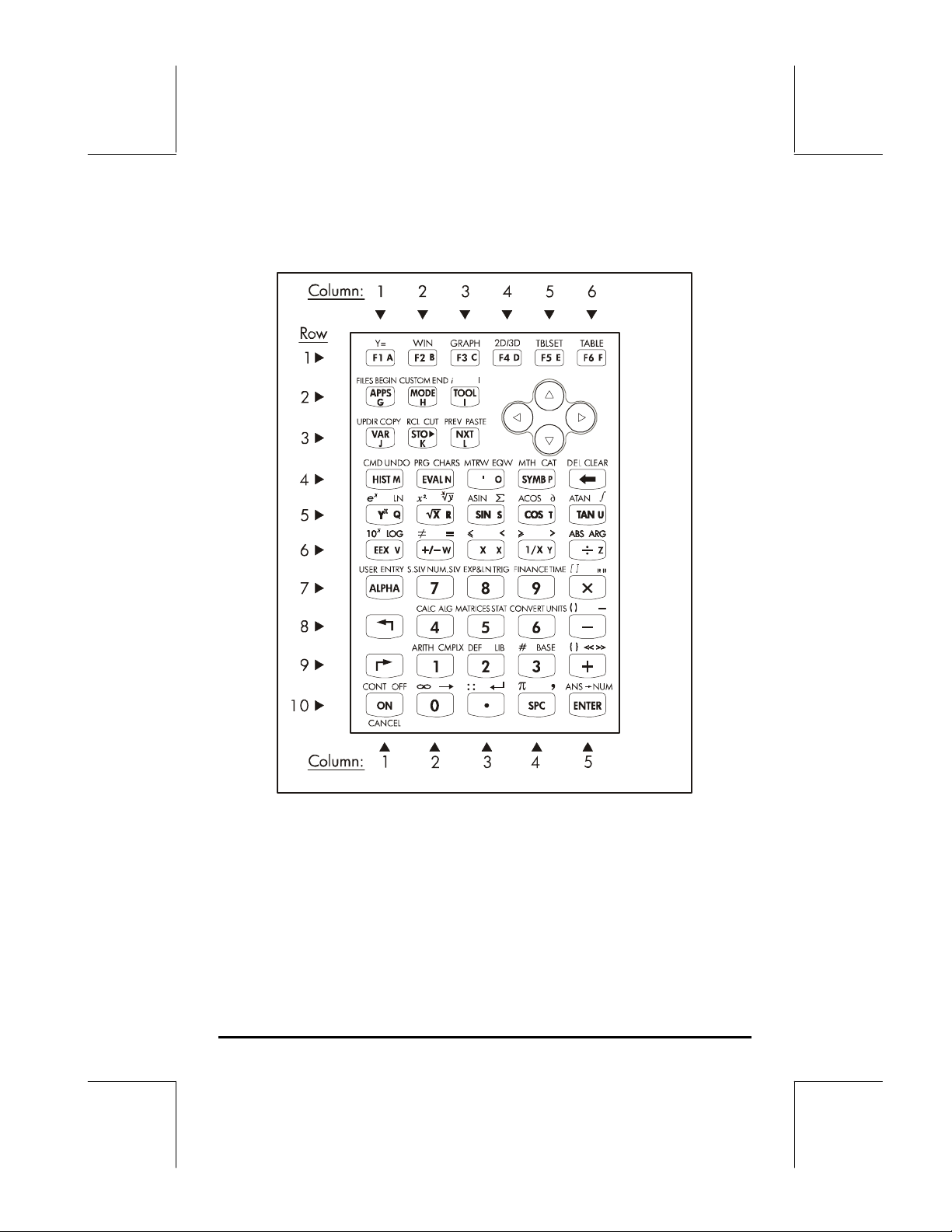
the blue ALPHA key, key (7,1), can be combined with some of the other keys to activate the alternative functions shown in the keyboard.

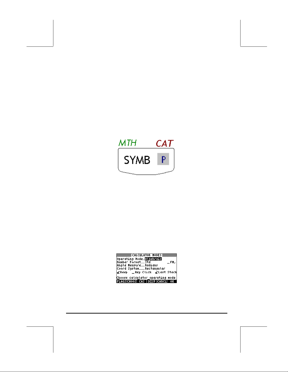
For example, the P key, key(4,4), has the following six functions associated with it:

P Main function, to activate the SYMBolic menu „´ Left-shift function, to activate the MTH (Math) menu … N Right-shift function, to activate the CATalog function

Page 1-5

~p ALPHA function, to enter the upper-case letter P ~„p ALPHA-Left-Shift function, to enter the lower-case letter p ~…p ALPHA-Right-Shift function, to enter the symbol π

Of the six functions associated with a key only the first four are shown in the keyboard itself. The figure in next page shows these four labels for the P key. Notice that the color and the position of the labels in the key, namely, SYMB, MTH, CAT and P, indicate which is the main function (SYMB), and which of the other three functions is associated with the left-shift „(MTH), right-shift … (CAT ), and ~ (P) keys.

For detailed information on the calculator keyboard operation refer to Appendix B in the calculator’s user’s guide.

Selecting calculator modes

This section assumes that you are now at least partially familiar with the use of choose and dialog boxes (if you are not, please refer to appendix A in the user’s guide).

Press the H button (second key from the left on the second row of keys from the top) to show the following CALCULATOR MODES input form:

Page 1-6

Press the !!@@OK#@ ( F) soft menu key to return to normal display. Examples of selecting different calculator modes are shown next.

Operating Mode

The calculator offers two operating modes: the Algebraic mode, and the Reverse Polish Notation (RPN) mode. The default mode is the Algebraic

mode (as indicated in the figure above), however, users of earlier HP calculators may be more familiar with the RPN mode.

To select an operating mode, first open the CALCULATOR MODES input form by pressing the H button. The Operating Mode field will be highlighted. Select the Algebraic or RPN operating mode by either using the \ key (second from left in the fifth row from the keyboard bottom), or pressing the @CHOOS soft menu key ( B). If using the latter approach, use up and down arrow keys, — ˜, to select the mode, and press the !!@@OK#@ soft menu key to complete the operation.

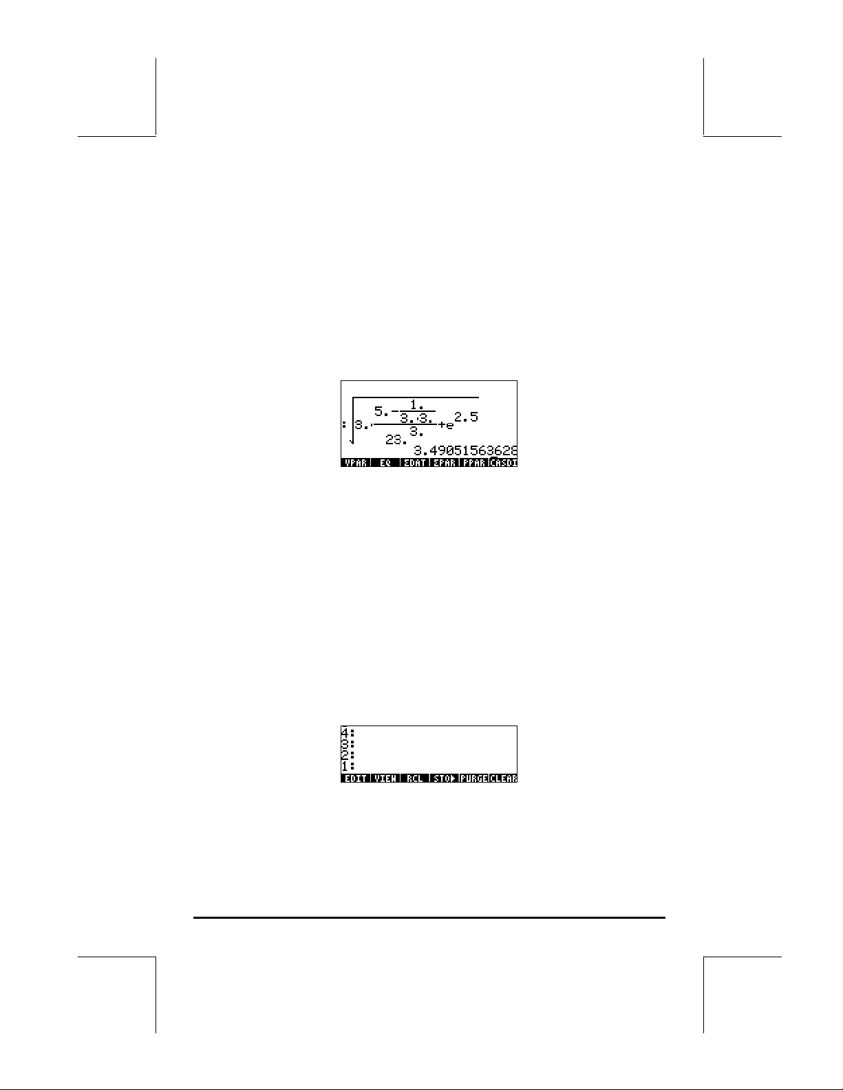
To illustrate the difference between these two operating modes we will calculate the following expression in both modes:



0.50.3

−⋅

 

0.23

To enter this expression in the calculator we will first use the equation writer, ‚O. Please identify the following keys in the keyboard, besides the numeric keypad keys:

!@.#*+-/R

Q¸Ü‚Oš™˜—`

The equation writer is a display mode in which you can build mathematical expressions using explicit mathematical notation including fractions, derivatives, integrals, roots, etc. To use the equation writer for writing the expression shown above, use the following keystrokes:

‚OR3.*!Ü5.-

 

0.30.3

⋅



5.2

Page 1-7

1./3.*3. —————

/23.Q3™™+!¸2.5`

After pressing `the calculator displays the expression:

√ (3.*(5.-1/(3.*3.))/23.^3+EXP(2.5))

Pressing `again will provide the following value (accept Approx mode on, if asked, by pressing !!@@OK#@):

You could also type the expression directly into the display without using the equation writer, as follows:

R!Ü3.*!Ü5.-

1/3.*3.™

/23.Q3+!¸2.5`

to obtain the same result.

Change the operating mode to RPN by first pressing the H button. Select the RPN operating mode by either using the \key, or pressing the @CHOOS soft menu key. Press the @@OK#@ ( F) soft menu key to complete the operation. The display, for the RPN mode looks as follows:

Notice that the display shows several levels of output labeled, from bottom to top, as 1, 2, 3, etc. This is referred to as the stack of the calculator. The

Page 1-8

different levels are referred to as the stack levels, i.e., stack level 1, stack level 2, etc.

Basically, what RPN means is that, instead of writing an operation such as 3 + 2, in the calculator by using

3+2`

we write first the operands, in the proper order, and then the operator, i.e.,

3`2`+

As you enter the operands, they occupy different stack levels. Entering 3`puts the number 3 in stack level 1. Next, entering 2`pushes the 3 upwards to occupy stack level 2. Finally, by pressing +, we are telling the calculator to apply the operator, or program, + to the objects occupying levels 1 and 2. The result, 5, is then placed in level 1.

Let's try some other simple operations before trying the more complicated expression used earlier for the algebraic operating mode:

123/32 123`32/

4`2Q

√(√27) 27`R3@»

Notice the position of the y and the x in the last two operations. The base in the exponential operation is y (stack level 2) while the exponent is x (stack level 1) before the key Q is pressed. Similarly, in the cubic root operation, y (stack level 2) is the quantity under the root sign, and x (stack level 1) is the root.

Try the following exercise involving 3 factors: (5 + 3) × 2

5`3`+ Calculates (5 +3) first. 2X Completes the calculation.

Let's try now the expression proposed earlier:

Page 1-9



 



−⋅



⋅



5.2

3` Enter 3 in level 1 5` Enter 5 in level 1, 3 moves to level 2 3` Enter 3 in level 1, 5 moves to level 2, 3 to level 3 3* Place 3 and multiply, 9 appears in level 1 Y 1/(3×3), last value in lev. 1; 5 in level 2; 3 in level 3

- 5 - 1/(3×3) , occupies level 1 now; 3 in level 2 * 3× (5 - 1/(3×3)), occupies level 1 now. 23` Enter 23 in level 1, 14.66666 moves to level 2. 3Q Enter 3, calculate 23 / (3× (5-1/(3×3)))/23

into level 1. 14.666 in lev. 2.

into level 1

2.5 Enter 2.5 level 1 !¸ e + (3× (5 - 1/(3×3)))/23 R √((3× (5 - 1/(3×3)))/23

2.5

, goes into level 1, level 2 shows previous value.

2.5

= 12.18369, into lev. 1.

2.5

) = 3.4905156, into 1.

To select between the ALG vs. RPN operating mode, you can also set/clear system flag 95 through the following keystroke sequence:

H @)FLAGS —„—„—„— @@CHK@@

Number Format and decimal dot or comma

Changing the number format allows you to customize the way real numbers are displayed by the calculator. You will find this feature extremely useful in operations with powers of tens or to limit the number of decimals in a result.

To select a number format, first open the CALCULATOR MODES input form by pressing the H button. Then, use the down arrow key, ˜, to select the option Number format. The default value is Std, or Standard format. In the standard format, the calculator will show floating-point numbers with no set decimal placement and with the maximum precision allowed by the calculator

Page 1-10

(12 significant digits).”To learn more about reals, see Chapter 2 in this guide. To illustrate this and other number formats try the following exercises:

• Standard format:

This mode is the most used mode as it shows numbers in the most familiar notation. Press the !!@@OK#@ soft menu key, with the Number format set to Std, to return to the calculator display. Enter the number

123.4567890123456 (with16 significant figures). Press the ` key. The number is rounded to the maximum 12 significant figures, and is displayed as follows:

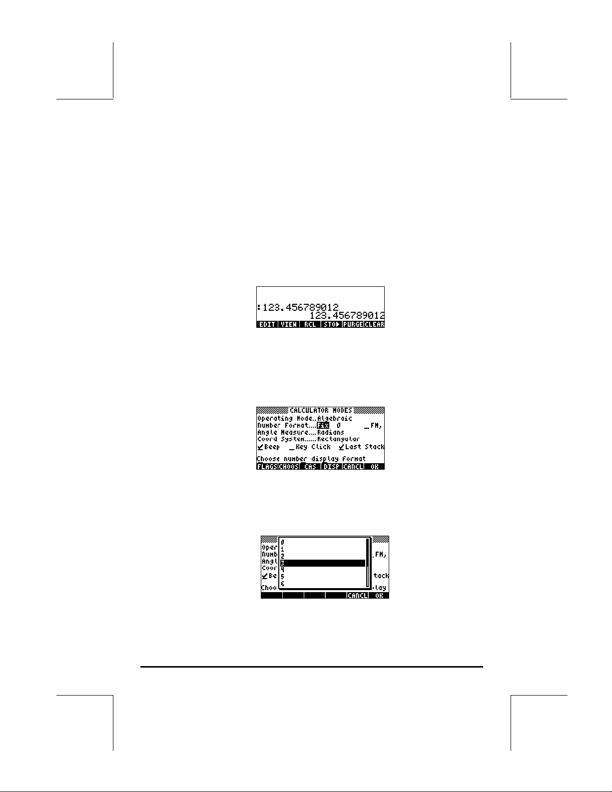
• Fixed format with decimals:

Press the H button. Next, use the down arrow key, ˜, to select the option Number format. Press the @CHOOS soft menu key ( B), and select the option Fixed with the arrow down key ˜.

Press the right arrow key, ™, to highlight the zero in front of the option Fix. Press the @CHOOS soft menu key and, using the up and down arrow keys, —˜, select, say, 3 decimals.

Page 1-11

Press the !!@@OK#@ soft menu key to complete the selection:

Press the !!@@OK#@ soft menu key return to the calculator display. The number now is shown as:

Notice how the number is rounded, not truncated. Thus, the number

123.4567890123456, for this setting, is displayed as 123.457, and not as 123.456 because the digit after 6 is > 5.

• Scientific format

To set this format, start by pressing the H button. Next, use the down arrow key, ˜, to select the option Number format. Press the @CHOOS soft menu key ( B), and select the option Scientific with the arrow down key ˜. Keep the number 3 in front of the Sci. (This number can be changed in the same fashion that we changed the Fixed number of decimals in the example above).

Press the !!@@OK#@ soft menu key return to the calculator display. The number now is shown as:

Page 1-12

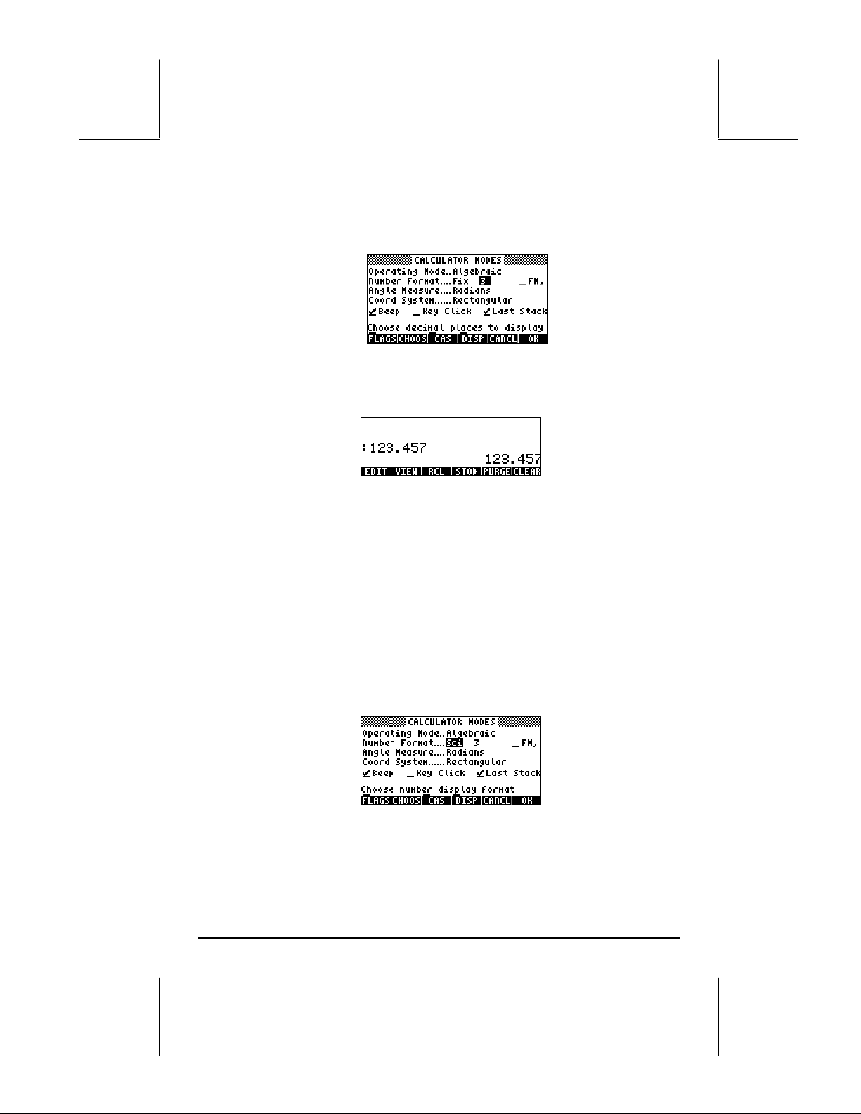
This result, 1.23E2, is the calculator’s version of powers-of-ten notation, i.e., 1.235 × 10

. In this, so-called, scientific notation, the number 3 in front of the Sci number format (shown earlier) represents the number of significant figures after the decimal point. Scientific notation always includes one integer figure as shown above. For this case, therefore, the number of significant figures is four.

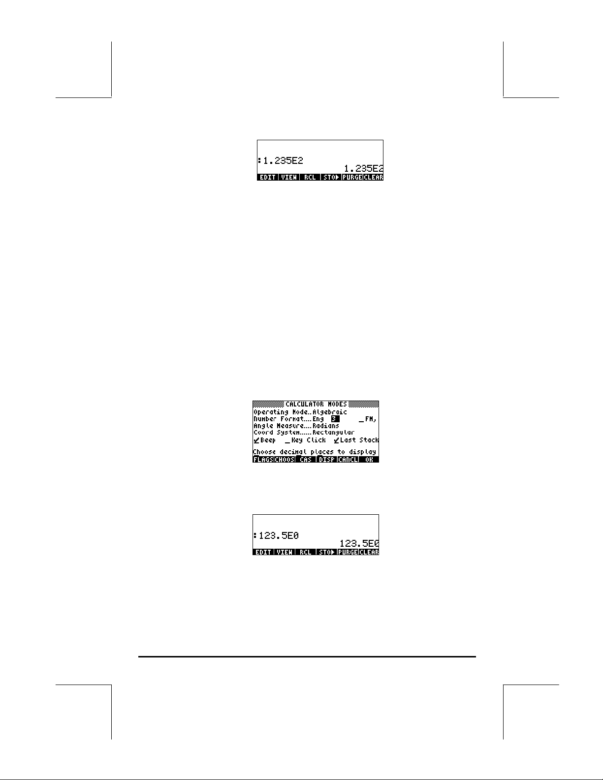
• Engineering format

The engineering format is very similar to the scientific format, except that the powers of ten are multiples of three. To set this format, start by pressing the H button. Next, use the down arrow key, ˜, to select the option Number format. Press the @CHOOS soft menu key ( B), and select the option Engineering with the arrow down key ˜. Keep the number 3 in front of the Eng. (This number can be changed in the same fashion that we changed the Fixed number of decimals in an earlier example).

Press the !!@@OK#@ soft menu key return to the calculator display. The number now is shown as:

Because this number has three figures in the integer part, it is shown with four significative figures and a zero power of ten, while using the Engineering format. For example, the number 0.00256, will be shown as:

Page 1-13

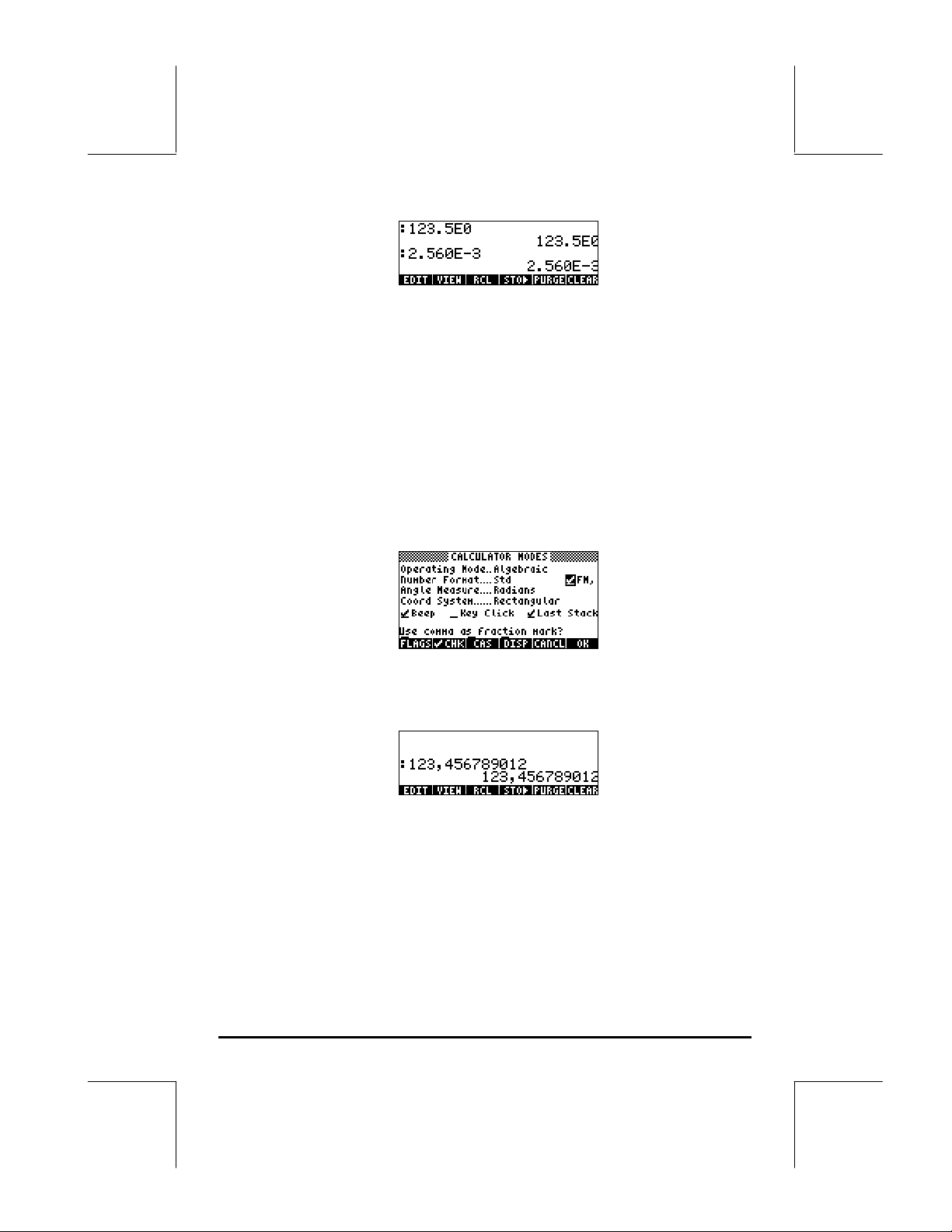
• Decimal comma vs. decimal point

Decimal points in floating-point numbers can be replaced by commas, if the user is more familiar with such notation. To replace decimal points for commas, change the FM option in the CALCULATOR MODES input form to commas, as follows (Notice that we have changed the Number Format to Std):

• Press the H button. Next, use the down arrow key, ˜, once, and the

right arrow key, ™, highlighting the option __FM,. To select commas, press the @@CHK@@ soft menu key (i.e., the B key). The input form will look as follows:

• Press the !!@@OK#@ soft menu key return to the calculator display. The

number 123.4567890123456, entered earlier, now is shown as:

Angle Measure

Trigonometric functions, for example, require arguments representing plane angles. The calculator provides three different Angle Measure modes for working with angles, namely:

• Degrees: There are 360 degrees (360

• Radians: There are 2π radians (2π

) in a complete circumference.

Page 1-14

• Grades: There are 400 grades (400 g) in a complete circumference.

The angle measure affects the trig functions like SIN, COS, TAN and associated functions.

To change the angle measure mode, use the following procedure:

• Press the H button. Next, use the down arrow key, ˜, twice. Select

the Angle Measure mode by either using the \key (second from left in the fifth row from the keyboard bottom), or pressing the @CHOOS soft menu key ( B). If using the latter approach, use up and down arrow keys,— ˜, to select the preferred mode, and press the !!@@OK#@ (F) soft menu key to complete the operation. For example, in the following screen, the Radians mode is selected:

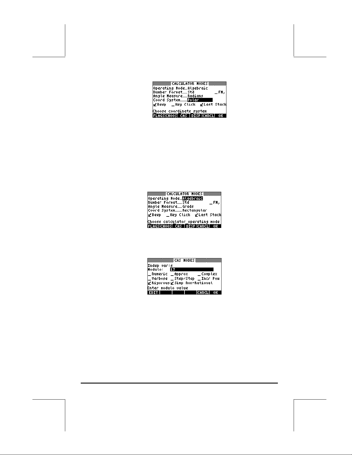
Coordinate System

The coordinate system selection affects the way vectors and complex numbers are displayed and entered. To learn more about complex numbers and vectors, see Chapters 4 and 8, respectively, in this guide. There are three coordinate systems available in the calculator: Rectangular (RECT), Cylindrical (CYLIN), and Spherical (SPHERE). To change coordinate system:

• Press the H button. Next, use the down arrow key, ˜, three times.

Select the Coord System mode by either using the \ key (second from left in the fifth row from the keyboard bottom), or pressing the @CHOOS soft menu key ( B). If using the latter approach, use up and down arrow keys,— ˜, to select the preferred mode, and press the !!@@OK#@ ( F) soft menu key to complete the operation. For example, in the following screen, the Polar coordinate mode is selected:

Page 1-15

Selecting CAS settings

CAS stands for Computer Algebraic System. This is the mathematical core of the calculator where the symbolic mathematical operations and functions are programmed. The CAS offers a number of settings can be adjusted according to the type of operation of interest. To see the optional CAS settings use the following:

• Press the H button to activate the CALCULATOR MODES input form.

• To change CAS settings press the @@ CAS@@ soft menu key. The default values

of the CAS setting are shown below:

• To navigate through the many options in the CAS MODES input form, use

the arrow keys: š™˜—.

• To select or deselect any of the settings shown above, select the underline

before the option of interest, and toggle the @@CHK@@ soft menu key until the right setting is achieved. When an option is selected, a check mark will be shown in the underline (e.g., the Rigorous and Simp Non-Rational

Page 1-16

options above). Unselected options will show no check mark in the underline preceding the option of interest (e.g., the _Numeric, _Approx, _Complex, _Verbose, _Step/Step, _Incr Pow options above).

• After having selected and unselected all the options that you want in the

CAS MODES input form, press the @@@OK@@@ soft menu key. This will take you back to the CALCULATOR MODES input form. To return to normal calculator display at this point, press the @@@OK@@@ soft menu key once more.

Explanation of CAS settings

• Indep var: The independent variable for CAS applications. Typically, VX

= ‘X’.

• Modulo

modulus or modulo of the arithmetic ring (see Chapter 5 in the calculator’s user’s guide).

• Numeric

in calculations.

• Approx

unchecked, the CAS is in Exact mode, which produces symbolic results in algebraic calculations.

• Complex

CAS is in Real mode, i.e., real number calculations are the default. See Chapter 4 for operations with complex numbers.

• Verbose

• Step/Step

Useful to see intermediate steps in summations, derivatives, integrals, polynomial operations (e.g., synthetic division), and matrix operations.

• Incr Pow

shown in increasing order of the powers of the independent variable.

• Rigorous

|X| to X.

• Simp Non-Rational

expressions as much as possible.

: For operations in modular arithmetic this variable holds the

: If set, the calculator produces a numeric, or floating-point result,

: If set, Approximate mode uses numerical results in calculations. If

: If set, complex number operations are active. If unchecked the

: If set, provides detailed information in certain CAS operations.

: If set, provides step-by-step results for certain CAS operations.

: Increasing Power, means that, if set, polynomial terms are

: If set, calculator does not simplify the absolute value function

: If set, the calculator will try to simplify non-rational

Selecting Display modes

Page 1-17

The calculator display can be customized to your preference by selecting different display modes. To see the optional display settings use the following:

• First, press the H button to activate the CALCULATOR MODES input

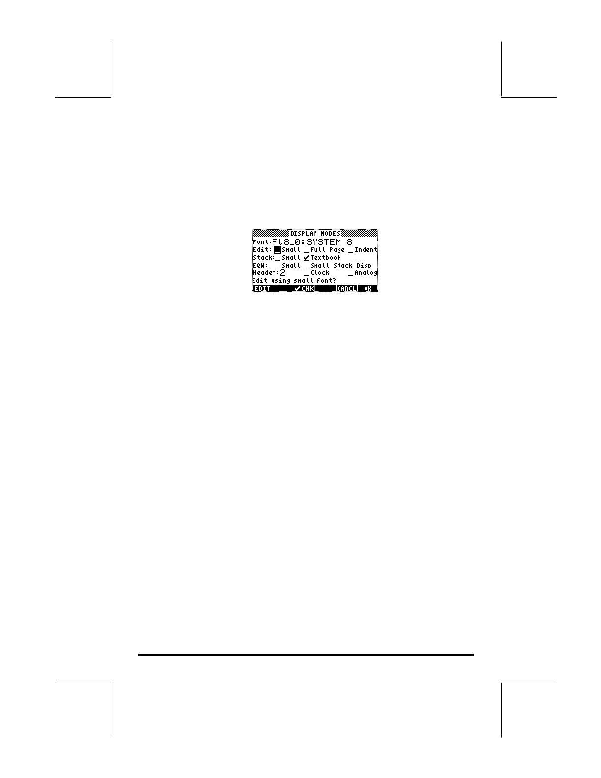
form. Within the CALCULATOR MODES input form, press the @@DISP@ soft menu key (D) to display the DISPLAY MODES input form.

• To navigate through the many options in the DISPLAY MODES input form,

use the arrow keys: š™˜—.

• To select or deselect any of the settings shown above, that require a check

mark, select the underline before the option of interest, and toggle the @CHK@@ soft menu key until the right setting is achieved. When an option is selected, a check mark will be shown in the underline (e.g., the Textbook option in the Stack: line above). Unselected options will show no check mark in the underline preceding the option of interest (e.g., the _Small, _Full page, and _Indent options in the Edit: line above).

• To select the Font for the display, highlight the field in front of the Font:

option in the DISPLAY MODES input form, and use the @CHOOS soft menu key (B).

• After having selected and unselected all the options that you want in the

DISPLAY MODES input form, press the @@@OK@@@ soft menu key. This will take you back to the CALCULATOR MODES input form. To return to normal calculator display at this point, press the @@@OK@@@ soft menu key once more.

Selecting the display font

First, press the H button to activate the CALCULATOR MODES input form. Within the CALCULATOR MODES input form, press the @@DISP@ soft menu key

Page 1-18

(D) to display the DISPLAY MODES input form. The Font: field is highlighted, and the option Ft8_0:system 8 is selected. This is the default value of the display font. Pressing the @CHOOS soft menu key (B), will provide a list of available system fonts, as shown below:

The options available are three standard System Fonts (sizes 8, 7, and 6) and a Browse.. option. The latter will let you browse the calculator memory for additional fonts that you may have created or downloaded into the calculator.

Practice changing the display fonts to sizes 7 and 6. Press the OK soft menu key to effect the selection. When done with a font selection, press the @@@OK@@@ soft menu key to go back to the CALCULATOR MODES input form. To return to normal calculator display at this point, press the @@@OK@@@ soft menu key once more and see how the stack display change to accommodate the different font.

Selecting properties of the line editor

First, press the H button to activate the CALCULATOR MODES input form. Within the CALCULATOR MODES input form, press the @@DISP@ soft menu key (D) to display the DISPLAY MODES input form. Press the down arrow key, ˜, once, to get to the Edit line. This line shows three properties that can be modified. When these properties are selected (checked) the following effects are activated:

_Small Changes font size to small _Full page Allows to place the cursor after the end of the line _Indent Auto indent cursor when entering a carriage return

Instructions on the use of the line editor are presented in Chapter 2 in the user’s guide.

Page 1-19

Selecting properties of the Stack

First, press the H button to activate the CALCULATOR MODES input form. Within the CALCULATOR MODES input form, press the @@DISP@ soft menu key (D) to display the DISPLAY MODES input form. Press the down arrow key, ˜, twice, to get to the Stack line. This line shows two properties that can be modified. When these properties are selected (checked) the following effects are activated:

_Small Changes font size to small. This maximizes the amount of

information displayed on the screen. Note, this selection overrides the font selection for the stack display.

_Textbook Displays mathematical expressions in graphical mathematical

notation

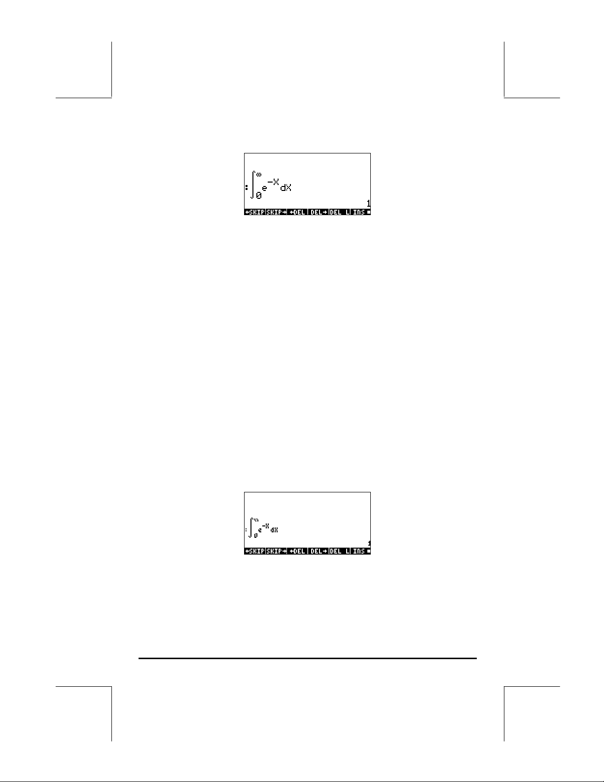
To illustrate these settings, either in algebraic or RPN mode, use the equation writer to type the following definite integral:

‚O…Á0™„è™„¸\x™x`

In Algebraic mode, the following screen shows the result of these keystrokes with neither _Small nor _Textbook are selected:

With the _Small option selected only, the display looks as shown below:

With the _Textbook option selected (default value), regardless of whether the _Small option is selected or not, the display shows the following result:

Page 1-20

Selecting properties of the equation writer (EQW)

First, press the H button to activate the CALCULATOR MODES input form. Within the CALCULATOR MODES input form, press the @@DISP@ soft menu key (D) to display the DISPLAY MODES input form. Press the down arrow key, ˜, three times, to get to the EQW (Equation Writer) line. This line shows two properties that can be modified. When these properties are selected (checked) the following effects are activated:

_Small Changes font size to small while using the equation

editor

_Small Stack Disp Shows small font in the stack after using the equation

editor

Detailed instructions on the use of the equation editor (EQW) are presented elsewhere in this manual.

∞

−

For the example of the integral

_Small Stack Disp in the EQW line of the DISPLAY MODES input form produces the following display:

dXe

∫

, presented above, selecting the

References

Additional references on the subjects covered in this Chapter can be found in Chapter 1 and Appendix C of the calculator’s user’s guide.

Page 1-21

Chapter 2 Introducing the calculator

In this chapter we present a number of basic operations of the calculator including the use of the Equation Writer and the manipulation of data objects in the calculator. Study the examples in this chapter to get a good grasp of the capabilities of the calculator for future applications.

Calculator objects

Some of the most commonly used objects are: reals (real numbers, written with a decimal point, e.g., -0.0023, 3.56), integers (integer numbers, written without a decimal point, e.g., 1232, -123212123), complex numbers (written as an ordered pair, e.g., (3,-2)), lists, etc. Calculator objects are described in Chapters 2 and 24 in the calculator’s user guide.

Editing expressions in the stack

In this section we present examples of expression editing directly into the calculator display or stack.

Creating arithmetic expressions

For this example, we select the Algebraic operating mode and select a Fix format with 3 decimals for the display. We are going to enter the arithmetic expression:

0.1

0.5

⋅

To enter this expression use the following keystrokes:

5.*„Ü1.+1/7.5™/ „ÜR3.-2.Q3

The resulting expression is: 5*(1+1/7.5)/( ƒ3-2^3).

Press ` to get the expression in the display as follows:

5.7

0.20.3

−

Page 2-1

Notice that, if your CAS is set to EXACT (see Appendix C in user’s guide) and you enter your expression using integer numbers for integer values, the result is a symbolic quantity, e.g.,

5*„Ü1+1/7.5™/

„ÜR3-2Q3

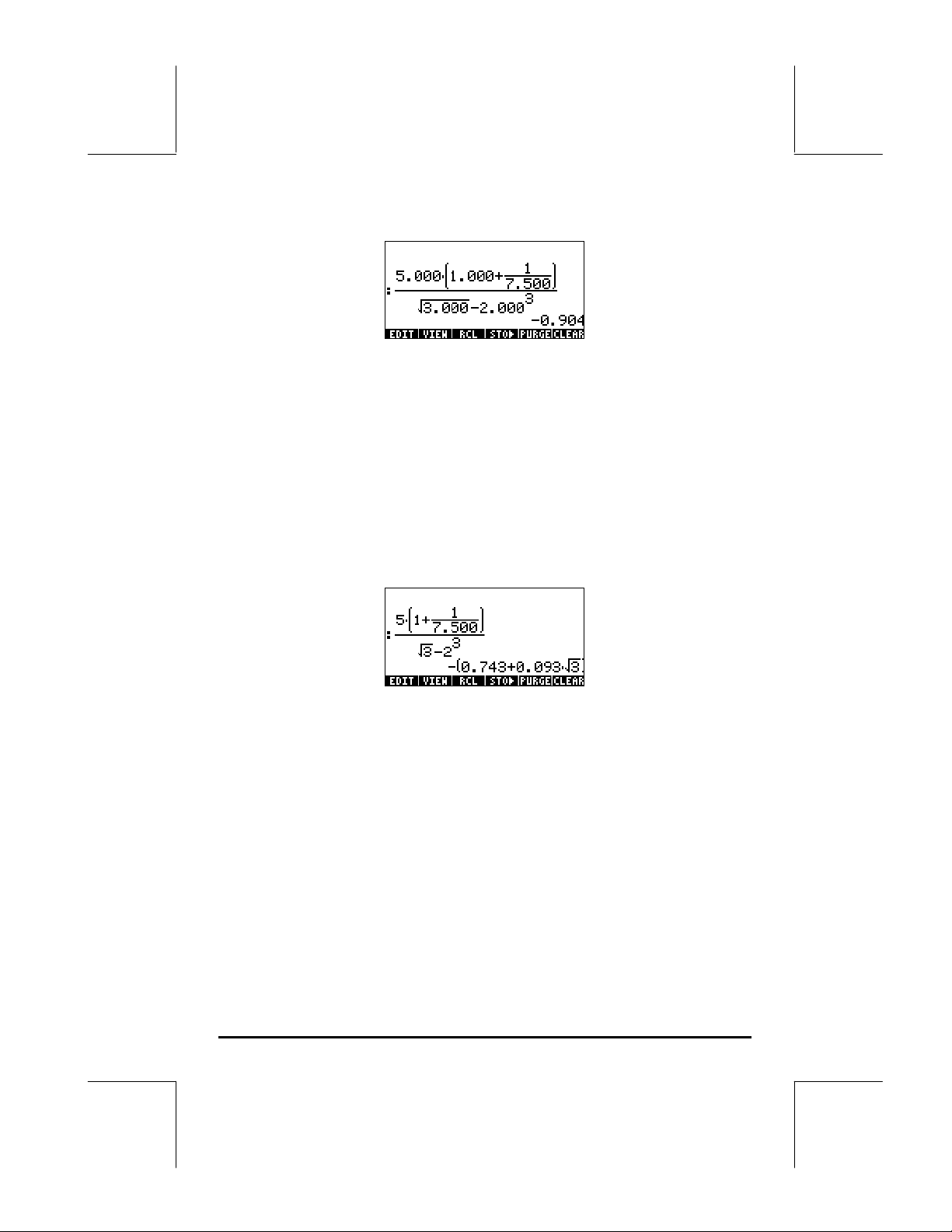
Before producing a result, you will be asked to change to Approximate mode. Accept the change to get the following result (shown in Fix decimal mode with three decimal places – see Chapter 1):

In this case, when the expression is entered directly into the stack, as soon as you press `, the calculator will attempt to calculate a value for the expression. If the expression is entered between apostrophes, however, the calculator will reproduce the expression as entered. For example:

³5*„Ü1+1/7.5™/

„ÜR3-2Q3`

The result will be shown as follows:

Page 2-2

To evaluate the expression we can use the EVAL function, as follows:

µ„î`

If the CAS is set to Exact, you will be asked to approve changing the CAS setting to Approx. Once this is done, you will get the same result as before.

An alternative way to evaluate the expression entered earlier between quotes is by using the option …ï.

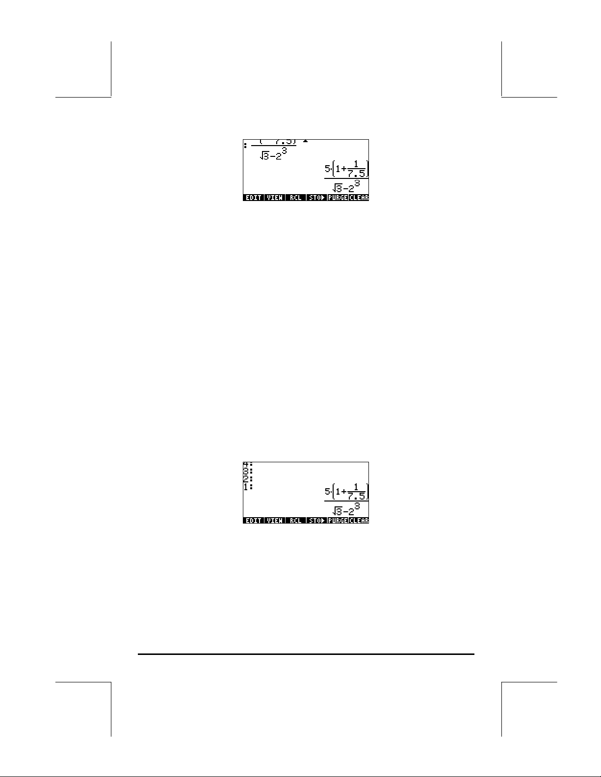
We will now enter the expression used above when the calculator is set to the RPN operating mode. We also set the CAS to Exact, the display to Textbook, and the number format to Standard. The keystrokes to enter the expression between quotes are the same used earlier, i.e.,

³5*„Ü1+1/7.5™/

„ÜR3-2Q3`

Resulting in the output

Press ` once more to keep two copies of the expression available in the stack for evaluation. We first evaluate the expression using the function EVAL, and next using the function NUM: µ.

Page 2-3

This expression is semi-symbolic in the sense that there are floating-point components to the result, as well as a √3. Next, we switch stack locations [using ™] and evaluate using function NUM, i.e., ™…ï.

This latter result is purely numerical, so that the two results in the stack, although representing the same expression, seem different. To verify that they are not, we subtract the two values and evaluate this difference using function EVAL: -µ. The result is zero (0.).

For additional information on editing arithmetic expressions in the display or stack, see Chapter 2 in the calculator’s user’s guide.

Creating algebraic expressions

Algebraic expressions include not only numbers, but also variable names. As an example, we will enter the following algebraic expression:

L212

We set the calculator operating mode to Algebraic, the CAS to Exact, and the display to Textbook. To enter this algebraic expression we use the following keystrokes:

³2*~l*R„Ü1+~„x/~r™/ „ Ü ~r+~„y™+2*~l/~„b

Press ` to get the following result:

Page 2-4

Entering this expression when the calculator is set in the RPN mode is exactly the same as this Algebraic mode exercise.

For additional information on editing algebraic expressions in the calculator’s display or stack see Chapter 2 in the calculator’s user’s guide.

Using the Equation Writer (EQW) to create expressions

The equation writer is an extremely powerful tool that not only let you enter or see an equation, but also allows you to modify and work/apply functions on all or part of the equation.

The Equation Writer is launched by pressing the keystroke combination ‚O (the third key in the fourth row from the top in the keyboard). The resulting screen is the following. Press L to see the second menu page:

The six soft menu keys for the Equation Writer activate functions EDIT, CURS, BIG, EVAL, FACTOR, SIMPLIFY, CMDS, and HELP. Detailed information on these functions is provided in Chapter 3 of the calculator’s user’s guide.

Creating arithmetic expressions

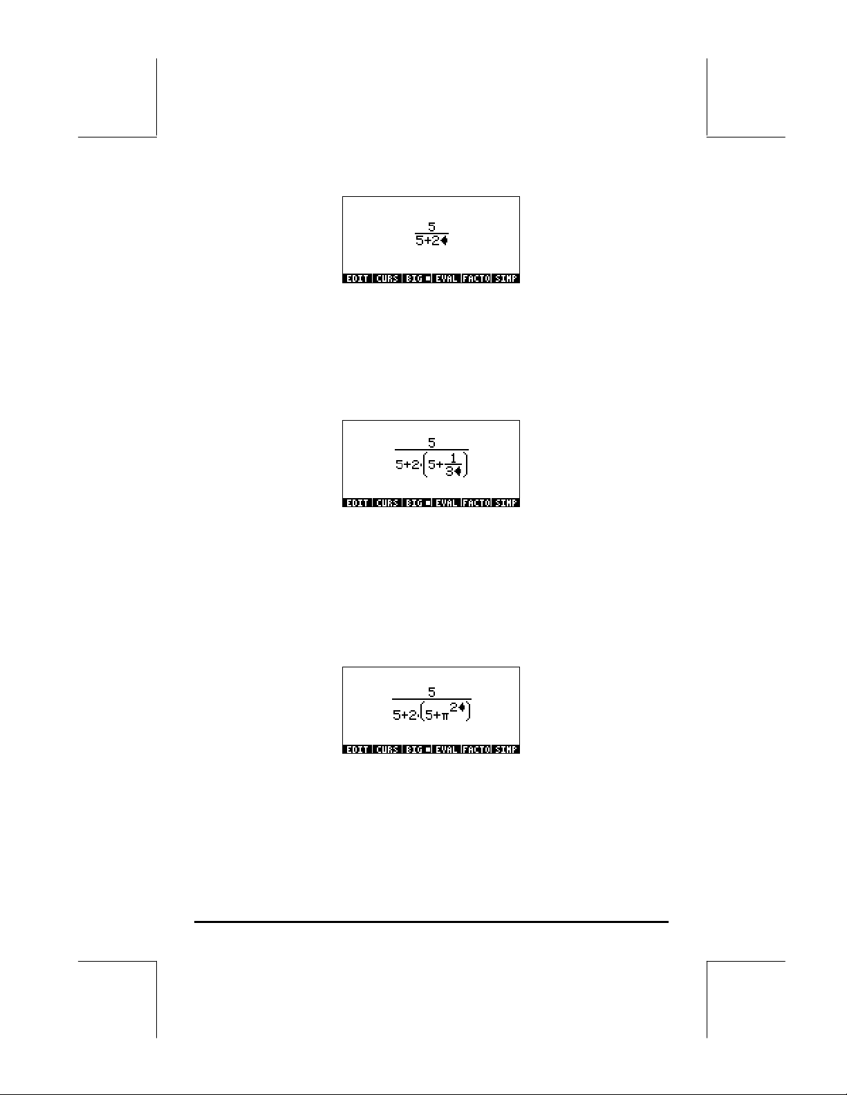
Entering arithmetic expressions in the Equation Writer is very similar to entering an arithmetic expression in the stack enclosed in quotes. The main difference is that in the Equation Writer the expressions produced are written in “textbook” style instead of a line-entry style. For example, try the following keystrokes in the Equation Writer screen: 5/5+2

The result is the expression

Page 2-5

The cursor is shown as a left-facing key. The cursor indicates the current edition location. For example, for the cursor in the location indicated above, type now:

*„Ü5+1/3

The edited expression looks as follows:

Suppose that you want to replace the quantity between parentheses in the denominator (i.e., 5+1/3) with (5+π

/2). First, we use the delete key (ƒ)

delete the current 1/3 expression, and then we replace that fraction with π as follows:

ƒƒƒ„ìQ2

When hit this point the screen looks as follows:

In order to insert the denominator 2 in the expression, we need to highlight the entire π

expression. We do this by pressing the right arrow key (™)

once. At that point, we enter the following keystrokes:

/2,

Page 2-6

The expression now looks as follows:

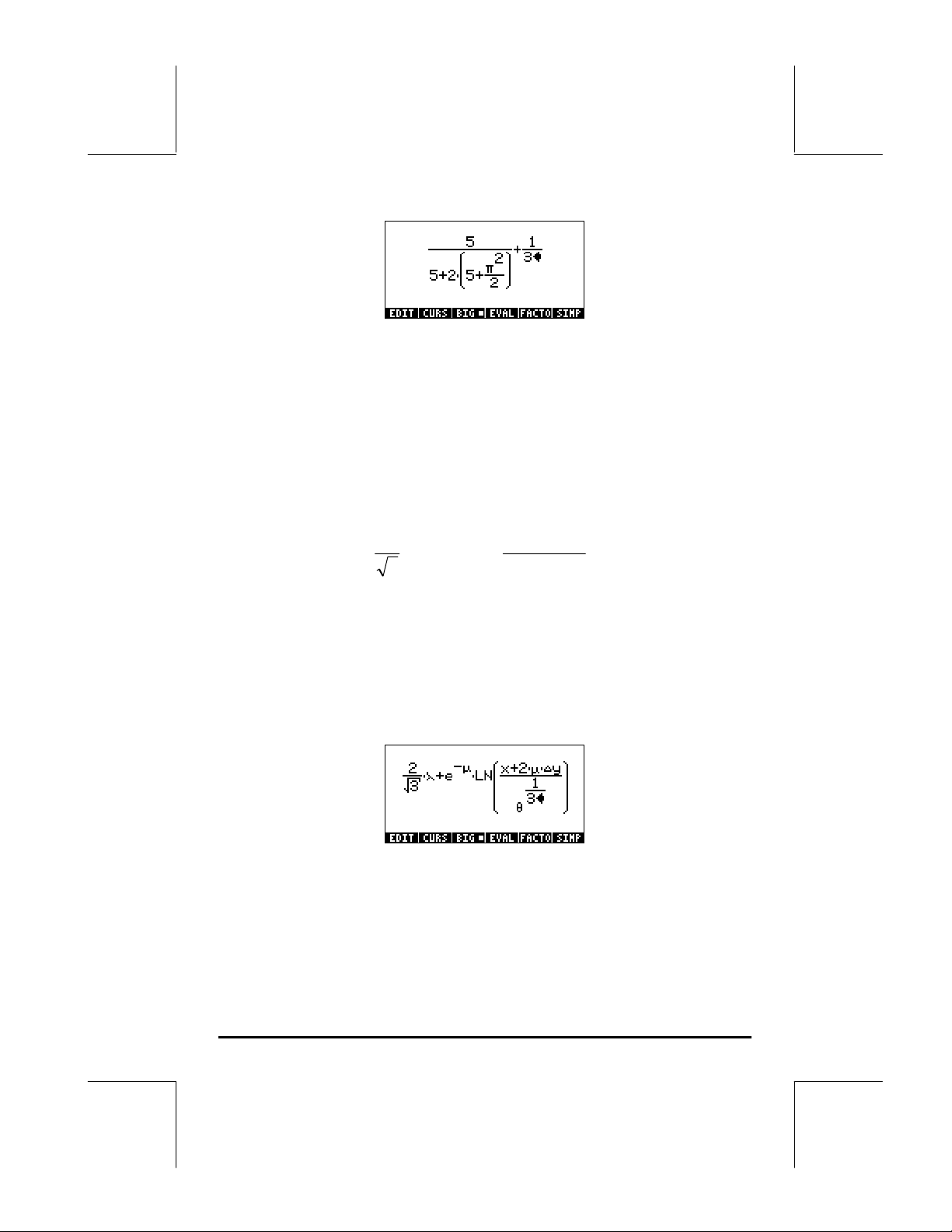
Suppose that now you want to add the fraction 1/3 to this entire expression, i.e., you want to enter the expression:

5(25

+⋅+

)

First, we need to highlight the entire first term by using either the right arrow (™) or the upper arrow (—) keys, repeatedly, until the entire expression is highlighted, i.e., seven times, producing:

NOTE: Alternatively, from the original position of the cursor (to the right of the 2 in the denominator of π2/2), we can use the keystroke combination ‚— , interpreted as (‚ ‘ ).

Once the expression is highlighted as shown above, type +1/3 to add the fraction 1/3. Resulting in:

Page 2-7

Creating algebraic expressions

An algebraic expression is very similar to an arithmetic expression, except that English and Greek letters may be included. The process of creating an algebraic expression, therefore, follows the same idea as that of creating an arithmetic expression, except that use of the alphabetic keyboard is included.

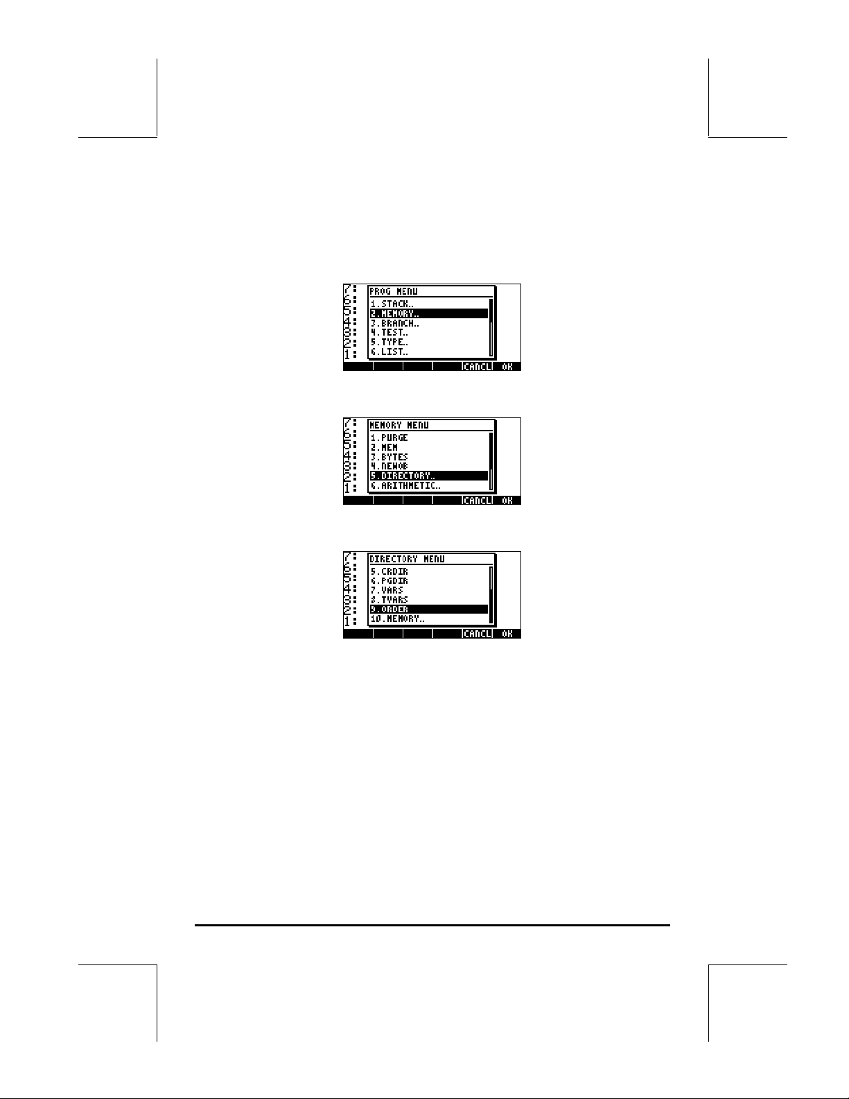
To illustrate the use of the Equation Writer to enter an algebraic equation we will use the following example. Suppose that we want to enter the expression:

∆⋅+

−

⋅+

LNe

Use the following keystrokes:

2 / R3 ™™ * ~‚n + „¸\ ~‚m

™™ * ‚¹ ~„x + 2 * ~‚m * ~‚c

~„y ——— / ~‚t Q1/3

This results in the output:

 



 

3/1



In this example we used several lower-case English letters, e.g., x (~„x), several Greek letters, e.g., λ (~‚n), and even a combination of Greek and English letters, namely, ∆y (~‚c ~„y). Keep in mind that to enter a lower-case English letter, you need to use the combination: ~„ followed by the letter you want to enter.

Page 2-8

Also, you can always copy special characters by using the CHARS menu (…±) if you don’t want to memorize the keystroke combination that produces it. A listing of commonly used ~‚keystroke combinations is listed in Appendix D of the user’s guide.

For additional information on editing, evaluating, factoring, and simplifying algebraic expressions see Chapter 2 of the calculator’s user’s guide.

Organizing data in the calculator

You can organize data in your calculator by storing variables in a directory tree. The basis of the calculator’s directory tree is the HOME directory described next.

The HOME directory

To get to the HOME directory, press the UPDIR function („§) -- repeat as needed -- until the {HOME} spec is shown in the second line of the display header. Alternatively, use „ (hold) §. For this example, the HOME directory contains nothing but the CASDIR. Pressing J will show the variables in the soft menu keys:

Subdirectories

To store your data in a well organized directory tree you may want to create subdirectories under the HOME directory, and more subdirectories within subdirectories, in a hierarchy of directories similar to folders in modern computers. The subdirectories will be given names that may reflect the contents of each subdirectory, or any arbitrary name that you can think off. For details on manipulation of directories see Chapter 2 in the calculator’s user’s guide.

Page 2-9

Variables

Variables are similar to files on a computer hard drive. One variable can store one object (numerical values, algebraic expressions, lists, vectors, matrices, programs, etc). Variables are referred to by their names, which can be any combination of alphabetic and numerical characters, starting with a letter (either English or Greek). Some non-alphabetic characters, such as the arrow (→) can be used in a variable name, if combined with an alphabetical character. Thus, ‘→A’ is a valid variable name, but ‘→’ is not. Valid examples of variable names are: ‘A’, ‘B’, ‘a’, ‘b’, ‘α’, ‘β’, ‘A1’, ‘AB12’, ‘A12’,’Vel’,’Z0’,’z1’, etc.

A variable can not have the same name as a function of the calculator. Some of the reserved calculator variable names are the following: ALRMDAT, CST, EQ, EXPR, IERR, IOPAR, MAXR, MINR, PICT, PPAR, PRTPAR, VPAR, ZPAR, der_, e, i, n1,n2, …, s1, s2, …, ΣDAT, ΣPAR, π, ∞

Variables can be organized into sub-directories (see Chapter 2 in the calculator’s user’s guide).

Typing variable names

To name variables, you will have to type strings of letters at once, which may or may not be combined with numbers. To type strings of characters you can lock the alphabetic keyboard as follows:

~~ locks the alphabetic keyboard in upper case. When locked in this fashion, pressing the „ before a letter key produces a lower case letter, while pressing the ‚ key before a letter key produces a special character. If the alphabetic keyboard is already locked in upper case, to lock it in lower case, type, „~

~~„~ locks the alphabetic keyboard in lower case. When locked in this fashion, pressing the „ before a letter key produces an upper case letter. To unlock lower case, press „~

Page 2-10

To unlock the upper-case locked keyboard, press ~

Try the following exercises:

³~~math` ³~~m„a„t„h` ³~~m„~at„h`

The calculator display will show the following (left-hand side is Algebraic mode, right-hand side is RPN mode):

Creating variables

The simplest way to create a variable is by using the K . The following examples are used to store the variables listed in the following table (Press J if needed to see variables menu):

Name Contents Type

A12 3×105 real

Q ‘r/(m+r)' algebraic

R [3,2,1] vector z1 3+5i complex p1 « → r 'π*r^2' » program

• Algebraic mode

To store the value of –0.25 into variable α: 0.25\ K ~‚a. AT this point, the screen will look as follows:

-0.25 real

Page 2-11

Press ` to create the variable. The variable is now shown in the soft menu key labels:

The following are the keystrokes required to enter the remaining variables:

A12: 3V5K~a12`

Q: ³~„r/„Ü

~„m+~„r™™ K~q`

R: „Ô3‚í2‚í1™ K~r`

z1: 3+5*„¥ K~„z1` (Accept change to Complex mode if asked).

p1: ‚å‚é~„r³„ì* ~„rQ2™™™ K~„p1`..

The screen, at this point, will look as follows:

You will see six of the seven variables listed at the bottom of the screen: p1, z1, R, Q, A12, α.

Page 2-12

• RPN mode

(Use H\@@OK@@ to change to RPN mode). Use the following keystrokes to store the value of –0.25 into variable α:

0.25\` ~‚a`. At this point, the screen will look as follows:

This expression means that the value –0.25 is ready to be stored into α. Press K to create the variable. The variable is now shown in the soft menu key labels:

To enter the value 3×10

into A12, we can use a shorter version of

the procedure: 3V5³~a12` K

Here is a way to enter the contents of Q:

Q: ³~„r/„Ü ~„m+~„r™™ ³~q` K

To enter the value of R, we can use an even shorter version of the procedure:

R: „Ô3#2#1™ ³K

Notice that to separate the elements of a vector in RPN mode we can use the space key (#), rather than the comma (‚í ) used above in Algebraic mode.

z1: ³3+5*„¥ ³~„z1 K

Page 2-13

p1: ‚å‚é~„r³„ì* ~„rQ2™™™ ³ ~„p1™` K.

The screen, at this point, will look as follows:

You will see six of the seven variables listed at the bottom of the screen: p1, z1, R, Q, A12, α.

Checking variables contents

The simplest way to check a variable content is by pressing the soft menu key label for the variable. For example, for the variables listed above, press the following keys to see the contents of the variables:

Algebraic mode

Type these keystrokes: J@@z1@@ ` @@@R@@ `@@@Q@@@ `. At this point, the screen looks as follows:

RPN mode In RPN mode, you only need to press the corresponding soft menu key label to get the contents of a numerical or algebraic variable. For the case under consideration, we can try peeking into the variables z1, R, Q, A12, α, created above, as follows: J@@z1@@ @@@R@@ @@@Q@@ @@A12@@ @@ª@@

At this point, the screen looks like this:

Page 2-14

Using the right-shift key followed by soft menu key labels

This approach for viewing the contents of a variable works the same in both Algebraic and RPN modes. Try the following examples in either mode:

J‚@@p1@@ ‚ @@z1@@ ‚ @@@R@@ ‚@@@Q@@ ‚ @@A12@@

This produces the following screen (Algebraic mode in the left, RPN in the right)

Notice that this time the contents of program p1 are listed in the screen. To see the remaining variables in this directory, use:

@@@ª@@ L ‚ @@@A@@

Listing the contents of all variables in the screen

Use the keystroke combination ‚˜ to list the contents of all variables in the screen. For example:

Press $ to return to normal calculator display.

Page 2-15

Deleting variables

The simplest way of deleting variables is by using function PURGE. This function can be accessed directly by using the TOOLS menu (I), or by using the FILES menu „¡@@OK@@ .

Using function PURGE in the stack in Algebraic mode

Our variable list contains variables p1, z1, Q, R, and α. We will use command PURGE to delete variable p1. Press I @PURGE@ J@@p1@@ `. The screen will now show variable p1 removed:

You can use the PURGE command to erase more than one variable by placing their names in a list in the argument of PURGE. For example, if now we wanted to purge variables R and Q, simultaneously, we can try the following exercise. Press :

I @PURGE@ „ä³ J@@@R!@@ ™ ‚í ³ J@@@Q!@@

At this point, the screen will show the following command ready to be executed:

To finish deleting the variables, press `. The screen will now show the remaining variables:

Page 2-16

Using function PURGE in the stack in RPN mode

Assuming that our variable list contains the variables p1, z1, Q, R, and α. We will use command PURGE to delete variable p1. Press ³@@p1@@ ` I @PURGE@. The screen will now show variable p1 removed:

To delete two variables simultaneously, say variables R and Q, first create a list (in RPN mode, the elements of the list need not be separated by commas as in Algebraic mode):

J „ä³ @@@R!@@ ™ ³ @@@Q!@@ `

Then, press I@PURGE@ use to purge the variables.

Additional information on variable manipulation is available in Chapter 2 of the calculator’s user’s guide.

UNDO and CMD functions

Functions UNDO and CMD are useful for recovering recent commands, or to revert an operation if a mistake was made. These functions are associated with the HIST key: UNDO results from the keystroke sequence ‚¯, while CMD results from the keystroke sequence „®.

CHOOSE boxes vs. Soft MENU

In some of the exercises presented in this chapter we have seen menu lists of commands displayed in the screen. This menu lists are referred to as CHOOSE boxes. Herein we indicate the way to change from CHOOSE boxes to Soft MENUs, and vice versa, through an exercise.

Although not applied to a specific example, the present exercise shows the two options for menus in the calculator (CHOOSE boxes and soft MENUs). In

Page 2-17

this exercise, we use the ORDER command to reorder variables in a directory, we use, in ALG mode:

„°˜ Show PROG menu list and select MEMORY

@@OK@@ ˜˜˜˜ Show the MEMORY menu list and select DIRECTORY

@@OK@@ —— Show the DIRECTORY menu list and select ORDER

@@OK@@ activate the ORDER command

There is an alternative way to access these menus as soft MENU keys, by setting system flag 117. (For information on Flags see Chapters 2 and 24 in the calculator’s user’s guide). To set this flag try the following:

H @FLAGS! ———————

The screen shows flag 117 not set (CHOOSE boxes), as shown here:

Page 2-18

Press the @CHECK! soft menu key to set flag 117 to soft MENU. The screen will reflect that change:

Press @@OK@@ twice to return to normal calculator display.

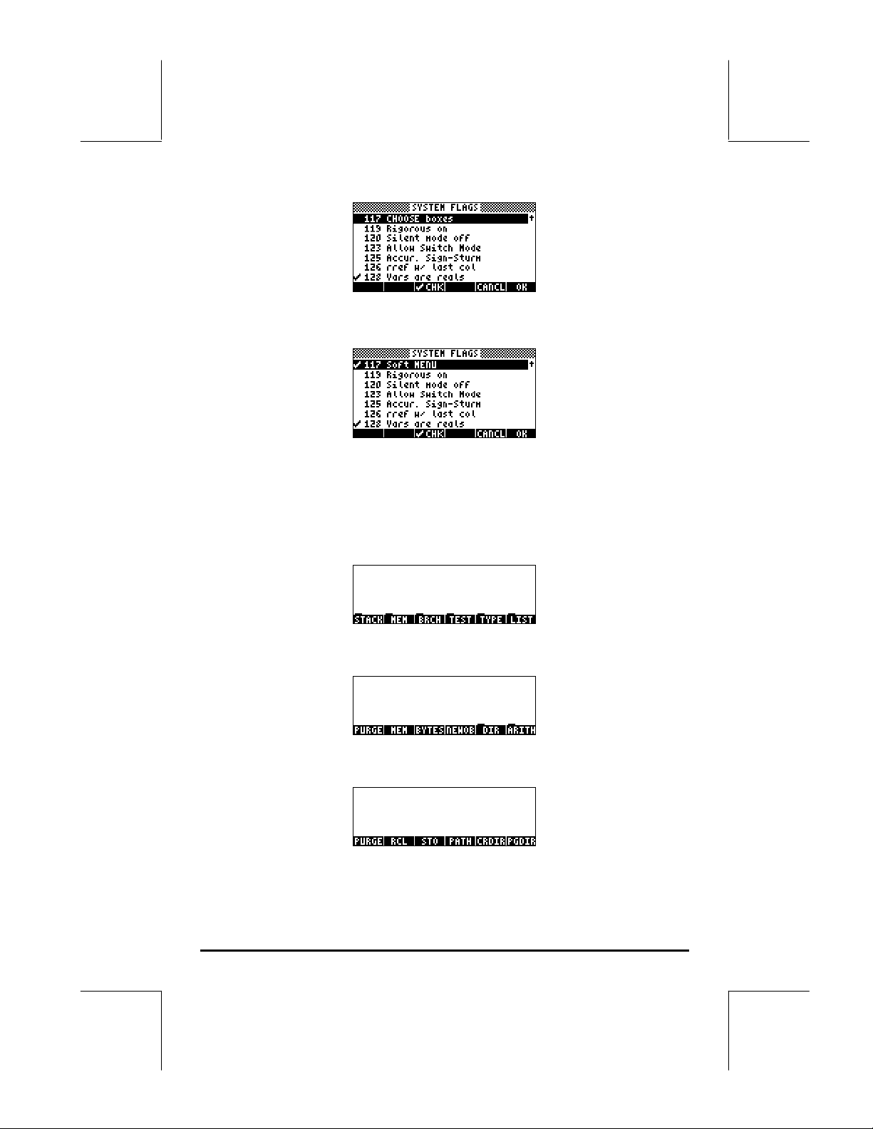
Now, we’ll try to find the ORDER command using similar keystrokes to those used above, i.e., we start with „°. Notice that instead of a menu list, we get soft menu labels with the different options in the PROG menu, i.e.,

Press B to select the MEMORY soft menu ()@@MEM@@). The display now shows:

Press E to select the DIRECTORY soft menu ()@@DIR@@)

Page 2-19

The ORDER command is not shown in this screen. To find it we use the L key to find it:

To activate the ORDER command we press the C(@ORDER) soft menu key.

References

For additional information on entering and manipulating expressions in the display or in the Equation Writer see Chapter 2 of the calculator’s user’s guide. For CAS (Computer Algebraic System) settings, see Appendix C in the calculator’s user’s guide. For information on Flags see, Chapter 24 in the calculator’s user’s guide.

Page 2-20

Chapter 3 Calculations with real numbers

This chapter demonstrates the use of the calculator for operations and functions related to real numbers. The user should be acquainted with the keyboard to identify certain functions available in the keyboard (e.g., SIN, COS, TAN, etc.). Also, it is assumed that the reader knows how to change the calculator’s operating system (Chapter 1), use menus and choose boxes (Chapter 1), and operate with variables (Chapter 2).

Examples of real number calculations

To perform real number calculations it is preferred to have the CAS set to Real (as opposed to Complex) mode. Exact mode is the default mode for most operations. Therefore, you may want to start your calculations in this mode. Some operations with real numbers are illustrated next:

• Use the \ key for changing sign of a number.

For example, in ALG mode, \2.5`. In RPN mode, e.g., 2.5\.

• Use the Ykey to calculate the inverse of a number.

For example, in ALG mode, Y2`. In RPN mode use 4`Y.

• For addition, subtraction, multiplication, division, use the proper

operation key, namely, + - * /.

Examples in ALG mode:

3.7 + 5.2 `

6.3 - 8.5 `

4.2 * 2.5 `

2.3 / 4.5 `

Examples in RPN mode:

3.7` 5.2 +

Page 3-1

6.3` 8.5 -

4.2` 2.5 *

2.3` 4.5 /

Alternatively, in RPN mode, you can separate the operands with a space (#) before pressing the operator key. Examples:

3.7#5.2 +

6.3#8.5 -

4.2#2.5 *

2.3#4.5 /

• Parentheses („Ü) can be used to group operations, as well as to enclose arguments of functions. In ALG mode:

„Ü5+3.2™/„Ü7-

2.2`

In RPN mode, you do not need the parenthesis, calculation is done directly on the stack:

5`3.2`+7`2.2`-/

In RPN mode, typing the expression between single quotes will allow you to enter the expression like in algebraic mode:

³„Ü5+3.2™/

„Ü7-2.2`µ

For both, ALG and RPN modes, using the Equation Writer:

‚O5+3.2™/7-2.2

The expression can be evaluated within the Equation writer, by using

————@EVAL@ or, ‚—@EVAL@

• The absolute value function, ABS, is available through „Ê. Example in ALG mode:

Page 3-2

„Ê \2.32`

Example in RPN mode:

2.32\„Ê

• The square function, SQ, is available through „º. Example in ALG mode:

„º\2.3`

Example in RPN mode:

2.3\„º

The square root function, √, is available through the R key. When calculating in the stack in ALG mode, enter the function before the argument, e.g.,

R123.4`

In RPN mode, enter the number first, then the function, e.g.,

123.4R

• The power function, ^, is available through the Q key. When calculating in the stack in ALG mode, enter the base (y) followed by the Q key, and then the exponent (x), e.g.,

5.2Q1.25`

In RPN mode, enter the number first, then the function, e.g.,

5.2`1.25Q

• The root function, XROOT(y,x), is available through the keystroke combination ‚». When calculating in the stack in ALG mode,

Page 3-3

enter the function XROOT followed by the arguments (y,x), separated by commas, e.g.,

‚»3‚í 27`

In RPN mode, enter the argument y, first, then, x, and finally the function call, e.g.,

27`3‚»

• Logarithms of base 10 are calculated by the keystroke combination ‚Ã (function LOG) while its inverse function (ALOG, or antilogarithm) is calculated by using „Â. In ALG mode, the function is entered before the argument:

‚Ã2.45` „Â\2.3`

In RPN mode, the argument is entered before the function

2.45 ‚Ã

2.3\ „Â

Using powers of 10 in entering data

Powers of ten, i.e., numbers of the form -4.5×10-2, etc., are entered by using the V key. For example, in ALG mode:

\4.5V\2`

Or, in RPN mode:

4.5\V2\`

• Natural logarithms are calculated by using ‚¹ (function LN) while the exponential function (EXP) is calculated by using „¸. In ALG mode, the function is entered before the argument:

‚¹2.45` „¸\2.3`

In RPN mode, the argument is entered before the function

Page 3-4

2.45` ‚¹

2.3\` „¸

• Three trigonometric functions are readily available in the keyboard: sine (S), cosine (T), and tangent (U). Arguments of these functions are angles in either degrees, radians, grades. The following examples use angles in degrees (DEG):

In ALG mode:

S30` T45`

U135`

In RPN mode:

30S 45T

135U

• The inverse trigonometric functions available in the keyboard are the arcsine („¼), arccosine („¾), and arctangent („À). The answer from these functions will be given in the selected angular measure (DEG, RAD, GRD). Some examples are shown next:

In ALG mode:

„¼0.25` „¾0.85` „À1.35`

In RPN mode:

0.25„¼

0.85„¾

1.35„À

All the functions described above, namely, ABS, SQ, √, ^, XROOT, LOG, ALOG, LN, EXP, SIN, COS, TAN, ASIN, ACOS, ATAN, can be combined with the fundamental operations (+-*/) to form more complex expressions. The Equation Writer, whose operations is described in Chapter 2, is ideal for building such expressions, regardless of the calculator operation mode.

Page 3-5

Real number functions in the MTH menu

The MTH („´) menu include a number of mathematical functions mostly applicable to real numbers. With the default setting of CHOOSE boxes for system flag 117 (see Chapter 2), the MTH menu shows the following functions:

The functions are grouped by the type of argument (1. vectors, 2. matrices, 3. lists, 7. probability, 9. complex) or by the type of function (4. hyperbolic, 5. real, 6. base, 8. fft). It also contains an entry for the mathematical constants available in the calculator, entry 10.

In general, be aware of the number and order of the arguments required for each function, and keep in mind that, in ALG mode you should select first the function and then enter the argument, while in RPN mode, you should enter the argument in the stack first, and then select the function.

Using calculator menus:

1. We will describe in detail the use of the 4. HYPERBOLIC.. menu in this

section with the intention of describing the general operation of calculator menus. Pay close attention to the process for selecting different options.

2. To quickly select one of the numbered options in a menu list (or CHOOSE box), simply press the number for the option in the keyboard. For example, to select option 4. HYPERBOLIC.. in the MTH menu, simply press 4.

Hyperbolic functions and their inverses

Selecting Option 4. HYPERBOLIC.. , in the MTH menu, and pressing @@OK@@, produces the hyperbolic function menu:

Page 3-6

For example, in ALG mode, the keystroke sequence to calculate, say, tanh(2.5), is the following:

„´4 @@OK@@ 5 @@OK@@ 2.5`

In the RPN mode, the keystrokes to perform this calculation are the following:

2.5`„´4 @@OK@@ 5 @@OK@@

The operations shown above assume that you are using the default setting for system flag 117 (CHOOSE boxes). If you have changed the setting of this flag (see Chapter 2) to SOFT menu, the MTH menu will show as follows (left-hand side in ALG mode, right –hand side in RPN mode):

Pressing L shows the remaining options:

Thus, to select, for example, the hyperbolic functions menu, with this menu format press )@@HYP@ , to produce:

Page 3-7

Finally, in order to select, for example, the hyperbolic tangent (tanh) function, simply press @@TANH@.

Note: To see additional options in these soft menus, press the L key or the „«keystroke sequence.

For example, to calculate tanh(2.5), in the ALG mode, when using SOFT menus over CHOOSE boxes, follow this procedure:

„´@@HYP@ @@TANH@ 2.5`

In RPN mode, the same value is calculated using:

2.5`„´)@@HYP@ @@TANH@

As an exercise of applications of hyperbolic functions, verify the following values:

SINH (2.5) = 6.05020.. ASINH(2.0) = 1.4436… COSH (2.5) = 6.13228.. ACOSH (2.0) = 1.3169… TANH(2.5) = 0.98661.. ATANH(0.2) = 0.2027… EXPM(2.0) = 6.38905…. LNP1(1.0) = 0.69314….

Operations with units

Numbers in the calculator can have units associated with them. Thus, it is possible to calculate results involving a consistent system of units and produce a result with the appropriate combination of units.

The UNITS menu

The units menu is launched by the keystroke combination ‚Û(associated with the 6 key). With system flag 117 set to CHOOSE boxes, the result is the following menu:

Page 3-8

Option 1. Tools.. contains functions used to operate on units (discussed later). Options 2. Length.. through 17.Viscosity.. contain menus with a number of units for each of the quantities described. For example, selecting option 8. Force.. shows the following units menu:

The user will recognize most of these units (some, e.g., dyne, are not used very often nowadays) from his or her physics classes: N = newtons, dyn = dynes, gf = grams – force (to distinguish from gram-mass, or plainly gram, a unit of mass), kip = kilo-poundal (1000 pounds), lbf = pound-force (to distinguish from pound-mass), pdl = poundal.

To attach a unit object to a number, the number must be followed by an underscore. Thus, a force of 5 N will be entered as 5_N.

For extensive operations with units SOFT menus provide a more convenient way of attaching units. Change system flag 117 to SOFT menus (see Chapter 2), and use the keystroke combination ‚Û to get the following menus. Press L to move to the next menu page.

Page 3-9

Pressing on the appropriate soft menu key will open the sub-menu of units for that particular selection. For example, for the @)SPEED sub-menu, the following units are available:

Pressing the soft menu key @)UNITS will take you back to the UNITS menu.

Recall that you can always list the full menu labels in the screen by using ‚˜, e.g., for the @)ENRG set of units the following labels will be listed:

Note: Use the L key or the „«keystroke sequence to navigate through the menus.

Available units

For a complete list of available units see Chapter 3 in the calculator’s user’s guide.

Page 3-10

Attaching units to numbers

To attach a unit object to a number, the number must be followed by an underscore (‚Ý, key(8,5)). Thus, a force of 5 N will be entered as 5_N.

Here is the sequence of steps to enter this number in ALG mode, system flag 117 set to CHOOSE boxes:

Note: If you forget the underscore, the result is the expression 5*N, where N here represents a possible variable name and not Newtons.

To enter this same quantity, with the calculator in RPN mode, use the following keystrokes:

Notice that the underscore is entered automatically when the RPN mode is active.

The keystroke sequences to enter units when the SOFT menu option is selected, in both ALG and RPN modes, are illustrated next. For example, in ALG mode, to enter the quantity 5_N use:

The same quantity, entered in RPN mode uses the following keystrokes:

Note: You can enter a quantity with units by typing the underline and units with the ~keyboard, e.g., 5‚Ý~n will produce the entry: 5_N

Unit prefixes

You can enter prefixes for units according to the following table of prefixes from the SI system. The prefix abbreviation is shown first, followed by its name, and by the exponent x in the factor 10

5‚Ý ‚Û 8@@OK@@ @@OK@@ `

5‚Û8@@OK@@ @@OK@@

5‚Ý ‚ÛL @)@FORCE @ @@N@@ `

5‚ÛL @)@FORCE @ @@N@@

corresponding to each prefix:

Page 3-11

____________________________________________________ Prefix Name x Prefix Name x ____________________________________________________ Y yotta +24 d deci -1 Z zetta +21 c centi -2 E exa +18 m milli -3 P peta +15 µ micro -6 T tera +12 n nano -9 G giga +9 p pico -12 M mega +6 f femto -15 k,K kilo +3 a atto -18 h,H hecto +2 z zepto -21 D(*) deka +1 y yocto -24 _____________________________________________________

(*) In the SI system, this prefix is da rather than D. Use D for deka in the calculator, however.

To enter these prefixes, simply type the prefix using the ~ keyboard. For example, to enter 123 pm (picometer), use:

123‚Ý~„p~„m

Using UBASE (type the name) to convert to the default unit (1 m) results in:

Operations with units

Here are some calculation examples using the ALG operating mode. Be warned that, when multiplying or dividing quantities with units, you must enclosed each quantity with its units between parentheses. Thus, to enter, for example, the product 12.5m × 5.2 yd, type it to read (12.5_m)*(5.2_yd) `:

Page 3-12

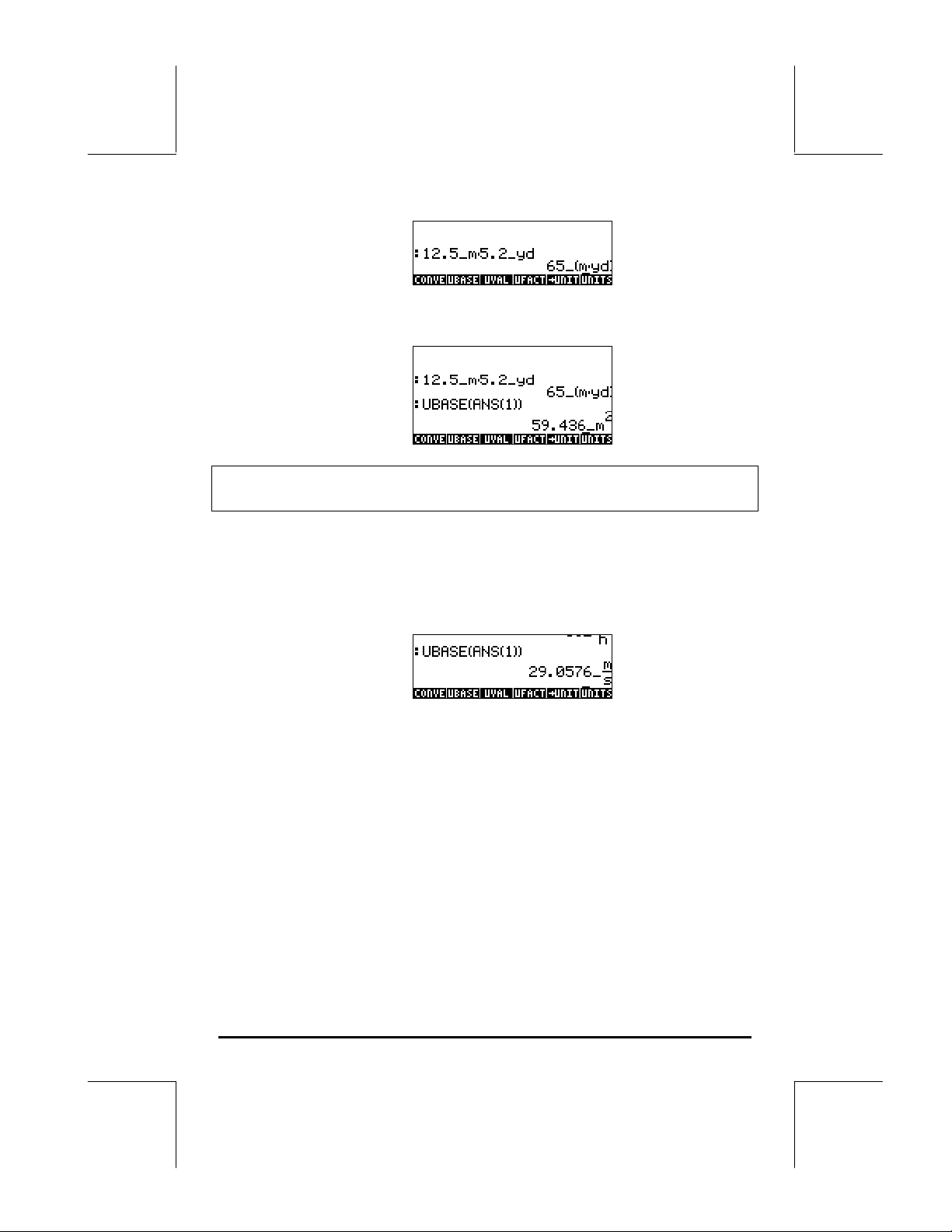
which shows as 65_(m⋅yd). To convert to units of the SI system, use function UBASE (find it using the command catalog, ‚N):

Note: Recall that the ANS(1) variable is available through the keystroke combination „î(associated with the ` key).

To calculate a division, say, 3250 mi / 50 h, enter it as

(3250_mi)/(50_h) `

which transformed to SI units, with function UBASE, produces:

Addition and subtraction can be performed, in ALG mode, without using parentheses, e.g., 5 m + 3200 mm, can be entered simply as

5_m + 3200_mm `.

More complicated expression require the use of parentheses, e.g.,

(12_mm)*(1_cm^2)/(2_s) `:

Stack calculations in the RPN mode, do not require you to enclose the different terms in parentheses, e.g.,

12 @@@m@@@ 1.5 @@yd@@ *

3250 @@mi@@ 50 @@@h@@@ /

Page 3-13

These operations produce the following output:

Unit conversions

The UNITS menu contains a TOOLS sub-menu, which provides the following functions:

CONVERT(x,y): convert unit object x to units of object y UBASE(x): convert unit object x to SI units UVAL(x): extract the value from unit object x UFACT(x,y): factors a unit y from unit object x UNIT(x,y): combines value of x with units of y

Examples of function CONVERT are shown below. Examples of the other UNIT/TOOLS functions are available in Chapter 3 of the calculator’s user’s guide. For example, to convert 33 watts to btu’s use either of the following entries:

CONVERT(33_W,1_hp) `

CONVERT(33_W,11_hp) `

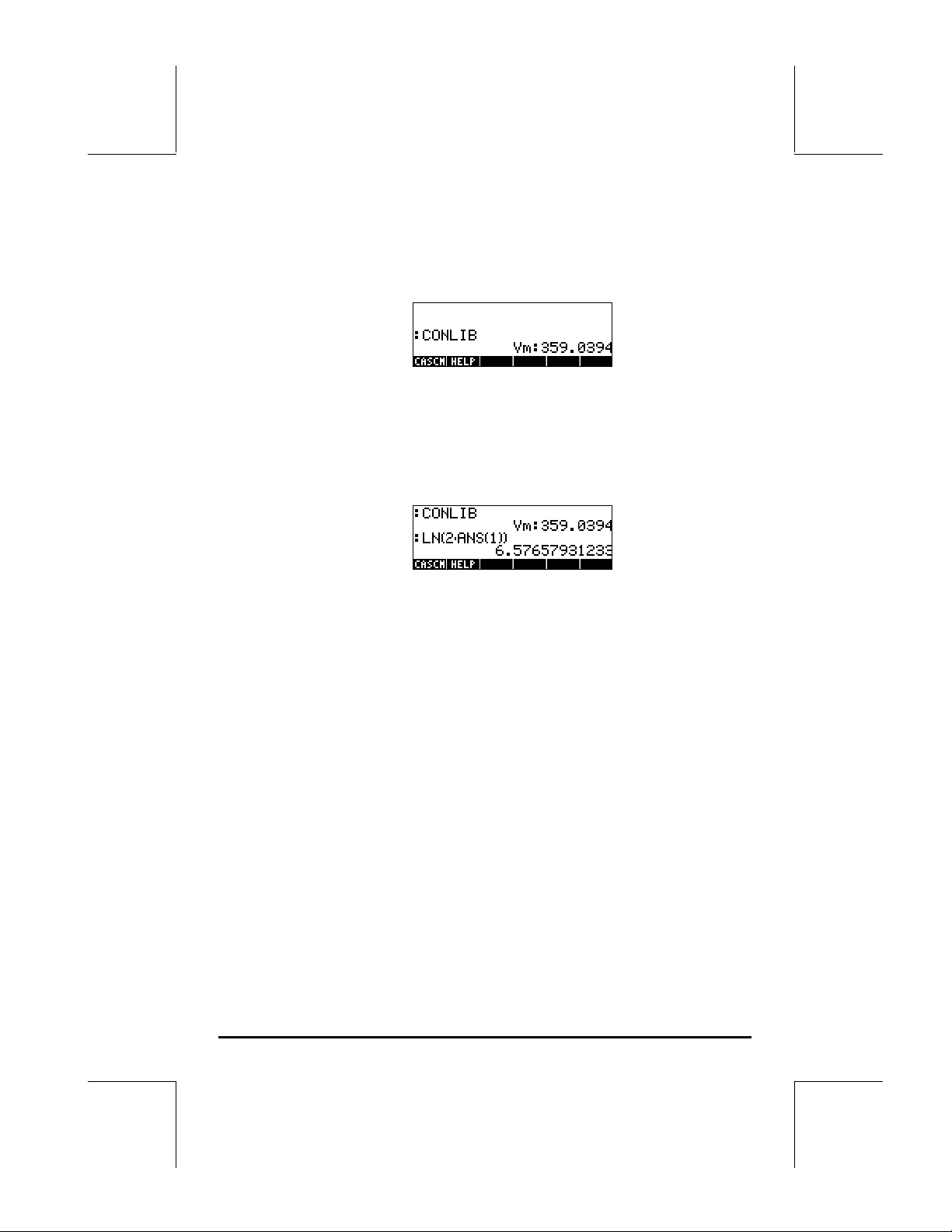
Physical constants in the calculator

The calculator’s physical constants are contained in a constants library activated with the command CONLIB. To launch this command you could simply type it in the stack: ~~conlib`, or, you can select the command CONLIB from the command catalog, as follows: First, launch the catalog by using: ‚N~c. Next, use the up and down arrow keys —˜ to select CONLIB. Finally, press the F(@@OK@@) soft menu key. Press `, if needed. Use the up and down arrow keys (—˜) to navigate through the list of constants in your calculator.

Page 3-14

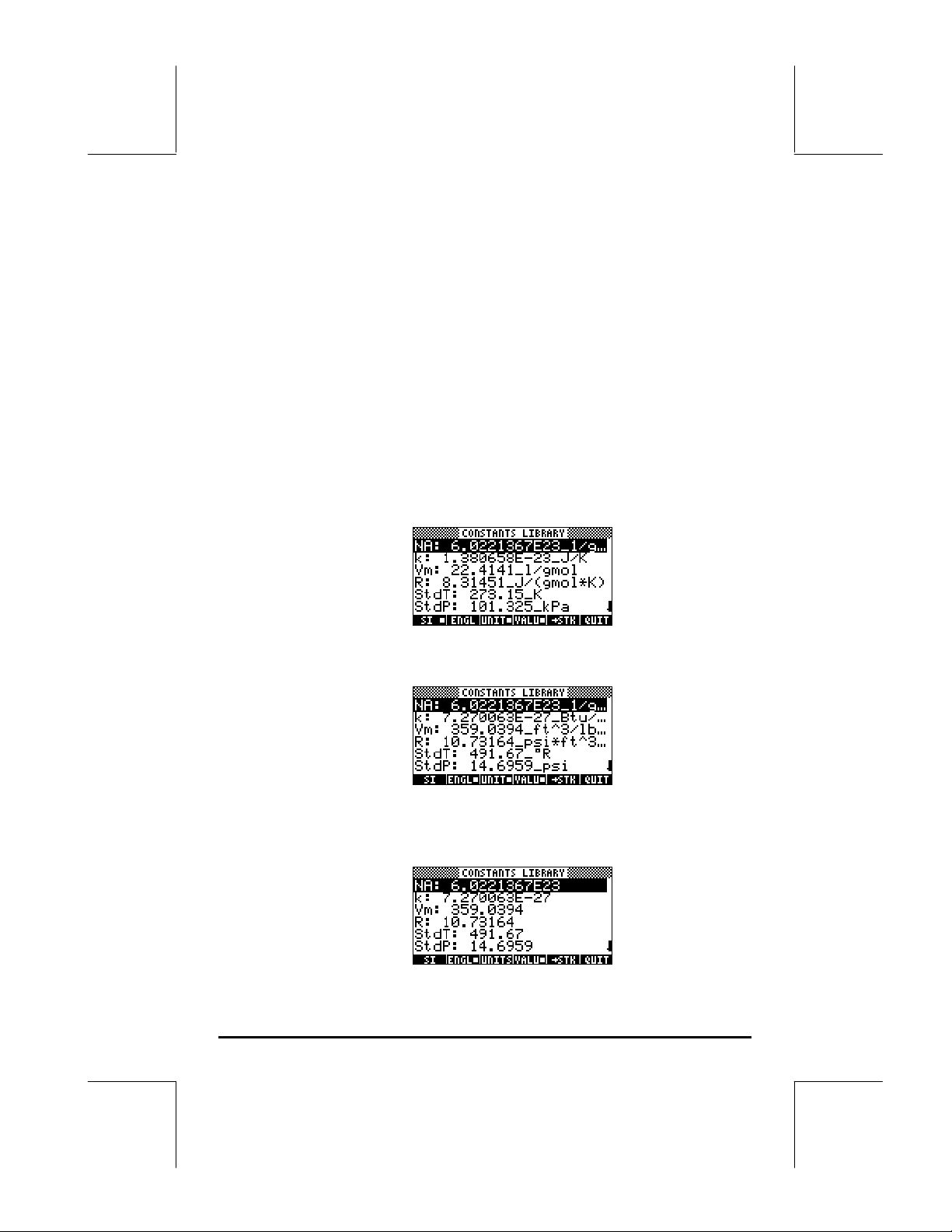
The soft menu keys corresponding to this CONSTANTS LIBRARY screen include the following functions:

SI when selected, constants values are shown in SI units (*) ENGL when selected, constants values are shown in English units (*) UNIT when selected, constants are shown with units attached (*) VALUE when selected, constants are shown without units STK copies value (with or without units) to the stack QUIT exit constants library

(*) Activated only if the VALUE option is selected.

This is the way the top of the CONSTANTS LIBRARY screen looks when the option VALUE is selected (units in the SI system):

To see the values of the constants in the English (or Imperial) system, press the @ENGL option:

If we de-select the UNITS option (press @UNITS ) only the values are shown (English units selected in this case):

Page 3-15

To copy the value of Vm to the stack, select the variable name, and press !²STK, then, press @QUIT@. For the calculator set to the ALG, the screen will look like this:

The display shows what is called a tagged value, Vm:359.0394. In here, Vm, is the tag of this result. Any arithmetic operation with this number will ignore the tag. Try, for example:

‚¹2*„î `

which produces:

The same operation in RPN mode will require the following keystrokes (after the value of Vm was extracted from the constants library):

2`*‚¹

Defining and using functions

Users can define their own functions by using the DEFINE command available thought the keystroke sequence „à (associated with the 2 key). The function must be entered in the following format:

Function_name(arguments) = expression_containing_arguments

For example, we could define a simple function

H(x) = ln(x+1) + exp(-x)

Suppose that you have a need to evaluate this function for a number of discrete values and, therefore, you want to be able to press a single button

Page 3-16

and get the result you want without having to type the expression in the righthand side for each separate value. In the following example, we assume you have set your calculator to ALG mode. Enter the following sequence of keystrokes:

„à³~h„Ü~„x™‚Å

‚¹~„x+1™+„¸~„x`

The screen will look like this:

Press the J key, and you will notice that there is a new variable in your soft menu key (@@@H@@). To see the contents of this variable press ‚@@@H@@. The screen will show now:

Thus, the variable H contains a program defined by:

<<  x ‘LN(x+1) + EXP(x)’ >>

This is a simple program in the default programming language of the HP 48 G series, and also incorporated in the HP 49 G series. This programming language is called UserRPL (See Chapters 20 and 21 in the calculator’s user’s guide). The program shown above is relatively simple and consists of two parts, contained between the program containers << >>:

• Input:  x  x

• Process: ‘LN(x+1) + EXP(x) ‘

This is to be interpreted as saying: enter a value that is temporarily assigned to the name x (referred to as a local variable), evaluate the expression

Page 3-17

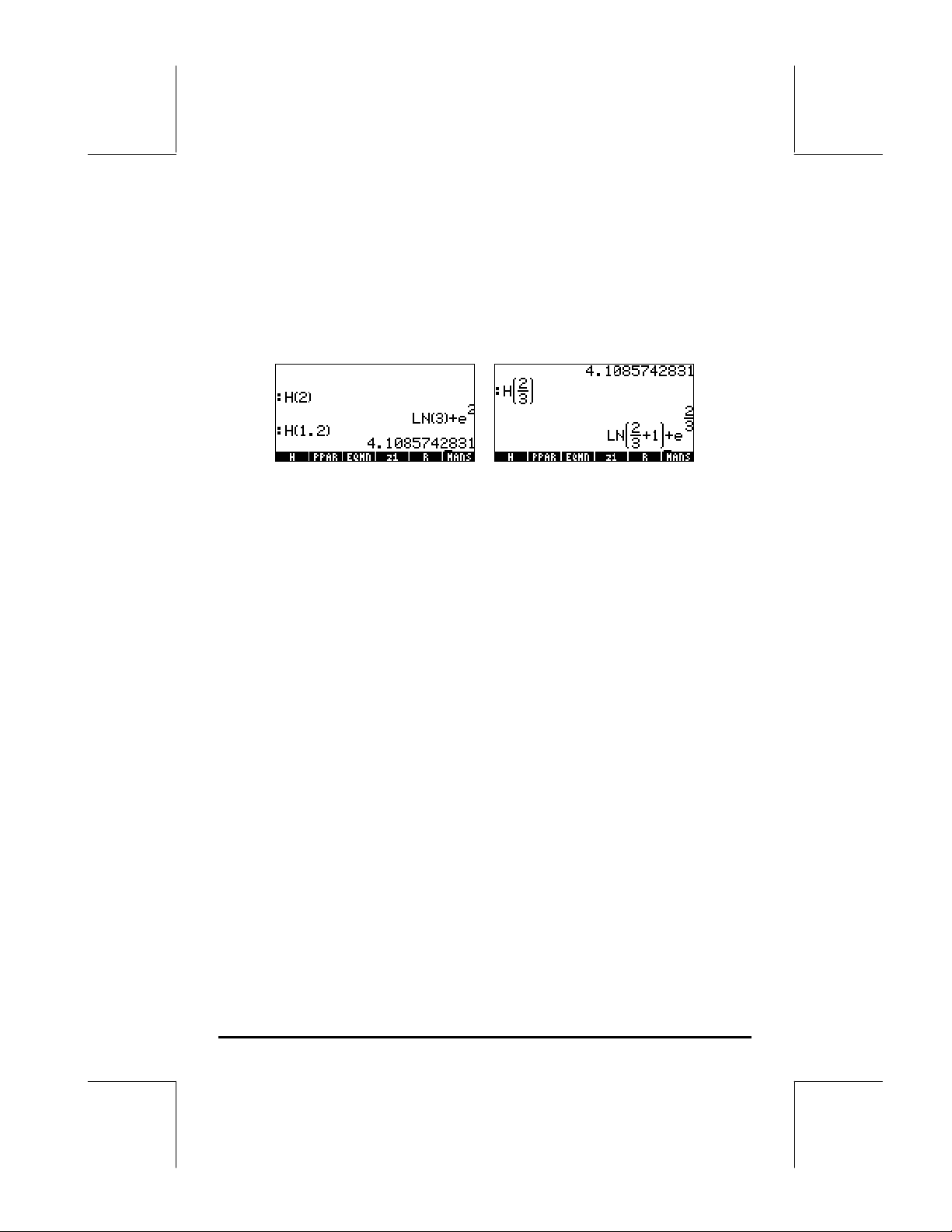
between quotes that contain that local variable, and show the evaluated expression.

To activate the function in ALG mode, type the name of the function followed by the argument between parentheses, e.g., @@@H@@@ „Ü2`. Some examples are shown below:

In the RPN mode, to activate the function enter the argument first, then press the soft menu key corresponding to the variable name @@@H@@@ . For example, you could try: 2`@@@H@@@ . The other examples shown above can be entered by using: 1.2`@@@H@@@ , 2`3/@@@H@@@.

Reference

Additional information on operations with real numbers with the calculator is contained in Chapter 3 of the user’s guide.

Page 3-18

Chapter 4 Calculations with complex numbers

This chapter shows examples of calculations and application of functions to complex numbers.

Definitions

A complex number z is written as z = x + iy, (Cartesian form) where x and y are real numbers, and i is the imaginary unit defined by i has a real part, x = Re(z), and an imaginary part, y = Im(z). The polar form

of a complex number is z = re

yx + is the modulus of the complex number z, and θ = Arg(z) =

= r⋅cosθ + i r⋅sinθ, where r = |z|

arctan(y/x) is the argument of the complex number z. The complex conjugate

of a complex number z = x + iy = re

z, –z = -x-iy = - re

, can be thought of as the reflection of z about the origin.

, isz = x – iy = re

= -1. The number

-i

. The negative of

Setting the calculator to COMPLEX mode

To work with complex numbers select the CAS complex mode:

H)@@CAS@ ˜˜™@@CHK

The COMPLEX mode will be selected if the CAS MODES screen shows the option _Complex checked off, i.e.,

Press @@OK@@ , twice, to return to the stack.

Page 4-1

Entering complex numbers

Complex numbers in the calculator can be entered in either of the two Cartesian representations, namely, x+iy, or (x,y). The results in the calculator will be shown in the ordered-pair format, i.e., (x,y). For example, with the calculator in ALG mode, the complex number (3.5,-1.2), is entered as:

„Ü3.5‚í\1.2`

A complex number can also be entered in the form x+iy. For example, in ALG mode, 3.5-1.2i is entered as (accept mode changes):

3.5 -1.2*„„¥`

In RPN mode, these numbers could be entered using the following keystrokes:

„Ü3.5‚í1.2\`

(Notice that the change-sign keystroke is entered after the number 1.2 has been entered, in the opposite order as the ALG mode exercise), and

³3.5 -1.2*„„¥`

(Notice the need to enter an apostrophe before typing the number 3.5-1.2i in RPN mode).

To enter the unit imaginary number alone type : „¥(the I key).

Polar representation of a complex number

The polar representation of the complex number 3.5-1.2i, entered above, is obtained by changing the coordinate system to cylindrical or polar (using function CYLIN). You can find this function in the catalog (‚N). You can also change the coordinate to POLAR using H. Changing to polar coordinate with the angular measure in radians, produces the result:

Page 4-2

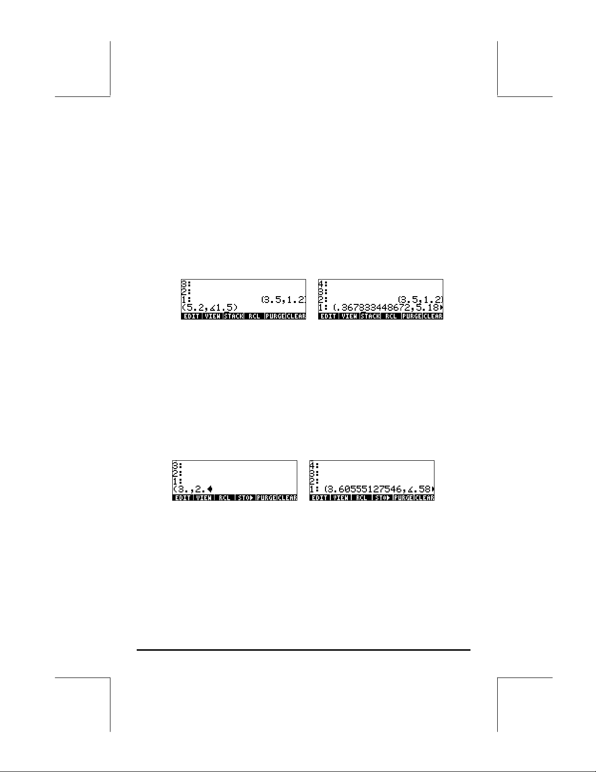
The result shown above represents a magnitude, 3.7, and an angle

0.33029…. The angle symbol (∠) is shown in front of the angle measure.

Return to Cartesian or rectangular coordinates by using function RECT (available in the catalog, ‚N). A complex number in polar

representation is written as z = r⋅e

. You can enter this complex number into the calculator by using an ordered pair of the form (r, ∠θ). The angle symbol (∠) can be entered as ~‚6. For example, the complex number z =

1.5i

5.2e

, can be entered as follows (the figures show the RPN stack, before

and after entering the number):

Because the coordinate system is set to rectangular (or Cartesian), the calculator automatically converts the number entered to Cartesian coordinates, i.e., x = r cos θ, y = r sin θ, resulting, for this case, in (0.3678…, 5.18…).

On the other hand, if the coordinate system is set to cylindrical coordinates (use CYLIN), entering a complex number (x,y), where x and y are real numbers, will produce a polar representation. For example, in cylindrical coordinates, enter the number (3.,2.). The figure below shows the RPN stack, before and after entering this number:

Simple operations with complex numbers

Complex numbers can be combined using the four fundamental operations (+-*/). The results follow the rules of algebra with the caveat that

= -1. Operations with complex numbers are similar to those with real

numbers. For example, with the calculator in ALG mode and the CAS set to Complex, try the following operations:

Page 4-3

(3+5i) + (6-3i) = (9,2);

(5-2i) - (3+4i) = (2,-6)

(3-i)(2-4i) = (2,-14);

(5-2i)/(3+4i) = (0.28,-1.04)

1/(3+4i) = (0.12, -0.16) ;

-(5-3i) = -5 + 3i

The CMPLX menus

There are two CMPLX (CoMPLeX numbers) menus available in the calculator. One is available through the MTH menu (introduced in Chapter 3) and one directly into the keyboard (‚ß). The two CMPLX menus are presented next.

CMPLX menu through the MTH menu

Assuming that system flag 117 is set to CHOOSE boxes (see Chapter 2), the CMPLX sub-menu within the MTH menu is accessed by using: „´9 @@OK@@ . The functions available are the following:

The first menu (options 1 through 6) shows the following functions: RE(z) : Real part of a complex number IM(z) : Imaginary part of a complex number

C→R(z) : Separates a complex number into its real and imaginary parts R→C(x,y) : Forms the complex number (x,y) out of real numbers x and y

ABS(z) : Calculates the magnitude of a complex number. ARG(z) : Calculates the argument of a complex number. SIGN(z) : Calculates a complex number of unit magnitude as z/|z|. NEG(z) : Changes the sign of z CONJ(z) : Produces the complex conjugate of z

Page 4-4

Examples of applications of these functions are shown next in RECT coordinates. Recall that, for ALG mode, the function must precede the argument, while in RPN mode, you enter the argument first, and then select the function. Also, recall that you can get these functions as soft menu labels by changing the setting of system flag 117 (See Chapter 2).

CMPLX menu in keyboard

A second CMPLX menu is accessible by using the right-shift option associated with the 1 key, i.e., ‚ß. With system flag 117 set to CHOOSE boxes, the keyboard CMPLX menu shows up as the following screens:

The resulting menu include some of the functions already introduced in the previous section, namely, ARG, ABS, CONJ, IM, NEG, RE, and SIGN. It also includes function i which serves the same purpose as the keystroke combination „¥.

Page 4-5

Functions applied to complex numbers

Many of the keyboard-based functions and MTH menu functions defined in Chapter 3 for real numbers (e.g., SQ, ,LN, e complex numbers. The result is another complex number, as illustrated in the following examples.

, etc.), can be applied to

Note: When using trigonometric functions and their inverses with complex numbers the arguments are no longer angles. Therefore, the angular measure selected for the calculator has no bearing in the calculation of these functions with complex arguments.

Function DROITE: equation of a straight line

Function DROITE takes as argument two complex numbers, say, x1+iy1 and x

+iy2, and returns the equation of the straight line, say, y = a+bx, that

contains the points (x A(5,-3) and B(6,2) can be found as follows (example in Algebraic mode):

) and (x2,y2). For example, the line between points

1,y1

Page 4-6

Function DROITE is found in the command catalog (‚N). If the calculator is in APPROX mode, the result will be Y = 5.*(X-5.)-3.

Reference

Additional information on complex number operations is presented in Chapter 4 of the calculator’s user’s guide.

Page 4-7

Chapter 5 Algebraic and arithmetic operations

An algebraic object, or simply, algebraic, is any number, variable name or algebraic expression that can be operated upon, manipulated, and combined according to the rules of algebra. Examples of algebraic objects are the following:

• A number: 12.3, 15.2_m, ‘π’, ‘e’, ‘i’

• A variable name: ‘a’, ‘ux’, ‘width’, etc.

• An expression: ‘p*D^2/4’,’f*(L/D)*(V^2/(2*g))’,

• An equation: ‘p*V = n*R*T’, ‘Q=(Cu/n)*A(y)*R(y)^(2/3)*√So’

Entering algebraic objects

Algebraic objects can be created by typing the object between single quotes directly into stack level 1 or by using the equation writer [EQW]. For example, to enter the algebraic object ‘π*D^2/4’ directly into stack level 1 use:

³„ì*~dQ2/4`

An algebraic object can also be built in the Equation Writer and then sent to the stack, or operated upon in the Equation Writer itself. The operation of the Equation Writer was described in Chapter 2. As an exercise, build the following algebraic object in the Equation Writer:

Page 5-1

After building the object, press ` to show it in the stack (ALG and RPN modes shown below):

Simple operations with algebraic objects

Algebraic objects can be added, subtracted, multiplied, divided (except by zero), raised to a power, used as arguments for a variety of standard functions (exponential, logarithmic, trigonometry, hyperbolic, etc.), as you would any real or complex number. To demonstrate basic operations with algebraic objects, let’s create a couple of objects, say ‘π*R^2’ and ‘g*t^2/4’, and store them in variables A1 and A2 (See Chapter 2 to learn how to create variables and store values in them). Here are the keystrokes for storing variables A1 in ALG mode:

³„ì*~rQ2™ K ~a1 `

resulting in:

The keystrokes corresponding to RPN mode are:

„ì~r`2Qx ~a1 K

After storing the variable A2 and pressing the key, the screen will show the variables as follows:

Page 5-2

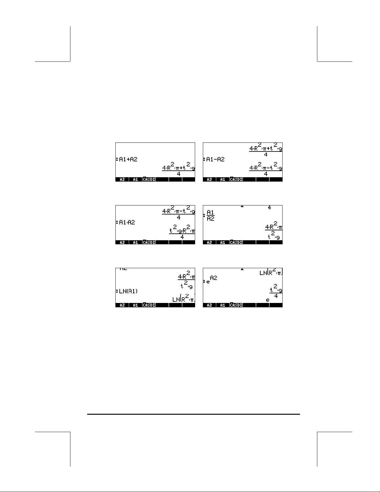
In ALG mode, the following keystrokes will show a number of operations with the algebraics contained in variables @@A1@@ and @@A2@@ (press J to recover variable menu):

@@A1@@ + @@A2@@ ` @@A1@@ - @@A2@@ `

@@A1@@ * @@A2@@ ` @@A1@@ / @@A2@@ `

‚¹@@A1@@ „¸@@A2@@

The same results are obtained in RPN mode if using the following keystrokes:

@@A1@ ` @@A2@@ + @@A1@@ ` @@A2@@ -

@@A1@@ ` @@A2@@ * @@A1@@ ` @@A2@@ /

@@A1@@ ` ‚¹ @@A2@@ ` „¸

Page 5-3

Functions in the ALG menu

The ALG (Algebraic) menu is available by using the keystroke sequence ‚× (associated with the 4 key). With system flag 117 set to CHOOSE boxes, the ALG menu shows the following functions:

Rather than listing the description of each function in this manual, the user is invited to look up the description using the calculator’s help facility: I L @)HELP@ ` . To locate a particular function, type the first letter of the function. For example, for function COLLECT, we type ~c, then use the up and down arrow keys, —˜, to locate COLLECT within the help window.

To complete the operation press @@OK@@. Here is the help screen for function COLLECT:

We notice that, at the bottom of the screen, the line See: EXPAND FACTOR suggests links to other help facility entries, the functions EXPAND and FACTOR. To move directly to those entries, press the soft menu key @SEE1! for EXPAND, and @SEE2! for FACTOR. Pressing @SEE1!, for example, shows the following information for EXPAND, while @SEE2! shows information for FACTOR:

Page 5-4

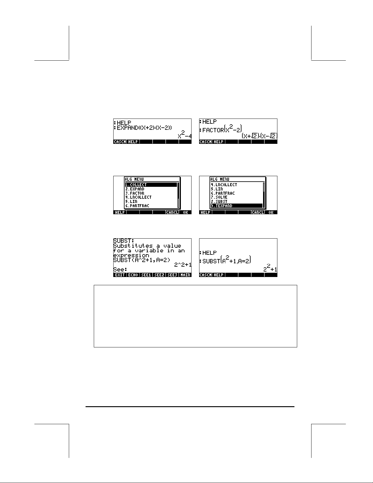
Copy the examples provided onto your stack by pressing @ECHO!. For example, for the EXPAND entry shown above, press the @ECHO! soft menu key to get the following example copied to the stack (press ` to execute the command):

Thus, we leave for the user to explore the applications of the functions in the ALG menu. This is a list of the commands:

For example, for function SUBST, we find the following CAS help facility entry:

Note: Recall that, to use these, or any other functions in the RPN mode, you must enter the argument first, and then the function. For example, the example for TEXPAND, in RPN mode will be set up as:

³„¸+~x+~y`

At this point, select function TEXPAND from menu ALG (or directly from the catalog ‚N), to complete the operation.

Page 5-5

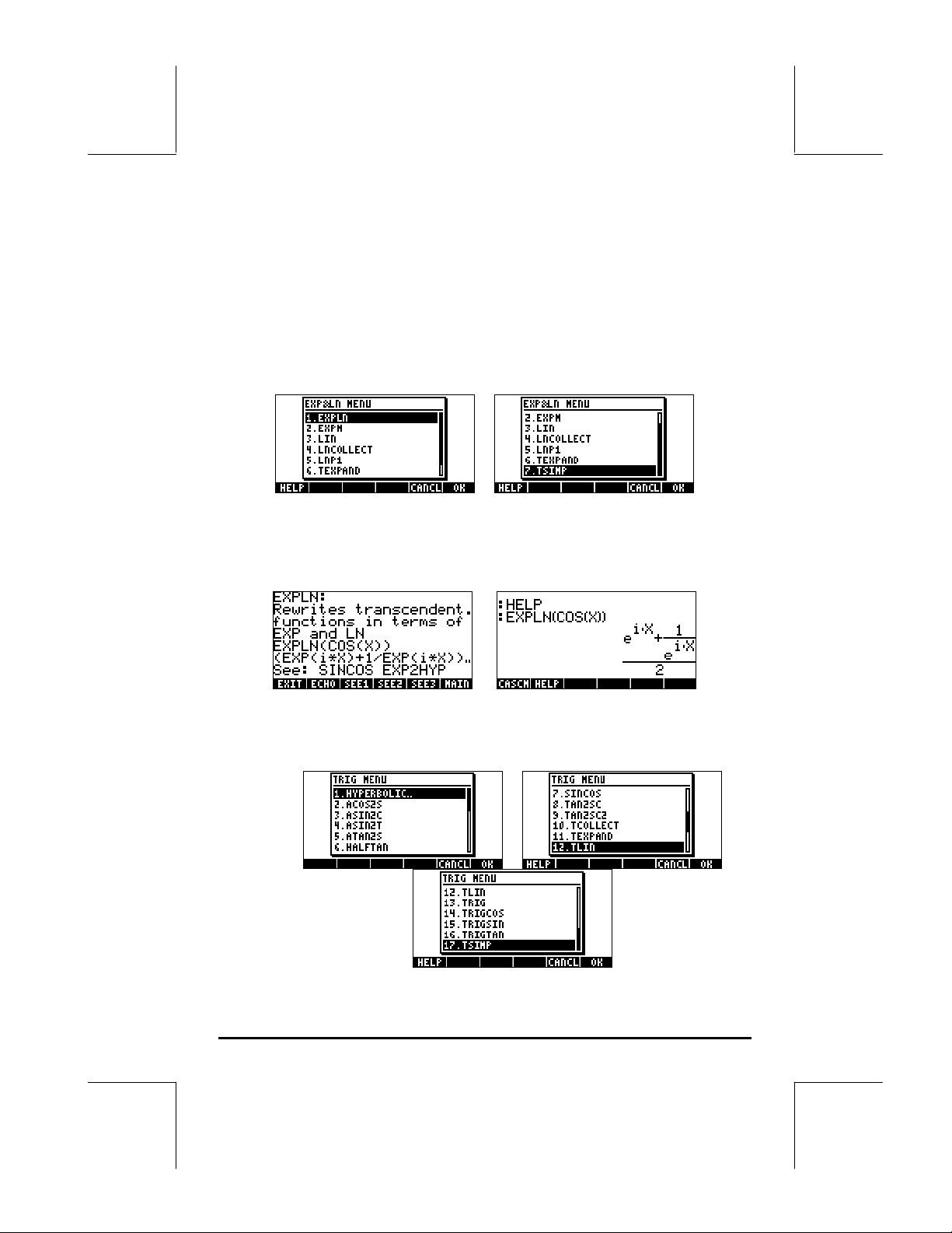
Operations with transcendental functions

The calculator offers a number of functions that can be used to replace expressions containing logarithmic and exponential functions („Ð), as well as trigonometric functions (‚Ñ).

Expansion and factoring using log-exp functions

The „Ð produces the following menu:

Information and examples on these commands are available in the help facility of the calculator. For example, the description of EXPLN is shown in the left-hand side, and the example from the help facility is shown to the right:

Expansion and factoring using trigonometric functions

The TRIG menu, triggered by using ‚Ñ, shows the following functions:

Page 5-6

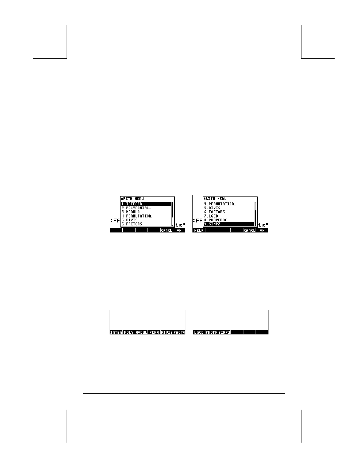
These functions allow to simplify expressions by replacing some category of trigonometric functions for another one. For example, the function ACOS2S allows to replace the function arccosine (acos(x)) with its expression in terms of arcsine (asin(x)).

Description of these commands and examples of their applications are available in the calculator’s help facility (IL@HELP). The user is invited to explore this facility to find information on the commands in the TRIG menu.

Functions in the ARITHMETIC menu

The ARITHMETIC menu is triggered through the keystroke combination „Þ (associated with the 1 key). With system flag 117 set to CHOOSE boxes, „Þ shows the following menu:

Out of this menu list, options 5 through 9 (DIVIS, FACTORS, LGCD, PROPFRAC, SIMP2) correspond to common functions that apply to integer numbers or to polynomials. The remaining options (1. INTEGER, 2. POLYNOMIAL, 3. MODULO, and 4. PERMUTATION) are actually submenus of functions that apply to specific mathematical objects. When system flag 117 is set to SOFT menus, the ARITHMETIC menu („Þ) produces:

Following, we present the help facility entries for functions FACTORS and SIMP2 in the ARITHMETIC menu:

Page 5-7

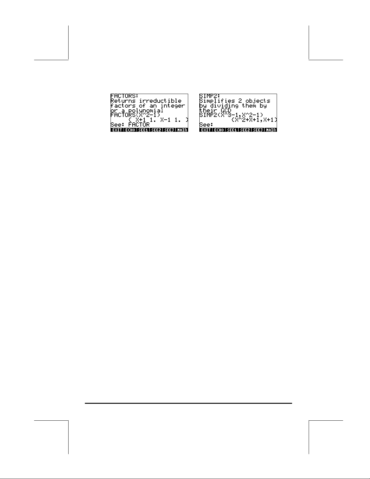
FACTORS: SIMP2:

The functions associated with the ARITHMETIC submenus: INTEGER, POLYNOMIAL, MODULO, and PERMUTATION, are presented in detail in Chapter 5 in the calculator’s user’s guide. The following sections show some applications to polynomials and fractions.

Polynomials

Polynomials are algebraic expressions consisting of one or more terms containing decreasing powers of a given variable. For example, ‘X^3+2*X^2-3*X+2’ is a third-order polynomial in X, while ‘SIN(X)^2-2’ is a second-order polynomial in SIN(X). Functions COLLECT and EXPAND, shown earlier, can be used on polynomials. Other applications of polynomial functions are presented next:

The HORNER function

The function HORNER („Þ, POLYNOMIAL, HORNER) produces the Horner division, or synthetic division, of a polynomial P(X) by the factor (X-a), i.e., HORNER(P(X),a) = {Q(X), a, P(a)}, where P(X) = Q(X)(X-a)+P(a). For example,

HORNER(‘X^3+2*X^2-3*X+1’,2) = {X^2+4*X+5 2 11}

i.e., X

+2X2-3X+1 = (X2+4X+5)(X-2)+11. Also,

HORNER(‘X^6-1’,-5)=

{ X^5-5*X^4+25*X^3-125*X^2+625*X-3125 -5 15624}

-1 = (X5-5*X4+25X3-125X2+625X-3125)(X+5)+15624.

Page 5-8

The variable VX

Most polynomial examples above were written using variable X. This is because a variable called VX exists in the calculator’s {HOME CASDIR} directory that takes, by default, the value of ‘X’. This is the name of the preferred independent variable for algebraic and calculus applications. Avoid using the variable VX in your programs or equations, so as to not get it confused with the CAS’ VX. For additional information on the CAS variable see Appendix C in the calculator’s user’s guide.

The PCOEF function

Given an array containing the roots of a polynomial, the function PCOEF generates an array containing the coefficients of the corresponding polynomial. The coefficients correspond to decreasing order of the independent variable. For example:

PCOEF([-2, –1, 0 ,1, 1, 2]) = [1. –1. –5. 5. 4. –4. 0.],

which represents the polynomial X

6-X5

-5X4+5X3+4X2-4X.

The PROOT function

Given an array containing the coefficients of a polynomial, in decreasing order, the function PROOT provides the roots of the polynomial. Example,

from X

+5X+6 =0, PROOT([1, –5, 6]) = [2. 3.].

The QUOT and REMAINDER functions

The functions QUOT and REMAINDER provide, respectively, the quotient Q(X) and the remainder R(X), resulting from dividing two polynomials, P P

(X). In other words, they provide the values of Q(X) and R(X) from

(X)/P2(X) = Q(X) + R(X)/P2(X). For example,

QUOT(‘X^3-2*X+2’, ‘X-1’) = ‘X^2+X-1’

REMAINDER(‘X^3-2*X+2’, ‘X-1’) = 1.

Thus, we can write: (X

-2X+2)/(X-1) = X2+X-1 + 1/(X-1).

(X) and

Page 5-9

Note: you could get the latter result by using PARTFRAC:

PARTFRAC(‘(X^3-2*X+2)/(X-1)’) = ‘X^2+X-1 + 1/(X-1)’.

The PEVAL function

The function PEVAL (Polynomial EVALuation) can be used to evaluate a polynomial

p(x) = a

⋅xn+a

given an array of coefficients [a result is the evaluation p(x

). Function PEVAL is not available in the

ARITHMETIC menu, instead use the CALC/DERIV&INTEG Menu. Example: PEVAL([1,5,6,1],5) = 281.

Additional applications of polynomial functions are presented in Chapter 5 in the calculator’s user’s guide.

n-1

⋅x

+ …+ a2⋅x2+a1⋅x+ a0,

n-1

, a

, … a2, a1, a0] and a value of x0. The

n-1

Fractions

Fractions can be expanded and factored by using functions EXPAND and FACTOR, from the ALG menu (‚×). For example:

EXPAND(‘(1+X)^3/((X-1)* (X+3))’) = ‘(X^3+3*X^2+3*X+1)/(X^2+2*X-3)’ EXPAND(‘(X^2*(X+Y)/(2*X-X^2)^2’) = ‘(X+Y)/(X^2-4*X+4)’

FACTOR(‘(3*X^3-2*X^2)/(X^2-5*X+6)’) = ‘X^2*(3*X-2)/((X-2)*(X-3))’ FACTOR(‘(X^3-9*X)/(X^2-5*X+6)’ ) = ‘X*(X+3)/(X-2)’

The SIMP2 function

Function SIMP2, in the ARITHMETIC menu, takes as arguments two numbers or polynomials, representing the numerator and denominator of a rational fraction, and returns the simplified numerator and denominator. For example:

SIMP2(‘X^3-1’,’X^2-4*X+3’) = { ‘X^2+X+1’,‘X-3’}

Page 5-10

The PROPFRAC function

The function PROPFRAC converts a rational fraction into a “proper” fraction, i.e., an integer part added to a fractional part, if such decomposition is possible. For example:

PROPFRAC(‘5/4’) = ‘1+1/4’

PROPFRAC(‘(x^2+1)/x^2’) = ‘1+1/x^2’

The PARTFRAC function

The function PARTFRAC decomposes a rational fraction into the partial fractions that produce the original fraction. For example:

PARTFRAC(‘(2*X^6-14*X^5+29*X^4-37*X^3+41*X^2-16*X+5)/(X^57*X^4+11*X^3-7*X^2+10*X)’) = ‘2*X+(1/2/(X-2)+5/(X-5)+1/2/X+X/(X^2+1))’

The FCOEF function

The function FCOEF, available through the ARITHMETIC/POLYNOMIAL menu, is used to obtain a rational fraction, given the roots and poles of the fraction.

Note: If a rational fraction is given as F(X) = N(X)/D(X), the roots of the fraction result from solving the equation N(X) = 0, while the poles result from solving the equation D(X) = 0.

The input for the function is a vector listing the roots followed by their multiplicity (i.e., how many times a given root is repeated), and the poles followed by their multiplicity represented as a negative number. For example, if we want to create a fraction having roots 2 with multiplicity 1, 0 with multiplicity 3, and -5 with multiplicity 2, and poles 1 with multiplicity 2 and –3 with multiplicity 5, use: FCOEF([2,1,0,3,–5,2,1,-2,-3,-5]) = ‘(X--5)^2*X^3*(X-2)/(X--3)^5*(X-1)^2’

If you press µ„î(or, simply µ, in RPN mode) you will get:

‘(X^6+8*X^5+5*X^4-50*X^3)/(X^7+13*X^6+61*X^5+105*X^4-45*X^3297*X62-81*X+243)’

Page 5-11

The FROOTS function

The function FROOTS, in the ARITHMETIC/POLYNOMIAL menu, obtains the roots and poles of a fraction. As an example, applying function FROOTS to the result produced above, will result in: [1 –2. –3 –5. 0 3. 2 1. –5 2.]. The result shows poles followed by their multiplicity as a negative number, and roots followed by their multiplicity as a positive number. In this case, the poles are (1, -3) with multiplicities (2,5) respectively, and the roots are (0, 2, -

5) with multiplicities (3, 1, 2), respectively.

Another example is: FROOTS(‘(X^2-5*X+6)/(X^5-X^2)’) = [0 –2. 1 –1. 3 1. 2 1.], i.e., poles = 0 (2), 1(1), and roots = 3(1), 2(1). If you have had Complex mode selected, then the results would be: [0 –2. 1 –1. ‘-((1+i*√3)/2’ –1. ‘-((1-i*√3)/2’ –1.].

Step-by-step operations with polynomials and fractions

By setting the CAS modes to Step/step the calculator will show simplifications of fractions or operations with polynomials in a step-by-step fashion. This is very useful to see the steps of a synthetic division. The example of dividing

−

is shown in detail in Appendix C of the calculator’s user’s guide. The following example shows a lengthier synthetic division (DIV2 is available in the ARITH/POLYNOMIAL menu):

−

235

−+−

XXX

Page 5-12

Reference

Additional information, definitions, and examples of algebraic and arithmetic operations are presented in Chapter 5 of the calculator’s user’s guide.

Page 5-13

Chapter 6 Solution to equations

Associated with the 7 key there are two menus of equation-solving functions, the Symbolic SOLVer („Î), and the NUMerical SoLVer (‚Ï). Following, we present some of the functions contained in these menus.

Symbolic solution of algebraic equations

Here we describe some of the functions from the Symbolic Solver menu. Activate the menu by using the keystroke combination „Î. With system flag 117 set to CHOOSE boxes, the following menu lists will be available:

Functions ISOL and SOLVE can be used to solve for any unknown in a polynomial equation. Function SOLVEVX solves a polynomial equation where the unknown is the default CAS variable VX (typically set to ‘X’). Finally, function ZEROS provides the zeros, or roots, of a polynomial.

Function ISOL

Function ISOL(Equation, variable) will produce the solution(s) to Equation by isolating variable. For example, with the calculator set to ALG mode, to solve for t in the equation at

-bt = 0 we can use the following:

Page 6-1

Using the RPN mode, the solution is accomplished by entering the equation in the stack, followed by the variable, before entering function ISOL. Right before the execution of ISOL, the RPN stack should look as in the figure to the left. After applying ISOL, the result is shown in the figure to the right:

The first argument in ISOL can be an expression, as shown above, or an equation. For example, in ALG mode, try:

Note: To type the equal sign (=) in an equation, use ‚Å (associated with the \ key).

The same problem can be solved in RPN mode as illustrated below (figures show the RPN stack before and after the application of function ISOL):

Function SOLVE

Function SOLVE has the same syntax as function ISOL, except that SOLVE can also be used to solve a set of polynomial equations. The help-facility entry for function SOLVE, with the solution to equation X^4 – 1 = 3 , is shown next:

Page 6-2

The following examples show the use of function SOLVE in ALG and RPN modes (Use Complex mode in the CAS):

The screen shot shown above displays two solutions. In the first one, β =125, SOLVE produces no solutions { }. In the second one, β

- 5β = 6,

-5β

SOLVE produces four solutions, shown in the last output line. The very last solution is not visible because the result occupies more characters than the width of the calculator’s screen. However, you can still see all the solutions by using the down arrow key (˜), which triggers the line editor (this operation can be used to access any output line that is wider than the calculator’s screen):

The corresponding RPN screens for these two examples, before and after the application of function SOLVE, are shown next:

Page 6-3

Function SOLVEVX

The function SOLVEVX solves an equation for the default CAS variable contained in the reserved variable name VX. By default, this variable is set to ‘X’. Examples, using the ALG mode with VX = ‘X’, are shown below:

In the first case SOLVEVX could not find a solution. In the second case, SOLVEVX found a single solution, X = 2.

The following screens show the RPN stack for solving the two examples shown above (before and after application of SOLVEVX):

Function ZEROS

The function ZEROS finds the solutions of a polynomial equation, without showing their multiplicity. The function requires having as input the expression for the equation and the name of the variable to solve for. Examples in ALG mode are shown next:

Page 6-4

To use function ZEROS in RPN mode, enter first the polynomial expression, then the variable to solve for, and then function ZEROS. The following screen shots show the RPN stack before and after the application of ZEROS to the two examples above (Use Complex mode in the CAS)::

The Symbolic Solver functions presented above produce solutions to rational equations (mainly, polynomial equations). If the equation to be solved for has all numerical coefficients, a numerical solution is possible through the use of the Numerical Solver features of the calculator.

Numerical solver menu

The calculator provides a very powerful environment for the solution of single algebraic or transcendental equations. To access this environment we start the numerical solver (NUM.SLV) by using ‚Ï. This produces a dropdown menu that includes the following options:

Page 6-5

Following, we present applications of items 3. Solve poly.., 5. Solve finance, and 1. Solve equation.., in that order. Appendix 1-A, in the calculator’s user’s guide, contains instructions on how to use input forms with examples for the numerical solver applications. Item 6. MSLV (Multiple equation SoLVer) will be presented later in page 6-10.

Notes:

1. Whenever you solve for a value in the NUM.SLV applications, the value solved for will be placed in the stack. This is useful if you need to keep that value available for other operations.

2. There will be one or more variables created whenever you activate some of the applications in the NUM.SLV menu.

Polynomial Equations

Using the Solve poly… option in the calculator’s SOLVE environment you can:

(1) find the solutions to a polynomial equation; (2) obtain the coefficients of the polynomial having a number of given roots;

and,

(3) obtain an algebraic expression for the polynomial as a function of X.

Finding the solutions to a polynomial equation

A polynomial equation is an equation of the form: a

= 0. For example, solve the equation: 3s4 + 2s3 - s + 1 = 0.

xn + a

We want to place the coefficients of the equation in a vector: [3,2,0,-1,1]. To solve for this polynomial equation using the calculator, try the following:

‚Ï˜˜@@OK@@ Select Solve poly… „Ô3‚í2‚í 0 Enter vector of coefficients ‚í 1\‚í1@@OK@@

@SOLVE@ Solve equation

The screen will show the solution as follows:

n-1

+ …+ a1x +

n-1

Page 6-6

Press ` to return to stack. The stack will show the following results in ALG mode (the same result would be shown in RPN mode):

All the solutions are complex numbers: (0.432,-0.389), (0.432,0.389), (-

0.766, 0.632), (-0.766, -0.632).

Generating polynomial coefficients given the polynomial's roots

Suppose you want to generate the polynomial whose roots are the numbers [1, 5, -2, 4]. To use the calculator for this purpose, follow these steps:

‚Ï˜˜@@OK@@ Select Solve poly… ˜„Ô1‚í5 Enter vector of roots ‚í2\‚í 4@@OK@@

@SOLVE@ Solve for coefficients

Press ` to return to stack, the coefficients will be shown in the stack.

Press ˜ to trigger the line editor to see all the coefficients.

Page 6-7

Generating an algebraic expression for the polynomial

You can use the calculator to generate an algebraic expression for a polynomial given the coefficients or the roots of the polynomial. The resulting expression will be given in terms of the default CAS variable X.

To generate the algebraic expression using the coefficients, try the following example. Assume that the polynomial coefficients are [1,5,-2,4]. Use the following keystrokes:

‚Ï˜˜@@OK@@ Select Solve poly… „Ô1‚í5 Enter vector of coefficients ‚í2\‚í 4@@OK@@ —@SYMB@ Generate symbolic expression ` Return to stack.

The expression thus generated is shown in the stack as:'X^3+5*X^2+-2*X+4'

To generate the algebraic expression using the roots, try the following example. Assume that the polynomial roots are [1,3,-2,1]. Use the following keystrokes:

‚Ï˜˜@@OK@@ Select Solve poly… ˜„Ô1‚í3 Enter vector of roots ‚í2\‚í 1@@OK@@ ˜@SYMB@ Generate symbolic expression ` Return to stack.

The expression thus generated is shown in the stack as:

(X-1)*(X-3)*(X+2)*(X-1)'.

To expand the products, you can use the EXPAND command.

The resulting expression is: '

X^4+-3*X^3+ -3*X^2+11*X-6'.

Page 6-8

Financial calculations

The calculations in item 5. Solve finance.. in the Numerical Solver (NUM.SLV) are used for calculations of time value of money of interest in the discipline of engineering economics and other financial applications. This application can also be started by using the keystroke combination „Ò (associated with the 9 key). Detailed explanations of these types of calculations are presented in Chapter 6 of the calculator’s user’s guide.

Solving equations with one unknown through NUM.SLV

The calculator's NUM.SLV menu provides item 1. Solve equation.. solve different types of equations in a single variable, including non-linear algebraic and transcendental equations. For example, let's solve the equation: e sin(πx/3) = 0.

Simply enter the expression as an algebraic object and store it into variable EQ. The required keystrokes in ALG mode are the following:

³„¸~„x™-S„ì *~„x/3™‚Å 0™

K~e~q`

Function STEQ

Function STEQ will store its argument into variable EQ, e.g., in ALG mode:

In RPN mode, enter the equation between apostrophes and activate command STEQ. Thus, function STEQ can be used as a shortcut to store an expression into variable EQ.

Press J to see the newly created EQ variable:

Page 6-9

Then, enter the SOLVE environment and select Solve equation…, by using: ‚Ï@@OK@@. The corresponding screen will be shown as:

The equation we stored in variable EQ is already loaded in the Eq field in the SOLVE EQUATION input form. Also, a field labeled x is provided. To solve the equation all you need to do is highlight the field in front of X: by using ˜, and press @SOLVE@. The solution shown is X: 4.5006E-2:

This, however, is not the only possible solution for this equation. To obtain a negative solution, for example, enter a negative number in the X: field before solving the equation. Try 3\@@@OK@@˜@SOLVE@. The solution is now X: -

3.045.

Solution to simultaneous equations with MSLV

Function MSLV is available in the ‚Ï menu. The help-facility entry for function MSLV is shown next:

Page 6-10

HP 49GPLUS Graphing Calculator User Manual

Specifications and Main Features

Frequently Asked Questions

User Manual

Basic Operations

Batteries

Turning the calculator on and off

Adjusting the display contrast

Contents of the calculator’s display

Menus

The TOOL menu

Setting time and date

Introducing the calculator’s keyboard

Selecting calculator modes

Operating Mode

Number Format and decimal dot or comma

• Fixed format with decimals:

• Scientific format

• Engineering format

• Decimal comma vs. decimal point

Angle Measure

Coordinate System

Selecting CAS settings

Explanation of CAS settings

Selecting Display modes

Selecting the display font

Selecting properties of the line editor

Selecting properties of the Stack

Selecting properties of the equation writer (EQW)

References

Calculator objects

Editing expressions in the stack

Creating arithmetic expressions

Creating algebraic expressions

Using the Equation Writer (EQW) to create expressions

Creating arithmetic expressions

Creating algebraic expressions

Organizing data in the calculator

The HOME directory

Subdirectories

Variables

Typing variable names

Creating variables

• Algebraic mode

• RPN mode

Checking variables contents

Algebraic mode

RPN mode In RPN mode, you only need to press the corresponding soft menu key label to get the contents of a numerical or algebraic variable. For the case under consideration, we can try peeking into the variables z1, R, Q, A12, α, created above, as follows: J@@z1@@ @@@R@@ @@@Q@@ @@A12@@ @@ª@@

Using the right-shift key followed by soft menu key labels

Listing the contents of all variables in the screen

Deleting variables

Using function PURGE in the stack in Algebraic mode

Using function PURGE in the stack in RPN mode

UNDO and CMD functions

CHOOSE boxes vs. Soft MENU

References

Examples of real number calculations

Using powers of 10 in entering data

Real number functions in the MTH menu

Using calculator menus:

Hyperbolic functions and their inverses

Operations with units

The UNITS menu

Available units

Attaching units to numbers

Unit prefixes

Operations with units

Unit conversions

Physical constants in the calculator

Defining and using functions

Reference

Definitions

Setting the calculator to COMPLEX mode

Entering complex numbers

Polar representation of a complex number

Simple operations with complex numbers

The CMPLX menus

CMPLX menu through the MTH menu

CMPLX menu in keyboard

Functions applied to complex numbers