HP 39G, 40G User Manual

Download

HP 39G/40G

GRAPHING CALCULATOR

USER’S GUIDE

Ver si on 1. 1

Contents

Preface

Manual conventions...............................................................................P-1

Notice .................................................................................................... P-2

1 Getting started

On/off, cancel operations........................................................................1-1

The display .............................................................................................1-2

The keyboard..........................................................................................1-3

Menus.....................................................................................................1-8

Input forms .............................................................................................1-9

Mode settings.................................... ....................................... ...... .........1-9

Setting a mode ................................................................................1-11

Aplets (E–lessons)................................................................................1-11

Aplet library....................................................................... ...... .......1-15

Aplet views ...................................... ...... ....................................... ..1-15

Aplet view configuration ........................................ ..... ...................1-17

Mathematical calculations....................................................................1-18

Using fractions......................................................................................1-24

Complex numbers.................................................................................1-27

Catalogs and editors .............................................................................1-28

Differences between the HP 38G and the HP 39G/40G.......................1-29

2 Aplets and their views

Aplet views.............................................................................................2-1

About the Symbolic view .................................................................2-1

Defining an expression (Symbolic view)..........................................2-1

Evaluating expressions .....................................................................2-3

About the Plot view ..........................................................................2-5

Setting up the plot (Plot view setup).................................................2-5

Exploring the graph ..................................................... ...... ...............2-7

Other views for scaling and splitting the graph..............................2-14

About the numeric view..................................................................2-16

Setting up the table (numeric view setup) ......................................2-17

Exploring the table of numbers.......................................................2-18

Building your own table of numbers..............................................2-19

“Build Your Own” menu keys.................... ...... ..............................2-20

Example: plotting a circle...............................................................2-21

Contents i

3 Function aplet

About the Function aplet........................................................................3-1

Getting started with the Function aplet.............................................3-1

Function aplet interactive analysis.........................................................3-8

Plotting a piecewise defined function example..............................3-11

4 Parametric aplet

About the Parametric aplet.....................................................................4-1

Getting started with the Parametric aplet..........................................4-1

5 Polar aplet

Getting started with the polar aplet...................................................5-1

6 Sequence aplet

About the Sequence aplet.......................................................................6-1

Getting started with the Sequence aplet............................................6-1

7 Solve aplet

About the Solve aplet .............................................................................7-1

Getting started with the Solve aplet..................................................7-2

Use an initial guess.................................................................................7-5

Interpreting results..................................................................................7-6

Plotting to find guesses...........................................................................7-8

Using variables in equations.................................................................7-10

8 Statistics aplet

About the Statistics aplet........................................................................8-1

Getting started with the Statistics aplet.............................................8-1

Entering and editing statistical data........................................................8-5

Defining a regression model (2VAR).............................................8-11

Computed statistics...............................................................................8-13

Plotting .................................................................................................8-15

Plot types.........................................................................................8-16

Fitting a curve to 2VAR data..........................................................8-17

Setting up the plot (Plot setup view)...............................................8-18

Trouble-shooting a plot...................................................................8-19

Exploring the graph ........................................................................8-20

Calculating predicted values...........................................................8-21

ii Contents

9 Inference aplet

About the Inference aplet.......................................................................9-1

Getting started with the Inference aplet............................................9-2

Importing Sample Statistics from the Statistics aplet.......................9-5

Hypothesis tests......................................................................................9-9

One–Sample Z–Test .........................................................................9-9

Two–Sample Z–Test.......................................................... ...... .......9-10

One–Proportion Z–Test..................................................................9-11

Two–Proportion Z–Test..................................................................9-12

One–Sample T–Test .......................................................................9-13

Two–Sample T–Test.......................................................... ...... .......9-14

Confidence intervals.............................................................................9-16

One–Sample Z–Interval..................................................................9-16

Two–Sample Z–Interval........................ ..... ...... ..............................9-17

One–Proportion Z–Interval.............................................................9-18

Two–Proportion Z–Interval............................................................9-19

One–Sample T–Interval..................................................................9-20

Two–Sample T–Interval........................ ..... ...... ..............................9-21

10 Using mathematical functions

Math functions......................................................................................10-1

The MATH menu............................................................................10-1

Math functions by category..................................................................10-3

Keyboard functions.........................................................................10-4

Calculus functions...........................................................................10-7

Complex number functions.............................................................10-8

Constants.........................................................................................10-9

Hyperbolic trigonometry.................................................................10-9

List functions ................................................................................10-10

Loop functions..............................................................................10-11

Matrix functions............................................................................10-11

Polynomial functions....................................................................10-12

Probability functions.................................................... .................10-13

Real-number functions..................................................................10-15

Statistics-Two ...............................................................................10-18

Symbolic functions.......................................................................10-19

Test functions................................................................................10-20

Trigonometry functions................................................................10-21

Symbolic calculations................................................... ..... ...... ...........10-22

Finding derivatives .......................................................................10-23

Contents iii

11 Variables and memory management

Introduction ..........................................................................................11-1

Storing and recalling variables.............................................................11-2

The VARS menu ..................................................................................11-4

Memory Manager.................................................................................11-9

12 Matrices

Introduction ..........................................................................................12-1

Creating and storing matrices...............................................................12-2

Working with matrices.........................................................................12-4

Matrix arithmetic..................................................................................12-6

Solving systems of linear equations................................................12-8

Matrix functions and commands......................... ..... ...... ......................12-9

Argument conventions..................................................................12-10

Matrix functions............................................................................12-10

Examples ............................................................................................12-13

13 Lists

Creating lists .........................................................................................13-1

Displaying and editing lists................................. ..... ...... ......................13-4

Deleting lists...................................................................................13-6

Transmitting lists ............................................................................13-6

List functions...................................... ...... ....................................... .....13-7

Finding statistical values for list elements..........................................13-10

14 Notes and sketches

Introduction ..........................................................................................14-1

Aplet note view.....................................................................................14-1

Aplet sketch view.................................................................................14-3

The notepad..........................................................................................14-6

iv Contents

15 Programming

Introduction ..........................................................................................15-1

Program catalog..............................................................................15-2

Creating and editing programs.............................................................15-4

Using programs ....................................................................................15-7

Working with programs........................................................................15-8

About customizing an aplet.......................................... ..... ...................15-9

Aplet naming convention....................... ..... ...... ............................15-10

Customizing an aplet example......................................................15-10

Programming commands....................................................................15-14

Aplet commands.............................. ...... ..... ..................................15-14

Branch commands.........................................................................15-17

Drawing commands......................................................................15-19

Graphic commands.......................................................................15-20

Loop commands............................................................................15-22

Matrix commands.........................................................................15-23

Print commands ............................................................................15-25

Prompt commands........................................................................15-25

Stat-One and Stat-Two commands...............................................15-29

Storing and retrieving variables in programs................................15-30

Plot-view variables .......................................................................15-30

Symbolic-view variables...............................................................15-37

Numeric-view variables................................................................1 5-3 9

Note variables...............................................................................15-42

Sketch variables............................................................................15-42

16 Extending aplets

Creating new aplets based on existing aplets.......................................16-1

Resetting an aplet............................................................................16-4

Annotating an aplet with notes.......................................................16-4

Annotating an aplet with sketches..................................................16-4

Downloading e-lessons from the web..................................................16-4

Sending and receiving aplets................................................................16-5

Sorting items in the aplet library menu list ..........................................16-6

Contents v

Reference inf ormation

Regulatory information .........................................................................R-1

USA .................................................................................................R-1

Canada .............................................................................................R-1

LED safety.............................................................................................R-2

Warranty................................................................................................R-2

CAS .......................................................................................................R-4

Resetting the HP 39G/40G.............................................................. ......R-4

To erase all memory and reset defaults ............................... ...... ......R-5

If the calculator does not turn on ....................................................R-5

Glossary.................................................................................................R-6

Operating details....................................................................................R-7

Batteries...........................................................................................R-7

Menu maps of the VARS menu.............................................................R-8

Home variables............................. ........................................ ..... ............R-8

Function aplet variables.........................................................................R-9

Parametric aplet variables....................................................................R-10

Polar aplet variables ............................................................................R-11

Sequence aplet variables......................................................................R-12

Solve aplet variables............................................................................R-13

Statistics aplet variables ......................................................................R-14

Menu maps of the MATH menu .........................................................R-15

Math functions...............................................................................R-15

Program constants..........................................................................R-17

Program commands.......................................................................R-18

Selected status messages .....................................................................R-19

Index

vi Contents

Preface

The HP 39G/40G is a feature-rich graphing cal culator. It is also a powerful mathematics learning tool. The HP 39G/40G is designed so that you can use it to explore mathematical functions and their properties.

You can get more information on the HP 39G/40G from

Hewlett-Packard’s Calculators web site. You can download customized aplets from the web site and load th em on to y o ur calculator. Customized aplets are special applications developed to perform certain functions, and to demonstrate mathematical concepts.

Hewlett Packard’s Calculators web site can be found at:

www.hp.com/calculators

Manual conventions

The following conventions are used in this manual to represent the keys that you press and the menu options that you choose to perform the described operations.

• Key presses are represented as follows:

>6,1@, >&26@, >+20(@, etc.

• Shift keys, that is the key functions that you access by pressing the >6+,)7@ key first, are represented as follows:

>6+,)7@

CLEAR, >6+,)7@MODES, >6+,)7@ACOS, etc.

• Numbers and letters are represented normally, as follows: 5, 7, A, B, etc.

• Menu options, that is, the functions that you select using the menu keys at the top of the keypad are represented as follows:

672?a,&$1&/a, 2.a

• Input form fields and choose list items are represented as follows:

Function, Polar, Parametric

• Your entries as they appear on the command line or within input forms are represented as follows:

2*X

-3X+5

Preface P-1

Notice

This manual and any examples contained herein are provided as-is and are subject to change without notice. Except to the extent prohibited by law, Hewlett-Packard Company makes no express or implied warranty of any kind with regard to this manual and specifica lly disc laim s th e i mplie d warra nt ie s a nd conditions of merchantaiblity and fitness for a particular purpose and Hewlett-Packard Company shall not be liable for any errors or for incidental or consequential damage in connection with the furnishing, performance or use of this manual and the examples herein.

and all rights are reserved. Reproduction, adaptation or translation of those prog rams without prior written p ermission of Hewlett Packard is prohibited.

P-2 Preface

Getting started

On/off, cancel operations

To turn on Press >21@ to turn on the calculator. To cancel When the calculator is on, the >21@ key cancels the current

operation.

To turn off Press >6+,)7@OFF to turn the calculator off.

To save power, the calculator turns itself off after several minutes of inactivity. All sto re d a nd d ispl ay ed information is saved.

If you see the ((•)) annunciator or the Low Bat message, then the calculator needs fresh ba tteries.

HOME HOME is the calculator’s home view and is common to all

aplets. If you want to perform calculations, or you want to quit the current activity (such as an aplet, a pro gram, or an editor), press >+20(@. All mathematical functions are available in the HOME. The name of the current aplet is displ ayed i n the title of the home view.

Getting started 1-1

The display

To adjust the contrast

To clear the display

Parts of the display

Simultaneously press >21@ and >@ (or >@) to increase (or decrease) the contrast.

• Press CANCEL to clear the edit line.

• Press >6+,)7@CLEAR to clear the edit line and the di splay history.

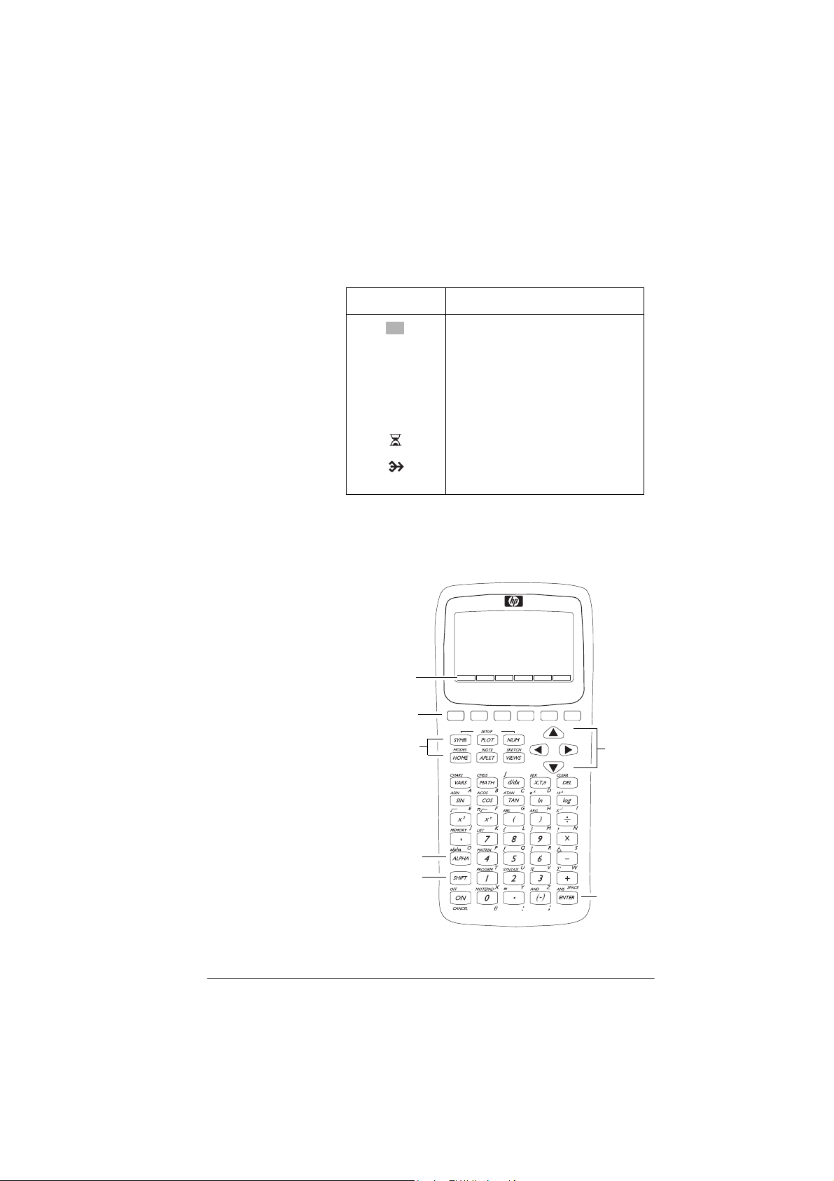
Title

History

Edit line

Menu key labels

Menu key or soft key labels. The labels for the menu keys’ current meanings. this picture. “Press

672?a

is the label for the first menu key in

672?a

” means to press the first menu key,

that is, the leftmost top-row key on the calculator keyboard.

Edit line. The line of current entry. History. The HOME display (>+20(@) shows up to four lines

of history: the most recent input and output. Older lines scroll off the top of the display but are retained in memory.

Title. The name of the c u rr e nt a pl et i s d is played at the top of the HOME view. RAD, GRD, DEG specify whether Radians, Grads or Degrees angle mode is set for HOME. The 'and ( symbolsindicate whether there is more history in the HOME display. Press the *e,and *k, to scroll in the HOME display.

NOTE

The HP 40G is packaged with a computerized algebra system

&$6_

(CAS). Press

to access the computerized algebra system. This User’s Guide contains images from the HP39G and do not display the

1-2 Getting started

&$6_

menu key label.

The keyboard

Menu keys

Annunciators. Annunciators are symbols that appear above the title bar and give you important status information.

Annunciator Description

Shift in effect for next keystroke. To cancel, press >6+,)7@ again.

α Alpha in effect for ne xt ke ys tr oke.

To cancel, press >$/3+$@ again.

((•)) Low battery power.

Busy.

Data is being transferred via infrared

or cable.

Menu key

labels

Menu keys

Aplet control

keys

Alpha key

Shift key

Getting started 1-3

Cursor

keys

Enter key

Aplet control keys

• On the calculator keyboard, the top row of keys are

called menu keys. Th eir meanings depend on the context—that’s why their tops are blank. The menu keys are sometimes called “soft keys”.

• The bottom line of the display shows the labels for the

menu keys’ current mea nings.

The aplet control keys are:

Key Meaning

>6<0%@ Displays the Symbolic view for the

current aplet. See “Symbolic view” on page 1-15.

>3/27@ Displays the Plot view for the current

aplet. See “Plot view” on page 1-15.

>180@ Displays the Numeric view for the

current aplet. See “Numeric view” on page 1-15.

>+20(@ Displays the HOME view. See

“HOME” on page 1-1.

>$3/(7@ Displays the Aplet Library menu. See

“Aplet library” on page 1-15.

>9,(:6@ Displays the VIEWS menu. See “Aplet

views” on page 1-15.

1-4 Getting started

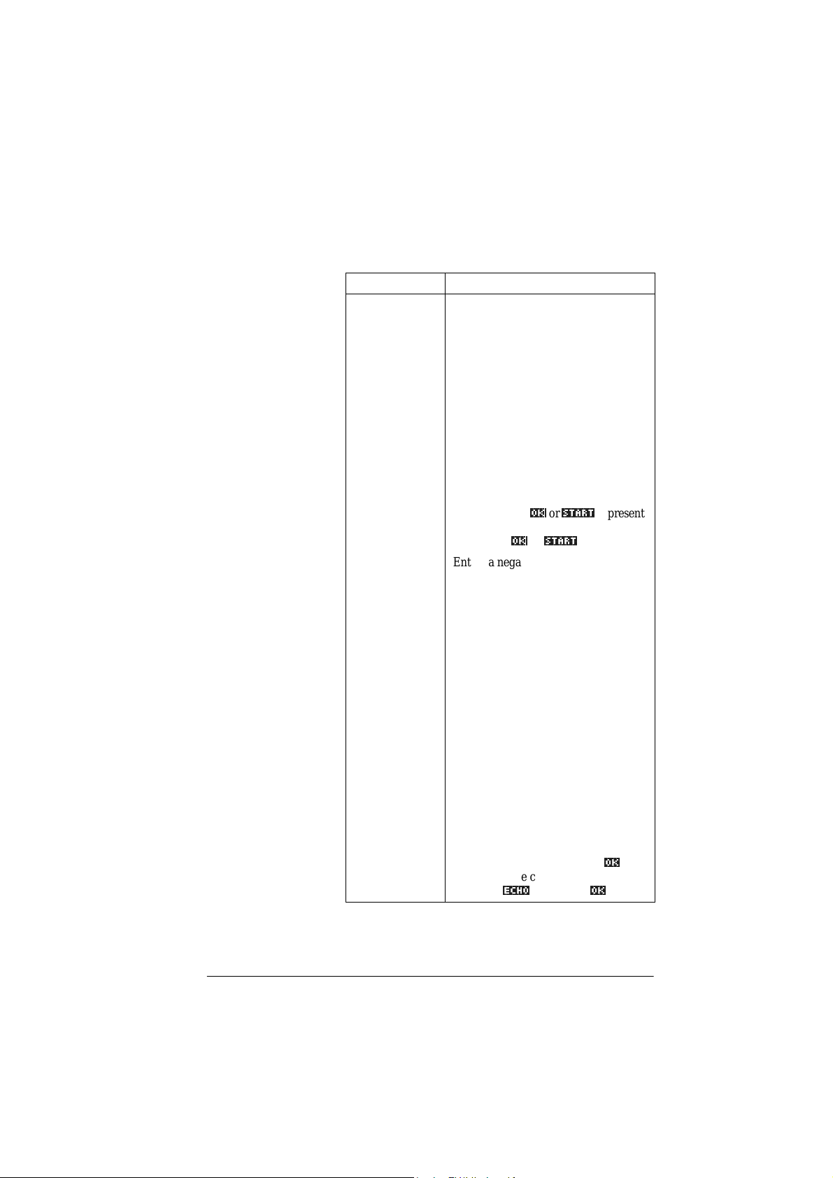
Entry/Edit keys The entry and edit keys are:

Key Meaning

>21@ (CANCEL) Cancels the current operation if t he

calculator is on by pressing >21@. Pressing >6+,)7@, then calculator off.

>6+,)7@ Accesses the function printed in blue

above a key.

>+20(@ Returns to the HOME view, for

>$/3+$@ Accesses the alphabetical characters

>(17(5@ Enters an input or execu tes an

>@ Enters a negative number. To enter

>;75@ Enters the independent variable by

>'(/@ Deletes the character under the cursor.

CLEAR Clears all data on the screen. On a

>6+,)7@

*>,, *A,, *k,, *e,

CHARS Displays a menu of all available

>6+,)7@

performing calculations .

printed in orange below a key. Hold down to enter a string of characters.

operation. In calculations, >(17(5@ acts

like “=”. When as a menu key, >(17(5@ acts the same as pressing

–25, press >@25. Note: this is not the

same operation tha t the su btract button performs (

inserting X, T, θ, or N into the e dit line, depending on the current active aplet.

Acts as a backspace key if the cursor is at the end of the line.

settings screen, for example Plot Setup, >6+,)7@ to their default values.

Moves the cursor around the display. Press beginning, end , top or bottom.

characters. To type one, use the arrow keys to highlight it, and press select multiple characters, select each and press

OFF turns the

2.a

67$57a

is present

2.a

67$57a

>@).

CLEAR returns all settings

>6+,)7@ first to move to the

2.a

(&+2a

, then press

2.a

. To

Getting started 1-5

Shifted keystrokes

There are two shift keys that you use to access the operations and characters printed above the keys:>6+,)7@ and >$/3+$@.

Key Description

>6+,)7@ Press the >6+,)7@ key to access the

operations printed in blue above the keys. For instance, to access the Modes screen, press >6+,)7@, then press >+20(@.

MODES is labelled in blue above the

( >+20(@ key). You do not need to hold down >6+,)7@ when you press HOME. This action is d epicte d in this m anua l as

“press >6+,)7@

MODES.”

To cancel a shift, press >6+,)7@ again.

>$/3+$@ The alphabetic keys are also shi fted

keystrokes. For instance, to type Z, press >$/3+$@Z. (The letters are printed in orange to the lower right of each key. )

To cancel Alpha, press >$/3+$@ again. For a lower case letter, press

>6+,)7@>$/3+$@. For a string of letters, hold down

>$/3+$@ while typing.

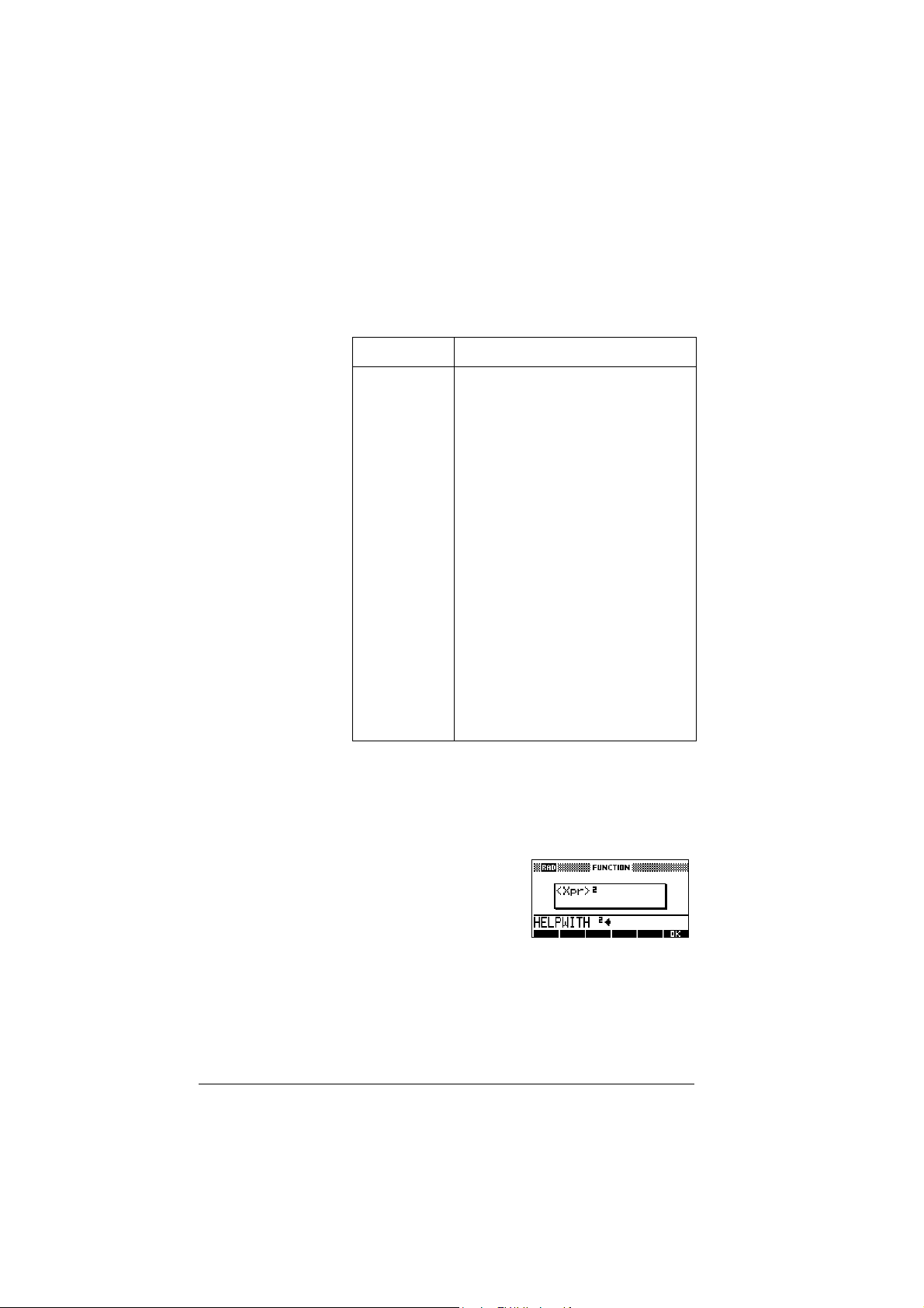
HELPWITH The HP 39G built-in help is available in HOME only. It

provides syntax help for built-in math fun ction s . Access the HELPWITH command by pressing >6+,)7@

and then the math key for which yo u require syntax help.

Example Press>6+,)7@

SYNTAX

>[@ >(17(5@

Note: Remove the left parenthesis from built-in commands such as sine, cosine, and tangent before invoking the HELPWITH command.

1-6 Getting started

SYNTAX

Math keys HOME (>+20(@) is the place to do calculations.

Keyboard keys. The most common operations are available from the keyboard, such as the arithmetic (like >@) and trigonometric (like >6,1@) functions. Press >(17(5@ to complete the operation: >6+,)7@√ 256>(17(5@ displays 16.

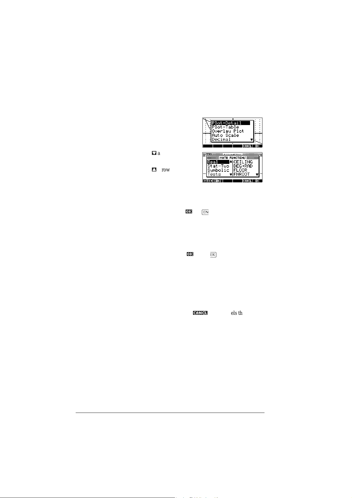
MATH menu. Press >0$7+@ to open the MATH menu. The MATH menu is a comprehensive list of math functions that do not appear on the keyboard. It also incl udes categories for all other functions and constants. The functions are grouped by category, ranging in alphabetical order from Calculus to Trigon ometry.

– The arrow keys scroll through the list (*e,, *k,) and

move from the category list in the left column to the item list in the right column(*>,, *A,).

2.a

to insert the selected com mand on to the ed it

&$1&/a

to dismiss the MATH menu without

&216a

displays the list of Program

07+a

takes you to the beginning of the

HINT

– Press

line.

– Press

selecting a command.

– Pressing

Constants. You can use these in programs that you develop.

– Pressing

MATH menu.

See “Math functions by category” on page 10-3 for details of the math functions.

When using the MATH menu, or any menu on the HP 39G/ 40G , pressing an alpha key takes you straight to the first menu option beginnin g with that alpha chara cte r. With this method, you do not ne e d to press >$/3+$@ first. Just press the key that corresponds to the comma nd’s beginning alpha character.

Program commands

Pressing >6+,)7@CMDS d isplays the list of Program Commands. See “Programming commands” on page 15-14.

Inactive keys If you press a key that does not operate in the current context,

a warning symbol like this appears. There is no beep.

Getting started 1-7

Menus

A menu offers you a choice of items. Menus are displayed in one or two columns.

_

•The

To search a menu • Press *e, or *k, to scroll through the list. If you press

• If there are two columns, the left column shows general

• To speed-search a list (with no edit line), type the first

arrow in the display

means more items below.

A_

arrow in the display

means more items above.

>6+,)7@*e, or >6+,)7@*k,, you’ll go all the way to the end or the beginning of the list. Highlight the item you want

2.a

to select, then press

(or >(17(5@).

categories and the right colu mn shows specific contents within a category . Highlight a general category in the left column, then highlight an item in the right column. The list in the right column changes when a different category is highlighted. Press

2.a

or >(17(5@when you have

highlighted your selection.

letter of the word. For example, to find the Matrix category in >0$7+@, press >@, the Alpha“M”key.

• To go up a page, you can press >6+,)7@*>,. To go down a

page, press >6+,)7@*A,.

To cancel a menu Press >21@ (for CANCEL) or

&$1&/a

. This cancels the current

operation.

1-8 Getting started

Input forms

An input form shows several fields of information for you to examine and specify. After highlighting the fie ld to edit, you can enter or edit a number (or expression). You can also select

&+226a

options from a list ( to check (

_&+.a

). See below for an example of an input form.

). Some input forms include items

Reset input form values

To reset a default field va lue in an input f orm, move the cursor to that fi eld and pr ess >'(/@. To re set all default field value s in the input form, press >6+,)7@

Mode settings

You use the Modes input form to set the modes for HOME.

HINT

Although the numeric setting in Modes affects only HOME, the angle setting controls HOME and the current aplet. The angle setting selected in Modes is the angle setting used in both HOME and current aplet. To further con f igure an aplet, you use the SETUP keys (>6+,)7@>3/27@ and >6+,)7@>180@).

Press >6+,)7@MODES to access the HOME MODES input form.

Setting Options

Angle Measure

Angle values are:

Degrees. 360 degrees in a circle. Radians. 2π radians in a circle. Grads. 400 grads in a circle.

The angle mode you set is the angle setting us ed in both HOME a n d the current aplet. This is done to ensure that trigonometric calculations done in the current aplet and HOME gi ve the same result.

CLEAR.

Getting started 1-9

Setting Options (Continued)

Number Format

Decimal Mark

The number format mode you set is the number format used in both HOME and the current aplet.

Standard. Full-precision display. Fixed. Displays results rounded to a

number of decimal places. Example:

123.456789 becomes 123.46 in Fixed 2 format.

Scientific. Displays results with an exponent, one digit to the left of the decimal point, and the specifi ed number of decimal places. Example: 123.456789 becomes 1.23E2 in Scientific 2 fo rmat.

Engineering. Displays result with an exponent that is a multiple of 3, and the specified number of significant digits beyond the first one. Example: 123.456E7 becomes 1.23E9 in Engineering 2 format.

Fraction. Displays results as fractions based on the specified number of decimal places. Examples: 123.456789 becomes 123 in Fraction 2 format, and .333 becomes 1/3 and 0.142857 becomes 1/7.

See “Using fraction s” on page 1-24. Dot or Comma. Displays a number as

12456.98 (Dot mode) or as 12456,98 (Comma mode). Dot mode uses commas to separate elements in list s and mat rices, and to separate function arguments. Comma mode uses periods (dot) as separators in these contexts.

1-10 Getting started

Setting a mode

HINT

This example demonstrates how to change the angle measure from the default mode, radians, to degrees for the current aplet. The procedure is the same for changing number format and decimal mark modes.

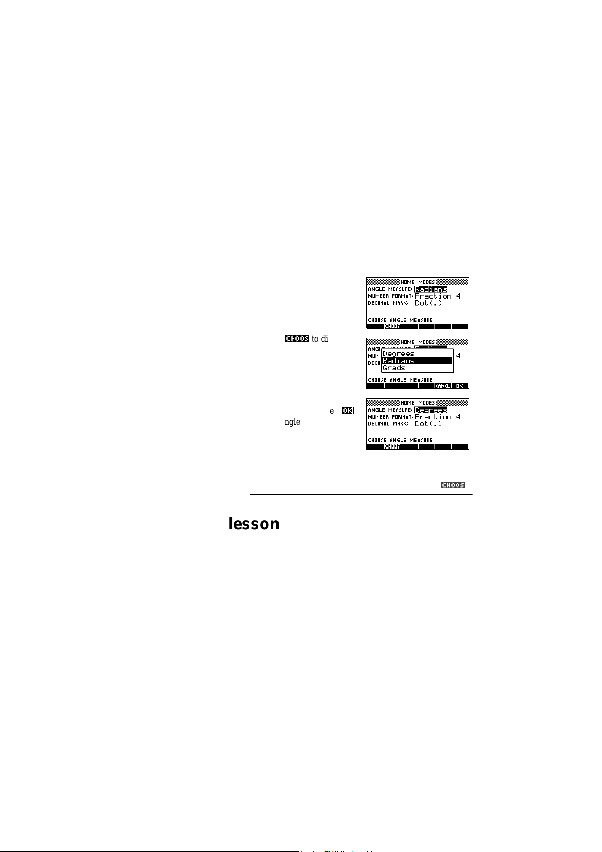
1. Press >6+,)7@MODES to open the HOME MODES input form.

The cursor (highlight) is in the first field, Angle Measure.

&+226a

2. Press

to display a

list of choices.

3. Press*k,to select Degrees,



and press

2.a

. The angle mea s ur e changes to degrees.

4. Press>+20(@ to return to HOME.

Whenever an input form has a list of choices for a field, you can press >@ to cycle through them instead of using

&+226a

Aplets (E–lessons)

Aplets are the application environments where you explore different classes of mathematical operations. You select the aplet that you want to work with.

Aplets come from a va ri e ty of so urces:

• Built-in the HP 39G/40G (initial purchase).

• Aplets created by saving existing aplets, which have been modified, with specific configurations. See “Creating new aplets based on existing aplets” on page 16-1.

• Downloaded from HP’s Calculators web site.

• Copied from another calculator.

Getting started 1-11

Aplets are stored in the Aplet

library. See “Aplet library” on page 1-15 for further information.

You can modify configuration settings for the graphical, tabular, and symbolic views of the aplets in the following table. See “Aplet view configuratio n ” on page 1-17 for further information.

Aplet

Use this aplet to explore:

name

Function Real-valued, rectangular functions y in

terms of x. Example: .

y 2x23x 5++=

Inference Confidence intervals and Hypothesis tests

based on the Normal and Students-t distributions.

Parametric Parametric relations x and y in terms of t.

Example: x = cos(t) an d y = sin(t).

Polar Polar functions r in terms of an angle θ.

Example: .

r 24θ()cos=

Sequence Sequence functions U in terms of n, or in

terms of previous terms in the same or another sequence, such as and

. Example: , and

n 2–

U10= U21=

n 1–

Solve Equations in one or more real-valued

variables. Example: .

x 1+ x

n 1–

x–2–=

Statistics One-var iable (x) or two-var iable (x and y)

statistical data.

In addition to these aplets, which can be used in a variety of applications, the HP 39G/40 G is supplied with two teaching aplets: Quad Explorer and Trig Explorer. You cannot modify configuration settings for these aplets.

A great many more teaching aplets can be found at HP’s web site and other web sites created by educa tors, together with accompanying documentation, often with student work sheets. These can be downloaded free of charge and transferred to the HP 39G/40G using the separately supplied Connectivity Kit.

1-12 Getting started

Quad Explorer aplet

The Qu ad Explo rer aplet is used to inve stigate the behaviour of as the values of a, h and v change, bo th

yaxh+()

v+= by manipulating the equation and seeing the change in the graph, and by manipulating the graph and seeing the change in the equation.

HINT

More detailed documentation, and an accompanying student

work sheet can be found at HP’s web site.

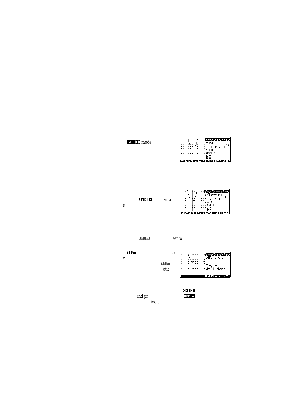
When first started, the aplet is

*53+aa

mode, in which the arrow keys, the >@ and >@ keys and the>@ key are used to change the shape of the graph. This changing shape is reflected in t he equation displayed at the top right corner of the screen, while the original graph is retained for comparison. In this mode th e graph controls the equation.

It is also possibl e to have the equation control the gra ph. Pressing

6<0%a

displays a

sub-expression of your equation (see right).

Pressing the *A,and *>,key moves between subexpressions, while pressing the *k,and*e, key changes their values.

/(9(/a

Pressing

allows the user to select wheth er all three sub-

expressions will be explored at once or only one at a time. A

7(67a

button is provided to

evaluate the student’s knowledge. Pressing

7(67a

displays a target quadratic graph. The student must manipulate the equation’s parameters to make the equation match the target graph. Wh en a student feels that they have

&+(&.a

correctly chosen the parameters a answer and provide feedback. An

button evaluates t he

$16:a

button is provided

for those who give up!

Getting started 1-13

Trig Explorer aplet

The Trig Explorer aplet is used to investigate the behaviour of the graph of as the values of a, b, c

ya bxc+()d+sin=

and d change, both by manipulating the equation and seeing the change in the graph, or by manipulating the graph and seeing the change in the equa tion.

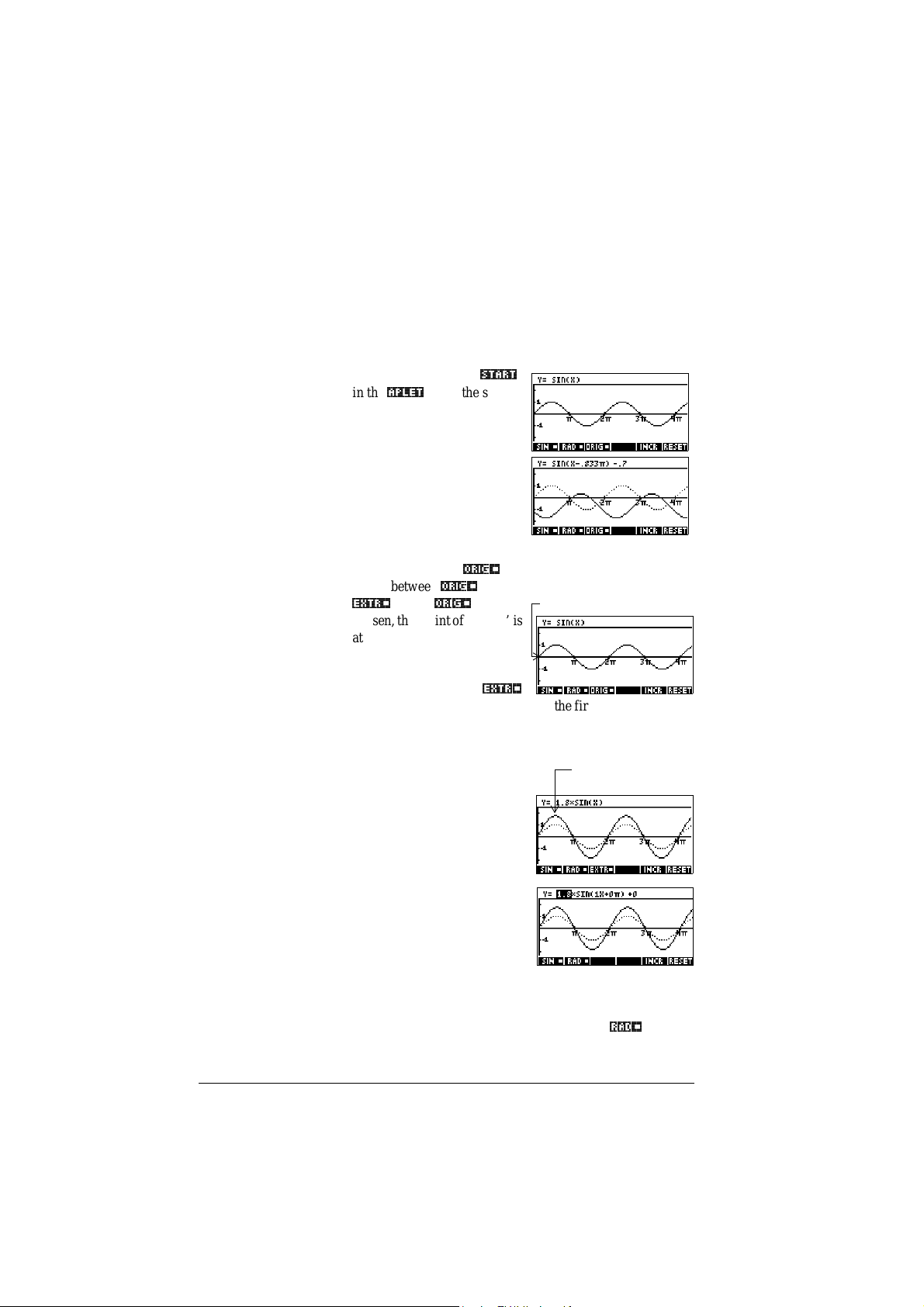
67$57a

When the user presses

$3/(7a

in the

view, the screen

shown right is displ a yed.

In this mode, the graph controls the equation. Pressing the *k,*e, and *>,*A, keys transforms the graph, with these transformations reflected in the equation.

25,*aa

and

is a

Origin

The button labelled toggle between

(;75aa

. When

25,*aa

chosen, the ‘point of control’ is at the origin (0,0) and the *k,*e, and *>,*A, keys control vertical and horizontal

(;75aa

transformations. When is chosen the ‘point of control’ is on the first extremum of the graph (i.e. for the sine gr aph at .

π 21,⁄()

The arrow keys change the amplitude and frequency of the

Extremum

graph. This is most easily seen by experimenting.

Pressing >6<0%@ displays the equation at the top of the screen. The equation is controls the graph. Pressing the *A, and *>, keys move s from parameter to parameter. Pressing the *k, or *e, key changes the parameter’s va lue s .

The default angle setting for this aplet is radians. The angle

5$'aa

setting can be changed to degrees by pressing

1-14 Getting started

Aplet library

Aplets are stored in the Aplet library.

To open an aplet Press >$3/(7@ to display the Aplet library menu. Select the

aplet and press From within an aplet, you can return to HOME any time by

pressing >+20(@.

67$57_

or >(17(5@.

Aplet views

When you have configured an aplet to define the relation or data that you want t o explore, you can display i t in different views. Here are illustrations of the three major apl et vi ews (Symbolic, Plot, an d Numeric), th e six supporting aplet views (from the VIEWS menu), and the two user-defined views (Note and Sketch).

Symbolic view Press >6<0%@ to display the aplet’s Symbolic view.

Y o u use this view to define the function(s) or equation(s) that you want to explor e.

See “About the Symbolic view” on page 2-1 for further information.

Plot view Press >3/27@ to display the aplet’s Plot view.

In this view, the functions that you have defined are displayed graphically .

See “About the Plot view ” on page 2-5 for further information.

Numeric view Press >180@to display the aplet’s Numeric view.

In this view, the functions that you have defined are displayed in tabular format.

See “About the numeric view” on page 2-15 for further information.

Getting started 1-15

Plot-Table view

The VIEWS menu contains the Plot-Table view. >9,(:6@

Select Plot-Table Splits the screen into the plot

and the data table. See “Other

views for scaling and splitting the graph” on page 2-13 for futher information.

2.a

Plot-Detail view

Overlay Plot view

The VIEWS menu contains the Plo t-Detail view. >9,(:6@

Select Plot-Detail Splits the screen into the plot

and a close-up. See “Other views for scaling and splitting the graph” on

page 2-13 for further information.

The VIEWS menu contains the Overlay Plot view.

>9,(:6@

Select Overlay Plot Plots the current expression(s)

without erasing an y pre existing plot(s) .

See “Other views for scaling and splitting the graph” on page 2-13 for further information.

2.a

Note view Press >6+,)7@NOTE to display the aplet’s note view.

This note is transferred with the aplet if it is sent to another calculator or to a PC. A note view contains text to supplement an aplet.

See “Notes and sketches” on page 14-1 for furthe r information.

Sketch view Press >6+,)7@SKETCH to display the aplet’s sketch view.

1-16 Getting started

Displays pictures to supplement an aplet.

See “Notes and sketches” on page 14-1 for further information.

Aplet view configuration

You use the SETUP keys (>6+,)7@>3/27@,and >6+,)7@>180@) to configure the aplet. For example, pr ess >6+,)7@ (>6+,)7@>3/27@)to display the input form for setting the aple t’s plot settings. Angle measure is controlled using the view.

Plot Setup Press>6+,)7@SETUP-PLOT. Sets

parameters to plot a graph.

Numeric Setup Press >6+,)7@SETUP-NUM. Sets

parameters for building a table of numeric valu es .

SETUP-PLOT

MODES

Symbolic Setup

This view is only available in the Statistics aplet in 2VAR mode, where it plays an important role in choosing data models. Press (>6+,)7@

SYMB.

SETUP

To change views Each view is a separate environment. To change a view, select

a different view by pressing >6<0%@, >180@, >3/27@ keys or select a view from the VIEWS menu. To change to HOME, press >+20(@. You do not explicitly close the current view, you just enter anot her one—like passing from one room into another in a house. Data that you enter is automati cally sav ed as you enter it.

To save aplet configuration

Getting started 1-17

You can save an aplet configuration that you have used, and transfer the aplet to other HP 39G/40G calculators. See “Sending and receiving aplets” on page 16-5.

Mathematical calculations

The most commonly used math operations are available from the keyboard. Access to the rest of the math functions is via the MATH menu (>0$7+@).

To access programming command s, press >6+,)7@

“Programming commands” on page 15-14 for further information.

CMDS. See

Where to start The home base for the calculator is the HOME view

(>+20(@). You can do all calculations here, and you can access all >0$7+@ operations.

Entering expressions

Example Calculate :

• Enter an expression into the HP 39G/40G in the same left-to-right order that you would write th e expression. This is called algebraic entry.

• To enter functions, select the key or MATH menu item for that function. You can also enter a function by using the Alpha keys to spell o ut its name.

• Press >(17(5@ to evaluate the expression you have in the edit line (where the blinking cursor is). An expression can contain numbers, functi ons, and variables.

14 8–

----------------------------

>@23>[, >@14 >;@>6+,)7@√ 8>@ >j@>@3 >OQ@45 >@ >(17(5@

3–

45()ln

Long results If the result is too long to fit on the display line , or if you want

to see an expression in textbook format, press *k, to highlight

6+2:a

it and then press

Negative numbers

1-18 Getting started

Type >@to start a negative numb er or to insert a nega tiv e sign.

To raise a negative number to a power, enclose it in parentheses. For example, (–5)

= 25, whereas –52 = –25.

Scientific notation (powers of 10)

A number like or is written in scientific notation, that is, in terms of powers of ten. This is simpler to

work with than 5000 0 or 0.0000 00321. To e nter numbe rs like these, use

Example Calculate

>@4 >6+,)7@EEX >@13>@ >;@>@6 >6+,)7@

23>@ >j@ 3 >6+,)7@EEX >@5

>(17(5@

510

× 3.21 107–×

EEX. (This is easier than using >;@10>[N@.)

13–

410

×()610

---------------------------------------------------310

EEX

×()

5–

Explicit and implicit multiplication

HINT

Implied multiplication takes place when two operands appear with no operator in between. If you enter AB, for example, the result is A*B.

However, for clarity, it is better to include the multiplication sign where you expect multiplication in an expression. It is clearest to enter AB as A*B.

Implied multiplication will not alway s work as expect ed. For example, entering A(B+4) will not give A*(B+4). Instead

an error message is displ ayed: “Invalid User Function”. T his is because the calculator interprets A(B+4) as meaning ‘evaluate function A at the va l u e B+4’, and function A does not exist. When in doubt, insert the * sign manually.

Getting started 1-19

Parentheses You need to use parentheses to enclose arguments for

functions, such as SIN(45). You can omit the final parenthesis at the end of an edit line. The calculator inserts it automatically.

Parentheses are also important in specifying the order of operation. Without parentheses, the HP 39G/40G calculates according to the order of algebraic precedence (the next topic). Following are some examples using parentheses.

Entering... Calculates...

>6,1@ 45>@ >6+,)7@π sin (45 + π) >6,1@45>@ >@>6+,)7@π sin (45) + π

Algebraic precedence order of evaluation

Largest and smallest numbers

>6+,)7@√85>;@ 9 >6+,)7@√>@ 85>;@9>@

Functions within an expression are evalu ated in the following order of precedence. Functions with the same precedence are evaluated in order from left to right.

1. Expressions within parentheses. Nested parentheses are evaluated from inner to outer.

2. Prefix functions, such as SIN and LOG.

3. Postfix functions, such as !

4. Power function, ^, NTHROOT.

5. Negation, multi plication, and division.

6. Addition and subtraction.

7. AND and NOT.

8. OR and XOR.

9. Left argument of | (where).

10. E quals, =.

The smallest number the HP 39G/40G can represent is

–499

1×10 largest number is 9.99999999999 × 10

still displayed as this number.

(1E–499). A sma ller result is displa yed as zero. The

85 9× 85 9×

–49

. A larger result is

1-20 Getting started

Clearing numbers

• >'(/@ clears the character under the cursor. When the cursor is positioned after the last character, >'(/@ deletes the character to the left of the cursor, that is, it performs the same as a backspace key.

•

CANCEL (>21@) clears the edit line.

Using previous results

To copy a previous line

To reuse the last result

• >6+,)7@

CLEAR clears all input and output in the display,

including the display history.

The HOME display (>+20(@) shows you four lines of input/ output history. An unlimited (except by memory) number of previous lines can be displayed by scrolling. You can retrieve and reuse any of these values or expr essions.

Input

Last input

Edit line

Output

Last output

When you highligh t a previous input or result (by pressing

&23<a

and

6+2:a

*k,), the

Highlight the line (press *k,) and press

menu labels appear.

&23<a

. The number (or

expression) is copied into th e edit line.

Press >6+,)7@ANS (last answer) to put the last result from the HOME display into an expression.

ANS is a variable that is

updated each time you press >(17(5@.

To repeat a previous line

To repeat the very last line, just press >(17(5@. Otherwise, highlight the line (pre ss *k,) first, and then press >(17(5@. The highlighted expression or number is re-entered. If the previous line is an expression containing the

ANS, the

calculation is repeated iteratively.

Getting started 1-21

Example See how >6+,)7@ANS retrieves and reuses the last result (50),

and >(17(5@ updates

ANS (from 50 to 75 to 100).

50>(17(5@ >@25 >(17(5@>(17(5@

You can use the last result as the first expressio n i n the edit line without pressing >6+,)7@

ANS. Pressing >@, >@, >;@, or

>j@, (or other operators that require a preceding argument)

automatically enters ANS before the operator. You can reuse any othe r expression or value in the HOME

display by highlighting the expression (using the arrow keys), then pressing

&23<a

. See “Using previ ous results” on page 1-

21 for more details. The variable

display history. A value in

ANS is different from the numbers in HOME’s

ANS is stored internally with the fu ll

precision of the ca lculated result, whereas the displayed numbers match the dis p la y mo de .

HINT

When you retrieve a num b er fr om ANS , you obtain the result to its full precision. When you retrieve a number from the HOME’s display histor y, you obtain exactly what was displayed.

Pressing >(17(5@ evaluates (or re-evaluates) the last input, whereas pressing >6+,)7@

ANS copies the last result (as ANS) into

the edit line.

1-22 Getting started

Storing a value in a variable

You can save an answer in a variable and use the variable in later calculations. There are 27 variables available for storing real values. These are A to Z and θ. See Chapter 11,

“Variables and memory management” for more inf ormation on variables. For example:

1. Perfor m a ca l c ulation. 45>@8 >[8@3

>(17(5@

2. Store the result in the A variable.

672a?a

>$/3+$@A >(17(5@

3. Perform anot he r cal c ula tio n usin g the A va r ia b le . 95>@2>;@ >$/3+$@A

Accessing the display history

Pressing *k, enables the highlight bar in the display history. While the highlight bar is active, the following menu and keyboard keys are very useful:

Key Function

*k,, *e, Scrolls through the display history.

&23<a

Copies the highlighted expression to the position of the cursor in the edit line.

6+2:a

Displays the current expression in standard mathematical form.

>'(/@ Deletes the highlighted expression from

the display h istor y, unle ss ther e is a cu rsor in the edit line.

>6+,)7@

CLEAR

Getting started 1-23

Clears all lines of display history and the edit line.

Clearing the display history

It’s a good habit to clear the display history (>6+,)7@CLEAR) whenever you have finished working in HOME. It saves calculator memory to clear the displa y history. Remember that all your previous inputs and results are saved unt il you clear them.

Using fractions

To work with fractions in HOME, you se t the num ber format to Fractions, as follows:

Setting Fraction mode

1. In HOME, open the HOME MODES input form.

MODES

>6+,)7@

2. Select Number Format and press options, then select Fraction.

&+226a

2.a

*A,

*e,*e,*e,*e,

to select the

*e,

3. Press option, then select the precision value.

2.a

4. Enter the precision that you want to use, and press set the precision. Press >+20(@ to return to HOME.

See “Setting fraction precision” below for more information.

&+226a

to display the

2.a

1-24 Getting started

Setting fraction precision

The fraction precision setting determines the precision in which the HP 39G/40G converts a decimal valu e to a fraction. The greater the precision value that is set, the closer the fraction is to the decimal value.

By choosing a precisi on of 1 you are saying that the fraction only has to match 0.234 to at least 1 decimal place (3/13 is

0.23076...). The fractions us ed are foun d using th e techniqu e of contin ued

fractions. When converting recurring decimals this can be important.

For example, at precis ion 6 the decimal 0.6666 becomes 3333/5000 (6666/10000) whereas at precision 3, 0.6666 becomes 2/3, which i s probably what you would want.

For example, when converting .234 to a fraction, the precision value has the following effect:

• Precision set to 1:

• Precision set to 2:

• Precision set to 3:

• Precision set to 4

Getting started 1-25

Fraction calculations

When entering fractions:

• You use the>j@ key to separate the numerator part and the denominator part of the fraction.

• To enter a mixed fraction, for example, 1

in the format (1+

For example, to perform the following calculation: 3(23/4 + 57/8)

1. Set the mode Number format to fraction. >6+,)7@MODES *e,

&+226a

Select

Fraction

>(17(5@*A,4

2. Return to HOME and enter the calculation. 3>;@>@>@2>@3

>j@4>@>@>@5>@7 >j@8>@>@

3. Evaluate the calculation.

>(17(5@

/2).

2.a

/2, you enter it

Converting decimals to fractions

1-26 Getting started

To convert a decimal value t o a fract ion:

1. Set the number mode to Fraction.

2. Either retrieve the value from the History, or enter the value on the command line.

3. Press >(17(5@ to convert the number to a fraction.

Converting a number to a fraction

When converting a number to a fraction, keep the following points in mind:

• When converting a recurring decimal to a fraction, set the fraction precision to about 6, and ensure that you include more than six decimal places in th e recurring decimal that you enter.

In this example, the fraction precision is set to 6. The top calculation returns the correct result. The bottom one does not.

• To con vert an ex act d e cimal to a fra ction , set th e fractio n precision to at least two more than the numb er of decimal places in the decimal.

In this example, the fraction precision is set to 6.

Complex numbers

Complex results The HP 39G/40G can return a complex number as a result for

some math functions. A complex number appears as an ordered pair (x, y), where x is the real part and y is the imaginary part. For example, entering returns (0,1).

1–

To enter complex numbers

Getting started 1-27

Enter the number in either of these forms, where x is the real part, y is the imaginary part, and i is the imagina ry consta nt,

1–

• (x, y) or

• x + iy.

To enter i:

• press >6+,)7@>$/3+$@I or

• press >0$7+@, *k,or *e,keys to select Constant, *A, to move to the right co lumn of the menu, *e,toselect i, and

2.a

Storing complex numbers

There are 10 variables available for storing complex numbers: Z0 to Z9. To store a complex number in a variable:

• Enter the comple x number, press

672a?a

,enter the

variable to store the number in and press >(17(5@.

>@4>@5>@ >$/3+$@Z 0 >(17(5@

Catalogs and editors

The HP 39G/40G has several catalo gs an d editors. You use them to create and manipulate objects. They access features and stored values (numbers or text or other items) that are independent of aplets.

•A catalog lists items, which you can delete or transmit, for example an aplet.

•An editor lets you create or modify item s and numbers, for example a note or a matr ix.

Catalog/Editor Contents

Aplet library (>$3/(7@)

Sketch editor

SKETCH)

(>6+,)7@ List (>6+,)7@

LIST) Lists. In HOME, lists are enclosed

672a?_

Aplets.

Sketches and diagrams, See Chapter 14, “Notes and sketches”.

in {}. See Chapter 13, “Lists”.

Matrix (>6+,)7@

MATRIX)

One- and two-dimens ional arrays. In HOME, arrays are enclosed in []. See Chapter 12, “Matrices”.

Notepad (>6+,)7@NOTEPAD)

Program

PROGRAM)

(>6+,)7@

Notes (short text entries). See Chapter 14, “Notes and sketches”.

Programs that you create, or associated with user-defined aplets. See Chapter 15, “Programming”.

1-28 Getting started

Differences between the HP 38G and the HP 39G/40G

CAS The HP 40G is packaged with a comput er algebra system

(CAS). Refer to the CAS Manual for further information.

Memory manager

Plot Goto function

Statistics Pred function

The HP 39G/40G incorp or ates a memory manager that you can use to see how much memory the objects that you have

created or loaded are occupying. See “Memory Manager” on page 11-9 for more information.

In Plot view, you can use the value on the plot instead of having to trace the plot to locate values. See “Expl oring the graph” on page 2-7 for more information.

When you choose the view screen, it is now possible to curve. Once a data set and regressi on curve is displayed, pressing the up an d down a rrow s wi ll move betwe en the data and the curve of regression. When th e regression curve is selected, the values displayed in the Plot view status line are the PREDY values. On the HP 38G, the Trace function would select known data points on ly.

*272a

menu key to jump to a

),7a

option in the Statistics aplet’s Plot

75$&(a

along the regression

Inference aplet To complement the St atistics aplet, a new Infe rence aple t has

been added. Use this aplet to perform hypothesis tests and determine confidence intervals. See “About the Inference aplet” on page 9-1 for more information.

Trig Explorer and Quadratic Explorer

The teaching aplets Trig Explorer and Quadratic Explorer have been added to the calculator. These two aplets add powerfully to the capabilities of the calculator in the classroom.

aplets

Getting started 1-29

Aplets and their views

Aplet views

This section examines the options and functionality of the three main views for the Function, Polar, Parametric, and Sequence aplets: Symbol ic, Plot, and Numeric views.

About the Symbolic view

The Symbolic view is the defining view for the Function, Parametric, Polar, and Sequence aplets. The other views are derived from the symbolic expression.

You can create up to 10 different definitions for each Function, Parametric, Polar, and Sequence aplet. You can graph any of the relations (in the same aplet) simultaneo usly by selecting them.

Defining an expression (Symbolic view)

Choose the aplet from the Aplet Libr ary.

>$3/(7@

Press *k,or*e, to select an aplet.

67$57_

The Function, Parametric, Polar, and Sequence aplets start in the Symbolic view.

If the highlight is on an existing expression, scroll to an

empty line—unless you don’t mind writing over the expression—or, clear one line (>'(/@) or all lines (>6+,)7@CLEAR).

Expressions are selected (check marked) on entry. To deselect an expression, press expressions are plotted.

Aplets and t heir views 2-1

_&+._

. Allselected

– For a Function

definition, enter an expression to define F(X). The only independent variable in the expression is

– For a Parametric

definition, enter a

pair of expressions to define X(T) and Y(T). The only independent variable in the expressions is T.

– For a Polar

definition, enter an expression to define R(θ). The only independent variable in the expression is

θ.

– For a Sequence

definition, either:

Enter the first and second terms for U (U1, or... U9, or U0). Define the nth term of the sequenc e in terms of N or of the prior terms, U(N–1) and U(N–2). The expressions

should produce real-valued sequences with integer domains.Or define the nth term as a non-recursive expression in terms of n only. In this case, the calculator inserts the first two terms based on the expression that you d e f ine.

2-2 Aplets and their views

Evaluating expressions

In aplets In the Symbolic view, a variable is a symbol only, and does

not represent one specific value. To evaluate a function in

(9$/_

Symbolic view, press function, then

(9$/_

in terms of their independent variab le.

1. Choose the Functio n aplet.

>$3/(7@

Select Function

67$57_

2. Enter the expressions in

the Function aplet’s Symbolic view.

>$/3+$@A >;@ >[@

__2.__

>$/3+$@B >$/3+$@F1 >@ >$/3+$@F2 >@ >@

__2.___

_;__

__2.___

_;__ _;__

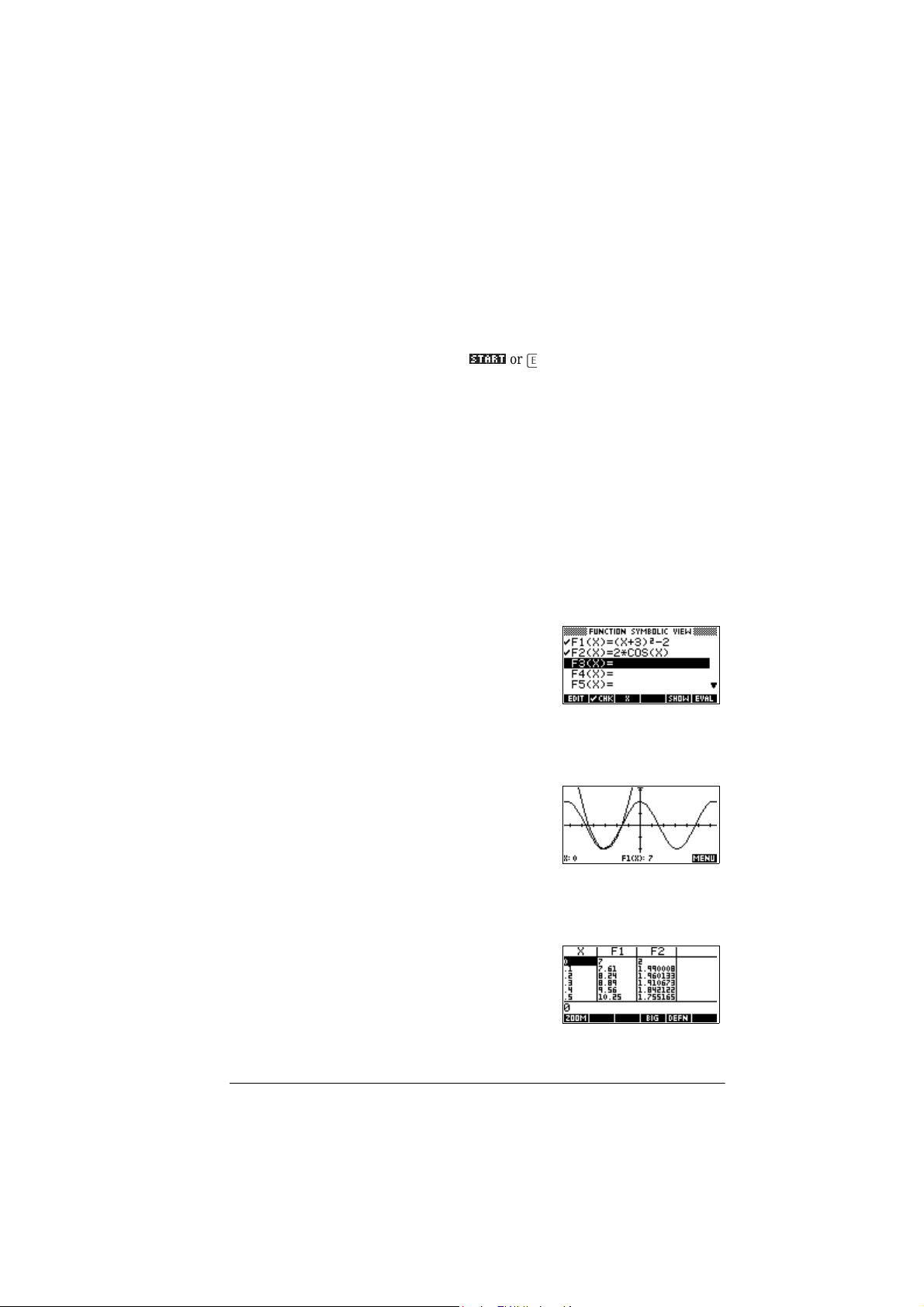
3. Highlight F3(X).

*k,

. If a function calls another

resolves all references to other functions

>@>@

4. Press

(9$/_

Note how the values for F1(X) and F2(X) are substituted into F3(X).

In HOME You can also evaluate any expression in HOME by entering it

into the edit line and pressing>(17(5@. For example, define F4 as below. In HOME, type F4(9)and

press >(17(5@. This evaluates the expression, sub stituting 9 in place of X into F4.

Aplets and t heir views 2-3

SYMB view keys

The following table details the menu keys that you use to work with the Symbolic view.

Key Meaning

(',7_

Copies the h ighlight ed expre ssion to th e

2._

edit line for editing. Press

when

done.

_&+._

Checks/unchecks the current expression (or set of expressions). Only checked expression(s) are evaluated in the Pl ot and Numeric views.

__;___

Enters the independent variable in the Function aplet. Or, you can use the >;75@ key on the keyboard.

__7___

Enters the independent variable in the Parametric aplet. Or, you can use the >;75@ key on the keyboard.

_____

Enters the independent variable in the Polar aplet. Or, you can use the >;75@ key on the keyboard.

__1___

Enters the independent variable in the Sequence aplet. Or, you can use the >;75@ key on the keyboard.

6+2:_

Displays the current expression i n t ext book form.

(9$/_

Resolves all references to other definitions in terms of variables and evaluates all arithmetric expressions.

>9$56@ Displays a menu for entering variable

names or contents of variables.

>0$7+@ Displays the menu for entering math

operations.

>6+,)7@

CHARS

Displays special characters. To enter one, place the cursor on it and press

__2.___

. To remain in the CHARS menu and enter another special character, press

(&+2_

>'(/@ Deletes the highlighte d ex pression or

the current character in the edit line.

CLEAR Deletes all expressions in the list or

>6+,)7@

clears the edit line.

2-4 Aplets and their views

About the Plot view

After entering and selecting (check marking) the exp ression in the Symbolic view, press >3/27@. To adjust the appearance of the graph or the interv al tha t is displaye d, yo u can chang e the Plot view settings.

You can plot up to ten expressions at the same time. Select the expressions you want to be plotted together.

Setting up the plot (Plot view setup)

Press >6+,)7@SETUP-PLOT to define any of the settings shown in the next two tables.

1. Highlight the field to edit.

– If there is a number to enter, type it in and press

>(17(5@ or

– If there is an option to choose, press

your choice, an d pre s s>(17(5@ or

&+226_

to >@ to cycle through the options.

– If there is an option to select or deselect, press

to check or unchec k it.

2. Press

3$*(_

3. When done, press >3/27@ to view the new plot.

2._

, just highlight the field to change and press

to view more settings.

&+226_

, highlight

2._

. As a shortcut

_&+._

Plot view

The plot view settings are:

settings

Field Meaning

XRNG, YRNG Specifies the minimum and

maximum horizontal (X) and vertical (Y) values for the plotting window.

RES For function plots: Resolution;

“Faster” plots in alternate pixel columns; “Detail” plots in every pixel column.

TRNG Parametric aplet: Specifies the t-

values (T) for the graph.

θRNG Polar aplet: Specifies the angle (θ)

value range for the graph.

Aplets and t heir views 2-5

Field Meaning (Continued)

NRNG Sequence aplet: Specifies the index

(N) values for the graph.

TSTEP For Parametric plots: the increment

for the independent variable.

θSTEP For Polar plots: the increment value

for the independent variable.

SEQPLOT For Sequence aplet: Stairstep

or Cobweb types.

XTICK Horizontal spacing for tickmarks. YTICK Vertical spacing for tickmarks.

Those items with space for a checkmark are settings you can

3$*(_

turn on or off. Press

to display the second page .

Field Meaning

SIMULT If more than one relation i s being

plotted, plots them simultaneously (otherwise sequentially).

INV. CROSS Cursor crosshairs invert the status of

the pixels they cover.

CONNECT Connect the plotted points. (The

Sequence aplet always connects them.)

LABELS Label the axes with XRNG and YRNG

values.

AXES Draw the ax es. GRID Draw grid points using XTICK and

YTICK spacing.

Reset plot settings

To reset the default values for all plot settings, press

>6+,)7@

CLEAR in the Plot Setu p view. To reset the default valu e

for a field, highlight the field, and press >'(/@.

2-6 Aplets and their views

Exploring the graph

Plot view gives you a selection of keys and menu keys to explore a graph further. The options vary from aplet to aplet.

PLOT view keys

The following table details the k eys that y ou use to work with the graph.

Key Meaning

CLEAR Erases the plot and axes.

>6+,)7@ >9,(:6@ Offers additional pre-defined views for

splitting the screen and for scaling

(“zooming”) the ax es .

>6+,)7@*>,

Moves cursor to far left or far right.

>6+,)7@*A,

*k,

Moves cursor between relations.

*e,

3$86(_

or >21@ Interrupts plotting.

&217_

0(18_

Continues plotting if interrupted. Turns menu-key labels on and off. When

0(18_

the labels are off, pressing

turns

them back on.

0(18_

• Pressing

once displays the

full row of labels.

• Pressing

0(18_

a second time removes the row of labels to display only the graph.

• Pressing

0(18_

a third time displays the coordinate mode.

=220_

75$&(_

*272_

Displays ZOOM menu list. Turns trace mode on/off. A white box

appears over the

75$&(_

Opens an input form for you to enter an X (or T or N or θ) value. Enter the value and press

2._

. The cursor jumps to the point

on the graph that you en te re d.

)&1_

Function aplet only: Turns on menu list for root-finding functions (see “Analyse graph with FCN func tions” on page 3-3.

'()1_

Displays the current, defining expression. Press

0(18_

to restore the

menu.

Aplets and t heir views 2-7

Trace a graph You can trace along a function using the *>, or* A , key which

moves the cursor along the graph. The display also shows the current coordinate position (x, y) of the cursor. Trace mode and the coordin ate display ar e automatica lly set when a plot is drawn.

Note: Tracing might not appear to exactly follow your plot if the resolution (in Plot Setup view) is set to Faster. This is because RES: FASTER plots in only every other column, whereas tracing always uses every column.

In Function and Sequence Aplets: You can also scroll (move the cursor) left or right beyond the edge of the display window in trace mode, giving you a view of more of the plot.

To move between relations

To jump directly to a value

If there is more than one relation displayed, press *k, or *e, to move between relations.

To jump straight to a value rather than using the Trace function, use the value. Press

To turn trace on/ off

If the menu labels are not displayed, press

• Turn off trace mode by pressing

• Turn on trace mode by pressing

• To turn the coordinate display off, press

Zoom within a graph

One of the menu key opti ons is plot on a larger or smaller scale. It is a shor tc ut for changing the Plot Setup.

With the Set Factors option you can spec ify the factors tha t determine the extent of zoom in g, and whether the zoom is centered about the cursor.

ZOOM options Press

displayed, press all aplets.

Option Meaning

Center Re-centers the plot around the current

*272_

menu key. Press

2._

to jump to the value.

=220_

, select an option, and press

0(18_

.) Not all

position of the c ursor without changing the scale.

*272_

, then enter a

0(18_

75$&_

75$&(_

0(18_

=220_

. Zooming redraws the

2._

. (If

=220_

options are available in

first.

=220_

is not

Box... Lets you draw a box to zoom in on. See

“Other views for scaling and splitting the graph” on page 2-13.

2-8 Aplets and their views

Option Meaning (Continued)

In Divides horizontal and v ert ical scales

by the X-factor and Y-factor. For instance, if zoom factors are 4, then zooming in results in 1/4 as many units depicted per pixel. (see Set Factors)

Out Multiplies horizontal and vertical

scales by the X-factor and Y-factor (see Set Factors).

X-Zoom In Divides horizontal scale only, using

X–factor.

X-Zoom Out Multiplies horizontal scale, using

X–factor.

Y-Zoom In Divides vertical scale only, using

Y–factor.

Y-Zoom Out Multiplies vertical scale only, using

Y–factor.

Square Changes the vertical scale to match the

horizontal scale. (Use this after doing a Box Zoom, X–Zo om, or Y–Zoom.)

Set Factors...

Sets the X–Zoom and Y–Zoom factors for zooming. Includes option to recenter the plot before zooming.

Auto Scale Rescales the vertical axis so that th e

display shows a representative piece of the plot, for the supplied x axis settings. (For Sequence and Statistics aplets, autoscaling rescales both axes.)

The autoscale process uses the first selected function only to determine the best scale to use.

Decimal Rescales both axes so each pixel = 0.1

units. Resets default values for XRNG (–6.5 to 6.5) and YRNG (–3.1 to 3.2). (Not in Sequence or Statistics aplets. )

Aplets and t heir views 2-9

Option Meaning (Continued)

3 xsin

Integer Rescales horizontal axis only, making

each pixel =1 unit. (Not available in Sequence or Statistics aplets.)

Trig Rescales horizontal axis so

1 pixel = π/24 radian, 7.58, or

/3grads; rescales vertical axis so

8 1 pixel = 0.1 unit. (Not in Sequence or Statistics aplets.)

Un-zoom Returns the display to the previous

zoom, or if there has been only one zoom, un-zoom displays the graph with the original plot settings.

ZOOM examples The following screens show the effects of zooming options on

a plot of . Plot of

Zoom In:

0(18_ =220_

2._

Un-zoom:

=220_

Un-zoom

2._

(Press *k, to move to the bottom of the Zoom list.)

Zoom Out:

=220_

Out

2._

Now un-zoom.

2-10 Aplets and their views

X-Zoom In:

=220_

X-Zoom In

Now un-zoom.

X-Zoom Out:

=220_

X-Zoom Out

Now un-zoom.

Y-Zoom In:

=220_

Y-Zoom In

Now un-zoom.

Y-Zoom Out:

=220_

Y-Zoom Out

Zoom Square:

2._

=220_

Square

Aplets and t heir views 2-11

2._

To box zoom The Box Zoom option lets you draw a box around the area you

want to zoom in on by sele cting the e ndpoints of one dia gonal of the zoom rectangle.

0(18_

1. If necessary, press

2. Press

=220_

and select

3. Position the cursor on one corner of the rectangle. Press

2._

4. Use the cu rs or ke ys (*e,, etc.) to drag to the opposite corner.

2._

5. Press

to zoom in on

the boxed area.

to turn on the menu-key labels.

%2;_

To set zoom factors

1. In the Plot view, press

=220_

2. Press

0(18_

3. Select Set Factors... and press

2._

4. Enter the zoom factors. There is one zoo m fact or for the horizontal scale (XZOOM) and one for the vertical scale (YZOOM).

Zooming out multiplies the scale by the factor, so that a greater scale distance appears on the screen. Zooming in divides the scale by the fact or, so that a shorter scal e distance appears on the screen.

2-12 Aplets and their views

Other views for scaling and splitting the graph

The preset viewing options menu (>9,(:6@) contains opti ons for drawing the plot using certain pre-defined configurations. This is a shortcut for changing Plot view settings. For instance, if you have defined a trigonometric function, then you could select Trig to plot your func tion on a trigonometric scale. It also contains split-screen options.

In certain aplets, for example those that you download from the world wide web, the preset viewing options menu can also contain options that relate to the aplet.

VIEWS men u options

Press >9,(:6@, select an option, and press

Option Meaning

PlotDetail

Plot-Table Splits the screen into the plot and the

Overlay Plot

Auto Scale Rescales the vertical axis so that th e

Decimal Rescales both axes so each pixel = 0.1

Integer Rescales horizontal axis only, making

Trig Rescales horizontal axis so

Splits the screen into the plot and a close-up.

data table. Plots the current expression(s) without

erasing any pre-existing plot(s).

display shows a representative piece of the plot, for the supplied x axis settings. (For Sequence and Statistics aplets, autoscaling rescales both axes.)

The autoscale process uses the first selected function only to determine the best scale to use.

unit. Resets default valu e s for XRNG

(–6.5 to 6.5) and YRNG (–3.1 to 3.2). (Not in Sequence or Statistics aplets. )

each pixel=1 unit. (Not available in Sequence or Statistics aplets .)

1 pixel=π/24 radi an, 7.58, or

/3 grads; rescales vertical axis so

8 1 pixel =0.1 unit. (Not in Sequence or Statistics aplets. )

2._

Aplets and t heir views 2-13

Split the screen The Plot-Detail view can give you two simultaneous views of

the plot.

1. Press >9,(:6@. Select Plot-Detail and press

2._

. The graph is plotted twi ce . You can now zoom in on the ri gh t side.

2. Press

0(18_=220_

, select the zoom method and press

2._

or >(17(5@. This zooms the right side. Here is an example of split screen with Zoom In.

– The Plot menu keys are available as for the full plot

(for tracing, co ordin ate d ispla y, equation display, and so on).

– >6+,)7@*>, moves the leftmost cursor to the screen’s

left edge and >6+,)7@*A, moves the righ tmost cursor to the screen’s right edge.

– The menu key copies the right plot to the left

plot.

3. To un-split the screen, press >3/27@. The left side takes over the whole screen.

The Plot-Table v iew gives you two sim ultaneous views of the plot.

2._

1. Press >9,(:6@. Select Plot-Table and press

. The screen displays the plot on the left side and a tabl e of numbers on the right side.

2. To move up and down the table, use the *>, and *A, cursor keys. These keys move the trace point left or right along the plot, and in the table, the corresponding values are highlighted.

3. To move between functions, use the *k, and *e, cursor keys to move the cursor from one graph to another.

4. To return to a full Numeric (or Plot) view, press >180@ (or >3/27@).

2-14 Aplets and their views

Overlay plots If you want to plot over an existing plot without erasing that

plot, then use >9,(:6@ Overlay Plot instead of >3/27@. Note that tracing follows only the current fun ctions from the current aplet.

Decimal scaling Decimal scaling is the default scaling. If you h ave changed the

scaling to Trig or Integer, you can change it back with Decimal.

Integer scaling Integer scaling compresses the axes so that each pixel is

and the origin is near the screen center.

Trigonometric scaling

Use trigonometric scaling when ever you are plotting an expression that includes trigonometric fu nctions. Trigonometric plots are more l ikely to intersect the axis at points factored by π.

11×

About the numeric view

After entering and selecting (check marking) the expression or expressions that you want to explore in the Symbolic view, pr e ss >180@ to view a table of data values for the independent variable (X, T, θ, or N) and dependent variab les.

Aplets and t heir views 2-15

Setting up the table (numeric view setup)

Press >6+,)7@NUM to define any of the table settin gs. Use the Numeric Setup input form to configure the table.

1. Highlight the field to edit. Use the arrow keys to move from field to field.

– If there is a number to enter, type it in and press

2._

>(17(5@ or

(',7_

– If there is an option to choose, press

your choice, and press >(17(5@ or

– Shortcut: Press the

the Plot Setup into NUMSTART and NUMSTEP. Effectively, the the table match the pixel columns in the graph view.

2. When done, press >180@ to view the table of numbers.

. To modify an existing number, press

&+226_

2._

3/27?_

key to copy value s from

3/27?_

menu key allows you to make

, highlight

Numeric view settings

The following table details the fields on the Numeric Setup input form.

Field Meaning

NUMSTART The independent variable’s starting

value.

NUMSTEP The size of the increment from one

independent variable value to the next.

NUMTYPE Type of numeric table: Automatic or

Build Your Own. To build your own table, you must type ea ch independent value into the table yourself.

NUMZOOM Allows you to zoom in or out on a

selected value of the independent variable.

Reset numeric settings

2-16 Aplets and their views

To reset the default values for all table settings, press

CLEAR.

>6+,)7@

Exploring the table of numbers

NUM view menu keys

Zoom within a table

The following table details the menu keys that you use to work with the table of numbers.

Key Meaning

=220_

%,*_

'()1_

Zooming redraws the table of numb ers in greater or lesser detail.

Displays ZOOM menu list. Toggles between two character sizes. Displays the defining function

expression for the highlighted column. To cancel this display, press

ZOOM options The following table lists the zoom options:

Option Meaning

In Decreases the intervals for the

independent variable so a narrower range is shown. Uses the NUMZOOM factor in Numeric Setup.

Out Increases the intervals for the

independent variable so that a wider range is shown. Uses the NUMZOOM factor in Numeric Setup.

Decimal Changes intervals for the independent

variable to 0.1 units. Starts at zero. (Shortcut to changing NUMSTART and

NUMSTEP.)

Integer Changes intervals for the independent

variable to 1 unit. Starts at zero. (Shortcut to changing NUMSTEP.)

Trig Changes intervals for independent

variable to π/24 radian or 7.5 degrees

/3 grads. Starts at zero.

or 8

Un-zoom Returns the display to the previous

zoom.

'()_

Aplets and t heir views 2-17

The display on the right is a Zoom In of the display on the left. The ZOOM factor is 4.

HINT

To jump to an independent v ariable va lue in the tabl e, use the arrow keys to place the cursor in the independent variable column, then enter the value to jump to.

Automatic recalculation

You can enter any new value in the X col umn. When yo u press >(17(5@, the values for the dependent variab les are recalculated, and the entire table is regenerated with the same interval between X values.

Building your own table of numbers

The default NUMTYPE is “Automatic”, which fills the table with data for regular intervals of the independent (X, T, θ, or N) variable. With the NUMTYPE option set to “Build Your Own”, you fill the tabl e yourself by typ ing in the ind ependentvariable values you want. The dependent values are t hen calculated and displ ayed.

Build a table 1. Start with an expression defined (in Symbolic view) in

the aplet of your choice. Note: Function, Polar, Parametric, and Sequence aplets only.

2. In the Numeric Setup (>6+,)7@ Build Your Own.

3. Open the Numeric view (>180@).

4. Clear existing data in the tabl e (>6+,)7@

5. Enter the independent values in the left-hand column. Type in a number and press >(17(5@. You do not have to enter them in order, because the rearrange them. To insert a number between two others,

,16_

use

NUM), choose NUMTYPE:

CLEAR).

6257_

function can

F1 and F2

You enter numbers into the X column

2-18 Aplets and their views

entries are generated automatically

Clear data Press >6+,)7@CLEAR,

<(6_

to erase the data from a table.

“Build Your Own” menu keys

Key Meaning

(',7_

Puts the highlighted independent value (X, T, θ, or N) into the edit line. Pressing >(17(5@replaces this variable with its current value.

,16_

Inserts a row of zero values at the position of the highlight. Replace a zero by typing the number you want and pressing >(17(5@.

6257_

Sorts the independent variable values into ascending or descending order. Press

6257_

and select the

ascending or descending option

%,*_

from the menu, and press Toggles between two character

2._

sizes.

'()1_

Displays the defining function expression for the highlighted column.

>'(/@ De letes the highlighted row.

CLEAR Clears all data from the table.

>6+,)7@

Aplets and t heir views 2-19

Example: plotting a circle

y 9 x2–±=

y 9 x2–=

Plot the circle, x2+ y2 = 9. First rearrange it to read

To plot both the positive and negative y values, you need to define two equations as follows:

and

1. In the Function aplet, specify the fun cti on s. >$3/(7@ Select

Function

>6+,)7@√>@9

>@>;75@>;@>@>(17(5@

>@>6+,)7@√>@9

>@>;75@ >;@>@>(17(5@

2. Reset the graph setup to the default settings.

SETUP-PLOT

>6+,)7@ >6+,)7@CLEAR

3. Plot the two functi on s and hide the menu so that you can see all the circle.

0(18_0(18_

>3/27@

y 9 x2––=

67$57_

4. Reset the numeric setup to the default settings.

SETUP-NUM

>6+,)7@ >6+,)7@CLEAR

5. Display the func tio ns in nu me r ic for m .

>180@

2-20 Aplets and their views

Function aplet

About the Function aplet

The Function aplet enables you to explore up to 10

real–valued, rectangular functions y in terms of x. For example .

Once you have defined a function you can:

• create graphs to find roots, intercepts, slope, signed area,

• create tables to evaluate functions at particular values. This chapter demonstrates the ba sic tools of the Function aple t

by stepping you through an example. See “Aplet views” on page 2-1 for further information about the function ality of the Symbolic, Numeri c, and Plot views.

Getting started with the Function aplet

The following example involves two fun ct ion s: a linea r function and a quadratic equati on

yx3+()

y 2x 3+=

and extrema

y 1 x–=

2–=

Open the Function aplet

Function aplet 3-1

1. Open the Function aplet. >$3/(7@ Select Function

67$57_

The Function aplet starts in the Symbolic view.

The Symbolic view is the defining view for Function, Parametric, Polar, and Sequence a plets. The other views are derived from the symbolic expression.

Define the expressions

2. There are 10 function defin itio n fie lds on the Fun ctio n

aplet’s Symbolic view screen. They are labeled F1(X) to F0(X). Highlight the func tion defin ition field y ou want to use, and enter an expression. (You can press >'(/@ to delete an existing line, or >6+,)7@CLEAR to clear all lines.)

1>@>;75@>(17(5@

>@ >;75@>@ 3 >@ >;@ >@ 2 >(17(5@

Set up the plot You can change the scales of the x and y axes, graph

resolution, and spacing of axis ticks.

3. Display plot settings.

SETUP-PLOT

>6+,)7@

Note: For our ex ample, you can l ea v e the plot settings at their default values since we will b e usin g th e Auto Scale feature to choose an appropriate y axis for our x axis settings. If your settings do not match this e xample, pr ess

CLEAR to restore the default values.

>6+,)7@

4. Specify a grid for the graph.

3$*(_

*A,*e,*e,

__&+._



Plot the functions

3-2 Function aplet

5. Plot the functions.

>3/27@

Change the scale

6. You can change the scale to see more or less of your graphs. In this example, choose Aut o S cale. (See

“VIEWS menu options” on page 2-13 for a description of Auto Scale).

>9,(:6@ Select Auto

2.a

Scale

Trace a graph 7. Trace the linear function.

*>, 6 times

Note: By default, the tracer is active.

8. Jump from the linear function to the quadratic function. *k,

Analyse graph with FCN

9. Display the Plot view menu.

0(18a

functions

From the Plot view menu, you can use the functions on the FCN menu to find roots, intersections, slopes, and areas for a function defined in the Functi on aplet (and any Function-based aplets). The FCN functions act on the currently selected graph. See “FCN functions” on page 3-9 for further information.

Function aplet 3-3

To find the greater of the two roots of the quadratic function

10. Find the greater of the two roots of the quadratic function.

Note: Move the cursor to the graph of the quadratic equation by pressing the *k,or *e,key. Then move the cursor so that it is near by pressing the *A,or

x 1–=

*>,key.

)&1a

SelectRoot

2.a



The root value is displayed at the bottom of the screen.

To find the intersection of the two functions

11. Find the intersection of the two functions.

0(18a)&1a

*e,

2.a



12. Choose the linear function whose intersection with the quadratic function you wish to find.

2.a

The coordinates of the intersection point are displayed at the bottom of the screen.

Note: If there is more than one intersection (as in our example), the coordinates of the intersection point closest to the current cursor position are displayed.

3-4 Function aplet

To find the slope of the quadratic function

13. Find the slope of the quadratic function at the intersecti on point.

0(18a )&1a

SelectSlope

2.a



The slope val u e i s displayed at the bottom of the screen.

To find the signed area of the two functions

14. To fi nd the area between the two functions in the range

–2 ≤ x ≤ –1, first move the cursor to and

F1 x() 1 x–=

select the signed area option.

0(18a )&1a

Select Signed area

2.a

15. Move the cursor to by pressing the *A,or *>,

x 1–=

key.

2.a

16. Press

to accept using F2(x) = (x + 3)2 – 2 as the other

boundary for the integral.

17. Choose the end valu e for x.

*272a

>@ 2

2.a

The cursor jumps to x = –2 on the linear function.

Function aplet 3-5

18. Display the numerical value of the integral.

2.a

Note: See “Shading area” on page 3-10 for another method of calculating area.

To find the extremum of the quadratic

HINT

Display the numeric view

Set up the table

19. Move the cursor to the quadratic equation and find the extremum of the quadratic.

*k,

0(18a )&1a

Select Extremum The coordinates of the

extremum ar e di s p l a ye d at the bottom of the screen.

The Root and Extremum functions return one value only even if the function has more than on e root or extremum. The function finds th e value closest to the positi on of the cursor. You need to re-locate the cursor to find other roots or extrema that may exist.

20. Display the numeric view.

>180@

21. Display the numeric setup.

SETUP-NUM

>6+,)7@

2.a

See “Setting up the table (numeric view setup)” on page 2-16 for more information.

3-6 Function aplet

22. Match the table settings to the pixel columns in the graph view .

3/27a 2.a

Explore the table

To navigate around a table

To go directly to a value

To access the zoom options

23. Display a table of numeric values.

>180@

24. Move to X = –5.9.

*e,6 times

25. Move directly to X = 10.

2.a

1 0

26. Zoom in on X = 10 by a factor of 4. Note: NUMZOOM has a setting of 4.

=220a

2.a

Function aplet 3-7

To change font size

27. Display table numbers in large font.

%,*a

To display the symbolic

28. Display the symbolic definition for the F1 column.

'()1a

*A,

definition of a column

The symbolic definition of F1 is displayed at the bottom of the screen.

Function aplet interactive analysis

From the Plot view (>3/27 @), you can use the functions on the FCN menu to find roots, intersections, slopes, and areas for a function defined in the Function aplet (and any Function-

based aplets). See “FCN functions” on page3-9. The FCN operations act on the currently selected graph.

The results of the FCN functions are saved in the following variables:

•AREA

•EXTREMUM

•ISECT

• ROOT

•SLOPE For example, if you use the ROOT function to find the root of

a plot, you can use the result in calculations in Home.

3-8 Function aplet

Access FCN variables

The FCN variables are contained in the VARS menu. To access FCN variables in HOME:

>9$56@

$3/(7a

Select Plot FCN

*A, *k,or*e, to choose a

variable

2.a

To access FCN variable in the Functio n apl et’s Symbolic view:

>9$56@

Select Plot FCN

*A, *k,or*e, to choose a variable

2.a

FCN functions The FCN functions a r e:

Function Description

Root Select Root to find the root of the

current function nearest the cursor. If no root is found, but only an extremum, then the result is labeled EXTR: instead of ROOT:. (The root-finder is also used in the Solve aplet. See also “Interpreting results ” on page 7-6.) The cursor is moved to the root value on the x-axis and t he resulting x-value is saved in a variable named ROOT.

Extremum Select Extremum to find the

maximum or minimum of the current function nearest the cursor. This displays the coordinate values and moves the cursor to the extremum. The resulting value is saved in a variable na med EXTREMUM.

Slope Select Slope to find the numeric

derivative at the current position of the cursor. The result is saved i n a variable named SLOPE.

Function aplet 3-9

Function Description (Continued)

Signed area Select Signed area to find the

numeric integral. (If there are two or more expressions checkmarked, then you will be asked to choose the second expression from a list that includes the x-axis.) Select a starting point, then move the cursor to selection ending point. The result is saved in a variable na m ed AREA .

Intersection Select Intersection to find the

intersection of two graphs nearest the cursor. (You need to have at least

two selected expressions in Symbolic view.) Displays the

coordinate values and moves the cursor to the intersection. (Uses Solve function.) The resulting x- value is saved in a variable named ISECT.

Shading area You can shade a selected area between functions. This process

also gives you an approximate measurement of the area shaded.

1. Open the Function aplet. The F un ct ion a plet o pen s in th e Symbolic view.

2. Select the expressions whose cu rves you want to study.

3. Press>3/27@ to plot t he functions.

4. Press *>, or *A, to position the cursor at the starting point of the area you want to shade.

0(18a

5. Press

6. Press

7. Press boundary of he shaded ar ea, and press

8. Press the *>, or *A,key to shade in the area.

9. Press displayed near the bot tom of the screen.

To remove the shading, press >3/27@ to re-draw the plot.

)&1a

, then select Signed area and press

2.a

, choose the function that will act as the

2.a

to calculate the area. The area measurement is

2.a

3-10 Function aplet

Plotting a piecewise defined function example

Suppose you wanted to graph the following piecewise defined function.



x 2 x 1–≤;+



x()

1. Open the Function aplet.

2. Highlight the line you want to use, and enter the





4 xx1≥;–



1– x 1≤<;

>$3/(7@ Select

Function

67$57a

expression. (You can press >'(/@ to delete an existing line, or >6+,)7@CLEAR to clear all lines.)

>@ 2 >@ >j@

>@ >@

>6+,)7@ CHARS ≤

>@ 1 >@>(17(5@

>[@ >j@>@

>6+,)7@ >6+,)7@

CHARS > >@1

AND

>6+,)7@CHARS ≤ 1 >@ >(17(5@

>@4 >@ >6+,)7@

>@>j@>@;a

CHARS > 1 >@>(17(5@

Note: You can use the ;a menu key to assist in the entry of equation s. It has the same effect as pressing >;75@.

Function aplet 3-11

Parametric aplet

About the Parametric aplet

The Parametric aplet allows you to explore parametric equations . Th e s e are equations in which both x and y are defined as functions of t. They take the forms and

ygt()=

Getting started with the Parametric aplet

The following example uses the parametric equations

xt() 3 t yt() 3 tcos=

Note: This example will produce a circle. For this example to work, the angle measure must be set to degrees.

sin=

xft()=

Open the Parametric aplet

Define the expressions

Parametric aplet 4-1

1. Open the Parametric aplet. >$3/(7@ Select

Parametric

67$57_

2. Enter each equatio n. 3 >;@>6,1@>;75@>@

>(17(5@ 3 >;@>&26@>;75@>@ >(17(5@

Set angle measure

3. Set the angle measure to degrees.

MODES

>6+,)7@

&+226_

Select Degrees

2._

Set up the plot 4. Display the graphing opt ions.

PLOT

>6+,)7@

You can see the Plot Setup input form has two fields not included in the Function aplet, TRNG and TSTEP . TRNG specifies the range of t values. TSTEP specifies the step value between t values.

5. Set the TRNG and TSTEP so that t steps from 0° to 360° in 5° steps.

*A,360 5

2._

Plot the expression

4-2 Parametric aplet

6. Plot the express ion . >3/27@

7. To see all the circle, press

0(18_0(18_

0(18_

twice.

Overlay plot 8. Plot a triangle graph over the existing circle graph.

PLOT

>6+,)7@

*e,

2._

120

>9,(:6@ Select Overlay Plot

2._ 0(18_0(18_

A triangle is displayed rather than a circle (without changing the equation) because the ch anged value of TSTEP ensures that points being plotte d are 12 0° apart instead of ne ar ly continuous.

You are able to explore the graph using trace, zoom, split screen, and scaling functionality availabl e in the

Function aplet. See “Exploring the graph” on page 2-7 for further information.

Display the numbers

9. Display the table of numeric values.

>180@

You can see there is a column of t-values.

This column is active in the sense that you can highlight a t-val ue, type in a replacement value, and see the table jump to that value. You can also zoom in or zoom out on any t-value in the table.

You are able to explore the table using

=220_, *272_

, build your own table, and split screen functionality available in the Function aplet. See “Exploring the table of numbers” on page 2-18 for further information.

Parametric aplet 4-3

Polar aplet

Getting started with the polar aplet

Open the Polar aplet

Define the expression

Specify plot settings

Plot the expression

1. Open the Polar aplet. >$3/(7@Select Polar

5(6(7a<(6a67$57a

Like the Function aplet, the Polar aplet opens in the Symbolic view.

2. Define the polar equation . 2>6+,)7@π>&26@

>;75@>j@2 >@ >&26@>;75@>@ >[@>(17(5@

3. Specify the plot setting s . I n t his exa mple , we will use the default settings, except for the θRNG fields.

>6+,)7@SETUP-PLOT

CLEAR

>6+,)7@

*A,4>6+,)7@π

4. Plot the expression.

>3/27@

2.a

r 2πθ2⁄()θ()

coscos=

Polar aplet 5-1

Explore the graph

5. Display the Plot view menu key labels.

0(18a

The Plot view options available are the same as those found in the Function aplet. See

“Exploring the graph” on page 2-7 for further information.

Display the numbers

6. Display the table of values θ for and R1.

>180@

The Numeric view options available are the same as those found in the Function aplet. See “Exploring the table of numbers” on page 2-18 for further information.

5-2 Polar aplet

Sequence aplet

About the Sequence aplet

The Sequence aplet allows yo u to explore sequences. You can define a sequence named, for example, U1:

• in terms of n

• in terms of U1(n-1)

• in terms of U1(n-2)

• in terms of another sequence, for example, U2(n)

• in any combinatio n of the ab ov e.

Getting started with the Sequence aplet

The following example defines and then plots an expression in the Sequence aplet.

Open the Sequence aplet

Sequence aplet 6-1

1. Open the Sequence aplet. >$3/(7@ Select

Sequence

67$57_

The Sequence aplet starts in the Symbolic view.

Define the expression

2. Define the Fibonacci sequence, in which each term (after the first two) is the sum of the preceding two terms:

U11= U21= UnU

, , for .

+= n 3>

n 1–

n 2–

In the Symbolic view of the Sequence aplet, highlight the U1(1) field and begin def ining your sequence.

1 >(17(5@ 1 >(17(5@

8_>1@_ >1@_

>@

8_



Note: You can use the

1_, 8_

, and

8_

menu keys to assist in the entry of equations.

>(17(5@

Specify plot settings

3. In Plot Setup, first set the SEQPLOT option to Stairstep. Reset the default plot settings by clearing the Plot Setup vi ew.

–A Stairsteps graph plots n on the horizontal ax i s a n d

on the vertical axis.

–A Cobweb graph plots U

on the horizon tal axis

n-1

and Un on the vertical axis.

SETUP-PLOT

>6+,)7@

CLEAR

>6+,)7@

*e,*A,8>(17(5@ *A,8>(17(5@

6-2 Sequence aplet

Plot the sequence

4. Plot the Fibonacci sequence.

>3/27@

5. In Plot Setup, set the SEQPLOT option to Cobweb.

SETUP-PLOT

>6+,)7@

&+226_

Select Cobweb

2._

>3/27@

Display the table

6. Display the table of numeric values for this example.

>180@

Sequence aplet 6-3

Solve aplet

About the Solve aplet

The Solve aplet solves an equation or an expression for its unknown varia ble . You define an equation or expression in the symbolic view, then supply values for all the variables except one in the numeric view. Solve works only with real numbers.

Note the differences between an equation and an expression:

•An equation contains an equals sign. Its solution is a value for the unknown variable that makes both sides have the same value.

•An expression does not contain an equal s sign. Its solution is a root, that is, a value for the unknown variable that makes the expr ession have a value of zero.

You can use the Solve aplet to so lve an equation for any one of its variables.

When the Solve aplet is started, it op ens in the Solve symbolic view.

• In Symbolic v iew, you specify the ex press ion o r equ ation to solve. You can define up to ten equations (or expressions), named E0 to E9. Each equation can contain up to 27 real variables, named A to Z and θ.

• In Numeric view, you specify the values of the known variables, highlight the variable that you want to solve for, and press

You can solve the equation as many times as you want, using new values for the knowns and highlighting a different unknown.

Note: It is not possible to solv e fo r more than o ne variable at once. Simultaneous linear equations, for example, should be solved using matrices or graphs in the Function aple t.

Solve aplet 7-1

62/9(a

Getting started with the Solve aplet

v2u22ad+=

Suppose you want to find the acceleration needed to increase the speed of a car from 16.67 m/sec (60 kph) to 27.78 m/sec (100 kph) in a distance of 100 m.

The equation to solve is:

Open the Solve aplet

Define the equation

Define known variables

1. Open the Solve aplet. >$3/(7@ Select Solve

67$57a

The Solve aplet starts in the Symbolic view.

2. Define the equation. >$/3+$@V>;@

>$/3+$@ U>;@ >@2>[@ >$/3+$@ A>[@ >$/3+$@D >(17(5@

_

Note: You can use the equations.

3. Display the Solve numeric view screen.

>180@

4. Enter the values for the known variables. 2 7 >@ 7 8 >(17(5@

1 6 >@ 6 7 >(17(5@

*e,

1 0 0 >(17(5@

menu key to assist in the entry of

HINT

7-2 Solve aplet

If the Decimal Mark setting in the Modes input form (>6+,)7@MODES)is set to Comma, use >@ instead of >@.

Solve the unknown variable

5. Solve for the unknown variable (A).

*e,*e,

Therefore, the acceleration needed to increase the speed of a car from 16.67 m/sec (60 kph) to 27.78 m/sec (100 kph) in a distance of 100 m is approximately 2.47

m/s Because the variable A in the equation is linear, once

values are substituted into V, U and D, we know that we need not look for any other solutions.

62/9(a

Plot the equation

The Plot view shows one graph for each member of the selected equation. Y ou can choose any of the variables in the Numeric view to be the independent variable.

The other variables ta ke on the values assig ned to the m in the Numeric view. The current equation is

V2U22AD+=

Plot view will show two graphs. One of these is , with , or

Y 771.7284=

other graph will be , with

D 100= Y 200A 277.8889+=

and , or . This graph i s also a line. The desired solution is the value of A where these two lines intersect.

6. Plot the equation for variable A.

>9,(:6@ Select Auto Scale

2.a

. With the variable A highlighted, the

= V 27.78=

. This graph will be a h o riz on tal lin e . T he

2AD+= U 16.67=

Solve aplet 7-3

7. Trace along the graph representing the left member of the equation until the cursor nears the intersection.

≈20 times

*A,

Note the value of A displayed near the bottom left corner of the screen.

The Plot view provides a convenient way to find an approximation to a solution before using the Numeric

view Solve option. See “Plotting to find guesses” on page 7-8 for more information.

Solve aplet’s NUM view keys

The Solve aplet’s NUM view keys are:

Key Meaning

(',7a

,1)2a

Copies the highlighted value to the edit line for editing. Press

2._

when done.

Displays a message about the solution (see “Interpreting results” on page 7-6).

3$*(a

Displays other pages of variables, if any.

'()1a

Displays the symbolic definition of the current expression. Press

2._

when

done.

62/9(a

Finds a solution for the highlighted variable, based o n the values of the other variables.

>'(/@ Clears highlighted variable to zero or

deletes current character in edit line, if edit line is active.

CLEAR Resets all variable values to zero or

>6+,)7@

clears the edit line, if cursor is in edit line.

7-4 Solve aplet

Use an initial guess

You can usually obtain a faster an d m ore acc u rate sol utio n if you supply an estimated value for the unknown variable before pressing the initial guess.

Before plotting, make sure the unknown variable is highlighted in the nu meric view. Plot the equation to help you

select an initial guess when y ou don’t know the ra nge in which to look for the solution. See “Plotting to find guesses” on page 7-8 for further information.

62/9(a

. Solve starts looking for a solution at

Number format

HINT

An initial guess is especially important in the case of a curve that could have more than one solution. In this case, only the solution closest to the initial guess is returned.

You can change the number format for the Solve aplet in the Numeric Setup view. The options are the same as in Home MODES: Standard, Fixed, Scientific, and Engineering. For the latter three, you also specify how many digits of accuracy you want. See “Mode settings” on page 1-9 for more information.

You might find it handy to set a different number format for the Solve aplet if, for exampl e, you de fin e eq uatio n s to solv e for the value of money. A number format of Fixed 2 would be appropri ate in this case.

Solve aplet 7-5

Interpreting results

After Solve has returned a solution, press view for more information. You will see one of the following three messages. Press

Message Condition

Zero The Solve aplet found a point where

Sign Reversal Solve found two points where the

Extremum Solve found a point where the value of

,1)2a

in the Numeric

2.a

to clear the message.

the value of the equa tion (or the root of the expression) is zero within the

calculator’s 12-digit accurac y.

value of the equation has opposite signs, but it cannot find a point in between where the value is zero. This might be because either the two points are neighbours (th e y differ by one in the twelfth digit), or th e equation is not real-valued between the two points. Solve returns the point where the va lue is closer to zero. If the value of the equation is a continuous real function, this point is Solve’s best approximation of an actu al root.

the equation approxi mates a local minimum (for posit ive values) or maximum (for negative values). This point may or may not be a root. Or: Solve stopped searching at

9.99999999999 E499, the largest number the calculator can represent.

7-6 Solve aplet

If Solve could not find a solution, you will see one of the following two me ssages.

Message Condition

HINT

The RootFinder at work

Bad Guess(es) The initial guess lies outside the

Constant? The value of th e equation is th e same

It is important to check the information relating to the solve process. For example, the solution that the Solve aplet finds is not a solution, but the closest that the function gets to zero. Only by checking the information will you know that this is the case.

You can watch the process of the root-finder calculating and searching for a root. Immediately after pressing the root-finder, press any key except >21@. You will see two intermediate guesses and, to the left, the sign of the expre ssion evaluated at each guess. Fo r example:

+ 2 2.219330555745

– 1 21.31111111149 You can watch a s the roo t-finder e ither finds a sign re versal or

converges on a local extrema or does not converge at all . If there is no convergence in process, you might want to cancel the operation (press>21@) and start over with a different initial guess.

domain of the equation. Therefore , the solution was not a real number or it caused an error.

at every point sampled.

62/9(a

to start

Solve aplet 7-7

Plotting to find guesses

xv0t

------ -

The main reason for plotting in th e Solv e ap let i s to help you find initial guesses and solut ions for those equa tions that ha ve difficult-to-find or multiple solutions.

Consider the equation of motion for an accelerating body:

where x is distance, v

is initial velocity, t is time, and a is

acceleration. This is actually two equation s, y = x and y = v0 t + (at2) / 2.

Since this equation is quadratic for t, there can be both a positive and a negative solution. However, we are concerned only with positive solutions, since only positive distance makes sense.

1. Select the Solve aplet and enter the equation.

>$3/(7@ Select Solve >$/3+$@X

67$57a

>$/3+$@V >;@>$/3+$@T >@>$/3+$@A >;@>$/3+$@T >;@>j@2

2.a

2. Find the solution for T (time) when X=30, V=2, and A=4. Enter the values for X, V, and A; then highlight the independent vari able, T.

>180@

30 >(17(5@ 2>(17(5@

*e,4>(17(5@ *e,*e, to highlight T

7-8 Solve aplet

3. Use the Plot view to find an initial guess for T. First set appropriate X and Y ranges in the P lo t Setup. Since we have an equation, , the plot will produce two grap hs: on e f or and one for

YVTAT

XVTAT

×+× 2⁄= X 30=

. Since we have set in

this example, one of the graphs will be .

YX=

×+× 2⁄=

Y 30=

Therefore, make the YRNG –5 to 35. Keep the XRNG

default of –6.5 to 6.5.

SETUP-PLOT

>6+,)7@

*e,>@5 >(17(5@ 35 >(17(5@

4. Plot the graph.

>3/27@

5. Move the cursor near the positive (right-side) intersection. This cursor value will be an in itia l guess for T.

*A,to move cursor to the intersection.

The two points of intersection show that there are two solutions for this equation. However, only positi v e values for x make sense, so we want to find the solution for the intersection on the right side of the y-axis.

6. Return to the Numeric view.

>180@

Note: the T -value is fill ed in with the position of t he cursor from the Plot view.

7. Ensure that the T value is highlighted, and solve the equation.

62/9(a

Solve aplet 7-9

8. Use this equation to solve for another variable, such as

velocity. How fast must a body’s initial velocity be in order for it to travel 50 m within 3 seconds? Assume the same acceleration, 4 m/s

initial guess.

3>(17(5@*k,*k,*k, 50 >(17(5@

62/9(a

. Leave the last value of V as a n

Using variables in equations

You can use any of the real variable names, A to Z and θ. Do not use variable names defined for other types, such as M1 (a matrix variable).

Home variables

HINT

All home variables (other than those for aplet settings, like Xmin and Ytick) are global, whi ch means they are shared throughout the diffe rent aplets of the calculator. A value that is assigned to a home variable anywhere remains with that variable wherever its name is used.

Therefore, if you have defined a value for T (as in the above example) in another aplet or even another Solve equation, that value shows up in the Numeric view for this Solve equation. When you then redefine the value for T in this Solve equation, that value is applied to T in all other contexts (until it is changed again).

This sharing allows you to work on the same problem in different places (such as HOME and the Solve aplet) without having to update the value everywhere whenever it is recalculated.

As the Solve aplet uses any existing variable values, be sure to check for existing varia ble va lues th at may affect th e solve process. ( You can use >6+,)7@CLEAR to reset all values to zero in the Solve aplet’s Numeric view if you wish.)

Aplet variables Functions defined in other aplets can also be referenced in the

Solve aplet. For example , if, in the Function aplet, you de fine F1(X)=X2+10, you can enter F1(X)=50 in the Solve aplet to solve the equation X

+10=50.

7-10 Solve aplet

Statistics aplet

About the Statistics aplet

The Statistics aplet can store up to ten separate data sets at one time. It can do one-variable or two-variable statisti cal analysis of one or more sets of data.

The Statistics aplet starts with the Nume ric view which is used to enter data. The Symbolic view is used to specify which columns contain data and which column contains frequencies.

You can also compute statistics values in HOME and recall the values of specific statistics variables.

The values computed in the Statistics aplet are saved in variables, and many of these variables are listed by the

function accessible from the Statistics aplet’s Numeric view screen.

Getting started with the Statistics aplet

The following example asks you to enter and analyze the advertising and sales data (in the table below), compute statistics, fit a curve to the da ta, and pre dict the effec t of more advertising on sales.

67$76_

Advertising minutes (independent, x)

21400 1 920 31100 52265 52890 42200

Statistics aplet 8-1

Resulting Sales ($) (dependent, y)

Open the Statistics aplet

1. Open the Statistics aplet and clear existing data by pressing

5(6(7_

>$3/(7@

Select Statistics

5(6(7_<(6_ 67$57_

The Statistics aplet starts in the Numerical view.

1VAR/2VAR

menu key label

At any time the Statistics aplet is configured for only one of two types of statistical explorations: one-variable (

9$5_

variable (

). The 5th menu key label in the Numeric

9$5_

) or two-

view toggles betwe e n the se tw o op tio ns an d sh ows the current option.

2. Select

9$5_.

You need to select

9$5_

because i n this example we are analyzing a dataset comprising two variables: advertising minutes and resulting sales.

Enter data 3. Enter the data into the columns.

2 >(17(5@1 >(17(5@ 3 >(17(5@5 >(17(5@ 5 >(17(5@4 >(17(5@

*A, to move to the next column

1400 >(17(5@920 >(17(5@ 1100 >(17(5@2265 >(17(5@ 2890 >(17(5@2200 >(17(5@

8-2 Statistics aplet

Choose fit and data columns

4. Select a fit in the Symbolic setup vie w.

SETUP-SYMB

>6+,)7@

*e,

&+226_

Select Linear

2._

You can define up to five ex plorations of two-variable data, named S1 to S5. In this example, we will create just one: S1.

5. Specify the columns th at hold the data you want to analyze.

>6<0%@

You could have entered your data into columns other than C1 and C2.

Explore statistics

6. Find the mean advertising time (MEANX) and the mean sales (MEANY).

67$76_

>180@

MEANX is about 3.3 minutes and MEANY is about $1796.

7. Scroll down to display the value for the correlation coefficient (CORR). The CORR value indicates how well the linear model fits the data.

*e,9 times

The value is 0.8995 to four significant digits.

2._

Setup plot 8. Change the plott ing range to en sure all the da ta points are

plotted (and select a different point mark, if you wish).

>6+,)7@SETUP-PLOT

*A,



7 >(17(5@ >@ 100 >(17(5@ 4000 >(17(5@

Statistics aplet 8-3

Plot the graph 9. Plot the graph.

>3/27@

Draw the regression curve

Display the equation for best linear fit

10. Draw the regression curve (a curve to fit the data points).

0(18_ ),7_

This draws the regression line for the best linear fit.

11. Return to the Symbolic view.

>6<0%@

12. Display the equation for the best linear fit.

*e,to move to the FIT1 field

6+2:_

The full FIT1 expression is shown. The slope (m) is 425.875. The y-intercept (b) is about 376.25.

8-4 Statistics aplet

Predict values 13. To find the predicted sales figure if advertising were to

go up to 6 minutes:

2._

>+20(@

>0$7+@ S (to highlight

Stat-Two)

*A,*e, (to highlight

PREDY)

2._

6>(17(5@

14. Return to the Plot view.



>3/27@

15. Jump to the indicated point on the regression line.

*272_

*e,

2._

Observe the predicted y- value in the left bottom corner of the screen.

Entering and editing statistical data

The Numeric view (>180@) is used to enter data into the Statistics aplet. Each column represents a variable named C0 to C9. After entering the d ata, y ou m ust defin e th e da ta se t in the Symbolic view (>6<0%@).

HINT

Statistics aplet 8-5

A data column must have at least four data points to provide valid two-variable statistics, or two data points for onevariable statistics.

You can also store statistical data values by copying lists from HOME into Statistics data columns. For example, in HOME, L1

672?_

C1 stores a copy of the list L1 into the data-column

variable C1.

Statistics aplet’s NUM view keys

The Statistics aplet’s Numeric view key s are:

Key Meaning

(',7_

,16_

6257_

%,*_

9$5_

9$5_

67$76_

Copies the highlighted item into the edit line.

Inserts a zero value above the highlighted cell.

Sorts the specified independent data column in ascending or descending order, and rearranges a specified dependent (or frequency) data column accordingly.

Switches between larger and smaller font sizes.

A toggle switch to select on e-variable or two-variable statistics. This setting affects the statistical calculations and plots. The label indic ates which setting is current.

Computes descriptive statistics for each data set specified in Symbolic view.

>'(/@ Deletes the currently highlighted

value.

>6+,)7@

CLEAR Clears the current column or all

columns of data. Press >6+,)7@

CLEAR to

display a menu list, then select the current column or all columns option,

2._

and press

>6+,)7@FXUVRU NH\

8-6 Statistics aplet

Moves to the first or last row, or first or last column.

Example You are measuring the height of students in a classroom to

find the mean height. The first five students have the following measurements 160cm, 165cm, 170cm, 175cm, 180cm.

1. Open the Statistics aplet. >$3/(7@ Select

Statistics

5(6(7_<(6_ 67$57_

2. Enter the measurement data. 160 >(17(5@

165 >(17(5@ 170 >(17(5@ 175 >(17(5@ 180 >(17(5@

3. Find the mean of the sample.

Ensure the

9$5_/ 9$5_

menu key label reads

9$5_.

Press

67$76_

see the statistics calculated from the sample data in C1. Press the *e, key  to scroll to further statistics.

Note that the title for the column of statistics is H1. There are 5 data set definitions available for one-variable statistics:

H1–H5. If data is entered in C1, H1 is automatically set to use C1 for data, and the frequency of each data point is set to 1. You can select other columns of data from the Statistics Symbolic setup view.

Statistics aplet 8-7

4. Press

2._

to close the statistics window and press >6<0%@ key to see the data set definitions.

The first column indicates the associated column of data for each data set definition, and the second column indi cates the constant frequency, or the column that holds the frequencies.

The keys you can use from thi s window are:

Key Meaning

(',7_

Copies the column variable (or variable expression) to the ed it line for

_&+._

editing. Press Checks/unchecks the current data set.

2._

when done.

Only the checkmarked data set(s) are computed and plotted.

RU

6+2:_

Typing aid for the column variables

) or for the Fit expressions (;_).

( Displays the current variable

expression in standard mathematical

(9$/_

form. Press Evaluates the variables in the

2._

when done.

highlighted column (C1, etc.) expression.

>9$56@ Displays the menu for entering

variable names or contents of variables.

>0$7+@ Displays the menu for entering math

operations.

>'(/@ Deletes the highlighted variable or the

current character in the edit line.

8-8 Statistics aplet

HP 39G, 40G User Manual

Specifications and Main Features

Frequently Asked Questions

User Manual