

Page 1

Statistical Analysis of an Automated
In-Situ Frequency Response Optimisation
Algorithm for Active Loudspeakers
Andrew Goldberg1 and Aki Mäkivirta1
1
Genelec Oy, Olvitie 5, 74100 Iisalmi, Finland.
ABSTRACT
This paper presents a novel method for automatically selecting the optimal in-situ acoustical frequency response of
active loudspeakers within a discrete-valued set of responses offered by room response controls on active
loudspeakers. The rationale of the room response controls for the active loudspeakers is explained. The frequency
response, calculated from the acquired impulse response, is used as the input for the optimisation algorithm to select
the most favourable combination of room response controls. The optimisation algorithm is described. The performance of the algorithm is analysed and discussed. This algorithm has been implemented and is currently in active use
by specialist loudspeaker system calibrators who set up and tune studios and listening rooms.
1. INTRODUCTION
This paper presents a system to optimally set the room
response controls currently found on full-range active
loudspeakers to achieve a desired in-room frequency
response. The active loudspeakers [1] to be optimised
are individually calibrated in anechoic conditions to
have a flat frequency response magnitude within design limits of ±2.5 dB.
When a loudspeaker is placed into the listening environment the frequency response changes due to loudspeaker-room interaction. To help alleviate this, the
active loudspeakers incorporate a pragmatic set of
room response controls, which account for common
acoustic issues found in professional listening rooms.
Although many users have the facility to measure
loudspeaker in-situ frequency responses, they often do
not have the experience of calibrating active loudspeakers. Even with experienced system calibrators,
significant variance between calibrations can be seen.
Furthermore, with a number of different people calibrating loudspeaker systems, additional variance in
results will occur. For these reasons an automated
calibration method was developed to ensure consistency of calibrations.
Presented first in this paper is the discrete-valued
room response equaliser employed in the active loudspeakers. Then, the algorithm for automated value selection is explained including the software structure,
algorithm, features and operation. The performance of
the optimisation algorithm is then investigated by
studying the statistical properties of frequency responses before and after equalisation.
2. IN-SITU EQUALISATION AND ROOM
RESPONSE CONTROLS
2.1. Equalisation Techniques
The purpose of room equalisation is to improve the
perceived quality of sound reproduction in a listening
environment. The goal of in-room equalisation is usually not to convert the listening room to anechoic. In
fact, listeners prefer to hear some room response in
the form of liveliness that can create a spatial impression and some envelopment [2].
An approach to improve the performance of a loudspeaker in a room is to choose an optimal location for
the loudspeaker. Cox and D’Antonio [3] (Room Optimiser) use a computer model of the room to find optimal loudspeaker positions and acoustical treatment
location to give an optimally flat in-situ frequency response magnitude. Positional areas for the loudspeaker and listening locations can be given as constraints to limit the final solution. Problems with this
approach are that an optimisation may not be practically possible in all cases and that this is only half of
the installation process, as the loudspeaker should be
corrected for problems caused by the loudspeakerroom interaction too.
Electronic equalisation to improve the subjective
sound quality has been widespread for at least 40
years; see Boner & Boner [4] for an early example.
AES 23rd International Conference, Copenhagen, Denmark, 2003 May 23-25 1
Page 2

GOLDBERG AND MÄKIVIRTA AUTOMATED IN-SITU EQUALISATION
Equalisation is particularly prevalent in professional
sound reproduction applications such as recording studios, mixing rooms and sound reinforcement.
In-situ response equalisation is typically implemented
using a separate equaliser, although equalisers are increasingly built into active loudspeakers. Some equalisers on the market play a test signal and then alter
their response according to the in-situ transfer function measured in this way [5] but the process can be so
sensitive that a simple ‘press the button and everything will be OK’ approach proves hard to achieve
with reliability, consistency and robustness.
It is possible that equalisation becomes skewed if it is
based only on a single point measurement. The frequency response in nearby positions can actually become worse after applying an equalisation designed
using only a single point measurement. A classical
method to avoid this is to use a weighted average of
responses measured within the listening area. Such
spatial averaging is often required when the listening
area is large. Examples of spatial averaging have been
described in the automotive industry [6] and cinema in
the SMPTE Standard 202M [7]. Spatial averaging can
reduce local variance in midrange to high frequencies
and can also reduce problems caused by the fact that a
listener perceives sound differently to a microphone,
but typically reduces the accuracy of equalisation obtained at the primary listening location.
The room transfer function is position dependent, and
this poses major problems for all equalisation techniques. For a single loudspeaker in diffuse field no
correction filter is capable of removing differences
between responses measured at two separate receiver
points. At high frequencies a required high-resolution
correction can become very position sensitive. Frequency dependent resolution change is then preferable
and is typically applied [8,9] but with the expense of
reduced equalisation accuracy. Perfect equalisation
able to achieve precisely flat frequency response in a
listening room, even within a reasonably small listening area, appears not to be possible. An acceptable
equalisation is typically a compromise to minimise the
subjective coloration in audio due to room effects.
Typically electronic equalisation in active loudspeakers uses low order analogue minimum phase filters
[10-12]. Since the loudspeaker-room transfer function
is of substantially higher order than such equalisation
filters, the effect of filtering is to gently shape the response. Even with this limitation, in-situ equalisers
have the potential to significantly improve perceived
sound quality. The practical challenge is the selection
of the best settings for the low-order in-situ equaliser.
Despite advances in psychoacoustics, it is difficult to
quantify what the listener actually perceives the sound
quality to be, or to optimise equalisation based on that
evaluation [13-15]. Because of this, in-situ equalisation typically attempts to obtain the best fit to some
objectively measurable target, such as a flat thirdoctave smoothed response, known to have a link to the
perception of sound being free from coloration. Also,
despite the widespread use of equalisation, it is still
hard to provide exact timbre matching between different environments.
Several methods have been proposed for more exact
inversion of the frequency response to achieve a close
approximation of unity transfer function (no change to
magnitude or phase) within a certain bandwidth of interest [16-24]. Some researchers have also shown an
interest to control selectively the temporal decay characteristics of a listening space by active absorption or
modification of the primary sound [25-30]. If realisable, these are extremely attractive ideas because they
imply that the perceived sound could be modified with
precision, to different target responses. Then, spatial
variations in the frequency response can become far
more difficult to handle than with low-order methods
because the correction depends strongly on an exact
match between the acoustic and equalisation transfer
functions, and can therefore be highly local in space
[25].
2.2. Room Acoustic Considerations
In small to medium sized listening environments, the
sound field in the frequency range up to a critical fre-
quency f
, (typically 70…200 Hz in small spaces) is
c
often dominated by room modes and comb filtering
caused by low-order discrete reflections from room
boundaries. Sound reproduction can be problematic
because of this. For a room with a reverberation time
of 0.3 s the room mode bandwidth is approxi-
T
60
mately 2.2/T
= 7.3 Hz [23]. However, this does not
60
predict accurately what the decay rate of an individual
mode is as reverberation time represents the total decay rate in diffuse field whereas modal decay rate may
vary.
Above f
modal density becomes sufficiently high to
c
be described statistically. An unsmoothed room transfer function shows a large number of high Q notches.
When frequency smoothing due to human hearing is
taken into account [31], the resulting sensation is a
rather smooth room transfer function causing timber
changes in the perceived audio.
In the time domain, early reflections before about
25 ms combine with the direct sound to produce tone
colouration (comb filtering effect). Reflections arriving later than about 25 ms are less problematic as they
typically combine to produce the reverberation of the
room and are perceived as separate sound events (ech-
AES 23RD CONFERENCE, May 23-25, 2003 2
Page 3

GOLDBERG AND MÄKIVIRTA AUTOMATED IN-SITU EQUALISATION
(
oes and reverberation) rather than tone colouration.
This part of the time domain response contributes to
the sensations of envelopment and spaciousness.
2.3. Room Response Controls
The loudspeakers to be optimised have room response
controls [1,32]. The smaller loudspeakers have simpler controls than the larger systems but the philosophy of filtering is consistent across the range (Tables
1-4).
Table 1. Small two way room response controls.
Control type Room response control settings, dB
Treble tilt 0, –2
Bass tilt 0, –2, –4, –6
Bass roll-off 0, –2
Table 2. Two way room response controls.
Control type Room response control settings, dB
Treble tilt +2, 0, –2, –4, driver mute
Bass tilt 0, –2, –4, –6, driver mute
Bass roll-off 0, –2, –4, –6, –8
Table 3. Three way room response controls.
Control type Room response control settings, dB
Treble level 0, –1, –2, –3, –4, –5, –6, driver mute
Midrange level 0, –1, –2, –3, –4, –5, –6, driver mute
Bass level 0, –1, –2, –3, –4, –5, –6, driver mute
Bass tilt 0, –2, –4, –6, –8
Bass roll-off 0, –2, –4, –6, –8
Table 4. Large system room response controls.
Control type Room response control settings, dB
Treble tilt +1, 0, –1, –2, –3
Treble level 0, –1, –2, –3, –4, –5, –6, driver mute
Midrange level 0, –1, –2, –3, –4, –5, –6, driver mute
Bass level 0, –1, –2, –3, –4, –5, –6, driver mute
Bass tilt 0, –2, –4, –6, –8
Bass roll-off 0, –2, –4, –6, –8
The treble tilt control is used to reduce the high fre-
quency energy. In the small two-way systems and
two-way systems it is a level control of the treble
driver and has an effect down to about 4 kHz. In large
systems it has a noticeable effect only above 10 kHz
and has a roll-off character.
The driver level controls can be used to shape the
broadband response of a loudspeaker. They control
the output level of each driver with frequency ranges
that are determined by the crossover filters.
The bass tilt control compensates for a bass boost
seen when the loudspeaker is loaded by large nearby
boundaries [33-36]. This typically happens when a
loudspeaker is placed next to, or mounted into, an
acoustically hard wall. This filter is a first
order shelv-
ing filter.
The bass roll-off control compensates for a bass
boost often seen at the very lowest frequencies the
loudspeaker can reproduce. This typically happens
when the loudspeaker is mounted in the corner of a
room where the loudspeaker is able to couple very efficiently to the room thereby exacerbating room mode
effects that dominate this region of the frequency response. It is a notch filter with a centre frequency set
close to the low frequency cut-off of the loudspeaker.
3. ROOM EQUALISATION OPTIMISER
Optimisation involves the minimisation or maximisation of a scalar-valued objective function E(x),
)
where, x is the vector of design parameters, x
Multi-objective optimisation is concerned with the
minimisation of a vector of objectives E(x) that may
be subject to constraints or bounds. Several robust
methods exist for optimising functions with design
parameters x having a continuous value range [37].
3.1. Efficiency of Direct Search
The room response controls of an active loudspeaker
form a discrete-valued set of frequency responses. If
the optimum is found by trying every possible combination of room response controls then the number of
processing steps becomes prohibitively high (Table 5).
Table 5. Number of setting combinations.
Type of loudspeaker
Room Response
Control
Treble tilt 5 - 4 2
Treble level 7 7 - Midrange level 7 7 - Bass level 7 7 - Bass tilt 5 5 4 4
Bass roll-off 5 5 5 2
Total 42875 8575 80 16
3.2. The Algorithm
The algorithm [38] exploits the heuristics of experienced system calibration engineers by dividing the
optimisation into five main stages (Table 6), which
will be described in detail. The optimiser considers
xEmin (1)
n
∈ℜ
.
Large 3-way 2-way
Small
2-way
AES 23RD CONFERENCE, May 23-25, 2003 3
Page 4

GOLDBERG AND MÄKIVIRTA AUTOMATED IN-SITU EQUALISATION
certain frequency ranges in each stage (Table 7).
Figure 5 in Appendix A shows a flow chart of the
software. A screenshot of the software graphic user
interface can be seen in Appendix B.
roll-off setting m currently being tested, x
target response, f
(Table 7) and f
defines the ‘bass roll-off region’
a
defines the ‘bass region’ (Table 7).
b
User selected frequency ranges are not permitted.
The reason for this arrangement rather than using a
Table 6. Optimisation stages.
Type of loudspeaker
Optimisation stage Large 3-way 2-way Small
2-way
Preset bass roll-off
Find midrange/
treble ratio
Set bass tilt and
level
Reset bass roll-off
Set treble tilt
9 9 9 9
9 9
9 9
- -
- -
9 9 9 9
9
-
9 9
Table 7. Optimiser frequency ranges; fHF = 15 kHz; fLF
is the frequency of the lower –3 dB limit of the frequency range.
Low High
Loudspeaker pass band
Midrange and treble driver band 500 Hz
Bass roll-off region
Bass region
Frequency Range
Limit
f
fHF
LF
f
1.5 fLF
LF
1.5
f
6 fLF
LF
f
HF
3.2.1. Pre-set Bass Roll-off
In this stage, the bass roll-off control is set to keep the
maximum level found in the ‘bass roll-off region’ as
close to the maximum level found in the ‘bass region’.
Once found the bass roll-off control is reset to one position higher, for example, –4 dB is changed to –2 dB.
The reason for this is to leave some very low bass energy for the bass tilt to filter. It is possible that the
bass tilt alone is sufficient to optimise the response
and less or no bass roll-off is eventually required. The
min-max type objective function to be minimised is
given by Equation 2,
m
max
f
min
m
a
E
=
max
f
b
0
m
0
[] []
==
ba
)()(
fxfa
)(
fx
,
)()(
fxfa
)(
fx
(2)
,,,
ffffff
3221
least squares type objective function is that the bass
roll-off tends to assume maximum attenuation to
minimise the RMS deviation. This type of objective
function does not yield the best setting, as subjectively
a loss of bass extension is perceived. This stage of the
optimiser algorithm takes six filtering steps (three for
small two-way models).
3.2.2. Midrange Level to Treble Level Ratio
The aim of this stage is to find the relative levels of
the midrange level and treble level controls required
to get closest to the target response. The least squares
type objective function to be minimised is given in
Equation 3,
f
2
min
m
E
=
∫
ff
=
1
where x(f) is the smoothed magnitude of the in-situ
frequency response of the system, a
range and treble level control combination m currently
being tested, x
(f) is the target response, f1 and f2 de-
0
fine the ‘midrange and treble driver band’
The lower frequency bound is fixed at 500 Hz but a
user selectable high frequency value is permitted. The
default value is 15 kHz.
The midrange-to-treble level ratio is saved for performing the third stage of the optimisation process.
The reason for this is to reduce the number of room
response control combinations to be tested in the next
stage. This stage of the optimisation algorithm takes
49 filtering steps and is not required for two-way
models or small two-way models.
3.2.3. Bass Tilt and Bass Level
This stage of the optimiser algorithm filters using all
possible combinations of bass tilt and bass level controls for a given midrange/treble level difference. By
fixing this difference the total number of filter combinations can be reduced substantially.
A constraint imposed in this stage is that only two of
the driver level controls can be set at any one time. If
three of the level controls are simultaneously set the
net effect is a loss of overall system sensitivity. Table
8 shows an example of incorrect and correct setting of
the driver level controls.
(f) is the
0
2
fxfa
m
0
)()(
(3)
fx
df
)(
(f) is the mid-
m
(Table 7).
where x(f) is the smoothed magnitude of the in-situ
frequency response of the system, a
AES 23RD CONFERENCE, May 23-25, 2003 4
(f) is the bass
m
Page 5

GOLDBERG AND MÄKIVIRTA AUTOMATED IN-SITU EQUALISATION
Table 8. Driver level control settings.
Control Incorrect Set-
ting
Bass level –4 dB –2 dB
Midrange level –3 dB –1 dB
Treble level –2 dB 0 dB
Input sensitivity –6 dBu –4 dBu
Correct Set-
ting
The least squares type objective function to be minimised is the same as shown in Equation 3. However,
(f) is the bass tilt and bass level combination m cur-
a
m
rently being tested together with the fixed midrange
and treble level ratio setting found in the previous
stage. Also, f
(Table 7). High and low user selected frequency
band’
and f2 now define the ‘loudspeaker pass
1
values are permitted. The default values are the –3 dB
lower cut-off frequency of the loudspeaker and 15
kHz.
This part of the optimisation algorithm takes 35 filtering steps. There are no driver level controls in twoway or small two way systems so these virtual controls are set to 0 dB. The bass tilt control can then be
optimised using the same objective function. Only
five filtering steps are required for two-way and small
two-way systems.
3.2.4. Reset Bass Roll-off
Firstly, the bass roll-off control is reset to 0 dB. Then
the same method used to set the bass roll-off earlier is
repeated, but without modifying upwards the final setting. The same objective function is used as presented
in Section 3.2.1.
3.2.5. Set Treble Tilt
The least squares type objective function to be minimised is the same as shown in Equation 3. However,
and f2 now define the ‘loudspeaker pass band’
f
1
(Table 7). High and low user selected frequency values are permitted. The default values are the –3 dB
lower cut-off frequency of the loudspeaker and 15
kHz. This part of the algorithm requires five filtering
steps for two way and large models (three for small
two way models) and is skipped for three ways because they do not have this control.
3.3. Reduction of Computational Load
The optimiser algorithm has been designed to reduce
the computational load by exploiting the heuristics of
experienced calibration engineers. The resulting number of filtering steps has been dramatically reduced for
the larger systems (Table 9) and even the relatively
simple two-way systems show a substantial improvement when compared to the number of filtering steps
needed by direct search method as summarised in
Table 5. There are two main reasons for the improvement; the constraint of not allowing the setting of all
three of the driver level settings simultaneously and
the breaking up of the optimisation into stages.
Table 9. Number of filter evaluations needed by the
optimisation algorithm.
Type of loudspeaker
Optimisation
stage
Preset bass roll-
off
Find midrange/
treble ratio
Set bass tilt and
level
Reset bass roll-off 6 6 6 3
Set treble tilt 5 - 4 2
Total 101 96 21 13
Total re. direct
search
Large 3-way 2-way
6 6 6 3
49 49 - -
35 35 5 5
0.2% 1.1% 26% 81%
Small
2-way
The run time on a PII 366 MHz computer for a threeway system is about 15 s (direct search 3 minutes).
Large systems now take about the same time as a
three-way system (predicted direct search time was 15
minutes). The processing time is directly proportional
to the processor speed as a PIII 1200 MHz based
computer takes about 4 s to perform the same optimisation. Further changes in the software have improved
these run times by about 30%.
3.4. Algorithm Features
3.4.1. Frequency Range of Equalisation
The default frequency range of equalisation is from
the low frequency
–3 dB cut-off of the loudspeaker f
LF
to 15 kHz. If there is a strong cancellation in the frequency response around f
, or the high frequency
LF
level is decreased significantly due to an off-axis location or the loudspeaker is positioned behind a screen
or due to very long measuring distance, manual readjustment of the design frequency range (indicated on
the graphical output by the blue crosses, Figure 1) is
needed. Naturally it is preferable to remove the causes
of such problems, if possible.
3.4.2. Target for Optimisation
There are five target curves from which to select:
1. ‘Flat’ is the default setting for a studio monitor.
The tolerance lines are set to +/–2.5 dB.
2. ‘Slope’ gives a user defined sloping target response. There are two user defined knee frequen-
AES 23RD CONFERENCE, May 23-25, 2003 5
Page 6

GOLDBERG AND MÄKIVIRTA AUTOMATED IN-SITU EQUALISATION
x
y
x
cies and a dB drop/lift value. A positive slope can
also be set but is generally not desirable. The tolerance lines are set to ±2.5 dB. Some relevant
slope settings include:
• –2 dB slope from low frequency –3 dB cut-off
to 15 kHz for the large systems to reduce the
aggressiveness of sound at very high output
levels
• –2 dB slope from 4 kHz to 15 kHz to reduce
long-term usage listening fatigue
• –3 dB slope from 100 Hz to 200 Hz for Home
Theatre installations to increase low frequency
impact without affecting midrange intelligibility
3. ‘Another Measurement’ allows the user to optimise a loudspeaker’s frequency response magnitude to that of another loudspeaker. For example,
measure the left loudspeaker and optimise it, then
measure the right loudspeaker and optimise this to
the optimised left loudspeaker response. The result
will be the closest match possible between the left
and right loudspeaker pair ensuring a good stereo
pair match and phantom imaging. Tolerance lines
are set at ±2.5 dB.
4. ‘X Curve – Small Room’ will give the closest approximation to the X Curve for a small room as
defined in ANSI/SMPTE 202M-1998 [7]. This is a
target response commonly used in the movie industry. A small room is defined as having a volume less than 5300 cubic feet or 150 cubic meters.
The curve is flat up to 2 kHz and rolls off 1.5 dB
per octave above 2 kHz. Tolerance lines are set to
1
±3 dB.
5. ‘X Curve – Large Room’ will give the closest approximation to the X Curve for a large room as defined in ANSI/SMPTE 202M-1998 [7]. The curve
is flat from 63 Hz to 2 kHz and then rolls off at 3
dB per octave above 2 kHz. Below 63 Hz there is
also a 3 dB roll off, with 50 Hz being down by 1
dB and 40 Hz by 2 dB. Tolerance lines are set to
±3 dB with additional leeway at low and high frequencies.
1
An example of the room equaliser settings output for
the large system optimised in Figure 1 is shown in
Figure 2. The optimised result is displayed in green
and dark grey boxes. The green boxes are room response controls that should be set on the loudspeaker.
The light grey boxes are room response controls that
1
The room response controls do not directly support
the X Curves but it may be possible to achieve X
Curves in a room due to particular acoustic circumstances. This is also a good way to check how close
the response is to the selected X Curve.
are not present on the loudspeaker. Also displayed in
this area is the error function, which is an RMS of the
optimised frequency response pass band.
(f)
(f)
Figure 1. Typical graphical output of the optimiser
software. Original response x(f), target response x
and final response y(f). Also, –3 dB cut-off frequencies (triangles), optimisation range (crosses) and target
tolerance (dotted).
Figure 2. Output section displays all settings and values to be changed (green background) as well as the
value of the error function and processing time.
4. PERFORMANCE OF THE OPTIMISATION
ALGORITHM
To assess the performance of the combination of
optimisation algorithm and equalisation in the
loudspeakers, the analysis compares the unequalised
in-situ frequency response to the response after
equalisation.
The MLS measurement technique was used to measure the in-situ acoustical frequency responses. The
acquisition system parameters are shown in Table 10.
The values in parentheses are the parameters used for
acquiring the impulse response for models that have a
bass extension below 30 Hz.
The room response control settings were calculated
for each loudspeaker response according to the algo-
0
(f)
(f)
0
AES 23RD CONFERENCE, May 23-25, 2003 6
Page 7

GOLDBERG AND MÄKIVIRTA AUTOMATED IN-SITU EQUALISATION
rithm discussed in Section 3 and statistical data for
each measurement before and after equalisation was
recorded. The statistical data is analysed to study how
the objective quality of the system magnitude response has been improved by using the proposed algorithm for setting the room response controls.
Table 10. Acoustic measurement system parameters.
Parameter Equipment / Setting
Measurement System WinMLS2000 [39]
Microphone Neutrik 3382 [40]
Sample rate, fs 48 kHz
MLS sequence order 14 (16)
Averages 1
Impulse response length 0.341 s (1.36 s)
Time window Half-cosine
FFT size 16384 (65536)
Frequency resolution 2.93 Hz (0.733 Hz)
4.1. Statistical Data Analysis
A further statistical analysis was conducted on all of
the loudspeakers in the study. The bandwidths of the
frequency bands used are shown in Table 11. The
bandwidths ‘LF’, ‘MF’ and ‘HF’ are later referred to
collectively as the ‘subbands’ and correspond roughly
to the bandwidths for each driver in the three-way systems.
Table 11. Frequency band definitions the statistical
data analysis; f
is the frequency of the lower –3 dB
LF
limit of the frequency range.
Bandwidth Name Low High
Broadband fLF 15 kHz
LF fLF 400 Hz
MF 400 Hz 3.5 kHz
HF 3.5 kHz 15 kHz
Frequency Range Limit
For each loudspeaker, the broadband (Table 11) magnitude response data median value is standardised to
0 dB.
The statistical descriptors recorded before and after
equalisation for each loudspeaker and in each frequency band defined in Table 11 are the minimum,
maximum and range of the magnitude dB values. Also
for the magnitude pressure values in each bandwidth
(Table 11), the median, 5% & 95% percentiles and
quartiles are recorded. In addition, the root-meansquare (RMS) deviation of the pressure from the median in each bandwidth is calculated: the value is expressed in dB.
These statistical descriptors are compared for each
subband to study the in-band flatness improvement
due to equalisation. The median values for each subband are compared to study the broadband tonal balance improvement. This is indicated by a reduction of
the median value differences.
4.2. Example of Statistical Data Analysis
Figure 7 in Appendix C shows a case example where
room response control settings are calculated according to the optimisation algorithm. The equalisation
target is a flat magnitude response (straight line at
0 dB level). The in-situ frequency response of the
loudspeaker was recorded before equalisation, i.e.
when all the room response controls were set to their
default position, which has no effect to the response.
The appropriate room response control settings were
calculated using the optimisation algorithm, applied to
the loudspeaker and the corrected in-situ frequency
response plotted. The loudspeaker’s passband (triangles) and the frequency band of equalisation (crosses)
are indicated on the graphical output. The proposed
room response control settings are shown and the effect of these settings is visualised in the response plot.
The treble tilt, midrange level and bass tilt controls
have been set. The equalisation corrects the low frequency alignment and improves the linearity across
the whole passband.
Figure 8 in Appendix C shows a statistical analysis of
the same loudspeaker presented in graphical form.
The upper three plots were calculated before equalisation and the lower three plots after equalisation. The
plots display the values of percentiles in the magnitude value distribution (box plot), the histogram of
values and the fit of the magnitude values to normal
distribution before and after equalisation. These plots
clearly show that the distribution in magnitude data
has been reduced. This is illustrated by the reduced
range in the box plot and the value histogram, as well
as a better fit to a normal distribution in the normal
probability plot.
4.3. Results
A total of 63 loudspeakers were measured before and
after equalisation. Of these, 12 were small two-way
systems, 22 were two-way systems, 30 were threeway systems and three were large systems.
Depending on the product type, not all of the room
response controls are available (Tables 1–4). Table 12
shows the number times the controls were used when
available on the loudspeaker. The midrange level control is used most frequently and the bass roll-off the
least.
AES 23RD CONFERENCE, May 23-25, 2003 7
Page 8

GOLDBERG AND MÄKIVIRTA AUTOMATED IN-SITU EQUALISATION
Table 12. Use of available room response controls.
Room Response Control Usage vs.
availability
Midrange Level 27/33 82%
Treble Level 22/33 67%
Bass Tilt 37/67 55%
Treble Tilt 11/37 30%
Bass Level 8/33 24%
Bass Roll-off 10/67 15%
% Usage
Appendix D gives the quartile difference and RMS
deviations for each loudspeaker in the study, for the
broadband and each subband. The quartile difference
or RMS deviation after equalisation is subtracted from
the same before equalisation. An improvement will
produce a negative value of difference. Both the quartile difference and RMS deviation values represent
two slightly different ways to look at the deviation
from the median value of the distribution. The quartile
limits are more robust to outlier values while the RMS
values include these effects.
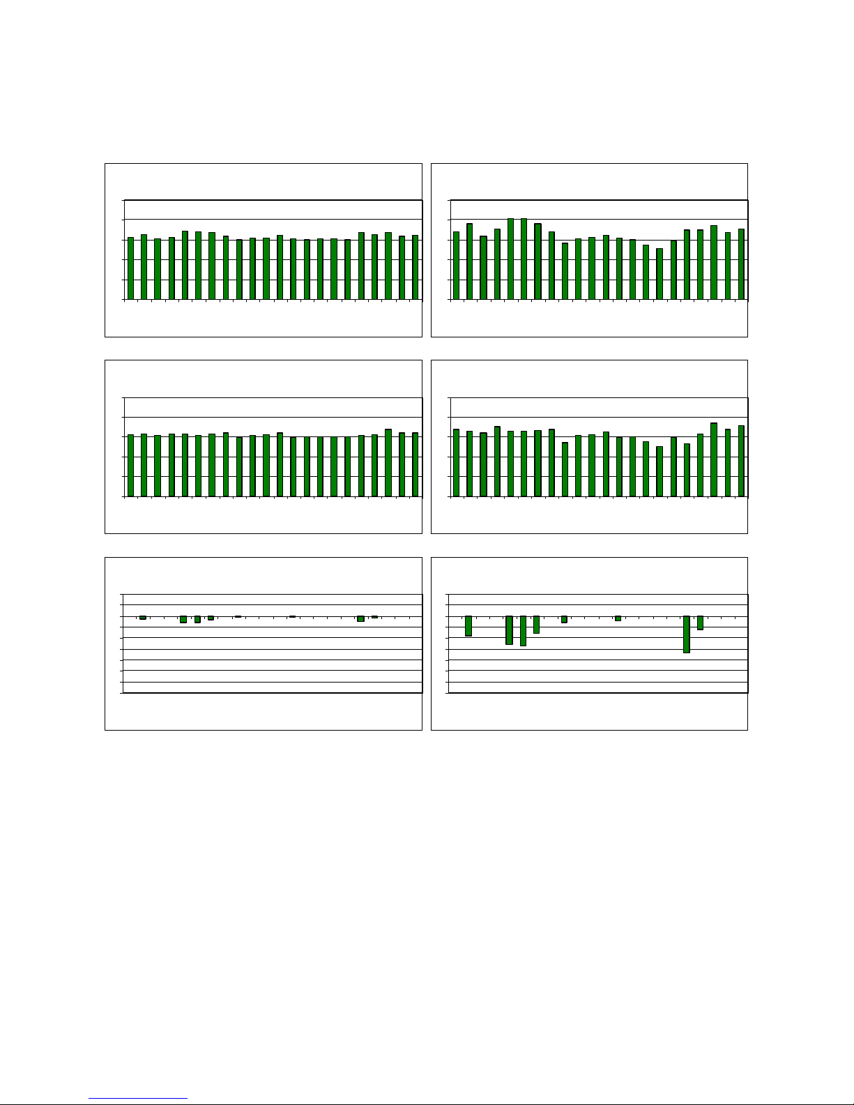
For small two-way systems (Figure 9-10), the main
improvement is seen at low frequencies in four out of
12 cases. In only one case is there is a significant improvement in the broadband flatness.
The broadband flatness of the two-way systems is improved in four (quartile data, Figure 11) or eight
Level, dB
5
4
3
2
1
0
-1
-2
-3
Subband M edia n Levels - All Models
LF MF HF LF MF HF
Original Equalised
(RMS data, Figure 12) cases out of 22. An equal
number of reductions and increases of low frequency
quartile values can be seen. MF subband quartile values improve in one case and deteriorate in 5 cases and
there are no changes in the HF subband. The flatness
in the broadband and LF subband of the RMS deviation data has improved indicating a reduction of outlier values. The MF and HF subbands show no
changes or a slight increase of the RMS deviation.
Three-way systems show a clear reduction in most
cases of both the quartile difference (Figure 13) and
RMS deviation (Figure 14) for the broadband and LF
subband. Slight, and equal numbers of, increases and
reductions are seen for MF and HF subbands.
A similar trend is seen for the three large systems included in this study (Figure 15-16). Mainly the LF
subband flatness is improved and this is also reflected
in the broadband improvement.
Some of the responses appeared to become worse in
the quartile difference and RMS deviation in the subband analysis. This was not reflected in the broadband
metrics, which indicates that the arbitrary subband frequency division introduced some of the error. Also,
the cases where this happened suffered from severe
anomalies within the pre-equalisation response due to
extremely bad room acoustic conditions. The equalisation was not designed to compensate for this.
Level, dB
5
4
3
2
1
0
-1
-2
-3
Subband Media n Levels - S ma ll models
LF MF HF LF MF HF
Original Equalised
Level, dB
5
4
3
2
1
0
-1
-2
-3
Subband Me dian Levels - 2-w ay models
LF MF HF LF MF HF
Original Equalised
Figure 3. Mean and standard deviation of subband median levels before and after equalisation.
The subband median levels (Figure 3) illustrate the
broadband frequency balance between the subbands.
Loudspeaker loading from nearby boundaries is re-
AES 23RD CONFERENCE, May 23-25, 2003 8
Level, dB
5
4
3
2
1
0
-1
-2
-3
Subband Median Le vels - 3-w ay m odels
LF MF HF LF MF HF
Original Equalised
flected in the LF subband median level before equalisation, especially in the often flush mounted threeway models. The median level in the LF subband is
Page 9

GOLDBERG AND MÄKIVIRTA AUTOMATED IN-SITU EQUALISATION
reduced after equalisation, which indicates that equalisation compensates well for the loudspeaker loading.
A better match across subbands of the average subband median level demonstrates that equalisation has
improved the broadband flatness. The largest improvement is seen in the three-way loudspeakers. In
the two-way systems the equalisation has improved
broadband flatness only marginally as the subband
median levels do not show major signs of change. The
broadband flatness improvement is mainly the result
of better alignment of the LF subband with the MF
Level, dB
1
0
Broadband LF MF HF
-1
-2
-3
Level, dB
1
0
Broadband LF MF HF
-1
-2
-3
25% to 75% Percentile Difference
Change due to Equa lisation - All models
25% to 75% Percentile Difference
Change due to Equalisa tion - Sma ll mode ls
and HF subbands. This indicates that the equalisation
has not only reduced the variation inside individual
subbands but also improved the broadband flatness of
the acoustical response, translating to a reduced
colouration of the audio at the listening position.
For all loudspeakers pooled together (Figure 3), the
equalisation reduces the variance in the median level
for the LF subband. A similar outcome is noted separately for each loudspeaker type. However, only in the
three-way systems is an improvement seen also in the
MF and HF subband variance.
Level, dB
1
0
-1
-2
-3
-4
-5
Level, dB
1
0
-1
-2
-3
-4
-5
Change due to Equalis ation - All mode ls
Broadband LF MF HF
Change due to Equalisa tion - Small m odels
Broadband LF MF HF
RMS Devi at ion
RMS Devi atio n
Level, dB
1
0
Broadband LF MF HF
-1
-2
-3
Level, dB
1
0
Broadband LF MF HF
-1
-2
-3
25% to 75% Percentile Difference
Change due to Equalis ation - 2-w ay models
25% to 75% Percentile Difference
Change due to Equalis ation - 3-w ay models
Level, dB
1
0
-1
-2
-3
-4
-5
Level, dB
1
0
-1
-2
-3
-4
-5
Change due to Equalisa tion - 2 -w ay models
Broadband LF MF HF
Change due to Equalisation - 3-wa y m odels
Broadband LF MF HF
RMS Devi at ion
RMS Devi atio n
Figure 4. Change in sound level deviation due to equalisation. For each subband, quartile difference and RMS deviation from the median. The error bar indicates the standard deviation.
AES 23RD CONFERENCE, May 23-25, 2003 9
Page 10

GOLDBERG AND MÄKIVIRTA AUTOMATED IN-SITU EQUALISATION
In Figure 4 the results are pooled for all products and
for each product type, excluding the main monitors
where there were only three cases. The change in
quartile difference and RMS deviation for the broadband and the subbands is illustrated. For all models,
the broadband flatness is improved by 0.4 dB and the
mean reduction in the LF subband RMS deviation is
1.4 dB. The RMS deviation for all models pooled together has been reduced by equalisation and the largest reduction is seen for the three-way systems. To
some extent this is similar for the quartile difference
but the small two-way and two-way systems do not
see such large improvements due to equalisation. This
indicates that the improvement is mainly a reduction
of extreme magnitude values (heights of peaks and
notches) in the low frequency response.
5. DISCUSSION
The objective of this paper is to present an automated
system for choosing appropriate room response control settings once an in-situ frequency response measurement has been made and to show that it is effective.
The room response controls in active loudspeakers
implement discrete filter parameter values rather than
a continuous parameter value range. The number of
possible filter parameter value combinations can be
quite large and so even an experienced operator can
find it difficult to choose the optimal settings.
The task of the automated optimiser is to find the optimal combination from the possible combinations of
discrete filter parameter values. The cost of performing a brute force search of all value combinations and
then choosing the best among them is prohibitive in
terms of computer processing time. The approach chosen is to exploit the heuristics of experienced calibration engineers and to reduce the number of alternatives by dividing the task into subsections that can reliably be solved independently. A significant part of
the heuristics is the order in which these choices
should be taken. A considerable improvement in the
speed of optimisation was achieved relative to a full
exhaustive search.
The optimisation algorithm is relatively robust to a
wide variety of situations, such as varying room
acoustics, different sized loudspeakers with differing
anechoic responses and varying in-situ responses [41].
The optimisation is efficient and so the software is fast
enough to be used routinely at in-situ loudspeaker
calibrations.
A case study demonstrates the statistical changes due
to the optimisation algorithm’s recommended room
response control settings. The settings achieve improved equalisation in the form of a smaller RMS de-
viation from the target response. The improvement is
not limited by the optimisation method but by the
room response controls which are not intended to correct for narrow-band deviations in the frequency response. Examples of these are response variations resulting from acoustic issues such as cancellations associated comb filtering due to reflections. These
should be solved acoustically rather than electronically.
The statistical analysis of 63 loudspeakers shows that
the automated equalisation is able to systematically
reduce the variability in the equalised responses and to
improve the frequency response flatness relative to the
target response. It achieves this by improving the
broadband frequency balance relative to the target response and by reducing the variability in the response,
particularly in the low frequencies. Across all loudspeaker groups the main improvement is in the reduction of extreme (outlier) values in the low frequency
band of the response.
It is interesting to note that the most commonly used
room response control was the midrange level, followed closely by the treble level and bass tilt control.
This is explained by the fact that the algorithm in most
stages minimises the RMS deviation, and in so doing
affects most efficiently the extreme deviations from
the median level.
For all models pooled together, the broadband flatness
was improved by equalisation. This improvement is
mainly due to a reduction of the extreme magnitude
values (heights of peaks and notches) in the low frequency response (LF subband).
The lack of improvement in the quartile values and
RMS deviation in the midrange and high frequencies
(MF and HF subbands) is because the room related
response variation becomes narrow band. Some improvement in the equalisation could be obtained with
room response controls offering a tilting or shaping of
the response within the mid-to-high frequency range.
The largest variability of the improvement in the low
frequency range can be explained by the acoustics
found in listening rooms [42]. At low frequencies the
radiation from the loudspeaker can be considered omnidirectional and the sound field in the room is usually
not very diffuse. This results in strong room effects
and hence large variations in the magnitude response
at these frequencies.
The largest improvement is seen for the three-way
systems and can be explained by two main factors.
Firstly, the rooms in which this type of loudspeaker is
typically installed are of a higher quality acoustical
design, so the sound field in them is well controlled.
Conversely, smaller loudspeakers are often installed in
rooms with little or no acoustical design, making cor-
AES 23RD CONFERENCE, May 23-25, 2003 10
Page 11

GOLDBERG AND MÄKIVIRTA AUTOMATED IN-SITU EQUALISATION
rections to the response by equalisation a very challenging task. Secondly, the three-way systems contain
more room response controls than the two-way systems, which gives a higher capability for the equaliser
to compensate for room problems. It should also be
noted that the type of equalisation the room response
controls are designed for is a gentle shaping of the response. High order narrow band corrections are not
possible, therefore the characteristics of the room and
the quality of its acoustical design will play a major
role.
6. CONCLUSIONS
The low-order room response adjustment filters in active loudspeakers can significantly improve the perceived quality of audio reproduction. The automated
optimisation algorithm presented in this paper is used
to select the optimal combination of settings for loudspeakers where the room response equaliser is implemented as a filter set with discrete parameter values.
The algorithm proves to be useful because it performs
systematically with widely varying types of loudspeakers, with slightly differing filter sets and loudspeakers found in multiple types of installations. The
efficiency and reliability of the algorithm has been
achieved by exploiting heuristics of experienced
sound system calibration engineers. The automated
methodology obtains systematically and consistently
the best combination of available filters, and performs
quickly irrespective of the operator. The algorithm has
been implemented in a loudspeaker calibration tool
used by specialists who set up and tune studios and
listening rooms.
7. ACKNOWLEDGEMENTS
The authors would like to thank Mr. Steve Fisher
(SCV London) for the original inspirational idea and
some of the measurements used in the statistical
analysis, Mr. Olli Salmensaari (Finnish Broadcasting
Corporation) for additional measurements, Mr. Lars
Morset (Morset Sound Development) and Genelec
Oy. Parts of this work are presented in more detail as
an MSc Thesis at the Helsinki University of Technology [41].
8. REFERENCES
[1] Genelec Oy, http://www.genelec.com (2003
Feb.).
[2] Walker R., “Equalisation of Room Acoustics
and Adaptive Systems in the Equalisation of Small
Rooms Acoustics,” Proc. 15th Int. Conf., paper 15005 (1998 Oct.).
[3] Cox T. J. and D’Antonio P., “Determining Optimum Room Dimensions for Critical Listening Environments: A New Methodology,” presented in 110th
Conv. Audio Eng. Soc., preprint 5353 (2001 May).
[4] Boner C. P. and Boner C. R., “Minimising
Feedback in Sound Systems and Room Ring Modes
with Passive Networks,” J. Acoust. Soc. America, vol.
37, pp. 131-135 (1965 Jan).
[5] Holman T., “New Factors in Sound for Cinema and Television,” J. Audio Eng. Soc., vol. 39, pp.
529-539 (1991 Jul/Aug.).
[6] Schulein R. B., “In-Situ Measurement and
Equalisation of Sound Reproduction Systems,” J. Au-
dio Eng. Soc., vol. 23, pp. 178-186 (1975 Apr.).
[7] Staffeldt H. and Rasmussen E., “The Subjectively Perceived Frequency Response in a Small and
Medium Sized Rooms,” SMPTE J., vol. 91, pp. 638643 (1982 Jul.).
[8] JBL, http://www.jblpro.com (2003 Feb.).
[9] Geddes E. R., “Small Room Acoustics in the
Statistical Region,” Proc. 15th Int. Conf., pp. 51-59
(1998 Sep.).
[10] Greiner R. A. and Schoessow M., “Design Aspects of Graphic Equalisers,” J. Audio Eng. Soc., vol.
31, pp. 394-407 (1983 Jun.).
[11] Bohn D.A., “Constant-Q Graphic Equalisers,”
J. Audio Eng. Soc., vol. 34, pp. 611-626 (1986 Sep.).
[12] Bohn D.A., “Operator Adjustable Equalisers:
An Overview,” Proc. 6th Int. Conf., paper 6-025
(1988 Apr.).
[13] “Motion Pictures– Dubbing Theatres, Review
Rooms and Indoor Theatres– B-Chain Electroacoustic
Response,” ANSI/SMPTE standard no 202M-1998
(1998).
[14] Genereux R., “Signal Processing Considerations for Acoustic Environment Correction,” Proc.
UK Conf. 1992, paper DSP-14 (1992 Sep.).
[15] Elliott S. J. and Nelson P. A., “Multiple Point
Equalisation in a Room Using Adaptive Digital Filters,” J. Acoustical Eng. Soc., vol. 37 (1989 Nov.).
[16] Karjalainen M., Piirilä E, Järvinen A. and Huopaniemi J., “Comparison of Loudspeaker Equalisation Methods Based on DSP Techniques,” J. Audio
Eng. Soc., vol. 47, pp. 14-31 (1999 Jan/Feb.).
[17] Neely S. T. and Allen J. B., “Invertability of a
Room Impulse Response,” J. Acoustical Soc. Amer-
ica, vol. 66, pp. 165-169 (1979 Jul.).
[18] Kirkeby O. and Nelson P.A., “Digital Filter
Design for Inversion Problems in Sound Reproduction,” J. Audio Eng. Soc., vol. 47, pp. 583-595 (1999
Jul/Aug.).
AES 23RD CONFERENCE, May 23-25, 2003 11
Page 12

GOLDBERG AND MÄKIVIRTA AUTOMATED IN-SITU EQUALISATION
[19] Radlovic B. D. and Kennedy R. A., “Nonminimum Phase Equalisation and its Subjective Importance in Room Acoustics,” IEEE Trans. Speech
Audio Proc., vol. 8, pp. 728-737 (2000 Nov.).
[20] Nelson P. A., Orduna-Bustamante F. and
Hamada H., “Inverse Filter Design and Equalisation
Zones in Multichannel Sound Reproduction,” IEEE
Trans. Speech Audio Proc., vol. 3, pp. 185-192 (1995
May).
[21] Kirkeby O., Nelson P.A., Hamada H., OrdunaBustamante F., “Fast Deconvolution of Multichannel
Systems Using Regularisation,” IEEE Trans. Speech
Audio Proc., vol. 6, pp. 189-194 (1998 Mar).
[22] Johansen L. G. and Rubak P., “Listening Test
Results from a new Loudspeaker/Room Correction
System,” presented in 110th Conv. Audio Eng. Soc.,
preprint 5323 (2001 May).
[23] Johansen L. G. and Rubak P., “Design and
Evaluation of Digital Filters Applied to Loudspeaker/Room Equalisation,” presented in 108th
Conv. Audio Eng. Soc., preprint 5172 (2000 Feb.).
[24] Fielder L. D., “Analysis of Traditional and
Reverberation-Reducing Methods of Room Equalisation,” J. Audio Eng. Soc., vol. 51, pp. 3-26 (2003
Jan/Feb.).
[25] Nelson P. A. and Elliott S. J., Active Control of
Sound (Academic Press, London, 1993).
[26] Darlington P. and Avis M. R., “Time Frequency Response of a Room with Active Acoustic
Absorption,” presented in 100th Conv. Audio Eng.
Soc., preprint 4192 (1996 May).
[27] Avis M. R., The Active Control of Low Fre-
quency Room Modes (Ph.D. Thesis, University of Salford, Dep. Applied Acoustics, 2001).
[28] Avis M. R., “IIR Bi-Quad Controllers for Low
Frequency Acoustic Resonance,” presented in 111th
Conv. Audio Eng. Soc., preprint 5474 (2001 Sep.).
[29] Mäkivirta A., Antsalo P. Karjalainen M. and
Välimäki V., “Low Frequency Modal Equalisation of
Loudspeaker Room-Responses,” presented in 111th
Conv. Audio Eng. Soc., preprint 5480 (2001 Sept.).
[30] Karjalainen M., Esquef P. A. A., Antsalo P.,
Mäkivirta A. and Välimäki V. “Frequency-Zooming
ARMA Modelling of Resonant and Reverberant Systems,” J. Audio Eng. Soc., vol. 50, pp. 1012-1029
(2002 Dec.).
[31] Moore B. C .J., Glasberg B. R., Plack C. J. and
Biswas A. K., “The shape of the Ear’s Temporal Window,” J. Acoustical Soc. America, vol. 83, pp. 11021116 (1988 Mar).
[32] Martikainen I., Varla A. and Partanen T., “Design of a High Power Active Control Room Monitor,”
presented at 86th Audio Engineering Society Convention, preprint 2755 (1989 Mar.).
[33] Allison R. F., “The Influence of Room
Boundaries on Loudspeaker Power Output,” J. Audio
Eng. Soc., vol. 22, pp. 314-320 (1974 June).
[34] Beranek L. L., Acoustics (Acoustical Society
of America, 1993).
[35] Kinsler L. E., Frey A. R., Coppins A. B. and
Sanders J. V., Fundamentals of Acoustics (3. ed., John
Wiley and Sons, 1982).
[36] Borwick J., Loudspeaker and Headphone
Handbook (2. ed., Focal Press, 1994).
[37] The MathWorks, “MATLAB Optimisation
Toolbox User’s Guide (v. 6.1)” (The MathWorks Inc.,
Natick, 2001).
[38] Goldberg A. P., Mäkivirta A., “Automated In-
Situ Frequency Response Optimisation of Active
Loudspeakers” accepted for 114th Conv. Audio Eng.
Soc. (2003 Mar.).
[39] Morset Sound Development, WinMLS2000,
http://www.winmls.com (2003 Feb.).
[40] NTI AG., Neutrik Test Instruments, 3382 Microphone, http://www.nt-instruments.com (2003
Feb.).
[41] Goldberg A. P., “In-Situ Frequency Response
Optimisation of Active Loudspeakers” (M.Sc. Thesis,
Helsinki University of Technology, Department of
Acoustics and Audio Signal Processing, 2003).
[42] Mäkivirta A., Anet C., “A Survey Study of In-
Situ Stereo and Multi-Channel Monitoring Conditions” presented in 111th Conv. Audio Eng. Soc.
(2001 Dec.).
AES 23RD CONFERENCE, May 23-25, 2003 12
Page 13

GOLDBERG AND MÄKIVIRTA AUTOMATED IN-SITU RESPONSE OPTIMISATION
APPENDIX A – SOFTWARE FLOW CHART
START
START
DIPtimiser
Display GUI
Reset GUI
Variables and
Graph
Add Supported
Models
Stored
Measurement
Stored
Measurement
Await User
Inputs
Reset Graph
and Outputs
Get Model
Number
Load Impulse
Response
Remove DC,
Window, FFT
and Smooth
Apply Mic
Compensation
Display
Original Freq
Response
Calculate
Target Resp
CLOSE
CLOSE
DIPtimiser
Model
Database
CTRL+M
Measurement
Dump
Microphone
Compensation
Figure 5. Software flow chart, part 1.
AES 23RD CONFERENCE, May 23-25, 2003 13
Display Target
Response
Set Frequency
Set DIPtimisation
Range
Range
12
Page 14

GOLDBERG AND MÄKIVIRTA AUTOMATED IN-SITU EQUALISATION
YNN
Y
12
Load Filters
Preset BRO
Is Large
System?
Find ML-TL
Ratio
Is Sma ll
System?
Set BL & BT
(wrt ML&TL)
Reset BRO
Model Filters
Set BT
Figure 5 continued. Software flow chart, part 2.
Is 3-way
System?
Set TT
Display Final
Tone Control
Settings
Display Final
Frequency
Response
AES 23RD CONFERENCE, May 23-25, 2003 14
Page 15

GOLDBERG AND MÄKIVIRTA AUTOMATED IN-SITU EQUALISATION
APPENDIX B – SOFTWARE GRAPHICAL USER INTERFACE
Figure 6. Software graphical user interface at start up.
AES 23RD CONFERENCE, May 23-25, 2003 15
Page 16

GOLDBERG AND MÄKIVIRTA AUTOMATED IN-SITU EQUALISATION
APPENDIX C – CASE EXAMPLE, STATISTICAL GRAPHS
Figure 7. Case example, optimisation results.
Figure 8. Case example, statistical output.
AES 23RD CONFERENCE, May 23-25, 2003 16
Page 17

GOLDBERG AND MÄKIVIRTA AUTOMATED IN-SITU EQUALISATION
APPENDIX D – STATISTICAL GRAPHS
Level, dB
12
10
8
6
4
2
0
Broadband 25% to 75% Percentile
Differ ence Befor e Equalis ation
1029A
1029A
1029A
1029A
1029A
1029A
1029A
1029A
1029A
1029A
1029A
Level, dB
12
10
8
6
4
2
0
1029A
Low Frequency 25% to 75% Percentile
Difference Before Equalisation
1029A
1029A
1029A
1029A
1029A
1029A
1029A
1029A
1029A
1029A
1029A
1029A
Level, dB
12
10
8
6
4
2
0
Level, dB
0.5
0.0
-0.5
-1.0
-1.5
-2.0
-2.5
-3.0
-3.5
-4.0
-4.5
Broadband 25% to 75% Percentile
Difference After Equalisation
1029A
1029A
1029A
1029A
1029A
1029A
1029A
Broadband 25% to 75% Percentile
Difference Change due to Equalisation
1029A
1029A
1029A
1029A
1029A
1029A
1029A
1029A
1029A
1029A
1029A
1029A
1029A
1029A
1029A
1029A
1029A
Level, dB
12
10
8
6
4
2
0
Level, dB
0.5
0.0
-0.5
-1.0
-1.5
-2.0
-2.5
-3.0
-3.5
-4.0
-4.5
1029A
1029A
Figure 9a. 25% to 75% percentile differences for small 2-way systems.
Low Frequency 25% to 75% Percentile
Difference After Equalisation
1029A
1029A
1029A
1029A
1029A
1029A
1029A
1029A
Low Frequency 25% to 75% Percentile
Differ ence Change due to Equalisation
1029A
1029A
1029A
1029A
1029A
1029A
1029A
1029A
1029A
1029A
1029A
1029A
1029A
1029A
AES 23RD CONFERENCE, May 23-25, 2003 17
Page 18

GOLDBERG AND MÄKIVIRTA AUTOMATED IN-SITU EQUALISATION
Level, dB
12
10
8
6
4
2
0
1029A
Midra nge 25 % to 75% Perc entile
Difference Before Equalisation
1029A
1029A
1029A
1029A
1029A
1029A
1029A
1029A
1029A
1029A
Level, dB
12
10
8
6
4
2
0
1029A
High Frequency 25% to 75% Percentile
Differ ence Befor e Equalisation
1029A
1029A
1029A
1029A
1029A
1029A
1029A
1029A
1029A
1029A
1029A
1029A
Level, dB
12
10
8
6
4
2
0
Level, dB
0.5
0.0
-0.5
-1.0
-1.5
-2.0
-2.5
-3.0
-3.5
-4.0
-4.5
1029A
Midra nge 25 % to 75% Perc entile
Difference After Equalisation
1029A
1029A
1029A
1029A
1029A
1029A
Midrange 25% to 75% Percentile
Difference Change due to Equalisation
1029A
1029A
1029A
1029A
1029A
1029A
1029A
1029A
1029A
1029A
1029A
1029A
1029A
1029A
1029A
1029A
1029A
Level, dB
12
10
8
6
4
2
0
Level, dB
0.5
0.0
-0.5
-1.0
-1.5
-2.0
-2.5
-3.0
-3.5
-4.0
-4.5
1029A
1029A
1029A
Figure 9b. 25% to 75% percentile differences for small 2-way systems.
High Frequency 25% to 75% Percentile
Difference After Equalisation
1029A
1029A
1029A
1029A
1029A
1029A
1029A
High Frequenc y 25 % to 75% Perce ntile
Differ ence Change due to Equalisation
1029A
1029A
1029A
1029A
1029A
1029A
1029A
1029A
1029A
1029A
1029A
1029A
1029A
1029A
AES 23RD CONFERENCE, May 23-25, 2003 18
Page 19

GOLDBERG AND MÄKIVIRTA AUTOMATED IN-SITU EQUALISATION
Level, dB
10
8
6
4
2
0
1029A
Broadba nd RMS De via t ion
Before Equalis ation
1029A
1029A
1029A
1029A
1029A
1029A
1029A
1029A
1029A
1029A
1029A
Level, dB
10
8
6
4
2
0
1029A
Low Freque ncy RMS Deviation
Before Equalis ation
1029A
1029A
1029A
1029A
1029A
1029A
1029A
1029A
1029A
1029A
1029A
Level, dB
10
8
6
4
2
0
Level, dB
2
1
0
-1
-2
-3
-4
-5
-6
-7
1029A
1029A
Broadba nd RMS De via t ion
After Equalisation
1029A
1029A
1029A
1029A
Broadband RMS Deviation
Change due to Equalisation
1029A
1029A
1029A
1029A
1029A
1029A
1029A
1029A
1029A
1029A
1029A
1029A
1029A
1029A
1029A
1029A
Figure 10a. RMS deviation for small 2-way systems.
1029A
1029A
Level, dB
10
8
6
4
2
0
Level, dB
2
1
0
-1
-2
-3
-4
-5
-6
-7
1029A
1029A
Low Freque ncy RMS Deviation
After Equalisation
1029A
1029A
1029A
1029A
1029A
Low Freque ncy RMS Deviation
Change due to Equalisation
1029A
1029A
1029A
1029A
1029A
1029A
1029A
1029A
1029A
1029A
1029A
1029A
1029A
1029A
1029A
1029A
1029A
AES 23RD CONFERENCE, May 23-25, 2003 19
Page 20

GOLDBERG AND MÄKIVIRTA AUTOMATED IN-SITU EQUALISATION
Level, dB
10
8
6
4
2
0
1029A
Midrange RM S Devia tion
Befor e Equalisation
1029A
1029A
1029A
1029A
1029A
1029A
1029A
1029A
1029A
1029A
1029A
Level, dB
10
8
6
4
2
0
1029A
High Freque ncy RMS Deviation
Before Equalisation
1029A
1029A
1029A
1029A
1029A
1029A
1029A
1029A
1029A
1029A
1029A
Level, dB
10
8
6
4
2
0
Level, dB
2
1
0
-1
-2
-3
-4
-5
-6
-7
1029A
1029A
Midrange RM S Devia tion
After Equalisation
1029A
1029A
1029A
1029A
Midrange RM S Devia tion
Change due to Equalisation
1029A
1029A
1029A
1029A
1029A
1029A
1029A
1029A
1029A
1029A
1029A
1029A
1029A
1029A
1029A
1029A
Figure 10b. RMS deviation for small 2-way systems.
1029A
1029A
Level, dB
10
8
6
4
2
0
Level, dB
2
1
0
-1
-2
-3
-4
-5
-6
-7
1029A
1029A
High Freque ncy RMS Deviation
After Equalisation
1029A
1029A
1029A
1029A
1029A
High Freque ncy RMS Deviation
Change due to Equalisation
1029A
1029A
1029A
1029A
1029A
1029A
1029A
1029A
1029A
1029A
1029A
1029A
1029A
1029A
1029A
1029A
1029A
AES 23RD CONFERENCE, May 23-25, 2003 20
Page 21

GOLDBERG AND MÄKIVIRTA AUTOMATED IN-SITU EQUALISATION
Level, dB
12
10
8
6
4
2
0
1030A
Broadband 2 5% to 75 % Perc entile
Difference Before Equalisation
1030A
1031A
1031A
1031A
1031A
1031A
1031A
1031A
1032A
Level, dB
12
10
8
6
4
2
0
1032A
Low Frequency 25% to 75% Perce ntile
Differ ence Befor e Equalisation
1030A
1030A
1031A
1031A
1031A
1031A
1031A
1031A
1031A
1032A
1032A
Level, dB
12
10
8
6
4
2
0
1030A
Level, dB
0.5
0.0
-0.5
-1.0
-1.5
-2.0
-2.5
-3.0
-3.5
-4.0
-4.5
Broadband 2 5% to 75 % Perc entile
Differ ence After Equalis ation
1030A
1031A
1031A
1031A
1031A
Broadband 2 5% to 75 % Perc entile
Difference Change due to Equalisation
1030A
1030A
1031A
1031A
1031A
1031A
1031A
1031A
1031A
1031A
1031A
1031A
1032A
1032A
1032A
1032A
Level, dB
12
10
8
6
4
2
0
1030A
Level, dB
0.5
0.0
-0.5
-1.0
-1.5
-2.0
-2.5
-3.0
-3.5
-4.0
-4.5
Figure 11a. 25% to 75% percentile differences for 2-way systems.
Low Frequency 25% to 75% Perce ntile
Differ ence Afte r Equalisa tion
1030A
1031A
1031A
1031A
1031A
Low Frequency 2 5% t o 7 5 % P er ce nt i le
Differ ence Change due to Equalisation
1030A
1030A
1031A
1031A
1031A
1031A
1031A
1031A
1031A
1031A
1031A
1031A
1032A
1032A
1032A
1032A
AES 23RD CONFERENCE, May 23-25, 2003 21
Page 22

GOLDBERG AND MÄKIVIRTA AUTOMATED IN-SITU EQUALISATION
Level, dB
12
10
8
6
4
2
0
1030A
Midra nge 25 % to 75% Percentile
Difference Before Equalisation
1030A
1031A
1031A
1031A
1031A
1031A
1031A
1031A
1032A
Level, dB
12
10
8
6
4
2
0
1032A
High Frequency 25% to 75% Percentile
Differ ence Befor e Equalisation
1030A
1030A
1031A
1031A
1031A
1031A
1031A
1031A
1031A
1032A
1032A
Level, dB
12
10
8
6
4
2
0
1030A
Level, dB
0.5
0.0
-0.5
-1.0
-1.5
-2.0
-2.5
-3.0
-3.5
-4.0
-4.5
1030A
Midra nge 25 % to 75% Percentile
Difference After Equalisation
1030A
1031A
1031A
1031A
1031A
1031A
1031A
Midrange 25% to 75% Percentile
Difference Change due to Equalisation
1030A
1031A
1031A
1031A
1031A
1031A
1031A
1031A
1031A
1032A
1032A
1032A
1032A
Level, dB
12
10
8
6
4
2
0
1030A
Level, dB
0.5
0.0
-0.5
-1.0
-1.5
-2.0
-2.5
-3.0
-3.5
-4.0
-4.5
Figure 11b. 25% to 75% percentile differences for 2-way systems.
High Frequency 25% to 75% Percentile
Differ ence After Equalisation
1030A
1031A
1031A
1031A
1031A
High Frequenc y 25 % to 75% Percentile
Differ ence Change due to Equalisation
1030A
1030A
1031A
1031A
1031A
1031A
1031A
1031A
1031A
1031A
1031A
1031A
1032A
1032A
1032A
1032A
AES 23RD CONFERENCE, May 23-25, 2003 22
Page 23
GOLDBERG AND MÄKIVIRTA AUTOMATED IN-SITU EQUALISATION
Level, dB
10
8
6
4
2
0
1030A
Broadband RMS Deviation
Before Equalis ation
1030A
1031A
1031A
1031A
1031A
1031A
1031A
1031A
1032A
1032A
Level, dB
10
8
6
4
2
0
1030A
Low Frequency RMS Deviation
Before Equalisation
1030A
1031A
1031A
1031A
1031A
1031A
1031A
1031A
1032A
1032A
Level, dB
10
8
6
4
2
0
1030A
Level, dB
2
1
0
-1
-2
-3
-4
-5
-6
-7
1030A
Broadband RMS Deviation
After Equalis ation
1030A
1031A
1031A
1031A
Broadband RMS Deviation
Change due to Equalisation
1030A
1031A
1031A
1031A
1031A
1031A
1031A
1031A
1031A
1031A
1031A
1031A
Figure 12a. RMS deviation for 2-way systems.
1032A
1032A
1032A
1032A
Level, dB
10
8
6
4
2
0
1030A
Level, dB
2
1
0
-1
-2
-3
-4
-5
-6
-7
1030A
Low Frequency RMS Deviation
After Equalisation
1030A
1031A
1031A
1031A
1031A
Low Frequency RMS Deviation
Change due to Equalisation
1030A
1031A
1031A
1031A
1031A
1031A
1031A
1031A
1031A
1031A
1031A
1032A
1032A
1032A
1032A
AES 23RD CONFERENCE, May 23-25, 2003 23
Page 24

GOLDBERG AND MÄKIVIRTA AUTOMATED IN-SITU EQUALISATION
Level, dB
10
8
6
4
2
0
1030A
Midrange RM S Devia tion
Befor e Equalisation
1030A
1031A
1031A
1031A
1031A
1031A
1031A
1031A
1032A
1032A
Level, dB
10
8
6
4
2
0
1030A
High Freque ncy RMS Deviation
Before Equalisation
1030A
1031A
1031A
1031A
1031A
1031A
1031A
1031A
1032A
1032A
Level, dB
10
8
6
4
2
0
1030A
Level, dB
2
1
0
-1
-2
-3
-4
-5
-6
-7
1030A
1030A
Midrange RM S Devia tion
After Equalisation
1030A
1031A
1031A
1031A
Midrange RM S Devia tion
Change due to Equalisation
1031A
1031A
1031A
1031A
1031A
1031A
1031A
1031A
1031A
1031A
1031A
Figure 12b. RMS deviation for 2-way systems.
1032A
1032A
1032A
1032A
Level, dB
10
8
6
4
2
0
1030A
Level, dB
2
1
0
-1
-2
-3
-4
-5
-6
-7
1030A
High Freque ncy RMS Deviation
After Equalisation
1030A
1031A
1031A
1031A
1031A
High Freque ncy RMS Deviation
Change due to Equalisation
1030A
1031A
1031A
1031A
1031A
1031A
1031A
1031A
1031A
1031A
1031A
1032A
1032A
1032A
1032A
AES 23RD CONFERENCE, May 23-25, 2003 24
Page 25

GOLDBERG AND MÄKIVIRTA AUTOMATED IN-SITU EQUALISATION
Level, dB
12
10
8
6
4
2
0
S30D
Broadband 2 5% to 75 % Perc entile
Difference Before Equalisation
S30D
S30D
S30D
1037B
1037B
1037B
1037B
1037B
1038A
1038A
1038A
1038A
1038A
Level, dB
12
10
8
6
4
2
0
1039A
Low Frequency 25% to 75% Perce ntile
Differ ence Befor e Equalisation
S30D
S30D
S30D
S30D
1037B
1037B
1037B
1037B
1037B
1038A
1038A
1038A
1038A
1038A
1039A
Level, dB
12
10
8
6
4
2
0
S30D
Level, dB
0.5
0.0
-0.5
-1.0
-1.5
-2.0
-2.5
-3.0
-3.5
-4.0
-4.5
Broadband 2 5% to 75 % Perc entile
Differ ence After Equalis ation
S30D
S30D
S30D
1037B
1037B
1037B
1037B
Broadband 2 5% to 75 % Perc entile
Difference Change due to Equalisation
S30D
S30D
S30D
S30D
1037B
1037B
1037B
1037B
1037B
1037B
1038A
1038A
1038A
1038A
1038A
1038A
1038A
1038A
1038A
Level, dB
12
10
8
6
4
2
0
1039A
1038A
1039A
S30D
Level, dB
0.5
0.0
-0.5
-1.0
-1.5
-2.0
-2.5
-3.0
-3.5
-4.0
-4.5
Figure 13a. 25% to 75% percentile differences for 3-way systems.
Low Frequency 25% to 75% Perce ntile
Differ ence Afte r Equalisa tion
S30D
S30D
S30D
1037B
1037B
1037B
1037B
Low Frequency 25% to 75% Perce ntile
Differ ence Change due to Equalisation
S30D
S30D
S30D
S30D
1037B
1037B
1037B
1037B
1037B
1037B
1038A
1038A
1038A
1038A
1038A
1038A
1038A
1038A
1038A
1038A
1039A
1039A
AES 23RD CONFERENCE, May 23-25, 2003 25
Page 26

GOLDBERG AND MÄKIVIRTA AUTOMATED IN-SITU EQUALISATION
Level, dB
12
10
8
6
4
2
0
S30D
Midra nge 25 % to 75% Perc entile
Difference Before Equalisation
S30D
S30D
S30D
1037B
1037B
1037B
1037B
1037B
1038A
1038A
1038A
1038A
1038A
Level, dB
12
10
8
6
4
2
0
1039A
High Frequency 25% to 75% Percentile
Differ ence Befor e Equalisation
S30D
S30D
S30D
S30D
1037B
1037B
1037B
1037B
1037B
1038A
1038A
1038A
1038A
1038A
1039A
Level, dB
12
10
8
6
4
2
0
S30D
Level, dB
0.5
0.0
-0.5
-1.0
-1.5
-2.0
-2.5
-3.0
-3.5
-4.0
-4.5
Midra nge 25 % to 75% Perc entile
Difference After Equalisation
S30D
S30D
S30D
1037B
1037B
1037B
1037B
Midrange 25% to 75% Percentile
Difference Change due to Equalisation
S30D
S30D
S30D
S30D
1037B
1037B
1037B
1037B
1037B
1037B
1038A
1038A
1038A
1038A
1038A
1038A
1038A
1038A
1038A
1038A
1039A
1039A
Level, dB
12
10
8
6
4
2
0
S30D
Level, dB
0.5
0.0
-0.5
-1.0
-1.5
-2.0
-2.5
-3.0
-3.5
-4.0
-4.5
S30D
Figure 13b. 25% to 75% percentile differences for 3-way systems.
High Frequency 25% to 75% Percentile
Difference After Equalisation
S30D
S30D
S30D
1037B
1037B
1037B
1037B
1037B
1038A
High Frequenc y 25 % to 75% Perce ntile
Differ ence Change due to Equalisation
S30D
S30D
S30D
1037B
1037B
1037B
1037B
1037B
1038A
1038A
1038A
1038A
1038A
1038A
1038A
1038A
1038A
1039A
1039A
AES 23RD CONFERENCE, May 23-25, 2003 26
Page 27

GOLDBERG AND MÄKIVIRTA AUTOMATED IN-SITU EQUALISATION
Level, dB
10
8
6
4
2
0
S30D
S30D
Broadba nd RMS De via t ion
Before Equalis ation
S30D
S30D
1037B
1037B
1037B
1037B
1037B
1038A
1038A
1038A
1038A
1038A
1039A
Level, dB
10
8
6
4
2
0
S30D
Low Freque ncy RMS Deviation
Before Equalisation
S30D
S30D
S30D
1037B
1037B
1037B
1037B
1037B
1038A
1038A
1038A
1038A
1038A
1039A
Level, dB
10
8
6
4
2
0
S30D
Level, dB
2
1
0
-1
-2
-3
-4
-5
-6
-7
S30D
S30D
S30D
Broadba nd RMS De via t ion
After Equalisation
S30D
S30D
1037B
1037B
1037B
Broadband RMS Deviation
Change due to Equalisation
S30D
S30D
1037B
1037B
1037B
1037B
1037B
1037B
1038A
1038A
1038A
1037B
1038A
1038A
1038A
Figure 14a. RMS deviation for 3-way systems.
1038A
1038A
1038A
1038A
1039A
1039A
Level, dB
10
8
6
4
2
0
S30D
Level, dB
2
1
0
-1
-2
-3
-4
-5
-6
-7
S30D
Low Freque ncy RMS Deviation
After Equalisation
S30D
S30D
S30D
1037B
1037B
1037B
Low Freque ncy RMS Deviation
Change due to Equalisation
S30D
S30D
S30D
1037B
1037B
1037B
1037B
1037B
1037B
1037B
1038A
1038A
1038A
1038A
1038A
1038A
1038A
1038A
1038A
1038A
1039A
1039A
AES 23RD CONFERENCE, May 23-25, 2003 27
Page 28

GOLDBERG AND MÄKIVIRTA AUTOMATED IN-SITU EQUALISATION
Level, dB
10
8
6
4
2
0
S30D
Midrange RMS De viation
Before Equalisation
S30D
S30D
S30D
1037B
1037B
1037B
1037B
1037B
1038A
1038A
1038A
1038A
1038A
1039A
Level, dB
10
8
6
4
2
0
S30D
High Frequency RMS De viation
Befor e Equalis a t ion
S30D
S30D
S30D
1037B
1037B
1037B
1037B
1037B
1038A
1038A
1038A
1038A
1038A
1039A
Level, dB
10
8
6
4
2
0
S30D
Level, dB
2
1
0
-1
-2
-3
-4
-5
-6
-7
S30D
S30D
S30D
Midrange RMS De viation
After Equalisation
S30D
S30D
1037B
1037B
1037B
Midrange RMS De viation
Change due to Equalisation
S30D
S30D
1037B
1037B
1037B
1037B
1037B
1037B
1037B
1038A
1038A
1038A
1038A
1038A
1038A
Figure 14b. RMS deviation for 3-way systems.
1038A
1038A
1038A
1038A
1039A
1039A
Level, dB
10
8
6
4
2
0
S30D
Level, dB
2
1
0
-1
-2
-3
-4
-5
-6
-7
S30D
High Frequency RMS De viation
After Equalisation
S30D
S30D
S30D
1037B
1037B
1037B
High Frequency RMS De viation
Change due to Equalisation
S30D
S30D
S30D
1037B
1037B
1037B
1037B
1037B
1037B
1037B
1038A
1038A
1038A
1038A
1038A
1038A
1038A
1038A
1038A
1038A
1039A
1039A
AES 23RD CONFERENCE, May 23-25, 2003 28
Page 29

GOLDBERG AND MÄKIVIRTA AUTOMATED IN-SITU EQUALISATION
Level, dB
12
10
8
6
4
2
0
Broadband 25% to 75% Percentile
Difference Before Equalisation
Level, dB
12
10
8
6
4
2
0
Low Frequency 25% to 75% Percent ile
Difference Before Equalisation
Level, dB
12
10
8
6
4
2
0
Level, dB
0.5
0.0
-0.5
-1.0
-1.5
-2.0
-2.5
-3.0
-3.5
-4.0
-4.5
1036A
Broadband 25% to 75% Percentile
Difference After Equalisation
1036A
Broadband 25% to 75% Percentile
Difference Change due to Equalisation
1036A
1036A
1036A
1036A
1036A
1036A
1036A
Level, dB
12
10
8
6
4
2
0
Level, dB
0.5
0.0
-0.5
-1.0
-1.5
-2.0
-2.5
-3.0
-3.5
-4.0
-4.5
Figure 15a. 25% to 75% percentile differences for large systems.
1036A
1036A
Low Frequency 25% to 75% Percent ile
Difference After Equalisation
1036A
1036A
Low Frequency 25% to 75% Percent ile
Difference Change due to Equalisation
1036A
1036A
1036A
1036A
1036A
AES 23RD CONFERENCE, May 23-25, 2003 29
Page 30

GOLDBERG AND MÄKIVIRTA AUTOMATED IN-SITU EQUALISATION
Level, dB
12
10
8
6
4
2
0
Midrange 25% to 75% Percentile
Difference Before Equalisation
Level, dB
12
10
8
6
4
2
0
High Fr equenc y 25 % to 75% Perce ntile
Difference Before Equalisation
Level, dB
12
10
8
6
4
2
0
Level, dB
0.5
0.0
-0.5
-1.0
-1.5
-2.0
-2.5
-3.0
-3.5
-4.0
-4.5
1036A
Midrange 25% to 75% Percentile
Difference After Equalisation
1036A
Midrange 25% to 75% Percentile
Difference Change due to Equalisation
1036A
1036A
1036A
1036A
1036A
1036A
1036A
Level, dB
12
10
8
6
4
2
0
Level, dB
0.5
0.0
-0.5
-1.0
-1.5
-2.0
-2.5
-3.0
-3.5
-4.0
-4.5
Figure 15b. 25% to 75% percentile differences for large systems.
1036A
1036A
High Fr equenc y 25 % to 75% Perce ntile
Difference After Equalisation
1036A
1036A
High Frequency 25% to 75% Percentile
Differ ence Change due to Equalisa tion
1036A
1036A
1036A
1036A
1036A
AES 23RD CONFERENCE, May 23-25, 2003 30
Page 31

GOLDBERG AND MÄKIVIRTA AUTOMATED IN-SITU EQUALISATION
Level, dB
10
8
6
4
2
0
Broadba nd RMS De via t ion
Before Equalis ation
Level, dB
10
8
6
4
2
0
Low Freque ncy RMS Deviation
Before Equalis ation
Level, dB
10
8
6
4
2
0
Level, dB
2
1
0
-1
-2
-3
-4
-5
-6
-7
1036A
Broadba nd RMS De via t ion
After Equalisation
1036A
Broadband RMS Deviation
Change due to Equalisation
1036A
1036A
1036A
1036A
Figure 16a. RMS deviation for large systems.
1036A
1036A
1036A
Level, dB
10
8
6
4
2
0
Level, dB
2
1
0
-1
-2
-3
-4
-5
-6
-7
1036A
1036A
Low Freque ncy RMS Deviation
After Equalisation
1036A
1036A
Low Freque ncy RMS Deviation
Change due to Equalisation
1036A
1036A
1036A
1036A
1036A
AES 23RD CONFERENCE, May 23-25, 2003 31
Page 32

GOLDBERG AND MÄKIVIRTA AUTOMATED IN-SITU EQUALISATION
Level, dB
10
8
6
4
2
0
Midrange RMS De viation
Before Equalisation
Level, dB
10
8
6
4
2
0
High Frequency RMS De viation
Befor e Equalis a t ion
Level, dB
10
8
6
4
2
0
Level, dB
2
1
0
-1
-2
-3
-4
-5
-6
-7
1036A
Midrange RMS De viation
After Equalisation
1036A
Midrange RMS De viation
Change due to Equalisation
1036A
1036A
1036A
1036A
Figure 16b. RMS deviation for large systems.
1036A
1036A
1036A
Level, dB
10
8
6
4
2
0
Level, dB
2
1
0
-1
-2
-3
-4
-5
-6
-7
1036A
1036A
High Frequency RMS De viation
After Equalisation
1036A
1036A
High Frequency RMS De viation
Change due to Equalisation
1036A
1036A
1036A
1036A
1036A
AES 23RD CONFERENCE, May 23-25, 2003 32
 Loading...