

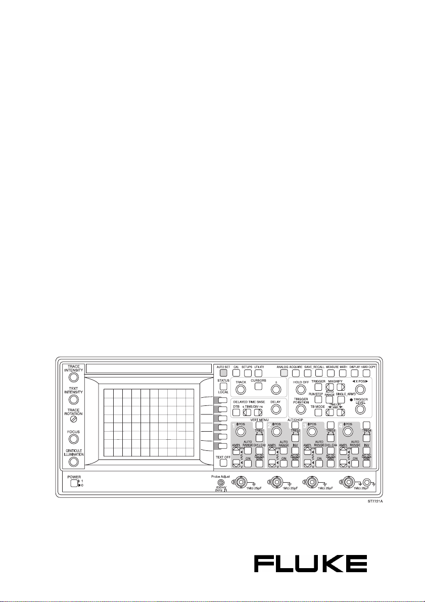
Page 1
$XWRUDQJLQJ
&RPEL6FRSH
,QVWUXPHQW
30%30%30%
30%30%
I
SCPI Users Manual
02/- Nov-1998
®
Page 2

II
TRADEMARKS
Microsoft, and Microsoft QuickBASIC are trademarks of Microsoft Corporation.
IBM is a registered trademark of International Business Machines Corporation.
CombiScope
PCIIA is a trademark of National Instruments Corporation.
HPGL is a trademark of Hewlett-Packard Company.
is a trademark of Fluke Corporation.
Copyright 1996, 1998 Fluke Corporation
All rights reserved. No part of this manual may be reproduced by any means or in
any form without written permission of the copyright owner.
Printed in the Netherlands
Page 3

CONTENTS Page
III
1 ABOUT THIS MANUAL
1.1 What this Manual Contains
. . . . . . . . . . . . . . . . . . . . . . . . . . . . . . . . 1-1
. . . . . . . . . . . . . . . . . . . . . . . . . . . . . . 1-1
2 GETTING STARTED WITH SCPI PROGRAMMING
2.1 Preparations for SCPI Programming
2.1.1 System setup . . . . . . . . . . . . . . . . . . . . . . . . . . . . . . . . . . . . 2-1
2.1.2 Programming environment . . . . . . . . . . . . . . . . . . . . . . . . . . 2-1
2.2 Initializing the CombiScope Instrument
2.2.1 How to reset the CombiScope instrument . . . . . . . . . . . . . . 2-4
2.2.2 How to identify the CombiScope instrument . . . . . . . . . . . . 2-4
2.2.3 How to switch between digital and analog mode . . . . . . . . . 2-4
2.3 Error Reporting
2.4 Acquiring Traces
2.4.1 How to acquire a single shot trace . . . . . . . . . . . . . . . . . . . . 2-7
2.4.2 How to acquire repetitive traces . . . . . . . . . . . . . . . . . . . . . . 2-8
2.5 Measuring Signal Characteristics
2.5.1 How to make a single shot measurement . . . . . . . . . . . . . 2-10
2.5.2 How to make repeated measurements . . . . . . . . . . . . . . . 2-10
. . . . . . . . . . . . . . . . . . . . . . . . . . . . . . . . . . . . . . . . 2-5
. . . . . . . . . . . . . . . . . . . . . . . . . . . . . . . . . . . . . . 2-6
. . . . . . . . . . . . . . . . . . . . . . 2-1
. . . . . . . . . . . . . . . . . . . . 2-4
. . . . . . . . . . . . . . . . . . . . . . . . . 2-9
. . 2-1
3 USING THE COMBISCOPE INSTRUMENTS
3.1 Introduction
3.2 Fundamental Programming Concepts
3.2.1 Measurement instructions . . . . . . . . . . . . . . . . . . . . . . . . . . 3-4
3.2.2 Single function progra mming using the instrument model . . 3-5
3.2.3 Instrument setup . . . . . . . . . . . . . . . . . . . . . . . . . . . . . . . . . 3-6
3.2.4 Front panel simulation . . . . . . . . . . . . . . . . . . . . . . . . . . . . . 3-7
. . . . . . . . . . . . . . . . . . . . . . . . . . . . . . . . . . . . . . . . . . . 3-1
. . . . . . . . . . . . . . . . . . . . . 3-3
. . . . . . . . . 3-1
Page 4

IV
3.3 Measuring Signal Characteristics . . . . . . . . . . . . . . . . . . . . . . . . . 3-8
3.3.1 The MEASure? query . . . . . . . . . . . . . . . . . . . . . . . . . . . . . 3-8
3.3.2 Benefits of using parameters . . . . . . . . . . . . . . . . . . . . . . . . 3-9
3.3.3 Waveform measurements . . . . . . . . . . . . . . . . . . . . . . . . . 3-11
3.3.4 Customizing settings . . . . . . . . . . . . . . . . . . . . . . . . . . . . . 3-13
3.3.5 Multiple measurements . . . . . . . . . . . . . . . . . . . . . . . . . . . 3-14
3.3.6 Multiple characteristics from a single acquisition. . . . . . . . 3-15
3.3.7 Trigger control via GPIB . . . . . . . . . . . . . . . . . . . . . . . . . . . 3-16
3.3.8 Fetching characteristics from memory traces . . . . . . . . . . 3-17
3.4 Acquisition . . . . . . . . . . . . . . . . . . . . . . . . . . . . . . . . . . . . . . . . . . 3-18
3.4.1 Acquisition control . . . . . . . . . . . . . . . . . . . . . . . . . . . . . . . 3-18
3.4.1.1 Triggering
3.4.1.2 Video triggering
3.4.1.3 The trigger modes
3.4.1.4 Pre- and post-triggering
3.4.1.5 External triggering
3.4.2 Reading trace acquisitions . . . . . . . . . . . . . . . . . . . . . . . . . 3-29
3.4.2.1 Single-shot acquisition
3.4.2.2 Repetitive acquisitions
3.4.3 Conversion of trace data . . . . . . . . . . . . . . . . . . . . . . . . . . 3-31
3.4.3.1 Conversion of 8-bit samples to integer
3.4.3.2 Conversion of 16-bit samples to integer
3.4.3.3 Conversion to voltage values
. . . . . . . . . . . . . . . . . . . . . . . . . . . . . . . . . . . 3-20
. . . . . . . . . . . . . . . . . . . . . . . . . . . . . . 3-23
. . . . . . . . . . . . . . . . . . . . . . . . . . . . 3-25
. . . . . . . . . . . . . . . . . . . . . . . . 3-27
. . . . . . . . . . . . . . . . . . . . . . . . . . . . 3-28
. . . . . . . . . . . . . . . . . . . . . . . . . 3-30
. . . . . . . . . . . . . . . . . . . . . . . . . 3-30
. . . . . . . . . . . . . 3-32
. . . . . . . . . . . . 3-33
. . . . . . . . . . . . . . . . . . . . 3-34
3.5 Averaging Acquisition Data . . . . . . . . . . . . . . . . . . . . . . . . . . . . 3-36
3.6 Channel Selection . . . . . . . . . . . . . . . . . . . . . . . . . . . . . . . . . . . . 3-38
3.7 Signal Conditioning . . . . . . . . . . . . . . . . . . . . . . . . . . . . . . . . . . . 3-39
3.7.1 AC/DC/ground coupling . . . . . . . . . . . . . . . . . . . . . . . . . . . 3-39
3.7.2 Input filtering . . . . . . . . . . . . . . . . . . . . . . . . . . . . . . . . . . . 3-40
3.7.3 Input impedance . . . . . . . . . . . . . . . . . . . . . . . . . . . . . . . . 3-40
3.7.4 Input polarity . . . . . . . . . . . . . . . . . . . . . . . . . . . . . . . . . . . 3-40
3.7.5 Vertical range and offset . . . . . . . . . . . . . . . . . . . . . . . . . . 3-40
3.7.6 Autoranging attenuators . . . . . . . . . . . . . . . . . . . . . . . . . . . 3-41
3.8 Time Base Control . . . . . . . . . . . . . . . . . . . . . . . . . . . . . . . . . . . . 3-42
3.8.1 Number of samples . . . . . . . . . . . . . . . . . . . . . . . . . . . . . . 3-42
3.8.2 Time base speed . . . . . . . . . . . . . . . . . . . . . . . . . . . . . . . . 3-42
3.8.3 Real time acquisition . . . . . . . . . . . . . . . . . . . . . . . . . . . . . 3-43
3.8.4 Autoranging time base . . . . . . . . . . . . . . . . . . . . . . . . . . . . 3-44
Page 5

3.9 Post Processing . . . . . . . . . . . . . . . . . . . . . . . . . . . . . . . . . . . . . . 3-45
3.9.1 How to do post processing . . . . . . . . . . . . . . . . . . . . . . . . . 3-45
3.9.1.1 Select the source for the post processing function.
3.9.1.2 Specify the settings of the post processing function.
3.9.1.3 Enable the post processing function.
. . . . . . . . . . . . . . 3-46
3.9.1.4 Check the result of the post processing function.
3.9.2 Mathematical calculations . . . . . . . . . . . . . . . . . . . . . . . . . 3-48
3.9.3 Differentiating and integrating traces . . . . . . . . . . . . . . . . . 3-48
3.9.4 Frequency domain transformations . . . . . . . . . . . . . . . . . . 3-49
3.9.5 Histogram functions . . . . . . . . . . . . . . . . . . . . . . . . . . . . . . 3-55
3.9.6 Frequency filtering . . . . . . . . . . . . . . . . . . . . . . . . . . . . . . . 3-55
3.10 Trace Memory . . . . . . . . . . . . . . . . . . . . . . . . . . . . . . . . . . . . . . . . 3-56
3.10.1 Trace formatting . . . . . . . . . . . . . . . . . . . . . . . . . . . . . . . . . 3-57
3.10.2 Copying traces to memory . . . . . . . . . . . . . . . . . . . . . . . . . 3-58
3.10.3 Writing data to trace memory . . . . . . . . . . . . . . . . . . . . . . . 3-59
3.10.4 Reading data from trace memory . . . . . . . . . . . . . . . . . . . . 3-60
3.11 Screen/Display Functions . . . . . . . . . . . . . . . . . . . . . . . . . . . . . . 3-61
3.11.1 Brightness control . . . . . . . . . . . . . . . . . . . . . . . . . . . . . . . 3-61
3.11.2 Display functions . . . . . . . . . . . . . . . . . . . . . . . . . . . . . . . . 3-61
3.11.2.1 Readout of measurement data
3.11.2.2 Display of user-defined text
3.11.2.3 Selection of softkey menus
. . . . . . . . . . . . . . . . . . . 3-62
. . . . . . . . . . . . . . . . . . . . . 3-65
. . . . . . . . . . . . . . . . . . . . . . 3-65
. . . 3-45
. . 3-46
. . . . . 3-47
V
3.12 Print/Plot Functions . . . . . . . . . . . . . . . . . . . . . . . . . . . . . . . . . . . 3-66
3.13 Real-Time Clock . . . . . . . . . . . . . . . . . . . . . . . . . . . . . . . . . . . . . . 3-68
3.14 Auto Calibration . . . . . . . . . . . . . . . . . . . . . . . . . . . . . . . . . . . . . . 3-68
3.15 Status Reporting . . . . . . . . . . . . . . . . . . . . . . . . . . . . . . . . . . . . . . 3-70
3.15.1 Status data for the CombiScope instruments . . . . . . . . . . . 3-70
3.15.1.1 Operation status data
3.15.1.2 Questionable status data
3.15.2 How to reset the status data . . . . . . . . . . . . . . . . . . . . . . . 3-73
3.15.3 How to enable status reporting . . . . . . . . . . . . . . . . . . . . . 3-74
3.15.3.1 Program example using the status byte (STB)
3.15.3.2 Program example using a service request (SRQ)
3.15.4 How to report errors . . . . . . . . . . . . . . . . . . . . . . . . . . . . . . 3-76
3.15.4.1 Error-reporting routine
3.15.4.2 Error-reporting using th e SRQ me ch an ism
. . . . . . . . . . . . . . . . . . . . . . . . . . 3-71
. . . . . . . . . . . . . . . . . . . . . . . 3-72
. . . . . . . 3-74
. . . . 3-75
. . . . . . . . . . . . . . . . . . . . . . . . . 3-76
. . . . . . . . . 3-77
Page 6

VI
3.16 Saving/Restoring Instrument Setups . . . . . . . . . . . . . . . . . . . . . 3-78
3.16.1 How to restore initial settings . . . . . . . . . . . . . . . . . . . . . . . 3-78
3.16.2 How to save/restore a setup via instrument memory . . . . . 3-78
3.16.3 How to save/restore a setup via the GPIB controller . . . . . 3-78
3.17 Front Panel Simulation . . . . . . . . . . . . . . . . . . . . . . . . . . . . . . . . 3-79
3.17.1 How to simulate the pressing of a front panel key . . . . . . . 3-79
3.17.2 How to simulate the operation of a softkey menu . . . . . . . 3-80
3.18 Functions not Directly Programmable . . . . . . . . . . . . . . . . . . . . 3-81
4 COMMAND REFERENCE
4.1 Notation Conventions . . . . . . . . . . . . . . . . . . . . . . . . . . . . . . . . . . 4-1
4.1.1 Syntax specification notations . . . . . . . . . . . . . . . . . . . . . . . 4-1
4.1.2 Data types . . . . . . . . . . . . . . . . . . . . . . . . . . . . . . . . . . . . . . 4-3
4.2 Command Summary . . . . . . . . . . . . . . . . . . . . . . . . . . . . . . . . . . . 4-5
4.3 Command Descriptions . . . . . . . . . . . . . . . . . . . . . . . . . . . . . . . . 4-13
A APPLICATION PROGRAM EXAMPLES
A.1 Measuring Signal Characteristics . . . . . . . . . . . . . . . . . . . . . . . A-2
A.1.1 Making automatic measurements . . . . . . . . . . . . . . . . . . . A-2
A.1.2 Making programmed measurements . . . . . . . . . . . . . . . . A-4
A.1.3 Reading measurement values . . . . . . . . . . . . . . . . . . . . . A-5
A.2 Acquiring Waveform Traces . . . . . . . . . . . . . . . . . . . . . . . . . . . A-5
A.3 Saving/Recalling Instrument Setups . . . . . . . . . . . . . . . . . . . . A-6
A.3.1 Save/recall settings to/from internal memory . . . . . . . . . . A-6
A.3.2 Save/recall settings to/from computer disk memory . . . . . A-7
A.4 Making a Hardcopy of the Screen . . . . . . . . . . . . . . . . . . . . . . . A-9
. . . . . . . . . . . . . . . . . . . . . . . . . . . . . 4-1
. . . . . . . . . . . . . A-1
A.5 Pass/Fail Testing . . . . . . . . . . . . . . . . . . . . . . . . . . . . . . . . . . . A-10
A.5.1 Saving a pass/fail test setup . . . . . . . . . . . . . . . . . . . . . . A-10
A.5.2 Restoring a pass/fail test setup . . . . . . . . . . . . . . . . . . . . A-11
A.5.3 Running a pass/fail test . . . . . . . . . . . . . . . . . . . . . . . . . . A-12
Page 7

VII
B CROSS REFERENCES
B.1 Cross Reference Front Panel Keys / Commands
B.2 Cross Reference Softkey Menus / Commands
B.2.1 ACQUIRE menu . . . . . . . . . . . . . . . . . . . . . . . . . . . . . . . . B-3
B.2.2 CURSORS menu . . . . . . . . . . . . . . . . . . . . . . . . . . . . . . . B-4
B.2.3 DISPLAY menu . . . . . . . . . . . . . . . . . . . . . . . . . . . . . . . . . B-5
B.2.4 MATHPLUS MATH menu . . . . . . . . . . . . . . . . . . . . . . . . . B-6
B.2.5 MEASURE menu . . . . . . . . . . . . . . . . . . . . . . . . . . . . . . . . B-9
B.2.6 DTB (DEL’D TB) menu . . . . . . . . . . . . . . . . . . . . . . . . . . . B-9
B.2.7 SAVE/RECALL menu . . . . . . . . . . . . . . . . . . . . . . . . . . . B-10
B.2.8 SETUPS menu . . . . . . . . . . . . . . . . . . . . . . . . . . . . . . . . B-10
B.2.9 TB MODE menu . . . . . . . . . . . . . . . . . . . . . . . . . . . . . . . B-11
B.2.10 TRIGGER menu . . . . . . . . . . . . . . . . . . . . . . . . . . . . . . . B-12
B.2.11 UTILITY menu . . . . . . . . . . . . . . . . . . . . . . . . . . . . . . . . . B-14
B.2.12 VERTICAL menu . . . . . . . . . . . . . . . . . . . . . . . . . . . . . . . B-16
B.3 Cross Reference Functions / Commands
C MANUAL CONVENTIONS
C.1 Abbreviations Used
C.2 Glossary of Symbols Used
. . . . . . . . . . . . . . . . . . . . . . . . . . . . . . . B-1
. . . . . . . . . . . . . . . . . . . . . . . . . . . . C-1
. . . . . . . . . . . . . . . . . . . . . . . . . . . . . . . . . . C-1
. . . . . . . . . . . . . . . . . . . . . . . . . . . . C-4
. . . . . . . . . . B-1
. . . . . . . . . . . . B-3
. . . . . . . . . . . . . . . B-17
C.3 List of Tables
C.4 List of Figures
C.5 Documents Referenced
D STANDARDS INFORMATION
D.1 SCPI Conformance Information
D.2 List of Implemented IEEE-488.2 Syntactical Elements
E SUMMARY OF SYSTEM SETTINGS
. . . . . . . . . . . . . . . . . . . . . . . . . . . . . . . . . . . . . . . . C-4
. . . . . . . . . . . . . . . . . . . . . . . . . . . . . . . . . . . . . . . C-5
. . . . . . . . . . . . . . . . . . . . . . . . . . . . . . . C-6
. . . . . . . . . . . . . . . . . . . . . . . . D-1
. . . . . . . . . . . . . . . . . . . . . . . . D-1
. . . . . . . . . . . . . . . . . E-1
. . . . . . D-2
Page 8

ABOUT THIS MANUAL 1 - 1
1 ABOUT THIS MANUAL
The SCPI Programming Manual for the CombiScope instruments describes
how to program your CombiScope instrument via the IEEE bus using SCPI
commands.
1.1 What this Manual Contains
A complete table of contents is given at the beginning of the manual.
Chapter 1 ABOUT THIS MANUAL
Explains what the SCPI programming manual for the CombiScopes
instruments contains.
Chapter 2 GETTING STARTED WITH SCPI PROGRAMMING
T ells you how to get started quickly with your CombiScope instrument.
You can execute the program examples per (sub)section or from the
beginning until the end.
Chapter 3 USING THE COMBISCOPE INSTRUMENTS
Explains how SCPI works for your CombiScope instrument from
the functional point of view. Section 3.1 is an introduction and
section 3.2 explains the fundamental programming concepts. The
other sections and subsections represent the functional use of your
CombiScope instrument.
Chapter 4 COMMAND REFERENCE
Is a complete alphabetical reference of all implemented SCPI
commands. In the beginning a command summary is given to
provide you with a quick reference.
Page 9

1 - 2 ABOUT THIS MANUAL
Appendix A APPLICATION PROGRAM EXAMPLES
Appendix A describes some application program examples. The
application programs are supplied on floppy.
Appendix B CROSS REFERENCES
Appendix B gives cross references between SCPI commands and
front panel keys, softkey menu options, and instrument functions.
Appendix C MANUAL CONVENTIONS
Appendix C explains which abbreviations and symbols ar e used i n
the manual. It also gives a list of the tables, figures, and documents
referenced.
Appendix D STANDARDS INFORMATION
Appendix D gives information regarding SCPI and IEEE-488.2
standards.
Appendix E SUMMARY OF SYSTEM SETTINGS
Appendix E lists the system settings per functional group (node),
plus the applicable instrument settings per node.
A full alphabetical index is given at the end of the manual.
Page 10

GETTING STARTED WITH SCPI PROGRAMMING 2 - 1
2 GETTING STARTED WITH SCPI
PROGRAMMING
2.1 Preparations for SCPI Programming
To program your CombiScope instrument, you need a system setup and a
programming environment. Various program examples (refer to PROGRAM
EXAMPLE:) are given in the following sections. These progra m examples can be
executed one at a time or chained together for a complete tutorial. The program
examples are based on the system and programming environment as described
below.
Note: All PROGRAM EXAMPLE's in this chapter are supplied on floppy under
the file name EXGETSTA.BAS. They are chained together in order of
appearance.
2.1.1 System setup
The CombiScope instrument contains a factory-installed IEEE option.
•
A PC is used as controller. In the PC an IEEE-488.2 interface (GPIB) board
•
must be installed to turn the PC into a GPIB controller. The GPIB controller
must be connected to the CombiScope instrument via an IEEE cable.
Note: The program examples throughout this manual have bee n executed
on an IBM-compatible PC with the GPIB interface board and
software of the product PM2201/03 installed. The PM2201 board is
equivalent to the PCIIA board from National Instruments.
2.1.2 Programming environment
MS-QuickBASIC is used as the programming language.
•
A number of standard IEEE-488.2 drivers are used to control the CombiScope
•
instrument via the GPIB. These drivers must be included in the application
program. Therefore, the first statement of an application program must be as
follows:
REM $INCLUDE: ’<path>QBDECL.BAS’
Note: The program examples throughout this manual have bee n executed
using the IEEE-488.2 drivers and the device handler GPIB.COM of
the product PM2201/03.
Page 11

2 - 2 GETTING STARTED WITH SCPI PROGRAMMING
The parameters of these drivers are defined by the device handler GPIB.COM
and by the QuickBASIC program code. The following drivers a nd param eters ar e
used in the program examples:
The IEEE-488.2 driver "Send" is used to send a command or query to an
•
instrument.
CALL Send (<board>, <address>, <command>, <eot>)
The IEEE-488.2 driver "SendSetup" is used to prepare one or more devices
•
to receive data bytes. The controller becomes talker and the device b ecomes
listener.
CALL SendSetup (<board>, <addresslist>)
The IEEE-488.2 driver "SendDataBytes" is used to send data bytes from a
•
talking controller to a listening device.
CALL SendDataBytes (<board>, <data>, <eot>)
The IEEE-488.2 driver "Receive" is used to read a response string from an
•
instrument.
CALL Receive (<board>, <address>, <response>, <term>)
The IEEE-488.2 driver "SendIFC" is used to clear the GPIB interface.
•
CALL SendIFC (<board>)
The IEEE-488.2 driver "IbTMO" is used to specify a time out period for the
•
interface board.
CALL IbTMO (<board>, <timeout>)
Explanation of the parameters used in the IEEE-488.2 drivers:
<board> IEEE board identification inside the PC (default board
•
<address> IEEE instrument address (default CombiScope instrument
•
<addresslist> Array containing GPIB device addresses, terminated by the
•
<command> A command or query string to be sent to the instrument. The
•
<data> One or more data characters to be sent to the listener device.
•
address =0).
address = 8).
constant -1 (FFFF hex.).
"short form" commands are specified in UPPER CASE. The
additional characters in lower case complete the "long form"
commands.
Page 12

GETTING STARTED WITH SCPI PROGRAMMING 2 - 3
Includes GPIB drivers
Clears text from PC screen
Clears the GPIB interface
Sets time out at 10 seconds
<response> A response string sent by the instrument as a response to a
•
<eot> An "end of text" indication:
•
<term> A "terminate" indication:
•
<timeout> A time out indication, e.g., 11 = 1 second, 12 = 3 seconds,
•
PROGRAM EXAMPLE:
’
*****
’Initial program statements:
’
*****
REM $INCLUDE:’c:\pc-gpib\488driv\QBDECL.BAS’ ’
CLS ’
CALL SendIFC(0) ’
CALL IbTMO(0, 13) ’
query .
0 = program message to be continued (no action)
1 = end of program message (sends End-message + EOI
true)
0 = response message to be continued (no detection of EOL
character)
256 = end of response message (stops reading after EOL
character)
13 = 10 seconds.
PROGRAMMING NOTE:
The variable IBCNT% contains the number of response bytes (including NL
after reading a response message using the Receiv e dr iver.
)
Page 13

2 - 4 GETTING STARTED WITH SCPI PROGRAMMING
Resets the instrument
Clears the status data
Requests for identification
Reads the ident string
Prints the ident string
Requests for options
Reads the options string
Prints the options string
Switches to analog mode
Switches back to digital mode
2.2 Initializing the CombiScope Instrument
2.2.1 How to reset the CombiScope instrument
The instrument itself can be reset by sending the
instrument to a fixed setup optimized for remote operation. The status and error
data of the instrument can be cleared by sending the
RST command. This sets the
*
CLS command.
*
PROGRAM EXAMPLE:
’
*****
’Reset the instrument and clear the status data:
’
*****
CALL Send(0, 8, "*RST", 1) ’
CALL Send(0, 8, "*CLS", 1) ’
2.2.2 How to identify the CombiScope instrument
The identity of the instrument can be queried by sending the
followed by reading the instrument response message. The options of the
instrument can be queried by sending the
instrument response message.
OPT? query, followed by reading the
*
IDN? query,
*
PROGRAM EXAMPLE:
’
*****
’Read and print the identity and options of the instrument:
’
*****
response$ = SPACE$(65)
CALL Send (0, 8, "*IDN?", 1) ’
CALL Receive (0, 8, response$, 256) ’
PRINT "Ident: "; LEFT$(response$, IBCNT%) ’
CALL Send (0, 8, "*OPT?", 1) ’
CALL Receive (0, 8, response$, 256) ’
PRINT "Options: "; LEFT$(response$, IBCNT%) ’
2.2.3 How to switch between digital and analog mode
After power on, a CombiScope instrument can be either in the digital or analog
mode. After a
system allows you to switch between the two modes. This can be done by specifying a predefined name (DIGital, ANALog) or the corresponding number
(1 = digital, 2 = analog).
PROGRAM EXAMPLE:
’
*****
’Initialize and change the operating mode of the CombiScope instrument:
’
*****
CALL Send (0, 8, "INSTrument ANALog", 1) ’
CALL Send (0, 8, "INSTrument:NSELect 1", 1) ’
RST command the digital mode is selected. The INSTrument sub-
*
Page 14

GETTING STARTED WITH SCPI PROGRAMMING 2 - 5
Requests for error
Reads error message
Displays error message
2.3 Error Reporting
Instrument errors are usually caused by programming or setting err ors. They are
reported by the instrument during the execution of each command. To make sure
that a program is running properly, you must query the instrument for possible errors after every functional command. This is done by sending the
SYST em:ERR or? query or the STAT us:QUEue? qu ery to the instrument, followed
by reading the response message. However , through this practice the same "error
reporting" statements must be repeated after sending each SCPI command . This
is not always practical. Therefore, one of the following approaches is advised:
1) Send the SYST em:ERRor? or ST ATus:QUEue? query and read the instrument
response message after every group of commands that functionally belong to
each other.
2) Program an error-reporting routine and call this routine after each command
or group of commands. For an example of an error-reporting routine, refer to
section 3.14.4.1.
3) Program an error-reporting routine and use the "Service Request (SRQ)
Generation" mechanism to interrupt the execution of the program and to
execute the error-reporting routine. Therefore, refer to section 3.14.4.2.
PROGRAM EXAMPLE:
’
*****
’Read error message:
’
*****
er$ = SPACE$(60)
CALL Send(0, 8, "SYSTem:ERRor?", 1) ’
CALL Receive(0, 8, er$, 256) ’
PRINT "Response to error query = ";
PRINT LEFT$(er$, IBCNT%-1) ’
Page 15

2 - 6 GETTING STARTED WITH SCPI PROGRAMMING
2.4 Acquiring Traces
Trace acquisitions are started via the INITiate commands. A single acquisition is
done by sending a single INITiate command . Continuous acquisitions are done by
sending the INITiate:CONTinuous ON command.
The TRACe? query allows you to acquire a trace of signal samples from one of
the following sources:
An input channel, e.g., CH2 (input channel 2).
•
A trace area in a memory register, e.g., M2_3 (Memory register 2, trace 3).
•
The number of trace samples (acquisition length) can be specified using the
TRACe:POINts command. If your instrument has standard memory, you can
specify 512, 2048, 4096, or 8192 trace samples. If your instrument has extended
memory, you can specify 512, 8192, 16384, or 32768 trace samples. A
TRACe:POINts command specifies the acquisition length for all channels and
memory registers.
Example: Send --> TRACe:POINts CH1,8192 ’Selects 8192 sample points
for all traces
The number of trace sample bits can be specified using the FORMat command.
This gives you the possibility to define samples of 8 bits (1 byte) or 16 bits
(2 bytes). A FORMat command specifies the number of sample bits for all
channels and memory registers.
Example: Send --> FORMat INT,16 ’Formats 16-bits samples
The format of the trace response data is as follows:
# n x . . x f b . . . . . b s <NL>
NewLine code (10 decimal)
checksum byte over all trace bytes
trace sample data bytes (see Note)
trace data format byte (see Note)
number of trace bytes (fbb...bbs)
number of digits of x..x
Note: If f=8 decimal, each trace sample is one byte (8 bits).
Example:
# 4 1 0 2 6 <16> <msb 1> <lsb 1> . . . <msb 512> <lsb 512> <checksum> <10>
If f=16 decimal, each trace sample is two bytes (16 bits), i.e., most significant byte
(msb) + least significant byte (lsb).
trace sample 512
trace sample 1
decimal 16
number of trace bytes (N)
number of digits of N
Page 16

GETTING STARTED WITH SCPI PROGRAMMING 2 - 7
Formats 8-bits sample
Formats 8192 sample points
Trigger-source = channel 1
Trigger-level = 0.1
Single shot initiation
Waits for previous commands
to finish
Queries for channel 1trace
Reads channel 1 trace
The contents of the tracebuf$ string is as follows:
# 4 8194 <8> <byte 1> ... <byte 8192> <sum> <10>
IBCNT% = number of bytes
2.4.1 How to acquire a single shot trace
In the program example, a single shot trace acquisition of 8192 8-bit samples is
done with a probe connected to input channel 1. The trace sample byte s are read
from the GPIB as string characters. The number of response bytes and the
number of samples are printed.
The TRIGger:SOURce command is used to specify input channel 1 as a trigger
source. The TRIGger:LEV el command is used to reset the trigg er level to e.g., 0.1
volts.
PREPARATIONS:
Connect a probe to channel 1. After start up of the program you will be asked
•
to trigger the acquisition with the open end of the probe, i.e., touch the probe
or strike the probe on the table.
PROGRAM EXAMPLE:
’
*****
’Acquire a single shot trace:
’
*****
DIM tracebuf AS STRING * 16500
CALL Send(0, 8, "FORMat INTeger,8", 1) ’
CALL Send(0, 8, "TRACe:POINts CH1,8192", 1) ’
CALL Send(0, 8, "TRIGger:SOURce INTernal1", 1) ’
CALL Send(0, 8, "TRIGger:LEVel 0.1", 1) ’
CALL Send(0, 8, "INITiate", 1) ’
PRINT "Trigger the CombiScope instrument by touching the probe tip."
PRINT ">>> Press any key when finished."
WHILE INKEY$ = "": WEND
CALL Send(0, 8, "*WAI", 1) ’
CALL Send(0, 8, "TRACe? CH1", 1) ’
CALL Receive(0, 8, tracebuf$, 256) ’
’
’
’
’
nr.of.digits = VAL(MID$(tracebuf$, 2, 1))
nr.of.bytes = VAL(MID$(tracebuf$, 3, nr.of.digits)) - 2
sample.length = ASC(MID$(tracebuf$, 3 + nr.of.digits, 1)) / 8
nr.of.samples = nr.of.bytes / sample.length
PRINT "Number of bytes received ="; IBCNT% ’
PRINT "Number of trace samples ="; nr.of.samples
Note: Refer to section 3.4.3 "Conversion of trace data" about how to convert
this string data.
Page 17

2 - 8 GETTING STARTED WITH SCPI PROGRAMMING
Resets the instrument
Configures channel 2
Switches channel 2 on
Opens file TRACE5.DAT
Single initiation
Queries for channel 2 trace
Notice the
*
WAI; before TRACe?. The
*
WAI command takes care that the TRACe? CH2 command is
executed when the INITiate command is finished.
Reads channel 2 trace
Writes trace header to file
Writes trace buffer to file
Closes file TRACE5.DAT
2.4.2 How to acquire repetitive traces
In the program example, 5 trace acquisitions of 512 16-bit samples are done via
a probe connected to channel 2. The trace sample bytes are read from the GPIB
as string characters and written to the file TRACE5.DAT on the hard disk.
PREPARATIONS:
Connect a probe from the Probe Adjust signal to channel 2.
•
PROGRAM EXAMPLE:
’
*****
’Acquire 5 sequential traces and store in file TRACE5.DAT:
’
*****
DIM tracebuf AS STRING * 1050
CALL Send(0, 8, "*RST", 1) ’
’
’After *RST a trace acquisition is defined at 512 samples of 16 bits
’(2 bytes).
’
CALL Send(0, 8, "CONFigure:AC (@2)", 1) ’
CALL Send(0, 8, "SENSe:FUNCtion ’XTIMe:VOLTage2’", 1)’
OPEN "O",#1,"TRACE5.DAT" ’
FOR i=1 TO 5
CALL Send(0, 8, "INITiate", 1) ’
CALL Send(0, 8, "*WAI;TRACe? CH2", 1) ’
’
’
’
’
CALL Receive(0, 8, tracebuf$, 256) ’
PRINT #1, "Trace buffer:"; i ’
PRINT #1, LEFT$(tracebuf$, IBCNT%) ’
NEXT i
CLOSE ’
Note: Refer to section 3.4.3 "Conversion of trace data" about how to convert
this string data.
Page 18

GETTING STARTED WITH SCPI PROGRAMMING 2 - 9
MEASure?
CONFigure
READ?
INITiate
FETCh?
2.5 Measuring Signal Characteristics
The measurement instructions allow you to make a complete measurement. This
includes the configuration of the instrument, the initiation of the trigger system,
and the fetching of the acquisition data. The measurement instructions can be
used at different levels, varying in processing time. The highest level is the most
easy to use, but takes more time to complete than the lowest level. The following
levels of measurement instructions can be used:
The highest level:
(easy to use)
The middle level:
(gives more programming flexibility)
The lowest level:
(to acquire more signal characteristics)
The following table shows which measurement tasks are executed by the
measurement instructions:
Configures the instrument: YES YES
Initiates the trigger system: YES YES YES
Fetches the acquired data: YES YES YES
MEASure?
CONFigure
INITiate
+
+
READ?
FETCh?
(equivalent to MEASure?)
(equivalent to READ?)
Page 19

2 - 10 GETTING STARTED WITH SCPI PROGRAMMING
Measures the AC-RMS value
Reads the AC-RMS value
Fetches the Peak-To-Peak value
Reads the PTP value
Fetches the amplitude value
Reads the amplitude value
Configures for AC-RMS
Performs 5 measurements
Initiates AC-RMS reading
Reads the AC-RMS value
Fetches the Peak-T o-Peak value
Reads the PTP value
Fetches the amplitudevalue
Reads the amplitude value
2.5.1 How to make a single shot measurement
The MEASure? query allows you to make a single-shot measurement, and the
FETCh? query allows you to fetch more signal characteristics.
PROGRAM EXAMPLE:
’
*****
’Measure and print the AC-RMS, peak to peak, and amplitude of
’the signal on channel 1.
’
*****
response$ = SPACE$(30)
CALL Send (0, 8, "MEASure:AC? (@1)", 1) ’
CALL Receive (0, 8, response$, 256) ’
PRINT "AC-RMS value : "; LEFT$(response$, IBCNT% -1)
CALL Send (0, 8, "FETCh:PTPeak?", 1) ’
CALL Receive (0, 8, response$, 256) ’
PRINT "Peak-To-Peak value: "; LEFT$(response$, IBCNT% - 1)
CALL Send (0, 8, "FETCh:AMPLitude?", 1) ’
CALL Receive (0, 8, response$, 256) ’
PRINT "Amplitude value : "; LEFT$(response$, IBCNT% - 1)
2.5.2 How to make repeated measurements
The measurement instructions allow you to make repeated measuremen ts. The
CONFigure command allows you to configure the instrument, the READ? query
allows you to make a measurement, and the FETCh? query allo ws you to fetch
more signal characteristics.
PROGRAM EXAMPLE:
’
*****
’Measure and print 5x the AC-RMS, peak to peak, and
’amplitude of the signal on channel 1.
’
*****
response$ = SPACE$(30)
CALL Send (0, 8, "CONFigure:AC (@1)", 1) ’
FOR i = 1 TO 5 ’
CALL Send (0, 8, "READ:AC?", 1) ’
CALL Receive (0, 8, response$, 256) ’
PRINT "AC-RMS: "; LEFT$(response$, IBCNT%-1);
CALL Send (0, 8, "FETCh:PTPeak?", 1) ’
CALL Receive (0, 8, response$, 256) ’
PRINT " / Peak-To-Peak: "; LEFT$(response$, IBCNT%-1);
CALL Send (0, 8, "FETCh:AMPLitude?", 1) ’
CALL Receive (0, 8, response$, 256) ’
PRINT " / Amplitude: "; LEFT$(response$, IBCNT%-1)
NEXT i
Page 20

USING THE COMBISCOPE INSTRUMENTS 3 - 1
3 USING THE COMBISCOPE
INSTRUMENTS
3.1 Introduction
This chapter explains how to access the functions of the CombiScope instruments
family in a remote programming environm ent. Fo r tha t purp os e, the Comb iScope
instrument is equipped with an IEEE-488 compatible GPIB interface and
implements a full SCPI compatible command set which provides an extensive
range of remote control facilities.
Traditionally, ther e was no standard for the remote operation of instruments. A
wide range of different command sets existed. Each set had its own te rminology
and trade-offs, based upon the implementations and corresponding limitations of
the instrument. Similar functions in different instruments were controlled by
different commands. And, vice versa, identical commands could easily exist in
another instrument to control a different function. With new technologies and
increasing complexity , other prog ramming concepts were introd uced. This caused
programs with identical functions to look different when written for another
instrument.
The remote control of instruments became a cumbersome process, which
required a high learning curve for each new instrument and each additional
instrument. The time and costs to create and maintain application programs were
unnecessarily high due to the lack of standardization.
With the introduction of the Standard Comm ands for Pr ogra mma ble Instr umen ts,
commonly called SCPI, a lot of progress has been made in this area. The
development time of an application program for SCPI-compatible instruments, like
the CombiScope instrument, is considerably reduced. This is mainly achieved by
the consistent programming environment for instrument control and data usage
across all types of instruments that, regardless of the manufacturer , is provided by
SCPI.
The standardized commands allow the same functions in different types of
instruments to be controlled by the same commands. For example, the que ry
MEASure:FREQuency? acquires the frequency characteristic of the input signal,
regardless of whether the instrument is a frequency counter, an oscilloscope, or
any other measuring instrument.
Page 21

3 - 2 USING THE COMBISCOPE INSTRUMENTS
As the example already shows, the commands are easy to learn and selfexplanatory to both novice and expert users. The learning curve is considerably
decreased for new instruments or instrument functions with which the
programmer is not familiar.
Efficiency is not only gained when creating or debugging new application
programs. The easily understandable programs greatly simplify maintenance and
modification of existing application programs that have been written by other
persons or for other instrument functions.
All major CombiScope instrument functions are controlled by standard SCPI
commands. Although the functionality provided is the same, the way the
oscilloscope is controlled via the remote interface dif fers in some aspects from the
front panel operation. This is because the local fr ont pan el opera tion is d esigned
to allow you to take maximum advantage of the interactive communication
possibilities offered by the display screen. This allows for additional information
and guidance during the process of local operation.
The remote command set is based upon an instrument model that is easy to
understand. This model provides a structured survey of the implemented
instrument functions and serves as a guide towards t he commands that control
these functions. This other view allows for optimal and easy access of the
instrument functions when operated from the remote interface. Additionally, a
measurement instruction set allows for easy programm ing of measur ement tas ks
for a wide variety of signal characteristics.
Page 22

USING THE COMBISCOPE INSTRUMENTS 3 - 3
3.2 Fundamental Programming Concepts
The remote operation of your CombiScope instrumen t can be accessed using
different programming concepts. The concept to be cho sen depends upon the
application of the instrument in the remote programming environment. Each of the
four concepts has it own benefits and trade-offs.
1) Using measurement instructions
Advantage: Easy to program. No instrument knowledge required to make
measurements. So, you can start programming quickly and get
measurement results rightaway.
Trade-off: A measurement takes some time to complete, because the
instrument automatically searches for optimal settings.
Example:
2) Single function programming using the instrument model
Advantage: Allows you to program individual functions separately throug h
Trade-off: Requires understanding of the remote operation of the instrument
Example:
MEASure:FREQuency?
single commands. The instrument model gives the relation
between the commands and the functions of the CombiScope
instrument.
functions.
TRACe? CH1
Measures the frequency of the
signal at channel 1.
Returns the acquisition trace of
the signal at channel 1.
3) Programming the complete instrument setup
Advantage: Simple to program. No worry about individual settings. This
method can also be used to save and recall settings, which are
not individually programmable.
Trade-off: Processes complete instrument setups. Individual settings
must be set or programmed separately.
Example:
4) Programming through front panel simulation
Advantage: Gives the possibility to program settings for which no remote
SAV 3
*
RCL 3
*
commands are available, i.e., to match a front panel setup.
Saves actual instrument settings
to internal memory 3.
Recalls instrument settings from
internal memory 3.
Page 23

3 - 4 USING THE COMBISCOPE INSTRUMENTS
Trade-off: This way of programming is cumbersome and tricky, because
additional information on the front panel display is not always
available remotely.
Example: DISPlay:MENU TRIGger Activates the TRIGGER softkey
menu.
SYSTem:KEY 4 Simulates the pressing of softkey 4.
The effect is that TRIGGER menu
option "noise" is switched on or
off.
3.2.1 Measurement instructions
This is a completely new approach in the remote operation of programmable
instruments, which provides a set of task-oriented measurement instructions.
Rather than programming every instrument setting separately with starting the
acquisition and calculating the result, just specify the desired signal characteristic,
and the CombiScope instrument returns the requested re sult. Depending upon
the actual available signal, your CombiScope instrument automatically
determines the optimal settings to acquire and calculate the requested result.
An example of such a command is the MEASure:FREQuency? query, which not
only works on oscilloscopes, but also on different types of SCPI-compatible
instruments, such as counters and multimeters.
With traditional oscilloscopes you had to do the following:
- set up all function s of the oscilloscope separately.
- start the acquisition of the data.
- position the cursor markers.
- calculate the frequency from the acquired data.
- read the calculat ed frequency from the instrument.
A single, simple SCPI query replaces all of the above, namely the
MEASure:FREQuency? query which does the following:
- auto configures the oscilloscope to the best possible setting for the requested
measurement task.
Note: This process is different from the traditional AUTOSET process in
that the autoset function determines the instrument settings based
on the input signal only, whereas, the auto configure algorithm also
takes the desired measurement task into account.
- starts the acquisition process.
- takes care that the measurement is triggered.
- calculates the desired characteristic from the acquired data.
- returns the calculated value.
Page 24
USING THE COMBISCOPE INSTRUMENTS 3 - 5
The measurement instructions are easy to use and do not require any special
knowledge of the instrument. The programming concept reduces simple
measurement tasks with complex instruments to simple instructions, leaving the
setup complexity to the instrument. The measurement instructions are extremely
useful when the application does not require the precise setting of instrume nt
functions. The concept is extendible with separate control of parameters that are
vital to the application.
3.2.2 Single function programming using the instrument model
All major instrument functions such as time base, input impedance, etc, are
separately programmable using "single parameter" commands. The easy to
understand command set is comparable with the way instruments are traditiona lly
controlled. This concept gives you full control over all functions and power of a
modern oscilloscope. However , for maximum b enefit of all the advanced fe atures
of your CombiScope instrument, you need some understanding of their remote
operation.
Functions of the CombiScope instrument th at belong together are grouped into
subsystems. There are several subsystems, each representing a particular
function. The instrument model in the following figure gives an overview of the
most important subsystems.
DISPlay
INPut SENSe
TRIGger
Figure 3.1 The Instrument Model for CombiScope instruments
EXPLANATION OF THE INSTRUMENT MODEL:
All functions that deal with signal conditioning are part of the INPut subsystem.
•
In a similar way the SENSe subsystem contains the data acquisition part
•
where the analog signal is converted into a digital value.
The results of the acquisition are stored in a TRACe subsystem memory.
•
Post-processing functions on the acquired data are available in the
•
CALCulate subsystem.
The TRIGger subsystem deals with the control of the acquisition process.
•
The DISPlay subsystem handles the front panel display functions.
•
TRACe CALCulate
ST7155
Page 25

3 - 6 USING THE COMBISCOPE INSTRUMENTS
Functions in a particular subsystem are always controlled by commands that
begin with the name of that subsystem. For example, a command that programs
the input coupling is INPut:COUPling DC.
All programmable settings can be queried easily. The query form is obtained from
the command by simply removing the parameter and adding a question mark. For
example, the command to program the input impedance of your oscilloscope is
INPut:IMPedance 50. This impedance value can be queried by sending
INPut:IMPedance? which returns 50.
3.2.3 Instrument setup
This concept allows you to program instrument settings with a single command.
Several instrument setups can be saved, either created by remote programming
or by front panel control. This concept can also be use d to program instrument
functions that cannot be directly accessed using individual pr ogram instructions.
Complete instrument setups can be saved either in the internal memory of the
oscilloscope or externally in the remote controller. A part of the instrument setup
can also be saved externally.
The oscilloscope is equipped with a number of internal memories in which the
complete instrument set up can be saved and from which it can be restored.
→
Send
Send
Instead of using an internal oscilloscope memory, the instrument setup can be
queried using the SYSTem:SET? query. The result of this query is that the
oscilloscope sends a part or the complete setup in a compact block data format.
Sending this data back as a parameter with the SYSTem:SET command
reprograms the oscilloscope to the same settings.
SAV 3 Saves the current set up into memory 3.
*
→
RCL 3 Recalls the instrument set up that was saved in memory 3.
*
Example for the complete instrument settings:
→ SYSTem:SET? Queries the oscilloscope for the complete
Send
instrument setup.
← <block_data> Reads the <block_data> response, which
Read
contains the requested instrument setup,
from the oscilloscope.
→ SYSTem:SET <block_data> Sends the previously read instrument
Send
setup back to the oscilloscope in the
same <block_data> format.
Page 26

USING THE COMBISCOPE INSTRUMENTS 3 - 7
Example for the instrument cursor settings:
Send
→ SYSTem:SET? 32 Queries the oscilloscope for the
instrument settings of node 32, which are
the cursor settings.
← <settings> Reads the cursor settings.
Read
.
.
Send
→ SYSTem:SET <settings> Restores the cursor settings.
3.2.4 Front panel simulation
This concept allows you to send commands that simulate the pressing of a front
panel key. This method allows the remote operation to precisely match a front
panel setup. In particular, this method can be used to access instrument functions
that cannot be programmed directly by remote commands.
As described in the beginning of this section, there is a difference between the
front panel operation and the remote control of an instrument. If you use the front
panel simulation commands via the remote interface, be aware that no use can
be made of the additional information that is presented on the screen of the
oscilloscope. As this causes the front panel simulation method to be a tedious
process, it is certainly not recommended as a common programming practice.
For example, the SYSTem:KEY 507 command switches the AVERAGE function
on when it was switched off before. When this function was switched on before,
the AVERAGE function is switched off. The effect of the SYSTem:KEY command
completely depends upon the state of the instrument at the moment the command
is received. In a remote programming environment it is not immediately clear
whether a state is on or off. For that reason the command SENSe:AVERage ON
is much better.
To select functions that cannot b e programmed directly, you might use the front
panel simulation commands. For example, the command SYSTem:KEY 4
switches the "noise suppression" option in the TRIGGER menu of the front panel
ON or OFF.
Page 27

3 - 8 USING THE COMBISCOPE INSTRUMENTS
3.3 Measuring Signal Characteristics
As explained in section 3.2.1 "Measurement instructions", the measurement
instruction set is a new approach in the remote operation of programmable
instruments. This instruction set allows you to request a particular characteristic
of the input signal. The CombiScope instrument th en chooses the best possible
settings, executes the requested task, and returns the desired result.
Within the measurement instruction set, different programming levels can be
distinguished. The highest level is the easiest to use, but the trade-off is less
flexibility. Lower levels provide more flexibility by offering more control over the
instrument functionality. This requires more knowledge about the remote
operation of your instrument.
The measurement instructions specify a particular task in terms of the expected
signal and the desired result. The instructions refer to the sig nal characteristics of
the signal being measured. This makes them independent from the
implementation of the instrument functions. For example, when the instruction
MEASure:FREQuency? is executed, it is not important whether t his frequency is
measured by precisely counting the signal period, or if it is calculated from a
sampled waveform. For this reason, the measurement instru ctions provide the
best compatibility among different types of instruments. But, as a trade-off, the
compatibility decreases when more flexibility is needed and lower measurement
instruction levels are used.
3.3.1 The MEASure? query
This is the easiest instruction to use and provides the best compatibility. However,
it does not offer access to the full capability of the CombiScope instrument. The
MEASure? query configures the instrument for optimal settings, starts the data
acquisition, and returns the result in one operation. The signal characteristics that
can be acquired in this way are shown in figure 3.2.
Example:
MEASure:AC?
This query measures the RMS voltage of the AC component at the default
input channel 1. After the acquisition, the result is sent to the controller. The
instrument itself selects an optimal setting for this purpose and carries out the
requested measurement as "well" as possible. Moreover, it automatically
starts the measurement.
Page 28

USING THE COMBISCOPE INSTRUMENTS 3 - 9
3.3.2 Benefits of using parameters
The generic form of a measurement instruction is as follows:
MEASure[:VOLTage]:<measure_function>?
[[<voltage_parameters>,]<measure_parameters>][,<channel_list>]
The :VOL Tage keyword is a default node, which specifies the signal characteristic
to be measured, relates to the voltage component of the signal. The
<measure_function> specifies the desired signal characteristic.
The parameters can be used to provide additional information to the instrument
about the expected signal and the desired result. The oscilloscope uses this
information to determine the best settings for the requested task. As the syntax
shows, the parameters can be left out (defaulted). In that case, the oscilloscope
chooses it own settings based upon the actual available input signal and its own
trade-offs. The result of defaulting parameters is that the measurement needs
more time to complete.
The VOLTage parameters relate to the :VOLTage node in the header. These
parameters specify the expected voltage and the desired resolution:
<voltage_parameters> = [<expected_voltage>[,<resolution>]]
The expected voltage in the parameter specification is assumed to be the value
at the BNC input of the oscilloscope. When a detectable probe is attached, it is
assumed to be the value at the probe tip.
When the <expected voltage> parameter is defaulted, the oscilloscope performs
an autorange, which needs some additional time. When a particular value was
specified instead, the oscilloscope immediately selects the range next higher to
the specified voltage, omitting the relative time-consuming autoranging.
Notice that when voltage parameters are used, the :VOLtage node must be sent
explicitly in the command header . Or, in other words, when the :VOLTage node is
defaulted, the voltage parameters must also be defaulted.
Page 29

3 - 10 USING THE COMBISCOPE INSTRUMENTS
Examples:
MEASure:AMPLitude?
This query measures the amplitude of a waveform at the default input
channel 1. After the acquisition, the resulting amplitude is returned.
MEASure:VOLTage:AMPLitude? 10, (@2)
This query measures the amplitude of a signal at channel 2 (@2). But, since
it specifies the expected voltage value (10 volts), it will complete the
measurement faster.
In a similar way the measure function parameters provide the oscilloscope with
information about the signal characteristic to be measured. The parameters that
are allowed depend upon the requested signal char acteristic (mea sure function).
The measure function parameters that specify a voltage characteristic, such as
:AC, :AMPLitude, :HIGH, :MINimum, etc, use the voltage parameters for that
purpose. Measure functions, such as fall and rise tim e, frequency and period, use
time units. Their expected value and desired resolution are specified in seconds
or Hertz as separate measure parameters.
Examples:
MEASure:VOLTage:FREQuency? 10E6, (@3)
This query measures the frequency of the signal at input channel 3. The
expected frequency is 10 MHz, whereas, the expected voltage is defaulted.
Notice that this command is equivalent to the MEASure:FREQuency? 10E6,
(@3) command.
MEASure:VOLTage:FREQuency? 5, 10E6, (@3)
This query does the same as the previous example, except that the expected
voltage is 5 volts.
Page 30
USING THE COMBISCOPE INSTRUMENTS 3 - 11
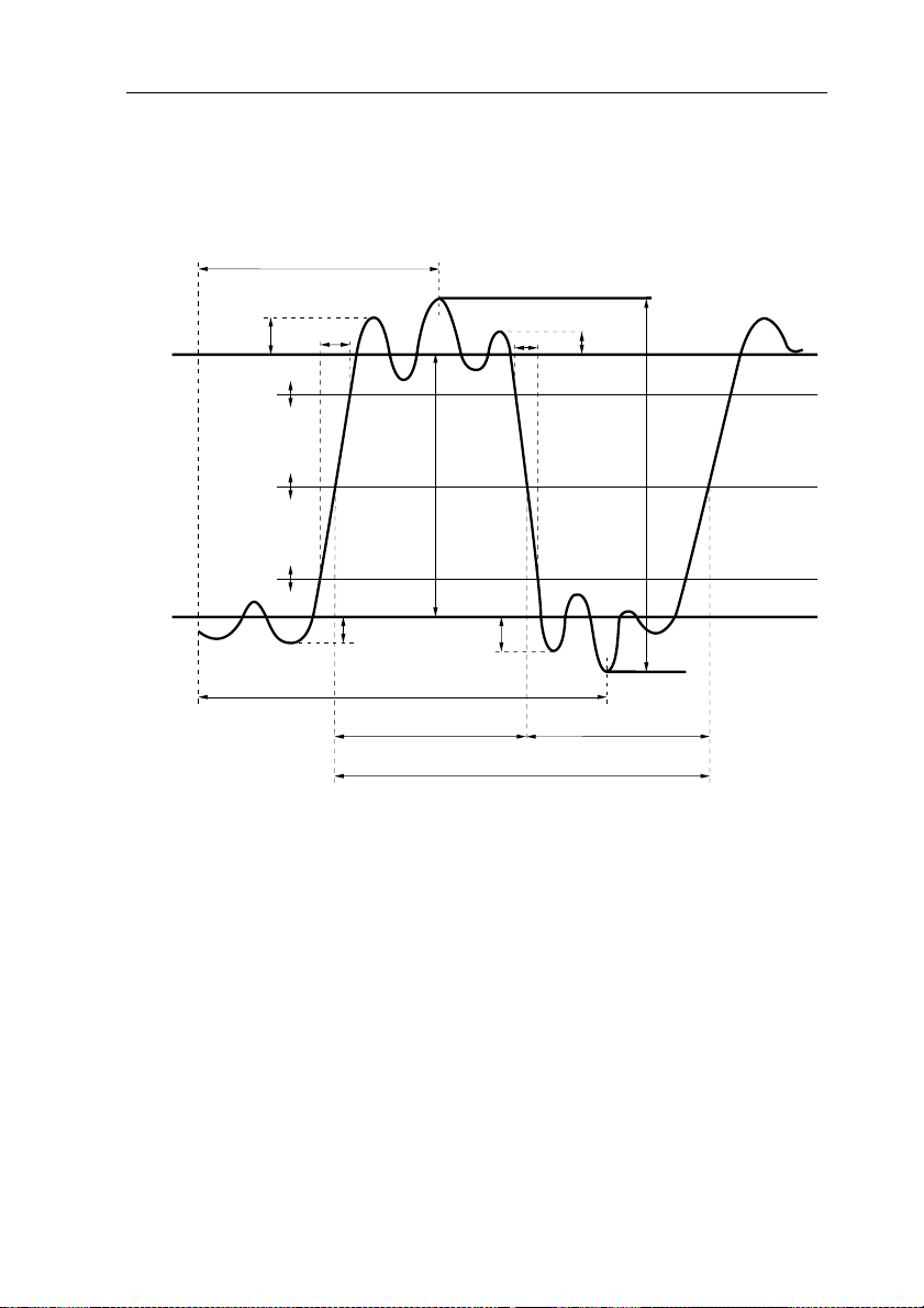
3.3.3 Waveform measurements
The following figure shows the terms used for pulse measurements and the key
words that are used as header nodes in the measurement instructions.
TMAXimum
MAXimum
HIGH
LOW
RISE
OVERshoot
REFerence
HIGH
REFerence
MIDDle
REFerence
LOW
RISE TIME
RISE
PREShoot
TMINimum
AMPLitude
FALL
OVERshoot
FALL TIME
PERiod
FALL
PREShoot
NWIDthPWIDth
PTPeak
MINimum
ST7154
Figure 3.2 Pulse characteristics
The reference high and low parameters determine the desired interval for rise
time and fall time measurements. The default low and high references are 10%
and 90% of the pulse amplitude (= HIGH - LOW).
Default REFerence LOW =LOW + 0.1
Default REFerence HIGH =LOW + 0.9
(HIGH - LOW)
*
(HIGH - LOW)
*
In a similar way, the reference middle parameter determines the desired interval
for pulse width (PWIDth, NWIDth) and duty cycle (PDUTycycle, NDUTycycle)
measurements. When defaulted, the reference middle value is assumed to be at
50% of the amplitude.
Default REFerence MIDDle =LOW + 0.5
(HIGH - LOW)
*
Page 31

3 - 12 USING THE COMBISCOPE INSTRUMENTS
Examples:
MEASure:FALL:TIME? (@3)
Measures the time interval during which the pulse at channel 3 decreases
from 90% to 10% of its amplitude.
MEASure:RISE:TIME? 20,80
Measures the time interval during which the pulse at the default channel 1
increases from 20% to 80% of its amplitude.
The following measure functions and parameters can be programmed:
<measure_function><measure_parameters>
:AC
:AMPLitude
[:DC]
:FALL
:OVERshoot
:PREShoot
:TIME [<reference_low> [,<reference_high> [,<expected_time>
[,<time_resolution>]]]]
:FREQuency [<expected_frequency> [,<frequency_resolution>]]
:HIGH
:LOW
:MAXimum
:MINimum
:NDUTycycle <reference_middle>
:NWIDth <reference_middle>
:PDUTycycle <reference_middle>
:PERiod [<expected_period> [,<period_resolution>]]
:PTPeak
:PWIDth <reference_middle>
:TMAXimum
:TMINimum
:RISE
:OVERshoot
:PREShoot
:TIME [<reference_low> [,<reference_high> [,<expected_time>
[,<time_resolution>]]]]
Notes: - :DCYCle = alias for :PDUTycycle
- :F TIMe = alias for :FALL:TIME
- :RTIMe = alias for :RISE:TIME
Page 32

USING THE COMBISCOPE INSTRUMENTS 3 - 13
3.3.4 Customizing settings
Often, you need more precise control of the measur ements than possible with the
MEASure? query. The combination of CONFigure and READ? is provided to
allow you to program one or more settings that are vital to your application.
Executing this sequence of instructions is equivalent to sending MEASure? For
setting up the instrument, CONFigure uses the same measure functions and
parameters as MEASure?. The CONFigure command does the instrument setup
portion of MEASure?. The READ? query initiates the acquisition, performs the
needed calculations, and returns the desired result.
Since READ? no longer changes instrument settings, commands that are
executed after CONFigure, but before READ?, are taken into effect by the
acquisition. This concept allows you to perform a generic configuration through
CONFigure and then customize the measurement by programming the settings
that are vital to your application. Next the READ? completes the measurement
process.
Example:
CONFigure:AC Configures the instrument to perform an RMS
measurement of the AC component at the default
input channel 1.
SENSe:AVERage ON Sets averaging on.
SENSe:AVERage:COUNT 4 Sets averaging factor at four .
READ:AC? Starts the measurement and returns the averaged
AC-RMS value.
READ? uses the same measure functions and parameters as CONFigure. After
the instrument has been set up for a particular measure function by the
CONFigure command, the same measure function key words can be repeated by
the READ? query header. Moreover, it is allowed to request for another signal
characteristic by specifying a measure function other than that for which the
instrument was configured. However , keep in mind that the instrumen t was set up
by CONFigure for another task. As these settings are not affected by READ?, it
is not guaranteed that the instrument is able to acquire the signal characteristic
that is requested by READ?
Example:
CONFigure:AC Sets up the instrument to perform an RMS
measurement of the AC component.
Page 33

3 - 14 USING THE COMBISCOPE INSTRUMENTS
READ? Requests to execute the default DC measurement.
Since this is not possible with the chosen
configuration, an execution error is generated and
no result is returned.
CONFigure:RISE:TIME Configures the CombiScope instrument to perform a
rise time measurement.
READ:RISE:OVERshoot? Requests to read the rise time overshoot. Because the
CombiScope instrument is able to calculate the rise
overshoot value when it is set up for a rise time
measurement, the desired result is calculated and
returned.
A READ? also allows the same parameter sets as the correspondin g CONFigure
instructions. But, these sets only serve to specify the desired result. They are
ignored as far as they affect instrument settings. The parameters can be sent for
compatibility with the preceding CONFigure command.
Example:
CONFigure:RISE:TIME Configures the oscilloscope to perform a default rise
time measurement (10% to 90% increase of the
signal amplitude).
READ:RISE:TIME? 20,80 Requests for the rise time of the 20 to 80% increase
of the signal amplitude. As the CombiScope
instrument is able to respond to this request, the
desired rise time is calculated and returned.
3.3.5 Multiple measurements
Sometimes it is necessary to perform multiple measurements of the same signal
characteristic. This can be realized by executing multiple MEASure? queries.
However, this implies that the relative time-consuming configuration portion of
MEASure? is unnecessarily repeated. This can be easily avoided by using the
CONFigure and READ? concept as described in the preceding chapter. This
concept allows you to do the configuration only once by sending the CONFigure
command one time. Sending multiple READ? q ueries next, causes the instrument
to repeatedly execute the desired measurement.
Example:
CONFigure:FREQuency Configures the instrument to perform a frequency
measurement.
Page 34

USING THE COMBISCOPE INSTRUMENTS 3 - 15
READ:FREQuency? Starts the acquisition and returns the measured
frequency.
READ:FREQuency? Starts a next acquisition and returns the new
frequency result.
READ:FREQuency? Etc.
3.3.6 Multiple characteristics from a single acquisition.
It is often necessary to determine several signal characteristics from the last
acquired waveform. Starting a new acquisition, as READ? and MEASure? do, is
undesired. For that purpose, READ? is broken down into two additional
instructions, which are the INIT iate[:IMMediate] command and the FETCh ? query .
Executing this sequence of instructions is equivalent to READ?. The
INITiate[:IMMediate] command starts the acquisition. FETCh? determines the
requested signal characteristic and returns the re sult. This concept allows you to
perform several different FETCh? queries on a single set of acquisition data .
Example:
MEASure:AC? Configures the instrument to measure the RMS value
of the AC component of the signal at input channel 1,
starts the acquisition, and returns the desired result.
FETCh:FREQuency? Determines and returns the frequency of the signal
that is acquired by the preceding MEASure? query .
FETCh:RISE:TIME? Uses default parameters to determine and return the
rise time of the first pulse.
As distinct from the READ? query, defaulting the measure function part of the
FETCh? query, causes the CombiScope instrument to return the characteristic
that was requested with the last executed FETCh?, READ? or MEASure? query.
For this reason, the measure function should always be exp licitly specified in the
header of the FETCh? query.
Page 35

3 - 16 USING THE COMBISCOPE INSTRUMENTS
3.3.7 Trigger control via GPIB
You need a separate GPIB command to start a measurement synchronized with
other instruments. This is done by sending the
(Group Execute Trigger) code. The MEASure? and READ? queries do not allow
you to do so, because such a setup causes a query error. With the
INITiate[:IMMediate] and FETCh? concept, it is possib le to meet the requirements
of such applications.
Example:
CONFigure:AC Configures the instrument to measure the AC-RMS
voltage.
TRIGger:SOURce BUS Specifies that the acquisition is to be triggered by
GET or
INITiate Starts the measurement process.
TRG Triggers the acquisition.
*
FETCh:AC? Determines and returns the AC-RMS value.
TRG.
*
TRG command or the GET
*
Page 36

USING THE COMBISCOPE INSTRUMENTS 3 - 17
Configures for channel 2
Switches channel 2 on
Single initiation
Copies CH2-trace to M1_2
Now trace area 2 of memory register 1 is filled with the channel 2 trace.
Fetches AC-RMS of M1_2
Enters AC-RMS value
Prints AC-RMS value
Fetches Peak-To- Peak of M1_2
Enters Peak-To-Peak value
Prints Peak_to_peak value
Fetches amplitude of M1_2
Enters amplitude value
Prints amplitude value
3.3.8 Fetching characteristics from memory traces
The FETCh? query not only allows you to determine a characteristic from the last
acquired waveform, it also allows you to calculate a signal characteristic from a
waveform that is stored in a trace memory element.
Example:
FETCh:RISE:TIME? (@M3_4) Calculates and returns the default rise time
from a waveform that is stored in trace memory
M3_4.
FETCh:PERiod? (@M4_1) Determines and returns the period of the
waveform that is stored in trace memory M4_1.
Notice that such a FETCh? query operates properly only when there is valid
waveform data stored in the trace memory.
PROGRAM EXAMPLE:
In this example the signal acquired via channel 2 is stored in memory register 1.
The AC-RMS, peak-to-peak, and amplitude values of the stored signal are
fetched and printed.
DIM response AS STRING * 10
CALL Send(0, 8, "CONFigure:AC (@2)", 1) ’
CALL Send(0, 8, "SENSe:FUNCtion ’XTIMe:VOLTage2’", 1)’
CALL Send(0, 8, "INITiate", 1) ’
CALL Send(0, 8, "TRACe:COPY M1_2,CH2", 1) ’
’
’
’
CALL Send(0, 8, "FETCh:AC? (@M1_2)", 1) ’
CALL Receive(0, 8, response$, 256) ’
PRINT "AC-RMS value : "; response$ ’
CALL Send(0, 8, "FETCh:PTPeak? (@M1_2)", 1) ’
CALL Receive(0, 8, response$, 256) ’
PRINT "Peak-To-Peak value: "; response$ ’
CALL Send(0, 8, "FETCh:AMPLitude? (@M1_2)", 1) ’
CALL Receive(0, 8, response$, 256) ’
PRINT "Amplitude value : "; response$ ’
Page 37
3 - 18 USING THE COMBISCOPE INSTRUMENTS
3.4 Acquisition
3.4.1 Acquisition control
Several commands exist to control the acquisition process. The following diagram
shows the possible states of the acquisition process, and the way they are
affected by commands.
IDLE state
*RST
ABORt
power on
INIT
or
INIT:CONT ON
Yes
No
Yes
INITiated state
No
INIT:CONT ON
BUS
IMMediate
INTernal
LINE
TRIGger
:SOURce
TRIGger
:LEVel
:SLOPe
Start acquisition
Wait for trigger
Acquisition
Wait for TRIGger state
Wait for complete
Acquisition completed
ST7186
Figure 3.3 The Trigger Model for acquisitions
The trigger model shows that after a
IDLE state. An acquisition doesn’t start until an INITiate command is received.
RST command, the instrument is in the
*
Initiation of the oscilloscope occurs by sending the INITiate[:IMMediate] command
Page 38

USING THE COMBISCOPE INSTRUMENTS 3 - 19
or by setting INITiate:CONTinuous to ON. The INITiate[:IMMediate] command
causes the CombiScope instrument to perform one complete acquisition cycle.
Upon completion of the cycle the instrument returns to the IDLE state.
The INItiate:CONTinuous command is used to select whether the instrument is
continuously initiated or not. When INItiate:CONTinuous is set to ON, the
instrument immediately exits IDLE and starts an acquisition cycle. On completion
of each cycle, the instrument does not return to the IDLE state, but immediately
starts another acquisition cycle.
Before the acquisition takes place, the trigger conditions must be satisfied. These
conditions are programmable to suit the needs of your application, as described in
the next section. After a
So, an INITiate command causes the CombiScope instrument to immediately
trigger the acquisition.
Executing the measurement instructions MEASure? and READ? causes the
acquisition to become initiated automatically . No separate INIT iate commands are
needed. When the FETCh? instruction is used, the instrument must have been
initiated either by a preceding INITiate[:IMMediate] command, or implicitly by a
READ? or MEASure? instruction.
When the CombiScope instrument receives the ABORt command, any
acquisition that is in progress is aborted immediately, and the instrument returns
to the IDLE state. The same occurs when
command distinguishes from
settings, whereas, ABORt does not. For example, when INITiate:CONTinuous is
set to ON, a
the instrument to the IDLE state, but it also sets INITiate:CONTinuous to OFF,
preventing the acquisition to initiate again. Since ABORt does not affect the
instrument settings, an aborted acquisition cycle is immediately initiated again.
RST command not only aborts the pending acquisition and forces
*
RST command, there are no trigger conditions to be met.
*
RST is received. The ABORt
RST in that *RST also resets the instrument
*
*
When the instrument is in the IDLE state, the "no-pending operation" flag that is
associated with the acquisition is set True. The
this flag to signal their "Operation Completed" response. Notice that if
INITiate:CONTinuous is set to ON, the instrument does not return to the IDLE
state when an acquisition cycle has completed. This means that no "Operation
Completed" response is generated after the
OPC and *OPC? commands use
*
OPC and *OPC? commands.
*
Page 39

3 - 20 USING THE COMBISCOPE INSTRUMENTS
3.4.1.1 Triggering
After the measurement is initiated, the CombiScope instrument starts the real
acquisition when the trigger conditions are satisfied, e.g., when the selected
trigger event occurs. The trigger conditions can be ignored during a specific h oldoff time, which can be programmed using the TRIGger:HOLDoff command.
During the hold-off time the event detector is inhibited from acting on any trigger.
Trigger Type
The TRIGger:TYPE command selects the type of triggering, which can be
programmed to EDGE triggering (normal trigger mode) , VIDeo triggering (refer to
section 3.4.1.2 "Video triggering"), LOGic, or GLITch triggering. After a
command, the trigger type is EDGE.
Note: Logic state, pattern, or glitch settings cannot be programmed using SCPI
commands.
Trigger Source
The TRIGger:SOURce command selects the source for the trigger event. The
receipt of the GPIB interface message GET (Group Execute Trigger) or the
common command
trigger source.
TRG serves as the trigger event when BUS is selected as
*
RST
*
The trigger event is determined by the AC line voltage when LINE is selected, and
is derived from the input signal when INTernal is programmed as trigger source.
For the 2-channel CombiScope instruments, EXT e rnal can be programmed as the
trigger source. In that case, channel 4 is selected as external trigger input.
A numeric suffix is used to specify the channel number. For example,
TRIGger:SOURce INT2 selects the signal at input channel 2 to trigger the
acquisition.
When IMMediate is selected, an acquisition d oes not wait for a trigger event. So,
an INITiate command causes the acquisition to begin immediately. After a
command, the trigger source is IMMediate, which means no trigger is required.
Trigger Level
The TRIGger:LEVel command allows you to set the trigger level for all input
channels. Programming the trigger level automatically switches off level peakpeak. The trigger level can be programmed only when the TRIGger:SOURce is
INTernal. The TRIGger:LEVel:AUTO command allows you to switch level peakpeak on or off. Switching on level peak-peak, deactivates the trigger level. After a
RST command the TRIGger:LEVel is set to its maximum value and level peak-
*
peak is switched off.
RST
*
Page 40

USING THE COMBISCOPE INSTRUMENTS 3 - 21
Configures channel 2
Sets channel 2 ON
Trigger source = channel 2
Trigger level = 0.2 V
'The TRIGger:LEVel command also switches level peak-peak off.
Trigger slope = negative
Single initiation
Queries for peak-to-peak
Enters peak-to-peak
Prints peak-to-peak
Trigger Slope
The TRIGger:SLOPe command allows you to define the trigger ed ge for all input
channels, which can be POSitive, NEGative, or EITHer. After a
the TRIGger:SLOPe is set to POSitive.
RST command
*
PROGRAM EXAMPLE:
CALL Send(0, 8, "CONFigure:PTPeak (@2)", 1) ’
CALL Send(0, 8, "SENSe:FUNCtion 'XTIMe:VOLTage2'", 1)’
CALL Send(0, 8, "TRIGger:SOURce INTernal2", 1) ’
CALL Send(0, 8, "TRIGger:LEVel 0.2", 1) ’
CALL Send(0, 8, "TRIGger:SLOPe NEGative", 1) ’
CALL Send(0, 8, "INITiate", 1) ’
CALL Send(0, 8, "FETCh:PTPeak? (@2)", 1) ’
response$ = " "
CALL Receive(0, 8, response$, 256) ’
PRINT "Measured peak-to-peak = "; response$ ’
Trigger Coupling
The TRIGger:LPASs and TRIGger:HPASs commands allow you to select the
Main Time Base (MTB) trigger coup ling by pro gramming a fixed cutoff frequency.
The possible trigger coupling options
reject
High Frequency reject
, and
AC coupling, DC coupling, Low Frequency
are mutually exclusive. The TRIGger:LPASs
and TRIGger:HPASs commands are also mutually exclusive. So, activating the
Low-Pass filter will switch off the High-Pass filter, and vice versa. After a
command, the cutoff frequency is 10 Hertz, which selects trigger coupling AC.
RST
*
Note: When the trigger source is INTernal<n>, signal coupling for one input
channel (n) can be programmed to AC, DC, or GROund using the
INPut<n>:COUPling command.
Page 41

3 - 22 USING THE COMBISCOPE INSTRUMENTS
Sets CH2 on.
Sets CH2 input signal DC coupled.
Sets trigger source = CH2.
Sets Low-Pass filter on + cutoff frequency = 0 Hz;
this selects MTB trigger DC coupling.
Sets CH3 on.
Sets CH3 input signal AC coupled.
Sets trigger source = CH3.
Sets Low-Pass filter on + cutoff frequency = 0 Hz;
this selects MTB trigger DC coupling.
Sets cutoff frequency = 10 Hz; this selects
MTB trigger AC coupling.
DC COUPLING (0 Hz cutoff frequency):
DC coupling causes the signal to be passed over
0dB
DC COUPLING-3dB
FULL BANDWIDTHDC
FREQ.
the full bandwidth (from 0 Hz to 60/100/200 MHz).
T7427
Figure 3.4 DC Coupling
PROGRAM EXAMPLE:
***
*** Select DC coupling on input signal channel 2.
SENSe:FUNCtion:ON "XTIMe:VOLTage2"
INPut2:COUPling DC
TRIGger:SOURce INTernal2
***
*** Select DC coupling on MTB triggering.
TRIGger:FILTer:LPASs:STATe ON
AC COUPLING (10 Hz cutoff frequency):
AC coupling causes the signal to be passed from
0dB
AC COUPLING-3dB
10 Hz to the full bandwidth frequency
(60/100/200 MHz).
FULL BANDWIDTH10Hz
FREQ.
Figure 3.5 AC Coupling
PROGRAM EXAMPLE:
***
*** Select AC coupling on input signal channel 3.
SENSe:FUNCtion:ON "XTIMe:VOLTage3"
INPut3:COUPling AC
TRIGger:SOURce INTernal3
***
*** Select AC coupling on MTB triggering.
TRIGger:FILTer:LPASs:STATe ON
TRIGger:FILTer:LPASs:FREQuency 10
ST7426
Page 42

USING THE COMBISCOPE INSTRUMENTS 3 - 23
Sets Low-Pass filter on + cutoff frequency = 0 Hz
(DC coupling).
Sets cutoff frequency = 30 KHz;
this selects MTB trigger LF-reject.
Sets High-Pass filter on;
this selects MTB trigger HF-reject.
LF-REJECT (30 KHz cutoff frequency):
LF reject (HF passed) causes the signal to be
passed from the cutoff frequency (30 KHz) to the
full bandwidth frequency (60/100/200 MHz).
-3dB
0dB
LF -REJECT
FULL BANDWIDTH30kHz
FREQ.
ST7428
Figure 3.6 LF Reject
PROGRAM EXAMPLE:
TRIGger:FILTer:LPASs:STATe ON
TRIGger:FILTer:LPASs:FREQuency 3E+4
HF-REJECT (30 KHz cutoff frequency)
HF reject (LF passed) causes the signal to be
passed from 0 Hz to the cutoff frequency
(30 KHz).
-3dB
0dB
HF-REJECT
FULL BANDWIDTH30kHz
FREQ.
ST7429
Figure 3.7 HF Reject
PROGRAM EXAMPLE:
***
*** Select HF-reject on MTB triggering.
TRIGger:FILTer:HPASs:STATe ON
3.4.1.2 Video triggering
TV video triggering enables stable triggering on video frames and lines from
various TV standards without adjusting the trigger level, and can be selected by
programming TRIGger:TYPE VIDeo.
Video triggering can be programmed o n signals wi th a positive or negative si gnal
polarity using the TRIGger:VIDeo:SSIGnal command.
Page 43

3 - 24 USING THE COMBISCOPE INSTRUMENTS
The video trigger mode can be programmed to field1, field2, or lines using the
TRIGger:VIDeo:FIELd... commands. The video trigger line can be programmed
using the TRIGger:VIDeo:LINE command.
The video system can be selected using the TRIGger:VIDeo:FORMat:...
commands. The following standard video systems are supported:
- NTSC : 525 lines per frame
- PAL : 625 lines per frame
- SECAM : 625 lines per frame
- HDTV : 1050/1125/1 250 lines per frame
1) Select video triggering and video standard.
Examples: TRIGger:TYPE VIDeo
Selects
TRIGger:VIDeo:FORMat:TYPE SECAM
Selects the
TRIGger:VIDeo:FORMat:LPFRame 1125
Selects the
2) Select video "lines" triggering and program the line to trigger on.
Examples: TRIGger:VIDeo:FIELd:SELect ALL
Selects the video
TRIGger:VIDeo:LINE 512
Selects video line number
TV video
triggering.
SECAM
HDTV
standard with
lines
standard with 625 lines per frame.
1125
lines per frame.
trigger mode.
512
.
3) Select video "field1/2" triggering and program the line to trigger on.
Examples: TRIGger:VIDeo:FIELd:SELect NUMBer
field
Selects video
TRIGger:VIDeo:FIELd:NUMBer 2
Selects the video
TRIGger:VIDeo:FORMat:TYPE PAL
Selects the
TRIGger:VIDeo:LINE 123
Selects video line number
automatically switched to
TRIGger:VIDeo:LINE 325
Selects video line number
automatically switched to
TRIGger:VIDeo:FIELd:NUMBer 1
Selects the video
line number is automatically switched to
triggering.
field2
trigger mode.
PAL
standard with 625 lines per frame.
123
. As a result the video mode is
field1
(field1 = lines 1 .. 312).
325
. As a result the video mode is
field2
(field2 = lines 313 .. 625).
field1
trigger mode. As a result the video
13
(= 325 - 625/2).
Page 44

USING THE COMBISCOPE INSTRUMENTS 3 - 25
3.4.1.3 The trigger modes
A combination of the INITiate:CONTinuous and TRIGger:SOURce command
allows you to define the following trigger modes:
Trigger mode:
>>>Single-shot<<<
Generates one sweep, regardless of any
trigger settings (valid after
>>>Single-shot<<<
Generates one sweep, triggered using
trigger settings.
>>> Single-shot <<<
Generates one sweep, externally triggered
via channel 4 (only for PM33x0B).
>>>Auto trig<<<
Generates continuous sweeps,
independent of any trigger settings.
>>>Normal trig<<<
Generates continuous sweeps, triggered
using trigger settings.
>>> Normal trig <<<
Generates continuous sweeps, externally
triggered via channel 4 (only for PM33x0B).
>>>Single-Shot<<<
Generates one sweep triggered by
or GET, regardless of any trigger settings.
RST).
*
TRG
*
Table 3.1 The TRIGger modes
INITiate
:CONTinuous
OFF IMMediate
OFF
OFF EXTernal
ON IMMediate
ON
ON EXTernal
ON
or
OFF
TRIGger
:SOURce
INTernal<n>
or
LINE
INTernal<n>
or
LINE
BUS
Page 45

3 - 26 USING THE COMBISCOPE INSTRUMENTS
OPERATION STATUS BITS:
STATE DESCRIPTION:
bit 5
Wait for TRIG
bit 3
SWEeping
OPC
idle state (after
RST)000Wait for trigger state (INIT received)
Wait for complete (triggered)
110000= armed
or busy
Finished with acquisition
001
= ready
OPERATION STATUS BITS:
STATE DESCRIPTION:
bit 5
Wait for TRIG
bit 3
SWEeping
OPC
idle state (after
RST)000Wait for trigger state (INIT received)
1 00
= armed
Wait for complete (triggered)
010
= busy
Finished with acquisition
001
= ready
Only in the single-shot and multiple-shot trigger mode (INITiate:CONTinuous
OFF), the bits 3 (SWEeping) and 5 (W aiting for TRIGger) in the OPERation status
are valid. Also the Operation Complete bit (OPC bit 0) in the standard Event
Status Register (ESR) is valid. This allows you to detect whether the instrument
is armed (initiated), triggered (busy with acquisition), or finished with the last
acquisition, i.e., ready for the next acquisition.
SINGLE-SHOT MODE (TB MODE - single):
Commands: CONFigure:AC Configures instrument and sets
single-shot mode.
*
MULTIPLE-SHOT MODE (TB MODE - multi):
*
The bits 3 (SWEeping) and 5 (Waiting for TRIGger) also reflect the acquisition
status, when the "SINGLE ARM'D" button on the front panel was pressed.
Commands: SYSTem:KEY 101 Performs AutoSet.
DISPlay:MENU TBMode Displays TBMODE menu.
SYSTem:KEY 1 Sets INIT:CONT OFF and sets
multiple-shot mode.
Page 46

USING THE COMBISCOPE INSTRUMENTS 3 - 27
1 ms post-trigger
1 ms pre-trigger
3.4.1.4 Pre- and post-triggering
When pre-triggering is selected, the real trace acquisition begins before the
moment that the trigger occurs. Triggering occurs when the trigge r conditions are
satisfied and the instrument leaves the "Wait for TRIGger" state as shown in the
trigger diagram of figure 3.3. In a similar way, post-triggering causes the
acquisition to begin after the moment that the trigger occurs.
trigger moment
SENSe:SWEep:OFFSet:TIME
pre trigger
trigger moment
SENSe:SWEep:OFFSet:TIME
post trigger
begin
Trace
total acquisition time
SENSe:SWEep:TIME
Trace
begin
total acquisition time
SENSe:SWEep:TIME
Figure 3.8 Pre-triggering
time axis
end
ST7191
time axis
end
ST7190
Figure 3.9 Post-triggering
Pre- and post-triggering are programmed wi th the SENSe:SW Ee p:OFFSet:TIME
command. A positive parameter value specifies a post-trigger delay, whereas, a
negative value results in a pre-trigger view.
After
RST, the SENSe:SWEep:OFFSet:TIME is set to -0.005, which results in a
*
pre-trigger view of 5 ms. Because the
(SENSe:SWEep:TIME) is 10 ms, the trigger point is positioned in the middle of
RST value of the total acquisition time
*
the trace.
PROGRAM EXAMPLE:
CALL Send(0, 8, "SENSe:SWEep:OFFSet:TIME 0.001", 1) ’
CALL Send(0, 8, "SENSe:SWEep:OFFSet:TIME -1E-3", 1) ’
Page 47

3 - 28 USING THE COMBISCOPE INSTRUMENTS
3.4.1.5 External triggering
External triggering is only possible for the PM33x0B CombiScope instruments.
Channel 4 is used as the external trigger channel with the following view
possibilities:
- attenuato r positions 0.1 and 1 V/div (AMP key).
- trigger slope positive or negative (EXT TRIG key).
- trigger coupling AC or DC (AC/DC key).
The view facility of the external trigger channel is switched on by sending the
SENSe:FUNCtion:ON "XTIMe:VOLTage4" command, or by sending the
SYSTem:KEY 812 command to simulate the pressing of the TRIG VIEW key on
the front panel.
Note: The view facility of the external trigger channel can only be switched on
when:
• EXTernal or INTernal4 (CH4) is programmed as the trigger source.
• Peak detection is off.
Autoset scans for the presence of a signal on channel 1, 2, and the external
trigger input. If there is a signal present on the external trigger input, the EXTernal
trigger channel is selected as trigger source, and the external trigger view facility
becomes active.
Limitation: The amplitude of the external trigger signal must be high enough for
the sensitivity of the external trigger input (0.1 or 1 V/div.).
Page 48

USING THE COMBISCOPE INSTRUMENTS 3 - 29
3.4.2 Reading trace acquisitions
Once acquisitions are completed, the resulting traces ares placed in TRACe
memory, as shown in the following figure.
TRACe
memory
CH 1
CH 2
CH 3
CH 4
ST7160
@2
@3
@4
@1
INPut
INPut[1]
INPut2
INPut3
INPut4
SENSe
:VOLTage[1]
:VOLTage2
:SWEep
:VOLTage3
:VOLTage4
Main Time Base
Figure 3.10 The trace acquisition flow
The last acquired trace at input channel 1 is placed in the TRACe memory
element named CH1. The trace acquired at channel 2 in CH2, etc. This trace data
can be read by using the TRACe[:DATA]? query.
Example:
TRACe? CH2 Returns the trace that was last acquired at input channel 2.
When new acquisitions are executed, the previously stored traces are not
automatically saved, but overwritten by the new result. When these traces need
to be saved, they have to be copied into other TRACe memory elements, before
a new acquisition is initiated. Refer to section 3.10.2 "Copying traces to memo ry"
for a description about how to copy traces.
As response to the TRACe? query the data is returned as block data.
Section 3.4.3 "Conversion of trace data" specifies the coding of this data and
describes how to convert this data into voltage values.
Page 49

3 - 30 USING THE COMBISCOPE INSTRUMENTS
Dimensions trace buffer
Resets the instrument
Trigger source becomes IMMediate
Number of trace samples becomes 512
Number of trace sample bits becomes 16
Configures for optimal AC-RMS settings
Initiates single acquisition
Requests for channel 1 trace data
Notice the
WAI; before TRACe?. The
WAI command takes care that the
TRACe? CH1 command is executed when the INITiate command is finished.
Reads the channel 1 trace data
Dimensions trace buffer
Resets the instrument
Trigger source becomes IMMediate
Number of trace samples becomes 512
Number of trace sample bits becomes 16
Configures for optimal AC-RMS settings.
Trigger source = GPIB
Opens file TRACE10
10 sequential trace acquisitions
Initiates an acquisition
Triggers via the GPIB
Requests for channel 1 trace
Notice the
WAI; before TRACe?. The
WAI command takes care that
the TRACe? CH1 command is executed when the INITiate command is finished.
Reads the channel 1 trace
Writes the trace buffer to file
Next trace acquisition
Closes file TRACE10
3.4.2.1 Single-shot acquisition
PROGRAM EXAMPLE:
In this example a single-shot trace acquisition is done via channel 1. The trace
bytes are entered as characters in the string response$.
DIM response AS STRING * 1033 ’
CALL Send(0, 8, "*RST", 1) ’
CALL Send(0, 8, "CONFigure:AC", 1) ’
CALL Send(0, 8, "INITiate", 1) ’
CALL Send(0, 8, "*WAI;TRACe? CH1", 1) ’
’
’
’
’
CALL Receive(0, 8, response$, 256) ’
*
*
’
’
’
3.4.2.2 R ep e titive acquisitions
PROGRAM EXAMPLE:
In this example 10 trace acquisitions are done via channel 1. The trace bytes are
entered as characters in the string response$. The 10 trace buffers are written to
the file TRACE10 on the hard disk. Tr iggering is done via the GPIB by sendi ng the
TRG command.
*
DIM response AS STRING * 1033 ’
CALL Send(0, 8, "*RST", 1) ’
CALL Send(0, 8, "CONFigure:AC (@1)", 1) ’
CALL Send(0, 8, "TRIGger:SOURce BUS", 1) ’
OPEN "O",#1,"TRACE10" ’
FOR i=1 TO 10 ’
CALL Send(0, 8, "INITiate", 1) ’
CALL Send(0, 8, "*TRG", 1) ’
CALL Send(0, 8, "*WAI;TRACe? CH1", 1) ’
’
’
’
’
CALL Receive(0, 8, response$, 256) ’
PRINT #1, response$ ’
NEXT i ’
CLOSE ’
*
*
’
’
’
Page 50

USING THE COMBISCOPE INSTRUMENTS 3 - 31
3.4.3 Conversion of trace data
The trace data is sent as a block of binary codes. T race samples can be formatted
to consist of 8 bits (1 byte) or 16 bits (2 bytes) codes, which can be selected by
the FORMat command. Refer to section 3.10.1 "Trace formatting" for a further
explanation of this command. After
When samples are formatted as two bytes, the most signifi cant byte (msb) is se nt
RST the samples are sent as 2 byte codes.
*
first, followed by the least significant byte (lsb). The sample values that are sent
in the block, are coded according to the two’s complement notation. The relation
between the screen positions, the values of the trace samples and the decimal
value of the corresponding binary codes, is shown in the figure below.
screen
range
Screen
position (Ps)
top
mid
bottom
Trace sample
value (Ts)
(127)
32767
25600 (100)
1(1)
0(0)
-1 (-1)
-25600
(-100)
-32768
(-128)
Decimal value
of byte code
32767 (127)
25600 (100)
1(1)
0(0)
65535
(255)
39936
(156)
32768
(128)
trace
range
ST7187
Note: Numbers between parenthesis apply to single byte format.
Figure 3.11 Relation between screen position and trace value
The value of the trace points relate to the vertical position of the corresponding
sample on the screen of the CombiScope instrument. As the figu re above shows,
the sample with value 25600 corresponds with the top position of the screen.
Similarly, the samples with values -25600 and 0 correspond to the bottom and
mid-position respectively. This applies to trace samples that are formatted to
consist of 16 bits (2 bytes). The values that apply to the 8 bit (1 byte) format are
placed between parenthesis.
The ADC allows trace acquisitions that are somewhat outside the vertical screen
boundaries. Trace acquisitions use the full dynamic range of the ADC. This results
in a dynamic trace range of 65535 points, whereas the screen range is limited to
51200 points.
Page 51

3 - 32 USING THE COMBISCOPE INSTRUMENTS
Array of 512 integers
Trace response buffer
Resets the instrument
Data format of 8-bits samples
Single shot initiation
Queries for channel 1 trace
Reads the channel 1 trace
IBCNT% = number of read bytes
The contents of the response$ string of this example will be as follows:
# 3 5 1 4 <8> <byte 1> ... <byte 512> <checksum> <10> ’<10> is terminating LF
3.4.3.1 Conversion of 8-bit samples to integer
As an example a conversion of a trace of 512 "8-bit" samples is shown. The
format is as follows:
trace bytes
# 3 5 1 4 <8> <byte 1> . . . <byte 512> <checksum> <NL
trace sample 512
trace sample 1
byte with decimal value 8
number of trace bytes (514)
number of digits of 514
>
PROGRAM EXAMPLE:
In this example a trace acquisition of 1 byte samples is done. Thereafter , the trace
data is read and converted to integer samples in the array "trace", and the nu mber
of trace bytes and trace samples is printed. The conversion from single byte valu e
to integer is done as follows (refer to figure 3.12):
≥ 128 then integer = byte - 256.
If byte
Example: byte = 255 --> integer = 255 - 256 = -1.
DIM trace(512) ’
DIM response AS STRING * 520 ’
CALL Send(0, 8, "*RST", 1) ’
CALL Send(0, 8, "FORMat INTeger,8", 1) ’
CALL Send(0, 8, "INITiate", 1) ’
CALL Send(0, 8, "*WAI;TRACe? CH1", 1) ’
CALL Receive(0, 8, response$, 256) ’
PRINT "Number of read bytes ="; IBCNT% ’
’
’
’
’
nr.of.digits = VAL(MID$(response$, 2, 1))
nr.of.bytes = VAL(MID$(response$, 3, nr.of.digits)) - 2
PRINT "Number of trace bytes ="; nr.of.bytes
sample.length = ASC(MID$(response$, 3 + nr.of.digits, 1))
nr.of.samples = nr.of.bytes / (sample.length / 8)
PRINT "Number of trace samples ="; nr.of.samples
FOR i = 1 TO nr.of.samples
trace(i) = ASC(MID$(response$, i + 3 + nr.of.digits, 1))
IF trace(i) > 127 THEN
trace(i) = trace(i) - 256
END IF
NEXT i
Page 52

USING THE COMBISCOPE INSTRUMENTS 3 - 33
Arra
y of 512 i
ntegers
Trace response buffer
Resets the instrument
Sets 16 bit sample data format
Single shot initiation
Queries for channel 1 trace
Reads the channel 1 trace
IBCNT% = length of trace buffer
The contents of the response$ string of this example will be as follows:
# 4 1 0 2 6 <16> <msb1> <lsb1> ... <msb512> <lsb512> <sum> <10>
Pointer to next sample
Most Significant Byte
Least Significant Byte
3.4.3.2 Conversion of 16-bit samples to integer
As an example a conversion of a trace of 512 "16-bit" samples is shown. The
format is as follows:
trace bytes
# 4 1 0 2 6 <16> <msb 1> <lsb 1> . . . <msb 512> <lsb 512> <checksum> <NL
trace sample 512
trace sample 1
byte with decimal value 16
number of trace bytes (1026)
number of digits of 1026
>
PROGRAM EXAMPLE:
In this example a trace acquisition of 2 byte samples is done. Thereafter , the trace
data is read and converted to integer samples in the array "trace", and the nu mber
of trace bytes samples is printed. The conversion from double byte ( byte1 = msb
and byte2 = lsb) to integer is done as follows (refer to figure 3.12):
If byte1 < 128 then integer = byte1
If byte1
≥ 128 then integer = (byte1 - 256)
Example: byte1 = 255 & byte2 = 32 --> integer = (255 - 256)
DIM trace(512) ’
DIM response AS STRING * 1033 ’
CALL Send(0, 8, "*RST", 1) ’
CALL Send(0, 8, "INITiate", 1) ’
CALL Send(0, 8, "*WAI;TRACe? CH1", 1) ’
CALL Receive(0, 8, response$, 256) ’
PRINT "Number of trace bytes ="; IBCNT% ’
’
’
’
’
nr.of.digits = VAL(MID$(response$, 2, 1))
nr.of.bytes = VAL(MID$(response$, 3, nr.of.digits)) - 2
PRINT "Number of trace bytes ="; nr.of.bytes
sample.length = ASC(MID$(response$, 3 + nr.of.digits, 1))
nr.of.samples = nr.of.bytes / (sample.length / 8)
PRINT "Number of trace samples ="; nr.of.samples
FOR i = 1 TO nr.of.samples
J = 2 * i + 2 + nr.of.digits ’
byte1 = ASC(MID$(response$, J, 1)) ’
byte2 = ASC(MID$(response$, J + 1, 1)) ’
IF byte1 < 128 THEN
trace(i) = byte1 * 256 + byte2
ELSE trace(i) = (byte1 - 256) * 256 + byte2
END IF
NEXT i
256 + byte2.
*
256 + byte2.
*
256 + 32 = - 224.
*
’
Page 53

3 - 34 USING THE COMBISCOPE INSTRUMENTS
3.4.3.3 Conversion to voltage values
Screen positions correspond to voltage values. This relation is shown in the figur e
below, and is determined by the settings that are programmed by the
SENSe:VOLTage:RANGe:PTPeak and SENSe:VOLTage:RANGe:OFFSet
commands.
Screen
position (Ps)
top
100%
mid
0%
Trace sample
value (Ts)
(127)
32767
25600
(100)
(0)
0
PTPeak
0Volt
OFFSet
Amplitude
value (Vs)
-OFFSet+PTPeak/2
-OFFSet
-OFFSet-PTPeak/2
bottom
-100%
-25600 (-100)
-32768 (-128)
ST7188
Figure 3.12 Relation between screen position and amplitude value
The relation between the screen position Ps and the corresponding voltage
amplitude Vs is expressed by the equations:
Vs = (Ps
Vs = (Ps
PTPeak) / 200 - OFFSet (for 8-bit sample traces)
*
PTPeak) / 51200 - OFFSet (for 16-bit sample traces)
*
As explained in section 3.4.3, there is also a relat ion between the screen position
Ps and the value T s of a trace sample. This relation is expr essed by the equations:
Ps = Ts (for 8-bit sample traces)
Ps = (Ts / 25600)
100 = T s / 256 (for 16-bit sample traces)
*
Eliminating Ps from the preceding equations results in a relation that can be used
to calculate the voltage value Vs from a trace sample Ts. This relation is
expressed by the equations:
Vs = (Ts / 200)
Vs = (Ts / 51200)
PTPeak - OFFSet (for 8-bit sample traces)
*
PTPeak - OFFSet (for 16-bit sample traces)
*
Page 54

USING THE COMBISCOPE INSTRUMENTS 3 - 35
Array of sample voltages
Trace data response string
Peak-to-peak response string
Offset response string
Resets the instrument
Configures for optimal AC-RMS settings
Signal-offset also becomes zero
Initiates single acquisition
Requests channel 1 trace
Reads channel 1 trace
Queries ptp
Reads ptp
IBCNT% = length
Queries offset
Reads offset
IBCNT% = length
1-byte samples
2-byte samples
Pointer to next sample
M.S.B.
L.S.B.
PROGRAM EXAMPLE:
In this program example a trace of 512 samples from the actual signal at input
channel 1 is read. The received data block is converted to an array of voltages. After
each sample conversion the voltage value is printed. This program example works
for traces of 512 samples, consisting of 8 bits (1 byte) or 16 bits (2 bytes) samples.
Note: The program is supplied on floppy under file name EXCNVTRC.BAS.
DIM sample(512) ’
DIM response AS STRING * 1033 ’
DIM peaktop AS STRING * 10 ’
DIM offs AS STRING * 10 ’
’
CALL Send(0, 8, "*RST", 1) ’
CALL Send(0, 8, "CONFigure:AC (@1)", 1) ’
CALL Send(0, 8, "INITiate", 1) ’
CALL Send(0, 8, "*WAI;TRACe? CH1", 1) ’
CALL Receive(0, 8, response$, 256) ’
’
nr.of.digits = VAL(MID$(response$, 2, 1))
nr.of.bytes = VAL(MID$(response$, 3, nr.of.digits)) - 2
sample.length = ASC(MID$(response$, 3 + nr.of.digits, 1))
nr.of.samples = nr.of.bytes / (sample.length / 8)
CALL Send(0, 8, "SENSe:VOLTage:RANGe:PTPeak?", 1) ’
CALL Receive(0, 8, peaktop$, 256) ’
ptpeak = VAL(LEFT$(peaktop$, IBCNT%)) ’
CALL Send(0, 8, "SENSe:VOLTage:RANGe:OFFSet?", 1) ’
CALL Receive(0, 8, offs$, 256) ’
offset = VAL(LEFT$(offs$, IBCNT%)) ’
IF sample.length = 1 THEN
FOR i = 1 TO nr.of.samples ’
trace% = ASC(MID$(response$, i + 3 + nr.of.digits, 1))
IF trace% > 127 THEN trace% = trace% - 256
END IF
sample(i) = trace% / 200 * ptpeak - offset
PRINT sample(i);
NEXT i
ELSE
FOR i = 1 TO nr.of.samples ’
J = 2 * i + 2 + nr.of.digits ’
byte1 = ASC(MID$(response$, J, 1)) ’
byte2 = ASC(MID$(response$, J + 1, 1)) ’
IF byte1 < 128 THEN trace% = byte1 * 256 + byte2
ELSE trace% = (byte1 - 256) * 256 + byte2
END IF
sample(i) = trace% / 51200 * ptpeak - offset
PRINT sample(i);
NEXT i
END IF
’
Page 55

3 - 36 USING THE COMBISCOPE INSTRUMENTS
Dimensions trace string
Dimensions amplitude string
Dimensions frequency string
Configures for AC-RMS
Average factor = 4
Averaging is turned on
Initiates the averaging acquisition
Queries for channel 1 trace
Enters channel 1 trace
The trace samples are averaged over 4 sequential trace acquisitions.
Reads the amplitude
Enters the amplitude
Fetches the frequency
Enters the frequency
The amplitude and frequency are averaged over 4 sequential measured values.
3.5 Averaging Acquisition Data
Acquired traces and measured signal characteristics can be averaged over a
number of acquisitions. The preprocessing AVERAGE function of the
CombiScopes instruments can be enabled by using the SENSe:AVERage[STATe]
command. When this function is set to ON, averaging is done according to the
following formula:
AVG
()n⁄
X
=
n
++
.. X
1
∑
n
In the expression, n specifies the number of acquisitions that is averaged. This
parameter can be programmed by using the SENSe:AVERage:COUNt
command. X represents the acquisition result to be averaged.
Example:
→ SENSe:AVERage:COUnt 16 ’ This sets the average count factor at
Send
16, which means 16 sequential
acquisitions are averaged.
→ SENSe:AVERage ON ’ This enables the AVERAGE function.
Send
When SENSe:AVERage is set to ON and an acquisition is initiated, the
CombiScope instrument takes n (SENSe:AVERage:COUNt) successive
acquisitions, as shown in the figure on the next page. When sufficien t acquisitions
are taken, the final averaged result is returned. Intermediate results cannot be
queried.
PROGRAM EXAMPLE:
Acquire the trace of the actual signal on channel 1 and measure the amplitude
and frequency (averaged over 4 acquisitions).
DIM trace AS STRING * 1033 ’
DIM amplitude AS STRING * 10 ’
DIM frequency AS STRING * 10 ’
CALL Send(0, 8, "CONFigure:AC (@1)", 1) ’
CALL Send(0, 8, "SENSe:AVERage:COUNt 4", 1) ’
CALL Send(0, 8, "SENSe:AVERage ON", 1) ’
CALL Send(0, 8, "INITiate", 1) ’
CALL Send(0, 8, "*WAI;TRACe? CH1", 1) ’
CALL Receive(0, 8, trace$, 256) ’
’
CALL Send(0, 8, "READ:AMPLitude?", 1) ’
CALL Receive(0, 8, amplitude$, 256) ’
CALL Send(0, 8, "FETCh:FREQuency?", 1) ’
CALL Receive(0, 8, frequency$, 256) ’
’
Page 56

USING THE COMBISCOPE INSTRUMENTS 3 - 37
The following diagram shows the possible states of the acquisition process when
"averaging" is on, and the way they are affected by commands.
IDLE state
*RST
ABORt
power on
INIT
or
INIT:CONT ON
Yes
No
Yes
INIT:CONT ON
Wait for AVERage state
No
SENSe:AVERage:COUNt
INITiated state
No
Yes
LINE
INTernal
IMMediate
TRIGger
:SOURce
TRIGger
:LEVel
:SLOPe
Wait for completeWait for trigger
1
acquisition
+
averaging
Figure 3.13 The Trigger Model during acquisition averaging
ST7189
Page 57

3 - 38 USING THE COMBISCOPE INSTRUMENTS
Sets CH1+CH2 on
3.6 Channel Selection
Input channels can be switched on or off by using the SENSe:FUNCtion[:ON] or
SENSe:FUNCtion:OFF commands. An input channel is selected by specifying
the parameter "XTIMe:VOLTage<n>", where the numeric suffix <n> specifies the
input channel number. After a
other channels off (including the EXTernal input for PM33x0A).
Addition of two channels can be selected by specifying the "XTIMe:VOL T age:SUM"
parameter as follows:
> Addition of CH1 and CH2: "XTIMe:VOLTage:SUM 1,2"
> Addition of CH3 and CH4: "XTIMe:VOLTage:SUM 3,4"
Note: Enabling of the addition of input channels (e.g. CH3+CH4), automatically
switches channel 3 and channel 4 on. Disabling of the addition of two
channels (e.g. CH3+CH4), automatically switches channel 3 and
channel 4 off, provided at least one channel remains on.
Programming tip:
If CH1+CH2 is on and CH3 and CH4 are off, CH1+CH2 cannot be programmed
off by sending: SENSE:FUNCtion:OFF "XTIME:VOLTage:SUM 1,2"
Instead, send the command:
SENSe:FUNCtion:ON "XTIME:VOLTage2" ’Sets CH2 on
RST command, channel 1 is turned on and the
*
@1
@2
@3
@4
PROGRAM EXAMPLE:
CALL Send(0, 8, "SENSe:FUNCtion 'XTIMe:VOLTage:SUM 1,2'", 1)
CALL Send(0, 8, "SENSe:FUNCtion:ON ’XTIMe:VOLTage2’", 1)’
INPut
INPut[1]
INPut2
INPut3
INPut4
SENSe
:VOLTage[1]
:VOLTage2
:VOLTage3
:VOLTage4
:FUNCtion
:OFF
[:ON]
:OFF
[:ON]
:OFF
[:ON]
:OFF
[:ON]
"XTIMe:VOLTage1"
"XTIMe:VOLTage2"
:SWEep
"XTIMe:VOLTage3"
"XTIMe:VOLTage4"
Main Time Base
Figure 3.14 Input channel control
’Sets CH2 on, CH1+CH2 off, CH1 remains off.
TRACe
memory
CH 1
CH 2
CH 3
CH 4
ST7158
’
Page 58

USING THE COMBISCOPE INSTRUMENTS 3 - 39
Sets channel 1 AC coupled
Sets channel 2 ground coupled
3.7 Signal Conditioning
The INPut subsystem allows you to condition the input signals, such as
AC/DC/GROund coupling, input filtering, and input impedance selection.
In the digital mode, the SENSe:VOLTage<n>:RANGe:AUTO command allows
you to enable autoranging of the attenuation for each of the input channels <n>
separately.
SENSe
:VOLTage[1]
:VOLTage2
:VOLTage3
:VOLTage4
:FUNCtion
:OFF
[:ON]
:OFF
[:ON]
:OFF
[:ON]
:OFF
[:ON]
"XTIMe:VOLTage1"
"XTIMe:VOLTage2"
:SWEep
"XTIMe:VOLTage3"
"XTIMe:VOLTage4"
Main Time Base
ST7159
@2
@3
@4
@1
INPut
INPut[1]
INPut2
INPut3
INPut4
Figure 3.15 Signal conditioning
3.7.1 AC/DC/ground coupling
The INPut<n>:COUPling command allows you to set the vertical input coupl ing at
AC, DC, or GROund for each input channel separately. After a
all input channels are DC coupled.
RST command,
*
PROGRAM EXAMPLE:
CALL Send(0, 8, "INPut:COUPling AC", 1) ’
CALL Send(0, 8, "INPut2:COUPling GROund", 1) ’
Page 59

3 - 40 USING THE COMBISCOPE INSTRUMENTS
Turns the filter on
Requests for the filter frequency
Reads the filter frequency
Prints: Filter freq. = 2.00E+07
Sets channel 4 impedance at 50
Sets INV CH2 off
Sets INV CH4 on
3.7.2 Input filtering
The INPut:FILTer command allows you to turn the common low-pass filter
(bandwidth limiter) on or off for all input channels at the same time. The cutoff
frequency is fixed at 20 MHz. After a
RST command, the filter is turned off.
*
PROGRAM EXAMPLE:
CALL Send(0, 8, "INPut:FILTer ON", 1) ’
CALL Send(0, 8, "INPut:FILTer:FREQuency?", 1) ’
response$ = " "
CALL Receive(0, 8, response$, 256) ’
PRINT "Filter freq. = "; response$ ’
3.7.3 Input impedance
The INPut<n>:IMPedance command allows you to specify the input impedance
low (50
Ω) or high (1 MΩ) for each input channel separately. After a
command, the impedance of each input channel is 1 M
Ω.
RST
*
PROGRAM EXAMPLE:
CALL Send(0, 8, "INPut4:IMPedance 50", 1) ’
Ω
3.7.4 Input polarity
The INPut<n>:POLarity command allows you to set the polarity of the signal on
the input channel 2 and 4. The polarity can be set to NORMal (default) o r INVerte d
(inverted signal).
PROGRAM EXAMPLE:
CALL Send(0, 8, "INPut2:POLarity NORMal", 1) ’
CALL Send(0, 8, "INPut4:POLarity INVerted", 1) ’
3.7.5 Vertical range and offset
The SENSe:VOLTage<n>:RANGe:PTPeak command allows you to specify the
peak-to-peak range of the signal acquisition over all 8 divisions of the display
screen for each input channel separately. From this peak-to-peak value the
vertical sensitivity per division is calculated as follows:
<vertical_sensitivity> = <peak-to-peak> / 8.
After a
complies to a vertical sensitivity of 200 mV.
RST command, the peak-to-peak value is set at 1.6V for channel 1, which
*
Page 60

USING THE COMBISCOPE INSTRUMENTS 3 - 41
This sets the peak-to-peak range at 800 mV.
So, the vertical sensitivity = 800 / 8 = 100 mV.
This sets a positive vertical offset of 100 mV, i.e., 1 division.
Auto triggering
Sets CH2 on
Sets auto attenuation for channel 2 ON and switches to AC signal coupling
Because the programmed PTPeak and OFFSet values directly affect the trace
values, they can be used to calculate the voltage amplitude of the corresponding
trace samples. As explained in section 3.4.3.3 "Co nversion to voltage values", the
voltage amplitude of a trace sample can be calculated from the equations:
Vs = (Ts / 200)
Vs = (Ts / 51200)
PTPeak - OFFSet (for 8-bit sample traces)
*
PTPeak - OFFSet (for 16-bit sample traces)
*
where Ts = the value of the trace sample
and Vs = the corresponding voltage amplitude
The SENSe:VOLTage<n>:RANGe:OFFSet command allows you to specify the
vertical offset for each input channel. After a
for each input channel is zero.
RST command, the vertical offset
*
PROGRAM EXAMPLE:
CALL Send(0,8 "SENSe:VOLTage2:RANGe:PTPeak .8", 1)
’
’
’
CALL Send(0,8 "SENSe:VOLTage2:RANGe:OFFSet .1", 1)
’
3.7.6 Autoranging attenuators
The AUTO RANGE function automatically selects the vertical input sensitivity to
keep the signal amplitude between 2 and 6.4 divisio ns on the screen. Autoranging
attenuators work independently on the following acquisition channels:
> Input channel 1, 2, 3, and 4 for the PM33x4B CombiScope instruments.
> Input channel 1, and 2 for the PM33x2B CombiScope instruments.
Auto attenuation uses a peak-to-peak calculation to determine the maximum and
minimum value of an acquisition, regardless of the input coupling. When auto
attenuation is switched on for an input channel <n>, the input signal is
automatically forced to AC coupling. Still, it is possible to switch to DC coupling
by programming the INPut<n>:COUPling DC command. However, in that case,
the proper operation cannot be guaranteed.
LIMITATION:
Auto attenuation is limited to 50 mV minimum per division. This minimum
value is used as the noise level to prevent auto attenuation from trying to
adjust noise on an open input channel.
PROGRAM EXAMPLE:
CALL Send(0, 8, "INITiate:CONTinuous ON", 1) ’
CALL Send(0, 8, "SENSe:FUNCtion 'XTIMe:VOLTage2'", 1) ’
CALL Send(0, 8, "SENSe:VOLTage2:RANGe:AUTO ON", 1)
’
Page 61

3 - 42 USING THE COMBISCOPE INSTRUMENTS
Acquisition length = 512 samples.
Acquisition lengthd = 8192 samples.
3.8 Time Base Control
In the digital mode, the SENSe:SWEep:TIME:AUTO command allows you to
enable autoranging of the main timebase (MTB).
3.8.1 Number of samples
The TRACe:POINts command allows you to set the number of sample points,
which is the total acquisition length for all traces. The number of samples i s limited
to discrete values; refer to the TRACe:POINts command reference for a detailed
specification of these values. After a *RST command, the number of samples
is 512.
Note: If the number of samples is changed, the contents of all trace memories
is cleared. So, all previously stored traces are lost!
PROGRAM EXAMPLE:
CALL Send(0, 8, "*RST", 1) ’
CALL Send(0, 8, "TRACe:POINts CH1,8192", 1) ’
3.8.2 Time base speed
The SENSe:SWEep:TIME command specifies the time base of a sweep, which is
the time duration of one complete trace acquisition. Because the
SENSe:SWEep:TIME values are limited in the digital mode by permitted MTB
values, only particular values can be specified with this command. Refer to the
SENSe:SWEep:TIME command reference for a detailed specification of these
values.
Together with the number of trace points (TRACe:POINTs), the
SENSe:SWEep:TIME command determines the Main Time Base (MTB). The
MTB is expressed in seconds per division. Since there are 50 points in each
division, the MTB can be calculated from the following equation:
MTB = 50
*
SENSe:SWEep:TIME / (TRACe:POINts -1 )
Page 62

USING THE COMBISCOPE INSTRUMENTS 3 - 43
Requests sweep time
Reads sweep time
Requests number of trace points
Reads number of trace points
Converts string to variable
Converts string to variable
Calculates the MTB
Prints the MTB
Real time mode off
Real time mode on
Sets peak detection on.
PROGRAM EXAMPLE:
CALL Send(0, 8, "SENSe:SWEep:TIME?, 1) ’
CALL Receive(0, 8, STIME$, 256) ’
CALL Send(0, 8, "TRACe:POINts? CH1, 1) ’
CALL Receive(0, 8, TPOINTS$, 256) ’
SWETIM = VAL(STIME$) ’
TRAPOI = VAL(TPOINTS$) ’
MTB = 50 * SWETIM / (TRAPOI-1) ’
PRINT "Main Time Base ="; MTB ’
In a similar way , the time value Ts that is associated with a trace sample point can
be calculated from the following expression:
Ts = <sample_index >
SENSe:SWEep:TIME / (TRACe:POINts - 1)
*
where <sample_index> is the point number of the sample in the trace.
3.8.3 Real time acquisition
Since there is a physical limit to the maximum sample rate of the ADC , traces with
a duration which is less than 200 ns cannot be sampled within one real-time
acquisition. To allow you to go below the 200 ns limit, the CombiScope instrument
uses particular random sampling techniques, where points in the requested tra ce
are collected from a number of successive acquisitions. The result returned is a
reconstruction of the original signal out of several acquisitions, which is not real
time.
When real time acquisition needs to be guaranteed, the command
SENSe:SWEep:REALtime[:STATe] must be set to ON. This disables the random
sampling techniques. The trade-off is that the SENSe:SWEep:TIME range is
limited to 200 ns. After
RST the :REALtime command is set to OFF.
*
The "peak detection" function allows the Analog-to-Digital Converters (ADC) to
operate at their highest speed, even when a lower time base speed is selected.
The result is that maximum and minimum peaks of the signal are detected, even
at lower time base speeds. This is called oversampling. The
SENSe:SWEep:PDETection[:STATe] command allows you to switch peak
detection on or off.
PROGRAM EXAMPLE:
CALL Send(0, 8, "*RST", 1) ’
CALL Send(0, 8, "SENSe:SWEep:REALtime ON", 1) ’
CALL Send(0, 8, "SENSe:SWEep:PDETection ON", 1) ’
Page 63
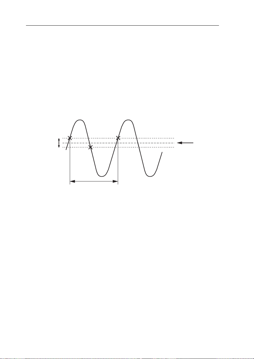
3 - 44 USING THE COMBISCOPE INSTRUMENTS
Auto triggering
Sets CH1 trigger source
Sets auto time base on
3.8.4 Autoranging time base
The AUTO RANGE function of the Main Time Base (MTB) adjusts the time base
automatically, so that two to six waveform periods are displayed on the screen. If
a waveform doesn't contain enough information to calculate its period, the time
base is adjusted to acquire a minimum of two periods. One period of a signal is
determined by three successive crossings of the hysteresis band with the input
signal. The level of the hysteresis band can be set using the TRIGger:LEVel
command.
X3X1
HYSTERESIS
X2
TRIGGER
LEVEL
LIMITATION:
When operating with an acquisition length of 512 points, the maximum input
frequency is 25 MHz. For all other acquisition lengths, the maximum input
frequency is 50 MHz. When the input frequency is greater than the maximum alias
detection frequency, it is no longer possible to detect aliasing.
PROGRAM EXAMPLE:
CALL Send(0, 8, "INITiate:CONTinuous ON", 1) ’
CALL Send(0, 8, "TRIGger:SOURce INTernal1", 1) ’
CALL Send(0, 8, "SENSe:SWEep:TIME:AUTO ON", 1) ’
PERI
D LEN
THPERI
D LEN
TH
Figure 3.16 Definition of a signal period
ST7430
Page 64

USING THE COMBISCOPE INSTRUMENTS 3 - 45
3.9 Post Processing
TRACe
SENSe
CH 1
CH 2
CH 3
CH 4
M1_1
M1_2
M1_3
M1_4
Figure 3.17 Post processing control
3.9.1 How to do post processing
The post processing functions CALCulate1 and CALCulate2 comply with the front
panel functions MATH1 and MATH2 of the CombiScope instrument. They work
only in the digital mode. The use of the CALCulate functions is as follows:
1 Select the source for the post processing function.
2 Specify the settings of the post processing function.
3 Enable the post processing function.
4 Check the result of the post processing function.
M2_1
M2_2
M2_3
M2_4
M3_1
M3_2
M3_3
M3_4
M50_1
M50_2
M50_3
M50_4
CALCulate1
CALCulate2
ST7161
3.9.1.1 Select the source for the post processing function.
Select the trace that is to be sourced into the CALCulate function by sending the
CALCulate<n>:FEED command.
Examples:
→ CALCulate2:FEED "CH3" ’Channel 3 = source for CALC2
Send
Send
→ CALCulate:FEED "M2_1" ’M2_1 = source for CALC1
Empty traces may not be selected as input trace. A memory register 1 location
(M1_ j) may not be specified as the source (feed) for CALCulate1 and a memory
register 2 location (M2_ j) may not be the source (feed) for CALCulate2. After a
RST command, CH1 becomes the input trace for both CALculate functions.
*
Note: CH3 and CH4 cannot be selected as source for the PM33x0B
CombiScope instruments.
Page 65

3 - 46 USING THE COMBISCOPE INSTRUMENTS
CALCulate
CALCulate[1]
CALCulate2
ST7162
SENSe
TRACe
CH 1
CH 2
CH 3
CH 4
M1_1
M1_2
M1_3
M1_4
M2_1
M2_2
M2_3
M2_4
M3_1
M3_2
M3_3
M3_4
CALCulate:FEED "M3_2"
CALCulate2:FEED "M2_4"
M50_1
M50_2
M50_3
M50_4
Figure 3.18 Post processing feed definition
3.9.1.2 Specify the settings of the post processing function.
When desired, specify the settings of the post processing function to be used. The
following settings can be programmed:
- the filter type of the FFT function RECTanguler | HAMMing | HANNing
- the width of the low-pass filter window 3, 5, 7, .., 39, 41 points
- the width of the differential window 3, 5, 7, .., 127, 129 points
Example:
→CALCulate2:TRANsform:FREQuency:WINDow HAMMing
Send
’Defines the Hamming filter for the FFT process.
3.9.1.3 Enable the post processing function.
Enable the desired post processing function by using the :STATe command of the
calculate function concerned. The following post processing functions are
available:
STANDARD AVAILABLE:
- mathematical calculations :MATH
- frequency filtering :FILTer:FREQuency
- frequency domain transformations (FFT) :TRANsform:FREQuency
OPTIONAL:
- histogram transformation :TRANsform:HISTogram
- integratin g tr ace s :INTegra l
- differentiating traces :DERivative (alias :DIFFerential)
Example:
→ CALCulate2:TRANsform:FREQuency:STATe ON ’Enables FFT
Send
The post processing is automatically executed when a trace that is fed into the
CALCulate function is changed. If a mathematical function is switched on, the
other functions are automatically switched off.
Page 66

USING THE COMBISCOPE INSTRUMENTS 3 - 47
Dimensions trace buffer
Channel 3 = source CALC2
Enables FFT-Hamming
Requests for M2_1 trace
Reads the M2_1 trace
3.9.1.4 Check the result of the post processing function.
The results of the post processing functions :MATH
:TRANsform:FREQuency
:TRANsform:HISTogram
are stored in M1_1 for CALCulate1 and in M2_1 for CALCulate2, regardless of
the input (feed) trace.
The results of the post processing functions :FILTer:FREQuency
:INTegral
:DERivative (or :DIFFerential)
are stored in M1_n or M2_n, depending of the input source. When CHn or Mi_n
is the input trace for CALCulate1, the result is placed in M1_n (n = 1, 2, 3, 4).
When CHn or Mi_n is the input trace for CALCulate2, the result is placed in M2_n
(n = 1, 2, 3, 4).
Example:
→ CALCulate2:FEED "CH3"
Send
→ CALCulate2:INTegral:STATe ON
Send
’The result is that the integral of the channel 3 trace is placed in M2_3.
When the result of a calculation is saved in a trace memory location, the other
trace locations of the same memory register are used by the calculate process.
Data stored in these locations may be destroyed. For example, a CALculate1
process that stores the result in M1_2, may also destroy the contents of M1_1,
M1_3, and M1_4. The result of a CALCulate function that is stored in a trace
memory can be read into the controller by using the TRACe? query.
Example:
Send
Read
Note: The result of a CALCulate block can be used as source for the other
PROGRAM EXAMPLE:
DIM response AS STRING * 1033 ’
CALL Send(0, 8, "CALCulate2:FEED ’CH3’", 1) ’
CALL Send(0, 8, "CALCulate2:TRANsform:FREQuency:WINDow HAMMing", 1)
CALL Send(0, 8, "CALCulate2:TRANsform:FREQuency:STATe ON", 1)
CALL Send(0, 8, "TRACe? M2_1", 1) ’
CALL Receive(0, 8, response$, 256) ’
→ TRACe? M2_1 ’Requests for M2_1 trace
← <trace_buffer> ’Reads M2_1 trace
CALCulate block, but not
as source for the same CALCulate block.
’
Page 67

3 - 48 USING THE COMBISCOPE INSTRUMENTS
Channel 1 + channel 2
Math function enabled
The resulting trace (CH1 + CH2) is stored in M1_1.
M1_1 - channel 2
The resulting trace (which is the CH1 trace) is stored in M2_1.
Channel 3 = input source
Channel 3 + channel 2
Math function enabled
The resulting trace (CH3 + CH2) is stored in M1_1.
3.9.2 Mathematical calculations
Mathematical calculations can be performed on 2 traces using the
CALCulate1:MATH and CALCulate2:MATH functions. These functions comply
with the front panel features MA TH1 and MA TH2 respectively. The calculation can
be an addition (+), a subtraction (-), or a multiplication (
resulting trace is automatically set higher than the sum of the attenuations of the
). The attenuation of the
*
individual traces.
PROGRAM EXAMPLE:
CALL Send(0, 8, "CALCulate:MATH (CH1+CH2)", 1) ’
CALL Send(0, 8, "CALCulate:MATH:STATe ON", 1) ’
’
CALL Send(0, 8, "CALCulate2:MATH (M1_1 - CH2)", 1) ’
’
The first argument in the expression that defines the mathematical operation to
be performed, is a trace that may be specified either implicitly, or explicitly by its
trace name. A trace is specified implicitly when the keyword IMPLied is used as
argument in the expression. When IMPlied is specified, the trace that is
programmed with the CALCulate:FEED command is used as the first argument
in the expression. The trace that determines the second argument must always
be specified explicitly by its trace name.
PROGRAM EXAMPLE:
CALL Send(0, 8, "CALCulate:FEED ’CH3’", 1) ’
CALL Send(0, 8, "CALCulate:MATH (IMPLied+CH2)", 1)’
CALL Send(0, 8, "CALCulate:MATH:STATe ON", 1) ’
’
3.9.3 Differentiating and integrating traces
The INTegral function performs a point-to-point integration on a trace. The result
of the integration process is a trace. Each point in the trace is the integral up to
the corresponding point in the original (input) trace.
The DERivative (DIFFerential) function calculates the differential quotient of the
trace points. Each point in the resulting trace is the derivative of the correspon ding
point in the original (input) trace. The width of the differential window can be
programmed from 3 to 129 points in increments of 2 points by the
CALCulate:DERivative:POINts command. After a
points is 5.
RST command, the number of
*
Page 68

USING THE COMBISCOPE INSTRUMENTS 3 - 49
Integral CALC1 on
35 differential points
Differential CALC2 on
Scaling can be adjusted with the "CURSORS TRACK and delta" knobs via the
MATHPLUS - PARAM me nu option.
PROGRAM EXAMPLE:
CALL Send(0, 8, "CALCulate:INTegral:STATe ON", 1) ’
CALL Send(0, 8, "CALCulate2:DERivative:POINts 35", 1)’
CALL Send(0, 8, "CALCulate2:DERivative:STATe ON", 1) ’
3.9.4 Frequency domain transformations
The result of an FFT (Fast Fourier Transformation) calculation is displayed as a
trace of amplitude values (vertically) versus frequency values (horizontally). The
vertical result can be expressed as a relative or an absolute amplitude value. The
CALCulate:TRANsform:FREQuency:TYPE command selects between the
RELative and ABSolute result. The DISPlay:WINDow:TEXT<n>:DATA? query
allows you to read the calculated amplitude and frequency value.
RELATIVE FFT:
A relative FFT calculation consists of a frequency (Hz) and an amplitude in
(dB), relative to the frequency component with the largest amplitude.
ABSOLUTE FFT:
An absolute FFT calculation consists of a frequency (Hz) and an amplitude in
dBm (dB with respect to 1 milliwatt), dBµV (dB with respect to 1 microvolt), or
Vrms (Volt RMS) as selected via the front panel CURSORS - READOUT
softkey menu.
The following FFT window functions can be selected using the
CALCulate:TRANsform:FREQuency:WINDow command:
•
•
The resulting FFT trace is a MIN/MAX (envelope) trace, which means that each
trace point is determined twice (one for the MINimum envelope and one for the
MAXimum envelope). The FFT trace points are scaled between +4 and -4
divisions on the screen. So, the samples values that are returned as response to
a TRACe? query are shifted 4 divisions upwards. The value s of the resultin g FFT
trace points are between -0 dB and -80 dB. This results in the following relation
between screen position and sample value:
The FFT RECTangular function transforms a repetitive time amplitude trace
into its power spectrum.
The FFT HAMMing and HANNing functions reduce the side lobes by applying
a Hamming respectively Hanning window to the input signal. This improves
the visibility of the minor frequency components if the limited area is not
accurately selected.
Page 69

3 - 50 USING THE COMBISCOPE INSTRUMENTS
Trace sample value Trace point
8-bits
top - - - - - 100 25600 - 0 dB
- - - - - - - 75 19200 - 10 dB
- - - - - - - 50 12800 - 20 dB
screen
range
TRACE POINT VALUES:
FFT trace sample values, as entered with the TRACe:DATA? query, can be
converted to FFT point value as follows:
Subtract from the sample value the offset value for 4 divisions:
•
- for 8-bit samples: 4
- for 16-bit samples: 4
Multiply the result with the following correction factor:
•
- for 8-bit samples: -10(dB) / -25 = 0.4
- for 16-bit samples: -10(dB) / -6400 = 0.0015625
- - - - - - - 25 6400 - 30 dB
mid- - - - - 0 0 - 40 dB
- - - - - - - - 25 - 6400 - 50 dB
- - - - - - - - 50 - 12800 - 60 dB
- - - - - - - - 75 - 19200 - 70 dB
bottom - - - 100 - 25600 - 80 dB
Figure 3.19 Relation between screen position and FFT value
25 = 100
*
6400 = 25600
*
16-bits value
trace
range
So, the conversion from a trace sample value (Ts) to a trace point value (Ps) is
expressed by the equations:
- for 8-bit samples: Ps = (Ts - 100)
- for 16-bit samples: Ps = (Ts - 25600)
Note: For an explanation of Ts and Ps, refer to section 3.4.3 "Conversion of
trace data".
When relative FFT calculation is selected, the amplitude trace point values
represent the relative strength of the frequency components. The component with
the highest amplitude is taken as the reference level, referred to as the 0 dB level.
When absolute FFT calculation is selected, the amplitude trace point values depend
on the absolute reference level as selected via the CURSORS - READOUT front
panel menu, which can be one of the following:
- dBm (refere nce = 1 mW) with REFerence IMPedance of 50Ω
- dBm (refere nce = 1 mW) with REFerence IMPedance of 600Ω
-dBµV (reference = 1 µV)
- Vrms (reference = RMS signal amplitude)
0.4
*
0.0015625
*
Page 70

USING THE COMBISCOPE INSTRUMENTS 3 - 51
Absolute FF T amplitudes are calculated fro m the true signal using the information
on the actual attenuator setting in the range from 5 V/div. to 2 mV/div. This results
in an offset value to be added to the relative FFT amplitude for each attenuator
setting. In any attenuator setting, the reference level fo r the absolute FFT value is
calculated from a peak-to- peak amplitude of a sine wave on a screen of 6.34
divisions. This amplitude equals an RMS value of:
6,34 2⁄ 2 2,24≈
This level is used as the reference level (top of screen) for the FFT amplitude
display. For any attenuator setting, the reference level can be calculated as
follows:
2,24 * <number of millivolts per divisions>
Examples: At 20mV/div. : 2.24
At 100mV/div.: 2.24
For a 50Ω system, a signal amplitude of 224 mVrms corresponds to the following
signal power:
P 0,224()
This can also be expressed as a signal level of 0dBm at 50Ω impedance.
The same voltage measured in a 600Ω system corresponds to the following
power level:
P0,224()
This can be calculated as a signal level of:
10 * log
Vrms offset calculation:
A signal of 1 mW at 50Ω impedance is taken as voltag e refere nce at 1 00 mV/div.
From this signal the RMS voltage is calculated as follows:
Urms P *R() 1E-3 *50()0,2236068== =
For a whole screen of 10 divisions, Urms = 2.236068. Depending on the
attenuator setting, the Vrms offset voltage is calculated as follows:
Vrms offset = attenuation
Example for attenuator setting 0.5 V/div.:
2
50⁄ 0,001 W 1 mW≈≈=
2
600⁄ 0,0000836 W 83,6 µW≈≈=
10
83.6E-6 1 mW⁄()10 * log1083.6E-3()10.7 dBm–≈=
20 ≈ 44.8 mVrms
*
100 ≈ 224 mVrms
*
Urms
*
Vrms offset 0,5 *2,236068 1,118034==
Page 71

3 - 52 USING THE COMBISCOPE INSTRUMENTS
dBm - 50Ω offset calculation:
From the Vrms offset value the dBm-50Ω offset value is calculated as follows:
10
dBm 50Ω offset– 20 * Vrms offset 0,2236068⁄()log
=
Note:
P *R() 1E-3 *50()0,2236068==
Example for attenuator setting 0.5 V/div.:
dBm 50Ω offset– 20 * 1,118034 0,2236068⁄()log
10
13,9794==
dBm - 600Ω offset calculation:
From the Vrms offset value the dBm-600Ω offset value is calculated as follows:
10
=
Note:
dBm 600Ω offset– 20 * Vrms offset 0,7745967⁄()log
P *R() 1E-3 *600()0,7745967==
Example for attenuator setting 0.5 V/div.:
dBm 600Ω offset– 20 * 1,118034 0,7745967⁄()log
10
3,1875874==
dBµV offset calculation:
From the Vrms offset value the dBµV offset value is calculated as follows:
10
dBµV offset 20 * Vrms offset 1.0E-6⁄()log
=
Note: 0 dBµ V = 1 µV (1.0E-6 V) at 50Ω impedance.
Example for attenuator setting 0.5 V/div.:
dBµV offset 20 * 1,118034 1E-6⁄()log
10
120,9691==
Page 72

USING THE COMBISCOPE INSTRUMENTS 3 - 53
ATTENUATOR
SETTING:
Vrms:
dBm-50
:
dBm-600
:
dBµV:5V/div2 ,, 1 ,,+11.18034
+
4.4721359
+
2.236068
+
33.9794
+
26.0206
+
20.0+23.187588
+
15.228787
+
9.2081872
+
140.9691
+
133.0103
+
126.9897
0.5
,,
0.2
,,
0.1
,, +1.118034
+
0.4472136
+
0.2236068
+
13.9794
+
6.0206
0.0+3.1875874
-
4.771213
-
10.791813
+
120.9691
+
113.0103
+
106.9897
50
mV/div
20
,, 10 ,,+0.1118034
+
0.0447214
+
0.0223607
-
6.0206
-
13.979392
-
20.0-16.812413
-
24.771206
-
30.791813
+
100.9691
+
93.010308
+
86.989708
5
,,2,,+0.0111803
+
0.0044721
-
26.020632
-
33.97947
-
36.812444
-
44.771282
+
80.96907
+
73.01023
SUMMARY OF CALCULA TED OFFSET VALUES:
Ω
Ω
Note: The PROGRAM EXAMPLE on the next page shows how it is
programmed.
TRACE POINT FREQUENCIES:
The horizontal frequency values (in Hz per point) are calculated from the trace
sample index (point number of the sample in the trace), the acquisition length
(TRACe:POINts), and the MTB (calculated from the SENSe:SWEep:TIME) by the
following equation:
Fs = (<sample_index>
Restriction: Only trace sample data can be queried from trace memories; no
trace administration data, such as acquisition length and MTB value.
This means that these values must be queried from the actual input
channel signal, which is taken as the source for the FFT process. So,
take care that the acquisition length nor the MTB is changed between
activating the post processing function and reading the trace memory
where the post processing trace is stored.
1250) / (TRACe:POINts * MTB * 50)
*
Page 73

3 - 54 USING THE COMBISCOPE INSTRUMENTS
PROGRAM EXAMPLE:
The following program example converts a relative or absolute FFT trace of 512
samples of 1 or 2 bytes from the signal on channel 1 via the MATH1 feature as
follows:
Before running this program, first make the FFT selections desired via the
•
front panel, such as:
> MATH - MATH1 "on" and "fft".
> CURSORS "on" and "m1.1".
> MATH - PARAM - FILTER "hamming", "hanning", or "re c tang".
> MATH - PARAM - READOUT "rel" to select relative FFT.
> MATH - PARAM - READOUT "abs" to select absolute FFT.
+ CURSORS - READOUT "dBm + 50Ω", "dBm + 600Ω", "dBµV", or
"Vrms".
Request the following values:
•
> The acquisition length using the TRACe:POINts? CH1 query.
> The sweep time to calculate the MTB using the SENSe:SWEep:TIME?
query.
MTB = (sweep_time
The calculation factor to determine the sample point frequencies is
determined as follows:
calc = 1250 / (acquisition_length
> The peak-to-peak voltage to calculate the attenuation using the
SENSe:VOLTage:RANGe:PTPeak? query.
Attenuation = peak-to=peak / 8.
> The FFT type, i.e., ABSolute or RELative, using the
CALCulate:TRANsform:FREQuency:TYPE? query.
50) / (acquisition_length - 1).
*
MTB * 50).
*
Read the FFT trace from memory register m1.1 using the TRACe? M1_1
•
query.
Convert and print the frequency and amplitude values of the FFT trace sample
•
points according to the formulas as explained before.
Note: The program prints the calculated values in groups of 20 sample
points on the screen of your computer.
Note: The program is supplied on floppy under file name EXFFTTRC.BAS.
Page 74

USING THE COMBISCOPE INSTRUMENTS 3 - 55
This turns the histogram function on
35 filter points
Filter CALC1 on
3.9.5 Histogram functions
The HIST ogram function calculates an amplitude distribution of the incoming trace.
The number of points in the histogram trace is 512. Each point in the histogram
specifies the number of times that a data point of the incoming trace is within a
particular amplitude belt. Since there are 512 histogram points, there are also 512
amplitude belts. The range of the amplitude belts is determined by the selected
peak-to-peak range (SENSe:VOLTage:RANGe:PTPeak) and is expressed by the
following equation:
amplitude belt = peak-to-peak range / 512
Notice that a histogram contains 512 valid data points. The number of points
(TRACe:POINts) of the trace memory location where the histog ram is stored, may
exceed this value. In that case the values of the trace positions above 512 have
to be ignored.
The histogram is displayed on the screen in the area between +3 and -2 divisions
vertically, and between the third and the seventh division horizontally. The
horizontal axis represents the amplitude in volts. The vertical axis represents the
number of occurrences of an amplitude in percents.
PROGRAM EXAMPLE:
CALL Send(0, 8, "CALCulate:TRANsform:HISTogram:STATe ON", 1)
’
.
3.9.6 Frequency filtering
The FILTer function performs digital low-pass filtering to suppress undesired
frequency noise. The width of the filter window can be programmed from 3 to 41
points in increments of 2 points. After a
PROGRAM EXAMPLE:
CALL Send(0, 8, "CALCulate:FILTer:FREQuency:POINts 35", 1)
CALL Send(0, 8, "CALCulate:FILTer:FREQuency:STATe ON", 1)
RST command, the number of points is 19.
*
’
’
Page 75

3 - 56 USING THE COMBISCOPE INSTRUMENTS
3.10 Trace Memory
The trace memory of the CombiScopes instruments consists of space for channel
acquisition traces (CH1 to CH4) and memory regi ster traces (M1 to M8 and M9 to
M50 extended). The amount of acquisition and register space depends on the
following:
Whether the CombiScope instrument is equipped with standard or with
•
extended memory.
The specified acquisition length (number of trace samples) with the
•
TRACe:POINts command.
Example:
Send → TRACe:POINts CH1,8192
This command specifies an acquisition length of 8192 samples for all traces.
Notes: - Only the following trace acquisition lengths can be programme d:
512, 2024 (2K), 4096 (4K), 8192 ( 8K), 16384 (16K), or 32768 (32K)
- If a different acquisition length is programmed, the contents of all
acquisition and register space is cleared. So, all previously stored
traces are lost!
- After a
- The resulting traces of the post processing functions are always
stored in memory register 1 for CALCulate1 functions and in
memory register 2 for CALCulate2 functions.
RST command, the number of trace samples is 512.
*
TRACe
M50_1
M50_2
M50_3
M50_4
SENSe
CH 1
CH 2
CH 3
CH 4
M1_1
M1_2
M1_3
M1_4
M2_1
M2_2
M2_3
M2_4
M3_1
M3_2
M3_3
M3_4
Note: For standard memory, 8 memory registers are available (M1 to M8).
For extended memory, 50 memory registers are available (M1 to M50).
Figure 3.20 Trace memory control
Note: CH3 and CH4 cannot be selected as the source for the PM33x0B
CombiScope instruments. Instead the external channel can be selected,
e.g., M1_E.
ST7163
Page 76

USING THE COMBISCOPE INSTRUMENTS 3 - 57
Length of trace samples = 16 bits
Length of trace samples = 8 bits
The following table shows the relation between the trace acquisition length
(TRACe:POINts) and the available channel (CHx) and memory traces (Mx).
TRACe:POINts CHANNELS: MEMORY REGISTERS:
STANDARD:
512
2K
4K
8K
(PM33x0B)
4(2+EXT)
4(2+EXT)
2(2)
1(1)
M1 .. M8
M1 .. M2
M1 .. M2
M1 .. M2
EXTENDED:
512
8k
16K
32K
Examples:
- Standard memory 4K acquisition length allows, for example:
CH1 + M1_1 + M2_1 + CH3 + M1_3 + M2_3
- Extended memory 32K acquisition length allows, for example:
CH2 + M1_2 + M2_2
(PM33x0B)
4(2+EXT)
4(2+EXT)
2(2)
1(1)
M1 .. M50
M1 .. M2
M1 .. M2
M1 .. M2
Table 3.2 Relation between acquisition length and available trace memory
Note: Delayed Time Base (DTB) acquisition traces are only saved in th e CH1
to CH4 memory, when the acquisition length is 512 samples. DTB
acquisitions can only be defined via front panel operations.
3.10.1 Trace formatting
The FORMat command allows you to format the resolution of trace sample
values. The resolution is determined by specifying the number of bits used to
code the sample values of all trace acquisitions. Trace samples can be
programmed to be formatted as 16 bits (2 bytes) or as 8 bits (1 byte). After a
command, the number of trace sample bits is 16 (2 bytes). Notice that the
contents of acquisition and register space is not cleared when a different trace
format is programmed.
RST
*
PROGRAM EXAMPLE:
CALL Send(0, 8, "*RST", 1) ’
CALL Send(0, 8, "FORMat INTeger,8", 1) ’
Page 77

3 - 58 USING THE COMBISCOPE INSTRUMENTS
Channel 1 on
Channel 2, 3, 4 off
Channel 3 also on
’ The result is that the acquisition traces of the channels 1 and 3 are copied to M2_1 respectively M2_3
The result is that the previously stored traces in M2_1 and M2_3 are copied to M3_1 respectively m3_3
3.10.2 Copying traces to memory
The TRACe:COPY command allows you to copy the contents of a memory
register to another memory register. This allows you to fill a memory register with
traces from one of the following sources:
Copy an acquisition trace from one of the input channels.
•
Example:
Send → TRACe:COPY M1_2,CH2 ’ Copies from CH2 to M1_2
Note: The result of this command is also that the acquisition traces of other
channels (CHn) are copied into M1_n, provided channel CHn is on.
So, all previously stored traces in M1 are lost!
Copy a previously stored trace from another trace memory register.
•
Example:
Send → TRACe:COPY M2_2,M1_2 ’ Copies from M1_2 to M2_2
Note: The result of this command is also that all stored traces of M2_N are
copied into M1_n, provided a trace was stored before. So, all
previously stored traces in M2 are lost!
PROGRAM EXAMPLE:
CALL Send(0, 8, "*RST", 1) ’
CALL Send(0, 8, "SENSe:FUNCtion ’XTIMe:VOLTage3’", 1) ’
’
CALL Send(0, 8, "TRACe:COPY M2_1,CH1", 1)
CALL Send(0, 8, "TRACe:COPY M3_1,M2_1", 1)
’
.
.
Page 78

USING THE COMBISCOPE INSTRUMENTS 3 - 59
Dimensions trace buffer
Requests for channel 1 trace
Reads the channel 1 trace
IBCNT = number of data bytes
Sends fixed command part without EOI
Sends variable <trace block> without EOI
Sends dummy string with EOI detection
3.10.3 Writing data to trace memory
The TRACe command allows you to write data from the controller into a memory
register. The following possibilities are available:
Write a previously read trace using the TRACe? query.
•
Example:
Send → TRACe? CH3 ’Queries for CH3 trace
Read ← <trace block> ’Reads trace data block
Send → TRACe M2_3,<trace block> ’Writes data block to M2_3
The result is that trace area M2_3 is filled with the acquisition trace of cha nnel 3.
Programming note:
The fixed command part (TRACe M2_3,) and the variable <trace block>
must be sent separately. So, no EOI (End Or Identify) detection in
between. Also the <trace block> must be sent without EOI detection and
detection of the EOL (End Of Line) code, because the <trace block> could
contain the EOL character, e.g., code 10 for CR
Write a trace of identical constants (range = -32767 ... 32767).
•
Example:
Send → TRACe M2_4,1028 ’1028 = 1024 + 4 = 0404 hex.
This command fills all memory register M2_4 locations with the constant 0404
hexadecimal for 16-bit samples, and with 04 hexadecimal for 8-bit samples.
.
Note: A trace can only be written to memory register space (Mi_n) and not
to acquisition space (CHn).
PROGRAM EXAMPLE:
DIM response AS STRING * 2000 ’
CALL Send(0, 8, "TRACe? CH1", 1) ’
CALL Receive(0, 8, response$, 256) ’
length = IBCNT% ’
CALL Send(0, 8, "TRACe M2_3,", 0) ’
CALL Send(0, 8, LEFT$(response$,length), 0)
CALL Send(0, 8, "", 1) ’
’
Page 79

3 - 60 USING THE COMBISCOPE INSTRUMENTS
Dimensions trace buffer 1
Dimensions trace buffer 2
Requests for channel 1 trace
Reads channel 1 trace into trace1$
Input source = CH1
Enables frequency filtering; the filtered channel 1 trace is stored in M1_1
Requests for M1_1 trace
Reads M1_1 trace into trac e2$
3.10.4 Reading data from trace memory
The TRACe? query allows you to read the contents from one of the foll owing trace
memory registers:
An acquisition trace from one of the input channels (CH1 to CH4).
•
Previously stored trace data from one of the memory registers (M1 to M8 or to
•
M50). This can be either an acquisition trace or a trace of constant values
(refer to section 3.10.3).
The result of a post processing function; CALCulate1 in M1 and CALCulate2
•
in M2 (refer to section 3.9 "Post processing").
PROGRAM EXAMPLE:
’
*****
’Read the actual channel 1 trace into trace1$ and the filtered
’channel 1 trace into trace2$.
’
*****
DIM trace1 AS STRING * 2000 ’
DIM trace2 AS STRING * 2000 ’
CALL Send(0, 8, "TRACe? CH1", 1) ’
CALL Receive(0, 8, trace1$, 256) ’
CALL Send(0, 8, "CALCulate:FEED ’CH1’", 1) ’
CALL Send(0, 8, "CALCulate:FILTer:FREQuency:STATe ON", 1)
’
.
CALL Send(0, 8, "TRACe? M1_1", 1) ’
CALL Receive(0, 8, trace2$, 256) ’
Page 80

USING THE COMBISCOPE INSTRUMENTS 3 - 61
Sets brightness at 0.3
3.11 Screen/Display Functions
3.11.1 Brightness control
The DISPlay:BRIGhtness command allows you to control the brightness of the
trace(s) displayed on the screen of your Comb iScope instru men t on a scale from
0.0 (low) to 1.0 (high). After a
PROGRAM EXAMPLE:
CALL Send(0, 8, "DISPlay:BRIGhtness .3", 1) ’
3.11.2 Display functions
The DISPlay:WINDow and DISPlay:MENU commands allow you to use the
following display functions:
The WINDow1 functions use the front panel screen display of MEAS1/MEAS2,
•
CURSORS, and MATH-FFT to read measurement data from the CombiScope
instrument (refer to section 3.11.2.1).
The WINDow2 function to write user-defined text on the screen (refer to
•
section 3.1 1.2.2).
The MENU function to display softkey menus on the screen (refer to
•
section 3.11.2.3).
RST command, the brightness intensity is 0.18.
*
.
The layout of the display areas on the screen is as follows:
WINDow[1]
MENU
WINDow2
Figure 3.21 Screen layout of display functions
Page 81

3 - 62 USING THE COMBISCOPE INSTRUMENTS
3.11.2.1 Readout of measurement data
The DISPlay:WINDow[1]:TEXT<n>:DATA? query allows you to acquire
measured data as displayed on the upper line(s) of the screen of your
CombiScope instrument. The following measured data valu es can be selected by
specifying the number <n> in the query:
NUMBER <n>: MEASUREMENT VALUE:
1, 2
10, 1 1, 12, 13, 20, 21,
30, 40, 51, 52
60, 61
MEAS1/MEAS2 DA TA:
The MEAS1 and MEAS2 functions must be enabled and selected via front panel
control. MEAS1 data is read by sending the DISPlay:WINDow:TEXT1:DATA?
query and MEAS2 data by sending the DISPlay:WINDow:TEXT2:DATA? query,
followed by reading the response strings.
The format of a response string is as follows:
<meas_type>,<meas_value>,<suffix_unit>
DESCRIPTION: <meas_type> <suffix_unit>:
DC voltage
AC-RMS voltage
minimum voltage
maximum voltage
peak-to-peak voltage
low level voltage
high level voltage
overshoot percentage
preshoot percentage
frequency
period time
pulse width
rise time
fall time
duty cycle percentage
delay time between 2 channels
MEAS1, MEAS2 data
CURSORS data
MA TH - FFT frequency, amplitude
dc
rms
min
max
pkpk
low
high
over
pre
freq
T
puls
rise
fall
duty
del
V
V
V
V
V
V
V
%
%
Hz
s
s
s
s
%
s
Page 82

USING THE COMBISCOPE INSTRUMENTS 3 - 63
Example:
Send →
Send → DISPlay:MENU MEASure ’Switches MEASURE menu on
Send → SYSTem:KEY 2;KEY 4 ’Switches MEAS1 and MEAS2 on
Send → DISPlay:WINDow:TEXT1:DATA? ’Requests MEAS1 data
Read ← pkpk,6000E-04,V ’Response = peak-to-peak 0.6 volt.
CURSORS DATA:
The CURSORS function offers a wide variety of voltage and time readouts. The
following readout selections can be made via the CURSORS - READOUT softkey
menu:
<n>: TYPE: UNIT: DESCRIPTION:
10
11
12
13
20
21
30
40
51
52
RST ’Switches MEAS1 & 2 off
*
dV
dY
V1
V2
Vdc
dT
F
dX
phase
T1-trg
T2-trg
V
U
V
V
V
s
Hz
U
*
s
s
Voltage difference (delta-V) between the cursors.
Vertical voltage (X-deflection on).
Absolute voltage of cursor 1 to ground.
Absolute voltage of cursor 2 to ground.
DC voltage
Time difference (delta-T) between the cursors.
Frequency (1/dT) in Hertz.
Horizontal voltage (X-deflection on).
The phase between two channels in degrees Celsius.
stands for degrees ° sign)
(
*
The time between cursor 1 and the trigger event.
The time between cursor 2 and the trigger event.
MATH - FFT DATA:
The MATH1/MATH2 - FFT functions offer the readout of the relative or absolute
frequency and amplitude. The following readout selections can be made via the
CURSORS - READOUT and MATH - FFT - PARAM softkey menus:
<n>: TYPE: UNIT: DESCRIPTION:
6061FFT-freq
FFT-amplHzvariable
FFT frequency in Hertz.
FFT amplitude in:
- Relative FFT selected: dB
- Absolute FFT selected: dBm, dbµV, V (Vrms)
Page 83

3 - 64 USING THE COMBISCOPE INSTRUMENTS
Displays MEASURE menu
Enable MEAS1 & MEAS2 and select MEAS1-DC and MEAS2-frequency
Queries for volt-dc
Reads volt-dc value
Queries for time-freq
Reads time-freq value
PROGRAM EXAMPLE:
Read and print the DC and frequency characteristic of the actual signal usi ng the
MEAS1 and MEAS2 functions. The program stops to let you make the req uested
MEAS selections.
DIM response AS STRING * 30
CALL Send(0, 8, "DISPlay:MENU MEASure", 1) ’
’
’
*****
’
PRINT ">>> Press the LOCAL key, set MEAS1 function on, and select
PRINT ">>> Set MEAS2 function on and select MEAS2-time-freq."
PRINT ">>> Press any key on the controller keyboard when finished."
WHILE INKEY$ = "": WEND
CALL Send(0, 8, "DISPlay:WINDow:TEXT1:DATA?", 1) ’
CALL Receive(0, 8, response$, 256) ’
PRINT "Measured volt-dc = "; LEFT$(response$, IBCNT% - 1)
CALL Send(0, 8, "DISPlay:WINDow:TEXT2:DATA?", 1) ’
CALL Receive(0, 8, response$, 256) ’
PRINT "Measured time-freq = "; LEFT$(response$, IBCNT% - 1)
.
MEAS1-volt-dc."
Page 84

USING THE COMBISCOPE INSTRUMENTS 3 - 65
Enables display of text
Displays the text: Remote control on the screen of your CombiScope instrument
Clears the text
Displays: 1.25 k
Displays:
Displays: CH1
Displays the text: 1.25 kW CH1 on the screen of your CombiScope instrument
Selects and displays the
CURSORS menu
Switches the CURSORS menu
display off
3.11.2.2 Display of user-defined text
The DISPlay:WINDow2:TEXT commands allow you to define and clear the user
text on the screen area of your CombiScope instrument. After a
the display of the previously defined user text is turned off.
RST command,
*
PROGRAM EXAMPLE 1: (text as string data)
CALL Send(0, 8, "DISPlay:WINDow2:TEXT:STATe ON", 1) ’
CALL Send(0, 8, "DISPlay:WINDow2:TEXT:DATA ’Remote control’", 1)
’
’
.
PROGRAM EXAMPLE 2: (text as block data)
CALL Send(0, 8, "DISPlay:WINDow2:TEXT:CLEar", 1) ’
CALL Send(0, 8, "DISPlay:WINDow2:TEXT:DATA #01.25 k", 0)’
CALL Send(0, 8, CHR$(25), 0) ’
CALL Send(0, 8, " CH1", 1) ’
’
’
.
Ω
Note: The ASCII character 25 (= ↓ ) is displayed as Ω on the screen of your
CombiScope instrument.
3.11.2.3 Selection of softkey menus
The DISPlay:MENU commands allow you to select and enable the display of a
softkey menu. If a menu is selected via the DISPlay:MENU command, the display
is automatically enabled. After a
turned off.
RST command, the display of softkey menus is
*
PROGRAM EXAMPLE:
CALL Send(0, 8, "DISPlay:MENU CURSors", 1) ’
CALL Send(0, 8, "DISPlay:MENU:STATe OFF", 1) ’
.
.
Page 85

3 - 66 USING THE COMBISCOPE INSTRUMENTS
3.12 Print/Plot Functions
The HCOPy:DEVice <TYPE> command allows you to select a hardcopy device.
The following selections can be made:
DEVICE: TYPE: NOTE:
Plotter
Plotter
Plotter
Plotter
Plotter
Plotter
Plotter
Printer
Printer
Printer
Printer
Printer
Generator
The HCOPy:DATA? query allows you to request a hardcopy of the picture on the
screen of your CombiScope instrument. The response data is formatted
according to the current printer/plotter options, which can be selected via the front
panel UTILITY menu. After a
selected.
HPGL
HP7440
HP7550
HP7475A
HP7470A
PM8277
PM8278
FX80
HP2225
LQ1500
HPLASER
HP540
DUMP_M1
HPGL plot data format
Epson FX80 compatibles (9 points)
ThinkJet
Epson LQ150 compatibles (24 points)
HP LaserJet series II & III
HP DeskJet (new style protocol)
Trace dump to one of the arbitrary waveform
generators PM5138, PM5139, or PM5150.
RST command, the option "plotter; HPGL" is
*
The response data to a HCOPy:DATA? query can be sent to a connected plotter
or printer to make a hardcopy. The response data is sent as block data of
indefinite length and is therefore, preceded by the preamble #0 of 2 bytes. This
preamble must be removed from the beginning of the block data, before sending
it to a plotter or printer device.
Page 86

USING THE COMBISCOPE INSTRUMENTS 3 - 67
Dimensions address array
Dimensions response string
Timeout at 10 seconds
Selects the PM8277 plotter
Requests for hardcopy data
Reads the hardcopy data
IBCNT = number of read bytes
The first 2 characters of the response block data are #0 (preamble for indefinite length)
They must not be sent to the plotter; so, send characters 3 until 3+length-2.
No End detection
End of data block
read
DSO
response
data
1)
send
HCOPy:DATA?
send
plot/print
data
3)
2)
data
buffer
CONTROLLER
PLOTTER
PRINTER
1) Send the query
HCOPy:DATA? via the GPIB.
2) Read the block response
data via the GPIB.
3) Send the print/plot data part
to the printer/plotter.
ST7219
Figure 3.22 Hardcopy of screen on printer/plotter
PROGRAM EXAMPLE:
Select one of the supported GPIB plotters, set its address at 22 and connect the
plotter via IEEE to the controller. Create a screen picture on the DSO that you
want to plot and run the following program.
DIM addr(2) ’
DIM response AS STRING * 15000 ’
CALL IBTMO(0, 13) ’
CALL Send(0, 8, "HCOPy:DEVice PM8277", 1) ’
CALL Send(0, 8, "HCOPY:DATA?", 1) ’
CALL Receive(0, 8, response$, 256) ’
length = IBCNT% ’
PRINT "Number of hardcopy bytes ="; length
’
*****
’
’
’
*****
CALL Send(0, 22, MID$(response$, 3, length - 2), 0) ’
CALL Send(0, 22, "", 1) ’
.
.
.
.
.
.
Page 87

3 - 68 USING THE COMBISCOPE INSTRUMENTS
Sets the time to 25 minutes and 36
seconds past 2 o'clock in the
afternoon.
Sets the date to 15 december 1993.
3.13 Real-Time Clock
The real-time clock keeps track of the current date and time. The date and time
are stamped on acquired waveforms to be sent to a computer or to be output to
a hardcopy device. The time of stamping is also the time of th e acquisition trigger .
The SYST em:TIME comman d sets the time in hours, minutes, and seconds. On ly
a 24-hours time format is supported. The format of the displayed time cannot be
selected.
The SYSTem:DATE command sets the date in years, months, and days.
PROGRAM EXAMPLE:
CALL Send(0, 8, "SYSTem:TIME 14,25,36", 1)
CALL Send(0, 8, "SYSTem:DATE 1993,12,15", 1)
3.14 Auto Calibration
Calibration is only possible when the CombiScope instrument is warmed up. The
instrument data is calibrated automatically by sending the
CALibration? query. The internal calibration lasts several minutes. A "0" result is
returned after correct calibration, and a "1" result is returned when the calib ration
failed. Notice that the response to the calibration que ry i s on ly return ed whe n the
calibration has completed.
CAL? or the
*
During the calibration process bit 0 "Calibrating" is set in the operation status
condition register. This bit cannot be read during the execution of the
CALibration? query, because these queries are sequential commands. This bit
can be read after sending the CALibration command, which is an overlapped
command. The completion of the CALibration command is reported in the
standard Event Status Register (ESR) bit 0 (OPC bit set to 1). When the
calibration is finished, bit 8 in the QUEStionable status reports a possible
calibration error (if set to 1).
Note: Execute calibration only when it is needed, e.g., when a message on the
screen of your CombiScope instrument requests to do so.
CAL? or
*
Page 88

USING THE COMBISCOPE INSTRUMENTS 3 - 69
Starts the calibration
Disables the time out mechanism
Waits for the calibration to finish and reads the result
Sets time out back to 10 seconds
0 = okay
1 = wrong
Defines "ServReq" routine call after SRQ
Enables SRQ mechanism
Sets bit 0 (Calibration) true in the case of negative transition (from 1 to 0).
Enables bit 0 for being reported in the standard status byte (STB).
Enables bit 7 (OPER) in Service Request Enable (SRE) register for generation of an SRQ.
Resets the instrument
Clears the status data
Starts auto calibration
PROGRAM EXAMPLE:
’
*****
’Calibrate the instrument and print the calibration result.
’
*****
CALL Send (0, 8, "*CAL?", 1) ’
CALL IbTMO(0, 0) ’
response$ = " "
CALL Receive (0, 8, response$, 256)
’
’
CALL IbTMO(0, 13) ’
IF LEFT$(response$, 1) = "0" THEN ’
PRINT "Calibration okay"
ELSE ’
PRINT "Calibration not successful"
ENDIF
.
PROGRAMMING NOTE:
Status bit 0 in the operation status can be used to generate a Service Request
(SRQ) when the calibration is finished, i.e., when bit 0 becomes zero. This gives
you the advantage that the program can do something else until the SRQ is
generated. Therefore, program the following:
ON PEN GOSUB ServReq ’
PEN ON ’
Send → STATus:OPERation:NTRansition 1
’
Send → STATus:OPERation:ENABle 1
’
Send → *SRE 128
’
Send → *RST ’
Send → *CLS ’
Send → CALibration ’
Page 89

3 - 70 USING THE COMBISCOPE INSTRUMENTS
3.15 Status Reporting
Status reporting is done via the status reporting system, which is completely
described in chapter 5 "THE ST ATUS REPORTING SYSTEM" of the SCPI Users
Handbook. The following figure shows the principle of the standard Status Byte
(STB) register and the Service Request Generation (SRQ) mechanism:
OPERation
Status
Service
SRQ OPER
Request
Generation
Standard
Event Status
Logical OR
QUEStionable
Status
Error/
Output
Queue
RQS
bit2
ESB MAV
MSS
&
7
&
&
5
QUES
&
&
&
4
3
2
Event
Queue
Not Used
bit0
bit1
&
&
10
Figure 3.23 The status reporting model for CombiScope instruments
3.15.1 Status data for the CombiScope instruments
RQS read by
Serial Poll
Status Byte Reg.
MSS read by *STB?
Service Request
Enable Register
*SRE <NRf>
*SRE?
ST7164
The following status data applies to the CombiScope instruments:
For the meaning of the bits of the OPERation status, refer to section 3.15.1.1.
•
For the meaning of the bits of the QUEStionable status, refer to section 3.15.1.2.
•
For the meaning of the bits of the standard Event Status Register, refer to the
•
command reference for the
The message output queue can contain about 250 data bytes.
•
The error/event queue can contain 20 error messages before it overflows.
•
ESR? query.
*
Page 90

USING THE COMBISCOPE INSTRUMENTS 3 - 71
3.15.1.1 Operation status data
CALibrating
RANGing
SWEeping
wait for TRIGger
Digital mode
Pass/Fail valid
Pass/Fail status
0
0
0
0
0
0
0
0
0
CONDition filter EVENt ENABle
0
1
2
3
4
5
6
7
8
9
10
11
12
13
14
15
:CONDition?STATus:OPERation
:PTRansition(?)
:NTRansition(?)
:EVENt?
:ENABle(?)
**
**
**
**
**
**
**
**
**
**
**
**
**
**
**
**
0
1
2
3
4
5
6
7
8
9
10
11
12
13
14
15
ST7442
0
1
2
3
4
5
6
7
8
9
10
11
12
13
14
15
Figure 3.24 The Operation Status structure
BIT: MEANING:
CALibrating
0
This bit is set during the time that the instrument is performing a calibration.
RANGing
2
This bit is set during the time that the instrument is autoranging (autosetting).
SWEeping
3
This bit is set when the sweep (a data acquisition) is in progr ess. This bit is
reset to zero when the data acquisition is finished. At the same time, the
OPC bit (0) in the standard Event Status Register (ESR) is set. Only valid for
multiple-shot mode (INITiate:CONTinuous OFF).
Waiting for TRIGger
5
This bit is set when the trigger system is initiated (INITiate) and waiting for a
trigger to start an acquisition. This bit is reset to zero as soon as the
instrument is triggered and the acquisition started. Only valid for single-shot
and multiple-shot mode (INITiate:CONTinuous OFF).
Digital mode
8
This bit is set when the CombiScope instrument is in the digital mode.
Pass/Fail valid
9
This bit is set when the pass/fail status at bit 10 is valid.
Pass/Fail status
10
This bit is set if the pass/fail test has failed.
If bit 9 = 1 and bit 10 = 0, the test has passed.
If bit 9 = 1 and bit 10 = 1, the test has failed.
Table 3.3 The Operation Status bits
Page 91

3 - 72 USING THE COMBISCOPE INSTRUMENTS
3.15.1.2 Questionable status data
EVENt
0
1
2
3
4
5
6
7
8
9
10
11
12
13
14
15
ENABle
0
1
2
3
4
5
6
7
8
9
10
11
12
13
14
15
VOLTage
TEMPerature
CALibration
Overload 50Ω
CONDition filter
0
0
0
0
0
0
0
0
0
0
0
0
0
1
2
3
4
5
6
7
8
9
10
11
12
13
14
15
**
**
**
**
**
**
**
**
**
**
**
**
**
**
**
**
STATus:QUEStionable:CONDition?
:PTRansition(?)
:NTRansition(?)
:EVENt?
:ENABle(?)
ST7157
Figure 3.25 The Questionable Status structure
BIT: MEANING:
VOLTage
0
This bit is set if a digital sample value is clipped at the maximum or minimum
value while a FETCh? query is done on the sample array. This bit is also set
if a FETCh? query did not succeed because the shape of the waveform did
not match the measure function request.
Example: FETCh:FREQuency? in the case of only half a sine wave.
TEMPerature
4
This bit is set by the instrument if the difference between the current
temperature and the temperature at the moment of the last calibration
exceeds a certain level. This is an indication that the instrument must be
calibrated. The temperature is sensed internally about half an hour after
power on. This bit is reset after power on and after calibrating.
CALibration
8
This bit is set by the instrument when an internal calibration did not complete
successfully . This bit is reset after power on and after successful calibration.
9
Overload 50
Ω
This bit is set by the instrument when any 50Ω input terminator is
overloaded. This bit is reset after power on, or if none of the input
terminators is overloaded.
Table 3.4 The Questionable Status bits
Page 92

USING THE COMBISCOPE INSTRUMENTS 3 - 73
Clears the event registers + error/event queue
Presets the enable register + filters
3.15.2 How to reset the status data
The
CLS command allows you to clear the following status data structures:
*
All event status registers, such as the following:
•
- standard event status register (ESR)
- status byte register (STB)
- operation event status register (STATus:OPERation:EVENt)
- questionable event status register (STATus:QUEStionable:EVENt)
The Error/event queue.
•
The STATus:PRESet command presets the filters and enable register of the
operation and questionable status data in such a way that device-dependent
events are reported. The result is as follows:
STATUS REGISTER DATA STRUCTURE PRESET VALUE
OPERation
QUEStionable
ENABle register
PTRansition filter
NTRansition filter
ENABle register
PTRansition filter
NTRansition filter
0000 hex.
7FFF hex.
0000 hex.
0000 hex.
7FFF hex.
0000 hex.
Note: A *RST command does not affect the contents of:
- event registers
- event enable registers
- output queues
- transition filters
PROGRAM EXAMPLE:
CALL Send(0, 8, "*CLS", 1) ’
CALL Send(0, 8, "STATus:PRESet", 1) ’
Page 93

3 - 74 USING THE COMBISCOPE INSTRUMENTS
Timeout at 10 seconds
Resets the instrument
Enables OPC-bit (0) in ESE
OPeration Completed" is reported in bit 5 (ESB) of the STB after sending
OPC
Automatic configuration
This command forces the instrument to set the OPC bit
when all pending operations have been finished
Single initiation
Requests for the STB
Reads the STB
ESB = bit 5 (value 32)
Operation completed
Fetches AC-RMS value
Reads AC-RMS value
Prints AC-RMS value
3.15.3 How to enable status reporting
The principle of using the status reporting mechanism is explained by showing two
program examples. In the first example the standard Status Byte (STB) is checked
to signal "operation completed". In the second example the SRQ mechanism is
used to signal "operation completed" by generating a Service Request.
3.15.3.1 Program example using the status byte (STB)
PROGRAM EXAMPLE:
In this example the standard status byte (STB) is checked to detect whether or
not a "CONFigure:AC" + "INITiate" operation is completed. If completed, the
program continues by fetching and printing the AC-RMS value.
CALL IBTMO(0, 13) ’
CALL Send(0, 8, "*RST", 1) ’
CALL Send(0, 8, "*ESE 1", 1) ’
’"
’
CALL Send(0, 8, "CONFigure:AC", 1) ’
CALL Send(0, 8, "*OPC", 1)
’
’
’
CALL Send(0, 8, "INITiate", 1) ’
ESB.bit.set = 0
result$ = SPACE$(3)
WHILE ESB.bit.set = 0
CALL Send(0, 8, "*STB?", 1) ’
CALL Receive(0, 8, result$, 256) ’
IF (VAL(result$) AND 32) THEN ’
ESB.bit.set = 1 ’
END IF
WEND
CALL Send(0, 8, "FETCh:AC?", 1) ’
result$ = SPACE$(30)
CALL Receive(0, 8, result$, 256) ’
PRINT "AC-RMS value = "; result$ ’
.
.
*
Page 94

USING THE COMBISCOPE INSTRUMENTS 3 - 75
Defines SRQ-routine
Enables SRQ-routine
Timeout at 10 seconds
Resets the instrument
Sets OPC-bit in ESR
OPeration Completed" is reported in bit 5 (ESB) of STB after sending
OPC
Sets ESB-bit in SRE-register
SRQ generation after "OPeration Completed" is enabled
Automatic configuration
Single initiation
This command forces the instrument to set the OPC bit in the STB
when all pending operations have been finished
Do something else while waiting for SRQ; continue when SRQ.detected = 1
Fetches AC-RMS value
Reads AC-RMS value
Prints AC-RMS value
Serial polls for the status byte to reset the SRQ-mechanism
Queries for the contents of the Event Status Register to clear the OPC-bit
3.15.3.2 Program example using a service request (SRQ)
PROGRAM EXAMPLE:
In this example the "Service Request" mechanism is used to detect whether or
not a "CONFigure:AC" + "INITiate" oper ation is completed. If completed , an SRQ
is generated to continue with fetching and printing the AC-RMS value.
SRQ.detected = 0
ON PEN GOSUB ServReq ’
PEN ON ’
CALL IBTMO(0, 13) ’
CALL Send(0, 8, "*RST", 1) ’
CALL Send(0, 8, "*ESE 1", 1) ’
’"
’
CALL Send(0, 8, "*SRE 32", 1) ’
’
’
CALL Send(0, 8, "CONFigure:AC", 1) ’
CALL Send(0, 8, "INITiate", 1) ’
CALL Send(0, 8, "*OPC", 1)
’
’
’
WHILE SRQ.detected = 0
’
WEND
CALL Send(0, 8, "FETCh:AC?", 1) ’
result$ = SPACE$(30)
CALL Receive(0, 8, result$, 256) ’
PRINT "AC-RMS value = "; result$ ’
END
’
ServReq:
PRINT "Service request generated because of Operation Completed."
CALL ReadStatusByte(0, 8, sbyte%)
’
’
PRINT "STB byte ="; sbyte%
CALL Send(0, 8, "*ESR?", 1)
’
’
resp$ = " "
CALL Receive(0, 8, resp$, 256)
PRINT "ESR byte = "; resp$
SRQ.detected = 1
RETURN
.
.
.
.
*
.
.
Page 95

3 - 76 USING THE COMBISCOPE INSTRUMENTS
Configures for AC-RMS
Performs 20 measurements
Reads the AC-RMS value
Prints the AC-RMS value
Checks for instrument errors
Queries for a system error
Reads the instrument error
Prints the instrument error
3.15.4 How to report errors
Instrument errors usually caused by programming or setting errors, can be
reported by the instrument during the execution of each command. To make sure
that a program is running properly, you should query the instrument for possible
errors after every functional command. This is done by sending the
SYST em:ERR or? query or the STAT us:QUEue? qu ery to the instrument, followe d
by reading the response message. However , through this practice the same "error
reporting" statements must be repeated after sending each SCPI command . This
is not always practical. Therefore, one of the following approaches is advised:
1) Send the SYSTem:ERRor? or STATus:QUEue? query and read the instru-
ment response message after every group of commands that functionally
belong to each other.
2) Program an error-reporting routine and call this routine after each command
or group of commands. For an example of an error-reporting routine, refer to
section 3.16.4.1.
3) Program an error-reporting routine and use the "Service Request (SRQ)
Generation" mechanism to interrupt the execution of the program and to
execute the error-reporting routine. Therefore, refer to section 3.16.4.2.
3.15.4.1 Error-reporting routine
Send the SYSTem:ERRor? or STATus:QUEue? query and read the instrument
response after every group of commands that functionally belong to each other,
by calling an error-reporting routine after each gro up of commands.
PROGRAM EXAMPLE:
DIM response AS STRING * 30
CALL Send (0, 8, "CONFigure:AC (@1)", 1) ’
FOR i = 1 TO 20 ’
CALL Send (0, 8, "READ:AC?", 1)
CALL Receive (0, 8, response$, 256) ’
PRINT "AC-RMS: "; response$ ’
GOSUB ErrorCheck ’
NEXT i
’
*****
’
REST OF THE APPLICATION
*****
’
*****
END
ErrorCheck:
CALL Send (0, 8, "SYSTem:ERRor?", 1) ’
CALL Receive (0, 8, response$, 256) ’
PRINT "Error: "; response$ ’
RETURN
Page 96

USING THE COMBISCOPE INSTRUMENTS 3 - 77
Loop until 0, ’No error
Sends error query
Reads error string
Displays error string
3.15.4.2 Error-reporting using th e SRQ me ch an ism
Program an error-reporting routine and use the "Service Request (SRQ)
Generation" mechanism to interrupt the execution of the program to execute the
error-reporting routine.
PROGRAM EXAMPLE:
ON PEN GOSUB ErrorCheck
PEN ON
’
*****
’
APPLICATION PROGRAM
*****
’
*****
END
’
***************************************************
’ Subroutine reading all errors from the error queue.
’
***************************************************
SUB ErrorCheck
er$ = SPACE$(1)
WHILE LEFT$(er$, 1) <> "0" ’
CMD$ = "SYSTem:ERRor?"
CALL Send(0, 8, CMD$, 1) ’
er$ = SPACE$(60)
CALL Receive(0, 8, er$, 256) ’
PRINT "Error = "; er$ ’
WEND
END SUB
"
Page 97

3 - 78 USING THE COMBISCOPE INSTRUMENTS
Resets the instrument (for reset values, refer to the
RST command in the command reference)
Saves the complete instrument setup into memory 3
Recalls the complete instrument setup from memory 3
Reserves space for instrument settings
Queries for the complete instrument setup
'(no <node> parameter specified)
Reads the instrument settings
IBCNT% = number of settings bytes
Sends the command header (note the space)
EOI checking disabled (0)
Sends the instrument settings
EOI checking enabled (1)
3.16 Saving/Restoring Instrument Setups
This level of programming involves all functions in the CombiScopes instrumen ts,
i.e., complete instrument setups are processed. This allows you to program one
or more functions that are not individually programmable. The following
possibilities can be programmed:
Restoring initial settings.
•
Saving/restoring complete setups via internal memory.
•
Saving/restoring complete or partical setups via the GPIB controller.
•
3.16.1 How to restore initial settings
Initial settings can be restored by sending the
instrument-specific functions to a default state and selects the digital mode.
PROGRAM EXAMPLE:
CALL Send(0, 8, "*RST", 1)
’
3.16.2 How to save/restore a setup via instrument memory
Complete instrument setups can be stored and recalled via one of the internal
memories of the CombiScope instrument. Th e settings in recall memo ry 0 are the
initial settings. The settings in the recall memories 1 through 10 are user
programmable.
PROGRAM EXAMPLE:
CALL Send(0, 8, "*SAV 3", 1) ’
CALL Send(0, 8, "*RCL 3", 1) ’
3.16.3 How to save/restore a setup via the GPIB controller
Complete instrument setups or a part of the setup (node) can be stored and
recalled via the external memory of the controller using the SYSTem:SET?
<node> query (store setup) and SYSTem:SET command (recall setup).
PROGRAM EXAMPLE:
DIM settings AS STRING * 350 ’
CALL Send(0, 8, "SYSTem:SET?", 1) ’
CALL Receive(0, 8, settings$, 256) ’
length = IBCNT% ’
CALL Send(0, 8, "SYSTem:SET ", 0) ’
CALL Send(0, 8, LEFT$(settings$, length), 1) ’
*
RST command. This resets the
*
.
’
’
’
.
.
Page 98

USING THE COMBISCOPE INSTRUMENTS 3 - 79
3.17 Front Panel Simulation
The use of "front panel simulation" commands must be restricted to special
applications or front panel functions that are not supported by SCPI commands.
Bear in mind the differences between different instruments from the same family,
as described in the beginning of this chapter.
It is possible to simulate the pressing of a key on the front panel by using the
SYSTem:KEY command. It is also possible to detect whether or not a key has
been pressed. This is done via bit 6 (URQ) of the Event Status Register (
query). The last key pressed can be queried by using the SYSTem:KEY? query.
Furthermore, it is better to use the DISPlay:MENU command to switch a softkey
menu ON or OFF. The pressing of a softkey can be simulated with the
SYSTem:KEY 1 to 6 command. Since the role of each softkey is determined by a
previously selected menu, this will be a tedious and cumbersome process. Still it
might be of interest for simple applications.
Example:
The command sequence
the instrument (e.g., digital mode on and peak detection of f), switches the softkey
menu ACQUIRE on, and simulates the pressing of softkey 2, which causes peak
detection to be switched on.
RST;DISPlay:MENU ACQuire;:SYSTem:KEY 2 resets
*
ESR?
*
3.17.1 How to simulate the pressing of a front panel key
The SYSTem:KEY commands allow you to simulate the pressing of a front panel
key. The front panel key numbering (not the rotary knobs) is roughly divided into
the following matrix of rows and columns.
column: 1 2 3 13
row 1
row 2
row 3
row 4
row 7
row 8 801 802 803 813
101
201
102
103
202
203
1
302
303
2
402
304
.
.
.
.
.
.
6
702
703
113
213
313
413
.
.
713
Note: The number positions 1 to 6 represent the softkeys.
Page 99

3 - 80 USING THE COMBISCOPE INSTRUMENTS
Resets the instrument
Enables the UTILITY softkey menu
Selects the PROBE option
Selects the PROBE CORR option
Selects the 10:1 option
Disables the UTILITY softkey menu
In this example the probe correction factor for input channel 1 is set at 10:1
via softkey menu UTILITY
Simulates
Autoset
Resets the instrument
Enables the UTILITY softkey menu
Selects the PROBE + PROBE CORR + 10:1 options
Disables the UTILITY softkey menu
In this example the probe correction factor for input channel 1 is set at 10:1 via softkey menu UTILITY
PROGRAM EXAMPLE:
CALL Send(0, 8, "*RST", 1) ’
CALL Send(0, 8, "SYSTem:KEY 104", 1) ’
CALL Send(0, 8, "SYSTem:KEY 2", 1) ’
CALL Send(0, 8, "SYSTem:KEY 5", 1) ’
CALL Send(0, 8, "SYSTem:KEY 4", 1) ’
CALL Send(0, 8, "SYSTem:KEY 104", 1) ’
’
.
AUTOSET SIMULA TION:
CALL Send (0, 8, "SYSTem:KEY 101", 1) ’
Autoset scans for the presence of a signal on channel 1, 2, and the external
trigger input. If there is a signal present on the external trigger input, the EXTernal
trigger channel is selected as trigger source, and the external trigger view facility
becomes active.
If the external trigger is the only signal available, external trigger view and channel
1 (CH1) are switched on.
3.17.2 How to simulate the operation of a softkey menu
The MEASure:MENU command allows you to enable or disable the display of the
softkey menus. The "SYSTem:KEY 1 to 6" command allows you to simulate the
pressing of one of the softkeys 1 to 6.
PROGRAM EXAMPLE:
CALL Send(0, 8, "*RST", 1) ’
CALL Send(0, 8, "DISPlay:MENU UTIL", 1) ’
CALL Send(0, 8, "SYSTem:KEY 2;KEY 5;KEY 4", 1)
’
CALL Send(0, 8, "DISPlay:MENU:STATe OFF", 1) ’
’
.
.
Page 100

USING THE COMBISCOPE INSTRUMENTS 3 - 81
3.18 Functions not Directly Programmable
Not all front panel functions are individually pro grammable with SCPI commands.
However, the SYSTem:SET and
the following functions:
- Cursor functions see CURSORS menu (appendix B.2.2)
- Logic Triggering see TRIGGER menu (appendix B.2.10)
- Event functions see TB MODE menu (appendix B.2.9)
- DTB functions see DTB (DEL’D TB) menu (appendix B.2.6)
- X pos see X POS button
- Display menu functions see DISPLAY menu (appendix B.2.3)
- Pass/Fail functions see MATHPLUS MATH menu
Other functions and keys that are not individually programmable with SCPI
commands are accessible using the SYSTem:KEY command. They are:
- Roll mode DISPlay:MENU TBMode;:SYSTem:KEY 3 toggles on/off
- Trigger noise DISPlay:MENU TRIGger;:SYSTem:KEY 4 toggles on/off
- TEXT OFF key SYSTem:KEY 801 selects next option
- STATUS key SYSTem:KEY 201 toggles on/off
- MAGNIFY keys SYSTem:KEY 210/211 selects previous/next step
- ENVELOPE DISPlay:MENU ACQuire;:SYSTem:KEY 3 toggles on/off
- MULT iple-shot DISPlay:MENU TBMode;:SYSTem:KEY 1 (u p)or 2 (down)
(after INITiate:CONTinuous OFF)
SAV/*RCL commands can be used to access
*
(appendix A5 and B.2.4.)
 Loading...