Fluke PM3370B User Manual

Download

$XWRUDQJLQJ



&RPEL6FRSH ,QVWUXPHQW

30%30%30% 30%30%

Users Manual

2/1- Nov-1998

IMPORTANT

In correspondence concerning this instrument plea se give the model number and serial number as located on the type plate on the rear of the instrument.

NOTE: The design of this instrument is subject to continuous development and

improvement. Consequently, this instrument may incorporate minor changes in detail from the information provided in this manual.

Fluke Corporation Fluke Industrial B.V. P.O. Box 9090 P.O. Box 680 Everett WA 7600 AR Almelo 98206-9090, USA The Netherlands

Printed in the Netherlands

Thank you for purchasing this FLUKE oscilloscope. It has been designed and manufactured to the highest quality standards to give you many yea rs of trouble free and accurate measurements.

The powerful measuring functions listed below have been combined with an easy and logical operation to let you use the full power of this instrument each and every day.

If you have any comments on how this product could be improved, ple ase contact your local FLUKE organization. FLUKE addresses are listed in the back of the REFERENCE MANUAL.

III

The REFERENCE MANUAL also contains:

- CHARACTERISTICS AND SPECIFICA TIONS

- PRINCIPLES OF OPERATION

- BRIEF CHECKING PROCEDURE

- PERFORMANCE TEST PROCEDURES

- PREVENTIVE MAINTENANCE PROCEDURES

MAIN FEATURES

There are five models in this family of FLUKE oscilloscopes. Each of these models is a combination of an analog real-time oscilloscope and a fully featured digital storage oscilloscope. By pressing a single key , you can switch the instrument from the analog mode to the digital mode and back. This allows each of the units to be used in an optimum operating mode for all kinds of signal conditions. Complex data streams, modulated waveforms, and video signals can often best be seen in the analog mode of oper ation. The digital mode of operation is more suited for single events, signals with low repetition freque ncies, and when automatic measurements need to be performed. In this family there is a choice of five models. Two models have a ban dwidth of 200 MHz, two have a bandwidth of 100 MHz and one has a bandwidth of 60 MHz. Beside the 2 channel models with EXT TRIG input, there is a choice of two mode ls with four fully featured channels, all shown in the following table:

Type Number Bandwidth Sample rate Number of

Channels

PM3370B PM3380B PM3384B PM3390B PM3394B

In the same instrument family, there are two 200-MHz and two 100-MHz analog oscilloscopes that have specifications similar to the above-mentioned analog/ digital combination oscilloscopes operating in analog mode.

All analog/digital combination oscilloscopes listed above have the following features:

- Autoranging attenuators.

- Realtime clock.

- 32K sample acquisition memory in 4 channel versions.

- 8K sample acquisition memory, expandable to 32K in 2 channel versions.

- Up to 40 waveforms stored in memory or 204 waveforms with optional memory extension.

- Autoset function for an instant optimized signal display at the touch of a button.

- Autoranging timebase.

- Cursor measurements with 1% accuracies.

- Extensive set of fully automated voltmeter and time measurement functions.

- Probe operated ’Touch Hold and Measure’ function freezes the display and instantly displays the signal frequency, amplitude and dc voltage level.

60 MHz 100 MHz 100 MHz 200 MHz 200 MHz

200 MS/s 200 MS/s 200 MS/s 200 MS/s 200 MS/s

2 2 4 2 4

Input Impedance

1 MΩ 1 MΩ 1 MΩ 1 MΩ/50Ω 1 MΩ/50Ω

- Peak detection for the capture of glitches as narrow as 5 ns.

- Pattern, State and Glitch triggering (2 ns) (2 channel models; 4ns Glitch

triggering only)

- Event delay and pretriggering and posttriggering.

- TV triggering including HDTV and TV line selection.

- Serial interface for printing and plotting.

- Averaging to reduce signal noise and to increase the vertical resolution from

8 to 16 bits.

- Advanced mathematics, including digital low-pass filtering. A Math+ option

adds integration, differentiation, histogramming, and FFT.

- Sine interpolation and magnification which enables true to life four cha nnel

single shot acquisitions with a timebase up to 625 ns/div (32x magnified)

- A delayed timebase with full trigger features.

- An RS-232 (EIA-232-D) interface (standard) and an GPIB/IEEE-488 interface

(optional).

- Autocal for automatic fine tuning of all circuitry to achieve maximu m accuracy

under all user conditions.

- Closed case calibration for efficient maintenance of traceable calibration at

minimum cost.

The following options are available:

- A MATH+ option with more automated measurement functions including

envelope and measurement pass/fail testing. Also in cluded in this option are Integration, Differentiation, Histogramming, and FFT.

- Memory extension offering 32K acquisition length and the ability to store 156

traces (of 512 samples each) in memory for 2 channel versions.

- IEEE-488.2 interface using the new SCPI (Standard Commands for

Programmable Instruments) industry standard for remote control of test and measurement equipment.

INITIAL INSPECTION

Check the contents of the shipment for completeness and note whether any damage has occurred during transport. When the conte nts are incomplete or there is damage, file a claim with the carrier immediately. Then notify the FLUKE Sales or Service organization to arrange for the repair or replacement of the instrument or other parts. FLUKE addresses are listed in the back of the REFERENCE MANUAL.

The following parts should be included in the shipment:

Service ordering number or model number

1 Oscilloscope PM3370B, PM3380B or

PM3390B, PM3384B or

PM3394B 1 Front cover 5322 447 70121 1 Users Manual 1 Reference Manual 1 Line cord (European type) or 5322 321 21616 1 Line cord (North American type) or 5322 321 10446 1 Line cord (British type) or 5322 321 21617 1 Line cord (Swiss type) or 5322 321 21618 1 Line cord (Australian type) 5322 321 21781 2 Probes 10:1 2 Batteries AA (LR6) 1 Spare fuse 3.15 AT 4822 070 33152

(located inside fuse holder)

The performance of the instrument can be teste d by us ing the PERFORMANCE TESTS in the REFERENCE MANUAL.

VII

INSIDE THIS MANUAL

This operating guide contains information on all of the oscilloscope’s features. It starts with a general introduction, a summary of main capabilities, initial inspection note and a front and rear view.

Operators safety Chapter 1 should be read before unpacking,

installing, and operating the instrument.

Installation instructions Chapter 2 describes grounding, line cord, fuses,

and backup batteries.

Getting started Chapter 3 provides a 10-minute tutorial intended

for those who are not familiar with Fluke oscilloscopes.

How to use more advanced Chapter 4 provides the more experienced user functions of the instrument with a detailed explanation of the major functions

of the oscilloscope.

Function reference Chapter 5 contains an alphabetized description of

each function. Each description includes an explanation of local and remote control functions.

CPL protocol Chapter 6 provides the CPL commands with an

example of each.

Function index The Function Index lists all implemented

functions in alphabetical order.

Index The overall index contains all function names

and reference words in alphabetical order. It includes the relevant chapter and page number where more detailed information can be found.

IN THE APPENDICES

Menu structures RS-232 Cable configurations

VIII CONTENTS

CONTENTS

1 OPERATORS SAFETY

1.1 INTRODUCTION

1.2 SAFETY PRECAUTIONS

1.3 CAUTION AND WARNING STATEMENTS

1.4 SYMBOLS

1.5 IMPAIRED SAFETY PROTECTION

1.6 MEASURING EARTH

. . . . . . . . . . . . . . . . . . . . . . . . . . . . . . . . . . . . . . . 1-1

. . . . . . . . . . . . . . . . . . . . . . . . . . . . . . . . . . . . . . . . . . . . 1-2

. . . . . . . . . . . . . . . . . . . . . . . . . . . . . . . . 1-1

. . . . . . . . . . . . . . . . . . . . . . . . 1-2

. . . . . . . . . . . . . . . . . . . . . . . . . . . . . . . . . . . 1-2

2 INSTALLATION INSTRUCTIONS

2.1 SAFETY INSTRUCTIONS

2.1.1 Protective earthing . . . . . . . . . . . . . . . . . . . . . . . . . . . . . . . 2-1

2.1.2 Mains voltage cord, mains voltage range and fuses . . . . . 2-1

2.2 MEMORY BACK-UP BATTERIES

2.2.1 General information . . . . . . . . . . . . . . . . . . . . . . . . . . . . . . 2-3

2.2.2 Installation of batteries . . . . . . . . . . . . . . . . . . . . . . . . . . . . 2-3

2.3 THE FRONT COVER

. . . . . . . . . . . . . . . . . . . . . . . . . . . . . . . . 2-1

. . . . . . . . . . . . . . . . . . . . . . . . . 2-3

. . . . . . . . . . . . . . . . . . . . . . . . . . . . . . . . . . . . 2-3

Page

. . . . . . . . . . . . . . . . . . 1-1

. . . . . . . . . . . . . . . . . . . . . 2-1

2.4 HANDLE ADJUSTMENT AND OPERATING

POSITIONS OF THE INSTRUMENT

2.5 IEEE 488.2/IEC 625 BUS INTERFACE OPTION

2.6 RS-232-C SERIAL INTERFACE

2.7 RACK MOUNTING

2.8 VERSIONS

. . . . . . . . . . . . . . . . . . . . . . . . . . . . . . . . . . . . . . . . . . . . 2-5

. . . . . . . . . . . . . . . . . . . . . . . . . . . . . . . . . . . . . 2-5

. . . . . . . . . . . . . . . . . . . . . . . . 2-4

. . . . . . . . . . . . . . . . . . . . . . . . . . . 2-5

. . . . . . . . . . . . . . 2-4

CONTENTS IX

3 GETTING STARTED

3.1 FRONT-PANEL LAYOUT

3.2 SWITCHING ON THE INSTRUMENT

3.3 SCREEN CONTROLS

3.4 AUTO SETUP

3.5 MODE SWITCHING BETWEEN ANALOG AND DIGITAL OPERATING MODES

3.6 VERTICAL SETUP

3.7 TIMEBASE SETUP

3.8 MAGNIFY (EXPAND)

3.9 DIRECT TRIGGER SETUP

3.10 PRE-TRIGGER VIEW

3.11 MORE ADVANCED FEATURES

3.12 CURSOR OPERATION

3.13 MORE ADVANCED TRIGGER FUNCTIONS

. . . . . . . . . . . . . . . . . . . . . . . . . . . . . . . . . . . . . . . . . 3-4

. . . . . . . . . . . . . . . . . . . . . . . . . . . . . . . . . . . 3-1

. . . . . . . . . . . . . . . . . . . . . . . . . . . . . . . . 3-1

. . . . . . . . . . . . . . . . . . . . . . . 3-2

. . . . . . . . . . . . . . . . . . . . . . . . . . . . . . . . . . . 3-3

. . . . . . . . . . . . . . . . . . . . . . . . . . . . 3-6

. . . . . . . . . . . . . . . . . . . . . . . . . . . . . . . . . . . . . . 3-8

. . . . . . . . . . . . . . . . . . . . . . . . . . . . . . . . . . . . 3-11

. . . . . . . . . . . . . . . . . . . . . . . . . . . . . . . . . . . 3-12

. . . . . . . . . . . . . . . . . . . . . . . . . . . . . . 3-13

. . . . . . . . . . . . . . . . . . . . . . . . . . . . . . . . . . 3-15

. . . . . . . . . . . . . . . . . . . . . . . . . . 3-16

. . . . . . . . . . . . . . . . . . . . . . . . . . . . . . . . . 3-17

. . . . . . . . . . . . . . . . 3-19

3.14 MORE SIGNAL DETAIL WITH THE DELAYED TIMEBASE

3.15 TRACE STORAGE

. . . . . . . . . . . . . . . . . . . . . . . . . . . . . . . . . . . . 3-22

4 H OW TO USE MORE ADVANCED FUNCTIONS

OF THE INSTRUMENT

4.1 INTRODUCTION

4.2 DISPLAY AND PROBE ADJUSTMENTS

4.3 ANALOG AND DIGITAL MODES

4.4 VERTICAL DEFLECTION

4.5 HORIZONTAL DEFLECTION AND TRIGGERING

. . . . . . . . . . . . . . . . . . . . . . . . . . . . . . . . . . . . . . . 4-1

. . . . . . . . . . . . . . . . . . . . . . . . . . . . . . . . 4-1

. . . . . . . . . . . . . . . . . . . . 4-5

. . . . . . . . . . . . . . . . . . . . . . . . . . 4-9

. . . . . . . . . . . . . . . . . . . . . . . . . . . . . . . 4-13

. . . . . . . . . . . . 4-22

. . . . 3-20

XCONTENTS

4.6 DIGITAL ACQUISITION AND STORAGE . . . . . . . . . . . . . . . . . . . 4-30

4.7 ADVANCED VERTICAL FUNCTIONS . . . . . . . . . . . . . . . . . . . . . 4-31

4.8 ADVANCED HORIZONTAL AND TRIGGER FUNCTIONS . . . . . 4-34

4.9 MEMORY FUNCTIONS . . . . . . . . . . . . . . . . . . . . . . . . . . . . . . . . . 4-39

4.10 CURSORS FUNCTIONS . . . . . . . . . . . . . . . . . . . . . . . . . . . . . . . . 4-44

4.11 MEASUREMENT FUNCTIONS . . . . . . . . . . . . . . . . . . . . . . . . . . . 4-49

4.12 PROCESSING FUNCTIONS . . . . . . . . . . . . . . . . . . . . . . . . . . . . . 4-54

4.13 DISPLAY FUNCTIONS . . . . . . . . . . . . . . . . . . . . . . . . . . . . . . . . . 4-57

4.14 DELAYED TIMEBASE . . . . . . . . . . . . . . . . . . . . . . . . . . . . . . . . . . 4-63

4.15 HARD COPY FACILITIES . . . . . . . . . . . . . . . . . . . . . . . . . . . . . . . 4-68

4.16 AUTOSET AND SETUP UTILITIES . . . . . . . . . . . . . . . . . . . . . . . 4-71

4.17 OTHER FEATURES . . . . . . . . . . . . . . . . . . . . . . . . . . . . . . . . . . . 4-75

5 FUNCTION REFERENCE

6 THE CPL PROTOCOL

6.1 INTRODUCTION . . . . . . . . . . . . . . . . . . . . . . . . . . . . . . . . . . . . . . . 6-1

6.2 EXAMPLE PROGRAM FRAME . . . . . . . . . . . . . . . . . . . . . . . . . . . 6-3

6.3 COMMANDS IN FUNCTIONAL ORDER . . . . . . . . . . . . . . . . . . . . . 6-4

6.4 COMMANDS IN ALPHABETICAL ORDER . . . . . . . . . . . . . . . . . . 6-5

6.5 COMMAND REFERENCE . . . . . . . . . . . . . . . . . . . . . . . . . . . . . . . . 6-6

6.6 ACKNOWLEDGE . . . . . . . . . . . . . . . . . . . . . . . . . . . . . . . . . . . . . 6-47

6.7 STATUS . . . . . . . . . . . . . . . . . . . . . . . . . . . . . . . . . . . . . . . . . . . . . 6-48

6.8 SETUP . . . . . . . . . . . . . . . . . . . . . . . . . . . . . . . . . . . . . . . . . . . . . . 6-50

. . . . . . . . . . . . . . . . . . . . . . . . . . . . . 5-1

. . . . . . . . . . . . . . . . . . . . . . . . . . . . . . . . . 6-1

CONTENTS XI

Appendix A ACQUIRE menu structure . . . . . . . . . . . . . . . . . . . . . . A-1

Appendix B CURSORS menu structure . . . . . . . . . . . . . . . . . . . . . B-1

Appendix C DISPLAY menu structured . . . . . . . . . . . . . . . . . . . . C-11

Appendix D MATHEMATICS menu structure . . . . . . . . . . . . . . . . . D-1

Appendix E MEASURE menu structure . . . . . . . . . . . . . . . . . . . . . E-1

Appendix F DTB (DEL’D TB) menu structure . . . . . . . . . . . . . . . . F-1

Appendix G SAVE/RECALL menu structure . . . . . . . . . . . . . . . . . G-1

Appendix H SETUPS menu structure . . . . . . . . . . . . . . . . . . . . . . . H-1

Appendix J TB MODE menu structure . . . . . . . . . . . . . . . . . . . . . . . J-1

Appendix K TRIGGER menu structure . . . . . . . . . . . . . . . . . . . . . . K-1

Appendix L UTILITY menu structure . . . . . . . . . . . . . . . . . . . . . . . . L-1

Appendix M VERTICAL menu structure . . . . . . . . . . . . . . . . . . . . . M-1

Appendix N RS-232 Cable configurations . . . . . . . . . . . . . . . . . . . N-1

Appendix P . . . . . . . . . . . . . . . . . . . . . . . . . . . . . . . . . . . . . . . . . . . . P-1

FUNCTION INDEX (see Chapter 5)

INDEX

. . . . . . . . . . . . . . . . . . . . . . . . . . . . . . . . . . . . . . . . . . . . . . . . . . . . . I-3

. . . . . . . . . . . . . . . . . . . . . . I-1

XII

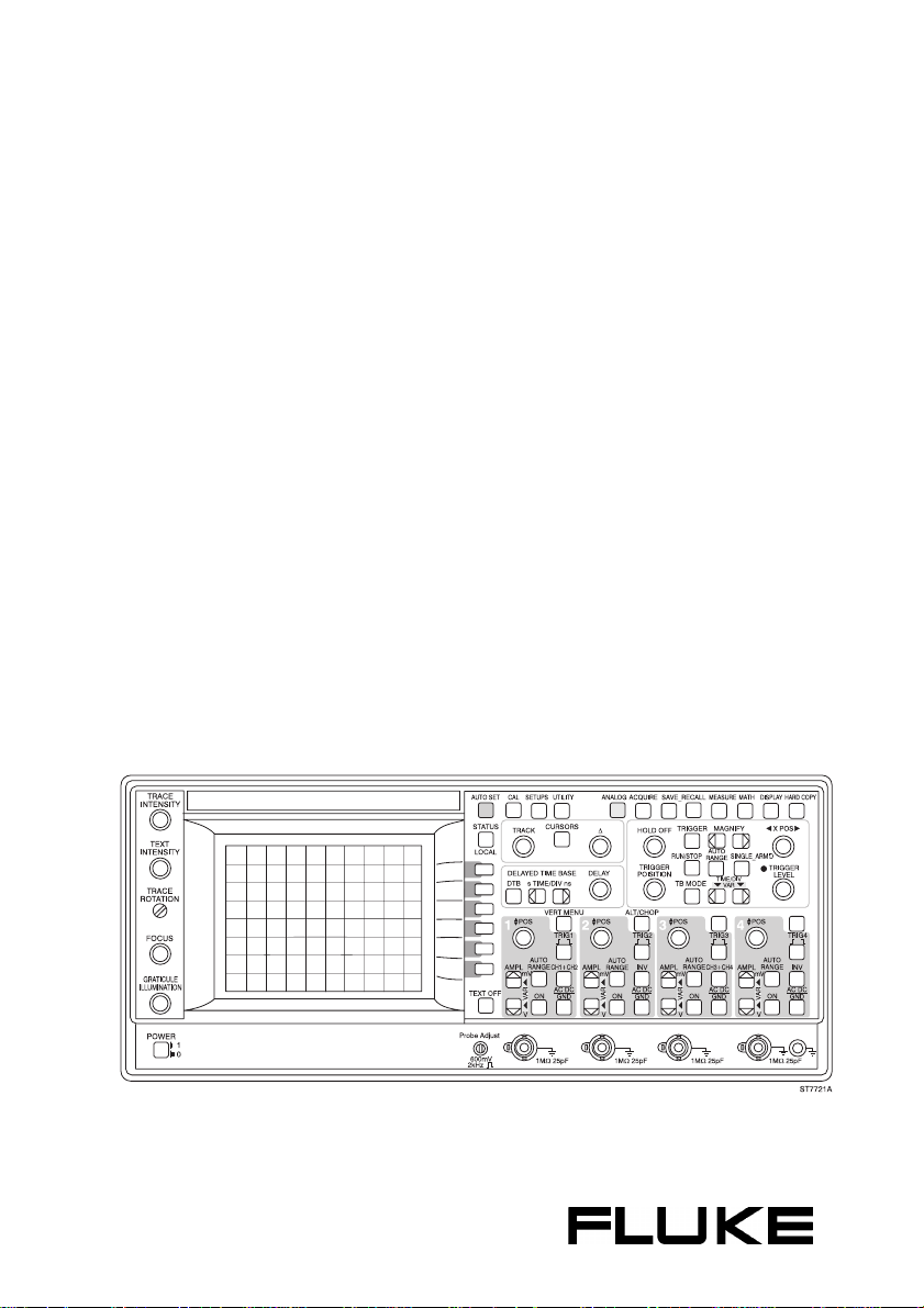
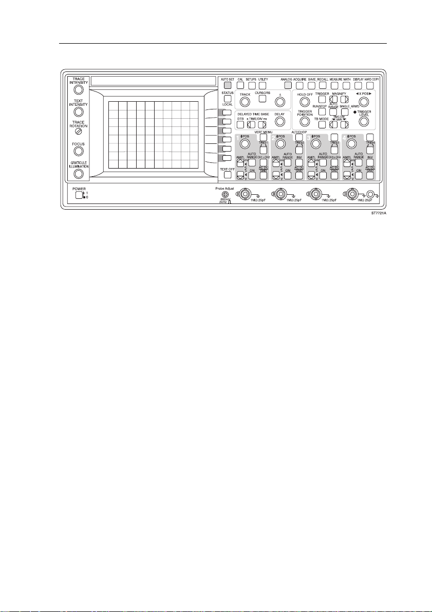
FRONT VIEW

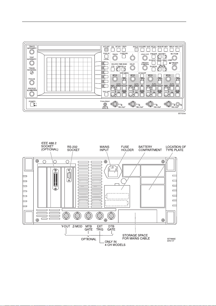
REAR VIEW

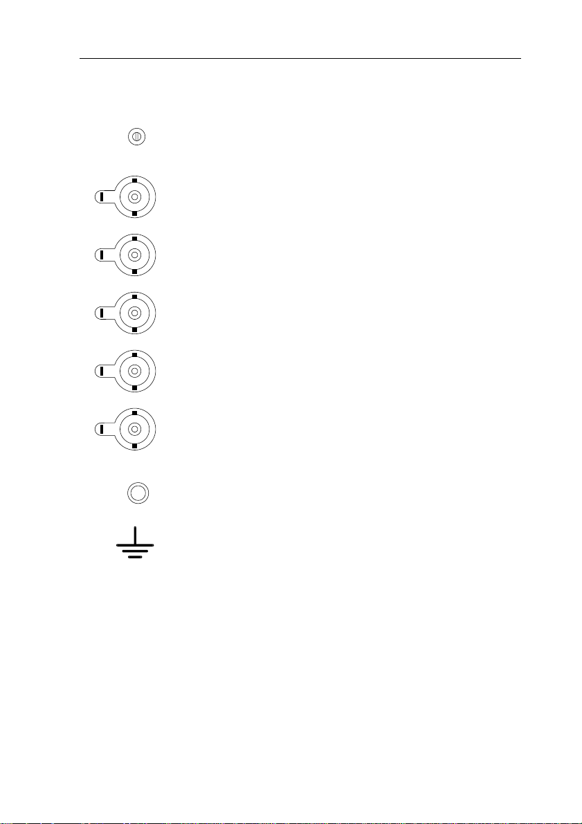
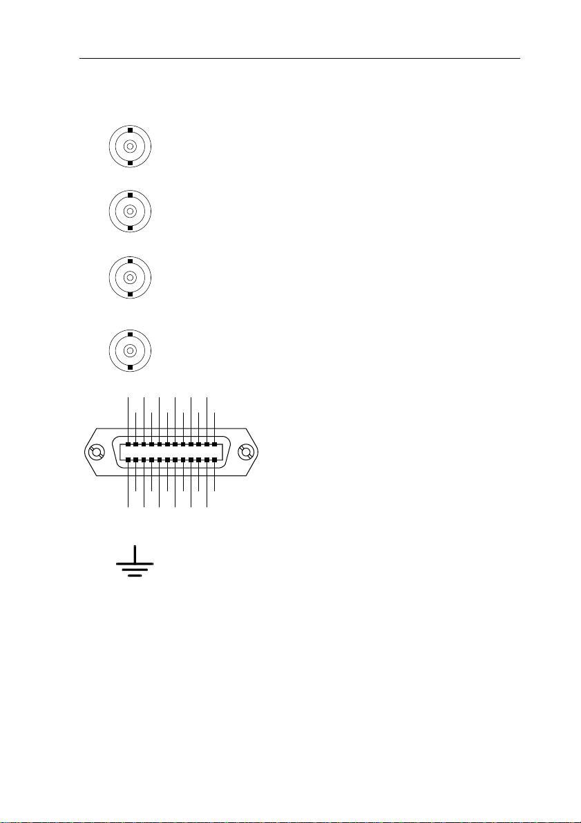
FRONT PANEL CONNECTIONS

Probe Adjust Squarewave output signal for e.g. probe calibration. Amplitude is calibrated.

CH1 BNC input socket for vertical channel 1 with probe indication contact.

CH2 BNC input socket for vertical channel 2 with probe indication contact.

CH3 BNC input socket for vertical channel 1 with probe indication contact. (only in 4 channel models)

CH4 BNC input socket for vertical channel 1 with probe indication contact. (only in 4 channel models)

EXT TRIG BNC input socket used as an extra external trigger input with probe indication contact (only in 2 channel models)

XIII

Ground socket (banana): same potential as safety ground.

The measuring ground socket and the external conductor of the BNC sockets are internally connected to the protective earth conductor of the three-core mains cable. The measuring ground socket or the external conductor of the BNC-sockets must not be used as a protective conductor terminal.

XIV

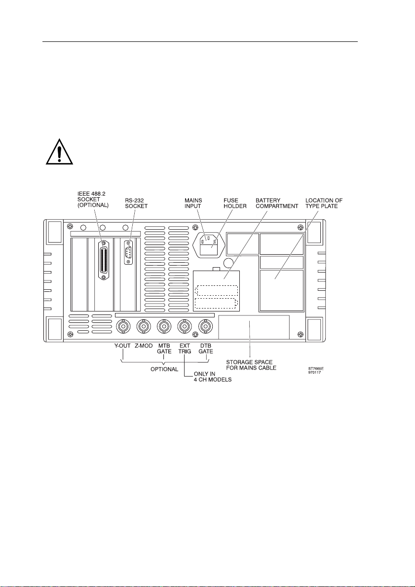
REAR PANEL CONNECTIONS

Z-MOD BNC input socket for external intensity-modulation of the CRT trace.

TXD

RXD

DTR

RS-232 BUS (EIA-232-D) Input/output socket to connect the oscilloscope to an RS-232 Interface.

LINE IN Line input socket. Fuse holder is built in.

RTS

CTS

ST6065

DSR

NC=NOT CONNECTED

FUSE

OPTIONAL REAR PANEL CONN ECTIONS

CH1 Y-OUT BNC output socket with a signal derived from the Channel 1 input signal.

MAIN TB GATE BNC output socket with a signal that is "high" when the Main Timebase i s running and "low" for the other conditions.

DTB GATE BNC output socket with a signal that is "high" when the Delayed Timebase is running and "low" for the other conditions.

EXT TRIG (only in 4 channel models) BNC input socket used as an extra external trigger input for the Main Timebase

DIO4

SHIELD

LOGIC

GND

SRQ

IFC

ATN

GND11GND

GND

NDAC

GND

GND8GND

DIO2

DAV

EO1

DIO3

DIO1

IEEE 488.2 BUS OPTION If installed you will find here the input/output socket to connect the oscilloscope to an IEEE 488 interface.

DIO7

REN

DIO5

DIO6

DIO8

ST6064

The external conductor of the BNC sockets and the screening of the interface bus connectors are internally connected to the protective earth conductor of the three-core mains cable. The external conductor of the BNC sockets and the screening of the interface bus connectors must not be used as a protective conductor terminal.

OPERATORS SAFETY 1 - 1

1 OPERATORS SAFETY

ATTENTION: The instrument is designed for indoor use only.

Read this page carefully before installation and use of the instrument.

1.1 INTRODUCTION

The instrument described in this manual is designed to be used by proper-lytrained personnel only. Adjustment, maintenance and repair of the exposed equipment shall be carried out only by qualified personnel.

1.2 SAFETY PRECAUTIONS

For the correct and safe use of this instrument it is essential that both operating and service personnel follow generally-accepted safe ty procedures in addition to the safety precautions specified in this manual. Specific warning and caution statements, where they apply, will be found throughout the manual. Where necessary, the warning and caution statements and/or symbols are marked on the apparatus.

1.3 CAUTION AND WARNING STATEMENTS

CAUTION: Is used to indicate correct operating or maintenance

procedures in order to prevent damage to or destruction of the equipment or other property.

WARNING: Calls attention to a potential danger that requires correct

procedures or practices in order to prevent personal injury.

1 - 2 OPERATORS SAFETY

1.4 SYMBOLS

Read the safety information in the manual.

Earth.

Conformité Européenne.

Recycling information.

1.5 IMPAIRED SAFETY PROTECTION

The use of the instrument in a manner not specified may impair the protection provided by the equipment. Before use, inspect the instrument and accessories for mechanical damage! Whenever it is likely that safety-protection has been impaired, the instrument must be made inoperative and be secured against any unintended op eration. The matter should then be referred to qualified technicians. Safe ty prote ction i s likely to be impaired when, for example, the instrument fails to perform the intended measurements or shows visible damage.

1.6 MEASURING EARTH

The measuring earth socket and the external conductor of the BNC sockets are internally connected to the protective earth conductor of the three-core mains cable. The measuring earth socket or the external condu ctor of the BNC-sockets must not be used to connect a protective conductor.

INSTALLATION INSTRUCTIONS 2 - 1

2 INSTALLATION INSTRUCTIONS

Attention: You are strongly advised to read this chapter thoroughly before

installing your oscilloscope.

2.1 SAFETY INSTRUCTIONS

2.1.1 Protective earthing

Before any connection to the input connectors is made, the instrument shall be connected to a protective earth conductor via the three-core mains cable; the mains plug shall be inserted only into a socket outlet provided with a protective earth contact. The protective action shall not be negated by the use of an extension cord without protective conductor.

WARNING: Any interruption of the protective conductor inside or outside

the instrument is likely to make the instrument dangerous. Intentional interruption is prohibited.

WARNING: When an instrument is brought from a cold into a warm

environment, condensation may cause a hazardous condition. Therefore, make sure that the grounding requirements are strictly adhered to.

2.1.2 Mains voltage cord, mains voltage range and fuses

Before inserting the mains plug into the mains socket, make sure that the instrument is suitable for the local mains voltage.

NOTE: When the mains plug has to be adapted to the local situat io n , such

adaption should be done by a qualified technician only.

WARNING: The instrument shall be disconnected from all voltage

sources when a fuse is to be renewed.

The oscilloscope has a tapless switched-mode power supply that covers most nominal voltage ranges in use: ac voltages from 100 ... 240 V (r.m.s.). This obviates the need to adapt to the local mains (line) voltage. The nominal mains (line) frequency range is 50 Hz ... 400 Hz.

Line fuse rating: 3.15 A T dela yed action, 250 V ( for ordering code see "INITIAL INSPECTION").

2 - 2 INSTALLATION INSTRUCTIONS

The mains (line) fuseholder is located on the rear panel in the mains (line) input socket. When the mains (line) fuse needs replacing, proceed as follows:

- disconnect the oscilloscope from the mains (line).

- remove the cover of the fuseholder by means of a small screwdriver.

- fit a new fuse of the correct rating and refit the cover of the fuseholder.

WARNING: Make sure that only fuses with the required rated current and

of the specified type are used for replacement. The use of makeshift fuses and the short-circuiting of fuse holders are prohibited.

REAR VIEW

Figure 2.1 Rear view of the instrument showing the mains input/fuse-holder

and back-up battery compartment.

When the apparatus is connected to its supply, terminals may be live, and the opening of covers or removal of parts (except those to which access can be gained by hand) is likely to expose live parts.

The apparatus shall be disconnected from all voltage so urces before it is opened for any replacement, maintenance or repair.

Capacitors inside the apparatus may still be charged even when the apparatus has been disconnected from all voltage sources.

Any maintenance and repair of the opened apparatus under voltage shall be avoided as far as possible and, when inevitable, shall be carried out only by a skilled person who is aware of the hazard involved.

INSTALLATION INSTRUCTIONS 2 - 3

2.2 MEMORY BACK-UP BATTERIES

2.2.1 General information

Memory backup is provided to store the oscilloscope’ s settings when switched off so that the instrument returns to the same settings when turned on. T wo AA (LR6) Alkaline batteries are used.

Note: The batteries are not factory installed and must be installed at the

customer’s site.

Note: This instrument contains batteries. Do not dispose of these batteries with

other solid waste. Used batteries should be disposed of by a qualified recycler or hazardous materials handler. Contact your authorized Fluke Service Center for recycling information.

2.2.2 Installation of batteries

Proceed as follows:

- Remove all input signals and disconnect the instrument line power.

- Remove the plastic cover of the battery compartment so that the battery holder becomes accessible.

- Install two penlight batteries (AA) in the battery holder as indicated on the battery holder.

- Reinstall the cover of the battery compartment.

Note: Frontsettings and autocalibration data disappear after exchange of the

batteries with the instrument disconnected from the line power. After battery exchange, it is necessery to press the CAL key after the recommended warming up time.

CAUTION: Never leave the batteries in the oscilloscope at ambient temper-

atures outside the rated range of the battery specifications because of possible damage that may be caused to the instrument. T o avoid batt ery damage, do not leave the bat teries in the oscilloscope when it is stored longer than 30 days.

2.3 THE FRONT COVER

For ease of removal and reinstallation, the front cover has been designed to snap on to the front of the instrument.

The front can be removed as follows:

- Fold the carrying handle down so that the oscilloscope occupies a sloping position (refer to Chapter 2.4 for how to proceed).

- Pull the clamping lip at the top side of the cover slightly outwards.

- Lift the cover off the instrument.

2 - 4 INSTALLATION INSTRUCTIONS

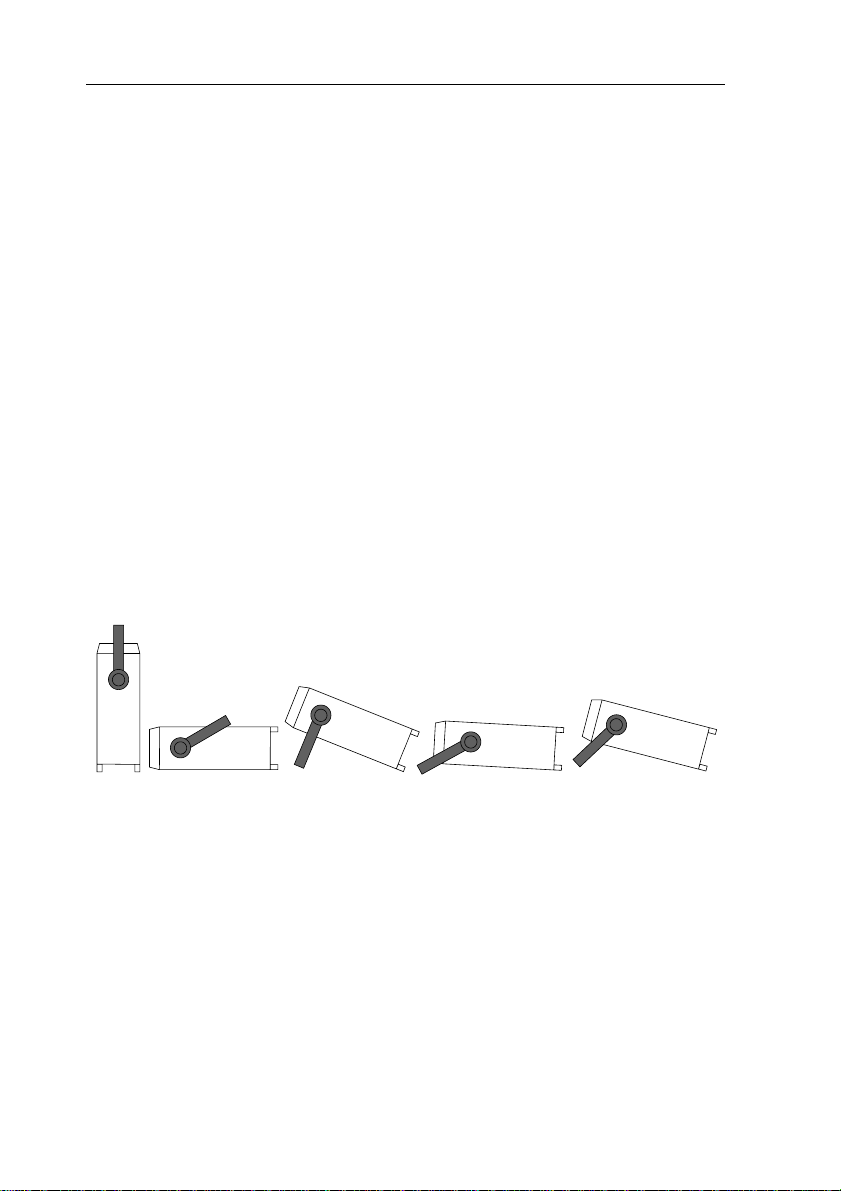
2.4 HANDLE ADJUSTMENT AND OPERATING POSITIONS OF THE INSTRUMENT

By pulling both handle ends outwards away from the instrument, the handle can be rotated to allow the following instrument positions:

- vertical position on its rear feet;

- horizontal position on its bottom feet;

- in three sloping positions on its handle.

The characteristics mentioned in the REFERENCE MANUAL are guaran teed for the specified positions or when the handle is folded down.

CAUTION: To avoid overheating, ensure that the ventilation holes in the

covers are free of obstruction. Do not position the instrument in direct sunlight or on any surface that produces or radiates heat.

In the rear panel of the instrument there is storage space for the mains cable. There is also a clamping device to fix the end of the mains cable to the re ar panel. The mains plug then fits in the area where the RS232 co nnector is present. In this way the instrument can also stand on its rear feet.

MAT4221

Figure 2.2 Instrument positions

2.5 IEEE 488.2/IEC 625 BUS INTERFACE OPTION

If your oscilloscope is equipped with the IEEE 488.2 interface, it can be used in a bus system configuration. The protocol used is SCPI (Standard Commands for Programmable Instruments). For setup information, refer to the function REMOTE CONTROL IEEE 488.2 in Chapter 5.

The IEEE 488.2 interface is a factory-installed op tio n.

INSTALLATION INSTRUCTIONS 2 - 5

2.6 RS-232-C SERIAL INTERFACE

Your oscilloscope is equipped with an RS-232-C interface as standard. The interface can be used in a system for serial communication. The protocol used is CPL (Compact Programming Language). CPL is a small set of very powerful commands that can be used for full remote control. Detailed information about this interface and the CPL protocol is given in Chapter 6 in this manual. For setup information, refer to the REMOTE CONTROL RS-232 function in Chapter 5 ’Function Reference’.

2.7 RACK MOUNTING

The rackmount kit (PM 8960/04) allows you to install the oscilloscope in a standard 19 inch rack.

It is not necessary to open the oscilloscope itself to mount the rackmount kit. Installation can be done easily by the user.

2.8 VERSIONS

The model number of your oscilloscope (e.g. PM33...) is indicated on the text strip above the CRT. This model number is also represented by the digits 6, 7, 8 and 9 of the 12- digit code on the type plate on the rear panel. The ’A’ or ’B’ series is indicated by a 1 or 2 on the 5th digit.

The instrument’s serial number is also given on the type plate. This numbe r consists of a six digit code preceeded by the characters ’DM’.

The instrument version can also be displayed on the CRT after having pressed menu key UTILITY and then softkey MAINTENANCE.

GETTING STARTED 3 - 1

3 GETTING STARTED

This chapter provides a 10-minute tutorial intended for those who are not familiar with Fluke oscilloscopes. Those who are already fami liar can skip this chapter and continue to Chapter 4.

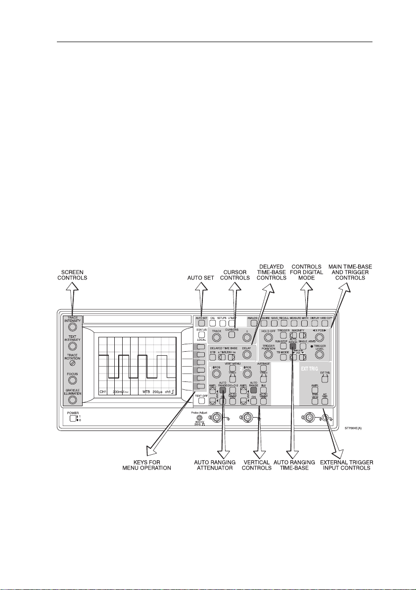
3.1 FRONT-PANEL LAYOUT

This oscilloscope is a combination of an analog oscilloscope and a digital storage oscilloscope in the same instrument. The basic signal acquisition and display functions are identical in both operating modes. Differences will be explained in the text. Switching between the two operating modes is done with the yellow ANALOG key.

The front panel of the oscilloscope is organized into functional areas. The areas are discussed in order of typical operation.

Figure 3.1 Front panel layout

Note that the front panel shown is that with the most functions. Differences are explained in Section 4.1. For this getting started procedure, only CH1 and CH2 are used. These are identical for all models.

3 - 2 GETTING STARTED

Typical operation of your instrument will be:

- Switching on the instrument (see Section 3.2)

- Initial standard setup (see Section 3.2)

- Screen controls (see Section 3.3)

- Auto setup (see Section 3.4)

- Analog-Digital mode switching (see Section 3.5)

- Vertical setup (see Section 3.6)

- Timebase setup (see Section 3.7)

- Magnify (Expand) (see Section 3.8)

- Direct trigger setup (see Section 3.9)

- Pretrigger view (see Section 3.10)

- More advanced features (see Section 3.11)

- Cursor operation (see Section 3.12)

- More advanced trigger functions (see Section 3.13)

- More signal detail with the DTB (see Section 3.14)

- Trace storage (see Section 3.15)

3.2 SWITCHING ON THE INSTRUMENT

Connect the power cord and set the front panel power switch to ON. For any line source between 100V to 240V nominal, 50/400 Hz, the instrument auto matically turns on. After performing the built-in power-up routine, the instrument is immediately ready for use. The instrument’s settings will be identical to those when the oscilloscope was switched off (with the batteries installed). To ensure that you will get the same setup in all cases, press the and

TEXT OFF

default condition (STANDARD SETUP) and a trace will appear on the screen. Text is also displayed at the bottom of the screen.

key simultaneously. This will set the instrument in a predefined

STATUS

key

GETTING STARTED 3 - 3

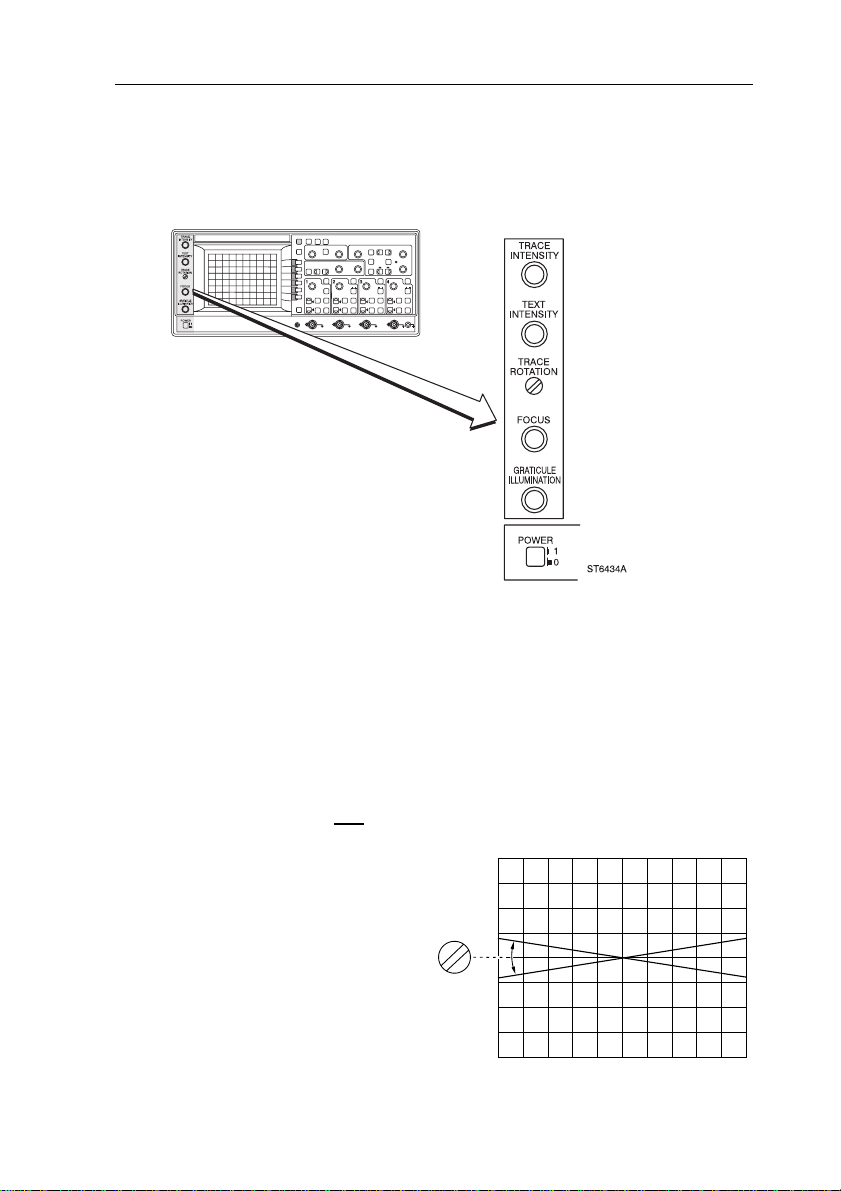
3.3 SCREEN CONTROLS

The screen controls can be adjusted for optimum trace, text and spot quality by the controls to the left of the screen.

Figure 3.2 Screen control area

The brightness on the screen is adjusted by two controls, one for the trace and one for the text.

• Turn the

TRACE INTENSITY

control clockwise and verify that only the

brightness of the trace increases.

• Turn the

TEXT INTENSITY

control clockwise and verify that only the

brightness of the text increases.

The sharpness of the trace and

text is optimized by the

When you are making photographs or are in a dark environment, you can use the

ILLUMINATION

control to illuminate the graticule of the screen.

The trace is adjusted in parallel with the horizontal graticule lines by the screwdriver-controlled

ROTATION

control.

TRACE

ROTATION

FOCUS

control.

ST5975

9303

3 - 4 GETTING STARTED

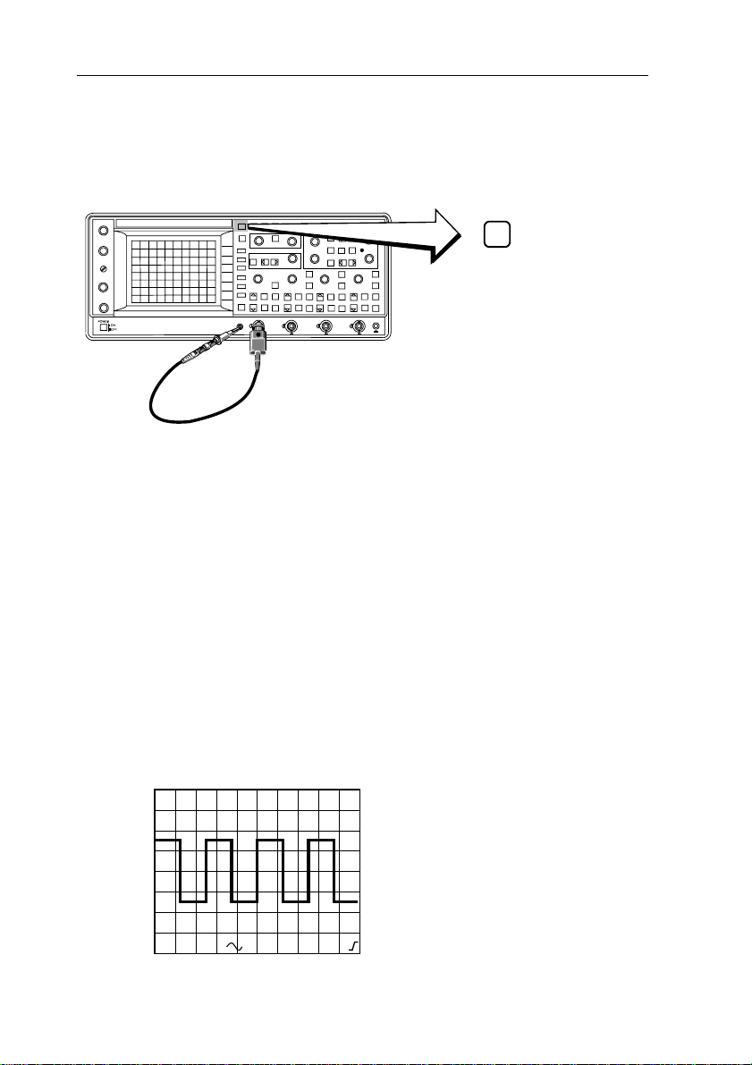
3.4 AUTO SETUP

The best way to start each measurement is by using the AUTOSET key. This

automatically

finds and scales all relevant parameters on all channels.

AUTO SET

ST6659

9303

Figure 3.3 Measuring setup

Step 1 Connect the probe as shown in figure 3.3.

NOTE: AUTOSET is programmable. Because you have set the instrument in the

"standard setup" before (see Section 3.2), all programmable features are set to a predefined condition an d the instrument is set in the analog mode . Programming of AUTOSET is explained in Chapte rs 4 and 5.

Step 2 Press the

AUTOSET

key.

The scope flashes the message ’AUTO SETTING...’ on the screen. In a few seconds the front-panel settings are adjusted for an optimized display of the applied signal in the analog mode.

Step 3 The calibration signal is clearly displayed.

The parameters of the channel and the timebase settings are displayed at the bottom of the screen.

CH1

200mV

MTB 200µs

CH1

ST6704

GETTING STARTED 3 - 5

Step 4 To prevent measurement errors, check the pulse response before any

measurement. If the pulse shows overshoot or undershoot, you can correct this by using the trimmer in the probe’s body. Chapter 4 describes how to adjust the pulse response.

ST5952

In most cases, using AUTO SETUP is sufficient for a good initial display of the signal(s). After the initial AUTOSET, and to optimize the signal for a more detailed view, continue with the paragraphs below.

NOTE: If you get lost when adjusting your instrument, just press AUTOSET.

3 - 6 GETTING STARTED

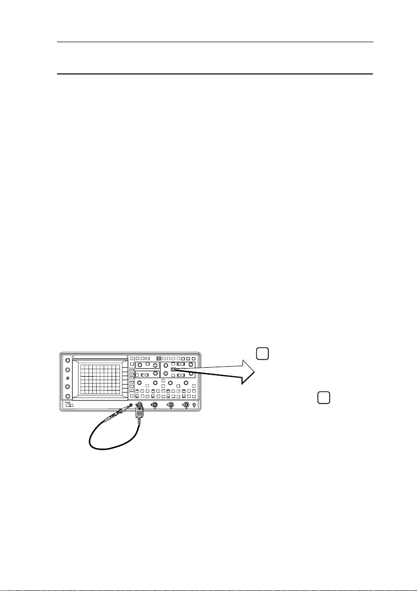
3.5 MODE SWITCHING BETWEEN ANALOG AND DIGITAL OPERATING MODES

Y ou can use the yellow ANALOG key to switch from the analog mode to the digital mode and back at any time. The signal acquisition and display functions of both operating modes are very similar. However, the nature of the signals you are using may determine which operating mode you prefer to use. For more information, refer to the following table:

SIGNAL CRITERIA ANALOG MODE DIGITAL MODE Repetitive signals of Usable Usable

30 Hz and higher Repetitive signals Causes display Preferred

below 30 Hz flickering Single events Displayed for the Can capture and

duration of display for long the event term display

Repetitive signals that are Preferred May cause alaising amplitude modulated Use Peak detect or

Envelope mode

Repetitive signals that Preferred May cause aliasing. are modulated in frequency Use Envelope mode.

Long serial data streams Preferred when When using delayed

Delayed sweep sweep to observe is not used. details, Digital mode

provides better light output.

Video signals Preferred when When using delayed

Delayed sweep sweep to observe is not used. details, Digital mode

provides better

light output. OTHER CRITERIA Need to see pretrigger Not possible Up to full acq uisition

information length

GETTING STARTED 3 - 7

SIGNAL CRITERIA ANALOG MODE DIGITAL MODE You need to make adjustments Fastest Slower

to the circuitry and watch display display the signal change update update

Automatic measurements Can’t use Fully implemented Signal Math Add, Subtract All functions

Add, Subtract, Multiply

Signal Analysis Not available Full analysis

Integration, (optional) Differentiation, FFT

Automatic Pass/Fail test Not available Fully implemented

(optional)

Autorange attenuator Not available Results in a displayed

signal with an amplitude of 2 to 6.4 divisions

Autorange timebase Not available Results in a signal

display of 2 to 6 waveform periods

ANALOG

RUN/STOP

ST6680

9312

Figure 3.4 Analog-Digital switching setup

Step 1 Press AUTOSET. The scope performs an AUTOSET in analog mode. Step 2 Press the ANALOG key to change over to the digital mode. Check that

the picture is identical to the one in the analog mode. The text ’DIGIT AL MODE’ is displayed briefly at the bottom of the screen.

3 - 8 GETTING STARTED

Step 3 Press AUTOSET again. This time the scope performs the autoset in

digital mode.

Step 4 Press the RUN/STOP key and observe that the trace is frozen and

stays on screen even after removing the probe.

Step 5 Press the RUN/STOP key to display the actual input signal again.

Reconnect the probe to display the Probe Adjust signal again.

Step 6 Press the ANALOG button once again to return to the analog mode. In

the bottom of the screen, the text ’ANALOG MODE‘ is briefly displa yed.

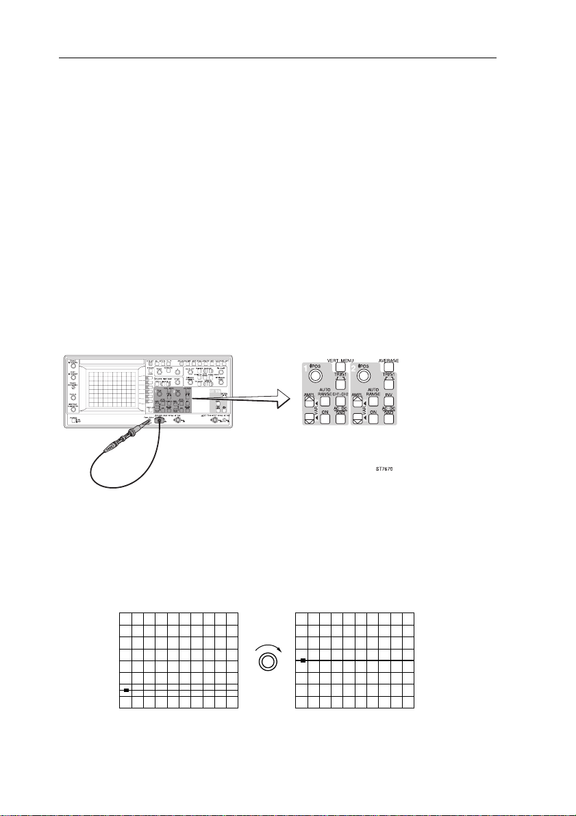
3.6 VERTICAL SETUP

This section deals with setting of the input circui ts of the four channels. The ma in adjustments are AMPLitude, POSition, and the channel input coupling selection for GND, DC, and AC.

Figure 3.5 Vertical setup

Step 1 Adjust the absolute ground level by disconnecting the signal and using

the POS control to position the trace in the middle of the screen. A marker with the channel number (’1-’) at the left of the screen indicates the ground reference.

POS

MAT4191

Step 2 Reconnect the probe to the Probe Adjust signal for display.

GETTING STARTED 3 - 9

CH1

100mV

CH1

500mV

ST6681

Step 3 You can change the amplitude of the signal in a 1, 2, 5 sequence by

pressing one of the AMPL keys. Note that the bottom of the screen shows the AMPL/DIV setting of CH1.

Step 4 Press the ON button of CH2 and observe that a second trace is now

visible. The position and amplitude of this channel can be adjusted similar to the adjustment of CH1. The channel settings are also displayed in the bottom of the screen.

Press the ON key of CH2 once again to turn this channel off.

Step 5 Press the AC DC/GND key of CH1 so that a ’⊥’ sign is displayed in the

bottom text line. This interrupts the input sig nal and connects the inpu t to the ground. In this case, only the ’base’ line is visible.

Press the AC DC/GND key once again for ac input coupling; the bottom text line now displays ’~’.

In most cases, dc input coupling is used to show ac as well as dc components of the signal. However, in some case s where a small ac sign al is superimp osed on a large dc voltage, ac input coupling must be used. Then only the ac component is visible on the screen. The text line shows a ’=’ or ’~’ sign to indicate dc or ac coupling. Because the calibration signal is a square wave with a low level of 0V and a high level of +600 mV , the screen sh ows either of the following two displays:

AC INPUT COUPLING

ZERO

LEVEL

CH1

200mV

MTB 200µs

CH1

DC INPUT COUPLING

ZERO

LEVEL

CH1

200mV

MTB 200µs

CH1

ST6682

3 - 10 GETTING STARTED

Step 6 Press the ANALOG key to enter the digital mode Step 7 Press the top one (mV) of the AMPL keys, so that the signal has

maximum amplitude. Press AUTO RANGE and see the signal change to a suitable

attenuator value. When AUTO RANGE is active, the attenuators automatically adjust when the signal amplitude changes, to keep the trace on screen.

Step 8 Press the key labeled AVERAGE. Noise in the input signal can be

reduced by using the average function. The random noise is reduced by calculating the average over the last n scans (average factor ca n be set between 2 and 4096)

NOTE: Refer to Chapter 4 for an explanation of the CH1+CH2, TRIG1, and

INV keys.

GETTING STARTED 3 - 11

ST6683

MTB 100µsMTB 500µs

TIME/DIV

3.7 TIMEBASE SETUP

The next step is the adjustment of the main timebase controls (

POS

ition, and

MAGNIFY

keys).

MAGNIFY

AUTO

RANGE

TIME/DIV

sns

Figure 3.6 Timebase setup

Step 1 Press the Step 2 Use the

AUTOSET

TIME/DIV

key.

keys on the right hand side of the instrument to decrease or increase the number of periods of the signal on the screen.

TIME/DIV, X

VAR

XPOS

ST6435

9312

Step 3 Select a timebase of 1 ms/div. Step 4 Press

AUTO RANGE

and see the signal display change to a more suitable timebase. The AUTO RANGE function au tomatically selects a timebase that displays 2 to 6 signal periods.

Step 5 Press the Step 6 Turn the

ANALOG

X POS

key to switch the scope to the analog mode.

control to shift the signal horizontally (left or right)

across the screen.

3 - 12 GETTING STARTED

3.8 MAGNIFY (EXPAND)

Step 1 You can use the

MAGNIFY

keys to expand the signal on the screen. The ’MGN’ indication and the corrected timebase settin g are displayed in the text line. In the analog mode, magnification is limited to activate the magnification. The left key will turn off the MAGNIFY

10. The right key will

function. On or off is indicated by ’MGN’ in the bottom of the screen.

Step 2 Press the

ANALOG

Step 3 In the digital mode, pressing the right

signal in left operate the

1, *2, *4 ...steps to a maximum of *32 times. Pressing the

MAGNIFY

key to switch the scope to the digital mode.

MAGNIFY

key compresses the signal to

buttons, or when you turn the X

key expands the

1 again. When you

POS

ition control, a bargraph is displayed showing whic h part of the digital trace is expanded.

NOTE: The MAGNIFY key and X POS control can also be used after the

oscilloscope is STOPped.

5.00µs

10 DIV

1.25µs

10 DIV

START OF TIME WINDOW CAN BE VARIED WITH XPOSOVER THE WHOLE SWEEP RANGE.

1.00ms 40 DIV

ST6684

GETTING STARTED 3 - 13

3.9 DIRECT TRIGGER SETUP

Now you are ready to set your trigger conditions. Y ou will use one of the channel selection keys (

control.

LEVEL

TRIG1, TRIG2, TRIG3, TRIG4 or EXT TRIG

Figure 3.7 Direct trigger setup

) and the

TRIGGER

Step 1 Press the

output is now displayed on channel 1. Turn chann el 2 on to display a second horizontal trace (channel 2 has no input signal).

Step 2 Press the

source. The result is that the signal on channel 1 is no longer triggered (not stable). The not triggered. Check also that the right side of the bottom text line indicates the trigger source (’ch2’).

Step 3 Only in 2 channel models

Press source. Check that the rightside of the bottom textline indicates the trigger source ’EXT’.

Step 4 Press the

The ’ch1’ symbol is displayed in the bottom text line. Triggering resumes. Turn channel 2 off, by pressing ON again.

Step 5 Press the ns key of the MainTB

set to ’2 µs/div’.

AUTOSET

TRIG2

EXT TRIG

TRIG1

key. The square-wave signal of the Probe Adjust

key so that channel 2 is selected as the trigger

LED is on, to indicate that the oscilloscope is

ARM’D

key to select External Trigger input as the trigger

key. Channel 1 is now selected as the trigger source.

TIME/DIV

keys until the timebase is

3 - 14 GETTING STARTED

Step 6 The same TRIG1 key that was used to select the trigger source is also

used to select the trigger slope. Repeatedly pressing the TRIG1 button changes the triggering so that it occurs on the leadin g o r tr aili ng edge of the input signal. Note that the slope is also displayed in the bottom text line.

TRIG1

MTB 2µs

CH1

200mV

CH1

200mV

MTB 2µs

CH1

ST6685

Step 7 For repetitive signals, you obtain a stable display when each

successive timebase sweep is triggered at the same stable level of the input signal. You use the TRIGGER LEVEL control to adjust the level. Turn the control. The precise positio n in relation to the maximum signal amplitude (between +100 % and -100 %) is displayed on the screen.

SUMMARY The previous steps covered the basic adjustments. Now you are ready to look at the special features of the oscilloscope. This includes the use of the cursors, advanced trigger functions and using the second (delayed) timebase for signal details.

GETTING STARTED 3 - 15

3.10 PRE-TRIGGER VIEW

One of the powerful features in the digital mode is the ability to capture and view signal contents prior to the actual trigger. The amount of pretrigger information can be as long as one full acquisition/record. The trigger position is ad justed with the

TRIGGER POSITION

control.

Step 1 Turn the

triggering edge shifts to the center of the screen. A trigger point marker (s) indicates the trigger point. The part to the left o f the marker is called pretrigger view. The pretrigger view is indicated in the bottom of the screen (in divisions)

Step 2 The

TRIGGER POSITION

delay. Rotate the readout displays "0". When you continue to turn the TRIGGER POSITION control clockwise, a positive delay between trigger point and acquisition is set. The delay is no longer read out in divisions of pretrigger information, but in seconds, or fractions of seconds to indicate how much delay is used.

TRIGGER POSITION

control can also be used to adjust time

TRIGGER POSITION

control counter clockwise. Now the

DELAY=−5.00dV

PRE-TRIGGER VIEW

ST6686

control clockwise until the

3 - 16 GETTING STARTED

3.11 MORE ADVANCED FEATURES

All basic functions are accessed by dedicated keys for fast and easy operation. Some of the more advanced features are menu operated. Menu s are called up by pressing one of the keys identified with press one of these keys, a menu is displayed on the right side of th e screen. This menu gives you access to the more advanced functions of the oscilloscope. Use the blue softkeys to the right of the screen to select the desired functions; the selected function is indicated by the highlighted text.

SOFTKEYS

Figure 3.8 Menu keys and softkeys

text on the front panel. After you

blue

TRIGGER WITH MENUKEY

TRIGGER

ST6433

9303

Step 1 Press the key marked

TRIGGER

. Check that the ’TRIGGER MAINTB’ menu is displayed at the right side of the screen.

After changing the setting, you can deactivate the menu again to use the full screen for the signal. There are two ways to do this:

- Press the

TRIGGER TEXT OFF

key once again.

key. The TEXT OFF key operates in a 1-2-3 cycle, and allows you to blank the bottom text line as well.

TRIGGER MAIN TB

edge tv logic

ch1

line

TEXT OFF

CH1

MTB 200µs

200mV

CH1

200mV

MTB 200µs

TEXT OFF

CH1

Step 2 Use both methods to familiarize yourself with turning the menus and

the bottom text line on and off.

ST6679

GETTING STARTED 3 - 17

3.12 CURSOR OPERATION

Cursors are used for accurate amplitude or time measurements of the signal.

TRACK

CURSORS

∆

ST6431

9303

Figure 3.9 Cursor setup

Step 1 Before you continue, reset the instrument with the STANDARD

SETUP. To do this, press the

STATUS

key and

TEXT OFF

key simultaneously. Now the instrument is set in the default condition and operates in analog mode.

Step 2 Press the Step 3 Press the

AUTOSET

CURSORS

key.

key to enter the cursors menu.

CURSORS

The menu is now displayed on the screen and the cursors are turned on.

on off

Step 4 Use the second blue softkey from the top to select

one of the three cursor modes:

- Amplitude cursor measurements, indicated by ’=’.

- Time cursor measurements, indicated by ’||’ for

measuring time or frequency.

- Amplitude

’#’. The top text line displays the result of the

time measurements, indicated by

and

READ OUT

measurements (∆V or ∆T).

Step 5 Press the second bluesoft key until ’||’ is highlighted.

ST6430

Step 6 The

TRACK

control moves both cursors at the same time. For example, to measure the period time of the input signal, set the left (reference) cursor to a rising edge of the signal.

Step 7 The ∆ contro l moves the right cursor only . Set this cursor the next rising

edge of the signal.

3 - 18 GETTING STARTED

Step 8 The top text line now shows the pulse repetition time of the signal

(e.g., ch1: ∆T= 500 µs).

200µs

CURSORS

on off

READ OUT

CH1

ST6687

ch1:

∆T= 500µs

CH1 200mV

MTB

Step 9 Press the second blue softkey until ’=’ is highlighted. Now perform a

peak-to-peak measurement and check that th e amplitude of the signal (’∆V’) is 600 mV.

NOTE: When you select ’#’, the fifth blue softkey is automatically activated so

that you can choose between using the controls for positioning the vertical cursors (’||’) or the horizontal cursors (’=’).

The ’READOUT’ submenu is explained in Chapter 4. Step 10 Select the vertical cursors again. Step 1 1 Now switch to the digital mode. Notice the changing readout and the

’X’ indicating where the trace and the cursors intersec t. Since the trace is digitized, the cursors can be really smart. In the digital mode you can measure time differences (∆T) and amplitude differences (∆V) at the same time.

200µs

CURSORS

on off

ch1

READ OUT

CH1

ST6688

9303

ch1:

∆T= 500µs

CH1 200mV

∆V= 600mV

MTB

Step 12 Use the first blue softkey to turn the cursors off. The cursor menu

disappears.

GETTING STARTED 3 - 19

3.13 MORE ADVANCED TRIGGER FUNCTIONS

Most of the trigger functions (source, slope, and level) can be controlled with direct access to the functions (see Section 3.9). A CRT menu is used for more advanced trigger functions.

TRIGGER

TB MODE

ARM’D

TRIGGER

LEVEL

ST6432

9303

Figure 3.10 More advanced trigger setup

Press the menu key

TRIGGER

. This turns the menu on. An extensive set of functions is now displayed.

All functions are explained in Chapter 4. For most applications, this menu is not needed.

3 - 20 GETTING STARTED

3.14 MORE SIGNAL DETAIL WITH THE DELAYED TIMEBASE

When you need to study a part of a signal in more detail, a second (delayed) timebase is available. This timebase has its own timebase settings and trigger level adjustment. Additional selections are made in the DELAYED TIMEBASE menu.

DISPLAY

MAGNIFY

Figure 3.11 Delayed timebase setup

Step 1 Press the

STATUS

key and STANDARD SETUP. Then shift to trace to the upper half of the screen as indicated.

50mV

CH1

MTB 1.00ms

DELAYED TIMEBASE

DTB

sns

TIME/DIV

TEXT OFF

ch1

ST6690

TRIGGER

DELAY

POSITION

TB MODE

key at the same time for

ST6439

9303

GETTING STARTED 3 - 21

Step 2 Press the DTB key . The DELA YED TIME BASE menu is now displayed

on screen. Turn the delayed time base on with the first softkey.

DELAYED TIME BASE

DEL’D TB on off

MAIN TB

on off starts

trig’d

TRACE

SEP

CH1

50mV

MTB1.00ms

DTB 100µs4.882ms

ch1

ST6689

The upper trace is the main timebase trace. This first trace shows an intensified part. Adjust the TRACE INTENSITY with the control as necessary. The lower trace is the delayed timebase trace and is an expanded representation of the intensified part in the upper trace.

Step 3 Turn the DELAY knob to shift the intensified part and to select which

part of the main timebase you want to magnify.

Step 4 The delayed timebase TIME/DIV keys are used to select the

’magnification factor’. Notice the changing delayed timebase ’TIME/ DIV’ readout at the bottom of the screen.

Step 5 The ’T’ symbol at the fourth blue softkey indicates that the cursor

TRACK control can be used to make adjustments. In this menu the cursor TRACK control is used to change the TRACE SEParation, which is the distance between the main timebase and the delayed timebase.

The delayed timebase can be used in the triggered mode. The trigger ed mode is selected with the STARTS/TRIG’D softkey . The function of the triggered mode will be explained in Chapter 4. For this part of "Getting Started", remain in the STARTS mode.

Step 6 Switch the menu off with the TEXT OFF key. Notice that the delayed

timebase is still active and that the most important functions (DELAY control and TIME/DIV key pair) still allow you to operate the delayed timebase.

3 - 22 GETTING STARTED

3.15 TRACE STORAGE

In the digital mode you not only have the ability to store traces on the screen (using the

RUN/STOP

key), but also to store traces in memory for later use.

ANALOG

SAVE

RECALL

RUN/STOP

ST6691

9312

Figure 3.12 Digital memory setup

Store traces on screen: Step 1 Press

AUTOSET

Step 2 Make sure that the scope is in the digital mode. If not, press the

ANALOG

Step 3 With the

key to enter the digital mode.

RUN/STOP

key , new acquisitions are stopped and the display is frozen. Removing the input signal or pressing a key has no ef fect on the display . Stopping the acquisition is very useful to do me asurements on the signal or to make a hard copy.

Step 4 Press the

RUN/STOP

key to reactivate the acquisition.

Store traces in memory: Step 5 For this step-by-step introduction you will first clear all memory

locations so that all unnecessary traces are removed.

- press the

- select

CLEAR & PROTECT CLEAR ALL

- in the confirm menu, select Sometimes there will be a second confirm menu. Select

SAVE

menu key.

YES

again to

YES

clear protected traces as well. Press the

TEXT OFF

key to turn the menu off.

GETTING STARTED 3 - 23

Here is how traces are stored in memory: Step 6 Use the TRACK control to select an empty memo ry

location such as m1, m2, or m3. Empty locations are marked with a circle in front of the memory location number (e.g., m3).

Step 7 Press the second blue softkey (’save’). You have

now saved the acquisition signal into memory ’register’ m3. A single register can contain a set of up to three traces (e.g., CH1, CH2, and EXT (trigger view)). In this case only one input channel was

SAVE ACQ TO MEMORY

m2 m3 m4

save

clear

copy

turned on, so that only one was stored.

Step 8 Remove the probe from CH1. Now recall the stored

trace.

Step 9 Press the RECALL key.

CLEAR & PROTECT

ST6705

Step 10 Select the previously filled memory register m3 with the TRACK

control. A memory register with trace information is indicated with

Step 11 Press the second blue softkey to turn on the display of this register.

Indicated by

Step 12 Turn the ∆ control to separate the acquisition (live signal) and the trace

recalled from memory.

NOTE: You are now able to operate nearly all the oscilloscope’s functions in

most routine applications. Please continue with Chapter 4 for a more detailed description of the oscilloscope’s many advanced features.

Memory indications:

Empty register Filled register Displayed register

HOW TO USE THE INSTRUMENT 4 - 1

4 HOW TO USE MORE ADVANCED

FUNCTIONS OF THE INSTRUMENT

This chapter allows more experienced oscilloscope users to learn more about the advanced features of this instrument and how to use them. For a complete description of each function, refer to the next chapter in this manual: "Function Reference". This chapter explains the basics of each function and gives examples are given in a step by step sequence. Less experienced oscilloscope users should read Chapter 3 before beginning this chapter.

4.1 INTRODUCTION

All of the oscilloscope models in the PM337xB, PM338xB and PM339xB family combine the features and operation of an analog oscilloscope with that of a fullfeatured Digital Storage Oscilloscope (DSO). Switching between one mode of operation to the other is done by pressing one (yellow) push button. Most signal acquisition functions are identical for both modes of operation, even though the digital mode allows for pretrigger acquisition and display, plus more powerful logic triggering. Delayed sweep operation is available in both operating modes. Cursors operate in both modes. The digital mode provides access to many powerful calcul ated measurement and signal analysis functions. It also has a completely new feature called AUTO RANGE. AUTO RANGE automatically adjusts the attenuator or the timebase setting when the amplitude or the frequency of the signal has changed.

This family of oscilloscopes is available with a 60 MHz, 100 MHz or 200 MHz bandwidth. There are full four-channel instruments as well as 2+2 channel models. The economy version have 2 full channels and an external trigger channel.

PM3394B 200 MHz Full Four Channel Oscilloscope.

The PM3394B offers a 200 MHz bandwidth. Four channels provide equal bandwidth, and sensitivity ranges. Each channel has full AC/DC/GND coupling capabilities. In VERTMENU each channel is set to 50Ω or 1 MΩ input impedance.

4 - 2 HOW TO USE THE INSTRUMENT

PM3390B 200 MHz 2 Channel Oscilloscope

The PM3390B has the same capabilities as the PM3394B on the channels 1 and

2. The channels 3 and 4 are replaced by an externa l trigger channel. This channel can only be used as an additional trigger input channel. Signal manipulation as in the full channels 1 and 2 is not possible. The external trigger signal can be displayed by using the function TRIG VIEW.

PM3384B 100 MHz Full Four-Channel Oscilloscope

Bandwidth is 100 MHz. The PM3384B has the same capabilities as the PM3394B. VERT MENU only offers BW LIMIT selection.

PM3380B 100 MHz 2 Channel Oscilloscope

The PM3380B has the same capabilities as the PM3384B on the channels 1 and

2. The channels 3 and 4 are replaced by an external trigger channel as in the PM3390B. VERT Menu offers only BWLIMIT selection.

PM3370B 60 MHz 2 Channel Oscilloscope

The PM3370B has a bandwidth of 60 MHz. All other features are equal to those of the PM3380B.

HOW TO USE THE INSTRUMENT 4 - 3

FRONT PANEL LAYOUT

The controls on the front panel are grouped by function. In this chapter, a description for each group of controls is given in the following sequence:

- Display and probe adjustment (see section 4.2)

- Analog and digital modes (see section 4.3)

- Vertical deflection ( see section 4. 4)

- Horizontal deflection and triggering (see section 4.5)

- Digital acquisition and storage (see section 4.6)

- Advanced vertical functions (see section 4.7)

- Advanced horizontal and trigger functions (see section 4.8)

- Memory functions (see section 4.9)

- Cursor functions (see section 4.10)

- Measurement functions (see section 4.11)

- Processing functions (see section 4.12)

- Display functions (see section 4.13)

- Delayed timebase (see section 4.14)

- Hard copy facilities (see section 4.15)

- AUTOSET and other utilities (see section 4.16)

4 - 4 HOW TO USE THE INSTRUMENT

Study the front panel of your oscilloscope and observe what functions the different controls and push buttons (keys) perform. There are three differ ent styles of push buttons, plus the blue softkeys adjacent to the screen. The push button functions are as follows:

Direct function key. These keys provide direct access to specific functions as labeled on the front panel. Examples include AUTOSET for automatic setup of the oscilloscope and AC DC (GND) for selection of the instrument’s input coupling.

Menu initialization key, with blue text. Press to produce a menu on the screen from which you can select functions that are related to the function name of this key.

Key pair. These pair s serve as up/down controls. They a re used to select a value from a range.

Softkey. Press to select a function from the menu that has been initialized by pressing one of the menu initialization keys.

Rotary control. Used for continuously variable contr ol of a function.

HOW TO USE THE INSTRUMENT 4 - 5

4.2 DISPLAY AND PROBE ADJUSTMENTS

T o help you follow the step-by-step descriptions, each section begi ns by recalling the standard setting as outlined below. If you get "lost", you can return to the beginning of each section, because all functions are set to a predefined state to create a correct start situation.

RECALL STANDARD SETTING

- Simultaneously press the STA TUS and TEXT OFF keys.

Recalling the standard setting always results in a trace on the display, even with no signal applied to the oscilloscope inputs. Refer for a list of the standard setting to the section "STA NDARD SETUP/FRONT PANEL RESET" of Chapter 5.

DISPLAY ADJUSTMENT

Before going through the examples that introduce you to features of this oscilloscope, adjust the display as follows:

- Turn the TRACE INTENSITY control for optimum trace brightness.

- Turn the TEXT INTENSITY control for optimum display brightness of the text.

- Adjust trace alignment with the graticule by using the screwdriver control TRACE ROTATION.

- Turn the FOCUS control until a sharp trace is obtained.

- You can turn the GRATICULE ILLUMINATION control to illuminate the graticule lines as desired.

4 - 6 HOW TO USE THE INSTRUMENT

DISPLAY LAYOUT

The following illustration shows the layout of th e display with a maximum amou nt of text. Most text is active only when specific functions are activated.

HOW TO USE THE INSTRUMENT 4 - 7

MENUS TEXT OFF

A menu appears when a key with blue text is pressed. The menu functions can be selected by pressing the blue softkeys to the right side of the screen.

- Press the ANALOG key to select the digital mode.

- Press the DISPLAY key to activate the menu.

DISPLAY

Each menu starts with a menu name, which corresponds with the key that was used to select the menu. This is sometimes followed by a second name of the softkey that initialized a submenu.

WINDOWS

on off VERT MAGNIFY

off

XvsY

The windows function can be switched on and off by pressing the corresponding blue softkey.

indicates that a selection must be made with the

TRACK control. The arrow ( ) behind TEXT indicates that there is a

TEXT

submenu.

dots

linear

sine

ST7415

9312

The bottom softkey switches (toggles) between the three functions.

Y ou can turn of f the text by pressing the TEXT OFF key. This can be done to free up the display area.

- Press the TEXT OFF key three times.

Observe that the text mode follows the following sequence: menu off, settings of f, both on.

4 - 8 HOW TO USE THE INSTRUMENT

CAL SIGNAL AND PROBE ADJUSTMENT

Each measuring probe has been checked and adjusted before delivery. However, to match the probe to your oscilloscope, you must perform the following procedure to optimize the pulse response of the combination of oscilloscope input and probes.

- Connect the probe body to channel 1.

- Connect the probe tip to the Probe Adjust output of the oscilloscope.

- Press the AUTOSET key.

If the display looks like one of the two displays shown on the left, you must adjust your probe to get the display shown on the right. The probe output impedance can be adjusted through a hole in the compensation box of the probe to obtain optimum pulse response. Refer to the following figure.

ST6024

9303

- Adjust the probe until the screen shows the correct compensation.

The probe is now adjusted for optimum pulse response with this oscilloscope. If you connect the probe to another channel or oscilloscope, it must be adjusted again to that oscilloscope input.

- Repeat this adjustment for the second probe.

HOW TO USE THE INSTRUMENT 4 - 9

4.3 ANALOG AND DIGITAL MODES

ANALOG

This instrument is a combination of an analog real-time oscilloscope and a digital storage oscilloscope, which offers a variety of additional features. The combination of analog and digital modes in one instrument gives you the advantages of both modes.

In the

ANALOG MODE

the signal is directly written on the screen. The result is the "traditional" real-time signal representation. Because of the high update rate and infinite resolution, this image gives signal details that are vi sible on ly on tr ue analog oscilloscopes.

In the

DIGITAL MODE

the input signal is sampled. These samples are stored in memory so that mathematics, calculated measurements, printing, and other memory functions can be performed on the trace.

You can use the yellow ANALOG push button to switch from the analog mode to the digital mode and back at any time. The signal acquisition and displa y functions of both operating modes are very similar. However, the nature of the signals you are using may determine which operating mode you prefer to use. For more information, refer to the following table:

SIGNAL CRITERIA ANALOG MODE DIGITAL MODE Repetitive signals of Usable Usable

30 Hz and higher Repetitive signals Causes display Preferred

below 30 Hz flickering Single events Display for Can capture and

duration of display for long the event term

Repetitive signals that Preferred May cause aliasing. are amplitude modulated Use Peak detect or

Envelope mode

Repetitive signals that Preferred May cause aliasing. are modulated in frequency Use Envelope mode.

Long serial data streams Preferred when When using delayed

Delayed sweep sweep to observe is not used. details, Digital mode

provides better light output.

4 - 10 HOW TO USE THE INSTRUMENT

SIGNAL CRITERIA ANALOG MODE DIGITAL MODE Video signals Preferred when When using delayed

Delayed sweep sweep to observe is not used. details, Digital mode

provides better light output.

OTHER CRITERIA Need to see pretrigger Not possible Up to one screen

information You need to make adjustments Fastest Slower display

to the circuitry and watch display update update the signal change

Automatic measurements Can’t use Fully implemented Signal Math Add, Subtract only All functions

Add, Subtract, Multiply

Signal Analysis Not available Full analysis, with

Integration, Math Plus option Differentiation, FFT installed

Automatic Pass/Fail test Not available Fully implemented,

with Math Plus option installed

Autorange attenuator Not available Results in a

displayed signal with an amplitude of 2 to

6.4 divisions

Autorange timebase Not Available Results in a signal

display of 2 to 6 waveform periods

HOW TO USE THE INSTRUMENT 4 - 11

STANDARD SETTING

- Simultaneously press the STA TUS and TEXT OFF keys.

- Connect the Probe Adjust signal to channel 1.

The Probe Adjust signal, now supplied to the input, is a square wave with a lower level of 0V and a top level of 600 mV . The osci lloscope always operates in analog mode after a recall of the standard setting.

- Press the AUTOSET key for optimum signal display.

ANALOG TO DIGITAL MODE SWITCHING

Switching from analog to digital mode and vice-versa can be done by pressing the yellow

ANALOG

switch between the modes with no changes in the display.

- Press the ANALOG key again.

The oscilloscope is automatically set in the digital mode. This is indicated by a message ’DIGITAL MODE’ that appears briefly on the screen.

key. If no Digita l mode-only features were activated, you can

4 - 12 HOW TO USE THE INSTRUMENT

TRACE STORAGE RUN/STOP

The digital mode offers a set of powerful features. One of the most importa nt advantages is that you can store one or more traces in memory or on screen.

- Press the RUN/STOP key to stop the signal acquisition and freeze the display on the screen.

The trace is frozen and stays on the screen. Observe that the signal stays stored even when you remove the probe. Now the instrument has been STOPped, and most keys have been disabled. The only keys that continue to function are those directly relate d to di spla y functio ns. This includes trace shift using the operable. A frozen trace can be used for comparisons with other traces, mathematics, cursor measurements, automatic measurements and more. The

RUN/STOP

key is used to end the STOP mode and start the aquisition a gain.

- Press the RUN/STOP key.

This starts the acquisition again so that the actual input signal is displayed. You can use the RUN/STOP key at any time.

control. All measurement functions are still

POS

RUN/STOP

RUNNING

FROZEN

ST6482

NOTE: The following section explains the basic functions regardless of

operating mode. The oscilloscope will react almost identically in either mode. Where necessary, different behavior will be explained.

9312

HOW TO USE THE INSTRUMENT 4 - 13

4.4 VERTICAL DEFLECTION

AMPL

POS

RANGE

VAR

AUTO

VERT MENU

TRIG1

CH1+CH2

AC DC

GND

AMPL

POS

RANGE

VAR

AUTO

AVERAGE

TRIG2

INV

AC DC

GND

ST6437

9312

The section shown on the left contains all direct vertical deflection controlls for the input channels 1 and 2.

Refer to Section 4.1 for the differences between model numbers.

To start this section with the settings in a predefined state, you must recall the standard setting.

STANDARD SETTING

- Simultaneously press the STA TUS and TEXT OFF keys.

- Connect the Probe Adjust signal to channel 1.

The Probe Adjust signal, now supplied to the input, is a square wave with a lower level of 0V and a top level of 600 mV.

- Press the AUTOSET key.

4 - 14 HOW TO USE THE INSTRUMENT

VERTICAL COUPLING AC, DC, GND

The input coupling after AUTOSET is ac. Since the Probe Adjust signal is a pulse type signal with a 50% duty cycle, its mean value is at the signal’s 50% amplitude level. When the input is ac coupled, the mean value will be displayed at the ground level of the oscilloscope. As a result of this, the displayed waveform is centered on the screen. AC coupling can be used to examine small ac components that are su perimposed on large dc voltages.

- Press the AC DC GND key once for DC input coupling.

Since the Probe Adjust signal is a pulse-type signal with a lower level of 0V, and a higher level of 600 mV, and since the oscilloscope adjusts the display position of the ground level to coincide with the screen center , switchin g from ac coupling to dc coupling results in an upward shift of the display position of the signal.

The coupling sign in the lower left hand corner of the scr een changes from ∼(ac) to = (dc).

The ground level for each of the channels is indica ted by a dash after the ch annel identifier, i.e., ’1-’ for the ground level of channel 1.

0.5ms

600mV

AC DC

GND

200mV

CH1

GND Coupled

ST6708

AUTO SET

AC DC

GND

Input Signal

AC DC

200mV

CH1

AC Coupled

GND

200mV

CH1

DC Coupled

- Press the AC DC GND key to obtain ground coupling.

A straight line is now displayed. This is the 0V (ground) level of the input. This level serves as the 0 volt reference for amplitude measurements. The coupling sign ’⊥’ now indicates ground coupling.

HOW TO USE THE INSTRUMENT 4 - 15

VERTICAL POSITION

POS

Use the POS control to adjust the ground level to any desired vertical position on the screen.

ST6158

9303

POS

MAT4171

- Use the position control to position the line in the middle of the screen.

Observe that the channel identifier ’1-’ shifts with the trace.

- Press the AC DC GND key again to obtain ac input coupling.

Since the Probe Adjust signal is a pulse type signal with a 50% duty cycle, its mean value is at the 50% amplitude level of the input signal. When the input is ac coupled, the mean value will be displayed at the ground level of the oscilloscope. As a result of this, the displayed waveform is centered on the screen.

4 - 16 HOW TO USE THE INSTRUMENT

VERTICAL AMPLITUDE

- Press the upper key of the AMPL keys

AMPL

Pressing the upper key increases the amplitude of the displayed waveform. As the amplitude of the displayed waveform changes, the screen readout of the input sensitivity changes as well. If you adjust the displayed amplitude to 6 divisions, you will notice that the readout in the lower left hand corner of the screen reads 100 mV/div.

ST6159

The amplitude of the signal is then: 100 mV/div times 6 div = 600 mV.

AMPL

100mV

CH1

AMPL/div AMPL/div

500mV

CH1

MAT4165

Try other sensitivity settings as follows :

- Use the AMPL keys to step through the attenuator range.

Observe that the sensitivity readout changes in steps following a 1, 2, 5 sequence. The AMPL keys allow you to step up and down through the sensitivities from 5 V/div to 2 mV/div and vice-versa. This sequence enables a quick selection between the oscilloscope’s sensitivity positions and are such that almost every input signal can be made visible with sufficient amplitude.

Adjust AMPL to 100 mV

A waveform with an amplitude of six divisions is displayed.

HOW TO USE THE INSTRUMENT 4 - 17

VERTICAL AUTO RANGE

AUTO

RANGE

The AUTO RANGE function results in an amplitude display of 2 to 6 divisions.

- Press the AUTO RANGE key.

Observe that the amplitude of the signal changes from 6 divisions to 3 divisions. In the upper right corner of the display ATT 1 is displayed. This indicates that the AUTO RANGE function is active on input channel 1.

- Press the upper AMPL key once.

The AUTO RANGE function is switched off and the ATT 1 indication disappears The attenuator is now back in manual control.

VERTICAL VARIABLE AMPLITUDE

AMPL

- Enter the VAR mode by simultaneously pressing both AMPL keys.

- Adjust amplitude with either AMPL key.

Press both AMPL buttons simultaneously to select the VARiable

mode. This mode is used to make fine adjustments of the input

VAR

amplitude settings between the 1-2-5 steps. When the V ARiable mode is turned of f, the oscilloscope selects the

nearest ’1-2-5’ value.

ST5971

Observe that the sensitivity steps that can be selected are much finer than before and that the displayed amplitude is continuously adjustable.

Note: The VAR values are calibrated amplitude settings as well. This enables

you to make accurate measurements and readouts even when intermediate settings are used.

- Adjust AMPL to 220 mV.

Press both AMPL keys to turn the VARiable mode off

4 - 18 HOW TO USE THE INSTRUMENT

VERTICAL CH1+CH2

- Using two probes, connect the Probe Adjust signal to Ch1 and Ch2.

-Press AUTOSET.

- Both Ch1 and Ch2 are now displayed.

- Adjust POS and AMPL to get a display as illustrated on the left below.

- Press the CH1+CH2 key.

In the analog mode, a third trace will appear on the screen. This trace has twice the amplitude of the Probe Adjust signal. The position of the third trace is affe cted by the position controls of both Ch1 and Ch2. The display mode is indicated in the screen as ’1+2’.

CH1+CH2

500mV

CH1 CH2

500mV

MTB

CHP

200µs

ch1

500mV

CH1

1+2

MTB

CHP

500mV

CH2

200µs

ch1

ST5970

- Press the ANALOG key to switch to the Digital mode.

Observe that switching to the digital mode turns off the third trace. The ’1+2’ indication disappears.

- Press the CH1+CH2 key once again.

Observe that in the digital mode the (CH1+CH2) trace can be used as well. Simultaneous display of both channels together with the sum of both chann els is not possible in the digital mode.

CH1+CH2

1+2

500mV

CH1 CH2

500mV

MTB

200µs

ch1

500mV

CH1 CH2

500mV

MTB

ALT

200µs

ch1

ST6720

- Press the ANALOG key to return to the analog mode.

HOW TO USE THE INSTRUMENT 4 - 19

VERTICAL INVERT

The INVERT function in Channel 2 can be used to make it easier to do out-ofphase signal comparisons. The most common use of the INVERT function is to obtain the display or make the acquisition of the voltage difference between two channels. This is done by displaying or capturing the sum of Ch1 and Ch2 as follows. (This is referred to as the differential mode.)

- Using two probes, connect the Probe Adjust signal to Ch1 and Ch2.

-Press AUTOSET.

- Both Ch1 and Ch2 are now displayed.

- Adjust POS and AMPL to get a display as illustrated on the left below.

- Press the CH1+CH2 key.

- Press the INV key of channel 2.

Since channel 2 is inverted before it is added to channel 1, the result will be CH1CH2. This is indicated as ’1-2’ on the screen. The signals on both inputs are the same, resulting in a straight line at ground level. (If the line is not straight, this may be an indication that the pr obes are not correctly adjusted. When one of the probes is not properly adjusted, the input signals at the input connectors of the oscilloscope will be unequal. The difference of the two input signals shows up in the differential mode).

CH1+CH2

INV

200mV

CH1

1+2

MTB

CHP

200mV

CH2

200µs

ch1

CH1 CH2↓

200mV

1-2

MTB

200µs

200mV

CHP

ch1

ST5969

4 - 20 HOW TO USE THE INSTRUMENT

VERTICAL MENU BANDWIDTH LIMITER

The Bandwidth Limiter reduces the bandwidth of the vertical channels to 20 MHz. This is done by activating a filter in the vertical channels. This fea ture can be used both in analog mode and in digital mode to suppress high frequency noise. For repetitive signals and when in the digital mode, method to reduce noise without limiting the bandwidth.

- Press the ’BW LIMIT’ softkey to turn it on.

Observe that the displayed line becomes "thinner" as an indication that the amount of noise is reduced. The text ’BWL’ appear s in the bottom of the screen to indica te that the functio n is active.

- Press the ’BW LIMIT’ softkey to turn it off again.

averaging

is the preferred

HOW TO USE THE INSTRUMENT 4 - 21

VERTICAL MENU 50

The 200 MHz models offer the selection of an i nput impedance of 50Ω on all input channels. The EXTTRIG input has no 50Ω possibility. The impedance selection is a subfunction in VERT MENU. The 50Ω input impedance is used to ob tain a corre ct im pedance to match signal sources of the same impedance. For interconnection, a coaxial 50Ω cable must be used. The 50Ω position is indicated on the display with the Lz sign (Low Z = Low Impedance).

- Disconnect all signals from the inputs.

- Using a 50Ω coaxial cable, connect a 4 Vpp, 2 kHz signal from a

generator with 50Ω output impedance to channel 1.

- Press the AUTOSET key.

- Press VERT MENU.

- Press the 50Ω CH1 softkey.

VERT MENU

50Ω CH.

OFF

CH1

Observe that the displayed signal amplitude changes to half of the original amplitude. This is caused by the change of the input impedance to 50Ω, which results in a voltage division between the 50Ω output of the generator and the 50Ω input of the oscilloscope.

ST5968

9312

Ω

- Remove the input signal from CH1.

VERTICAL PROBE RANGE INDICATOR

- Connect the probe again.

CHx

detector

multiply the displayed amplitude by 10 or 100 when you use a Fluke probe with range indication.

Since the 10:1 probe delivered with the instrument is a high impedance probe, the 50Ω termination is automatically turned off. At the same time, the sensitivity readout is adjusted automatically

ST6021

when a 10:1 or 100:1 probe is used. This way you don’t have to

4 - 22 HOW TO USE THE INSTRUMENT

4.5 HORIZONTAL DEFLECTION AND TRIGGERING

Before starting with the horizontal deflection functions, you must set the instrument to a predefined state to create a correct start situation.

STANDARD SETTING

- Simultaneously press the STATUS and TEXT OFF keys.

- Connect the Probe Adjust signal to channel 1.

The Probe Adjust signal, now supplied to the input, is a square wave with a lower level of 0V and a top level of 600 mV.

-Press AUTOSET.

TIMEBASE TIME/DIV

TIME/DIV

4 periods/cycles of the square wave are displayed on the screen.

ST6839

- Press the ’s’ (left) key of the MainTB TIME/DIV key pair a few times.

The more you press the left (’s’) key, the slower the timebase will run. This results in the number of displayed periods/cycles of the input signal to increase.

- Press the ’ns’ (right) key of the MainTB TIME/DIV key pair a few times.

The number of displayed periods/cycles decreases as the timebase speed increases. Observe that the timebase speeds are adjustable in steps following a 1-2-5 sequence.

TIME/DIV

MTB 100µsMTB 500µs

ST6709

Set the timebase to 200 µs

The signal is displayed with four periods on the screen.

HOW TO USE THE INSTRUMENT 4 - 23

TIMEBASE AUTO RANGE

AUTO

RANGE

The AUTO RANGE function continuously adjusts the timebase to a display of 2 to 6 waveform periods.

- Press the AUTO RANGE key.

Observe that the timebase of the signal display changes to display 2 to 6 signal periods. AUTO TB in the upper right corner of the display indicates that the AUT O RANGE timebase function is active.

- Press one of the TIME/DIV keys.

The AUTO RANGE function is switched off and the AUTO TB indication disappears.

TIMEBASE MAIN TB VAR

TIME/DIV

- Activate the VAR function by simultaneously pressing the TIME/DIV keys.

- Press one key of the MainTB VAR keys.

Observe that the timebase indication is now changing continuously instead of following the 1-2-5 step sequence. The V AR timebase readout values are calibrated values. This enables accurate timing measurements using VAR timebase settings.

Fine adjustment of timebase speeds between the 1-2-5 steps can be made by simultaneously pressing the MainTB TIME/DIV keys.

ST6710

Adjust MainTB VAR to 850 µs/div.

- Turn off the VAR function by pressing the MainTB TIME/DIV key pair

simultaneously.

Observe that the timebase is set to the nearest step value (1 ms/div). In the Digital mode, the timebase speeds are determined by an XTal oscillator.

4 - 24 HOW TO USE THE INSTRUMENT

TIMEBASE MAGNIFY

MAGNIFY

The displayed signal can be expanded horizontally so that more signal detail becomes visible. In the analog mode, a magnification is possible and the entire sweep length can be made

ST6711

visible by turning the X POS control.

- Press the right MAGNIFY key.

The text ’MGN’ appears in the bottom of the scree n to indicate that the function i s active. Observe that the timebase indication is changed from 1.00 ms/div to 100 µs/div.

MAGNIFY

CH1

ch1

200mV

CH1

100µs

MTB

200mV

MTB

100µs

MGN

ch1

ST6504

- Press the ANALOG key to set the scope in the digital mode.

- Press the right MAGNIFY key.

Observe that the signal expands in This magnification factor is displayed briefly on the screen.

- Set the MAGNIFY to

1, *2, *4 ... steps to a maximum of 32 times.

HOW TO USE THE INSTRUMENT 4 - 25

XPOS

TIMEBASE X POS

With X POS the displayed signal is shifted horizontally across the display.

- Turn the X POS control clockwise.

XPOS

MAT4199

Observe that a bar graph ( ) is displayed.The block on the bar graph shows which part of the digital trace is displayed as expa nded. This bl ock on the bar graph moves as you use the XPOS control.

- Press the RUN/STOP key.

Observe that the MAGNIFY key and the X POS control can still b e used after the acquisition has STOPped. This allows you to look at signal details eve n after the signal has been acquired.

- Press the RUN/STOP key.

TRIGGERING

- Simultaneously press the STA TUS and TEXT OFF keys.

-Press AUTOSET.

4 - 26 HOW TO USE THE INSTRUMENT

TRIGGER SOURCE

- Press the TRIG 2 key in the CH2 section of the front panel to select channel 2 as trigger source.

The indication in the lower right hand readout area of the screen now displays ’ch2’. Observe that the signal is not triggered. The ARM’D LED is on.

- Press the TRIG 1 key in the CH1 section of the front panel to select channel 1 as trigger source.

Observe that the indication has now changed into ’ch1’ and the signal is triggered again.

TRIG2

CH1

ch2

TRIG1

CH1

ch1

ST5955

TRIGGER SLOPE

TRIG1

The trigger source selection key is also used to select the trigger slope between the positive-and negative-going edge of the triggering signal.

- Press the TRIG 1 key in the CH1 section of the front panel a second time.

Observe that the signal now starts with the trailing edge instead of a leading edge. Also the trigger slope symbol in the lower right hand corner of the readout area indicates a trailing edge.

TRIG1

ch1

ST6025

HOW TO USE THE INSTRUMENT 4 - 27

TRIGGER TRIGGER LEVEL

TRIGGER

LEVEL

After each AUTOSET, the trigger level is always clamped within the signal amplitude range to assure stable triggering on most signa ls. The trigger level is adjustable, but it is limited between the minimum (-100%) and the maximum (+100%) amplitude levels of the signal.

- Turn the TRIGGER LEVEL control.

As you turn the trigger level control, the trigger level readout in the bottom of the screen shows the trigger level relative to the signal amplitude. For example, it may appear as ’Level=+ 14%’.

TRIGGER

LEVEL=+17%

LEVEL

ST654

4 - 28 HOW TO USE THE INSTRUMENT

TRIGGER

POSITION

TRIGGER TRIGGER POSITION

- Press the ANALOG key to select the digital mode.

- Turn the TRIGGER POSITION control counterclockwise.

One of the outstanding capabilities of a Digital Storage Oscilloscope is the ability to capture and display signal details before the trigger moment. When you turn the TRIGGER POSITION control counterclockwise, the trigger point ( ) is shifted to the right. This allows you to look at the signal before the trigger point. The pretrigger view is displayed in the bottom of the screen, and calibrated in divisions. The trigger point is indicated on the screen with an arrow. Pretrigger recording can be adjusted and is limited to one full screen, or -10 divisions.

- Turn the TRIGGER POSITION control clockwise.

When the control is rotated clockwise, delay is added. The trigger point shifts to the left. The delay can be adjusted to a maximum of1000 divisions, so that it is outside the screen. Positive trigger delay is indicated in seco nds or in fractions of seconds.

- Set the delay to 0 with TRIGGER POSITION

HOW TO USE THE INSTRUMENT 4 - 29

TRIGGER SINGLE SHOT

- Make sure the instrument is in the Digital Mode.

-Press AUTOSET.

This sets up the scope with the proper amplitude and timebase settings.

- Remove the probe tip from the Probe Adjust output.

- Turn the TRIGGER POSITION to mid-screen (counterclockwise).

- Press the SINGLE key.

This

automatically

prepares the scope for a single acquisition. Observe that the screen has been cleared, and that the ARM’D LED is on. This indicates that the scope is armed and waits for a trigger. The trigger level is automatically set to .5 divisions (indicated by ’T-’).

- Look at the screen and touch the Probe Adjust output with the probe tip.

Observe that the oscilloscope ’runs’ once and that a signal appea rs on the screen. The ARM’D LED is turned off. At the moment you touched the Probe Adjust output with the probe, the scope was triggered. The trigger moment is displayed in the center of the screen. The left side of the screen displays the part of the signal before triggering (pretrigger information).

T−

Probe Adjust

T−

ST6505

9303

In SINGLE SHOT also ’Dual Slope’ triggering is possible. See chapter 5 TRIGGER MAIN TB function.

4 - 30 HOW TO USE THE INSTRUMENT

4.6 DIGITAL ACQUISITION AND STORAGE

This section gives you a short introduction to digital acquisition and storag e in order to provide the basic knowledge and terms. This informa tion is necessary for you to understand all digital statements in the following sections of the manual.

ANALOG:

DIGITAL:

In the In the

INPUT STAGE

mode the input signals are directly displayed on the screen.

analog

mode the channels are applied to the input stage of the digital circuit:

digital

signal

ADC

data

ACQUISITION MEMORY

DISPLAY

ST6721

the analog-to-digital convertors (ADC’s). The AD C’s co nvert the analo g signal(s) into digital data. Depending on the selected timebase speed, this sa2pling and conversion is done at a rate of up to 200 million samp les per second ( 200MS/s). This high sampling rate allows you to observe fast signal variations.

Digital information from the adc is then stored in a Acquisition Me mory. The data acquisition in this memory can be stopped to freeze the trace on the screen. You can also store (save) complete registers or separate si gnals into a "background " memory, called Register Memory. Traces can be stored as long as you like and can be recalled at any time. The CombiScopes in this range have a standard memory of 8K. The record length for each trace is the maximum number of samples divided by the number of traces. With the standard scope, the memory depth of 8K is available for two channels. The memory is partitioned so that 1x8K, 2x4K or 4x2K records can be captured. For maximum update rate, records can be made as short as 512 poin ts. If the memory expansion option is installed, the record length can be adjusted between 32K and 512 points.

HOW TO USE THE INSTRUMENT 4 - 31

4.7 ADVANCED VERTICAL FUNCTIONS

All basic functions of the oscilloscope are accessible via direct action front panel keys. More advanced functions are easily accessible via the menus behind the menu initialization keys (keys with their function name in blue text).

STANDARD SETTING

Before continuing with the advanced vertical functions, you must set the instrument to a predefined state to ensure a correct start situation.

- Simultaneously press the STA TUS and TEXT OFF keys.

- Connect the Probe Adjust signal to channel 1.

The Probe Adjust signal, now supplied to the input, is a square wave with a lower level of 0V and a top level of 600 mV.

-Press AUTOSET.

4 - 32 HOW TO USE THE INSTRUMENT

ACQUIRE AVERAGE

The

average

function averages the input data over a number of successive acquisitions. The average function is used to reduce the influence of random noise in the input signal. There is no loss of bandwidth when the averag e function is activated, but the signal must be repetitive. The number of sample s over which the average is calculated can be selected by the user.

- Use the probe to connect Ch1 to the Probe Adjust output.

-Press AUTOSET.

- Connect the second probe to channel 2, but do not connect it to a signal!

- Press the CH1+CH2 key to add Ch1 and Ch2 together.

- Press the mV key of the CH2 AMPL keys so that the noise picke d up by

the probe tip of the second probe appears on the CH1+CH2 trace.

- Press the AVERAGE key.

For maximum ease of use, the scope offers direct access to the important average feature.

The text ’Average = 8’ appears in the bottom of the screen to indicate that the function is active. The default value is 8. The indication changes into ’AVG’. Observe that the noise on the trace is reduced.

- To c hange the Average constant, press the ACQUIRE key.

- Turn the TRACK control clockwise.

The Average factor increases when the TRACK control is turned clockwise. Observe that this reduces noise on the trace even more.

TRACK

Average=2

AVG

Turn the TRAC K control counterclockwise so that the Average factor is 8 again.

Average=256

AVG

ST6481

HOW TO USE THE INSTRUMENT 4 - 33

ENVELOPE

ST6480

ENV

ACQUIRE ENVELOPE

The

ENVELOPE

mode records the minimum and the maximum of th e signal over

a number of acquisitions.

- Press the ACQUIRE key.

- Press the ’ENVELOPE’ softkey to turn it on.

The A VERAGE mode and the ENVELOPE modes are mutually exclusive. Observe that AVERAGE is automatically switched off. The text ’ENV’ appears in the bottom of the screen to indicate that the function is active. The minimum and maximum of the input signal is stored and becom es visible on the screen. This process continues until it is turned off by the user.

- Turn the POS control of Ch1.

Observe that every time you change the settings of the scope (like trace POS) the ENVELOPE process automatically starts again.

- Press the ’ENVELOPE’ softkey to turn off the ENVELOPE mode.

ACQUIRE PEAK DETECTION

PEAK DET ection automatically catches peak values (up to glitch es of 10 ns width) of the input signal during a single acquisition.

- Press the ’PEAK DET’ softkey to turn it on.

The text ’PKD’ appears in the bottom of the screen to indicate that the function is active. Observe that any glitch on the input signal becomes visi ble on the scree n.

Note: Regardless of the timebase speed selected, the scope is set to the

highest sample rate, so that glitches up to the sample fr equency can be caught (5 ns at 200 MS/s).

- Press the ’PEAK DET’ to turn it off again.

4 - 34 HOW TO USE THE INSTRUMENT

4.8 ADVANCED HORIZONTAL AND TRIGGER

FUNCTIONS

All basic timebase and trigger functions of the oscilloscope are accessible via direct action front panel keys. More advanced functions are easily accessible via the menus behind the menu initialization keys (keys with the function in blue text).

STANDARD SETTING

Before continuing with the advanced functions, you must set the instrument to a predefined state to ensure a correct start situation.

- Simultaneously press ST ATUS and TEXT OFF.

- Connect the Probe Adjust signal to channel 1.

- Press the AUTOSET key.

TRIGGER MODE

- Press the TRIGGER key.

On the screen the ’TRIGGER MAIN TB’ menu is displayed. The menu functions can be selected by pressing the blue softkeys to the right of the screen. The top softkey selects the trigger mode (’edge’ or ’tv’). The lower part of the menu is optimized for the selected trigger modes.

- Press the first softkey to select ’tv’ trigger mode.

Observe that the lower part of the menu is optimized for tv applications.

- Press the first softkey to return to ’edge’.

Note : In the Digital mode, an additional selection is available. This is called

"logic" or "glitch". A full description of the Logic and Glitch triggering functions can be found in Chapter 5.

HOW TO USE THE INSTRUMENT 4 - 35

TRIGGER LEVEL

- Press the ’level-pp’ softkey to turn it off.

TRIGGER

LEVEL

The automatic level detection circuitry is turned off. The trigger level is no longer clamped within the peak-peak range of the signal. You must adjust the proper trigger level. While you turn the TRIGGER LEVEL control, the actual trigger level is displayed in (m)V.

An indicator ’T-’ is displayed next to the channel identifi er when the combination of trigger coupling and channel input coupling is useful (both ac coupled or both dc coupled).

When the ’T-’ is within the signal range, a stable display of the signal is ob taine d. When proper triggering takes place, the ARM’D LED is off.

Use the TRIGGER LEVEL control to move the indicator (T-) vertically.

TRIGGER

T-

LEVEL

T-

ST6738

When the trigger level indicator (T-) is outside the signal range, tr iggering is lo st. Because of the nature of the (Probe Adjust) input signal, it appears that only two lines are drawn. The timebase is not properly triggered, as is indicated by the ARM’D LED being turned on.

Note: ’T-’ is an indication for reference only . Its position can differ slightly from

the actual trigger level.

4 - 36 HOW TO USE THE INSTRUMENT

TRIGGER MODE TRIGGERED

- Press the TB MODE key.

TB MODE

- Press the softkey next to the ’auto trig single’ function to select ’trig’.

In the triggered mode, a signal is visible only when proper triggering occurs.

- Move the indicator (T-) in and out of the signal range.

In the screen, the timebase mode (TB MODE) menu appears. ’auto’ is intensified. With the "auto" mode turned on, the timebase will run free as soon as no triggering signal is detected, in order to provide a base line. The ’Auto’ mode works well with most signal that have frequencies of 30 Hz or higher.

T−

ST6737

In the

T−

Analog

TRIGGER

LEVEL

mode, the result is a stable and triggered signal when the indicator is inside the signal range, and no trace appears on the screen when the indicator is outside the signal range. Disabling the ’auto’ function by selecting ’trig’ can be useful for displ aying very low frequency signals. The scope waits for a real trigger before the sweep starts even if the signal frequency is very low. In the

mode, the same criteria exist for the use of the ’auto’ function and

Digital

the ’trig’ function, but there is a difference. When the scope is in the ’trig’ mode and triggering is lost, the acquisition will stop, but the display will reflect the last information before the triggering stopped. This may lead you into thinking that the scope is properly triggered because the display appears to be stable, while in fact, you are displaying stored information only. Watch the ARM’D LED !

HOW TO USE THE INSTRUMENT 4 - 37

TRIGGER MODE ROLL

- Press the ANALOG key to select the digital mode.

- Press the TB Mode key to enter the TB mode menu

The TB MODE menu is extended with extensive timebase modes. The differences are as follows:

• A Roll mode

• Selection of ’Real-time only’

• Delay by events

• Selection of Acquisition length

- Press the softkey next to the ’ROLL on off’ function to select ’on’.

The ’ROLL on’ function is now intensified. Observe that the timebase is automatically set to 200 ms. The trace moves from the right to the left.

- Press the ’STOP ON TRIGGER’ softkey to select ’yes’.

The trace stops when the trigger (in this case the start of the first period) reaches the left of the screen.

Using the roll mode, you can monitor signals like temperature changes and chemical processes at low timebase speeds. In this mode the scope operates l ike a four-pen plotter. Over 36 hours of events can be recorded in memory and plotted later. Unlike a paper and pen plotter, the scope can record glitches as narrow as 5 ns, and the record can be stopped when a trigger condition is met.

4 - 38 HOW TO USE THE INSTRUMENT

TRIGGER LINE

- Connect a sine-wave signal of 4 V/300 Hz to channel 1.

- Simultaneously press the STATUS and TEXT OFF keys.

-Press AUTOSET.

- Select a timebase speed of 1 ms/div.

- Press the TRIGGER key.

- Press the softkey next to the function ’ch1 line’

When ’line’ is selected, this function is intensified. The line frequency is used as the trigger source.

- Slowly vary the frequency of the sine-wave input signal.

Observe that when the input frequency is close to an integer multiple of the line frequency , the run ning sine wave slows down or even stands still. Line trigger ing can be used to display signals or signal components that are related to the line frequency (e.g., hum or power supply ripple).

to select ’line

’.

HOW TO USE THE INSTRUMENT 4 - 39

4.9 MEMORY FUNCTIONS

The next section deals with storing and recalling traces in memory for later use. Functions related to trace storage and recall are easily accessible via the m enus selection keys labeled ’SAVE" and ’RECALL’.

STANDARD SETTING

Before continuing with the memory functions, you must first set the instrument to the default setting to ensure a correct start situation.

- Simultaneously press the STA TUS and TEXT OFF keys.

- Connect the Probe Adjust signal to channel 1.

-Press AUTOSET.

The Probe Adjust signal, now supplied to the input, is a square wave with a lower level of 0V and a top level of 600 mV.

TRACE STORAGE CLEAR & PROTECT

SAVE

To be sure that all unnecessary stored traces are removed, you first will clear all memory locations.

- Press the ’CLEAR & PROTECT’ softkey.

- Press the ’clear all’ softkey.

The scope now displays the confirmation submenu to prevent you from removi ng traces you did

- Press the ’yes’ confirm softkey.

If any memory locations were protected (’PROTECT ON’ in CLEARS PROTECT MEMORY submenu), a second confirmation must be given.

- Press the ’yes’ confirm softkey again.

Press the ANALOG key to select the digital mode.

Press the SA VE key to enter the ’SA VE ACQ TO MEMOR Y’ menu.

want to remove.

not

4 - 40 HOW TO USE THE INSTRUMENT

TRACE STORAGE SAVE

- Turn the TRACK control t o select the memory location in which to store

the trace data.

Observe that eight memory locations ’m1 to m8’ (or 50 memory locations when extended memory is installed) scroll through the menu. All locations ar e marked with a circle before the memory number.

- Select memory location ’m1’.

- Press the ’save’ sof tkey.

The signal is saved in memory location m1. Observe that the circle before ’m1’ is solid now to indicate that this memory location is occupied.

- Set the MainTB to 500 µs.

- Select location ’m2’.

- Press the ’save’ sof tkey.

- Set the MainTB to 200 µs/div.

- Select location ’m3’.

- Press the ’save’ sof tkey.

Observe that memory locations ’m2’ and ’m3’ are now solid bullets as well.

TRACE STORAGE CLEAR

You can also clear a memory location.

- Select location ’m2’.

- Press the ’clear’ softkey.

This clears memory location 2. This is indicated by the open circle.

HOW TO USE THE INSTRUMENT 4 - 41

TRACE STORAGE COPY

A trace can be copied from one memory location to another.

- Press the ’COPY’ softkey.

The ’COPY MEMORY’ is now displayed. The source (’FROM’) and destination (’TO’) memory locations can be selected in this submenu.

- Turn the TRACK control to select ’m3’ as source from.

- Turn the ∆ control to select ’m2’ as destination to.

- Press the ’copy’ softkey.

The contents of ’m3’ have now been copied into ’m2’ without d estroying the data in ’m3’.

4 - 42 HOW TO USE THE INSTRUMENT

TRACE STORAGE RECALL

RECALL

If you completed all of the previous steps, three memory locations are occupied by trace information. You can display these stored traces at any time and in any combination.

- Press the RECALL key.

- Turn the TRACK control to select ’m1’.

- Press the ’DISPLAY on off’ softkey to display m1.

Observe that the stored trace on memory location ’m1’ is displayed and that the circle before m1 is solid. An open circle indicates an empty memory location. A circle with a dot indicates that there is a trace stored, but it is not displayed. A solid circle indicates trace data in memory are displayed on the screen. Empty memory locations cannot be displayed.

You can shift traces separately over the screen by means of the ∆ control.

- Turn the POSition control.

The live trace shifts.

- Turn the TRACK

control to select ’m2’.

- Press the ’DISPLAY on

POS

RECALL REGISTER MEMORIES

acq

DISPLAY on off

CLEAR DISPLAY

Y-POS

−2.30D

∆

off’ softkey to on.

Turn the ∆ control.

∆

trace register

ST6722

9303

Observe that the second stored trace shifts.

HOW TO USE THE INSTRUMENT 4 - 43

TRACE STORAGE SAVING MULTIPLE TRACES

Each memory location can store two channels.

- Connect the probe to channel 1.

-Press AUTOSET.

- Switch on channel 2.

- Turn the channel 2 POS control counterclockwise.

The upper trace displays the signal of channel 1, and the lower line represents channel 2.

- Press the SAVE key.

- Turn the TRACK control to select memory location ’m1’.

- Press the ’save’ softkey to store two traces in ’m1’.

Observe that m1 was already filled, so the confirmation submenu is displayed.

- Press the softkey next to ’yes’.

This overwrites memory ’m1’ with the new traces.

TRACE STORAGE RECALLING MULTIPLE TRACES

- Press the RECALL menu key.

The memory location is already preset to the last saved (m1).

- Press the ’DISPLAY on off’ softkey so that ’m1’ is displayed.

Turn the ∆ control counterclockwise.

Observe that both traces are displayed and shifted to the lower screen.

- Press the softkey next to ’trace register’ to select ’trace’.

Observe that the menu displays both traces of register 1 (m1.1 and m1.2). Both are filled: m1.1 with the signal of channel 1 and m1.2 with the signal from channel 2.

- Turn the TRACK control to select m1.1.

- Press the ’DISPLAY on off’ softkey to off.

Observe that the stored trace of channel 1 is not displayed any more.

- Press the ’CLEAR DISPLAY’ softkey to clear all stored traces before continuing to the next section.

4 - 44 HOW TO USE THE INSTRUMENT

4.10 CURSORS FUNCTIONS

The

TRACK

analog

CURSORS

∆

Cursors are provided to make fast and accurate amplitude and time measurements. These can be done in digital

ST6171

9303

mode as well as in analog mode.

mode of the oscilloscope is often used to accurately display complex waveforms, such as in AM, FM, and Video. The

mode will often be the preferred operating mode for single accuracies

digital

which have to be studied or analyzed. When operating in

mode, the cursors are always set to the optimum place

digital

for that particular measurement and the readout is directly displayed on the screen. This is the fastest and easiest way for most of the measurements . But for measurements on very complex signals with different waveforms in a trace, the

cursor measurements gives you a very helpful tool to find your

analog

measurement.

STANDARD SETTING

Start with the standard setting. This ensures you have the corre ct start co ndi tion.

- Press the STATUS and TEXT OFF keys simultaneously.

- Connect the Probe Adjust signal to channel 1.

The Probe Adjust signal now supplied to the input is a square wave with a lower level of 0V and a top level of 600 mV.

- Press the AUTOSET key.

HOW TO USE THE INSTRUMENT 4 - 45

CURSORS ON/OFF

There are two sets of cursors : amplitude cursors and time cursors. Amplitude cursors are two horizontal lines, and Time cursors are two vertical lines. The dashed lines are referred to as reference cursors and the dotted lines are referred to as delta (∆) cursors. Cursor measurements can be made in both operating modes of the instrument. Amplitude and time cursors can be displayed at the same time.

- Press the ANALOG key to set the scope in mode.

- Press the CURSORS key to enter the cursors menu.

The menu is now displayed. Time cursors (’||’) are selected by default. In the digital mode, two ’x’s mark the actual measuring point wh ere the cursors intersect with the signal. In the analog mode these ’x’ indicators are not available.

CURSORS TIME

Using the TRACK and ∆ controls, you can adjust the position of the cursors. The time and amplitude difference between the cursors is read in the top of the screen. Cursor readout parameters can be changed and are selected via the ’READ OUT’ softkey.

- Turn the TRACK cont rol and observe that both cursors move.

Turn the Delta (∆) control and observe that only the delta cursor moves

TRACK

ch1: ∆T= 354µs ∆V= 584mV

MTB 200us

200mV

CH1

∆

ch1

CURSORS

on off

ch1

READOUT

ST6730

9303

4 - 46 HOW TO USE THE INSTRUMENT

CURSORS VOLT

- Use the softkeys, to select the amplitude cursors (’=’ intensified).

Two amplitude cursors will appear in the display. The menu permits the channel to be selected for which the amplitude cursors apply. When channel 1 is the only channel displayed, ’ch1’ is the only selection.

CURSORS

on off

Turn the TRACK control to move both cursors, and turn the Delta (∆) control to move only the ∆

cursor

∆

TRACK

ch1: ∆T=

CH1

200mV

s ∆V=360mV

MTB 200us

ch1

READOUT

ST6731

9303

CURSORS AMPLITUDE & TIME

Amplitude and Time cursors can be displayed at the same time. When both amplitude and time cursors are displayed, you must select which cursors are affected by the TRACK and ∆ controls. This selection is made by toggling the softkey ’CONTROL’. Channel selection applies only to the voltage cursors. The time cursor always applies to all channels.

To use both types of cursors at the same time, do the following:

- Press the softkey next to ’= || #’ so that ’#’ is intensified.

- Press the CONTROL softkey so that ’=’ is intensified.

- Turn the TRACK control and observe that only the amplitude cursors move.

- Press the CONTROL softkey so that ’||’ is intensified.

- Turn the TRACK control and observe that only the time cursors move.

HOW TO USE THE INSTRUMENT 4 - 47

CURSORS READOUT

- Press the softkey next to ’READOUT’.

CURSORS READOUT

The ’CURSOR READOUT’ selection menu for horizontal and vertical measurements is now displayed. Y ou can make the following selections from this menu:

ch1: ∆T= 460s ∆V= 600mV

∆T, 1/∆T, ∆T-ratio, T-trg and phase

for time measurements. ∆V, V1, V2, ∆V-ratio for voltage measurements.

∆

is the time difference between the time cursors. The readout is in se conds (s)

or fractions of seconds.

results in the inverted value of the time difference, and is displ ayed in Hz.

1/∆T

When the time cursors are set exactly one period apart this represents the frequency of the signal.

∆

allows for a relative measurement of two cursor readings. It is displayed

T-ratio

as a percentage.

ase is used to measure a phase difference between two signa ls, or to

determine the phase of a detail within one signal.

gives the timedifference between the cursors and the trigger poin t.

T-trg

∆T1/∆T ∆T-ratio

T-trg

∆V V1&V2 ∆V-ratio

RETURN

ST6732

9312

∆

is the voltage difference between the voltage cursors (readout: ∆ V=...V).

displays the absolute voltages for each voltage cursor in relation to ground

V1, V2

(readout: V1=Vreference, V2=Vdelta).

∆

allows for a relative measurement of two cursor readings. It is displayed

V-ratio

as a percentage.

4 - 48 HOW TO USE THE INSTRUMENT

CURSORS READOUT ∆T-RATIO/PHASE

First, the reference distance between the two cursors is set. This then is set to 100 % (360°) by pressing the ∆T=100 % (360°) softkey. Changing the distance between the cursors now results in a % (°) reading of the reference.

Press the softkey next to ∆T until ∆T-ratio (phase) is intensified.

- Set the time cursors to be exactly one signal period apart.

Press the softkey next to ∆T=100% (360°).

In the cursor readout line of the screen, the value for ∆T is now ’∆T=100%’ (∆T=360°) Observe that the 100% (360°) reference does not change when the TRACK control is turned.

ch1: ∆T=100%

TRACK

100%

∆V=600mV

∆

∆T=100%

50%

ch1: ∆T=50%

TRACK

- Adjust the cursors to a distance of half a signal period.

Now the ∆T in the readout area will read ’∆T= 50%’ (∆T=180°) This is the way to use the cursors for duty cycle measurements.

∆V=600mV

∆

ST6733

HOW TO USE THE INSTRUMENT 4 - 49

4.11 MEASUREMENT FUNCTIONS

When operating in the amplitude and time data.

When operating in the

automated

measurements to be performed simultaneously. These measurements are updated automatically, so that when signals change, the measured values automatically changed at the same time. The read- outs are displayed in the upper section of the screen.

amplitude and time measurement functions. You can select two

mode, you can use the cursors to measure

analog

mode, the scope has an extensive set of

digital

fully

STANDARD SETTING

Start with the standard setting.This ensures a correct start.

- Simultaneously press the STA TUS and TEXT OFF keys.

- Connect the Probe Adjust signal to channel 1.

The Probe Adjust signal now supplied to the input is a square wave with a lower level of 0V and a top level of 600 mV.

-Press AUTOSET.

4 - 50 HOW TO USE THE INSTRUMENT

MEASURE MEAS1-PKPK

MEASURE

- Press the ANALOG key to select the digital mode.

- Press the MEASURE key.

The displayed menu gives access to the two measurements MEAS 1 and MEAS 2. Each measurement can be independently turned on and off. In this menu, you can select the measurement in MEAS 1 and MEAS 2 function.

Observe that the measurements are linked to the active channel. The two default measurements are ’pkpk’ and ’freq’.

- Press the second softkey to turn MEAS1 to ’on’.

The screen automatically displays the result of the peak-to-peak measurement:

’ch1: pkpk= ....mV’.

- Press the softkey next to ’MEAS1’.

The menu displays the ’SELECT MEAS 1" submenu. You can choose from three main measurements: volt, time, or delay. The lower part of the menu optimizes to the selected main measurement. The actual type of measurement is selected by using the ’TRACK’ control. The following voltage measurements are available : dc, roo t- mean squar e, minimum peak, maximum peak, peak-to-peak, low level, high level. The following time measurements are available : frequency, period, pulse width, rise time, fall time, duty cycle. The ’delay’ measurements include the time delay between leading or trailing edges between any two channels or traces. (Channel or trace

must

be on the

display)

MEASURE MEAS1-RMS

- Select ’volt’ measurements.

- Turn the TRACK control to select ’rms’.

Observe that the screen displays the result of the rms measurement: ’ch1 rms = ....V’.

HOW TO USE THE INSTRUMENT 4 - 51

MEASURE MEAS 2-FREQ

- Press the ’RETURN’ softkey to return to the ’MEASURE’ menu.

- Turn on MEAS 2.

MEAS 2 performs a frequency measurement on the same signal. The screen

displays this result as : ’ch1 freq= ....kHz’.

- Remove the Probe Adjust signal from channel 1

Because of the absence of an input signal, no frequency can be measured. This results in the display ’ch1 freq= ----Hz’.

MEASURE DELAY

- Connect the Probe Adjust signal to channels 1 and 2.

- Turn on channel 2.

- Shift the signal on channel 1 to the upper half of the screen and the

signal on channel 2 to the lower half of the screen.

- Press the softkey next to MEAS1.

The SELECT MEAS1 submenu is displayed.

- Press the first softkey to select ’delay’

The delay measurement is performed automatically. Observe that the first measurement is linked to the channel 1 signal (on positive

SELECT MEAS 1

volt time

delay

ch1

ch2

slope) and the second is listed to the channel 2 signal (on negative slope). The delay is displayed in the top corner of the screen

’ch1: del = .... µs’.

1−

2−

DELAY

ch1

ch2

RETURN

∆

ST6723

9303

- Press the RETURN softkey to return to the MEASURE menu.

This measurement is very useful when you must compensate unequal cable delays.

4 - 52 HOW TO USE THE INSTRUMENT

MEASURE CURSOR LIMIT

With cursor limited measurements it is possible to perform measurements on a part of the waveform.

- Press the softkey next to CURSOR LIMIT& STATIST.

- Set CURSOR LIMITED to ’yes’.

- Turn the ∆ control to reduce the area between the cursors.

Notice that the measurement result shows dashes when the area between the cursors gets too small.

- Press the RETURN softkey to return to the MEASURE menu.

- Turn off the measurements MEAS1 and MEAS2.

- Disconnect the probe from channel 2 before continuing to the next section.

HOW TO USE THE INSTRUMENT 4 - 53

MEASURE TOUCH, HOLD & MEASURE

™

The probes delivered with the oscilloscope offer a unique and innovative way to perform a number of functions directly from a push button mounted on th e side of the probe. One of these functions is called ’TOUCH HOLD and MEASURE ™’. The TOUCH HOLD & MEASURE ™ function is a very quick way to instantly display the four main measurements. You need only one single push button. This push button is located nearest to the place of measurement on the probe; therefore, this button is referred to as COMMAND switch.

Before using the COMMAND switch on the probe, you must first adapt the instrument’ reaction to this function. This is

COMMAND

ST6837

done in the ’UTILITY >> PROBE’ menu.

9303

The procedure to set up for TOUCH, HOLD and MEASURE ™ is:

- Press the UTILITY key.

- Press the softkey labeled ’PROBE’.

- Select ’q.meas’.

- Press the COMMAND push button on the probe.

Observe that the screen displays the signal frequency and amplitude dc voltage level (dc, pkpk, rms, and freq) measurements.

The probe

COMMAND

switch gives you the fastest and easiest method of trouble-shooting. You can keep your eyes on the circuit to be measured without having to move your eyes to press a push button on the scope.

NOTE: The probe COMMAND switch can also be used for other functions.

Programming of other functions is done in the UTILITY menu (see section 5)

4 - 54 HOW TO USE THE INSTRUMENT

4.12 PROCESSING FUNCTIONS

MATH

In addition to those traditional oscilloscope functions, this range of fers capabilities to mathematically change the contents of each memory location. To do so, the functions under ’MATHEMATICS’ allow you to calculate new waveforms from existing other traces serving as input data. If your oscilloscope is equipped with the MATH + option, more functions are available than the ones described in this section. Additional information on the additional functions is described in a separate manual.

The section below describes the mathematical functions implemented in the standard oscilloscopes versions.

Two mathematical functions MATH 1 and MATH 2 can be used as two independent processes. They can be used in series or in parallel. The result of MATH 1 is always stored in memory location ’m1’. The result of MATH 2 is always stored in memory location ’m2’. When used for mathematical functions, existing memory locations are overwritten. (Use the ’Copy’ function to save important traces in another memo ry location, before using the mathematical functions.)

Most oscilloscopes, including most Digital Storage Oscilloscopes, limit their capabilities to the display of amplitude (in volts), versus time.

STANDARD SETTING

Start with the standard setting to ensure that you have the correct start condition.

- Simultaneously press the STATUS and TEXT OFF keys.

- Connect the Probe Adjust signal to channel 1.

-Press AUTOSET.

The Probe Adjust signal now supplied to the input is a square wave with a lower level of 0V and a top level of 600 mV.

HOW TO USE THE INSTRUMENT 4 - 55

MATHEMATICS FILTER

- Press the ANALOG key to select the digital mode.

- Press the MATH menu key.

The MA TH m enu i s displayed on the scr een. Observe that MATH 1 is the default.

- Press the softkey next to MATH 1 to enter the MATH 1 submenu.

This menu is used to select one of the four mathematic functions: ’add, sub, m ul, filter’.

Observe that the default process for MA TH 1 is the ’filter’ function. T ypical use of the digital low-pass filter is to suppress noise even after a (si ngle shot) acquisition has to be captured. You can select between the acquired signal or a stored signal to be the source. The trace information in the source trace is mathematically filtered by a low-p ass filter. The resulting trace is automatically stored in memory location ’m1 an d displayed on the screen.

- Turn the TRACK control to select ’acq’.

- Press the ’ENTER’ softkey.

- Press the key next to ’on off’ to turn MA TH 1 on.

3dB=4.25kHz

200mV

CH1

MTB

200µs

ch1

TRACK

3dB=11.2kHz

200mV

CH1

MTB

200µs

- Turn the TRACK control to change the cut-off frequency.

- Switch off MATH 1 again before continuing to the next section.

ch1

ST6745

Fluke PM3370B User Manual

Specifications and Main Features

Frequently Asked Questions

User Manual