Datasheet HCPL-7800B, HCPL-7800A, HCPL-7800 Datasheet (HP)

1-216

H

High CMR Isolation Amplifiers

Technical Data

HCPL-7800
HCPL-7800A
HCPL-7800B

applications, we recommend the
HCPL-7800 which exhibits a
part-to-part gain tolerance of
± 5%. For precision applications,
HP offers the HCPL-7800A and
HCPL-7800B, each with part-to­part gain tolerances of ± 1%.

The HCPL-7800 utilizes sigma­delta (Σ∆) analog-to-digital
converter technology, chopper
stabilized amplifiers, and a fully
differential circuit topology
fabricated using HP’s 1 µm
CMOS IC process. The part also
couples our high-efficiency, high­speed AlGaAs LED to a high­speed, noise-shielded detector

• Switch-Mode Power Supply
Signal Isolation

• General Purpose Analog
Signal Isolation

• Transducer Isolation

Description

The HCPL-7800 high CMR
isolation amplifier provides a
unique combination of features
ideally suited for motor control
circuit designers. The product
provides the precision and
stability needed to accurately
monitor motor current in high­noise motor control environ­ments, providing for smoother
control (less “torque ripple”) in
various types of motor control
applications.

This product paves the way for a
smaller, lighter, easier to produce,
high noise rejection, low cost
solution to motor current
sensing. The product can also be
used for general analog signal
isolation applications requiring
high accuracy, stability and
linearity under similarly severe
noise conditions. For general

CAUTION: It is advised that normal static precautions be taken in handling and assembly of this component to
prevent damage and/or degradation which may be induced by ESD.

Functional Diagram

Features

• 15 kV/µs Common-Mode

Rejection at VCM = 1000 V*

• Compact, Auto-Insertable
Standard 8-pin DIP Package

• 4.6 µV/°C Offset Drift vs.
Temperature

• 0.9 mV Input Offset Voltage

• 85 kHz Bandwidth

• 0.1% Nonlinearity

• Worldwide Safety Approval:
UL 1577 (3750 V rms/1 min),
VDE 0884 and CSA

• Advanced Sigma-Delta (Σ∆)
A/D Converter Technology

• Fully Differential Circuit
Topology

• 1 µm CMOS IC Technology

Applications

• Motor Phase Current
Sensing

• General Purpose Current
Sensing

• High-Voltage Power Source
Voltage Monitoring

*The terms common-mode rejection
(CMR) and isolation-mode rejection (IMR)
are used interchangeably throughout this
data sheet.

1

2

3

4

8

7

6

5

V

DD1

V

IN+

V

IN-

GND1

V

DD2

V

OUT+

V

OUT-

GND2

CMR SHIELD

I

DD1

I

DD2

I

IN

I

O

+

+

--

5965-3592E

1-217

Ordering Information:

HCPL-7800x

No Specifier = ± 5% Gain Tol.; Mean Gain Value = 8.00
A = ± 1% Gain Tol.; Mean Gain Value = 7.93
B = ± 1% Gain Tol.; Mean Gain Value = 8.07

Option yyy

300 = Gull Wing Surface Mount Lead Option
500 = Tape/Reel Package Option (1 k min.)

Option datasheets available. Contact your Hewlett-Packard sales representative or authorized distributor for
information.

using our patented “light-pipe”
optocoupler packaging
technology.

Together, these features deliver
unequaled isolation-mode noise

rejection, as well as excellent
offset and gain accuracy and
stability over time and tempera­ture. This performance is
delivered in a compact, auto­insertable, industry standard 8-

Package Outline Drawings

Standard DIP Package

pin DIP package that meets
worldwide regulatory safety
standards (gull-wing surface
mount option #300 also
available).

9.40 (0.370)

9.90 (0.390)

PIN ONE

1.78 (0.070) MAX.

1.19 (0.047) MAX.

HP 7800



YYWW

DATE CODE

0.76 (0.030)

1.24 (0.049)

2.28 (0.090)

2.80 (0.110)

0.51 (0.020) MIN.

0.65 (0.025) MAX.

4.70 (0.185) MAX.

2.92 (0.115) MIN.

6.10 (0.240)

6.60 (0.260)

0.20 (0.008)

0.33 (0.013)

5° TYP.

7.36 (0.290)

7.88 (0.310)

* TYPE NUMBER FOR: HCPL-7800 = 7800

1

2

3

4

8

7

6

5

5678

4321

GND1

V

DD1

V

IN+

V

IN–

GND2

V

DD2

V

OUT+

V

OUT–

PIN DIAGRAM

PIN ONE

TYPE NUMBER*

HCPL-7800A = 7800A
HCPL-7800B = 7800B

DIMENSIONS IN MILLIMETERS AND (INCHES).

1-218

Maximum Solder Reflow Thermal Profile

240

∆T = 115°C, 0.3°C/SEC

0

∆T = 100°C, 1.5°C/SEC

∆T = 145°C, 1°C/SEC

TIME – MINUTES

TEMPERATURE – °C

220
200
180
160
140
120
100

80
60
40
20

0

260

123456789101112

(NOTE: USE OF NON-CHLORINE ACTIVATED FLUXES IS RECOMMENDED.)

Gull Wing Surface Mount Option 300*

0.635 ± 0.25

(0.025 ± 0.010)

12° NOM.

0.20 (0.008)

0.33 (0.013)

9.65 ± 0.25

(0.380 ± 0.010)

0.51 ± 0.130

(0.020 ± 0.005)

7.62 ± 0.25

(0.300 ± 0.010)

5

6

7

8

4

3

2

1

9.65 ± 0.25

(0.380 ± 0.010)

6.350 ± 0.25

(0.250 ± 0.010)

1.02 (0.040)

1.19 (0.047)

1.19 (0.047)

1.78 (0.070)

9.65 ± 0.25

(0.380 ± 0.010)

4.83

(0.190)



TYP.

0.380 (0.015)

0.635 (0.025)

PIN LOCATION (FOR REFERENCE ONLY)

1.080 ± 0.320

(0.043 ± 0.013)

4.19

(0.165)

MAX.

1.780

(0.070)

MAX.

1.19

(0.047)

MAX.

2.540

(0.100)

BSC

DIMENSIONS IN MILLIMETERS (INCHES).
TOLERANCES (UNLESS OTHERWISE SPECIFIED):


* REFER TO OPTION 300 DATA SHEET FOR MORE INFORMATION.


xx.xx = 0.01
xx.xxx = 0.005


HP 7800



YYWW

MOLDED

LEAD COPLANARITY 
MAXIMUM: 0.102 (0.004)

1-219

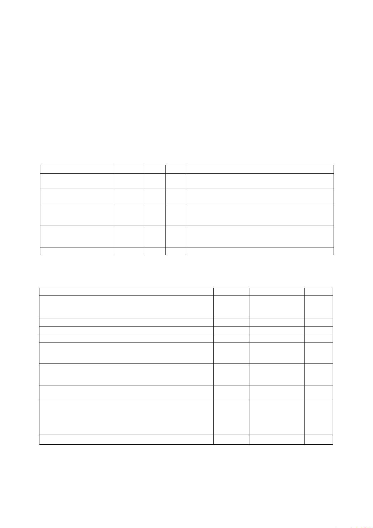
VDE 0884 (06.92) Insulation Characteristics

Description Symbol Characteristic Unit

Installation classification per DIN VDE 0110, Table 1

for rated mains voltage ≤ 300 V rms I-IV
for rated mains voltage ≤ 600 V rms I-III

Climatic Classification 40/100/21
Pollution Degree (DIN VDE 0110, Table 1)* 2
Maximum Working Insulation Voltage V

IORM

848 V peak

Input to Output Test Voltage, Method b** V

PR

1591 V peak

VPR = 1.875 x V

IORM

, Production test with tp = 1 sec,

Partial discharge < 5 pC

Input to Output Test Voltage, Method a** V

PR

1273 V peak

VPR = 1.5 x V

IORM

, Type and sample test with tp = 60 sec,

Partial discharge < 5 pC

Highest Allowable Overvoltage**
(Transient Overvoltage tTR = 10 sec) V

TR

6000 V peak

Safety-limiting values (Maximum values allowed in the event
of a failure, also see Figure 27)

Case Temperature T

S

175 °C

Input Power P

S,Input

80 mW

Output Power P

S,Output

250 mW

Insulation Resistance at TS, VIO = 500 V R

S

≥ 1x10

12

Ω

*This part may also be used in Pollution Degree 3 environments where the rated mains voltage is ≤ 300 V rms (per DIN VDE 0110).
**Refer to the front of the optocoupler section of the current catalog for a more detailed description of VDE 0884 and other product
safety requirements.

Note: Optocouplers providing safe electrical separation per VDE 0884 do so only within the safety-limiting values to which they are
qualified. Protective cut-out switches must be used to ensure that the safety limits are not exceeded.

Regulatory Information

The HCPL-7800 has been
approved by the following
organizations:

UL

Recognized under UL 1577,
Component Recognition
Program, File E55361.

CSA

Approved under CSA Component
Acceptance Notice #5, File CA

88324.

Insulation and Safety Related Specifications

Parameter Symbol Value Units Conditions

Min. External Air Gap L(IO1) 7.4 mm Measured from input terminals to output terminals,
(External Clearance) shortest distance through air

Min. External Tracking L(IO2) 8.0 mm Measured from input terminals to output terminals,
Path (External Creepage) shortest distance path along body

Min. Internal Plastic Gap 0.5 mm Through insulation distance, conductor to conductor,
(Internal Clearance) usually the direct distance between the photoemitter

and photodetector inside the optocoupler cavity

Tracking Resistance CTI 175 V DIN IEC 112/VDE 0303 Part 1
(Comparative Tracking
Index)

Isolation Group III a Material Group (DIN VDE 0110, 1/89, Table 1)

Option 300 – surface mount classification is Class A in accordance with CECC 00802.

VDE

Approved according to VDE
0884/06.92.

1-220

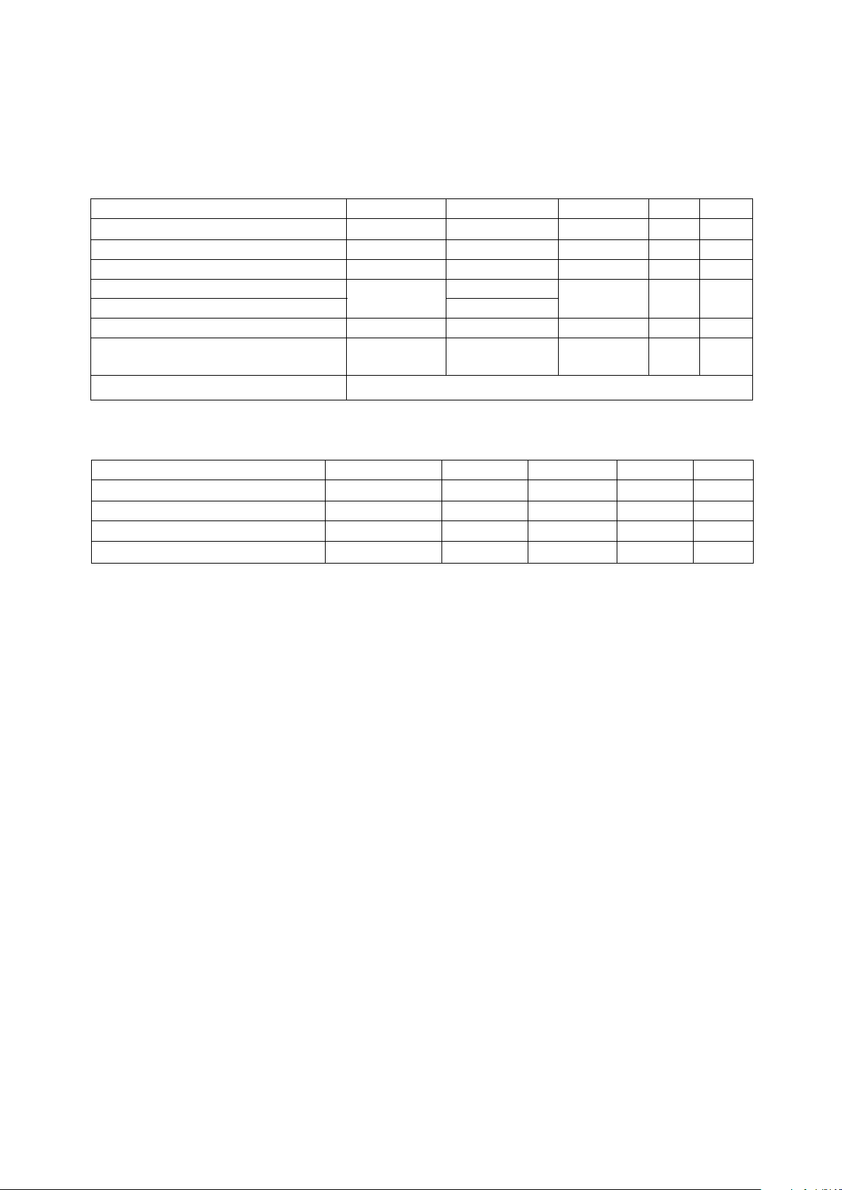
Absolute Maximum Ratings

Parameter Symbol Min. Max. Unit Note

Storage Temperature T

S

-55 125 °C

Ambient Operating Temperature T

A

- 40 100 °C

Supply Voltages V

DD1

, V

DD2

0.0 5.5 V

Steady-State Input Voltage V

IN+

, V

IN-

-2.0 V

DD1

+0.5 V
Two Second Transient Input Voltage -6.0
Output Voltages V

OUT+

, V

OUT-

-0.5 V

DD2

+0.5 V
Lead Solder Temperature T

LS

260 °C1

(1.6 mm below seating plane, 10 sec.)
Reflow Temperature Profile See Package Outline Drawings Section

Recommended Operating Conditions

Parameter Symbol Min. Max. Unit Note

Ambient Operating Temperature T

A

-40 85 °C2

Supply Voltages V

DD1

, V

DD2

4.5 5.5 V 3

Input Voltage V

IN+

, V

IN-

-200 200 mV 4

Output Current |IO|1mA5

1-221

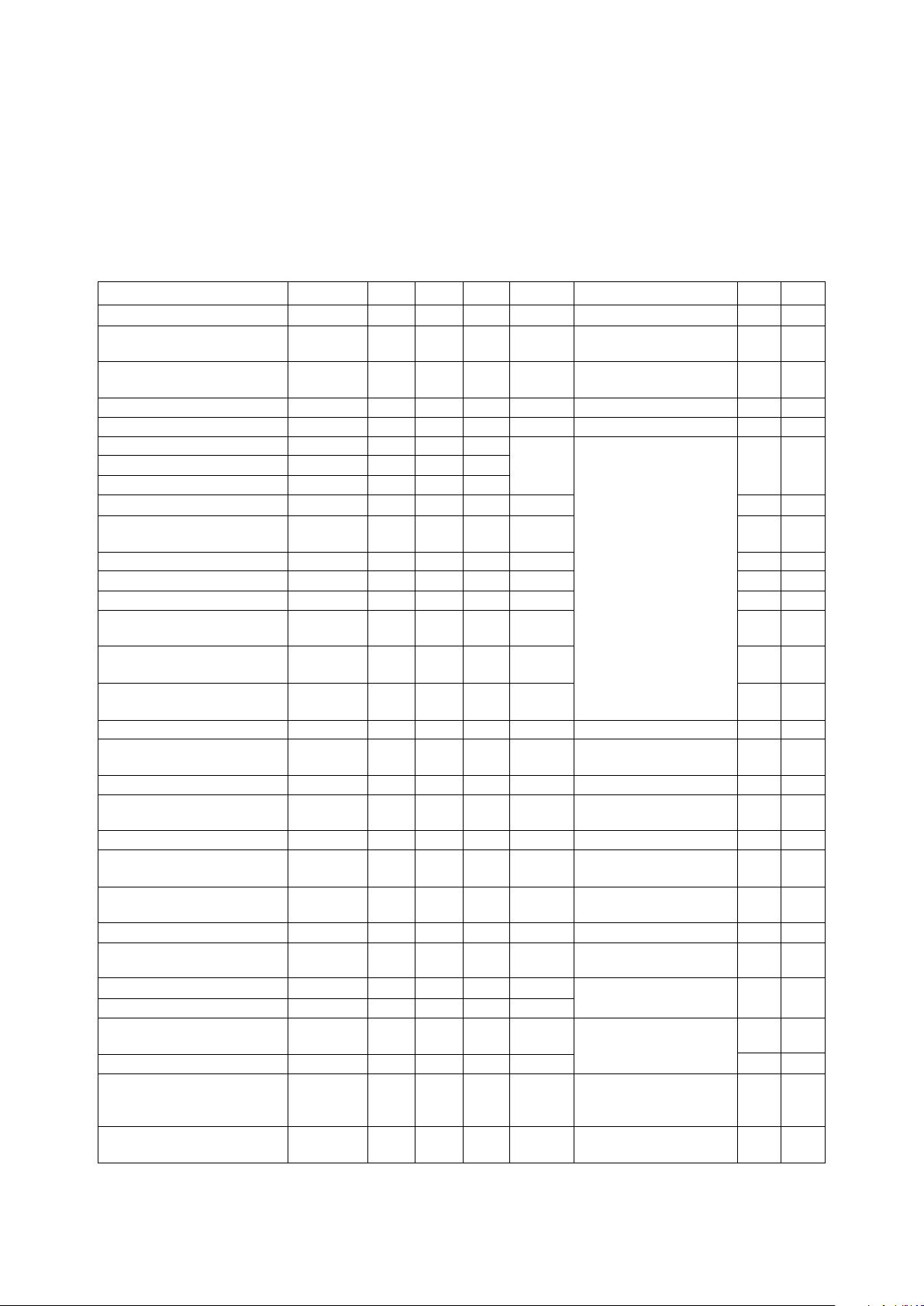
DC Electrical Specifications

All specifications and figures are at the nominal operating condition of V

IN+

= 0 V, V

IN-

= 0 V, TA = 25°C, V

DD1

=

5.0 V, and V

DD2

= 5.0 V, unless otherwise noted.

Parameter Symbol Min. Typ. Max. Unit Test Conditions Fig. Note

Input Offset Voltage V

OS

-1.8 -0.9 0.0 mV 1

Input Offset Drift vs. dVOS/dT -2.1 µV/°C 1, 2 6
Temperature

Abs. Value of Input |dV

OS

/dT| 4.6 µV/°C17

Offset Drift vs. Temperature
Input Offset Drift vs. V

DD1

dVOS/dV

DD1

30 µV/V 1, 3 8

Input Offset Drift vs. V

DD2

dVOS/dV

DD2

-40 µV/V 1, 4 9

Gain (± 5% Tol.) G 7.61 8.00 8.40 -200 mV < V

IN+

< 200 mV 1, 5 10

Gain - A Version (± 1% Tol.) G

A

7.85 7.93 8.01

Gain - B Version (± 1% Tol.) G

B

7.99 8.07 8.15

Gain Drift vs. Temperature dG/dT 0.001 %/°C 5, 6 11
Abs. Value of Gain Drift vs. |dG/dT| 0.001 %/°C512

Temperature
Gain Drift vs. V

DD1

dG/dV

DD1

0.21 %/V 5, 7 13

Gain Drift vs. V

DD2

dG/dV

DD2

-0.06 %/V 5, 8 14

200 mV Nonlinearity NL

200

0.2 0.35 % 5, 9 15

200 mV Nonlinearity Drift dNL

200

/dT -0.001 % pts/°C5, 1016

vs. Temperature
200 mV Nonlinearity Drift dNL

200

/dV

DD1

-0.005 % pts/V 5, 11 17

vs. V

DD1

200 mV Nonlinearity Drift dNL

200

/dV

DD2

-0.007 % pts/V 5, 12 18

vs. V

DD2

100 mV Nonlinearity NL

100

0.1 0.25 % -100 mV< V

IN+

< 100 mV 5, 13 19

Maximum Input Voltage |V

IN+|max

300 mV 14

Before Output Clipping
Average Input Bias Current I

IN

-670 nA 15, 16 20

Input Bias Current dIIN/dT 3 nA/°C
Temperature Coefficient

Average Input Resistance R

IN

530 kΩ 15 20

Input Resistance dRIN/dT 0.38 %/°C
Temperature Coefficient

Input DC Common-Mode CMRR

IN

72 dB 21

Rejection Ratio
Output Resistance R

O

11 Ω 5

Output Resistance dR

O

/dT 0.6 %/°C

Temperature Coefficient
Output Low Voltage V

OL

1.18 V |V

IN+

| = 500 mV 14 22

Output High Voltage V

OH

3.61 V I

OUT+

= 0 A, I

OUT–

= 0 A

Output Common-Mode V

OCM

2.20 2.39 2.60 V -40°C < TA < 85°C14

Voltage 4.5 V < V

DD1

< 5.5 V

Input Supply Current I

DD1

10.7 15.5 mA 17 23

Output Supply Current I

DD2

11.6 14.5 mA V

IN+

= 200 mV, 18 24

-40° C < T

A

< 85°C

4.5 V < V

DD2

< 5.5 V

Output Short-Circuit |I

OSC

| 9.3 mA V

OUT

= 0 V or V

DD2

25

Current

1-222

AC Electrical Specifications

All specifications and figures are at the nominal operating condition of V

IN+

= 0 V, V

IN-

= 0 V, TA = 25° C,

V

DD1

= 5.0 V, and V

DD2

= 5.0 V, unless otherwise noted.

Parameter Symbol Min. Typ. Max. Unit Test Conditions Fig. Note

Rising Edge Isolation IMR

R

10 25 kV/µsVIM = 1 kV 19, 20 26

Mode Rejection
Falling Edge Isolation IMR

F

10 15 kV/µs

Mode Rejection
Isolation Mode Rejection IMRR >140 dB 19 27

Ratio at 60 Hz
Propagation Delay to 10% t

PD10

2.0 3.3 µs -40°C < TA < 85°C 21, 22

Propagation Delay to 50% t

PD50

3.4 5.6 µs

Propagation Delay to 90% t

PD90

6.3 9.9 µs

Rise/Fall Time (10%-90%) t

R/F

4.3 6.6 µs

Bandwidth (-3 dB) f

-3dB

50 85 kHz 23, 24

Bandwidth (-45°)f

-45°

35 kHz

RMS Input-Referred V

N

300 µV rms Bandwidth = 100 kHz 25, 26 28

Noise
Power Supply Rejection PSR 5 mV

p-p

29

Package Characteristics

All specifications and figures are at the nominal operating condition of V

IN+

= 0 V, V

IN-

= 0 V, TA = 25°C, V

DD1

= 5.0 V, and V

DD2

= 5.0 V, unless otherwise noted.

Parameter Symbol Min. Typ. Max. Unit Test Conditions Fig. Note

Input-Output Momentary V

ISO

3750 V rms t = 1 min., RH ≤ 50% 30, 31

Withstand Voltage*
Input-Output Resistance R

I-O

101210

13

Ω TA = 25° CV

I-O

= 500 Vdc 30

10

11

TA = 100°C

Input-Output Capacitance C

I-O

0.7 pF f = 1 MHz 30

Input IC Junction-to- θ

jci

96 °C/W 32

Case Thermal Resistance
Output IC Junction-to-Case θ

jco

114 °C/W

Thermal Resistance

*The Input-Output Momentary Withstand Voltage is a dielectric voltage rating that should not be interpreted as an input-output
continuous voltage rating. For the continuous voltage rating refer to the VDE 0884 Insulation Characteristics Table (if applicable), your
equipment level safety specification, or HP Application Note 1074, “Optocoupler Input-Output Endurance Voltage.”

1-223

Notes:

General Note: Typical values represent the
mean value of all characterization units at
the nominal operating conditions. Typical
drift specifications are determined by
calculating the rate of change of the speci­fied parameter versus the drift parameter
(at nominal operating conditions) for each
characterization unit, and then averaging
the individual unit rates. The correspond­ing drift figures are normalized to the
nominal operating conditions and show
how much drift occurs as the particular
drift parameter is varied from its nominal
value, with all other parameters held at
their nominal operating values. Figures
show the mean drift of all characterization
units as a group, as well as the ± 2-sigma
statistical limits. Note that the typical drift
specifications in the tables below may
differ from the slopes of the mean curves
shown in the corresponding figures.

1. HP recommends the use of non­chlorine activated fluxes.

2. The HCPL-7800 will operate properly
at ambient temperatures up to 100°C
but may not meet published specifi­cations under these conditions.

3. DC performance can be best
maintained by keeping V

DD1

and V

DD2

as close as possible to 5 V. See
application section for circuit
recommendations.

4. HP recommends operation with V

IN-

= 0 V (tied to GND1). Limiting V

IN+

to 100 mV will improve DC
nonlinearity and nonlinearity drift. If
V

IN-

is brought above 800 mV with
respect to GND1, an internal test
mode may be activated. This test mode
is not intended for customer use.

5. Although, statistically, the average
difference in the output resistance of
pins 6 and 7 is near zero, the standard
deviation of the difference is 1.3 Ω
due to normal process variations.
Consequently, keeping the output
current below 1 mA will ensure the
best offset performance.

6. Data sheet value is the average change
in offset voltage versus temperature at
TA=25°C, with all other parameters
held constant. This value is expressed
as the change in offset voltage per °C
change in temperature.

7. Data sheet value is the average
magnitude of the change in offset
voltage versus temperature at
TA=25°C, with all other parameters
held constant. This value is expressed

as the change in magnitude per °C
change in temperature.

8. Data sheet value is the average change
in offset voltage versus input supply
voltage at V

DD1

= 5 V, with all other
parameters held constant. This value
is expressed as the change in offset
voltage per volt change of the input
supply voltage.

9. Data sheet value is the average change
in offset voltage versus output supply
voltage at V

DD2

= 5 V, with all other
parameters held constant. This value
is expressed as the change in offset
voltage per volt change of the output
supply voltage.

10. Gain is defined as the slope of the
best-fit line of differential output
voltage (V

OUT+

- V

OUT-

) versus

differential input voltage (V

IN+

-V

IN-

)

over the specified input range.

11. Data sheet value is the average change
in gain versus temperature at
TA=25°C, with all other parameters
held constant. This value is expressed
as the percentage change in gain per
°C change in temperature.

12. Data sheet value is the average
magnitude of the change in gain
versus temperature at TA=25°C, with
all other parameters held constant.
This value is expressed as the
percentage change in magnitude per
°C change in temperature.

13. Data sheet value is the average change
in gain versus input supply voltage at
V

DD1

= 5 V, with all other parameters
held constant. This value is expressed
as the percentage change in gain per
volt change of the input supply
voltage.

14. Data sheet value is the average change
in gain versus output supply voltage at
V

DD2

= 5 V, with all other parameters
held constant. This value is expressed
as the percentage change in gain per
volt change of the output supply
voltage.

15. Nonlinearity is defined as the maxi­mum deviation of the output voltage
from the best-fit gain line (see Note

10), expressed as a percentage of the
full-scale differential output voltage
range. For example, an input range of
± 200 mV generates a full-scale differ­ential output range of 3.2 V (± 1.6 V);
a maximum output deviation of 6.4
mV would therefore correspond to a
nonlinearity of 0.2%.

16. Data sheet value is the average change
in nonlinearity versus temperature at
TA=25°C, with all other parameters
held constant. This value is expressed
as the number of percentage points
that the nonlinearity will change per
°C change in temperature. For
example, if the temperature is
increased from 25°C to 35°C, the
nonlinearity typically will decrease by

0.01 percentage points (10°C times

-0.001 % pts/°C) from 0.2% to 0.19%.

17. Data sheet value is the average change
in nonlinearity versus input supply
voltage at V

DD1

= 5 V, with all other
parameters held constant. This value
is expressed as the number of
percentage points that the nonlinearity
will change per volt change of the
input supply voltage.

18. Data sheet value is the average change
in nonlinearity versus output supply
voltage at V

DD2

= 5 V, with all other
parameters held constant. This value
is expressed as the number of
percentage points that the nonlinearity
will change per volt change of the
output supply voltage.

19. NL

100

is the nonlinearity specified over

an input voltage range of ± 100 mV.

20. Because of the switched-capacitor
nature of the input sigma-delta
converter, time-averaged values are
shown.

21. This parameter is defined as the ratio
of the differential signal gain (signal
applied differentially between pins 2
and 3) to the common-mode gain
(input pins tied together and the signal
applied to both inputs at the same
time), expressed in dB.

22. When the differential input signal
exceeds approximately 300 mV, the
outputs will limit at the typical values
shown.

23. The maximum specified input supply
current occurs when the differential
input voltage (V

IN+

- V

IN-

) = 0 V. The
input supply current decreases
approximately 1.3 mA per 1 V
decrease in V

DD1

.

24. The maximum specified output supply
current occurs when the differential
input voltage (V

IN+ -VIN-

) = 200 mV,
the maximum recommended operating
input voltage. However, the output
supply current will continue to rise for
differential input voltages up to
approximately 300 mV, beyond which
the output supply current remains
constant.

1-224

Figure 1. Input Offset Voltage Test Circuit. Figure 2. Input-Referred Offset Drift

vs. Temperature.

25. Short circuit current is the amount of
output current generated when either
output is shorted to V

DD2

or ground.

26. IMR (also known as CMR or Common
Mode Rejection) specifies the mini­mum rate of rise of an isolation mode
noise signal at which small output
perturbations begin to appear. These
output perturbations can occur with
both the rising and falling edges of the
isolation-mode wave form and may be
of either polarity. When the perturba­tions first appear, they occur only
occasionally and with relatively small
peak amplitudes (typically 20-30 mV
at the output of the recommended
application circuit). As the magnitude
of the isolation mode transients
increase, the regularity and amplitude
of the perturbations also increase. See
applications section for more
information.

27. IMRR is defined as the ratio of
differential signal gain (signal applied
differentially between pins 2 and 3) to

the isolation mode gain (input pins
tied to pin 4 and the signal applied
between the input and the output of
the isolation amplifier) at 60 Hz,
expressed in dB.

28. Output noise comes from two primary
sources: chopper noise and sigma­delta quantization noise. Chopper
noise results from chopper stabiliza­tion of the output op-amps. It occurs
at a specific frequency (typically 200
kHz at room temperature), and is not
attenuated by the internal output filter.
A filter circuit can be easily added to
the external post-amplifier to reduce
the total rms output noise. The
internal output filter does eliminate
most, but not all, of the sigma-delta
quantization noise. The magnitude of
the output quantization noise is very
small at lower frequencies (below 10
kHz) and increases with increasing
frequency. See applications section for
more information.

29. Data sheet value is the differential
amplitude of the transient at the
output of the HCPL-7800 when a
1V

pk-pk

, 1 MHz square wave with 5 ns
rise and fall times is applied to both
V

DD1

and V

DD2

.

30. This is a two-terminal measurement:
pins 1-4 are shorted together and pins
5-8 are shorted together.

31. In accordance with UL1577, for
devices with minimum V

ISO

specified at

3750 V

rms

, each optocoupler is proof­tested by applying an insulation test
voltage greater-than-or-equal-to 4500
V

rms

for one second (leak current

detection limit, I

I-O

<5µA). This test

is performed before the method b,
100% production test for partial
discharge shown in the VDE 0884
Insulation Characteristics Table.

32. Case temperature was measured with a
thermocouple located in the center of
the underside of the package.

1
2
3
4

8

7
6

5

HCPL-7800

+5 V+5 V +15 V

0.1 µF 0.1 µF

0.1 µF

0.1 µF

0.33 µF0.33 µF

10 K

10 K

-15 V

AD624CD
GAIN = 1000

+

-

V

OUT

1000

500

0

-500

-40 -20 0 20 40 60 80

100

1500

-1000

T – TEMPERATURE – °C

A

dV – INPUT-REFERRED OFFSET DRIFT – µV

OS

MEAN
± 2 SIGMA

1-225

Figure 3. Input-Referred Offset Drift
vs. V

DD1

(V

DD2

= 5 V).

Figure 4. Input-Referred Offset Drift
vs. V

DD2

(V

DD1

= 5 V).

Figure 5. Gain and Nonlinearity Test Circuit. Figure 6. Gain Drift vs. Temperature.

Figure 7. Gain Drift vs.
V

DD1

(V

DD2

= 5 V).

Figure 8. Gain Drift vs.
V

DD2

(V

DD1

= 5 V).

Figure 9. 200 mV Nonlinearity Error
Plot.

400

200

0

-200

4.4 4.6 4.8 5.0 5.2 5.4 5.6

600

-600

V – INPUT SUPPLY VOLTAGE – V

DD1

dV – INPUT-REFERRED OFFSET DRIFT – µV

OS

-400

MEAN
± 2 SIGMA

300

200

100

0

4.4 4.6 4.8 5.0 5.2 5.4 5.6

400

-200

V – OUTPUT SUPPLY VOLTAGE – V

DD2

dV – INPUT-REFERRED OFFSET DRIFT – µV

OS

-100

MEAN
± 2 SIGMA

1

2
3
4

8

7
6

5

HCPL-7800

+5 V+5 V +15 V

0.1 µF 0.1 µF

0.1 µF

0.1 µF

0.33 µF0.33 µF

10 K

10 K

-15 V

AD624CD
GAIN = 1

+

-

V

OUT

0.01 µF

V

IN

1.5

1.0

0.5

0

-40 -20 0 20 40 60 80

-1.0

T – TEMPERATURE – °C

A

dG – GAIN DRIFT– %

-0.5

MEAN
± 2 SIGMA

100

0.5

0

-0.5

-1.0

4.4 4.6 4.8 5.0 5.2 5.4 5.6

-2.0

V – INPUT SUPPLY VOLTAGE – V

DD1

-1.5

dG – GAIN DRIFT– %

MEAN
± 2 SIGMA

0.5

0.4

0.3

0.2

4.4 4.6 4.8 5.0 5.2 5.4 5.6

0

V – OUTPUT SUPPLY VOLTAGE – V

DD2

0.1

dG – GAIN DRIFT– %

MEAN
± 2 SIGMA

-0.1

0.3

0.2

0.1

0

-0.2 -0.1 0 0.1 0.2

-0.2

V – INPUT VOLTAGE – V

IN

-0.1

ERROR – % OF FULL-SCALE

-0.3

MEAN
± 2 SIGMA

1-226

Figure 10. 200 mV Nonlinearity Drift
vs. Temperature.

Figure 11. 200 mV Nonlinearity Drift
vs. V

DD1

(V

DD2

= 5 V).

Figure 12. 200 mV Nonlinearity Drift
vs. V

DD2

(V

DD1

= 5 V).

Figure 18. Typical Output Supply
Current vs. Input Voltage.

Figure 16. Typical Input Current vs.
Input Voltage.

Figure 17. Typical Input Supply
Current vs. Input Voltage.

Figure 13. 100 mV Nonlinearity Error
Plot.

Figure 14. Typical Output Voltages vs.
Input Voltage.

Figure 15. Typical Input Current vs.
Input Voltage.

0.10

0.05

0

-0.05

-40 -20 0 20 40 60 80 100

0.15

-0.10

T – TEMPERATURE – °C

A

dNL – 200 mV NON-LINEARITY DRIFT – % PTS

200

MEAN
± 2 SIGMA

0.04

0.02

0

-0.02

4.6 4.8 5.0 5.2 5.4 5.6

0.06

-0.04

V – INPUT SUPPLY VOLTAGE – V

DD1

-0.06

MEAN
± 2 SIGMA

4.4

dNL – 200 mV NON-LINEARITY DRIFT – % PTS

200

0.04

0.02

0

-0.02

4.6 4.8 5.0 5.2 5.4 5.6

0.06

-0.04

V – OUTPUT SUPPLY VOLTAGE – V

DD2

MEAN
± 2 SIGMA

4.4

dNL – 200 mV NON-LINEARITY DRIFT – % PTS

200

0.05

0

-0.05

-0.10

-0.05 0 0.05 0.10

0.10

-0.15

V – INPUT VOLTAGE – V

IN

ERROR – % OF FULL-SCALE

-0.10

-0.20

MEAN
± 2 SIGMA

0.15

3.0

2.5

2.0

1.5

-0.4 -0.2 0 0.2

3.5

1.0

V – INPUT VOLTAGE – V

IN

-0.6

4.0

V – OUTPUT VOLTAGE – V

O

0.4 0.6

POSITIVE
OUTPUT
(PIN 7)

NEGATIVE 
OUTPUT
(PIN 6)

-400

-600

-800

-1000

-0.1 0 0.1 0.2

-200

-1200

V – INPUT VOLTAGE – V

IN

-0.2

0

I – INPUT CURRENT – nA

IN

-2

-4

-6

-8

-2 0 2 4

0

-10

V – INPUT VOLTAGE – V

IN

-4

2

I – INPUT CURRENT – mA

IN

-6 6

9.5

9.0

8.5

-0.1 0 0.1 0.2

10.0

V – INPUT VOLTAGE – V

IN

-0.2

10.5

I – INPUT SUPPLY CURRENT – mA

DD1

-0.3 0.3-0.4 0.4

T = -40°C
T = 25°C
T = 85°C

A
A
A

10.5

10.0

12.0

-0.1 0 0.1 0.2

11.0

V – INPUT VOLTAGE – V

IN

-0.2

11.5

I – OUTPUT SUPPLY CURRENT – mA

DD2

-0.3 0.3-0.4 0.4

T = 85°C
T = 25°C
T = -40°C

A
A
A

1-227

Figure 19. Isolation Mode Rejection Test Circuit.

Figure 20. Typical IMR Failure Waveform. Figure 21. Typical Propagation Delays

and Rise/Fall Time vs. Temperature.

1000 V

0 V

V

V

50 mV PERTURBATION
(DEFINITION OF FAILURE)

0 V

IM

O

1
2
3
4

8

7
6

5

HCPL-7800

+5 V

78L05

+15 V

0.1 µF

0.1 µF

0.1 µF

0.1 µF

5.11 K

330 pF

1.00 K

1.00 K

-15 V

OP-42

+

­V

OUT

0.1 µF

IN OUT

9 V

V

IM

PULSE GEN.

5.11 K

330 pF

+

-

4

2

10

20 40 60 80

6

T – TEMPERATURE – °C

A

0

8

t – TIME – µs

-20 100-40

0

DELAY TO 90%
RISE/FALL TIME
DELAY TO 50%
DELAY TO 10%

1-228

Figure 22. Propagation Delay and Rise/Fall Time Test Circuit.

Figure 23. Typical Amplitude and
Phase Response vs. Frequency.

-3

-4

0

5000 10000 50000 100000

-2

f – FREQUENCY – Hz

1000

-1

RELATIVE AMPLITUDE – dB

500100

Ø – PHASE – DEGREES

0

-15

-30

-45

-60

AMPLITUDE
PHASE

-5

-10

Figure 24. Typical 3 dB and 45°
Bandwidths vs. Temperature.

Figure 25. Typical RMS Input-Referred
Noise vs. Input Voltage.

80

70

48

20 40 60 80

90

0

100

-20-40

110

44

40

36

32

T – TEMPERATURE – °C

A

f – 3 dB BANDWIDTH – kHz

-3 dB

f – 45 DEGREE PHASE BANDWIDTH – kHz

-45°

60

28

100

3 dB BANDWIDTH
45 DEGREE PHASE 
BANDWIDTH

1.5

1.0

150 200 250

2.0

100

2.5

500

3.0

V – INPUT VOLTAGE – mV

IN

V – RMS INPUT-REFERRED NOISE – mV

N

0.5

0

NO BANDWIDTH LIMITING
BANDWIDTH LIMITED TO 100 kHz
BANDWIDTH LIMITED TO 10 kHz

1

2
3
4

8

7
6

5

HCPL-7800

+5 V +15 V

0.1 µF

0.1 µF

0.1 µF

10.0 K

2.00 K

2.00 K

-15 V

OP-42

+

­V

OUT

10.0 K

+5 V

0.1 µF

0.01 µF

V

IN

50%

V

OUT

V

IN

90%

50%

10%

t

PD90

t

PD50

t

PD10

t

R/F

1-229

1

2
3
4

8

7
6

5

HCPL-7800

+5 V

+15 V

0.01 µF

C4

0.1 µF

C8

0.1 µF

C7

0.1 µF

R4

10.0 KΩ

C6

75 pF

R1

2.00 KΩ

R2

2.00 KΩ



-15 V

MC34081

+

­V

OUT

C1

0.1 µF

C5

75 pF

+

-

MOTOR

U2

OUT

C2

0.1 µF

HV-

HV+

U3

R

SENSE

R3

10.0 KΩ

FLOATING

POSITIVE

SUPPLY

GATE DRIVE

CIRCUIT

IN

R5

39 Ω

U1

78L05

C3

Applications Information

Functional Description

Figure 28 shows the primary
functional blocks of the HCPL-

7800. In operation, the sigma­delta analog-to-digital converter
converts the analog input signal
into a high-speed serial bit
stream, the time average of which
is directly proportional to the
input signal. This high speed
stream of digital data is encoded
and optically transmitted to the
detector circuit. The detected

signal is decoded and converted
into accurate analog voltage
levels, which are then filtered to
produce the final output signal.

To help maintain device accuracy
over time and temperature,
internal amplifiers are chopper­stabilized. Additionally, the
encoder circuit eliminates the
effects of pulse-width distortion of
the optically transmitted data by
generating one pulse for every
edge (both rising and falling) of

the converter data to be
transmitted, essentially converting
the widths of the sigma-delta
output pulses into the positions
of the encoder output pulses. A
significant benefit of this coding
scheme is that any non-ideal
characteristics of the LED (such
as non-linearity and drift over
time and temperature) have little,
if any, effect on the performance
of the HCPL-7800.

Figure 27. Dependence of Safety­Limiting Parameters on Ambient
Temperature.

Figure 26. Recommended Application Circuit.

P

S

– POWER – mW

0

0

TA – TEMPERATURE – °C

180

400

12040 80 160

100

200

300

OUTPUT POWER, P

S

INPUT POWER, P

S

20 60 100 140

175

1-230

Circuit Information

The recommended application
circuit is shown in Figure 26. A
floating power supply (which in
many applications could be the
same supply that is used to drive
the high-side power transistor) is
regulated to 5 V using a simple
three-terminal voltage regulator.
The input of the HCPL-7800 is
connected directly to the current
sensing resistor. The differential
output of the isolation amplifier is
converted to a ground-referenced
single-ended output voltage with a
simple differential amplifier
circuit. Although the application
circuit is relatively simple, a few
general recommendations should
be followed to ensure optimal
performance.

As shown in Figure 26, 0.1 µF
bypass capacitors should be
located as close as possible to the
input and output power supply
pins of the HCPL-7800. Notice
that pin 2 (V

IN+

) is bypassed with

a 0.01 µF capacitor to reduce
input offset voltage that can be
caused by the combination of
long input leads and the switched­capacitor nature of the input
circuit.

With pin 3 (V

IN-

) tied directly to
pin 4 (GND1), the power-supply
return line also functions as the
sense line for the negative side of
the current-sensing resistor; this
allows a single twisted pair of
wire to connect the isolation
amplifier to the sense resistor. In
some applications, however,
better performance may be
obtained by connecting pins 2
and 3 (V

IN+

and V

IN-

) directly
across the sense resistor with
twisted pair wire and using a
separate wire for the power
supply return line. Both input
pins should be bypassed with 0.01

exhibit better offset performance
than op-amps with JFET or
MOSFET input stages.

In addition, the op-amp should
also have enough bandwidth and
slew rate so that it does not
adversely affect the response
speed of the overall circuit. The
post-amplifier circuit includes a
pair of capacitors (C5 and C6)
that form a single-pole low-pass
filter; these capacitors allow the
bandwidth of the post-amp to be
adjusted independently of the gain
and are useful for reducing the
output noise from the isolation
amplifier. Many different op-amps
could be used in the circuit,
including: MC34082A (Motorola),
TL032A, TLO52A, and TLC277
(Texas Instruments), LF412A
(National Semiconductor).

The gain-setting resistors in the
post-amp should have a tolerance
of 1% or better to ensure
adequate CMRR and adequate
gain tolerance for the overall
circuit. Resistor networks can be
used that have much better ratio
tolerances than can be achieved
using discrete resistors. A resistor
network also reduces the total
number of components for the
circuit as well as the required
board space.

The current-sensing resistor
should have a relatively low value
of resistance to minimize power
dissipation, a fairly low
inductance to accurately reflect
high-frequency signal compo­nents, and a reasonably tight
tolerance to maintain overall
circuit accuracy. Although
decreasing the value of the sense
resistor decreases power
dissipation, it also decreases the
full-scale input voltage making
iso-amp offset voltage effects
more significant. These two

µF capacitors close to the
isolation amplifier. In either case,
it is recommended that twisted­pair wire be used to connect the
isolation amplifier to the current­sensing resistor to minimize
electro-magnetic interference of
the sense signal.

To obtain optimal CMR perfor­mance, the layout of the printed
circuit board (PCB) should
minimize any stray coupling by
maintaining the maximum
possible distance between the
input and output sides of the
circuit and ensuring that any
ground plane on the PCB does not
pass directly below the HCPL-

7800. An example single-sided
PCB layout for the recommended
application circuit is shown in
Figure 29. The trace pattern is
shown in “X-ray” view as it would
be seen from the top of the PCB;
a mirror image of this layout can
be used to generate a PCB.

An inexpensive 78L05 three­terminal regulator is shown in the
recommended application circuit.
Because the performance of the
isolation amplifier can be affected
by changes in the power supply
voltages, using regulators with
tighter output voltage tolerances
will result in better overall circuit
performance. Many different
regulators that provide tighter
output voltage tolerances than the
78L05 can be used, including:
TL780-05 (Texas Instruments),
LM340LAZ-5.0 and LP2950CZ-

5.0 (National Semiconductor).

The op-amp used in the external
post-amplifier circuit should be of
sufficiently high precision so that
it does not contribute a significant
amount of offset or offset drift
relative to the contribution from
the isolation amplifier. Generally,
op-amps with bipolar input stages

1-231

Figure 28. HCPL-7800 Block Diagram.

Figure 29. PC Board Trace Pattern and Loading Diagram Example.

VOLTAGE

REGULATOR

CLOCK

GENERATOR

Σ∆

MODULATOR

ENCODER

LED DRIVE

CIRCUIT

DETECTOR

CIRCUIT

DECODER

AND D/A

FILTER

ISO-AMP
OUTPUT

VOLTAGE

REGULATOR

ISO-AMP

INPUT

ISOLATION

BOUNDARY

conflicting considerations,
therefore, must be weighed
against each other in selecting an
appropriate sense resistor for a
particular application. To
maintain circuit accuracy, it is
recommended that the sense
resistor and the isolation amplifier
circuit be located as close as
possible to one another. Although
it is possible to buy current­sensing resistors from established
vendors (e.g., the LVR-1, -3 and

-5 resistors from Dale), it is also
possible to make a sense resistor
using a short piece of wire or
even a trace on a PC board.

Figures 30 and 31 illustrate the
response of the overall isolation
amplifier circuit shown in Figure

26. Figure 30 shows the response
of the circuit to a ± 200 mV 20
kHz sine wave input and Figure
31 the response of the circuit to a
± 200 mV 20 kHz square wave
input. Both figures demonstrate
the fast, well-behaved response of
the HCPL-7800.

Figure 32 shows how quickly the
isolation amplifier recovers from
an overdrive condition generated
by a 2 kHz square wave swinging
between 0 and 500 mV (note that

the time scale is different from
the previous figures). The first
wave form is the output of the
application circuit with the filter
capacitors removed to show the
actual response of the isolation
amplifier. The second wave form
is the response of the same circuit
with the capacitors installed. The
recovery time and overshoot are
relatively independent of the
amplitude and polarity of the
overdrive signal, as well as its
duration.

For more information, refer to
Application Note 1059.

1-232

Figure 30. Application Circuit Sine Wave Response.

Figure 31. Application Circuit Square Wave Response.

Figure 32. Application Circuit Overload Recovery Waveform.