

Page 1

For ClassPad 300
Spreadsheet
Application
Version 2.0
User’s Guide
E
RJA510188-4
http://classpad.net/
Page 2

Using the Spreadsheet Application
The Spreadsheet application provides you with powerful, take-along-anywhere spreadsheet
capabilities on your ClassPad.
20040801
Page 3

Contents
1
Contents
1 Spreadsheet Application Overview .................................................................... 1-1
Starting Up the Spreadsheet Application ....................................................................... 1-1
Spreadsheet Window ..................................................................................................... 1-1
2 Spreadsheet Application Menus and Buttons................................................... 2-1
3 Basic Spreadsheet Window Operations ............................................................ 3-1
About the Cell Cursor ..................................................................................................... 3-1
Controlling Cell Cursor Movement ................................................................................. 3-1
Navigating Around the Spreadsheet Window ................................................................. 3-2
Hiding or Displaying the Scrollbars ................................................................................ 3-4
Selecting Cells ............................................................................................................... 3-5
Using the Cell Viewer Window ....................................................................................... 3-6
4 Editing Cell Contents ........................................................................................... 4-1
Edit Mode Screen ........................................................................................................... 4-1
Entering the Edit Mode ................................................................................................... 4-2
Basic Data Input Steps ................................................................................................... 4-3
Inputting a Formula ........................................................................................................ 4-4
Inputting a Cell Reference .............................................................................................. 4-6
Inputting a Constant ....................................................................................................... 4-8
Using the Fill Sequence Command ................................................................................ 4-8
Cut and Copy ............................................................................................................... 4-10
Paste ............................................................................................................................. 4-11
Specifying Text or Calculation as the Data Type for a Particular Cell .......................... 4-13
Using Drag and Drop to Copy Cell Data within a Spreadsheet .................................... 4-14
Using Drag and Drop to Obtain Spreadsheet Graph Data ........................................... 4-16
5 Using the Spreadsheet Application with the eActivity Application ................. 5-1
Drag and Drop ................................................................................................................ 5-1
6 Using the Action Menu ........................................................................................ 6-1
Spreadsheet [Action] Menu Basics ................................................................................ 6-1
Action Menu Functions ................................................................................................... 6-4
7 Formatting Cells and Data................................................................................... 7-1
Standard (Fractional) and Decimal (Approximate) Modes ............................................. 7-1
Plain Text and Bold Text ................................................................................................. 7-1
Text and Calculation Data Types .................................................................................... 7-1
Text Alignment ................................................................................................................ 7-2
Number Format .............................................................................................................. 7-2
Changing the Width of a Column ................................................................................... 7-3
8Graphing ............................................................................................................... 8-1
Graph Menu ................................................................................................................... 8-1
Graph Window Menus and Toolbar ................................................................................ 8-8
Basic Graphing Steps ................................................................................................... 8-11
Other Graph Window Operations ................................................................................. 8-13
20040801
Page 4

Spreadsheet Application Overview
1-1
1 Spreadsheet Application Overview
This section describes the configuration of the Spreadsheet application window, and
provides basic information about its menus and commands.
Starting Up the Spreadsheet Application
Use the following procedure to start up the Spreadsheet application.
u ClassPad Operation
(1) On the application menu, tap R.
• This starts the Spreadsheet application and displays its window.
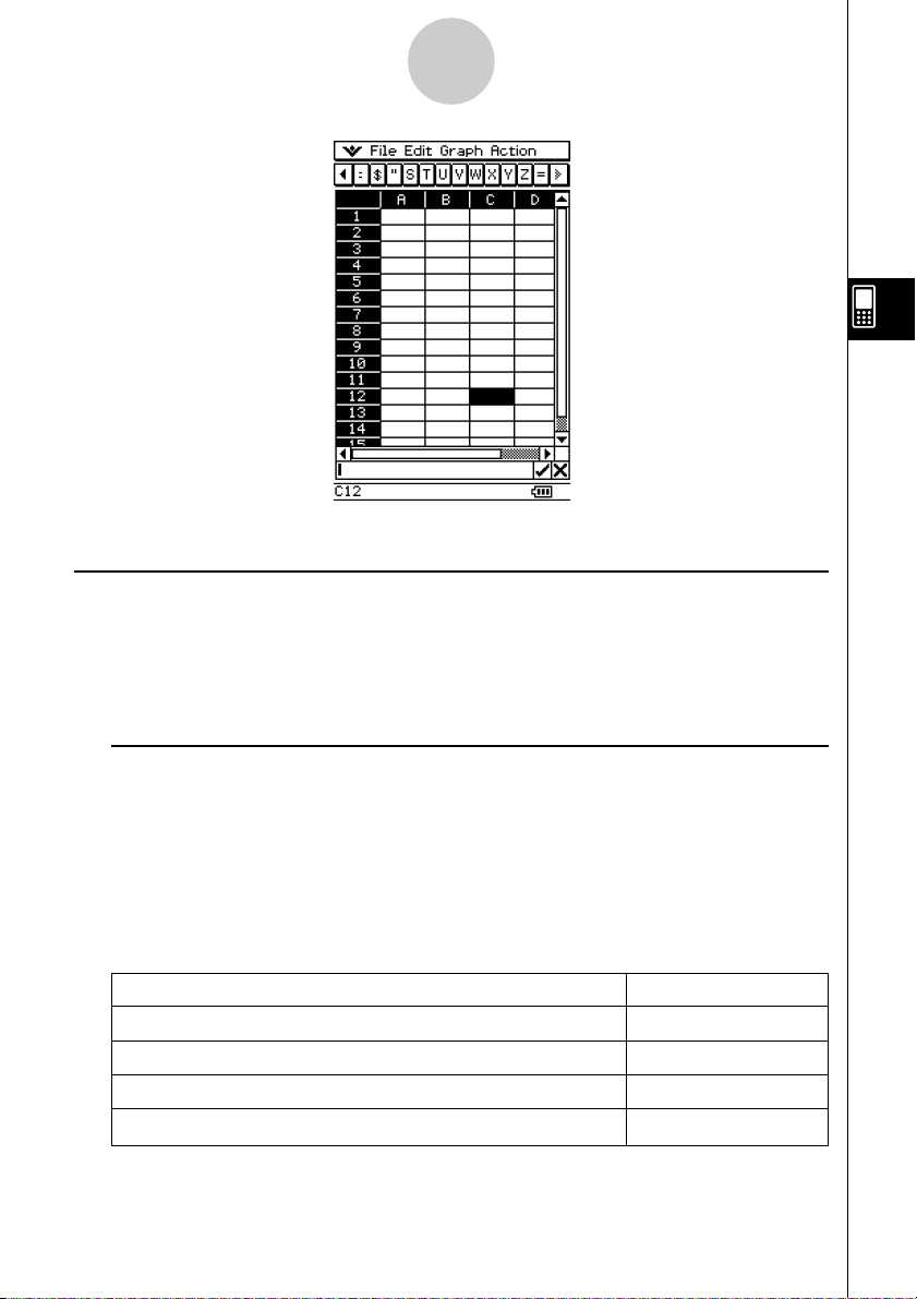
Spreadsheet Window
The Spreadsheet window shows a screen of cells and their contents.
Column letters (A to BL)
Row numbers (1 to 999)
Edit box
Status area
•Each cell can contain a value, expression, text, or a formula. Formulas can contain a
reference to a specific cell or a range of cells.
20040801
Cell cursor
Edit buttons
Page 5
Spreadsheet Application Menus and Buttons
2-1
2 Spreadsheet Application Menus and Buttons
This section explains the operations you can perform using the menus and buttons of the
Spreadsheet application window.
• For information about the O menu, see “Using the O Menu” on page 1-5-4 of your
ClassPad 300 User’s Guide.
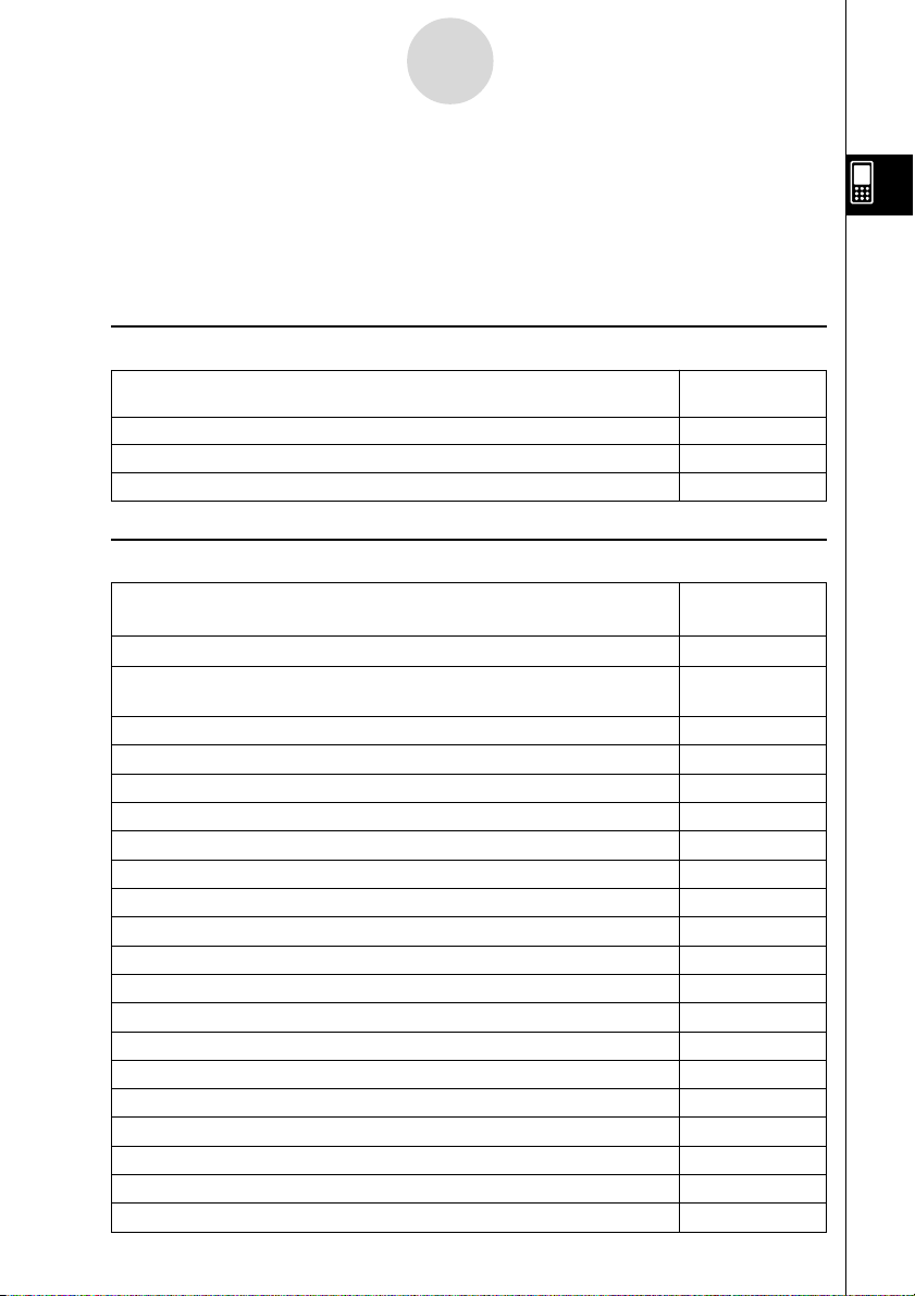
k File Menu
To do this:
Create a new, empty spreadsheet New
Open an existing spreadsheet Open
Save the currently displayed spreadsheet Save
k Edit Menu
To do this:
Undo the last action, or redo the action you have just undone Undo/Redo
Display a dialog box that lets you show or hide scrollbars, and specify the
direction the cursor advances when inputting data
Automatically resize columns to fit the data into the selected cells AutoFit Selection
Display a dialog box for specifying column width Column Width
Display a dialog box for specifying the number format of the selected cell(s)
Display or hide the Cell Viewer window Cell Viewer
Display a dialog box for specifying a cell to jump to Goto Cell
Display a dialog box for specifying a range of cells to select Select Range
Display a dialog box for specifying cell contents and a range of cells to fill
Display a dialog box for specifying a sequence to fill a range of cells Fill Sequence
Insert row(s) Insert - Rows
Insert column(s) Insert - Columns
Delete the currently selected row(s) Delete - Rows
Delete the currently selected column(s) Delete - Columns
Delete the contents of the currently selected cells Delete - Cells
Cut the current selection and place it onto the clipboard Cut
Copy the current selection and place it onto the clipboard Copy
Paste the clipboard contents at the current cell cursor location Paste
Select everything in the spreadsheet Select All
Clear all data from the spreadsheet Clear All
20040801
Select this
[File] menu item:
Select this
[Edit] menu item:
Options
Number Format
Fill Range
Page 6
Spreadsheet Application Menus and Buttons
2-2
k Graph Menu
You can use the [Graph] menu to graph the data contained in selected cells. See “8 Graphing”
for more information.
k Action Menu
The [Action] menu contains a selection of functions that you can use when configuring a
spreadsheet. See “6 Using the Action Menu” for more information.
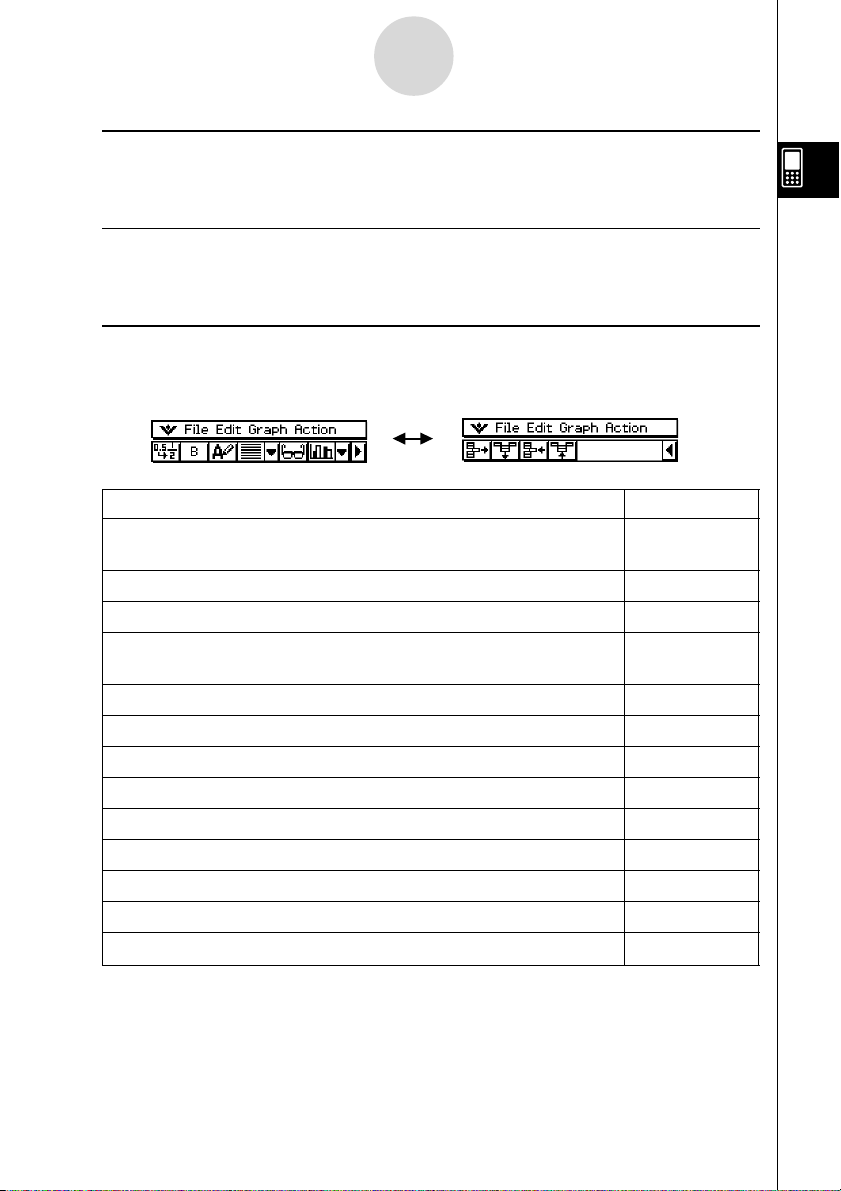
k Spreadsheet Toolbar Buttons
Not all of the Spreadsheet buttons can fit on a single toolbar, tap the u/t button on the far
right to toggle between the two toolbars.
To do this: Tap this button:
Toggle the selected cell(s) between decimal (floating point) and exact
1
display*
Toggle the selected cell(s) between bold and normal M /
Toggle the data type of the selected cell(s) between text and calculation u /
Specify left-justified text and right-justified values for selected cell(s)
(default)
Specify left-justified for selected cell(s) p
Specify centered for selected cell(s) x
Specify right-justified for selected cell(s) ]
Display or hide the Cell Viewer window A
Display the Spreadsheet Graph window (page 8-1) o
Delete the currently selected row(s) H
Delete the currently selected column(s) J
Insert row(s) K
Insert column(s) a
*1 When cell(s) are calculation data types.
.
/
[
,
B
<
Tip
• During cell data input and editing, the toolbar changes to a data input toolbar. See “Edit Mode
Screen” on page 4-1 for more information.
20040801
Page 7
Basic Spreadsheet Window Operations
3-1
3 Basic Spreadsheet Window Operations
This section contains information about how to control the appearance of the Spreadsheet
window, and how to perform other basic operations.
About the Cell Cursor
The cell cursor causes the current selected cell or group of cells to become highlighted. The
location of the current selection is indicated in the status bar, and the value or formula
located in the selected cell is shown in the edit box.
•You can select multiple cells for group formatting, deletion, or insertion.
•See “Selecting Cells” on page 3-5 for more information about selecting cells.
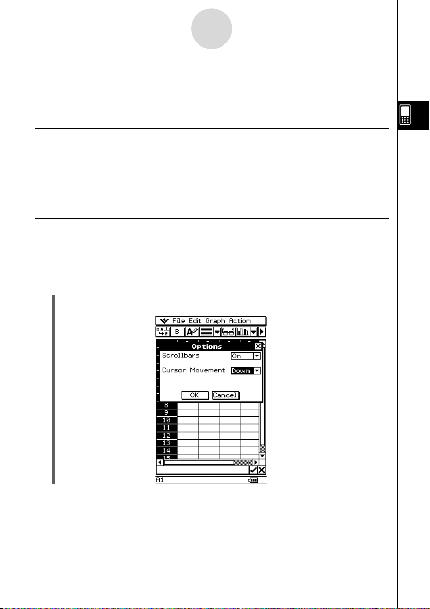
Controlling Cell Cursor Movement
Use the following procedure to specify whether the cell cursor should stay at the current cell,
move down to the next line, or move right to the next column when you register data in a
Spreadsheet cell.
u ClassPad Operation
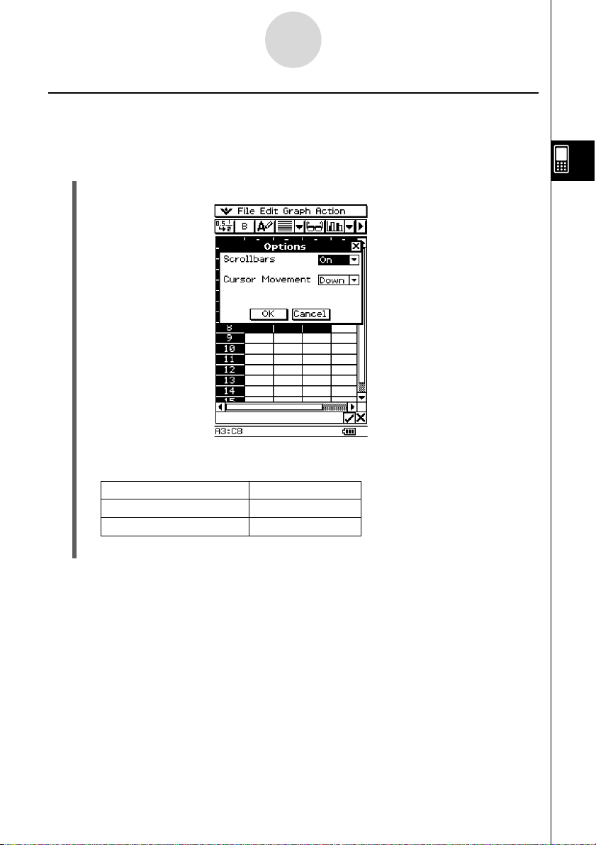
(1) On the [Edit] menu, tap [Options].
20040801
Page 8

Basic Spreadsheet Window Operations
3-2
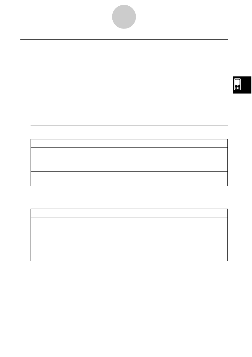
(2) On the dialog box that appears, tap the [Cursor Movement] down arrow button, and
then select the setting you want.
To have the cell cursor behave this way when you register Select this
input: setting:
Remain at the current cell Off
Move to the next row below the current cell Down
Move to the next column to the right of the current cell Right
(3) After the setting is the way you want, tap [OK].
Navigating Around the Spreadsheet Window
The simplest way to select a cell is to tap it with the stylus. You can also drag the stylus
across a range of cells to select all of them. If you drag to the edge of the screen, it will scroll
automatically, until you remove the stylus from the screen.
The following are other ways you can navigate around the Spreadsheet window.
k Cursor Keys
When a single cell is selected, you can use the cursor key to move the cell cursor up, down,
left, or right.
20040801
Page 9
Basic Spreadsheet Window Operations
3-3
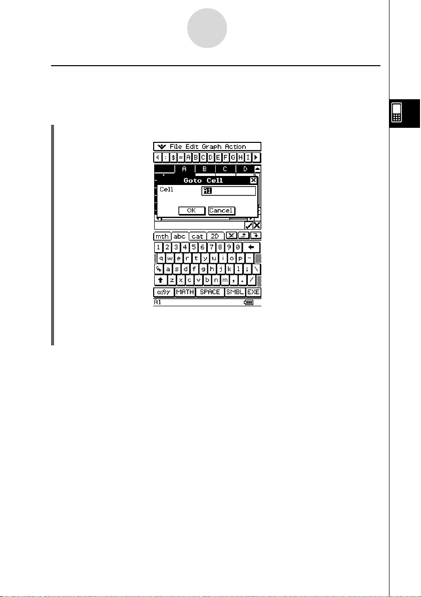
k Jumping to a Cell
You can use the following procedure to jump to a specific cell on the Spreadsheet screen by
specifying the cell’s column and row.
u ClassPad Operation
(1) On the [Edit] menu, select [Goto Cell].
(2) On the dialog box that appears, type in a letter to specify the column of the cell to
which you want to jump, and a value for its row number.
(3) After the column and row are the way you want, tap [OK] to jump to the cell.
20040801
Page 10
Basic Spreadsheet Window Operations
3-4
Hiding or Displaying the Scrollbars
Use the following procedure to turn display of Spreadsheet scrollbars on and off.
By turning off the scrollbars, you make it possible to view more information in the spreadsheet.
u ClassPad Operation
(1) On the [Edit] menu, tap [Options].
(2) On the dialog box that appears, tap the [Scrollbars] down arrow button, and then select
the setting you want.
To do this: Select this setting:
Display the scrollbars On
Hide the scrollbars Off
(3) After the setting is the way you want, tap [OK].
20040801
Page 11
Basic Spreadsheet Window Operations
3-5
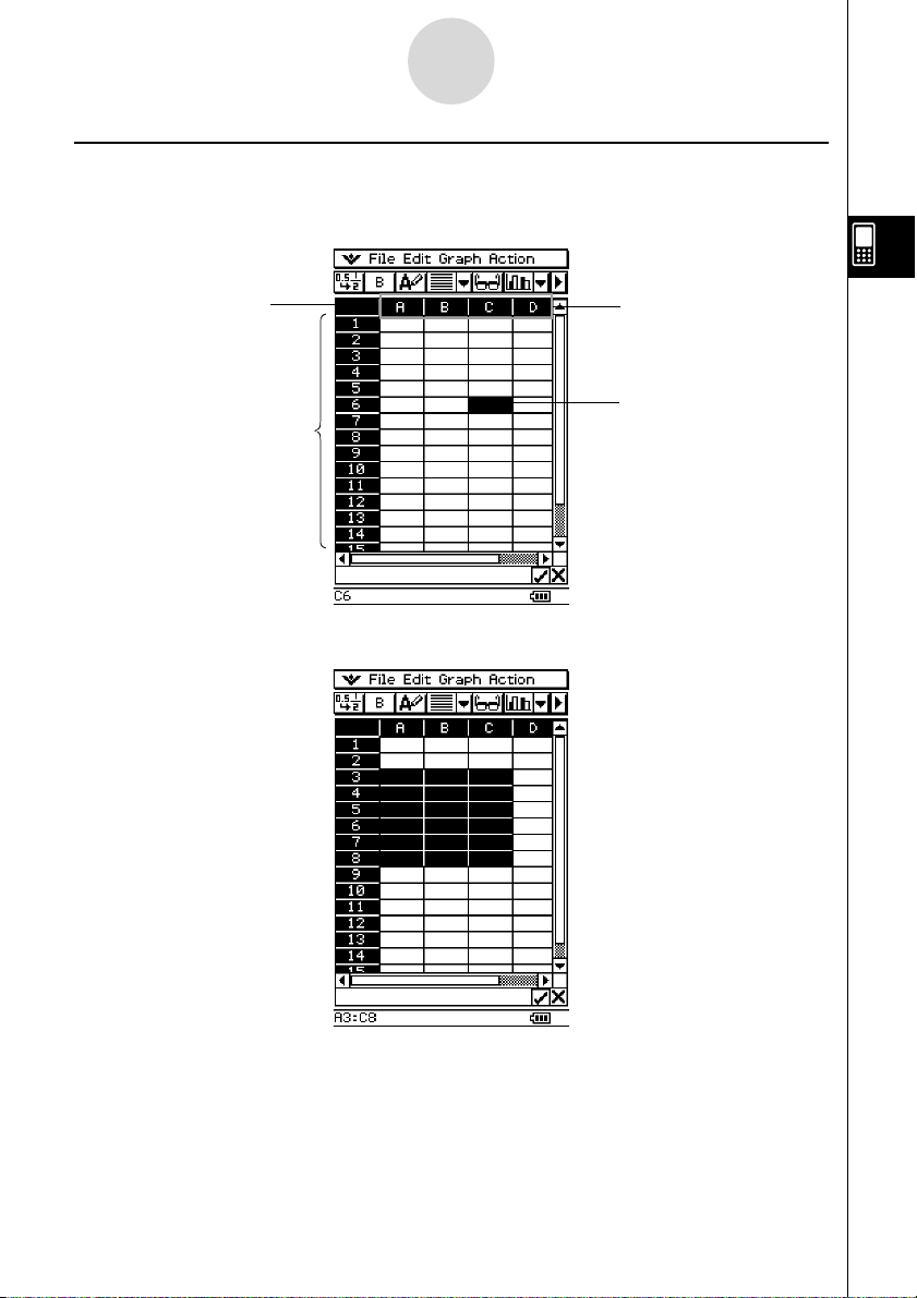
Selecting Cells
Before performing any operation on a cell, you must first select it. You can select a single cell,
a range of cells, all the cells in a row or column, or all of the cells in the spreadsheet.
Tap here to select the
entire spreadsheet.
Tap a row heading to
select the row.
•To select a range of cells, drag the stylus across them.
Tap a column
heading to select
the column.
Tap a cell to select it.
20040801
Page 12
Basic Spreadsheet Window Operations
3-6
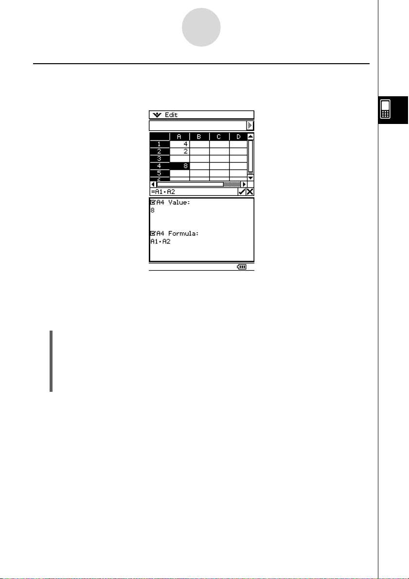
Using the Cell Viewer Window
The Cell Viewer window lets you view both the formula contained in a cell, as well as the
current value produced by the formula.
While the Cell Viewer window is displayed, you can select or clear its check boxes to toggle
display of the value and/or formula on or off. You can also select a value or formula and then
drag it to another cell.
u To view or hide the Cell Viewer window
On the Spreadsheet toolbar, tap A. Or, on the Spreadsheet [Edit] menu, select [Cell
Viewer].
• The above operation toggles display of the Cell Viewer window on and off.
•You can control the size and location of the Cell Viewer window using the r and S
icons on the icon panel below the touch screen. For details about these icons, see “1-3
Using the Icon Panel” of the ClassPad 300 User’s Guide.
20040801
Page 13
Editing Cell Contents
4-1
4 Editing Cell Contents
This section explains how to enter the edit mode for data input and editing, and how to input
various types of data and expressions into cells.
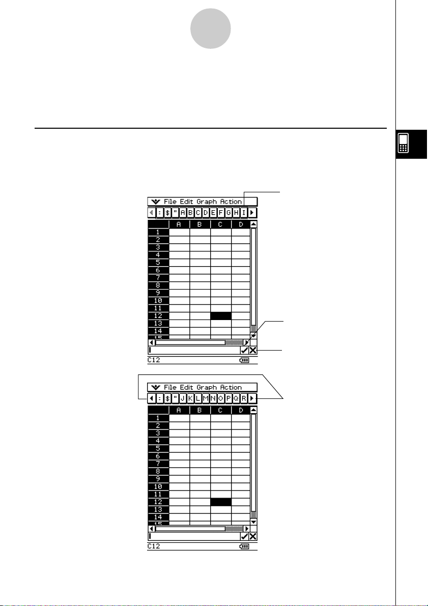
Edit Mode Screen
The Spreadsheet application automatically enters the edit mode whenever you tap a cell to
select it and input something from the keypad.
Entering the edit mode (see page 4-2) displays the editing cursor in the edit box and the data
input toolbar.
Data input toolbar
20040801
Ta p to apply your input
or edits.
Tap to cancel input or
editing without making
any changes.
Tap to scroll the
character buttons.
Page 14
Editing Cell Contents
4-2
•You can tap the data input toolbar buttons to input letters and symbols into the edit box.
Entering the Edit Mode
There are two ways you can enter the edit mode:
•Tapping a cell and then tapping inside the edit box
•Tapping a cell and inputting something on the keypad
The following explains the difference between these two techniques.
k Tapping a cell and then tapping the edit box
• This enters the “standard” edit mode.
•Tapping the edit box selects (highlights) all of the text in the edit box. Tapping the edit box
again deselects (unhighlights) the text and displays the editing cursor (a solid blinking
cursor).
•Be sure to use this standard editing mode when you want to correct or change the existing
contents of a cell.
• The following explains the operation of the cursor key after entering the standard editing
mode.
To move the editing cursor here in the edit box text: Press this cursor key:
One character left d
One character right e
To the beginning (far left) f
To the end (far right) c
20040801
Page 15

Editing Cell Contents
4-3
k Tapping a cell and then inputting something from the keypad
• This enters the “quick” edit mode, indicated by a dashed blinking cursor. Anything you input
with the keypad will be displayed in the edit box.
• If the cell you selected already contains something, anything you input with the quick edit
mode replaces the existing content with the new input.
• In the quick editing mode, pressing the cursor key registers your input and moves the cell
cursor in the direction of the cursor key you press.
•Note that you can change to the standard edit mode at any time during the quick edit mode
by tapping inside of the edit box.
Basic Data Input Steps
The following are the basic steps you need to perform whenever inputting or editing cell
data.
u ClassPad Operation
(1) Enter the edit mode.
• Either tap a cell (quick edit), or tap a cell and then tap the edit box (standard edit).
• See “Selecting Cells” on page 3-5 for more information about selecting cells.
(2) Input the data you want.
•You can input data using the keypad, the [Action] menu, and the input toolbar. See
the following sections for more information.
(3) After you are finished, finalize the input using one of the procedures below.
If you are using this edit mode: Do this to finalize your input:
Standard Edit • Tap the s button next to the edit box.
•Press the E key.
Quick Edit • Press a cursor key.
•Or tap the s button next to the edit box.
•Or press the E key.
• This causes the entire spreadsheet to be re-calculated.
• If you want to cancel data input without saving your changes, tap the S button next to
the edit box or tap on the icon panel.
Important!
•You can also finalize input into a cell by tapping a different cell, as long as the first
character in the edit box is not an equal sign (=). Tapping another cell while the first
character in the edit box is an equal sign (=) inserts a reference to the tapped cell into the
edit box. See “Inputting a Cell Reference” on page 4-6 for more information.
20040801
Page 16
Editing Cell Contents
4-4
Inputting a Formula
A formula is an expression that the Spreadsheet application calculates and evaluates when
you input it, when data related to the formula is changed, etc.
A formula always starts with an equal sign (=), and can contain any one of the following.
•Values
•Mathematical expressions
•Cell references
•ClassPad soft keyboard functions (cat page of keyboard)
•[Action] menu functions (page 6-4)
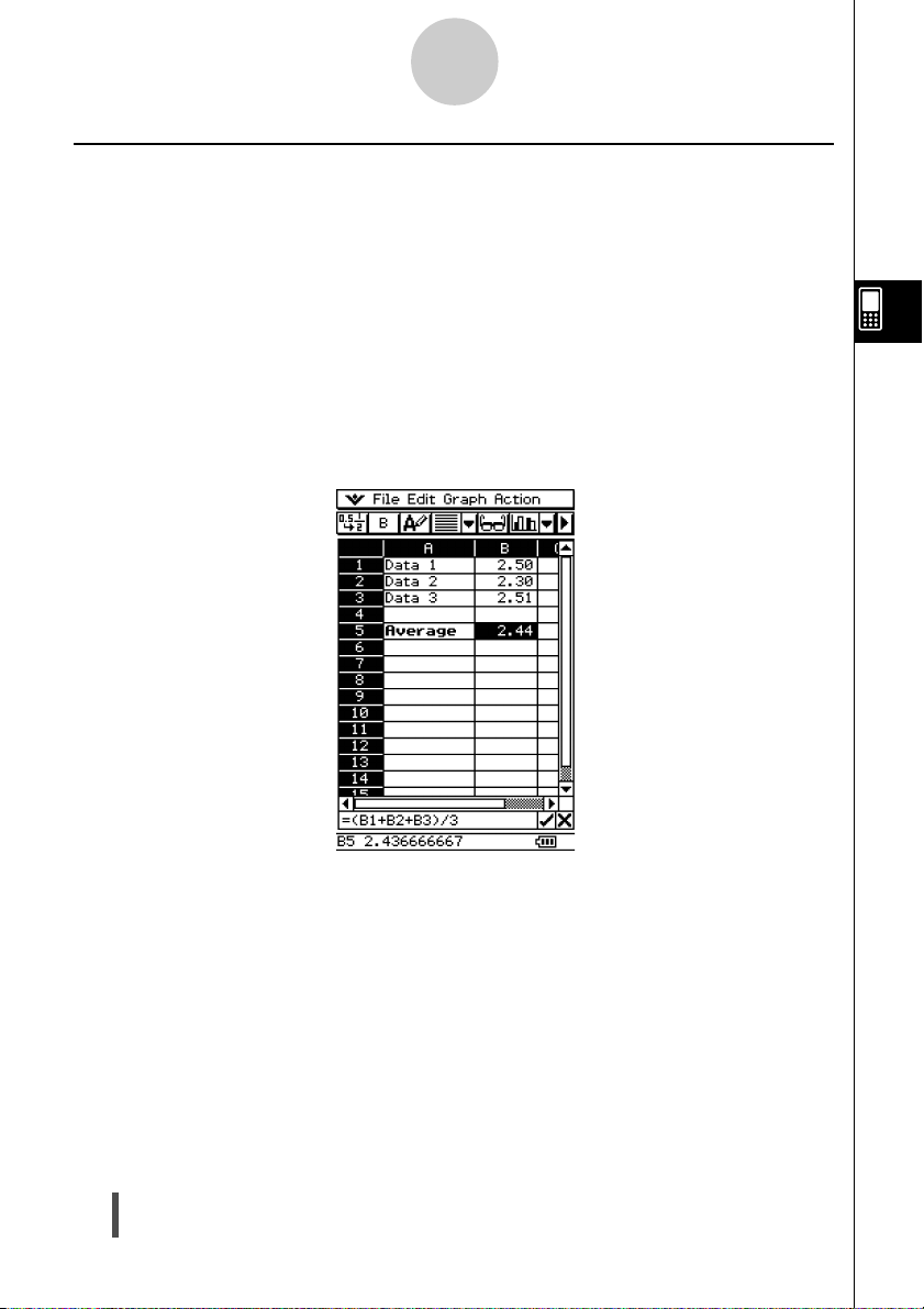
Formulas are calculated dynamically whenever related values are changed, and the latest
result is always displayed in the spreadsheet.
The following shows a simple example where a formula in cell B5 calculates the average of
the values in cells B1 through B3.
Important!
•Tapping another cell while the first character in the edit box is an equal sign (=) inserts a
reference to the tapped cell into the edit box. Dragging across a range of cells will input a
reference to the selected range. See “Inputting a Cell Reference” on page 4-6 for more
information.
•When a cell is set to text data type, formulas are displayed as text when they are not
preceded by an equal sign (=).
•When a cell is set to calculation data type, an error occurs when a formula is not preceded
by an equal sign (=).
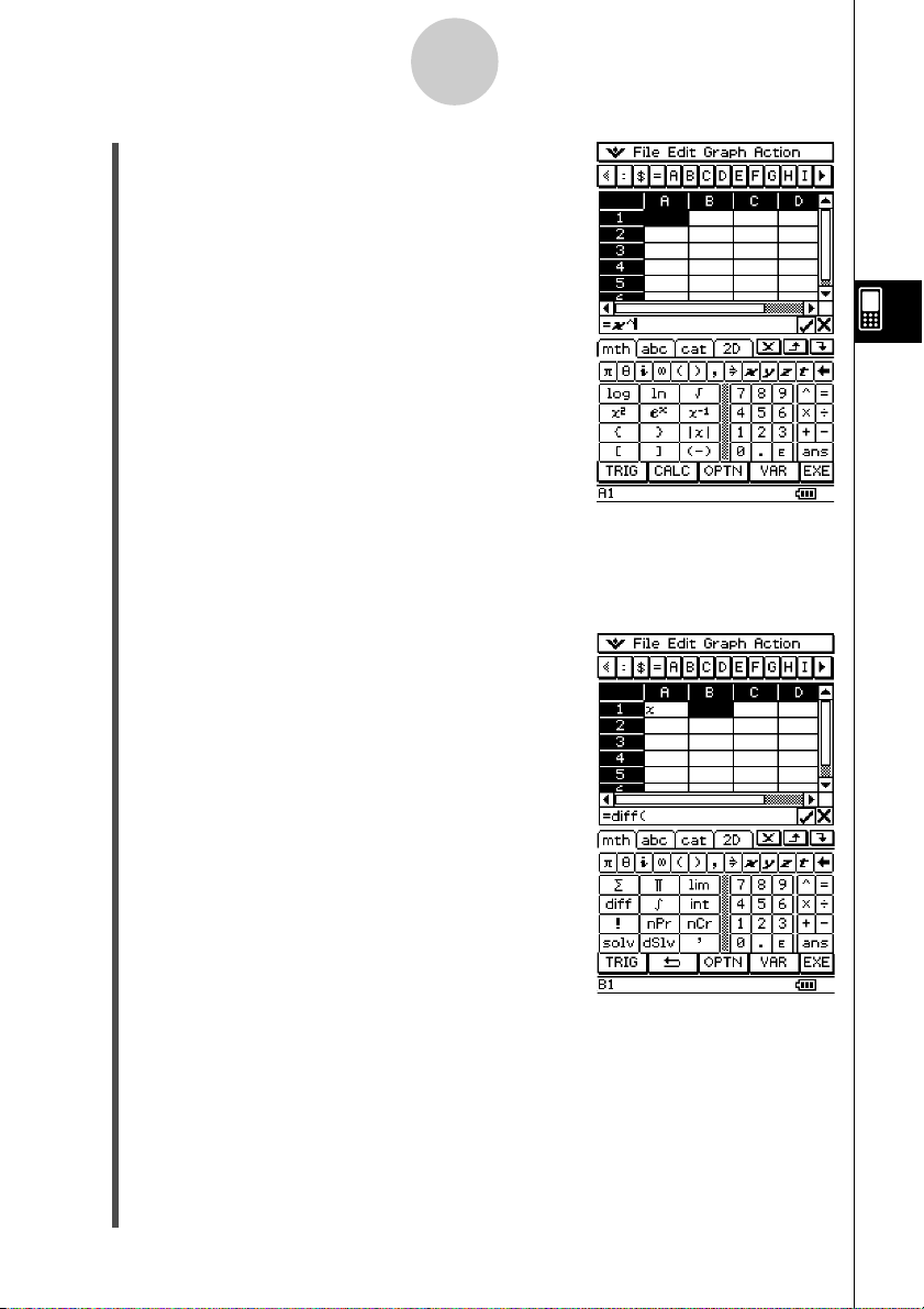
u To use the soft keyboards to input a function
Example: To input the following
(1) Tap cell A1 to select it.
(2) Press =, x, and then {.
Cell A1: x^row(A1)
Cell B1: diff(A1, x, 1)
20040801
Page 17
Editing Cell Contents
4-5
(3) Press k to display the soft keyboard.
(4) Tap the 0 tab and then tap r, o, w, or on the [Action] menu, tap [row].
(5) Press (, tap cell A1, and then press ).
(6) Press E.
(7) Tap cell B1 and then press =.
(8) On the soft keyboard, tap the 9 tab, tap -,
and then tap -.
(9) Tap cell A1, press ,, x, ,, 1, and then press ).
(10) Press E.
(11)Press k to hide the soft keyboard.
(12) Select (highlight) cells A1 and B1.
(13) On the [Edit] menu, tap [Copy].
(14) Select cells A2 and B2.
(15) On the [Edit] menu, tap [Paste].
• Learn more about cell referencing on the next page.
20040801
Page 18
Editing Cell Contents
4-6
Inputting a Cell Reference
A cell reference is a symbol that references the value of one cell for use by another cell. If
you input “=A1 + B1” into cell C2, for example, the Spreadsheet will add the current value of
cell A1 to the current value of cell B1, and display the result in cell C2.
There are two types of cell references:
understand the difference between relative and absolute cell references. Otherwise, your
spreadsheet may not produce the results you expect.
k Relative Cell Reference
A relative cell reference is one that changes according to its location on the spreadsheet.
The cell reference “=A1” in cell C2, for example, is a reference to the cell located “two
columns to the left and one cell up” from the current cell (C2, in this case). Because of this, if
we copy or cut the contents of cell C2 and paste them into cell D12, for example, the cell
reference will change automatically to “=B11”, because B11 is two columns to the left and
one cell up from cell D12.
Be sure to remember that relative cell references always change dynamically in this way
whenever you move them using cut and paste, or drag and drop.
Important!
•When you cut or copy a relative cell reference from the edit box, it is copied to the
clipboard as text and pasted “as-is” without changing. If “=A1” is in cell C2 and you copy
“=A1” from the edit box and paste it into cell D12, for example, D12 will also be “=A1”.
relative
and
absolute
. It is very important that you
k Absolute Cell References
An absolute cell reference is the one that does not change, regardless of where it is located
or where it is copied to or moved to. You can make both the row and column of a cell
reference absolute, or you can make only the row or only the column of a cell reference
absolute, as described below.
This cell reference: Does this:
$A$1 Always refers to column A, row 1
$A1 Always refers to column A, but the row changes dynamically when
A$1 Always refers to row 1, but the column changes dynamically when
Let’s say, for example, that a reference to cell A1 is in cell C1. The following shows what
each of the above cell references would become if the contents of cell C1 were copied to cell
D12.
$A$1 → $A$1
$A1 → $A12
A$1 → B$1
moved, as with a relative cell reference
moved, as with a relative cell reference
20040801
Page 19
Editing Cell Contents
4-7
u To input a cell reference
(1) Select the cell where you want to insert the cell reference.
(2) Tap inside the edit box.
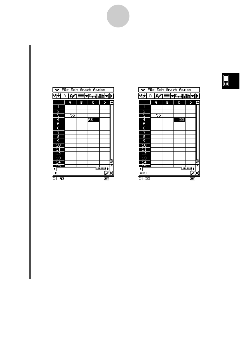
(3) If you are inputting new data, input an equal sign (=) first. If you are editing existing
data, make sure that its first character is an equal sign (=).
• Inputting a cell name like “A3” without an equal sign (=) at the beginning will cause
“A” and “3” to be input as text, without referencing the data in cell A3.
Incorrect cell reference (no “=” sign) Correct cell reference
(4) Tap the cell you want to reference (which will input its name into the edit box
automatically) or use the editing toolbar and keypad to input its name.
Important!
• The above step always inputs a relative cell reference. If you want to input an
absolute cell reference, use the stylus or cursor keys to move the editing cursor to the
appropriate location, and then use the editing toolbar to input a dollar ($) symbol. See
“Inputting a Cell Reference” on page 4-6 for more information about relative and
absolute cell references.
(5) Repeat step (4) as many times as necessary to input all of the cell references you
want. For example, you could input “=A1 + A2”. You can also input a range of cells into
the edit box by dragging across a group of cells.
(6) After your input is the way you want, tap the s button next to the edit box or press the
E key to save it.
20040801
Page 20
Editing Cell Contents
4-8
Inputting a Constant
A constant is data whose value is defined when it is input. When you input something into a
cell for which text is specified as the data type without an equal sign (=) at the beginning, a
numeric value is treated as a constant and non-numeric values are treated as text.
Note the following examples for cells of u type:
This input: Is interpreted as: And is treated as:
sin(1) A numeric expression A constant value
1+1/2 A numeric expression A constant value
1.02389 A numeric expression A constant value
sin(x)A symbolic expression Text
x+y A symbolic expression Text
Result A string expression Text
sin( Invalid expression context Text
•When text is too long to fit in a cell, it spills over into the next cell to the right if the
neighboring cell is empty. If the cell to the right is not empty, the text is cut off and “...” is
displayed to indicate that non-displayed text is contained in the cell.
Using the Fill Sequence Command
The Fill Sequence command lets you set up an expression with a variable, and input a range
of values based on the calculated results of the expression.
u To input a range of values using Fill Sequence
Example: To configure a Fill Sequence operation according to the following parameters
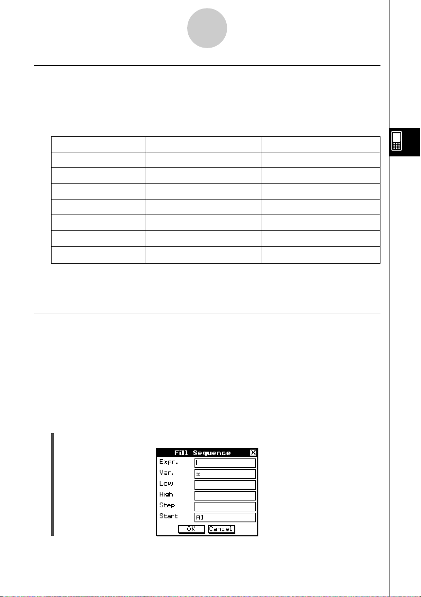
(1) On the [Edit] menu, tap [Fill Sequence].
Expression: 1/x
Change of x Value: From 1 to 25
Step: 1
Input Location: Starting from A1
20040801
Page 21
Editing Cell Contents
4-9
(2) Use the dialog box that appears to configure the Fill Sequence operation as described
below.
Parameter Description
Expr. Input the expression whose results you want to input.
Var.
Specify the name of the variable whose value will change with each
step.
Low Specify the smallest value to be assigned to the variable.
High Specify the greatest value to be assigned to the variable.
Step
Start
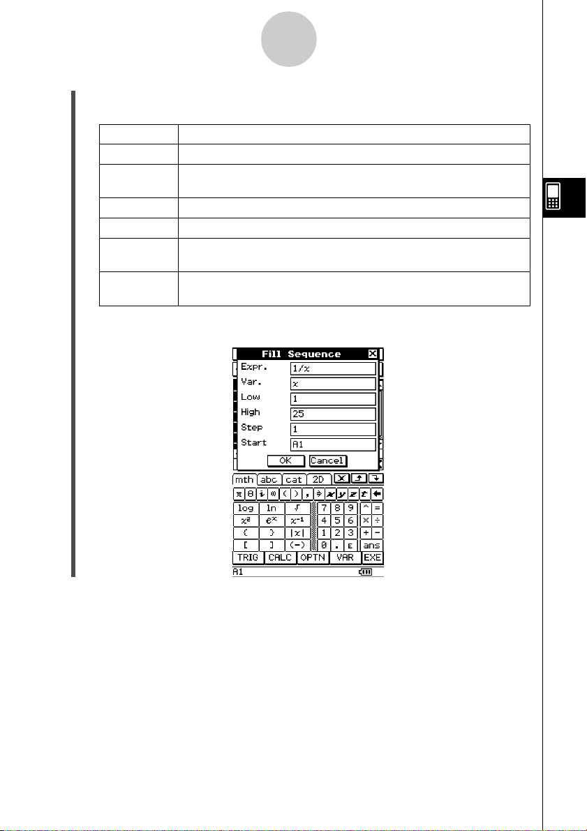
• The following shows how the Fill Sequence dialog box should appear after
Specify the value that should be added to the variable value with
each step.
Specify the starting cell from which the results of the expression
should be inserted.
configuring the parameters for our example.
20040801
Page 22
4-10
Editing Cell Contents
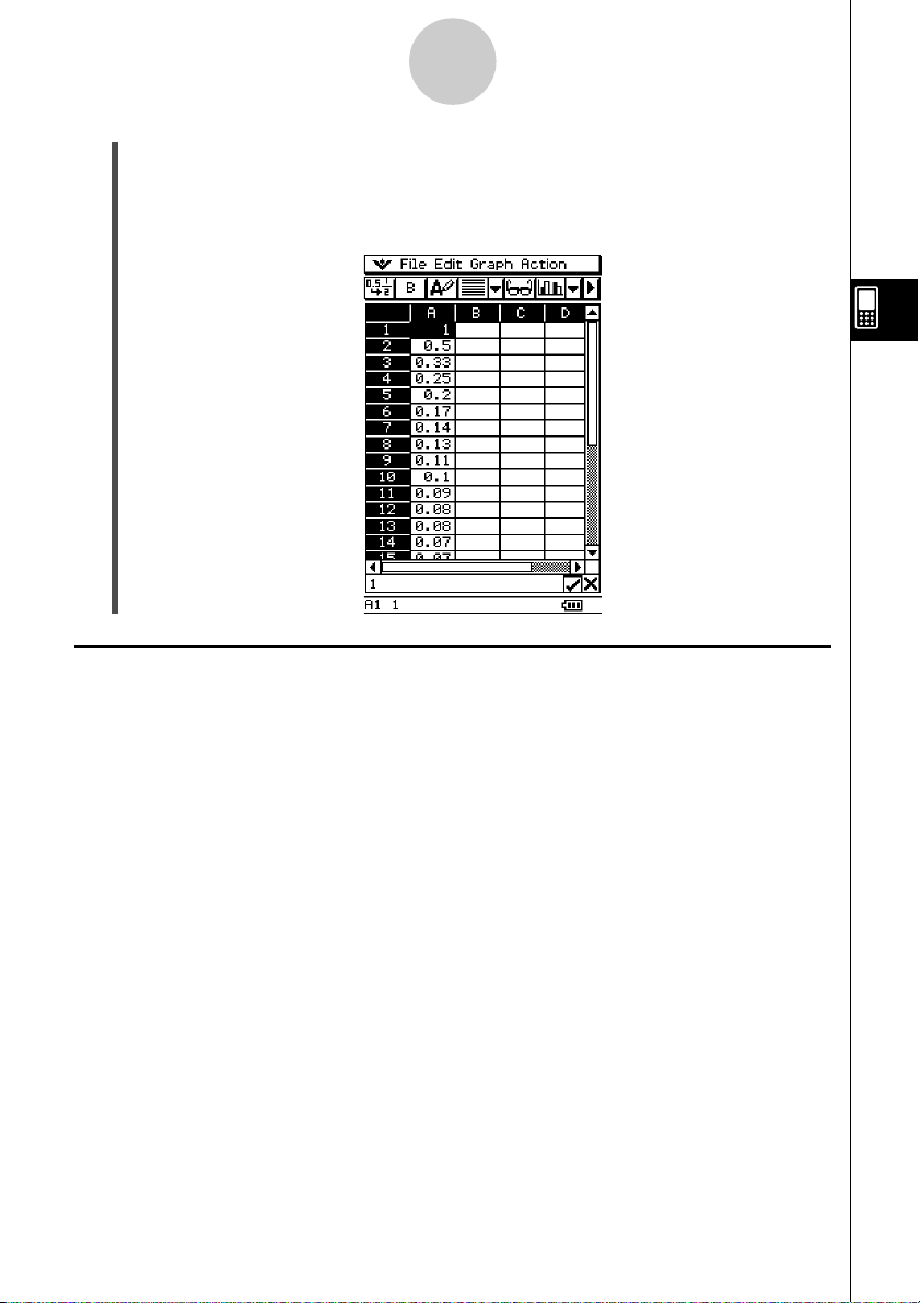
(3) After everything is the way you want, tap [OK].
• This performs all the required calculations according to your settings, and inserts the
results into the spreadsheet.
• The following shows the results for our example.
Cut and Copy
You can use the [Cut] and [Copy] commands on the Spreadsheet application [Edit] menu to
cut and copy the contents of the cells currently selected (highlighted) with the cell cursor. You
can also cut and copy text from the edit box.
The following types of cut/copy operations are supported.
•Single cell cut/copy
•Multiple-cell cut/copy
•Selected edit box text cut/copy
•Cell Viewer values and formulas copy only
Cutting or copying data places it onto the clipboard. You can use the [Paste] command to
paste the clipboard contents at the current cell cursor or editing cursor location.
20040801
Page 23
4-11
Editing Cell Contents
Paste
The [Edit] menu’s [Paste] command lets you paste the data that is currently on the clipboard
at the current cell cursor or editing cursor location.
Important!
•Pasting cell data will cause all relative cell references contained in the pasted data to be
changed in accordance with the paste location. See “Inputting a Cell Reference” on page
4-6 for more information.
•Relative cell references in data copied or cut from the edit box do not change when pasted
into another cell.
The following summarizes how different types of data can be pasted.
k When the clipboard contains data from a single cell or the edit box
If you do this: Executing the [Paste] command will do this:
Select a single cell with the cell cursor Paste the clipboard data into the selected cell
Select multiple cells with the cell cursor Paste the clipboard data into each of the
selected cells
Locate the editing cursor inside the edit Paste the clipboard data at the editing cursor
box location
k When the clipboard contains data from multiple cells
If you do this: Executing the [Paste] command will do this:
Select a single cell with the cell cursor Paste the clipboard data starting from the
Select multiple cells with the cell cursor Paste the clipboard data starting from the first
Locate the editing cursor inside the edit Paste the clipboard data at the editing cursor
box location in matrix format
selected cell
(top left) cell
20040801
Page 24

4-12
Editing Cell Contents
• The following shows how cell data is converted to a matrix format when pasted into the edit
box.
Select the cell where
you want to insert
the text (A6 in this
example), and then
tap inside the edit
box.
Tap [Edit],
and then
[Paste].
To view the matrix
as text, tap the cell
(A6) and then A.
To vi ew the
matrix as
2D, tap u
to change
data types.
20040801
Page 25

4-13
Editing Cell Contents
Specifying Text or Calculation as the Data Type for a Particular Cell
A simple toolbar button operation lets you specify that the data contained in the currently
selected cell or cells should be treated as either text or calculation data. The following shows
how the specified data type affects how a calculation expression is handled when it is input
into a cell.
When this data type is
specified: displayed:
Text u
(toolbar button for text)
Calculation <
(toolbar button for math)
Inputting this into the cell:
=2+2 4
2+2 2+2
=2+2 4
2+2 4
Causes this to be
Important!
•Unless noted otherwise, all of the input examples in this User’s Guide assume that input is
being performed into a cell for which text is specified as the data type. Because of this,
calculations that evaluate will be preceded with an equal sign (=).
u ClassPad Operation
(1) Select the cell(s) whose data type you want to specify.
•See “Selecting Cells” on page 3-5 for information about selecting cells.
(2) On the toolbar, tap the third button from the left (u / <) to toggle the data type
between text and calculation.
20040801
Page 26

4-14
Editing Cell Contents
Using Drag and Drop to Copy Cell Data within a Spreadsheet
You can also copy data from one cell to another within a spreadsheet using drag and drop. If
the destination cell already contains data, it is replaced with the newly dropped data.
•When performing this operation, you can drag and drop between cells, or from one location
to another within the edit box only. You cannot drag and drop between cells and the edit
box.
Important!
•Remember that moving cell data within a spreadsheet using drag and drop will cause all
relative cell references in the data to be changed accordingly. See “Inputting a Cell
Reference” on page 4-6 for more information.
u To drag and drop between cells within a spreadsheet
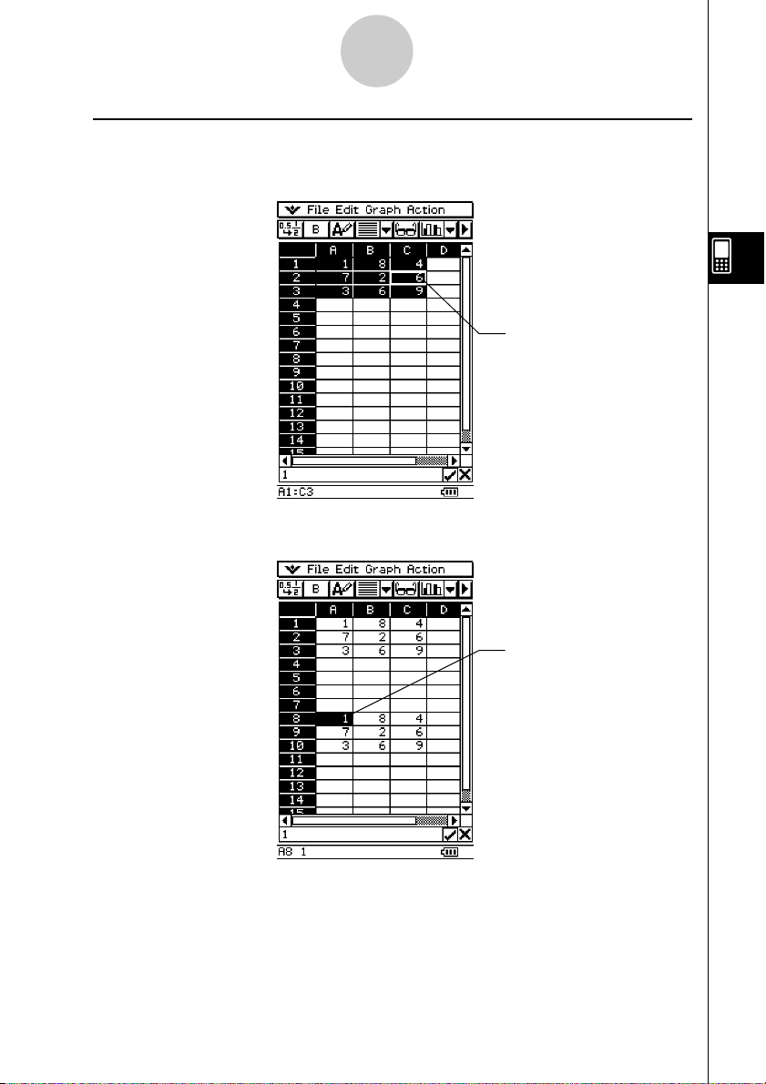
(1) Use the stylus to select the cell or range of cells you want to copy so it is highlighted.
Lift the stylus from the screen after you select the cell(s).
•See “Selecting Cells” on page 3-5 for information about selecting cells.
(2) Hold the stylus against the selected cell(s).
Selection boundary
•Check to make sure that a white selection boundary appears where you hold the
stylus against the screen.
• If you have multiple cells selected (highlighted), the selection boundary will appear
only around the single cell where the stylus is located. See “Dragging and Dropping
Multiple Cells” on page 4-15 for more information.
(3) Drag the stylus to the desired location and then lift the stylus to drop the cell(s) in
place.
20040801
Page 27
4-15
Editing Cell Contents
k Dragging and Dropping Multiple Cells
• When dragging multiple cells, only the cell where the stylus is located has a selection
boundary around it.
Selection boundary
(cursor held against C2)
• When you release the stylus from the screen, the top left cell of the group (originally A1 in
the above example) will be located where you drop the selection boundary.
20040801
Selection boundary
dropped here (A8)
Page 28

4-16
Editing Cell Contents
u To drag and drop within the edit box
(1) Select the cell whose contents you want to edit.
(2) Tap the edit box to enter the edit mode.
(3) Tap the edit box again to display the editing cursor (a solid blinking cursor).
(4) Drag the stylus across the characters you want to move, so they are highlighted.
(5) Holding the stylus against the selected characters, drag to the desired location.
(6) Lift the stylus to drop the characters in place.
Using Drag and Drop to Obtain Spreadsheet Graph Data
The following examples show how you can drag graph data from a Spreadsheet application
Graph window to obtain the graph’s function or the values of the graph’s data.
u To use drag and drop to obtain the function of a graph
Example: To obtain the function of the regression graph shown below
(1) Input data and draw a regression curve.
•See “Other Graph Window Operations” on page 8-13 for more information on
graphing.
(2) Tap the graph window to make it active.
(3) Tap the graph curve and then drag to the cell you want in the Spreadsheet window.
•You can now edit the regression equation in the Spreadsheet edit box and then drag
it back to the Graph window.
• This will cause the graph’s function to appear inside the cell.
20040801
Page 29

4-17
Editing Cell Contents
u To use drag and drop to obtain the data points of a graph
Example: To obtain the data points of the bar graph shown below
(1) Input data and draw a bar graph.
•See “Other Graph Window Operations” on page 8-13 for more information on
graphing.
(2) Tap the Graph window to make it active.
(3) Tap the top of any bar within the Graph window, and then drag to the cell you want in
the Spreadsheet window.
• This will cause the bar graph’s data to appear beginning at the cell you tapped.
20040801
Page 30

Using the Spreadsheet Application with the eActivity Application
5-1
5 Using the Spreadsheet Application with the
eActivity Application
You can display the Spreadsheet application from within the eActivity application. This
makes it possible to drag data between the Spreadsheet and eActivity windows as desired.
Drag and Drop
After you open Spreadsheet within eActivity, you can drag and drop information between the
two application windows.
Example 1: To drag the contents of a single cell from the Spreadsheet window to the
u ClassPad Operation
(1) Tap m to display the application menu, and then tap A to start the eActivity
(2) From the eActivity application menu, tap [Insert] and then [Spreadsheet].
eActivity window
application.
• This inserts a Spreadsheet data strip, and displays the Spreadsheet window in the
lower half of the screen.
Spreadsheet
data strip
Spreadsheet window
• Note that a Spreadsheet data strip works the same way as the Spreadsheet.
(3) Input the text or value you want into the Spreadsheet window.
20040801
Page 31

Using the Spreadsheet Application with the eActivity Application
5-2
(4) Select the cell you want and drag it to the first available line in the eActivity window.
• This inserts the contents of the cell in the eActivity window.
(5) You can now experiment with the data in the eActivity window.
Example 2: To drag a calculation expression from the Spreadsheet edit box to the eActivity
window
u ClassPad Operation
(1) Tap m to display the application menu, and then tap A to start the eActivity
application.
(2) From the eActivity application menu, tap [Insert] and then [Spreadsheet].
• This inserts a Spreadsheet data strip, and displays the Spreadsheet window in the
lower half of the screen.
(3) Select a Spreadsheet cell and input the expression you want.
(4) Tap the edit box to select (highlight) all of the contents of the edit box.
20040801
Page 32

Using the Spreadsheet Application with the eActivity Application
5-3
(5) Drag the contents of the edit box to the first available line in the eActivity window.
• This inserts the contents of the edit box in the eActivity window as a text string.
(6) You can now experiment with the data in the eActivity window.
• The basic operations for the following example are the same for the other examples
described above.
Example 3: Dragging multiple Spreadsheet cells to the eActivity window
20040801
Page 33

Using the Spreadsheet Application with the eActivity Application
5-4
Example 4: Dragging data from eActivity to the Spreadsheet window
20040801
Page 34

Using the Action Menu
6-1
6 Using the Action Menu
Most of the functions that are available from the [Action] menu are similar to those on the
[List-Calculation] sub-menu of the standard [Action] menu.
Spreadsheet [Action] Menu Basics
The following example demonstrates the basic procedure for using functions within the
[Action] menu.
Example: To calculate the sum of the following data, and then to add 100 to it
20040801
Page 35

Using the Action Menu
6-2
uClassPad Operation
(1) With the stylus, tap the cell where you want the result to appear.
• In this example, we would tap cell A1.
(2) On the [Action] menu, tap [sum].
• This inputs an equal sign and the [sum] function into
the edit box.
(3) Use the stylus to drag across the range of data
cells from A7 to C12 to select them.
• “A7:C12” appears to the right of the open parenthesis
of the [sum] function.
20040801
Page 36

Using the Action Menu
6-3
(4) Tap the s button to the right of the edit box.
• This automatically closes the parentheses, calculates
the sum of the values in the selected range, and
displays the result in cell A1.
• You could skip this step and input the closing
parentheses by pressing the ) key on the keypad,
if you want.
(5) Tap the edit box to activate it again, and then tap to the right of the last parenthesis.
(6) Press the + key and then input 100.
(7) Tap the s button to the right of the edit box.
• This calculates the result and displays it in cell A1.
20040801
Page 37

Using the Action Menu
6-4
Action Menu Functions
This section describes how to use each function in the [Action] menu. Please note that start
cell:end cell is equivalent to entering a list.
uu
u min
uu
Function: Returns the lowest value contained in the range of specified cells.
Syntax: min(start cell[:end cell][,start cell[:end cell]] / [,value])
Example: To determine the lowest value in the block whose upper left corner is located at A7
and whose lower right corner is located at C12, and input the result in cell A1:
uu
u max
uu
Function: Returns the greatest value contained in the range of specified cells.
Syntax: max(start cell[:end cell][,start cell[:end cell]] / [,value])
Example: To determine the greatest value in the block whose upper left corner is located at
A7 and whose lower right corner is located at C12, and input the result in cell A1:
20040801
Page 38

Using the Action Menu
6-5
uu
u mean
uu
Function: Returns the mean of the values contained in the range of specified cells.
Syntax: mean(start cell:end cell[,start cell:end cell])
Example: To determine the mean of the values in the block whose upper left corner is
located at A7 and whose lower right corner is located at C12, and input the
result in cell A1:
uu
u median
uu
Function: Returns the median of the values contained in the range of specified cells.
Syntax: median(start cell:end cell[,start cell:end cell])
Example: To determine the median of the values in the block whose upper left corner is
located at A7 and whose lower right corner is located at C12, and input the
result in cell A1:
20040801
Page 39

Using the Action Menu
6-6
uu
u mode
uu
Function: Returns the mode of the values contained in the range of specified cells.
Syntax: mode(start cell:end cell[,start cell:end cell])
Example: To determine the mode of the values in the block whose upper left corner is
located at A7 and whose lower right corner is located at C12, and input the
result in cell A1:
uu
u sum
uu
Function: Returns the sum of the values contained in the range of specified cells.
Syntax: sum(start cell:end cell[,start cell:end cell])
Example: To determine the sum of the values in the block whose upper left corner is
located at A7 and whose lower right corner is located at C12, and input the
result in cell A1:
20040801
Page 40

Using the Action Menu
6-7
uu
u prod
uu
Function: Returns the product of the values contained in the range of specified cells.
Syntax: prod(start cell:end cell[,start cell:end cell])
Example: To determine the product of the values in cells A7 and A8, and input the result in
uu
u cuml
uu
Function: Returns the cumulative sums of the values contained in the range of specified
Syntax: cuml(start cell:end cell)
Example: To determine the cumulative sums of the values in cells B1 through B3, and
cell A1:
cells.
input the result in cell A1:
20040801
Page 41

Using the Action Menu
6-8
uu
u Alist
uu
Function: Returns the differences between values in each of the adjacent cells in the
range of specified cells.
Syntax: Alist(start cell:end cell)
Example: To determine the differences of the values in cells B1 through B3, and input the
result in cell A1:
uu
u stdDev
uu
Function: Returns the sample standard deviation of the values contained in the range of
Syntax: stdDev(start cell:end cell)
Example: To determine the sample standard deviation of the values in the block whose
specified cells.
upper left corner is located at A7 and whose lower right corner is located at C12,
and input the result in cell A1:
20040801
Page 42

Using the Action Menu
6-9
uu
u variance
uu
Function: Returns the sample variance of the values contained in the range of specified
cells.
Syntax: variance(start cell:end cell)
Example: To determine the sample variance of the values in the block whose upper left
corner is located at A7 and whose lower right corner is located at C12, and input
the result in cell A1:
uu
u Q1
uu
Function: Returns the first quartile of the values contained in the range of specified cells.
Syntax: Q1(start cell:end cell[,start cell:end cell])
Example: To determine the first quartile of the values in the block whose upper left corner
is located at A7 and whose lower right corner is located at C12, and input the
result in cell A1:
20040801
Page 43

Using the Action Menu
6-10
uu
u Q3
uu
Function: Returns the third quartile of the values contained in the range of specified cells.
Syntax: Q3(start cell:end cell[,start cell:end cell])
Example: To determine the third quartile of the values in the block whose upper left corner
is located at A7 and whose lower right corner is located at C12, and input the
result in cell A1:
uu
u percent
uu
Function: Returns the percentage of each value in the range of specified cells, the sum of
Syntax: percent(start cell:end cell)
Example: To determine the percentage of the values in cells B1 through B4, and input the
which is 100%.
result in cell A1:
20040801
Page 44

Using the Action Menu
6-11
uu
u polyEval
uu
Function: Returns a polynomial arranged in descending order. The coefficients correspond
sequentially to each value in the range of specified cells.
Syntax: polyEval(start cell:end cell[,start cell:end cell] / [, variable])
Example: To create a second degree polynomial with coefficients that correspond to the
values in cells B1 through B3, and input the result in cell A1:
• “x” is the default variable when you do not specify one above.
• To specify “y” as the variable, for example, enter “=polyEval(B1:B3,y)”.
20040801
Page 45

Using the Action Menu
6-12
uu
u sequence
uu
Function: Returns the lowest-degree polynomial that generates the sequence expressed
by the values in a list or range of specified cells. If we evaluate the polynomial at
2, for example, the result will be the second value in our list.
Syntax: sequence(start cell:end cell[,start cell:end cell][, variable])
Example: To determine a polynomial for the sequence values in cells B1 through B4 and a
variable of “y”, and input the result in cell A1:
• “x” is the default variable when you do not specify one above.
20040801
Page 46

Using the Action Menu
6-13
uu
u sumSeq
uu
Function: Determines the lowest-degree polynomial that generates the sum of the first n
terms of your sequence. If we evaluate the resulting polynomial at 1, for
example, the result will be the first value in your list. If we evaluate the resulting
polynomial at 2, the result will be the sum of the first two values in your list.
When two columns of values or two lists are specified, the resulting polynomial
returns a sum based on a sequence.
Syntax: sumSeq(start cell:end cell[,start cell:end cell][, variable])
Example: To determine a polynomial that generates the sum of the first n terms for the
sequence expressed by the values in cells B1 through B4 with a variable of “y”,
and input the result in cell A1:
• “x” is the default variable when you do not specify one above.
20040801
Page 47

Using the Action Menu
6-14
uu
u row
uu
Function: Returns the row number of a specified cell.
Syntax: row(cell)
Example: To determine the row number of cell A7 and input the result in cell A1:
uu
u col
uu
Function: Returns the column number of a specified cell.
Syntax: col(cell)
Example: To determine the column number of cell C9 and input the result in cell A1:
20040801
Page 48

Using the Action Menu
6-15
uu
u count
uu
Function: Returns a count of the number of cells in the specified range.
Syntax: count(start cell[:end cell])
Example: To count the number of cells in the block whose upper left corner is located at A7
and whose lower right corner is located at C12, and input the result in cell A1:
20040801
Page 49

Formatting Cells and Data
7-1
7 Formatting Cells and Data
This section explains how to control the format of the spreadsheet and the data contained in
the cells.
Standard (Fractional) and Decimal (Approximate) Modes
You can use the following procedure to control whether a specific cell, row, or column, or the
entire spreadsheet should use the standard mode (fractional format) or decimal mode
(approximate value).
u ClassPad Operation
(1) Select the cell(s) whose format you want to specify.
•See “Selecting Cells” on page 3-5 for information about selecting cells.
(2) On the toolbar, tap the left button (, / .) to toggle between the standard mode and
the decimal mode.
Plain Text and Bold Text
Use the following procedure to toggle the text of a specific cell, row, or column, or the entire
spreadsheet between plain and bold.
u ClassPad Operation
(1) Select the cell(s) whose text setting you want to specify.
•See “Selecting Cells” on page 3-5 for information about selecting cells.
(2) On the toolbar, tap the M / B button to toggle between bold and plain text.
Text and Calculation Data Types
Make use of the following procedure to toggle a specific cell, row, or column, or the entire
spreadsheet for either text or calculation data types.
u ClassPad Operation
(1) Select the cell(s) whose format you want to specify.
•See “Selecting Cells” on page 3-5 for information about selecting cells.
(2) On the toolbar, tap the u / < button to toggle between Text Input mode and
Calculation Input mode.
20040801
Page 50

Formatting Cells and Data
7-2
Text Alignment
With the following procedure, you can specify justified, align left, center, or align right for a
specific cell, row, or column, or the entire spreadsheet.
u ClassPad Operation
(1) Select the cell(s) whose alignment setting you want to specify.
•See “Selecting Cells” on page 3-5 for information about selecting cells.
(2) On the toolbar, tap the down arrow button next to the [ button.
(3) On the button menu that appears, tap the text alignment option you want to use.
For this type of alignment: Tap this option:
Left and right justified [
Left p
Center x
Right ]
Number Format
Use the following procedure to specify the number format (Normal 1, Normal 2, Fix 0 – 9,
Sci 0 – 9) of a specific cell, row, or column, or the entire spreadsheet.
u ClassPad Operation
(1) Select the cell(s) whose number format setting you want to specify.
•See “Selecting Cells” on page 3-5 for information about selecting cells.
(2) On the [Edit] menu, tap [Number Format].
(3) On the dialog box that appears, select the number format you want to use.
(4) Tap [OK].
20040801
Page 51

Formatting Cells and Data
7-3
Changing the Width of a Column
There are three different methods you can use to control the width of a column: dragging
with the stylus, using the [Column Width] command, or using the [AutoFit Selection]
command.
u To change the width of a column using the stylus
Use the stylus to drag the edge of a column header left or right until it is the desired width.
u To change the width of a column using the Column Width command
(1) Tap any cell in the column whose width you want to change.
•You could also drag the stylus to select multiple columns, if you want.
(2) On the [Edit] menu, tap [Column Width].
20040801
Page 52

Formatting Cells and Data
7-4
(3) On the dialog box that appears, enter a value in the [Width] box to specify the desired
width of the column in pixels.
•You can also use the [Range] box to specify a different column from the one you
selected in step (1) above, or a range of columns. Entering B1:D1 in the [Range] box,
for example, will change columns B, C, and D to the width you specify.
(4) After everything is the way you want, tap [OK] to change the column width.
u To change the width of a column using the AutoFit Selection command
Example: To use [AutoFit Selection] to adjust the column width to display the value
1234567890
(1) Tap a cell and input the value.
•Since the value is too long to fit in the cell, it is converted automatically to exponential
format. Notice, however, that the entire value appears in the edit box.
(2) Select the cell you want to auto fit.
•You can also select a range of cells in the same column or an entire column. In this
case, the column width is adjusted to fit the largest data value in the column.
•You can also select a range of cells or an entire row. In this case, each column width
is adjusted to fit the largest data in its column.
20040801
Page 53

Formatting Cells and Data
7-5
(3) On the [Edit] menu, tap [AutoFit Selection].
• This causes the column width to be adjusted automatically so the entire value can be
displayed.
•Note that [AutoFit Selection] also will reduce the width of a column, if applicable. The
following shows what happens when [AutoFit Selection] is executed while a cell that
contains a single digit is selected.
20040801
Page 54

8-1
Graphing
8 Graphing
The Spreadsheet application lets you draw a variety of different graphs for analyzing data.
You can combine line and column graphs, and the interactive editing feature lets you change
a graph by dragging its points on the display.
Graph Menu
After selecting data on the spreadsheet, use the [Graph] menu to select the type of graph
you want to draw. You can also use the [Graph] menu to specify whether to graph data by
column or row.
The following explains each of the [Graph] menu commands, and shows examples of what
happens to the Graph window when you execute a command.
Note
• The following examples show the appearance of graph screens after tapping r on the
icon panel so the Graph window fills the entire screen.
•Each command is followed by a button in parentheses to show the graph toolbar button
that performs the same action as the command.
20040801
Page 55

Graphing
u [Graph] - [Line] - [Clustered] ( D )
u [Graph] - [Line] - [Stacked] ( F )
8-2
20040801
Page 56

8-3
Graphing
u [Graph] - [Line] - [100% Stacked] ( G )
u [Graph] - [Column] - [Clustered] ( H )
20040801
Page 57

8-4
Graphing
u [Graph] - [Column] - [Stacked] ( J )
u [Graph] - [Column] - [100% Stacked] ( K )
20040801
Page 58

Graphing
u [Graph] - [Bar] - [Clustered] ( L )
u [Graph] - [Bar] - [Stacked] ( : )
8-5
20040801
Page 59

8-6
Graphing
u [Graph] - [Bar] - [100% Stacked] ( " )
u [Graph] - [Pie] ( Z )
•When you select a pie chart, only the first series (row or column) of the selected data is
used.
•Tapping any of the sections of a pie graph causes three values to appear at the bottom of
the screen: the cell location, a data value for the section, and a percent value that indicates
the portion of the total data that the data value represents.
20040801
Page 60

8-7
Graphing
u [Graph] - [Scatter] ( X )
• In the case of a scatter graph, the first series (column or row) of selected values is used as
the x-values for all plots. The other selected values are used as the y-value for each of the
plots. This means if you select four columns of data (like Columns A, B, C, and D), for
example, there will be three different plot point types: (A, B), (A, C), and (A, D).
•Scatter graphs initially have plotted points only. You can add lines by selecting [Lines] on
the [View] menu.
u [Graph] - [Row Series]
Selecting this option treats each row as a set of data. The value in each column is plotted as
a vertical axis value. The following shows a graph of the same data as the above example,
except this time [Row Series] is selected.
20040801
Page 61

8-8
Graphing
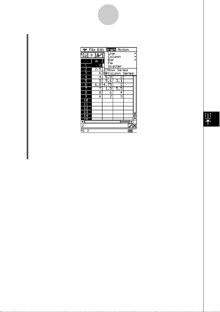
u [Graph] - [Column Series]
Selecting this option treats each column as a separate set of data. The value in each row is
plotted as a vertical axis value. The following shows a typical clustered column graph while
[Column Series] is selected, and the data that produced it.
Graph Window Menus and Toolbar
The following describes the special menus and toolbar that appears whenever the
Spreadsheet application Graph window is on the display.
k O Menu
•See “Using the O Menu” on page 1-5-4 of your ClassPad 300 User’s Guide.
k Edit Menu
•See “Edit Menu” on page 2-1 of this User’s Guide.
20040801
Page 62

8-9
Graphing
k View Menu
Many of the [View] menu commands can also be executed by tapping Spreadsheet
application Graph window toolbar buttons.
To do this:
Change the function of the stylus so it can be
used to select and move points on the displayed G Select
graph
Start a box zoom operation Q Zoom Box
Activate the pan function for dragging the Graph
window with the stylus
Enlarge the display image W Zoom In
Reduce the size of the display image E Zoom Out
Adjust the size of the display image so it fits the
display
Toggle display of axes and coordinate values on
and off
Toggle line graph and scatter graph plot markers
on and off
Toggle line graph and scatter connecting lines
on and off
Tap this Or select this
toolbar button: [View] menu item:
T Pan
R Zoom to Fit
q Toggle Axes
—Markers
—Lines
k Type Menu
• The [Type] menu is identical to the [Graph] menu described on page 8-1.
k Series Menu
All of the [Series] menu commands can also be executed by tapping a Graph window toolbar
button.
•All of the [Series] menu operations are available only when there is a clustered line graph
or a clustered column graph on the Graph window.
• In all of the following cases, you first need to tap a plot point or a column to specify which
data you want to use for the operation you are about to perform.
20040801
Page 63

8-10
Graphing
To do this:
Tap this Or select this
toolbar button: [Series] menu item:
Display a linear regression curve d Trend - Linear
Display a quadratic regression curve f
Display a cubic regression curve g
Display a quartic regression curve h
Display a quintic regression curve j
x
Display an exponential Ae
B
regression curve k Trend - Exponential
Trend - Polynomial Quadratic
Trend - Polynomial Cubic
Trend - Polynomial Quartic
Trend - Polynomial Quintic
Display a logarithmic Aln(x) + B regression curve l Trend - Logarithmic
Display a power AxB regression curve ; Trend - Power
Convert the data of the selected column to a
line graph
Convert the data of the selected line to a column
graph
z Line
' Column
Important!
•Exponential and logarithmic regression curves ignore negative values when calculating the
curve. A message appears in the status bar to let you know when negative values are
ignored.
20041001
Page 64

8-11
Graphing
Basic Graphing Steps
The following are the basic steps for graphing spreadsheet data.
u ClassPad Operation
(1) Input the data you want to graph into the spreadsheet.
(2) Use the [Graph] menu to specify whether you want to graph the data by row or by
column.
To do this: Select this [Graph] menu option:
Graph the data by row Row Series
Graph the data by column Column Series
•See “Graph Menu” on page 8-1 for more information.
(3) Select the cells that contain the data you want to graph.
•See “Selecting Cells” on page 3-5 for information about selecting data.
20040801
Page 65
8-12
Graphing
(4) On the [Graph] menu, select the type of graph you want to draw. Or you can tap the
applicable icon on the toolbar.
• This draws the selected graph. See “Graph Menu” on page 8-1 for examples of the
different types of graphs that are available.
•You can change to another type of graph at any time by selecting the graph type you
want on the [Type] menu. Or you can tap the applicable icon on the toolbar.
20040801
Page 66

8-13
Graphing
Other Graph Window Operations
This section provides more details about the types of operations you can perform while the
Graph window is on the display.
u To show or hide lines and markers
(1) While a line graph or a scatter graph is on the Graph window, tap the [View] menu.
Lines and markers both turned on
(2) Tap the [Markers] or [Lines] item to toggle it between show (checkbox selected) and
hide (checkbox cleared).
Lines turned on, markers hidden
Markers turned on, lines hidden
• Line and scatter graphs can have markers only, lines only, or both markers and lines.
You cannot turn off both markers and lines at the same time.
20040801
Page 67

8-14
Graphing
u To change a line in a clustered line graph to a column graph
(1) Draw the clustered line graph.
(2) With the stylus, tap any data point on the line you wish to change to a column graph.
(3) On the [Series] menu, tap [Column].
•You could also tap the down arrow button next to the third tool button from the left,
and then tap '.
•You can change more than one line to a column graph, if you want.
•You can change a column graph back to a line graph by selecting one of its columns
and tapping [Line] on the [Series] menu.
20040801
Page 68

8-15
Graphing
u To change a column in a clustered column graph to a line
(1) Draw the clustered column graph.
(2) With the stylus, tap any one of the columns you wish to change to a line graph.
(3) On the [Series] menu, tap [Line].
•You could also tap the down arrow button next to the third tool button from the left,
and then tap z.
•You can change more than one column to a line graph, if you want.
•You can change a line graph back to a column graph by selecting one of its data
points and tapping [Column] on the [Series] menu.
20040801
Page 69

8-16
Graphing
u To display a regression curve
(1) Draw a clustered line graph or clustered column graph.
•A regression curve can be drawn for a line, column, or scatter graph only.
• The above shows a stacked line graph.
(2) With the stylus, tap any point of the data for which you want to draw the regression
curve.
(3) Use the [Series] menu to select the type of regression curve you want.
•You could also tap the down arrow button next to the third tool button from the left,
and tap an icon to select the regression curve type.
•See “Series Menu” on page 8-9 for information about regression curve types.
•Here, we will select quartic regression.
20040801
Page 70

8-17
Graphing
• This causes the applicable regression curve to appear in the Graph window.
•Tapping the regression curve selects it and displays its equation in the status bar.
•You can drag and drop the regression curve to a cell or the edit box in the
Spreadsheet window.
•To delete all displayed regression curves, select [Clear All] on the [Edit] menu.
•Note that regression curves are also deleted automatically if you change to another
graph style.
20040801
Page 71

8-18
Graphing
u To find out the percentage of data for each pie graph section
(1) While the display is split between the pie graph and the Spreadsheet windows, tap the
pie graph to select it.
(2) On the [Edit] menu, tap [Copy].
(3) Tap the Spreadsheet window to make it active.
(4) Tap the cell where you want to paste the data.
• The cell you tap will be the upper left cell of the group of cells that will be pasted.
(5) On the [Edit] menu, tap [Paste].
• This pastes two columns of values. The numbers in the left column are pie graph
section numbers. The values in the right column are the percentages that the data in
each section of the pie graph represents.
u To change View Window settings
(1) While a graph is on the Graph window, tap O, [Settings], and then [View Window].
• This displays the current View Window settings.
(2) Change the View Window settings, if you want.
•See “Configuring View Window Parameters for the Graph Window” on page 3-2-1 of
the ClassPad 300 User’s Guide for information about using the View Window.
(3) After the settings are the way you want, tap [OK] to apply them.
20040801
Page 72
8-19
Graphing
u To change the appearance of the axes
While a graph is on the Graph window, select [Toggle Axes] on the [View] menu or tap the
q toolbar button to cycle through axes settings in the following sequence: axes on → axes
and values on → axes and values off →.
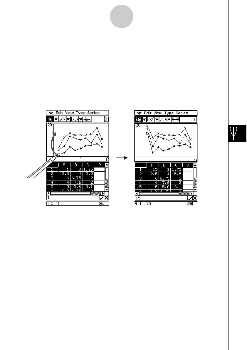
u To change the appearance of a graph by dragging a point
While a graph is on the Graph window, use the stylus to drag any one of its data points to
change the configuration of the graph.
•You can change curves, make bars or columns longer or shorter, or change the size of pie
graph sections.
•Changing a graph automatically changes the graph’s data on the Spreadsheet window.
20040801
ChangesDrag
Page 73

8-20
Graphing
• If a regression curve is displayed for the data whose graph is being changed by dragging,
the regression curve also changes automatically in accordance with the drag changes.
•When you edit data in the spreadsheet and press E, your graph will update automatically.
Important!
•You can drag a point only if it corresponds to a fixed value on the spreadsheet. You cannot
drag a point if it corresponds to a formula.
20040801
Page 74

CASIO COMPUTER CO., LTD.
6-2, Hon-machi 1-chome
Shibuya-ku, Tokyo 151-8543, Japan
SA0410-B
 Loading...