

Page 1

ClassPad II
fx-CP400
E
User’s Guide
CASIO Education website URL
http://edu.casio.com
Access the URL below and register as a user.
http://edu.casio.com/dl/
Page 2
Be sure to keep physical records of all important data!
Low battery power or incorrect replacement of the batteries that power the ClassPad can cause the data stored
in memory to be corrupted or even lost entirely. Stored data can also be affected by strong electrostatic charge
or strong impact. It is up to you to keep backup copies of data to protect against its loss.
Backing Up Data
ClassPad data can be converted to a VCP file or XCP file and transferred to a computer for storage. For details,
see “15-2 Performing Data Communication between the ClassPad and a Personal Computer”.
• Be sure to keep all user documentation handy for future reference.
• The sample screens shown in this manual are for illustrative purposes only, and may not be exactly the
same as the screens actually produced by the ClassPad.
• The contents of this manual are subject to change without notice.
• No part of this manual may be reproduced in any form without the express written consent of the
manufacturer.
• The options described in “Chapter 15: Performing Data Communication” in this manual may not be
available in certain geographic areas. For full details on availability in your area, contact your nearest
CASIO dealer or distributor.
• In no event shall CASIO Computer Co., Ltd. be liable to anyone for special, collateral, incidental, or
consequential damages in connection with or arising out of the purchase or use of these materials.
Moreover, CASIO Computer Co., Ltd. shall not be liable for any claim of any kind whatsoever against the
use of these materials by any other party.
• Windows® and Windows Vista® are registered trademarks or trademarks of Microsoft Corporation in the
United States and/or other countries.
• Mac, Macintosh, and Mac OS are registered trademarks or trademarks of Apple Inc. in the United States
and/or other countries.
• Fugue © 1999 – 2012 Kyoto Software Research, Inc. All rights reserved.
• Company and product names used in this manual may be registered trademarks or trademarks of their
respective owners.
• Note that trademark ™ and registered trademark ® are not used within the text of this manual.
2
Page 3
Contents
About This User’s Guide ............................................................................................................................9
Chapter 1: Basics ................................................................................................................ 10
1-1 General Guide .........................................................................................................................10
ClassPad at a Glance...............................................................................................................................10
Turning Power On or Off .......................................................................................................................... 11
1-2 Power Supply ..........................................................................................................................11
1-3 Built-in Application Basic Operations .................................................................................. 12
Using the Application Menu......................................................................................................................12
Built-in Applications ..................................................................................................................................12
Application Window ..................................................................................................................................13
Using the O Menu ...................................................................................................................................14
Interpreting Status Bar Information ..........................................................................................................15
Pausing and Terminating an Operation ....................................................................................................15
1-4 Input .........................................................................................................................................15
Using the Soft Keyboard ..........................................................................................................................15
Soft Keyboard Key Sets ........................................................................................................................... 16
Input Basics .............................................................................................................................................. 17
Various Soft Keyboard Operations ........................................................................................................... 20
1-5 ClassPad Data ......................................................................................................................... 25
Data Types and Storage Locations (Memory Areas) ............................................................................... 25
Main Memory Data Types ........................................................................................................................ 26
Main Memory Folders ...............................................................................................................................26
Using Variable Manager ........................................................................................................................... 27
Managing Application Files ......................................................................................................................30
1-6 Creating and Using Variables ................................................................................................ 31
Creating a New Variable ..........................................................................................................................31
Variable Usage Example .......................................................................................................................... 32
“library” Folder Variables .......................................................................................................................... 32
Rules Governing Variable Access ............................................................................................................ 33
1-7 Configuring Application Format Settings .............................................................................34
Application Format Settings .....................................................................................................................34
Initializing All Application Format Settings ................................................................................................40
1-8 When you keep having problems… ...................................................................................... 41
Chapter 2: Main Application ............................................................................................... 42
Main Application-Specific Menus and Buttons ......................................................................................... 42
2-1 Basic Calculations .................................................................................................................. 42
Arithmetic Calculations and Parentheses Calculations ............................................................................ 42
Using the e Key .................................................................................................................................. 43
Omitting the Multiplication Sign ................................................................................................................ 43
Using the Answer Variable (ans) .............................................................................................................. 43
Assigning a Value to a Variable ...............................................................................................................43
Calculation Priority Sequence .................................................................................................................. 44
Calculation Modes .................................................................................................................................... 44
2-2 Using the Calculation History ................................................................................................46
2-3 Function Calculations ............................................................................................................ 46
2-4 List Calculations ..................................................................................................................... 55
Inputting List Data in the Work Area .........................................................................................................55
LIST Variable Element Operations ........................................................................................................... 55
3
Page 4
Using a List in a Calculation ..................................................................................................................... 55
Using a List to Assign Different Values to Multiple Variables ................................................................... 55
2-5 Matrix and Vector Calculations ............................................................................................. 56
Inputting Matrix Data ................................................................................................................................ 56
Performing Matrix Calculations ................................................................................................................56
Using a Matrix to Assign Different Values to Multiple Variables ...............................................................57
2-6 Specifying a Number Base ....................................................................................................57
Binary, Octal, Decimal, and Hexadecimal Calculation Ranges ................................................................ 57
Selecting a Number Base.........................................................................................................................58
Arithmetic Operations ............................................................................................................................... 58
Bitwise Operations ...................................................................................................................................58
Using the baseConvert Function (Number System Transform) ...............................................................59
2-7 Using the Action Menu ........................................................................................................... 59
Abbreviations and Punctuation Used in This Section ...............................................................................59
Example Screenshots ..............................................................................................................................60
Using the Transformation Submenu .........................................................................................................60
Using the Advanced Submenu ................................................................................................................. 62
Using the Calculation Submenu ............................................................................................................... 65
Using the Complex Submenu ...................................................................................................................67
Using the List-Create Submenu ............................................................................................................... 69
Using the List-Statistics and List-Calculation Submenus ......................................................................... 70
Using the Matrix-Create Submenu ........................................................................................................... 73
Using the Matrix-Calculation and Matrix-Row&Column Submenus ......................................................... 74
Using the Vector Submenu ......................................................................................................................77
Using the Equation/Inequality Submenu ................................................................................................. 79
Using the Assistant Submenu .................................................................................................................. 82
Using the Distribution/Inv.Dist Submenu .................................................................................................. 82
Using the Financial Submenu ..................................................................................................................88
Using the Command Submenu ................................................................................................................ 88
2-8 Using the Interactive Menu ................................................................................................... 89
Interactive Menu Example ........................................................................................................................ 89
Using the “apply” Command .....................................................................................................................89
2-9 Using the Main Application in Combination with Other Applications ...............................89
Using Another Application’s Window ........................................................................................................90
Using the Stat Editor Window ...................................................................................................................90
Using the Geometry Window ....................................................................................................................91
2-10 Using Verify ........................................................................................................................... 92
2-11 Using Probability ..................................................................................................................92
2-12 Running a Program in the Main Application ...................................................................... 93
Chapter 3: Graph & Table Application ............................................................................... 95
Graph & Table Application-Specific Menus and Buttons ..........................................................................95
3-1 Storing Functions ................................................................................................................... 97
Using Graph Editor Sheets.......................................................................................................................97
Storing a Function .................................................................................................................................... 97
Graphing a Stored Function ..................................................................................................................... 98
Shading the Region Bounded by Two Expressions ................................................................................. 99
Overlaying Two Inequalities in an Intersection Plot / Union Plot .............................................................. 99
Saving Graph Editor Data to Graph Memory .........................................................................................100
3-2 Using the Graph Window ..................................................................................................... 100
Configuring View Window Parameters for the Graph Window ............................................................... 100
Using View Window Memory ..................................................................................................................102
Panning the Graph Window ...................................................................................................................103
4
Page 5
Scrolling the Graph Window ................................................................................................................... 103
Zooming the Graph Window ...................................................................................................................103
Using Quick Zoom .................................................................................................................................. 104
Using Built-in Functions for Graphing .....................................................................................................104
Saving a Screenshot of a Graph ............................................................................................................ 105
Adjusting the Lightness (Fade I/O) of the Graph Window Background Image ....................................... 105
3-3 Using Table & Graph.............................................................................................................106
Generating a Number Table ................................................................................................................... 106
Showing Linked Displays of Number Table Coordinates and Graph Coordinates (Link Trace) ............. 107
Generating Number Table Values from a Graph ....................................................................................108
Generating a Summary Table ................................................................................................................ 108
3-4 Using Trace ...........................................................................................................................109
Using Trace to Read Graph Coordinates ............................................................................................... 109
3-5 Using the Sketch Menu ........................................................................................................ 110
Using Sketch Menu Commands ............................................................................................................. 110
3-6 Analyzing a Function Used to Draw a Graph .....................................................................112
What You Can Do Using the G-Solve Menu Commands ....................................................................... 112
Using G-Solve Menu Commands ........................................................................................................... 112
3-7 Modifying a Graph ................................................................................................................ 113
Chapter 4: Conics Application ..........................................................................................114
Conics Application-Specific Menus and Buttons .................................................................................... 114
4-1 Inputting an Equation ........................................................................................................... 115
4-2 Drawing a Conics Graph ...................................................................................................... 115
Drawing a Parabola ................................................................................................................................ 115
Drawing a Circle ..................................................................................................................................... 116
Drawing an Ellipse..................................................................................................................................116
Drawing a Hyperbola .............................................................................................................................. 116
Drawing a General Conics .....................................................................................................................116
4-3 Using G-Solve to Analyze a Conics Graph ......................................................................... 116
What You Can Do Using the G-Solve Menu Commands ....................................................................... 116
Using G-Solve Menu Commands ........................................................................................................... 117
Chapter 5: Differential Equation Graph Application........................................................118
Differential Equation Editor Window-Specific Menus and Buttons ......................................................... 118
Differential Equation Graph Window-Specific Menus and Buttons ........................................................118
5-1 Graphing a Differential Equation ......................................................................................... 119
Graphing a First Order Differential Equation .......................................................................................... 119
Graphing a Second Order Differential Equation ..................................................................................... 120
Graphing an Nth-order Differential Equation .......................................................................................... 120
Configuring and Modifying Initial Conditions .......................................................................................... 121
Configuring Differential Equation Graph View Window Parameters ......................................................122
5-2 Drawing f ( x) Type Function Graphs and Parametric Function Graphs ...........................123
5-3 Using Trace to Read Graph Coordinates ............................................................................123
5-4 Graphing an Expression or Value by Dropping It into the Differential Equation
Graph Window ......................................................................................................................124
Chapter 6: Sequence Application .................................................................................... 125
Sequence Application-Specific Menus and Buttons ............................................................................... 125
6-1 Recursive and Explicit Form of a Sequence ...................................................................... 126
Generating a Number Table ................................................................................................................... 126
Determining the General Term of a Recursion Expression .................................................................... 127
5
Page 6
Calculating the Sum of a Sequence ....................................................................................................... 127
6-2 Graphing a Recursion ..........................................................................................................127
Chapter 7: Statistics Application ..................................................................................... 128
7-1 Using Stat Editor ...................................................................................................................128
Basic List Operations .............................................................................................................................128
Menus and Buttons Used for List Editing ............................................................................................... 129
7-2 Drawing a Statistical Graph ................................................................................................. 130
Operation Flow Up to Statistical Graphing ............................................................................................. 130
Graphing Single-Variable Statistical Data .............................................................................................. 131
Graphing Paired-Variable Statistical Data .............................................................................................. 132
Overlaying a Regression Graph on a Scatter Plot .................................................................................134
Overlaying a Function Graph on a Statistical Graph .............................................................................. 135
Stat Graph Window Menus and Buttons ................................................................................................ 135
7-3 Performing Basic Statistical Calculations ..........................................................................136
Calculating Statistical Values ................................................................................................................. 136
Performing Regression Calculations ...................................................................................................... 138
Viewing the Results of the Last Statistical Calculation Performed (DispStat) ........................................ 139
7-4 Performing Advanced Statistical Calculations .................................................................. 139
Performing Test, Confidence Interval and Distribution Calculations Using the Wizard .......................... 139
Tests.......................................................................................................................................................141
Confidence Intervals...............................................................................................................................143
Distributions............................................................................................................................................145
Input and Output Terms .........................................................................................................................148
Chapter 8: Geometry Application .................................................................................... 150
Geometry Application-Specific Menus and Buttons ............................................................................... 150
Configuring Geometry View Window Settings ........................................................................................151
About the Geometry Format Dialog Box ................................................................................................151
8-1 Drawing Figures ....................................................................................................................151
Drawing a Figure .................................................................................................................................... 151
Inserting Text Strings into the Screen .................................................................................................... 155
Attaching an Angle Measurement to a Figure ........................................................................................ 155
Displaying the Measurements of a Figure .............................................................................................. 155
Displaying the Result of a Calculation that Uses On-screen Measurement Values ............................... 156
Using the Special Polygon Submenu ..................................................................................................... 156
Using the Construct Submenu ...............................................................................................................157
8-2 Editing Figures ......................................................................................................................161
Selecting and Deselecting Figures ......................................................................................................... 161
Moving and Copying Figures ..................................................................................................................162
Pinning an Annotation on the Geometry Window ...................................................................................162
Specifying the Number Format of a Measurement .................................................................................162
Specifying the Color and Line Type of a Displayed Object .................................................................... 163
Changing the Display Priority of Objects ................................................................................................ 163
8-3 Using the Measurement Box ...............................................................................................164
Viewing the Measurements of a Figure .................................................................................................. 164
Specifying and Constraining a Measurement of a Figure ......................................................................165
Changing a Label or Adding a Name to an Element .............................................................................. 166
8-4 Working with Animations .....................................................................................................167
Using Animation Commands .................................................................................................................. 167
8-5 Using the Geometry Application with Other Applications ................................................170
Drag and Drop ........................................................................................................................................ 170
Copy and Paste ...................................................................................................................................... 170
6
Page 7
Chapter 9: Numeric Solver Application ........................................................................... 171
Numeric Solver Application-Specific Menus and Buttons ......................................................................171
Inputting an Equation .............................................................................................................................171
Solving an Equation ...............................................................................................................................171
Chapter 10: eActivity Application .................................................................................... 173
eActivity Application-Specific Menus and Buttons ..................................................................................173
10-1 Creating an eActivity .......................................................................................................... 173
Basic Steps for Creating an eActivity ..................................................................................................... 173
Inserting Data into an eActivity ............................................................................................................... 174
Inserting an Application Data Strip ......................................................................................................... 175
Inserting a Geometry Link Row .............................................................................................................. 177
10-2 Transferring eActivity Files ................................................................................................178
File Compatibility .................................................................................................................................... 178
Transferring eActivity Files between a ClassPad Unit and a Computer ................................................. 178
Transferring eActivity Files between Two ClassPad Units ..................................................................... 178
Chapter 11: Financial Application .................................................................................... 179
11-1 Financial Application Basic Operations ...........................................................................179
Page Operations ....................................................................................................................................180
Configuring Financial Application Settings ............................................................................................. 181
11-2 Performing Financial Calculations ....................................................................................182
11-3 Calculation Formulas .........................................................................................................182
Simple Interest .......................................................................................................................................182
Compound Interest ................................................................................................................................. 183
Cash Flow ..............................................................................................................................................183
Amortization ...........................................................................................................................................184
Interest Conversion ................................................................................................................................ 184
Cost/Sell/Margin .....................................................................................................................................185
Depreciation ...........................................................................................................................................185
Bond Calculation .................................................................................................................................... 185
Break-Even Point ...................................................................................................................................186
Margin of Safety ..................................................................................................................................... 186
Financial Leverage ................................................................................................................................. 186
Operating Leverage................................................................................................................................186
Combined Leverage ............................................................................................................................... 186
Quantity Conversion ............................................................................................................................... 186
11-4 Financial Calculation Functions ........................................................................................187
11-5 Input and Output Field Names ...........................................................................................188
Chapter 12: Program Application .................................................................................... 189
Program Application-Specific Menus and Buttons ................................................................................. 189
12-1 Creating and Running Program ........................................................................................190
Creating a Program ................................................................................................................................ 190
Running a Program ................................................................................................................................ 192
Terminating Program Execution ............................................................................................................. 193
Creating a Text File ................................................................................................................................ 193
Using Text Files......................................................................................................................................194
Converting a Text File to a Program File ................................................................................................194
Converting a Program File to an Executable File ................................................................................... 194
12-2 Debugging a Program ........................................................................................................ 195
Debugging After an Error Message Appears .........................................................................................195
Debugging a Program Following Unexpected Results ........................................................................... 195
7
Page 8
Editing a Program...................................................................................................................................195
12-3 User-defined Functions ......................................................................................................196
Creating a New User-defined Function .................................................................................................. 196
Executing a User-defined Function ........................................................................................................ 197
Editing a User-defined Function ............................................................................................................. 197
12-4 Program Command Reference .......................................................................................... 198
Using This Reference ............................................................................................................................. 198
Syntax Conventions ...............................................................................................................................198
Command List ........................................................................................................................................ 199
12-5 Including ClassPad Functions in Programs ....................................................................218
Including Graphing Functions in a Program ........................................................................................... 218
Including Table & Graph Functions in a Program ..................................................................................218
Including Recursion Table and Recursion Graph Functions in a Program ............................................218
Including Statistical Graphing and Calculation Functions in a Program ................................................. 218
Including Financial Calculation Functions in a Program .........................................................................218
Chapter 13: Spreadsheet Application .............................................................................. 219
Spreadsheet Window-Specific Menus and Buttons ...............................................................................219
Changing the Width of a Column ...........................................................................................................220
Option Settings ....................................................................................................................................... 221
13-1 Inputting and Editing Cell Contents ..................................................................................221
Selecting Cells........................................................................................................................................221
Inputting Data into a Cell ........................................................................................................................ 222
Inputting a Formula ................................................................................................................................222
Inputting a Cell Reference ...................................................................................................................... 223
Cell Data Types (Text Data and Calculation Data) ................................................................................224
Inputting a Constant into a Calculation Data Type Cell .......................................................................... 224
Using the Cell Viewer Window ............................................................................................................... 226
Changing the Text Color and Fill Color of Specific Cells ........................................................................226
Copying or Cutting Cells and Pasting Them to Another Location .......................................................... 227
Recalculating Spreadsheet Expressions ................................................................................................ 227
Importing and Exporting Variable Values ............................................................................................... 228
13-2 Graphing ..............................................................................................................................229
Basic Graphing Steps ............................................................................................................................229
Column Series and Row Series .............................................................................................................229
Graph Colors and Color Link .................................................................................................................. 230
Spreadsheet Graph Window-Specific Menus and Buttons ....................................................................231
Graph Menu and Graph Examples .........................................................................................................232
Regression Graph Operations (Curve Fitting) ........................................................................................ 234
Other Graph Window Operations ........................................................................................................... 236
13-3 Statistical Calculations ......................................................................................................237
Single-variable, Paired-variable and Regression Calculations ...............................................................237
Test and Interval Calculations ................................................................................................................ 238
Distribution Calculations ......................................................................................................................... 240
About DispStat Command ...................................................................................................................... 241
13-4 Cell and List Calculations .................................................................................................. 241
Using the Cell Calculation Functions ......................................................................................................241
Using the List Calculation Functions ...................................................................................................... 242
Chapter 14: System Application ...................................................................................... 243
14-1 Managing Memory Usage ..................................................................................................243
Using the Storage Sheet ........................................................................................................................ 243
Using the Main Memory Sheet and eActivity Sheet ............................................................................... 244
8
Page 9
14-2 Configuring System Settings ............................................................................................245
System Application Menus and Buttons ................................................................................................. 245
Configuring System Settings .................................................................................................................. 245
Chapter 15: Performing Data Communication ................................................................ 249
15-1 Data Communication Overview ......................................................................................... 249
Using the ClassPad Communication Application ................................................................................... 249
Select Connection Mode Dialog Box ...................................................................................................... 250
15-2 Performing Data Communication between the ClassPad and a Personal Computer ..250
Connecting and Disconnecting with a Computer in the USB Flash Mode .............................................251
Transferring Data between the ClassPad and a Personal Computer ....................................................252
Auto Import of VCP Files ........................................................................................................................ 253
Rules for ClassPad Files and Folders .................................................................................................... 253
VCP and XCP File Operations ............................................................................................................... 253
15-3 Performing Data Communication between Two ClassPads ........................................... 255
Connecting to Another ClassPad Unit .................................................................................................... 255
Transferring Data between Two ClassPads ........................................................................................... 255
Communication Standby ........................................................................................................................ 257
Interrupting an Ongoing Data Communication Operation ...................................................................... 257
15-4 Connecting the ClassPad to an EA-200 Data Analyzer ...................................................257
Connecting a ClassPad to a CASIO EA-200 Data Analyzer .................................................................. 257
15-5 Connecting the ClassPad to a Projector .......................................................................... 258
Projecting ClassPad Screen Contents from a Projector .........................................................................258
Precautions when Connecting................................................................................................................258
Appendix ............................................................................................................................ 259
Character Code Table .................................................................................................................. 259
System Variable Table ................................................................................................................. 263
Graph Types and Executable Functions.................................................................................... 266
Error and Warning Message Tables ........................................................................................... 267
Error Message Table ............................................................................................................................. 267
Warning Message Table ........................................................................................................................269
Low Memory Error Processing ............................................................................................................... 270
Resetting and Initializing the ClassPad ..................................................................................... 270
Number of Digits and Precision ................................................................................................. 271
Number of Digits.....................................................................................................................................271
Precision.................................................................................................................................................271
Display Brightness and Battery Life .......................................................................................... 272
Display Brightness..................................................................................................................................272
Battery Life ............................................................................................................................................. 272
Specifications ..............................................................................................................................272
About This User’s Guide
• The four digit boldface example numbers (such as 0201 ) that appear in Chapters 2 through 13 indicate
operation examples that can be found in the separate “Examples” booklet. You can use the “Examples”
booklet in conjunction with this manual by referring to the applicable example numbers.
• In this manual, cursor key operations are indicated as f, c, d, e (1-1 General Guide).
9
Page 10
Chapter 1: Basics
This chapter provides a general overview of the ClassPad and application operations, as well as information
about input operations, the handling of data (variables and folders), file operations, and how to configure
application format settings.
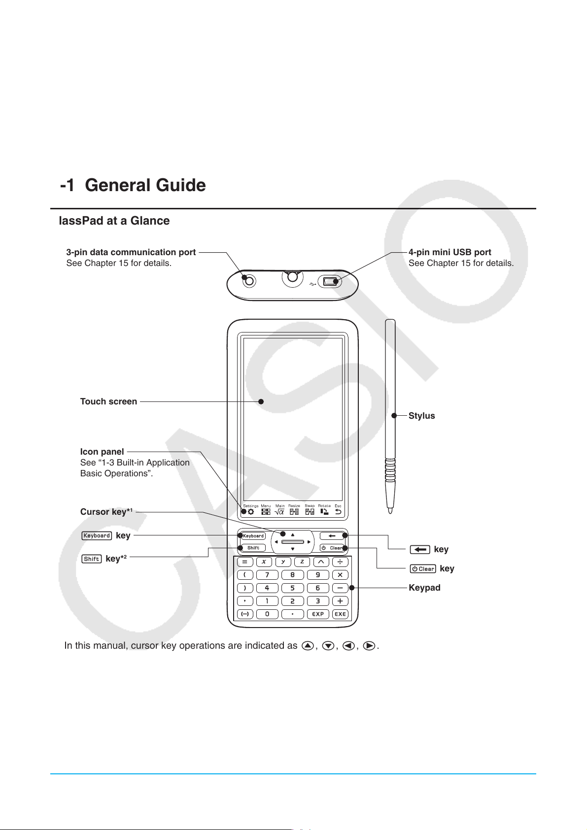
1-1 General Guide
ClassPad at a Glance
3-pin data communication port
See Chapter 15 for details.
Touch screen
Icon panel
See “1-3 Built-in Application
Basic Operations”.
Cursor key*
k key
f key*
1
2
4-pin mini USB port
See Chapter 15 for details.
Stylus
K key
c key
Keypad
*1 In this manual, cursor key operations are indicated as f, c, d, e.
*2 Certain functions (cut, paste, undo, etc.) or key input operations can be assigned to key combinations that
consist of pressing the f key and a keypad key. For more information, see “14-2 Configuring System
Settings”.
Chapter 1: Basics 10
Page 11
Turning Power On or Off
While the ClassPad is turned off, press c to turn it on.
To turn off the ClassPad, press f and then c.
Auto Power Off
The ClassPad also has an Auto Power Off feature. This feature automatically turns the ClassPad off when it is
idle for a specified amount of time. For details, see “To configure power properties” on page 246.
Note
Any temporary information in ClassPad RAM (graphs drawn on an application’s graph window, a dialog box
displayed, etc.) is retained for approximately 30 seconds whenever power is turned off manually or by Auto
Power Off. This means you will be able to restore the temporary information in RAM if you turn ClassPad back
on within about 30 seconds after it is turned off. After about 30 seconds, the temporary information in RAM is
cleared automatically, so turning ClassPad back on will display the startup screen of the application you were
using when you last turned it off, and the previous information in RAM will no longer be available.
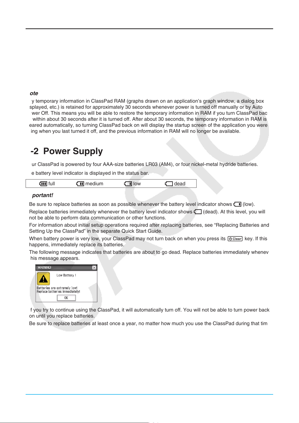
1-2 Power Supply
Your ClassPad is powered by four AAA-size batteries LR03 (AM4), or four nickel-metal hydride batteries.
The battery level indicator is displayed in the status bar.
full medium low dead
Important!
• Be sure to replace batteries as soon as possible whenever the battery level indicator shows (low).
• Replace batteries immediately whenever the battery level indicator shows
not be able to perform data communication or other functions.
• For information about initial setup operations required after replacing batteries, see “Replacing Batteries and
Setting Up the ClassPad” in the separate Quick Start Guide.
• When battery power is very low, your ClassPad may not turn back on when you press its c key. If this
happens, immediately replace its batteries.
• The following message indicates that batteries are about to go dead. Replace batteries immediately whenever
this message appears.
If you try to continue using the ClassPad, it will automatically turn off. You will not be able to turn power back
on until you replace batteries.
• Be sure to replace batteries at least once a year, no matter how much you use the ClassPad during that time.
(dead). At this level, you will
Note: The batteries that come with the ClassPad discharge slightly during shipment and storage. Because of
this, they may require replacement sooner than the normal expected battery life.
Backing Up Data
ClassPad data can be converted to a VCP file or XCP file and transferred to a computer for storage. For details,
see “15-2 Performing Data Communication between the ClassPad and a Personal Computer”.
Chapter 1: Basics 11
Page 12
1-3 Built-in Application Basic Operations
This section explains basic information and operations that are common to all of the built-in applications.
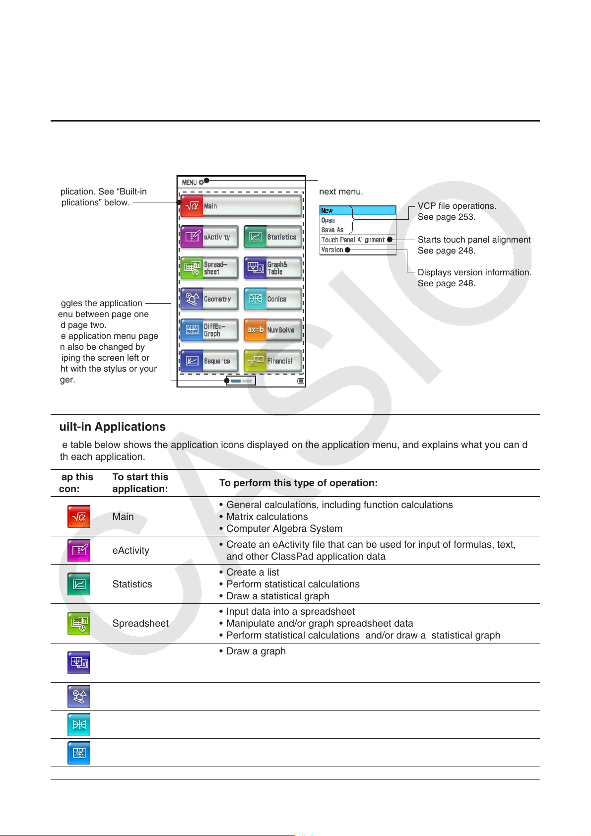
Using the Application Menu
Tapping m on the icon panel displays the application menu. You can perform the operations below with the
application menu.
Tap a button to start up an
application. See “Built-in
Applications” below.
Toggles the application
menu between page one
and page two.
The application menu page
can also be changed by
swiping the screen left or
right with the stylus or your
finger.
Tap here (or tap s on the icon panel) to display the
next menu.
VCP file operations.
See page 253.
Starts touch panel alignment.
See page 248.
Displays version information.
See page 248.
Built-in Applications
The table below shows the application icons displayed on the application menu, and explains what you can do
with each application.
Tap this
icon:
To start this
application:
To perform this type of operation:
• General calculations, including function calculations
Main
• Matrix calculations
• Computer Algebra System
eActivity
• Create an eActivity file that can be used for input of formulas, text,
and other ClassPad application data
• Create a list
Statistics
• Perform statistical calculations
• Draw a statistical graph
• Input data into a spreadsheet
Spreadsheet
• Manipulate and/or graph spreadsheet data
• Perform statistical calculations and/or draw a statistical graph
• Draw a graph
Graph & Table
• Register a function and create a table of solutions by substituting
different values for the function’s variables
Geometry
• Draw geometric figures
• Build animated figures
Conics • Draw the graph of a conics section
Differential Equation
Graph
• Draw vector fields and solution curves to explore differential equations
Chapter 1: Basics 12
Page 13
Tap this
icon:
To start this
application:
Numeric Solver
Sequence
Financial
Program
E-Con EA-200
To perform this type of operation:
• Obtain the value of any variable in an equation, without transforming
or simplifying the equation
• Perform sequence calculations
• Solve recursion expressions
• Perform simple interest, compound interest, and other financial
calculations
• Input a program or run a program
• Create a user-defined function
• Control the optionally available EA-200 Data Analyzer
(See the separate E-CON EA-200 User’s Guide.)
Communication • Exchange data with another ClassPad, a computer, or another device
• Manage ClassPad memory (main memory, eActivity area, storage
System
area)
• Configure system settings
Tip: You can also start up the Main application by tapping M on the icon panel.
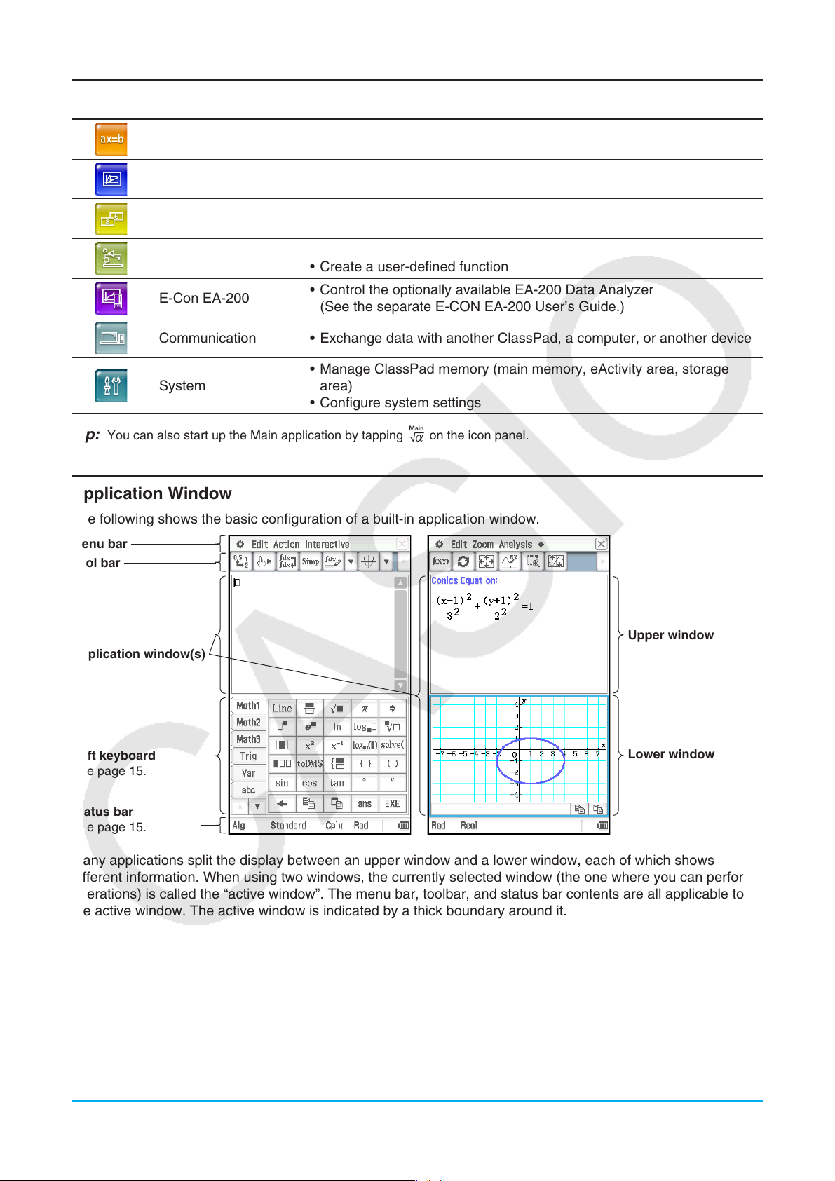
Application Window
The following shows the basic configuration of a built-in application window.
Menu bar
Tool bar
Upper window
Application window(s)
Soft keyboard
See page 15.
Status bar
See page 15.
Lower window
Many applications split the display between an upper window and a lower window, each of which shows
different information. When using two windows, the currently selected window (the one where you can perform
operations) is called the “active window”. The menu bar, toolbar, and status bar contents are all applicable to
the active window. The active window is indicated by a thick boundary around it.
You can perform the operations below on an Application window.
Chapter 1: Basics 13
Page 14
To do this: Perform this operation:
Switch the active window While a dual window is on the display, tap anywhere inside the window that does
not have a thick boundary around it to make it the active window. Note that you
cannot switch the active window while an operation is being performed in the
current active window.
Resize the active window
so it fills the display
Swap the upper and
lower windows
Close the active windows
While a dual window is on the display, tap r. This causes the active window to
fill the display. To return to the dual window display, tap r again.
While a dual window is on the display, tap S. This causes the upper window
to become the lower window, and vice versa. Swapping windows does not have
any effect on their active status. If the upper window is active when you tap S
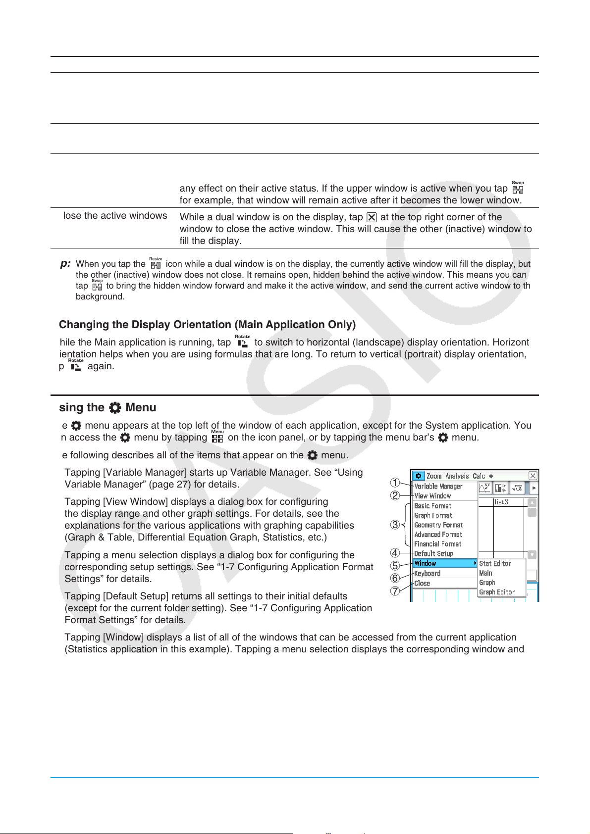
for example, that window will remain active after it becomes the lower window.
While a dual window is on the display, tap C at the top right corner of the
window to close the active window. This will cause the other (inactive) window to
fill the display.
Tip: When you tap the r icon while a dual window is on the display, the currently active window will fill the display, but
the other (inactive) window does not close. It remains open, hidden behind the active window. This means you can
tap S to bring the hidden window forward and make it the active window, and send the current active window to the
background.
u Changing the Display Orientation (Main Application Only)
While the Main application is running, tap g to switch to horizontal (landscape) display orientation. Horizontal
orientation helps when you are using formulas that are long. To return to vertical (portrait) display orientation,
tap g again.
Using the O Menu
The O menu appears at the top left of the window of each application, except for the System application. You
can access the O menu by tapping m on the icon panel, or by tapping the menu bar’s O menu.
The following describes all of the items that appear on the O menu.
1 Tapping [Variable Manager] starts up Variable Manager. See “Using
Variable Manager” (page 27) for details.
2 Tapping [View Window] displays a dialog box for configuring
the display range and other graph settings. For details, see the
explanations for the various applications with graphing capabilities
(Graph & Table, Differential Equation Graph, Statistics, etc.)
3 Tapping a menu selection displays a dialog box for configuring the
corresponding setup settings. See “1-7 Configuring Application Format
Settings” for details.
4 Tapping [Default Setup] returns all settings to their initial defaults
(except for the current folder setting). See “1-7 Configuring Application
Format Settings” for details.
5 Tapping [Window] displays a list of all of the windows that can be accessed from the current application
(Statistics application in this example). Tapping a menu selection displays the corresponding window and
makes it active.
6 Tap [Keyboard] to toggle display of the soft keyboard on or off.
7 Tapping [Close] closes the currently active window, except in the following cases.
• When only one window is on the display
• When the currently active window cannot be closed by the application being used
You cannot, for example, close the Graph Editor window from the Graph & Table application.
1
2
3
4
5
6
7
Chapter 1: Basics 14
Page 15
Interpreting Status Bar Information
The status bar appears along the bottom of the window of each application.
123
1 Information about the currently running application
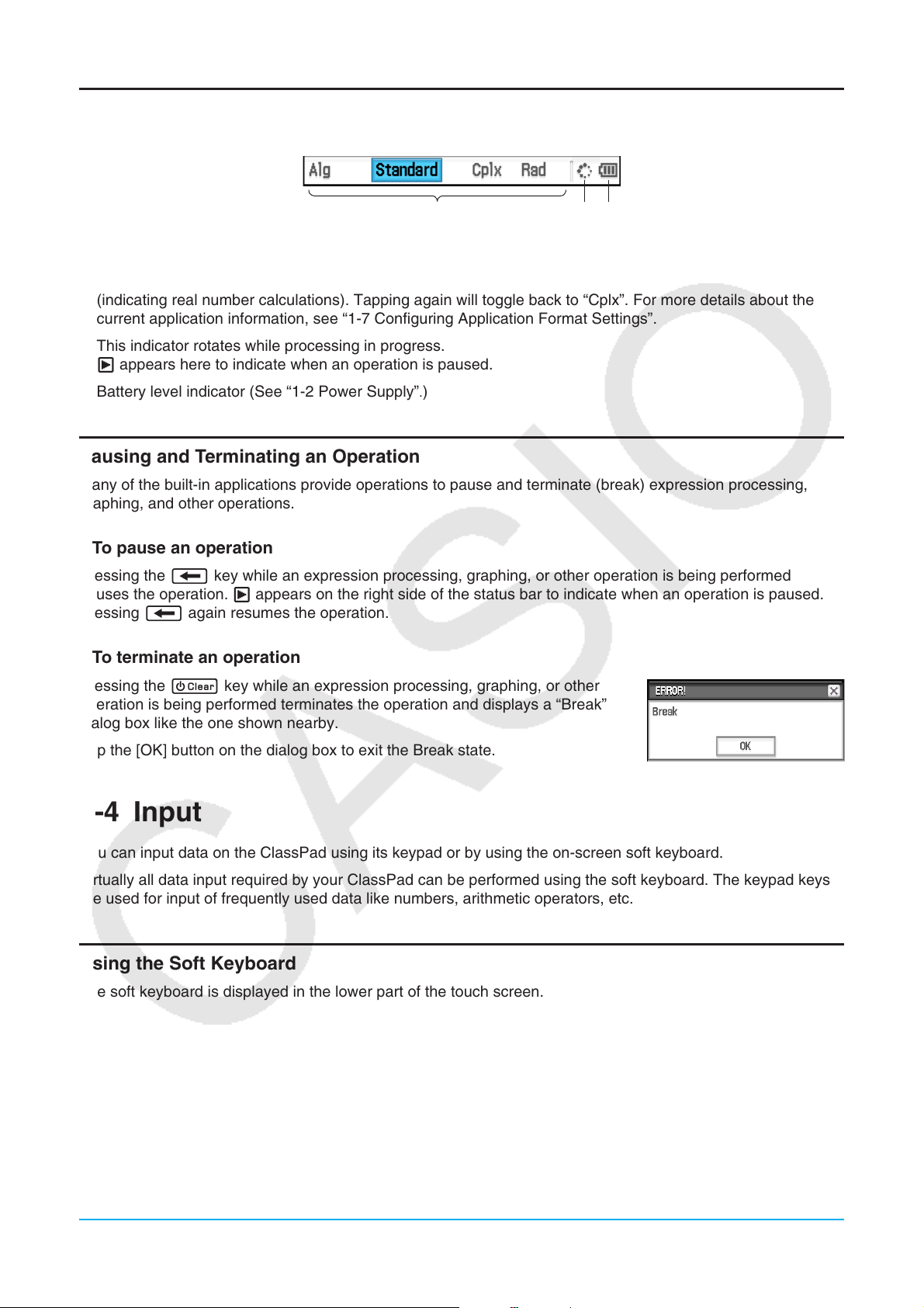
You can change the configuration of a setting indicated in the status bar by tapping it. Tapping “Cplx”
(indicating complex number calculations) while the Main application is running will toggle the setting to “Real”
(indicating real number calculations). Tapping again will toggle back to “Cplx”. For more details about the
current application information, see “1-7 Configuring Application Format Settings”.
2 This indicator rotates while processing in progress.
X appears here to indicate when an operation is paused.
3 Battery level indicator (See “1-2 Power Supply”.)
Pausing and Terminating an Operation
Many of the built-in applications provide operations to pause and terminate (break) expression processing,
graphing, and other operations.
u To pause an operation
Pressing the K key while an expression processing, graphing, or other operation is being performed
pauses the operation. X appears on the right side of the status bar to indicate when an operation is paused.
Pressing K again resumes the operation.
u To terminate an operation
Pressing the c key while an expression processing, graphing, or other
operation is being performed terminates the operation and displays a “Break”
dialog box like the one shown nearby.
Tap the [OK] button on the dialog box to exit the Break state.
1-4 Input
You can input data on the ClassPad using its keypad or by using the on-screen soft keyboard.
Virtually all data input required by your ClassPad can be performed using the soft keyboard. The keypad keys
are used for input of frequently used data like numbers, arithmetic operators, etc.
Using the Soft Keyboard
The soft keyboard is displayed in the lower part of the touch screen.
Chapter 1: Basics 15
Page 16
u To display the soft keyboard
When the soft keyboard is not on the touch screen, press the
k key, or tap the O menu and then tap [Keyboard]. This
causes the soft keyboard to appear.
• The soft keyboard has a number of different key sets such
as [Math1], [abc], and [Catalog], which you can use to input
of functions and text. To select a key set, tap one of the tabs
along the left side of the soft keyboard.
• Pressing the k key or tapping the O menu, and then
[Keyboard] again hides the soft keyboard.
Soft keyboard
Soft Keyboard Key Sets
The soft keyboard has a variety of different key sets that support various data input needs. Each of the
available key sets is shown below.
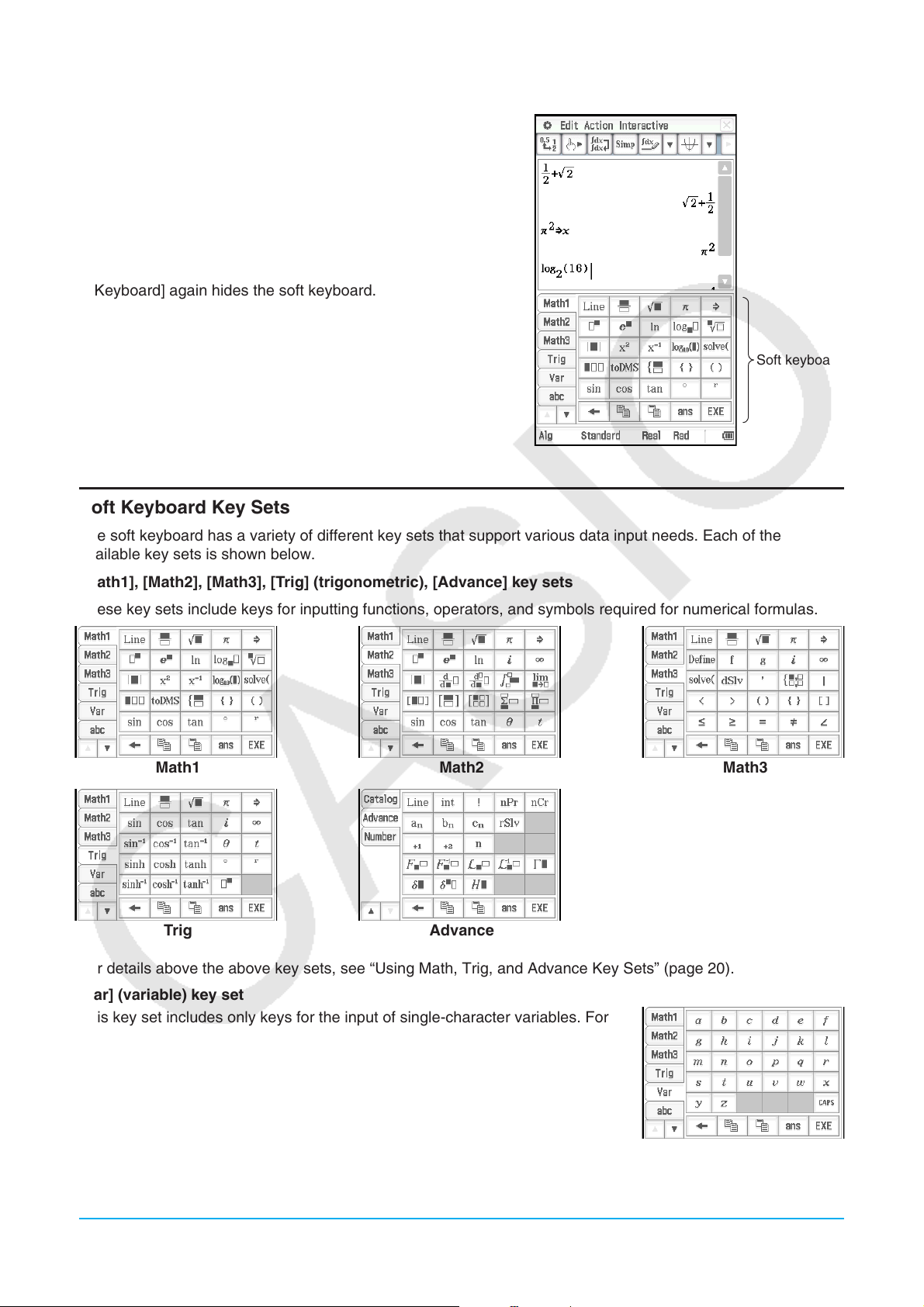
[Math1], [Math2], [Math3], [Trig] (trigonometric), [Advance] key sets
These key sets include keys for inputting functions, operators, and symbols required for numerical formulas.
Math1 Math2 Math3
Trig Advance
For details above the above key sets, see “Using Math, Trig, and Advance Key Sets” (page 20).
[Var] (variable) key set
This key set includes only keys for the input of single-character variables. For
more information, see “Using Single-character Variables” (page 23).
Chapter 1: Basics 16
Page 17
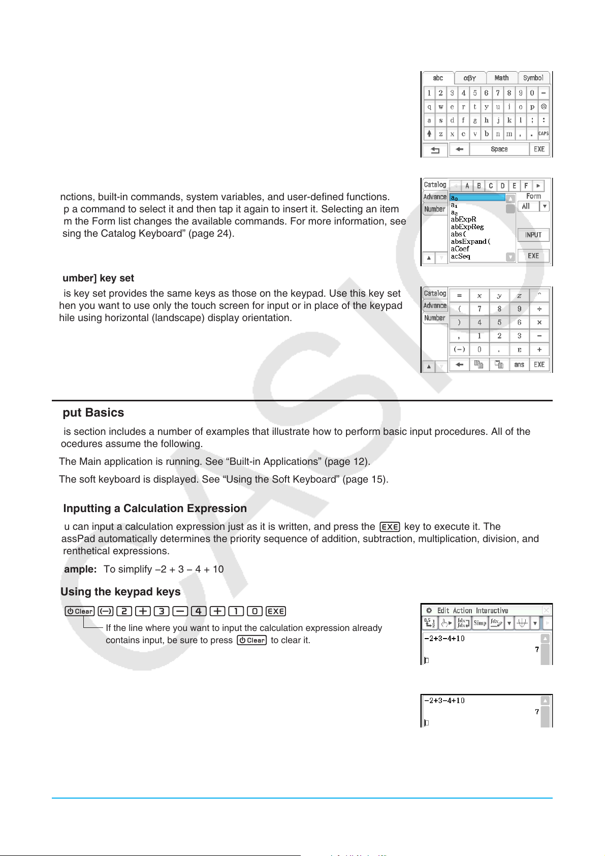
[abc] key set
Use this key set to input alphabetic characters. Tap one of the tabs along the
top of the keyboard (along the right when using horizontal display orientation)
to see additional characters, for example, tap [Math]. For more information, see
“Using the Alphabet Keyboard” (page 24).
[Catalog] key set
This key set provides a scrollable list that can be used to input built-in
functions, built-in commands, system variables, and user-defined functions.
Tap a command to select it and then tap it again to insert it. Selecting an item
from the Form list changes the available commands. For more information, see
“Using the Catalog Keyboard” (page 24).
[Number] key set
This key set provides the same keys as those on the keypad. Use this key set
when you want to use only the touch screen for input or in place of the keypad
while using horizontal (landscape) display orientation.
Input Basics
This section includes a number of examples that illustrate how to perform basic input procedures. All of the
procedures assume the following.
• The Main application is running. See “Built-in Applications” (page 12).
• The soft keyboard is displayed. See “Using the Soft Keyboard” (page 15).
kInputting a Calculation Expression
You can input a calculation expression just as it is written, and press the E key to execute it. The
ClassPad automatically determines the priority sequence of addition, subtraction, multiplication, division, and
parenthetical expressions.
Example: To simplify −2 + 3 − 4 + 10
u Using the keypad keys
cz2+3-4+10E
If the line where you want to input the calculation expression already
contains input, be sure to press
u Using the soft keyboard
Tap the keys of the [Number] keyboard to input the calculation expression.
c to clear it.
c4-c+d-e+baw
Chapter 1: Basics 17
Page 18
As shown in the above Example, you can input simple arithmetic calculations using either the keypad keys
or the soft keyboard. Input using the soft keyboard is required to input higher level calculation expressions,
functions, variables, etc. See Chapter 2 for more information about inputting expressions.
Tip: In some cases, the input expression and output expression (result) may not fit in
the display area. If this happens, tap the left or right arrows that appear on the
display to scroll the expression screen and view the part that does not fit.
You can also change the display orientation to horizontal
(landscape) for easier-to-read display of long input formulas
and calculation results. See “Changing the Display
Orientation (Main Application Only)” (page 14).
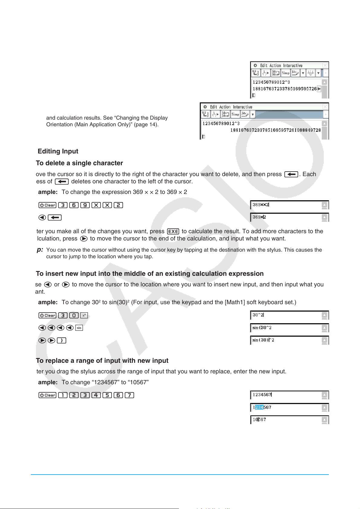
kEditing Input
u To delete a single character
Move the cursor so it is directly to the right of the character you want to delete, and then press K. Each
press of K deletes one character to the left of the cursor.
Example: To change the expression 369 × × 2 to 369 × 2
1. c369**2
2. dK
After you make all of the changes you want, press E to calculate the result. To add more characters to the
calculation, press e to move the cursor to the end of the calculation, and input what you want.
Tip: You can move the cursor without using the cursor key by tapping at the destination with the stylus. This causes the
cursor to jump to the location where you tap.
u To insert new input into the middle of an existing calculation expression
Use d or e to move the cursor to the location where you want to insert new input, and then input what you
want.
2
Example: To change 30
to sin(30)2 (For input, use the keypad and the [Math1] soft keyboard set.)
1. c30x
2. dddds
3. ee)
u To replace a range of input with new input
After you drag the stylus across the range of input that you want to replace, enter the new input.
Example: To change “1234567” to “10567”
1. c1234567
2. Drag the stylus across “234” to select it.
3. 0
Chapter 1: Basics 18
Page 19
k Using the Clipboard for Copy and Paste
You can copy (or cut) a function, command, or other input to the ClassPad’s clipboard, and then paste the
clipboard contents at another location. Performing a copy or cut operation causes the current clipboard
contents to be replaced by the newly copied or cut characters.
u To copy characters
1. Drag the stylus across the characters you want to copy to select them.
2. On the soft keyboard, tap p. Or tap the [Edit] menu and then tap [Copy].
• This puts a copy of the selected characters onto the clipboard.
u To cut characters
1. Drag the stylus across the characters you want to cut to select them.
2. Tap the [Edit] menu and then tap [Cut].
• This causes the selected characters to be deleted, and moves them onto the clipboard.
u To paste the clipboard contents
1. Move the cursor to the location where you want to paste the clipboard contents.
2. On the soft keyboard, tap q. Or tap the [Edit] menu and then tap [Paste].
• This pastes the clipboard contents at the current cursor location.
Tip: The clipboard contents remain on the clipboard after you paste them. This means you can paste the current contents
as many times as you like.
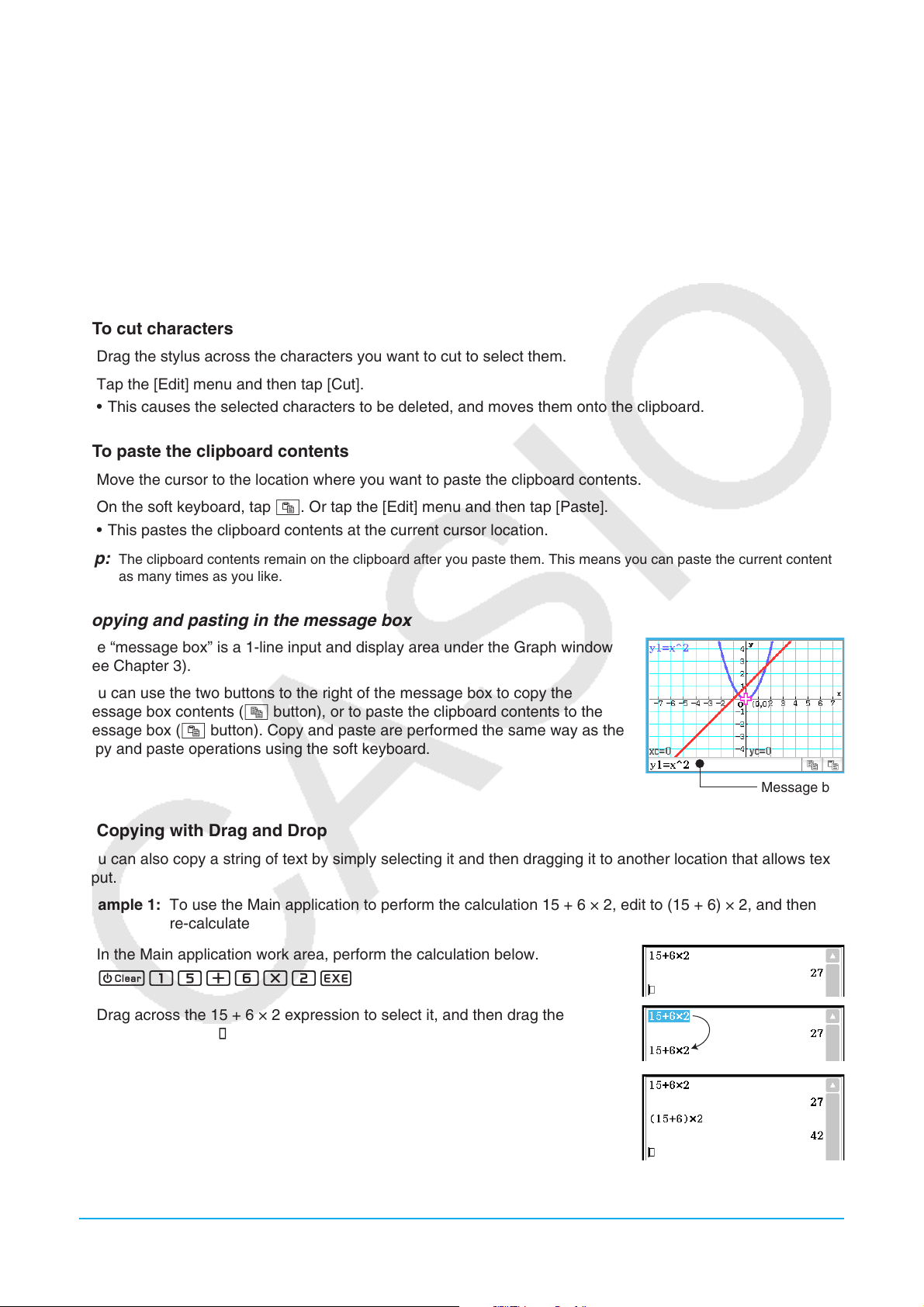
Copying and pasting in the message box
The “message box” is a 1-line input and display area under the Graph window
(see Chapter 3).
You can use the two buttons to the right of the message box to copy the
message box contents (p button), or to paste the clipboard contents to the
message box (q button). Copy and paste are performed the same way as the
copy and paste operations using the soft keyboard.
Message box
kCopying with Drag and Drop
You can also copy a string of text by simply selecting it and then dragging it to another location that allows text
input.
Example 1: To use the Main application to perform the calculation 15 + 6 × 2, edit to (15 + 6) × 2, and then
re-calculate
1. In the Main application work area, perform the calculation below.
c15+6*2E
2. Drag across the 15 + 6 × 2 expression to select it, and then drag the
expression to the .
• This will copy 15 + 6 × 2 to the location where you dropped it.
3. Add parentheses before and after 15 + 6 and then press E.
Tip: You can use drag and drop to copy both input formulas and calculation results.
Chapter 1: Basics 19
Page 20
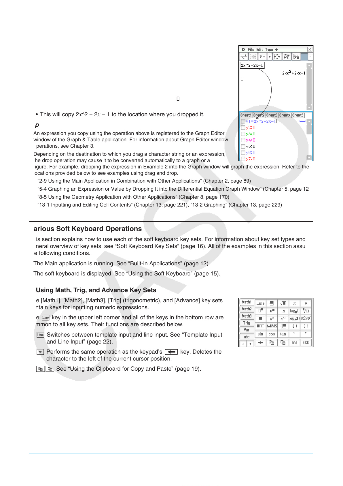
Example 2: To copy an expression you input with the Main application to the Graph Editor window
1. In the Main application work area, input: 2
x^2 + 2x − 1.
c2x{2+2x-1E
2. On the right end of the toolbar, tap the down arrow button. On the button
palette that appears, tap !.
• This will display the Graph Editor window in the bottom half of the screen.
3. Select the 2
x^2 + 2x − 1 expression you input with the Main application by
dragging across it, and then drag the expression to the located to the right
of y1: on the Graph Editor window.
• This will copy 2
x^2 + 2x − 1 to the location where you dropped it.
Tip
• An expression you copy using the operation above is registered to the Graph Editor
window of the Graph & Table application. For information about Graph Editor window
operations, see Chapter 3.
• Depending on the destination to which you drag a character string or an expression,
the drop operation may cause it to be converted automatically to a graph or a
figure. For example, dropping the expression in Example 2 into the Graph window will graph the expression. Refer to the
locations provided below to see examples using drag and drop.
- “2-9 Using the Main Application in Combination with Other Applications” (Chapter 2, page 89)
- “5-4 Graphing an Expression or Value by Dropping It into the Differential Equation Graph Window” (Chapter 5, page 124)
- “8-5 Using the Geometry Application with Other Applications” (Chapter 8, page 170)
- “13-1 Inputting and Editing Cell Contents” (Chapter 13, page 221), “13-2 Graphing” (Chapter 13, page 229)
Various Soft Keyboard Operations
This section explains how to use each of the soft keyboard key sets. For information about key set types and a
general overview of key sets, see “Soft Keyboard Key Sets” (page 16). All of the examples in this section assume
the following conditions.
• The Main application is running. See “Built-in Applications” (page 12).
• The soft keyboard is displayed. See “Using the Soft Keyboard” (page 15).
k Using Math, Trig, and Advance Key Sets
The [Math1], [Math2], [Math3], [Trig] (trigonometric), and [Advance] key sets
contain keys for inputting numeric expressions.
The L key in the upper left corner and all of the keys in the bottom row are
common to all key sets. Their functions are described below.
L Switches between template input and line input. See “Template Input
and Line Input” (page 22).
h Performs the same operation as the keypad’s K key. Deletes the
character to the left of the current cursor position.
pq See “Using the Clipboard for Copy and Paste” (page 19).
D Inputs “ans”. See “Using the Answer Variable (ans)” (page 43).
w Performs the same operation as the keypad’s E key, which executes calculations.
Chapter 1: Basics 20
Page 21
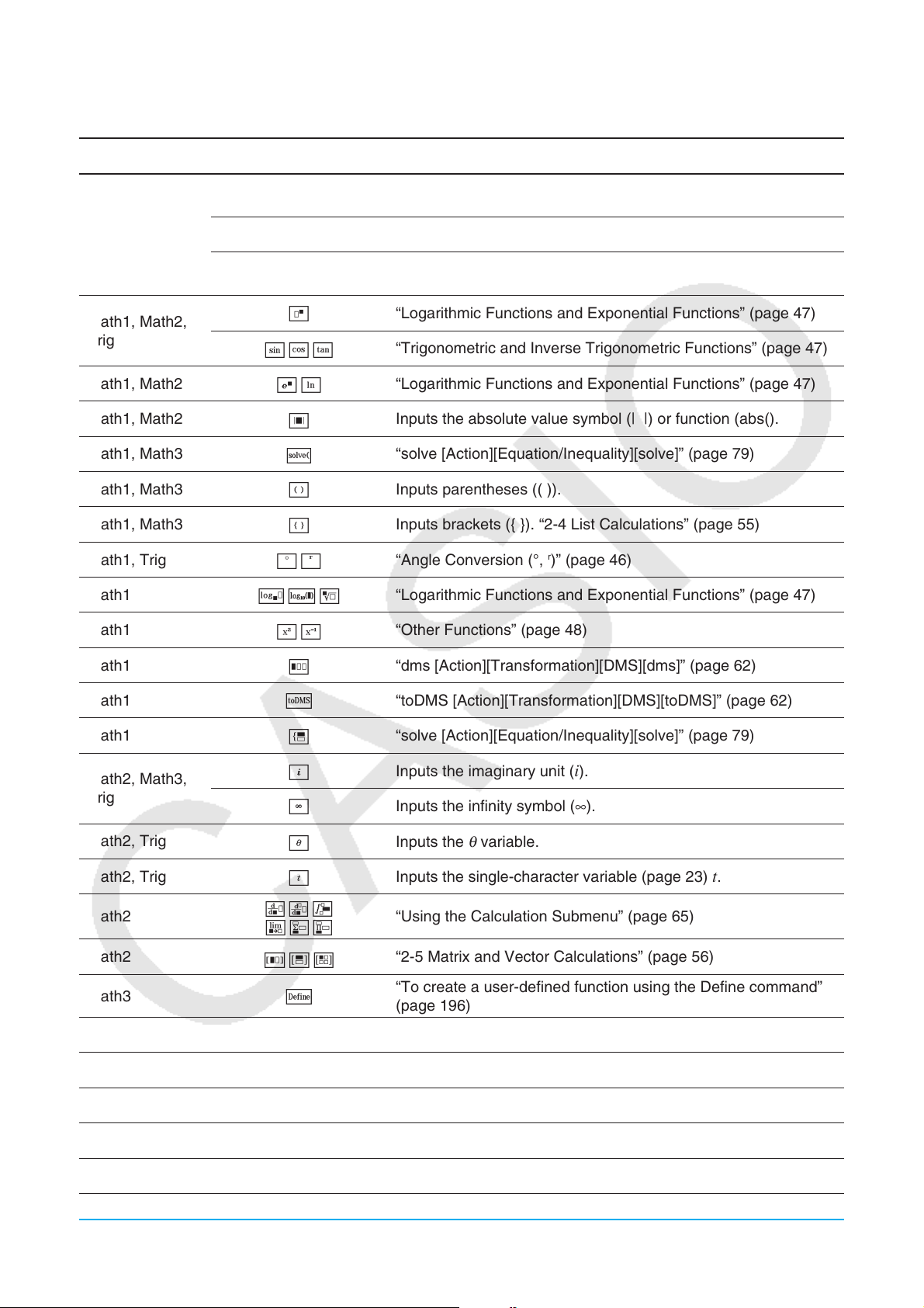
The keys in the following table are found on different key sets and are used to input functions and commands
for performing particular calculations and operations.
Key set Key Description
Math1, Math2,
Math3, Trig
Math1, Math2,
Trig
Math1, Math2
Math1, Math2
Math1, Math3
Math1, Math3
Math1, Math3
Math1, Trig
Math1
Math1
N5
p
W
m
sct
QI
4
.
(
)
*R
V"%
wE
“Template Input and Line Input” (page 22), “Other Functions”
(page 48)
Inputs pi (π).
Inputs the substitution symbol (⇒). “Creating a New Variable”
(page 31)
“Logarithmic Functions and Exponential Functions” (page 47)
“Trigonometric and Inverse Trigonometric Functions” (page 47)
“Logarithmic Functions and Exponential Functions” (page 47)
Inputs the absolute value symbol (| |) or function (abs().
“solve [Action][Equation/Inequality][solve]” (page 79)
Inputs parentheses (( )).
Inputs brackets ({ }). “2-4 List Calculations” (page 55)
r
“Angle Conversion (°,
)” (page 46)
“Logarithmic Functions and Exponential Functions” (page 47)
“Other Functions” (page 48)
Math1
Math1
Math1
Math2, Math3,
Trig
Math2, Trig
Math2, Trig
Math2
Math2
Math3
Math3
Math3
Math3
/
a
#
i
e
8
[
`*7
]_)
678
d
fg
'
+
“dms [Action][Transformation][DMS][dms]” (page 62)
“toDMS [Action][Transformation][DMS][toDMS]” (page 62)
“solve [Action][Equation/Inequality][solve]” (page 79)
Inputs the imaginary unit (
i).
Inputs the infinity symbol (∞).
θ
Inputs the
Inputs the single-character variable (page 23)
variable.
t.
“Using the Calculation Submenu” (page 65)
“2-5 Matrix and Vector Calculations” (page 56)
“To create a user-defined function using the Define command”
(page 196)
Inputs the “f” of f(
x), or the “g” of g(x).
“Derivative Symbol (’)” (page 52)
“dSolve [Action][Equation/Inequality][dSolve]” (page 80)
Math3
Math3
1
U
“piecewise Function” (page 52)
“with Operator ( | )” (page 53)
Chapter 1: Basics 21
Page 22
Key set Key Description
Math3
Math3
Math3
Trig
Trig
Advance
Advance
Advance
Advance
Advance
Advance
Advance
[
<>;:=/
~
SCT
123
!@#
:!
PN
NM<
hin
r
5%(^
7
6
Inputs square brackets ([ ]). “2-5 Matrix and Vector Calculations”
(page 56)
“Equal Symbols and Unequal Symbols” (page 53)
“Angle Symbol (∠)” (page 52)
“Trigonometric and Inverse Trigonometric Functions” (page 47)
“Hyperbolic and Inverse Hyperbolic Functions” (page 47)
“Other Functions” (page 48)
“Permutation (
“Chapter 6: Sequence Application”
“About rSolve” (page 127)
“Using the Advanced Submenu” (page 62)
“Gamma Function” (page 55)
“Dirac Delta Function” (page 54)
nPr) and Combination (nCr)” (page 51)
Advance
Advance
l
'
nth Delta Function” (page 54)
“
“Heaviside Unit Step Function” (page 54)
k Template Input and Line Input
ClassPad supports two different input methods: template input and line input. Template input lets you input
fractions, powers, and other functions using formats that are the same as those in textbooks. Line input uses a
linear format for inputting expressions.
2
2'2
2+
( )
'
Template Input Line Input
2+ 1
2+ (2 (2) / ( (2) + 1))^2
u Switching between Template Input and Line Input
Tap the L key. Each toggles the key color between white (L) and light blue ( ).
A white key indicates the template input mode, while a light blue key indicates the line input mode.
In the template input mode, you can perform template input using keys with
such as N and !. Other keys input the same functions or commands as they do in the line mode.
2
2'2
Example 1: To use the template input mode to input
1. Tap the [Math1] tab and then enter the template input mode (white L key).
2+
( )
'
2+ 1
or marked on their key tops,
2. Perform the key operation below:
2+(N2!2c!2e+1
eem2E
Chapter 1: Basics 22
Page 23
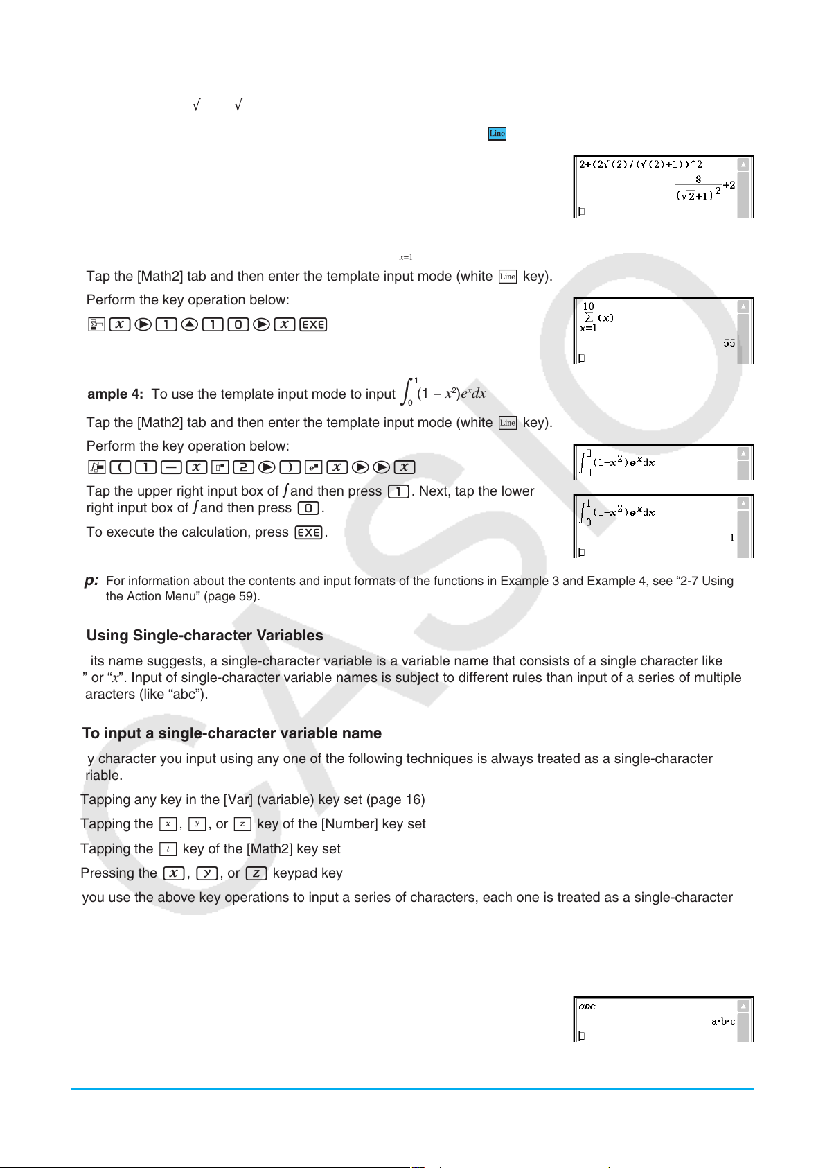
Example 2: To use the line input mode to input the same expression as in Example 1
∫
∫
(
2+ (2 (2) / ( (2) + 1))^2
)
1. Tap the [Math1] tab and then enter the line input mode (light blue
key).
2. Perform the key operation below:
2+(d2!2)N
(!2)+1)ewE
Example 3: To use the template input mode to input
Y
()
1. Tap the [Math2] tab and then enter the template input mode (white L key).
2. Perform the key operation below:
Oxe1f10exE
Example 4: To use the template input mode to input
1
(1 − 2)
∫
0
1. Tap the [Math2] tab and then enter the template input mode (white L key).
2. Perform the key operation below:
7(1-xm2e)Qxeex
3. Tap the upper right input box of
right input box of
and then press 0.
and then press 1. Next, tap the lower
4. To execute the calculation, press E.
Tip: For information about the contents and input formats of the functions in Example 3 and Example 4, see “2-7 Using
the Action Menu” (page 59).
k Using Single-character Variables
As its name suggests, a single-character variable is a variable name that consists of a single character like
“a” or “x”. Input of single-character variable names is subject to different rules than input of a series of multiple
characters (like “abc”).
u To input a single-character variable name
Any character you input using any one of the following techniques is always treated as a single-character
variable.
• Tapping any key in the [Var] (variable) key set (page 16)
• Tapping the X, Y, or Z key of the [Number] key set
• Tapping the [ key of the [Math2] key set
• Pressing the x, y, or Z keypad key
If you use the above key operations to input a series of characters, each one is treated as a single-character
variable. Inputting A, B, C using the [Var] key set, for example, is treated as the mathematical expression
a × b × c, and not as the characters “abc”.
Tip: The single-character variables described above make it possible for you to perform calculations as they appear in
your textbook.
Example 1: ABCw
Chapter 1: Basics 23
Page 24
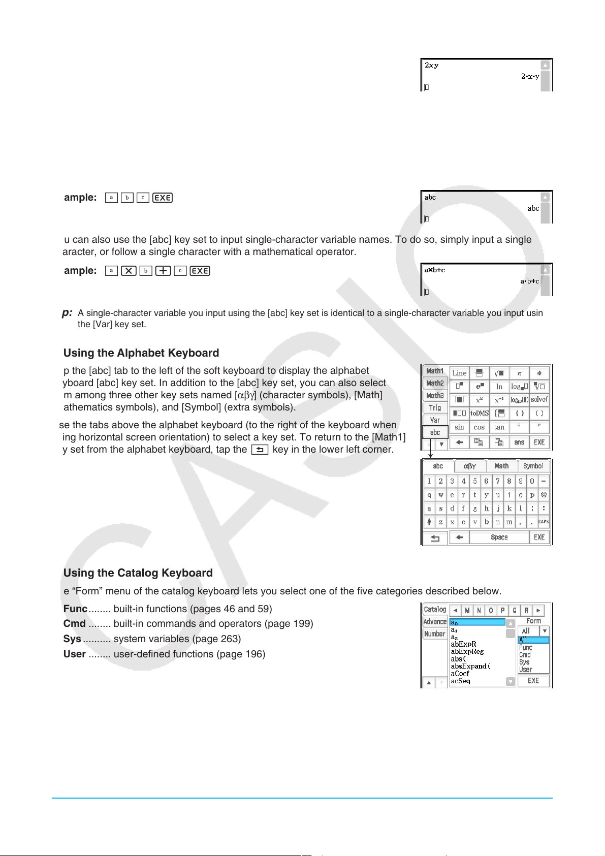
Example 2: 2xyE
Tip: When you input a single-character variable, its name appears on the display as an italicized character. This is simply
to let you know that the letter is a single-character variable name.
u To input a series of multiple characters
A series of multiple characters (like “list1”) can be used for variable names, program commands, comment text,
etc. Always use the [abc] key set when you want to input a series of characters.
Example: abcE
You can also use the [abc] key set to input single-character variable names. To do so, simply input a single
character, or follow a single character with a mathematical operator.
Example: a*b+cE
Tip: A single-character variable you input using the [abc] key set is identical to a single-character variable you input using
the [Var] key set.
k Using the Alphabet Keyboard
Tap the [abc] tab to the left of the soft keyboard to display the alphabet
keyboard [abc] key set. In addition to the [abc] key set, you can also select
from among three other key sets named [αβγ] (character symbols), [Math]
(mathematics symbols), and [Symbol] (extra symbols).
Use the tabs above the alphabet keyboard (to the right of the keyboard when
using horizontal screen orientation) to select a key set. To return to the [Math1]
key set from the alphabet keyboard, tap the I key in the lower left corner.
k Using the Catalog Keyboard
The “Form” menu of the catalog keyboard lets you select one of the five categories described below.
Func ........ built-in functions (pages 46 and 59)
Cmd ........ built-in commands and operators (page 199)
Sys .......... system variables (page 263)
User ........ user-defined functions (page 196)
All ............ all commands, functions, etc.
After selecting a category, you can choose the item you want from the alphabetized list that appears on the
catalog keyboard.
Tip: Note that user-defined variables and user-defined programs cannot be input using the catalog keyboard. Use
Variable Manager (page 27) instead.
Chapter 1: Basics 24
Page 25
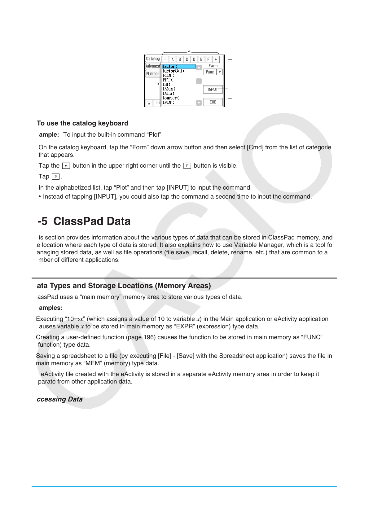
Catalog keyboard configuration
Tapping a letter button displays the
commands, functions, or other items that
begin with that letter.
This is an alphabetized list of commands,
functions, and other items available in the
category currently selected with “Form”.
Tap the down arrow button and then
select the category you want ([Func],
[Cmd], [Sys], [User], or [All]) from the list
that appears.
Tap this key to input the item that is
currently selected in the alphabetized list.
u To use the catalog keyboard
Example: To input the built-in command “Plot”
1. On the catalog keyboard, tap the “Form” down arrow button and then select [Cmd] from the list of categories
that appears.
2. Tap the + button in the upper right corner until the P button is visible.
3. Tap P.
4. In the alphabetized list, tap “Plot” and then tap [INPUT] to input the command.
• Instead of tapping [INPUT], you could also tap the command a second time to input the command.
1-5 ClassPad Data
This section provides information about the various types of data that can be stored in ClassPad memory, and
the location where each type of data is stored. It also explains how to use Variable Manager, which is a tool for
managing stored data, as well as file operations (file save, recall, delete, rename, etc.) that are common to a
number of different applications.
Data Types and Storage Locations (Memory Areas)
ClassPad uses a “main memory” memory area to store various types of data.
Examples:
• Executing “10⇒
causes variable x to be stored in main memory as “EXPR” (expression) type data.
• Creating a user-defined function (page 196) causes the function to be stored in main memory as “FUNC”
(function) type data.
• Saving a spreadsheet to a file (by executing [File] - [Save] with the Spreadsheet application) saves the file in
main memory as “MEM” (memory) type data.
An eActivity file created with the eActivity is stored in a separate eActivity memory area in order to keep it
separate from other application data.
Accessing Data
Besides the application that originally created it, data in main memory can also be accessed by any other
application. It can also be deleted, renamed, copied, moved and otherwise accessed using Variable Manager
(page 27). eActivity files can be accessed from the eActivity application only.
x” (which assigns a value of 10 to variable x) in the Main application or eActivity application
Chapter 1: Basics 25
Page 26

Main Memory Data Types
Data stored in main memory has a data type attribute that is assigned in accordance with the application that
created the data and the actual content of the data. The data type is indicated by a data type name. Data type
names are shown on the Variable Manager variable list, and on the Select Data dialog box that appears when
you are specifying a variable in any ClassPad application. The following table lists all of the data type names
and explains the meaning of each.
Data Type Name Data Type
EXPR Real number, complex number or expression data
STR String data
LIST List data created using the Statistics application, Main application, etc.
MAT Matrix data created using the Main application, etc.
PRGM* General program
EXE* Edit prohibited program
TEXT* Text data
FUNC* User-defined function
GMEM* Graph memory data saved using the Graph & Table application
For more information, see “Saving Graph Editor Data to Graph Memory” (page 100).
GEO* Geometry application data
MEM* Data saved to a file using one of the following applications: Spreadsheet, Geometry,
Verify (page 92), Probability (page 92).
OTHR Data other than that described above
Protected variable types
Some data types are protected. A variable whose data type is protected cannot be overwritten with another
variable, which protects variable contents from being inadvertently altered. Data types whose names are
marked with an asterisk in the above table are protected. Note that whether or not a data type is protected is
determined by the system. You cannot change the protection status of a data type.
Tip: Even when a variable is a protected data type, you can rename, delete, or move it. To disable these operations, you
need to lock the variable. See “Variable Manager operations” on page 27.
Main Memory Folders
Your ClassPad stores data in one of the following types of folders described below.
“main” folder: The “main” folder is a ClassPad reserved folder, and acts as the default current folder (see
“Current Folder” below).
“library” folder: Also a ClassPad reserved folder, the “library” folder can be used for storing user-created data
(variables, programs, user functions, etc.). Data stored in the “library” folder can be accessed without specifying
a path, regardless of the current folder setting.
User folder: This is a folder created and named by you. You can make a user folder the current folder, move
data to a user folder, etc. You can also delete and rename a user folder as required. You can have up to 87
user folders in main memory at one time.
Tip: You cannot put a folder inside of another folder.
Current Folder
The current folder is the folder where the data (excluding eActivity files) created by applications are stored
and from which such data can be accessed. The initial default current folder is the “main” folder. You can also
select a user folder you created as the current folder. For more information about how to do this, see “Variable
Manager operations” on page 27.
Chapter 1: Basics 26
Page 27
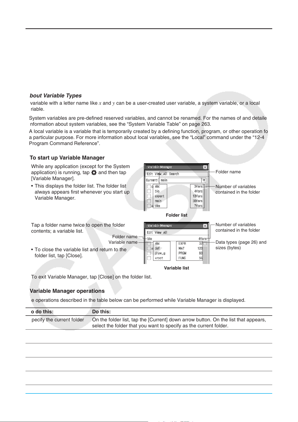
Using Variable Manager
Variable Manager is a tool for managing user variables, programs, user functions, and other types of data.
Though this section uses only the term “variables”, the explanations provided here also refer to the other types
of data that can be managed by Variable Manager.
With Variable Manager you can:
• Create, delete, rename, lock, and unlock folders, and configure current folder settings.
• Delete, copy, rename, move, lock, unlock, search for variables, and view the contents of variables.
About Variable Types
A variable with a letter name like x and y can be a user-created user variable, a system variable, or a local
variable.
• System variables are pre-defined reserved variables, and cannot be renamed. For the names of and detailed
information about system variables, see the “System Variable Table” on page 263.
• A local variable is a variable that is temporarily created by a defining function, program, or other operation for
a particular purpose. For more information about local variables, see the “Local” command under the “12-4
Program Command Reference”.
u To start up Variable Manager
1. While any application (except for the System
application) is running, tap O and then tap
[Variable Manager].
• This displays the folder list. The folder list
always appears first whenever you start up
Variable Manager.
Folder name
Number of variables
contained in the folder
Folder list
2. Tap a folder name twice to open the folder
contents; a variable list.
Folder name
Variable name
• To close the variable list and return to the
Number of variables
contained in the folder
Data types (page 26) and
sizes (bytes)
folder list, tap [Close].
Variable list
3. To exit Variable Manager, tap [Close] on the folder list.
u Variable Manager operations
The operations described in the table below can be performed while Variable Manager is displayed.
To do this: Do this:
Specify the current folder On the folder list, tap the [Current] down arrow button. On the list that appears,
select the folder that you want to specify as the current folder.
Create a folder On the folder list, tap [Edit] - [Create Folder]. On the dialog box that appears,
enter the name you want to assign to the folder and then tap [OK].
Open a folder On the folder list, tap the name of the folder you want to open so it is
highlighted, and then tap it again.
Open the “library” folder Tap [View] and then [“library” Folder]. This opens the “library” folder and
displays a variable list showing its contents.
Select a folder or variable Select the check box next to the folder or variable name. To select all the
folders or variables in the list, tap [All] and then [Select All].
Chapter 1: Basics 27
Page 28
To do this: Do this:
Deselect a folder or
variable
Delete a folder See “To delete a folder” (page 29).
Delete a variable Select the check box next to the variable you want to delete, and then tap [Edit]
Rename a folder or
variable
Lock a folder or variable Select the check box next to the folder or variable you want to lock, and then
Unlock a folder or variable Select the check box next to the folder or variable you want to unlock, and then
Display a list of a
particular type of variable
Copy or move a variable On the variable list, tap [Edit] and then [Copy] or [Move]. On the dialog box that
Clear the check box next to the folder or variable name. To deselect all the
folders or variables in the list, tap [All] and then [Deselect All].
- [Delete]. In response to the confirmation dialog box that appears, tap [OK] to
delete the selected variable.
Highlight the folder or variable you want to rename and then tap [File] [Rename]. On the dialog box that appears, enter the name you want to assign
to it and then tap [OK].
tap [Edit] - [Lock]. This locks the currently selected folder or variable, and adds
a b icon to the left of its name to indicate that it is locked.
tap [Edit] - [Unlock].
On the variable list, tap [View] - [Variable Type]. On the dialog box that appears,
tap the down arrow button and then select the data type from the list that
appears and then tap [OK].
appears, tap the down arrow button and then select the destination folder from
the list that appears and then tap [OK].
Tip
• If a variable with the same name already exists in the destination folder, the variable in
the destination folder is replaced with the one that you are copying or moving.
• A variable that is locked cannot be moved.
View the contents of a
variable
Input a folder name or
variable name into an
application
Search for a variable On the folder list, tap [Search]. On the dialog box that appears, enter the
On the variable list, tap the name of the variable whose contents you want to
view so it is highlighted, and then tap it again. This displays a dialog box that
shows the contents of the variable.
See “To input a folder name or variable name into an application” (page 29).
variable name you want to find and then tap [OK].
An exclamation point (!) appears in front of all folders containing a variable
name that matches the name in your search.
Note: You can use the above procedure to search the “main” folder or a user
defined folder for a particular variable name. Note that you cannot search the
“library” folder.
Selecting a Folder
• If no check box is selected on the folder list, any folder operation that is performed affects the folder whose
name is currently highlighted on the list. If any folder check box is selected, only that folder is affected by a
folder operation, and the folder whose name is highlighted on the list is not affected.
• Selecting the check box of a folder causes the check boxes of all of the variables inside of it also to become
selected.
• When renaming a folder, only the folder whose name is highlighted on the folder list is renamed. Other folders
whose check boxes are selected are not affected.
Chapter 1: Basics 28
Page 29
Selecting a Variable
• If no check box is selected on the variable list, any variable operation that is performed affects the variable
whose name is currently highlighted on the list. If any variable check box is selected, only that variable is
affected by a variable operation, and the variable whose name is highlighted on the list is not affected.
• When renaming a variable, only the variable whose name is highlighted on the variable list is renamed. If
other variables are selected (checked), they will not be affected.
Folder and Variable Name Rules
The following are the rules that apply to folder and variable names.
• Folder or variable names can be up to 8 bytes long.
• The following characters are allowed in a folder or variable name: Upper-case and lower-case characters,
subscript characters, numbers, underscore (_).
• Folder or variable names are case-sensitive. For example, each of the following is treated as a different
folder/variable name: abc, Abc, aBc, ABC.
• A reserved word (system variable names, built-in function names, command names, etc.) cannot be used as
a folder or variable name.
• A number, subscript characters or the underscore (_) cannot be used as the first character of a folder or
variable name.
u To delete a folder
Important!
Before deleting a folder, make sure you no longer need any of the variables contained inside it. It is probably
a good idea to first delete the variables you don’t need, move the variables you do need to another folder, and
then delete the empty folder.
1. Open the folder you want to delete and check its contents.
• Make sure you no longer need any of the variables in the folder. If any of the variables are locked, unlock
them.
• After checking the contents of the folder, close it to return to the folder list.
2. Select the check box next to the folder you want to delete.
• You can select and delete multiple folders, if you want.
3. On the folder list, tap [Edit] and then [Delete].
4. In response to the confirmation dialog box that appears, tap [OK] to delete the folder.
Tip: You cannot delete the “library” folder or the “main” folder.
u To input a folder name or variable name into an application
1. In the Main application, Graph & Table application, or some other application, move the cursor to the location
where you want to input the variable name.
2. Start up Variable Manager to display the folder list.
3. If you want to input a variable name, double-tap the folder that includes the variable whose name you want to
input. If you want to input a folder name, advance to the next step.
4. Tap the folder or variable whose name you want to input, so its name is highlighted.
5. Tap [INPUT].
• This exits Variable Manager and inputs the name of the folder or variable you selected in step 4 into the
application at the current cursor position.
Chapter 1: Basics 29
Page 30
Managing Application Files
The applications below can save data to files.
Geometry (Chapter 8), eActivity (Chapter 10), Spreadsheet (Chapter 13), Verify (page 92), Probability (page 92)
This section explains the common operations that can be performed on data files created with these
applications.
Tip: The eActivity file save dialog box is slightly different from the save dialog box of the other applications, but operations
are basically the same.
u To save a file
1. Tap [File] and then [Save].
2. On the dialog box that appears, tap the name of the folder where you want to save the file so it is selected.
3. Input up to 8 bytes for the file name in the file name edit box, and then tap [Save].
u To open an existing file
1. Tap [File] and then [Open].
2. On the dialog box that appears, open the folder that contains the file you want to open.
3. Tap the name of the file you want to open so it is selected, and then tap [Open].
u To search for a file
1. Tap [File] and then [Open].
2. On the dialog box that appears, tap [Search]. This displays the Search dialog box.
3. Enter the file name you want to find and then tap [Search].
• File names that match the one you enter become highlighted on the display. Tapping [Open] opens the
highlighted file.
• To search for the next occurrence of the file name, tap [Search] again and then tap [Next] on the Search
dialog box.
u To delete a folder or file
Important!
Deleting a folder also deletes all files inside of it. Please double-check to make sure you no longer need the
contents of a folder before deleting it.
1. Tap [File] and then [Open].
2. On the dialog box that appears, select the check box next to the folder or file you want to delete.
• You can select multiple folders/files for deletion, if you want.
• Selecting a check box next to a folder name automatically checks the boxes for all files inside that folder.
3. Tap [File] and then [Delete].
4. In response to the confirmation dialog box that appears, tap [OK] to delete the folder(s) or file(s).
Tip: Selecting a folder in the above procedure deletes the folder and all of its contents. Note, however, that the “main”
folder cannot be deleted, even if you check it.
u To rename a folder or file
1. Tap [File] and then [Open].
2. On the dialog box that appears, tap the name of the folder or file you want to rename so it is selected.
3. Tap [File] and then [Rename]. This displays the Rename dialog box.
4. Enter the name you want to assign to it and then tap [OK].
Chapter 1: Basics 30
Page 31

u To move a file to another folder
1. Tap [File] and then [Open].
2. On the dialog box that appears, select the check box next to the file you want to move.
• To move multiple files, select all of their check boxes.
3. Tap [File] and then [Move].
• This causes a dialog box for selecting the destination folder to appear.
4. On the dialog box, tap the down arrow button and then select the destination folder from the list that appears.
5. Tap [OK] to move the files.
u To switch the file menu view between List View and Detail View (eActivity application only)
1. Tap [File] and then [Open].
2. On the dialog box that appears, open the folder that contains the files you want to list.
3. To display both the file name and file size, tap [View] - [Detail View]. To display file names only, tap [View] -
[List View].
u To create a new folder
1. Tap [File] and then [Open].
2. On the dialog box that appears, tap [File] and then [Create Folder], or tap {.
• This displays the Create Folder dialog box.
3. Enter up to 8 bytes for the folder name, and then tap [OK] to create a folder.
1-6 Creating and Using Variables
This section explains how to create a new variable (user variable), and provides a simple sample calculation
that illustrates how to use a variable.
Creating a New Variable
The most common way to create a new variable is assigning a value or expression to the applicable variable
name. Use the variable assignment key (W) to assign data to a variable.
The following is an example of assignment to a variable while “main” is specified as the current folder.
Example: To create a new variable named “eq1” and assign the expression 2
The following assumes that there are no variables named “eq1” or “x” currently in the “main” folder.
u ClassPad Operation
1. Start the Main application.
2. Press k to display the soft keyboard, and then perform the following key operation.
2x+11W0eqbw
x + 1 to it
• This creates a variable named “eq1” in the current folder (the “main” folder
in this example), and assigns the expression 2
x + 1 to it.
Chapter 1: Basics 31
Page 32

Tip
• If a variable with the specified name already exists in the current folder, the contents of the existing variable are replaced
with the newly assigned data, unless the existing variable is locked or protected. For more information, see “Variable
Manager operations” (page 27) and “Protected variable types” (page 26).
• To store the newly created variable in a folder other than the current folder, specify the variable name as follows:
<folder name>\<variable name>.
• You can use Variable Manager to view the contents of a variable you create. For more information, see “Variable Manager
operations” (page 27).
• For information about rules for naming variables, see “Folder and Variable Name Rules” (page 29).
Variable Usage Example
The following example uses the variable we created in the example under “Creating a New Variable” above.
Example: To assign values of 5 and 10 to
x and check the results of eq1 (= 2x + 1)
u ClassPad Operation
1. Assign 5 to x.
51WxE
2. Check the contents of variable “eq1”.
0eqbw
• This displays the calculation result of 2
3. Assign 10 to
101WxE
4. Check the contents of variable “eq1”.
0eqbw
x.
x + 1 when x = 5.
“library” Folder Variables
Variables in the “library” folder can be accessed without specifying a path name, regardless of the current
folder.
Example: To create and access two variables, one located in the “library” folder and one located in another
folder
u ClassPad Operation
1. With “main” specified as the current folder, perform the following operation to create a variable named “eq1”
and assign the indicated list data to it.
{1, 2, 3} W eq1w
2. Keeping “main” specified as the current folder, perform the following operation to create a variable named
“eq2” in the “library” folder, and assign the indicated list data to it.
{4, 5, 6} W library\eq2w
3. Check the contents of the two variables.
eq1w
eq2w
(Since variable “eq2” is stored in the “library” folder, you do not need to
indicate a path to access it.)
Chapter 1: Basics 32
Page 33

4. Change the current folder specification to “Test”.
• Use Variable Manager (page 27) to create a folder named “Test” and change the current folder specification.
5. Perform the following operations to view the contents of variables “eq1” and “eq2”.
eq1E
(Since this key operation does not access the “main” folder, the variable
name (“eq1”) is displayed without showing the variable contents.)
main\eq1E
(Specifying the path to the “main” folder where “eq1” is located displays
the contents of the variable.)
eq2E
(Since variable “eq2” is stored in the “library” folder, you do not need to
indicate a path to access it.)
Tip: Specifying a variable name that exists in both the current folder and the “library” folder causes the variable in the
current folder to be accessed. For details about the variable access priority sequence and how to access variables in
particular folders, see “Rules Governing Variable Access” below.
Rules Governing Variable Access
Normally, you access a variable by specifying its variable name. The rules in this section apply when you need
to reference a variable that is not located in the current folder or to access a variable that has the same name
as one or more variables located in other folders.
kVariable Search Priority Sequence
Specifying a variable name to access a variable causes variables to be searched in the sequence below.
(1) Local variables (2) Current folder variables (3) “library” folder variables
• Multiple variables with the same name can exist simultaneously as a local variable, as a variable in the
current folder, and as a variable in the “library” folder. In this case, the ClassPad searches folders according
to the sequence shown above and accesses the first instance of the variable that it finds. If you want to
access such a variable when it occurs lower in the above sequence, you need to specify the folder name
along with the variable name as shown in “Specifying a Variable in a Particular Folder” below.
• If a variable you specify cannot be found, it is treated as an “undefined variable”.
• Note that “system” variables are not included in the above variable search. When accessing a system
variable, you need to specify the variable name only, without specifying the folder name.
Tip: Only local variables and current folder variables are searched in the case of an operation that stores variable data
or a command that performs an operation on a variable (like “DelVar”). Normally, “library” folder variables are not
searched. If you want to include “library” folders in the search, you need to specify the “library” folder as the variable
location as explained below.
kSpecifying a Variable in a Particular Folder
You can access a variable located inside the “main” folder, “library” folder, or a particular user folder by
specifying the folder name along with the variable name.
Use the following syntax when specifying a folder name:
<folder name>\<variable name>
Example: To specify variable “abc” located in the “main” folder
main\abc
Chapter 1: Basics 33
Page 34

1-7 Configuring Application Format Settings
The O menu includes format settings for configuring the number of calculation result display digits and
the angle unit, as well as application-specific commands. The following describes each of the settings and
commands that are available on the O menu.
To do this:
Specify folder for variables, and to configure number format, angle, and other basic
settings for all built-in applications
Configure Graph window and graph drawing settings for Graph & Table, Conics, and
other graphing applications
Configure number format, angle, and other settings for Geometry application Geometry Format
Configure Fourier transform and FFT settings Advanced Format
Configure Financial application settings Financial Format
Return all the above menu settings to their initial default values (except for the current
folder setting specified on Basic Format dialog box)
Select this O
menu command:
Basic Format
Graph Format
Default Setup
u To configure application format settings
1. Open any application (except the System application).
2. Tap O. Next, tap the menu command you want: Basic Format, Graph Format, Geometry Format, Advanced
Format, or Financial Format.
3. Use the dialog box to configure the settings you want.
• For details about the settings you can configure on each of the dialog boxes, see “Application Format
Settings” below.
4. To close a dialog box and apply its settings, tap [Set]. To close a dialog box without applying its settings, tap
[Cancel] or the C button in the upper right corner of the dialog box.
Application Format Settings
This section provides details about all of the settings you can configure using the application format settings.
Settings marked with an asterisk (*) in the following explanations are ClassPad initial default settings.
k Basic Format Dialog Box
Use the Basic Format dialog box to configure basic settings for calculations, cells, and other parameters.
To specify the current folder
Tap 1 and then tap the name of the folder (main*) you want.
1
To specify the numeric value display format
Tap 2 and then tap one of the settings described below.
2
Normal 1*: Automatically uses exponential display format when calculation
3
result
x is: 10
Normal 2: Automatically uses exponential display format when calculation
result
x is: 10
Fix 0 – Fix 9: Fixed number of decimal places
Sci 0 – Sci 9: Fixed number of significant digits
To specify the angle unit
Tap 3, and then tap “Radian*”, “Degree”, or “Grad”.
−2
> |x| or |x| t 1010.
−9
> |x| or |x| t 1010.
Chapter 1: Basics 34
Page 35

To do this: Do this:
Switch between complex number calculations
(Complex mode) and real number calculations (Real
mode)
Display results as a decimal value (Decimal mode)
or leave calculation results as expressions (Standard
mode)
Turn auto simplification of expressions on (Algebra
mode) or off (Assistant mode)
Select the “Complex Format” check box to enter the
Complex mode, or clear the check box* to enter the
Real mode*.
Select the “Decimal Calculation” check box to enter
the Decimal mode, or clear the check box* to enter
the Standard mode.
Select the “Assistant” check box to enter the
Assistant mode, or clear the check box* to enter the
Algebra mode. See page 44 for details.
Specify descending order or ascending order for the
calculation result expression
Select the “Descending Order” check box* to display
calculation result expressions in descending order
2
x
(like
ascending order (like 1 + x + x2).
Specify whether variables in Complex Mode
calculation should be treated as real numbers or
complex numbers
Select the “Variable is Real” check box to treat
variables as real numbers, or clear the check box* to
treat variables as complex numbers.
+ x + 1), or clear the check box to display in
Tip: For information about the “Q
1
, Q3 on Data” check box, see “Calculation Methods for Q1 and Q3” (page 136).
Using Status Bar to Change Application Format Settings
With the applications listed in the table below, you can use the status bar to check and modify a number of
Basic Format dialog box settings.
For this application: You can check and change these settings:
Main, eActivity Algebra mode/Assistant mode setting, Standard mode/Decimal mode
setting, Complex mode/Real mode setting, angle unit setting
Statistics Standard mode/Decimal mode setting, angle unit setting
Graph & Table, Conics,
Complex mode/Real mode setting, angle unit setting
Differential Equation Graph,
Numeric Solver, Sequence
u To use the status bar to change application format settings
On the status bar, tap the text of the setting you want to change.
Main application Graph & Table application
Each tap changes the tapped item as described below.
• “Alg” ↔ “Assist” ... Toggles between the Algebra mode and Assistant mode.
• “Standard” ↔ “Decimal” ... Toggles between the Standard mode and Decimal mode.
• “Real” ↔ “Cplx” ... Toggles between the Real mode and Complex mode.
• “Rad” → “Deg” → “Gra” ... Cycles the angle unit setting between Radian, Degree, and Grad.
Tip: Changing a setting using the status bar has the same effect as changing the corresponding setting on the Basic
Format dialog box. This means the setting will be changed for all applications.
Chapter 1: Basics 35
Page 36

k Graph Format Dialog Box
Use the Graph Format dialog box to configure settings for the Graph window and for drawing graphs.
[Basic] tab
To specify display of Graph window axes
Tap 1 and then tap one of the settings described below.
On: show axis Off: hide axis
1
Number*: show axis along with maximum and minimum value of each axis
2
To specify display of Graph window grid
Tap 2 and then tap one of the settings described below.
3
On: show grid as dots Off: hide grid
4
Line*: show grid as lines
To select inequality fill specification (Inequality Plot)
Tap 3 and then tap one of the settings described below.
Union*: fill areas where all inequality conditions are satisfied when
graphing multiple inequalities
Intersection: fill areas where each inequality condition is satisfied when
graphing multiple inequalities
To specify the color of figures and graphs drawn with the Sketch function (page 110)
Tap 4. On the dialog box that appears, select the color you want and then tap [OK].
To do this: Do this:
Turn display of Graph
window axis labels on
or off
Turn display of graph
controller arrows on
Select the “Labels” check box* to show labels, or clear the check box to hide
labels.
Tip: Regardless of the “Labels” setting, labels are never displayed on the Sequence
application Graph window. Also, labels are not displayed for the following types
of graph drawn with the Statistics application: NPPlot, Histogram, MedBox, NDist
Broken.
Select the “G-Controller” check box to show graph controller arrows (page 103), or
clear the check box* to hide graph controller arrows.
or off
Specify plotted points
or solid lines for graph
Select the “Draw Plot” check box to specify plotted points, or clear the check box*
to specify solid lines for graphing.
drawing
Turn display of the
function name and
Select the “Graph Function” check box* to show the function name and function on
the graph, or clear the check box to hide the function name and function.
function on or off
Turn display of Graph
window pointer
Select the “Coordinates” check box* to show Graph window pointer coordinates, or
clear the check box to hide the coordinates.
coordinates on or off
Turn display of the
leading cursor during
Select the “Leading Cursor” check box to show the leading cursor, or clear the
check box* to hide the leading cursor.
graphing on or off
Specify the draw
method when drawing
Select the “Simultaneous Graphs” check box to draw multiple graphs
simultaneously, or clear the check box* to draw graphs in sequence, one at a time.
multiple graphs
Show or hide
derivative values on
the Graph window and
Table window
Select the “Derivative/Slope” check box to show derivative values in the Graph
window and Table window, or clear the check box* to hide derivative values. For
details about display contents, see “Using Trace to Read Graph Coordinates”
(page 109) and “Generating a Number Table” (page 106).
Chapter 1: Basics 36
Page 37

[Special] tab
To specify the row width for Stat Editor and data table displays
Tap 1, and then select “2 Cells”, “3 Cells*”, or “4 Cells”.
To specify a source for table data
1
Tap 2 and then tap one of the settings described below.
2
Table Input*: Uses the data input in a Table Input dialog box as the source
for number table generation.
3
list1 through list6: Uses list data in list1 through list6 as the source for
number table generation.
<list name>: Uses the list data in a selected list as the source for number
table generation.
For details about how to generate a number table using each setting, see
“Generating a Number Table” (page 106).
To specify a source for summary table data
Tap 3 and then tap one of the settings described below.
View Window*: Uses View Window settings as the source for summary table generation.
list1 through list6: Uses list data in list1 through list6 as the source for summary table generation.
<list name>: Uses the list data in a selected list as the source for summary table generation.
For details about how to generate a summary table using each setting, see “Generating a Summary Table”
(page 108).
To show or hide the second derivative for summary tables
Select the On button* under “Summary Table
To specify auto setting or manual setting of Statistics application View Window settings
Select the “Stat Window Auto” check box* to specify automatic setting configuration, or clear the check box for
manual settings.
f (x)” to show the second derivative, or the Off button to hide it.
Chapter 1: Basics 37
Page 38

k Geometry Format Dialog Box
Use the Geometry Format dialog box to configure settings for the Geometry application.
Tip: The information that appears in the preview area at the bottom of the dialog box shows a preview of the Geometry
application window, based on the settings configured in upper part of the dialog box.
To specify the Geometry window numeric value display format
Tap 1 and then select the format you want. The initial default Number
1
Format setting is Fix2. For more information, see “To specify the numeric
value display format” (page 34).
2
To specify the unit of the displayed length value
3
Tap 2 and then tap one of the settings described below.
4
Off*: Length value unit not displayed.
mm, cm, m, km, in, ft, yd, mi: Displays the length value in the selected
5
6
To specify the initial status of Graph window axes when the Geometry application is started up
Tap 5 and then tap one of the settings described below.
On: Show the axes Off*: Hide the axes
Number: Show the axes along with the maximum and minimum value of each
unit.
To specify the angle unit for the measurement box
Tap 3, and then tap “Radian”, “Degree*”, or “Grad”.
To specify the angle unit for graphing
Tap 4, and then tap “Radian*”, “Degree”, or “Grad”.
To specify the initial status of the grid when the Geometry application is started up
Tap 6 and then tap one of the settings described below.
On: Show the grid as dots Off*: Hide the grid Line: Show the grid as lines
k Advanced Format Dialog Box
Use the Advanced Format dialog box to configure settings for Fourier transform and FFT settings.
To specify the Fourier transform formula
Tap 1 and then tap “Modern Physics”, “Pure Math*”, “Probability”,
“Classical Physics”, or “Signal Processing”.
1
To specify the FFT scaling constant
Tap 2 and then tap “Pure Math”, “Signal Processing*”, or “Data Analysis”.
To specify how Fourier calculation variables are treated
Select the “Assume positive real” check box* to specify that Fourier
calculation variables should be treated as positive reals only. Clear
the check box to specify that complex numbers are allowed for Fourier
2
calculation variables.
Chapter 1: Basics 38
Page 39

k Financial Format Dialog Box
Use the Financial Format dialog box to configure settings for the Financial application.
[Basic] tab
To specify the number of days in a year
Tap 1, and then tap “360 days” or “365 days*”.
To specify the beginning or the period or the end of the period as the
1
payment date
Tap 2 and then tap “Beginning of period” or “End of period*”.
2
To specify the date format
3
Tap 3 and then tap one of the settings described below.
MM/DD/YYYY*: month/day/year
DD/MM/YYYY: day/month/year
YYYY/MM/DD: year/month/day
To specify the status of input fields when starting a new calculation
To do this: Do this:
When changing to another calculation type,
automatically copy the contents of all fields in the
current calculation whose names match the names
of fields in the new calculation.
When changing to another calculation type, clear all
fields.
Select the [Automatically copy common fields to new
calculation] check box*.
Clear the [Automatically copy common fields to new
calculation] check box.
Chapter 1: Basics 39
Page 40

[Special] tab
To specify odd period handling
Tap 1 and then tap one of the settings described below.
Compound (CI): Apply compound interest to the odd period when
1
2
3
4
5
To specify whether to use the amount (PRF) or profit ratio (r%) when performing break-even point
calculations
Tap 4, and then tap “Amount (PRF)*” or “Ratio (r%)”.
To specify whether to calculate sales quantity ([QBE]) or sales amount ([SBE]) first when performing
break-even point calculations
Tap 5, and then tap “Quantity*” or “Sales”. When “Quantity” is selected, sales quantity can be calculated
before calculating the sales amount. When “Sales” is selected, sales amount can be calculated before
calculating the sales quantity.
performing a Compound Interest calculation
Simple (SI): Apply simple interest to the odd period when performing a
Compound Interest calculation
Off*: Apply no interest to the odd period when performing a Compound
Interest calculation
To specify the compounding frequency
Tap 2, and then tap “Annual*” (once a year) or “Semi-annual” (twice a
year).
To specify the bond interval
Tap 3 and then tap one of the settings described below.
Term*: Specifies use of the number of payments as the duration for bond
calculation.
Date: Specifies use of a date as the duration for bond calculation.
Tip: When performing a financial calculation, you can change settings using the Financial application status bar and
[Format] tab. For more information, see “Configuring Financial Application Settings” (page 181).
Initializing All Application Format Settings
Perform the following procedure when you want to return all application format settings to their initial defaults.
u ClassPad Operation
1. Tap O and then tap [Default Setup].
2. In response to the “Reset Setup Data?” message that appears, tap [OK] to initialize all settings.
• The settings are initialized except for the current folder setting specified on Basic Format dialog box.
Chapter 1: Basics 40
Page 41

1-8 When you keep having problems…
If you keep having problems when you are trying to perform operations, try the following before assuming that
there is something wrong with the ClassPad.
1. Initialize all application format settings.
Perform the procedure under “Initializing All Application Format Settings” (page 40).
2. Perform the RAM reset (RESTART) operation.
Perform RAM reset when the ClassPad freezes up or otherwise fails to perform as expected for some
reason.
To perform the RAM reset operation
Important!
• The RAM reset operation deletes all data that is temporarily stored in ClassPad RAM. Performing the RAM
reset operation while a calculation is in progress will cause any data stored in RAM by the calculation to be
lost.
• Perform the RAM reset operation only when your ClassPad freezes up or when it begins to operate
abnormally for some reason.
1. Use the stylus to press the RESTART button on the back of the
ClassPad.
• Following the RAM reset operation, the ClassPad restarts
automatically.
RESTART
Button
2. After the ClassPad restarts, perform the ClassPad setup operation. For more information about the
procedures you need to perform here, see “Replacing Batteries and Setting Up the ClassPad” in the
separate Quick Start Guide.
• The application menu appears after you finish the setup operation.
3. Reset the ClassPad.
Before performing the reset operation, first make a written copy of all important data.
For details, see “To batch delete specific data (Reset)” (page 245).
Chapter 1: Basics 41
Page 42
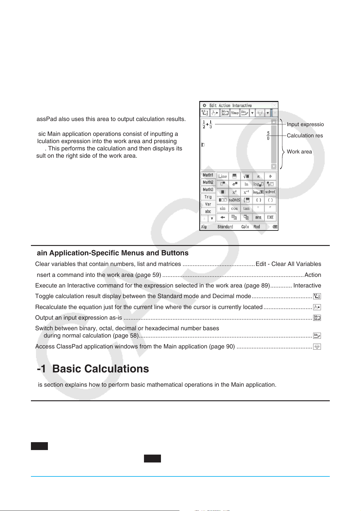
Chapter 2: Main Application
The Main application is a general-purpose numerical and mathematical calculation application that you can use
to study mathematics and solve mathematical problems. You can use the Main application to perform general
operations from basic arithmetic calculations, to calculations that involve lists, matrices, etc.
Starting up the Main application displays a large white work
area. Use this area for inputting operations and commands.
ClassPad also uses this area to output calculation results.
Basic Main application operations consist of inputting a
calculation expression into the work area and pressing
E. This performs the calculation and then displays its
result on the right side of the work area.
Input expression
Calculation result
Work area
Main Application-Specific Menus and Buttons
• Clear variables that contain numbers, list and matrices ...........................................Edit - Clear All Variables
• Insert a command into the work area (page 59) .................................................................................... Action
• Execute an Interactive command for the expression selected in the work area (page 89) ............. Interactive
• Toggle calculation result display between the Standard mode and Decimal mode ....................................u
• Recalculate the equation just for the current line where the cursor is currently located ............................. 7
• Output an input expression as-is ................................................................................................................0
• Switch between binary, octal, decimal or hexadecimal number bases
during normal calculation (page 58).......................................................................................................<
• Access ClassPad application windows from the Main application (page 90) .............................................$
2-1 Basic Calculations
This section explains how to perform basic mathematical operations in the Main application.
Arithmetic Calculations and Parentheses Calculations
You can perform arithmetic calculations by inputting expressions as they are written. The ClassPad
automatically judges the calculation priority sequence for addition, subtraction, multiplication, and division,
functions, and parentheses.
0201 Calculation examples
• All of the example calculations shown in
key set, unless noted otherwise.
0201 are performed using the keypad or the soft keyboard [Number]
Chapter 2: Main Application 42
Page 43

• The example calculations are all performed using the Decimal mode (see page 44).
Using the e Key
Use the e key to input exponential values. You can also input exponential values using the E key on the
soft keyboard [Number] key set.
0202 Calculation examples
Omitting the Multiplication Sign
You can omit the multiplication sign in any of the following cases.
• In front of a function… 2sin (30), 10log (1.2), etc.
• In front of a constant or variable… aπ, 2ab, 3ans, etc.
• In front of an open parenthesis… 3(5 + 6), (a + 1)(b – 1), etc.
Note that you must use a multiplication sign when the expression directly in front of the open parenthesis is a
literal variable. Example: ab (3 + b) must be written ab × (3 + b). Otherwise, your input is considered to be in
function notation (
• In front of the e key or E key (See “Using the e Key” above.)
• In front of a matrix or list… a {1, 2, 3}, 3 [[1, 2] [3, 4]], etc.
f ( x )).
Using the Answer Variable (ans)
Any time you execute a calculation in the Main application work area, the last result is assigned automatically
to a variable named “ans” (answer). You can even recall current “ans” variable contents and input them into
another calculation by tapping the D key on the soft keyboard.
0203 Calculation examples
Tip: Starting a calculation expression with +, −, ×, ÷, or ^ operator will cause the “ans” variable to be inserted automatically
to the left of the operator, even if you do not tap the D key.
Assigning a Value to a Variable
Besides using the variable assignment key (W, page 31), you can also use the syntax shown below in the Main
application and eActivity application to assign a value to a variable.
Syntax: Variable: = value
0204 Assign 123 to variable x
Important!
“:=” can be used only in Main and eActivity. It can NOT be used in a program. In the Program application, you
must use W to store a value to a variable.
Chapter 2: Main Application 43
Page 44

Calculation Priority Sequence
Your ClassPad automatically performs calculations in the following sequence.
1 Commands with parentheses (sin(, diff(, etc.)
2 Factorials (
x! ), degree specifications (
o, r
),
percents (%)
3 Powers
4 π, memory, variable multiplication operations
that omit the multiplication sign (2π, 5A, etc.),
5 +, –, (–)
6 Relational operators (=, , <, >, s, t)
7 and
8 or, xor
9 with ( | )
command with parentheses multiplication
operations that omit the multiplication sign (2'3,
etc.), ×, ÷
Tip
• Expressions in parentheses are given priority.
• In cases where a series of calculations in the same expression includes more than one of the operators 4 through 9
that are the same priority sequence level, the same level operations are performed from left to right. A series of power
calculations 3 (example: 5^2^3) is performed from right to left (5^(2^3)).
Example:
2 + 3 × (log (sin( 2π
2
)) + 6.8) = 22.07101691
(In Algebra mode, Decimal mode, Radian mode)
Calculation Modes
All of the following calculation examples are shown using the Algebra mode only.
Standard Mode and Decimal Mode
The Standard mode displays calculation results in mathematical expression format whenever possible, while
the Decimal mode converts calculation results to a decimal form.
Expression Decimal Mode Result Standard Mode Result
50 ÷ 4 = 12.5 12.5
+ 2 = 3.414213562...
2
π = 3.1415926535...
sin (2.1π) × 5 = 1.5450849718...
3.414213562
3.141592654
1.545084972
·
( − 1)
5
2 +
5
4
• The Decimal mode results in the above table show what would appear on the display when “Normal 1” is
selected for the [Number Format] setting on the Basic Format dialog box.
u Using the u Button to Toggle between the Standard Mode and Decimal Mode
You can tap u to toggle a displayed value between Standard mode and Decimal mode format.
Note that tapping u toggles the format of a displayed value. It does not change the current Standard mode
and Decimal mode setting.
25
2
2
π
0205 Tapping u while the ClassPad is configured for Standard mode (Normal 1) display
0206 Tapping u while the ClassPad is configured for Decimal mode (Normal 1) display
Chapter 2: Main Application 44
Page 45
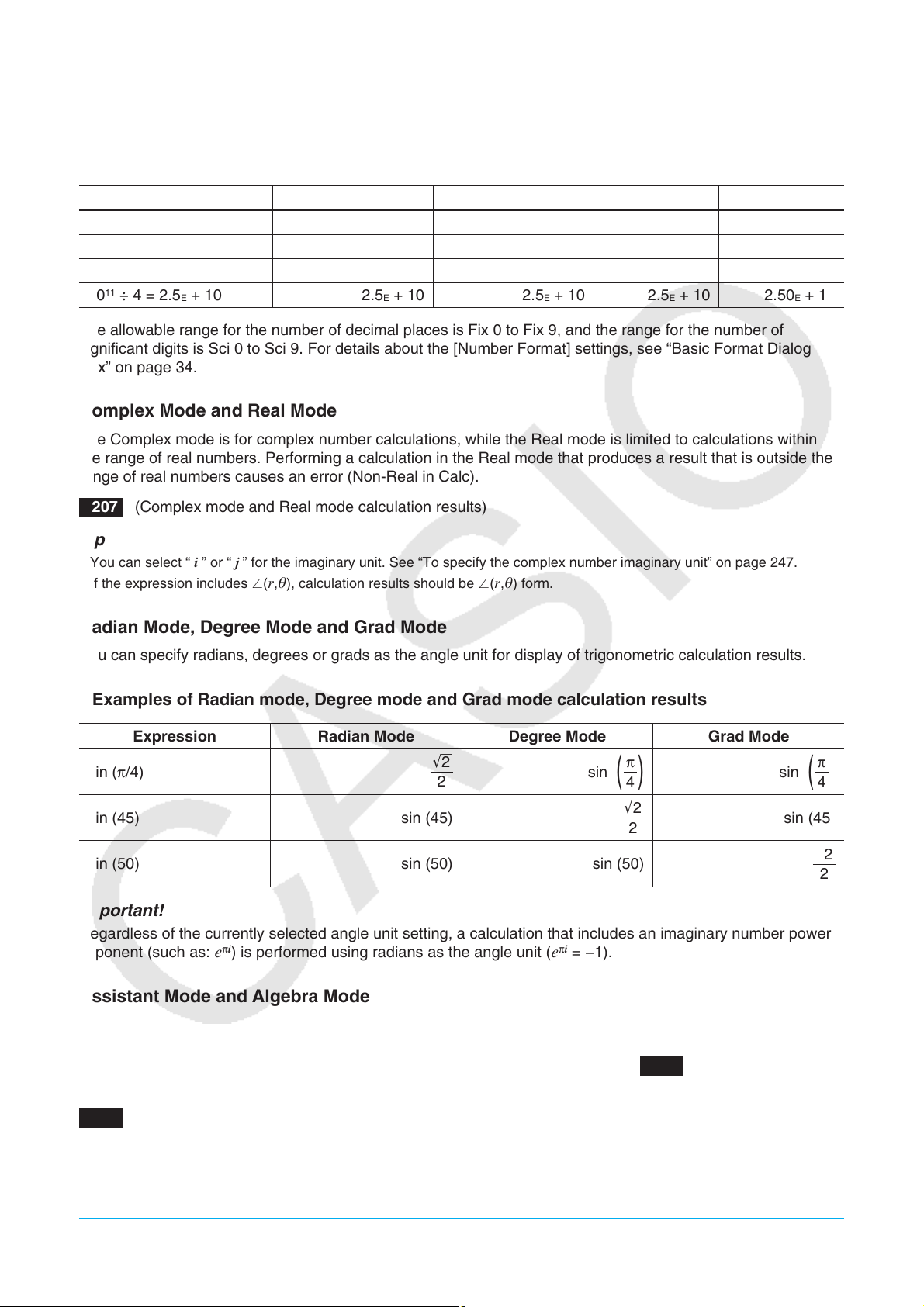
u Number of Decimal Places, Number of Significant Digits, Normal Display Settings
The [Number Format] settings on the Basic Format dialog box specify the number of decimal places, the
number of significant digits, and the normal display setting for Main application Decimal mode calculation
results. The following shows how calculation results appear under each setting.
Expression Normal 1 Normal 2 Fix 3 Sci 3
50 ÷ 4 = 12.5 12.5 12.5 12.500 1.25
100 ÷ 6 = 16.6666666... 16.66666667 16.66666667 16.667 1.67
1 ÷ 600 = 0.00166666... 1.666666667
11
÷ 4 = 2.5E + 10 2.5E + 10 2.5E + 10 2.5E + 10 2.50E + 10
10
The allowable range for the number of decimal places is Fix 0 to Fix 9, and the range for the number of
significant digits is Sci 0 to Sci 9. For details about the [Number Format] settings, see “Basic Format Dialog
Box” on page 34.
–3 0.00166666666 0.002 1.67E – 3
E
+ 1
E
+ 1
E
Complex Mode and Real Mode
The Complex mode is for complex number calculations, while the Real mode is limited to calculations within
the range of real numbers. Performing a calculation in the Real mode that produces a result that is outside the
range of real numbers causes an error (Non-Real in Calc).
0207 (Complex mode and Real mode calculation results)
Tip
• You can select “ i ” or “ j ” for the imaginary unit. See “To specify the complex number imaginary unit” on page 247.
• If the expression includes ⬔(
r , ), calculation results should be ⬔( r , ) form.
Radian Mode, Degree Mode and Grad Mode
You can specify radians, degrees or grads as the angle unit for display of trigonometric calculation results.
u Examples of Radian mode, Degree mode and Grad mode calculation results
Expression Radian Mode Degree Mode Grad Mode
sin (π/4)
sin (45) sin (45) sin (45)
sin (50) sin (50) sin (50)
'
sin
π
( )
4
'
sin
π
( )
4
'
Important!
Regardless of the currently selected angle unit setting, a calculation that includes an imaginary number power
exponent (such as: e
π
i
) is performed using radians as the angle unit (e
π
i
= −1).
Assistant Mode and Algebra Mode
The Algebra mode automatically simplifies mathematical expressions produced by calculations. No
simplification is performed in the Assistant mode. In the Assistant mode, you can view intermediate results as
well, which allows you to see the steps that lead to a particular result as shown in 0208 (see the “expand”
example).
0208 (Assistant mode and Algebra mode calculation results)
Important!
The Assistant mode is available in the Main application and eActivity application only.
Chapter 2: Main Application 45
Page 46

2-2 Using the Calculation History
The Main application work area calculation history can contain up to 30 expression/result pairs. You can look
up a previous calculation, edit, and then re-calculate it, if you want.
• Use the scroll bar or scroll buttons to scroll the work area window up and down. This brings current calculation
history contents into view.
• You can edit a calculation expression in the calculation history and then re-calculate the resulting expression.
Pressing E re-calculates the expression where the cursor is currently located, and also re-calculates all of
the expressions below the current cursor location.
0209 To change the expression “ans × 2” to “ans × 3” in the example, and then re-calculate
Tip
• To re-calculate only a single specific line, tap 7. Tapping 7 re-calculates the calculation where the cursor is currently
located only. It does not affect anything in calculation history that comes before or after the line.
• To re-calculate all of the expressions in the calculation history, locate the cursor in the top line, and then press E.
u To delete part of the calculation history contents
1. Move the cursor to the expression line or result line of the two-line unit you want to delete.
2. Tap [Edit] and then [Delete].
Important!
Even if the result of the deleted two-line unit has an effect on subsequent calculations, the affected calculations
are not updated automatically following the deletion. When you want to update everything in the calculation
history following the deleted unit, move the cursor to a line that is above the one you deleted and then press
E.
u To clear all calculation history contents
Tap [Edit] and then [Clear All]. In response to the confirmation message that appears, tap [OK].
2-3 Function Calculations
This section explains how to perform function calculations in the Main application work area.
• You do not need to input the closing parenthesis that comes immediately before an E key operation. All of
the calculation examples in this section omit the closing parentheses before E.
• The following example calculations are all performed using the Decimal mode. Using the Standard mode
causes results to be displayed as fractions.
Angle Conversion (°, r)
The first two examples use “Degree” (indicated by “Deg” in the status bar) as the angle unit setting. The final
example uses “Radian” (indicated by “Rad” in the status bar) as the angle unit setting. Note that using the
wrong angle unit setting will make it impossible to produce correct calculation results.
u To change the angle unit setting
1. On the O menu, tap [Basic Format].
2. Tap the [Angle] down arrow button, and then select [Radian], [Degree] or [Grad].
• You can also change the angle unit setting by tapping the current setting (Rad, Deg, or Gra) on the status
bar. Each tap will cycle through the available settings.
Chapter 2: Main Application 46
Page 47
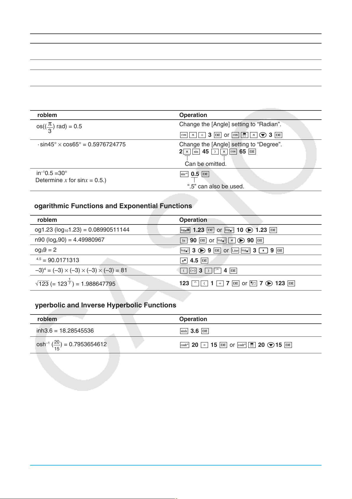
Problem Operation
Convert 4.25 radians to degrees.
4.25 Rw
= 243.5070629
47.3° + 82.5rad = 4774.20181°
How many radians is 243.5070629°?
= 4.249999999
47.3 + 82.5 Rw
Change the [Angle] setting to “Radian”, and then
input 243.5070629 *w.
Trigonometric and Inverse Trigonometric Functions
Problem Operation
π
cos((
2
) rad) = 0.5
3
·
sin45° × cos65° = 0.5976724775
Change the [Angle] setting to “Radian”.
c7/ 3 w or cN7c 3 w
Change the [Angle] setting to “Degree”.
2*s 45 )*c 65 w
Can be omitted.
–1
0.5 =30°
sin
S 0.5 w
(Determine x for sin x = 0.5.)
“.5” can also be used.
Logarithmic Functions and Exponential Functions
Problem Operation
log1.23 (log
ln90 (log
9 = 2
log
3
4.5
e
= 90.0171313
4
(–3)
= (–3) × (–3) × (–3) × (–3) = 81
7
123 (= 123
1.23) = 0.08990511144
10
90) = 4.49980967
e
1
7
) = 1.988647795
" 1.23 w or V 10 e 1.23 w
I 90 w or V`e 90 w
V 3 e 9 w or LV 3 , 9 w
Q 4.5 w
(- 3 ){ 4 w
123 {( 1 / 7 w or % 7 e 123 w
Hyperbolic and Inverse Hyperbolic Functions
Problem Operation
sinh3.6 = 18.28545536
–1
(
cosh
) = 0.7953654612
1 3.6 w
@ 20 / 15 w or @N 20 c15 w
Chapter 2: Main Application 47
Page 48

Other Functions (%, ', x2, x –1, x!, abs, ⬔, signum, int, frac, intg, fRound, sRound)
Problem Operation
What is 12% of 1500? (180)
What percent of 880 is 660? (75%)
What value is 15% greater than 2500? (2875)
What value is 25% less than 3500? (2625)
'2 + '5 = 3.65028154
(3 + i ) = 1.755317302 + 0.2848487846 i Change to the Complex mode (“Cplx” indicated on
2
= (–3) × (–3) = 9
(–3)
2
= –(3 × 3) = –9
–3
1
= 12
1
1
–
4
3
8! (= 1 × 2 × 3 × … × 8) = 40320
What is the absolute value of the common
3
logarithm of
3
⎜log (
)⎟ = 0.1249387366
4
?
4
8⬔40° × 5⬔35°
⬔(8,40) × ⬔(5,35) = ⬔(40,75)
What is the sign of –3.4567? (–1)
(signum returns –1 for a negative value, 1 for a
positive value, “Undefined” for 0, and
imaginary number.)
$
²$´
for an
What is the integer part of –3.4567? (–3)
What is the decimal part of –3.4567? (–0.4567)
What is the greatest integer less than or equal to
–3.4567? (–4)
What is –3.4567 rounded to two decimal places?
(–3.46)
What is –34567 rounded to four significant digits?
(–34570)
* To round to 10 digits, specify “0” for the second argument.
1500 * 12 &w
660 / 880 &w
2500 *( 1 + 15 &
3500 *( 1 - 25 &
5 2 e+5 5 w
the status bar).
5 3 +0w
(- 3 )xw
- 3 xw
( 3 X- 4 X)Xw
or
N 1 cN 1 c 3 e-N 1 c 4 w
8 !w
4V 10 eN 3 c 4 w
or L4V 3 / 4 w
Change to the Degree mode (“Deg” indicated on the
status bar).
~ 8 , 40 )*~ 5 , 35 )w
[signum] - 3.4567 w
:- 3.4567 w
[frac] - 3.4567 w
[intg] - 3.4567 w
[fRound] - 3.4567 , 2 w
[sRound] - 34567 , 4 w*
Random Number Generator (rand, randList, randNorm, randBin, RandSeed)
The ClassPad random number generator can generate truly random numbers (non-sequential random
numbers) and random numbers that follow a particular pattern (sequential random numbers).
u To switch between non-sequential and sequential random number generation
1. Use the “RandSeed” command to configure random number generation settings. See “RandSeed
Command” on page 50.
2. Use the “rand”, “randList”, “randNorm”, or “randBin” function to generate the random numbers.
Chapter 2: Main Application 48
Page 49

u “rand” Function
The “rand” function generates random numbers. If you do not specify an argument, “rand” generates 10-digit
decimal values 0 or greater and less than 1.
Specifying two integer values for the argument generates random numbers between them.
Problem Operation
Generate random numbers between 0 and 1.
Generate random integers between 1 and 6.
[rand] w
[rand] 1 , 6 w
u “randList” Function
Syntax: randList( n [, a, b])
Function:
• Omitting arguments “a” and “b” returns a list of
• Specifying arguments “a” and “b” returns a list of
of “a” through “b”.
Description:
• “
n ” must be a positive integer.
• The random numbers of each element are generated in accordance with “RandSeed” specifications, as with
the “rand” function.
n elements that contain decimal random values.
n elements that contain integer random values in the range
Problem Operation
Generate a list of three elements that contain
decimal random values.
Generate a list of five elements that contain random
values in the range of 1 through 6.
[randList] 3 w
[randList] 5 , 1 , 6 w
u “randNorm” Function
The “randNorm” function generates a 10-digit normal random number based on a specified mean and
standard deviation values.
Syntax: randNorm(
Function:
• Omitting a value for “
• Specifying a value for “
Description:
• “
n ” must be a positive integer, and “ ” must be greater than 0.
Problem Operation
Randomly produce a body length value obtained in
accordance with the normal distribution of a group
of infants less than one year old with a mean body
length of 68 cm and standard deviation of 8.
Randomly produce the body lengths of five infants in
the above example, and display them in a list.
, [, n ])
n ” (or specifying 1 for “ n ”) returns the generated random number as-is.
n ” returns the specified number of random values in list format.
[randNorm] 8 , 68 w
[randNorm] 8 , 68 , 5 w
u “randBin” Function
The “randBin” function generates binomial random numbers based on values specified for the number of trials
n and probability P.
Syntax: randBin( n , P [, m ])
Chapter 2: Main Application 49
Page 50

Function:
• Omitting a value for “
• Specifying a value for “
m ” (or specifying 1 for “ m ”) returns the generated random number as-is.
m ” returns the specified number of random values in list format.
Description:
• “
n ” and “ m ” must be positive integers.
Problem Operation
Randomly produce the number of heads that can be
[randBin] 5 , 0.5 w
expected in accordance with binomial distribution for
five coin tosses where the probability of heads is 0.5.
Perform the same coin toss sequence described
[randBin] 5 , 0.5 , 3 w
above three times and display the results in a list.
u “RandSeed” Command
• You can specify an integer from 0 to 9 for the argument of this command. 0 specifies non-sequential random
number generation. An integer from 1 to 9 uses the specified value as a seed for specification of sequential
random numbers. The initial default argument for this command is 0.
• The numbers generated by the ClassPad immediately after you specify sequential random number generation
always follow the same random pattern.
Problem Operation
Generate sequential random numbers using 3 as the
seed value.
Generate the first value.
Generate the second value.
Generate the third value.
[RandSeed] 3 w
[rand] w
[rand] w
[rand] w
Tip
• Random values generated by these commands are pseudo random values.
• The arguments a and b of “rand(a,b)” and “randList(n,a,b)” must be integers, subject to the following conditions.
a < b
⎟ a⎟ , ⎟ b⎟ < 1
10 b – a < 1E10
E
Integer Functions
These functions take integers only as their arguments and return integers.
u “iGcd” Function
Syntax: iGcd(Exp-1, Exp-2[, Exp-3…Exp-10)]
(Exp-1 through Exp-10 all are integers.)
iGcd(List-1, List-2[, List-3…List-10)]
(All elements of List-1 through List-10 are integers.)
Function:
• The first syntax above returns the greatest common divisor for two to ten integers.
• The second syntax returns, in list format, the greatest common divisor (GCD) for each of the elements in two
to ten lists. When the arguments are {
and c , and for b and d .
Description:
• All of the lists must have the same number of elements.
• When using the “iGcd(List-1, List-2[, List-3…List-10)]” syntax, one (and only one) expression (Exp) can be
include as an argument in place of a list.
a , b }, { c , d }, for example, a list will be returned showing the GCD for a
Chapter 2: Main Application 50
Page 51

Problem Operation
Determine the greatest common divisors of {4, 3},
{12, 6}, and {36, 9}.
[iGcd] { 4 , 3 },{ 12 , 6 },{ 36
, 9 })w
u “iLcm” Function
Syntax: iLcm(Exp-1, Exp-2[, Exp-3…Exp-10)]
(Exp-1 through Exp-10 all are integers.)
iLcm(List-1, List-2[, List-3…List-10)]
(All elements of List-1 through List-10 are integers.)
Function:
• The first syntax above returns the least common multiple for two to ten integers.
• The second syntax returns, in list format, the least common multiple (LCM) for each of the elements in two to
ten lists. When the arguments are {
and for b and d .
Description:
• All of the lists must have the same number of elements.
• When using the “iLcm(List-1, List-2[, List-3…List-10)]” syntax, one (and only one) expression (Exp) can be
include as an argument in place of a list.
Problem Operation
Determine the least common multiples of {4, 3},
{12, 6}, and {36, 9}.
a , b }, { c , d }, for example, a list will be returned showing the LCM for a and c ,
[iLcm] { 4 , 3 },{ 12 , 6 },{ 36
, 9 })w
u “iMod” Function
Syntax: iMod(Exp-1/List-1, Exp-2/List-2[)]
Function:
• This function divides one or more integers by one or more other integers and returns the remainder(s).
Description:
• Exp-1 and Exp-2, and all of the elements of List-1 and List-2 must be integers.
• You can use Exp for one argument and List for the other argument (Exp, List or List, Exp) if you want.
• If both arguments are lists, both lists must have the same number of elements.
Problem Operation
Divide 21 by 6 and 7, and determine the remainder
[iMod] 21 ,{ 6 , 7 })w
of both operations. (iMod(21, {6, 7})
Permutation (nPr) and Combination (nCr)
u Total Number of Permutations
u Total Number of Combinations
3
&
Problem Operation
To determine the number of permutations and combinations
possible when selecting four people from a group of 10
²²²²²
²
²²²²²²²
²
10P4
10C4
= 5040
= 210
} 10 , 4 w
{ 10 , 4 w
Chapter 2: Main Application 51
Page 52

Condition Judgment (judge, piecewise)
u “judge” Function
The “judge” function returns TRUE when an expression is true, and FALSE when it is false.
Problem Operation
Is the following expression true or false?
1 = 1 TRUE
Is the following expression true or false?
1 < 0 FALSE
[judge] 1 = 1 w
[judge] 1 < 0 w
u “piecewise” Function
The “piecewise” function returns one value when an expression is true, and another value when the expression
is false.
The syntax of the “piecewise” function is shown below.
piecewise(<condition expression>, <return value when true>, <return value when false or indeterminate> [ ) ]
or
piecewise(<condition expression>, <return value when true>, <return value when false>, <return value when
indeterminate> [ ) ]
Use the soft keyboard (1) to input “piecewise” function according to the syntax shown below.
<return value when true>, <condition expression>
<return value when false or indeterminate>
or
<return value when condition 1 is true>, <condition 1 expression>
<return value when condition 2 is true>, <condition 2 expression>
Problem Operation
For the expression 0 t
when x is 0 or less, and 2 when x is greater than 0
or undefined.
For the expression 1 t
when x is 1 or less, and 2 when x is greater than 1.
x ( x = variable), return 1
x ( x = variable), return 1
[piecewise] 0 :X, 1 , 2 w
or
1 1 c 2 ef 0 :X w
1 1 c 2 ef 1 :X c 1 <Xw
Angle Symbol (∠)
Use this symbol to specify the coordinate format required by an angle in a vector.
You can use this symbol for a vector only.
Problem Operation
Convert the polar coordinates
rectangular coordinates. [1, 1]
r = '2 ,
θ
= π /4 to
Change the [Angle] setting to “Radian”.
[toRect] [5 2 e,~7/ 4 )]w
Derivative Symbol (’)
A single derivative symbol indicates the first derivative of an equation in the format: <variable name>’.
Problem Operation
Solve the differential equation
{ y = 0.5 · x 2 + const (1)}
y ’ = x .
+Y'=X,X,Yw
Important!
The “dSolve” function can solve differential equations up to three degrees, so a maximum of three derivative
symbols ( y ’’’) can be used. Executing a “dSolve” calculation that has more than three derivative symbols will
result in an Invalid Syntax error.
Chapter 2: Main Application 52
Page 53

Primality Test (isPrime)
The “isPrime” function determines whether the number provided as the argument is prime (returns TRUE) or
not (returns FALSE). The syntax of the “isPrime” function is shown below.
isPrime(Exp/List[ ) ]
• Exp or all of the elements of List must be integers.
Problem Operation
Determine whether the numbers 51 and 17 are
[isPrime] { 51 , 17 })w
prime.
(isPrime({51, 17})
Equal Symbols and Unequal Symbols (=, ≠, <, >, s, t)
You can use these symbols to perform a number of different basic calculations.
Problem Operation
To add 3 to both sides of
x = 3. x + 3 = 6
(X= 3 )+ 3 w
Subtract 2 from both sides of
y s 5. y – 2 s 3 (Y; 5 )- 2 w
Tip
• In the “Syntax” explanations of each command under “2-7 Using the Action Menu”, the following operators are indicated
as “Eq/Ineq”: =, ≠, <, >, s, t. Whether or not the “Eq/Ineq” operators include the “≠” operator is specified for each
command by a separate note.
• An expression that contains multiple equation or inequality operators cannot be input as a single expression. For output
expressions, an expression can be output with multiple operators only in the case of inequality operators that are facing in
the same direction (example: –1 <
x < 1).
Example: solve( x 2 – 1 < 0, x ) w {–1 < x < 1}
“with” Operator ( | )
The “with” ( I ) operator temporarily assigns a value to a variable. You can use the “with” operator in the
following cases.
• To assign the value specified on the right side of | to the variable on the left side of |
• To limit or restrict the range of a variable on the left side of | in accordance with conditions provided on the
right side of |
The following is the syntax for the “with” ( I ) operator.
Exp/Eq/Ineq/List/Mat|Eq/Ineq/List/(and operator)
You can put plural conditions in a list or connected with the “and” operator on the right side.
“” can be used on the left side or the right side of |.
Problem Operation
2
x
Evaluate
x
For
+ x + 1 when x = 3. 13
2
– 1 = 0, determine the value of x when x > 0.
X{ 2 +X+ 1 UX= 3 w
.X{ 2 - 1 = 0 ,X)UX> 0 w
{ x = 1}
Determine the value of abs (
x ) when x > 0. x
4XeUX> 0 w
Chapter 2: Main Application 53
Page 54

Solutions Supported by ClassPad (TRUE, FALSE, Undefined, No Solution, ∞, const, constn)
Solution Description Example
TRUE Output when a solution is true.
FALSE Output when a solution is false.
Undefined Output when a solution is undefined.
No Solution Output when there is no solution.
∞
const Constant displayed as const(1) when any value that is a
constn Constant displayed as constn(1) when the solution
Infinity
constant is included in the solution. In the case of multiple
constants, they are indicated as const(1), const(2), and
so on.
includes any integer value that is a constant. In the case
of multiple constants, they are indicated as constn(1),
constn(2), and so on.
judge (1 = 1) w
judge (1 < 0) w
1/0 w
solve (abs (
lim (1/
dSolve (
{ y = 0.5· x 2 + const (1)}
Change the [Angle] setting to
“Degree”.
solve (sin (
{ x = 180·constn (1)}
x ) = –1, x ) w
2
x
, x , 0) w
y = x , x , y ) w
x ) = 0, x ) w
Dirac Delta Function
“delta” is the Dirac Delta function. The delta function evaluates numerically as shown below.
b
Non-numeric expressions passed to the delta function are left unevaluated. The integral of a linear delta
function is a Heaviside function.
^
b
Syntax: delta(
0210 (Calculation example screenshot)
x )
x : variable or number
n th-Delta Function
The n th-delta function is the n th differential of the delta function.
Syntax: delta( x , n )
x : variable or number
n : number of differentials
0211 (Calculation example screenshot)
Heaviside Unit Step Function
“heaviside” is the command for the Heaviside function, which evaluates only to numeric expressions as shown
below.
H
Any non-numeric expression passed to the Heaviside function will not be evaluated, and any numeric
expression containing complex numbers will return undefined. The derivative of the Heaviside function is the
Delta function.
!
Syntax: heaviside(
x : variable or number
0212 (Calculation example screenshot)
x )
Chapter 2: Main Application 54
Page 55

Gamma Function
t
The Gamma function is called “gamma” on the ClassPad.
+∞
x–1
–t
t
e
Γ(x) =
For an integer n the gamma is evaluated as shown below.
∫
0
d
²
K
^
The gamma is defined for all real numbers excluding zero and negative integers. It is also defined for all
complex numbers where either the real or imaginary part of the complex number is not an integer.
Gamma of a symbolic expression returns unevaluated.
Syntax: gamma(
x : variable or number
0213 (Calculation and graph example screenshots)
x )
!
s
2-4 List Calculations
This section explains how to input list data, and how to perform basic list calculations.
Inputting List Data in the Work Area
0214 To input the list {1, 2, 3} and assign it to LIST variable “lista” in the Main application work area
LIST Variable Element Operations
You can recall the value of any element of a LIST variable. You can also assign a value to any element in a list.
0215 To recall the second element of the “lista” list variable of example 0214
0216
To assign 5 to the second element of “lista”
Using a List in a Calculation
You can perform arithmetic operations between two lists, between a list and a numeric value, or between a list
and an expression, equation, or inequality.
Important!
• When you perform an arithmetic operation between two lists, both of the lists need to have the same number
of cells. An error will occur if they do not.
• An error will also occur whenever an operation between any two cells of the two lists results in an error.
0217 Perform the operation list3 × {6, 0, 4} when list3 contains {41, 65, 22}
Using a List to Assign Different Values to Multiple Variables
Use the procedure in this section when you want to use a list to assign various different values to multiple variables.
Syntax: List with Numbers S List with Variables
0218 Assign the values 10, 20, and 30, to variables x, y, and z respectively
Chapter 2: Main Application 55
Page 56
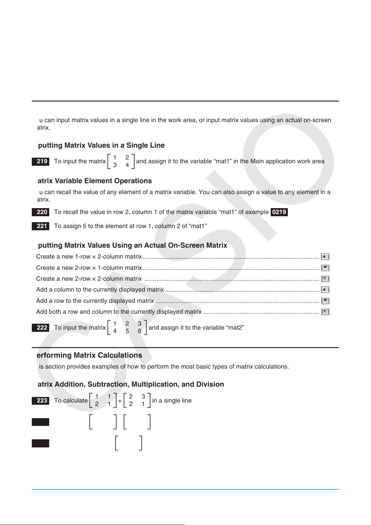
2-5 Matrix and Vector Calculations
This section explains how to create matrices, and how to perform basic matrix calculations.
Tip: Since a vector can be viewed as 1-row by n -column matrix or n -row by 1-column matrix, this section does not include
explanations specifically about vectors. For more information about vector-specific calculations, see the explanations
about the applicable [Action] menu items in “2-7 Using the Action Menu”.
Inputting Matrix Data
You can input matrix values in a single line in the work area, or input matrix values using an actual on-screen
matrix.
Inputting Matrix Values in a Single Line
0219 To input the matrix
1 2
3 4
and assign it to the variable “mat1” in the Main application work area
Matrix Variable Element Operations
You can recall the value of any element of a matrix variable. You can also assign a value to any element in a
matrix.
0220 To recall the value in row 2, column 1 of the matrix variable “mat1” of example 0219
0221
To assign 5 to the element at row 1, column 2 of “mat1”
Inputting Matrix Values Using an Actual On-Screen Matrix
• Create a new 1-row × 2-column matrix ...................................................................................................... 6
• Create a new 2-row × 1-column matrix ...................................................................................................... 7
• Create a new 2-row × 2-column matrix ..................................................................................................... 8
• Add a column to the currently displayed matrix ......................................................................................... 6
• Add a row to the currently displayed matrix ............................................................................................... 7
• Add both a row and column to the currently displayed matrix ................................................................... 8
0222 To input the matrix
1 2 3
4 5 6
and assign it to the variable “mat2”
Performing Matrix Calculations
This section provides examples of how to perform the most basic types of matrix calculations.
Matrix Addition, Subtraction, Multiplication, and Division
0223 To calculate
0224 To calculate
0225 To multiply the matrix
1 1
2 1
1 1
2 1
+
×
1 2
3 4
2 3
2 1
2 3
2 1
in a single line
using an actual on-screen matrix
by 5
Chapter 2: Main Application 56
Page 57

Raising a Matrix to a Specific Power
Example: To raise
0226 Input in a single line
0227 Input using an actual on-screen matrix
1 2
3 4
to the power of 3
Tip: You can raise only a square matrix to a specific power. An error occurs when you try to raise a non-square matrix to a
specific power.
Using a Matrix to Assign Different Values to Multiple Variables
Use the procedure in this section when you want to use a matrix to assign various different values to multiple
variables.
Syntax: Matrix with Numbers ⇒ Matrix with Variables
(The matrix can be one line with multiple columns, or multiple lines with one column.)
0228 Assign the values 10, 20, and 30, to variables x , y , and z respectively
2-6 Specifying a Number Base
While using the Main application, you can specify a default number base (binary, octal, decimal, hexadecimal).
You can also convert between number bases and perform bitwise operations using logical operators (not, and,
or, xor).
Note the following limitations, which all apply while a default number base (binary, octal, decimal, hexadecimal)
is specified in the Main application.
• You cannot use scientific functions, or [Action] or [Interactive] menu commands.
• Except for Ans (Answer Memory variable), you cannot use variables.
• You can input integers only. An error (Invalid Syntax) will occur if you try to input a non-integer value (like 1.5
or '2 ).
• If a calculation produces a non-integer result (with a decimal part), the ClassPad will cut off the decimal part
automatically. For example, the calculation 5 ÷ 2 while decimal is selected as the number base is 2.
• An error message is displayed if you try to enter a value that is invalid for the speicfied number base. The
following shows the numerals that can be used in each number system.
Binary: 0, 1 Octal: 0 to 7 Decimal: 0 to 9 Hexadecimal: 0 to 9, A, B, C, D, E, F
Binary, Octal, Decimal, and Hexadecimal Calculation Ranges
• The following are the display capacities and calculation ranges for each of the number bases.
Number Base Display Capacity Calculation Range (Positive ; Negative)
Binary 32 digits
Octal 11 digits
Decimal 10 digits
Hexadecimal 8 digits
x s 01111111111111111111111111111111 ;
0 s
10000000000000000000000000000000 s x s
11111111111111111111111111111111
x s 17777777777 ; 20000000000 s x s 37777777777
0 s
x s 2147483647 ; −2147483648 s x s −1
0 s
x s 7FFFFFFF ; 80000000 s x s FFFFFFFF
0 s
• Negative binary, octal, and hexadecimal values are produced using the two’s complement of the original
value.
Chapter 2: Main Application 57
Page 58

Selecting a Number Base
Specifying a default number base in the Main application will apply to the current line (expression/result pair),
and to all subsequent lines until you change the default number base setting.
u To select the number base for the line where the cursor is located
1. Tap the down arrow button next to the < button.
2. Tap the button that corresponds to the number base you want to use:
1 (binary), 2 (octal), 3 (decimal), 4 (hexadecimal).
• The currently selected number base is indicated in the status bar.
3. Execute the calculation.
Important!
• A line for which a number base is not specified is called a “normal calculation line”. To return a line to a
normal calculation line, tap < in step 2 of the above procedure.
• Calculation results produced by a line for which a number base is specified are followed by one of the suffixes
listed below, to indicate its number system.
Number System Binary Octal Decimal Hexadecimal
Suffix bodh
u To specify a number base for an input value
You can input the following suffixes to specify the number base of a value as you input it: [b] (binary), [o] (octal),
[d] (decimal), and [h] (hexadecimal). You can specify a number base for an input value only when a default
number base (besides normal) is selected
Arithmetic Operations
You can use the following operators when performing binary, octal, decimal and hexadecimal values: +, −, ×, ÷,
^. You can also use parenthetical expressions.
0229 To calculate 101112 + 11010
0230 To calculate (118 + 78)
0231 Perform the calculation 12310 + 10102 so it produces a hexadecimal result
2
2
Bitwise Operations
The logical operators (and, or, xor, not) can be used in calculations.
and ...Returns the result of a bitwise product.
or ...... Returns the result of a bitwise sum.
xor ....Returns the result of a bitwise exclusive logical sum.
not ....Returns the result of a complement (bitwise inversion).
0232 Calculation examples
Chapter 2: Main Application 58
Page 59

Using the baseConvert Function (Number System Transform)
The baseConvert function lets you convert a number in one base (number system) to its equivalent in another
base.
Important!
• The baseConvert function works for positive integers only.
• The baseConvert function cannot be used in a line for which a particular number base is specified. It can be
used in a normal calculation line only.
Syntax: baseConvert (Number, Current base, Expected base)
• Number must be a positive integer consisting of digits 0 to 9 and/or A to F.
• The current base and expected base can be any whole number from 2 to 16.
0233 Calculation examples
2-7 Using the Action Menu
The [Action] menu helps to make transformation and expansion functions, calculus functions, statistical
functions, and other frequently used mathematical menu operations easier to use. Simply select the function
you want, and then enter expressions or variables in accordance with the syntax of the function.
Tip
• Unless specifically indicated otherwise, all of the explanations in this section are performed using the following modes:
Algebra mode, Standard mode, Complex mode, Radian mode, Descending Order.
• You can use the [Interactive] menu to select most of the commands that are included on the [Action] menu. For details
about using the [Interactive] menu, see page 89.
Abbreviations and Punctuation Used in This Section
The following are the meanings of the abbreviations and punctuation used in the syntax descriptions in this section.
Exp: Expression (Value, Variable, etc.) List: List
Eq: Equation Mat: Matrix
Ineq: All types of inequalities (a>b, atb, a<b, asb, ab)
Ineqⴝ: Inequality ab only
[ ]: You can omit the item(s) inside the brackets.
{ }: Select one of the items inside the braces.
Some of the syntaxes in the following explanations indicate the following for parameters:
Exp/Eq/Ineq/List/Mat
These abbreviations mean that you can use any of the following as a parameter: expression, equation,
inequality, list, or matrix.
Chapter 2: Main Application 59
Page 60

Example Screenshots
The screenshots below show examples of how input and output expressions appear on the ClassPad display.
All of the screenshots in this section show the “complete expression” version.
When the input expression does not fit:
Displayed expression
When the output expression does not fit:
Displayed expression
Complete expression
Complete expression
Using the Transformation Submenu
The [Transformation] submenu contains commands for expression transformation, like “expand” and “factor”.
u approx [Action][Transformation][approx]
Function: Transforms an expression into a numerical approximation.
)
Syntax: approx (Exp/Eq/Ineq/List/Mat [
Example: To obtain the numerical value of '2
u simplify [Action][Transformation][simplify]
Function: Simplifies an expression.
Syntax: simplify (Exp/Eq/Ineq/List/Mat [ ) ]
]
Example: To simplify (15'3 + 26)^(1/3)
u expand [Action][Transformation][expand]
Function: Expands an expression.
)
Syntax: expand (Exp/Eq/Ineq/List/Mat [
expand (Exp,variable [ ) ]
• If you specify a variable, Exp is decomposed into partial fractions, with
respect to the variable.
Example: To expand (
x + 2)
2
]
u factor [Action][Transformation][factor][factor]
Function: Factors an expression.
Syntax: factor (Exp/Eq/Ineq/List/Mat [ ) ]
2
x
Example: To factor
4 x + 4
Chapter 2: Main Application 60
Page 61
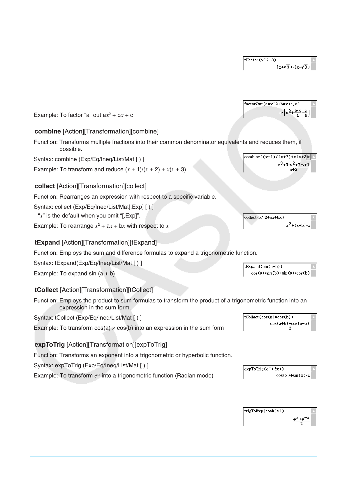
u rFactor [Action][Transformation][factor][rFactor]
Function: Factors an expression up to its roots, if any.
Syntax: rFactor (Exp/Eq/Ineq/List/Mat [ ) ]
2
x
Example: To factor
3
u factorOut [Action][Transformation][factor][factorOut]
Function: Factors out an expression with respect to a specified factor.
Syntax: factorOut (Exp/Eq/Ineq/List/Mat, Exp [ ) ]
2
x
Example: To factor “a” out a
+ b x + c
u combine [Action][Transformation][combine]
Function: Transforms multiple fractions into their common denominator equivalents and reduces them, if
possible.
Syntax: combine (Exp/Eq/Ineq/List/Mat [ ) ]
Example: To transform and reduce (
x + 1)/( x + 2) + x ( x + 3)
u collect [Action][Transformation][collect]
Function: Rearranges an expression with respect to a specific variable.
Syntax: collect (Exp/Eq/Ineq/List/Mat[,Exp] [ ) ]
• “
x ” is the default when you omit “[,Exp]”.
2
x
Example: To rearrange
+ a x + b x with respect to x
u tExpand [Action][Transformation][tExpand]
Function: Employs the sum and difference formulas to expand a trigonometric function.
Syntax: tExpand(Exp/Eq/Ineq/List/Mat [ ) ]
Example: To expand sin (a + b)
u tCollect [Action][Transformation][tCollect]
Function: Employs the product to sum formulas to transform the product of a trigonometric function into an
expression in the sum form.
Syntax: tCollect (Exp/Eq/Ineq/List/Mat [ ) ]
Example: To transform cos(a) × cos(b) into an expression in the sum form
u expToTrig [Action][Transformation][expToTrig]
Function: Transforms an exponent into a trigonometric or hyperbolic function.
Syntax: expToTrig (Exp/Eq/Ineq/List/Mat [ ) ]
ix
e
Example: To transform
into a trigonometric function (Radian mode)
u trigToExp [Action][Transformation][trigToExp]
Function: Transforms a trigonometric or hyperbolic function into exponential form.
Syntax: trigToExp (Exp/Eq/Ineq/List/Mat [ ) ]
Example: To transform cosh
x into exponential form
Chapter 2: Main Application 61
Page 62

u toFrac [Action][Transformation][Fraction][toFrac]
Function: Transforms a decimal value into its equivalent fraction value.
Syntax: toFrac (Exp/Eq/Ineq/List/Mat [ ) ]
Example: To transform 5.28 into its equivalent fraction value
u propFrac [Action][Transformation][Fraction][propFrac]
Function: Transforms a decimal value into its equivalent proper fraction value.
Syntax: propFrac (Exp/Eq/Ineq/List/Mat [ ) ]
Example: To transform 1.2 into its equivalent proper fraction value
u dms [Action][Transformation][DMS][dms]
Function: Transforms a DMS format value into its equivalent degrees-only
value.
Syntax: dms (Exp/List-1 [,Exp/List-2][,Exp/List-3] [ ) ]
Example: To transform 3° 5’ 6” into its equivalent degrees-only value
• Zero is the default when you omit [,Exp/List-2] or [,Exp/List-3][ ) ].
Tip: You can input 3° 5’ 6” using the / key on the soft keyboard.
/e 3 e 5 e 6 E
u toDMS [Action][Transformation][DMS][toDMS]
Function: Transforms a degrees-only value into its equivalent DMS format value.
Syntax: toDMS (Exp/List [ ) ]
Example: To transform 3.085 degrees into its equivalent DMS format value
Using the Advanced Submenu
u solve [Action][Advanced][solve]
For information about solve, see page 79.
u dSolve [Action][Advanced][dSolve]
For information about dSolve, see page 80.
u taylor [Action][Advanced][taylor]
Function: Finds a Taylor polynomial for an expression with respect to a specific variable.
)
Syntax: taylor (Exp/List, variable, order [,center point] [
Example: To find a 5th order Taylor polynomial for sin(x) with respect to x = 0
(in the Radian mode)
• Zero is the default when you omit “[,center point]”.
]
u laplace [Action][Advanced][laplace], invLaplace [Action][Advanced][invLaplace]
Function: “laplace” is the command for the Laplace transform, and
“invLaplace” is the command for the inverse of Laplace transform.
Chapter 2: Main Application 62
∞
∫
0
()
–
L[ ()] ()=
Page 63

Syntax:
∞
–∞
()
ω
(ω) =
⏐
⏐
(2
π)
1–
∞
–∞
(ω)
–ω
ω
() =
⏐
⏐
(2
π)
1+
laplace(
f ( t): expression ;
f ( t), t, s)
t: variable with respect to which the expression is
transformed ;
s: parameter of the transform
invLaplace(
L(s), s, t)
L(s): expression ;
s: variable with respect to which the expression is
transformed ;
t: parameter of the transform
ClassPad supports transform of the following functions.
x), cos(x), sinh(x), cosh(x), x
sin(
n
, 'x, ex, heaviside(x), delta(x), delta(x, n)
ClassPad does not support transform of the following functions.
tan(
x), sin
– 1
(x), cos
– 1
(x), tan
– 1
(x), tanh(x), sinh
– 1
(x), cosh
– 1
(x), tanh
– 1
(x), log(x), ln(x), 1/x, abs(x), gamma(x)
Laplace Transform of a Differential Equation
The laplace command can be used to solve ordinary differential equations. ClassPad does not support System
of Differential Equations for laplace.
Syntax: laplace(diff eq,
diff eq: differential equation to solve ; x : independent variable in the diff eq ;
y : dependent variable in the diff eq ; t : parameter of the transform
Example: To solve a differential equation
Laplace transform
Lp means F ( s ) = L [ f ( t )] in the result of transform for a differential equation.
x , y , t )
x ’ + 2 x = e
t
−
where x (0) = 3 using the
u fourier [Action][Advanced][fourier], invFourier [Action][Advanced][invFourier]
Function: “fourier” is the command for the Fourier Transform, and “invFourier” is the command for the inverse
Fourier Transform.
Syntax: fourier( f ( x), x, w, n) invFourier( f ( w), w, x, n)
x : variable with respect to which the expression is transformed with ; w : parameter of the transform ;
n : 0 to 4, indicating Fourier parameter to use (optional)
ClassPad supports transform of the following functions.
t), cos(t), log(t), ln(t), abs(t), signum(t), heaviside(t), delta(t), delta(t,n), e
sin(
ClassPad does not support transform of the following functions.
tan(t), sin
– 1
(t), cos
– 1
(t), tan
– 1
(t), sinh(t), cosh(t), tanh(t), sinh
– 1
(t), cosh
The Fourier Transform pairs are defined using two arbitrary constants a, b.
∫
The values of a and b depend on the scientific discipline, which can be specified by the value of n (optional
fourth parameter of fourier and invFourier) as shown below.
– 1
(t), tanh
∫
ti
– 1
(t), gamma(t), 't , e
t
Chapter 2: Main Application 63
Page 64

Transform Definition
Modern Physics 0 0 1
Pure Math 1 1 –1
Probability 2 1 1
Classical Physics 3 –1 1
Signal Processing 4 0
Tip: The Advanced Format dialog box can be used to configure settings related to the Fourier Transform, such a Fourier
Transform definition, etc. For details, see “Advanced Format Dialog Box” on page 38.
u FFT [Action][Advanced][FFT], IFFT [Action][Advanced][IFFT]
Function: “FFT” is the command for the fast Fourier Transform, and “IFFT” is the command for the inverse fast
Fourier Transform. 2n data values are needed to perform FFT and IFFT. On the ClassPad, FFT and
IFFT are calculated numerically.
n (optional) a b
–2*π
Syntax: FFT(list) or FFT(list,
• Data size must be 2
• The value for
0 (Signal Processing), 1 (Pure Math), 2 (Data Analysis).
The Fourier Transform is defined as the following:
∞
() =
Some authors (especially physicists) prefer to write the transform in terms of angular frequency ω ≡ 2π
instead of the oscillation frequency .
However, this destroys the symmetry, resulting in the transform pair shown below.
∫
–∞
(ω) = [()] =
To restore the symmetry of the transforms, the convention shown below is sometimes used.
() = [ ()] =
In general, the Fourier transform pair may be defined using two arbitrary constants a and b as shown below.
(ω) =
m ) IFFT(list) or IFFT(list, m )
n
for n = 1, 2, 3, ...
m is optional. It can be from 0 to 2, indicating the FFT parameter to use:
()
⏐
(2
2π
2
⏐
π)
1
1–
∫
π
–∞
∞
∫
∫
()
∞
–∞
∞
–∞
–ω
()
()
–
ω
∞
() =
∫
–∞
() = –1[(ω)] =
() = –1[()] =
() =
()
⏐
(2
⏐
π)
–2π
1+
2
1
∫
1
2
π
∞
–∞
∫
π
∞
∫
–∞
(ω)
∞
(ω)
–∞
()
–ω
ω
ω
ω
Unfortunately, a number of conventions are in widespread use for a and b . For example, (0, 1) is used in
modern physics, (1, –1) is used in pure mathematics and systems engineering, (1, 1) is used in probability
theory for the computation of the characteristic function, (–1, 1) is used in classical physics, and (0, –2π) is
used in signal processing.
Tip: The Advanced Format dialog box can be used to configure Fast Fourier Transform settings. For details, see
“Advanced Format Dialog Box” on page 38.
Chapter 2: Main Application 64
Page 65

Using the Calculation Submenu
The [Calculation] submenu contains calculus related commands, such as “diff” (differentiation) and “ ”
(integration).
u diff [Action][Calculation][diff]
Function: Differentiates an expression with respect to a specific variable.
Syntax: diff(Exp/List[,variable] [ ) ]
diff(Exp/List,variable,order[,a] [ ) ]
• “a” is the point for which you want to determine the derivative.
• “order” = 1 when you use the following syntax: diff(Exp/List[,variable][ ) ]. The default variable is “
“variable” is omitted.
6
x
Example: To differentiate
with respect to x
u impDiff [Action][Calculation][impDiff]
Function: Differentiates an equation or expression in implicit form with respect
to a specific variable.
Syntax: impDiff(Eq/Exp/List, independent variable, dependent variable)
x ” when
Example: To find
y ’ using implicit differentiation
Important!
The derivative symbol (’) cannot be used in the argument of “impDiff(”. Trying to use a derivative symbol
would result in a Wrong Argument Type error.
u∫ [Action][Calculation][ ]
Function: Integrates an expression with respect to a specific variable.
Syntax:
(Exp/List[,variable] [ ) ]
(Exp/List, variable, lower limit, upper limit [,tol ] [ ) ]
• “
x” is the default when you omit [,variable].
• “
tol” represents the allowable error range.
• This command returns an approximate value when a range is specified for “
• This command returns the true value of a definite interval when nothing is specified for “
cannot be obtained, however, this command returns an
approximate value along with tol =1E – 5.
Example: To integrate x with respect to x
tol ”.
tol ”. If the true value
u lim [Action][Calculation][lim]
Function: Determines the limit of an expression.
)
Syntax: lim (Exp/List, variable, point [,direction] [
−
x
e
Example: To determine the limit of
• This function returns the limit from the left when “direction” < 0, the limit from the right when “direction” > 0,
and the limit from both sides (left and right) when “direction” = 0 or when the direction is omitted.
as x approaches ∞
]
uΣ [Action][Calculation][Σ]
Function: Evaluates an expression at discrete variable values within a range, and then calculates a sum.
Syntax: Σ(Exp/List, variable, lower value, upper value [ ) ]
2
x
Example: To calculate the sum of
through x =10
as the value of x changes from x = 1
Chapter 2: Main Application 65
Page 66

uΠ [Action][Calculation][Π]
Function: Evaluates an expression at discrete variable values within a range, and then calculates a product.
Syntax: Π(Exp/List, variable, lower value, upper value [ ) ]
2
x
Example: To calculate the product of
as the value of x changes from x = 1
through x = 5
u rangeAppoint [Action][Calculation][rangeAppoint]
Function: Finds an expression or value that satisfies a condition in a specified range.
Syntax: rangeAppoint (Exp/Eq/List, start value, end value [ ) ]
• When using an equation (Eq) for the first argument, input the equation using the syntax Var = Exp.
Evaluation will not be possible if any other syntax is used.
Example: To find the expression(s) in the list {
x = π, x = 2π,
x = 3π} that belong(s) to the closed range 0 s x s 5
u mod [Action][Calculation][mod]
Function: Returns the remainder when one expression is divided by another expression.
Syntax: mod ({Exp/List} -1, {Exp/List} -2 [ ) ]
Example: To determine the remainder when 26 is divided by 3 (26mod3)
u tanLine [Action][Calculation][line][tanLine]
Function: Returns the right side of the equation for the tangent line ( y = ‘expression’) to the curve at the
specified point.
Syntax: tanLine (Exp/List, variable, variable value at point of tangency [ ) ]
3
y = x
Example: To determine the function of the line tangent to
at x = 2
u normal [Action][Calculation][line][normal]
Function: Returns the right side of the equation for the line normal ( y = ‘expression’) to the curve at the
specified point.
Syntax: normal (Exp/List, variable, variable value at point of normal [ ) ]
3
y = x
Example: To determine the function of the line normal to
at x = 2
u arcLen [Action][Calculation][line][arcLen]
Function: Returns the arc length of an expression from a start value to an end value with respect to a
specified variable.
Syntax: arcLen (Exp/List, variable, start value, end value [ ) ]
3
2
y = x
Example: To determine the arc length for
from x = 0 to x = 4
u fMin [Action][Calculation][fMin/fMax][fMin], fMax [Action][Calculation][fMin/fMax][fMax]
Function: Returns the minimum (fMin) / the maximum (fMax) point in a specific range of a function.
Syntax: fMin(Exp[,variable] [ ) ]
fMin(Exp, variable, start value, end value[,
fMax(Exp[,variable] [ ) ]
fMax(Exp, variable, start value, end value[,
• “
x ” is the default when you omit “[,variable]”.
• Negative infinity and positive infinity are the default when the syntax fMin(Exp[,variable] [ ) ] or
fMax(Exp[,variable] [ ) ] is used.
n] [ ) ]
n] [ ) ]
Chapter 2: Main Application 66
Page 67

• “ n ” is calculation precision, which you can specify as an integer in the range of 1 to 9. Using any value
outside this range causes an error.
• This command returns an approximate value when calculation precision is specified for “
• This command returns a true value when nothing is specified for “
however, this command returns an approximate value along with n = 4.
• Discontinuous points or sections that fluctuate widely can adversely affect precision or even cause an error.
• Inputting a larger number for “
of time required to perform the calculation.
• The value you input for the end point of the interval must be greater than the value you input for the start
point. Otherwise an error occurs.
n ” increases the precision of the calculation, but it also increases the amount
n ”. If the true value cannot be obtained,
n ”.
Example: To find the minimum point of
Example: To find the maximum point of – x 2 + 1 with respect to x
2
x
– 1 with respect to x
u gcd [Action][Calculation][gcd/lcm][gcd]
Function: Returns the greatest common denominator of two expressions.
)
Syntax: gcd (Exp/List-1, Exp/List-2 [
Example: To obtain the greatest common denominator of
]
x + 1 and x
2
– 3 x – 4
u lcm [Action][Calculation][gcd/lcm][lcm]
Function: Returns the least common multiple of two expressions.
Syntax: lcm (Exp/List-1, Exp/List-2 [ ) ]
2
x
Example: To obtain the least common multiple of
– 1 and x 2 + 2 x – 3
u denominator [Action][Calculation][fraction][denominator]
Function: Extracts the denominator of a fraction.
Syntax: denominator (Exp/List [ ) ]
Example: To extract the denominator of the fraction (
y – 2)/( x + 1)
u numerator [Action][Calculation][fraction][numerator]
Function: Extracts the numerator of a fraction.
Syntax: numerator (Exp/List [ ) ]
Example: To extract the numerator of the fraction (
y – 2)/( x + 1)
Using the Complex Submenu
The [Complex] submenu contains commands that relate to calculations that involve complex numbers.
u arg [Action][Complex][arg]
Function: Returns the argument of a complex number.
Syntax: arg (Exp/Eq/List/Mat [ ) ]
Example: To obtain the argument of complex 2 +
i (in the Radian mode)
Chapter 2: Main Application 67
Page 68
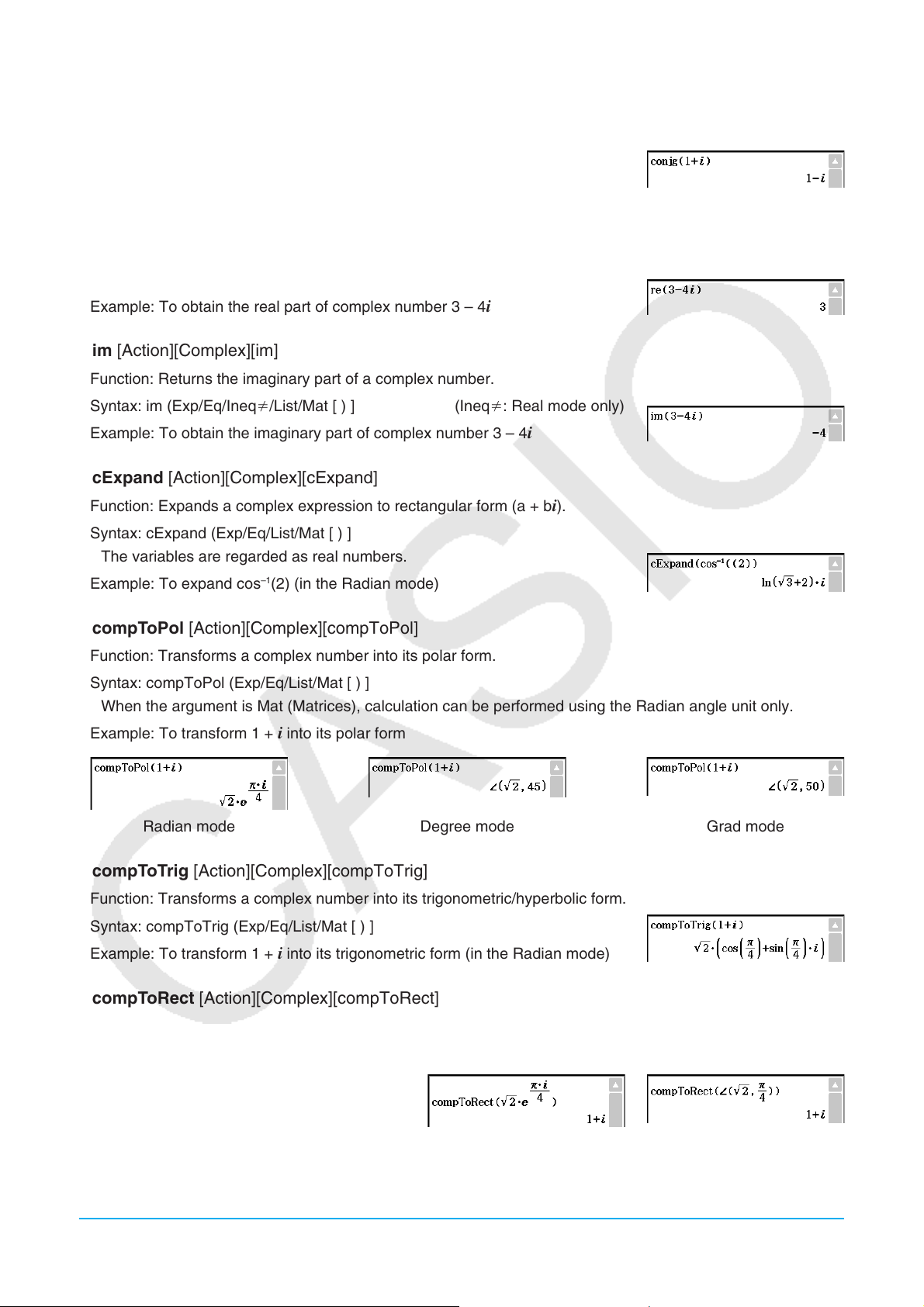
u conjg [Action][Complex][conjg]
Function: Returns the conjugate complex number.
Syntax: conjg (Exp/Eq/Ineq/List/Mat [ ) ] (Ineq: Real mode only)
Example: To obtain the conjugate of complex number 1 +
i
u re [Action][Complex][re]
Function: Returns the real part of a complex number.
Syntax: re (Exp/Eq/Ineq/List/Mat [ ) ] (Ineq: Real mode only)
Example: To obtain the real part of complex number 3 – 4
i
u im [Action][Complex][im]
Function: Returns the imaginary part of a complex number.
Syntax: im (Exp/Eq/Ineq/List/Mat [ ) ] (Ineq: Real mode only)
Example: To obtain the imaginary part of complex number 3 – 4
i
u cExpand [Action][Complex][cExpand]
Function: Expands a complex expression to rectangular form (a + bi).
Syntax: cExpand (Exp/Eq/List/Mat [ ) ]
• The variables are regarded as real numbers.
Example: To expand cos
–1
(2) (in the Radian mode)
u compToPol [Action][Complex][compToPol]
Function: Transforms a complex number into its polar form.
Syntax: compToPol (Exp/Eq/List/Mat [ ) ]
• When the argument is Mat (Matrices), calculation can be performed using the Radian angle unit only.
Example: To transform 1 +
Radian mode Degree mode Grad mode
i into its polar form
u compToTrig [Action][Complex][compToTrig]
Function: Transforms a complex number into its trigonometric/hyperbolic form.
Syntax: compToTrig (Exp/Eq/List/Mat [ ) ]
Example: To transform 1 +
i into its trigonometric form (in the Radian mode)
u compToRect [Action][Complex][compToRect]
Function: Transforms a complex number into its rectangular form.
Syntax: compToRect (⬔(
Example: To transform a complex number
into its rectangular form
r , ) or r · e^( · i ) form [ ) ]
Chapter 2: Main Application 68
Page 69
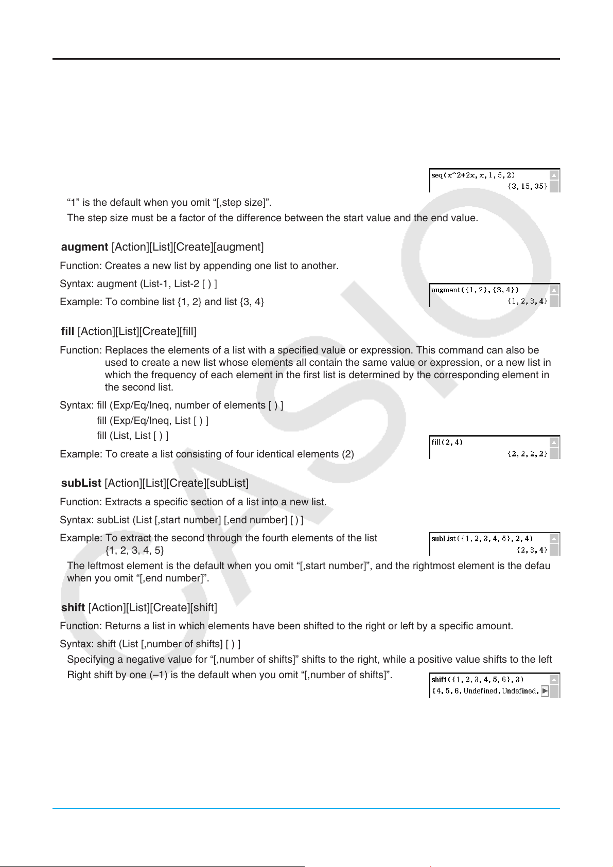
Using the List-Create Submenu
The [List][Create] submenu contains commands that are related to creating lists.
u seq [Action][List][Create][seq]
Function: Generates a list in accordance with a numeric sequence expression.
Syntax: seq (Exp, variable, start value, end value [,step size] [ ) ]
2
x
Example: To generate a list in accordance with the expression
when the start value is 1, the end value is 5, and the step size is 2
• “1” is the default when you omit “[,step size]”.
• The step size must be a factor of the difference between the start value and the end value.
u augment [Action][List][Create][augment]
Function: Creates a new list by appending one list to another.
Syntax: augment (List-1, List-2 [ ) ]
Example: To combine list {1, 2} and list {3, 4}
u fill [Action][List][Create][fill]
Function: Replaces the elements of a list with a specified value or expression. This command can also be
used to create a new list whose elements all contain the same value or expression, or a new list in
which the frequency of each element in the first list is determined by the corresponding element in
the second list.
+ 2x
Syntax: fill (Exp/Eq/Ineq, number of elements [ ) ]
fill (Exp/Eq/Ineq, List [ ) ]
fill (List, List [ ) ]
Example: To create a list consisting of four identical elements (2)
u subList [Action][List][Create][subList]
Function: Extracts a specific section of a list into a new list.
)
Syntax: subList (List [,start number] [,end number] [
Example: To extract the second through the fourth elements of the list
{1, 2, 3, 4, 5}
• The leftmost element is the default when you omit “[,start number]”, and the rightmost element is the default
when you omit “[,end number]”.
]
u shift [Action][List][Create][shift]
Function: Returns a list in which elements have been shifted to the right or left by a specific amount.
Syntax: shift (List [,number of shifts] [ ) ]
• Specifying a negative value for “[,number of shifts]” shifts to the right, while a positive value shifts to the left.
• Right shift by one (–1) is the default when you omit “[,number of shifts]”.
Example: To shift the elements of the list {1, 2, 3, 4, 5, 6} to the left by three
Chapter 2: Main Application 69
Page 70

u rotate [Action][List][Create][rotate]
Function: Returns a list in which the elements have been rotated to the right or to the left by a specific
amount.
Syntax: rotate (List [,number of rotations] [ ) ]
• Specifying a negative value for “[,number of rotations]” rotates to the right, while a positive value rotates to
the left.
Example: To rotate the elements of the list {1, 2, 3, 4, 5, 6} to the left by two
• Right rotation by one (–1) is the default when you omit “[,number of rotations]”.
u sortA [Action][List][Create][sortA]
Function: Sorts the elements of the list into ascending order.
Syntax: sortA (List [ ) ]
Example: To sort the elements of the list {1, 5, 3} into ascending order
u sortD [Action][List][Create][sortD]
Function: Sorts the elements of the list into descending order.
Syntax: sortD (List [ ) ]
Example: To sort the elements of the list {1, 5, 3} into descending order
u listToMat [Action][List][Create][listToMat]
Function: Transforms lists into a matrix.
Syntax: listToMat (List-1 [, List-2, ..., List-N] [ ) ]
Example: To transform the lists {3, 5} and {2, 4} into a matrix
u matToList [Action][List][Create][matToList]
• For information about matToList, see page 74.
Using the List-Statistics and List-Calculation Submenus
The [List][Statistics] and [List][Calculation] submenus contain commands related to list calculations.
u min [Action][List][Statistics][min]
Function: Returns the minimum value of an expression or the elements in a list.
Syntax: min (Exp/List-1[, Exp/List-2] [ ) ]
Example: To determine the minimum values of the elements in list {1, 2, 3}
u max [Action][List][Statistics][max]
Function: Returns the maximum value of an expression or the elements of a list.
)
Syntax: max (Exp/List-1[, Exp/List-2] [
Example: To determine the maximum value of the elements in list {1, 2, 3}
]
u mean [Action][List][Statistics][mean]
Function: Returns the mean of the elements in a list.
Syntax: mean (List-1[, List-2] [ ) ] (List-1: Data, List-2: Freq)
Example: To determine the mean of the elements in list {1, 2, 3}
Chapter 2: Main Application 70
Page 71
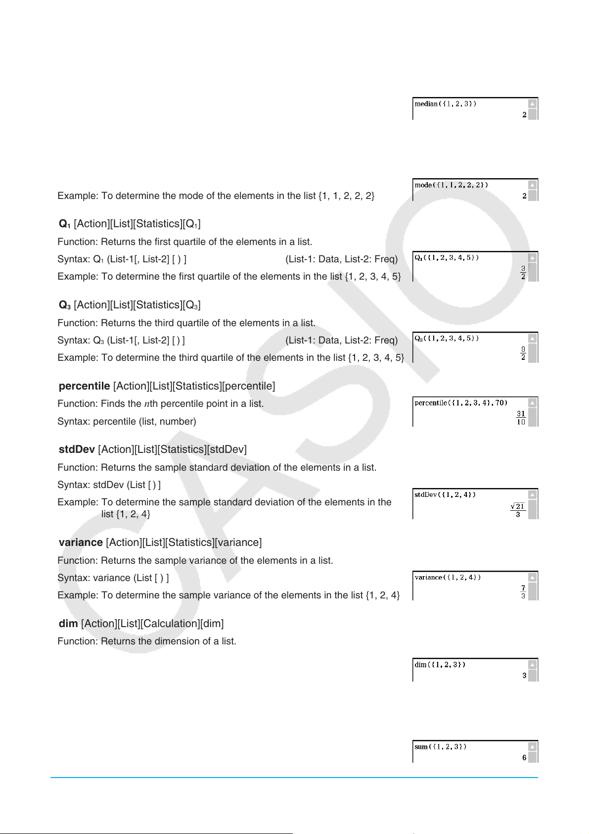
u median [Action][List][Statistics][median]
Function: Returns the median of the elements in a list.
Syntax: median (List-1[, List-2] [ ) ] (List-1: Data, List-2: Freq)
Example: To determine the median of the elements in the list {1, 2, 3}
u mode [Action][List][Statistics][mode]
Function: Returns the mode of the elements in a list. If there are multiple modes, they are returned in a list.
Syntax: mode (List-1[, List-2] [ ) ] (List-1: Data, List-2: Freq)
Example: To determine the mode of the elements in the list {1, 1, 2, 2, 2}
u Q1 [Action][List][Statistics][Q1]
Function: Returns the first quartile of the elements in a list.
Syntax: Q
Example: To determine the first quartile of the elements in the list {1, 2, 3, 4, 5}
(List-1[, List-2] [ ) ] (List-1: Data, List-2: Freq)
1
u Q3 [Action][List][Statistics][Q3]
Function: Returns the third quartile of the elements in a list.
Syntax: Q
Example: To determine the third quartile of the elements in the list {1, 2, 3, 4, 5}
(List-1[, List-2] [ ) ] (List-1: Data, List-2: Freq)
3
u percentile [Action][List][Statistics][percentile]
Function: Finds the n th percentile point in a list.
Syntax: percentile (list, number)
u stdDev [Action][List][Statistics][stdDev]
Function: Returns the sample standard deviation of the elements in a list.
)
Syntax: stdDev (List [
Example: To determine the sample standard deviation of the elements in the
list {1, 2, 4}
]
u variance [Action][List][Statistics][variance]
Function: Returns the sample variance of the elements in a list.
Syntax: variance (List [ ) ]
Example: To determine the sample variance of the elements in the list {1, 2, 4}
u dim [Action][List][Calculation][dim]
Function: Returns the dimension of a list.
Syntax: dim (List [ ) ]
Example: To determine the dimension of the list {1, 2, 3}
u sum [Action][List][Calculation][sum]
Function: Returns the sum of the elements in a list.
Syntax: sum (List-1[, List-2] [ ) ] (List-1: Data, List-2: Freq)
Example: To determine the sum of the elements in the list {1, 2, 3}
Chapter 2: Main Application 71
Page 72

u prod [Action][List][Calculation][prod]
Function: Returns the product of the elements in a list.
)
Syntax: prod (List-1[, List-2] [
Example: To determine the product of the elements in the list {1, 2, 3}
] (List-1: Data, List-2: Freq)
u cuml [Action][List][Calculation][cuml]
Function: Returns the cumulative sums of the elements in a list.
Syntax: cuml (List [ ) ]
Example: To determine the cumulative sums of the elements in the list {1, 2, 3}
u Alist [Action][List][Calculation][Alist]
Function: Returns a list whose elements are the differences between two adjacent elements in another list.
)
Syntax: Alist (List [
Example: To generate a list whose elements are the differences between two
adjacent elements in the list {1, 2, 4}
]
u percent [Action][List][Calculation][percent]
Function: Returns the percentage of each element in a list, the sum of which
is assumed to be 100.
)
Syntax: percent (List [
Example: To determine the percentage of each element in the list {1, 2, 3}
]
u polyEval [Action][List][Calculation][polyEval]
Function: Returns a polynomial arranged in the descending order of powers, so coefficients correspond
sequentially to each element in the input list.
Syntax: polyEval (List [,Exp/List] [
• “
x ” is the default when you omit “[,Exp/List]”.
Example: To create a second degree polynomial with the coefficients {1, 2, 3}
) ]
u sequence [Action][List][Calculation][sequence]
Function: Returns the lowest-degree polynomial that represents the sequence expressed by the input list.
When there are two lists, this command returns a polynomial that maps each element in the first list
to its corresponding element in the second list.
Syntax: sequence (List-1[, List-2] [,variable] [ ) ]
• “
x ” is the default when you omit “[,variable]”.
Example: To determine a polynomial for a sequence expressed by the list
{3, 5, 7, 9}
u sumSeq [Action][List][Calculation][sumSeq]
Function: Finds the lowest-degree polynomial that represents the sequence expressed by the input list and
returns the sum of the polynomial. When there are two lists, this command returns a polynomial that
maps each element in the first list to its corresponding element in the second list, and returns the
sum of the polynomial.
Chapter 2: Main Application 72
Page 73

Syntax: sumSeq (List-1[, List-2] [,variable] [ ) ]
• “
x ” is the default when you omit “[,variable]”.
Example: To determine the sum of a polynomial for a sequence expressed by
the list {3, 5, 7, 9}
Using the Matrix-Create Submenu
The [Matrix][Create] submenu contains commands related to creation of matrices.
u trn [Action][Matrix][Create][trn]
Function: Returns a transposed matrix.
Syntax: trn (Mat [ ) ]
Example: To transpose the matrix [[1, 2] [3, 4]]
u augment [Action][Matrix][Create][augment]
Function: Returns a matrix that combines two other matrices.
Syntax: augment (Mat-1, Mat-2 [ ) ]
Example: To combine the two matrices [[1, 2] [3, 4]] and [[5, 6]
[7, 8]]
u ident [Action][Matrix][Create][ident]
Function: Creates an identity matrix.
Syntax: ident (natural number [ ) ]
Example: To create a 2 × 2 identity matrix
u fill [Action][Matrix][Create][fill]
Function: Creates a matrix with a specific number of rows and columns, or replaces the elements of a matrix
with a specific expression.
Syntax: fill (Exp, number of rows, number of columns [ ) ]
fill (Exp, Mat [ ) ]
Example: To create a 2 × 3 matrix, all whose elements are 2
u subMat [Action][Matrix][Create][subMat]
Function: Extracts a specific section of a matrix into a new matrix.
Syntax: subMat (Mat [,start row] [,start column] [,end row] [,end column] [ ) ]
• “1” is the default when you omit “[, start row]” and “[, start column]”.
• The last row number is the default when you omit “[, end row]”.
• The last column number is the default when you omit “[, end column]”.
Example: To extract the section from row 2, column 2, to row 3, column
3 from the matrix [[1, 4, 7] [2, 5, 8] [3, 6, 9]]
u diag [Action][Matrix][Create][diag]
Function: Returns a one-row matrix containing the elements from the main diagonal of a square matrix.
Syntax: diag (Mat[ ) ]
Example: To extract the diagonal elements of the matrix [[1, 2] [3, 4]]
Chapter 2: Main Application 73
Page 74

u listToMat [Action][Matrix][Create][listToMat]
• For information about listToMat, see page 70.
u matToList [Action][Matrix][Create][matToList]
Function: Transforms a specific column of a matrix into a list.
Syntax: matToList (Mat, column number [ ) ]
Example: To transform column 2 of the matrix [[1, 2] [3, 4]] into a list
Using the Matrix-Calculation and Matrix-Row&Column Submenus
The [Matrix][Calculation] and [Matrix][Row&Column] submenus contain commands that are related to matrix
calculations.
u dim [Action][Matrix][Calculation][dim]
Function: Returns the dimensions of a matrix as a two-element list {number of rows, number of columns}.
)
Syntax: dim (Mat [
Example: To determine the dimensions of the matrix [[1, 2, 3] [4, 5, 6]]
u det [Action][Matrix][Calculation][det]
]
Function: Returns the determinant of a square matrix.
Syntax: det (Mat [ ) ]
Example: To obtain the determinant of the matrix [[1, 2] [4, 5]]
u norm [Action][Matrix][Calculation][norm]
Function: Returns the Frobenius norm of the matrix.
Syntax: norm (Mat [ ) ]
Example: To determine the norm of the matrix [[1, 2] [4, 5]]
u rank [Action][Matrix][Calculation][rank]
Function: Finds the rank of matrix.
The rank function computes the rank of a matrix by performing Gaussian
elimination on the rows of the given matrix. The rank of matrix A is the
number of non-zero rows in the resulting matrix.
Syntax: rank (Matrix)
u ref [Action][Matrix][Calculation][ref]
Function: Returns the row echelon form of a matrix.
Syntax: ref (Mat [ ) ]
Example: To obtain the row echelon form of the matrix [[1, 2, 3] [4, 5, 6]]
u rref [Action][Matrix][Calculation][rref]
Function: Returns the reduced row echelon form of a matrix.
Syntax: rref (Mat [ ) ]
Example: To obtain the reduced row echelon form of the matrix
[[2, –1, 3, 19] [1, 1, –5, –21] [0, 4, 3, 0]]
Chapter 2: Main Application 74
Page 75

u eigVl [Action][Matrix][Calculation][eigVl]
Function: Returns a list that contains the eigenvalue(s) of a square matrix.
Syntax: eigVl (Mat [ ) ]
Example: To obtain the eigenvalue(s) of the matrix [[3, 4] [1, 3]]
u eigVc [Action][Matrix][Calculation][eigVc]
Function: Returns a matrix in which each column represents an eigenvector of a square matrix.
• Since an eigenvector usually cannot be determined uniquely, it is standardized as follows to its norm, which
is 1:
When V = [
Syntax: eigVc (Mat [ ) ]
Example: To obtain the eigenvector(s) of the matrix [[3, 4] [1, 3]]
x 1, x 2, ..., xn ], (⎥ x 1⎥
2
+ ⎥ x 2⎥ 2 + .... + ⎥ xn ⎥ 2 ) = 1.
u LU [Action][Matrix][Calculation][LU]
Function: Returns the LU decomposition of a square matrix.
Syntax: LU (Mat, lVariableMem, uVariableMem [ ) ]
Example: To obtain the LU decomposition of the matrix [[1, 2, 3] [4, 5, 6] [7, 8, 9]]
• The lower matrix is assigned to the first variable L, while the upper
matrix is assigned to the second variable U.
To display the lower matrix To display the upper matrix
Lw
Uw
u QR [Action][Matrix][Calculation][QR]
Function: Returns the QR decomposition of a square matrix.
Syntax: QR (Mat, qVariableMem, rVariableMem [ ) ]
Example: To obtain the QR decomposition of the matrix [[1, 2] [3, 4]]
• The unitary matrix is assigned to variable Q, while the upper triangular
matrix is assigned to variable R.
To display the unitary matrix To display the upper triangular matrix
Qw
Rw
u swap [Action][Matrix][Row&Column][swap]
Function: Swaps two rows of a matrix.
Syntax: swap (Mat, row number-1, row number-2 [ ) ]
Example: To swap row 1 with row 2 of the matrix [[1, 2] [3, 4]]
Chapter 2: Main Application 75
Page 76
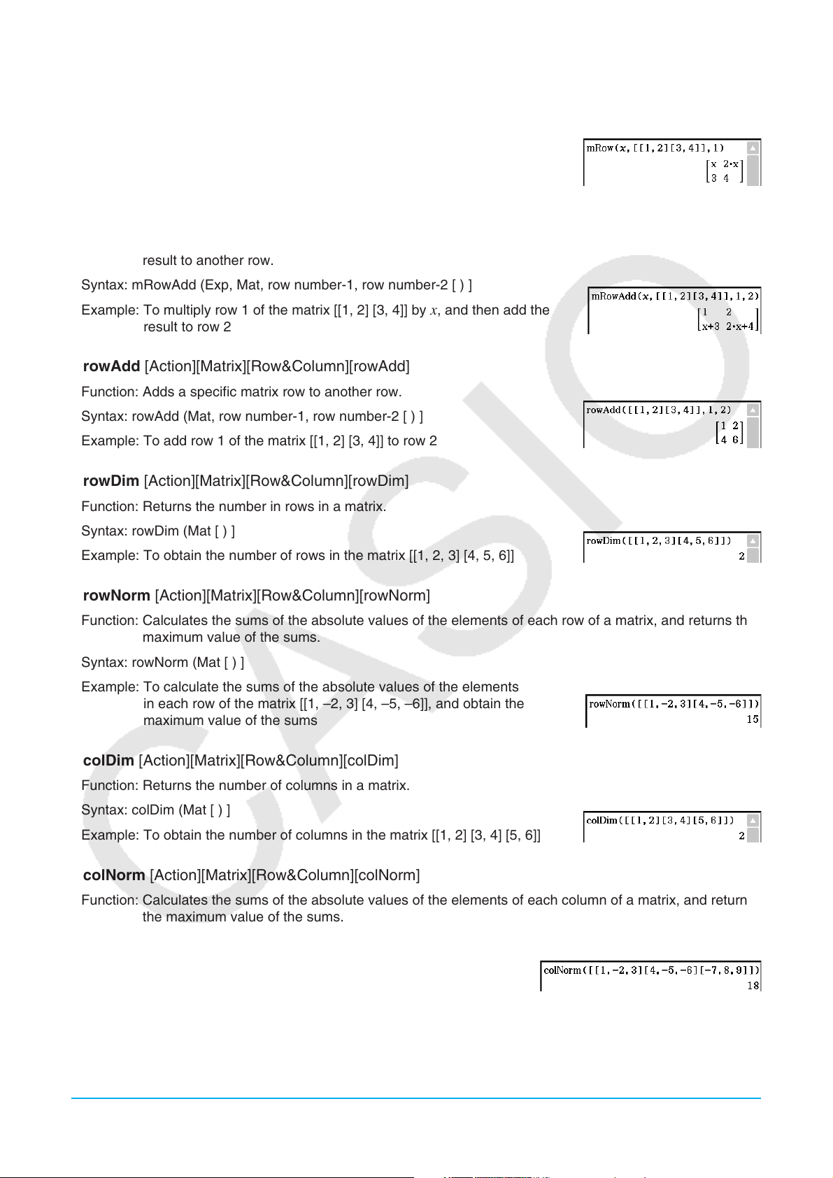
u mRow [Action][Matrix][Row&Column][mRow]
Function: Multiplies the elements of a specific row in a matrix by a specific
expression.
Syntax: mRow (Exp, Mat, row number [ ) ]
Example: To multiply row 1 of the matrix [[1, 2] [3, 4]] by
x
u mRowAdd [Action][Matrix][Row&Column][mRowAdd]
Function: Multiplies the elements of a specific row in a matrix by a specific expression, and then adds the
result to another row.
Syntax: mRowAdd (Exp, Mat, row number-1, row number-2 [ ) ]
Example: To multiply row 1 of the matrix [[1, 2] [3, 4]] by
result to row 2
x , and then add the
u rowAdd [Action][Matrix][Row&Column][rowAdd]
Function: Adds a specific matrix row to another row.
Syntax: rowAdd (Mat, row number-1, row number-2 [ ) ]
Example: To add row 1 of the matrix [[1, 2] [3, 4]] to row 2
u rowDim [Action][Matrix][Row&Column][rowDim]
Function: Returns the number in rows in a matrix.
Syntax: rowDim (Mat [ ) ]
Example: To obtain the number of rows in the matrix [[1, 2, 3] [4, 5, 6]]
u rowNorm [Action][Matrix][Row&Column][rowNorm]
Function: Calculates the sums of the absolute values of the elements of each row of a matrix, and returns the
maximum value of the sums.
Syntax: rowNorm (Mat [ ) ]
Example: To calculate the sums of the absolute values of the elements
in each row of the matrix [[1, –2, 3] [4, –5, –6]], and obtain the
maximum value of the sums
u colDim [Action][Matrix][Row&Column][colDim]
Function: Returns the number of columns in a matrix.
Syntax: colDim (Mat [ ) ]
Example: To obtain the number of columns in the matrix [[1, 2] [3, 4] [5, 6]]
u colNorm [Action][Matrix][Row&Column][colNorm]
Function: Calculates the sums of the absolute values of the elements of each column of a matrix, and returns
the maximum value of the sums.
Syntax: colNorm (Mat [ ) ]
Example: To calculate the sums of the absolute values of the elements
in each column of the matrix [[1, –2, 3][4, –5, –6][–7, 8, 9]],
and obtain the maximum value of the sums
Chapter 2: Main Application 76
Page 77

Using the Vector Submenu
The [Vector] submenu contains commands that are related to vector calculations.
• A vector is handled as a 1 × N matrix or N × 1 matrix.
• A vector in the form of 1 × N can be entered as [……] or [[……]].
Example: [1, 2], [[1, 2]]
• Vectors are considered to be in rectangular form unless ∠() is used to indicate an angle measure.
u augment [Action][Vector][augment]
Function: Returns an augmented vector [Mat-1 Mat-2].
Syntax: augment (Mat-1, Mat-2 [ ) ]
Example: To augment vectors [1, 2] and [3, 4]
u fill [Action][Vector][fill]
Function: Creates a vector that contains a specific number of elements, or replaces the elements of a vector
with a specific expression.
Syntax: fill (Exp, Mat [ ) ]
fill (Exp, 1, number of columns [ ) ]
Example: To replace the elements of the vector [1, 2] with
Example: To create a 1 × 3 (1 row, 3 columns) vector, all of whose elements
are “3”
x
u dim [Action][Vector][dim]
Function: Returns the dimension of a vector.
Syntax: dim (Mat [ ) ]
Example: To determine the dimension of the vector [1, 2, 3]
• The vector [1, 2, 3] is handled as a 1 × 3 matrix.
u unitV [Action][Vector][unitV]
Function: Normalizes a vector.
Syntax: unitV (Mat [ ) ]
• This command can be used with a 1 × N or N × 1 matrix only.
Example: To normalize the vector [1, 3, 5]
u angle [Action][Vector][angle]
Function: Returns the angle formed by two vectors.
Syntax: angle (Mat-1, Mat-2 [ ) ]
• This command can be used with a 1 × N or N × 1 matrix only.
Example: To determine the angle formed by vectors [1, 2] and [3, 4] (in the
Radian mode)
Chapter 2: Main Application 77
Page 78

u norm [Action][Vector][norm]
Function: Returns the norm of a vector.
Syntax: norm (Mat [ ) ]
Example: To obtain the norm of the vector [1, 2, 3]
u crossP [Action][Vector][crossP]
Function: Returns the cross product of two vectors.
Syntax: crossP (Mat-1, Mat-2 [ ) ]
• This command can be used with a 1 × N or N × 1 matrix only (N = 2, 3).
• A two-element matrix [a, b] or [[a], [b]] is automatically converted into a three-element matrix [a, b, 0] or
[[a], [b], [0]].
Example: To obtain the cross product of the two vectors [1, 3, 5] and [2, 4, 6]
u dotP [Action][Vector][dotP]
Function: Returns the dot product of two vectors.
Syntax: dotP (Mat-1, Mat-2 [ ) ]
• This command can be used with a 1 × N or N × 1 matrix only.
Example: To obtain the dot product of the two vectors [1, 3, 5] and [2, 4, 6]
u toRect [Action][Vector][toRect]
Function: Returns an equivalent rectangular form [ x y ] or [ x y z ].
Syntax: toRect (Mat [,natural number] [ ) ]
• This command can be used with a 1 × N or N × 1 matrix only (N = 2, 3).
• This command returns “
number” is 3.
• This command returns a rectangular form when you omit “natural number”.
Example: To transform the polar form ['2 , ∠(π/4)] into an equivalent
rectangular form (in the Radian mode)
x” when “natural number” is 1, “y” when “natural number” is 2, and “z” when “natural
u toPol [Action][Vector][toPol]
Function: Returns an equivalent polar form [ r ∠ ].
Syntax: toPol (Mat [,natural number] [ ) ]
• This command can be used with a 1 × 2 or 2 × 1 matrix only.
• This command returns “
• This command returns a polar form when you omit “natural number”.
Example: To transform the rectangular form [1, 2] into its equivalent polar
form
r” when “natural number” is 1, and “ ” when “natural number” is 2.
u toSph [Action][Vector][toSph]
Function: Returns an equivalent spherical form [ ρ ∠ ∠φ].
Syntax: toSph (Mat [,natural number] [ ) ]
• This command can be used with a 1 × 3 or 3 × 1 matrix only.
ρ
• This command returns “
number” is 3.
• This command returns a spherical form when you omit “natural number”.
” when “natural number” is 1, “ ” when “natural number” is 2, and “φ” when “natural
Chapter 2: Main Application 78
Page 79

Example: To transform the rectangular form [1, 1, 1] into its equivalent
spherical form (in the Radian mode)
u toCyl [Action][Vector][toCyl]
Function: Returns an equivalent cylindrical form [ r ∠ z ].
Syntax: toCyl (Mat [,natural number] [ ) ]
• This command can be used with a 1 × 3 or 3 × 1 matrix only.
• This command returns “
number” is 3.
• This command returns a cylindrical form when you omit “natural number”.
Example: To transform the rectangular form [1, 1, 1] into an equivalent
cylindrical form (in the Radian mode)
r” when “natural number” is 1, “ ” when “natural number” is 2, and “z” when “natural
Using the Equation/Inequality Submenu
The [Equation/Inequality] submenu contains commands that are related to equations and inequalities.
u solve [Action][Equation/Inequality][solve]
Function: Returns the solution of an equation or inequality.
)
Syntax: solve(Exp/Eq/Ineq [,variable] [
• “
x ” is the default when you omit “[,variable]”.
]
)
solve(Exp/Eq/Ineq,variable[, value, lower limit, upper limit] [
• “value” is an initially estimated value.
• This command is valid only for equations and expressions when “value” and the items following it
are included. In that case, this command returns an approximate value.
• A true value is returned when you omit “value” and the items following it. When, however, a true
value cannot be obtained, an approximate value is returned for equations only based on the
assumption that value = 0, lower limit = –
solve({Exp-1/Eq-1, ..., Exp-N/Eq-N}, {variable-1, ..., variable-N} [
• When “Exp” is the first argument, the equation Exp = 0 is presumed.
Example: To solve
Example: To solve simultaneous linear equations 3
You also could input the simultaneous equations shown in this example using the soft keyboard # key. The
following shows the required input syntax.
Exp-1/Eq-1
Exp-N/Eq-N variable-1, ..., variable-N
• The following shows the required key operation to input this example using the # key.
ax + b = 0 for x
∞, and upper limit = ∞.
x + 4 y = 5, 2 x – 3 y = –8
]
)
]
#dX+eY=fccX-dY=-ieX,Yw
• To input simultaneous equations with three or more unknowns, tap the # key when the cursor is in the
Exp-N/Eq-N input field. Each tap of # will add one more line for input of an equation.
Chapter 2: Main Application 79
Page 80

Note
For the solution, the solve function returns an expression or value for the expression (Exp/Eq) input as its
argument. The message “More solutions may exist” will appear on the display when a value is returned as the
solution, because there may be multiple solutions.
The solve function can return a maximum of 10 solutions in the case of values.
Example: To solve cos (
(Angle unit setting: Deg)
x ) = 0.5 for x (initial value: 0)
u dSolve [Action][Equation/Inequality][dSolve]
Function: Solves first, second or third order ordinary differential equations, or a system of first order
differential equations.
Syntax: dSolve(Eq, independent variable, dependent variable [, initial condition-1, initial condition-2][, initial
condition-3, initial condition-4][, initial condition-5, initial condition-6] [ ) ]
dSolve({Eq-1, Eq-2}, independent variable, {dependent variable-1, dependent variable-2} [, initial
condition-1, initial condition-2, initial condition-3, initial condition-4] [ ) ]
• If you omit the initial conditions, the solution will include arbitrary constants.
• Input all initial conditions equations using the syntax Var = Exp. Any initial condition that uses any other
syntax will be ignored.
Example: To solve a differential equation
Example: To solve the system of first order differential equations
independent variable, “ y ” and “ z ” are the dependent variables, and the initial conditions are y = 3
when x = 0, and z = '2 – 3 when x = 0
y ’ = x , where y = 1 when x = 0
y ’ = y + z , z ’ = y – z , where “ x ” is the
u rewrite [Action][Equation/Inequality][rewrite]
Function: Moves the right side elements of an equation or inequality to the left side.
Syntax: rewrite(Eq/Ineq/List [ ) ]
Example: To move the right side elements of
x + 3 = 5 x – x
2
to the left side
u exchange [Action][Equation/Inequality][exchange]
Function: Swaps the right-side and left-side elements of an equation or inequality.
Syntax: exchange(Eq/Ineq/List [ ) ]
Example: To swap the left-side and right-side elements of 3 > 5
x – 2 y
u eliminate [Action][Equation/Inequality][eliminate]
Function: Solves one equation with respect to a variable, and then replaces the same variable in another
expression with the obtained result.
Syntax: eliminate(Eq/Ineq/List-1, variable, Eq-2 [ ) ]
Example: To transform
2 x + 3 y = 5
y = 2 x + 3 to x =, and substitute the result into
Chapter 2: Main Application 80
Page 81

u absExpand [Action][Equation/Inequality][absExpand]
Function: Divides an absolute value expression into formulas without absolute value.
)
Syntax: absExpand(Eq/Ineq [
]
Example: To remove the absolute value from ⎜2
x – 3 ⎜ = 9
u andConnect [Action][Equation/Inequality][andConnect]
Function: Combines two equations or inequalities into a single expression.
Syntax: andConnect(Eq/Ineq-1, Eq/Ineq-2 [ ) ]
Example: To rewrite
x > –1 and x < 3 into a single inequality
u getRight [Action][Equation/Inequality][getRight]
Function: Extracts the right-side elements of an equation or inequality.
Syntax: getRight(Eq/Ineq/List [ ) ]
2
Example: To extract the right side elements of
y = 2 x
+ 3 x + 5
u getLeft [Action][Equation/Inequality][getLeft]
Function: Extracts the left-side elements of an equation or inequality.
Syntax: getLeft(Eq/Ineq/List [ ) ]
2
Example: To extract the left side elements of
y = 2 x
+ 3 x + 5
u and [Action][Equation/Inequality][Logic][and]
Function: Returns the result of the logical AND of two expressions.
Syntax: Exp/Eq/Ineq/List-1 and Exp/Eq/Ineq/List-2
2
x
Example: To obtain the result of the logical AND of
> 1 and x < 0
u or [Action][Equation/Inequality][Logic][or]
Function: Returns the result of the logical OR of two expressions.
Syntax: Exp/Eq/Ineq/List-1 or Exp/Eq/Ineq/List-2
Example: To obtain the result of the logical OR of
x = 3 or x > 2
u xor [Action][Equation/Inequality][Logic][xor]
Function: Returns the logical exclusive OR of two expressions.
Syntax: Exp/Eq/Ineq/List-1 xor Exp/Eq/Ineq/List-2
Example: To obtain the logical exclusive OR of
x < 2 xor x < 3
u not [Action][Equation/Inequality][Logic][not]
Function: Returns the logical NOT of an expression.
Syntax: not(Exp/Eq/Ineq/List [ ) ]
Example: To obtain the logical NOT of
x = 1
Chapter 2: Main Application 81
Page 82

Using the Assistant Submenu
The [Assistant] submenu contains two commands related to the Assistant mode.
Note that the following commands are valid in the Assistant mode only. For more information on the Assistant
mode see “Assistant Mode and Algebra Mode” on page 45.
u arrange [Action][Assistant][arrange]
Function: Collects like terms and arranges them in descending order, starting with the term that contains the
smallest coefficient.
Syntax: arrange (Exp/Eq/Ineq/List/Mat [ ) ]
Example: To arrange 2
x + 3 – 5 x + 8 y in the sequence of its variables
u replace [Action][Assistant][replace]
Function: Replaces the variable in an expression, equation or inequality with the value assigned to a variable
using the “store” command.
Syntax: replace (Exp/Eq/Ineq/List/Mat [ ) ]
Example: To replace
is assigned to s
s in the expression 3x + 2s, when the expression 2x + 1
u invert [Action][Transformation][invert]
Function: Inverts two variables in an expression.
Syntax: invert (Exp/Eq/Ineq/List [,variable-1, variable-2] [ ) ]
•
x and y are inverted when variables are not specified.
Example: To invert
x and y in the expression 2 x = y
u Clear_a_z
Function: Clears all single-character variable names (a–z and A–Z) in the
current folder.
Using the Distribution/Inv.Dist Submenu
The [Distribution/Inv.Dist] submenu includes functions related to each type of statistical calculation distribution
probability. The functions on this submenu perform the same calculations as the Distribution commands that
are available in the Statistics application and the Main, eActivity, and Program applications.
For information about the numeric expressions used in calculations, see “Distributions” on page 145.
For information about the meanings of the variables used in the syntaxes of the functions presented in this
section, and the system variables that store the values obtained as calculation results, see “Input and Output
Terms” on page 148.
Specifying Arguments within the Distribution Function
You can specify either values or list data for any of the arguments within the Distribution function. The normPDf
function (page 83) syntax (normPDf( x , , )) that returns normal probability density can be used to perform the
calculations shown below. The “Number Format” setting is “Fix 2” for all calculation results.
normPDf(1, 1, 0) = 0.24
normPDf({1, 2}, 1, 0) = {0.24, 0.05}
normPDf(1, {1, 2}, 0) = {0.24, 0.18}
normPDf({1, 2},{1, 2}, 0) = {0.24, 0.12}
normPDf({1, 2},{1, 2},{1, 0}) = {0.40, 0.12}
Chapter 2: Main Application 82
Page 83

The following explains how to specify list data in arguments and how calculation results are output.
(a) Specifying list data for a single argument
• Basically, you can specify any list you like, but the each of the elements in the list must be in accordance
with the conditions required by the argument of the function being used.
• Calculation is performed on each element within the list and results are output as shown below.
x , {
normPDf(
= {<normPDf(
, 2}, )
1
x ,
, ) calculation result>, <normPDf( x , 2, ) calculation result>}
1
(b) Specifying list data for multiple arguments
• In this case, all of the lists must have the same number of elements. Otherwise an Invalid Dimension error
will occur.
• Calculation is performed on each element within the list and results are output as shown below.
x
normPDf({
= {<normPDf(
, x 2}, { 1, 2}, )
1
x
, 1, ) calculation results>, <normPDf( x 2, 2, ) calculation results>}
1
Assignment of List Data Calculation Results to Variables
Using the list data in the argument of the Distribution function causes calculation results to be output as list
data, which is assigned as-is to the “ans” variable.
In addition to the “ans” variable, calculations that use the Distribution function causes calculation results also
to be assigned to certain system variables. For example, the normal probability density variable returned by
normPDf is assigned to system variable prob . Only the last element of the list data will be assigned to a system
variable as a calculation result.
In the distribution function explanations below, the names of the functions to which calculation results are
assigned are shown under “Calculation Result Output”.
u normPDf [Action][Distribution/Inv.Dist][Continuous][normPDf]
Function: Returns the normal probability density for a specified value.
x [,
σ
Syntax: normPDf(
• When
σ
and μ are skipped, σ = 1 and μ = 0 are used.
Calculation Result Output:
, μ)]
prob
Example: To determine the normal probability density when x = 37.5,
σ
= 2, μ = 35
u normCDf [Action][Distribution/Inv.Dist][Continuous][normCDf]
Function: Returns the cumulative probability of a normal distribution between a lower bound and an upper
bound.
σ
Syntax: normCDf(lower value, upper value[,
• When
Calculation Result Output:
σ
and μ are skipped, σ = 1 and μ = 0 are used.
prob , z Low, z Up
Example: To determine the normal probability density when lower bound
value = −
∞, upper bound value = 36,
, μ)]
σ
= 2, μ = 35
u invNormCDf [Action][Distribution/Inv.Dist][Inverse][invNormCDf]
Function: Returns the boundary value(s) of a normal cumulative distribution probability for specified values.
Syntax: invNormCDf([tail setting, ]area value[,
• When
σ
and μ are skipped, σ = 1 and μ = 0 are used.
σ
, μ)]
Chapter 2: Main Application 83
Page 84

• “tail setting” displays the probability value tail specification, and Left, Right, or Center can be specified. Enter
the following values or letters to specify:
Left: −1, “L”, or “l”
Center: 0, “C”, or “c”
Right: 1, “R”, or “r”
When input is skipped, “Left” is used.
• When one argument is omitted (resulting in three arguments), Tail=Left.
μ
• When two arguments are omitted (resulting in two arguments), Tail=Left,
• When three arguments are omitted (resulting in one argument), Tail=Left,
• When “tail setting” is Center, the lower bound value is returned.
=0.
σ
=1, μ =0.
Calculation Result Output:
Example: To determine the upper bound value when tail setting = Left, area
value = 0.7, σ = 2, μ = 35
x
InvN, x2InvN
1
u tPDf [Action][Distribution/Inv.Dist][Continuous][tPDf]
Function: Returns the Student’s t probability density for a specified value.
Syntax: tPDf(
Calculation Result Output:
Example: To determine the Student’s t probability density when x = 2, df = 5
x, df [ ) ]
prob
u tCDf [Action][Distribution/Inv.Dist][Continuous][tCDf]
Function: Returns the cumulative probability of a Student’s t distribution between a lower bound and an upper
bound.
Syntax: tCDf(lower value, upper value,
Calculation Result Output: prob, tLow, tUp
Example: To determine the Student’s
lower value = 1.5, upper value = ∞, df = 18
df [ ) ]
t distribution probability when
u invTCDf [Action][Distribution/Inv.Dist][Inverse][invTCDf]
Function: Returns the lower bound value of a Student’s t cumulative distribution probability for specified
values.
Syntax: invTCDf(
Calculation Result Output: xInv
Example: To determine the lower bound value when
prob, df [ ) ]
prob = 0.0754752,
df = 18
u chiPDf [Action][Distribution/Inv.Dist][Continuous][chiPDf]
Function: Returns the χ2 probability density for specified values.
Syntax: chiPDf(
Calculation Result Output: prob
Example: To determine the χ2 probability density when x = 2, df = 4
x, df [ ) ]
Chapter 2: Main Application 84
Page 85

u chiCDf [Action][Distribution/Inv.Dist][Continuous][chiCDf]
Function: Returns the cumulative probability of a χ2 distribution between a lower bound and an upper bound.
Syntax: chiCDf(lower value, upper value,
Calculation Result Output:
Example: To determine the χ2 probability when lower value = 2.7,
upper value = ∞, df = 4
prob
df [ ) ]
u invChiCDf [Action][Distribution/Inv.Dist][Inverse][invChiCDf]
Function: Returns the lower bound value of a χ2 cumulative distribution probability for specified values.
Syntax: invChiCDf(
Calculation Result Output:
Example: To determine the lower bound value when prob = 0.6092146, df = 4
prob, df [ ) ]
xInv
u fPDf [Action][Distribution/Inv.Dist][Continuous][fPDf]
Function: Returns the F probability density for a specified value.
Syntax: fPDf(
Calculation Result Output:
Example: To determine the F probability density when x = 1.5, n : df = 24,
x , n : df , d : df [ ) ]
prob
d : df = 19
u fCDf [Action][Distribution/Inv.Dist][Continuous][fCDf]
Function: Returns the cumulative probability of an F distribution between a lower bound and an upper bound.
Syntax: fCDf(lower value, upper value,
Calculation Result Output:
Example: To determine the F distribution probability when lower value = 1.5,
upper value = ∞, n : df = 24, d : df = 19
prob
n : df , d : df [ ) ]
u invFCDf [Action][Distribution/Inv.Dist][Inverse][invFCDf]
Function: Returns the lower bound value of an F cumulative distribution probability for specified values.
Syntax: invFCDf(
Calculation Result Output:
Example: To determine the lower bound value when
d : df = 19
prob , n : df , d : df [ ) ]
x Inv
prob = 0.1852, n : df = 24,
u binomialPDf [Action][Distribution/Inv.Dist][Discrete][binomialPDf]
Function: Returns the probability in a binomial distribution that the success will occur on a specified trial.
Syntax: binomialPDf(
Calculation Result Output: prob
Example: To determine the binomial probability when x = 5, numtrial value = 3,
pos = 0.63
x , numtrial value, pos [ ) ]
Chapter 2: Main Application 85
Page 86

u binomialCDf [Action][Distribution/Inv.Dist][Discrete][binomialCDf]
Function: Returns the cumulative probability in a binomial distribution that the success will occur between
specified lower value and upper value.
Syntax: binomialCDf(lower value, upper value, numtrial value,
Calculation Result Output:
Example: To determine the binomial cumulative probability when lower value
= 2, upper value = 5, numtrial value = 3, pos = 0.63
prob
pos [ ) ]
u invBinomialCDf [Action][Distribution/Inv.Dist][Inverse][invBinomialCDf]
Function: Returns the minimum number of trials of a binomial cumulative probability distribution for specified
values.
Syntax: invBinomialCDf(
Calculation Result Output:
prob , numtrial value, pos [ ) ]
x Inv, ½ x Inv
Important!
When executing the invBinomialCDf, invPoissonCDf, invGeoCDf, or
invHypergeoCDf function, the ClassPad uses the specified prob value and
the value that is one less the prob value minimum number of significant digits
prob value) to calculate minimum number of trials values. The results
(½
are assigned to the system variables
and ½ xInv (calculation result using ½ prob ). The function always returns the
xInv value only. However, when the xInv and ½ xInv values are different, the
warning message shown nearby appears showing both values.
The calculation results of the function are integers. Accuracy may be reduced
when the first argument has 10 or more digits. Note that even a slight difference in calculation accuracy
affects calculation results. If a warning message appears, check the displayed values.
xInv (calculation result using prob )
Example: To determine the minimum number of trials when
numtrial value = 5, pos = 0.63
prob = 0.609,
u poissonPDf [Action][Distribution/Inv.Dist][Discrete][poissonPDf]
Function: Returns the probability in a Poisson distribution that the success will occur on a specified trial.
Syntax: poissonPDf(
Calculation Result Output:
Example: To determine the Poisson probability when x = 10, = 6
x , [ ) ]
prob
u poissonCDf [Action][Distribution/Inv.Dist][Discrete][poissonCDf]
Function: Returns the cumulative probability in a Poisson distribution that the success will occur between
specified lower value and upper value.
Syntax: poissonCDf(lower value, upper value, [ ) ]
Calculation Result Output:
Example: To determine the Poisson cumulative probability when lower
value = 2, upper value = 3, = 2.26
prob
u invPoissonCDf [Action][Distribution/Inv.Dist][Inverse][invPoissonCDf]
Function: Returns the minimum number of trials of a Poisson cumulative probability distribution for specified
values.
Syntax: invPoissonCDf(
Calculation Result Output: x Inv, ½ x Inv
prob , [ ) ]
Chapter 2: Main Application 86
Page 87

Important!
See “Important!” under “invBinomialCDf” on page 86.
Example: To determine the minimum number of trials when
= 2.26
prob = 0.8074,
u geoPDf [Action][Distribution/Inv.Dist][Discrete][geoPDf]
Function: Returns the probability in a geometric distribution that the success will occur on a specified trial.
Syntax: geoPDf( x , pos [ ) ]
Calculation Result Output:
Example: To determine the geometric probability when x = 6, pos = 0.4
prob
u geoCDf [Action][Distribution/Inv.Dist][Discrete][geoCDf]
Function: Returns the cumulative probability in a geometric distribution that the success will occur between
specified lower value and upper value.
Syntax: geoCDf(lower value, upper value, pos [ ) ]
Calculation Result Output:
Example: To determine the geometric probability when lower value = 2,
upper value = 3, pos = 0.5
prob
u invGeoCDf [Action][Distribution/Inv.Dist][Inverse][invGeoCDf]
Function: Returns the minimum number of trials of a geometric cumulative probability distribution for specified
values.
Syntax: invGeoCDf(
Calculation Result Output:
prob , pos [ ) ]
x Inv, ½ x Inv
Important!
See “Important!” under “invBinomialCDf” on page 86.
Example: To determine the minimum number of trials when
prob = 0.875,
pos = 0.5
u hypergeoPDf [Action][Distribution/Inv.Dist][Discrete][hypergeoPDf]
Function: Returns the probability in a hypergeometric distribution that the success will occur on a specified
trial.
Syntax: hypergeoPDf(
Calculation Result Output:
Example: Determine the hypergeometric probability when x = 1, n = 5,
M = 10, N = 20.
x , n , M , N [ ) ]
prob
u hypergeoCDf [Action][Distribution/Inv.Dist][Discrete][hypergeoCDf]
Function: Returns the cumulative probability in a hypergeometric distribution that the success will occur
between specified lower value and upper value.
Syntax: hypergeoCDf(lower value, upper value,
n , M , N [ ) ]
Calculation Result Output:
Example: Determine the hypergeometric cumulative distribution when lower
value = 0, upper value = 1, n = 5, M = 10, N = 20.
prob
Chapter 2: Main Application 87
Page 88

u invHypergeoCDf [Action][Distribution/Inv.Dist][Inverse][invHypergeoCDf]
Function: Returns the minimum number of trials of a hypergeometric cumulative distribution for specified
values.
Syntax: invHypergeoCDf(
Calculation Result Output:
prob , n , M , N [ ) ]
x Inv, ½ x Inv
Important!
See “Important!” under “invBinomialCDf” on page 86.
Example: To determine the minimum number of trials when
M = 10, N = 20
prob = 0.3, n = 5,
Using the Financial Submenu
The [Financial] submenu contains commands that are related to financial calculations.
For information about the functions included in this submenu, see “11-4 Financial Calculation Functions”.
Using the Command Submenu
u Define
Function 1: Defines function and registers it with Graph Editor.
Syntax 1: Define{ y1(x) − y100(x) ; x1(y) − x100(y) ; yt1(t) − yt100(t) ; xt1(t) − xt100(t) ;
r1() − r100()} = <expression>
Example: To define the function
Graph Editor
y = sin(x) and assign it to line “y3” of the
Function 2: Creates a user-defined function.
For more information, see “12-3 User-defined Functions”.
u DispStat
Function: Displays previous statistical calculation results.
For more information, see “DispStat” on page 202 and the examples
Statistical Graphing and Calculation Functions in a Program” on page 218.
1208 through 1210 under “Including
u Clear_a_z
Function: Clears all single-character variables.
For more information, see “Clear_a_z” on page 82.
u DelVar
Function: Deletes a specified variable.
For more information, see “DelVar” on page 201.
u Clear All Variables
Function: Clear variables that contain numbers, list and matrices.
Chapter 2: Main Application 88
Page 89

2-8 Using the Interactive Menu
The [Interactive] menu includes most of the commands that are on the [Action] menu. Selecting a command on
the [Action] menu will simply input the command.
With the [Interactive] menu, you drag the stylus across existing input in the work area and then select a
command. This encloses the highlighted expression with the command and opens a dialog box if more
arguments are needed. When you select an [Interactive] menu item without highlighting an expression first, a
dialog box will open prompting you for the necessary arguments.
Tip
• Operation of the following [Interactive] menu commands is identical to the same commands on the [Action] menu. For
information about using these commands, see “2-7 Using the Action Menu”.
[Transformation], [Advanced], [Calculation], [Complex], [List]-[Create], [List]-[Statistics], [List]-[Calculation], [Matrix]-
[Create], [Matrix]-[Calculation], [Matrix]-[Row&Column], [Vector], [Equation/Inequality], [Assistant], [Distribution/Inv.Dist],
[Financial], Define
• The “DispStat”, “Clear_a_z,” and “DelVar” commands of the [Action] menu’s [Command] submenu are not included on the
[Interactive] menu.
Interactive Menu Example
[Interactive] menu operations come in handy in the following cases.
• When you want to use a command on an expression you are calculating
• When you want to use a command that requires multiple arguments
0234 To factorize the expression x 3 – 3 x 2 + 3 x – 1
0235 To obtain the definite integral of x 2 + 2 x , 1 s x s 2
Using the “apply” Command
The “apply” command is included on the [Interactive] menu only. You can use this command to execute only a
specific part of an expression and display its result.
0236 To calculate the result of diff(sin( x ), x ) × cos( x ) + sin( x ) × diff(cos( x ), x ), and then calculate only part of
the expression
Note: This example assumes that your ClassPad is configured with the following mode settings:
Algebra, Complex, Radian, Descending Order.
2-9 Using the Main Application in Combination with
Other Applications
You can access the windows of other ClassPad applications from the Main application and perform copy,
paste, drag and drop, and other operations between them.
Tip
• Copying data that includes color information from another application and pasting it into the Main application will cause
the color information to be disregarded, and the pasted data will become black. This is also true when dragging data from
another application to the Main application.
• Copying data in the Main application and pasting it into another application will cause the pasted data to be displayed in
accordance with the other application’s color settings. This is also true when dragging data from the Main application to
another application.
Chapter 2: Main Application 89
Page 90

Using Another Application’s Window
u To open another application’s window
1. Tap the right most toolbar down arrow button.
• This displays a palette of application icons.
Graph Editor
Graph
Spreadsheet
Stat Editor
Probability
Verify
2. Tap the button that corresponds to the window you want to display.
• This causes the window that corresponds to the button you tap to appear in the lower window.
u To close another application’s window
1. Tap anywhere inside of the window you would like to close.
Geometry
Conics Graph
Conics Editor
Financial
Differential Equation Editor
Sequence Editor
Numeric Solver
2. Tap the C button in the upper right corner, or tap O and then [Close].
• The Main application work area expands to fill the entire display.
Tip
• Even if you used the icon panel r icon to expand the lower window to fill the entire display, tapping O and then [Close]
closes it and returns to the work area window.
• Nothing happens if you tap O and then [Close] while the work area window is active.
u To copy an expression in the work area and paste it into the Graph Editor window
0237 To copy “ x 2 – 1” in the work area and paste it into the Graph Editor window
• For more information about the Graph Editor window, see Chapter 3.
u To graph a function by dragging it from the work area to the Graph window
0238 To graph the expression “ x 2 – 1”, which has already been input into the work area
• As can be seen in this example, a graph can be drawn by dropping an expression in the form of
f ( x ) into the
Graph window.
Using the Stat Editor Window
You can use the Stat Editor window to create new LIST variables and edit existing LIST variables. You can also
use the Stat Editor window to specify a LIST variable’s name and display its contents.
u To use a LIST variable with data input using Stat Editor to perform a calculation in the work
area
0239 To input data into “list1” and “list2” using Stat Editor, and then perform the calculation list1+list2 in the
work area
• list1 through list6 are LIST type system variables. For more information, see “Main Memory Data Types”
(page 26).
Chapter 2: Main Application 90
Page 91

• For information about inputting and editing list data using the Stat Editor, see Chapter 7.
u To use Stat Editor to recall a LIST variable created in the work area
0240 Continuing from example 0239 , to use Stat Editor to recall list variable “test”, which was created in the
work area
Using the Geometry Window
When there is a Geometry window on the display, you can drag values and expressions to the Geometry
window to draw the graph or figure of the value or expression. You can also drag a figure from the Geometry
window to the work area, which displays the corresponding expression or value.
u To drag an expression from the work area to the Geometry window
0241 To input the expression x2/52 + y2/22 = 1 in the work area, and then drag it to the Geometry window
Tip: The following table shows the types of expressions you can drop into the Geometry window. When the expression is
not recognized, Geometry displays it as text.
Dropping this into the Geometry window: Displays this:
Linear equation in
Equation of circle in
Equation of ellipse in
Equation of hyperbola in
2-dimensional vector (2 rows × 1 column format) A point
Equation
2 ×
y = f ( x)
n matrix, n t 3
x and y
x and y
x and y
x and y
n × 2 matrix, n t 3
An infinite line
A circle
An ellipse
A hyperbola
A curve
A polygon (each column represents a vertex of the
polygon)
An open polygon
u To drag a figure from the Geometry window to the work area
0242 To drag a point, circle, point and its image from the Geometry window to the work area
• For details about Geometry window operations, see Chapter 8.
Tip: The following shows what happens when you drag a figure from the Geometry window to the work area.
Dropping this into the work area: Displays this:
Point Coordinates as a vector (2 × 1 matrix)
Line Equation of the line
Vector An ordered pair (head of vector assuming the tail is at the
origin)
Circle, Arc, Ellipse, Function, or Curve Corresponding equation
Polygon
Open Polygon (Created by Animation)
Line Pair Simultaneous equations for the pair
A point and its image under a transformation Matrix expression for the transformation
2 ×
n matrix
n × 2 matrix
Chapter 2: Main Application 91
Page 92

2-10 Using Verify
Verify provides you with a powerful tool to check whether your numeric or algebraic manipulations are correct.
Verify will assist you in simplifying an expression by verifying whether or not the expression you entered is
equivalent to your original expression. If it is, you will get a pleasant response; if not, you will need to correct
your mistake before continuing.
u To start up Verify
1. On the work area window, tap the right most
toolbar down arrow button.
2. On the icon palette that appears, tap W.
u Verify window menus and buttons
• Clear the Verify window ............................................................................... File - New, Edit - Clear All or O
• Open or save a file ............................................................................................File - Open, File - Save or {
• Specify the complex number calculation range for Verify ........................................................................... T
• Specify the real number calculation range for Verify ..................................................................................Y
• Specify the positive real number calculation range for Verify ..................................................................... U
Left-side expression
Right-side expression
• Verify the equation starting from the first line ..............................................................................................!
• Verify the equation starting from the current line ........................................................................................"
0243 To factor 50 completely
0244 Continuing from example 0243 , to rewrite x 2 + 1 in factored form
2-11 Using Probability
You can use Probability to simulate the following.
• The die faces that will appear when a single die is thrown a specified number of times (1 Die)
• The sum of the data of dice faces that will appear when a pair of dice is thrown a specified number of times (2
Dice +)
• The product of the data of dice faces that will appear when a pair of dice is thrown a specified number of
times (2 Dice ½)
• When any number of balls labeled A, B, C, D, E, and F are placed into a box, data about how many times
each ball will be drawn within a specified number of draws (Container)
You can specify any integer from 1 to 20 as the number of die faces.
Probability dialog box
Probability window
(Trial information and result)
Chapter 2: Main Application 92
Page 93

u To start up Probability
1. On the work area window, tap the right most toolbar down arrow button.
2. On the icon palette that appears, tap P. This will display an initial Probability dialog box.
u Probability window menus and buttons
• Clear the Probability window (and display the Probability dialog box) ......... File - New, Edit - Clear All or O
• Display the Probability dialog box and try the probability emulation
(the trial result will be added to the end of the current file) ...............................................Edit - Add or P
• Open or save a file ............................................................................................File - Open, File - Save or {
• Delete the currently selected trial data ......................................................................................... Edit - Delete
• Show the selected result as a frequency distribution table (in matrix form) ....................Display - Distribution
• Show the selected result as sample data (in list form) ................................................. Display - Sample Data
0245 To obtain the sum data when a two six-sided die are thrown 50 times
0246 After putting 10 A-balls, 20 B-balls, and 30 C-balls into a box, determine how many times each type of
ball will be drawn when there is a total of 50 draws. Each time a ball is drawn, it should be replaced into
the box before the next draw.
Tip: Under initial default settings, trial results are shown as a frequency distribution table in matrix form. Selecting
distribution table results and selecting [Sample Data] on the [Display] menu will change them to sample data in list
form. Conversely, selecting sample data results and selecting [Distribution] on the [Display] menu will change them to
distribution table results.
Distribution table (matrix form)
Sample data (list form)
2-12 Running a Program in the Main Application
You can run a program in the Main application or the eActivity application.
Syntax: Folder name\Program name(parameter)
• You do not need to specify the folder name if the program you want to run is in the current folder. If you leave
ClassPad configured with its initial default settings, the current folder for both the Program application and the
Main application is the “main” folder, so you normally do not need to specify a folder name.
• Unless you change it, the current folder of the eActivity application is the “eAct” folder, so you always need
to specify the folder name. If you want to run a program that is in the “main” folder, input “main\Program
name(parameter)”.
Chapter 2: Main Application 93
Page 94

Important!
If the program command “Pause” is used in a program, it is ignored when the program is called from Main or
eActivity.
Program Main application eActivity application
0247 To run the program named OCTA that we created and stored under “Creating a Program” (page 190) from
the Main application, and determine the surface area and volume of a regular octahedron with a side
length of 20 cm
Chapter 2: Main Application 94
Page 95

Chapter 3: Graph & Table Application
The Graph & Table application allows you to input and graph rectangular coordinate equations (or inequalities),
polar coordinate equations, and parametric expressions. After you graph an expression, you can perform
various graph-based analytical operations, such as determining the points of intersection of two graphs, point of
inflection, and definite integral for a particular range of a parabola or other figure.
When you start up the Graph & Table application, two windows appear
on the display: 1 the Graph Editor window and 2 the Graph window.
• A Graph Editor sheet can contain up to 20 functions. You can have up
to 100 functions stored in the Graph Editor at one time. Functions stored
in the Graph Editor can be graphed on the Graph window.
• You can also use a function on the Graph Editor window to generate a
number table or a summary table. Number tables and summary tables
are displayed in a Table window.
• The Graph window and Table window have a message box along the
bottom that can display expressions and values, or they can be used for
input and editing.
1
2
Message box
Graph & Table Application-Specific Menus and Buttons
Graph Editor window
• Open batch saved data in the Graph Editor window ............................................. File - Open Graph Memory
• Save all of the expressions on the Graph Editor window .......................................File - Save Graph Memory
• Select the entire expression you are editing ........................................................................... Edit - Select All
• Clear all of the expressions from the Graph Editor window ...................................................... Edit - Clear All
• Input a rectangular coordinate type function ...................................................................Type -
• Input a polar coordinate type function .............................................................................Type -
• Input a parametric function ......................................................................................Type - ParamType or g
• Input an
• Input a rectangular coordinate type inequality
• Input an
• Input two functions in a list and shade between them .............................................Type - ShadeType or y
• Display the Dynamic Graph dialog box (page 113) ........................................................ a - Dynamic Graph
x equality ...........................................................................................................Type - x=Type or h
............................................... Type - Inequality -
y>Type, y<Type, ytType, ysType or j, l, ', X
x inequality ...................... Type - Inequality - x>Type, x<Type, xtType, xsType or k, ;, Z, C
y=Type or d
r=Type or f
• Display the Draw Shade dialog box (page 99) ......................................................................a - Draw Shade
• Use a built-in function template for graphing ................................................................................ a - Built-In
• Delete all of the expressions on the active sheet ......................................................a - Sheet - Clear Sheet
• Return the active sheet name to its initial default ..................................................a - Sheet - Default Name
Chapter 3: Graph & Table Application 95
Page 96

• Graph the selected function(s) ....................................................................................................................$
• Generate a summary table for the selected function ..................................................................................4
• Display the View Window dialog box to configure Graph window settings ................................................. 6
• Display the Table Input dialog box for configuring settings .........................................................................8
• Generate a table for the selected function .................................................................................................. #
Graph window
• Clear all of the Graph window contents .................................................................................... Edit - Clear All
• Perform a zoom operation (page 103) ....................................................................................................Zoom
• Display the coordinates at a particular point on a graph ..............................................Analysis - Trace or =
• Insert a point, a graphic, or text into an existing graph (page 110) ...................................... Analysis - Sketch
• Perform a G-Solve operation (page 112) ........................................................................... Analysis - G-Solve
• Modify a graph by changing the value of a coefficient ..........................................................Analysis - Modify
• Open the image of a graph ................................................................................................. a - Open Picture
• Save a graph as image data ................................................................................................ a - Save Picture
• Clear the image of a graph ..................................................................................................a - Clear Picture
• Adjust the lightness of the graph screen background image placed
by the “Open Picture” command ........................................................................................... a - Fade I/O
• Display the Dynamic Graph dialog box ........................................................................... a - Dynamic Graph
• Display the Draw Shade dialog box ......................................................................................a - Draw Shade
• Use a built-in function template for graphing (page 104) .............................................................. a - Built-In
• Re-draw a graph ......................................................................................................................... a - ReDraw
• Make the Graph Editor window active ........................................................................................................!
• Generate a number table for an existing graph ..........................................................................................#
• Display the Table Input dialog box for configuring settings .........................................................................8
• Generate a summary table for an existing graph ........................................................................................4
Table window
• Clear all of the Table window contents ..................................................................................... Edit - Clear All
• Delete a row from a table .........................................................................................................T-Fact - Delete
• Insert a row into a table ............................................................................................................. T-Fact - Insert
• Add a row after the currently selected row ..................................................................................T-Fact - Add
• Draw a connect type graph using a generated table ..............................................Graph - G-Connect or $
• Draw a plot type graph using a generated table ............................................................ Graph - G-Plot or !
• Save the contents of a table to a list .....................................................................................a - Table to List
• Re-generate a table based on current table settings ..................................................................a - ReTable
• Delete the displayed table .................................................................................................... a - Delete Table
• Move the pointer to the location on a graph that corresponds
to the value selected in a table .....................................................................................................a - Link
• Make the Graph Editor window active ........................................................................................................!
• Display the Table Input dialog box for configuring settings .........................................................................8
Chapter 3: Graph & Table Application 96
Page 97

3-1 Storing Functions
Use the Graph Editor window to store a Graph & Table application function. This section covers Graph Editor
operations, and explains how to store functions.
Using Graph Editor Sheets
The Graph Editor window has five tabbed sheets named Sheet 1 through Sheet 5, each of which can contain
up to 20 functions. You can graph up to 20 functions simultaneously, as long as all of the functions are on the
same sheet.
The table below explains Graph Editor sheet operations.
To do this: Do this:
Select a sheet Tap the tab of the sheet you want to select. The currently selected sheet is the
“active” sheet.
Rename a sheet Tap the tab of the active sheet. On the dialog box that appears, enter up to 8
bytes for the sheet name, and then tap [OK].
Return the active sheet
name to its initial default
Initialize a Sheet
Initialize all the Sheets Tap [Edit], and then [Clear All]. In response to the confirmation dialog box that
Tap a, [Sheet], and then [Default Name].
Tap a, [Sheet], and then [Clear Sheet]. This clears all of the active sheet
functions and renames the sheet to its default name.
appears, tap [OK]. This clears all of the expressions from the Graph Editor
window and returns the sheet names to their initial default names (Sheet 1
through Sheet 5).
Storing a Function
To input an expression, tap a blank line on the Graph Editor window and then perform the operations described
below.
To input this type of
expression:
Rectangular coordinate
expression (
Polar coordinate
expression
Parametric expressions 1. Tap [Type] - [ParamType].
y = f(x))
Do this:
1. Tap [Type] - [
2. Input an expression (such as: 2
contains variable x and then press E.
1. Tap [Type] - [
2. Input an expression (such as: 5sin(3)) that
contains variable
2. In the
xt =, yt = lines, input expressions that
each contain t (such as: 3sin(t), 3cos(t)), and
then press E.
y=Type].
r=Type].
and then press E.
2
x
– 3) that
Chapter 3: Graph & Table Application 97
Page 98

To input this type of
expression:
Do this:
x equality 1. Tap [Type] - [x=Type].
2. Input an expression that includes variable
y inequality
(left side y type)
x inequality
(left side x type)
Shade Type See “Shading the Region Bounded by Two Expressions” (page 99).
1. Tap [Type], [Inequality], and then tap one of the following:
y>Type], [y<Type], [ytType], [ysType].
[
2. Input an expression that includes variable
1. Tap [Type], [Inequality], and then tap one of the following:
x>Type], [x<Type], [xtType], [xsType].
[
2. Input an expression that includes variable
y and then press E.
x and then press E.
y and then press E.
Tip: You can change the equality/inequality sign of an x-type (x=, x>, x<, xt, xs) or y-type (y=, y>, y<, yt, ys, Shade
Type) expression after you input it. Simply tap the current equality/inequality sign. On the Type dialog box that
appears, select the sign you want and then tap [OK].
Graphing a Stored Function
You can select multiple functions and graph them simultaneously, as long as all of the functions are on the
same sheet. You can turn graphing of each function on or off, and even specify the line style and color to be
used for each function.
u To graph a specified function
1. Tap the tab of the sheet that contains the functions you want to graph to
make it active.
2. Select the check boxes of all the functions you want to graph, and clear the
check boxes of all the functions you do not want to graph.
3. You can tap the current line style and color to specify another style, if you
want.
• See “To specify the graph line style and color” below.
4. Tap $ to graph.
u To specify the graph line style and color
1. Tap the style area next to the function whose line style and
color you want to specify. This displays the Style Settings
dialog box.
Style area
Chapter 3: Graph & Table Application 98
Page 99

2. Configure the dialog box with the following settings.
To specify this: Perform this operation:
Line type Tap “Graph Plot” and then tap the desired line type.
Line color Tap “Line Color” and then tap the desired color.
3. To apply the settings, return to the dialog box in step 2 of this procedure and then tap [OK].
Shading the Region Bounded by Two Expressions
You can shade the region bounded by two expressions by specifying [ShadeType] as the function type and
then inputting the expressions in the syntax shown below.
{lower function
f(x), upper function g(x)} | A < x < B
Note: A < x < B can be omitted. A < x < B can be replaced with x > A or x < B.
u To shade the region bounded by two expressions
1. Tap [Type] - [ShadeType].
2. Use the above syntax to input two x-variable expressions, specify the
x-value range, and then press E.
2
x
Example: {
3. Tap $ to graph.
0301 To use the draw shade dialog box to shade the region bounded by
x
– 1, –x2 + 1} | –1 < x < 1
2
– 1 and –x2 + 1
Overlaying Two Inequalities in an Intersection Plot / Union Plot
Use the following procedure to overlay two inequalities in an Intersection Plot or Union Plot, which are
described below.
Intersection Plot: Only the parts of the inequalities that overlap are shaded.
Union Plot: The inequalities are overlaid as they are.
u To overlay two inequalities
y
< x2, y s x + 1
2
y < x
1. Store
in line y1 and y s x + 1 in line
y2.
2. On the O menu, tap [Graph Format].
3. On the Graph Format dialog box that
appears, tap the [Inequality Plot] down
arrow and then select [Intersection] or
[Union].
4. Tap $ to graph.
Intersection Plot Union Plot
Chapter 3: Graph & Table Application 99
Page 100

Saving Graph Editor Data to Graph Memory
Graph memory lets you store all of the expressions and their related information to a file for later recall. Each
graph memory file contains the following data:
• Functions on all five Graph Editor sheets (up to 100 functions)
• Whether the check box next to each function is selected (checked) or cleared (unchecked)
• The line style and color of each function
• The graph type of each function • Which sheet is currently active
• The View Window settings • Sheet names
u To open a graph memory file
1. Tap [File] and then [Open Graph Memory]. This displays a list of names of graph memory files you have
stored in memory.
2. Select the name of the graph memory file you want, and then tap [OK].
u To save Graph Editor data to graph memory
1. On the Graph Editor window, tap [File] and then [Save Graph Memory]. This displays a dialog box for
inputting a name for the graph memory file.
2. Enter the name and then tap [OK].
3-2 Using the Graph Window
This section explains Graph window operations, including configuring display settings, scrolling, zooming the
image, and more.
Configuring View Window Parameters for the Graph Window
The View Window dialog box lets you specify the maximum and minimum values for each axis, the space
between the marks on each axis (the scale), and other graph display parameters. Before drawing a graph, be
sure to first configure View Window parameters to ensure proper display of the graph.
u To configure View Window parameters
Note:
Steps 2 and 3 of the procedure below can be performed in reverse, if
you want, as long as step 4 is performed next.
1. Tap 6, or tap O and then [View Window] to display the View Window
dialog box.
Chapter 3: Graph & Table Application 100
 Loading...