CASIO CFX-9970G User Manual

CFX-9970G

GUIDELINES LAID DOWN BY FCC RULES FOR USE OF THE UNIT IN THE U.S.A. (not applicable to other areas).

NOTICE

This equipment has been tested and found to comply with the limits for a Class B digital device, pursuant to Part 15 of the FCC Rules. These limits are designed to provide reasonable protection against harmful interference in a residential installation. This equipment generates, uses and can radiate radio frequency energy and, if not installed and used in accordance with the instructions, may cause harmful interference to radio communications. However, there is no guarantee that interference will not occur in a particular installation. If this equipment does cause harmful interference to radio or television reception, which can be determined by turning the equipment off and on, the user is encouraged to try to correct the interference by one or more of the following measures:

• Reorient or relocate the receiving antenna.

• Increase the separation between the equipment and receiver.

• Connect the equipment into an outlet on a circuit different from that to which the receiver is connected.

• Consult the dealer or an experienced radio/TV technician for help.

FCC WARNING

Changes or modifications not expressly approved by the party responsible for compliance could void the user’s authority to operate the equipment. Proper connectors must be used for connection to host computer and/or peripherals in order to meet FCC emission limits.

Connector SB-62 Power Graphic Unit to Power Graphic Unit Connector FA-122 Power Graphic Unit to PC for IBM/Macintosh Machine

Declaration of Conformity

Model Number: CFX-9970G Trade Name: CASIO COMPUTER CO., LTD. Responsible Party: CASIO, INC. Address: 570 MT PLEASANT AVENUE,

DOVER, NEW JERSEY 07801

Telephone Number: 973-361-5400

This device complies with Part 15 of FCC Rules. Operation is subject to the following two conditions: (1) This device may not cause harmful interference, and (2) this device must accept any interference received, including interference that may cause undesired operation.

SA9808-003101A Printed in Japan

BEFORE USING THE CALCULATOR

P button

BACK UPBACK UP

MAINMAIN

MAIMAI

FOR THE FIRST TIME ONLY...

This calculator does not contain any main batteries when you purchase it. Be sure to perform the following procedure to load batteries, reset the calculator, and adjust the color contrast before trying to use the calculator for the first time.

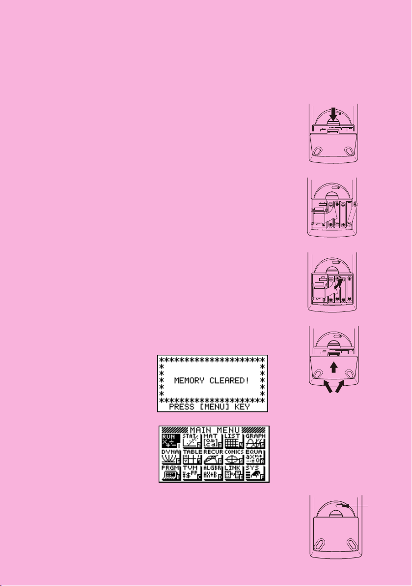
1. Slide the back cover from the unit by pulling with your finger at the point marked 1.

2. Load the four batteries that come with calculator.

• Make sure that the positive (+) and negative (–) ends of the batteries are facing correctly.

MAIMAI

3. Remove the insulating sheet at the location marked “BACK UP” by pulling in the direction indicated by the arrow.

4. Replace the back cover, making sure that its tabs enter the holes marked 2 in the illustration.

5. Press

If the Main Menu shown to the right is not on the display, press the P button on the back of the calculator to perform memory reset.

MAINMAIN

BACK UPBACK UP

6. Use the cursor keys (f, c, d, e) to select the SYS icon and press

w or simply press

7. Use the cursor keys (c, f) to highlight

Color Contrast and then press

the contrast adjustment screen.

8. Adjust the display color.

wto display

uTo adjust the color contrast

1. Use f and c to move the pointer to CONTRAST.

2. Press e to make the figures on the display darker, and d to make them lighter.

uTo adjust the tint

1. Use f and c to move the pointer to the color you want to adjust (ORANGE, BLUE, or GREEN).

2. Press e to add more green to the color, and d to add more orange.

9. To exit display color adjustment, press

REMOVING AND REPLACING THE CALCULATOR'S COVER

To remove the cover

Grasp the top of the cover, and slide the unit out from the bottom.

To replace the cover

Grasp the top of the cover, and slide the unit in from the bottom.

Always slide the unit into the cover with the unit's display end first. Never slide the keyboard end of the unit into the cover.

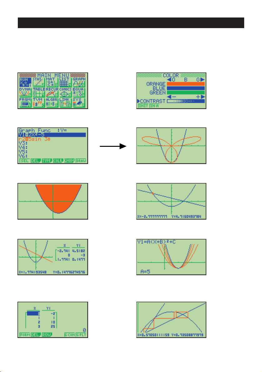
ABOUT THE COLOR DISPLAY

The display uses three colors: orange, blue, and green, to make data easier to understand.

• Main Menu • Display Color Adjustment

• Graph Function Menu

• Graph Display (Example 1) • Graph Display (Example 2)

• Graph-To-Table Display • Dynamic Graph Display

• Table & Graph Numeric Table • Recursion Formula Convergence/ Divergence Graph Example

iii

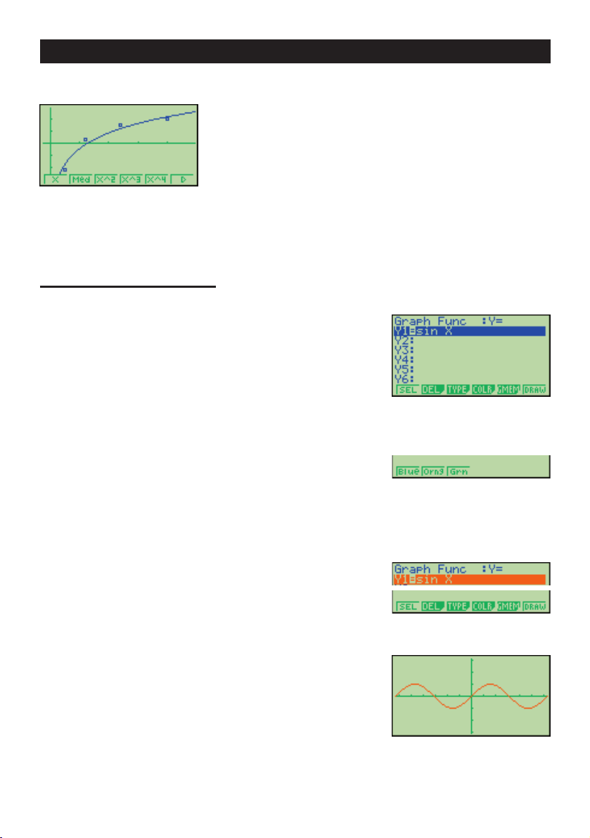
• Statistical Regression Graph Example

• When you draw a graph or run a program, any comment text normally appears on the

display in blue. You can, however, change the color of comment text to orange or green.

Example:

1. Enter the GRAPH Mode and input the following.

To draw a sine curve

3(TYPE)1(Y=)

(Specifies rectangular coordinates.)

svwf

(Stores the expression.)

4(COLR)

• Press the function key that corresponds to the color you want to use for the graph:

3456

1 for blue, 2 for orange, 3 for green.

2(Orng)

(Specifies the graph color.)

4.6(DRAW)

(Draws the graph)

You can also draw multiple graphs of different color on the same screen, making each one distinct and easy to view.

KEYS

Note that pressing / displays the character "/" for division, not "÷".

Alpha Lock

Normally, once you press a and then a key to input an alphabetic character, the keyboard reverts to its primary functions immediately. If you press ! and then a, the keyboard locks in alpha input until you press a again.

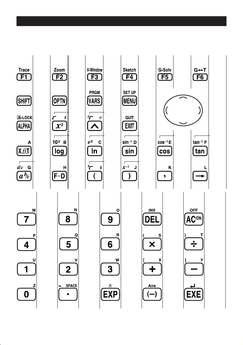
KEY TABLE

Page Page Page Page Page Page

128

2 27 28 3

2 47 46

Page Page Page Page Page

132 113

383 4

47 46

46 46

154 144 120

45 45

Quick-Start

Turning Power On And Off

Auto Power Off Function

Using Modes Basic Calculations

Replay Features

Fraction Calculations Exponents

Graph Functions

Dual Graph

Box Zoom Dynamic Graph

Table Function

Quick-Start

Welcome to the world of color graphing calculators and the CASIO “CFX-9970G”.

Quick-Start is not a complete tutorial, but it takes you through many of the most common functions, from turning the power on, to specifying colors, and on to graphing complex equations. When you’re done, you’ll have mastered the basic operation of the “CFX9970G” and will be ready to proceed with the rest of this user’s guide to learn the entire spectrum of functions available.

Each step of the examples in Quick-Start is shown graphically to help you follow along quickly and easily. When you need to enter the number 57, for example, we’ve indicated it as follows:

Press fh

Whenever necessary, we’ve included samples of what your screen should look like. If you find that your screen doesn’t match the sample, you can restart from the beginning by pressing the “All Clear” button

TURNING POWER ON AND OFF

To turn power on, press o.

To turn power off, press

OFF

AUTO POWER OFF FUNCTION

Note that the unit automatically turns power off if you do not perform any operation for about six minutes (about 60 minutes when a calculation is stopped by an output command (^)).

USING MODES

The “CFX-9970G” makes it easy to perform a wide range of calculations by simply selecting the appropriate mode. Before getting into actual calculations and operation examples, let’s take a look at how to navigate around the modes.

To select the RUN Mode

1. Press m to display the Main Menu.

viii

Quick-Start

2. Use defc to highlight RUN and then

press w.

This is the initial screen of the RUN mode, where you

can perform manual calculations, and run programs.

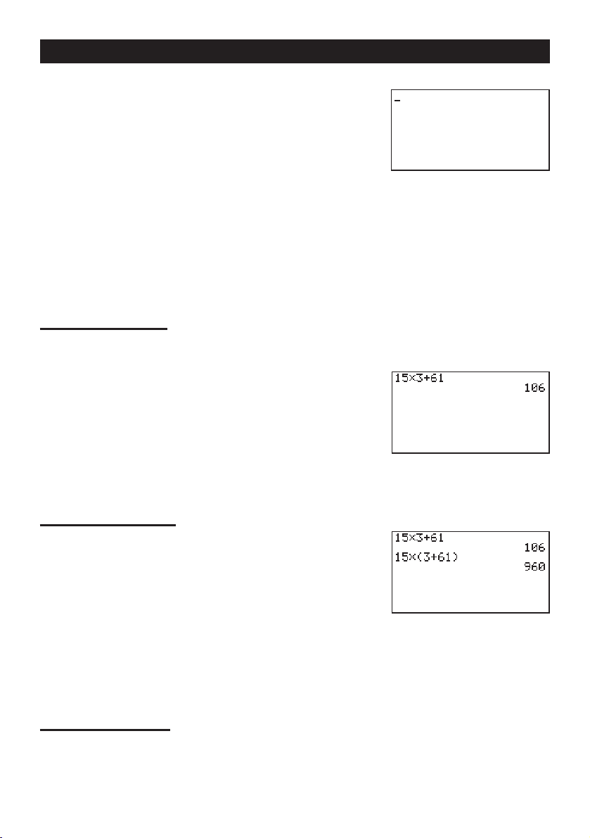
BASIC CALCULATIONS

With manual calculations, you input formulas from left to right, just as they are written on paper. With formulas that include mixed arithmetic operators and parentheses, the calculator automatically applies true algebraic logic to calculate the result.

Example:

1. Press

2. Press

15 ! 3 + 61

o to clear the calculator.

bf*d+gbw.

Parentheses Calculations

Example:

1. Press

15 ! (3 + 61)

bf*(d +gb)w.

Built-In Functions

The “CFX-9970G” includes a number of built-in scientific functions, including trigonometric and logarithmic functions.

Example:

25 ! sin 45˚

Important!

Be sure that you specify Deg (degrees) as the angle unit before you try this example.

1. Press o.

SET UP

2. Press

3. Press cccc1 (Deg) to specify

degrees as the angle unit.

to switch the set up display.

Quick-Start

4. Press

5. Press

6. Press

J to clear the menu.

o to clear the unit.

cf*sefw.

REPLAY FEATURES

With the replay feature, simply press d or e to recall the last calculation that was

performed. This recalls the calculation so you can make changes or re-execute it as it is.

Example:

1. Press

2. Press

3. Press f.

To change the calculation in the last example from (25 ! sin 45˚) to (25 ! sin 55˚)

d to display the last calculation.

d twice to move the cursor under the 4.

4. Press

w to execute the calculation again.

Quick-Start

FRACTION CALCULATIONS

You can use the $ key to input fractions into calculations. The symbol “ { ” is used

to separate the various parts of a fraction.

Example:

1. Press o.

2. Press

1 15/16 + 37/

b$bf$ bg+dh$ jw.

Indicates 6 7/

Converting a Mixed Fraction to an Improper Fraction

While a mixed fraction is shown on the display, press !

improper fraction.

Press

d/c

again to convert back to a mixed fraction.

Converting a Fraction to Its Decimal Equivalent

While a fraction is shown on the display, press M to convert it to its decimal equiva-

lent.

M again to convert back to a fraction.

Press

144

d/c

to convert it to an

EXPONENTS

Quick-Start

Example:

1. Press o.

2. Press

3. Press

4. Press

an exponent.

5. Press

1250 ! 2.06

bcfa*c.ag.

M and the ^ indicator appears on the display.

f. The ^5 on the display indicates that 5 is

xii

Quick-Start

GRAPH FUNCTIONS

The graphing capabilities of this calculator makes it possible to draw complex graphs using either rectangular coordinates (horizontal axis: x ; vertical axis: y) or polar coordinates (angle:

; distance from origin: r).

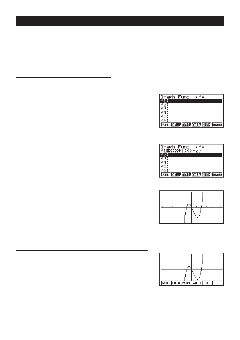
Example

1. Press

2. Use

3. Input the formula.

1: To graph Y = X(X + 1)(X – 2)

d, e, f, and c to highlight GRAPH,

and then press w.

v(v+b)

(v -c)w

4. Press 6 (DRAW) or w to draw the graph.

Example

1. Press

2: To determine the roots of Y = X(X + 1)(X – 2)

! 5 (G-Solv).

xiii

2. Press 1 (ROOT).

Press e for other roots.

Quick-Start

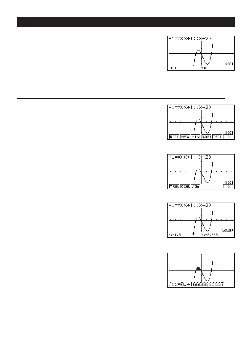
Example

1. Press

2. Press 6 (g).

3. Press

4. Use e to move the pointer to the location where

3: Determine the area bounded by the origin and the X = –1 root obtained for

Y = X(X + 1)(X – 2)

!5 (G-Solv).

3 (#dx).

X = –1, and then press w. Next, use e again

to move the pointer to the location where X = 0, and

then press

becomes shaded on the display.

to input the integration range, which

12345

123456

xiv

Quick-Start

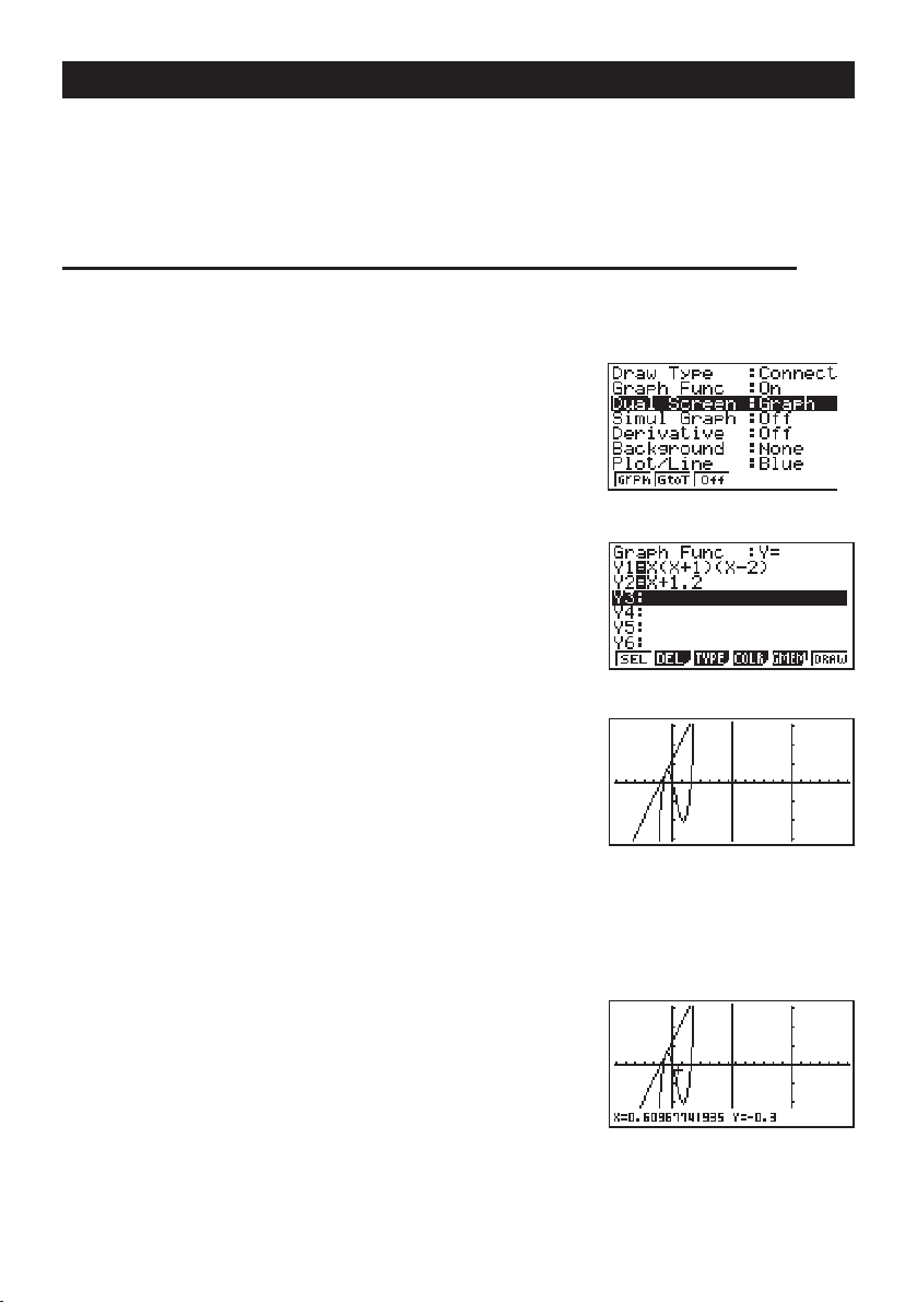
DUAL GRAPH

With this function you can split the display between two areas and display two graphs on the same screen.

Example:

1. Press !Zcc1(Grph) to specify

“Graph” for the Dual Screen setting.

2. Press

To draw the following two graphs and determine the points of intersection

Y1 = X(X + 1)(X – 2) Y2 = X + 1.2

J, and then input the two functions.

v(v+b) (v-c)w v+b.cw

3. Press 6 (DRAW) or w to draw the graphs.

23456

12345

BOX ZOOM

Use the Box Zoom function to specify areas of a graph for enlargement.

1. Press

2. Use

! 2 (Zoom) 1 (BOX).

d, e, f, and c to move the pointer

to one corner of the area you want to specify and then

press

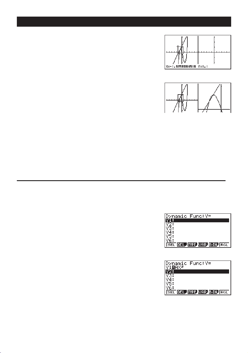
3. Use d, e, f, and c to move the pointer

again. As you do, a box appears on the display. Move

the pointer so the box encloses the area you want to

enlarge.

Quick-Start

4. Press

w, and the enlarged area appears in the

inactive (right side) screen.

DYNAMIC GRAPH

Dynamic Graph lets you see how the shape of a graph is affected as the value assigned to one of the coefficients of its function changes.

Example:

1. Press m.

2. Use

and then press w.

To draw graphs as the value of coefficient A in the following function changes from 1 to 3

Y = AX

d, e, f, and c to highlight DYNA,

3. Input the formula.

aAvxw

12356

xvi

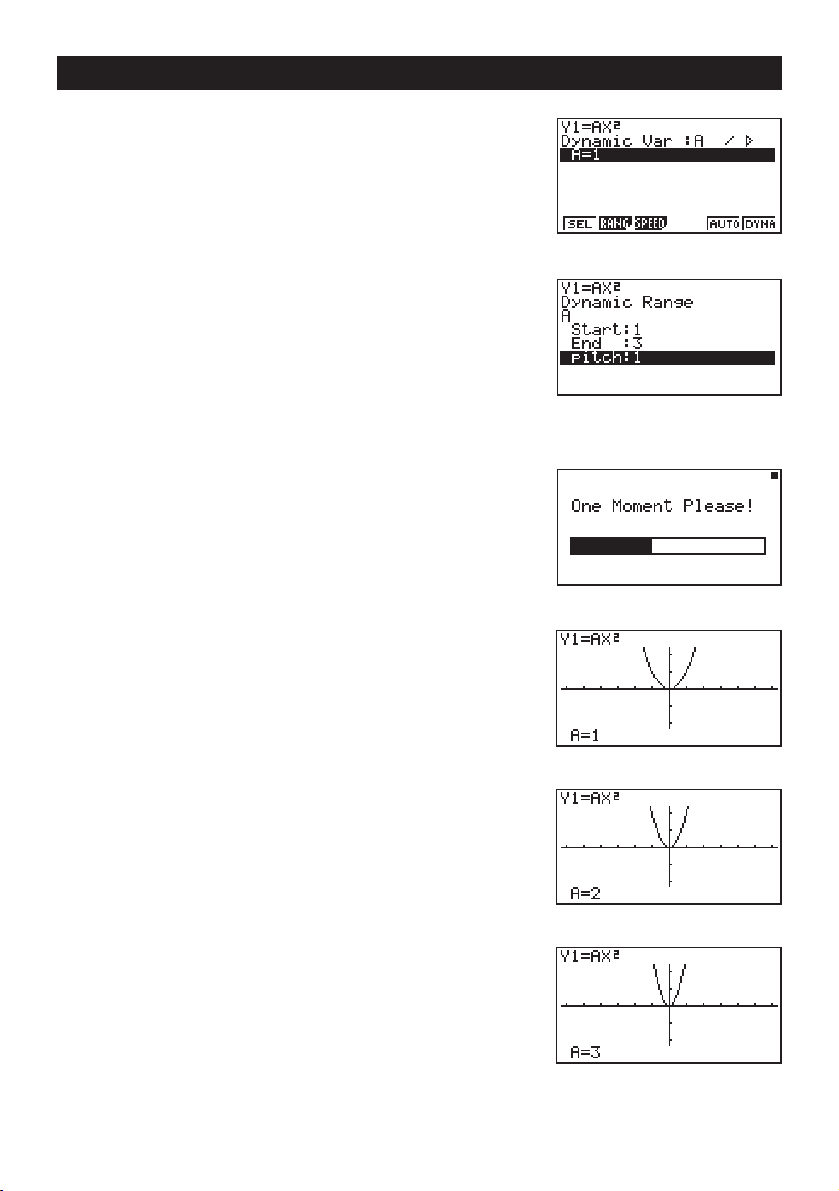
4. Press 4 (VAR) bw to assign an initial value

of 1 to coefficient A.

Quick-Start

5. Press

6. Press

7. Press

2 (RANG) bwdwbw

to specify the range and increment of change in

coefficient A.

6(DYNA) to start Dynamic Graph drawing.

The graphs are drawn 10 times.

3456

xvii

Quick-Start

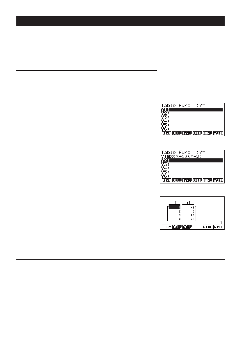
TABLE FUNCTION

The Table Function makes it possible to generate a table of solutions as different values are assigned to the variables of a function.

Example:

1. Press m.

2. Use

and then press w.

3. Input the formula.

To create a number table for the following function

Y = X (X+1) (X–2)

d, e, f, and c to highlight TABLE,

v(v+b)

(v-c) w

4. Press 6 (TABL) or w to generate the number

table.

After you’ve completed this Quick-Start section, you are well on your way to becoming an expert user of the CASIO “CFX-9970G” Calculator.

To learn all about the many powerful features of the “CFX-9970G”, read on and explore!

xviii

Handling Precautions

• Your calculator is made up of precision components. Never try to take it apart.

• Avoid dropping your calculator and subjecting it to strong impact.

• Do not store the calculator or leave it in areas exposed to high temperatures or humidity, or large

amounts of dust. When exposed to low temperatures, the calculator may require more time to display results and may even fail to operate. Correct operation will resume once the calculator is brought back to normal temperature.

• The display will go blank and keys will not operate during calculations. When you are operating the

keyboard, be sure to watch the display to make sure that all your key operations are being performed correctly.

• Replace the main batteries once every 2 years regardless of how much the calculator is used during

that period. Never leave dead batteries in the battery compartment. They can leak and damage the unit.

• Keep batteries out of the reach of small children. If swallowed, consult with a physician immediately.

• Avoid using volatile liquids such as thinner or benzine to clean the unit. Wipe it with a soft, dry cloth,

or with a cloth that has been dipped in a solution of water and a neutral detergent and wrung out.

• Always be gentle when wiping dust off the display to avoid scratching it.

• In no event will the manufacturer and its suppliers be liable to you or any other person for any

damages, expenses, lost profits, lost savings or any other damages arising out of loss of data and/or formulas arising out of malfunction, repairs, or battery replacement. The user should prepare physical records of data to protect against such data loss.

• Never dispose of batteries, the liquid crystal panel, or other components by burning them.

• When the “Low battery!” message appears on the display, replace the main power supply batteries

as soon as possible.

• Be sure that the power switch is set to OFF when replacing batteries.

• If the calculator is exposed to a strong electrostatic charge, its memory contents may be damaged or

the keys may stop working. In such a case, perform the Reset operation to clear the memory and restore normal key operation.

• If the calculator stops operating correctly for some reason, use a thin, pointed object to press the P

button on the back of the calculator. Note, however, that this clears all the data in calculator memory.

• Note that strong vibration or impact during program execution can cause execution to stop or can

damage the calculator’s memory contents.

• Using the calculator near a television or radio can cause interference with TV or radio reception.

• Before assuming malfunction of the unit, be sure to carefully reread this user ’s guide and ensure that

the problem is not due to insufficient battery power, programming or operational errors.

xix

Be sure to keep physical records of all important data!

The large memory capacity of the unit makes it possible to store large amounts of data. You should note, however, that low battery power or incorrect replacement of the batteries that power the unit can cause the data stored in memory to be corrupted or even lost entirely. Stored data can also be affected by strong electrostatic charge or strong impact.

Since this calculator employs unused memory as a work area when performing its internal calculations, an error may occur when there is not enough memory available to perform calculations. To avoid such problems, it is a good idea to leave 1 or 2 kbytes of memory free (unused) at all times.

In no event shall CASIO Computer Co., Ltd. be liable to anyone for special, collateral, incidental, or consequential damages in connection with or arising out of the purchase or use of these materials. Moreover, CASIO Computer Co., Ltd. shall not be liable for any claim of any kind whatsoever against the use of these materials by any other party.

• The contents of this user’s guide are subject to change without notice.

• No part of this user’s guide may be reproduced in any form without the express written consent of the manufacturer.

• The options described in Chapter 22 of this user’s guide may not be available in certain geographic areas. For full details on availability in your area, contact your nearest CASIO dealer or distributor.

• • • • • • • • • • • • • • • • • • •

CFX-9970G

• • • • • • • • • • • • • • • • • • •

Contents

Getting Acquainted — Read This First! ............................................................. 1

1. Key Markings ....................................................................................................... 2

2. Selecting Icons and Entering Modes.................................................................... 3

3. Display ................................................................................................................. 8

4. Color Adjustment................................................................................................ 11

5. When you keep having problems… ................................................................... 12

Chapter 1 Basic Operation ............................................................................. 13

1-1 Before Starting Calculations... ..................................................................... 14

1-2 Memory ....................................................................................................... 22

1-3 Option (OPTN) Menu .................................................................................. 27

1-4 Variable Data (VARS) Menu ........................................................................ 28

1-5 Program (PRGM) Menu .............................................................................. 34

Chapter 2 Manual Calculations ...................................................................... 35

2-1 Basic Calculations ....................................................................................... 36

2-2 Special Functions ........................................................................................ 39

2-3 Function Calculations .................................................................................. 43

Chapter 3 Numerical Calculations ................................................................. 53

3-1 Before Performing a Calculation ................................................................. 54

3-2 Differential Calculations............................................................................... 55

3-3 Quadratic Differential Calculations .............................................................. 58

3-4 Integration Calculations ............................................................................... 60

3-5 Maximum/Minimum Value Calculations ....................................................... 63

3-6 & Calculations.............................................................................................. 65

Chapter 4 Complex Numbers ......................................................................... 67

4-1 Before Beginning a Complex Number Calculation ...................................... 68

4-2 Performing Complex Number Calculations ................................................. 69

Chapter 5 Binary, Octal, Decimal, and Hexadecimal Calculations ............. 73

5-1 Before Beginning a Binary, Octal, Decimal, or Hexadecimal

Calculation ............................................................................................. 74

5-2 Selecting a Number System ........................................................................ 76

5-3 Arithmetic Operations .................................................................................. 77

5-4 Negative Values and Logical Operations .................................................... 78

Chapter 6 Matrix Calculations........................................................................ 79

6-1 Before Performing Matrix Calculations ........................................................ 80

6-2 Matrix Cell Operations ................................................................................. 83

6-3 Modifying Matrices Using Matrix Commands .............................................. 88

6-4 Matrix Calculations ...................................................................................... 92

xxii

Contents

Chapter 7 Equation Calculations ................................................................... 99

7-1 Before Beginning an Equation Calculation ................................................ 100

7-2 Linear Equations with Two to Six Unknowns ............................................. 101

7-3 Quadratic and Cubic Equations................................................................. 104

7-4 Solve Calculations ..................................................................................... 107

7-5 What to Do When an Error Occurs............................................................ 110

Chapter 8 Graphing ....................................................................................... 111

8-1 Before Trying to Draw a Graph .................................................................. 112

8-2 View Window (V-Window) Settings ........................................................... 113

8-3 Graph Function Operations ....................................................................... 117

8-4 Graph Memory .......................................................................................... 122

8-5 Drawing Graphs Manually ......................................................................... 123

8-6 Other Graphing Functions ......................................................................... 128

8-7 Picture Memory ......................................................................................... 139

8-8 Graph Background .................................................................................... 140

Chapter 9 Graph Solve.................................................................................. 143

9-1 Before Using Graph Solve......................................................................... 144

9-2 Analyzing a Function Graph ...................................................................... 145

Chapter 10 Sketch Function ...........................................................................153

10-1 Before Using the Sketch Function ............................................................. 154

10-2 Graphing with the Sketch Function ........................................................... 155

Chapter 11 Dual Graph ................................................................................... 167

11-1 Before Using Dual Graph .......................................................................... 168

11-2 Specifying the Left and Right View Window Parameters .......................... 169

11-3 Drawing a Graph in the Active Screen ...................................................... 170

11-4 Displaying a Graph in the Inactive Screen ................................................ 171

Chapter 12 Graph-to-Table ............................................................................. 175

12-1 Before Using Graph-to-Table..................................................................... 176

12-2 Using Graph-to-Table ................................................................................ 177

Chapter 13 Dynamic Graph ............................................................................ 181

13-1 Before Using Dynamic Graph .................................................................... 182

13-2 Storing, Editing, and Selecting Dynamic Graph Functions ........................ 183

13-3 Drawing a Dynamic Graph ........................................................................ 184

13-4 Using Dynamic Graph Memory ................................................................. 190

13-5 Dynamic Graph Application Examples ...................................................... 191

Chapter 14 Implicit Function Graphs ............................................................ 193

14-1 Before Graphing an Implicit Function ........................................................ 194

14-2 Graphing an Implicit Function .................................................................... 195

14-3 Implicit Function Graph Analysis ............................................................... 199

xxiii

Contents

Chapter 15 Table & Graph .............................................................................. 205

15-1 Before Using Table & Graph ...................................................................... 206

15-2 Storing a Function and Generating a Numeric Table ................................ 207

15-3 Editing and Deleting Functions .................................................................. 210

15-4 Editing Tables and Drawing Graphs .......................................................... 211

15-5 Copying a Table Column to a List .............................................................. 216

Chapter 16 Recursion Table and Graph ........................................................217

16-1 Before Using the Recursion Table and Graph Function ............................ 218

16-2 Inputting a Recursion Formula and Generating a Table ............................ 219

16-3 Editing Tables and Drawing Graphs .......................................................... 223

Chapter 17 List Function ................................................................................ 229

List Data Linking ................................................................................................... 230

17-1 List Operations .......................................................................................... 231

17-2 Editing and Rearranging Lists ................................................................... 233

17-3 Manipulating List Data ............................................................................... 237

17-4 Arithmetic Calculations Using Lists ........................................................... 244

17-5 Switching Between List Files ..................................................................... 248

Chapter 18 Statistical Graphs and Calculations .......................................... 249

18-1 Before Performing Statistical Calculations ................................................ 250

18-2 Paired-Variable Statistical Calculation Examples ...................................... 251

18-3 Calculating and Graphing Single-Variable Statistical Data ........................ 257

18-4 Calculating and Graphing Paired-Variable Statistical Data ....................... 261

18-5 Performing Statistical Calculations ............................................................ 269

18-6 Tests .......................................................................................................... 275

18-7 Confidence Interval ................................................................................... 293

18-8 Distribution ................................................................................................ 303

Chapter 19 Financial Calculations .................................................................319

19-1 Before Performing Financial Calculations ................................................. 320

19-2 Simple Interest Calculations ...................................................................... 322

19-3 Compound Interest Calculations ............................................................... 324

19-4 Investment Appraisal ................................................................................. 335

19-5 Amortization of a Loan .............................................................................. 339

19-6 Conversion between Percentage Interest Rate and Effective

Interest Rate ........................................................................................ 343

19-7 Cost, Selling Price, Margin Calculations ................................................... 345

19-8 Day/Date Calculations ............................................................................... 347

xxiv

Contents

Chapter 20 Algebraic Expressions ................................................................ 349

20-1 Before Using the Algebraic Mode .............................................................. 350

20-2 Inputting and Executing Calculations ........................................................ 351

20-3 ALGBR Mode Commands ......................................................................... 352

20-4 Signum Function ....................................................................................... 360

20-5 Natural Display Notation ............................................................................ 361

20-6 ALGBR Mode Error Messages .................................................................. 362

20-7 ALGBR Mode Precautions ........................................................................ 363

Chapter 21 Programming ............................................................................... 365

21-1 Before Programming ................................................................................. 366

21-2 Programming Examples ............................................................................ 367

21-3 Debugging a Program ............................................................................... 372

21-4 Calculating the Number of Bytes Used by a Program ............................... 373

21-5 Secret Function ......................................................................................... 374

21-6 Searching for a File ................................................................................... 376

21-7 Searching for Data Inside a Program ........................................................ 378

21-8 Editing File Names and Program Contents ............................................... 379

21-9 Deleting a Program ................................................................................... 382

21-10 Useful Program Commands ...................................................................... 383

21-11 Command Reference ................................................................................ 385

21-12 Text Display ............................................................................................... 402

21-13 Using Calculator Functions in Programs ................................................... 403

Chapter 22 Data Communications .................................................................413

22-1 Connecting Two Units ............................................................................... 414

22-2 Connecting the Unit with a Personal Computer ........................................ 415

22-3 Connecting the Unit with a CASIO Label Printer ....................................... 416

22-4 Before Performing a Data Communication Operation ............................... 417

22-5 Performing a Data Transfer Operation ...................................................... 418

22-6 Screen Send Function ............................................................................... 422

22-7 Data Communications Precautions ........................................................... 423

Chapter 23 Program Library ...........................................................................425

1. Prime Factor Analysis ...................................................................................... 426

2. Greatest Common Measure ............................................................................. 428

3. t-Test Value ...................................................................................................... 430

4. Circle and Tangents ......................................................................................... 432

5. Rotating a Figure .............................................................................................. 439

xxv

Contents

Appendix ........................................................................................................... 443

Appendix A Resetting the Calculator ................................................................. 444

Appendix B Power Supply ................................................................................. 446

Appendix C Error Message Table ...................................................................... 450

Appendix D Input Ranges.................................................................................. 453

Appendix E Specifications ................................................................................. 456

Index ..................................................................................................................... 458

Command Index ................................................................................................... 464

Key Index .............................................................................................................. 465

Program Mode Command List .............................................................................. 468

Algebraic Mode Command List............................................................................. 471

xxvi

Getting Acquainted

— Read This First!

About this User’s Guide

uFunction Keys and Menus

• Many of the operations performed by this calculator can be executed by pressing function keys 1 through 6. The operation assigned to each function key changes according to the mode the calculator is in, and current operation assignments are indicated by function menus that appear at the bottom of the display.

• This user’s guide indicates the current operation assigned to a function key in parentheses following the key cap marking for that key. 1 (Comp), for example, indicates that pressing 1 selects {Comp}, which is also indicated in the function menu.

• When {g} is indicated in the function menu for key 6, it means that pressing 6 displays the next page or previous page of menu options.

uMenu Titles

• Menu titles in this user’s guide include the key operation required to display the menu being explained. The key operation for a menu that is displayed by pressing K and then {COLR} would be shown as: [OPTN]-[COLR].

• 6 (g) key operations to change to another menu page are not shown in menu title key operations.

Getting Acquainted — Read This First!

uCommand List

• The Program Mode Command List (page 468) provides a graphic flowchart of the various function key menus that shows how to maneuver to the menu of commands you need.

Example: The following operation displays Xfct: [VARS]-[FACT]-[Xfct]

uIcons Used in This User’s Guide

• The following are the meanings of the icons used in this user’s guide.

: Important : Note : Reference page

P.000

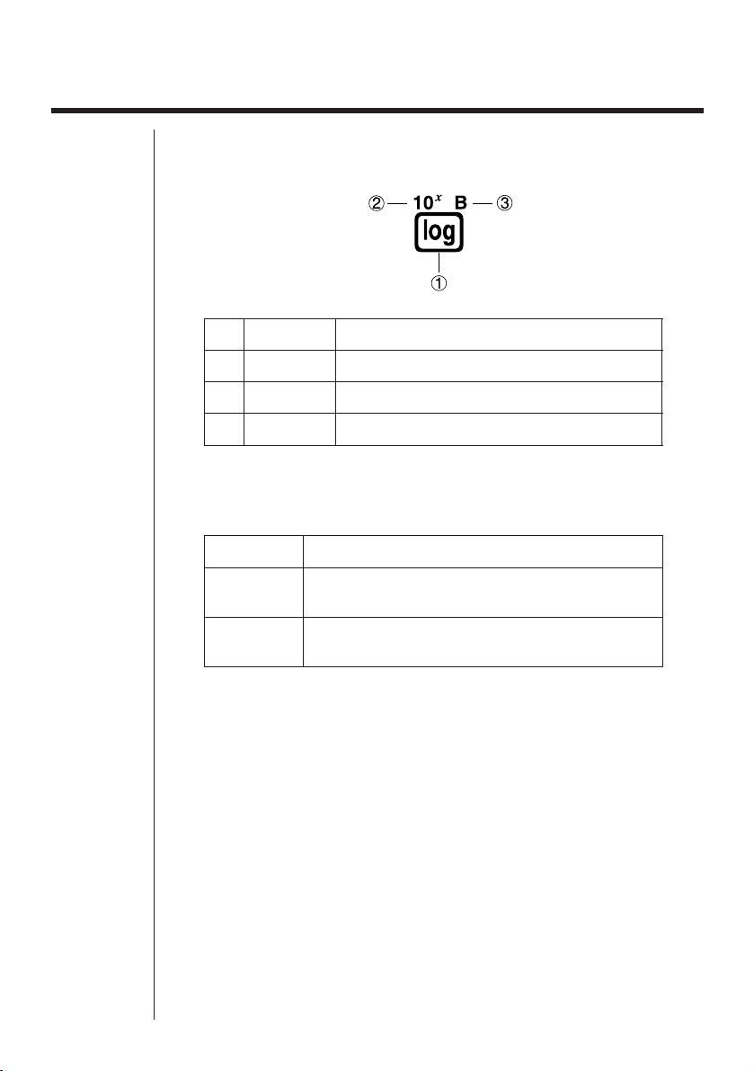
1. Key Markings

Many of the calculator’s keys are used to perform more than one function. The functions marked on the keyboard are color coded to help you find the one you need quickly and easily.

1 log l

2 10

3 B al

The following describes the color coding used for key markings.

Color Key Operation

Orange Press ! and then the key to perform the marked

Function Key Operation

function.

Red Press a and then the key to perform the marked

function.

2. Selecting Icons and Entering Modes

This section describes how to select an icon in the Main Menu to enter the mode you want.

uTo select an icon

1. Press m to display the Main Menu.

Currently selected icon

2. Use the cursor keys (d, e, f, c) to move the highlighting to the icon you want.

3. Press w to display the initial screen of the mode whose icon you selected.

• You can also enter a mode without highlighting an icon in the Main Menu by inputting the number or letter marked in the lower right corner of the icon.

• Use only the procedures described above to enter a mode. If you use any other procedure, you may end up in a mode that is different than the one you thought you selected.

The following explains the meaning of each icon.

Icon Mode Name Description

RUN Use this mode for arithmetic calculations

and function calculations, and for calculations involving binary, octal, decimal and hexadecimal values.

STATistics Use this mode to perform single-variable

(standard deviation) and paired-variable (regression) statistical calculations, to perform tests, to analyze data and to draw statistical graphs.

MATrix Use this mode for storing and editing

matrices.

LIST Use this mode for storing and editing

numeric data.

GRAPH Use this mode to store graph functions and

to draw graphs using the functions.

DYNAmic graph Use this mode to store graph functions and

to draw multiple versions of a graph by changing the values assigned to the variables in a function.

2 Selecting Icons and Entering Modes

Icon Mode Name Description

TABLE Use this mode to store functions, to

RECURsion Use this mode to store recursion formulas,

CONICS Use this mode to draw graphs of implicit

EQUAtion Use this mode to solve linear equations with

PRoGraM Use this mode to store programs in the

Time Value of Use this mode to perform financial calculaMoney tions and to draw cash flow and other types

ALGeBRa Use this mode to obtain mathematical

LINK Use this mode to transfer memory contents

SYStem Use this mode to check how much memory

generate a numeric table of different solutions as the values assigned to variables in a function change, and to draw graphs.

to generate a numeric table of different solutions as the values assigned to variables in a function change, and to draw graphs.

functions.

two through six unknowns, quadratic equations, and cubic equations.

program area and to run programs.

of graphs.

expression results using natural mathematical display notation.

or back-up data to another unit.

is used and remaining, to delete data from memory, and to initialize (reset) the calculator. It also lets you adjust display contrast.

k Using the Set Up Screen

The mode's set up screen shows the current status of mode settings and lets you make any changes you want. The following procedure shows how to change a set up.

uTo change a mode set up

1. Select the icon you want and press w enter a mode and display its initial screen. Here we will enter the RUN Mode.

2. Press !Z to display the mode’s set up screen.

• This set up screen is just one possible example. Actual set up screen contents will differ according to the mode you are in and that mode’s current settings.

1 2 3 4 5

P.75

Selecting Icons and Entering Modes 2

123 4 5

3. Use the f and c cursor keys to move the highlighting to the item whose setting you want to change.

4. Press the function key (1 to 6) that is marked with the setting you want to make.

5. After you are finished making any changes you want, press J to return to the initial screen of the mode.

k Set Up Screen Function Key Menus

This section details the settings you can make using the function keys in the set up display.

uMode (calculation /binary, octal, decimal, hexadecimal mode)

•{Comp} ... {arithmetic calculation mode}

•{Dec}/{Hex}/{Bin}/{Oct} ... {decimal}/{hexadecimal}/{binary}/{octal}

P.123

P.125

P.126

P.128

P.129 P.177 P.209

P.130

P.14

uFunc Type (graph function type)

•{Y=}/{r=}/{Parm}/{X=c} ... {rectangular coordinate}/{polar coordinate}/ {parametric coordinate}/{X = constant} graph

•{Y>}/{Y<}/{Y }/{Y } ... {y>f( x)}/{y<f( x )}/{y'f (x)}/{y( f(x)} inequality graph

• The v key inputs one of three different variable names. Which variable

name it inputs is determined by the {Func Type} setting you make.

uDraw Type (graph drawing method)

•{Con}/{Plot} ... {connected points}/{unconnected points}

uDerivative (derivative value display)

•{On}/{Off} ... {display on}/{display off} while Graph-to-Table, Table & Graph,

and Trace are being used

uAngle (default unit of angular measurement)

•{Deg}/{Rad}/{Gra} ... {degrees}/{radians}/{grads}

uCoord (graph pointer coordinate display)

•{On}/{Off} ... {display on}/{display off}

2 Selecting Icons and Entering Modes

uGrid (graph gridline display)

P.121

P.14 P.15

P.60

P.251

•{On}/{Off} ... {display on}/{display off}

uAxes (graph axis display)

•{On}/{Off} ... {display on}/{display off}

uLabel (graph axis label display)

•{On}/{Off} ... {display on}/{display off}

uDisplay (display format)

•{Fix}/{Sci}/{Norm}/{Eng} ... {fixed number of decimal places specification}/ {number of significant digits specification}/{exponential format display range toggle}/{Engineering Mode}

uIntegration (Integration calculation)

•{Gaus}/{Simp} ... integration calculation using {Gauss-Kronrod rule}/ {Simpson’s rule}.

uStat Wind (statistical graph view window setting method)

•{Auto}/{Man} ... {automatic}/{manual}

P.187

P.140

P.266

P.248

uGraph Func (function display during graph drawing and trace)

•{On}/{Off} ... {display on}/{display off}

uBackground (graph display background)

•{None}/{PICT} ... {no background}/{graph background picture specification}

uPlot/Line (plot and line graph color setting)

• {Blue}/{Orng}/{Grn} ... {blue}/{orange}/{green}

uResid List (residual calculation)

•{None}/{LIST} ... {no calculation}/{list specification for the calculated residual data}

uList File (list file specification)

•{File 1} to {File 6} ... {specification of which list file to display while using the List function}

P.168 P.176

P.215

P.186 P.187

P.188

P.208

Selecting Icons and Entering Modes 2

uDual Screen (Dual Screen Mode status)

The Dual Screen Mode settings you can make depends on whether you pressed !Z while in the GRAPH Mode, TABLE Mode, or RECUR Mode.

GRAPH Mode

•{Grph}/{GtoT}/{Off} ... {graphing on both sides of Dual Screen}/{graph on one side and numeric table on the other side of Dual Screen}/{Dual Screen off}

TABLE/RECUR Mode

•{T+G}/{Off} ... {graph on one side and numeric table on the other side of Dual Screen}/{Dual Screen off}

uSimul Graph (simultaneous graphing mode)

•{On}/{Off} ... {simultaneous graphing on (all graphs drawn simultaneously)}/ {simultaneous graphing off (graphs drawn in area numeric sequence)}

uDynamic Type (Dynamic Graph type)

•{Cnt}/{Stop} ... {non-stop (continuous)}/{automatic stop after 10 draws}

uLocus (Dynamic Graph Locus Mode)

•{On}/{Off} ... {locus identified by color}/{locus not drawn}

uVariable (Table Generation and Graph Draw settings)

•{Rang}/{LIST} ... {use table range}/{use list data}

P.224

P.329

P.322

P.362

u& Display (& value display in recursion table)

•{On}/{Off} ... {display on}/{display off}

uSlope (display of derivative at current pointer location in implicit

function graph)

•{On}/{Off} ... {display on}/{display off}

uPayment (payment period setting)

•{BGN}/{END} ... {beginning}/{end} setting of payment period

uDate Mode (number of days per year setting)

•{365}/{360} ... interest calculations using {365}/{360} days per year

* The 365-day year must be used for date calculations in the Financial Mode.

Otherwise, an error occurs.

uAnswer Type (type of numbers for results)

• {Real}/{Cplx} ... {use real numbers only}/{include imaginary numbers} when displaying results of processes with real number expressions.

2 Selecting Icons and Entering Modes

3. Display

k About the Display Screen

This calculator uses two types of display: a text display and a graphic display. The text display can show 21 columns and eight lines of characters, with the bottom line used for the function key menu, while the graph display uses an area that measures 127 (W) ! 63 (H) dots.

Text Display Graph Display

k About Display Colors [OPTN]-[COLR]

The calculator can display data in three colors: orange, blue, and green. The default color for graphs and comment text is blue, but you can specify orange or green if you want.

•{Orng}/{Grn} ... {orange}/{green}

• The above setting affects the color of graphs and comment text. Specify the

color you want to use before inputting the graph’s function or the program comment text.

k About Menu Item Types

This calculator uses certain conventions to indicate the type of result you can expect when you press a function key.

• Next Menu

Example:

Selecting displays a menu of hyperbolic functions.

• Command Input

Example:

Selecting inputs the sinh command.

Display 3

• Direct Command Execution

Example: Selecting executes the DRAW command.

k Exponential Display

The calculator normally displays values up to 10 digits long. Values that exceed this limit are automatically converted to and displayed in exponential format. You can specify one of two different ranges for automatic changeover to exponential display.

Norm 1 ........... 10–2 (0.01) > |x|, |x| > 10

Norm 2 ........... 10–9 (0.000000001) > |x|, |x| > 10

uTo change the exponential display range

1. Press !Z to display the set up screen.

2. Use f and c to move the highlighting to “Display”.

3. Press 3 (Norm).

The exponential display range switches between Norm 1 and Norm 2 each time you perform the above operation. There is no display indicator to show you which exponential display range is currently in effect, but you can always check it by seeing what results the following calculation produces.

Ab/caaw

(Norm 1)

(Norm 2)

All of the examples in this manual show calculation results using Norm 1.

uHow to interpret exponential format

1.2E+12 indicates that the result is equivalent to 1.2 ! 1012. This means that you should move the decimal point in 1.2 twelve places to the right, because the exponent is positive. This results in the value 1,200,000,000,000.

1.2E–03 indicates that the result is equivalent to 1.2 ! 10–3. This means that you should move the decimal point in 1.2 three places to the left, because the exponent is negative. This results in the value 0.0012.

3 Display

k Special Display Formats

This calculator uses special display formats to indicate fractions, hexadecimal values, and sexagesimal values.

uFractions

..... Indicates: 456

––––

uHexadecimal Values

..... Indicates: ABCDEF12(16), which

equals –1412567278(10)

uSexagesimal Values

..... Indicates: 12° 34’ 56.78"

• In addition to the above, this calculator also uses other indicators or symbols,

which are described in each applicable section of this manual as they come up.

k Calculation Execution Indicator

Whenever the calculator is busy drawing a graph or executing a long, complex calculation or program, a black box (k) flashes in the upper right corner of the display. This black box tells you that the calculator is performing an internal operation.

4. Color Adjustment

Adjust the color whenever objects on the display appear dim or difficult to see. There are two different settings you can make to get color the way you want it.

• Color contrast

• Tint adjustment for each color

uTo display the color adjustment screen

1. Highlight the SYS icon in the Main Menu and then press w.

2. Highlight Color Contrast and then press w.

•{INIT}/{IN·A} ... {initialize highlighted color}/

{initialize all colors}

Use the following procedures while the color adjustment screen is on the display to adjust the color contrast and tint settings.

uTo adjust the color contrast

1. Use the cursor f and c keys to move the pointer so it is next to CONTRAST.

2. Press the e cursor key to make the display darker and the d cursor key to make it lighter. Holding down either key changes the setting at high speed.

uTo adjust the color tint

1. Use the cursor f and c keys to move the pointer so it is next to the color (ORANGE, BLUE, GREEN) whose tint you want to adjust.

2. Press the e cursor key to give the color a greener tint and the d cursor key to give it an orange tint. Holding down either key changes the setting at high speed.

uTo exit the color adjustment screen

Press m to return to the Main Menu.

• It is recommended that you always adjust the CONTRAST setting first, and then adjust the tint settings for individual colors.

• You can change the CONTRAST setting at any time without displaying the color adjustment screen. Simply press ! and then d or e to change the setting. Press ! once again after get the display looking the way you want.

5. When you keep having problems…

If you keep having problems when you are trying to perform operations, try the following before assuming that there is something wrong with the calculator.

k Get the Calculator Back to its Original Mode Settings

1. In the Main Menu, select the RUN icon and press w.

2. Press ! Z to display the set up screen.

3. Highlight “Angle” and press 2 (Rad).

4. Highlight “Display” and press 3 (Norm) to select the exponential display range (Norm 1 or Norm 2) that you want to use.

P.3

P.445

5. Now enter the correct mode and perform your calculation again, monitoring the results on the display.

k In Case of Hang Up

• Should the unit hang up and stop responding to input from the keyboard, press the P button on the back of the calculator to reset the memory. Note, however, that this clears all the data in calculator memory.

k Low Battery Message

The low battery message appears whenever you press o to turn power on or m to display the Main Menu while the main battery power is below a certain

level.

P.447

o or m

About 3 seconds later

If you continue using the calculator without replacing batteries, power will automatically turn off to protect memory contents. Once this happens, you will not be able to turn power back on, and there is the danger that memory contents will be corrupted or lost entirely.

• You will not be able to perform data communications operations once the low battery message appears.

Chapter

Basic Operation

1-1 Before Starting Calculations...

1-2 Memory

1-3 Option (OPTN) Menu 1-4 Variable Data (VARS) Menu

1-5 Program (PRGM) Menu

1-1 Before Starting Calculations...

Before performing a calculation for the first time, you should use the set up screen to specify the angle unit and display format.

k Setting the Angle Unit (Angle)

1. Display the set up screen and use the f and c keys to highlight “Angle”.

2. Press the function key for the angle unit you want to specify.

•{Deg}/{Rad}/{Gra} ... {degrees}/{radians}/{grads}

3. Press J to return to the screen that was on the display when you started the

procedure.

• The relationship between degrees, grads, and radians is shown below.

360° = 2! radians = 400 grads

90° = !/2 radians = 100 grads

k Setting the Display Format (Display)

1. Display the set up screen and use the f and c keys to highlight “Display”.

2. Press the function key for the item you want to set.

•{Fix}/{Sci}/{Norm}/{Eng} ... {fixed number of decimal places specification}/

{number of significant digits specification}/{exponential format display range toggle}/{Engineering Mode}

3. Press J to return to the screen that was on the display when you started the

procedure.

u To specify the number of decimal places (Fix)

Example To specify two decimal places

1 (Fix) 3 (2)

Press the function key that corresponds to the number of decimal places you want to specify

= 0 to 9).

(

• Displayed values are rounded off to the number of decimal places you specify.

Before Starting Calculations... 1 - 1

u To specify the number of significant digits (Sci)

Example To specify three significant digits

2 (Sci) 4 (3)

Press the function key that corresponds to the number of significant digits you want to

specify (

= 0 to 9).

• Displayed values are rounded off to the number of significant digits you specify.

• Specifying 0 makes the number of significant digits 10.

u To specify the exponential display range (Norm 1/Norm 2)

Press 3 (Norm) to switch between Norm 1 and Norm 2.

Norm 1: 10

Norm 2: 10

u To specify the engineering notation display (Eng)

–2

(0.01)>|x|, |x| >10

–9

(0.000000001)>|x|, |x| >10

Press 4 (Eng) to switch between engineering notation and standard notation. The indicator “/E” is on the display while engineering notation is in effect.

The following are the 11 engineering notation symbols used by this calculator.

Symbol Meaning Unit

E Exa 10

P Peta 10

T Tera 10

G Giga 10

M Mega 10

k kilo 10

Symbol Meaning Unit

m milli 10

µ micro 10

n nano 10

p pico 10

f femto 10

• The engineering symbol that makes the mantissa a value from 1 to 1000 is automatically selected by the calculator when engineering notation is in effect.

–3

–6

–9

–12

–15

1 - 1 Before Starting Calculations...

k Inputting Calculations

When you are ready to input a calculation, first press A to clear the display. Next, input your calculation formulas exactly as they are written, from left to right, and press w to obtain the result.

Example 1 2 + 3 – 4 + 10 =

Ac+d-e+baw

Example 2 2(5 + 4) ÷ (23 " 5) =

Ac(f+e)/

(cd*f)w

k Calculation Priority Sequence

This calculator employs true algebraic logic to calculate the parts of a formula in the following order:

1 Coordinate transformation Pol (x, y), Rec (r, #)

Differentials, quadratic differentials, integrations, $ calculations

d/dx, d

/dx2, %dx, $, Mat, Solve, FMin, FMax, List!Mat, Fill, Seq, SortA, SortD,

Min, Max, Median, Mean, Augment, Mat!List, List

ALGBR Mode unique commands

expand(, factor(, tExpand(, tCollect(, % (, diff(, solve(, tanLine(, collect(, combine(, sequence(, sumSeq(, expToTrig(, trigToExp(, signum(

2 Type A functions

With these functions, the value is entered and then the function key is pressed.

, x–1, x !, ° ’ ”, ENG symbols

3 Power/root ^(xy), 4 Fractions a

5 Abbreviated multiplication format in front of !, memory name, or variable name.

2!, 5A, X min, F Start, etc.

6 Type B functions

With these functions, the function key is pressed and then the value is entered.

, 3, log, In, ex, 10x, sin, cos, tan, sin–1, cos–1, tan–1, sinh, cosh, tanh, sinh–1,

cosh–1, tanh–1, (–), d, h, b, o, Neg, Not, Det, Trn, Dim, Identity, Sum, Prod, Cuml, Percent, AList

7 Abbreviated multiplication format in front of Type B functions

, A log2, etc.3

8 Permutation, combination nPr, nCr

9 " , / (÷) 0 +, –

Before Starting Calculations... 1 - 1

! Relational operator

=, G, >, <, &, '

@ And, and

# Or, or, xor, xnor

• Execution is normally performed from left to right, except in the following cases when it is performed from right to left.

·When functions with the same priority are used in series:

In ( ex{In( )}

120 120

·When power calculations are used in series in the ALGBR Mode:

[5^3^2 ( 5^(3^2)]

·To produce the same result in the RUN Mode, the above calculation should be input: (5^3)^2

• Compound functions are executed from right to left.

• Anything contained within parentheses receives highest priority.

Example 2 + 3 " (log sin2!2 + 6.8) = 22.07101691 (angle unit = Rad)

k Multiplication Operations without a Multiplication Sign

You can omit the multiplication sign (") in any of the following operations.

Example 2sin30, 10log1.2, 2 , 2Pol(5, 12), etc.

• Before constants, variable names, memory names

Example 2!, 2AB, 3Ans, 3Y1, etc.

• Before an open parenthesis

Example 3(5 + 6), (A + 1)(B – 1), etc.

1 - 1 Before Starting Calculations...

k Stacks

The unit employs memory blocks, called and commands. There is a 10-level

stack

, and a 10-level calculation so complex that it exceeds the capacity of available numeric value stack or command stack space, or if execution of a program subroutine exceeds the capacity of the subroutine stack.

Example

program subroutine stack

Numeric Value Stack Command Stack

stacks

, for storage of low priority values

numeric value stack

. An error occurs if you perform a

, a 26-level

command

P.16

P.20

...

( (

(

...

• Calculations are performed according to the priority sequence. Once a calculation is executed, it is cleared from the stack.

• Storing a complex number takes up two numeric value stack levels.

• Storing a two-byte function takes up two command stack levels.

k Input, Output and Operation Limitations

The allowable range for both input and output values is 10 digits for the mantissa and 2 digits for the exponent. Internally, however, the unit performs calculations using 15 digits for the mantissa and 2 digits for the exponent.

Example 3 " 105 ÷ 7 – 42857 =

AdEf/hw

dEf/h-

ecifhw

Before Starting Calculations... 1 - 1

k Overflow and Errors

Exceeding a specified input or calculation range, or attempting an illegal input causes an error message to appear on the display. Further operation of the calculator is impossible while an error message is displayed. The following events cause an error message to appear on the display.

P.453

P.7

• When any result, whether intermediate or final, or any value in memory exceeds ±9.999999999 " 10

• When an attempt is made to perform a function calculation that exceeds the input range (Ma ERROR).

• When an illegal operation is attempted during statistical calculations (Ma ERROR). For example, attempting to obtain 1VAR without data input.

• When the capacity of the numeric value stack or command stack is exceeded (Stk ERROR). For example, entering 25 successive ( followed by 2 + 3 * 4 w.

• When an attempt is made to perform a calculation using an illegal formula (Syn ERROR). For example, 5 ** 3 w.

• When you try to perform a calculation that causes memory capacity to be exceeded (Mem ERROR).

• When you use a command that requires an argument, without providing a valid argument (Arg ERROR).

• When an attempt is made to use an illegal dimension during matrix calculations (Dim ERROR).

• When no solution exists for an ALGBR Mode operation (Undefined).

• When the result of an ALGBR Mode operation exceeds the range of the calculator (Overflow ERROR).

• When a value input in the ALGBR Mode is outside the domain of the operation being performed (Domain ERROR).

• When an ALGBR Mode operation in which only real numbers have been input produces a result that is a complex number while the set up screen's Answer Type item is specified as "Real" (Non-Real ERROR).

• When no solution can be obtained using the Solve Function in the ALGBR Mode (No Solution).

• When an attempt is made to use approx with an expression that generates an error unique to the ALGBR Mode (Ma ERROR).

(Ma ERROR).

P.450

P.41

• Other errors can occur during program execution. Most of the calculator’s keys are inoperative while an error message is displayed. You can resume operation using one of the two following procedures.

• Press the A key to clear the error and return to normal operation.

• Press d or e to display the error.

1 - 1 Before Starting Calculations...

k Memory Capacity

Each time you press a key, either one byte or two bytes is used. Some of the functions that require one byte are: b, c, d, sin, cos, tan, log, In, , and !. Some of the functions that take up two bytes are d/dx(, Mat, Xmin, If, For, Return, DrawGraph, SortA(, PxIOn, Sum, and

When the number of bytes remaining drops to five or below, the cursor automatically changes from “ _ ” to “ v ”. If you still need to input more, you should divide your calculation into two or more parts.

• As you input numeric values or commands, they appear flush left on the display. Calculation results, on the other hand, are displayed flush right, except in the ALGBR Mode.

k Graphic Display and Text Display

The unit uses both a graphic display and a text display. The graphic display is used for graphics, while the text display is used for calculations and instructions. The contents of each type of display are stored in independent memory areas.

uTo switch between the graphic display and text display

Press !6(G)T). You should also note that the key operations used to clear each type of display are different.

uTo clear the graphic display

Press !4(Sketch) 1(Cls) w.

an+1.

uTo clear the text display

Press A.

k Editing Calculations

Use the d and e keys to move the cursor to the position you want to change, and then perform one of the operations described below. After you edit the calculation, you can execute it by pressing w, or use e to move to the end of the calculation and input more.

uTo change a step

Example To change cos60 to sin60

cga

ddd

Before Starting Calculations... 1 - 1

uTo delete a step

Example To change 369 " " 2 to 369 " 2

dgj**c

ddD

uTo insert a step

Example To change 2.362 to sin2.36

c.dgx

ddddd

• When you press ![ the insert location is indicated by the symbol ‘‘t’’. The next function or value you input is inserted at the location of ‘‘t’’. To abort the insert operation without inputting anything, move the cursor, press ![ again, or press d, e or w.

1-2 Memory

k Variables

This calculator comes with 28 variables as standard. You can use variables to store values to be used inside of calculations. Variables are identified by singleletter names, which are made up of the 26 letters of the alphabet, plus r and #. The maximum size of values that you can assign to variables is 15 digits for the mantissa and 2 digits for the exponent. Variable contents are retained even when you turn power off.

uTo assign a value to a variable

Example To assign 123 to variable A

Example To add 456 to variable A and store the result in variable B

uTo display the contents of a variable

Example To display the contents of variable A

[value] a [variable name] w

AbcdaaAw

AaA+efgaaBw

AaAw

uTo clear a variable

Example To clear variable A

Aa a aAw

• To clear all variables, select “Memory Usage” from the SYS Mode.

uTo assign the same value to more than one variable

[value]a [first variable name]a3(~) [last variable name]w

r” or “

• You cannot use “

Example To assign a value of 10 to variables A through F

Abaa!aA

3(~)Fw

” as a variable name in the above operation.

Memory 1 - 2

k Function Memory [OPTN]-[FMEM]

Function memory is convenient for temporary storage of often-used expressions. For longer term storage, we recommend that you use the GRAPH Mode for expressions and the PRGM Mode for programs.

P.27

•{STO}/{RCL}/{fn}/{SEE} ... {function store}/{function recall}/{function area

specification as a variable name inside an expression}/{function list}

uTo store a function

Example To store the function (A+B) (A–B) as function memory number 1

K6(g)6(g)3(FMEM)A

(aA+aB)

(aA-aB)

1(STO) 1(f

• If the function memory number you assign a function to already contains a function, the previous function is replaced with the new one.

uTo recall a function

Example To recall the contents of function memory number 1

K6(g)6(g)3(FMEM)A 2(RCL)1(f

• The recalled function appears at the current location of the cursor on the display.

uTo display a list of available functions

K6(g)6(g)3(FMEM) 4(SEE)

1 - 2 Memory

uTo delete a function

Example To delete the contents of function memory number 1

K6(g)6(g)3(FMEM)A 1(STO) 1(f

• Executing the store operation while the display is blank deletes the function in the function memory you specify.

uTo use stored functions

Once you store a function in memory, you can recall it and use it for a calculation. This feature is very useful for quick and easy input of functions when programming or graphing.

P.111

Example To store x3 + 1, x2 + x into function memory, and then graph:

!Zc1(Y=)JK6(g)6(g)3(FMEM)

AvMd+b1(STO)1(f

Avx+v1(STO)2(f2)(stores (x2 + x))

A!4(Sketch)1(Cls)w !4(Sketch)5(GRPH)1(Y=)

K6(g)6(g)3(FMEM)

3(f

• For full details about graphing, see “8. Graphing”.

k Memory Status

You can check how much memory is used for storage for each type of data. You can also see how many bytes of memory are still available for storage.

uTo check the memory status

1. In the Main Menu, select the SYS icon and

press w.

y = x

+ x2 + x + 1

Use the following View Window parameters.

Xmin = –4 Ymin = –10

Xmax = 4 Ymax = 10

Xscale = 1 Yscale = 1

1)(stores (x

n)1(f1)+2(f2)w

+ 1))

Memory 1 - 2

2. Press c w to display the memory status

screen.

Number of bytes still free

3. Use f and c to move the highlighting and view the amount of memory (in

bytes) used for storage of each type of data.

The following table shows all of the data types that appear on the memory status screen.

Data Type Meaning

Program Program data

Statistics Statistical calculations and graphs

Matrix Matrix memory data

List File List data

Y= Graph functions

Draw Memory Graph drawing conditions (View Window,

enlargement/reduction factor, graph screen)

Graph Memory Graph memory data

View Window View Window memory data

Picture Graph screen data

Dynamic Graph Dynamic Graph data

Table Function Table & Graph data

Recursion Recursion Table & Graph data

Equation Equation calculation data

Alpha Memory Alpha memory data

Function Mem Function memory data

Financial Financial data

1 - 2 Memory

k Clearing Memory Contents

Use the following procedure to clear data stored in memory.

1. In the memory status screen, use f and c to move the highlighting to the

data type you want to clear.

If the data type you select in step 1 allows deletion of specific data

2. Press 1 (DEL).

123456

* This menu appears when you

select List File.

3. Press the function key that corresponds to the data you want to delete.

1 23456

• The above example shows the function menu that appears when you highlight {List File} in step 1.

4. Press 1 (YES).

If the data type you select in step 1 allows deletion of all data only

2. Press 1 (DEL).

3. Press 1 (YES) to delete all of the data.

1 23456

1-3 Option (OPTN) Menu

The option menu gives you access to scientific functions and features that are not marked on the calculator’s keyboard. The contents of the option menu differ according to the mode you are in when you press the K key.

See the Command List at the back of this user’s guide for details on the option (OPTN) menu.

uOption Menu in the RUN and PRGM Modes

P.237

P.88

P.68

P.271

P.43

P.44

P.139

P.23

P.51

•{LIST} ... {list function menu}

•{MAT} ... {matrix operation menu}

•{CPLX} ... {complex number calculation menu}

•{CALC} ... {functional analysis menu}

•{STAT} ... {paired-variable statistical estimated value menu}

•{COLR} ... {graph color menu}

•{HYP} ... {hyperbolic calculation menu}

•{PROB} ... {probability/distribution calculation menu}

•{NUM} ... {numeric calculation menu}

•{ANGL} ... {menu for angle/coordinate conversion, sexagesimal input/

conversion}

•{ESYM} ... {engineering symbol menu}

•{PICT} ... {graph save/recall menu}

•{FMEM} ... {function memory menu}

•{LOGIC} ... {logic operator menu}

Pressing K causes the following function key menu to appear while binary, octal, decimal, or hexadecimal is set as the default number system.

•{COLR} ... {graph color menu}

uOption Menu during numeric data input in the STAT, MAT, LIST,

TABLE, RECUR and EQUA Modes

•{LIST}/{HYP}/{PROB}/{NUM}/{ANGL}/{ESYM}/{FMEM}/{LOGIC}

uOption Menu during formula input in the GRAPH, DYNA, TABLE,

RECUR and EQUA Modes

•{List}/{CALC}/{HYP}/{PROB}/{NUM}/{FMEM}/{LOGIC}

uOption Menu during expression input in the ALGBR Mode

•{Abs}/{HYP}/{ i }/{x!}/{sign}/{FMEM}

The meanings of the option menu items are described in the sections that cover each mode.

1-4 Variable Data (VARS) Menu

To recall variable data, press J to display the variable data menu.

{V-WIN}/{FACT}/{STAT}/{GRPH}/{DYNA}/{TABL}/{RECR}/{EQUA}/{TVM}

See the Command List at the back of this user’s guide for details on the variable data (VARS) menu.

• Note that the EQUA and TVM items appear for function keys (3 and 4) only when you access the variable data menu from the RUN or PRGM Mode.

• The variable data menu does not appear if you press J while binary, octal, decimal, or hexadecimal is set as the default number system.

k V-WIN — Recalling View Window values

P.113

P.134

Selecting {V-WIN} from the VARS menu displays the View Window value recall menu.

u {X}/{Y}/{T,# } ... {x-axis menu}/{y-axis menu}/{T,

u {R-X}/{R-Y}/{R-T,# } ... {x-axis menu}/{y-axis menu}/{T,

of Dual Graph

The following are the items that appear in the above menus.

• {min}/{max}/{scal}/{ptch} ... {minimum value}/{maximum value}/{scale}/

{pitch}

k FACT — Recalling enlargement/reduction factors

Selecting {FACT} from the VARS menu displays the enlargement/reduction factor recall menu.

• {Xfct}/{Yfct} ... {x-axis factor}/{y-axis factor}

menu}

menu} for right side

P.259 P.267

k STAT — Recalling Single/Paired-variable Statistical Data

Selecting {STAT} from the VARS menu displays the single/paired-variable statistical data recall menu.

{X}/{Y}/{GRPH}/{PTS}/{TEST}/{RESLT}

u {X}/{Y} ... {x-data menu}/{y-data menu}

The following are the items that appear in the above menus.

•{n} ... {number of data}

•{

o}/{

p} ... mean of {

•{$x}/{$y} ... sum of {x-data}/{y-data}

}/{$y2} ... sum of squares of {x-data}/{y-data}

•{$

xy} ... {sum of products of x-data and y-data}

•{$

x-data}/{y-data}

Variable Data (VARS) Menu 1 - 4

x*n}/{y*n} ... population standard deviation of {x-data}/{y-data}

•{

•{x*n-1}/{y*n-1} ... sample standard deviation of {x-data}/{y-data}

•{minX}/{minY} ... minimum value of {x-data}/{y-data}

•{maxX}/{maxY} ... maximum value of {

u {GRPH} ...{graph data menu}

The following are the items that appear in the above menu.

•{a}/{b}/{c}/{d}/{e} ... {regression coefficient and multinomial coefficients}

•{r} ... {correlation coefficient}

•{Q1}/{Q3} ... {first quartile}/{third quartile}

•{Med}/{Mod} ... {median}/{mode} of input data

•{Strt}/{Pitch} ... histogram {start division}/{pitch}

•{Iter}/{Perid} ... sine regression {number of iterations}/{period}

u {PTS} ... {summary point data menu}

The following are the items that appear in the above menu.

• {x1}/{y1}/{x2}/{y2}/{x3}/{y3} ... {coordinates of summary points}

u {TEST} ... {test data recall}

The following are the items that appear in the above menu.

• {

n}/{

o}/{x*n-1} ... {number of data}/{data mean}/{sample standard deviation}

• {n1}/{n2} ... number of {data 1}/{data 2}

• {

o1}/{

o2} ... mean of {data 1}/{data 2}

• {x1*}/{x2*} ... sample standard deviation of {data 1}/{data 2}

• {xp*} ... {pooled sample standard deviation}

• {

F} ... {F value}

• {Fdf}/{SS}/{MS} ... factor {degrees of freedom}/{sum of squares}/{mean of

squares}

• {Edf}/{SSe}/{MSe} ... error {degrees of freedom}/{sum of squares}/{mean of

squares}

x-data}/{y-data}

u {RESLT} ... {test result recall}

The following are the items that appear in the above menu.

p} ... {p value}

• {

• {z}/{t}/{Chi}/{F} ... {Z test results}/{t test results}/{+2 test results}/{F test

results}

• {Left}/{Right} ... {interval lower limit (left edge)}/{interval upper limit (right

edge)}

• {

ˆp }/{ˆp 1}/{ˆp 2} ... {expected probability value}/{expected probability value 1}/

{expected probability value 2}

• {df}/{s}/{r}/{r2} ... {degrees of freedom}/{standard error}/{correlation

coefficient}/{coefficient of determination}

1 - 4 Variable Data (VARS) Menu

k GRPH — Recalling Graph Functions

Selecting {GRPH} from the VARS menu displays the graph function recall menu.

P.156

P.185

•{Y}/{r} ... {rectangular coordinate or inequality function}/{polar coordinate

function}

•{Xt}/{Yt} ... parametric graph function {Xt}/{Yt}

•{X} ... {X=constant graph function}

(Press these keys before inputting a value to specify a storage area.)

Example To recall and draw the graph for the rectangular coordinate

function y = 2 x2 – 3, which is stored in storage area Y2

Use the following View Window parameters to draw the graph.

Xmin = –5 Ymin = –5

Xmax = 5 Ymax = 5

Xscale = 1 Yscale = 1

!4(Sketch)5(GRPH)1(Y=)

J4(GRPH)1(Y)cw

k DYNA — Recalling Dynamic Graph Set Up Data

Selecting {DYNA} from the VARS menu displays the Dynamic Graph set up data recall menu.

•{Strt}/{End}/{Pitch} ... {coefficient range start value}/{coefficient range end

value}/{coefficient value increment}

P.207

k TABL — Recalling Table & Graph Set Up and Content Data

Selecting {TABL} from the VARS menu displays the Table & Graph set up and content data recall menu.

•{Strt}/{End}/{Pitch} ... {table range start value}/{table range end value}/{table

value increment}

•{Reslt} ... {matrix of table contents}

• The Reslt item appears for function key 4 only when the above menu is displayed in the RUN or PRGM Mode.

Variable Data (VARS) Menu 1 - 4

P.218

P.219

Example To recall the contents of the numeric table for the function

4(Reslt)w

k RECR — Recalling Recursion Formula, Table Range, and

y = 3x

– 2, while the table range is Start=0 and End=6, and pitch=1

Table Content Data

Selecting {RECR} from the VARS menu displays the recursion data recall menu.

u {FORM} ... {recursion formula data menu}

The following are the items that appear in the above menu.

• {a

n}/{an+1}/{an+2}/{bn}/{bn+1}/{bn+2} ... {an}/{an+1}/{an+2}/{bn}/{bn+1}/{bn+2}

expressions

u {RANG} ... {table range data menu}

The following are the items that appear in the above menu.

• {Strt}/{End} ... {table range start value}/{table range end value}

• {a

0}/{a1}/{a2} ... {zero term ao value}/{first term a1 value}/{second term a2

value}

• {b

0}/{b1}/{b2} ... {zero term bo value}/{first term b1 value}/{second term b2

value}

• {anSt}/{bnSt} ... origin of {an }/{bn} recursion formula convergence/divergence

graph (WEB graph)

u {Reslt} ... {matrix of table contents}

Selecting {Reslt} displays a matrix that shows the contents of the recursion table.

• This operation is available only in the RUN and PRGM modes.

Example To recall the contents of the numeric table for recursion formula

an = 2n + 1, while the table range is Start=1 and End=6

3(Reslt)w

1 - 4 Variable Data (VARS) Menu

• The table contents recalled by the above operation are stored automatically in Matrix Answer Memory (MatAns).

• An error occurs if you perform the above operation when there is no function or recursion formula numeric table in memory.

k EQUA — Recalling Equation Coefficients and Solutions

Selecting {EQUA} from the VARS menu displays the equation coefficient and solution recall menu.

P.101

P.104

•{S-Rlt}/{S-Cof} ... matrix of {solutions}/{coefficients} for linear equations with

two through six unknowns

•{P-Rlt}/{P-Cof} ... matrix of {solution}/{coefficients} for a quadratic or cubic

equation

Example 1 To recall the solutions for the following linear equations with two

unknowns

x + 3y =8

3x + 5y = 14

1(S-Rlt)w

Example 2 To recall the coefficients for the following linear equations with

three unknowns

x + y –2z = –1 x +6y +3z =1

–5x +4y + z = –7

2(S-Cof)w

Example 3 To recall the solutions for the following quadratic equation

+ x – 10 = 0

3(P-Rlt)w

Example 4 To recall the coefficients for the following quadratic equation

+ x – 10 = 0

4(P-Cof)w

Variable Data (VARS) Menu 1 - 4

• The coefficients and solutions recalled by the above operation are stored automatically in Matrix Answer Memory (MatAns).

• When the solutions for a linear equation with 2 through 6 unknowns contain complex numbers, only the real number parts are stored in Matrix Answer Memory (MatAns).

• Coefficient and solution memory data for a linear equation with 2 though 6 unknowns cannot be recalled at the same time.

• The following conditions cause an error to be generated.

— When there are no coefficients input for the equation

— When there are no solutions obtained for the equation

k TVM — Recalling Financial Calculation Data

Selecting {TVM} from the VARS menu displays the financial calculation data recall menu.

•{

n}/{I%}/{PV}/{PMT}/{FV} ... {payment periods (installments)}/{interest (%)}/

{present value}/{payment amount}/{future value}

•{P/Y}/{C/Y} ... {number of installment periods per year}/{number of

compounding periods per year}

1-5 Program (PRGM) Menu

To display the program (PRGM) menu, first enter the RUN or PRGM Mode from the Main Menu and then press ! W. The following are the selections available in the program (PRGM) menu.

• {COM} … {program command menu}

• {CTL} … {program control command menu}

• {JUMP} … {jump command menu}

• {?} … {input command}

• {

^} … {output command}

• {CLR} … {clear command menu}

• {DISP} … {display command menu}

• {REL} … {conditional jump relational operator menu}

• {I/O} … {input/output control command menu}

• {

: } … {multistatement connector}

The function key menu appears if you press ! W in the RUN Mode or the PRGM Mode while binary, octal, decimal, or hexadecimal is set as the default number system.

• {Prog}/{JUMP}/{?}/{

The functions assigned to the function keys are the same as those in the Comp Mode.

For details on the commands that are available in the various menus you can access from the program menu, see “21. Programming”.P.365

^}/{REL}/{ : }

Chapter

Manual Calculations

2-1 Basic Calculations

2-2 Special Functions 2-3 Function Calculations

2-1 Basic Calculations

k Arithmetic Calculations

• Enter arithmetic calculations as they are written, from left to right.

• Use the - key to input the minus sign before a negative value.

• Calculations are performed internally with a 15-digit mantissa. The result is rounded to a 10-digit mantissa before it is displayed.

• For mixed arithmetic calculations, multiplication and division are given priority over addition and subtraction.

Example Operation Display

23 + 4.5 – 53 = –25.5 23+4.5-53w –25.5

56 ! (–12) ÷ (–2.5) = 268.8 56*-12/-2.5w 268.8

(2 + 3) ! 102 = 500 (2+3)*1E2w*

1 + 2 – 3 ! 4 ÷ 5 + 6 = 6.6 1+2-3*4/5+6w 6.6

100 – (2 + 3) ! 4 = 80 100-(2+3)*4w 80

2 + 3 ! (4 + 5) = 29 2+3*(4+5w*

(7 – 2) ! (8 + 5) = 65 (7-2)(8+5)w*

500

P.6

P.43

= 0.3 6 /(4*5)w*

4 ! 5

*1“(2+3)E2” does not produce the correct result. Be sure to enter this calculation as

shown.

Final closed parentheses (immediately before operation of the w key) may be omitted, no

matter how many are required.

A multiplication sign immediately before an open parenthesis may be omitted.

This is identical to 6 / 4 / 5 w.

k Number of Decimal Places, Number of Significant Digits,

Exponential Notation Range

• These settings can be made while setting up the display format (Display) with the set up screen.

• Even after you specify the number of decimal places or the number of significant digits, internal calculations are still performed using a 15-digit mantissa, and displayed values are stored with a 10-digit mantissa. Use Rnd (4) of the Numeric Calculation Menu (NUM) to round the displayed value off to the number of decimal place and number of significant digit settings.

0.3

P.321

Basic Calculations 2 - 1

• Number of decimal place (Fix) and number of significant digit (Sci) settings normally remain in effect until you change them or until your change the exponential display range (Norm) setting. Note also, however, that Sci setting is automatically initialized to Norm 1 whenever you enter the Financial Mode.

• To change the exponential display range (Norm) setting, press 3 (Norm) while the display format (Display) menu is on the screen. Each time you perform this operation, the range toggles between the following two settings.

Norm 1 ........... exponential display for values outside the range of 10–2 to 10

Norm 2 ........... exponential display for values outside the range of 10–9 to 10

Example 100 ÷ 6 = 16.66666666...

Condition Operation Display

100/6w 16.66666667

4 decimal places !Z

ccccccccc

1(Fix)5(4)Jw 16.6667

5 significant digits !Z

Cancels specification !Z

ccccccccc

2(Sci)6(g)1(5)Jw 1.6667E+01

ccccccccc

3(Norm)Jw 16.66666667

*1Displayed values are rounded off to the place you specify.

Example 200 ÷ 7 ! 14 = 400

Condition Operation Display

200/7*14w 400

3 decimal places !Z

ccccccccc

1(Fix)4(3)Jw 400.000

Calculation continues using display capacity 200/7w 28.571 of 10 digits * Ans ! _

14w 400.000

• If the same calculation is performed using the specified number of digits:

200/7w 28.571

The value stored internally is cut off to K6(g) the number of 4(NUM)4(Rnd)w 28.571 decimal places you * Ans ! _ specify. 14w 399.994

2 - 1 Basic Calculations

k Calculations Using Variables

193.2 ÷ 23 = 8.4 aA/23w 8.4

193.2 ÷ 28 = 6.9 aA/28w 6.9

Example Operation Display

193.2aaAw 193.2

2-2 Special Functions

k Answer Function

The unit’s Answer Function automatically stores the last result you calculated by pressing w(unless the w key operation results in an error). The result is stored in the answer memory.

uTo use the contents of the answer memory in a calculation

Example 123 + 456 = 579

789 – 579 = 210

Abcd+efgw

hij-!Kw

• The largest value that the answer memory can hold in any mode besides the ALGBR Mode is one with 15 digits for the mantissa and 2 digits for the exponent.

• Answer memory contents are not cleared when you press the A key or when you switch power off.

• Note that answer memory contents are not changed by an operation that assigns values to value memory (such as: faaAw).

P.16

k Performing Continuous Calculations

The unit lets you use the result of one calculation as one of the arguments in the next calculation. To do so, use the result of the previous calculation, which is currently stored in Answer Memory.

Example 1 ÷ 3 =

1 ÷ 3 ! 3 =

Ab/dw

(Continuing)*dw

Continuous calculations can also be used with Type A functions (x ^(xy), x, ° ’ ”.

, x-1, x!), +, –,

2 - 2 Special Functions

k Using the Replay Function

The Replay Function automatically stores the last calculation performed into replay memory. You can recall the contents of the replay memory by pressing d or e. If you press e, the calculation appears with the cursor at the beginning. Pressing d causes the calculation to appear with the cursor at the end. You can make changes in the calculation as you wish and then execute it again.

Example To perform the following two calculations

• A calculation remains stored in replay memory until you perform another calculation or change modes.

• The contents of the replay memory are not cleared when you press the A key, so you can recall a calculation and execute it even after performing the all clear operation. Note, however, that replay memory contents are cleared whenever you change to another mode or menu.

• After you press A, you can press f or c to recall previous calculations, in sequence from the newest to the oldest (Multi-Replay Function). Once you recall a calculation, you can use e and d to move the cursor around the calculation and make changes in it to create a new calculation. Note, however, that multi-replay memory contents are cleared whenever you change to another menu.

4.12 ! 6.4 = 26.368

4.12 !

7.1 = 29.252

Ae.bc*g.ew

dddd

h.b

Example

Abcd+efgw

cde-fghw

f (One calculation back)

f (Two calculations back)

Special Functions 2 - 2

k Making Corrections in the Original Calculation

Example 14 ÷ 0 ! 2.3 entered by mistake for 14 ÷ 10 ! 2.3

Abe/a*c.dw

Press d or e.

Cursor is positioned automatically at the location of the cause of the error.

Make necessary changes.

d![b

Execute it again.

k Using Multistatements

Multistatements are formed by connecting a number of individual statements for sequential execution. You can use multistatements in manual calculations and in programmed calculations. There are two different ways that you can use to connect statements to form multistatements.

• Colon (:)

Statements that are connected with colons are executed from left to right, without stopping.

• Display Result Command (

When execution reaches the end of a statement followed by a display result command, execution stops and the result up to that point appears on the display. You can resume execution by pressing the w key.

2 - 2 Special Functions

Example 6.9 ! 123 = 848.7

• Note that the final result of a multistatement is always displayed, regardless of whether it ends with a display result command.

• You cannot construct a multistatement in which one statement directly uses the result of the previous statement.

Example 123 ! 456: ! 5

123 ÷ 3.2 = 38.4375

AbcdaaA!W6(g)

5(:)g.j*aA!W 5(^)aA/d.cw

Invalid

Intermediate result at point where “

” is used.

2-3 Function Calculations

k Function Menus

This calculator includes five function menus that give you access to scientific functions that are not printed on the key panel.

• The contents of the function menu differ according to the mode you entered from the Main Menu before you pressed the K key. The following examples show function menus that appear in the RUN or PRGM Mode.

uHyperbolic Calculations (HYP) [OPTN]-[HYP]

•{sinh}/{cosh}/{tanh} ... hyperbolic {sine}/{cosine}/{tangent}

-1

•{sinh

}/{cosh-1}/{tanh-1} ... inverse hyperbolic {sine}/{cosine}/{tangent}

uProbability/Distribution Calculations (PROB) [OPTN]-[PROB]

•{x!} ... {press after inputting a value to obtain the factorial of the value.}

•{nPr}/{nCr} ... {permutation}/{combination}

•{Ran#}... {pseudo random number generation (0 to 1)}

P.272

•{P(}/{Q(}/{R(} ... probability {P(t)}/{Q(t)}/{R(t)}

•{t(} ... {value of normalized variate t(x)}

uNumeric Calculations (NUM) [OPTN]-[NUM]

•{Abs} ... {select this item and input a value to obtain the absolute value of the

value.}

•{Int}/{Frac} ... select the item and input a value to extract the {integer}/

{fraction} part.

•{Rnd} ... {rounds off the value used for internal calculations to 10 significant

digits (to match the value in the Answer Memory), or to the number of decimal places (Fix) and number of significant digits (Sci) specified by you.}

•{Intg} ... {select this item and input a value to obtain the largest integer that is

not greater than the value.}

2 - 3 Function Calculations

uAngle Units, Coordinate Conversion, Sexagesimal Operations (ANGL)

•{°}/{r}/{g} ... {degrees}/{radians}/{grads} for a specific input value

•{° ’ ”} ... {specifies degrees (hours), minutes, seconds when inputting a

sexagesimal value}

•{° ’ ”} ... {converts decimal value to sexagesimal value}

• The {° ’ ” } menu option appears only when there is a calculation result shown on the display.

•{Pol(}/{Rec(} ... {rectangular-to-polar}/{polar-to-rectangular} coordinate

conversion

uEngineering Notation Calculations (ESYM) [OPTN]-[ESYM]

•{m}/{

µ}/{n}/{p}/{f} ... {milli (10

{femto (10

•{k}/{M}/{G}/{T}/{P}/{E} ... {kilo (103)}/{mega (106)}/{giga (109)}/{tera (1012)}/

{peta (1015)}/{exa (1018)}

•{ENG}/{ENG} ... shifts the decimal place of the displayed value three digits to

• The {ENG} and {ENG} menu options appear only when there is a calculation

the {left}/{right} and {decreases}/{increases} the exponent by three. When you are using engineering notation, the engineering symbol is also changed accordingly.

result shown on the display.

-15

)}

-3

)}/{micro (10-6)}/{nano (10-9)}/{pico (10

[OPTN]-[ANGL]

-12

)}/

P.5

k Angle Units

• Once you specify an angle unit, it remains in effect until you specify a different one. The specification is retained even if you turn power off.

• Be sure to specify “Comp” for Calculation/binary, octal, decimal, hexadecimal mode.

Example Operation Display

To convert 4.25 rad to degrees:

47.3° + 82.5rad = 4774.20181°

!Zcccc

1(Deg)J4.25K6(g)

5(ANGL)2(r)w 243.5070629

47.3+82.52(r)w 4774.20181

P.5

Function Calculations 2 - 3

k Trigonometric and Inverse Trigonometric Functions

• Be sure to set the angle unit before performing trigonometric function and inverse trigonometric function calculations.

(90° = ––– radians = 100 grads)

• Be sure to specify “Comp” for Calculation/binary, octal, decimal, hexadecimal mode.

Example Operation Display

sin 63° = 0.8910065242 !Zcccc

1(Deg)J

s63w 0.8910065242

cos (

rad) = 0.5 !Zcccc

2(Rad)J

c(!7/d)w 0.5

tan (– 35gra) = – 0.6128007881 !Zcccc

3(Gra)J t-35w –0.6128007881

2 • sin 45° ! cos 65° = 0.5976724775 !Zcccc

1(Deg)J

2*s45*c65w*

0.5976724775

cosec 30° =

= 2 1/s30w 2

sin 30°

sin-10.5 = 30° (x when sinx = 0.5) !S0.5*2w

*1* can be omitted.

Input of leading zero is not necessary.

2 - 3 Function Calculations

k Logarithmic and Exponential Functions

P.5

• Be sure to specify “Comp” for Calculation/binary, octal, decimal, hexadecimal mode.

Example Operation Display

log 1.23 (log

101.23)

= 8.990511144 ! 10

In 90 (loge90) = 4.49980967 I90w 4.49980967

1.23

= 16.98243652

(To obtain the antilogarithm of common logarithm 1.23) !01.23w 16.98243652

4.5

= 90.0171313

(To obtain the antilogarithm of natural logarithm 4.5) !e4.5w 90.0171313

(–3)4 = (–3) ! (–3) ! (–3) ! (–3) = 81 (-3)M4w 81

–34 = –(3 ! 3 ! 3 ! 3) = –81 -3M4w – 81

(= 1237)123

= 1.988647795 7!q123w 1.988647795

2 + 3 ! 3 – 4 = 10 2+3*3!q64-4w*

*1^ (xy) and x take precedence over multiplication and division.

–2

l1.23w 0.08990511144

P.5

k Hyperbolic and Inverse Hyperbolic Functions

• Be sure to specify “Comp” for Calculation/binary, octal, decimal, hexadecimal mode.

Example Operation Display

sinh 3.6 = 18.28545536 K6(g)2(HYP)

1(sinh)3.6w 18.28545536

cosh 1.5 – sinh 1.5 K6(g)2(HYP) = 0.2231301601 2(cosh)1.5-1(sinh)1.5w 0.2231301601

–1.5

= e

(Proof of cosh x ± sinh x = e±x)

cosh–1

= 0.7953654612

5(cosh–1)(20/15)w 0.7953654612

I!Kw – 1.5

K6(g)2(HYP)

Determine the value of x when tanh 4 x = 0.88

-1

0.88

tanh

x =

K6(g)2(HYP)

= 0.3439419141 6(tanh–1)0.88/4w 0.3439419141

P.5

Function Calculations 2 - 3

k Other Functions

• Be sure to specify “Comp” for Calculation/binary, octal, decimal, hexadecimal mode.

Example Operation Display

+ =

3.65028154 !92+!95w 3.6502815425

(–3)2 = (–3) ! (–3) = 9 (-3)xw 9

–32 = –(3 ! 3) = –9 -3xw – 9

––––––––––– = 12

––– – –––

8! (= 1 ! 2 ! 3 ! .... ! 8) 8K6(g)3(PROB)

= 40320 1(x!)w 40320

Random number generation K6(g)3(PROB)

(pseudo random number 4(Ran#)w (Ex.) 0.4810497011 between 0 and 1)

What is the absolute value of

the common logarithm of3?

log

= 42

= 0.1249387366

(3!X-4!X)

!Xw 12

!#(36*42*49)w

K6(g)4(NUM)

1(Abs)l(3/4)w 0.1249387366

4236 ! 42 ! 49

What is the integer part of K6(g)4(NUM) – 3.5? 2(Int)-3.5w – 3

What is the decimal part of K6(g)4(NUM) – 3.5? 3(Frac)-3.5w – 0.5

What is the nearest integer K6(g)4(NUM) not exceeding – 3.5? 5(Intg)-3.5w – 4

2 - 3 Function Calculations

k Coordinate Conversion

u Rectangular Coordinates

• With polar coordinates, % can be calculated and displayed within a range of

–180°< % < 180° (radians and grads have same range).

u Polar Coordinates

P.5

• Be sure to specify “Comp” for Calculation/binary, octal, decimal, hexadecimal mode.

Example To calculate r and %° when x = 14 and y = 20.7

Operation Display

!Zcccc1(Deg)J K6(g)5(ANGL)6(g) 1(Pol()14,20.7)w Ans

1–24.989–& 24.98979792 (r) 2–55.928–& 55.92839019 (%)

Example To calculate x and y when r = 25 and % = 56°

Operation Display

!Zcccc1(Deg)J K6(g)5(ANGL)6(g) 2(Rec()25,56)w Ans

1–13.979–& 13.97982259 (x) 2–20.725–& 20.72593931 (y)

k Permutation and Combination

u Permutation

n! n!

nPr = ––––– nCr = –––––––

(n – r)! r! (n – r)!

u Combination

P.5

• Be sure to specify “Comp” for Calculation/binary, octal, decimal, hexadecimal mode.

P.5

Function Calculations 2 - 3

Example To calculate the possible number of different arrangements

using 4 items selected from among 10 items

Formula Operation Display

10P4 = 5040 10K6(g)3(PROB)

2(nPr)4w 5040

Example To calculate the possible number of different combinations of

4 items that can be selected from among 10 items

Formula Operation Display

10C4 = 210 10K6(g)3(PROB)

3(nCr)4w 210

k Fractions

• Fractional values are displayed with the integer first, followed by the numerator and then the denominator.

• Be sure to specify “Comp” for Calculation/binary, octal, decimal, hexadecimal mode.

Example Operation Display

2 1 13

–– + 3 –– = 3 –––

5 4 20

= 3.65

2$5+3$1$4w 3{13{20

(Conversion to decimal*1)M 3.65

––––– + –––––

2578 4572

= 6.066202547 ! 10

–– ! 0.5 = 0.25

–––––– = 1––

1 1 7

–– + ––

*1Fractions can be converted to decimal values and vice versa.

*2When the total number of characters, including integer, numerator, denominator and

delimiter marks exceeds 10, the input fraction is automatically displayed in decimal format.

Calculations containing both fractions and decimals are calculated in decimal format.

You can include fractions within the numerator or denominator of a fraction by putting the numerator or denominator in parentheses.

–4

1$2578+1$4572w 6.066202547

(Norm 1 display format)

1$2*

1$(1$3+1$4)w*

.5w 0.25*

E–04*

1{5{7

2 - 3 Function Calculations

k Engineering Notation Calculations

P.44

P.5

Input engineering symbols using the engineering notation menu.

• Be sure to specify “Comp” for Calculation/binary, octal, decimal, hexadecimal mode.

Example Operation Display

999k (kilo) + 25k (kilo) 999K = 1.024M (mega) 6(g)6(g)1(ESYM)

9 ÷ 10 = 0.9 = 900m (milli) 9/10w 900.m

!Zccccc

cccc4(Eng)J

6(g)1(k)+251(k)w 1.024M

K6(g)6(g)1(ESYM)

6(g)6(g)

0.9

0.0009k

3(ENG)*

2(ENG)* 2(ENG)*

*1Converts the displayed value to the next higher engineering unit, by shifting the decimal

point three places to the right.

Converts the displayed value to the next lower engineering unit, by shifting the decimal point three places to the left.

0.9

900.m

P.5

Function Calculations 2 - 3

k Logical Operators (AND, OR, NOT) [OPTN]-[LOGIC]

The logical operator menu provides a selection of logical operators.

•{And}/{Or}/{Not} ... {logical multiplication}/{logical addition}/{negation}

• Be sure to specify “Comp” for Calculation/binary, octal, decimal, hexadecimal mode.

Example What is the logical product of A and B when A = 3 and B = 2?

A AND B = 1

Operation Display

3aa Aw

2aaBw

aAK6(g)6(g)

4(LOGIC)1(And)aBw 1

Example What is the logical sum of A and B when A = 5 and B = 1?

A OR B = 1

Operation Display

5aa Aw

1aaBw

aAK6(g)6(g)

4(LOGIC)2(Or)aBw 1

Example Negate A when A = 10.

NOT A = 0

Operation Display

4(LOGIC)3(Not)aAw 0

10aaAw

K6(g)6(g)

2 - 3 Function Calculations

About Logical Operations

• A logical operation always produces either 0 or 1 as its result.

• The following table shows all of possible results that can be produced by AND and OR operations.

Value or Expression A Value or Expression B

A G 0 B G 0 1 1

A G 0 B = 0 0 1

A = 0 B G 0 0 1

A = 0 B = 0 0 0

• The following table shows the results produced by the NOT operation.

Value or Expression A NOT A

A G 0 0

A = 0 1

A AND B A OR B

Chapter

Numerical Calculations

3-1 Before Performing a Calculation

3-2 Differential Calculations 3-3 Quadratic Differential Calculations

3-4 Integration Calculations

3-5 Maximum/Minimum Value Calculations 3-6 ! Calculations

3-1 Before Performing a Calculation

The following describes the items that are available in the menus you use when performing Solve, differential/ quadratic differential, integration, maximum/ minimum value, and ! calculations.

P.27

P.408

P.107

P.355

When the option menu is on the display, press 4 (CALC) to display the function analysis menu. The items of this menu are used when performing specific types of calculations.

•{Solve}/{d/dx}/{d

{integration} calculations

•{FMin}/{FMax}/{!(} ... {minimum value}/{maximum value}/{! (sigma)}

calculations

Solve calculations

The following is the syntax for using the Solve function in a program.

Solve( f(x), n, a, b)

` • There are two different input methods that can be used for Solve calcula-

tions: direct assignment and variable table input.

With the direct assignment method (the one described here), you assign values directly to variables. This type of input is identical to that used with the Solve command used in the PRGM Mode.

Variable table input is used with the Solve function in the EQUA Mode. This input method is recommend for most normal Solve function input.

• Note that the Solve function can also be used in the ALGBR Mode to display results using natural display notation.

/dx2}/{"dx} ... {solve}/{differential}/{quadratic differential}/

Upper limit Lower limit

Initial estimated value

3-2 Differential Calculations [OPTN]-[CALC]-[d/dx]

To perform differential calculations, first display the function analysis menu, and then input the values shown in the formula below.

d/dx) f(x),a,A x)

Increase/decrease of

Point for which you want to determine the derivative

d/dx ( f (x), a, Ax) % ––– f (a)

The differentiation for this type of calculation is defined as:

f '(a) = lim –––––––––––––

In this definition, in the neighborhood of f ' (a) calculated as:

f '(a)

In order to provide the best precision possible, this unit employs central difference to perform differential calculations. The following illustrates central difference.

f (a + Ax) – f (a)

Ax$0

infinitesimal

f (a + Ax) – f (a)

–––––––––––––

is replaced by a

sufficiently small



A A

Ax, with the value

The slopes of point a and point a + Ax, and of point a and point a – Ax in function

y = f(x) are as follows:

f (a + Ax) – f (a) Ay f (a) – f (a – Ax) #y

––––––––––––– = ––– , ––––––––––––– = –––

Ax Ax Ax #x

In the above, A difference. To calculate derivatives, the unit takes the average between the value of Ay/Ax and #y/#x, thereby providing higher precision for derivatives.

y/Ax is called the forward difference, while #y/#x is the backward

3 - 2 Differential Calculations

This average, which is called the

1 f (a + Ax) – f (a) f (a) – f (a – Ax)

f '(a) = –– ––––––––––––– + –––––––––––––

2 Ax Ax

f (a + Ax) – f (a – Ax)

= –––––––––––––––––

uTo perform a differential calculation

Example To determine the derivative at point x = 3 for the function

Input the function

AK4(CALC)2(

Input point x = a for which you want to determine the derivative.

Input A

x, which is the increase/decrease of x.

bE-f)

y = x

+ 4 x2 + x – 6, when the increase/decrease of x is defined

Ax = 1E – 5

f(x).

central difference

2Ax

d/dx)vMd+evx+v-g,

, is expressed as:

• In the function f(x), only X can be used as a variable in expressions. Other variables (A through Z, r, &) are treated as constants, and the value currently assigned to that variable is applied during the calculation.

• Input of Ax and the closing parenthesis can be omitted. If you omit Ax, the calculator automatically uses a value for Ax that is appropriate for the derivative value you are trying to determine.

• Discontinuous points or sections with drastic fluctuation can adversely affect precision or even cause an error.

Differential Calculations 3 - 2

k Applications of Differential Calculations

• Differentials can be added, subtracted, multiplied and divided with each other.

––– f (a) = f '(a), ––– g (a) = g'(a)

dx dx

Therefore:

f '(a) + g'(a), f '(a) ' g'(a), etc.

• Differential results can be used in addition, subtraction, multiplication, and division, and in functions.

2 ' f '(a), log ( f '(a)), etc.

• Functions can be used in any of the terms (

––– (sin

x + cosx, sin0.5), etc.

• Note that you cannot use a Solve, differential, quadratic differential, integration, maximum/minimum value or ! calculation expression inside a differential calculation term.

• Pressing A during calculation of a differential (while the cursor is not shown

on the display) interrupts the calculation.

• Always use radians (Rad Mode) as the angle unit when performing trigonometric differentials.

f (x), a, Ax) of a differential.

3-3 Quadratic Differential Calculations

After displaying the function analysis menu, you can input quadratic differentials using either of the two following formats.

3(d2/dx2) f(x),a,n)

Final boundary (n = 1 to 15)

Differential coefficient point

––– ( f (x), a, n) % ––– f (a)

Quadratic differential calculations produce an approximate differential value using the following second order differential formula, which is based on Newton's polynomial interpretation.

f(x – 2h) + 16 f (x – h) – 30 f(x) + 16 f(x + h) – f(x + 2h)

–

= –––––––––––––––––––––––––––––––––––––––––––––––

f'' (x)

In this expression, values for “sufficiently small increments of x” are sequentially calculated using the following formula, with the value of m being substituted as m = 1, 2, 3 and so on.

h = ––––

The calculation is finished when the value of f"(x) based on the value of h calculated using the last value of m, and the value of f"(x) based on the value of

h calculated using the current value of m are identical before the upper n digit is

reached.

12h

[OPTN]-[CALC]-[d2/dx2]

• Normally, you should not input a value for n. It is recommended that you only input a value for n when required for calculation precision.

• Inputting a larger value for n does not necessarily produce greater precision.

uTo perform a quadratic differential calculation

Example To determine the quadratic differential coefficient at the point

where x = 3 for the function y = x3 + 4x2 + x – 6 Here we will use a final boundary value of n = 6.

Input the function f(x).

AK4(CALC)3(

/dx2) vMd+

evx+v-g,

Quadratic Differential Calculations 3 - 3

Input 3 as point

a, which is differential coefficient point.

Input 6 as n, which is final boundary.

• In the function f(x), only X can be used as a variable in expressions. Other

variables (A through Z, r,

) are treated as constants, and the value currently

assigned to that variable is applied during the calculation.

• Input of the final boundary value n and the closing parenthesis can be omitted.

• Discontinuous points or sections with drastic fluctuation can adversely affect precision or even cause an error.

k Quadratic Differential Applications

• Arithmetic operations can be performed using two quadratic differentials.

––– f (a) = f ''(a), ––– g (a) = g''(a)

Therefore:

f ''(a) + g''(a), f ''(a) ' g''(a), etc.

• The result of a quadratic differential calculation can be used in a subsequent arithmetic or function calculation.

2 ' f ''(a), log ( f ''(a) ), etc.

• Functions can be used within the terms ( f(x), a, n) of a quadratic differential expression.

––– (sin x + cos x, sin 0.5), etc.

• Note that you cannot use a Solve, differential, quadratic differential, integration, maximum/minimum value or ! calculation expression inside of a quadratic differential calculation term.

• Use only integers within the range of 1 to 15 for the value of final boundary n.

Use of a value outside this range produces an error.

• You can interrupt an ongoing quadratic differential calculation by pressing the

A key.

• Always use radians (Rad Mode) as the angle unit when performing trigonometric quadratic differentials.

3-4 Integration Calculations [OPTN]-[CALC]-[

To perform integration calculations, first display the function analysis menu and then input the values in one of the formulas shown below.

Gauss-Kronrod Rule

4("dx) f(x) ,

( f(x), a, b, tol) %

a , b , tol )

f(x)dx

Tolerance End point Start point

dx]

P.6

Area of

Simpson’s Rule

4("dx) f(x) , a , b , n )

( f(x), a, b, n) %

As shown in the illustration above, integration calculations are performed by calculating integral values from a through b for the function y = f (x) where a < x <

b, and f (x) > 0*. This in effect calculates the surface area of the shaded area in

the illustration.

* If f (x) < 0 where a < x < b, the surface area calculation produces negative

values (surface area ' – 1).

f(x)dx, N = 2

f(x)dx is calculated

Number of divisions (value for

is an integer from 1 through 9) End point Start point

in N = 2n,

k Changing Integration Calculation Methods

This calculator can use either Gauss-Kronrod Rule or Simpson’s Rule to perform integration calculations. To select a method, display the set up screen and select either “Gaus” (for Gauss-Kronrod Rule) or “Simp” (for Simpson’s Rule) for the Integration item.

All of the explanations in this manual use Gauss-Kronrod Rule.

Integration Calculations 3 - 4

uTo perform an integration calculation

Example To perform the integration calculation for the function shown

below, with a tolerance of “tol” = 1E - 4

(2x2 + 3x + 4) dx

Input the function

Input the start point and end point.

Input the tolerance value.

• In the function f(x), only X can be used as a variable in expressions. Other

variables (A through Z, r, &) are treated as constants, and the value currently assigned to that variable is applied during the calculation.

• Input of “tol” in Gauss-Kronrod Rule, “n” in Simpson’s Rule, and closing

parenthesis with both rules can be omitted. If you omit “tol”, the calculator automatically uses a value of 1E - 5. In the case of “n”, the calculator automatically selects the most appropriate value.

• Integration calculations can take a long time to complete.

k Application of Integration Calculation

• Integrals can be used in addition, subtraction, multiplication and division.

• Integration results can be used in addition, subtraction, multiplication and division, in functions.

f (x).

AK4(CALC)4("dx)cvx+dv+e,

b,f,

bE-e)w

f(x) dx +

2 '

g (x) dx, etc.

f(x) dx, etc. log (

f(x) dx), etc.

• Functions can be used in any of the terms ( f(x), a, b, n) of an integral.

cos 0.5

(sin x + cos x) dx = "(sin x + cos x, sin 0.5, cos 0.5, 5)

sin 0.5

• Note that you cannot use a Solve, differential, quadratic differential, integration, maximum/minimum value or ! calculation expression inside of an integration calculation term.

3 - 4 Integration Calculations

• Pressing A during calculation of an integral (while the cursor is not shown

on the display) interrupts the calculation.

• Always use radians (Rad Mode) as the angle unit when performing trigonometric integrations.

• Factors such as the type of function being used, positive and negative values within divisions, and the division where integration is being performed can cause significant error in integration values and erroneous calculation results.

Note the following points to ensure correct integration values.

(1) When cyclical functions for integration values become positive or negative for

different divisions, perform the calculation for single cycles, or divide between negative and positive, and then add the results together.

Positive part (S)

Negative part (S)

f(x)dx =

(2) When minute fluctuations in integration divisions produce large fluctuations in

integration values, calculate the integration divisions separately (divide the large fluctuation areas into smaller divisions), and then add the results together.

f(x)dx =

f(x)dx + (–

Positive part (S) Negative part (S)

f(x)dx +

f(x)dx)

f(x)dx +.....+

f(x)dx

3-5 Maximum/Minimum Value Calculations

[OPTN]-[CALC]-[FMin]/[FMax]

After displaying the function analysis menu, you can input maximum/minimum calculations using the formats below, and solve for the maximum and minimum of a function within interval a < x < b.

uMinimum Value

6(g)1(FMin) f(x) ,

uMaximum Value

6(g)2(FMax) f(x),

uTo perform maximum/minimum value calculations

Example 1 To determine the minimum value for the interval defined by start

point a = 0 and end point b = 3, with a precision of n = 6 for the function y = x

Input

f(x).

AK4(CALC)6(g)1(FMin) vx-ev+j,

a , b , n )

– 4x + 9

Precision (n = 1 to 9)

End point of interval

Start point of interval

Precision (n = 1 to 9)

End point of interval

Start point of interval

Input the interval

Input the precision n = 6.

a = 0, b = 3.

a,d,

3 - 5 Maximum/Minimum Value Calculations

Example 2 To determine the maximum value for the interval defined by start

Input

point a = 0 and end point b = 3, with a precision of n = 6 for the function y = –x

f(x).

AK4(CALC)6(g)2(FMax) -vx+cv+c,

+ 2x + 2

Input the interval

Input the precision

• In the function f(x), only X can be used as a variable in expressions. Other

variables (A through Z, r, &) are treated as constants, and the value currently assigned to that variable is applied during the calculation.

• Input of n and the closing parenthesis following the precision value can be

omitted.

• Discontinuous points or sections with drastic fluctuation can adversely affect precision or even cause an error.

• Note that you cannot use a Solve, differential, quadratic differential, integration, maximum/minimum value or ! calculation expression inside of a maximum/ minimum calculation term.

• Inputting a larger value for also increases the amount of time required to perform the calculation.

• The value you input for the end point of the interval (b) must be greater than the value you input for the start point (a). Otherwise an error is generated.

• You can interrupt an ongoing maximum/minimum calculation by pressing the A key.

• You can input an integer in the range of 1 to 9 for the value of value outside this range causes an error.

a = 0, b = 3.

a,d,

n = 6.

n increases the precision of the calculation, but it

n. Using any

3-6 ! Calculations [OPTN]-[CALC]-[!(]

To perform ! calculations, first display the function analysis menu, and then input the values shown in the formula below.

6(g)3(!()

(ak, k, (, ), n) % ! ak

! calculation is the calculation of the partial sum of sequence

following formula.

S = a( + a

k Example ! Calculation

Example To calculate the following:

k = 2

Use n = 1 as the distance between partitions.

Input sequence

AK4(CALC)6(g)3(!()aKx-daK+f,

ak , k ,

(

+........+ a) = ! ak

(k2 – 3k + 5)

ak.

k = (

(

, ) , n )

Distance between partitions

Last term of sequence

Initial term of sequence

Variable used by sequence

)

k = (

ak, using the

Input variable used by sequence

aK,

Input the initial term of sequence

c,g,

Input

ak.

ak and last term of sequence ak.

3 - 6 ! Calculations

• You can use only one variable in the function for input sequence ak.

• Input integers only for the initial term of sequence ak and last term of sequence

ak .

• Input of n and the closing parentheses can be omitted. If you omit n, the calculator automatically uses n = 1.

k ! Calculation Applications

• Arithmetic operations using ! calculation expressions

• Arithmetic and function operations using ! calculation results

• Function operations using ! calculation terms (ak, k)

• Note that you cannot use a Solve, differential, quadratic differential, integration, maximum/minimum value or ! calculation expression inside of a ! calculation term.

Expressions:

Possible operations:

2 ' Sn, log (Sn), etc.

! (sink, k, 1, 5), etc.

Sn = ! ak, Tn = ! bk

k = 1 k = 1

Sn + Tn, Sn – Tn, etc.

• Make sure that the value used as the final term ) is greater than the value used as the initial term (. Otherwise, an error will occur.

• To interrupt an ongoing ! calculation (indicated when the cursor is not on the display), press the A key.

Chapter

Complex Numbers

This calculator is capable of performing the following operations using complex numbers.

• Arithmetic operations (addition, subtraction, multiplication, division)

• Calculation of the reciprocal, square root, and square of a complex number

• Calculation of the absolute value and argument of a complex number

• Calculation of conjugate complex numbers

• Extraction of the real number part

• Extraction of the imaginary number part

4-1 Before Beginning a Complex Number Calculation

4-2 Performing Complex Number Calculations

4-1 Before Beginning a Complex Number

Calculation

Before beginning a complex number calculation, press K3 (CPLX) to display the complex number calculation menu.

•{i} ... {imaginary unit i input}

•{Abs}/{Arg} ... obtains {absolute value}/{argument}

•{Conj} ... {obtains conjugate}

•{ReP}/{ImP} ... {real number}/{imaginary number} part extraction

4-2 Performing Complex Number Calculations

The following examples show how to perform each of the complex number calculations available with this calculator.

k Arithmetic Operations [OPTN]-[CPLX]-[i]

Arithmetic operations are the same as those you use for manual calculations. You can even use parentheses and memory.

Example 1 (1 + 2i) + (2 + 3i)

AK3(CPLX)

(b+c1(i))

+(c+d1(i))w

Example 2 (2 + i) ! (2 – i)

AK3(CPLX)

(c+1(i))

*(c-1(i))w

k Reciprocals, Square Roots, and Squares

Example (3 + i)

AK3(CPLX)

!9(d+1(i))w

k Absolute Value and Argument [OPTN]-[CPLX]-[Abs]/[Arg]

The unit regards a complex number in the format Z = Gaussian plane, and calculates absolute value Z and argument (arg).

Example To calculate absolute value (r) and argument (") for the

complex number 3 + 4i, with the angle unit set for degrees

Imaginary number axis

a + bi as a coordinate on a

Real number axis

4 - 2 Performing Complex Number Calculations

AK3(CPLX)2(Abs)

(d+e1(

(Calculation of absolute value)

AK3(CPLX)3(Arg)

(d+e1(

(Calculation of argument)

• The result of the argument calculation differs in accordance with the current angle unit setting (degrees, radians, grads).

k Conjugate Complex Numbers [OPTN]-[CPLX]-[Conj]

A complex number of the format a + bi becomes a conjugate complex number of the format a – bi.

Example To calculate the conjugate complex number for the complex

number 2 + 4i

AK3(CPLX)4(Conj)

(c+e1(i))w

k Extraction of Real and Imaginary Number Parts

Use the following procedure to extract real part complex number with the format a + bi.

i))w

[OPTN]-[CPLX]-[ReP]/[lmP]

a and imaginary part b from a

Example To extract the real and imaginary parts of the complex number

2 + 5i

AK3(CPLX)5(ReP)

(c+f1(

(Real part extraction)

AK3(CPLX)6(ImP)

(c+f1(i))w

(Imaginary part extraction)

i))w

P.22

Performing Complex Number Calculations 4 - 2

k Complex Number Calculation Precautions

• The input/output range of complex numbers is normally 10 digits for the mantissa and two digits for the exponent.

• When a complex number has more than 21 digits, the real number part and imaginary number part are displayed on separate lines.

• When either the real number part or imaginary number part equals zero, that part is not displayed.

• 20 bytes of memory are used whenever you assign a complex number to a variable.

• The following functions can be used with complex numbers.

–1

, x2, x

Int, Frac, Rnd, Intg, Fix, Sci, ENG, ENG, ° ’ ”, ° ’ ”, a

/c, d/c, F%D

Chapter

Binary, Octal, Decimal, and Hexadecimal Calculations

This calculator is capable of performing the following operations involving different number systems.

• Number system conversion

• Arithmetic operations

• Negative values

• Logical operations

5-1 Before Beginning a Binary, Octal, Decimal, or

Hexadecimal Calculation

5-2 Selecting a Number System 5-3 Arithmetic Operations

5-4 Negative Values and Logical Operations

5-1 Before Beginning a Binary, Octal, Decimal, or

Hexadecimal Calculation

You can use the RUN Mode and binary, octal, decimal, and hexadecimal settings to perform calculations that involve binary, octal, decimal and hexadecimal values. You can also convert between number systems and perform logical operations.

• You cannot use scientific functions in binary, octal, decimal, and hexadecimal calculations.

• You can use only integers in binary, octal, decimal, and hexadecimal calculations, which means that fractional values are not allowed. If you input a value that includes a decimal part, the unit automatically cuts off the decimal part.

• If you attempt to enter a value that is invalid for the number system (binary, octal, decimal, hexadecimal) you are using, the calculator displays an error message. The following shows the numerals that can be used in each number system.

Binary: 0, 1

Octal: 0, 1, 2, 3, 4, 5, 6, 7

Decimal: 0, 1, 2, 3, 4, 5, 6, 7, 8, 9

Hexadecimal: 0, 1, 2, 3, 4, 5, 6, 7, 8, 9, A, B, C, D, E, F

• The alphabetic characters used in the hexadecimal number appear differently on the display to distinguish them from text characters.

Normal Text: A, B, C, D, E, F

Hexadecimal Values: u, v, w, x, y, z

• Negative binary, octal, and hexadecimal values are produced using the two’s complement of the original value.

• The following are the display capacities for each of the number systems.

Number System Display Capacity

Binary 16 digits

Octal 11 digits

Decimal 10 digits

Hexadecimal 8 digits

CASIO CFX-9970G User Manual

Specifications and Main Features

Frequently Asked Questions

User Manual