Page 1

ALGEBRA FX 2.0 PLUS
FX 1.0 PLUS
User’s Guide
(
Additional Functions
2
)
E
http://world.casio.com/edu_e/
Page 2

CASIO ELECTRONICS CO., LTD.
Unit 6, 1000 North Circular Road,
London NW2 7JD, U.K.
Important!
Please keep your manual and all information handy for
future reference.
Page 3

•••••••••••••••••••
• ••••••••••••••••••
•••••••••••••••••••
•••••••••••••••••••
•••••••••••••••••••
•••••••••••••••••••
ALGEBRA FX 2.0 PLUS
FX 1.0 PLUS
(Additional Functions)
•••••••••••••••••••
•••••••••••••••••••
•••••••••••••••••••
•••••••••••••••••••
•••••••••••••••••••
•••••••••••••••••••
•••••••••••••••••••
•••••••••••••••••••
• ••••••••••••••••••
•••••••••••••••••••
•••••••••••••••••••
• ••••••••••••••••••
20010101
Page 4

1
Contents
Contents
Chapter 1 Advanced Statistics Application
1-1 Advanced Statistics (STAT) .............................................................. 1-1-1
1-2 Tests (TEST) .................................................................................... 1-2-1
1-3 Confidence Interval (INTR)............................................................... 1-3-1
1-4 Distribution (DIST) ............................................................................ 1-4-1
Chapter 2 Financial Calculation (TVM)
2-1 Before Performing Financial Calculations ........................................ 2-1-1
2-2 Simple Interest ................................................................................. 2-2-1
2-3 Compound Interest ........................................................................... 2-3-1
2-4 Cash Flow (Investment Appraisal) .................................................... 2-4-1
2-5 Amortization ..................................................................................... 2-5-1
2-6 Interest Rate Conversion.................................................................. 2-6-1
2-7 Cost, Selling Price, Margin ............................................................... 2-7-1
2-8 Day/Date Calculations ...................................................................... 2-8-1
2-9 Depreciation ..................................................................................... 2-9-1
2-10 Bonds ............................................................................................. 2-10-1
2-11 TVM Graph ..................................................................................... 2-11-1
Chapter 3 Differential Equations
3-1 Using the DIFF EQ Mode ................................................................. 3-1-1
3-2 Differential Equations of the First Order ........................................... 3-2-1
3-3 Linear Differential Equations of the Second Order ........................... 3-3-1
3-4 Differential Equations of the Nth Order ............................................ 3-4-1
3-5 System of First Order Differential Equations .................................... 3-5-1
Chapter 4 E-CON
4-1 E-CON Overview .............................................................................. 4-1-1
4-2 EA-100 Setup ................................................................................... 4-2-1
4-3 Setup Memory .................................................................................. 4-3-1
4-4 Program Converter ........................................................................... 4-4-1
4-5 Starting a Sampling Operation ......................................................... 4-5-1
Index
20010101
Page 5

Chapter
Advanced Statistics Application
1-1 Advanced Statistics (STAT)
1-2 Tests (TEST)
1-3 Confidence Interval (INTR)
1-4 Distribution (DIST)
1
20010101
Page 6
1-1-1
Advanced Statistics (STAT)
1-1 Advanced Statistics (STAT)
uu
uFunction Menu
uu
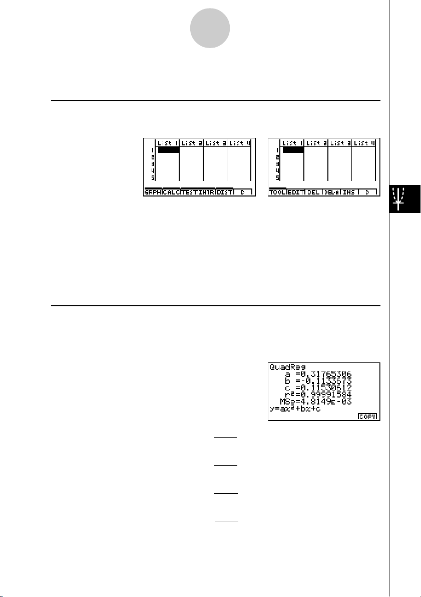
The following shows the function menus for the STAT Mode list input screen.
Pressing a function key that corresponds to the added item displays a menu that lets you
select one of the functions listed below.
• 3(TEST) ... Test (page1-2-1)
• 4(INTR) ... Confidence interval (page1-3-1)
• 5(DIST) ... Distribution (page1-4-1)
SORT and JUMP functions are located in the TOOL menu (6(g)1(TOOL)).
uu
uCalculation of the Coefficient of Determination (r2) and MSE
uu
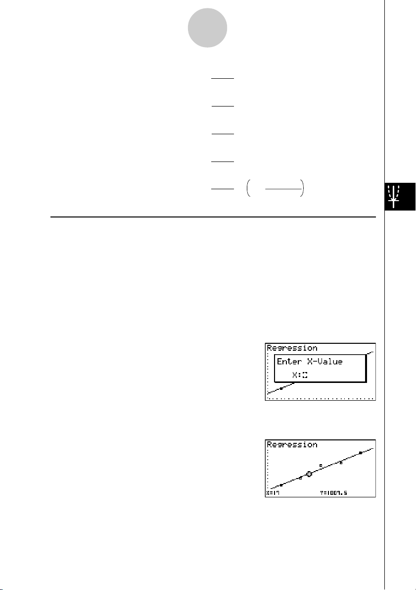
You can use the STAT Mode to calculate the coefficient of determination (r2) for quadratic
regression, cubic regression, and quartic regression. The following types of MSE
calculations are also available for each type of regression.
n
•Linear Regression ...
•Quadratic Regression ...
•Cubic Regression ...
•Quartic Regression ...
20010101
1
n – 2
1
n – 3
1
n – 4
1
n – 5
(yi – (axi+ b))
Σ
i=1
n
(yi – (ax
Σ
i=1
n
(yi – (ax
Σ
i=1
n
(yi – (ax
Σ
i=1
MSE =
MSE =
MSE =
MSE =
2
2
i
+ bxi+ c))
3
i
+ bx
i
4
i
+ bx
i3
2
+ cx
+ cx
2
i
+d ))
2
i
+ dx
2
i
+ e))
2
Page 7
1-1-2
Advanced Statistics (STAT)
n
• Logar ithmic Regression ...
•Exponential Repression ...
•Power Regression ...
•Sin Regression ...
• Logistic Regression ...
uu
uEstimated Value Calculation for Regression Graphs
uu
The STAT Mode also includes a Y-CAL function that uses regression to calculate the
estimated y-value for a particular x-value after graphing a paired-variable statistical
regression.
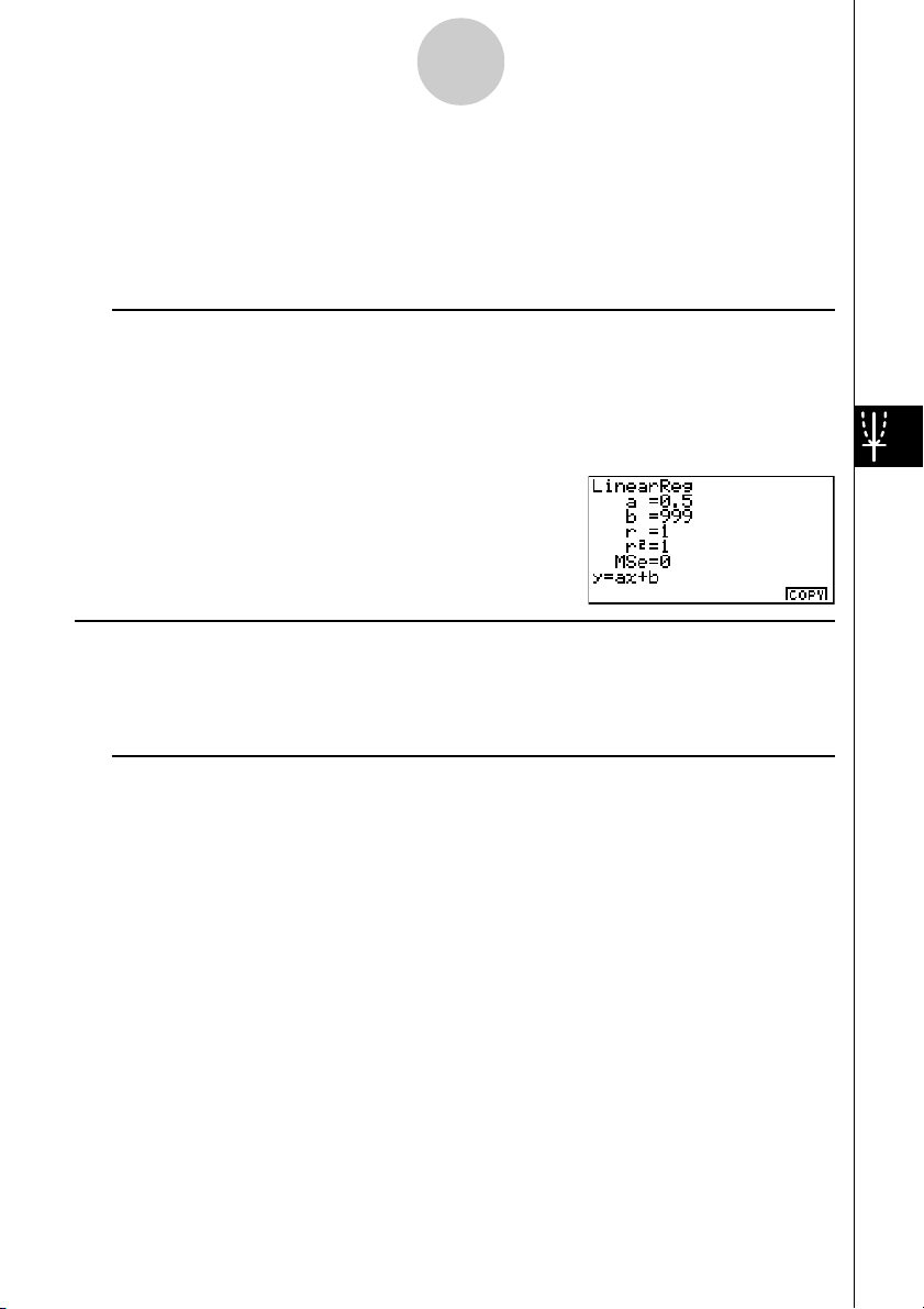
The following is the general procedure for using the Y-CAL function.
1. After drawing a regression graph, press 6(g)2(Y-CAL) to enter the graph selection mode,
and then press w.
If there are multiple graphs on the display, use f and c to select the graph you want, and
then press w.
• This causes an x-value input dialog box to appear.
MSE =
MSE =
MSE =
MSE =
MSE =
1
(yi – (a + b ln xi ))
Σ
n – 2
i=1
n
1
(ln yi – (ln a + bxi ))
Σ
n – 2
i=1
n
1
(ln yi – (ln a + b ln xi ))
Σ
n – 2
i=1
n
1
(yi – (a sin (bxi + c) + d ))
Σ
n – 2
i=1
n
1
n – 2 1 + ae
Σ
i=1
yi –
2
2
2
2
2
C
-bx
i
2. Input the value you want for x and then press w.
• This causes the coordinates for x and y to appear at the bottom of the display, and moves the
pointer to the corresponding point on the graph.
3. Pressing v or a number key at this time causes the x-value input dialog box to reappear
so you can perform another estimated value calculation if you want.
20010101
20011101
Page 8
1-1-3
Advanced Statistics (STAT)
4. After you are finished, press i to clear the coordinate values and the pointer from the
display.
· The pointer does not appear if the calculated coordinates are not within the display range.
·The coordinates do not appear if [Off] is specified for the [Coord] item of the [SETUP] screen.
· The Y-CAL function can also be used with a graph drawn by using DefG feature.
uu
u Regression Formula Copy Function from a Regression Calculation Result
uu
Screen
In addition to the normal regression formula copy function that lets you copy the regression
calculation result screen after drawing a statistical graph (such as Scatter Plot), the STAT Mode
also has a function that lets you copy the regression formula obtained as the result of a regression
calculation. To copy a resulting regression for mula, press 6(COPY).
kk
k Tests, Confidence Interval, and Distribution Calculations
kk
The STAT Mode includes functions for performing tests, and confidence interval and distribution
calculations. You can find explanations of each of these functions in the following sections: 1-2
Tests, 1-3 Confidence Interval, and 1-4 Distr ibution.
uu
uParameter Settings
uu
The following describes the two methods you can use to make parameter settings for test,
confidence interval, and distribution calculations.
• Selection
With this method, you press the function key that corresponds to the setting you want to
select from the function menu.
• Value Input
With this method, you directly input the parameter value you want to input. In this case,
nothing appears in the function menu.
·Pressing i returns to the list input screen, with the cursor in the same position it was at
before you started the parameter setting procedure.
· Pressing ! i(QUIT) returns to the top of list input screen.
· Pressing w without pressing 1(CALC) under “Execute” item advances to calculation
execution. To return to the parameter setting screen, press i, A, or w.
20010101
Page 9

1-1-4
Advanced Statistics (STAT)
uu
uCommon Functions
uu
• The symbol “■” appears in the upper right corner of the screen while execution of a
calculation is being performed and while a graph is being drawn. Pressing A during this
time terminates the ongoing calculation or draw operation (AC Break).
• Pressing i or w while a calculation result or graph is on the display returns to the
parameter setting screen. Pressing ! i(QUIT) returns to the top of list input screen.
· Pressing A while a calculation result is on the display returns to the parameter setting screen.
• Pressing u 5(G↔T) after drawing a graph switches to the parameter setting screen
(G↔T function). Pressing u 5(G↔T) again returns to the graph screen.
· The G↔T function is disabled whenever you change a setting on the parameter setting screen, or
when you perfor m a u 3(SET UP) or ! K(V-Window) operation.
• You can perform the PICT menu's screen save or recall functions after drawing a graph.
· The ZOOM function and SKETCH function are disabled.
The TRACE function is disabled, except for the graph display of two-way ANOVA.
The graph screen cannot be scrolled.
• After drawing a graph, you can use a Save Result feature to save calculation results to a
specific list. Basically, all items are saved as they are displayed, except for the first line title.
·Each time you execute Save Result, any existing data in the list is replaced by the new results.
20010101
20011101
Page 10

1-2-1
Tests (TEST)
1-2 Tests (TEST)
The Z Test provides a variety of different standardization-based tests. They make it possible
to test whether or not a sample accurately represents the population when the standard
deviation of a population (such as the entire population of a country) is known from previous
tests. Z testing is used for market research and public opinion research, that need to be
performed repeatedly.
1-Sample Z Test tests for the unknown population mean when the population standard
deviation is known.
2-Sample Z Test tests the equality of the means of two populations based on independent
samples when both population standard deviations are known.
1-Prop Z Test tests for an unknown proportion of successes.
2-Prop Z Test tests to compare the proportion of successes from two populations.
The t Test tests the hypothesis when the population standard deviation is unknown. The
hypothesis that is the opposite of the hypothesis being proven is called the
while the hypothesis being proved is called the
alternative hypothesis
applied to test the null hypothesis. Then a determination is made whether the null hypothesis
or alternative hypothesis will be adopted.
1-Sample t Test tests the hypothesis for a single unknown population mean when the
population standard deviation is unknown.
2-Sample t Test compares the population means when the population standard deviations
are unknown.
LinearReg t Test calculates the strength of the linear association of paired data.
null hypothesis
. The t-test is normally
,
2
χ
Test tests hypothesis concerning the proportion of samples included in each of a number
of independent groups. Mainly, it generates cross-tabulation of two categorical variables
(such as yes, no) and evaluates the independence of these variables. It could be used, for
example, to evaluate the relationship between whether or not a driver has ever been involved
in a traffic accident and that person’s knowledge of traffic regulations.
2-Sample F Test tests the hypothesis for the ratio of sample variances. It could be used, for
example, to test the carcinogenic effects of multiple suspected factors such as tobacco use,
alcohol, vitamin deficiency, high coffee intake, inactivity, poor living habits, etc.
ANOVA tests the hypothesis that the population means of the samples are equal when there
are multiple samples. It could be used, for example, to test whether or not different
combinations of materials have an effect on the quality and life of a final product.
One-Way ANOVA is used when there is one independent variable and one dependent
variable.
Two-Way ANOVA is used when there are two independent variables and one dependent
variable.
20010101
20011101
Page 11

1-2-2
Tests (TEST)
The following pages explain various statistical calculation methods based on the principles
described above. Details concerning statistical principles and terminology can be found in
any standard statistics textbook.
On the initial STAT Mode screen, press 3(TEST) to display the test menu, which contains
the following items.
• 3(TEST)b(Z) ... Z Tests (p. 1-2-2)
c(T) ... t Tests (p. 1-2-10)
d(χ2) ... χ2 Test (p. 1-2-18)
e(F) ... 2-Sample F Test (p. 1-2-20)
f(ANOVA) ... ANOVA (p. 1-2-22)
kk
k Z Tests
kk
uu
uZ Test Common Functions
uu
You can use the following graph analysis functions after drawing a graph.
• 1(Z) ... Displays z score.
Pressing 1 (Z) displays the z score at the bottom of the display, and displays the pointer at
the corresponding location in the graph (unless the location is off the graph screen).
Tw o points are displayed in the case of a two-tail test. Use d and e to move the pointer.
Press i to clear the z score.
• 2(P) ... Displays p-value.
Pressing 2 (P) displays the p-value at the bottom of the display without displaying the
pointer.
Press i to clear the p-value.
uu
u1-Sample Z Test
uu
This test is used when the population standard deviation is known to test the hypothesis. The
1-Sample Z Test is applied to the normal distribution.
µ
Z =
o –
σ
n
0
o : mean of sample
µ
o : assumed population mean
σ
: population standard deviation
n : s ize of sample
# The following V-Window settings are used for
drawing the graph.
Xmin = –3.2, Xmax = 3.2, Xscale = 1,
Ymin = –0.1, Ymax = 0.45, Yscale = 0.1
#Executing an analysis function automatically
stores the z and p values in alpha variables Z
and P, respectively.
20010101
20011101
Page 12

1-2-3
Tests (TEST)
Perform the following key operations from the statistical data list.
3(TEST)
b(Z)
b(1-Smpl)
The following shows the meaning of each item in the case of list data specification.
Data ............................ data type
µ
.................................. population mean value test conditions (“G
two-tail test, “<
µ
0” specifies lower one-tail test, “> µ0”
µ
0” specifies
specifies upper one-tail test.)
µ
0 ................................. assumed population mean
σ
.................................. population standard deviation (σ > 0)
List .............................. list whose contents you want to use as data (List 1 to 20)
Freq ............................. frequency (1 or List 1 to 20)
Save Res..................... list for storage of calculation results (None or List 1 to 20)
Execute ....................... executes a calculation or draws a graph
The following shows the meaning of parameter data specification items that are different
from list data specification.
o .................................. mean of sample
n .................................. size of sample (positive integer)
After setting all the parameters, align the cursor with [Execute] and then press one of the
function keys shown below to perform the calculation or draw the graph.
• 1(CALC) ... Performs the calculation.
• 6(DRAW) ... Draws the graph.
20010101
20011101
Page 13
Tests (TEST)
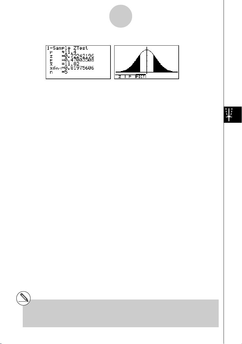
Calculation Result Output Example
µ
G11.4
........................
direction of test
z .................................. z score
p .................................. p-value
o .................................. mean of sample
x
σ
n-1 ............................. sample standard deviation
(Displayed only for Data: List setting.)
n .................................. size of sample
1-2-4
# [Save Res] does not save the µ condition in
line 2.
20010101
Page 14
1-2-5
Tests (TEST)
uu
u2-Sample Z Test
uu
This test is used when the standard deviations for two populations are known to test the
hypothesis. The 2-Sample Z T est is applied to the normal distribution.
Z =
o1 – o
2
σ
1
+
n
1
2
2
σ
2
n
2
o1 : mean of sample 1
o2 : mean of sample 2
σ
1 : population standard deviation of sample 1
σ
2 : population standard deviation of sample 2
n1 : siz e of sample 1
n2 : siz e of sample 2
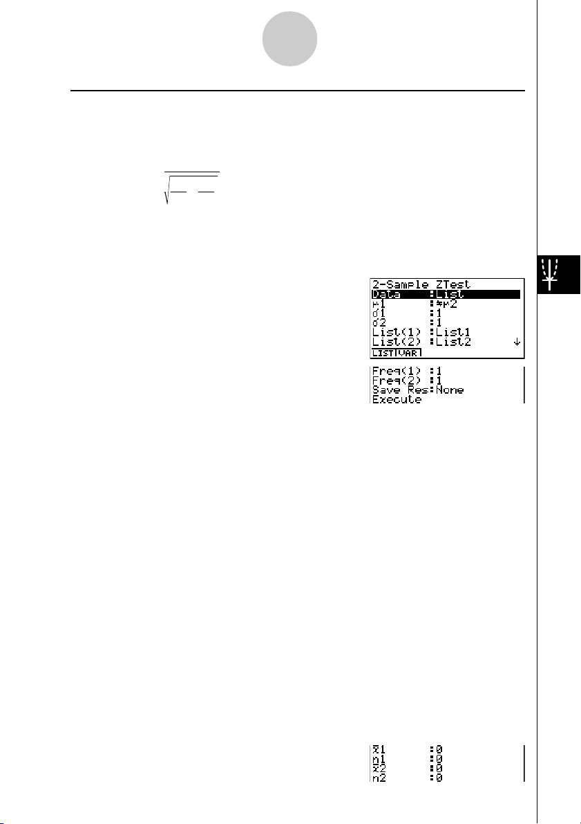
Perform the following key operations from the statistical data list.
3(TEST)
b(Z)
c(2-Smpl)
The following shows the meaning of each item in the case of list data specification.
Data ............................ data type
µ
1 ................................. population mean value test conditions (“G µ2” specifies two-
tail test, “<
smaller than sample 2, “>
µ
2” specifies one-tail test where sample 1 is
µ
2” specifies one-tail test where
sample 1 is greater than sample 2.)
σ
1 ................................. population standard deviation of sample 1 (σ1 > 0)
σ
2 ................................. population standard deviation of sample 2 (σ2 > 0)
List(1) .......................... list whose contents you want to use as sample 1 data
(List 1 to 20)
List(2) .......................... list whose contents you want to use as sample 2 data
(List 1 to 20)
Freq(1) ........................ frequency of sample 1 (1 or List 1 to 20)
Freq(2) ........................ frequency of sample 2 (1 or List 1 to 20)
Save Res..................... list for storage of calculation results (None or List 1 to 20)
Execute ....................... executes a calculation or draws a graph
The following shows the meaning of parameter data specification items that are different
from list data specification.
20010101
20011101
Page 15
1-2-6
Tests (TEST)
o1 ................................. mean of sample 1
n1 ................................. size (positive integer) of sample 1
o2 ................................. mean of sample 2
n2 ................................. size (positive integer) of sample 2
After setting all the parameters, align the cursor with [Execute] and then press one of the
function keys shown below to perform the calculation or draw the graph.
• 1(CALC) ... Performs the calculation.
• 6(DRAW) ... Draws the graph.
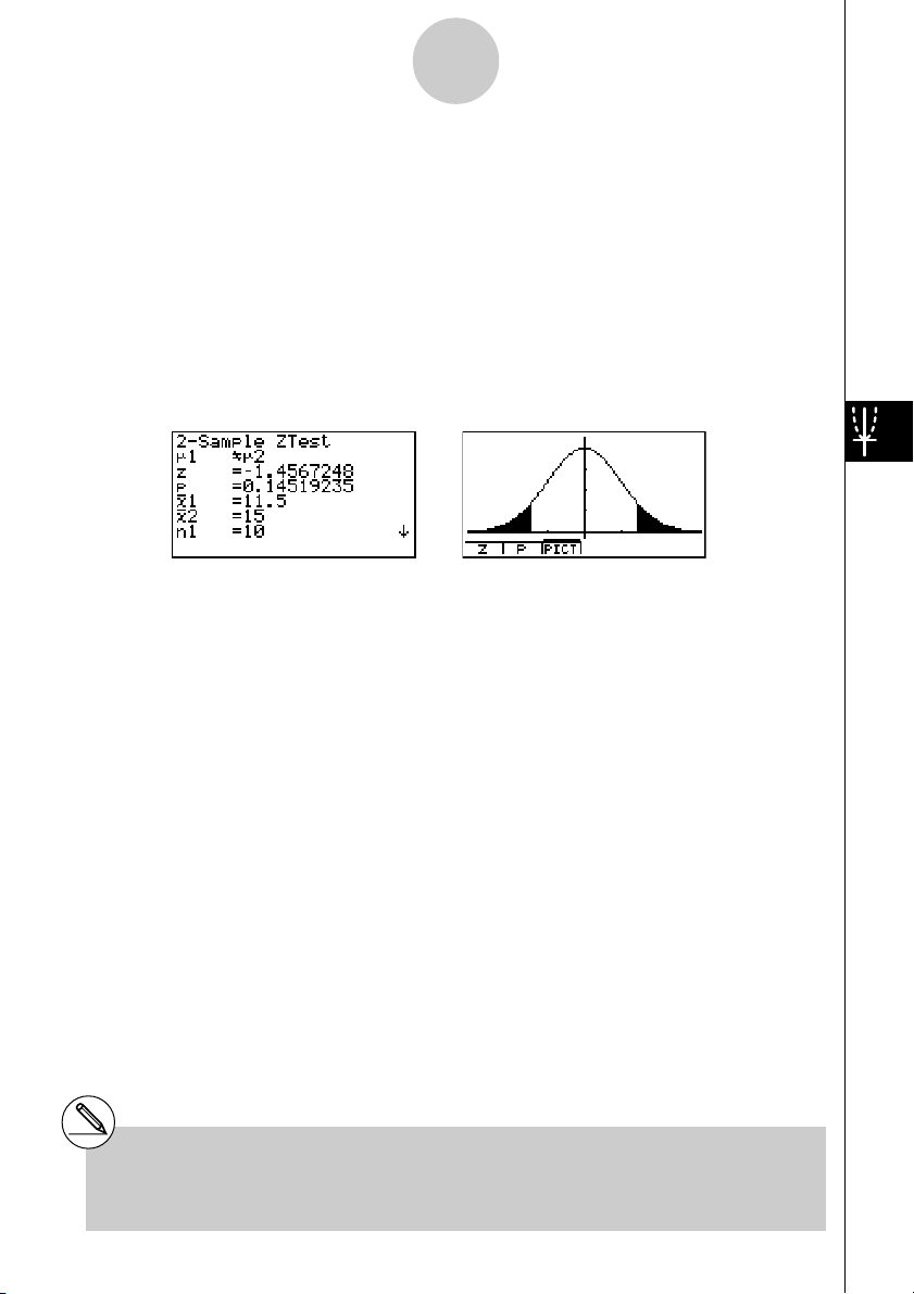
Calculation Result Output Example
µ
1
µ
2 ........................... direction of test
G
z ................................... z score
p .................................. p-value
o1 ................................. mean of sample 1
o2 ................................. mean of sample 2
x1
σ
n-1 ............................ standard deviation of sample 1
(Displayed only for Data: List setting.)
x2
σ
n-1 ............................ standard deviation of sample 2
(Displayed only for Data: List setting.)
n1 ................................. size of sample 1
n2 ................................. size of sample 2
# [Save Res] does not save the
line 2.
µ
1 condition in
20010101
Page 16
1-2-7
Tests (TEST)
uu
u1-Prop Z Test
uu
This test is used to test for an unknown proportion of successes. The 1-Prop Z Test is
applied to the normal distribution.
p0 : expected sample proportion
n : s ize of sample
Z =
x
n
p
(1– p0)
0
– p
0
n
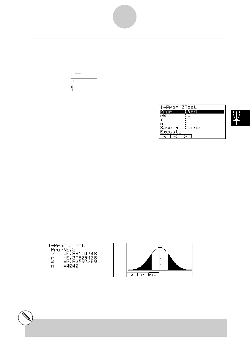
Perform the following key operations from the statistical data list.
3(TEST)
b(Z)
d(1-Prop)
Prop ............................ sample proportion test conditions (“G p0” specifies two-tail
test, “< p0” specifies lower one-tail test, “> p0” specifies upper
one-tail test.)
p0 ................................. expected sample proportion (0 < p0 < 1)
x .................................. sample value (x > 0 integer)
n .................................. size of sample (positive integer)
Save Res..................... list for storage of calculation results (None or List 1 to 20)
Execute ....................... executes a calculation or draws a graph
After setting all the parameters, align the cursor with [Execute] and then press one of the
function keys shown below to perform the calculation or draw the graph.
• 1(CALC) ... Performs the calculation.
• 6(DRAW) ... Draws the graph.
Calculation Result Output Example
PropG0.5 .................... direction of test
z ................................... z score
p .................................. p-value
ˆp .................................. estimated sample proportion
n .................................. size of sample
# [Save Res] does not save the Prop condition
in line 2.
20010101
20011101
Page 17
1-2-8
Tests (TEST)
uu
u2-Prop Z Test
uu
This test is used to compare the proportion of successes. The 2-Prop Z Test is applied to the
normal distribution.
x
x
2
1
–
n
n
2
p(1 – p )
1
1
1
+
n
n
2
1
Z =
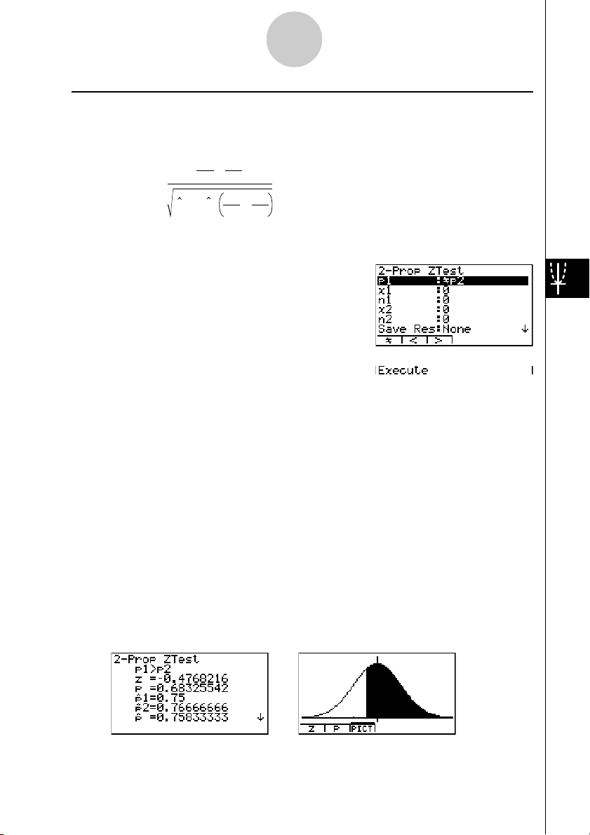
Perform the following key operation from the statistical data list.
3(TEST)
b(Z)
e(2-Prop)
x1 : data value of sample 1
x2 : data value of sample 2
n1 : siz e of sample 1
n2 : siz e of sample 2
ˆp : estimated sample proportion
p1 ................................. sample proportion test conditions (“G p2” specifies two-tail
test, “< p2” specifies one-tail test where sample 1 is smaller
than sample 2, “> p2” specifies one-tail test where sample 1
is greater than sample 2.)
x1 ................................. data value (x1 > 0 integer) of sample 1
n1 ................................. size (positive integer) of sample 1
x2 ................................. data value (x2 > 0 integer) of sample 2
n2 ................................. size (positive integer) of sample 2
Save Res..................... list for storage of calculation results (None or List 1 to 20)
Execute ....................... executes a calculation or draws a graph
After setting all the parameters, align the cursor with [Execute] and then press one of the
function keys shown below to perform the calculation or draw the graph.
• 1(CALC) ... Performs the calculation.
• 6(DRAW) ... Draws the graph.
Calculation Result Output Example
20010101
20011101
Page 18

1-2-9
Tests (TEST)
p1>p2 ............................ direction of test
z .................................. z score
p .................................. p-value
ˆp 1 ................................. estimated proportion of sample 1
ˆp 2 ................................. estimated proportion of sample 2
ˆp .................................. estimated sample proportion
n1 ................................. size of sample 1
n2 ................................. size of sample 2
# [Save Res] does not save the p1 condition in
line 2.
20010101
Page 19

1-2-10
Tests (TEST)
kk
k t Tests
kk
uu
u t Test Common Functions
uu
You can use the following graph analysis functions after drawing a graph.
• 1(T) ... Displays t score.
Pressing 1 (T) displays the t score at the bottom of the display, and displays the pointer at the
corresponding location in the graph (unless the location is off the graph screen).
Tw o points are displayed in the case of a two-tail test. Use d and e to move the pointer.
Press i to clear the t score.
• 2(P) ... Displays p-value.
Pressing 2 (P) displays the p-value at the bottom of the display without displaying the pointer.
Press i to clear the p-value.
# The following V-Window settings are used for
drawing the graph.
Xmin = –3.2, Xmax = 3.2, Xscale = 1,
Ymin = –0.1, Ymax = 0.45, Yscale = 0.1
#Executing an analysis function automatically
stores the t and p values in alpha variables T
and P, respectively.
20010101
Page 20
1-2-11
Tests (TEST)
uu
u1-Sample t Test
uu
This test uses the hypothesis test for a single unknown population mean when the population
standard deviation is unknown. The 1-Sample t T est is applied to t-distribution.
µ
t =
o –
σ
x
n
0
n–1
o : mean of sample
µ
0 : assumed population mean
x
σ
n-1 : sample standard deviation
n : siz e of sample
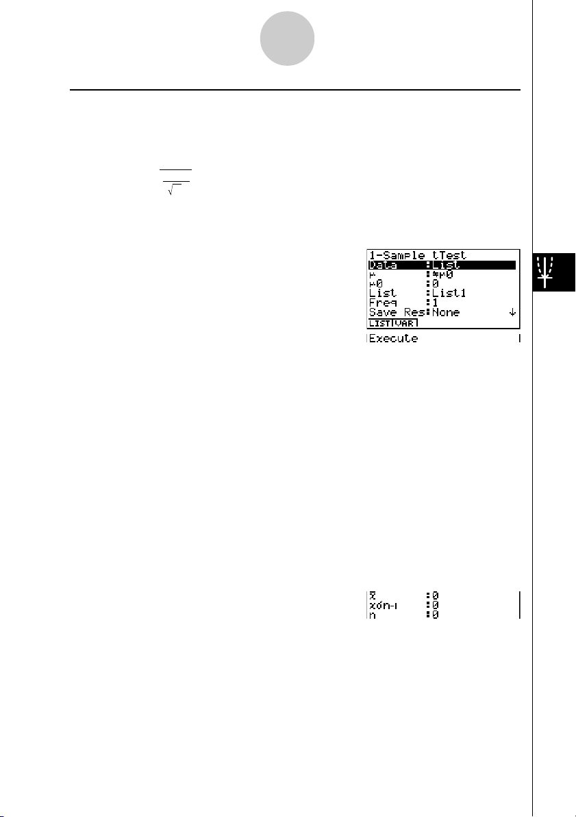
Perform the following key operations from the statistical data list.
3(TEST)
c(T)
b(1-Smpl)
The following shows the meaning of each item in the case of list data specification.
Data ............................ data type
µ
.................................. population mean value test conditions (“G
tail test, “<
µ
0” specifies lower one-tail test, “> µ0” specifies
upper one-tail test.)
µ
0 ................................. assumed population mean
List .............................. list whose contents you want to use as data (List 1 to 20)
Freq ............................. frequency (1 or List 1 to 20)
Save Res..................... list for storage of calculation results (None or List 1 to 20)
Execute ....................... executes a calculation or draws a graph
µ
0” specifies two-
The following shows the meaning of parameter data specification items that are different
from list data specification.
o .................................. mean of sample
x
σ
n-1 ............................. sample standard deviation (xσn-1 > 0)
n .................................. size of sample (positive integer)
After setting all the parameters, align the cursor with [Execute] and then press one of the
function keys shown below to perform the calculation or draw the graph.
• 1(CALC) ... Performs the calculation.
• 6(DRAW) ... Draws the graph.
20010101
20011101
Page 21

Calculation Result Output Example
µ
G 11.3 ...................... direction of test
t
...................................
t score
p .................................. p-value
o .................................. mean of sample
x
σ
n-1 ............................. sample standard deviation
n .................................. size of sample
1-2-12
Tests (TEST)
# [Save Res] does not save the µ condition in
line 2.
20010101
Page 22

1-2-13
Tests (TEST)
uu
u2-Sample t Test
uu
2-Sample t Test compares the population means when the population standard deviations
are unknown. The 2-Sample t Test is applied to t-distribution.
The following applies when pooling is in effect.
o1 – o
t
=
xp
=
x
σ
p n–1
df
= n1 + n2 – 2
2
1
1
2
n–1
+
n
n
2
1
(n
–1)x
1
σ
1
n
1
n–1
+ n
2
+(n2–1)x
– 2
2
σ
2
n–1
σ
The following applies when pooling is not in effect.
o1 – o
σ
1 n–1
n
1
2
C
σ
1 n–1
n
1
2
+
+
x
1 n–1
2
2
σ
x
2 n–1
n
1
(1–C )
n2–1
σ
n
1
x
+
2
2
σ
2 n–1
n
2
2
2
2
t =
x
df =
n1–1
C =
x
o1 :mean of sample 1
o2 :mean of sample 2
x1
σ
n-1 :standard deviation of
sample 1
x2
σ
2
n-1 :standard deviation of
sample 2
n1 :size of sample 1
n2 :size of sample 2
xp
σ
n-1 : pooled sample standard
deviation
df : degrees of freedom
o1 :mean of sample 1
o2 :mean of sample 2
x1
σ
n-1 :standard deviation of
sample 1
x2
σ
n-1 :standard deviation of
sample 2
n1 :size of sample 1
n2 :size of sample 2
df : degrees of freedom
Perform the following key operations from the statistical data list.
3(TEST)
c(T)
c(2-Smpl)
20010101
20011101
Page 23

1-2-14
Tests (TEST)
The following shows the meaning of each item in the case of list data specification.
Data ............................ data type
µ
1 ................................. sample mean value test conditions (“G µ2” specifies two-tail
test, “<
µ
2” specifies one-tail test where sample 1 is smaller
than sample 2, “>
µ
2” specifies one-tail test where sample 1 is
greater than sample 2.)
List(1) .......................... list whose contents you want to use as data of sample 1
(List 1 to 20)
List(2) .......................... list whose contents you want to use as data of sample 2
(List 1 to 20)
Freq(1) ........................ frequency of sample 1 (1 or List 1 to 20)
Freq(2) ........................ frequency of sample 2 (1 or List 1 to 20)
Pooled ......................... pooling On (in effect) or Off (not in effect)
Save Res..................... list for storage of calculation results (None or List 1 to 20)
Execute ....................... executes a calculation or draws a graph
The following shows the meaning of parameter data specification items that are different
from list data specification.
o1 ................................. mean of sample 1
x1
σ
n-1 ............................ standard deviation (x1σn-1 > 0) of sample 1
n1 ................................. size (positive integer) of sample 1
o2 ................................. mean of sample 2
x2
σ
n-1 ............................ standard deviation (x2σn-1 > 0) of sample 2
n2 ................................. size (positive integer) of sample 2
After setting all the parameters, align the cursor with [Execute] and then press one of the
function keys shown below to perform the calculation or draw the graph.
• 1(CALC) ... Performs the calculation.
• 6(DRAW) ... Draws the graph.
20010101
20011101
Page 24

Calculation Result Output Example
µ1Gµ
2 ........................... direction of test
t
...................................
t score
p .................................. p-value
df ................................. degrees of freedom
o1 ................................. mean of sample 1
o2 ................................. mean of sample 2
x1
σ
n-1 ............................ standard deviation of sample 1
x2
σ
n-1 ............................ standard deviation of sample 2
xp
σ
n-1 ............................ pooled sample standard deviation (Displayed only when Pooled:
On setting.)
n1 ................................. size of sample 1
n2 ................................. size of sample 2
1-2-15
Tests (TEST)
# [Save Res] does not save the
line 2.
µ1
condition in
20010101
Page 25

1-2-16
Tests (TEST)
uu
uLinearReg t T est
uu
LinearReg t Test treats paired-variable data sets as (x, y) pairs, and uses the method of
least squares to determine the most appropriate a, b coefficients of the data for the
regression formula y = a + bx. It also determines the correlation coefficient and t value, and
calculates the extent of the relationship between x and y.
b =
Σ
i=1
n
( x – o)( y – p)
n
(x – o)
Σ
i=1
2
a = p – bo t = r
n – 2
1 – r
a :intercept
b :slope of the line
n :size of sample (n > 3)
2
r : correlation coefficient
2
r
: coefficient of
determination
Perform the following key operations from the statistical data list.
3(TEST)
c(T)
d(LinReg)
The following shows the meaning of each item in the case of list data specification.
β
& ρ............................ p-value test conditions (“G 0” specifies two-tail test, “< 0”
specifies lower one-tail test, “> 0” specifies upper one-tail
test.)
XList ............................ list for x-axis data (List 1 to 20)
YList ............................ list for y-axis data (List 1 to 20)
Freq ............................. frequency (1 or List 1 to 20)
Save Res..................... list for storage of calculation results (None or List 1 to 20)
Execute ....................... executes a calculation
After setting all the parameters, align the cursor with [Execute] and then press the function key
shown below to perform the calculation.
• 1(CALC) ... Performs the calculation.
# You cannot draw a graph for LinearReg t
Test.
20010101
20011101
Page 26
1-2-17
Tests (TEST)
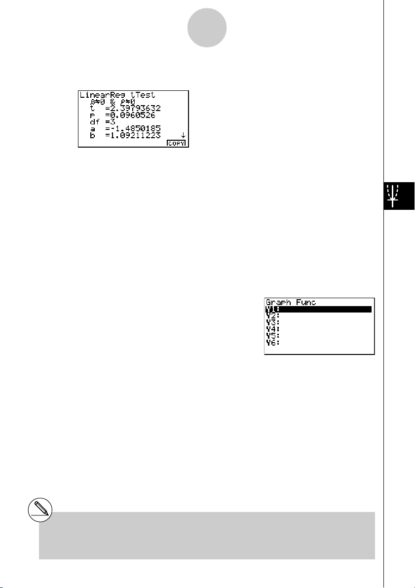
Calculation Result Output Example
β
G 0 &
ρ
G 0 .............. direction of test
t ................................... t score
p .................................. p-value
df ................................. degrees of freedom
a .................................. constant term
b .................................. coefficient
s .................................. standard error
r .................................. correlation coefficient
2
r
................................. coefficient of determination
Pressing 6 (COPY) while a calculation result is on the display copies the regression formula
to the graph formula editor.
When there is a list specified for the [Resid List] item on the SET UP screen, regression formula
residual data is automatically saved to the specified list after the calculation is finished.
# [Save Res] does not save the β &
conditions in line 2.
ρ
#When the list specified by [Save Res] is the
same list specified by the [Resid List] item on
the SET UP screen, only [Resid List] data is
saved in the list.
20010101
Page 27

j
1-2-18
Tests (TEST)
kk
k χ2 Test
kk
χ2 Test sets up a number of independent groups and tests hypothesis related to the
proportion of the sample included in each group. The χ2 Test is applied to dichotomous
variables (variable with two possible values, such as yes/no).
Fij =
χ2 =
k
x
Σ
i=1
ΣΣ
i=1
k
ΣΣ
i=1
×
ij
Σ
j=1
k
j=1
(xij – Fij)
=1
x
ij
x
ij
2
F
ij
Expected counts
Perform the following key operations from the statistical data list.
3(TEST)
d(χ2)
Next, specify the matrix that contains the data. The following shows the meaning of the
above item.
Observed .................... name of matrix (A to Z) that contains observed counts (all cells
positive integers)
Expected ..................... name of matrix (A to Z) that is for saving expected frequency
Save Res..................... list for storage of calculation results (None or List 1 to 20)
Execute ....................... executes a calculation or draws a graph
# The matrix must be at least two lines by two
columns. An error occurs if the matrix has
only one line or one column.
#Pressing 2 ('MAT) while setting
parameters enters the MATRIX editor, which
you can use to edit and view the contents of
matrices.
20010101
20011101
Page 28

1-2-19
Tests (TEST)
After setting all the parameters, align the cursor with [Execute] and then press one of the
function keys shown below to perform the calculation or draw the graph.
• 1(CALC) ... Performs the calculation.
• 6(DRAW) ... Draws the graph.
Calculation Result Output Example
2
χ
................................. χ2 value
p .................................. p-value
df ................................. degrees of freedom
You can use the following graph analysis functions after drawing a graph.
• 1(CHI) ... Displays
Pressing 1 (CHI) displays the
2
χ
value.
2
χ
value at the bottom of the display, and displays the pointer at
the corresponding location in the graph (unless the location is off the graph screen).
Press i to clear the
2
χ
value.
• 2(P) ... Displays p-value.
Pressing 2 (P) displays the p-value at the bottom of the display without displaying the pointer.
Press i to clear the p-value.
# Pressing 6('MAT) while a calculation
result is displayed enters the MATRIX editor,
which you can use to edit and view the
contents of matrices.
# The following V-Window settings are used for
drawing the graph.
Xmin = 0, Xmax = 11.5, Xscale = 2,
Ymin = –0.1, Ymax = 0.5, Yscale = 0.1
#Executing an analysis function automatically
stores the
C and P, respectively.
20010101
2
χ
and p values in alpha variables
Page 29

1-2-20
Tests (TEST)
kk
k 2-Sample F Test
kk
2-Sample F Test tests the hypothesis for the ratio of sample variances. The F Test is applied
to the F distribution.
F =
x
σ
2 n–1
2
2
σ
x
1 n–1
Perform the following key operations from the statistical data list.
3(TEST)
e(F)
The following is the meaning of each item in the case of list data specification.
Data ............................ data type
σ
1 ................................. population standard deviation test conditions (“G σ2”
specifies two-tail test, “<
sample 1 is smaller than sample 2, “>
σ
2” specifies one-tail test where
σ
2” specifies one-tail
test where sample 1 is greater than sample 2.)
List(1) .......................... list whose contents you want to use as data of sample 1
(List 1 to 20)
List(2) .......................... list whose contents you want to use as data of sample 2
(List 1 to 20)
Freq(1) ........................ frequency of sample 1 (1 or List 1 to 20)
Freq(2) ........................ frequency of sample 2 (1 or List 1 to 20)
Save Res..................... list for storage of calculation results (None or List 1 to 20)
Execute ....................... executes a calculation or draws a graph
The following shows the meaning of parameter data specification items that are different
from list data specification.
x1
σ
n-1 ............................ standard deviation (x1σn-1
>
0) of sample 1
n1 ................................. size (positive integer) of sample 1
x2
σ
n-1 ............................ standard deviation (x2σn-1
>
0) of sample 2
n2 ................................. size (positive integer) of sample 2
20010101
20011101
Page 30

1-2-21
Tests (TEST)
After setting all the parameters, align the cursor with [Execute] and then press one of the
function keys shown below to perform the calculation or draw the graph.
• 1(CALC) ... Performs the calculation.
• 6(DRAW) ... Draws the graph.
Calculation Result Output Example
σ1Gσ
2 .......................... direction of test
F.................................. F value
p .................................. p-value
o1 ................................. mean of sample 1 (Displayed only for Data: List setting.)
o2 ................................. mean of sample 2 (Displayed only for Data: List setting.)
x1
σ
n-1 ............................ standard deviation of sample 1
x2
σ
n-1 ............................ standard deviation of sample 2
n1 ................................. size of sample 1
n2 ................................. size of sample 2
You can use the following graph analysis functions after drawing a graph.
• 1(F) ... Displays F value.
Pressing 1 (F) displays the F value at the bottom of the display, and displays the pointer at
the corresponding location in the graph (unless the location is off the graph screen).
Tw o points are displayed in the case of a two-tail test. Use d and e to move the pointer.
Press i to clear the F value.
• 2(P) ... Displays p-value.
Pressing 2 (P) displays the p-value at the bottom of the display without displaying the pointer.
Press i to clear the p-value.
# [Save Res] does not save the
line 2.
# V-Window settings are automatically
optimized for drawing the graph.
σ
1 condition in
#Executing an analysis function automatically
stores the
F and P, respectively.
20010101
F and p values in alpha variables
Page 31

1-2-22
Tests (TEST)
kk
k ANOVA
kk
ANOVA tests the hypothesis that the population means of the samples are equal when there
are multiple samples.
One-Way ANOVA is used when there is one independent variable and one dependent
variable.
Two-Way ANOVA is used when there are two independent variables and one dependent
variable.
Perform the following key operations from the statistical data list.
3(TEST)
f(ANOVA)
The following is the meaning of each item in the case of list data specification.
How Many ................... selects One-Way ANOVA or Two-Way ANOVA (number of
levels)
Factor A....................... category list (List 1 to 20)
Dependnt .................... list to be used for sample data (List 1 to 20)
Save Res..................... first list for storage of calculation results (None or List 1 to
16)*
1
Execute ....................... executes a calculation or draws a graph (Two-Way ANOVA only)
The following item appears in the case of Two-Way ANOVA only.
Factor B....................... category list (List 1 to 20)
After setting all the parameters, align the cursor with [Execute] and then press one of the
function keys shown below to perform the calculation or draw the graph.
• 1(CALC) ... Performs the calculation.
• 6(DRAW) ... Draws the graph (Two-Way ANOVA only).
Calculation results are displayed in table form, just as they appear in science books.
*1 [Save Res] saves each vertical column of the
table into its own list. The leftmost column is
saved in the specified list, and each
subsequent column to the right is saved in
the next sequentially numbered list. Up to five
lists can be used for storing columns. You
can specify an first list number in the range of
1 to 16.
20010101
20011101
Page 32

1-2-23
Tests (TEST)
Calculation Result Output Example
One-Way ANOVA
Line 1 (A) .................... Factor A df value, SS value, MS value, F value, p-value
Line 2 (ERR) ............... Error df value, SS value, MS value
Tw o- Wa y ANOVA
Line 1 (A) .................... Factor A df value, SS value, MS value, F value, p-value
Line 2 (B) .................... Factor B df value, SS value, MS value, F value, p-value
Line 3 (AB) .................. Factor A × Factor B df value, SS value, MS value, F value,
p-value
*Line 3 does not appear when there is only one observation
in each cell.
Line 4 (ERR) ............... Error df value, SS value, MS value
F.................................. F value
p .................................. p-value
df ................................. degrees of freedom
SS ................................ sum of squares
MS............................... mean squares
With Two-Way ANOVA, you can draw Interaction Plot graphs. The number of graphs depends
on Factor B, while the number of X-axis data depends on the Factor A. The Y-axis is the average
value of each category.
You can use the following graph analysis function after drawing a graph.
• 1(TRACE) ... Trace function
Pressing d or e moves the pointer on the graph in the corresponding direction. When there
are multiple graphs, you can move between graphs by pressing f and c.
Press i to clear the pointer from the display.
# Graphing is available with Two-Way ANOVA
only. V-Window settings are performed
automatically, regardless of SET UP screen
settings.
# Using the TRACE function automatically
stores the number of conditions to alpha
variable A and the mean value to variable M,
respectively.
20010101
Page 33

1-2-24
Tests (TEST)
kk
k ANOVA (Two-Way)
kk
uu
uDescription
uu
The nearby table shows measurement results for a metal product produced by a heat
treatment process based on two treatment levels: time (A) and temperature (B). The
experiments were repeated twice each under identical conditions.
B (Heat Treatment Temperature) B1 B2
A (Time)
A1 113 , 116
A2
133 , 131
139 , 132
126 , 122
Perform analysis of variance on the following null hypothesis, using a significance level of
5%.
Ho : No change in strength due to time
Ho : No change in strength due to heat treatment temperature
Ho : No change in strength due to interaction of time and heat treatment temperature
uu
uSolution
uu
Use two-way ANOVA to test the above hypothesis.
Input the above data as shown below.
List1={1,1,1,1,2,2,2,2}
List2={1,1,2,2,1,1,2,2}
List3={113,116,139,132,133,131,126,122 }
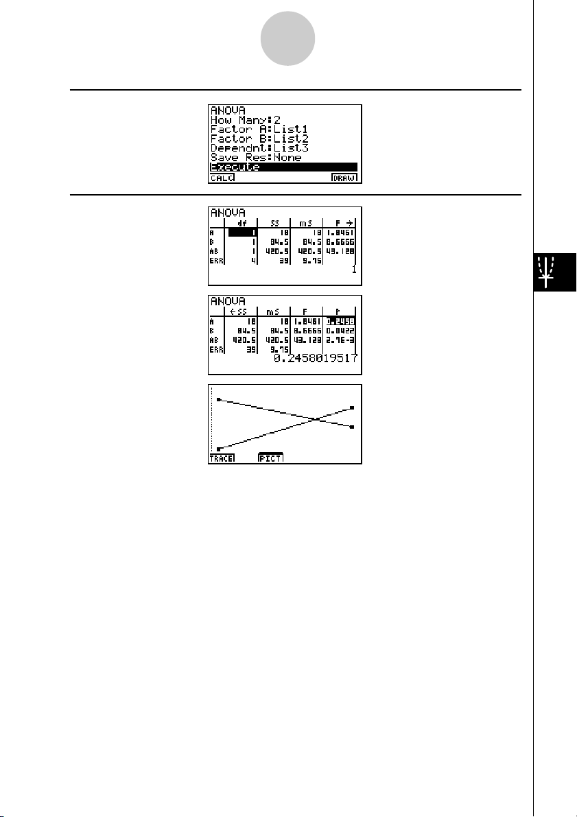
Define List 3 (the data for each group) as Dependent. Define List 1 and List 2 (the factor
numbers for each data item in List 3) as Factor A and Factor B respectively.
Executing the test produces the following results.
•Time differential (A) level of significance P = 0.2458019517
The level of significance (p = 0.2458019517) is greater than the significance level (0.05),
so the hypothesis is not rejected.
•Temperature differential (B) level of significance P = 0.04222398836
The level of significance (p = 0.04222398836) is less than the significance level (0.05), so
the hypothesis is rejected.
•Interaction (A × B) level of significance P = 2.78169946e-3
The level of significance (p = 2.78169946e-3) is less than the significance level (0.05), so
the hypothesis is rejected.
The above test indicates that the time differential is not significant, the temperature
differential is significant, and interaction is highly significant.
20010101
20011101
Page 34
uu
uInput Example
uu
uu
uResults
uu
1-2-25
Tests (TEST)
20010101
Page 35

1-3-1
Confidence Interval (INTR)
1-3 Confidence Interval (INTR)
A confidence interval is a range (interval) that includes a statistical value, usually the
population mean.
A confidence interval that is too broad makes it difficult to get an idea of where the population
value (true value) is located. A narrow confidence interval, on the other hand, limits the
population value and makes it difficult to obtain reliable results. The most commonly used
confidence levels are 95% and 99%. Raising the confidence level broadens the confidence
interval, while lowering the confidence level narrows the confidence level, but it also
increases the chance of accidently overlooking the population value. With a 95% confidence
interval, for example, the population value is not included within the resulting intervals 5% of
the time.
When you plan to conduct a survey and then t test and Z test the data, you must also
consider the sample size, confidence interval width, and confidence level. The confidence
level changes in accordance with the application.
1-Sample Z Interval calculates the confidence interval for an unknown population mean
when the population standard deviation is known.
2-Sample Z Interval calculates the confidence interval for the difference between two
population means when the population standard deviations of two samples are known.
1-Prop Z Interval calculates the confidence interval for an unknown proportion of
successes.
2-Prop Z Interval calculates the confidence interval for the difference between the propotion
of successes in two populations.
1-Sample t Interval calculates the confidence interval for an unknown population mean
when the population standard deviation is unknown.
2-Sample t Interval calculates the confidence interval for the difference between two
population means when both population standard deviations are unknown.
On the initial STAT Mode screen, press 4 (INTR) to display the confidence interval menu,
which contains the following items.
• 4(INTR)b(Z) ... Z intervals (p. 1-3-3)
c(T) ... t intervals (p. 1-3-8)
# There is no graphing for confidence interval
functions.
20010101
20011101
Page 36

1-3-2
Confidence Interval (INTR)
uu
uGeneral Confidence Interval Precautions
uu
Inputting a value in the range of 0 < C-Level < 1 for the C-Level setting sets you value you
input. Inputting a value in the range of 1 < C-Level < 100 sets a value equivalent to your input
divided by 100.
# Inputting a value of 100 or greater, or a
negative value causes an error (Ma ERROR).
20010101
Page 37

1-3-3
Confidence Interval (INTR)
kk
k Z Interval
kk
uu
u1-Sample Z Interval
uu
1-Sample Z Interval calculates the confidence interval for an unknown population mean
when the population standard deviation is known.
The following is the confidence interval.
α
Left = o – Z
Right = o + Z
However, α is the level of significance. The value 100 (1 – α) % is the confidence level.
When the confidence level is 95%, for example, inputting 0.95 produces 1 – 0.95 = 0.05 = α.
Perform the following key operations from the statistical data list.
4(INTR)
b(Z)
b(1-Smpl)
σ
2
n
α
σ
2
n
The following shows the meaning of each item in the case of list data specification.
Data ............................ data type
C-Level ........................ confidence level (0 < C-Level < 1)
σ
.................................. population standard deviation (σ > 0)
List .............................. list whose contents you want to use as sample data
(List 1 to 20)
Freq ............................. sample frequency (1 or List 1 to 20)
Save Res..................... list for storage of calculation results (None or List 1 to 20)
Execute ....................... executes a calculation
The following shows the meaning of parameter data specification items that are different
from list data specification.
o .................................. mean of sample
n .................................. size of sample (positive integer)
20010101
20011101
Page 38

1-3-4
Confidence Interval (INTR)
After setting all the parameters, align the cursor with [Execute] and then press the function
key shown below to perform the calculation.
• 1(CALC) ... Performs the calculation.
Calculation Result Output Example
Left .............................. inter val lower limit (left edge)
Right ............................ interval upper limit (right edge)
o .................................. mean of sample
x
σ
n-1 ............................. sample standard deviation
(Displayed only for Data: List setting.)
n .................................. size of sample
uu
u 2-Sample Z Interval
uu
2-Sample Z Interval calculates the confidence interval for the difference between two
population means when the population standard deviations of two samples are known.
The following is the confidence interval. The value 100 (1 –
2
2
σ
Left = (o1 – o2) – Z
Right = (o
– o2) + Z
1
α
2
α
2
σ
1
2
+
n
n
1
2
2
σ
σ
1
+
n
n
1
α) % is the confidence level.
o1 :mean of sample 1
o2 :mean of sample 2
σ
2
2
2
1 : population standard deviation
σ
2 : population standard deviation
of sample 1
of sample 2
n1 :size of sample 1
n2 :size of sample 2
Perform the following key operations from the statistical data list.
4(INTR)
b(Z)
c(2-Smpl)
20010101
2001010120011101
Page 39

1-3-5
Confidence Interval (INTR)
The following shows the meaning of each item in the case of list data specification.
Data ............................ data type
C-Level ........................ confidence level (0 < C-Level < 1)
σ
1 ................................. population standard deviation of sample 1 (σ1 > 0)
σ
2 ................................. population standard deviation of sample 2 (σ2 > 0)
List(1) .......................... list whose contents you want to use as data of sample 1
(List 1 to 20)
List(2) .......................... list whose contents you want to use as data of sample 2
(List 1 to 20)
Freq(1) ........................ frequency of sample 1 (1 or List 1 to 20)
Freq(2) ........................ frequency of sample 2 (1 or List 1 to 20)
Save Res..................... list for storage of calculation results (None or List 1 to 20)
Execute ....................... executes a calculation
The following shows the meaning of parameter data specification items that are different
from list data specification.
o1 ................................. mean of sample 1
n1 ................................. size (positive integer) of sample 1
o2 ................................. mean of sample 2
n2 ................................. size (positive integer) of sample 2
After setting all the parameters, align the cursor with [Execute] and then press the function
key shown below to perform the calculation.
• 1(CALC) ... Performs the calculation.
Calculation Result Output Example
Left .............................. inter val lower limit (left edge)
Right ............................ interval upper limit (right edge)
o1 ................................. mean of sample 1
o2 ................................. mean of sample 2
x1
σ
n-1 ............................ standard deviation of sample 1
(Displayed only for Data: List setting.)
x2
σ
n-1 ............................ standard deviation of sample 2
(Displayed only for Data: List setting.)
n1 ................................. size of sample 1
n2 ................................. size of sample 2
20010101
20011101
Page 40

1-3-6
Confidence Interval (INTR)
uu
u1-Prop Z Interval
uu
1-Prop Z Interval uses the number of data to calculate the confidence interval for an
unknown proportion of successes.
The following is the confidence interval. The value 100 (1 –
x
Left = – Z
n
Right = + Z
Perform the following key operations from the statistical data list.
4(INTR)
b(Z)
d(1-Prop)
Data is specified using parameter specification. The following shows the meaning of each
item.
C-Level ........................ confidence level (0 < C-Level < 1)
x
n
α
2
α
2
1
n
nxn
n1nxn
1–
1–
x
x
α) % is the confidence level.
n :size of sample
x : data
x .................................. data (0 or positive integer)
n .................................. size of sample (positive integer)
Save Res..................... list for storage of calculation results (None or List 1 to 20)
Execute ....................... executes a calculation
After setting all the parameters, align the cursor with [Execute] and then press the function
key shown below to perform the calculation.
• 1(CALC) ... Performs the calculation.
Calculation Result Output Example
Left .............................. inter val lower limit (left edge)
Right ............................ interval upper limit (right edge)
ˆp .................................. estimated sample propor tion
n .................................. size of sample
20010101
20011101
Page 41

1-3-7
Confidence Interval (INTR)
uu
u 2-Prop Z Interval
uu
2-Prop Z Interval uses the number of data items to calculate the confidence interval for the
defference between the proportion of successes in two populations.
The following is the confidence interval. The value 100 (1 –
x
x
1
1
1–
n
n
1
x
x
1
Left = – – Z
Right = – + Z
2
n
n
1
2
x
x
1
2
n
n
1
2
1
α
2
α
2
+
n
1
x
x
1
1
1–
n
n
1
1
n
1
α) % is the confidence level.
x
x
2
1–
n
n
2
n
2
x
2
1–
n
2
+
n
2
n1, n2 : s i ze of sample
2
x1, x2 : data
2
x
2
n
2
Perform the following key operations from the statistical data list.
4(INTR)
b(Z)
e(2-Prop)
Data is specified using parameter specification. The following shows the meaning of each
item.
C-Level ........................ confidence level (0 < C-Level < 1)
x1 ................................. data value (x1 > 0) of sample 1
n1 ................................. size (positive integer) of sample 1
x2 ................................. data value (x2 > 0) of sample 2
n2 ................................. size (positive integer) of sample 2
Save Res..................... list for storage of calculation results (None or List 1 to 20)
Execute ....................... executes a calculation
After setting all the parameters, align the cursor with [Execute] and then press the function
key shown below to perform the calculation.
• 1(CALC) ... Performs the calculation.
Calculation Result Output Example
20010101
20011101
Page 42

1-3-8
Confidence Interval (INTR)
Left .............................. inter val lower limit (left edge)
Right ............................ interval upper limit (right edge)
ˆp 1 ................................. estimated sample propotion for sample 1
ˆp 2 ................................. estimated sample propotion for sample 2
n1 ................................. size of sample 1
n2 ................................. size of sample 2
kk
k t Interval
kk
uu
u 1-Sample t Interval
uu
1-Sample t Interval calculates the confidence interval for an unknown population mean
when the population standard deviation is unknown.
The following is the confidence interval. The value 100 (1 –
Left = o– t
n – 1
Right = o+ t
Perform the following key operations from the statistical data list.
4(INTR)
c(T)
b(1-Smpl)
n – 1
σ
x
α
n–1
n
2
x
σ
α
n–1
n
2
α) % is the confidence level.
The following shows the meaning of each item in the case of list data specification.
Data ............................ data type
C-Level ........................ confidence level (0 < C-Level < 1)
List .............................. list whose contents you want to use as sample data
(List 1 to 20)
Freq ............................. sample frequency (1 or List 1 to 20)
Save Res..................... list for storage of calculation results (None or List 1 to 20)
Execute ....................... executes a calculation
The following shows the meaning of parameter data specification items that are different
from list data specification.
20010101
20011101
Page 43

1-3-9
Confidence Interval (INTR)
o .................................. mean of sample
x
σ
n-1 ............................. sample standard deviation (xσn-1 > 0)
n .................................. size of sample (positive integer)
After setting all the parameters, align the cursor with [Execute] and then press the function
key shown below to perform the calculation.
• 1(CALC) ... Performs the calculation.
Calculation Result Output Example
Left .............................. inter val lower limit (left edge)
Right ............................ interval upper limit (right edge)
o .................................. mean of sample
x
σ
n-1 ............................. sample standard deviation
n .................................. size of sample
uu
u 2-Sample t Interval
uu
2-Sample t Interval calculates the confidence interval for the difference between two
population means when both population standard deviations are unknown. The t interval is
applied to t distribution.
The following confidence interval applies when pooling is in effect. The value 100 (1 –
α) % is
the confidence level.
Left = (o1 – o2)– t
Right = (o
x
σ
p n–1
=
– o2)+ t
1
(n
–1)x
1
n1+n
1
n
n1+n
σ
–2
2
n–1
+ n
1
α
2
α
–2
2
2
2
+(n2–1)x
– 2
2
20010101
20011101
xp
xp
σ
n–1
σ
2
1
1
2
+
n
n
2
1
1
1
2
+
n–1
σ
n–1
n
n
2
1
2
Page 44

1-3-10
Confidence Interval (INTR)
The following confidence interval applies when pooling is not in effect. The value
100 (1 –
α) % is the confidence level.
Left = (o1 – o2)– t
C
n1–1
σ
x
1 n–1
n
1
2
x
1
– o2)+ t
1
(1–C)
+
n2–1
σ
1 n–1
n
1
2
x
2 n–1
+
Right = (o
df =
C =
2
σ
x
α
df
2
σ
n
2
1 n–1
n
2
df
2
2
1
σ
x
α
1 n–1
n
2
1
2
σ
x
2 n–1
+
n
2
2
2
σ
x
2 n–1
+
n
2
Perform the following key operations from the statistical data list.
4(INTR)
c(T)
c(2-Smpl)
The following shows the meaning of each item in the case of list data specification.
Data ............................ data type
C-Level ........................ confidence level (0 < C-Level < 1)
List(1) .......................... list whose contents you want to use as data of sample 1
(List 1 to 20)
List(2) .......................... list whose contents you want to use as data of sample 2
(List 1 to 20)
Freq(1) ........................ frequency of sample 1 (1 or List 1 to 20)
Freq(2) ........................ frequency of sample 2 (1 or List 1 to 20)
Pooled ......................... pooling On (in effect) or Off (not in effect)
Save Res..................... list for storage of calculation results (None or List 1 to 20)
Execute ....................... executes a calculation
The following shows the meaning of parameter data specification items that are different
from list data specification.
20010101
20011101
Page 45

1-3-11
Confidence Interval (INTR)
o1 ................................. mean of sample 1
x1
σ
n-1 ............................ standard deviation (x1σn-1 > 0) of sample 1
n1 ................................. size (positive integer) of sample 1
o2 ................................. mean of sample 2
x2
σ
n-1 ............................ standard deviation (x2σn-1 > 0) of sample 2
n2 ................................. size (positive integer) of sample 2
After setting all the parameters, align the cursor with [Execute] and then press the function
key shown below to perform the calculation.
• 1(CALC) ... Performs the calculation.
Calculation Result Output Example
Left .............................. inter val lower limit (left edge)
Right ............................ interval upper limit (right edge)
df ................................. degrees of freedom
o1 ................................. mean of sample 1
o2 ................................. mean of sample 2
x1
σ
n-1 ............................ standard deviation of sample 1
x2
σ
n-1 ............................ standard deviation of sample 2
xp
σ
n-1 ............................ pooled sample standard deviation
(Displayed only when Pooled: On setting.)
n1 ................................. size of sample 1
n2 ................................. size of sample 2
20010101
Page 46

1-4-1
Distribution (DIST)
1-4 Distribution (DIST)
There is a variety of different types of distribution, but the most well-known is “normal
distribution,” which is essential for performing statistical calculations. Normal distribution is a
symmetrical distribution centered on the greatest occurrences of mean data (highest
frequency), with the frequency decreasing as you move away from the center. Poisson
distribution, geometric distribution, and various other distribution shapes are also used,
depending on the data type.
Certain trends can be determined once the distr ibution shape is determined. You can
calculate the probability of data taken from a distribution being less than a specific value.
For example, distribution can be used to calculate the yield rate when manufacturing some
product. Once a value is established as the criteria, you can calculate normal probability
when estimating what percent of the products meet the criteria. Conversely, a success rate
target (80% for example) is set up as the hypothesis, and normal distribution is used to
estimate the proportion of the products will reach this value.
Normal probability density calculates the probability density of normal distribution from a
specified x value.
Normal distribution probability calculates the probability of normal distribution data falling
between two specific values.
Inverse cumulative normal distribution calculates a value that represents the location
within a normal distribution for a specific cumulative probability.
Student- t probability density calculates t probability density from a specified x value.
Student- t distribution probability calculates the probability of t distribution data falling
between two specific values.
Like t distribution, distribution probability can also be calculated for χ2, F, Binomial, Poisson,
and Geometric distributions.
On the initial STAT Mode screen, press 5 (DIST) to display the distribution menu, which
contains the following items.
• 5(DIST)b(Norm) ... Normal distribution (p. 1-4-3)
c(T) ... Student-t distribution (p. 1-4-7)
d(χ2) ... χ2 distribution (p. 1-4-9)
e(F) ... F distribution (p. 1-4-12)
f(Binmal) ... Binomial distribution (p. 1-4-16)
g(Poissn) ... Poisson distribution (p. 1-4-19)
h(Geo) ... Geometric distribution (p. 1-4-21)
20010101
Page 47

1-4-2
Distribution (DIST)
uu
uCommon Distribution Functions
uu
After drawing a graph, you can use the P-CAL function to calculate an estimated p-value for
a particular x value.
The following is the general procedure for using the P-CAL function.
1. After drawing a graph, press 1 (P-CAL) to display the x value input dialog box.
2. Input the value you want for x and then press w.
• This causes the x and p values to appear at the bottom of the display, and moves the
pointer to the corresponding point on the graph.
3. Pressing v or a number key at this time causes the x value input dialog box to reappear
so you can perform another estimated value calculation if you want.
4. After you are finished, press i to clear the coordinate values and the pointer from the
display.
# Executing an analysis function automatically
stores the x and p values in alpha variables X
and P, respectively.
20010101
Page 48

1-4-3
Distribution (DIST)
kk
k Normal Distribution
kk
uu
uNormal Probability Density
uu
Normal probability density calculates the probability density of nomal distribution from a
specified x value. Normal probability density is applied to standard normal distribution.
2
µ
(x – µ)
–
f(x) =
1
2
πσ
2
2
σ
e
(σ > 0)
Perform the following key operations from the statistical data list.
5(DIST)
b(Norm)
b(P.D)
Data is specified using parameter specification. The following shows the meaning of each
item.
x .................................. data
σ
.................................. standard deviation (
µ
.................................. mean
Save Res..................... list for storage of calculation results (None or List 1 to 20)
Execute ....................... executes a calculation or draws a graph
σ
> 0)
•Specifying σ = 1 and µ = 0 specifies standard normal distribution.
After setting all the parameters, align the cursor with [Execute] and then press one of the
function keys shown below to perform the calculation or draw the graph.
• 1(CALC) ... Performs the calculation.
• 6(DRAW) ... Draws the graph.
Calculation Result Output Example
p .................................. normal probability density
# V-Window settings for graph drawing are set
automatically when the SET UP screen's
[Stat Wind] setting is [Auto]. Current V-
20010101
20011101
Window settings are used for graph drawing
when the [Stat Wind] setting is [Manual].
Page 49

1-4-4
Distribution (DIST)
uu
uNormal Distribution Probability
uu
Normal distribution probability calculates the probability of normal distribution data falling
between two specific values.
p =
1
2
πσ
e–dx
∫
a
2
2
σ
2
µ
(x – µ)
b
a : lower boundary
b : upper boundary
Perform the following key operations from the statistical data list.
5(DIST)
b(Norm)
c(C.D)
Data is specified using parameter specification. The following shows the meaning of each
item.
Lower .......................... lower boundary
Upper .......................... upper boundary
σ
.................................. standard deviation (σ > 0)
µ
.................................. mean
Save Res..................... list for storage of calculation results (None or List 1 to 20)
Execute ....................... executes a calculation
After setting all the parameters, align the cursor with [Execute] and then press the function
key shown below to perform the calculation.
• 1(CALC) ... Performs the calculation.
# There is no graphing for normal distribution
probability.
20010101
20011101
Page 50

1-4-5
Distribution (DIST)
Calculation Result Output Example
p .................................. nor mal distribution probability
z:Low ........................... z:Low value (converted to standardize z score for lower
value)
z:Up ............................. z:Up value (converted to standardize z score for upper value)
uu
uInverse Cumulative Normal Distribution
uu
Inverse cumulative normal distribution calculates a value that represents the location within a
normal distribution for a specific cumulative probability.
f (x)dx = p
∫
Ta il: Left
upper
boundary of
integration
interval
α = ?
Specify the probability and use this formula to obtain the integration interval.
−∞
Ta il: Right
lower
boundary of
integration
interval
α = ?
+∞
f (x)dx = p
∫
Ta il: Central
upper and
lower
boundaries
of integration
interval
α = ? β = ?
f (x)dx = p
∫
Perform the following key operations from the statistical data list.
5(DIST)
b(Norm)
d(Invrse)
Data is specified using parameter specification. The following shows the meaning of each
item.
Ta il............................... probability value tail specification (Left, Right, Central)
Area ............................ probability value (0 < Area < 1)
σ
.................................. standard deviation (
µ
.................................. mean
Save Res..................... list for storage of calculation results (None or List 1 to 20)
Execute ....................... executes a calculation
20010101
20011101
σ
> 0)
Page 51

1-4-6
Distribution (DIST)
After setting all the parameters, align the cursor with [Execute] and then press the function
key shown below to perform the calculation.
• 1(CALC) ... Performs the calculation.
Calculation Result Output Examples
x ....................................... inverse cumulative normal distribution
(Tail:Left upper boundary of integration interval)
(Tail:Right lower boundary of integration interval)
(Tail:Central upper and lower boundaries of integration
interval)
# There is no graphing for inverse cumulative
normal distribution.
20010101
Page 52

f
1-4-7
Distribution (DIST)
kk
k Student-t Distribution
kk
uu
uStudent-t Probability Density
uu
Student-t probability density calculates t probability density from a specified x value.
df + 1
Γ
(x) =
Γ
Perform the following key operations from the statistical data list.
5(DIST)
c(T)
b(P.D)
Data is specified using parameter specification. The following shows the meaning of each
item.
1+
2
df
2
df+1
–
2
2
x
df
df
π
x .................................. data
df ................................. degrees of freedom (df > 0)
Save Res..................... list for storage of calculation results (None or List 1 to 20)
Execute ....................... executes a calculation or draws a graph
After setting all the parameters, align the cursor with [Execute] and then press one of the
function keys shown below to perform the calculation or draw the graph.
• 1(CALC) ... Performs the calculation.
• 6(DRAW) ... Draws the graph.
Calculation Result Output Example
p .................................. Student-t probability density
# Current V-Window settings are used for
graph drawing when the SET UP screen's
[Stat Wind] setting is [Manual]. The VWindow settings below are set automatically
when the [Stat Wind] setting is [Auto].
Xmin = –3.2, Xmax = 3.2, Xscale = 1,
Ymin = –0.1, Ymax = 0.45, Yscale = 0.1
20010101
20011101
Page 53

1-4-8
Distribution (DIST)
uu
uStudent-t Distribution Probability
uu
Student-t distribution probability calculates the probability of t distribution data falling
between two specific values.
df + 1
Γ
p =
Perform the following key operations from the statistical data list.
5(DIST)
c(T)
c(C.D)
Data is specified using parameter specification. The following shows the meaning of each
item.
Lower .......................... lower boundary
Upper .......................... upper boundary
2
df
Γ
2
b
1+
∫
a
df
π
df+1
–
2
2
x
dx
df
a :lower boundary
b : upper boundary
df ................................. degrees of freedom (df > 0)
Save Res..................... list for storage of calculation results (None or List 1 to 20)
Execute ....................... executes a calculation
After setting all the parameters, align the cursor with [Execute] and then press the function
key shown below to perform the calculation.
• 1(CALC) ... Performs the calculation.
# There is no graphing for Student-t distribution
probability.
20010101
20011101
Page 54

f
1-4-9
Distribution (DIST)
Calculation Result Output Example
p .................................. Student-t distribution probability
t:Low ........................... t:Low value (input lower value)
t:Up ............................. t:Up value (input upper value)
kk
k χ2 Distribution
kk
uu
uχ2 Probability Density
uu
χ2 probability density calculates the probability density function for the χ2 distribution at a
specified x value.
df
df
x
–1
–
2
2
(x) =
1
1
2
df
Γ
2
x e
2
Perform the following key operations from the statistical data list.
5(DIST)
d(χ2)
b(P.D)
Data is specified using parameter specification. The following shows the meaning of each
item.
x .................................. data
df ................................. degrees of freedom (positive integer)
Save Res..................... list for storage of calculation results (None or List 1 to 20)
Execute ....................... executes a calculation or draws a graph
After setting all the parameters, align the cursor with [Execute] and then press one of the
function keys shown below to perform the calculation or draw the graph.
• 1(CALC) ... Performs the calculation.
• 6(DRAW) ... Draws the graph.
20010101
20011101
Page 55

Calculation Result Output Example
p .................................. χ2 probability density
1-4-10
Distribution (DIST)
# Current V-Window settings are used for
graph drawing when the SET UP screen's
[Stat Wind] setting is [Manual]. The VWindow settings below are set automatically
when the [Stat Wind] setting is [Auto].
Xmin = 0, Xmax = 11.5, Xscale = 2,
Ymin = -0.1, Ymax = 0.5, Yscale = 0.1
20010101
Page 56

1-4-11
Distribution (DIST)
uu
uχ2 Distribution Probability
uu
χ2 distribution probability calculates the probability of χ2 distribution data falling between two
specific values.
df
p =
b
df
1
df
Γ
2
1
2
∫
a
2
x
–1
–
2
2
x e dx
a :lower boundary
b : upper boundary
Perform the following key operations from the statistical data list.
5(DIST)
d(χ2)
c(C.D)
Data is specified using parameter specification. The following shows the meaning of each
item.
Lower .......................... lower boundary
Upper .......................... upper boundary
df ................................. degrees of freedom (positive integer)
Save Res..................... list for storage of calculation results (None or List 1 to 20)
Execute ....................... executes a calculation
After setting all the parameters, align the cursor with [Execute] and then press the function
key shown below to perform the calculation.
• 1(CALC) ... Performs the calculation.
# There is no graphing for χ
probability.
2
distribution
20010101
20011101
Page 57
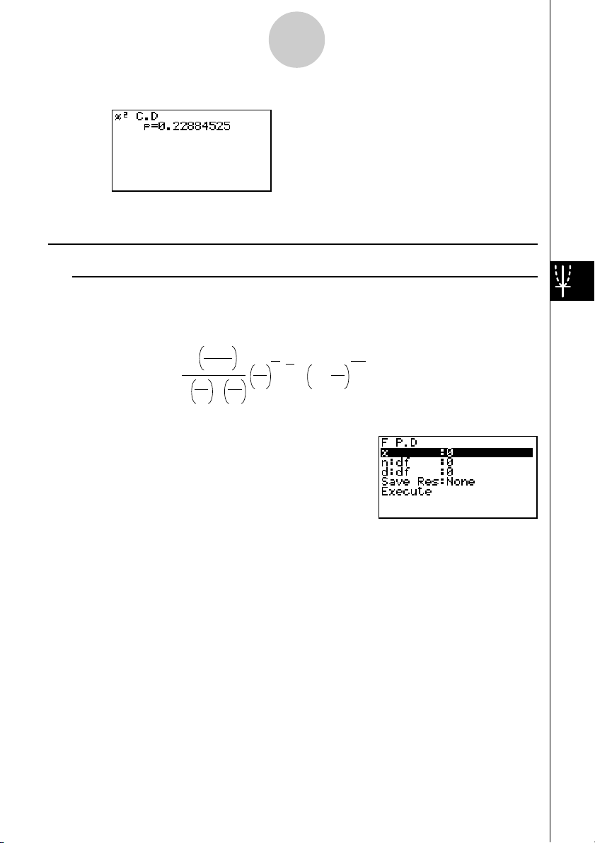
f
1-4-12
Distribution (DIST)
Calculation Result Output Example
p .................................. χ2 distribution probability
kk
k F Distribution
kk
uu
u F Probability Density
uu
F
probability density calculates the probability density function for the F distribution at a
specified x value.
n + d
Γ
(x) =
Perform the following key operations from the statistical data list.
5(DIST)
e(F)
b(P.D)
Data is specified using parameter specification. The following shows the meaning of each
item.
2
n
Γ
Γ
2
n
n
–1
2
2
n
d
x
d
2
1 +
nx
n + d
–
2
d
x .................................. data
n:df .............................. numerator degrees of freedom (positive integer)
d:df .............................. denominator degrees of freedom (positive integer)
Save Res..................... list for storage of calculation results (None or List 1 to 20)
Execute ....................... executes a calculation or draws a graph
After setting all the parameters, align the cursor with [Execute] and then press one of the
function keys shown below to perform the calculation or draw the graph.
• 1(CALC) ... Performs the calculation.
• 6(DRAW) ... Draws the graph.
20010101
20011101
Page 58

Calculation Result Output Example
p .................................. F probability density
1-4-13
Distribution (DIST)
# V-Window settings for graph drawing are set
automatically when the SET UP screen's
[Stat Wind] setting is [Auto]. Current V-
Window settings are used for graph drawing
when the [Stat Wind] setting is [Manual].
20010101
Page 59

1-4-14
Distribution (DIST)
uu
u F Distribution Probability
uu
F
distribution probability calculates the probability of F distribution data falling between two
specific values.
n + d
Γ
p =
Perform the following key operations from the statistical data list.
5(DIST)
e(F)
c(C.D)
Data is specified using parameter specification. The following shows the meaning of each
item.
Lower .......................... lower boundary
Upper .......................... upper boundary
2
n
Γ
Γ
2
n
b
n
2
∫
–1
2
1 +
x
a
n
d
d
2
nx
n + d
–
2
dx
d
a : lower boundary
b : upper boundary
n:df .............................. numerator degrees of freedom (positive integer)
d:df .............................. denominator degrees of freedom (positive integer)
Save Res..................... list for storage of calculation results (None or List 1 to 20)
Execute ....................... executes a calculation
After setting all the parameters, align the cursor with [Execute] and then press the function
key shown below to perform the calculation.
• 1(CALC) ... Performs the calculation.
# There is no graphing for F distribution
probability.
20010101
20011101
Page 60

Distribution (DIST)
Calculation Result Output Example
p .................................. F distribution probability
1-4-15
20010101
Page 61

f
1-4-16
Distribution (DIST)
kk
k Binomial Distribution
kk
uu
u Binomial Probability
uu
Binomial probability calculates a probability at a specified value for the discrete binomial
distribution with the specified number of trials and probability of success on each trial.
(x) = nC x px(1–p)
n – x
(x = 0, 1, ·······, n) p : success probability
(0 < p < 1)
n :number of trials
Perform the following key operations from the statistical data list.
5(DIST)
f(Binmal)
b(P.D)
The following shows the meaning of each item when data is specified using list specification.
Data ............................ data type
List .............................. list whose contents you want to use as specified data
(List 1 to 20)
Numtrial ....................... number of trials
p .................................. success probability (0 < p < 1)
Save Res..................... list for storage of calculation results (None or List 1 to 20)
Execute ....................... executes a calculation
The following shows the meaning of a parameter data specification item that is different from
list data specification.
x .................................. integer from 0 to n
After setting all the parameters, align the cursor with [Execute] and then press the function
key shown below to perform the calculation.
• 1(CALC) ... Performs the calculation.
# There is no graphing for binomial distribution.
20010101
20011101
Page 62

1-4-17
Distribution (DIST)
Calculation Result Output Example
p .................................. binomial probability
uu
uBinomial Cumulative Density
uu
Binomial cumulative density calculates a cumulative probability at a specified value for the
discrete binomial distribution with the specified number of trials and probability of success on
each trial.
Perform the following key operations from the statistical data list.
5 (DIST)
f (Binmal)
c (C.D)
The following shows the meaning of each item when data is specified using list specification.
Data ............................ data type
List .............................. list whose contents you want to use as specified data
(List 1 to 20)
Numtrial ....................... number of trials
p .................................. success probability (0 < p < 1)
Save Res..................... list for storage of calculation results (None or List 1 to 20)
Execute ....................... executes a calculation
The following shows the meaning of a parameter data specification item that is different from
list data specification.
x .................................. integer from 0 to n
20010101
20011101
Page 63

1-4-18
Distribution (DIST)
After setting all the parameters, align the cursor with [Execute] and then press the function
key shown below to perform the calculation.
• 1(CALC) ... Performs the calculation.
Calculation Result Output Example
p ......................................... probability of success
20010101
20011101
Page 64

1-4-19
Distribution (DIST)
kk
k Poisson Distribution
kk
uu
uPoisson Probability
uu
Poisson probability calculates a probability at a specified value for the discrete Poisson
distribution with the specified mean.
f(x) =
x!
(x = 0, 1, 2, ···)
µ
:mean (
µ
> 0)
µ
–
x
µ
e
Perform the following key operations from the statistical data list.
5(DIST)
g(Poissn)
b(P.D)
The following shows the meaning of each item when data is specified using list specification.
Data ............................ data type
List .............................. list whose contents you want to use as specified data
(List 1 to 20)
µ
.................................. mean (µ > 0)
Save Res..................... list for storage of calculation results (None or List 1 to 20)
Execute ....................... executes a calculation
The following shows the meaning of a parameter data specification item that is different from
list data specification.
x .................................. ( x
> 0)
After setting all the parameters, align the cursor with [Execute] and then press the function
key shown below to perform the calculation.
• 1(CALC) ... Performs the calculation.
Calculation Result Output Example
p .................................. Poisson probability
# There is no graphing for Poisson distribution.
20010101
20011101
Page 65
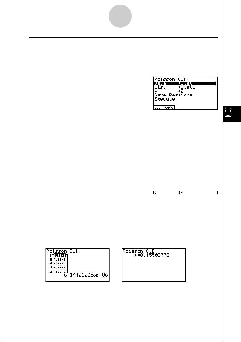
1-4-20
Distribution (DIST)
uu
u Poisson Cumulative Density
uu
Poisson cumulative density calculates a cumulative probability at specified value for the
discrete Poisson distribution with the specified mean.
Perform the following key operations from the statistical data list.
5(DIST)
g(Poissn)
c(C.D)
The following shows the meaning of each item when data is specified using list specification.
Data ............................ data type
List .............................. list whose contents you want to use as specified data
(List 1 to 20)
µ
.................................. mean (µ > 0)
Save Res..................... list for storage of calculation results (None or List 1 to 20)
Execute ....................... executes a caluculation
The following shows the meaning of a parameter data specification item that is different from
list data specification.
x .................................. ( x
> 0)
After setting all the parameters, align the cursor with [Execute] and then press the function
key shown below to perform the calculation.
• 1(CALC) ... Performs the calculation.
Calculation Result Output Example
p .................................. Poisson cumulative probability
20010101
20011101
Page 66

f
1-4-21
Distribution (DIST)
kk
k Geometric Distribution
kk
uu
uGeometric Probability
uu
Geometric probability calculates the probability at a specified value, and the number of the
trial on which the first success occurs, for the geometric distribution with a specified
probability of success.
(x) = p(1– p)
x – 1
(x = 1, 2, 3, ···)
Perform the following key operations from the statistical data list.
5(DIST)
h(Geo)
b(P.D)
The following shows the meaning of each item when data is specified using list specification.
Data ............................ data type
List .............................. list whose contents you want to use as specified data
(List 1 to 20)
p .................................. success probability (0 < p < 1)
Save Res..................... list for storage of calculation results (None or List 1 to 20)
Execute ....................... executes a calculation
The following shows the meaning of a parameter data specification item that is different from
list data specification.
x .................................. positive integer (x > 1)
After setting all the parameters, align the cursor with [Execute] and then press the function
key shown below to perform the calculation.
•1(CALC) ... Performs the calculation.
Calculation Result Output Example
p .................................. geometric probability
# There is no graphing for geometric distribu-
tion.
# Positive integer number is calculated whether
list data (Data:List) or
is specified.
20010101
20011101
x value (Data:var iable)
Page 67

1-4-22
Distribution (DIST)
uu
uGeometric Cumulative Density
uu
Geometric cumulative density calculates a cumulative probability at specified value, the
number of the trial on which the first success occurs, for the discrete geometric distribution
with the specified probability of success.
Perform the following key operations from the statistical data list.
5(DIST)
h(Geo)
c(C.D)
The following shows the meaning of each item when data is specified using list specification.
Data ............................ data type
List .............................. list whose contents you want to use as specified data
(List 1 to 20)
p .................................. success probability (0 < p < 1)
Save Res..................... list for storage of calculation results (None or List 1 to 20)
Execute ....................... executes a calculation
The following shows the meaning of a parameter data specification item that is different from
list data specification.
x .................................. positive integer (x > 1)
After setting all the parameters, align the cursor with [Execute] and then press the function
key shown below to perform the calculation.
• 1(CALC) ... Performs the calculation.
Calculation Result Output Example
p .................................. geometric cumulative probability
# Positive integer number is calculated whether
list data (Data:List) or
is specified.
x value (Data:variable)
20010101
20011101
 Loading...