

Page 1
Page 2

Quantity One
®
User Guide for Version 4.4
Windows and Macintosh
P/N 4000126-14 RevA
Page 3
Quantity One User Guide
¡
¢ ¢
¢ ¢ ¢
¢ ¢
¢
¢
¡
¢
¢
¢
¢
¢ ¢ ¡
¢
¢ ¢
ii
Page 4

Table of Contents
1. Introduction ........................................................................ 1-1
1.1. Overview of Quantity One .............................................................................. 1-1
1.2. Digital Data and Signal Intensity .................................................................... 1-2
1.3. Gel Quality ......................................................................................... ...... ....... 1-3
1.4. Quantity One Workflow ................................................................................. 1-4
1.5. Computer Requirements .................................. ............................................. .. 1-5
1.6. Installation ...................................................................................................... 1-7
1.7. Hardware Security Key (HSK) ....................................................................... 1-8
1.8. Starting the Program ..................................................................................... 1-10
1.9. Software License .......................................................................................... 1-11
1.10. Downloading from the Internet .................................................................. 1-14
1.11. Quantity One Basic ..................................................................................... 1-15
1.12. Contacting Bio-Rad .................................................................................... 1-16
2. General Operation .............................................................. 2-1
2.1. Menus and Toolbars ....................................................................................... 2-1
2.2. File Commands ............................................................................................... 2-6
2.3. Imaging Device Acquisition Windows ......................................................... 2-14
2.4. Exit ................................................................................................................ 2-15
2.5. Preferences .................................................................................................... 2-15
2.6. User Settings ............................................................................................ ..... 2-23
3 Viewing and Editing Images ............................................. 3-1
3.1. Magnifying and Positioning Tools ................................................................. 3-1
3.2. Density Tools .................................................................................................. 3-5
3.3. Showing and Hiding Overlays ............................... ..... ...... .............................. 3-6
3.4. Multi-Channel Viewer .................................................................................... 3-7
iii
Page 5

Quantity One User Guide
3.5. 3D Viewer ..................................................................................................... 3-10
3.6. Image Stack Tool .......................................................................................... 3-12
3.7. Colors ............................................................................................................ 3-14
3.8. Transform ...................................................................................................... 3-17
3.9. Resizing and Reorienting Images ................................................................. 3-23
3.10. Whole-Image Background Subtraction ....................................................... 3-29
3.11. Filtering Images .......................................................................................... 3-33
3.12. Invert Data ................................................................................................... 3-39
3.13. Text Overlays ................................... ............................................. ...... ........ 3-39
3.14. Erasing All Analysis from an Image ........................................................... 3-42
3.15. Sort and Recalculate .................................................................................... 3-42
3.16. Automation Manager .................................................................................. 3-42
4. Lanes .................................................................................. 4-1
4.1. Defining Lanes ................................................................................................ 4-1
4.2. Lane-Based Background Subtraction .............................................................. 4-9
4.3. Compare Lanes ............................................................................................. 4-13
4.4. Lane-based Arrays ........................................................................................ 4-16
5. Bands .................................................................................. 5-1
5.1. How Bands Are Identified and Quantified ..................................................... 5-2
5.2. Band Detection ................................................................................................ 5-3
5.3. Identifying and Editing Individual Bands ..................................................... 5-10
5.4. Plotting Traces of Bands ............................................................................... 5-12
5.5. Band Attributes ............................................................................................. 5-13
5.6. Band Information .......................................................................................... 5-16
5.7. Gauss-Modeling Bands ............................................................. .................... 5-18
5.8. Irregularly Shaped Bands in Lanes ............................................................... 5-21
6. Standards and Band Matching ...................................... ... 6-1
6.1. Standards ......................................................................................................... 6-1
6.2. Band Matching .............................................................................................. 6-13
iv
Page 6

Contents
6.3. Quantity Standards ........................................................................................ 6-24
7. Volume Tools ..................................................................... 7-1
7.1. Creating a Volume .......................................................................................... 7-1
7.2. Moving, Copying, and Deleting Volumes ...................................................... 7-6
7.3. Volume Standards ........................................................................................... 7-7
7.4. Volume Background Subtraction ................................................................... 7-8
7.5. Volume Arrays .............................................................................................. 7-11
8. Colony Counting ................................................................ 8-1
8.1. Defining the Counting Region ........................................................................ 8-2
8.2. Counting the Colonies .................................................................................... 8-3
8.3. Displaying the Results .................................................................................... 8-4
8.4. Making and Erasing Individual Colonies ....................................................... 8-5
8.5. Using the Histogram to Distinguish Colonies ................................................ 8-6
8.6. Ignoring a Region of the Dish ........................................................................ 8-8
8.7. Saving/Resetting the Count ............................................................................ 8-9
8.8. Saving to a Spreadsheet ................................................................................ 8-10
9. Differential Display and VNTRs ........................................ 9-1
9.1. Differential Display ........................................................................................ 9-1
9.2. Variable Number Tandem Repeats ................................................................. 9-3
10. Reports ............................................................................. 10-1
10.1. Report Window ........................................................................................... 10-1
10.2. Lane and Match Reports ....................................................... ..... ................. 10-5
10.3. Band Types Report ..................................................................................... 10-6
10.4. 1-D Analysis Report ................................................................................... 10-8
10.5. Similarity Comparison Reports .................................................................. 10-9
10.6. Volume Analysis Report ........................................................................... 10-20
10.7. Volume Regression Curve ........................................................................ 10-23
10.8. VNTR Report ............................................................................................ 10-25
v
Page 7

Quantity One User Guide
11. Printing and Exporting .................................................... 11-1
11.1. Print Image and Print Actual Size ............................................................... 11-1
11.2. Page Setup ................................................................................................... 11-1
11.3. Image Report ............................................................................................... 11-2
11.4. Video Print ........................................................ ..... ...... ............................... 11-3
11.5. Export to TIFF Image ................................................................................. 11-4
Appendix A.
Gel Doc 2000 ............................................................................. A-1
Appendix B.
ChemiDoc .................................................................................. B-1
Appendix C.
ChemiDoc XRS ......................................................................... C-1
Appendix D.
GS-700 Imaging Densitometer ................................................ D-1
Appendix E.
GS-710 Imaging Densitometer ............................... .... ..... ..... ... E-1
Appendix F.
GS-800 Imaging Densitometer ................................................ F-1
Appendix G.
Fluor-S MultiImager ......................... ..... ..... ............................... G-1
Appendix H.
Fluor-S MAX MultiImager ......................................................... H-1
vi
Page 8

Contents
Appendix I.
Personal Molecular Imager FX ................................................. I-1
Appendix J.
Molecular Imager FX Family (FX Pro, FX Pro Plus and Molecular
FX) .............................................................................................. J-1
Appendix K.
VersaDoc ................................................................................... K-1
Appendix L.
Cross-Platform File Exchange ................................................ L-1
Appendix M.
Other Features ......................................................................... M-1
vii
Page 9

Quantity One User Guide
viii
Page 10

Preface
1. About This Document
This user guide is designed to be used as a reference in your everyday use of Quantity
®
One
Software. It provides detailed information about the tools and commands of
Quantity One for the W indow s and Macinto sh platforms. Any platform dif feren ces in
procedures and commands are noted in the text.
This guide assumes that you have a working knowledge of your computer operating
system and its conventions, including how to use a mouse and standard menus and
commands, and how to open, save, and close files. For help with any of these
techniques, see the documentation that came with your computer.
This guide uses certain text conventions to describe specific commands and
functions.
Example Indicates
File > Open Choosing the Open command under the File menu.
Dragging Positioning t he cursor on an object and hol ding down
the left mouse button while you move the mouse.
Ctrl+s Holding down the Control key while typing the letter s.
Right-click/
Left-click/
Double-click
Some of the illustrations of menus and dialog boxes found in this manual are taken
from the Windows version of the software, and some are taken from the Macintosh
version. Both versions of a menu or dialog box will be shown only when there is a
significant difference between the two.
Clicking the right mouse button/
Clicking the left mouse button/
Clicking the left mouse button twice.
ix
Page 11

Quantity One User Guide
2. Bio-Rad Listens
The staff at Bio-Rad are receptive to your suggestions. Many of the new features and
enhancements in this version of Quantity One are a direct result of conversations with
our customers. Please let us know what you would like to see in the next version of
Quantity One by faxing, calling, or e-mailing our Technical Services staff. You can
also use Solobug (installed with Quantity One) to make software feature requests.
x
Page 12

1. Introduction
1.1 Overview of Quantity One
Quantity One is a powerful, flexible software package for imaging and analyzing 1-D
electrophoresis gels, dot blots, arrays, and colonies.
The software is supported on Windows and Macintosh operating systems and has a
graphical interface with standard pull-down menus, toolbars, and keyboard
commands.
Quantity One can image and analyze a wide variety of biological data, including
radioactive, chemiluminescent, fluorescent, and color-stained samples acquired from
densitometers, phosphor imagers, fluorescent imagers, and gel documentation
systems.
An image of a sample is captured using the controls in the imaging device window
and displayed on your computer monitor. Image processing and analysis operations
are performed using commands from the menus and toolbars.
Images can be magnified, annotated, rotated, and resized. They can be printed using
standard and video printers.
All data in the image can be quickly and accurately quantitated using the Volume
tools.
The lane-based functions can be used to determine molecular weights, isoelectric
points, VNTRs, presence/absence and up/down regulation of bands , and other values .
The software can measure total and average quantities, determine relative and actual
amounts of protein, and count colonies in a Petri dish.
The software can cope with distortions in the shape of lanes and bands. Lanes can be
adjusted along their lengths to compensate for any curvature or smiling of gels.
Image files can be shared among all The Discovery Series™ software. Images can
also be easily converted into TIFF format for compatibility with other Macintosh and
Windows applications.
1-1
Page 13
Quantity One User Guide
1.2 Digital Data and Signal Intensity
The Bio-Rad imaging devices supported by Quantity One are light and/or radiation
detectors that convert signals from biological samples into digital data. Quantity One
then displays the digital data on your computer screen, in the form of gray scale or
color images.
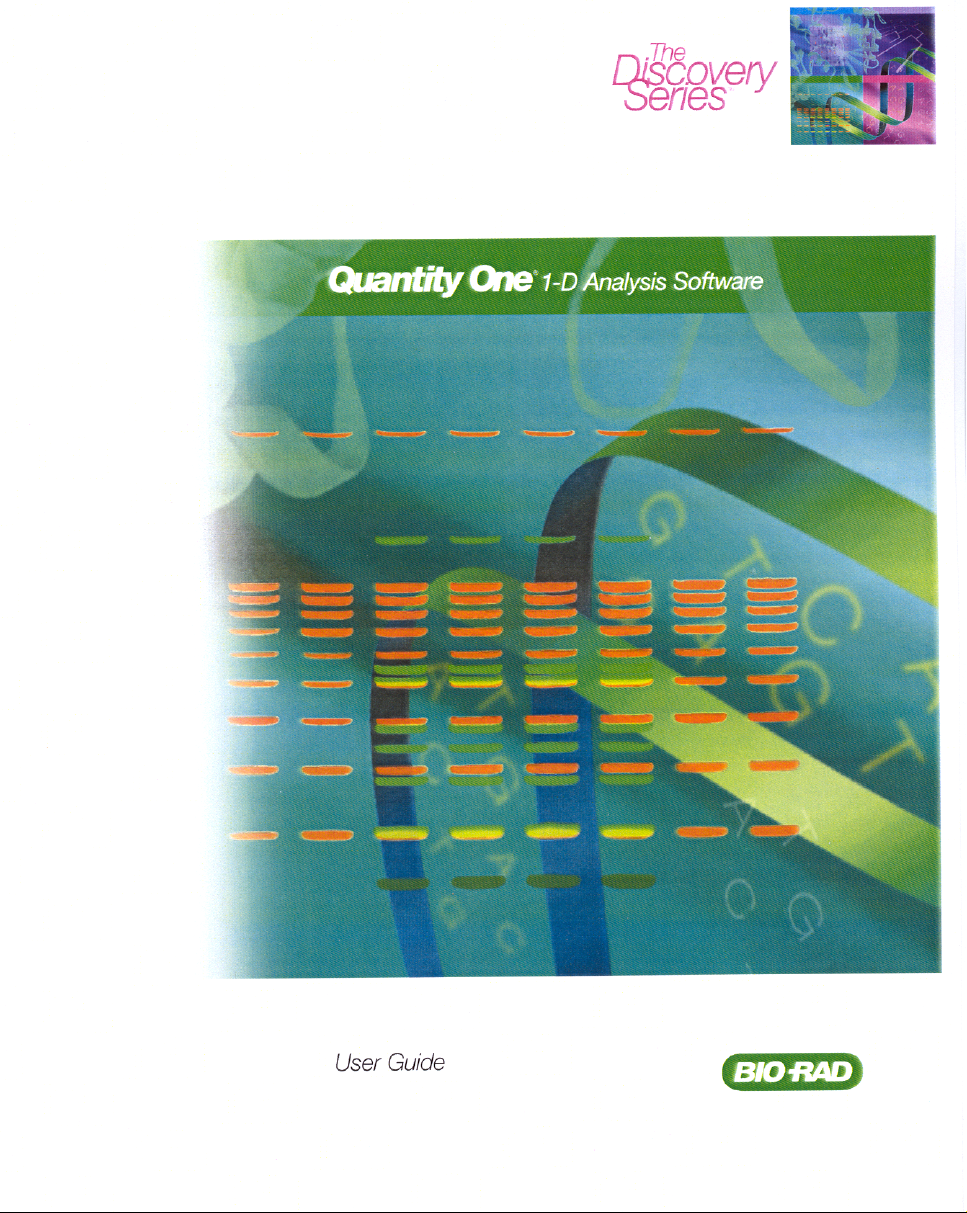
A data object as displayed on the computer is composed of tiny individual screen
pixels. Each pixel ha s an X an d Y coo rdinate, an d a valu e Z. Th e X and Y c oordi nates
are the pixel’s horizontal and vertical positions on the image, and the Z value is the
signal intensity of the pixel.
Signal intensity of a single pixel
Intensity
3-D View
2-D View
Fig. 1-1. Representation of the pixels in two digitally imaged bands in a gel.
For a data object to be visible and quantifiable, the intensity of its clustered pixels
must be higher than the intensity of the pixels that make up the background of the
image. The total intensity of a data object is the sum of the intensities of all the pixels
that make up the object. The mean intensity of a data object is the total intensity
divided by the number of pixels in the object.
The units of signal intensity are Optical Density (O.D.) in the case of the GS-700™
imaging densitometer, GS-710™ calibrated imaging densitometer, and GS-800™
calibrated densitometer, the Gel Doc™ system, ChemiDoc™ system, ChemiDoc
XRS™ system with a white light source, or the Fluor-S™ MultiImager system,
Fluor-S™ MAX MultiImager system, Fluor-S™ MAX2 MultiImager sy stem and
VersaDoc ™ imaging systems with white light illumination. Sig nal intensity is
expressed in counts when using the Personal Molecular Imager™ system or the
Molecular Imager FX™ system, Molecular Imager FX Pro™ fluorescent imager,
1-2
Page 14

Chapter 1. Introduction
Molecular Imager FX Pro Plus™ multiimager system, or in the case of the Gel Doc,
ChemiDoc, ChemiDoc XRS, Fluor -S, Fluor- S MAX, or VersaDoc when using the UV
light source.
1.3 Gel Quality
Quantity One is very tolerant of an assortment of electrophoretic artifacts. Lanes do
not have to be perfectly straight or parallel. Bands do not have to be perfectly
resolved.
However, for accurate lane-based quantitation, bands should be reasonably flat and
horizontal. Lane-based quantitation involves calculating the average intensity of
pixels across the band width and integrating over the band height. For the automatic
band finder to function optimally, bands should be well-resolved.
Dots that appear as halos, rings, or craters, or that are of unequal diameter, may be
incorrectly quantified using the automatic functions.
1-3
Page 15
Quantity One User Guide
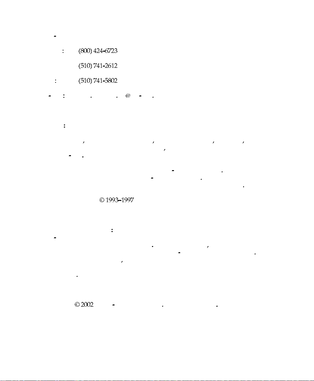
1.4 Quantity One Workflow
The following steps are involved in using Quantity One.
Acquire Image
Optimize Image
Lane and Band Analysis Volume Analysis Colony Counting
Report Results
Fig. 1-2. Quantity One workflow.
1.4.a Acquire Image
Before you can use Quantity One to analyze a biological image, you need to capture
the image and save it as an image file. This may be done with one of the several BioRad imaging instruments supported by this software: the Molecular Imager FX and
Personal Molecular Imager systems; the GS-700, GS-710, and GS-800 Imaging
Densitometers; the Gel Doc, ChemiDoc, and ChemiDoc XRS gel documentation
systems; the Fluor-S and Fluor-S MAX MultiImagers; and the VersaDoc.
The resulting images can be stored in files on a computer hard disk, network file
server, or removable disks.
1.4.b Optimize Image
Once you have acquired an image of your sample, you may need to reduce noise or
background density in the image. Quantity One has a variety of functions to minimize
image background while maintaining data integrity.
1-4
Page 16

Chapter 1. Introduction
1.4.c Analyze Image
Once a “clean” image is available, you can use Quantity One to gather and analyze
your biological data. In the case of 1-D gels, the software has tools for identifying
lanes and defining, quantifying, and calculating the values of bands. Volume tools
allow you to easily measure and compare the quantities of bands, spots, or arrays. The
colony counting controls allow you to count the number of colonies in a Petri dish, as
well as perform batch analysis.
Qualitative and quantitative data can be displayed in tabular and graphical formats.
1.4.d Report Results
When your analysis is complete, you can print your results in the form of simple
images, images with overlays, reports, tables, and graphs. You can export your
images and data to other applications for further analysis.
1.5 Computer Requirements
This software is supporte d on Windows 98, XP, NT 4.0, and 2000, or on a Macintosh
PowerPC.
The computer memory requirements are mainly determined by the file size of the
images you will scan and analyze. High-resolution image files can be very large. For
this reason, we recommend that you archive images on a network file server or highcapacity removable disk.
PC
The following is the recommended system configuration for installing and running
on a PC:
Operating system: Windows 98 SE
Windows NT 4.0 with service pack 6
Windows 2000
Windows XP
Processor: Pentium ≥ 333 MHz
1-5
Page 17

Quantity One User Guide
RAM: ≥ 128 MB or better for Gel Doc, ChemiDoc, ChemiDoc
XRS, and VersaDoc systems.
≥ 256 MB or better for Molecular Imager FX systems,
Personal FX system, and GS-800 densitometer.
Hard disk space: ≥ 3 GB
Monitor: 17" monitor, 1024 x 768 resolution (absolutely required),
True color.
SCSI: Required for all Bio-Rad imaging devices except the Gel
Doc, ChemiDoc, ChemiDoc XRS, and VersaDoc systems.
Adaptec SCSI card recommended.
Printer: Optional.
Macintosh
The following is the recommended system configuration for installing and running
on a Macintosh:
Operating system: System 9.0 or higher, excluding Mac OS X.
Processor/Model: PowerPC G3 processor or better.
RAM: ≥ 256 MB for all Bio-Rad imaging systems.
Hard disk space: ≥ 3 GB
Monitor: 17" monitor, 1024 x 768 resolution (absolutely required),
Millions of colors.
SCSI: Required for all Bio-Rad imaging devices except the Gel
Doc, ChemiDoc, ChemiDoc XRS, and VersaDoc systems.
Adaptec SCSI card recommended.
Printer: Optional.
Note: The default amount of memor y ass i gn ed to th is program on the Macintosh is 1 28
MB. If the total RAM in your Macintosh is 128 MB or less, you should reduce
the amount of memory assigned to the program to 10 MB
RAM. With the application icon selected, go to File > Get Info in your Finder to
1-6
less than your total
Page 18

Chapter 1. Introduction
reduce the memory requirements for the application. See your Macintosh
computer documentation for details.
1.6 Installation
1.6.a Windows
Note: Windows NT and 2000 users: You must be a member of the Administrators
group to install The Discovery Series software. After installation, members of the
Users group must have “write” access to The Discovery Series folder to use the
software.
Insert The Discovery Series CD-ROM into your computer. The installer will start
automatically. (If the CD does not auto-start, use Windows Explorer to open the root
directory on the CD-ROM and double-click on the Setup.exe file.)
The installer program will guide you through the installation. The installer will create
a default directory under Program Files on your computer called Bio-Rad\The
Discovery Series (you can select your own directory if you wish). The application
program will be placed in the Bin folder inside The Discovery Series folder.
Additional directories for storing user profiles and sample images will also be created
The installer will place an application icon on your d esktop and cre ate a fold er named
The Discovery Series under Programs on your Windows Start menu.
After installation, you must reboot your computer before using an imaging device.
1.6.b Macintosh
Insert The Discovery Series CD-ROM into your Macintosh. The TDS-Mac folder
will open on your desktop, displaying the installers for The Discovery Series
applications. Double-click on the installer for your application.
1-7
Page 19
Quantity One User Guide
Fig. 1-3. Installation program icon (Macintosh).
The installer will guide you through a series of screens. The installer will create a
folder on your hard drive that contains the main application and associated sample
images (you can select a different folder if you wish). The installation will also create
a folder called The Discovery Series in the Preferences folder in your System folder;
this contains the Help file and various system files.
Once installation is complete, the folder containing the application icon will appear
open on your desktop.
1.7 Hardware Security Key (HSK)
Note: Initial installation of a network server does require the Hardware Security Key
included in the software package. Installation of an additional Network Client
User to a Network License Server System does not require an HSK. Please refer
to the Network License Installation Guide that ships with Network Licenses .
The Discovery Series software is password-protected using a Hardware Security Key
(HSK), which is included in your software package. You must attach the Hardware
Security Key to your computer before you can run the software.
1.7.a Windows
Fig. 1-4. PC Hardware Security Key
1-8
Page 20
Chapter 1. Introduction
Before proceeding, please turn off your computer.
The HSK attaches to the parallel port on the back of your PC. If a printer cable is
attached to this port, turn off the printer and disconnect it. Af ter yo u have attached the
HSK, you can attach the printer cable to the key itself and restart your computer and
printer.
Note: Some parallel port devices such as zip drives may be incompatib le with HSKs.
Please check with your peripherals vendor.
The code for the PC hardware security key is EYYCY. This is printed on the key
itself.
You will also need to install the system driver that allows the computer to recognize
the HSK.
Note: Windows NT and 2000 users must be in the local administrator group to install
the HSK driver.
To install the driver, open the Windows Start menu and select Programs > The
Discovery Series. Select Install HASP Hardware Security Key Driver to begin
installation.
Note: Windows 98 users mus t reboot th eir computer after in stalling t he HSK. W ind ows
XP, NT and 2000 users do not have to reboot.
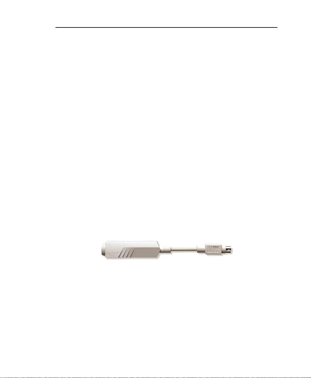
1.7.b Macintosh
Fig. 1-5. Macintosh Hardware Security Key
Before proceeding, please turn off your Macintosh.
The Macintosh HSK must be inserted in the Apple Desktop Bus (ADB) path. The
ADB port is located on the back of your Macintosh.
1-9
Page 21
Quantity One User Guide
Fig. 1-6. Apple Desktop Bus icon on back of Macintosh.
The HSK can be inserted at any point in the ADB path—between the computer and
the keyboard, between the keyboard and the mouse, between the keyboard and the
monitor, etc. After you have attached the HSK, you can restart your computer.
The code for the Macintosh HSK is QCDIY. This code is printed on the key itself .
Note: If your Macintosh does not have an ADB, you may use an ADB-USB converter.
1.8 Starting the Program
The Hardware Security Key must be attached to the co mputer b efore yo u can st art the
software (unless you are using a network license).
1.8.a Windows
The installation program creates an application icon on your desktop. To start the
program, double-click on this icon.
Fig. 1-7. Application i c on.
You can also start the program from the Windows Start menu. Click on the Start
button, select Programs, select The Discovery Series, and select the application name.
1-10
Page 22
Chapter 1. Introduction
1.8.b Macintosh
After installation, the main application folder will be open on your desktop. To start
the program, double-click on the application icon shortcut inside the folder. You can
move this shortcut icon to your desktop.
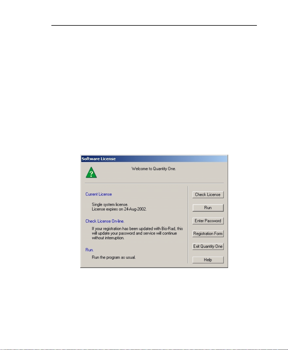
1.9 Software License
When the software opens for the first time, you will see a Software License screen that
shows the current status of your software license.
With a new HSK or network license, you receive a 30-day temporary license (“Your
license will expire on _______”). The temporary license is designed to give you time
to purchase the software, if you have not already done so.
Fig. 1-8. Temporary license screen.
During the 30-day period, the Software License screen will appear every time you
open the software. To use the software during this period, click on the Run button.
1-11
Page 23
Quantity One User Guide
Network license holders can click on the Check License button at any time during th e
30-day period to activate their full network license. (If your network license is not
activated when you click on Check License, notify your network administrator.)
HSK users have 30 day s to p urchase the sof tware and obt ain a pu rchase o rder nu mber
and software serial number from Bio-Rad. When you have this information, click on
the Check License or Registration Form button in the Software License screen to
register your software.
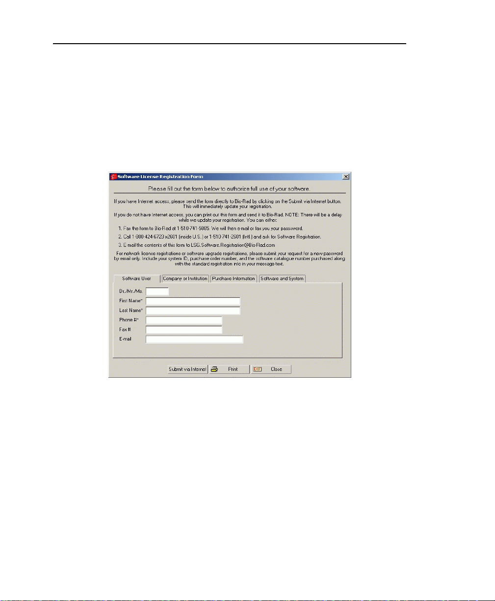
Fig. 1-9. Software License Registration Fo rm.
Fill out the information in the Software License Registration Form. Be sure to enter
your purchase order number and software serial number under the Purchase
Information tab when registering.
1.9.a Registering by Internet
If you have Internet access from your computer, click on the Submit via Internet
button to send the Software Registration Form directly to Bio-Ra d.
1-12
Page 24

Chapter 1. Introduction
Your information will be submitted, and a temporary password will be generated
automatically and sent back to your computer. Simply continue to run the application
as before.
Bio-Rad will confirm your purchase information and generate a permanent license .
After 2–3 days, click on Check License in the Software License screen again to
update to a permanent password. (The Software License screen will not appear
automatically after the temporary password has been generated; the software will
simply open normally. Go to the Help menu and select Register to open the Software
License screen.)
1.9.b Registering by Fax or E-mail
If you do not have Internet access, click on the Print button in the Software License
Registration Form and fax the form to Bio-Rad at the number listed on the form.
Alternatively , yo u can en ter the conten ts of the form into an e-mail and send it to BioRad at the address listed in the Registratio n Form.
Bio-Rad will contact you by fax or e-mail in 2–3 days with a full license.
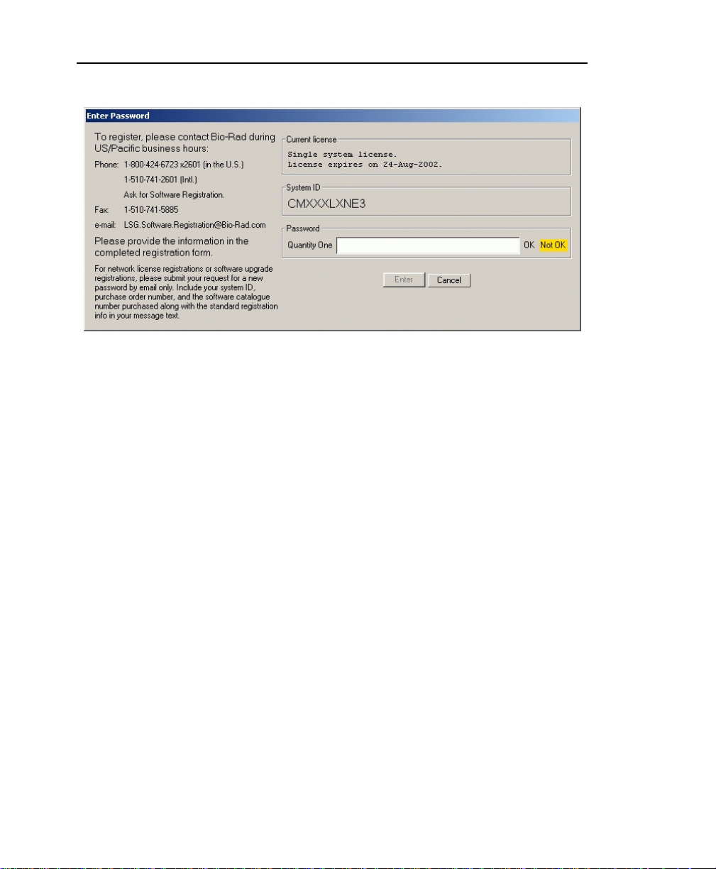
1.9.c Entering a Password
If you fax or e-mail your registration information, you will receive a password from
Bio-Rad. You must enter this password manually.
To enter your password, click on Enter Password in the Software License screen. If
you are not currently in the Software License screen, select Register from the Help
menu.
1-13
Page 25
Quantity One User Guide
Fig. 1-10. Enter Password screen.
In the Enter Password screen, type in your password in the field.
Once you have typed in the correct password, the OK light next to the password field
will change to green and the Enter button will activate. Click on Enter to run the
program.
1.10 Downloading from the Inte rnet
You can download a trial version of the so ft wa re f rom Bi o- Rad’s Web s i te. Go to Th e
Discovery Series download page at www.bio-rad.com/softwaredownloads and
select from the list of applications. Follow the instructions to download the installer
onto your computer, then run the installer.
After installation, double-click on the application icon to run the program. The
software will open and the Software License screen will be displayed.
Note: If you attempt to start the downloaded program and receive an “Unable to obtain
authorization” message, you will need a Hardware Security Key to run the
program. Contact Bio-Rad to obtain a key.
1-14
Page 26
Chapter 1. Introduction
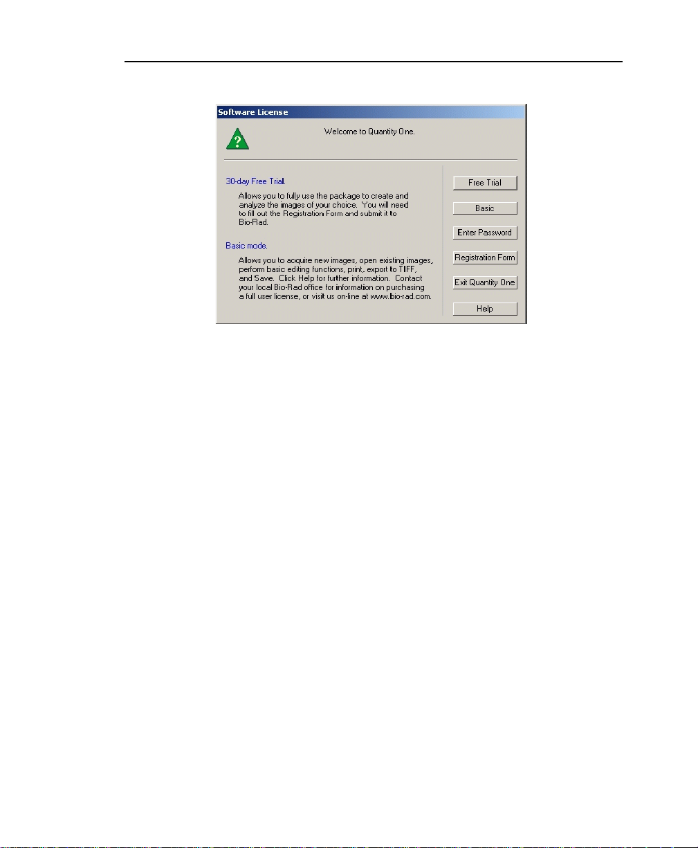
Fig. 1-11. Free Trial screen.
In the Software License screen, click on the Free Trial button. This will open the
Software License Registration Form. Enter the required information (you will not
have a purchase order number or software serial number, and can leave these fields
blank) and click on Submit V ia Internet.
A free trial password will be automatically downloaded to your computer. This
password will allow you to use the software for 30 days.
If you decide to purchase the software during that period, contact Bio-Rad to receive
a software package and a Hardware Security Key. You can then complete the
registration process as described in the previous sections.
1.11 Quantity One Basic
Quantity One can be run in Basic mode. Quantity One Basic does not require a
software license. The program can be i ns talled and used simultaneously on unlimit ed
numbers of computers. Quantity One Basic is a limited version of the flexible and
powerful Quantity One.
1-15
Page 27

Quantity One User Guide
The following functionality is active in Basic Mode: Image acquisition with Bio-Rad
imaging devices, Transform, Crop, Flip, Rotate, Text Tool, Volume Rectangle Tool,
Volume Circle Tool, Density Tools, Print, Export to TIFF, and Save.
1.12 Contacting Bio-Rad
Bio-Rad technical service hours are from 8:00 a.m. to 4:00 p.m., Pacific Standard
Time in the U.S.
Phone: 800-424-6723
510-741-2612
Fax: 510-741-5802
E-mail: LSG.TechServ.US@Bio-Rad.com
For software registration:
Phone: 800-424-6723 (in the U.S.)
+1-510-741-6996 (outside the U.S.)
1-16
Page 28

2. General Operation
This chapter describes the graphical interface of Quantity One, how to access the
various commands, how to open and s ave images , h ow to set pref erences , an d how to
perform other basic file commands.
2.1 Menus and Toolbars
2.1.a Menu Bar
Quantity One has a standard menu bar with pulldown m enus that co ntain all the m ajor
features and functions available in the software.
• File—Opening and saving fi le s, imagi ng device contro ls, pri nti ng , exporti ng .
• Edit—Preferences, other settings.
• View—Image magnification and viewing tools, tools for viewing image data.
• Image—Image transform, advanced crop, image processing and modification.
• Lane—Lane-finding tools.
• Band—Band-finding and band-modeling tools.
• Match—Tools for calculating molecular weights and other values from
standards, tools for comparing lanes and bands in lanes.
• Volume—Band quantity and array data tools.
• Analysis—Colony counting, Differential Display, VNTR analysis.
• Reports—Band and lane analysis reports, Phylogenetic Tree, Similarity Matrix.
• Window—Commands for arranging multiple image windows.
• Help—Quick Guides, on-line Help, software registration.
Below the menu bar is the main toolbar, containing some of the most common ly used
commands. Next to the main toolbar are the status boxes, which provide information
about cursor selection and toolbar buttons.
2-1
Page 29
Quantity One User Guide
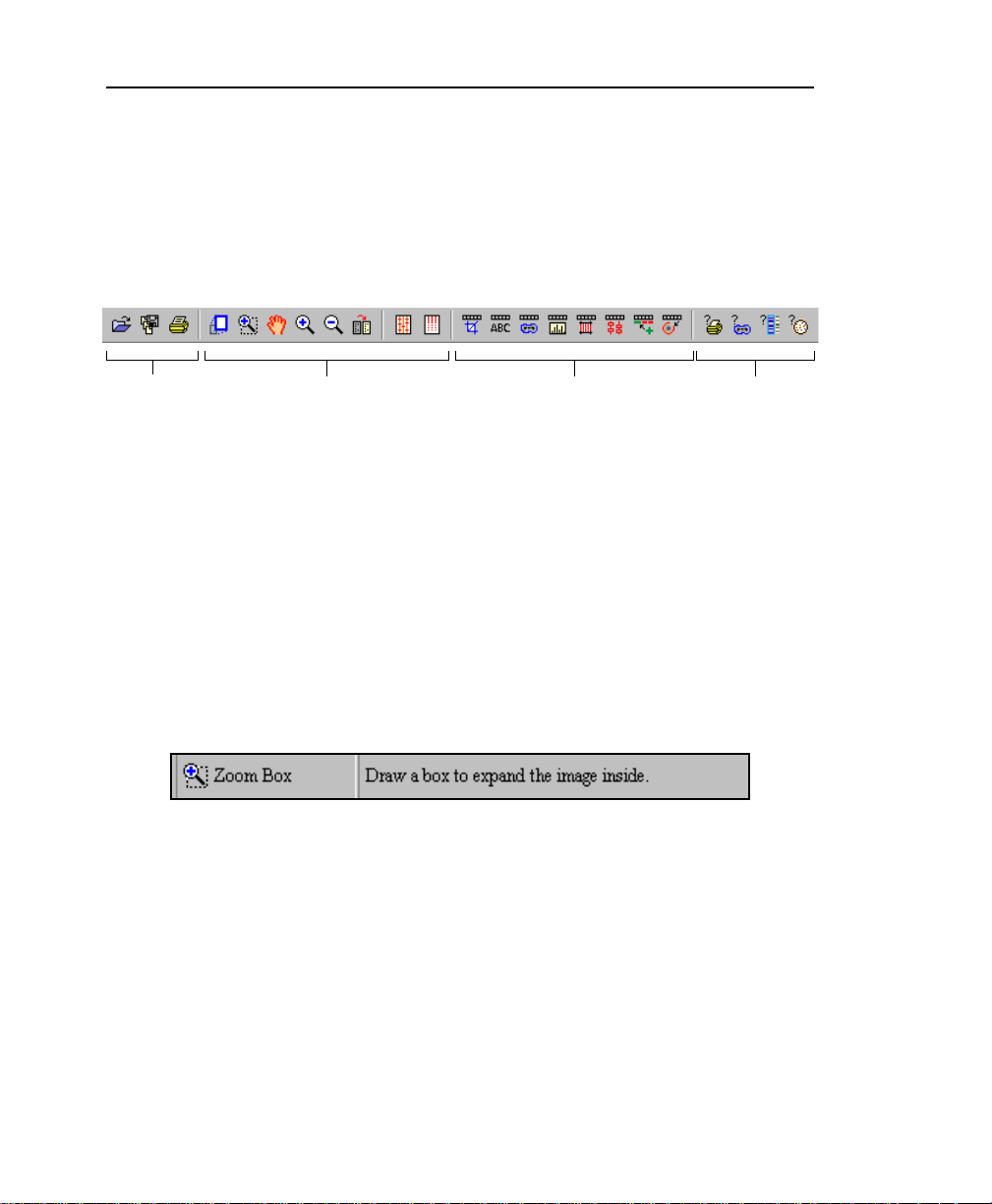
2.1.b Main Toolbar
The main toolbar appears below the menu. It includes buttons for the main file
commands (Open, Save, Print) and essential viewing tools (Zoom Box, Grab, etc.) ,
as well as buttons that open the secondary toolbars and the most u seful Quick Guid es
(Printing, Volumes, Molecular Weight, and Colony Counting).
File commands Viewing commands Toolbars Quick Guides
Fig. 2-1. Main toolbar.
Tool Help
If you hold the cursor over a toolbar icon, the name of the command will pop up
below the icon. This utility is called Tool Help. Tool Help appears on a time delay
basis that can be specified in the Preferences dialog box (see section
Preferences). You can also specify how long the Tool Help will remain displayed.
2.5,
2.1.c Status Boxes
There are two status boxes, which appear to the right of the main toolbar.
Fig. 2-2. Status boxes.
The first box displays any function that is assigned to the mouse. If you select a
command such as Zoom Box , the name and icon of that command will appear in this
status box and remain there until another mouse function is selected or the mouse is
deassigned.
The second status box is designed to supplement Tool Help (see above). It provides
additional information about the toolbar buttons. If you hold your cursor over a
2-2
Page 30
Chapter 2. General Information
button, a short expl anation about t hat command w ill be disp layed in thi s second statu s
box.
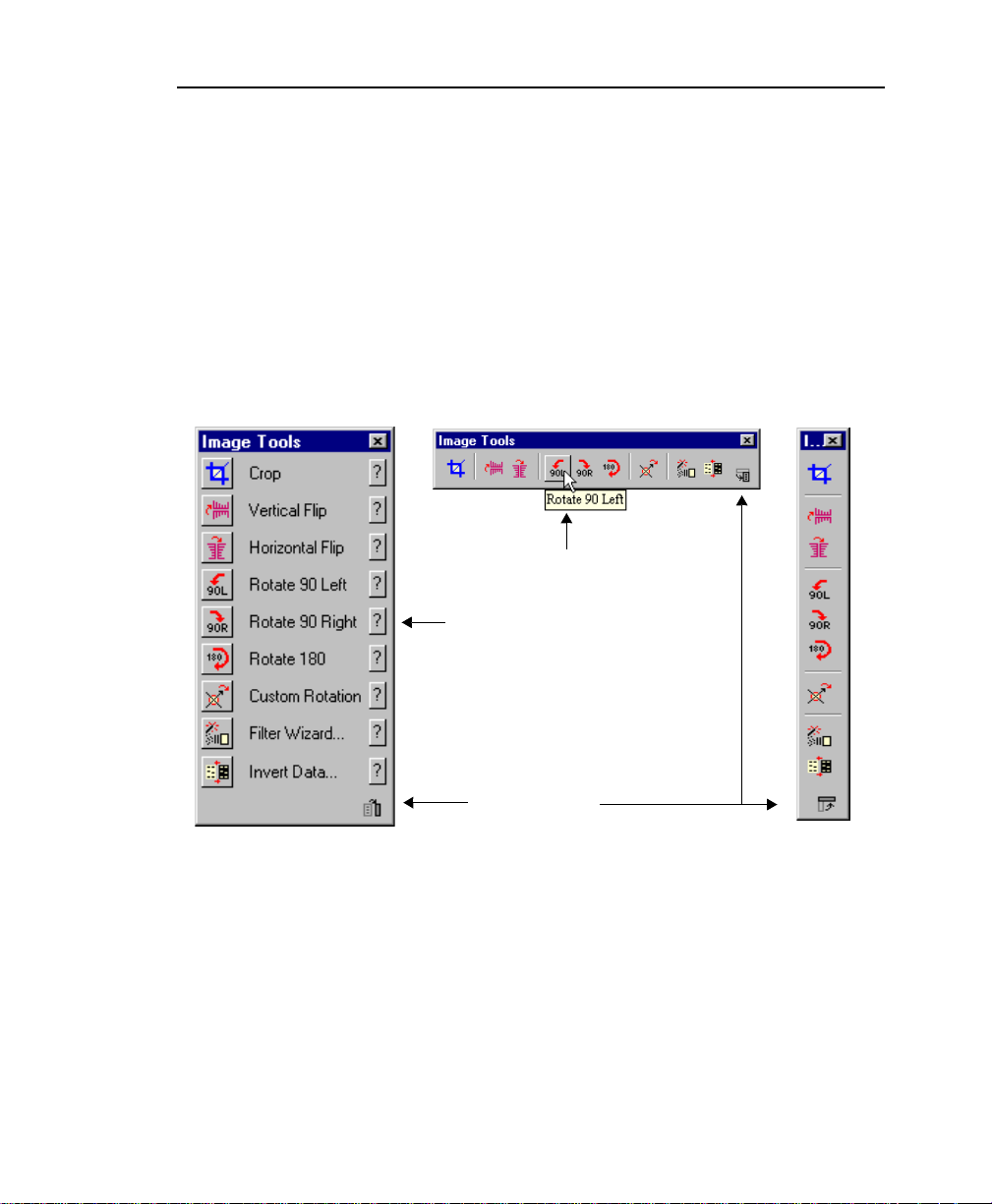
2.1.d Secondary Toolbars
Secondary toolbars contain groups of related functions. You can open these toolbars
from the main toolbar or from the View > Toolbars submenu.
The secondary toolbars can be toggled between vertical, horizontal, and expanded
formats by clicking on the resize button on the toolbar itself.
Expanded format
Fig. 2-3. Secondary toolbar formats and features.
Horizontal format Vertical format
Hold cursor over icon
to reveal the “tool tip”
Click on question marks
for on-line help
Click on resize button
to toggle format
The expanded toolbar format shows the name of each of the commands. Click on the
? icon next to the name to display on-line Help for that command.
2-3
Page 31
Quantity One User Guide
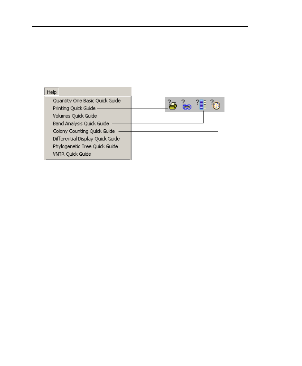
2.1.e Quick Guides
The Quick Guides are designed to guide you through the major applications of the
software. They are listed under the Help menu; four of these are also available on the
main toolbar.
Fig. 2-4. Quick Guides listed on Help menu and main toolbar.
The Quick Guides are similar in design to the secondary toolbars, but are applicationspecific. Each Quick Guide contains all of the functions for a particular application,
from opening the image to outputting data.
2-4
Page 32

Select Volumes
Quick Guide from
main toolbar
Commands are numbered
to indicate sequence for
preparing the image,
creating volumes, and
outputting data
Key commands
Chapter 2. General Information
Question marks
open on-line
Help
Toggle format
Fig. 2-5. Example of a Quick Guide: Volume s
In their expanded format, the Quick Guide commands are numbered as well as
named. The numbers provide a suggested order of operation; however, not every
command is required for every application.
As with the secondary toolbars, you can click on the ? next to the name of a function
to display the Help text.
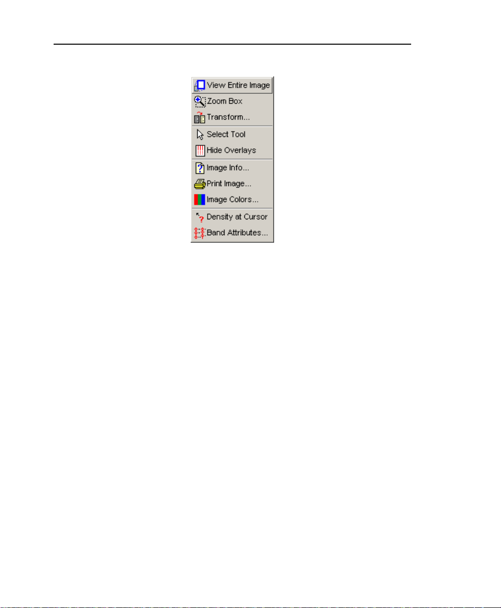
2.1.f Right-Click Context Menu
With an image open, right-click anywhere on the image to display a context menu of
common commands.
2-5
Page 33
Quantity One User Guide
Fig. 2-6. Selecting Zoom Box from the right-click context menu.
You can select commands from this menu as you would from a standard menu.
2.1.g Keyboard Commands
Many commands and functions can be performed using keyboard keys (e.g., press the
F1 key for View Entire Image; press Ctrl+S for Save). Select Keyboard Layout
from the Help menu to display a list of keys and key combinations and their
associated commands.
The pulldown menus also list the shortcut keys for the menu commands.
2.2 File Commands
The basic file commands and functions are located on the File menu.
2-6
Page 34

Chapter 2. General Information
Fig. 2-7. File menu.
2.2.a Opening Images
To open a saved image, select Open from the File menu or click on the Open button
on the main toolbar. This opens the standard Open dialog box for your operating
system.
2-7
Page 35

Quantity One User Guide
Macintosh version:
Windows version:
Fig. 2-8. Open dialog box.
In the dialog box, open a file by double-clicking on the file name. To open multiple
files, first select them using Ctrl-click or Shift-click key combinations, and then click
on the Open button.
An image created in the Windows version of Quantity One can be opened in the
Macintosh version, and visa versa. However, you must add a .1sc extension to your
Macintosh files to open them in Windows.
Note: This version of Quantity One will open any image created with an earlier version
of Quantity One.
2-8
Page 36

Chapter 2. General Information
You can also open images from other The Discovery Series software (PDQuest,
Diversity Database, DNACode).
The application comes with a selection of sample images. In Windows, these are
located in The Discovery Series/Sample Images/1D directory. On the Macintosh, they
are stored in the Sample Images folder in the Quantity One folder.
Opening TIFF Images
The Open command can also be used to import TIFF images created using other
software applications.
There are many types of TIFF formats that exist on the market. Not all are supported
by The Discovery Series. There are two broad categories of TIFF files that are
supported:
1. 8-bit Grayscale. Most scanners have an option between line art, full color, and
grayscale formats. Select grayscale for use with The Discovery Series software.
In a grayscale format, each pixel is assigned a value from 0 to 255, with each
value corresponding to a particular shade of gray.
2. 16-bit Grayscale. Bio-Rad’s Molecular Imager FX and Personal Molecular
Imager and Fluor-S, and VersaDoc imaging systems use 16-bit pixel values to
describe intensity of scale. Molecular Dynamics
bit pixel values. The Discovery Series understands these formats and can
interpret images from both Bio-Rad and Molecular Dynamics storage phosphor
systems.
™
and Fuji™ imagers also use 16-
Note: The program can import 8- and 16-bit TIFF images from both Maci ntosh and PC
platforms.
TIFF files that are not supported include:
1. 1-bit Line Art. This format is generally used for scanning text for optical
character recognition or line drawings. Each pixel in an image is read as either
black or white. Because the software needs to read continuous gradations to
perform gel analysis, this on-off pixel format is not used.
2. 24 -bit Full Colo r or 256 Indexe d Color. These formats are frequently used for
retouching photographs and are currently unsupported in The Discovery Series,
2-9
Page 37

Quantity One User Guide
although most scanners that are capable of producing 24-bit and indexed color
images will be able to produce grayscale scans as well.
3. Compressed Files. The software does not read compressed TIFF images. Since
most programs offer compression as a selectable option, files intended for
compatibility with The Discovery Series should be formatted with the
compression option turned off.
2.2.b Saving Images
To save a new image or an old image with changes, select Save from the File menu.
In Windows, new images will be given a .1sc extension when they are first saved.
Save As can be used to save a new image, rename an old image, or save a copy of an
image to a different directory. The standard Save As dialog box for your operating
system will open.
T o save all op en imag es, select Save All from the File menu or cl i ck o n t he but to n on
the main toolbar.
2.2.c Closing Images
To close an image, select Close from the File menu. To close all open images, select
Close All. You will be prompted to save any changes before closing.
2.2.d Revert to Saved
To reload the last saved version of an image, select Revert to Saved from the File
menu. Because any changes you made since last saving the file will be lost, you will
be prompted to confirm the command.
2.2.e Image Info
Image Info on t he File menu opens a dialog box containing general information
about the selected image, including scan date, scan area, number of pixels in the
image, data range, and the size of the file. Type any description or comments about
the image in the Description field.
2-10
Page 38

Chapter 2. General Information
Fig. 2-9. Image Info box.
History lists the changes made to the image including the date. If you have Security
Mode active, the name of the user who made the change is also listed (See Section
2.5, Preferences for information on Security Mode).
To print the file info, click on the Print button in the dialog box.
Changing the Image Dimensions
You can change the dimensions of certain images using the Image Info dialog box.
This feature is only available for images captured by a camera or imported TIFF
images in which the dimensions are not already specified.
2-11
Page 39

Quantity One User Guide
For these types of images, the Image Info dialog box will include fields for changing
the image dimensions.
Fields for changing
the image dimensions
Fig. 2-10. Image Info dialog box with fields for changing the image dimensions.
Enter the new image dimensions (in millimeters) in the appropriate fields. Note that
the pixel size in the image (in micrometers) will change to retain the same number of
pixels in the image.
2.2.f Reduce File Size
High-resolution image files can be very large, which can lead to problems with
opening and saving. To reduce the file size of an image, you can reduce the image
resolution by reducing the number of pixels in the image. (You can also trim
unneeded parts of an image to reduce its memory size. See section
Images.)
2-12
3.9.a, Cropping
Page 40

Chapter 2. General Information
This function is comparable to scanning at a lower resolution, in that you are
increasing the size of the pixels in the image, thereby reducing the total number of
pixels and thus the file size.
Note: In most cases, reducing the resolution of an image will not affect quantitation. In
general, as long as the pixel size remains less than 10 percent of the size of the
objects in your image, changing the pixel size will not affect quantitation.
Select Reduce File Size from the File menu to open the Reduce File Size dialog box.
The dialog box lists the size of the pixels in the image (Pixel Size: X by Y microns),
the number of pixels in the image (Pixel Count: X by Y pixels), and the memory size
of the image.
Before:
Pixel size in the “x” dimension increased
After:
Pixel Count and Memory Size reduced
Fig. 2-11. Reduce File Size dialog box, before and after pixel size increase.
Lower the resolution by entering lower values in the Pixel Count fields or higher
values in th e Pixel Size fields (see the figure for an example).
2-13
Page 41

Quantity One User Guide
Note: Since with most 1-D gels you are more concerned with resolving bands in the
vertical direction than the horizontal direction, you may want to reduce the file
size by making rectangular pixels. That is, keep the pixel size in the “y”
dimension the same, while increasing the size in the “x” dimension.
When you are finished, click on the OK button.
A pop-up box will g ive you the op tion of red ucing the file size o f the di spla yed image
or making a copy of the image and then reducing the copy’s size.
Reducing the file size is an irreversible process. For that reason, we suggest that you
first experiment with a copy of the image. Then, when you are satisfied with the
reduced image, delete the original.
Fig. 2-12. Confirm Reduce File Size pop-up box.
2.3 Imaging Device Acquisition Windows
The File menu contains a list of Bio-Rad imaging devices supported by Quantity One.
These are:
1. Gel Doc
2. ChemiDoc
3. Ch emiDoc XRS
4. GS-700 Imaging Densitometer
2-14
Page 42

Chapter 2. General Information
5. GS-710 Imaging Densitometer
6. GS -800 Calibra ted Densitometer
7. Fluor-S MultiImager
8. Fluor-S MAX MultiImager
9. Fluor-S MAX2 MultiImager
10. VersaDoc
11. Personal Molecular Imager FX
12. Molecular Imager FX
T o op en the acqu isition window for an imaging device, select the nam e of that device
from the File menu.
See the individual chapters on the imaging devices for more details.
2.4 Exit
T o close Quantity One, select Exit from the File menu. You will be prompted to save
your changes to any open files.
2.5 Preferences
You can custo mize basic features of Quantity One—such as menu options, display
settings, and toolbars—using the Preferences dialog box. Select Preferences from the
Edit menu to open this dialog.
2-15
Page 43

Quantity One User Guide
Fig. 2-13. Preferences dialog box.
Click on the appropriate tab to access groups of related preferences. After you have
selected your preferences, click on OK to implement them.
2.5.a Misc.
Click on the Misc tab to access the following preferences.
Memory Allowance
To specify the amount of virtual memory allocated for the application at start-up,
enter a value (in megabytes) in the Memory Allowance field. The default value of
512 megabytes is recommended. If yo u receive a war ning mes sage that the amou nt of
virtual memory is set too high, you can enter a smaller value in this field. However,
this should be considered a temporary fix, and you should consider expanding your
hard drive.
Institute Name
Enter the name of your institution in this field.
2-16
Page 44

Chapter 2. General Information
Security Mode
Security Mode allows you to set up a list of users who can activate Quantity One
functions on the local machine. Security Mode allows you to track any changes made
to images. If Security Mode is active, select File>Image Info... to view the list of
changes to the file and who made the changes.
T o activate Security Mode, check the box labeled Security Mode. Once ch ecked, you
will be prompted for a new Security Mode password which will be required for
making changes, adding or removing users, or for disabling Security Mode.
With Security Mode active, a user must enter a user name and password to activate
Quantity One commands. Security Mode is machine specific, so any images residing
on a network or shared drive can be accessed from another machine that does not
have Security Mode active. Although changes made on other machines are recorded
in the Image info dialog, no user name appears. The same is also true for changes
made to images while Security Mode is inactive.
Auto Logout
To have Quantity One automatically log out the current user after a period of
inactivity, check the box labeled Auto Logout after and enter a number of minutes in
the field. After the time has expired, the user will have to log in again to resume using
Quantity One.
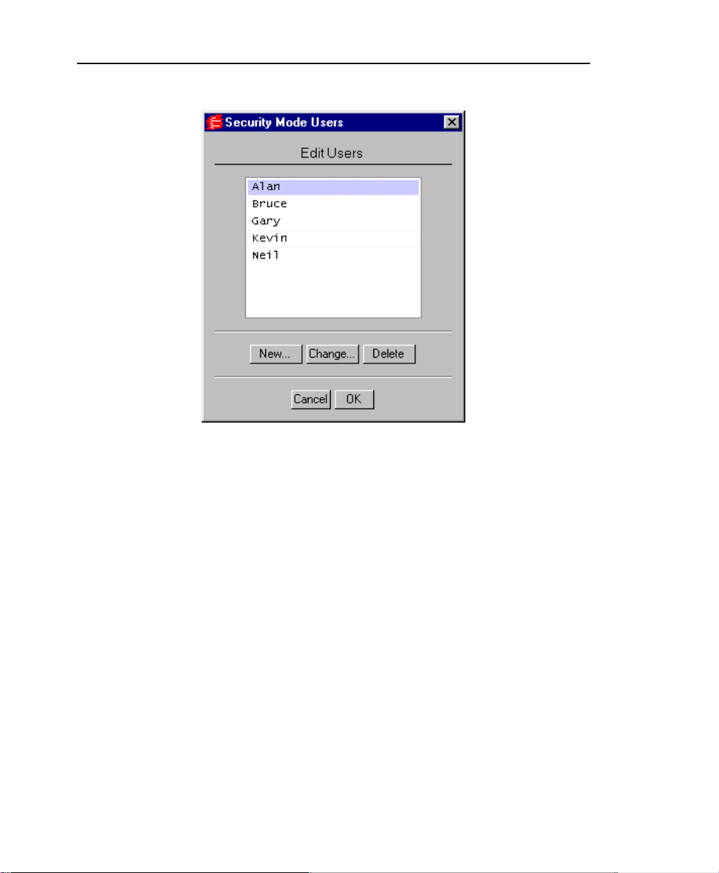
Adding and Removing Users
Once you activate Security Mode, you can add users to your list. Click Edit Users to
open the Security Mode Users dialog.
2-17
Page 45
Quantity One User Guide
Fig. 2-14. Security Mode Users Dialog
Click Add to add a new user. Enter a user name and password. To remove a user,
highlight the name in the list and click Remove. This permanently removes the user
from the list. However , any changes made by this user re main in the history secti on of
the Image Info dialog.
GLP/GMP Mode
The GLP/GMP Mode checkbox allows you to prevent changes to an image that
would change the raw image data. In GLP/GMP mode, the following commands and
submenus will be disabled:
• Reduce File Size (File menu)
• Subtract Background (Image menu)
• Custom Rotation (Image menu)
• Filter Wizard (Image menu)
• Filter List (Image menu)
2-18
Page 46

Chapter 2. General Information
• Invert Data (Image menu)
If you attempt to use any of these functions in GLP/GMP mode, you will receive a
message that the function is not available.
To set GLP/GMP mode, click on the checkbox. You will be prompted to enter the
Security Mode password.
To disable GLP/GMP mode, click on the checkbox to deselect it, then enter the
Security Mode password for confirmation.
Note: GLP/GMP mode is only available if Security Mode is active.
Use Custom Open Dialog
By default, Quantity One uses the standard Open dialog box for the operating syst em
you are using (Windows and Macintosh). Quantity One also has a customized Open
dialog box, which includes some navigational features that are specifically tailored to
The Discovery Series software. Select this checkbox to display this custom dialog
box.
Maximize Applic ation Window
In the Windows version, select the Maximize Application Window checkbox to
automatically maximize the application window when Quantity One first opens. If
this is unchecked, the menu and status bars will appear across the top of the screen
and any toolbars will appear “floating” on the screen.
Enable DOS Filename Parsing
If this checkbox is selected, for 8-character file names ending in two digits, the final
two digits are interpreted as version and exposure numbers. For example, the file
name IMAGE-11.1 sc would be p arsed as IMAG E
enable backwards compatibility for users with DOS image files. You should only
check this box if you are using these image files.
2-19
ver 1 xpo 1.1sc. This is designed to
Page 47

Quantity One User Guide
Enable UNIX Filename Parsing
This is similar to DOS file name parsing. Windows and Macintosh users are unlikely
to run into difficulties with UNIX parsing; therefore, this setting is checked by
default.
2.5.b Paths
Click on the Paths tab to access the following preference.
Temporary File Location
Temporary image files are normally stored in the TMP directory of your The
Discovery Series folder. The full path is listed in the field. To change the location of
your tempor ary files, click on Browse and select a new directory. To return to the
default TMP directory, click on the Default checkbox.
2.5.c Display
Click on the Display tab to access the following preferences.
Zoom %
Zoom % determines the percen tage by which an image zooms i n or out when yo u use
the Zoom In and Zoom Out functions. This percentage is based on the size of the
image.
Pan %
Pan % determines the percentage by which the image moves side to side or up and
down when you use the arrow keys . T his percen t age i s bas ed on the size of the image.
Jump Cursor on Alert (Windows only)
Select Jump Cursor on Alert to set the cursor to automatically jump to the OK
button in a pop-up dialog box.
2-20
Page 48

Chapter 2. General Information
Auto “Imitate Zoom”
When this checkbox is selected, the magnifying and image positioning commands
used in one window will be applied to all open windows. This is useful, for example,
if you want to compare the same band of group of bands in dif ferent gels ; magnify the
band(s) in one gel, and the same area will be magnified in all the other gel images.
Note that the images must be approximately the same size.
Band Style
Bands in your gel image can be marked with brackets that define the top and bottom
boundaries of the band, or they can be marked with a dash at the center of the band.
Indicate your preference by clicking on the Brackets or Lines button. (This setting
can be temporarily changed in the Band Attribu tes dialog box. However, all newly
opened images will use the preferences setting.)
2.5.d Toolbar
Click on the Toolbar tab to access the following preferences, which determine the
behavior and positioning of the secondary toolbars and Quick Guides.
Show Volumes Quick Guide
If this checkbox is selected, the Volumes Quick Guide will open automatically when
you open the program.
Align Quick Guide with Document
If this checkbox is selected, the Quick Guides will open flush with the edge of your
documents. Otherwise, they will appear flush with the edge of the screen.
Guides Always on Top
If this checkbox is selected, Quick Guides will always appear on top of images and
never be obscured by them .
2-21
Page 49

Quantity One User Guide
Quick Guide Placement and Toolbar Place ment
These checkboxes determine on which side of the screen the Quick Guides and
toolbars will first open.
Placement Behavior
This setting determines whether a Quick Guide or toolbar will always pop up in the
same place and format (Always Auto), or whether they will pop up in the last
location they were moved to and the last format selected (Save Prior).
Toolbar Orientation
These option buttons specify whether toolbars will first appear in a vertical,
horizontal, or expanded format when you open the program.
Tool Help Delay and Persistence
Specify the amount of time the cursor must remain over a toolbar icon before the Tool
Help appears by entering a value (in seconds) in the Tool Help Delay field.
Specify the amount of time that the Tool Help will remain on the screen after you
move the cursor off a button by entering a value (in seconds) in the To ol Help
Persistence field.
2.5.e Application
Click on the Application tab to access the following preferences.
Relative Quantity Calculation
The Relative Quantity Calcul at i on option allows you to define how the relative
quantities of defined bands in lanes will be determined for all reports, histograms, and
band information functions: either as a percentage of the signal intensity of an entire
lane or as a percentage of the signal intensity of the defined bands in a lane.
Selecting % of Lane means that the total intensity in the lane (including bands and
the intensity between bands) will equal 100 percent and the intensity of a band in that
lane will be reported as a fraction thereof.
2-22
Page 50

Chapter 2. General Information
Selecting % of Bands in Lane means that the sum of the intensity of the define d
bands in a lane will equal 100 percent, and the intensity of an individual band will be
reported as a fraction of that sum.
If you create, adjust, or remov e ban ds in a lane with Relative Quantity defined as %
of Bands in Lane, the relative quantities of the remaining bands will be updated.
Relative Front Calculation
The Relative Front Calculation option lets you select the method for calculating the
relative positions of bands in lanes . This affects the calculation of both Relative Front
and Normalized Rf values.
Relative front is calculated by either:
1. Dividing the distance a band has traveled down a lane by the length of the lane
(Follow Lane). This is useful if your gel image is curved or slanted.
2. Dividing the vertical distance a band has traveled from the top of a lane by the
vertical distance from the top of the lane to the bottom (Vertical).
Note: “Lane” and “band” refer here to lanes and bands as defined by overlays on the
gel image. For example, the top of a lane refers to the beginning of the lane line
created in Quantity One, not necessarily the actual gel lane.
Note that if a lane is straight and vertical, both calculation methods will give the same
result.
2.5.f Imagers
Click on this tab to specify the imaging devices that you want to appear on the File
menu. By default, all supported imaging devices will be included; deselect the
checkboxes of the imagers that you do not want to inc lude on the File menu.
2.6 User Settings
If Quantity One is on a workstation with multiple users, each user can have his or her
own set of preferences and settings.
2-23
Page 51

Quantity One User Guide
In multiple-user situations, the preferences and settings are associated with individ ual
user names. Under Windows, your user name is the name you use to log onto the
computer. On a Macintosh, your user name is the Owner Name on the File Sharing
control panel.
If you do not log onto your Windows PC or do not have a Owner Name on your
Macintosh, then you do not have a user name and your preferences and settings will
be saved in a generic file .
2-24
Page 52

3. Viewing and Editing
Images
This chapter describes the viewing tools for magnify i ng and op timi zin g imag es. This
chapter also describes the tools for cropping, flipping, and rotating images, reducing
background intensity and filtering noise, and adding text overlays to images.
These tools are located on the View, Image, Wi ndow, and Edit menus.
Note: The following chapters contain instructions for analyzing X-ray films, wet and
dry gels, blots, and photographs. For the sake of simplicity, these are all referred
to as “gels.”
3.1 Magnifying and Positioning Tools
The magnifying and positioning tools are located on the View menu and Window
menu; some of these functions are also found on the main toolbar.
These commands will only change how the image is displayed on the computer
screen. They will not change the underlying data.
3-1
Page 53

Quantity One User Guide
Fig. 3-1. Viewing functions on View menu and main toolbar.
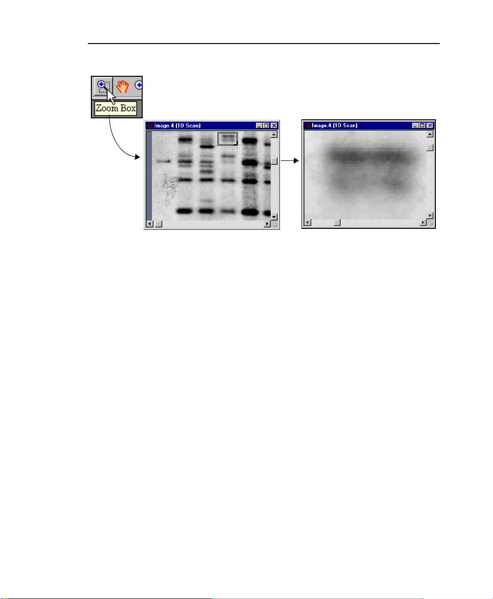
Zoom Box
Use Zoom Box to select a small area of the image to magnify so that it fills the entire
image window.
Click on the Zoom Box button on the main toolbar or select the command from the
View menu. Then drag the cursor on the image to enclose the area you want to
magnify, and release the mouse button. The area of the image you selected will be
magnified to fill the entire window.
3-2
Page 54
Chapter 3. Viewing and Editing Images
.
1. Click on Zoom Box button.
2. Drag box on image. 3. Boxed region is magnified to fill window
Fig. 3-2. Zoom Box tool.
Zoom In/Zoom Out
These tools work like standard magnifying tools in other applications.
Click on the Zoom In or Zoom Out button on the main toolbar (or select from the
View menu). The cursor will change to a magnifying glass. Click on an area of the
image to zoom in or out a defined amount, determined by the setting in the
Preferences dialog (see section
2.5, Preferences).
Grab
This tool allows you to change the position of the image in the image window. Select
Grab from the main toolbar or View menu. The cursor will change to a “hand”
symbol. Drag the cursor on the image to move the image in any direction.
Arrow Keys
You can also move the image inside the image window by using the Arrow keys on
the keyboard. Click on an arrow button to shift the image incrementally within the
window. The amount the image shifts is determined by the Pan % setting in the
Preferences dialog (see section
2.5, Preferences).
3-3
Page 55

Quantity One User Guide
View Entire Image
If you have magnified part of an image or moved part of an image out of view, select
View Entire Image fro m the main toolbar or View menu to return to the original, full
view of the image.
Centering an Image
You can center the image window on any point in an image quickly and easily using
the F3 key command. This is useful if you are comparing the same region on two gel
images and want to center both image windows on the same point.
Position the cursor on the poi nt on the image that you want at the center of the image
window , then press the F3 key. The image will shift so that point is at the center of the
image window.
Imitate Zoom
T o magnify the same area on multiple images at the same time, use the Imitate Zoom
command on the Window menu.
First, adjust the magnification in one of the images. Then, with that image window
still selected, select Imitate Zoom. The zoom factor and region of the selected image
will be applied to all the images.
Note: Imitate Zoom only works on images with similar dimensions.
Tiling Windows
If you have more than one image open, the Tile commands on the Window menu
allow you to arrange the images neatly on the screen.
Select Tile to resize all the windows and arrange them on the screen left to right and
top to bottom.
Select Tile Vertical to resize all windows and arrange them side-by-side on the
screen.
Select Tile Horizontal to resize all windows and stack them top-to-bottom on the
screen
3-4
Page 56

Chapter 3. Viewing and Editing Images
3.2 Density Tools
The density tools on the View > Plot Densi ty submenu and the Density Tools toolbar
are designed to provide a quick measure of the data in a gel image.
Fig. 3-3. Density tools on the menu and toolbar.
Note: The density traces will be slightly different than the traces for functions such as
Plot Lane or Plot Band, because the sampling width is only one image pixel.
Density at Cursor
Select Density at Cursor and click on a band or spot to display the intensity of that
point on the image. It also shows the average intensity for a 3 x 3 pixel box centered
on that point.
Density in Box
Select Density in Box and drag a box on the image to display the average and total
intensity within the boxed region.
Plot Density Distribution
Select Plot Density Distribution to display a histogram of the signal intensity
distribution for the part of the image displayed in the image window. The average
intensity is marked in yellow on the histogram.
The histogram will appear along the right side of the image. Magnify the image to
display the data for a smaller region.
3-5
Page 57

Quantity One User Guide
Plot Cross-section
Select Plot Cross-section and click or drag on the image to display an intensity trace
of a cross-section of the gel at that point. The horizontal trace is displayed along the
top of the image, and the vertical trace is displayed along the side of the image.
The intensity at the point you clicked on is displayed, as is the maximum intensity
along the lines of the cross-section.
Click on button, then
click or drag on the image.
Fig. 3-4. Plot Cross-section tool.
Plot Vertical Trace
Select Plot Vertical Trace and click or drag on the image to plot an intensity trace of
a vertical cross-section of the image centered on that point.
3.3 Showing and Hiding Overlays
To conceal all plots, traces, info boxes, and overlays on an image, select Hide
Overlays from the main toolbar or View menu.
3-6
Page 58

Chapter 3. Viewing and Editing Images
Note: Click once on Hide Overlays to conceal the overlays. Click twice to deassign
any function that has been assigned to the mouse.
To redisplay the lane and band overlays, select Show Lanes and Bands from the
View menu or main toolbar.
3.4 Multi-Channel Viewer
The Multi-Channel Viewer can display different types and levels of fluorescence in a
gel that has been imaged at different wavelengths. You can merge the data from up t o
three different images of the same gel.
Note: The gel images being compared must be exactly the same size. When changing
image filters, be careful not to move the gel. If the images are not exactly the
same size, you can use the Crop tool (see Section
resize them.
With at least one image open, select Multi-Channel Viewer from the View menu.
The first open image will be displayed in the viewer window using the Red channel,
and the image name will be displayed in the field at the top of the viewer.
3.9.a, Cropping Images) to
3-7
Page 59

Quantity One User Guide
Fig. 3-5. Multi-Channel View er.
Note: The color channel used to display the image in the viewer has no relation to the
filter used to capture the image. The red, green, and blue channels are only used
to distinguish different images.
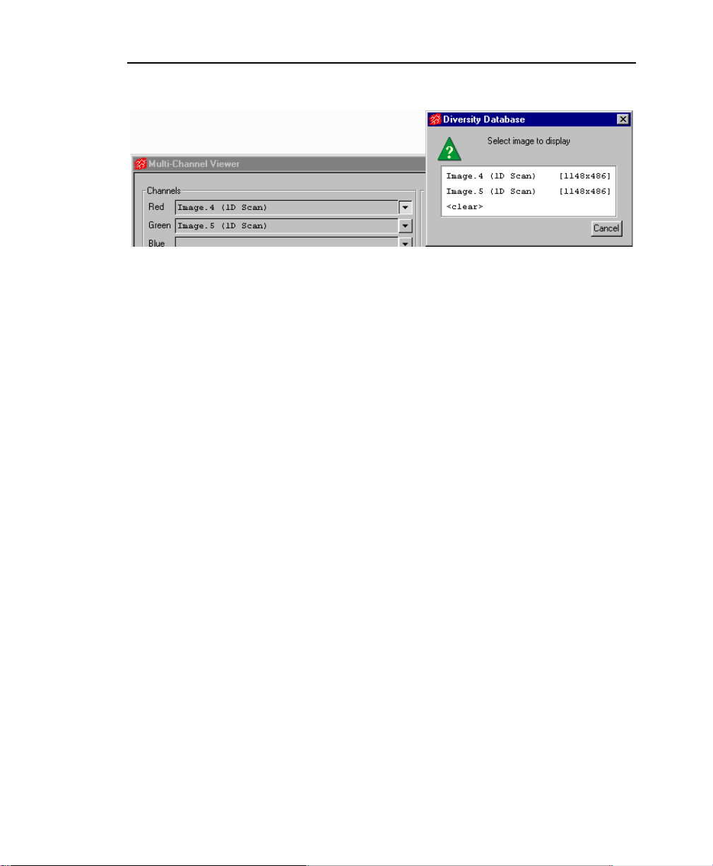
To add another image to the viewer, make sure the image is open and click on the
pulldown button next to the Green or Blue name field. Select the image name from
the pulldown list. Add a third image using the same procedure.
3-8
Page 60
Chapter 3. Viewing and Editing Images
Fig. 3-6. Selecting images to display in the viewer.
T o reassign the dif ferent images to dif ferent chann els, use the pulldown bu ttons to the
right of the name fields. Select <clear> from the pulldown list to remove an image
from that channel of the viewer.
Viewing Options
To remove a particular color channel from the display, click in the checkbox
associated with that channel to deselect it.
Select the Auto-Scale Image When Assigned checkbox to automatically adjust the
brightness and contrast of each loaded image based on the data range in the image.
This invokes the Auto-scale command from the Transform dialog (see section
Transform) when an image is first opened in the viewer . Note that this setting affects
only how the image is displayed in the viewer, not the actual data.
3.8,
Note: If you deselect this checkbox, any images currently displayed will remain auto-
scaled. Click on the Transform button in the viewer and click on the Reset
button in the Transform dialog to undo auto-scaling.
Buttons for various viewing tools are included in the Multi-Channel Viewer. Tools
such as Zoom Box and Grab will change the display of all the imag es in the viewer at
once.
Click on the Transform button to open the Transform dialog. In the dialog, you can
adjust the display of each channel indep enden tly by s electing the appropriate channel
option button. Similarly, the Plot Cross-section command will report the intensity of
each channel separately.
3-9
Page 61

Quantity One User Guide
Exporting an d Printing
Click on the Export button to export a 24-bit TIFF image of the merged view. This
will open a version of the Export to TIFF dialog (see section
Image). Note that you cannot export data from the Multi-Channel Viewer—only the
current view of the image (designated as Publishing Mode in the Export dialog). The
colors in the viewer will be preserved in the exported TIFF image.
To print a copy of the merged view to a color or grayscale printer, click on the Print
button.
11.5, Export to TIFF
3.5 3D Viewer
The 3D Viewer allows you to see a three-dimensional rendering of a portion of your
image. This is important for such instances as determining whether a selected band is
actually two or more separate bands.
To see a 3D rendering of a portion of your image, select 3D Viewer from the View
menu. Your curser turns into a crosshair. Click and drag your curser over the image
area you would like to view creating a box.
Note: viewing a large area of your image may reduce performance.
• To reposition the box, position your cursor at the center of the box. The cursor
appearance will change to a multidirectional arrow symbol. You can then drag
the box to a new position.
• To resize the box, position your cursor on a box corner. The cursor appearance
will change to a bi-directional arrow. You can then drag that corner in or out,
resizing the box.
• To redraw the box, position your cursor outside the box and click once. The box
disappears, and you can then draw a new box.
To view the selected area, position your cursor inside the box slightly off-center. The
cursor appearance will change to an arrow. Click once to open the 3D Viewer.
3-10
Page 62

Chapter 3. Viewing and Editing Images
Fig. 3-7. 3D Viewer
3.5.a Positioning the Image
Use your mouse or keyboard to reposition and rotate the image.
Windows
• Rotate the image - Left click and drag to rotate the image.
• Reposition the image - Right click and drag to reposition the image.
3-11
Page 63

Quantity One User Guide
• Zoom in/out - T o zoom in or out, Click the center mouse button or roll the wheel.
If you do not have a three button mouse or a mouse with a wheel, hold down the
shift key and left click and drag to zoom in or out.
Macintosh
• Rotate the image - Click and drag to rotate the image.
• Reposition the image - Ctrl>click and drag to reposition the image.
• Zoom in/out - Shift>click and drag to zoom in or out.
3.5.b Display Mode
The 3D Viewer window allows you to view the image in three different modes; wire
frame, lighting, and textured.
• Wire-frame shows the image in a transparent frame view.
• Light ing shows the image with different areas of light and shadow depen ding on
the angle of view. Use the slider bar to adjust the intensity of the lighting .
• Texture gives the image texture.
Use the Scale function to scale the image. This is useful for viewing shallow spots in
the 3D Viewer.
If you lose the image becaus e y ou mov e d it too far past the window bo rder, or rotated
it and disoriented the view, click Reset View to return th e image to the or iginal view.
Note: Reset view does not change the scale factor. To reset the scale factor, close the
3D Viewer and click the box again to re-open the 3D Viewer with the original
scale factor.
3.6 Image Stack Tool
Use the Image Stack Tool to scroll through a series of related gel images. You can
easily compare bands that appear , disappear , or chang e size in differen t gels run under
different conditions.
3-12
Page 64

Chapter 3. Viewing and Editing Images
Note: The images should be close to the same size, with bands in the same relative
positions. You can use the Crop tool to resize images.
With all the images open, select Image Stack Tool from the View menu. The Image
Stack Tool window will open.
Fig. 3-8. Image Stack Tool.
In the Image Stack Tool window, all open gels are listed in the field to the right of the
display window. To select an image to display, click on a gel name. The name will
appear highlighted with an arrow and the image will appear in the window.
Click on another gel name t o display that i mage.
Buttons for various viewing tools are aligned next to the Image Stack Tool window.
These commands will change the display of all the images in the stacker at once (e.g.,
magnifying one image will magnify the same relative area in all the images).
3-13
Page 65

Quantity One User Guide
Using the controls below the list of names, you can reorder the images and/or scroll
through them in the stacker.
Reordering Images
To reorder the images in the stacker, first select an image name in the list, and then
click on the Move displayed image arrow buttons to move it up or down in the list.
Image Playback
Using the controls under Playback, you can scroll through the images in the stacker.
First, highlight some or all of the gel names u sin g Shift-click or Ctrl-click key
commands. With multiple images selected, the Step arrow buttons become active.
Click on the arrow buttons to scroll through the list of selected gels.
Alternatively, click on the Auto checkbox next to the arrow buttons to begin
automatically scrolling through the list. Y ou can adjust the auto-scroll speed using the
Slow/Fast slider.
3.7 Colors
Select Colors from the Edit menu to open a dialog i n w hich you can adjust the colors
of the image, as well as windows, buttons, overlays, and other features of the display.
3-14
Page 66

Chapter 3. Viewing and Editing Images
Fig. 3-9. Colors dialog.
Selecting a Color Group
In the Colors dialog, click on the Color Group button to select the colors of a
particular group of objects (e.g., pop-up boxes, image colors, etc.).
Fig. 3-10. List of Color Groups.
Click on a color group in the list to select it.
3-15
Page 67

Quantity One User Guide
Changing a Colo r
After you have selected the color group to change, click on the specific color button.
In the Color Edit dialog, adjust the RGB values of the color you selected.
Fig. 3-11. Color Edit dialog.
Saving/Selecting a Defined Set of Colors
After you have changed t he colors withi n color groups , you can s ave these settin gs for
future use on other images . The Colormap Name field displa ys the name of a define d
set of colors and color groups. There are several predefined colormaps, or you can
create your own.
To select a predefined colormap, click on the Load button.
3-16
Page 68

Chapter 3. Viewing and Editing Images
A user-defined set of colors
Fig. 3-12. Selecting a Colormap.
From the list displayed, click on the set of colors you want to apply.
To create your own colormap, adjust the colors within the color groups as described
above and type in a new colormap name. Click on OK to apply the changes.
To remove a colormap, click on the Delete button. Select the colormap to be deleted
from the displayed list. A pop-up box will ask you to confirm the deletion.
To return to the Standard colormap, click on the Reset button. All colors will reset
to their default values.
3.8 T ransform
Use the Transform dialog to adjust the image brightness and contrast and opti mize the
image display. These controls affect the image display only, and will not change the
underlying data.
With an image open, select Transform from the Image menu or main toolbar.
3-17
Page 69

Quantity One User Guide
Fig. 3-13. Transform command.
The Transform dialog contains a Preview Window, a Frequency Distribution
histogram, a Transform Plot, and three main methods of optimizing the image: Auto-
scale, High and Low sliders, and a Gamma slider. You can use these controls to
adjust the way the software transforms raw image data into the visual display.
3-18
Page 70

Chapter 3. Viewing and Editing Images
Transform Plot
Frequency Distribution histogram
Preview Window
Auto-scale
Fig. 3-14. Transform dialog.
3.8.a Transform Subwindows
Preview Window
The Preview Window s hows a smaller v iew of the same image that is displayed in the
main image window. Changes in the controls are automatically reflected in the
Preview Window. They are only applied to the main image when you click on OK.
3-19
Page 71

Quantity One User Guide
You can use viewing tools such as Zoom Box, Grab and View Entire Image in the
Preview Window just as you can in the main image window, to focus on particular
regions of interest.
Frequency Distribution Histogram
The Frequency Distributi on his togram s hows the total data r ange in the i mage and t he
amount of data at each point in the range. In a typical scan, there is a signal spike at
the left (“gray”) end of the histogram due to background noise.
Transform Plot
The Transform Plot is a logarithmic representation of how the raw pixel data are
mapped to the pixels of the computer screen.
3.8.b Transform Controls
Auto-scale
Click on the Auto-scale button to optimize the image automatically. The lightest part
of the image will be set to the minimum intensity (e.g., white), and the darkest will be
set to the maximum intensity (e.g., black). This enhances minor variations in the
image, making fine details easier to see. You can then “fine-tune” the display using
the High, Low, and Gamma sliders described below.
High/Low Sliders
If Auto-scale doesn’t give you the appearance you want, use the High and Low
sliders to redraw the image manually. Drag the High slider handle to the left to make
weak signals appear darker. Drag the Low slider handle to the right to reduce
background noise.
As you drag the sliders, the slider markers on the Frequency Distribution histogram
will move. Everything to the left of the Low marker will be remapped to minimum
intensity, while everything to the right of the High marker will be remapped to
maximum intensity. Using the histogram, you can position the markers at either end
of the data range in the image, and use the low slider to cut off the “spike” of
background noise.
3-20
Page 72

Chapter 3. Viewing and Editing Images
You can also type specific High and Low values in the text boxes next to the sliders.
Click anyw here on the slider bars to move the sliders incrementally.
Log High/Low Sliders changes the feedback from the slider handles, so that when
you drag them, the slider markers move a shorter distance in the histogram. This
allows for finer adjustments when the data is in a narrow range.
In this example,
the range of
data in the image
is very limited
Low slider remaps background noise to white High slider remaps weaker signals to black
Can better distinguish background
noise from real data
Fig. 3-15. Two views of the Frequency Distribution histogram.
Low-High magnifies
area between sliders
3-21
Log scaling enables you to
better distinguish peaks
Page 73

Quantity One User Guide
Gamma Slider
Some images may be more effectively visualized if their data are mapped to the
computer screen in a nonlinear fashion. Ad just the Gamma slider handle to expand or
compress the contrast range at the dark or light end of the range. This is reflected in
the Transform Plot and Preview Window.
3.8.c Other Features
Full Scale and Low-High
The Full Scale and Low-High option buttons adjust how the range of data in the
image is displayed in the Freq uenc y Dist ribution hist ogram a nd Transform Plot. They
do not change how the data is displayed in the image window.
Select Full Scale to adjust the displays so that they show the full intensity range of the
image.
Select Low-High to magnify the range between the Low and High sliders. This
makes it easier to view the data if it does not occupy the full intensity range of the
image.
Log
The Log checkbox changes the way the data is displayed in the histogram so you can
better discern subtle changes in signal intensity.
Image Max/Min and Units
Image Max and Min display the range of intensity in the gel image.
The image units are determined by the type of scanner used to create the image. For
images measured in O.D.s, you can display the maximum and minimum O.D values
in the image by selecting the Calibrated Quantity checkbox. If this box is
unselected, the maximum and minimum numeric pixel values are displayed.
3-22
Page 74

Chapter 3. Viewing and Editing Images
Image Color
Click on this button to open a list of colormaps, which you can define using the
Colors command on the Edit menu (see section
the list to change the image in both the Transform window and the image window.
3.7, Colors). Select a colormap from
Invert Display
Select the Invert Display checkbox to change light bands on a dark background to
dark bands on a light background, and visa versa. The image data will not change—
only the display.
Highlight Saturated Pixels
Select the Highlight Saturated Pixels checkbox to highlight areas of saturation in the
image in red.
Always Auto-Scale
Select this checkbox to automatically Auto-Scale every new image that you open.
The software will examine the data range in every image and optimize it accordingly.
This setting disables the other image-optimization controls in the Transform dialog.
Reset
To return to an unmodified view of the image, click on Reset.
3.9 Resizing and Reorienting Images
The Image menu and tool bar contain commands for cha nging the size and o rientat ion
of images.
3-23
Page 75

Quantity One User Guide
Fig. 3-16. Resizing and reorienting tools.
Note: Many of these commands will permanently change the image. You will be
prompted to confirm any permanent changes.
3.9.a Cropping Images
Use the Crop tool to eliminate unwanted parts of an image, such as border space
around the gel. You can also use this command to reduce the file size of an image.
Select Crop from the Image menu or toolbar. The cursor will change to a Crop
symbol.
Define the region to be cropped by dragging the cursor across the image, creating a
box. Everything outside the box will be deleted.
The dimensions of the crop area (in millimeters and number of pixels) and the file
size of the image inside the crop area are listed at the bottom of the crop box.
1. To reposition the crop box, position the cursor at the center of the bo x. The cursor
will change to a multidirectional arrow. Then drag the box to a new position.
3-24
Page 76

Chapter 3. Viewing and Editing Images
2. To resize the box, position the cursor on a box border line or corner. The cursor
will change to a bidirectional arrow. You can then drag the border or corner in or
out, resizing the box.
3. To redraw the box, position the cursor outside the box. The cursor will change
back to the Crop tool, and you can redraw the box.
After you are satisfied with the size of crop box, position the cursor inside the box
slightly off-center. The cursor will change to a scissors symbol. Then click to perform
the crop.
A pop-up box will prompt you to: (1) crop the original image, (2) crop a copy of the
original image, or (3) cancel the operation.
Fig. 3-17. Crop box and pop-up Crop dialog.
If you click on the Copy and Crop button, you will be prompted to enter the name
and version number of the image copy before cropping.
3-25
Page 77

Quantity One User Guide
Advanced Crop Commands
To ensure that your scans are exactly the same size and shape, you can use the tools
on the Image > Advanced Crop submenu to save the crop box from one scan and
apply it to others. These tools also allow you to crop a gel of the same scan.
To define and save a crop box and apply it to another scan:
1. Select Define Crop Area from the submenu and drag a crop box on an image.
Position the box as described in Cropping Images.
2. Select Place Crosshair from the submenu and click a landmark inside the b ox that
is present in all the gels you want to crop. This could be a spot or some other
image detail. The crosshair will make it easier to position the box in the other
images so that it encloses the same area.
3. Select Save Crop Settings from the submenu, enter a name for the current crop
settings in the pop-up box, and click Apply.
4. Complete the crop action in the current image by positioning your cursor inside
the box slightly off-center and clicking to perform the crop, as described in
Cropping Images.
5. Open or select the next image you want to crop, select Load Crop Settings from
the submenu, and select the name of the settings you saved. The crop box and
crosshair will appear on the image.
6. Reposition the cro p box so that the crosshair is correctly aligned with the
appropriate image object, then complete the crop as described in step 4 above.
To delete any crop settings you have saved, select Delete Crop Settings from the
submenu and choose the settings to be deleted from the list.
3.9.b Flipping and Rotating Images
Use the image flipping and rotating commands to reorient lanes and bands for proper
analysis.
Note: These actions will erase any analysis you have performed on the image. You will
be prompted to confirm the changes.
3-26
Page 78

Chapter 3. Viewing and Editing Images
Flipping
To flip the image right-to-left, select Horizontal Flip from the Image menu or
toolbar. To flip the image top-to-bottom, select Vertica l Flip.
90° Rotations
Select Rotate 90 Left, Rotate 90 Right, or Rotate 180 from the Image > Rotate
menu or Image toolbar to perform the specified rotation.
Custom Rotation
Use the Custom Rotation command to rotate the image in increments other than 90°.
Select Custom Rotation from the Image > Rotate submenu or Image toolbar. A
green “plus” sign will appear next to the cursor. Click on the image and a circular
overlay with an orange arrow will appear. A pop-up box will indicate the angle of
rotation in degrees and radians.
3-27
Page 79
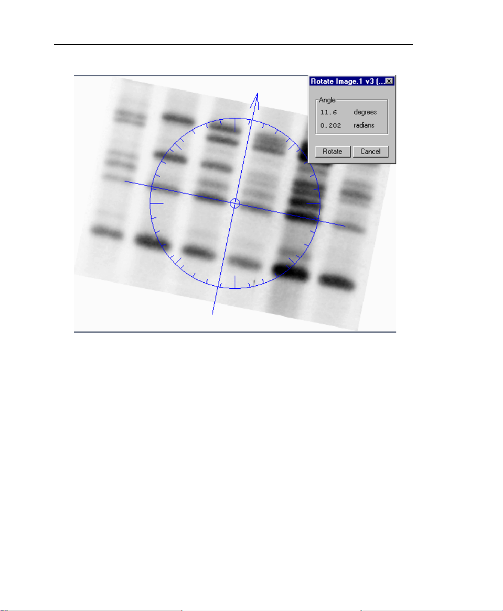
Quantity One User Guide
Fig. 3-18. Custom rotation; the arrow points in the direction of the new top of the image.
To perform the rotation, position the cursor on the arrowhead and drag. As you drag,
the arrow will rotate and the angle in the box will change. Position the arrow so that it
points in the direction of the new top of the image.
Note: To center the arrow on a particular point on the image (e.g., to align along a
particular lane), position the cursor on the point and press the F3 key. The center
of the arrow will shift to the new position.
To complete the rotation, click on the Rotate button in the pop-up box. Another
window will open containing the rotated image, and you will be prompted to save this
image under a new name or version number.
If you are not satisfied with the rotated image, close the window without saving and
start over.
3-28
Page 80

Chapter 3. Viewing and Editing Images
Note: Because an image is composed of square or rectangular pixels , Cust om Rot atio n
performs some minor smoothing on the image for rotations other than 90
any analysis performed on the image will be lost.
o
. Also,
3.10 Whole-Image Backgroun d Subtraction
Image background due to gel opacity, random signal noise, or other factors can
interfere with quantitation and data analysis. Quantity One has several tools for
subtracting background intensity from gel images. This section describes whole
image background subtraction. You can also subtract background from individual
lanes (see section
7.4, Volume Background Subtraction).
Whole-image background subtraction is useful for reducing background resu lting
from the opacity of the carrier medium (film, gel matrix, or blot matrix) or film
fogging.
Note: Whole-image background subtraction permanently changes the image. You will
be prompted to confirm the change.
Select Subtract Background from the Image menu.
4.2, Lane-Based Background Subtraction) and bands (see section
3-29
Page 81

Quantity One User Guide
Fig. 3-19. Subtract Background dialog.
The Subtract Background dialog has a preview window, which contains a smaller
view of the image. Changes in the subtract background controls are reflected in the
preview window and are only applied to the main image when you click on OK.
3-30
Page 82

Chapter 3. Viewing and Editing Images
Auto-scale
Click on the Auto-scale button to automatically adjust th e Dark Contrast and
Background settings to optimal levels. You can then manually adjust these settings
using the other controls .
Dark Contrast Slider
Use the Dark Contrast slider to reveal the level of background in the image before
subtraction. This slider is similar to the High slider in the Transform dialog. Dr ag the
slider handle to the left to make faint signals appear stronger. Click on the slider bar to
move the slider incrementally, or type a value into the field next to the slider.
Note: The Dark Contrast slider itself does not eliminate background intensity;
therefore, the OK button will not activate if you only adjust this slider. If you
want to adjust the display contrast without subtracting background, use the
Transform command (see section
3.8, Transform).
Before adjustment: the image
seems clear of background
Fig. 3-20. Dark Contrast adjustment reveals true levels of background in the image.
After adjustment: background levels are
more apparent
3-31
Page 83

Quantity One User Guide
Background Slider
T o manu ally ad just th e back gro und subtr action levels , d rag the Background slider to
the right. You can also move the slider incrementally by clicking on the slider bar, or
type a specific value into the field next to the bar.
Objects with signal intensities lower than the subtraction level will be eliminated
from the image when you click on OK.
Background Box
Use the Background Box function to define a background area in the gel that is
representative of the background in the entire image. This method of subtraction is
useful for images with uniform backgrounds.
Click on the Background Box button, then drag on a background area of the image.
The average intensity of the pixels in the box will be used as the background level to
be subtracted from the entire image.
Background Stripe
The Background Stripe function is useful for gels in which the background changes
from top to bottom (e.g., gradient gels).
Click on the Background Stripe button, then drag on a backgroun d region to cr eate a
rectangular box down the length of the image. The average intensity of each
horizontal row of pixels in the stripe will be subtracted from each pixel in that row
across the entire gel. This way, if the image has more background at the bottom than
at the top, more background will be removed from the lower regions of the image.
Note: Make sure that the background stripe runs the entire length of the lanes down the
gel. The average of the topmost row in the stripe will be subtracted from all rows
above the stripe, and the average of the bottommost row will be subtracted from
all rows below.
The minimum and maximum intensities in the stripe are displayed next to the Min
and Max labels in the box. Also, the average intensity value for the entire stripe is
displayed next to Avg.
3-32
Page 84

Chapter 3. Viewing and Editing Images
Completing the Subtraction
When you are satisfied with the backgrou nd subtraction shown in the preview image,
click on OK. Because whole-image background subtraction is irreversible, you will
be prompted to subtract from the original image, subtract from a copy, or cancel the
operation.
If you choose Copy and Subtract, enter the name and/or version n umber for the new
copy in the pop-up box and click on OK to complete the command.
3.11 Filtering Images
Filtering is a process that removes small noise features on an image while leaving
larger features (e.g., bands) relatively unaffected. A wide range of filters are available
for removing different types of noise from images. Depending on the nature of your
data, you will probably need to use only one or two of the available filters. However,
you should experiment with several different filters before selecting the ones that
work best for your images.
The filtering commands are located on the Image menu and toolbar.
3-33
Page 85
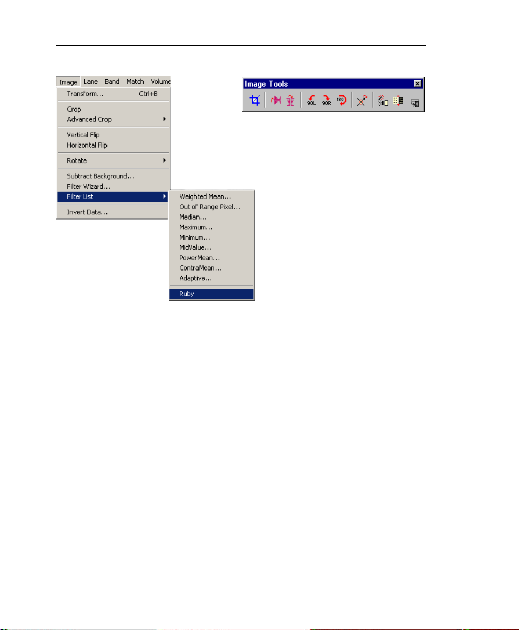
Quantity One User Guide
Fig. 3-21. Filtering commands.
Note: Since filtering is an irreversible process, you will be asked if you want to creat e a
copy of the original image before you filter. If you are experimenting with
various filters, you should create copies of the image and compare them side-byside. If you filter the original image and save it, you cannot r eturn to the or iginal,
unfiltered state.
3.11.a Filter Wizard
The Filter Wizard is designed to guide you through the filter selection process. First,
you identify the type of noise in the image. Next, select the size of the filter to use on
that noise. Finally, filter the image.
Select Filter Wizard from the Image menu or toolbar to open the dialog.
3-34
Page 86

Chapter 3. Viewing and Editing Images
Fig. 3-22. Filter Wizard dialog.
The dialog contains settings for identifying th e differe nt types of noise in the image. It
also includes a density distribution histogram of the noise in the image to aid in filter
selection.
Step I: Identify Noise Characteristics
The first step is to identify the type of noise in the image. Examine both the image and
the density distribution histogram, then select one, both, or neither of the following
checkboxes:
• Salt. This type of noise appears as specks that are lighter than the surrounding
background. The density distribution histogram of this type of noise displays
noise peaks at the high end of the range (right end of the plot). This type of noise
is common in electronic cameras with malfunctioning pixels. It can also be
3-35
Page 87

Quantity One User Guide
caused by dust or lint in the imaging optics or scratches on photographic film.
Salt is a type of outlier noise (see below).
• Pepper. This type of noise appears as specks that are darker than the surroundin g
background. The dist rib ution hist ogram o f th is ty pe of noise d ispla ys noi se p eaks
at the low end of the range (left end of the plot). Its causes are similar to thos e of
salt noise. Pepper is a type of outlier noise (see below).
Next, select one of the following option buttons to describe additional features of the
noise.
• Gaussian. The distribution histogram of this type of noise has a Gaussian profile,
usually at the bottom of the data range. This type of noise is usually an electronic
artifact created by cameras and sensors, or by a combination of independent
unknown noise sources.
• Uniform noise. This type of noise appears in the histogram as a uniform layer of
noise across the data range of the image.
• Outlier noise. This category of noise includ es salt an d pepp er no ise (see abov e).
The distribution histogram of this type of noise displays noise peaks at the high
and low ends of the range.
After you have identified the type of noise, go to the next step.
St ep 2: Sel e ct Filter Size
Image noise is filtered by means of a filtering window (or kernel), which is measured
in pixels. This filtering window slides across the image, processing th e pixels within
it.
The available filter dimensions range from 3 x 3 to 9 x 9 pixels. To select an
appropriate size, magnify a background region of the image so that you can see the
individual pixels. The filter size you select should be larger than the average noise
feature but smaller than the data features.
Note: A smaller filter will alter the image less than a larger filter. Large filters can result
in better suppression of noise, but can also blur desirable features in the image.
3-36
Page 88

Chapter 3. Viewing and Editing Images
Step 3: Begin Filtering
After you have completed the selections, the filter name and size will be displayed at
the bottom of the Filter Wizard dialog.
T o being filtering, click on the OK button. Because filter ing is an irreversible p rocess,
you will be prompted to filter the original image, filter a copy of the image, or cancel
the operation.
If you choose Copy and Filter, enter a name an d/or version number fo r the new copy
in the pop-up box and click on OK.
3.11.b Selecting a Filter Directly
If you know the type and size of filter you want, you can select it directly from the
Image > Filter List submenu. The submenu includes all the availa ble filters.
The types of filters are:
• Weighted Mean. This filter is useful for reducing Gaussian noise. It calculates
the weighted mean of the pixels within the filtering window and uses it to replace
the value of the pixel being processed.
• Out of Range Pixel. This filter is useful for suppressing salt-and-pepper noise;
its effect on Gaussian noise is minimal. This filter calculates the mean of the
pixel values in the filtering window, including the pixel being processed. If the
difference between the mean and the individual pixel value is above a certain
threshold, then the individual value is replaced by the mean.
• Median. Also useful for suppressing salt-and-pepper noise, this filter calculates
the median value of the pixels within the filtering window and uses it to replace
the value of the pixel being processed. The median filter produces very little
blurring if a small-sized window is selected.
• Maximum. This filter is useful for eliminating pepper noise in an image (it
worsens the effect of salt noise). It replaces the value of the pi xel being processed
with the maximum value of the pixels within the filtering window.
• Minimum. This filter replaces the value of the pixel being processed with the
minimum pixel value within the filtering window. This filter is useful for
eliminating salt noise in an image (it worsens the effect of pepper).
• MidValue. This filter is useful for suppressing uniform noise within an image;
however, it worsens the effect of pepper and salt. This filter replaces the value of
3-37
Page 89

Quantity One User Guide
the pixel being processed with the mean of the maximum and minimum pixel
values within the filtering window.
• PowerMean. This filter is useful for suppressing salt and Gaussian noise within
an image (it worsens the effect o f pepper nois e). I t replaces the value of the pixel
being processed with the power mean of the pixel values within the filtering
window.
• ContraMean. This filter is useful for suppressin g pepper and Gaussi an nois e
within an image (it worsens the effect of salt). It replaces the value of the pixel
being processed with the contra-harmonic mean of the pixel values within the
filtering window.
• Adaptive. This filter is useful for suppressing Gaussian noise and salt and/or
pepper within an image. If the image contains a mix of salt and pepper, select this
filter.
To begin filtering, select a filter type from the pull-down list. A pop-up box will
prompt you to select a filter size.
Fig. 3-23. Selecting a filter size.
Click on a button to select a size. (See, Step 2: Select Filter Size for guidance.)
Because filtering is an irreversible process, you will be prompted to filter the original
image, filter a copy of the image, or cancel the operation.
If you choose Copy and Filter, enter a name an d/or version number fo r the new copy
in the pop-up box and click on OK.
3-38
Page 90

Chapter 3. Viewing and Editing Images
3.12 Invert Data
The Invert checkbox in the Transform dialog (see “Invert Display” on page 23)
inverts the display of the image. However, in some cases you may need to invert the
actual image data.
If the image has light bands or spots on a dark background (i.e., the signal intensity of
the background is greater than the signal intensity of the sample), you need to invert
the data before analysis.
Select Invert Data from the Image menu or toolbar. This func tio n is reversib le. You
may need to use the Transform controls to adju st the appearance of the inverted
image.
3.13 Text Overlays
To create and display textual notes directly on the image, select Text Overlay Tools
from the Edit menu or main toolbar. This will open the Text Overlay Tools toolbar.
Select tool
Text tool
Line tool Alignment tools
Fig. 3-24. Text Overlay Tools toolbar.
Copy Paste
Creating a Text Overlay
To create a text overlay, click on the Text Tool, then click on the image at the spot
where you want the text to appear. This opens the Text Overlay Properties dialog.
3-39
Page 91

Quantity One User Guide
Text color
Background color
Fig. 3-25. Text Overlay Properties dialog.
To enter text, type in the main field. Use the buttons in the dialog to select the
properties of the text, including format, alignment, and justification.
Select the font style, font size, color of the text, and color of the background in the
text box using the pull-down lists.
After you have typed the text, click on OK. The text will appear on the image at the
spot where you originally clicked.
Editing a Text Overlay
To edit a text overlay, make sure the Text Tool or Select Tool is selected, and then
double-click on the overlay to open the Text Overlay Properties dialog. The existing
text will be displayed and can be edited.
Line Tool
You can use the Line T ool to draw a line between text and an image feature, or
between any two points of interest on the image.
Click on the Line Tool button, then drag on the image to create the line.
T o resize or ad just a line, make sure the Line Tool or Select Tool is selected, and then
position the cursor on one end of the line (marked by a circle) and drag.
3-40
Page 92

Chapter 3. Viewing and Editing Images
To add arrowheads to a line, make sure the Line Tool or Select Tool is selected, and
then double-click on the middle of the line. A dialog will pop up with options to add
arrowheads to one or both ends of the line.
Moving and Copying Text an d Lines
You can move, copy, or delete a single text overlay or line or a group of over l ays and
lines within an image. You can also copy and paste between images.
First, you must select the ob ject(s). C lick on th e Select Tool button. To select a single
overlay or line, click on it. To select multiple objects, either drag a box around them
or hold down the Shift key and clic k o n them i ndivi d uall y. When dragging to select a
group of objects, make sure that you completely surround all the objects to be
selected.
Each selected overlay/line will have a green border.
•To move the selected object(s), position the cursor over the selection and drag.
•To copy within an image, hold down the Ctrl key while dragging the selected
object(s). The copy will be created and dragged to the new position.
•To delete the selected object(s), press the Delete key.
•To copy between images, click on the Copy to Clipboard button, then open or
select the image you want to copy to and click on the Paste from Clipboard
button. The copied object(s) will be pasted into the new image in the same
relative position they were copied from.
Note: If you are pasting into an image with a different pixel size (i.e., resolution), you
will receive a message that the placement of the copy may not be exact. Click on
OK to complete the paste, then position the pasted objects manually.
Viewing Previously Created Text Overlays/Lines
Previously created text overlays and lines will appear on the image when you open
the Text Overlay Tools toolbar.
If you have concealed all overlays using the Hide Overlays command (section 3.3,
Showing and Hiding Overlays), click on any of the buttons on the Text Overlay Tools
toolbar to redisplay the text.
3-41
Page 93

Quantity One User Guide
3.14 Erasing All Analysis from an Image
To delete all analysis and overlays from an image (including any lanes, bands,
volumes, standards, text overlays, etc.), select Clear Analysis from the Edit menu.
Since this process is irreversible, you will be prompted to confirm the selection.
3.15 Sort and Recalculate
To update, renumber, and recalculate all lane and band information, select Sort and
Recalculate from the Edit menu.
3.16 Automation Manager
The Automation Manager allows you to save objects such as lanes, automated band
detection, standard bandsets, volume overlays, and text and line overlays in a
template file. These files can then be automatically applied to images either
individually or in batches. To open the Automation Manager, select
Analysis>Automation Manager.
3-42
Page 94

Chapter 3. Viewing and Editing Images
Fig. 3-26. Automation Manager dialog
3.16.a Step 1 - Select Template
The Select template field lists all the templates that are currently open. The
Automation Manager remembers the files that were open the last time the application
was open. To create a new template, click New. A new template appears in the list.
See Section
template. To open an existing template not currently in the list, click Open. This opens
the standard Open dialog. To remove a template from the list, click Close.
3.16.b, Step 2 - Edit Selected Template for how to modify a new
3.16.b S tep 2 - Edit Selected Template
Step 2, Edit Selected Template, lists the name of the currently selected template and
the list of options available to the template. To edit the template, check the option(s)
you would like to include and/or uncheck the option(s) you would like to remove
from the template.
3-43
Page 95
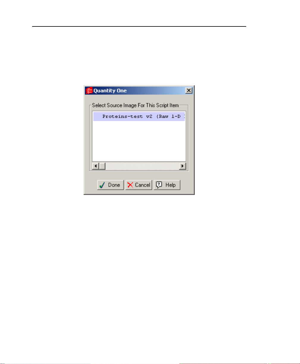
Quantity One User Guide
Use Single Image for Template
The Automation Manager allows you to specify a single image as the source for all
options you select. Checking the Use Single image for template box opens the Select
Source Image for this Script item dialog opens.
Fig. 3-27. Select an image
Make sure the image you select contains the object(s) you wish to apply to the
destination images.
If you wish to use options from multiple images, then uncheck the box labeled, Use
single image for template. As you check each option in step two you will be
prompted to select a source image for that option.
Note: The source image must be open when the option check box is selected. Once you
have finished checking options from a source, the source image can be closed.
When you are satisfied with your changes, click Save, or Save As to save it as a new
template. If this is a new template, you must enter a new name for the template when
you click Save. To change the name of a template, click Save As and enter a new
name.
3-44
Page 96

Chapter 3. Viewing and Editing Images
Default Automation
The default automation template is applied to the currently active image when you
select Analysis>Apply Default Automation. To set a new default template, highlight
the desired template in the Automation Manager and click Set as Default.
To run the default automation template on the currently active image, select Apply
Default Aut omation from the Analysi s menu.
Once a default template is chosen, The Automation Manager does not need to be open
to be applied, nor do you need to select a default each time Quantity One opens as it
remembers the default from the last open session of the application.
3.16.c Step 3 - Select Images
This portion of the Automation Manager lists the currently open images. Select the
images to which you wish to apply the selected template. Use ctrl>click and
shft>click to select more than one image, or click Select All to select all the images in
the list.
3.16.d Step 4 - Apply Selected Template
Click Apply to apply the selected template in step 1 to the selected images in step 3.
3-45
Page 97

Quantity One User Guide
3-46
Page 98

4. Lanes
Before you can use many of the analysis functions, you must first define lanes and
bands on the gel image. This chapter describes the tools for defining lanes.
Note: If you want to compare bands across lanes (using standards or band matching),
the lane lines should be approximately the same length, with their starting points
aligned across the top of the image. This is important for calculating the relative
mobility of the bands. If gel wells are visible in the image, you should center the
start points of the lane lines on the wells and position the ends of the lanes
slightly below the last band for best results.
4.1 Defining Lanes
You can define lanes individually or as part of a frame. The functions for doing this
are on the Lane menu and toolbar.
Fig. 4-1. Lane menu and toolbar.
In Quantity One, lanes are defined by red lane lines overlaid on a gel. The lane lines
can be created individually (see section
as part of a lane frame.
4.1.c, Single Lanes), or they can be created
4-1
Page 99
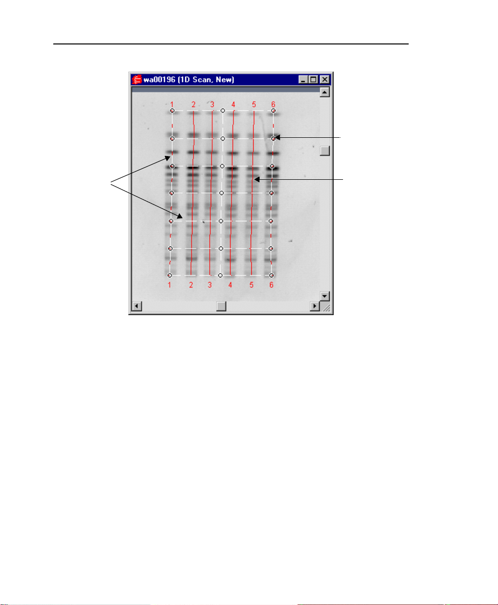
Quantity One User Guide
Anchor point
Border and
anchor lines
(in white)
Fig. 4-2. Features of a lane frame.
Lane (in red)
4.1.a Lane Frames
The fastest way to define all the lanes on a gel is to create a lane frame using the Auto
Frame Lanes command. If this command do esn’t work well on your images, you can
create and place a lane frame manually.
Auto Frame Lanes
Note: Auto Frame Lanes works best on gels with large numbers of clearly defined
lanes and bands. Also, the lanes should be reasonably vertical and contain
approximately the same amount of sample.
Select Auto Frame Lanes from the Lane menu or toolbar. The program will
automatically detect the lanes and place a frame over them.
4-2
Page 100

Chapter 4. Lanes
The lane frame contains individual lane lines numbered sequentially from left to
right. The border and anchor lines of the frame are marked with dashed white lines,
the lanes are solid red lines, and each anchor point (interior and corner) is marked
with a circle.
The top and bottom of the frame are parallel with the top and bottom of the image.
However, the interior anchor points and lines will “bend” the frame to follow the
actual lanes in the gel, compensating for any curving or distortion in the gel.
If Auto Frame Lanes detects too few or too many lanes, you can add or delete lanes
using the single lane commands (see section
If Auto Frame Lanes does not work on the image, you will be prompted to create a
lane frame manually. To delete the lane frame, select Clear Analysis from the Edit
menu.
4.1.c, Single Lanes).
Manual Frame Lanes
If Auto Frame Lanes does not work with your images, you can frame the lanes
manually.
Select Frame Lanes from the Lane menu or toolbar. In the dialog, enter the number
of lanes in the gel and click on OK.
Fig. 4-3. Frame Lanes dialog.
4-3
 Loading...