

Page 1
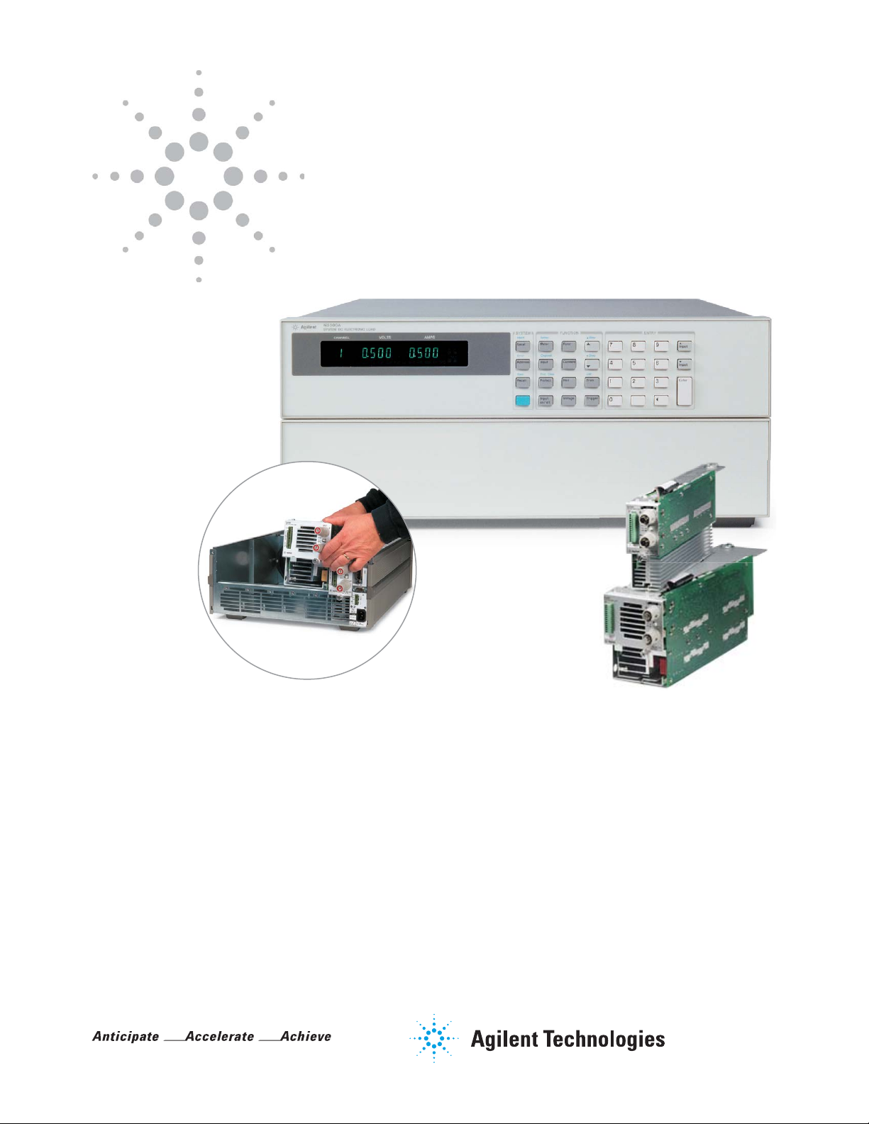
Agilent N3300 Series
DC Electronic Loads
Data Sheet
Increase your manufacturing test throughput with
fast electronic loads
• Increase test system throughput
• Lower cost of ownership
• Decrease system development time
• Increase system reliability
• Increase system flexibility
• Stable operation down to zero volts
• DC connection terminal for ATE applications
Page 2
Increase Test Throughput
Today’s high volume manufacturing
requires optimization of test system
throughput, to maximize production
volume without increasing floorspace.
The N3300 Series electronic loads
can help you in a number of ways to
achieve this goal.
Reduced command processing time:
Commands are processed more
than 10 times faster than previous
electronic loads.
Automatically execute stored
command sequences: “Lists” of
downloaded command sequences can
execute independent of the computer,
greatly reducing the electronic load
command processing time and computer interaction time during product
testing.
Programmable delay allows for
either simultaneous or sequential
load changes: This is the most
multiple output DC power supplies,
simulating real-life loading patterns,
with a minimum of programming
commands.
Buffer measurement data: Voltage,
current, and power measurements
can be buffered for later readback
to the computer, reducing computer
interaction.
Control measurement speed vs.
accuracy: Decrease the number of
measurement samples to achieve
greater measurement speed, or
increase the number of samples to
achieve higher measurement accuracy. You can optimize your measurements for each test.
Control rising and falling slew rates
separately: Reduce rate of loading
change when necessary for DUT
stability or to simulate real life conditions, but otherwise change load
values at maximum rate.
Increase System
Flexibility…for Both
Present and Future
Requirements
Most power supply and battery
charger test systems designed today
need to test a variety of products
and/or assemblies. In the future,
additional products or assemblies
may be needed. A flexible family
of electronic loads makes present
system design and future growth
much easier.
Test low voltage power supplies:
The N3300 Series electronic loads
operate with full stability down to
zero volts. Many other electronic
loads available today have been found
to become unstable in the operating
region below one volt. When designing power supply test platforms, the
trend towards lower voltage requirements should be taken into account.
Refer to the specification and
supplemental characteristic tables
for details of lower voltage operating
characteristics.
Choose DC load connection method:
Automatic test systems need
consistency and reliability. Option
UJ1 8 mm screw connectors provide
a simple screw onto which your
wires, terminated with insulated ring
terminals, may be securely mounted.
This optional connector is specifically
designed for test systems. Wires may
exit the plastic cover in any direction,
and multiple wires may be placed on
each screw terminal for easy parallel
load connections. Up to AWG 4 wire
may be used.
Applications which require repeated
connections/disconnections are better suited to the standard connector.
The standard connector accepts an
unterminated wire, and may be handtightened. This connector is specifically designed for bench applications
and short-term automated tests.
Standard DC connectors
Option UJ1 8 mm screw connectors
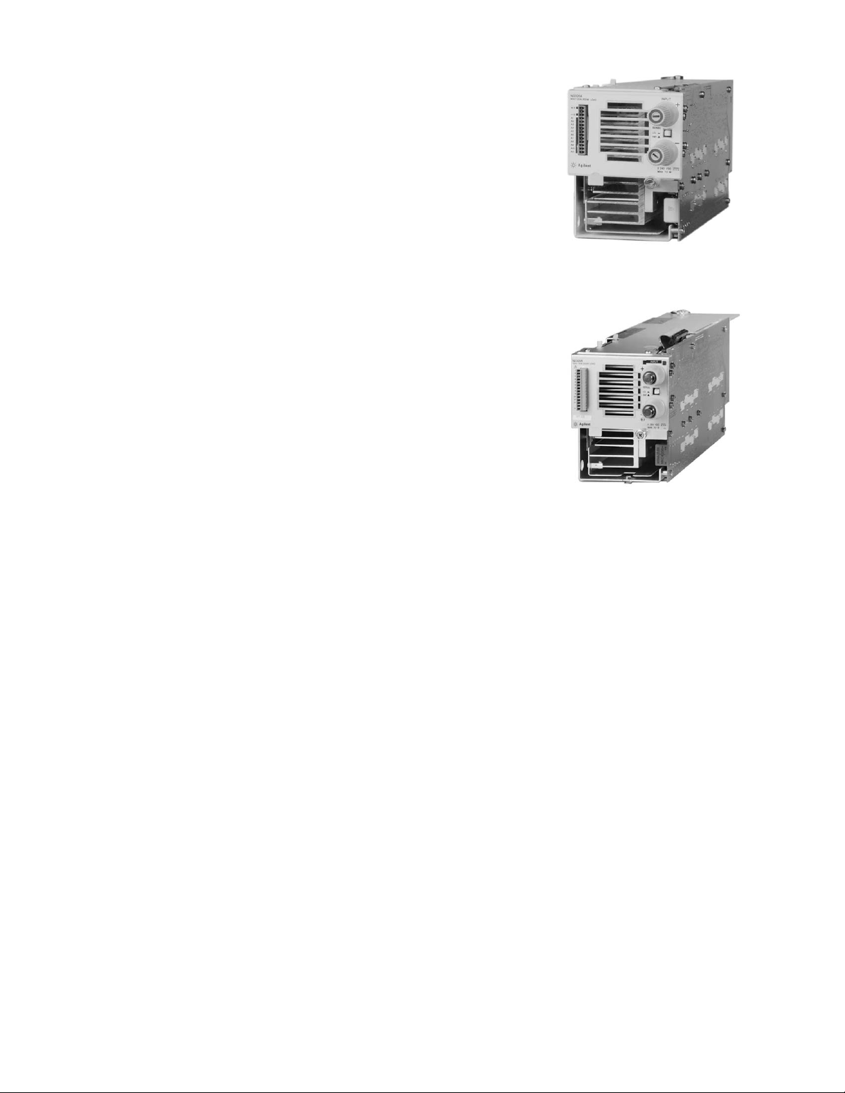
Design a system to test a variety
of products: This series consists of
2 mainframes and 6 modules. The
N3300A mainframe is full rack width.
It has 6 slots. The N3301A mainframe
is half rack width. It has 2 slots.
Any assortment of the 6 different
modules can be configured into these
mainframes, up to the slot capacity.
The N3302A (150 watts), N3303A
(250 watts), N3307A (250 Watts) and
N3304A (300 watts) each require
one slot. The N3305A (500 watts)
and the N3306A (600 watts) each
require 2 slots. The electronic load
can be configured to supply exactly
what you need now, and this modular
design also allows for easy future
reconfiguration.
Test high current power supplies:
Electronic load modules can be operated in parallel to provide additional
current sinking capability.
2
Page 3

Control the electronic load how you
want to: GPIB, RS232, and manual
use of the front panel all provide
complete control of these electronic
loads. There are also analog programming and monitoring ports for those
applications that utilize nonstandard
interfaces, require custom waveforms, or utilize process control
signals. Custom waveforms can also
be created by downloading a “List” of
load parameters. In addition, there is
a built-in transient generator, which
operates in all modes.
Quickly create powerful and
consistent software: All Agilent
Technologies electronic loads use
the SCPI (Standard Commands for
Programmable Instruments) command set. This makes learning the
commands easy, because they are
the same format as all other SCPI
instruments. The resulting code is virtually self-documenting, and therefore
easier to troubleshoot and modify
in the future. Plug-n-Play drivers are
also available to help you to integrate
the loads into your standard software
packages.
Make Measurements
Easily and Accurately
The 16-bit voltage, current and power
measurement system provides both
accuracy and convenience. The
alternative is using a DMM (digital
multimeter) and MUX (multiplexer)
along with a precision current shunt
and a lot of extra wiring. Avoiding
this complexity increases system
reliability and makes the system
easier to design and support. Current
measurements in particular are
more consistently accurate using
the electronic load’s internal system,
because the wiring associated with
an external precision current shunt
may pick up noise.
Measure with all load modules
simultaneously: Testing multiple
output DC power supplies and DC
to DC converters can be very time
consuming if each output must be
tested sequentially. If measurements
are being made through a MUX using
one DMM, this is what will happen.
Using the built-in measurement
capabilities of the N3300 electronic
loads, all outputs can be measured
simultaneously. Alternatively, multiple
single output power sources can be
tested simultaneously.
Observe transient behavior using
waveform digitization: Transient
response and other dynamic tests
often require an oscilloscope. The
N3300 has a flexible waveform
digitizer with a 4096 data point
buffer for voltage and a 4096 data
point buffer for current. Under many
circumstances, this internal digitizer
will be adequate for power supply
test needs. Current and voltage are
digitized simultaneously, and the
sampling rate and sample window
are programmable. Some analysis
functions are provided, including
RMS, max and min.
Measure voltage and current
simultaneously: The N3300 measure-
ment system has individual but linked
current and voltage measurement
systems. This means that voltage
and current measurements are taken
exactly simultaneously, which gives
a true picture of the power supply
under test’s output at a particular
moment in time. Some other electronic loads which feature internal
measurement systems actually take
current and voltage measurements
sequentially, and therefore do not give
as accurate a picture of momentary
power.
3
Page 4
Specifications
Table A-1 lists the specifications for the different load models. Specifications
indicate warranted performance in the 25 °C ± 5 °C region of the operating
temperature range. Specifications apply to normal and transient modes unless
otherwise noted.
Table A-1
N3302A N3303A N3304A N3304-J01
Special
order option
N3305A N3306A N3307A
Input ratings
Current 0–30 A 0–10 A 0–60 A 0–60 A 0–60 A 0–120 A 0–30 A
Voltage 0–60 V 0–240 V 0–60 V 0–80 V 0–150 V 0–60 V 0–150 V
Maximum power @ 40 °C
1
150 W 250 W 300 W 300 W 500 W 600 W 250 W
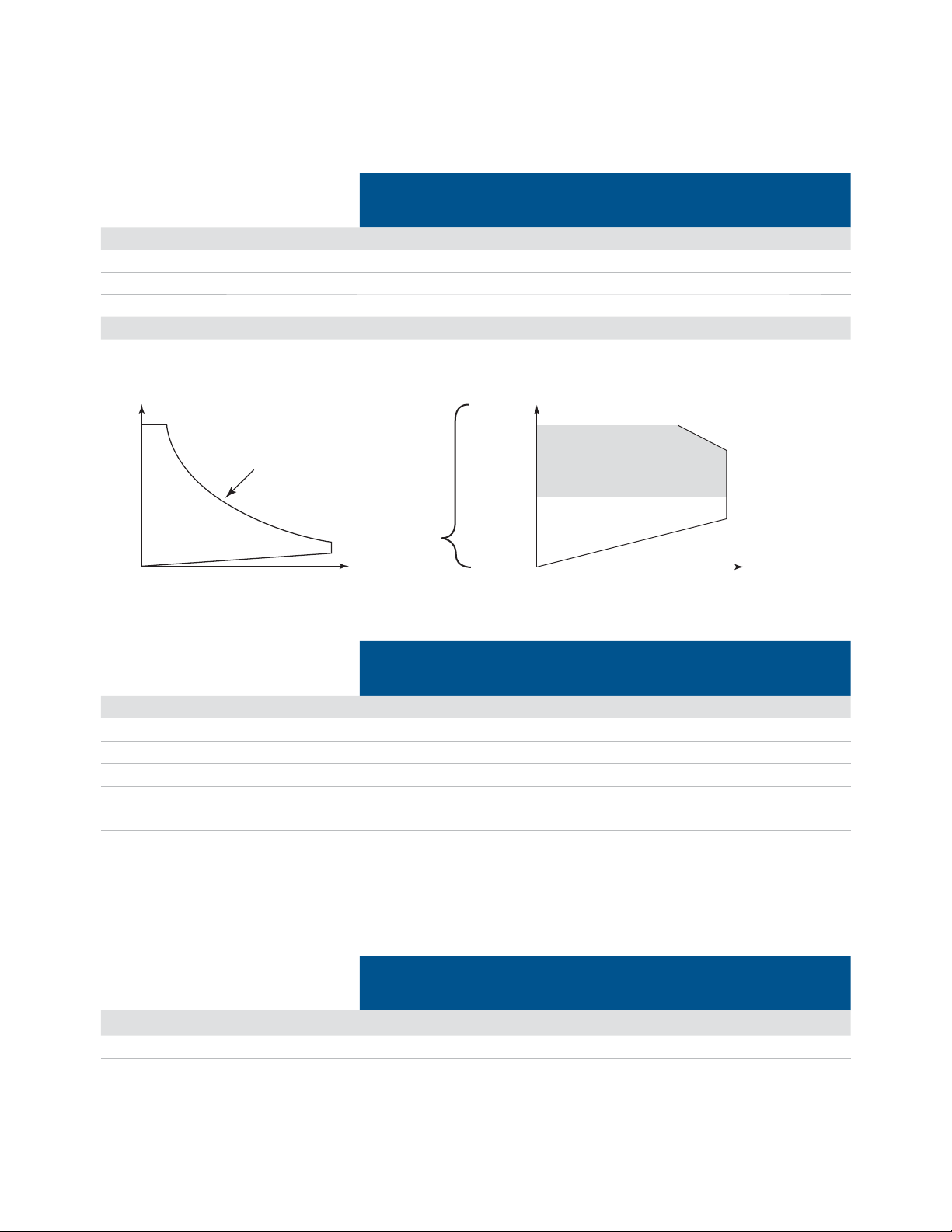
Input characteristic
Operating contour Derated current detail
Voltage
Full
scale
Max. power contour
0
Current
Full
scale
Voltage
Full
scale
All specifications apply
3
Slew rate limitations apply
2
(see Table A-2)
1
0
Current
Full
scale
N3302A N3303A N3304A N3304-J01
Special
order option
N3305A N3306A N3307A
Specified current @ low voltage operation
2.0 V
1.5 V
1.0 V
0.5 V 7.5 A 2.5 A 15 A 15 A 15 A 30 A 7.5 A
0 V 0 A 0 A 0 A 0 A 0 A 0 A 0 A
1. Maximum continuous power available is derated linearly from 100% of maximum at 40 °C, to 75% of maximum at 55 °C.
30 A 10 A 60 A 60 A 60 A 120 A 30 A
22.5 A 7.5 A 45 A 45 A 45 A 90 A 22.5 A
15 A 5 A 30 A 30 A 30 A 60 A 15 A
Table A-1 states that maximum current is available down to 2 volts. Typically,
however under normal operating conditions, the load can sink the maximum
current down to the following voltages:
N3302A N3303A N3304A N3304-J01
Special
order option
N3305A N3306A N3307A
Typical minimum operating voltage @ full scale current
1.2 V 1.2 V 1.2 V 1.2 V 1.4 V 1.4 V 1.4 V
4
Page 5

Table A-1
Specifications (continued)
Constant current mode
Low range/High range
Regulation
Low range accuracy 0.1% +
High range accuracy
0.1% +
Constant voltage mode
Low range/High range
Regulation
Low range accuracy 0.1% +
High range accuracy
0.1% +
Constant resistance mode
Range 1
(I > 10% of current rating)
Range 2
(I > 1% of current rating)
Range 3
(I > 0.1% of current rating)
Range 4
(I > 0.01% of current rating)
2
2
1
1
0.05% +
0.05% +
1
0.05% +
0.1% +
Current measurement
Low range/High range
Low range accuracy
High range accuracy
Voltage measurement
Low range/High range
Low range accuracy 0.05% +
High range accuracy
Power measurement
Accuracy
N3302A N3303A N3304A N3304-J01
N3305A N3306A N3307A
Special order
option
1
3 A/30 A 1 A/10 A 6 A/60 A 6 A/60 A 6 A/60 A 12 A/120 A 3 A/30 A
10 mA 8 mA 10 mA 10 mA 10 mA 10 mA 10 mA
5 mA 4 mA 7.5 mA 7.5 mA 7.5 mA 15 mA 7.5 mA
10 mA 7.5 mA 15 mA 15 mA 15 mA 37.5 mA 15 mA
1
6 V/60 V 24 V/240 V 6 V/60 V 8 V/80 V 15 V/150 V 6 V/60 V 15 V/150 V
5 mV 10 mV 10 mV 10 mV 10 mV 20 mV 10 mV
3 mV 10 mV 3 mV 5 mV 10 mV 3 mV 10 mV
8 mV 40 mV 8 mV 12 mV 20 mV 8 mV 20 mV
1
0.067–4 Ω 0.2–48 Ω 0.033–2 Ω 0.033–2.6 Ω 0.033–5 Ω 0.017–1 Ω 0.067–10 Ω
3.6–40 Ω 44–480 Ω 1.8–20 Ω 2.4–26 Ω 4.5–50 Ω 0.9–10 Ω 9–100 Ω
36–400 Ω 440–4800 Ω 18–200 Ω 24–260 Ω 45–500 Ω 9–100 Ω 90–1000 Ω
360–
2000 Ω
4400–
12000 Ω
180–
2000 Ω
240–
2600 Ω
450–
2500 Ω
90–
1000 Ω
900–
2500 Ω
3 A/30 A 1 A/10 A 6 A/60 A 6 A/60 A 6 A/60 A 12 A/120 A 3 A/30 A
3 mA 2.5 mA 5 mA 5 mA 5 mA 10 mA 3 mA
6 mA 5 mA 10 mA 10 mA 10 mA 20 mA 6 mA
6 V/60 V 24 V/240 V 6 V/60 V 8 V/80 V 15 V/150 V 6 V/60 V 15 V/150 V
3 mV 10 mV 3 mV 5 mV 8 mV 3 mV 8 mV
8 mV 20 mV 8 mV 12 mV 16 mV 8 mV 16 mV
0.4 W 1.2 W 0.6 W 0.8 W 1.6 W 1.3 W 0.9 W
1. Specification is ± (% of reading + fixed offset). Measurement is 1000 samples. Specification may degrade when the unit is subject to an RF field of
3 V/meter, the unit is subject to line spikes of 500 V, or an 8 kV electrostatic discharge.
2. DC current accuracy specifications apply 30 seconds after input current is applied.
5
Page 6

Supplemental
Characteristics
Table A-2 lists the supplemental characteristics, which are not warranted but are
descriptions of typical performance determined either by design or type testing.
Table A-2
N3302A N3303A N3304A N3304A-J01
N3305A N3306A N3307A
Special order
option
Programming resolution
Constant current mode
Constant voltage mode
Constant resistance mode
0.05/0.5 mA 0.02/0.2 mA 0.1/1 mA 0.1/1 mA 0.1/1 mA 0.2/2 mA 0.05/0.5 mA
0.1/1 mV 0.4/4 mV 0.1/1 mV 0.135/1.35 mV 0.25/2.5 mV 0.1/1 mV 0.25/2.5 mV
0.07/0.7/7/
70 mΩ
0.82/8.2/
82 mΩ
0.035/0.35/
3.5/35 mΩ
0.05/0.5/5/
50 mΩ
0.085/0.85/
8.5/ 85 mΩ
0.0175/0.175/
1.75/17.5 mΩ
0.17/1.7/
17/170 mΩ
Readback resolution
Current
Voltage
Programmable slew rate
Current
ranges
Voltage
ranges
Resistance
range 1
Resistance
range 2
Resistance
range 3
Resistance
range 4
Slow band 500–25 kA/s 167–8330 A/s 1 k–50 kA/s 1 k–50 kA/s 1 k–50 kA/s 2–100 kA/s 500–25 kA/s
Fast band ≥3 V 50 k–2.5 MA/s 16.7 k–833 kA/s 100 k–5 MA/s 100 k–5 MA/s 100 k–5 MA/s 200 k–10 MA/s 50 k–2.5 MA/s
Fast band <3 V 50 k–250 kA/s 16.7 k–83.3 kA/s 100 k–500 kA/s 100 k–500 kA/s 100 k–500 kA/s 200 k–1 MA/s 50 k–250 kA/s
Slow band 1 k–50 kV/s 4 k–200 kV/s 1 k–50 kV/s 1.33 k–66.6 kV/s 2.5 k–125 kV/s 1 k–50 kV/s 2.5 k–125 kV/s
Fast band ≥3 V 100 k–
Fast band <3 V 100 k–50 kV/s 400 k–200 kV/s 100 k–50 kV/s 133 k–66.6 kV/s 250 k–125 kV/s 100 k–50 kV/s 250 k–125 kV/s
Slow band 44–1125 Ω/s 540–13.5 kΩ/s 22–560 Ω/s 30–745 Ω/s 55–1400 Ω/s 11–280 Ω/s 110–2800 Ω/s
Fast band ≥3 V 2250–34 kΩ/s 27 k–408 kΩ/s 1120–17 kΩ/s 1500–22.6 kΩ/s 2800–42.5 kΩ/s 560–8.5 kΩ/s 5600–85 kΩ/s
Fast band <3 V 2250–3.4 kΩ/s 27 k–40.8 kΩ/s 1120–1.7 kΩ/s 1500–2.26 kΩ/s 2800–4.25 kΩ/s 560–850 Ω/s 5600–8.5 kΩ/s
Slow band 440–11.25 kΩ/s 5.4 k–135 kΩ/s 220–5600 Ω/s 300–7450 Ω/s 550–14 kΩ/s 110–2800 Ω/s 1.1 k–28 kΩ/s
Fast band ≥3 V 22.5 k–
Fast band <3 V 22.5 k–
Slow band 4.4 k–
Fast band ≥3 V 225 k–
Fast band <3 V 225 k–
Slow band 44 k–
Fast band ≥3 V 2.2 M–
Fast band <3 V 2.25 M–
0.05/0.5 mA 0.02/0.2 mA 0.1/1 mA 0.1/1 mA 0.1/1 mA 0.2/2 mA 0.05/0.5 mA
0.1/1 mV 0.4/4 mV 0.1/1 mV 0.135/1.35 mV 0.25/2.5 mV 0.1/1 mV 0.25/2.5 mV
1
500 kV/s
340 kΩ/s
34 kΩ/s
112.5 kΩ/s
3.4 MΩ/s
340 kΩ/s
1.125 MΩ/s
34 MΩ/s
3.4 MΩ/s
400 k–
2 MV/s
270 k–
4.08 MΩ/s
270 k–
408 kΩ/s
54 k–
1.35 MΩ/s
2.7 M–
40.8 MΩ/s
2.7 M–
4.08 MΩ/s
540 k–
13.5 MΩ/s
27 M–
408 MΩ/s
27 M–
40.8 MΩ/s
100 k–
500 kV/s
11.2 k–
170 kΩ/s
11.2 k–
17 kΩ/s
2.2 k–
56 kΩ/s
112 k–
1.7 MΩ/s
112 k–
170 kΩ/s
22 k–
560 kΩ/s
1.12 M–
17 MΩ/s
1.12 M–
1.7 MΩ/s
133 k–
666 kV/s
15 k–
226 kΩ/s
15 k–
22.6 kΩ/s
3 k–
74.5 kΩ/s
150 k–
2.26 MΩ/s
150 k–
226 kΩ/s
30 k–
745 kΩ/s
1.5 M–
22.6 MΩ/s
1.5 M–
2.26 MΩ/s
250 k–
1.25 MV/s
28 k–
425 kΩ/s
28 k–
42.5 kΩ/s
5.5 k–
140 kΩ/s
280 k–
4.25 MΩ/s
280 k–
425 kΩ/s
55 k–
1.4 MΩ/s
2.8 M–
42.5 MΩ/s
2.8 M–
4.25 MΩ/s
100 k–
500 kV/s
5600–
85 kΩ/s
5600–
8.5 kΩ/s
1.1 k–
28 kΩ/s
56 k–
850 kΩ/s
56 k–
85 kΩ/s
11 k–
280 kΩ/s
560 k–
8.5 MΩ/s
560 k–
850 kΩ/s
250 k–
1.25 MV/s
56 k–850 kΩ/s
56 k–
85 kΩ/s
11 k–
280 kΩ/s
560 k–
8.5 MΩ/s
560 k–
850 kΩ/s
110 k–
2.8 MΩ/s
5.6 M–
85 MΩ/s
5.6 M–
8.5 MΩ/s
Programmable short
Maximum 66 mΩ 200 mΩ. 33 mΩ 33 mΩ 33 mΩ 17 mΩ 33 mΩ
Typical 40 mΩ 100 mΩ 20 mΩ 20 mΩ 25 mΩ 12 mΩ 20 mΩ
Programmable open
≥ 20 kΩ ≥ 80 kΩ ≥ 20 kΩ ≥ 20 kΩ ≥ 20 kΩ ≥ 20 kΩ ≥ 80 kΩ
1. Slew rate bands are the ranges of programmable slew rates available. When you program a slew rate value outside the indicated bands, the electronic
load will automatically adjust the slew rate to fit within the band that is closest to the programmed value. It is not necessary to specify the band, only the
slew rate itself.
Below 3 volts, the maximum bandwidth of the electronic load is reduced by a factor of ten to one. For example, in the current range for Model N3302A,
the maximum slew rate is specified as 2.5 MA/s, below 3 volts the maximum slew rate would be 250 kA/s. Any slew rate programmed between
2.5 MA/s and 250 kA/s would produce a slew rate of 250 k/s. Slew rates programmed slower than 250 kA/s would still correctly reflect their
programmed value. Note that if you are using transient mode to generate a high frequency pulse train, a reduced slew rate might cause the load to
never reach the upper programmed value before beginning the transition to the lower programmed value. So even though the transient mode is still
operational at lower voltages, a fast pulse train with large transitions may not be achievable.
6
Page 7

Supplemental
Characteristics
Table A-2 (continued)
N3302A N3303A N3304A/
N3305A N3306A N3307A
N3304A-J01
Ripple and noise (20 Hz–10 MHz)
Current (rms/peak to peak) 2 mA/
20 mA
Voltage (rms) 5 mV rms 12 mV rms 6 mV rms
1 mA/
10 mA
4 mA/
40 mA
4 mA/
40 mA
2
10 mV rms 8 mV rms 10 mV rms
6 mA/
60 mA
External analog programming
Voltage programming accuracy10.5% + 12 mV 48 mV 12 mV 30 mV 12 mV 30 mV
Current programming accuracy
1
0.25% + 4.5 mA 1.5 mA 9 mA 9 mA 18 mA 4.5 mA
External monitor ports
Voltage monitor accuracy 0.25% + 12 mV 48 mV 12 mV 30 mV 12 mV 30 mV
Current monitor accuracy 0.1% + 4.5 mA 1.5 mA 9 mA 9 mA 18 mA 4.5 mA
1. Applies to all ranges.
2. Ripple and noise for N3304-J01 = 8 mV rms.
Table A-3
Table A-3 lists the supplemental
characteristics for the different mainframes
N3300A N3301A
Operating temperature range
0 °C to 55 °C 0 °C to 55 °C
Input ratings
Operating range
Input current
Input VA
Inrush current 38 A 18 A @ 115 VAC; 36 A @ 230 VAC
100–250 VAC; 48–63 Hz 100–250 VAC; 48–63 Hz
4.2 A @ 100–127 VAC;
2.2 A @ 200–250 VAC
440 VA 230 VA
2.3 A @ 100–250 VAC
2 mA/
20 mA
Table A-4 Measurement time
Number of samples
or points
Measurement time Additional fixed
offset (in addition to
measurement accuracy
1000 samples (default) 20 ms none
200 samples 10 ms < 6%
100 samples 9 ms < 10%
20 points 7 ms < 30%
< 20 points 7 ms > 30%
7
Page 8

Supplemental
Characteristics for All
Model Numbers
Command processing time:
Average time for the output voltage to
change after getting a GPIB command
is 3 ms for discrete commands, 1 ms
for list commands
List dwell characteristics:
Range: 0 - 10 s
Resolution: 1 ms
Accuracy: 5 ms
Transient generator:
Frequency range: 0.25 Hz - 10 kHz
Frequency accuracy: 0.5%
Duty cycle range:
3 to 97% (0.25 Hz - 1 kHz);
6 to 94% (1 kHz - 10 kHz)
Duty cycle accuracy: 1%
Pulse width: 50 μs ± 1% to
4 seconds ± 1%
Analog programming bandwidth:
10 kHz rms (-3 db frequency)
Analog programming voltage:
Voltage: 0 - 10 V
Current: 0 - 10 V
Analog monitor ports:
Voltage: 0 - 10 V
Current: 0 - 10 V
DC floating voltage: Output terminals
can be floated up to ± 300 VDC from
chassis ground
Remote sensing:
5 V DC between sense and load input
Digital/Trigger inputs:
Vil = 0.9 V max at Iil = -1 mA
Vih - 3.15 V min (pull-up resistor on
input)
Digital/Trigger outputs:
Vol = 0.72 V max at Iol = 1 mA
Voh = 4.4 V min at Ioh = -20 μA
GPIB interface capabilities:
SH1, AH1, T6, L4, SR1, RL1 DT1, CD1
Software driver:
VXIplug&play
Regulatory compliance:
UL 61010B-1, IEC 61010-1/EN 61010-1,
CSA C22.2 No. 1010.1
Net weight:
N3300A: 13.2 kg (29 lb);
N3301A: 7.3 kg (16 lb);
N3302A, N3303A, N3304A,
N3304A-J08 or N3307A: 2.7 kg (6 lb);
N3305A or N3306A: 4.6 kg (10 lb)
Shipping weight:
N3300A: 17 kg (38 lb);
N3301A: 9.1 kg (20 lb)
N3302A, N3303A, N3304A,
N3304A-J08 or N3307A: 4.1 kg (9 lb)
N3305A or N3306A: 6.8 kg (15 lb)
Calibration interval: One year for
modules, mainframes do not require
calibration
Warranty: One year
Ordering Information
N3300A & N3301A mainframes ship
with product reference CD-ROM
including: VXIplug&play drivers, user’s
guide, programming guide, and
application notes
Module options:
Opt. A6J: Certificate of calibration
Opt. UK6: Commercial calibration
Opt. UJ1: 8 mm screw terminal
connector
Chassis options:
Opt. 0L1: Printed user’s guide and
programming guide
Note: no service manual available for
this product
Accessories
1CM020A* (N3300A)
Rackmount flange kit 88.1 mm H (2U)
– four brackets (4U total); 1.75 inch
hole spacing
1CP012A* (N3300A)
Rackmount flange and handle kit
88.1 mm H (2U) – four brackets (4U
total); front handles
1CM001A* (N3301A)
Rackmount flange kit 177.0 mm H (4U)
– one bracket, one half-module
bracket
1CM034A* (N3301A)
Rackmount flange kit 177.0 mm H
(4U) – two flange brackets and lock
link kit for mounting two units side by
side. Equivalent to 1CM023A plus
p/n 5061-9694 lock link kit.
E3663AC
Support rails for Agilent rack cabinets
* Support rails or slides are required.
8
Page 9
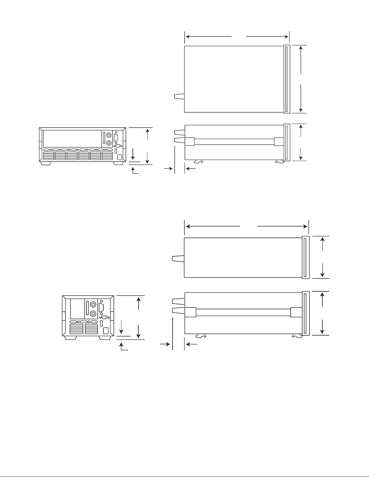
Agilent N3300A
To p
624.8mm
24.6"
425.5mm
16.75"
Agilent N3301A
Rear
190.5mm
12.7mm
190.5mm
7.5"
7.5"
0.5"
50.8mm
2.0"
Side
624.8mm
24.6"
To p
177.8mm
7.0"
213.4mm
8.4"
177.8mm
7.0"
Rear
12.7mm
0.5"
50.8mm
Side
2.0"
9
Page 10

s
myAgilent
www.agilent.com/find/myagilent
A personalized view into the information
most relevant to you.
Agilent Channel Partners
www.agilent.com/find/channelpartners
Get the best of both worlds: Agilent’s
measurement expertise and product
breadth, combined with channel
partner convenience.
Agilent Advantage Services is committed
to your success throughout your equipment’s lifetime. To keep you competitve,
we continually invest in tools and
processes that speed up calibration and
repair and reduce your cost of ownership.
You can also use Infoline Web Services
to manage equipment and services more
effectively. By sharing our measurement
and service expertise, we help you create
the products that change our world.
www.agilent.com/find/advantageservices
Agilent Electronic Measurement Group
DEKRA Certified
ISO 9001:2008
Quality Management SystemQuality Management Sy
www.agilent.com/quality
www.agilent.com
For more information on Agilent
Technologies’ products, applications or
services, please contact your local Agilent
office. The complete list is available at:
www.agilent.com/find/contactus
Americas
Canada (877) 894 4414
Brazil (11) 4197 3600
Mexico 01800 5064 800
United States (800) 829 4444
Asia Pacific
Australia 1 800 629 485
China 800 810 0189
Hong Kong 800 938 693
India 1 800 112 929
Japan 0120 (421) 345
Korea 080 769 0800
Malaysia 1 800 888 848
Singapore 1 800 375 8100
Taiwan 0800 047 866
Other AP Countries (65) 375 8100
Europe & Middle East
Belgium 32 (0) 2 404 93 40
Denmark 45 45 80 12 15
Finland 358 (0) 10 855 2100
France 0825 010 700*
*0.125 €/minute
Germany 49 (0) 7031 464
6333
Ireland 1890 924 204
Israel 972-3-9288-504/544
Italy 39 02 92 60 8484
Netherlands 31 (0) 20 547 2111
Spain 34 (91) 631 3300
Sweden 0200-88 22 55
United Kingdom 44 (0) 118 927
6201
For other unlisted countries:
www.agilent.com/find/contactus
Revised: January 6, 2012
Product specifications and
descriptions in this document subject
to change without notice.
© Agilent Technologies, Inc. 2012
Published in USA, December 5, 2012
5980-0232E
 Loading...