Agilent Technologies 89441A User Manual

Agilent Technologies 89441A Getting Started Guide

Agilent Technologies Part Number 89441-90076

For instruments with firmware version A.08.00 Printed in U.S.A.

This software and documentation is based in part on the Fourth Berkeley Software Distribution under license from The Regents of the University of California. We acknowledge the following individuals and institutions for their role in the development: The Regents of the University of California .

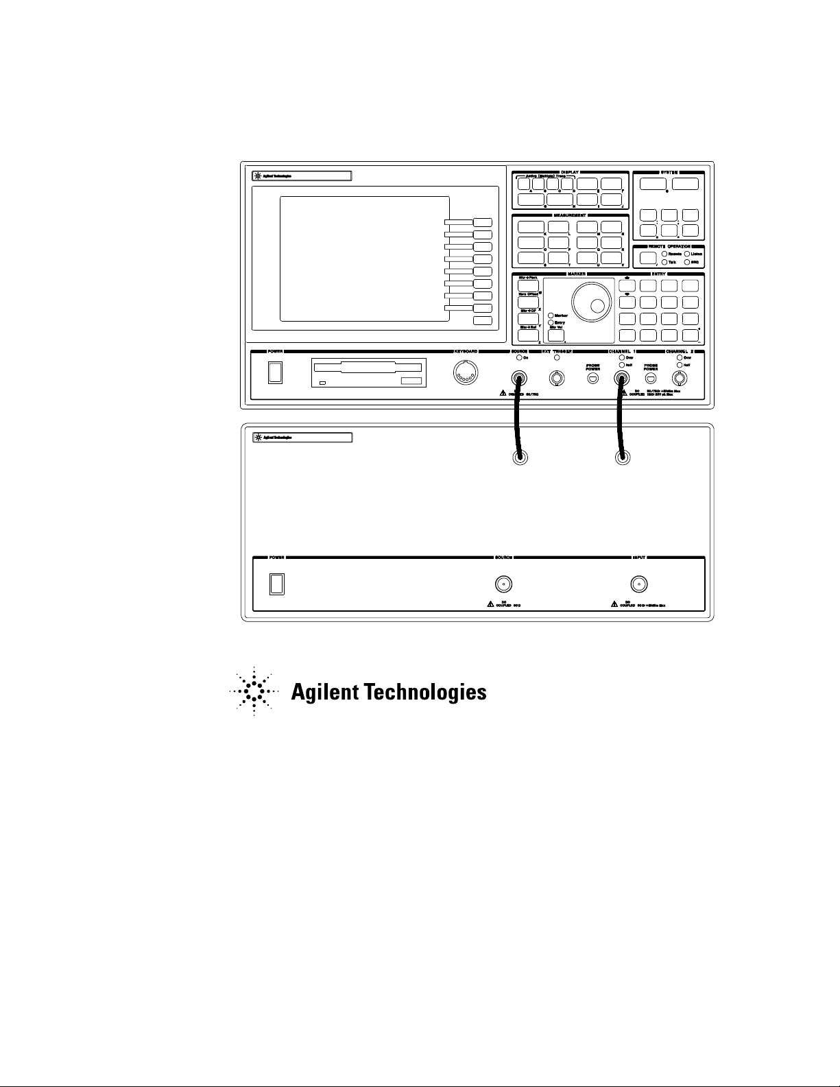
The Analyzer at a Glance

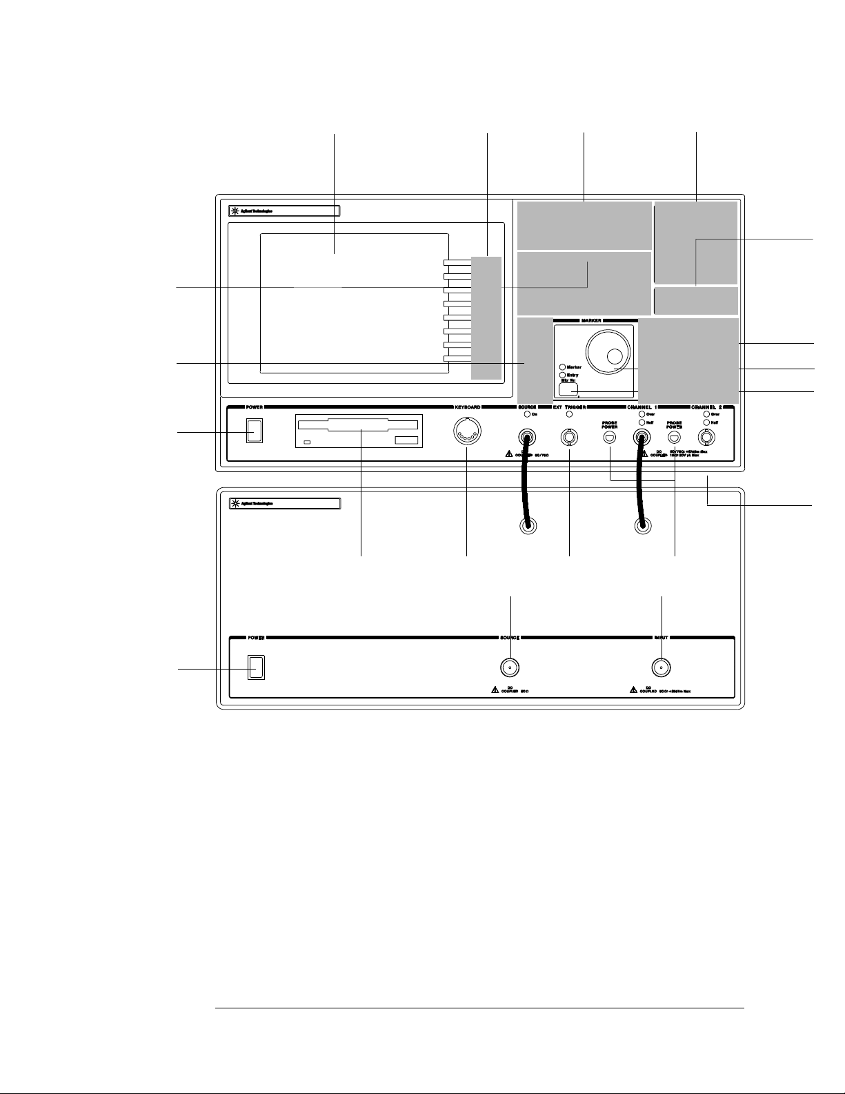
Front Panel

1-A softkey’s function changes as different

menus are displayed. Its current function is determined by the video label to its left, on the analyzer’s screen.

2-The analyzer’s screen is divided into two

main areas. The menu area, a narrow column at the screen’s right edge, displays softkey labels. The data area, the remaining portion of the screen, displays traces and other data.

3-The POWER switch turns the analyzer on

and off.

4-Use a 3.5 inch flexible disk (DS,HD) in this

disk drive to save your work.

11-Use the SYSTEM hardkeys and their

menus to control various system functions (online help, plotting, presetting, and so on).

12-Use the MEASUREMENT hardkeys and

their menus to control the analyzer’s receiver and source, and to specify other measurement parameters.

13-The REMOTE OPERATION hardkey and

LED indicators allow you to set up and monitor the activity of remote devices.

14-Use the MARKER hardkeys and their

menus to control marker positioning and marker functions.

5-The KEYBOARD connector allows you to

attach an optional keyboard to the analyzer. The keyboard is most useful for writing and editing Agilent Instrument BASIC programs.

6- The SOURCE connector routes the

analyzer’s source output to your DUT. If option AY8 (internal RF source) is installed, the conector is a type-N. If option AY8 is not installed, the connector is a BNC. Output impedance is selectable: 50 ohms or 75 ohms with option 1D7 (minimum loss pads).

7-The EXT TRIGGER connector lets you

provide an external trigger for the analyzer.

8-The PROBE POWER connectors provides

power for various Agilent active probes.

9-The INPUT connector routes your test signal

or DUT output to the analyzer’s receiver. Input impedance is selectable: 50 ohms or 75 ohms with option 1D7 (minimum loss pads).

10-Use the DISPLAY hardkeys and their

menus to select and manipulate trace data and to select display options for that data.

15-The knob’s primary purpose is to move a

marker along the trace. But you can also use it to change values during numeric entry, move a cursor during text entry, or select a hypertext link in help topics

16-Use the Marker/Entry key to determine the

knob’s function. With the Marker indicator illuminated the knob moves a marker along the trace. With the Entry indicator illuminated the knob changes numeric entry values.

17-Use the ENTRY hardkeys to change the

value of numeric parameters or to enter numeric characters in text strings.

18-The optional CHANNEL 2 input connector

routes your test signal or DUT output to the analyzer’s receiver. Input impedance is selectable: 50 ohms, 75 ohms, or 1 megohm. For ease of upgrading, the CHANNEL 2 BNC connector is installed even if option AY7 (second input channel) is not installed.

For more details on the front panel, display the online help topic “Front Panel”. See the chapter “Using Online Help” if you are not familiar with using the online help index.

iii

This page left intentionally blank.

Saftey Summary

The following general safety precautions must be observed during all phases of operation of this instrument. Failure to comply with these precautions or with specific warnings elsewhere in this manual violates safety standards of design, manufacture, and intended use of the instrument. Agilent Technologies, Inc. assumes no liability for the customer’s failure to comply with these requirements.

GENERAL

This product is a Safety Class 1 instrument (provided with a protective earth terminal). The protective features of this product may be impaired if it is used in a manner not specified in the operation instructions.

All Light Emitting Diodes (LEDs) used in this product are Class 1 LEDs as per IEC 60825-1.

ENVIRONMENTAL CONDITIONS

This instrument is intended for indoor use in an installation category II, pollution degree 2 environment. It is designed to operate at a maximum relative humidity of 95% and at altitudes of up to 2000 meters. Refer to the specifications tables for the ac mains voltage requirements and ambient operating temperature range.

BEFORE APPLYING POWER

Verify that the product is set to match the available line voltage, the correct fuse is installed, and all safety precautions are taken. Note the instrument’s external markings described under Safety Symbols.

GROUND THE INSTRUMENT

To minimize shock hazard, the instrument chassis and cover must be connected to an electrical protective earth ground. The instrument must be connected to the ac power mains through a grounded power cable, with the ground wire firmly connected to an electrical ground (safety ground) at the power outlet. Any interruption of the protective (grounding) conductor or disconnection of the protective earth terminal will cause a potential shock hazard that could result in personal injury.

FUSES

Only fuses with the required rated current, voltage, and specified type (normal blow, time delay, etc.) should be used. Do not use repaired fuses or short-circuited fuse holders. To do so could cause a shock or fire hazard.

DO NOT OPERATE IN AN EXPLOSIVE ATMOSPHERE

Do not operate the instrument in the presence of flammable gases or fumes.

DO NOT REMOVE THE INSTRUMENT COVER

Operating personnel must not remove instrument covers. Component replacement and internal adjustments must be made only by qualified service personnel.

Instruments that appear damaged or defective should be made inoperative and secured against unintended operation until they can be repaired by qualified service personnel.

WARNING The WARNING sign denotes a hazard. It calls attention to a procedure,

practice, or the like, which, if not correctly performed or adhered to, could result in personal injury. Do not proceed beyond a WARNING sign until the indicated conditions are fully understood and met.

Caution The CAUTION sign denotes a hazard. It calls attention to an operating

procedure, or the like, which, if not correctly performed or adhered to, could result in damage to or destruction of part or all of the product. Do not proceed beyond a CAUTION sign until the indicated conditions are fully understood and met.

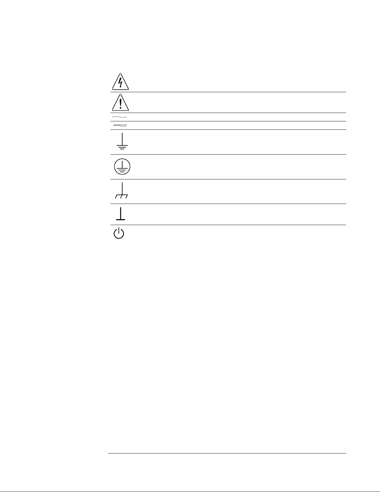
Safety Symbols

Warning, risk of electric shock

Caution, refer to accompanying documents

Alternating current

Both direct and alternating current

Earth (ground) terminal

Protective earth (ground) terminal

Frame or chassis terminal

Terminal is at earth potential.

Standby (supply). Units with this symbol are not completely disconnected from ac mains when

this switch is off

vii

Notation Conventions

Before you use this book, it is important to understand the types of keys on the front panel of the analyzer and how they are denoted in this book.

Hardkeys Hardkeys are front-panel buttons whose functions are always the same.

Hardkeys have a label printed directly on the key. In this book, they are printed like this: [

Hardkey

Softkeys Softkeys are keys whose functions change with the analyzer’s current menu selection. A softkey’s function is indicated by a video label to the left of the key (at the edge of the analyzer’s screen). In this book, softkeys are printed like this: [

Toggle Softkeys Some softkeys toggle through multiple settings for a parameter. Toggle softkeys have a word highlighted (of a different color) in their label. Repeated presses of a toggle softkey changes which word is highlighted with each press of the softkey. In this book, toggle softkey presses are shown with the requested toggle state in bold type as follows: “Press [

Shift Functions In addition to their normal labels, keys with blue lettering also have a shift function. This is similar to shift keys on an pocket calculator or the shift function on a typewriter or computer keyboard. Using a shift function is a two-step process. First, press the blue [ display). Then press the key with the shift function you want to enable. Shift function are printed as two key presses, like this: [

Shift][Shift Function

key name on

]”means“pressthesoftkey [

] key (at this point, the message “shift” appears on the

Shift

]

key name

softkey

] until the selection on is active.”

Numeric Entries Numeric values may be entered by using the numeric keys in the lower right hand ENTRY area of the analyzer front panel. In this book values which are to be entered from these keys are indicted only as numerals in the text, like this: Press 50, [

Ghosted Softkeys A softkey label may be shown in the menu when it is inactive. This occurs when a softkey function is not appropriate for a particular measurement or not available with the current analyzer configuration. To show that a softkey function is not available, the analyzer ‘’ghosts’’ the inactive softkey label. A ghosted softkey appears less bright than a normal softkey. Settings/values may be changed while they are inactive. If this occurs, the new settings are effective when the configuration changes such that the softkey function becomes active.

viii

enter

]

In This Book

This book, “Agilent Technologies 89441A Getting Started Guide”, is designed to help you become comfortable with the Agilent 89441A Vector Signal Analyzers. It provides step-by step examples of how to use this analyzer to perform tasks which you have probably performed with other analyzers. By performing these tasks you will become familiar with many of the basic features—and how those features fit together to perform actual measurements.

This book also contains a chapter to help you prepare the analyzer for use, including instructions for inspecting and installing the analyzer.

To Learn More About the Analyzer

You may need to use other books in the analyzer’s manual set. See the “Documentation Roadmap” at the end of this book to learn what each book contains.

This page left intentionally blank

1 Using Online Help

To learn about online help 1-2

To display help for hardkeys and softkeys 1-3

To display a related help topic 1-4

To select a topic from the help index 1-5

2 Making Simple Noise Measurements

To measure random noise 2-2

To measure band power 2-3

To measure signal to noise ratios 2-4

To measure adjacent-channel power 2-6

3 Using Gating to Characterize a Burst Signal

To Use Time Gating 3-2

4MeasuringRelativePhase

To measure the relative phase of an AM signal 4-2

To measure the relative phase of an PM signal 4-4

5 Characterizing a Filter

To set up a frequency response measurement 5-2

To use the absolute marker 5-4

To use the relative marker 5-5

To use the search marker 5-6

To display phase 5-7

To display coherence 5-8

6 General Tasks

To set up peripherals. 6-2

To print or plot screen contents 6-3

To save data with an internal or RAM disk 6-4

To recall data with an internal or RAM disk 6-5

To format a disk 6-6

To create a math function 6-7

To use a math function 6-8

To display a summary of instrument parameters 6-9

Inspection and Installation

7 Preparing the Analyzer for Use

Preparing the Analyzer for Use 7-2

To do the incoming inspection 7-5

To connect the sections 7-7

To install the analyzer 7-9

To change the IF section’s line-voltage switch 7-10

To change the RF section’s line-voltage switch 7-11

To change the IF section’s fuse 7-12

To change the RF section’s fuse 7-13

To connect the analyzer to a LAN 7-14

To connect the analyzer to a serial device 7-15

To connect the analyzer to a parallel device 7-15

To connect the analyzer to an GPIB device 7-16

To connect the analyzer to an external monitor 7-16

To connect the optional keyboard 7-17

To connect the optional minimum loss pad 7-18

To clean the screen 7-19

To store the analyzer 7-19

To transport the analyzer 7-20

If the IF section will not power up 7-21

If the RF section will not power up 7-22

If the analyzer’s stop frequency is 10 MHz 7-23

Index

Documentation Road Map

Need Assistance

xii

Using Online Help

You can learn about your analyzer from online help which is built right into the instrument and is available to you any time you use the analyzer. This section shows you how to use online help to learn about specific keys or topics. You can use online help in conjunction with other documentation to learn about your analyzer in depth, or you can refresh your memory for keys you seldom use. You can use online help while working with your analyzer since online help does not alter the analyzer setup.

1-1

Using Online Help

To learn about online help

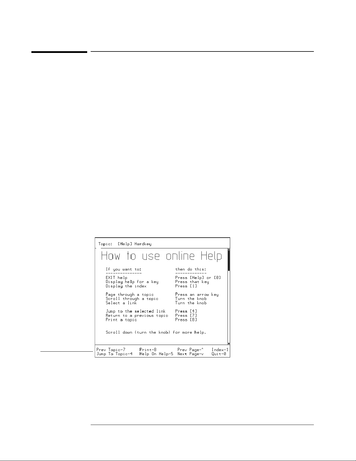
1 Enter the online help system:

Press [

2 Display online help for the [

Press [

3 Use the knob or the up-arrow or down-arrow keys to move through the pages. 4 Quit online help:

Press [ or Press [

Take a few moments to read the help overview. It’s only five pages long, and it includes descriptions of advanced features like the index and cross-reference “links” that can help you locate the information you need more quickly.

When you enter the help system it displays help on the last key you pressed. If you have just turned on the analyzer online help for the [

Help

] on the numeric keypad.

Help

] on the keypad.

] hardkey:

] key is displayed.

Help

This legend shows which numeric keys access online help features

When you quit help, the analyzer restores the display and menu that was displayed before you enabled help. Using online help does not alter your measurement setup.

1-2

Using Online Help

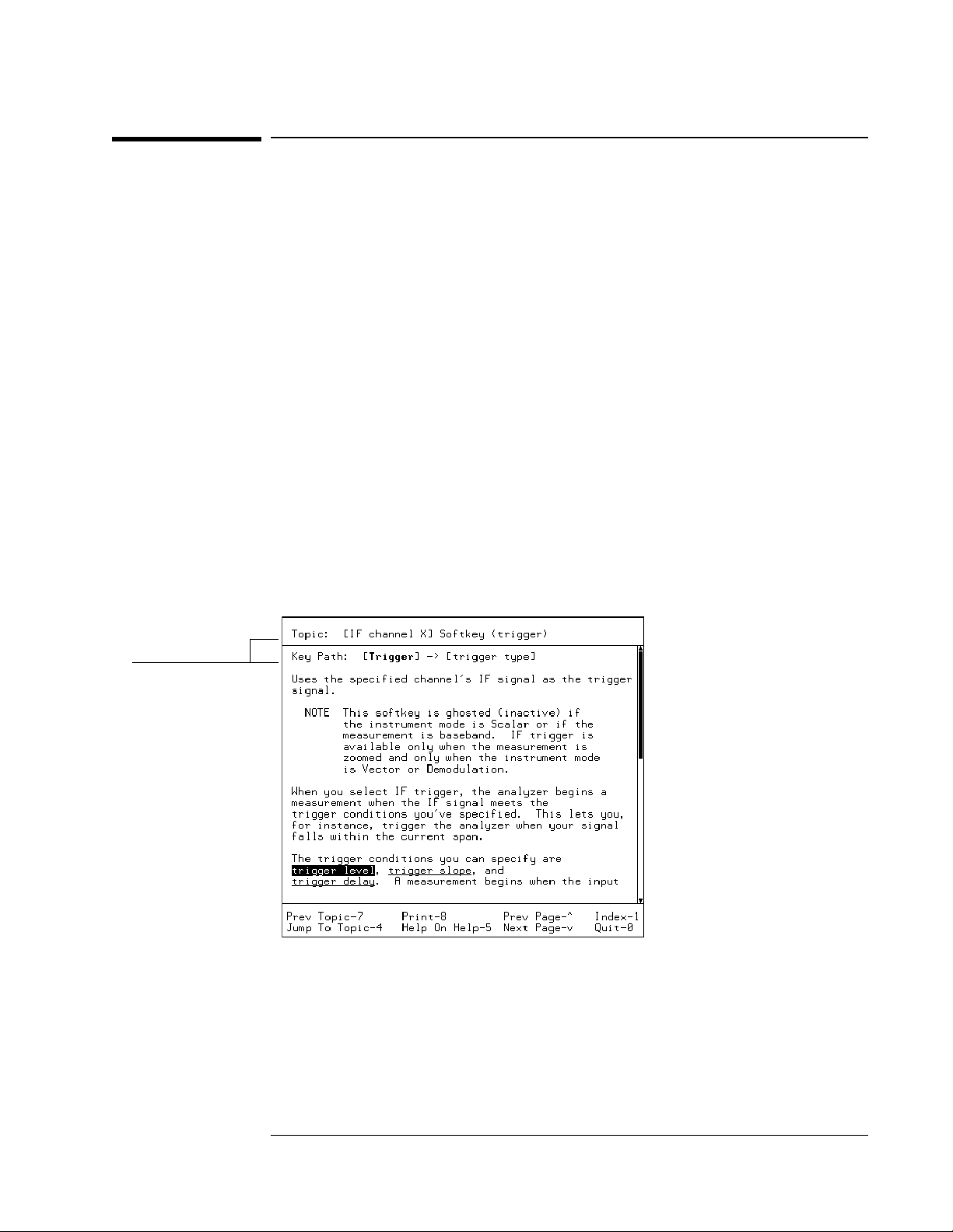
To display help for hardkeys and softkeys

This example displays topics related to triggering.

1 Enter the online help system:

Press [

2 Display help for a hardkey:

Press [

3 Use the knob or the up and down arrow keys to page through the topic. 4 Select a softkey topic:

Press [

5 Quit online help:

Press [ or Press [

Pressing [ other key when help is enabled, the analyzer displays a help topic describing the key’s function. For help on the preset state, select “Preset hardkey” from the help index (you will learn how to do this later in this section) or press [ then [

Help

Trigger

trigger type

Help

] on the keypad.

Help

], [

IF channel 1

]

] always returns the analyzer to its preset state. If you press any

Preset

]

These lines show the name of the selected softkey and the path to its hardkey

1-3

Using Online Help

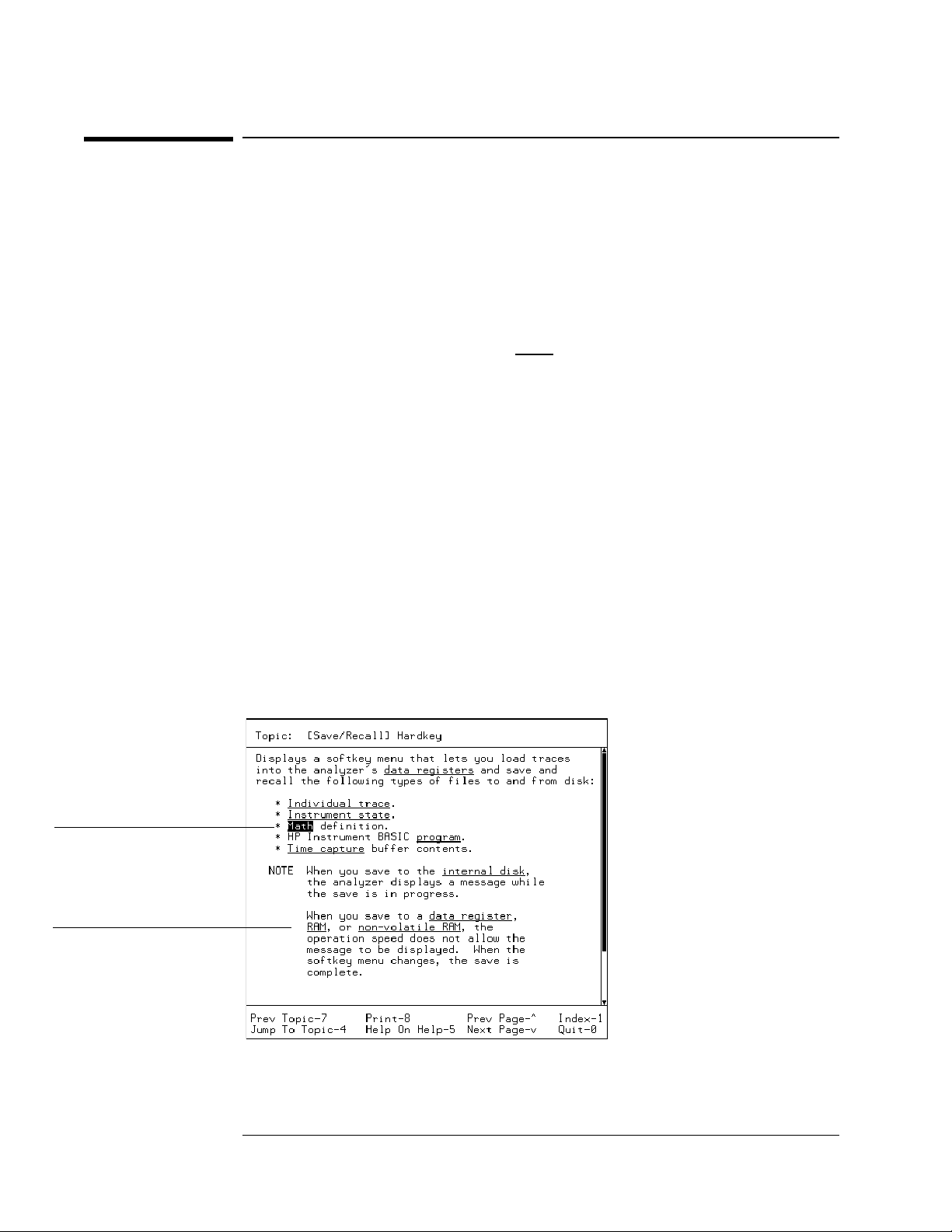
To display a related help topic

This example displays topics related to saving and recalling.

1 Enter the online help system:

Press [

2 Display help for a hardkey:

Press [

3 Scroll with the knob to highlight the Math topic. 4 Select that topic:

Press [

5 Return to previous topics:

Press [

6 Quit online help:

Press [ On a given screen full of online help text, there may be several special words (or

phrases) that are linked to related topics. Most of these words are underlined to identify them as links, but one is highlighted to identify it as the currently-selected link. The knob allows you to select a different link by moving the highlighting from one link to the next. Once you’ve selected the link you want, press [

Help

Save/Recall

Help

] on the keypad to display the related topic.

The highlighted link shows what topic is displayed if you press 4

Underlined links show other topics available from this online help topic

You can follow links through as many as 20 topics and still return to the original topic. Just press [

] one time for each link you followed, and you’ll return to the

original topic via all of the related topics you displayed.

1-4

Using Online Help

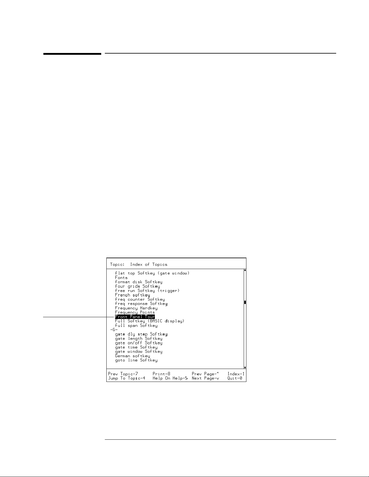
To select a topic from the help index

1 Enter the online help system:

Press [

2 Display the index:

Press [

3 Turn the knob to select the topic you want help on

for faster paging press and hold the up-arrow or down-arrow keys then use the knob to select a topic.

4 Display the topic:

Press [

5 Quit online help:

Press [ or Press [

The help index contains an alphabetical listing of all help topics. Most topics listed in the index describe the hardkeys and softkeys, but some are of a more general nature. These more general topics are only available via the index or via “links” from related topics. An example appears below–the “Front Panel Tour” topic is only available through the index or the “links”, not by pressing any hardkey or softkey.

Help

You can select any topic in the index by scrolling to highlight it then pressing 4

1-5

Making Simple Noise Measurements

This chapter shows you how to make typical noise measurements. In this example, we will be making random noise, band power noise, and signal to noise measurements.

2-1

Making Simple Noise Measurements

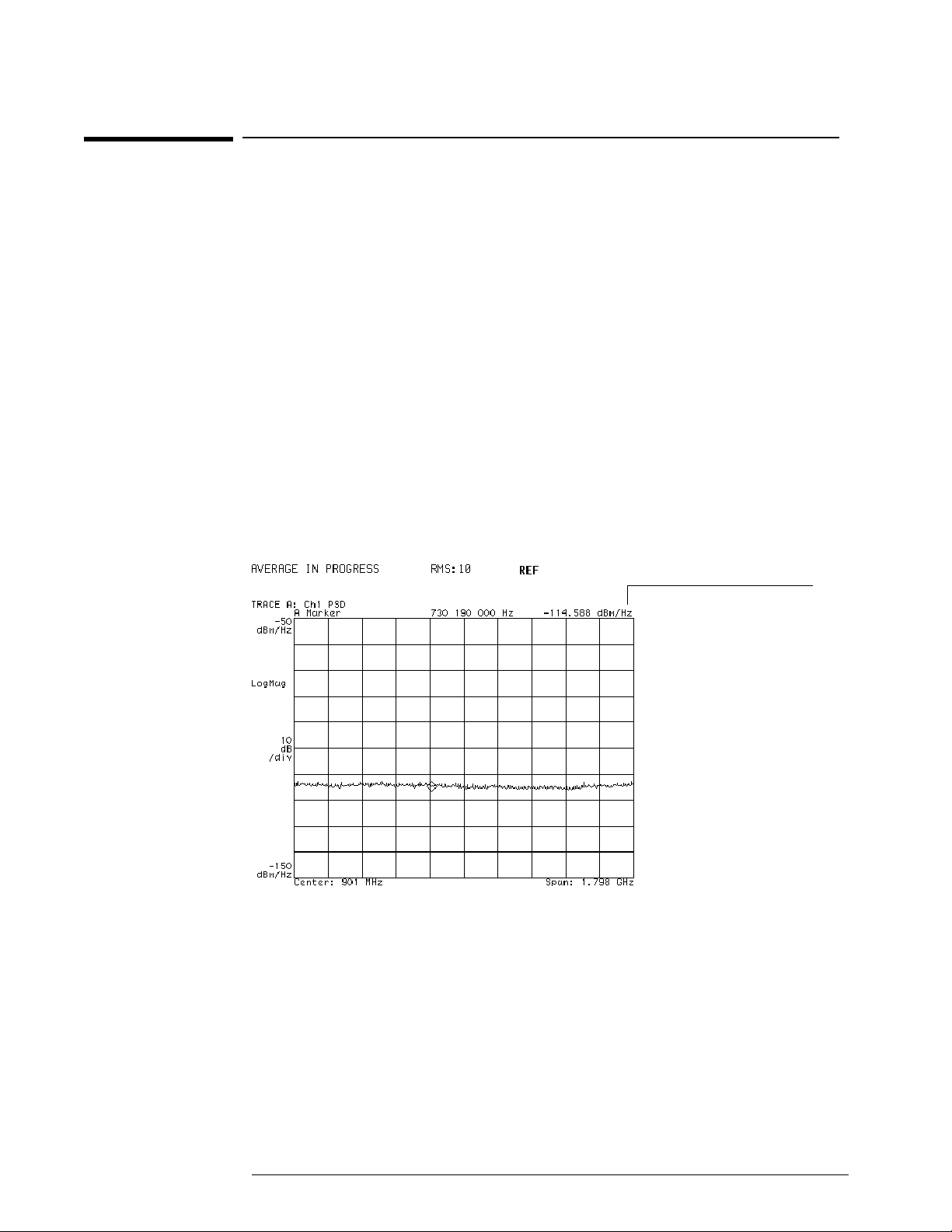
To measure random noise

1 Initialize the analyzer:

Press [

2 Select a power spectral density measurement:

Press [

3 Turn on averaging:

Press [

4 Start an averaged measurement:

Press [

5 Use the knob to move the marker along the trace.

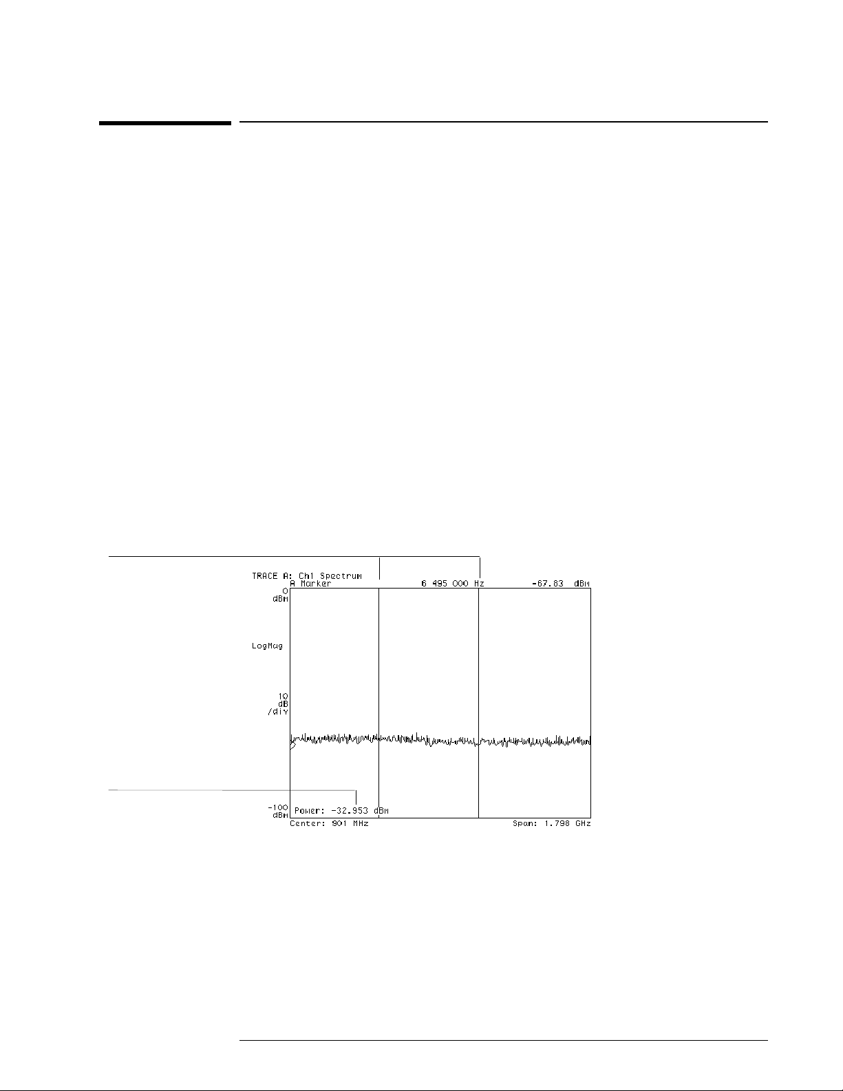
The display should be similar to the one shown below.

To learn more about the choices you make in this measurement, display online help for the various keys used (see “Using Online Help” if you are not familiar with how to do this).

Preset

Measurement Data

], [

Average

Meas Restart

average on

], [

](selectch1 with a 2-channel analyzer).

PSD

Normalized noise measurement

In this example you are measuring the noise-power of the analyzer’s noise floor. The displayed marker value reflects noise-power normalized to a 1-Hz bandwidth.

2-2

Making Simple Noise Measurements

To measure band power

1 Initialize the analyzer:

Press [

2 Turn on averaging:

Press [

3 Start an averaged measurement:

Press [

4 Turn on the band power markers:

Press [ Press [ Press [

5 Change the width of the band:

Press [ then use the knob to move the marker to the desired location. Press [ then use the knob to move the marker to the desired location.

The display should similar to the one below. The grid lines have been turned off to highlight the band power markers.

Preset

Average

Meas Restart

Marker Function ResBW/Window Marker Function

band right

band left

], [

average on

], [

Marker|Entry

], [

band power markers

], [

detector

], [

band power markers

], [

sample

], [

band pwr mkr on

]

], [

band power

]

Band power markers

Band power magnitude

In this example you are measuring the power of the analyzer’s noise floor within a defined band. The value displayed in the lower left corner of the display reflects the total power within the frequency band encompassed by the markers. The grid lines have been turned off to highlight the band power markers.

2-3

Making Simple Noise Measurements

To measure signal to noise ratios

1 Select the baseband receiver mode and initialize the analyzer:

Press [ Press [

Instrument Mode][receiver][RF section (0-10 MHz)

Preset

2 Supply a signal from the internal source:

Connect the SOURCE output to the INPUT with a BNC cable. Press [

Source

], [

source on

], [

sine freq

], 5, [

3 Place the marker on the signal peak:

Press [ or Press [

Marker⇒

Shift

], [

marker to peak

Marker

]

4 Select video averaging:

Press [

Average

], [

average on

]

5 Turn on the carrier-to-noise marker:

Press [

6 Press [

Marker Function

Marker|Entry

Rotate the knob to move the measurement band from the signal to a noise area.

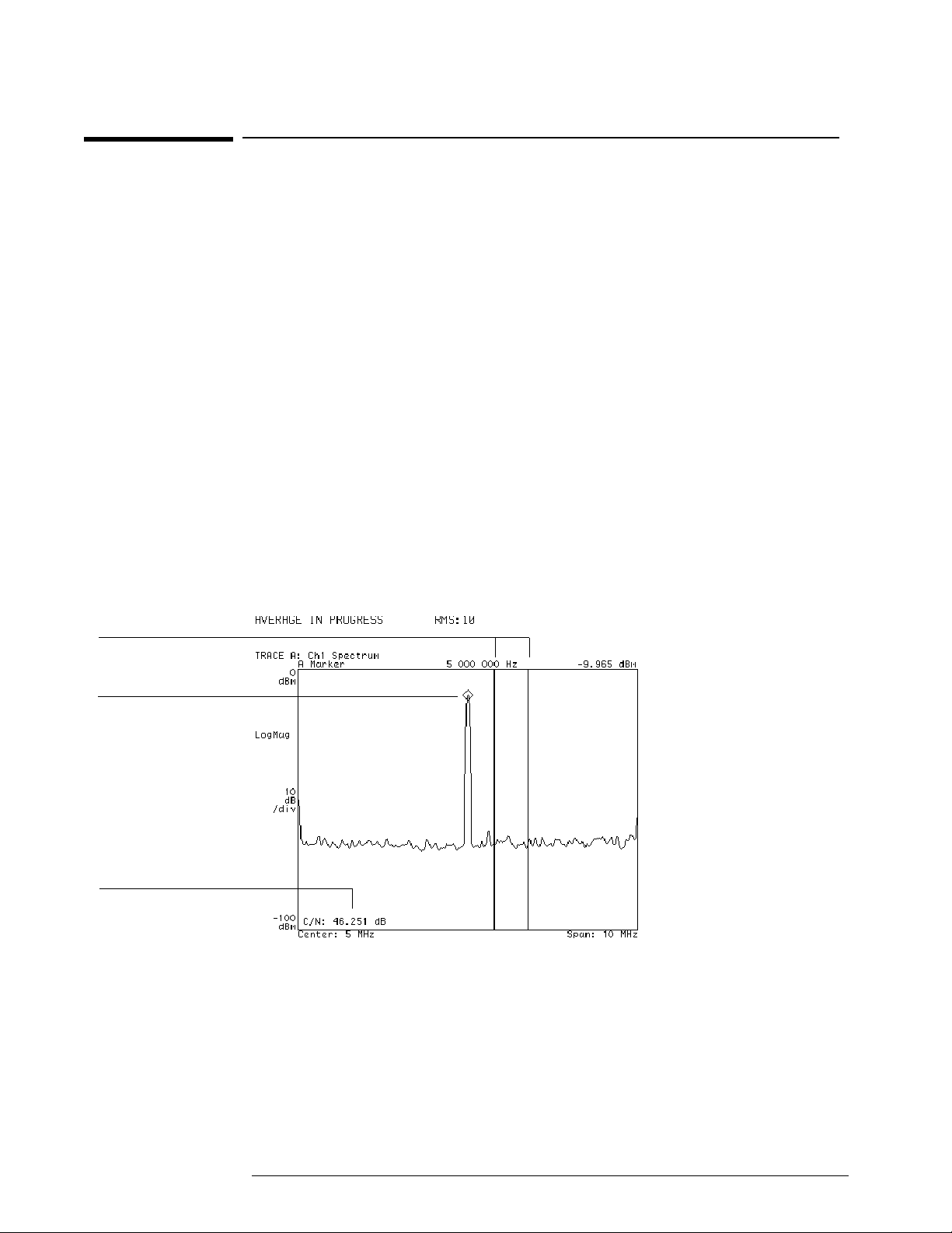
The display should appear as below. The grid lines have been turned off to highlight the band power markers.

], [

band power markers

]

], [

]

MHz

band pwr mkr on

], [

power ratio

C/N

Measured noise band

The diamond shaped marker provides a reference point

Carrier to noise ratio

The value indicated in the lower left corner of the display reflects the difference between the marker level at the carrier peak and the total noise within the band markers.

2-4

Measured noise band

The diamond shaped marker provides a reference point

Making Simple Noise Measurements

7 Change to a normalized noise measurement:

Toggle to [

power ratio C/No

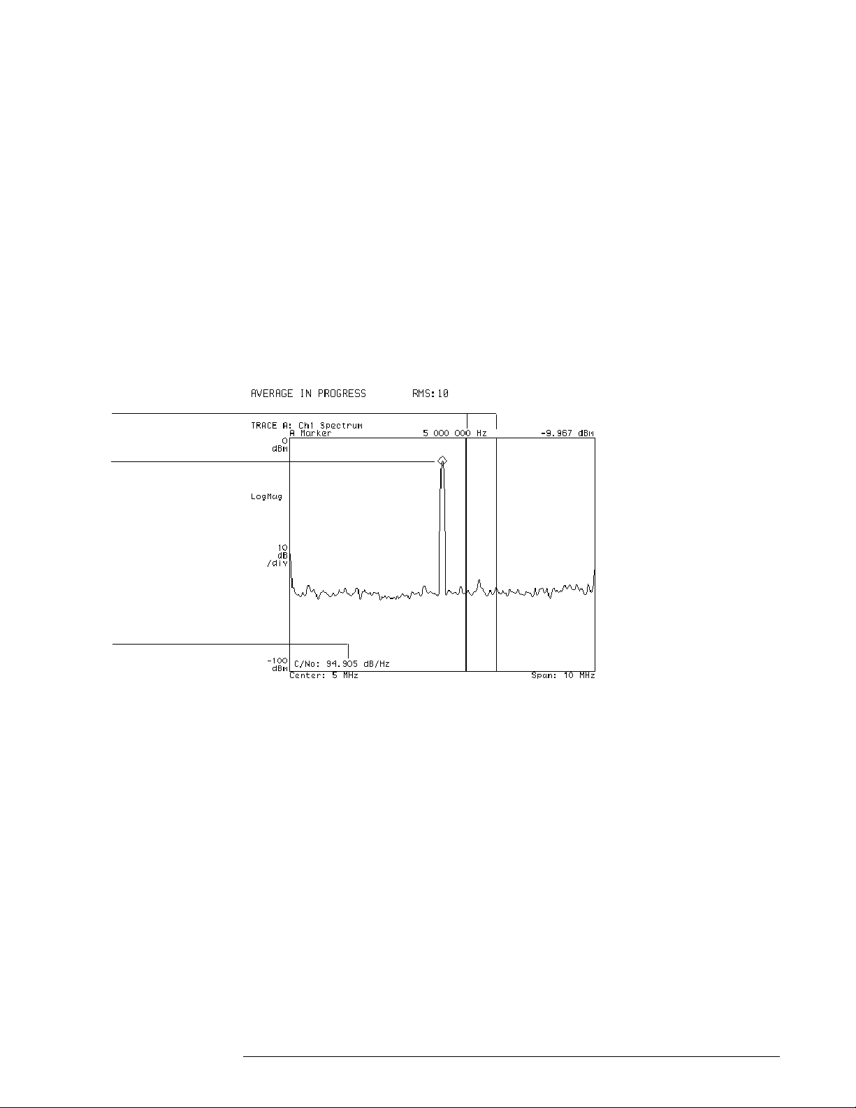
The display should appear as below. The grid lines have been turned off to highlight the band power markers.

The carrier-to-noise and carrier-to-normalized-noise marker measurements require that the standard (diamond shaped) marker be on the signal peak as a reference. If the marker is not on, the displayed value will only reflect the noise level.

Step 3 above illustrates that there are two ways to perform certain actions—by using the hardkey/softkey sequence or by using the short-cut shift/hardkey sequence.

]

Carrier-to-noise ratio normalized to one Hertz

Now the value indicated in the lower left corner of the display reflects the difference between the marker level at the carrier peak and the noise-power within the band markers normalized to one Hertz bandwidth.

You can perform band power measurements in either Vector or Scalar Mode. If you use Scalar mode and you have selected a combination of resolution bandwidth, window type, and number of frequency points such that the analyzer implements the detector, the analyzer will prompt you to select the sample detector in order to calculate the band power accurately.

2-5

Using Gating to Characterize a Burst Signal

This chapter uses the time gating feature to analyze a multi-burst signal which is provided on the Signals Disk which accompanies the analyzer’s Operator’s Guide. Time gating allows you to isolate a portion of a time record for further viewing and analysis. For more details on time gating concepts see “Gating Concepts” in the Operator’s Guide.

3-1

Using Gating to Characterize a Burst Signal

To Use Time Gating

First we’ll look at the spectrum of the signal and see that three components exist. Then we’ll look at the time display of the burst signal and analyze each burst separately to determine which spectral components exist in each burst.

1 Select the baseband receiver mode and initialize the analyzer:

Press [ Press [

Instrument Mode][receiver][RF section (0-10 MHz)

Preset

2 Load the source signal file BURST.DAT into data register D3:

Insert the Signals Disk in the analyzer’s disk drive. Press [ Press [

Save/Recall

Return

], [

default disk

] (bottom softkey), [

], [

internal disk

catalog on

Rotate the knob until the file BURST.DAT is highlighted. Press [

recall trace

], [

from file into D3

], [

enter

3 Connect the SOURCE output to the INPUT with a BNC cable. 4 Turn on the source and select arbitrary signal D3:

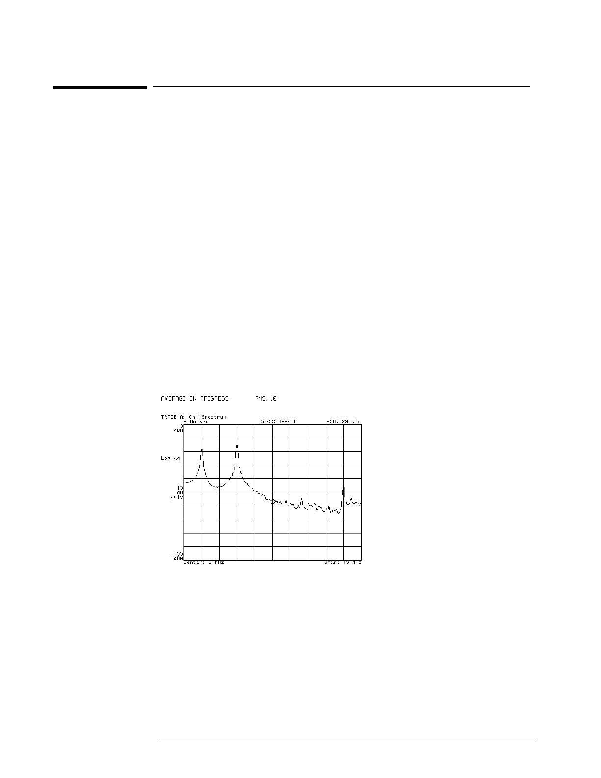
Press [ Press [ The display should now appear as shown below.

Source Average

], [

source on

average on

], [

source type

], [

arb data reg

] to select the internal disk drive.

] to display the files on the disk.

], [D3], [

Return

], [

arbitrary

The spectrum with averaging turned on. Note existence of three components.

3-2

Using Gating to Characterize a Burst Signal

5 Configure the display and the measurement:

Press [ Press [ Press [ Press [ Press [

], [

Display

], [

Measurement Data

Ref Lvl/Scale

], [

Trigger Time

], [

trigger type

main length

2grids

], [

more display setup

], [ ], 50, [mV].

Yperdiv

], [

internal source

], 32, [us].

main time

], [

grids off

] (toggle to ch1 on a 2-channel analyzer).

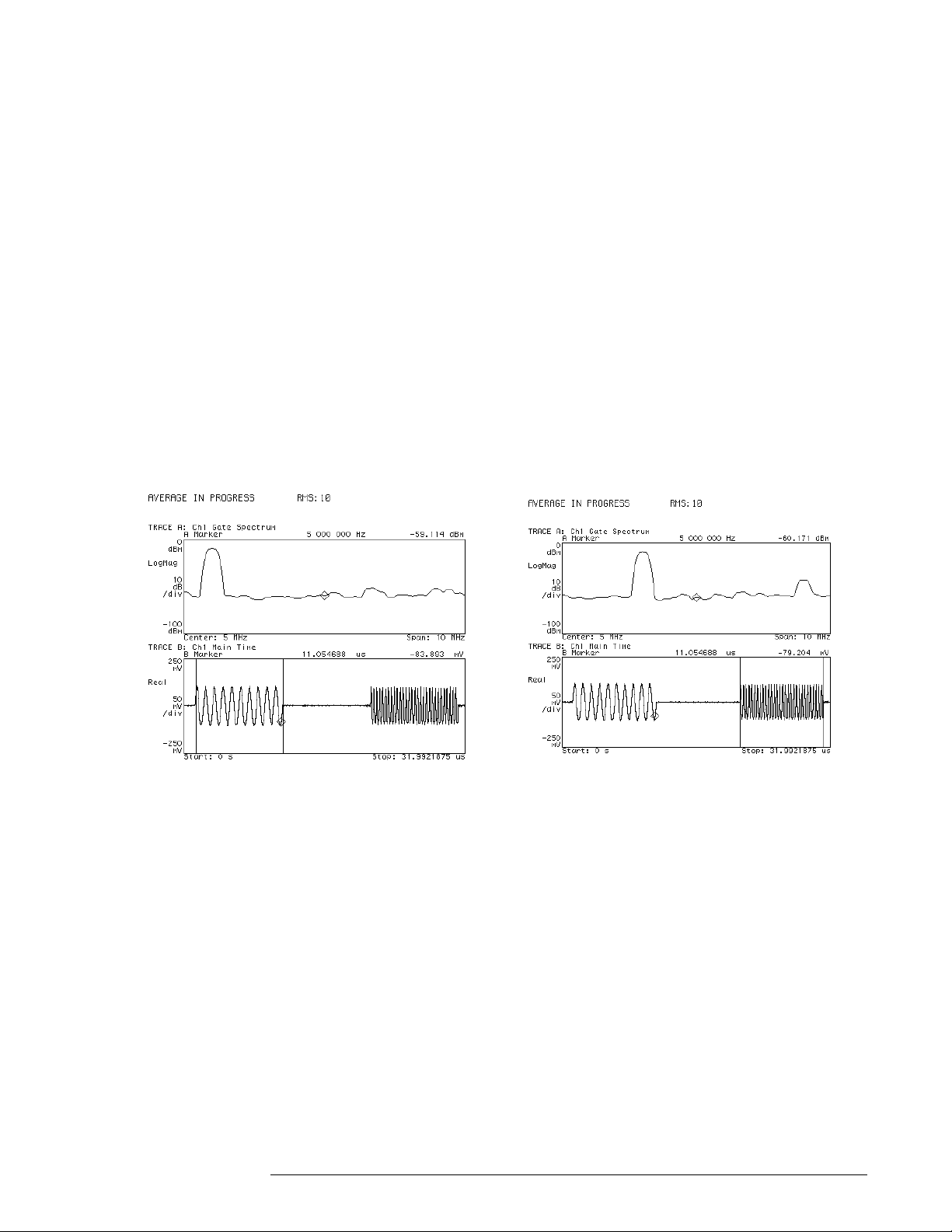
6 Set up the time gating and examine the first burst:

Press [ Press [ Rotate the knob until the gate is at each end of the first burst signal. The display should now appear as shown to the left below.

], [

Time

ch1 gate dly

gate on

], [

Marker|Entry

], [

gate length

], 10, [us].

]

7 Examine the second burst:

Rotate the knob until the gate is at each end of the second burst signal. The display should now appear as shown to the right below.

Note that the [

] menu must be displayed, the [

Time

gate delay

] softkey active, and

theknobintheEntrymodetomovethegatebyturningtheknob.

Spectrum (top trace) of the burst is derived by gating the time signal (bottom trace). The gate’s delay and length are selected to encompass the burst signal (vertical markers show gate position). Note existence of the first spectral component in the left display and the existence of the other two components in the right display.

3-3

Measuring Relative Phase

This section shows you how to make typical relative phase measurements on modulated carrier signals. In this example, you measure the phase of sidebands on AM and PM signals relative to the carrier. The test signals are provided on the Signals Disk which accompanies the analyzer’s Operator’s Guide.

4-1

Measuring Relative Phase

To measure the relative phase of an AM signal

1 Select the baseband receiver mode and initialize the analyzer:

Press [ Press [

Instrument Mode][receiver][RF section (0-10 MHz)

Preset

2 Load AM and PM signals from the Signals Disk into registers and play the AM

signal through the source:

Insert the Signals Disk in the internal disk drive. Use the BNC cable to connect the SOURCE output to the INPUT. Press [ Press [

Save/Recall

], [

Return

], [

default disk

catalog on

], [

internal disk

]. Rotate the knob to highlight AMSIG.DAT Press [

recall trace

], [

from file into D1

], [

enter

]. Rotate the knob to highlight PMSIG.DAT Press [ Press [

from file into D2][enter

], [

Source

source on

], [

source type

], [

arbitrary

3 Configure the measurement and display:

Press [ Press [ Press [

Frequency Trigger Sweep

], [

span

trigger type

single

], 150, [

], [

internal source

kHz

4 Activate a different trace as a phase display:

Press [ Press [B], [ Press [

], [

Display

Data Format

2grids

Measurement Data

], [

phase wrap

], [

](selectch1 with a 2-channel analyzer),

spectrum

]

5 Start a single sweep:

Press [

Pause|Single

4-2

Measuring Relative Phase

6 Activate two traces:

Press [

], [A](twoActiveTraceLEDsarenowturnedon)

Shift

7 Turn on marker coupling and zero the offset marker on the carrier:

Press [ Press [ Press [

Marker

], [

Shift

], [

Shift

], [

couple mkrs on

Marker

Marker⇒

] to place the marker on the carrier peak,

] to zero the offset marker.

8 Use the search marker to measure the phase of the two largest sidebands

relative to the carrier:

Press [ Press [

Marker Search

next peak

], [

next peak

], and note the phase displayed for the lower trace.

] again and note the phase.

The phase values vary with each sweep but for an AM signal the average phase of the sidebands is equal to the carrier phase.

4-3

Measuring Relative Phase

To measure the relative phase of an PM signal

Continue from “To measure the relative phase of an AM signal.”

1 Replace the arbitrary source AM signal with the PM signal in register D2:

Press [

2 Start a single sweep:

Press [

3 Zero the offset marker on the carrier:

Press [ Press [

4 Use the search marker to measure the phase of the two largest sidebands

relative to the carrier:

Press [ Press [

], [

Source

Pause|Single

Shift Shift

Marker Search

next peak

source type

], [

Marker

], [

Marker⇒

] again and note the phase.

], [

]

next peak

arb data reg

], [D2].

] and note the phase displayed for the lower trace.

The phase values vary with each sweep but for a PM signal the average phase of the two sidebands is equal to –90 degrees from the carrier.

4-4

Characterizing a Filter

This section shows you how to make a typical network measurement. In this example, we will be characterizing a 4.5 MHz bandpass filter.

5-1

Characterizing a Filter

To set up a frequency response measurement

Note: This measurement can only be performed with a 2-channel analyzer—you must

have option AY7.

You must use the source output and the channel 1 and channel 2 inputs on the IF section for network measurements.

1 Using a BNC “T” adapter or power splitter and BNC cables, connect the

analyzer’s SOURCE to the CHANNEL 1 input directly and to the CHANNEL 2 input through a filter as shown in the illustration below.

2 Select the IF baseband receiver mode and initialize the analyzer:

Press [ Press [

Instrument Mode][receiver][IF section (0-10 MHz)

Preset

3 Configure the analyzer to make two-channel frequency response measurements:

Press [

Measurement Data

], [

freq response

5-2

Characterizing a Filter

4 Configure the source and measurement for a frequency response measurement:

Press [ Press [ Press [ Press [

], [

Source

source type Return level

source on

], [

periodic chirp

], (bottom softkey)

], .5, [ Vrms].

Press [ Press [

Press [

Press [ Press [ Press [

Press [

Res Bw/Window

main window

], [

Range

], [

Average

num averages average type

Auto Scale

], [

uniform

channel both

average on

], 50, [

], [

rms (video)

rbw mode arb

], [

ch* single range up-down

]

enter

5 Start an averaged measurement:

Press [

Meas Restart

The display should appear similar to that shown below. To learn more about the choices you make in this measurement, display online help for the various keys used (see “Using Online Help” if you are not familiar with how to do this).

Note the distinction between selecting the range (the sensitivity of the analyzer’s input circuitry) and selecting the scale (the position of the data on the display).

Frequency response data displays the output of a device-under-test divided by the input

5-3

Characterizing a Filter

To use the absolute marker

Continue from “To set up a frequency response measurement.”

1 Move the marker to the largest part of the frequency response trace:

Press [

Marker

⇒], [

marker to peak

or Press [

Shift

], [

Marker

]

2 Move the marker with the knob to view the absolute gain/loss of this particular

filter network at different frequencies.

Note that there are two ways to perform some functions. In this example you may move the marker to the highest point on the trace by selecting the function in a softkey menu or by using a shift function.

The frequency and amplitude of the trace at the marker location are shown at the top of the display

The marker reflects the absolute amplitude and frequency

5-4

Characterizing a Filter

To use the relative marker

Continue from “To set up a frequency response measurement” or from “Using theabsolutemarker.”

1 Move the marker to the largest part of the frequency response trace if it is not

already there:

Press [

Shift

], [

2 Establish the reference point for the relative (offset) marker:

Press [ or

Press [

Marker

], [

Shift

], [

3 Move the marker with the knob to view the relative gain/loss of this particular

filter at different frequencies.

The offset marker allows you to establish a reference point with the square-shaped marker. As you move diamond-shaped marker, the value displayed by the marker readout reflects the difference between the reference point and the marker.

Marker

zero offset

Marker

]

⇒]

The marker frequency and amplitude reflect the value of the diamond-shaped marker relative to the offset (square) marker

The marker reflects the amplitude and frequency relative to the reference point

5-5

Characterizing a Filter

To use the search marker

Complete “To set up a frequency response measurement” or continue from one of the previous marker measurements.

1 Move the marker to the largest part of the frequency response trace if it is not

already there:

Press [

Shift

], [

2 Activate and zero the offset marker if it is not already activated:

Press [

Shift

], [

3 Define the search target level and perform a search:

Press [ Press [ Press [

The search marker allows you to quickly find a target value. When the offset markerisactivatedthetargetvalueisrelativetothereferencepoint.

Marker Search

search target search right

Marker

], −6, [

], [

search left

⇒].

], [

search setup

With the offset marker activated, the search marker indicates the point on the trace which is separated from the offset marker by the target value

The search marker finds a Y-axis value with reference to a target value

5-6

Characterizing a Filter

To display phase

Complete “To set up a frequency response measurement” or continue from one of the previous marker measurements.

1 Display a second trace:

Press [

2 Activate the second trace and define it as a frequency response measurement:

Press [

3 Specify phase data for the second trace:

Press [

4 Couple the markers on traces A and B:

Press [

5 Move the markers with the knob to determine phase with respect to frequency

response.

6 Overlap the two traces:

Press [ Press [

], [

Display

], [

Measurement Data

Data Format

], [

Marker

], [A].

Shift Display][single grid

2grids

], [

phase wrap

couple mkrs on

], [

frequency response

In this example, note that a trace which is displayed is not necessarily active (capable of being configured). You must specifically activate a displayed trace in order to change its configuration. For example, if you have chosen the relative marker in one trace then couple the markers, the marker on the second trace will be absolute, rather than relative, unless you activate the second trace and select the relative marker.

Coupling the markers on two traces lets you compare values at the same frequency

5-7

Characterizing a Filter

To display coherence

Complete “To set up a frequency response measurement” or continue from one of the previous measurements.

1 Display a second trace:

Press [

2 Activate the second trace and select a coherence measurement:

Press [ [

Measurement Data

Display

], [

2grids

Data Format

], [

more choices

], [

magnitude linear

], [

coherence

Coherence indicates the statistical validity of a frequency response measurement

5-8

General Tasks

This chapter shows you how to perform various common tasks. These include setting up and using peripherals and defining and using math functions.

6-1

General Tasks

To set up peripherals.

You may connect peripherals to three ports—one GPIB port, one serial port, and one parallel port. GPIB peripherals may include printers, plotters, and external disk drives. Supported serial devices are plotters and printers. Certain printers are parallel devices.

1 Connect the ports of your peripheral and analyzer with the correct cables. See

“Preparing the Analyzer for Use” for information on physical connections.

2 Turn on the peripherals. 3 Set up GPIB peripherals:

Determine the address of the peripheral from your peripheral’s documentation Use this as <num> below. On the analyzer, press [ Press the softkey corresponding to your device type. Press <num>, [ Repeat this step for each GPIB peripheral.

enter

Local/setup

], [

peripheral addresses

4 Set up serial peripherals:

Refer to your serial device’s documentation to select correct setup parameters. Press [

Serial 1 setup

] and enter the correct parameters.

Note that the parallel interface requires no special setup.

Display online help for more details on setup and parameter choices.

6-2

To print or plot screen contents

1 Set up your printer or plotter if you haven’t already done so. 2 Select the output format and device type:

Press [ Press [

Plot/Print

device defaults

3 Select the type of output port:

Press [ and select the port to which your printer or plotter is attached.

4 Press [

Plot/Print

Local/Setup

], [

output fmt

] and select the desired format.

] and select a device if you want other than the default.

], [

]

output to

system controller

General Tasks

5 Press [

Plot/Print

], [

start plot/print

]

Theanalyzerisonlyabletoinitiateprintingorplottingifitisattachedtoa printer or plotter and is designated as the system controller. If you haven’t already set up your printer or plotter, see “To set up peripherals.” All of the screen’s contents, except the softkey labels, are printed when you complete this task.

You may select various parameters under the [

plot item

]and[

plot/print setup

] softkeys depending on your particular peripheral. To learn more about these parameters, display online help for the relevant softkeys.

You must use the PLOT/PRINT menu to select the correct type of device and port before starting a plot or print of the screen contents.

With a plotter, you can elect to plot portions of the display

You can control certain device options, depending on your output device

6-3

General Tasks

To save data with an internal or RAM disk

You may save trace data, instrument states, trace math functions, instrument BASIC programs, and time-capture buffers.

1 Select the default disk:

Press [ Press [

2 Press [

Save/Recall

nonvolatile RAM disk

Return

3 Press the softkey that matches the type of data you want to save. 4 Enter the file name if you have chosen to save to a file:

Use the hardkeys (which have now been remapped to represent the symbols etched to the lower right of them), softkeys, knob, and numeric keys to type in a file name.

5 Press [

For more information on the softkeys and parameter choices, display online help.

enter

], [

default disk

]

], [

volatile RAM disk

]or [

internal disk

]

If you are using the internal disk drive, you must insert a formatted 3.5-inch flexible disk into the analyzer’s internal disk drive. If you want to save data but the disk has not been previously formatted see “To format a disk.”

6-4

General Tasks

To recall data with an internal or RAM disk

You may recall trace data, instrument states, trace math functions, instrument BASIC programs, and time-capture buffers.

1 Select the default disk:

Press [ Press [

2 Press [

Save/Recall

nonvolatile RAM disk

Return

3 To easily recall a file you may press [

stored on the disk then use the knob to scroll to the desired file.

4 Press the softkey that matches the type of data you want to recall (then select a

storage register if you are recalling a trace).

5 If you have not selected a file name from the catalog, enter the file name:

Use the hardkeys (which have now been remapped to represent the symbols etched to the lower right of them), softkeys, knob, and numeric keys to type in a file name.

6 Press [

enter

], [

default disk

]

], [

volatile RAM disk

]or [

catalog on

internal disk

]

] to display the names of files

For more information on the softkeys and parameter choices, display online help.

6-5

General Tasks

To format a disk

1 Select the disk drive you want to format:

Press [ Press the softkey corresponding to the disk drive you want to format.

2 Press [

Select appropriate parameters for your disk drive (disk type, interleave etc.).

3 Press [

You may format 3.5-inch disks in the internal disk drive. They must be double-sided, high-density flexible disks that are not write-protected.

The analyzer may take a few minutes to format a disk (depending on the type of disk) and is unavailable for other tasks during that time.

Disk Utility

Return

perform format

Caution You can damage both the disk and the drive if you attempt to eject a disk when

the “Format disk in progress” message is displayed or when the disk’s “busy” light is on.

], [

default disk

format disk

], [

proceed

6-6

To create a math function

In this section you learn how to create a math function which inverts a signal.

1 Initialize the analyzer:

Press [

2 Define a constant:

Press [ Press [

3 Define a math function:

Press [ Press [

A math function remains in memory through a Preset but will be erased when you power down the analyzer. If you want to preserve the math function for future use, save it in the non-volatile RAM or on an internal disk.

Preset

Math

real part

Math

constant

], [

]

define constant

], 1, [

enter

]

define F1

], [K1], [/], [

], [

meas data

define K1

imag part

]

], 0, [

], [

spectrum

enter

], [

enter

General Tasks

You can create up to 6 functions and 5 constants

6-7

General Tasks

To use a math function

In this section you learn how to apply a a math function to a signal. This task assumes that you have completed “To create a math function.”

1 Initialize the analyzer:

Press [

2 Provide an averaged signal from the internal source:

Press [

3 Apply the inversion math function you created to this signal:

Press [

4 Press [

]

Preset

], [

Source

Measurement Data

Auto Scale

source on

], [

Average

math func

], [

average on

], [F1].

A user-created math function is applied to a signal

6-8

To display a summary of instrument parameters

General Tasks

1 Press [ 2

Press [

These summaries reflect the current states of important measurement, input, and source parameters. You may use these summaries to:

You will note that the contents of the measurement state differ depending on the instrument mode. This reflects the fact that some parameters are not used for a particular instrument mode.

View State

measurement state

quickly check the current setup

document the setup (The list can be printed or plotted.)

]or[input/source state].

State summaries provide a quick view of the instrument setup parameters

6-9

Preparing the Analyzer for Use

7-1

Preparing the Analyzer for Use

This chapter contains instructions for inspecting and installing the analyzer. This chapter also includes instructions for cleaning the screen, transporting and storing the analyzer.

Power Requirements

The analyzer can operate from a single-phase ac power source supplying voltages as shown in the table. With all options installed, the total power consumption of both sections is less than 1025 VA.

AC Line Voltage

Range Frequency

90-140 Vrms 47-63 Hz

198-264 Vrms 47-63 Hz

The line-voltage selector switches are set at the factory to match the most commonly used line voltage in the country of destination; the appropriate fuses are also installed. To check or change either the line-voltage selector switch or the fuse, see the appropriate sections later in this chapter.

Warning Only a qualified service person, aware of the hazards involved, should

measure the line voltage.

Caution Before applying ac line power to the analyzer, ensure the line-voltage selector

switches are set for the proper line voltage and the correct line fuses are installed in the fuse holders.

7-2

Preparing the Analyzer for Use

Power Cable and Grounding Requirements

On the GPIB connector, pin 12 and pins 18 through 24 are tied to chassis ground and the GPIB cable shield. The instrument frame, chassis, covers, and all exposed metal surfaces including the connectors’ outer shell are connected to chassis ground. However, if channel 2 in the IF section is not installed, the channel 2 BNC connector’s outer shell is not connected to chassis ground.

Warning DO NOT interrupt the protective earth ground or ‘’float’’ the analyzer.

This action could expose the operator to potentially hazardous voltages.

The analyzer is equipped with two three-conductor power cords which ground the analyzer when plugged into appropriate receptacles. The type of power cable plug shipped with each analyzer depends on the country of destination. The following figure shows available power cables and plug configurations.

7-3

Preparing the Analyzer for Use

*The number shown for the plug is the industry identifier for the plug only, the number shown for the cable is an Agilent part number for a complete cable including the plug.

**UL listed for use in the United States of America.

Warning The power cable plug must be inserted into an outlet provided with a

protective earth terminal. Defeating the protection of the grounded analyzer cabinet can subject the operator to lethal voltages.

7-4

Preparing the Analyzer for Use

To do the incoming inspection

The analyzer was carefully inspected both mechanically and electrically before shipment. It should be free of marks or scratches, and it should meet its published specifications upon receipt.

1 Inspect the analyzer for physical damage incurred in transit. If the analyzer

was damaged in transit, do the following:

Save all packing materials.

File a claim with the carrier.

Call your Agilent Technologies sales and service office.

Warning If the analyzer is mechanically damaged, the integrity of the protective

earth ground may be interrupted. Do not connect the analyzer to power if it is damaged.

2 Check that the line-voltage selector switches are set for the local line voltage.

Theline-voltageselectorswitchesaresetatthefactorytomatchthemost commonly used line voltage in the country of destination. To check or change the line-voltage selector switches, see ‘’To change the IF section’s line-voltage switch’’ and ‘’To change the RF section’s line-voltage switch.’’

3 Check that the correct line fuses are installed in the fuse holders.

Thefusesareinstalledatthefactoryforthemostcommonlyusedlinevoltagein the country of destination. There is one line fuse in the IF section and one line fuse in the RF section. To determine if the correct line fuses are installed, see ‘’To change the IF section’s fuse’’ and ‘’To change the RF section’s fuse.’’

4 Connect the IF section to the RF section.

For instructions on connecting the sections, see ‘’To connect the sections.’’

5 Using the supplied power cords, plug the analyzer’s IF section and RF section

into appropriate receptacles.

The analyzer is shipped with two three-conductor power cords that ground the analyzer when plugged into appropriate receptacles. The type of power cable plug shipped with each analyzer depends on the country of destination.

7-5

Preparing the Analyzer for Use

6 Set the RF section’s rear panel and front panel power switches to on.

Press the ‘’ rear panel and on the lower left of the front panel. The RF section provides standby power for the high precision frequency reference. The rear-panel line switch interrupts all power including standby power when you press the ‘’ symbol end of the switch. The front-panel power switch interrupts all power except standby power when you press the ‘’O

l‘’ symbol end of the rocker-switches located on the lower right of the

O‘’

‘’ symbol end of the switch.

7 Set the IF section’s power switch to on.

Press the ‘’ front panel. The analyzer requires about 30 seconds to complete its power-on routine.

l‘’ symbol end of the rocker-switch located on the lower left of the

8 Test the electrical performance of the analyzer using the operation verification

or the performance tests in chapter 2, ‘’Verifying Specifications’’ in the Installation and Verification Guide.

The operation verification tests verify the basic operating integrity of the analyzer; these tests take about 2.5 hours to complete and are a subset of the performance tests. The performance tests verify that the analyzer meets all the performance specifications; these tests take about 5 hours to complete.

7-6

Preparing the Analyzer for Use

To connect the sections

Do NOT use the IF section’s EXT REF OUT connector or optional OVEN REF OUT connector as an external reference output.

1 Attach the IF section to the RF section.

If the hardware is not installed, follow the instructions supplied with the Rear Panel Lock Foot Kit. If the hardware is already installed, slide the IF section on top of the RF section making sure the front lock-links engage the IF section’s frame. Screw the rear lock feet together.

2 Connect the RF section’s SERIAL 2 port to the IF section’s SERIAL 2 port using

the supplied serial interface interconnect cable. Make sure the end of the cable with the EMI suppressor is conected to the IF section.

3 Connect the RF section’s OVEN REF OUT connector to the EXT REF IN

connector using the supplied coax BNC-to-coax BNC connector.

If the RF section does not have the OVEN REF OUT connector (option AY4, Delete High Precision Frequency Reference), connect a 1 MHz, 2 MHz, 5 MHz, or 10 MHz sine or square wave, with an amplitude greater than 0 dBm to the RF section’s EXT REF IN connector. For best residual phase-noise, use 10 MHz with an amplitude greater than or equal to 5 dBm. See the Technical Data publication in the beginning of your Installation and Verification Guide for specifications that require the high precision frequency reference.

4 Connect the RF section’s 10 MHz REF TO IF SECTION connector to the IF

section’s EXT REF IN connector using the supplied 12-inch BNC-to-BNC cable.

7-7

Preparing the Analyzer for Use

5 Connect the IF section’s SOURCE connector to the RF section’s IN connector

using the supplied 8.5-inch BNC-to-BNC cable.

6 Connect the IF section’s CHANNEL 1 connector to the RF section’s OUT

connector using the supplied 8.5-inch BNC-to-BNC cable.

7-8

Preparing the Analyzer for Use

To install the analyzer

The analyzer is shipped with plastic feet in place, ready for use as a portable bench analyzer. The plastic feet are shaped to make full-width modular instruments self-align when they are stacked.

Install the analyzer to allow free circulation of cooling air.

Cooling air enters the analyzer through the rear panel and exhausts through both sides.

Warning To prevent potential fire or shock hazard, do not expose the analyzer

to rain or other excessive moisture.

Protect the analyzer from moisture and temperatures or temperature changes that cause condensation within the analyzer.

The operating environment specifications for the analyzer are listed in the

Technical Data publication in the beginning of your Installation and Verification Guide.

Caution Use of the equipment in an environment containing dirt, dust, or corrosive

substances will drastically reduce the life of the disk drive and the flexible disks. The flexible disks should be stored in a dry, static-free environment.

To install the analyzer in an equipment cabinet, follow the instructions shipped with the rack mount kits.

7-9

Preparing the Analyzer for Use

To change the IF section’s line-voltage switch

The line-voltage selector switch is set at the factory to match the most commonly used line voltage in the country of destination.

1 Unplug the power cord from the IF section (the section with ‘’Agilent 89431A’’

silk screened on the lower right rear panel).

2 Slide the line voltage selector switch to the proper setting for the local line

voltage.

3 Check to see that the proper fuse is installed. See ‘’To change the IF section’s

fuse.’’

AC Line Voltage Voltage

Range Frequency

90-140 Vrms 47-440 Hz 115

198-264 Vrms 47-63 Hz 230

Select

Switch

Warning Only a qualified service person, aware of the hazards involved, should

measure the line voltage.

7-10

Preparing the Analyzer for Use

To change the RF section’s line-voltage switch

The line-voltage selector switch is set at the factory to match the most commonly used line voltage in the country of destination.

1 Unplug the power cord from the RF section (the section with “Agilent 89431A”

silk screened on its lower left rear panel).

2 Using a small screw driver, pry open the power selector cover.

3 Remove the cylindrical line voltage selector. 4 Position the cylindrical line voltage selector so the required voltage will be

facing out of the power selector, then reinstall.

AC Line Voltage

Range Frequency

90-110 Vrms 47-63 Hz 100 103-140 Vrms 47-63 Hz 120 198-242 Vrms 47-63 Hz 220 216-264 Vrms 47-63 Hz 240

Selector Switch

Warning Only a qualified service person, aware of the hazards involved, should

measure the line voltage.

5 Check to see that the proper fuse is installed. See ‘’To change the RF section’s

fuse.’’

6 Close the power selector by pushing firmly on the power selector cover. 7 Check that the correct line voltage appears through the power selector cover.

7-11

Preparing the Analyzer for Use

To change the IF section’s fuse

Thefuseisinstalledatthefactorytomatchthemostcommonlyusedline voltage in the country of destination.

1 Unplug the power cord from the IF section (the section with ‘’Agilent 89410A’’

silk screened on its lower right rear panel).

2 Using a small screw driver, press in and turn the fuse holder cap

counter-clockwise. Remove when the fuse cap is free from the housing.

3 Pull the fuse from the fuse holder cap. 4 To reinstall, select the proper fuse and place in the fuse holder cap.

AC Line Voltage

Range Frequency

90-140 Vrms 47-440 Hz 115 2110-0342 8 A 250 V Normal Blow 198-264 Vrms 47-63 Hz 230 2110-0055 4 A 250 V Normal Blow

Voltage

Select

Switch

Agilent Part

Number

Fuse

Type

5 Place the fuse holder cap in the housing and turn clockwise while pressing in.

7-12

Preparing the Analyzer for Use

To change the RF section’s fuse

Thefuseisinstalledatthefactorytomatchthemostcommonlyusedline voltage in the country of destination.

1 Unplug the power cord from the RF section (the section with “Agilent 89431A”

silk screened on its lower left rear panel).

2 Using a small screw driver, pry open the power selector cover.

3 Pull the white fuse holder out of the power selector and remove the fuse from

the fuse holder.

4 Select the proper fuse and place in the fuse holder.

AC Line Voltage

RF Section Range Frequency

Agilent 89431A 90-110 Vrms 47-63 Hz 100 2110-0381 3 A 250 V Slow Blow Agilent 89431A 103-140 Vrms 47-63 Hz 120 2110-0381 3 A 250 V Slow Blow Agilent 89431A 198-242 Vrms 47-63 Hz 220 2110-0304 1.5 A 250 V Slow Blow Agilent 89431A 216-264 Vrms 47-63 Hz 240 2110-0304 1.5 A 250 V Slow Blow

Selector

Switch

Agilent Part

Number

Fuse

Type

1 Align the white arrow on top of the fuse holder with the white arrow on the

power selector cover. All three arrows should point in the same direction. Push the fuse holder into the top slot of the power selector.

2 Close the power selector by pushing firmly on the power selector cover. 3 Check that the correct line voltage appears through the power selector cover.

7-13

Preparing the Analyzer for Use

To connect the analyzer to a LAN

Analyzers with option UFG, 4 megabyte extended RAM and additional I/O, have a ThinLAN and AUI (attachment unit interface) port for connecting the analyzer to the LAN (local area network).

1 Set the power switch to off ( O ).

2 Connect the ThinLAN BNC cable to the ThinLAN port or the appropriate media

access unit (MAU) to the AUI port.

3 Set the power switch to on ( l ). 4 Press the following keys:

[

Local/Setup

[

LAN port setup

[

port select ThinLAN (BNC)

[

IP address

internet protocol address

[

Return

[

LAN power-on active

]

]or[

port select AUI (MAU)

]

See your LAN system administrator for the internet protocol address. Your LAN system administrator can also tell you if you need to set the gateway address or subnet mask.

7-14

Preparing the Analyzer for Use

To connect the analyzer to a serial device

The IF section’s Serial 1 port is a 9-pin, EIA-574 port that can interface with a printer or plotter. The total allowable transmission path length is 15 meters.

Connect the IF section’s SERIAL 1 port to a printer or plotter using a 9-pin female to 25-pin RS-232-C cable.

Part Number Cable Description

Agilent 24542G 9-pin female EIA-574 to 25-pin male RS-232 HP 24542H 9-pin female EIA-574 to 25-pin female RS-232

To connect the analyzer to a parallel device

The IF section’s Parallel Port is a 25-pin, Centronics port. The Parallel Port can interface with PCL printers or HP-GL plotters.

Connect the IF section’s rear panel PARALLEL PORT connector to a plotter or printer using a Centronics interface cable.

7-15

Preparing the Analyzer for Use

To connect the analyzer to an GPIB device

The analyzer is compatible with the General Purpose Interface Bus (GPIB). Total allowable transmission path length is 2 meters times the number of devices or 20 meters, whichever is less. Operating distances can be extended using an GPIB Extender.

Analyzers with option UFG, 4 megabytes extended RAM and additional I/O, have an additional GPIB connector. The additional GPIB connector, SYSTEM INTERCONNECT, is only for connection to the spectrum analyzer used with the Agilent 89411A 21.4 MHz Down Converter.

Connect the analyzer’s rear panel GPIB connector to an GPIB device using an GPIB interface cable.

Caution The analyzer contains metric threaded GPIB cable mounting studs as opposed

to English threads. Use only metric threaded GPIB cable lockscrews to secure the cable to the analyzer. Metric threaded fasteners are black, while English threaded fasteners are silver.

For GPIB programming information, see the Agilent 89400 Series GPIB Command Reference.

To connect the analyzer to an external monitor

The External Monitor connector is a 15-pin connector with standard VGA pinout. The External Monitor connector can interface with an external, multi-scanning monitor. The monitor must have a 25.5 kHz horizontal scan rate, a 60 Hz vertical refresh rate, and must conform to EIA-343-A standards.

Connect the analyzer’s rear panel EXTERNAL MONITOR connector to an external monitor using an appropriate cable.

For additional information, see ‘’EXTERNAL MONITOR connector’’ in the analyzer’s online help.

7-16

Preparing the Analyzer for Use

To connect the optional keyboard

The analyzer may be connected to an optional external keyboard. The keyboard remains active even when the analyzer is not in alpha entry mode.This means that you can operate the analyzer using the external keyboard rather than the front panel. Pressing the appropriate keyboard key does the same thing as pressing a hardkey or a softkey on the analyzer’s front panel.

1 Set the IF section’s power switch to on ( l ). 2 Connect the round plug on the keyboard cable to the KEYBOARD connector on

the analyzer’s front panel. Make sure to align the plug with the connector pins.

3 Connect the other end of the keyboard cable to the keyboard.

Caution In addition to the U.S. English keyboard, the analyzer supports U.K. English,

German, French, Italian, Spanish, and Swedish. Use only the Hewlett-Packard approved keyboard for this product. Hewlett-Packard does not warrant damage or performance loss caused by a non-approved keyboard. See the beginning of this guide for part numbers of approved Hewlett-Packard keyboards.

7-17

Preparing the Analyzer for Use

4 To configure your analyzer for a keyboard other than U.S. English, press

[

System Utility][keyboard type

the language.

Configuring your analyzer to use a keyboard other than U.S. English only ensures that the analyzer recognizes the proper keys for that particular keyboard. Configuring your analyzer to use another keyboard does not localize the on-screen annotation or the analyzer’s online HELP facility.

]. Then press the appropriate softkey to select

To connect the optional minimum loss pad

The minimum loss pad (option 1D7) provides a 50 ohm matched impedance to

the analyzer and a 75 Ω matched impedance to the device under test.

1 Connect the minumum loss pad to the RF section’s INPUT or SOURCE

connector.

Caution

Connect a 75 Ω cable between the minimum loss pad and the device under test.

Use either a 75 Ω type-N cable or the supplied 75 Ω type-N(m)-to-BNC(f) adapter and a 75 Ω BNC cable.

Do NOT connect a 50 Ω cable or adapter to the 75 Ω minimum loss pad. The center pin is larger in a 50 Ω type-N connector than in a 75 Ω type-N connector. Connecting a 50 Ωtype-N connector to the 75 Ω minimum loss pad will damage the 75 Ω minimum loss pad.

7-18

Preparing the Analyzer for Use

To clean the screen

The analyzer screen is covered with a plastic diffuser screen (this is not removable by the operator). Under normal operating conditions, the only cleaning required will be an occasional dusting. However, if a foreign material adheres itself to the screen, do the following:

1 Set the IF section’s power switch to off ( O ).

2 Remove the power cord. 3 Dampen a soft, lint-free cloth with a mild detergent mixed in water. 4 Carefullywipethescreen.

Caution Do not apply any water mixture directly to the screen or allow moisture to go

behind the front panel. Moisture behind the front panel will severely damage the instrument.

To prevent damage to the screen, do not use cleaning solutions other than the above.

To store the analyzer

Store the analyzer in a clean, dry, and static free environment.

For other requirements, see environmental specifications in the Technical Data publication in the beginning of your Installation and Verification Guide.

7-19

Preparing the Analyzer for Use

To transport the analyzer

Disconnect the IF section from the RF section and package each section using the original factory packaging or packaging identical to the factory packaging.

Containers and materials identical to those used in factory packaging are available through Hewlett-Packard offices.

If returning the analyzer to Hewlett-Packard for service, attach a tag to each container describing the following:

Type of service required

Return address

Model number

Full serial number

In any correspondence, refer to the analyzer by model number and both serial numbers.

Mark the containers FRAGILE to ensure careful handling.

If necessary to package the analyzer in containers other than original packaging, observe the following (use of other packaging is not recommended):

Wrap each section in heavy paper or anti-static plastic.

Protect the front panels with cardboard.

Use double-wall cartons made of at least 350-pound test material.

Cushion each section to prevent damage.

Caution Do not use styrene pellets in any shape as packing material for the analyzer.

The pellets do not adequately cushion the analyzer and do not prevent the analyzer from shifting in the carton. In addition, the pellets create static electricity which can damage electronic components.

7-20

Preparing the Analyzer for Use

If the IF section will not power up

q Check that the power cord is connected to the IF section and to a live power

source.

q Check that the front-panel switch is on ( l ).

q Check that the voltage selector switch is set properly.

See ‘’To change the IF section’s line-voltage switch’’ on page 7-10.

q Check that the fuse is good.

See ‘’To change the IF section’s fuse’’ on page 7-12.

q Check that the IF section’s air circulation is not blocked.

Cooling air enters the IF section through the rear panel and exhausts through both sides. If the IF section’s air circulation is blocked, the IF section powers down to prevent damage from excessive temperatures. The IF section remains off until it cools down and its power switch is set to off (

O )thentoon(l ).

q Obtain service, if necessary. See ‘’Need Assistance?’’ at the end of this guide.

7-21

Preparing the Analyzer for Use

If the RF section will not power up

q Check that the power cord is connected to the RF section and to a live power

source.

q Check that the RF section’s rear panel and front panel power switches are on

(

l ).

q Check that the voltage selector switch is set properly.

See ‘’To change the RF section’s line-voltage switch’’ on page 7-11.

q Check that the fuse is good.

See ‘’To change the RF section’s fuse’’ on page 7-13.

q Check that the RF section’s air circulation is not blocked.

Cooling air enters the RF section through the rear panel and exhausts through both sides. If the RF section’s air circulation is blocked, the RF section powers down to prevent damage from excessive temperatures. The RF section turns back on when it cools down.

q Obtain service, if necessary. See ‘’Need Assistance?’’ at the end of

this guide.

7-22

Preparing the Analyzer for Use

If the analyzer’s stop frequency is 10 MHz

q Check that the RF section’s fan is running.

If the fan is not running, see ‘’If the RF section will not power up.’’

q Check that the Serial 2 port on the IF section and on the RF section are

connected together.

q Press [

(2-2650 MHz)’’. If the receiver softkey does not display ‘’RF section (2-2650 MHz)’’ press [

[

Instrument Mode

RF section (2-2650 MHz) ].

] and check that the receiver softkey displays ‘’RF section

receiver

q Leaving the RF section on, turn the IF section off ( O )thenon(l ).

The IF section will not detect the RF section if the RF section was not on before the IF section performs the power-on routine.

q Obtain service, if necessary. See ‘’Need Assistance?’’ at the end of this guide.

]

7-23

Index

16QAM demodulation, example OP 8-1 2-channels

digital demod OP 6-12 video demod OP 7-15

32QAM signal, example OP 9-2

A,B,C,D LEDs HT ac line voltage GS 7-2 adjacent-channel power GS 2-6 air circulation GS 7-9 aliasing

digital demod OP 17-11

video demod OP 18-11 alpha entry, using HT alpha, setting HT AM demodulation

algorithm OP 15-9

example OP 1-2

using HT amplitude droop (in symbol table) HT analyzers

types of OP 13-4 applications softkey HT arbitrary softkey HT arbitrary source, example GS 3-2 arbitrary waveforms

See source arm

See external arm arrow keys HT AUI connector GS 7-14, HT auto cal on/off softkey HT auto sweep, selecting HT auto zero calibration

See also calibration autorange softkeys HT autorange, using HT

autostate file HT

creating HT recalling HT

averaging HT

about averaging HT auto correlation traces HT available averaging functions HT cross correlation traces HT cross spectrum traces HT exponential averaging HT fast averaging HT frequency response traces HT in analog demodulation OP 15-13 in digital demodulation OP 17-12 instantaneous-spectrum traces HT long averages and calibration HT overlap processing HT pausing HT peak-hold averaging HT repeat averaging HT rms averaging HT rms exponential averaging HT selecting an averaging function HT selecting the number of averages HT single-stepping HT spectrum traces HT time averaging HT time exponential-averaging HT video demodulation OP 18-14

with digital demodulation HT AYA (vector modulation analysis) HT AYB (spectrogram/waterfall) HT

spectrogram displays HT

waterfall displays HT AYH (video modulation analysis) HT

band power measurements GS 2-3,

GS 2-6, HT band-selectable measurements OP 14-3

See also zoom measurements

GS = Getting Started Guide HT = Online Help OP = Operator's Guide (press (Help) key)

Index

bandwidth

See information bandwidth See noise equivalent bandwidth See resolution bandwidth See window bandwidth

bandwidth coupling OP 14-4 baseband measurements OP 14-3, HT baseband signals

digital demod OP 6-12 video demod OP 7-15

BASIC HT

about IBASIC HT available utilities HT creating a program with keystrokes HT debugging a program HT deleting a function HT deleting a program HT deleting a subprogram HT deleting multiple functions HT deleting multiple subprograms HT displaying a program HT displaying graphics HT editing a program HT executing a single program line HT indenting nested programs HT memory allocations HT printing a program HT program error messages HT program variables HT re-saving programs HT recalling programs HT renumbering a program HT resetting a program HT running a program HT saving programs HT securing a program HT specifying columns HT stack space, auto allocation HT stack space, manual allocation HT

stopping a program HT beeper on/off softkey HT bins

See frequency points bins, defined HT bit patterns, digital demodulation

See symbol states block diagrams

analog demodulation OP 15-3, HT

arbitrary source HT

ch1 + j*ch2 receiver HT

connectors, front panel HT

block diagrams (continued)

connectors, rear panel HT digital demodulation OP 17-3, HT FFT overview HT general OP 13-11 IBASIC memory HT instantaneous spectrums HT main memory HT measurement data HT measurement memory HT scalar OP 12-3, HT source block diagram HT time capture HT traces HT vector OP 12-5, HT video demodulation OP 18-3

block size

See time record size BPSK/8PSK softkey HT BT, setting HT burst modulation

See demodulation, digital

C/N (carrier-to-noise) HT C/No (carrier-to-noise-density) HT CAL?, definition of HT calibration

about calibration HT

adjusting calibration data HT

analog demodulation, calibrating HT

auto zero calibration HT

auto zero calibration, single HT

performing a single calibration HT

saving calibration data HT

time-domain calibration HT capture

See time capture carrier frequency error

(in symbol table) HT carrier locking

analog demod OP 15-8

video demod OP 17-8, OP 18-8 carrier offset (FSK) HT carrier to noise markers GS 2-4 carrier, auto OP 15-8 center frequency HT

setting center frequency HT

setting with the marker HT

signal tracking HT centronics port GS 7-15

GS = Getting Started Guide HT = Online Help

OP = Operator's Guide (press (Help) key)

Index

ch1 + j*ch2 receiver HT changing numeric parameters HT channel 1

See input channels channel 1 and 2 connectors HT channel 2

See input channels circulation, air GS 7-9 cleaning the screen GS 7-19 clear source trip softkey HT coherence GS 5-8, HT color index softkey HT color, adjusting HT connecting

frequency reference GS 7-7

IF section to RF section GS 7-7

minimum loss pad GS 7-18 connector

AUI GS 7-14

external monitor GS 7-16

external reference GS 7-7

grounding requirements GS 7-3

GPIB GS 7-16

input GS 7-8

keyboard GS 7-17

oven reference GS 7-7

parallel GS 7-15

serial GS 7-15

source GS 7-8

system interconnect GS 7-16

ThinLAN GS 7-14 connectors, front panel connectors HT connectors, rear panel connectors HT constellation diagram

example OP6-5,OP7-12

using HT continuing a measurement HT continuous sweep, selecting HT cooling GS 7-9 coordinates, trace

See traces copying files between 3.5 inch diskettes HT cords, power GS 7-3 correlation HT

auto correlation HT

cross correlation softkey HT

cross-correlation, math function HT coupling

bandwidth OP 14-4

cross spectrum measurements HT CW (fixed sine) softkey HT

data comment header HT data format hardkey HT data registers HT

about data registers HT displaying data-register contents HT

removing HT DATA?, definition of HT date, changing HT dc measurements OP 14-9 dc offset softkey HT dc response OP 14-9 decibels HT DECT (digital european

cellular telephone) HT

demodulation, analog HT

about analog demodulation HT

affects on bandwidth HT

AM demodulation HT

auto carrier HT

averaging OP 15-13

block diagram OP 15-3, HT

carrier frequency, displaying HT

carrier locking OP 15-8

examples OP 1-1

FM demodulation HT

gating OP 15-13, OP 16-5

making zero span measurements HT

overview OP 12-6

PM demodulation HT

triggering OP 15-13, HT

two channel measurements HT

See also AM, FM, PM demodulation

demodulation, digital HT

about digital demodulation HT

aliasing, IQ measured spectrum HT

amplitude droop (in symbol table) HT

averaging HT

block diagrams OP 17-3, HT

BPSK/8PSK HT

carrier frequency error

(in symbol table) HT carrier locking HT connections HT constellation diagram HT

GS = Getting Started Guide HT = Online Help OP = Operator's Guide (press (Help) key)

Index

demodulation, digital (continued)

constellation points, viewing OP 8-5 DQPSK HT error-vector magnitude (in symbol table) HT error-vector magnitude trace HT example OP 8-1 eye diagram HT filtering OP 17-16, HT filters, user defined OP 9-6 formatting displays OP 17-7 I/Q measured, displaying HT I/Q origin offset (in symbol table) HT I/Q reference, displaying HT ideal states HT magnitude error HT magnitude error, FSK HT magnitude-error trace HT maximum time points, setting HT memory allocation HT MSK (minimum shift keying) HT normalization HT phase error (in symbol table) HT phase-error trace HT points-per-symbol, setting HT power calculation OP 8-4 pulse modulation HT pulse search OP 6-6 QAM HT QPSK (quadrature psk) HT setting up HT setup OP6-2,OP17-6 signal creation OP 9-2 SNR HT span, for spectrum displays HT standard setups, example OP 6-4, HT state definitions, defining HT state definitions, displaying HT symbol clock, adjusting HT symbol rate, setting HT symbol table HT sync offset, setting HT sync pattern, setting HT sync patterns, pre-defined HT sync search OP 6-8 sync words, using HT tips for using digital demodulation HT trellis diagram HT troubleshooting HT See also FSK

demodulation, video HT

about video demodulation HT block diagram OP 18-3 capabilities OP 18-2 carrier frequency error (in symbol table) HT carrier locking OP 17-8, OP 18-8, HT center frequency, setting OP 7-4 constellation diagram HT constellation points, viewing OP 8-5 DVB QAM 16/32/64 HT DVB QAM state definitions HT DVB QAM, example OP 7-10 error-vector magnitude (in symbol table) HT example OP 8-1 eye diagram HT filtering HT filters, user defined OP 9-6 formatting and displaying OP 18-7 formatting displays OP 7-12 hexadecimal, in symbol table HT I/Q measured, displaying HT I/Q origin offset (in symbol table) HT ideal states HT magnitude error HT maximum time points, setting HT mirrored spectrums OP 18-17, HT normalization HT phase error (in symbol table) HT points-per-symbol, setting HT QAM 16/32/64/256 HT range, setting OP 18-10 setup OP 7-2 setup, 32 DVB QAM OP 7-8 signal creation OP 9-2 SNR HT state definitions, defining HT state definitions, displaying HT symbol clock, adjusting HT symbol locking OP 17-8, OP 18-8 symbol rate, setting HT sync patterns, pre-defined HT sync search OP 7-13 trellis diagram HT troubleshooting HT VSB 8/16 HT VSB, example OP 7-6

GS = Getting Started Guide HT = Online Help

OP = Operator's Guide (press (Help) key)

Index

detection OP 14-12, HT

about detection HT normal detector HT positive peak detector HT

sample detector HT deviation (FSK) HT diagnostics softkey HT digital demodulation

See demodulation, digital disk drive

setting up GS 6-2 disk drives HT

about disk drives HT

comparison HT

copying files HT

deleting files HT

displaying contents of HT

external disk drive HT

formatting HT

GPIB address: external disk drive HT

internal disk drive HT

non-volatile RAM disk HT

packing a disk HT

renaming files HT

selecting a default disk HT

using disk specifiers HT

volatile RAM disk HT

volatile RAM disk, removing HT display HT

adjusting the color HT

allocating portion for programs HT

blanking HT

changing colors HT

cleaning GS 7-19

connecting external GS 7-16

indicators HT

See also traces display group hardkeys HT display points, defined HT display resolution OP 14-11, OP 14-12 display state definitions OP 8-10 display, digital OP 14-9 documentation HT DQPSK softkey HT DVB QAM HT

block diagram OP 18-4 dynamic signal analyzers OP 13-6

entry group hardkeys HT environment, operating GS 7-9, GS 7-19

equivalent noise bandwidth HT error & status messages HT error analysis

digital demod OP 8-12 video demod OP 8-12

error summaries

video demod OP 8-8 error vector, example OP 8-12 error-vector magnitude

(in symbol table) HT error-vector magnitude, displaying EVM trace HT EXT ARM connector HT EXT REF IN connector HT EXTREFOUTconnector HT EXT TRIGGER connector HT external

keyboard GS 7-17

monitor GS 7-16 external arm HT

about external arm HT

trigger, using with external arm HT

turning on/off HT external disk

See disk drive EXTERNAL MONITOR connector HT external receiver

See receiver external setup softkey HT external softkey HT external trigger, overview HT eye diagram, example OP 6-5, OP 7-12 eye diagram, using HT

failure

power up GS 7-21

stop frequency is 10 MHz GS 7-23 fault log, displaying HT FFT OP 13-6

properties of OP 13-7

See also spectrum analyzers FFT, overview & terminology HT FILLING TIME RECORD HT filters

digital demodulation OP 17-16, HT

gaussian OP 17-18

IF OP 14-18

raised cosine OP 17-17

square-root raised cosine OP 17-17

user defined OP 9-6

GS = Getting Started Guide HT = Online Help OP = Operator's Guide (press (Help) key)

Index

filters (continued)

user defined OP 17-18

video OP 14-3 firmware version, displaying HT FM demodulation

algorithm OP 15-12

example OP1-6,OP3-4 FM demodulation, using HT fonts HT formatting a disk GS 6-6 fourier transform OP 13-7 French softkey HT freq counter softkey HT frequency HT

about frequency parameters HT

center frequency HT

frequency counter HT

frequency span HT

manual frequency, setting HT

reference GS 7-7

signal tracking HT

span, extending to 8 mhz HT

start frequency HT

step size HT

stop frequency HT

stop frequency is 10 MHz GS 7-23

using markers to set step size HT frequency domain overview OP 13-2 frequency error (in symbol table) HT frequency points OP 14-5, HT

about frequency points HT

and display OP 14-12

memory allocation HT

setting the number of HT frequency resolution OP 14-11 frequency response measurements HT frequency response, measuring GS 5-1 frequency span

and display OP 14-5

and information bandwidth OP 14-3

andresolutionbandwidth OP14-14,

OP 14-19 video demodulation OP 17-11, OP 18-12

front panel tour HT

FSK

about FSK HT block diagram OP 17-5, HT carrier magnitude-error HT

FSK (continued)

carrier offset (in symbol table) HT deviation (in symbol table) HT FSK error (in symbol table) HT FSK error trace, displaying HT FSK measured HT FSK reference HT magnitude error (in symbol table) HT setting the span to symbol rate ratio HT state definitions HT

See also demodulation, digital FTP (File Transfer Protocol) HT FTP, and LAN OP 10-10 full span softkey HT fuse GS 7-12

gate length softkey HT gate time-record HT

displaying HT

gate delay HT

gate time HT

gate-delay step size HT

setting the length of HT

turning on/off HT GATHERING DATA, definition of HT gating

description OP 16-2

example OP 3-3, OP 4-2, GS 3-1

in analog demodulation OP 15-13 gaussian filters OP 17-18 German softkey HT ghosted softkeys HT grids HT

1grid HT

2grids HT

4grids HT

hiding HT

multiple GS 5-7

overlapped GS 5-7 grounding requirements GS 7-3 group delay softkey HT GSM (Group Service Mobile) HT guardbands, analog demodulation

OP 15-7

GPIB HT

about the GPIB HT

addressable only HT

devices, setting up GS 6-2

GPIB address: analyzer HT

GPIB address: external devices HT

GS = Getting Started Guide HT = Online Help

OP = Operator's Guide (press (Help) key)

Index

GPIB address: external disk drive HT GPIB address: external receiver HT GPIB address: plotter HT GPIB address: printer HT GPIB connector GS 7-16 GPIB controllers HT keys that have GPIB commands HT LAN use OP 10-6 system controller HT

half LED HT

description of HT

usingtosettherange HT hardkeys, defined HT Help hardkey HT help, online GS 1-1 hold scale softkey HT horizontal axis

See X-axis HP-GL (Hewlett-Packard

graphics language) HT

I-BASIC, instrument BASIC

See BASIC I/Q information

See demodulation, digital ideal state softkey HT IF bandwidth, external receiver HT IF center frequency, external

receiver HT IF section

connecting to RF section GS 7-7

fuse GS 7-12

model number GS 7-10 IF section (0-10 mhz) softkey HT IF trigger

See trigger incoming inspection GS 7-5 indent softkey HT indicators, display HT INF, meaning of HT information bandwidth OP 14-3,

OP 14-10 input channels HT

about input channels HT

channel 2 with rf section HT

clearing input overloads HT

compensating for gain & delay HT input channels (continued)

connections HT coupling: ac or dc HT dBm calculations HT disabling HT disabling the anti-alias filter HT input impedance HT

input-state table HT input hardkey HT input section (ch1 + j*ch2) softkey HT input state GS 6-9 installation GS 7-9 installing options HT instantaneous spectrum, displaying HT instrument mode hardkey HT interface

GPIB GS 7-16

LAN GS 7-14

parallel GS 7-15

serial 1 GS 7-15

serial 2 GS 7-7 IQ measured signal OP 17-9, OP 18-10 IQ reference signal OP 17-9, OP 18-10 Italian softkey HT

keyboard HT

about the keyboard HT

connecting GS 7-17

keyboard connector HT

keyboard type HT knob HT

about the knob HT

changing the operation of HT

LAN GS 7-14, HT

about the advanced LAN (UG7) HT

about the lan HT

activating OP 10-5

addressing OP 10-4

and FTP OP 10-10

connectors, descriptions HT

controlling the analyzer via the lan HT

ethernet address, displaying HT

FTP (File Transfer Protocol), using HT

gateway address, setting HT

GPIB with OP 10-6

interface, connecting OP 10-1

IP address, setting HT

port, configuring HT

ports, activating HT LAN (continued)

GS = Getting Started Guide HT = Online Help OP = Operator's Guide (press (Help) key)

Index

ports, selecting HT subnet mask, setting HT Telnet, about HT X-Windows with OP 10-7 X11 display, configuring HT X11 display, control HT X11 display, update rate HT

X11 IP address, setting HT leakage OP 14-6 learning products (manuals) HT LEDs: front panel HT level softkey HT line voltage

required GS 7-2

RF selector switch GS 7-11 linear averaging

See time averaging lines

See frequency points lines, defined HT listen LED HT LO feedthrough

See zero response loading files

See recalling Local Area Network

See LAN local oscillator OP 13-12

magnitude error

See demodulation, digital magnitude log(dB)/linear softkey HT main length softkey HT main time vs. gate time HT main time-record

displaying HT

length equal to gate length HT

main length HT

main time HT

setting the length of HT

See also time record manual sweep OP 14-13 manual sweep, selecting HT manuals, for this product HT Marker Cnt, meaning of HT marker group hardkeys HT Marker Man, meaning of HT marker readout HT Marker/Entry LED HT markers HT

about markers HT absolute GS 5-4 band power GS 2-3, GS 2-6, HT band power, rms square-root of HT carrier to noise GS 2-4 carrier-to-noise HT carrier-to-noise-density HT coupled, example GS 4-3 frequency counter HT marker into center frequency HT marker into reference level HT marker into span HT marker into start frequency HT marker into stop frequency HT multiple traces HT offset GS 5-5 offset marker, zeroing HT offset markers, repositioning HT offset markers, using HT peak tracking HT polar display markers HT power ratio GS 2-4 relative GS 5-5 repositioning markers HT search GS 5-6 search functions HT trace annotation HT turning on markers HT using for numeric entry HT using to set frequency step size HT using to update frequency values HT waterfall &spectrogram displays HT X-axis, example OP 8-7 x-axis, scaling with markers HT

markers, polar

See polar markers

math HT

about math HT cross-correlation math function HT defining a math constant HT displaying math functions HT displaying results HT math constants, overview HT math function operands HT math functions HT memory for math-buffers HT recalling math functions HT saving math functions HT user defined GS 6-7 waterfall/spectrogram displays HT

MAU connector HT

GS = Getting Started Guide HT = Online Help

OP = Operator's Guide (press (Help) key)

Index

measured filter, selecting HT measured signal

video demod OP 18-10 measured signal, digital demod OP 17-9 measurement calculations, disabling

HT measurement data, about HT MEASUREMENT Group hardkeys HT measurement points, defined HT measurement resolution OP 14-11 measurement speed, enhancing HT measurement state GS 6-9, HT

recalling HT

saving HT measurement time OP 14-2,

OP 14-10, OP 14-17 measurements HT

continuing HT

displaying meas-state table HT

pausing HT

single-stepping HT

starting HT memory

about memory HT

capture RAM HT

erasing HT

for applications HT

for frequency points HT

for temporary math buffers HT memory limitations OP 14-19 menu HT minimum loss pad GS 7-18 mirror freq on/off softkey HT mirrored spectrums OP 18-17 Mkr Val HT model number

IF section GS 7-10

RF section GS 7-11 monitor

connecting external GS 7-16 MSK softkey HT

NADC (North American Digital

Cellular) HT NADC demodulation, example OP 6-4 NAN, meaning of HT narrowband measurements OP 13-8 network measurements GS 5-1

Network, Local Area

See LAN NO DATA, definition of HT noise equivalent bandwidth OP 14-18 noise, measuring OP 4-1, GS 2-1 non-volatile RAM disk

See disk drives normalization OP 8-4, HT numeric entry softkeys HT

offset

video demod OP 7-13 offset marker

See markers offset, in digital demod OP 6-8 online help GS 1-1

See Help hardkey operating environment GS 7-9, GS 7-19 options, installing HT options, temporary HT origin offset

See demodulation, digital output filter on/off softkey HT output z softkey (source) HT OV1 or OV2, definition of HT oven frequency reference GS 7-7 OVEN REF OUT connector HT over LED HT

description of HT

usingtosettherange HT overlap processing HT

packing a disk HT parallel devices, setting up GS 6-2 parallel port GS 7-15, HT pausing a measurement HT PCL (HP-GL) HT PCL (printer control language) HT PDC (Personal Digital Cellular) HT peak search HT peak track softkey HT peak tracking, example OP 3-3 peak-hold averaging

See averaging performance test softkey HT periodic chirp softkey HT peripherals, use of GS 6-2

phase GS 5-7

displayed GS 4-2

GS = Getting Started Guide HT = Online Help OP = Operator's Guide (press (Help) key)

Index

relative, example GS 4-1 wrap GS 5-7

phase error

See demodulation, digital phase noise, analysis example OP 2-1 phase, displaying HT PHS (PHP) HT plotter

setting up GS 6-2 plotter interface GS 7-15 plotting GS 6-3, HT

aborting HT

about plotting HT

changing plotter pen assignments HT

data and file formats HT

date and time HT

default pen assignments HT

output to file HT

plot speed HT

selecting an output device HT

selecting display items HT

setting P1/P2 HT

setting the GPIB address HT

specifying line types HT

starting HT PM demodulation

algorithm OP 15-10

example OP1-4,OP2-3

using HT points

See frequency points points, defined HT points-per-symbol, setting OP 8-4, HT polar display, using HT polar markers

example OP 8-4

units, example OP 8-4 post-trigger delay HT power HT

adjacent-channel GS 2-6

band power GS 2-6, HT

band power, rms square-root of HT

carrier-to-noise HT

carrier-to-noise-density HT

consumption GS 7-2

cords GS 7-3

power ratio GS 2-6, HT

turn on failure GS 7-21

power calculation, digital

demodulation OP 8-4

power ratio markers GS 2-4 power spectral density GS 2-2 pre-trigger delay HT preset hardkey HT printer

interface GS 7-15 setting up GS 6-2

printing GS 6-3, HT

aborting HT about printing HT data and file formats HT date and time HT online help, printing HT output to file HT selecting an output device HT selecting display items HT setting the GPIB address HT

starting HT PROBE POWER connectors HT problems, digital/video demod HT PSD measurements HT psk (phase shift keying) HT pulse length, in digital demod OP 6-6 pulse modulation

See demodulation, digital PULSE NOT FOUND HT pulse search

in digital demod OP 17-14

setup example OP 6-6 pulsed signals, digital demod OP 17-14

QAM

block diagram, video demod OP 18-4 QAM HT QAM demodulation, example OP 8-1 QPSK softkey HT

raised cosine filters OP 17-17 RAM

See memory RAM disk

See disk drives random noise softkey HT range HT

autoranging HT

example GS 5-3

setting optimum range HT

single ranging HT range (continued)

tracking the reference level HT

GS = Getting Started Guide HT = Online Help

OP = Operator's Guide (press (Help) key)

Index

range hardkey HT RBW

See resolution bandwidth real-time bandwidth HT rear panel tour HT recalling HT

about recalling HT

autostate file HT

BASIC programs HT

capture-buffer contents HT

math functions HT

measurement state HT

recalling data GS 6-5

spectrogram displays OP 5-16

trace GS 3-2, HT

waterfall displays OP 5-16 receiver HT

about receivers HT

GPIB address: external receiver HT

using an external receiver HT receiver softkey HT REF, definition of HT reference filter, selecting HT reference level

See reference line reference line HT

displaying HT

examples of HT

position of HT

setting reference level HT

setting with the marker HT

tracking the range HT reference signal

digital demod OP 17-9

video demod OP 18-10 reference, frequency GS 7-7 references

digital demod OP 17-2 Remote LED HT REMOTE OPERATION group hardkeys HT requirements

grounding GS 7-3

power GS 7-2 resolution

display OP 14-12

frequency OP 14-11

measurement OP 14-5

and gating OP 16-5 coupling to frequency span HT digital demod OP 17-11 effect on noise OP 14-2 entering arbitrary values HT interaction with other parameters HT scalar limitations OP 14-11 setting the resolution bandwidth HT vector limitations OP 14-18 video demod OP 18-11 See also bandwidth coupling

result length

digital demod OP 6-8, OP 17-14

video demod OP 7-13 result length softkey HT RF section

connecting to IF section GS 7-7

fuse GS 7-13

model number GS 7-11

voltage selector switch GS 7-11 rms averaging

See averaging root raised cosine filters OP 17-17 RPG

See knob RS232

See serial port

safety

See inside front cover sample frequency

See sample rate sample rate OP 14-14

video demodulation OP 17-11,

OP 18-12 samples, defined HT saving HT

about saving HT

autostate file HT

calibration trace HT

capture buffer contents HT

math functions HT

measurement state HT

re-saving BASIC programs HT

saving BASIC programs HT

saving data GS 6-4

traces HT

resolution bandwidth HT

about resolution bandwidth HT

GS = Getting Started Guide HT = Online Help OP = Operator's Guide (press (Help) key)

scalar measurements HT

about scalar mode HT

Index

block diagram HT block diagrams OP 12-3 limitations OP 14-11

overview OP 12-2 scale at markers softkey HT scaling HT

auto scaling HT

x-axis HT

x-axis scaling: linear vs. log HT

X-axis, example OP 8-7

y-axis scaling HT scan time

See sweep time screen, cleaning GS 7-19 search length HT

digital demod OP 6-8

video demod OP 7-13 search length, in digital demod

OP 17-14 self test HT

long confidence test HT

quick confidence test HT

self-test log HT serial 1 port GS 7-15 serial 1/serial 2 connectors HT serial 2 port GS 7-7 serial devices, setting up GS 6-2 serial number, displaying HT serial number, location HT serial port, configuring & cabling HT serial x setup softkey HT shifted functions HT shipping GS 7-20 signal to noise markers GS 2-4 signal track softkey HT signal tracking HT sine freq softkey HT single measurements, running HT single range softkeys HT single ranging HT single sweep, selecting HT SNR, digital/video demodulation HT softkeys HT

about softkeys HT

bracketed softkeys HT

numeric entry HT

softkeys that toggle HT

source HT

about the source HT

am modulating the output HT amplitude, setting HT arbitrary waveforms HT arbitrary waveforms, duration HT availablesourceoutputs HT connections HT CW (fixed sine) output HT dc offset, setting HT displaying the source-state table HT external signals, using as input HT output filter, disabling HT output impedance & dBm units HT output impedance, setting HT output protection, clearing HT periodic chirp & frequency span HT periodic chirp output HT periodic chirp, duration HT random noise output HT sine frequency, setting HT SOURCE LED HT

turning on and off HT source hardkey HT source type softkey HT source, setup example GS 5-3 span HT

arbitrary spans HT

cardinal spans HT

coupling to main length HT

in analog demodulation OP 15-6

maximum span HT

setting span HT

setting with the marker HT

video demodulation OP 17-11,

OP 18-12

See also frequency span span softkey HT span, 8 MHz (opt. AYH) OP 18-18 Spanish softkey HT spectral displays OP 5-1 spectral map

See waterfall spectrogram HT

about spectrogram displays HT

colorbar HT

colors, selecting HT

colors, setting the number of HT

displaying OP 5-1

enhancing HT

markers, using HT spectrogram (continued)

number of traces, setting HT

GS = Getting Started Guide HT = Online Help

OP = Operator's Guide (press (Help) key)

Index

pausing HT printing/plotting, formats HT printing/plotting, overview HT real-time indicator HT recalling HT saving HT threshold, setting HT trace buffers, removing HT trace, selecting HT turning on HT usinginmathfunctions HT

spectrum analyzers

comparisons OP 13-9

types of OP 13-4 spectrum measurements HT speed, enhancing HT square-root raised cosine filters

OP 17-17 SRQ LED HT standard setups

digital demodulation, example OP 6-4 start frequency HT

setting start frequency HT

setting with the marker HT starting a measurement HT state definitions HT

See display state definitions

See input state

See measurement state

stop frequency HT

setting stop frequency HT

setting with the marker HT suffix menus HT Swedish softkey HT sweep speed

See sweep time sweep time

described OP 14-10

See also measurement time sweep, manual OP 14-13 sweeping HT

about sweeping HT

auto sweep, selecting HT

continuous sweep, selecting HT

manual sweep, selecting HT

single sweep, selecting HT symbol clock, adjusting HT symbol conventions

See display state definitions symbol rate OP 17-11, OP 18-12 symbol rate softkey HT

symbol states, example OP 8-8 symbol table

See demodulation, digital symbol/error table, example OP 8-8 SYNC NOT FOUND HT SYNC NOT FOUND, pulse search HT SYNC OUT connector HT sync pattern

digitaldemod,OP6-9

video demod, OP 7-14

Agilent Technologies 89441A User Manual

Specifications and Main Features

Frequently Asked Questions

User Manual

The Analyzer at a Glance

In This Book

Table of Contents

Index

16QAM demodulation, example OP 8-1 2-channels

32QAM signal, example OP 9-2

digital demod OP 17-11

algorithm OP 15-9

example OP 1-2

autostate file HT

averaging HT

spectrogram displays HT

band power measurements GS 2-3,

See also zoom measurements