

Page 1

Installation and Quick Start Guide
8753ET/ES
Network Analyzers
Part Number: 08753-90471
Printed in USA
Print Date: February 2001
Supersedes: May 2000
Page 2

Notice
The information contained in this document is subject to change without notice.
Agilent Technologies makes no warranty of any kind with regard to this material,
including but not limited to, the implied warranties of merchantability and fitness for a
particular purpose. Agilent Technologies shall not be liable for errors contained herein or
for incidental or consequential damages in connection with the furnishing, performance,or
use of this material.
© Copyright 1999-2001 Agilent Technologies, Inc.
ii
Page 3

Certification
Agilent Technologies Company certifies that this product met its published specifications
at the time of shipment from the factory. Agilent Technologies further certifies that its
calibration measurements are traceable to the United States National Institute of
Standards and Technology, to the extent allowed by the Institute's calibration facility, and
to the calibration facilities of other International Standards Organization members.
Regulatory and Warranty Information
The regulatory and warranty information is in the User's Guide.
Assistance
Product maintenance agreements and other customer assistance agreements are available
for Agilent Technologies products. For any assistance, contact your nearest Agilent
Technologies sales or service office. See Table 2-1 on page 2-28 for the nearest office.
Safety Notes
The following safety notes are used throughout this manual. Familiarize yourself with
each of the notes and its meaning before operating this instrument.
WARNING Warning denotes a hazard. It calls attention to a procedure which, if
not correctly performed or adhered to, could result in injury or loss
of life. Do not proceed beyond a warning note until the indicated
conditions are fully understood and met.
CAUTION Caution denotes a hazard. It calls attention to a procedure that, if not
correctly performed or adhered to, would result in damage to or destruction of
the instrument. Do not proceed beyond a caution sign until the indicated
conditions are fully understood and met.
iii
Page 4

General Safety Considerations
SOFTKEY
WARNING For continued protection against fire hazard replace line fuse only
with same type and rating (115V operation: T 5A 125V UL/ 230V
operation: T 4A H 250V IEC). The use of other fuses or material is
prohibited.
WARNING This is a Safety Class I product (provided with a protective earthing
ground incorporated in the power cord). The mains plug shall only
be inserted in a socket outlet provided with a protective earth
contact. Any interruption of the protective conductor, inside or
outside the instrument, is likely to make the instrument dangerous.
Intentional interruption is prohibited.
CAUTION Ventilation Requirements: When installing the instrument in a cabinet,
the convection into and out of the instrument must not be restricted. The
ambient temperature (outside the cabinet) must be less than the maximum
operating temperature of the instrument by 4 °C for every 100 watts
dissipated in the cabinet. If the total power dissipated in the cabinet is
greater than 800 watts, then forced convection must be used.
How to Use This Guide
This guide uses the following conventions:
Front-Panel Key
Screen Text This represents text displayed on the instrument’s screen.
iv
This represents a key physically located on the
instrument.
This represents a “softkey,” a key whose label is
determined by the instrument’s firmware.
Page 5

Documentation Map
The Installation and Quick Start Guide provides procedures for
installing, configuring, and verifying the operation of the analyzer. It
also will help you familiarize yourself with the basic operation of the
analyzer.
The User’s Guide shows how to make measurements, explains
commonly-used features, and tells you how to get the most
performance from your analyzer.
The Reference Guide provides reference information, such as
specifications, menu maps, and key definitions.
The Programmer’s Guide provides general GPIB programming
information, a command reference, and example programs. The
Programmer’s Guide contains a CD-ROM with example programs.
The CD-ROM provides the Installation and Quick Start Guide, the
User’s Guide, the Reference Guide, and the Programmer’s Guide in
PDF format for viewing or printing from a PC.
The Service Guide provides information on calibrating,
troubleshooting,andservicingyouranalyzer. The Service Guide is not
part of a standard shipment and is available only as Option 0BW, or
by ordering part number 08753-90484. A CD-ROM with the Service
Guide in PDF format is included for viewing or printing from a PC.
v
Page 6

Contents
1. Installing Your Analyzer
Introduction . . . . . . . . . . . . . . . . . . . . . . . . . . . . . . . . . . . . . . . . . . . . . . . . . . . . . . . . . . . . . . . .1-2
STEP 1. Verify the Shipment . . . . . . . . . . . . . . . . . . . . . . . . . . . . . . . . . . . . . . . . . . . . . . . . . .1-3
STEP 2. Familiarize Yourself with the Analyzer Front and Rear Panels . . . . . . . . . . . . . . .1-5
Analyzer Front Panel . . . . . . . . . . . . . . . . . . . . . . . . . . . . . . . . . . . . . . . . . . . . . . . . . . . . . . .1-5
Analyzer Rear Panel . . . . . . . . . . . . . . . . . . . . . . . . . . . . . . . . . . . . . . . . . . . . . . . . . . . . . . .1-6
STEP 3. Meet Electrical and Environmental Requirements . . . . . . . . . . . . . . . . . . . . . . . . .1-7
STEP 4. Configure the Analyzer . . . . . . . . . . . . . . . . . . . . . . . . . . . . . . . . . . . . . . . . . . . . . . . .1-9
To Configure the Standard Analyzer. . . . . . . . . . . . . . . . . . . . . . . . . . . . . . . . . . . . . . . . . .1-10
To Configure an Analyzer with a High Stability Frequency Reference (Option 1D5) . . .1-10
To Configure the Analyzer with Printers or Plotters . . . . . . . . . . . . . . . . . . . . . . . . . . . . .1-11
To Configure the Analyzer for Bench Top or Rack Mount Use . . . . . . . . . . . . . . . . . . . . .1-16
STEP 5. Verify the Analyzer Operation . . . . . . . . . . . . . . . . . . . . . . . . . . . . . . . . . . . . . . . . .1-20
To View the Installed Options . . . . . . . . . . . . . . . . . . . . . . . . . . . . . . . . . . . . . . . . . . . . . . .1-21
To Initiate the Analyzer Self-Test . . . . . . . . . . . . . . . . . . . . . . . . . . . . . . . . . . . . . . . . . . . .1-22
To Run the Operator's Check . . . . . . . . . . . . . . . . . . . . . . . . . . . . . . . . . . . . . . . . . . . . . . . .1-23
To Test the Transmission Mode . . . . . . . . . . . . . . . . . . . . . . . . . . . . . . . . . . . . . . . . . . . . . .1-24
To Test the Reflection Mode . . . . . . . . . . . . . . . . . . . . . . . . . . . . . . . . . . . . . . . . . . . . . . . . .1-25
STEP 6. Back Up the EEPROM Disk . . . . . . . . . . . . . . . . . . . . . . . . . . . . . . . . . . . . . . . . . .1-26
Description . . . . . . . . . . . . . . . . . . . . . . . . . . . . . . . . . . . . . . . . . . . . . . . . . . . . . . . . . . . . . .1-26
Equipment . . . . . . . . . . . . . . . . . . . . . . . . . . . . . . . . . . . . . . . . . . . . . . . . . . . . . . . . . . . . . .1-26
EEPROM Backup Disk Procedure . . . . . . . . . . . . . . . . . . . . . . . . . . . . . . . . . . . . . . . . . . .1-26
2. Quick Start: Learning How to Make Measurements
Introduction . . . . . . . . . . . . . . . . . . . . . . . . . . . . . . . . . . . . . . . . . . . . . . . . . . . . . . . . . . . . . . . .2-2
Analyzer Front Panel . . . . . . . . . . . . . . . . . . . . . . . . . . . . . . . . . . . . . . . . . . . . . . . . . . . . . . . .2-3
Measurement Procedure . . . . . . . . . . . . . . . . . . . . . . . . . . . . . . . . . . . . . . . . . . . . . . . . . . . . . .2-5
Step 1. Choose measurement parameters with your test device connected . . . . . . . . . . . .2-5
Step 2. Make a measurement calibration . . . . . . . . . . . . . . . . . . . . . . . . . . . . . . . . . . . . . . .2-5
Step 3. Measure the device . . . . . . . . . . . . . . . . . . . . . . . . . . . . . . . . . . . . . . . . . . . . . . . . . .2-5
Step 4. Output measurement results . . . . . . . . . . . . . . . . . . . . . . . . . . . . . . . . . . . . . . . . . .2-5
Learning to Make Transmission Measurements . . . . . . . . . . . . . . . . . . . . . . . . . . . . . . . . . . .2-6
Step 1. Choose the measurement parameters with your test device connected . . . . . . . . .2-6
Step 2. Perform a measurement calibration . . . . . . . . . . . . . . . . . . . . . . . . . . . . . . . . . . . . .2-7
Step 3. Measure the device . . . . . . . . . . . . . . . . . . . . . . . . . . . . . . . . . . . . . . . . . . . . . . . . . .2-8
Step 4. Output measurement results . . . . . . . . . . . . . . . . . . . . . . . . . . . . . . . . . . . . . . . . . .2-9
Measuring Other Transmission Characteristics . . . . . . . . . . . . . . . . . . . . . . . . . . . . . . . .2-10
Learning to Make Reflection Measurements . . . . . . . . . . . . . . . . . . . . . . . . . . . . . . . . . . . . .2-14
Step 1. Choose measurement parameters with your test device connected . . . . . . . . . . .2-15
Step 2. Make a measurement calibration . . . . . . . . . . . . . . . . . . . . . . . . . . . . . . . . . . . . . .2-16
Step 3. Measure the device . . . . . . . . . . . . . . . . . . . . . . . . . . . . . . . . . . . . . . . . . . . . . . . . .2-17
Step 4. Output measurement results . . . . . . . . . . . . . . . . . . . . . . . . . . . . . . . . . . . . . . . . .2-18
Measuring Other Reflection Characteristics . . . . . . . . . . . . . . . . . . . . . . . . . . . . . . . . . . .2-19
If You Encounter a Problem . . . . . . . . . . . . . . . . . . . . . . . . . . . . . . . . . . . . . . . . . . . . . . . . . .2-25
Power-Up Problems . . . . . . . . . . . . . . . . . . . . . . . . . . . . . . . . . . . . . . . . . . . . . . . . . . . . . . .2-25
Data Entry Problems . . . . . . . . . . . . . . . . . . . . . . . . . . . . . . . . . . . . . . . . . . . . . . . . . . . . . .2-26
No RF Output . . . . . . . . . . . . . . . . . . . . . . . . . . . . . . . . . . . . . . . . . . . . . . . . . . . . . . . . . . . .2-26
Contents-vii
Page 7

1 Installing Your Analyzer
1-1
Page 8

Installing Your Analyzer
Introduction
Introduction
This chapter shows you how to install your analyzer and confirm the correct operation, by
following the steps below:
1. Verify the shipment.
2. Familiarize yourself with the analyzer front and rear panels.
3. Meet electrical and environmental requirements.
4. Configure the analyzer.
5. Verify the analyzer operation.
6. Back up the EEPROM disk.
1-2 Chapter1
Page 9
Installing Your Analyzer
STEP 1. Verify the Shipment
STEP 1. Verify the Shipment
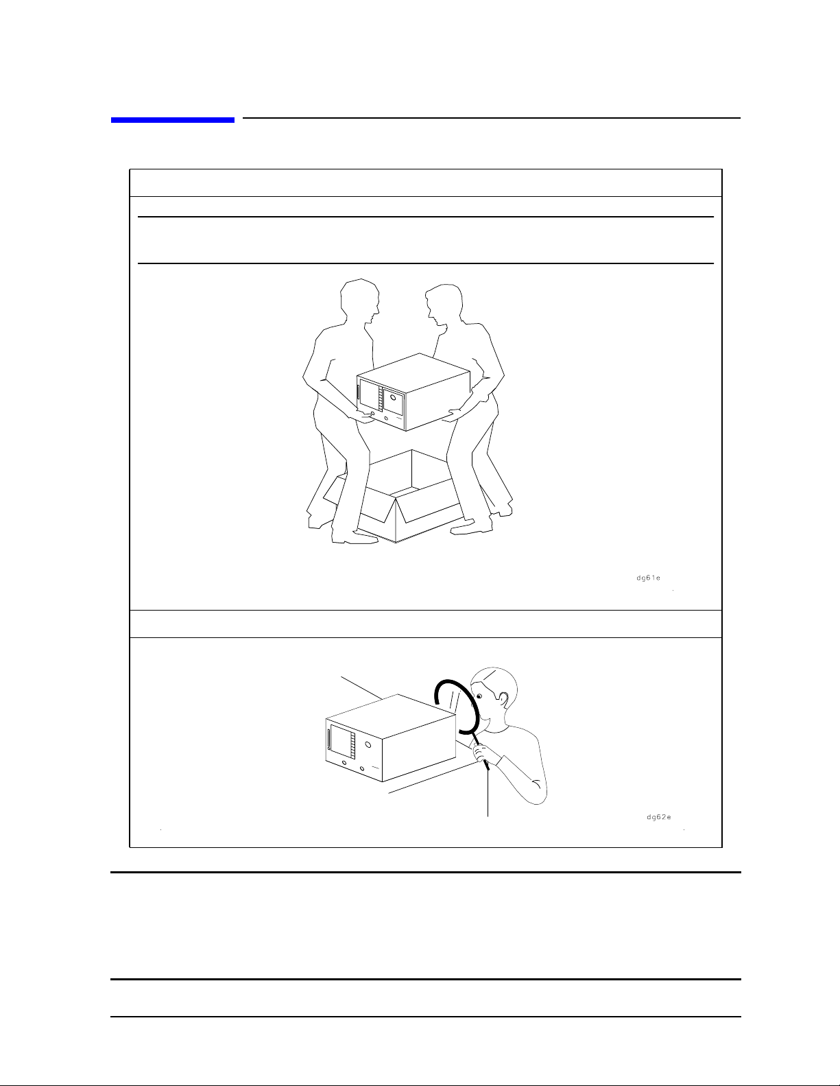
1. Unpack the contents of all the shipping containers.
WARNING The analyzer weighs approximately 46 pounds (21 kilograms). Use correct
lifting techniques.
2. Carefully inspect the analyzer to ensure that it was not damaged during shipment.
NOTE If your analyzer was damaged during shipment, contact your nearest Agilent
Technologies office or sales representative. A list of Agilent Technologies sales and
service offices is provided in Table 2-1 on page 2-28.
ES models only: the PORT 1 and PORT 2 connectors move. This is NOT a
defect.
Chapter 1 1-3
Page 10
Installing Your Analyzer
STEP 1. Verify the Shipment
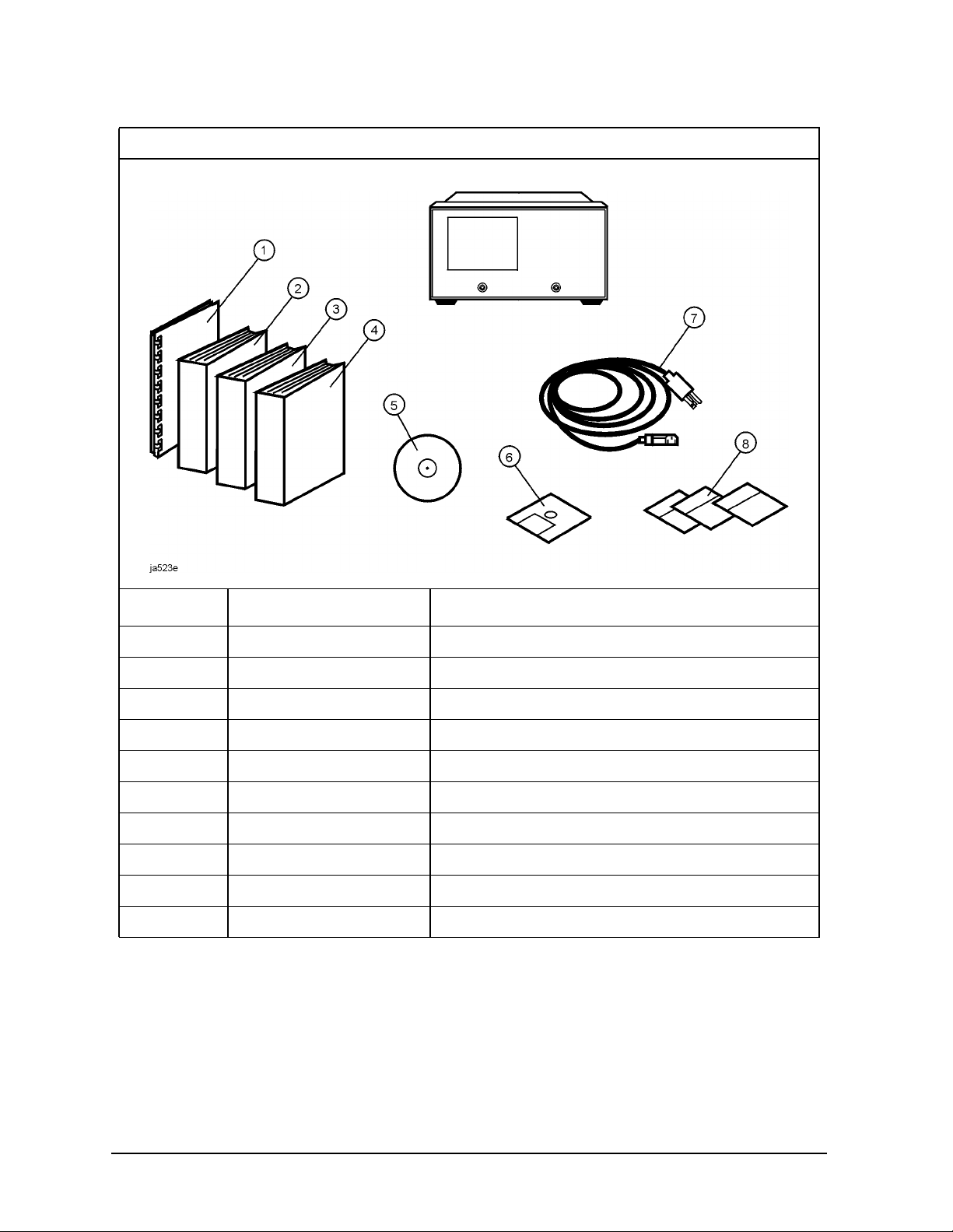
3. Verify that all the accessories have been included with the analyzer.
ItemNumber Part Number Description
1 08753-90471 Installation and Quick Start Guide
2 08753-90472 User's Guide
3 08753-90473 Reference Guide
4 08753-90475 Programmer’s Guide
5 08753-90469 CD-ROM
6 08753-10013 EEPROM Backup Disk
7 unique to country AC power cable
8 5062-9216 Rack Flange Kit (Option 1CM only)
8 5062-9236 Rack Flange Kit with Handles (Option 1CP only)
8 5062-9229 Front Handle Kit (standard)
1-4 Chapter1
Page 11
Installing Your Analyzer
STEP 2. Familiarize Yourself with the Analyzer Front and Rear Panels
STEP 2. Familiarize Yourself with the Analyzer Front and
Rear Panels
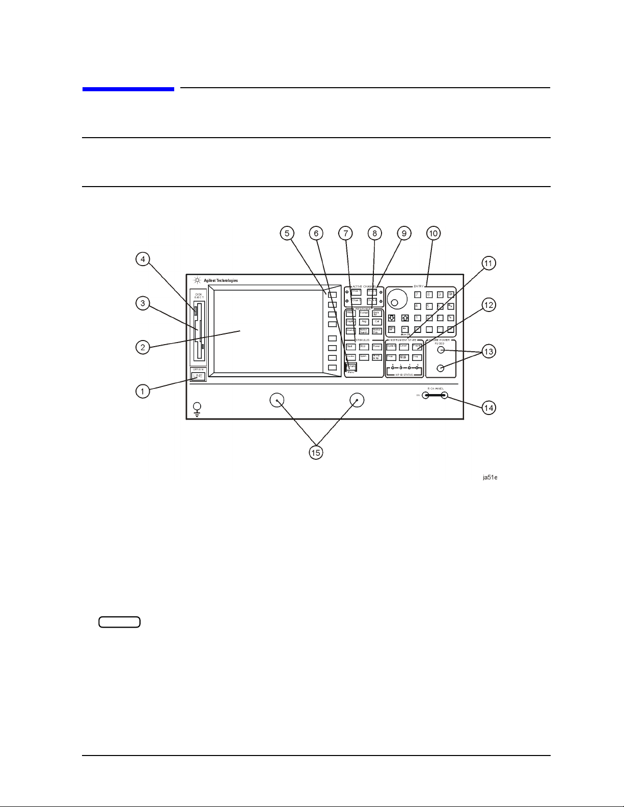
Analyzer Front Panel
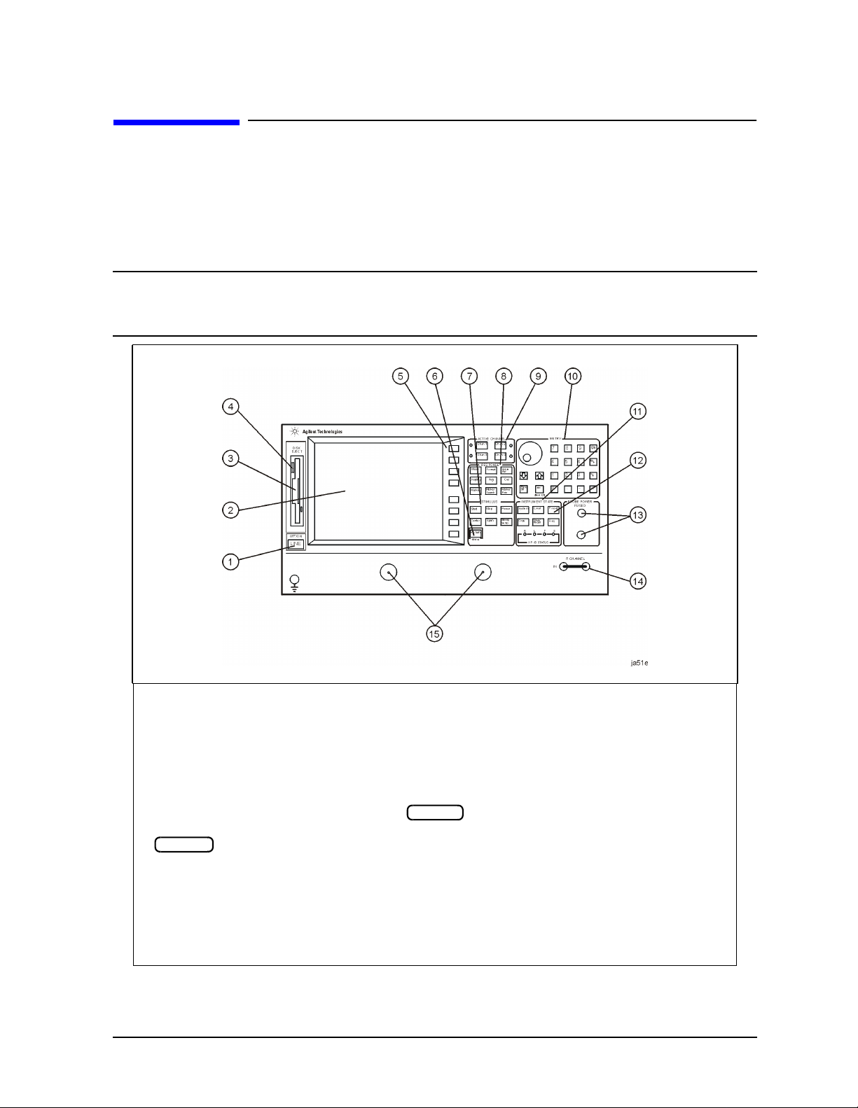
CAUTION Do not mistake the line switch for the disk eject button. See the figure below. If the
line switch is mistakenly pushed, the instrument will be turned off, losing all settings
and data that have not been saved.
1 LINE (power on/off) switch 8 RESPONSE function block
2 Display 9 ACTIVE CHANNEL keys
3 Disk drive 10 ENTRY block
4 Disk eject button 11 INSTRUMENT STATE function block
5 Softkeys
6 key
Return
7 STIMULUS function block 14 R CHANNEL connectors
Chapter 1 1-5
12 key
Preset
13 PROBE POWER connectors
15 ES models only:
PORT 1
and
PORT 2
ET models only:
REFLECTION
and
TRANSMISSION
Page 12
Installing Your Analyzer
STEP 2. Familiarize Yourself with the Analyzer Front and Rear Panels
Analyzer Rear Panel
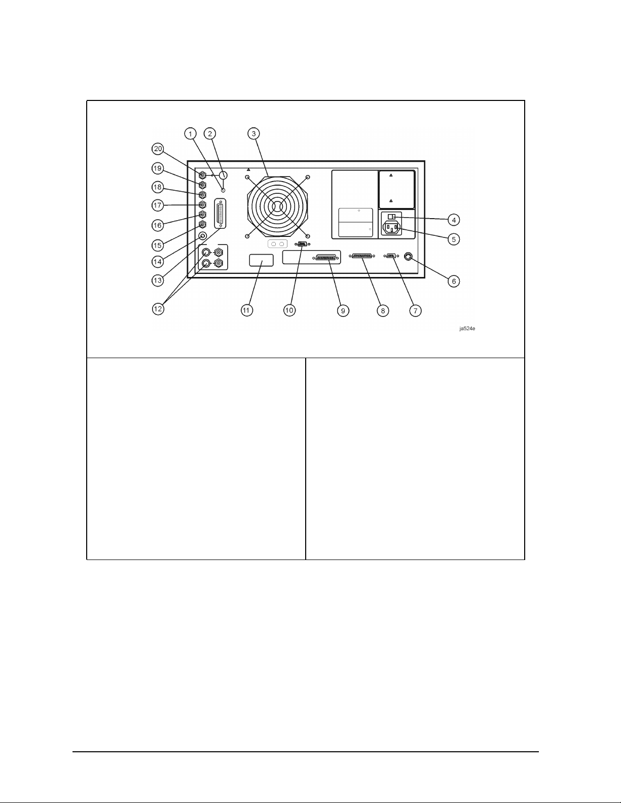
1 10 MHZ REFERENCE ADJUST
1
2 10MHZPRECISIONREFERENCE
OUTPUT
1
3 Fan
4 Line voltage selector switch
5 Power cord receptacle, with fuse
6 KEYBOARD input (mini-DIN)
7 RS-232 interface
8 PARALLEL interface
9 GPIB connector
10 EXTERNAL MONITOR: VGA
1.Option 1D5 only.
11 Serial number plate
12 BIAS INPUTS and FUSES
13 TEST SET I/O INTERCONNECT
14 MEASURE RESTART
15 LIMIT TEST
16 TEST SEQUENCE
17 EXTERNAL TRIGGER connector
18 EXTERNAL AM connector
19 AUXILIARY INPUT connector
20 EXTERNAL REFERENCE
INPUT connector
1-6 Chapter1
Page 13
Installing Your Analyzer
STEP 3. Meet Electrical and Environmental Requirements
STEP 3. Meet Electrical and Environmental Requirements
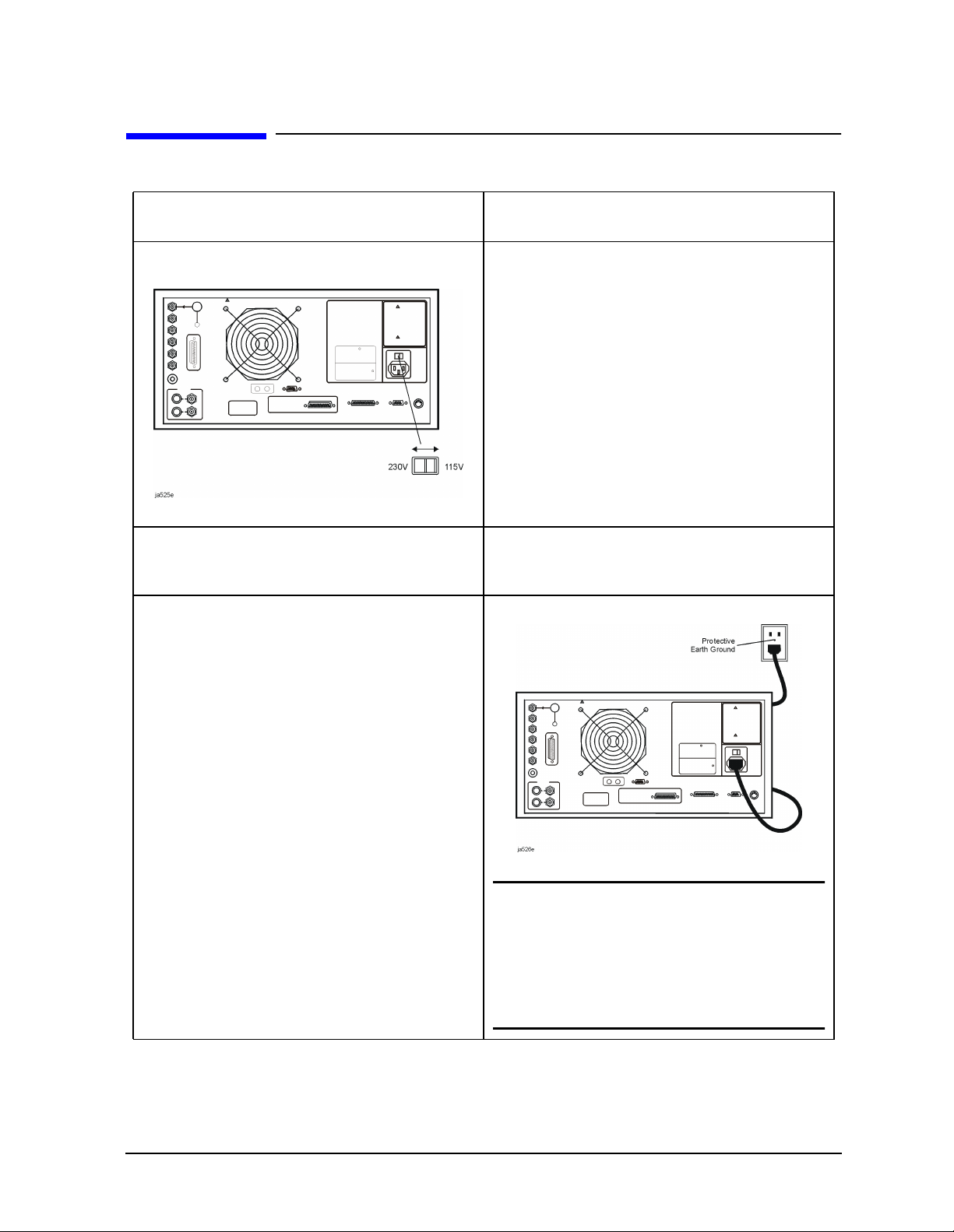
1. Set the line-voltage selector to the position
that corresponds to the AC power source.
3. Ensure the operating environment meets
the following requirements:
• 0 to 55 °C
2. Ensure the available AC power source
meets the following requirements:
• 90–132 VAC
• 47–66 Hz / 400 Hz (single phase)
- or -
• 198–265 VAC
• 47–66 Hz (single phase)
The analyzer power consumption is 350 VA
maximum.
4. Verify that the power cable is not damaged,
and that the power-source outlet provides a
protective earth contact.
• < 95% relative humidity at 40 °C
(non-condensing)
• < 15,000 feet (≈ 4,500 meters) altitude
Some analyzer performance parameters are
specified for 25 °C ±5 °C. Refer to the
Reference Guide for information on the
environmental compatibility of warranted
performance.
WARNING Any interruption of the
protective (grounding)
conductor or disconnection
of the protective earth
terminal, can result in
personal injury, or may
damage the analyzer.
Chapter 1 1-7
Page 14
Installing Your Analyzer
STEP 3. Meet Electrical and Environmental Requirements
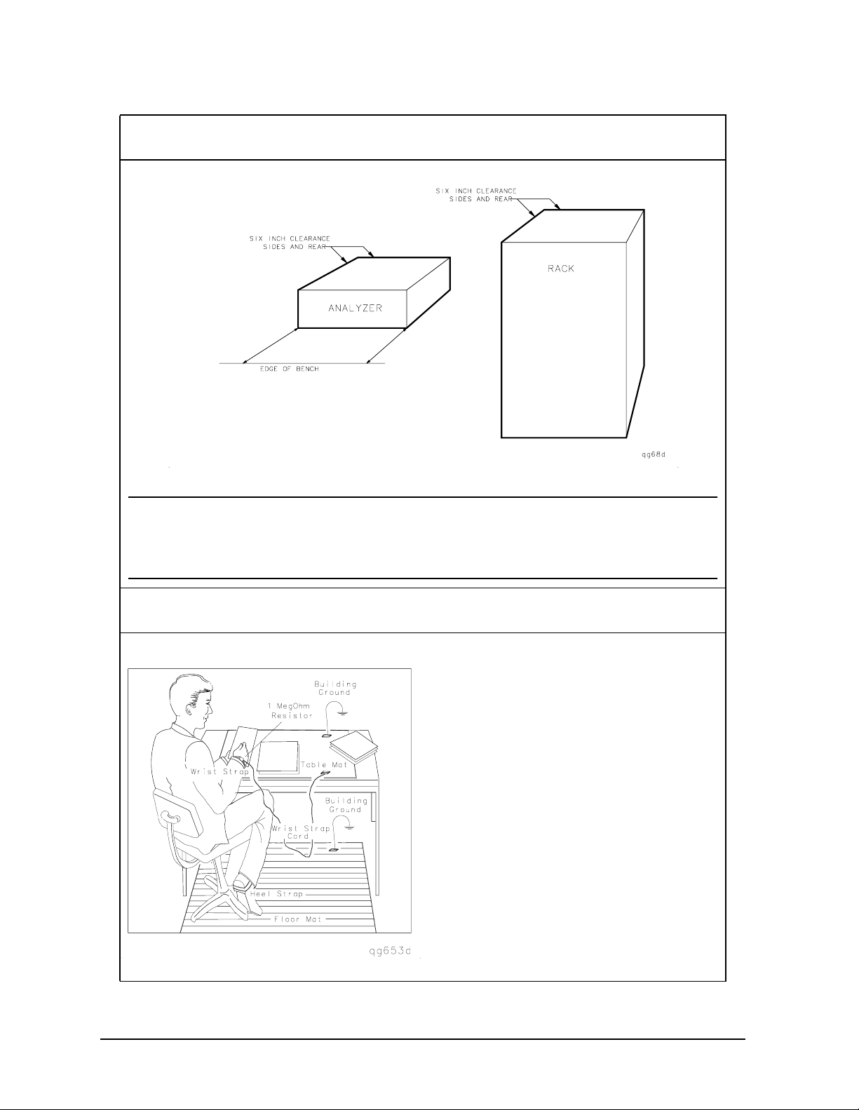
5. Ensure there are at least six inches of clearance between the sides and back of either the
stand-alone analyzer or the system cabinet.
CAUTION The environmental temperature must be 4 °C less than the maximum
operating temperature of the analyzer for every 100 watts dissipated in the
cabinet. If the total power dissipated in the cabinet is >800 watts, then you
must provide forced convection.
6. Set up a static-safe workstation. Electrostatic discharge (ESD) can damage or destroy
electronic components.
• static-control table mat and earth
ground wire: part number 9300-0797
• wrist-strap cord: part number 9300-0980
• wrist-strap: part number 9300-1367
• heel-straps: part number 9300-1308
• floor mat: not available through Agilent
Technologies
1-8 Chapter1
Page 15

STEP 4. Configure the Analyzer
STEP 4. Configure the Analyzer
This step shows you how to set up your particular analyzer configuration.
• standard configuration
• Option 1D5 configuration − high stability frequency reference
• printer or plotter configuration
• rack-mount configuration
Installing Your Analyzer
Chapter 1 1-9
Page 16
Installing Your Analyzer
STEP 4. Configure the Analyzer
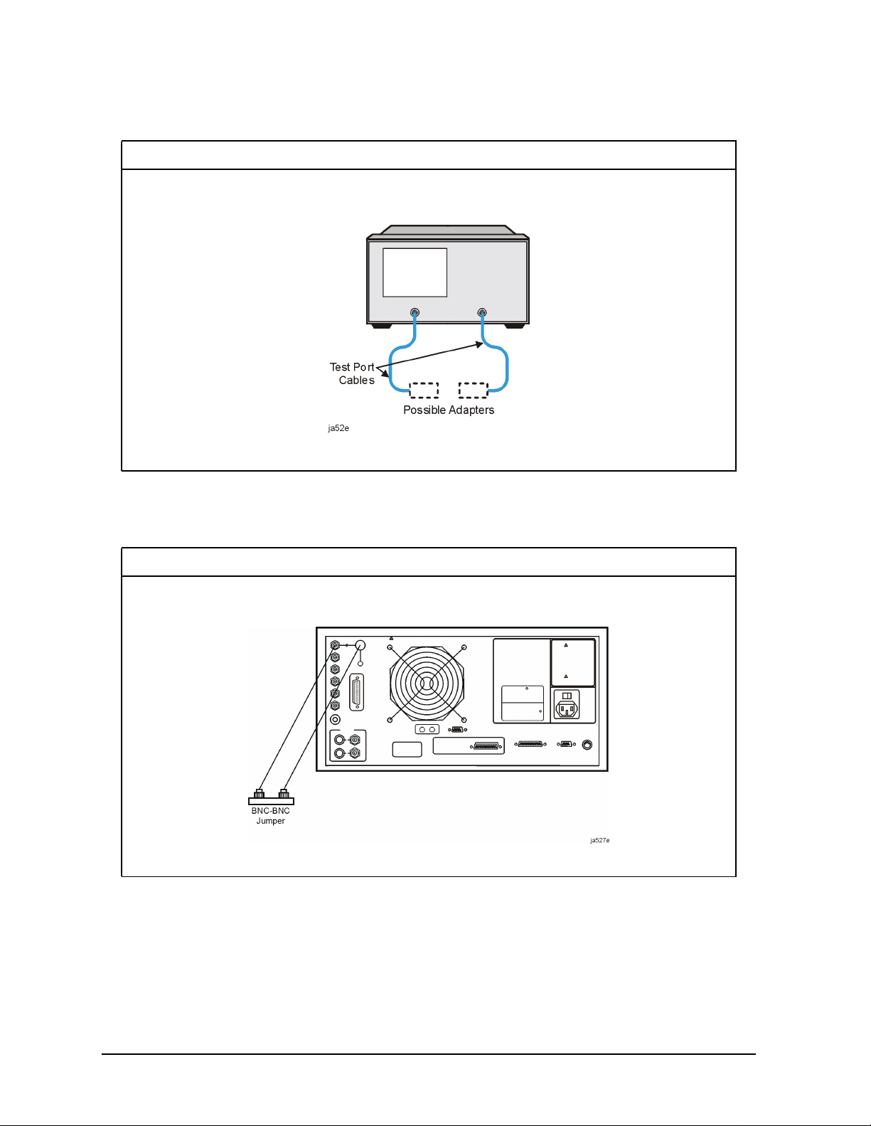
To Configure the Standard Analyzer
Connect test port cables and optional adapters if you are using other connector types.
To Configure an Analyzer with a High Stability Frequency
Reference (Option 1D5)
Connect the jumper cable on the analyzer rear panel as shown.
1-10 Chapter1
Page 17
STEP 4. Configure the Analyzer
PARALLEL
COPY
GPIO
COPY
GPIO
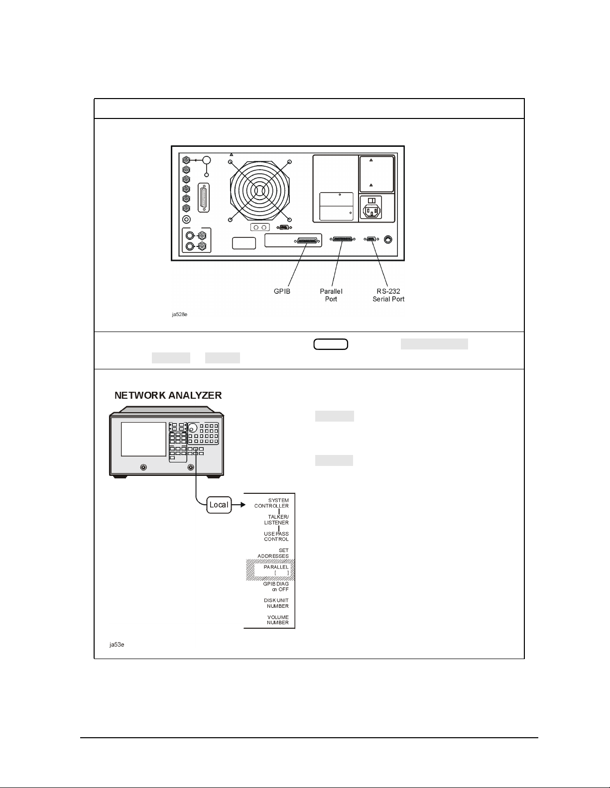
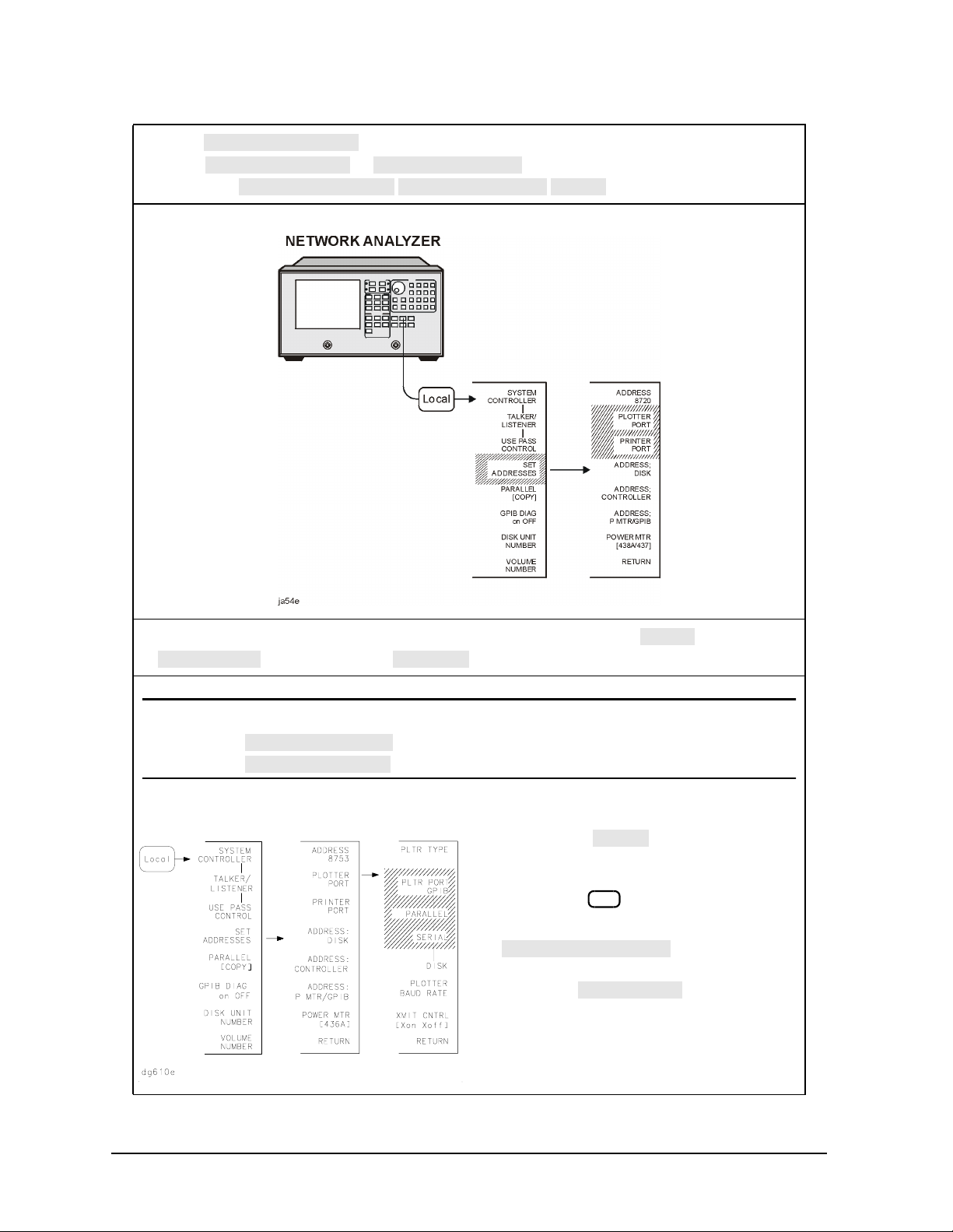
To Configure the Analyzer with Printers or Plotters
1. Connect your printer or plotter to the corresponding interface.
Installing Your Analyzer
2. If you are using the parallel interface, press and toggle until your
choice of or appears.
Local
If you choose:
the parallel port is dedicated for
normal copy device use (printers
or plotters).
the parallel port is dedicated for
general purpose I/O. The
analyzer controls the data input
oroutput through the sequencing
capability of the analyzer.
Chapter 1 1-11
Page 18
Installing Your Analyzer
SET ADDRESSES
PRINTER PORT
PLOTTER PORT
SET ADDRESSES
PLOTTER PORT
DISK
GPIB
PARALLEL
SERIAL
PLOTTER PORT
PRINTER PORT
GPIB
PARALLEL [COPY]
PARALLEL
STEP 4. Configure the Analyzer
3. Press . Then, depending on your printer/plotter device, choose
either or . Or, if you are plotting your files to
disk, press .
4. Press the key that corresponds to your printer or plotter interface: ,
(parallel port), or (serial port).
NOTE The plotter menu is shown as an example. It will only appear if you select
. Similar interface choices will appear if you select
.
• If you select , the GPIB address
selection is active. Enter the GPIB
address of your printer or plotter,
followed by .
• If you have already selected the
parallel-port configuration, you must
also select in this menu in
order to generate a printed or plotted
copy.
x1
choice for the
1-12 Chapter1
Page 19
Installing Your Analyzer
PLOTTER BAUD RATE
PRINTER BAUD RATE
PLOTTER PORT
XMIT CNTRL
Xon/Xoff
DTR/DSR
PRINTER PORT
Xon/Xoff
DTR/DSR
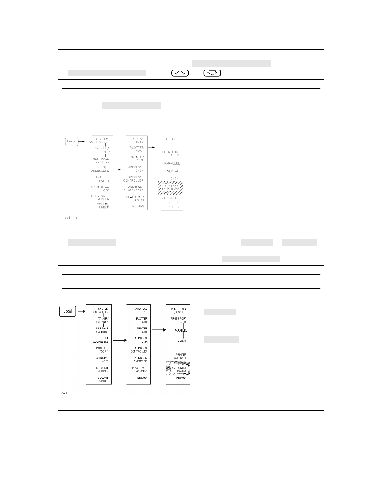
STEP 4. Configure the Analyzer
5. If you will be using the serial port, adjust the analyzer's baud rate until it is equal to the
baud rate set on the peripheral by pressing or
and the and front panel keys.
NOTE The plotter menu is shown as an example. It will only appear if you select
.
You can set the analyzer to the following
baud rates:
• 1200
• 2400
• 4800
• 9600
• 19200
6. Also, if you will be using the serial port, you must toggle the transmission control
(handshaking protocol) until your choice of or
appears (equal to the transmission control set on the peripheral). The printer menu is
shown as an example. It will only appear if you select .
NOTE Transmission control for plotters is set programmatically.
• sets transmission
on/transmission off (software
handshake).
• sets data terminal
ready/data set ready (hardware
handshake).
Chapter 1 1-13
Page 20

Installing Your Analyzer
STEP 4. Configure the Analyzer
7. If you will be creating a plot of the data, toggle until your choice of
PLOTTER
8. If you will be using a printer, toggle until your printer choice1 appears.
or appears.
HPGL PRT
PRNTR TYPE
PLTR TYPE
•Choose for a pen plotter.
•Choose for a PCL5
compatible printer.
PLOTTER
HPGL PRT
1
•Choose your printer type from these HP
printers:
THINKJET
❏
DESKJET
❏
(except for HP DeskJet 540 and
Deskjet 850C)
LASERJET
❏
PAINTJET
❏
DJ 540
❏ (for use with
HP DeskJet 540 and
Deskjet 850C—converts 100 dpi
raster information to 300 dpi raster
format)
•Choose for
EPSON-P2
Epson-compatible printers (ESC/P2
printer control language).
1.For a current printer compatibility guide, consult the web page at
http://www.agilent.com/find/pcg.
1-14 Chapter1
Page 21
Installing Your Analyzer
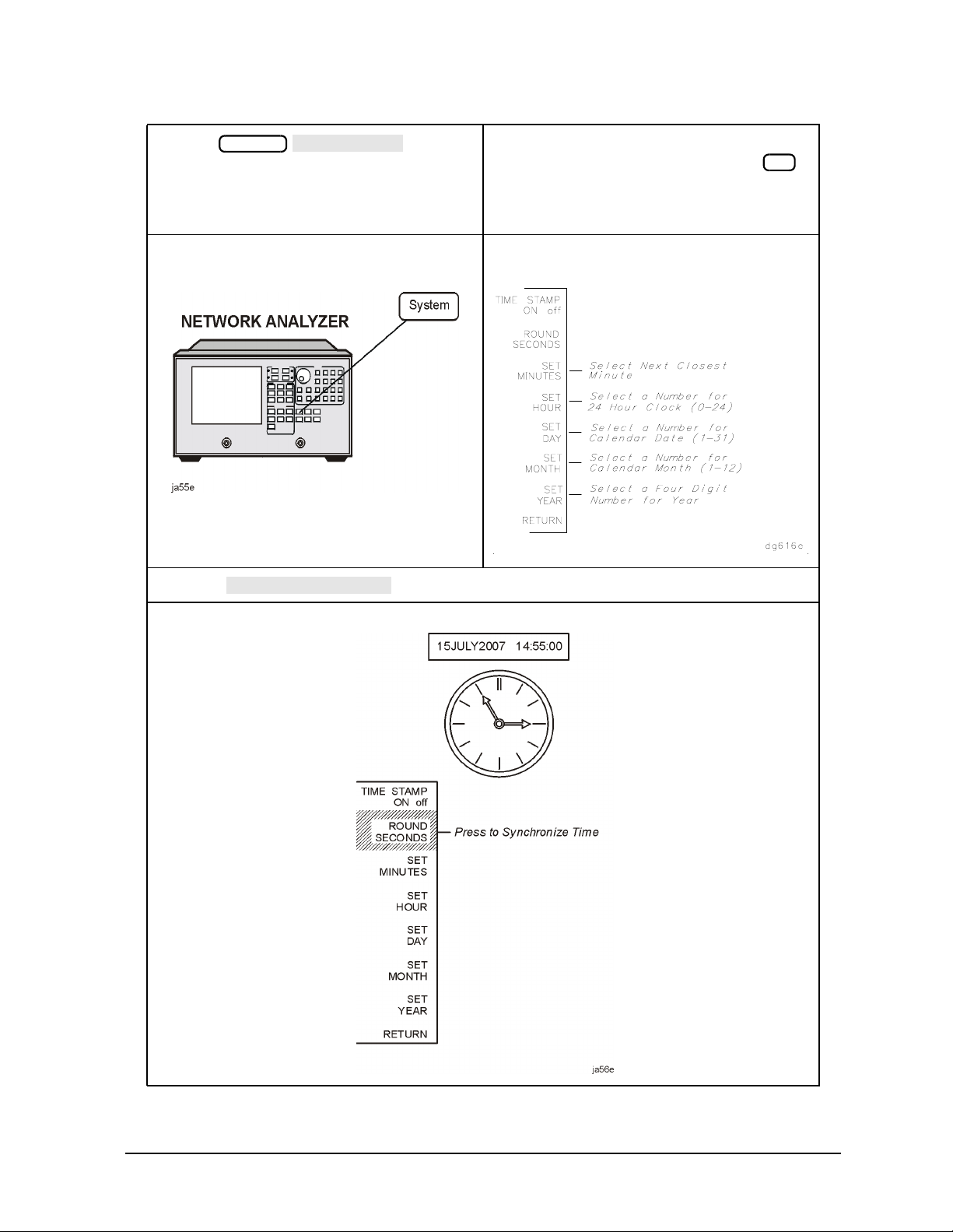
SET CLOCK
ROUND SECONDS
STEP 4. Configure the Analyzer
9. Press to begin
setting and activating the time stamp
feature so the analyzer places the time
and date on your hardcopies and disk
directories.
11. Press when the time is exactly as you have set it.
System
10. Press each of the following softkeys to
set the date and time, followed by .
x1
Chapter 1 1-15
Page 22

Installing Your Analyzer
STEP 4. Configure the Analyzer
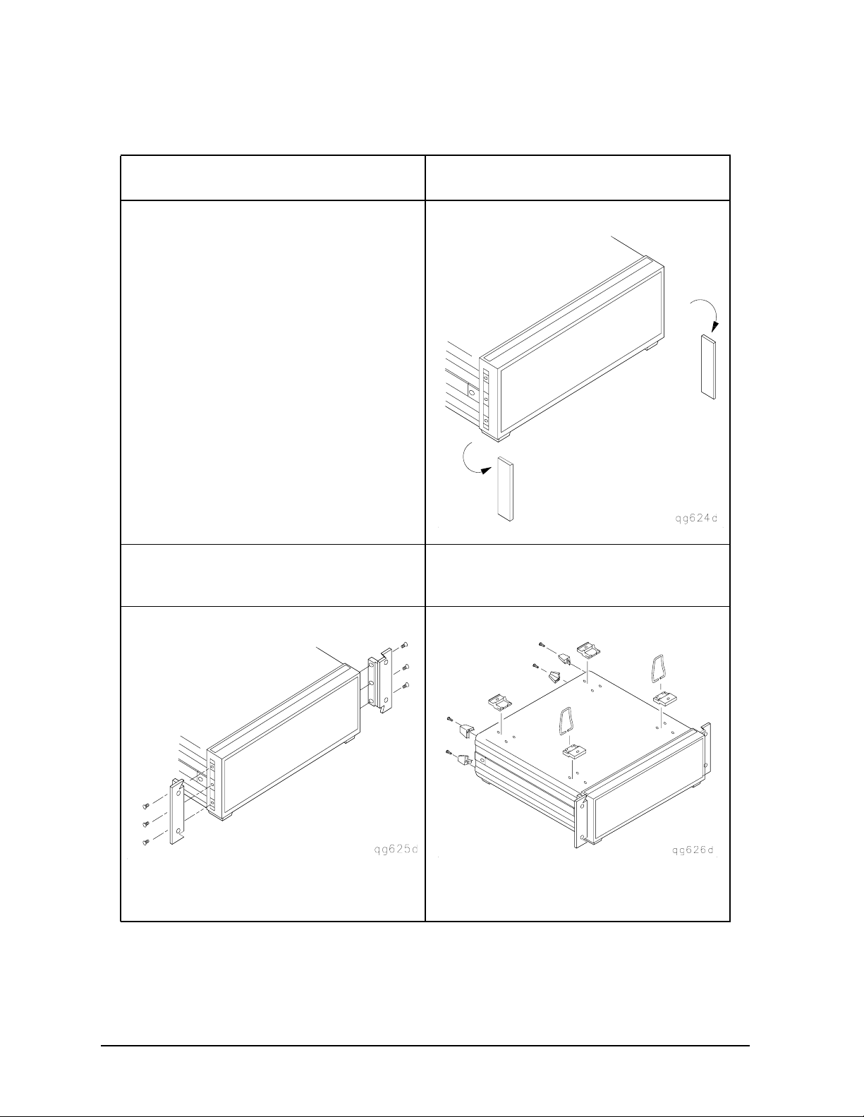
To Configure the Analyzer for Bench Top or Rack Mount Use
There are three kits available for the analyzer:
• instrument front handles kit (standard: part number 5062-9229)
• cabinet flange kit without front handles (Option 1CM: part number 5062-9216)
• cabinet flange kit with front handles (Option 1CP: part number 5062-9236)
1-16 Chapter1
Page 23
STEP 4. Configure the Analyzer
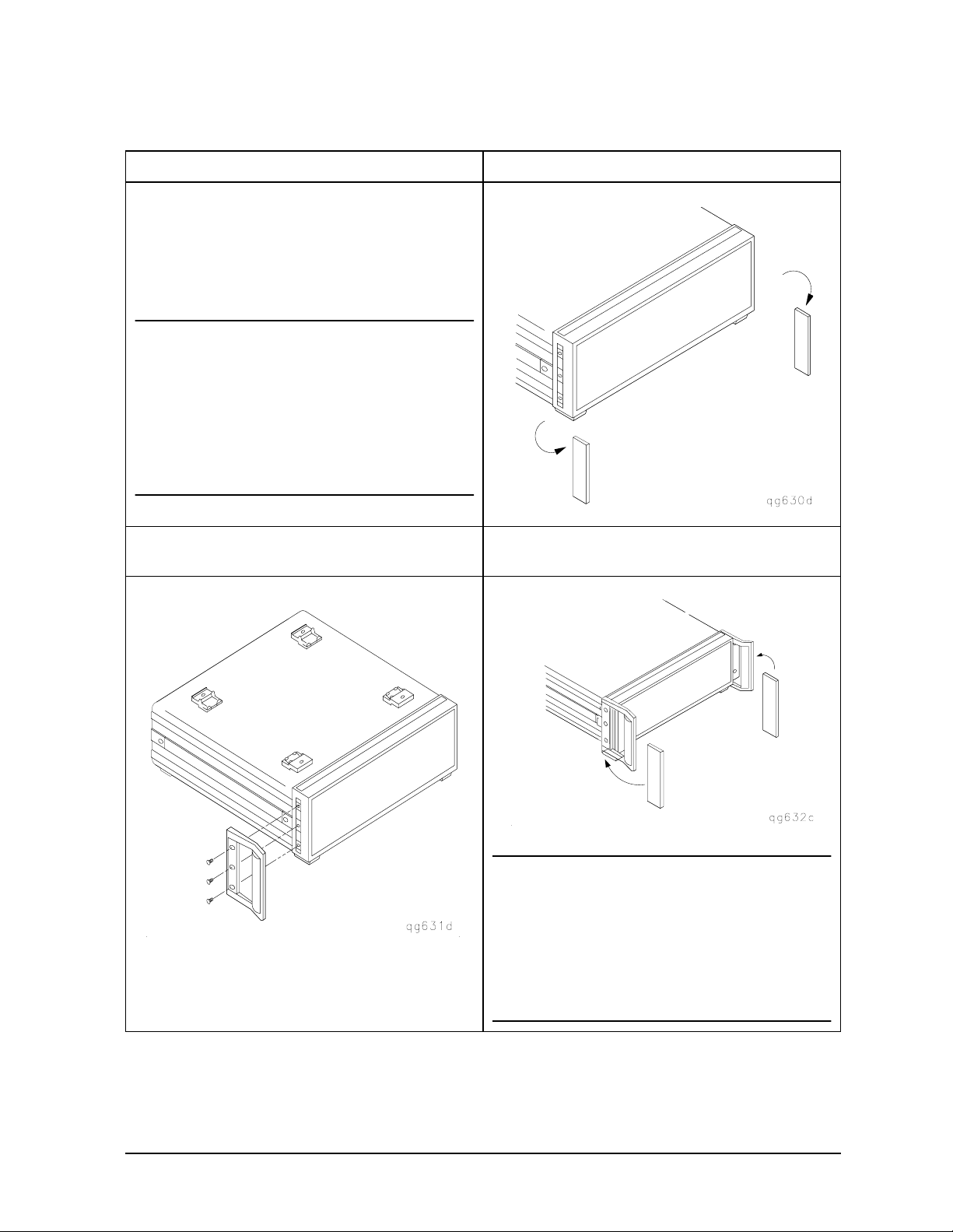
To Attach Front Handles to the Analyzer (Standard)
1. Ensure that the front handle kit is complete. 2. Remove the side trim strips.
• (2) front handles
• (6) screws
• (2) trim strips
NOTE If any items are damaged or
missing from the kit, contact the
nearest Agilent Technologies
sales or service office to order a
replacement kit.
Items within the kit (handles,
flanges, screws, etc.) are not
individually available.
Installing Your Analyzer
3. Attach the handles to the sides of the front
panel, using three screws for each handle.
4. Place the new trim strip over the screws on
the handles.
WARNING If an instrument handle is
damaged, you should replace
it immediately. Damaged
handles can break while you
are moving or lifting the
instrument and cause
personal injury or damage to
the instrument.
Chapter 1 1-17
Page 24
Installing Your Analyzer
STEP 4. Configure the Analyzer
To Attach Cabinet Flanges without Front Handles to the Analyzer
(Option 1CM)
1. Ensure that the cabinet flange kit is
complete.
• (2) cabinet mount flanges
• (6) screws
3. Attach the cabinet flanges to the sides of
the front panel using three screws for
each flange.
2. Remove side trim strips.
4. Remove the feet and the tilt stands before
cabinet mounting the instrument.
1-18 Chapter1
Page 25

STEP 4. Configure the Analyzer
To Attach Cabinet Flanges with Front Handles to the Analyzer
(Option 1CP)
Installing Your Analyzer
1. Ensure that the cabinet flange kit with
handles is complete.
• (2) cabinet mount flanges
• (2) front handles
• (6) screws
3. Attach the cabinet mount flanges and the
handles to the sides of the front panel, using
three screws per side. (Attach the flanges to
the outside of the handles.)
2. Remove the side trim strips.
4. Remove the feet and the tilt stands before
cabinet mounting the instrument.
WARNING If an instrument handle is
damaged, you should
replace it immediately.
Damaged handles can break
while you are moving or
lifting the instrument and
cause personal injury or
damage to the instrument.
Chapter 1 1-19
Page 26

Installing Your Analyzer
STEP 5. Verify the Analyzer Operation
STEP 5. Verify the Analyzer Operation
The following procedures show you how to check your analyzer for correct operation:
• viewing installed options
• initiating self-test
• running operator's check
• testing transmission mode
• testing reflection mode
NOTE If the analyzer should fail any of the following tests, call the nearest Agilent
Technologies sales or service office to determine the type of warranty you
have. If repair is necessary, send the analyzer (and the EEPROM backup
disk) to the nearest Agilent Technologies service center with a description of
any failed test and any error message. Ship the analyzer using the original
packaging materials. Returning the analyzer in anything other than the
original packaging may result in non-warranted damage. A table listing of
Agilent Technologies sales and service offices is provided in Table 2-1 on
page 2-28.
NOTE The illustrations depicting the analyzer display were made using an ES
model. Other analyzer displays may appear different, depending on model
and options.
1-20 Chapter1
Page 27

To View the Installed Options
SERVICE MENU
FIRMWARE REVISION
Installing Your Analyzer
STEP 5. Verify the Analyzer Operation
1. Cycle the AC power using the LINE switch, or press
.
2. Locate the serial number and configuration options. Compare them to the shipment
documents.
System
Chapter 1 1-21
Page 28

Installing Your Analyzer
STEP 5. Verify the Analyzer Operation
To Initiate the Analyzer Self-Test
1. Cycle the AC power using the LINE switch.
2. Watch for the following indications that the analyzer is operating correctly:
1-22 Chapter1
Page 29

To Run the Operator's Check
SERVICE MENU
TESTS
EXTERNAL TESTS
EXECUTE TEST
CONTINUE
EXECUTE TEST
CONTINUE
EXECUTE TEST
CONTINUE
Installing Your Analyzer
STEP 5. Verify the Analyzer Operation
1. Connect the equipment as shown.
3. ET models only: Press
. Follow the prompts
shown on the analyzer display and then
press .
2. Press
Follow the prompts shown on the analyzer
display and then press .
3. ES models only: Press
shown on the analyzer display and then
press .
Preset System
. Follow the prompts
.
Chapter 1 1-23
Page 30

Installing Your Analyzer
Trans: FWD S21(B/R)
TRANSMISSN
Trans: REV S12 (A/R)
STEP 5. Verify the Analyzer Operation
To Test the Transmission Mode
1. Connect the equipment as shown and press.2. Check the forward transmission mode for
Preset Chan 2 Meas
channel 2 by pressing
or .
NOTE The test port return cable
should have low-loss
characteristics to avoid a
degradation in frequency
response at higher frequencies.
3. Look at the measurement trace displayed
on the analyzer. It should be similar to the
trace below.
4. ES models only: To check the reverse
transmission mode for channel 2, press
Meas
measurement trace should be similar to the
trace below.
. The
1-24 Chapter1
Page 31

Installing Your Analyzer
Refl: REV S22 (B/R)
STEP 5. Verify the Analyzer Operation
To Test the Reflection Mode
1. Connect the equipment as shown and press.2. Look at the measurement trace displayed
Preset
on the analyzer. It should be similar to the
trace below.
3. ES models only: Check the reverse
reflection mode for channel 1 by pressing
Meas
measurement trace should be similar to the
trace shown below.
. The
4. If you are ready to start making
measurements, continue with the next
chapter, “Quick Start: Learning How to
Make Measurements.”
Chapter 1 1-25
Page 32

Installing Your Analyzer
FILE UTILITIES
FORMAT DISK
FORMAT:LIF
FORMAT:DOS
FORMAT INT DISK
YES
SERVICE MENU
SERVICE MODES
MORE
STORE EEPR
SELECT DISK
INTERNAL DISK
RETURN
SAVE STATE
STEP 6. Back Up the EEPROM Disk
STEP 6. Back Up the EEPROM Disk
Description
Correction constants are stored in EEPROM on the A9 controller assembly. The advantage
of having an EEPROM backup disk is the ability to store all the correction-constant data to
a new or repaired A9 assembly without having to rerun the correction-constant
procedures. The analyzer is shipped from the factory with an EEPROM backup disk which
is unique to each instrument. It is prudent to make a copy of the EEPROM backup disk so
that it can be used in case of failure or damage to the original backup disk.
Equipment
3.5-inch disk.......................................................................................92192A (box of 10)
CAUTION Do not mistake the line switch for the disk eject button. If the line switch is
mistakenly pushed, the instrument will be turned off, losing all settings and
data that have not been saved.
EEPROM Backup Disk Procedure
1. Press .
2. Insert a 3.5-inch disk into the analyzer disk drive.
3. If the disk is not formatted, press .
• To format a LIF disk, select (The supplied EEPROM backup disk is
• To format a DOS disk, select .
Press and answer at the query.
4. Press . Toggle
to ON. Then press
NOTE A default file “FILE00” is created. The file name appears in the upper
Preset
Save/Recall
LIF. The analyzer does not support LIF-HFS format.)
System
Save/Recall
to store the correction-constants data onto floppy disk.
left-hand corner of the display. The file type “ISTATE(E)” describes the file as
an instrument-state with EEPROM backup.
1-26 Chapter1
Page 33

Installing Your Analyzer
FILE UTILITIES
RENAME FILE
ERASE TITLE
SELECT LETTER
DONE
STEP 6. Back Up the EEPROM Disk
5. Press . Use the front panel knob
and the softkey to rename the file “FILE00” to “N12345” where
12345 represents the last 5 digits of the instrument's serial number. (The first character
in the file name must be a letter.) When finished, press .
6. Label the disk with the serial number of the instrument, the date, and the words
“EEPROM Backup Disk.”
NOTE Whenever the analyzer is returned to Agilent Technologies for servicing
and/or calibration, the EEPROM backup disk should be returned with the
analyzer. This will significantly reduce the instrument repair time.
7. The EEPROM backup disk procedure is now complete.
Chapter 1 1-27
Page 34

2 Quick Start: Learning How to Make
Measurements
2-1
Page 35

Quick Start: Learning How to Make Measurements
Introduction
Introduction
The information and procedures in this chapter teach you how to make measurements and
what to do if you encounter a problem with your analyzer. The following sections are
included:
• Front Panel
• Measurement Procedure
• Learning to Make Transmission Measurements
• Learning to Make Reflection Measurements
• If You Encounter a Problem
NOTE The illustrations depicting the analyzer display were made using an ES
model. Other analyzer displays may appear different, depending on model
and options.
2-2 Chapter2
Page 36
Quick Start: Learning How to Make Measurements
Analyzer Front Panel
Analyzer Front Panel
CAUTION Do not mistake the line switch for the disk eject button. See the figure below.
If the line switch is mistakenly pushed, the instrument will be turned off,
losing all settings and data that have not been saved.
Figure 2-1 The Analyzer Front Panel
1. LINE switch. This switch controls AC power to the analyzer. 1 is on, 0 is off.
2. Display. This shows the measurement data traces, measurement annotation, and
softkey labels.
3. Disk drive. This 3.5-inch drive allows you to store and recall instrument states and
measurement results for later analysis.
4. Disk eject button. This button ejects the disk from the disk drive.
5. Softkeys. These keys provide access to menus that are shown on the display.
6. key. This key returns the previous softkey menu shown on the display.
Return
7. STIMULUS function block. The keys in this block allow you to control the analyzer
source's frequency, power, and other stimulus functions.
8. RESPONSE function block. The keys in this block allow you to control the
measurement and display functions of the active display channel.
Chapter 2 2-3
Page 37

Quick Start: Learning How to Make Measurements
Analyzer Front Panel
9. ACTIVE CHANNEL keys. The analyzer has four independent display channels.
These keys allow you to select the active channel. Then any function you enter applies
to this active channel. Notice that the light next to the current active channel’s key is
illuminated.
10. The ENTRY block. This block includes the knob, the step keys, and the
number pad. These allow you to enter numerical data and control the markers.
You can use the numeric keypad to select digits, decimal points, and a minus sign for
numerical entries. You must also select a units terminator to complete value inputs.
11. INSTRUMENT STATE function block. These keys allow you to control
channel-independent system functions such as the following:
• copying, save/recall, and GPIB controller mode
• limit testing
• tuned receiver mode
• frequency offset mode (Option 089)
• test sequence function
• harmonic measurements (Option 002)
• time domain transform (Option 010)
GPIB STATUS indicators are also included in this block.
12. key. This key returns the instrument to either a known factory preset state, or
Preset
a user preset state that can be defined. Refer to the “Preset State and Memory
Allocation” chapter in the Reference Guide for a complete listing of the instrument
preset condition.
13. PROBE POWER connectors. These connectors (fused inside the instrument) supply
power to an active probe for in-circuit measurements of AC circuits.
14. R CHANNEL connectors. (ES models only) These connectors allow you to apply an
input signal to the analyzer's R channel, for frequency offset mode.
15. ES models only: PORT 1 and PORT 2. These ports output a signal from the source
and receive input signals from a device under test. PORT 1 allows you to measure S
12
and S11. PORT 2 allows you to measure S21 and S22.
ET models only: REFLECTION and TRANSMISSION. The REFLECTION port
allows you to make reflection measurements, outputting a signal from the source and
receiving input signals from a device under test. The TRANSMISSION port allows you
to make transmission measurements, receiving input signals from a device under test.
2-4 Chapter2
Page 38

Quick Start: Learning How to Make Measurements
Measurement Procedure
Measurement Procedure
This is a general measurement procedure that is used throughout the guide to illustrate
the use of the analyzer.
Step 1. Choose measurement parameters with your test device
connected
• Press the key to return the analyzer to a known state.
• Connect your device under test (DUT) to the analyzer.
CAUTION Damage may result to the DUT if it is sensitive to the analyzer's default
• Choose the settings that are appropriate for the intended measurement.
❏ measurement type (S
❏ frequencies
❏ number of points
❏ power
❏ measurement trace format
• Make adjustments to the parameters while you are viewing the device response.
Preset
output power level. To avoid damaging a sensitive DUT, be sure to set the
analyzer's output power to an appropriate level before connecting the DUT to
the analyzer.
or reflection, for example)
11
Step 2. Make a measurement calibration
Press the key to begin to perform a measurement calibration using a known set of
standards (a calibration kit). Error-correction establishes a magnitude and phase
reference for the test setup and reduces systematic measurement errors.
Cal
Step 3. Measure the device
• Reconnect the device under test.
• Use the markers to identify various device response values if desired.
Step 4. Output measurement results
• Store the measurement file to a disk.
• Generate a hardcopy with a printer or plotter.
Chapter 2 2-5
Page 39
Quick Start: Learning How to Make Measurements
Trans: FWD S21 (B/R)
TRANSMISSN
AUTO SCALE
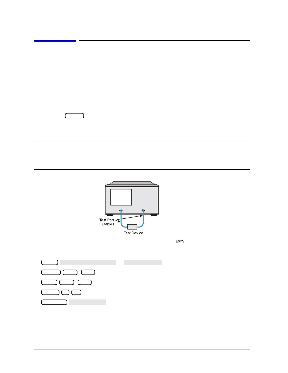
Learning to Make Transmission Measurements
Learning to Make Transmission Measurements
This example procedure shows you how to measure the transmission response of a
175 MHz bandpass filter. The measurement parameters listed are unique to this
particular test device.
For further measurement examples, refer to the “Making Measurements” chapter in the
User's Guide.
Step 1. Choose the measurement parameters with your test device connected
1. Press the key to return the analyzer to a known state.
Preset
2. Connect your test device to the analyzer as shown in Figure 2-2. Use adapters where
appropriate.
CAUTION Damage may result to the device under test if it is sensitive to the analyzer's
default output power level. Toavoid damaging a sensitive DUT, be sure to set
the analyzer's output power to an appropriate level before connecting the
DUT to the analyzer.
Figure 2-2 Device Connections for a Transmission Measurement
3. Choose the following measurement settings:
Meas
Center 200 M/µ
Span 375 M/µ
Power 5 x1
Scale Ref
4. Look at the device response to determine if these are the parameters that you want for
your device measurement. For example, if the trace is noisy you may want to increase
the test port output power (which increases the analyzer input power), reduce the IF
bandwidth, or add averaging. Or, to better see an area of interest, you may want to
change the test frequencies.
2-6 Chapter2
or
Page 40
Quick Start: Learning How to Make Measurements
CALIBRATE MENU
RESPONSE
THRU
SELECT DISK
INTERNAL MEMORY
INTERNAL DISK
EXTERNAL DISK
RETURN
SAVE STATE
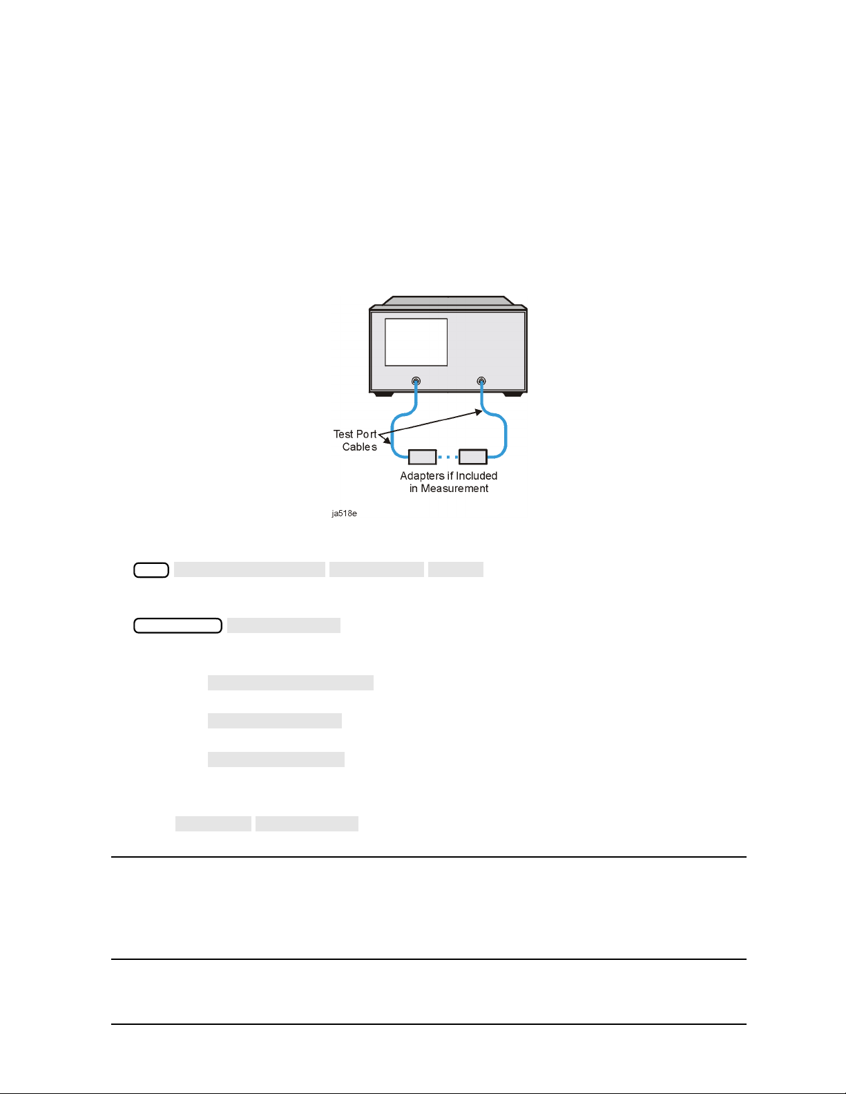
Learning to Make Transmission Measurements
Step 2. Perform a measurement calibration
1. Disconnect your test device from the analyzer.
2. Connect a “thru” between the measurement cables, as shown in Figure 2-3. Include all
the adapters that you will use in your device measurement.
If noise reduction techniques are needed for the measurement, the instrument's
settings (reduced IF BW, and /or averaging) should be selected prior to any
error-correction.
Figure 2-3 Connections for a “Thru” Calibration Standard
3. Press the following keys to make a transmission response calibration:
Cal
4. To save the error-correction (measurement calibration), press:
Save/Recall
5. Next, choose from the following options:
• Choose if you want to save the calibration results and
instrument state to the analyzer's memory.
• Choose if you want to save the calibration results and
instrument state to the disk that is in the analyzer's internal disk drive.
• Choose if you want to save the calibration results and
instrument state to the disk that is in an (optional) external disk drive that is
configured to the analyzer.
6. Press to save the error-correction (measurement calibration).
NOTE Example procedures for all types of error-correction (measurement
calibrations) are located in the “Calibrating For Increased Measurement
Accuracy” chapter in the User's Guide. For information on the analyzer
operation during error-correction (measurement calibration), refer to the
“Operating Concepts” chapter in the User's Guide.
Chapter 2 2-7
Page 41

Quick Start: Learning How to Make Measurements
AUTO SCALE
Learning to Make Transmission Measurements
Step 3. Measure the device
Measuring Insertion Loss
1. Reconnect your test device as in Figure 2-2.
2. Reposition the measurement trace for the best view. This can be done by pressing
Scale Ref
position, or the scale/division.
and, if necessary, adjusting the reference level, reference
3. Press and turn the front panel knob to place the marker at a frequency of
Marker
interest. Read the device's insertion loss to 0.001 dB resolution as shown in Figure 2-4.
The analyzer shows the frequency of the marker location in the active entry area
(upper-left corner of display). The analyzer also shows the amplitude and frequency of
the marker location in the upper-right corner of the display.
Figure 2-4 Example Measurement of Insertion Loss
2-8 Chapter2
Page 42

Quick Start: Learning How to Make Measurements
SELECT DISK
INTERNAL DISK
RETURN
DEFINE DISK-SAVE
DATA ARRAY on OFF
RAW ARRAY on OFF
FORMAT ARY on OFF
GRAPHICS on OFF
DATA ONLY on OFF
DATA ONLY on OFF
DATA ONLY ON off
SAVE USING BINARY
SAVE USING ASCII
RETURN
SAVE STATE
Learning to Make Transmission Measurements
Step 4. Output measurement results
This example procedure shows how to output (store) measurement results to a disk.
For more information on creating a hardcopy of the measurement results, refer to
the "Printing, Plotting, and Saving Measurement Results" chapter in the User's Guide.
CAUTION Do not mistake the line switch for the disk eject button. If the line switch is
mistakenly pushed, the instrument will be turned off, losing all settings and
data that have not been saved.
1. Insert a DOS- or LIF-formatted disk into the analyzer disk drive. The analyzer does not
support LIF-HFS (hierarchy file system).
2. Press . Choose to save the
Save/Recall
measurement results to the analyzer's internal disk drive.
3. Press .
• Toggle to ON if you want to store the error-corrected data on
disk with the instrument state.
• Toggle to ON if you want to store the raw data (ratioed and
averaged, but no error-correction) on disk with the instrument state.
• Toggle to ON if you want to store the formatted data on disk
with the instrument state.
• Toggle to ON if you want to store user graphics on disk with
the instrument state.
• Toggle to ON if you want to only store the measurement data
of the device under test. The analyzer will not store the instrument state and
error-correction (measurement calibration). Therefore, the saved data cannot be
retrieved into the analyzer.
NOTE Toggling to ON will override all of the other save
options. Because this type of data is only intended for computer
manipulation, the file contents of a save cannot be
recalled and displayed on the analyzer.
• Choose if you want to store data in a binary format.
• Choose if you want to store data in an ASCII format, to later
4. Press and the analyzer saves the file with a default title.
Chapter 2 2-9
read on a computer.
Page 43

Quick Start: Learning How to Make Measurements
SEARCH: MAX
MKR ZERO
MKR ZERO∆ REF=
WIDTHS on OFF
Learning to Make Transmission Measurements
Measuring Other Transmission Characteristics
Using the analyzer marker functions, you can derive several important filter parameters
from the measurement trace that is shown on the analyzer display.
Measuring 3 dB Bandwidth.
The analyzer can calculate your test device bandwidth between two equal power levels. In
this example procedure, the analyzer calculates the −3 dB bandwidth relative to the center
frequency of the filter.
1. Press and turn the front panel knob to move the marker to the center
Marker
frequency position of the filter passband. An alternative method is to press
Marker Search
which should put you very close to the center of the
passband.
You can also position the marker by entering a frequency location: for example, press
175 M/µ
2. Press to zero the delta marker magnitude and frequency (this
Marker
.
sets the delta marker reference). The −3 dB points will be relative to this marker.
The softkey label changes to showing you that the delta
∆
reference point is the small ∆ symbol.
3. Press to enter the marker search mode.
Marker Search
4. Toggle to ON.
The analyzer calculates the −3 dB bandwidth, the center frequency and the Q (quality
factor) of the test device and lists the results in the upper-right corner of the display.
Markers 3 and 4 indicate the location of the −3 dB points, as shown in Figure 2-5.
Figure 2-5 Example Measurement of 3 dB Bandwidth
2-10 Chapter2
Page 44

Quick Start: Learning How to Make Measurements
WIDTH VALUE
MARKER all OFF
Learning to Make Transmission Measurements
5. Press and enter .
−6 x1
The analyzer now calculates the bandwidth between −6 dB power levels.
6. Press when you are finished with this measurement.
Marker
Chapter 2 2-11
Page 45

Quick Start: Learning How to Make Measurements
MARKER 1
MKR ZERO
SEARCH: MIN
IF BW [ ]
AVERAGING on OFF
Learning to Make Transmission Measurements
Measuring Out-of-Band Rejection.
1. Press . The marker appears where you placed it during the bandwidth
measurement.
2. Press .
Marker Search
The marker automatically searches for the minimum point on the trace. The frequency
and amplitude of this point, relative to the delta symbol in the center of the filter
passband, appear in the upper-right corner of the display. This value is the difference
between the maximum power in the passband and the power in the rejection band, that
is, one of the peaks in the rejection band.
Figure 2-6 Example Measurement of Out-of-Band Rejection
NOTE You can use the marker search mode to search the trace for the maximum
3. If your measurement needs some noise reduction, you can reduce the IF bandwidth or
add averaging.
• To reduce the IF bandwidth, press .
• To add averaging, press , then toggle to ON.
2-12 Chapter2
point or for any target value. The target value can be an absolute level (for
example, −3 dBm) or a level relative to the location of the small delta symbol
(for example: −3 dB from the center of the passband).
Avg
Avg
Page 46

Quick Start: Learning How to Make Measurements
RECALL STATE
MODE MENU
REF = 1
MARKER 2
MARKER MODE MENU
MKR STATS on OFF
Learning to Make Transmission Measurements
Measuring Passband Flatness or Ripple.
Passbandflatness (or ripple) is the variation in insertion loss over a specified portion of the
passband.
Continue with the following steps to measure passband flatness or ripple.
1. Press (if necessary, scroll to the desired file using
panel keys). Press to recall the error-corrected transmission
Save/Recall
the and front
measurement that has no markers engaged.
2. Press and turn the front panel knob to move marker 1 to the left edge of the
Marker
passband.
3. Press to change the marker 1 position to the delta
∆
∆
reference point.
4. Press and turn the front panel knob to move marker 2 to the right edge of
the passband.
5. Press . Toggle to ON.
Marker Fctn
The analyzer calculates the mean, standard deviation, and peak-to-peak variation
between the ∆ reference marker and the active marker, and lists the results in the
upper-right corner of the display. The passband ripple is automatically shown as the
peak-to-peak variation between the markers.
Figure 2-7 Example Measurement of Passband Flatness or Ripple
Chapter 2 2-13
Page 47

Quick Start: Learning How to Make Measurements
Learning to Make Reflection Measurements
Learning to Make Reflection Measurements
This example procedure shows you how to measure the reflection response of a 175 MHz
bandpass filter. The measurement parameter values listed are unique to this particular
test device.
For further measurement examples, refer to the "Making Measurements" chapter in the
User's Guide.
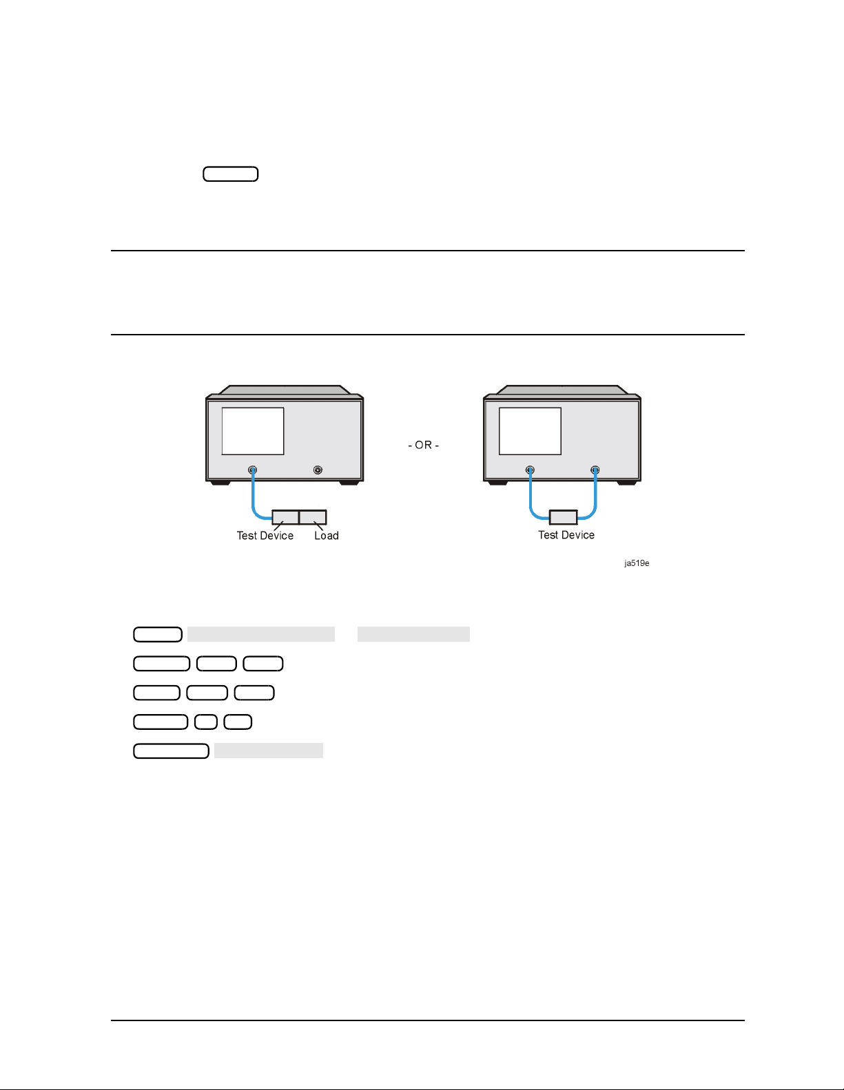
NOTE Reflection measurements monitor only one port of a test device. When a test
device has more than one port, you must ensure that the unused port(s) are
terminated in their characteristic impedance (for example, 50Ω or 75Ω). If
you do not terminate unused ports, reflections from these ports will cause
measurement errors. Figure 2-8 on page 2-15 illustrates two ways to
terminate an unused device port with the proper characteristic impedance.
The signal reflected from the device under test is measured as a ratio of the reflected
energy versus the incident energy. It can be expressed as reflection coefficient, return loss,
or standing-wave-ratio (SWR). These measurements are mathematically defined as
follows:
reflection coefficient (Γ) = reflected voltage / incident voltage
= S11 or S22 (magnitude and phase)
magnitude of reflection
coefficient (ρ)
return loss (dB) = −20 log (ρ), where ρ = |Γ|
standing-wave-ratio (SWR)
=|Γ|
= V
maximum
/ V
minimum
= (1 + ρ) / (1 −ρ)
2-14 Chapter2
Page 48
Quick Start: Learning How to Make Measurements
Refl: FWD S11 (A/R)
REFLECTION
AUTO SCALE
Learning to Make Reflection Measurements
Step 1. Choose measurement parameters with your test device
connected
1. Press the key to return the analyzer to a known state.
Preset
2. Connect your test device as shown in Figure 2-8. If using a load, make sure it has the
correct characteristic impedance.
CAUTION Damage may result to the device under test if it is sensitive to the analyzer's
default output power level. Toavoid damaging a sensitive DUT, be sure to set
the analyzer's output power to an appropriate level before connecting the
DUT to the analyzer.
Figure 2-8 Connections for Reflection Measurements
3. Choose the following measurement parameters:
Meas
Center 200 M/µ
Span 375 M/µ
Power 5 x1
Scale Ref
or
4. Look at the device response to determine if these are the measurement parameters that
you want. For example, if the trace is noisy you may want to increase the input power,
reduce the IF bandwidth, or add averaging. Tobetter see an area of interest, change the
test frequencies.
Chapter 2 2-15
Page 49
Quick Start: Learning How to Make Measurements
CAL KIT
SELECT CAL KIT
N 50
7mm
RETURN
CALIBRATE MENU
S11 1-PORT
REFLECTION 1-PORT
SHORT (M)
DONE 1-PORT CAL
DONE 1-PORT CAL
Learning to Make Reflection Measurements
Step 2. Make a measurement calibration
Follow these instructions to perform an S11 or reflection 1-port error correction:
1. Select a calibration kit that is appropriate to your device under test. Press
Cal
. Choose the calibration kit that is appropriate to your
test device by pressing the appropriate softkey. For example, if your test device uses
type-N 50Ω connectors, press . If your test device uses 7-mm connectors, press
Ω
, and so on.
2. Press twice, or
.
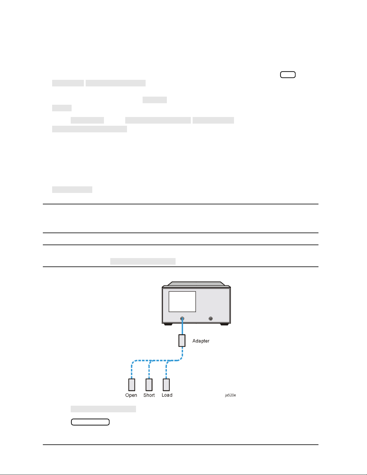
3. Follow the prompts shown on the analyzer display to connect and measure an open,
short, and load on PORT 1 or the REFLECTION port.
Any choice of male/female in the calibration process should always be made for the sex
that represents the test port. For example, if the test port had a male, type-N connector,
you would connect the female, type-N calibration device. But when you follow the
prompts on the analyzer to measure a short calibration standard, you would select
, or the sex that represents the test port.
NOTE To ensure an accurate error correction, you must connect the calibration
standards to the adapters or cables that you will include in the actual device
measurement.
NOTE If a mistake is made, standards can be measured more than once before
pressing . Only the last measurement data is used.
Figure 2-9 Connections for an S11 or Reflection 1-Port Error-Correction
4. Press after measuring the three standards.
5. Press .
Save/Recall
2-16 Chapter2
Page 50
Quick Start: Learning How to Make Measurements
SAVE STATE
AUTO SCALE
Learning to Make Reflection Measurements
6. Press to complete the process.
Step 3. Measure the device
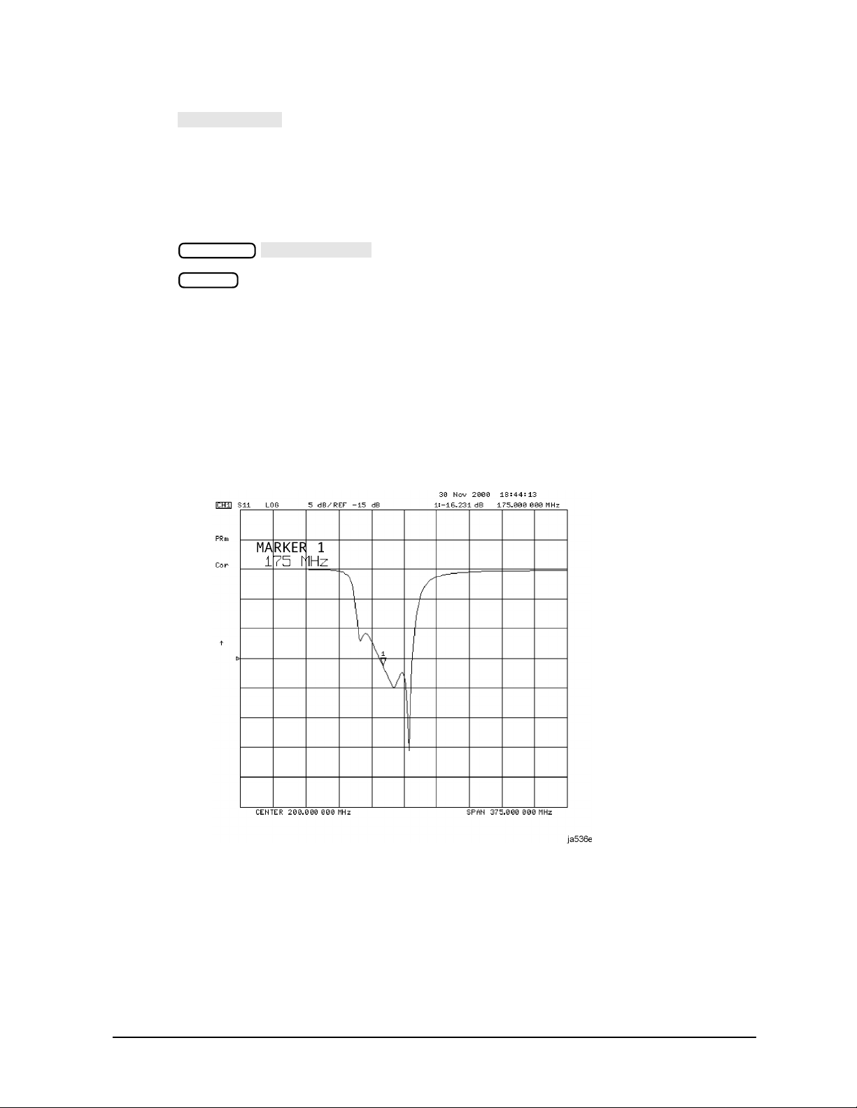
Measuring Return Loss.
1. Connect your device to PORT 1 or the REFLECTION port.
2. Press to reposition the trace.
3. Press to read the return loss from the analyzer display as shown in
Scale Ref
Marker
Figure 2-10.
The device response indicates that the filter and the analyzer impedances are better
matched within the frequency range of the filter passband than outside the passband.
That is, the reflected signal is smaller within the filter passband than outside the
passband.
In terms of return loss, the value within the passband is larger than outside the
passband. A large value for return loss corresponds to a small reflected signal just as a
large value for insertion loss corresponds to a small transmitted signal.
Figure 2-10 Example Measurement of Return Loss
Chapter 2 2-17
Page 51

Quick Start: Learning How to Make Measurements
MORE
TITLE
ERASE TITLE
DONE
SYSTEM CONTROLLER
PRINT MONOCHROME
Learning to Make Reflection Measurements
Step 4. Output measurement results
This step in the procedure shows you how to output the measurement results to a printer.
For in-depth information on creating a hardcopy of the measurement results, refer to the
“Printing, Plotting, and Saving Measurement Results” chapter in the User's Guide.
1. Connect a printer to the analyzer as described in “To Configure the Analyzer with
Printers or Plotters” on page 1-11.
2. Press and then create a title for the
Display
measurement, as shown in Figure 2-11:
• Use an optional keyboard to type the title, or
• Use the front panel knob and the softkey menu to select each letter of the title.
3. Press when you finish creating the measurement title. The title appears on the
upper-left corner of the analyzer display.
4. Press to set up the analyzer as the controller. If you
Local
are using an GPIB printer, ensure that there is not another controller on the bus. (Note
that this step is not required when using parallel or serial printers.)
5. Press to create a black and white hardcopy.
Copy
NOTE If you encounter a problem when printing a hardcopy, refer to “To Configure
the Analyzer with Printers or Plotters” on page 1-11.
Figure 2-11 Example Measurement Title
2-18 Chapter2
Page 52
Quick Start: Learning How to Make Measurements
RECALL STATE
LIN MAG
AUTO SCALE
Learning to Make Reflection Measurements
Measuring Other Reflection Characteristics
You can derive several important filter parameters from the measurement shown on the
analyzer display. The following set of procedures is a continuation of the previous
reflection measurement procedure.
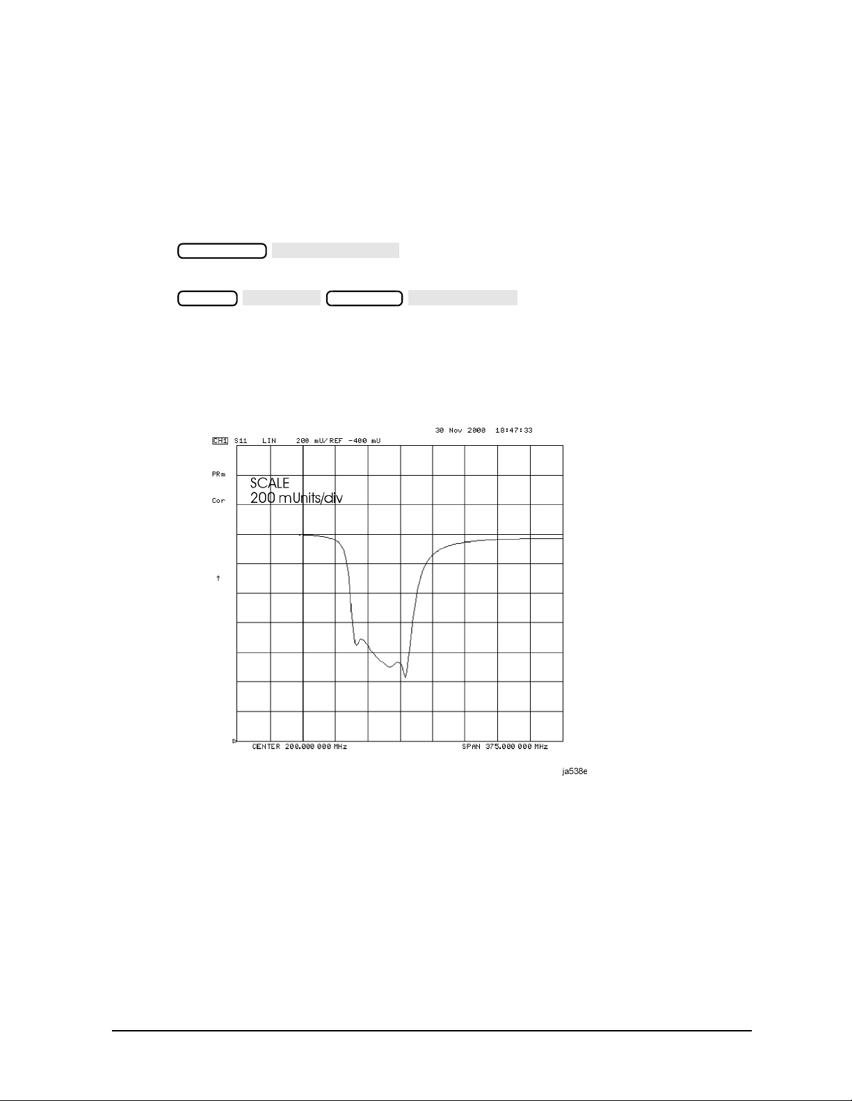
Measuring Reflection Coefficient
1. Press to recall the calibrated reflection measurement
Save/Recall
that you saved earlier in this procedure.
2. Press so the analyzer shows the same
Format
Scale Ref
data in terms of reflection coefficient, as shown in Figure 2-12.
The units “mU” displayed on the analyzer are “milli-units,” where “units” or “U” is used
to indicate that the parameter is unitless (as opposed to dB in log magnitude format).
For example, 200 mUnits = 0.2.
Figure 2-12 Example Reflection Coefficient Measurement Trace
Chapter 2 2-19
Page 53

Quick Start: Learning How to Make Measurements
SWR
AUTO SCALE
Learning to Make Reflection Measurements
Measuring Standing Wave Ratio (SWR)
Press so the analyzer shows the same data in
Format
Scale Ref
terms of standing-wave-ratio (SWR), as shown in Figure 2-13.
Now the analyzer shows the measurement data in the unitless measure of SWR where
SWR = 1 (perfect match) at the bottom of the display.
Figure 2-13 Example Standing-Wave-Ratio Measurement Trace
2-20 Chapter2
Page 54

Quick Start: Learning How to Make Measurements
POLAR
AUTO SCALE
MARKER MODE MENU
POLAR MKR MENU
LIN MKR
LOG MKR
Re/Im MKR
Learning to Make Reflection Measurements
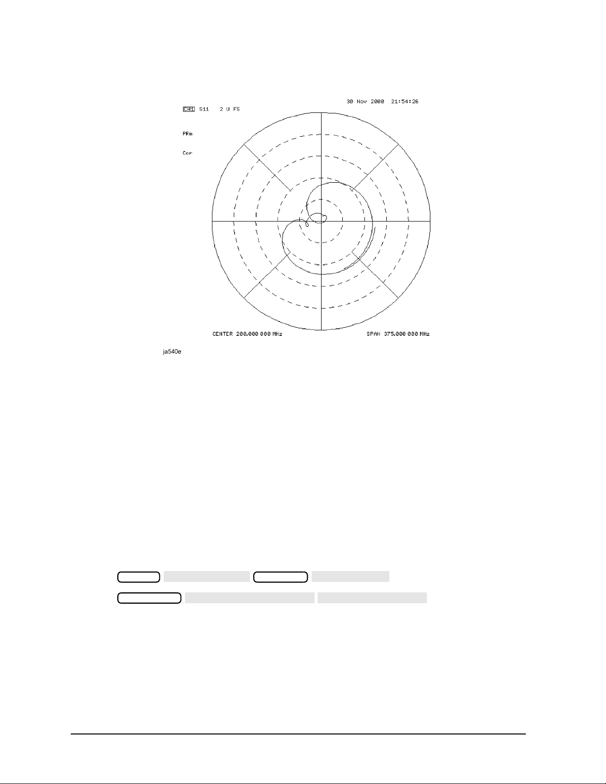
Measuring S11 and S22 or Reflection in a Polar Format.
1. Press .
2. Press to reposition the trace, as shown in Figure 2-14.
The analyzer shows the results of an S
Format
Scale Ref
or reflection measurement with each point on
11
the polar trace corresponding to a particular value of both magnitude and phase. The
center of the circle represents a coefficient (Γ) of 0, (that is, a perfect match or no
reflected signal). The notation 2U FS or 2 units full scale indicates that the
outermost circumference of the scale shown in Figure 2-14 represents ρ = 2.00, or 200%
reflection. The phase angle is read directly from this display. The 3 o'clock position
corresponds to zero phase angle, (that is, the reflected signal is at the same phase as the
incident signal). Phase differences of 90°, 180°, and −90° correspond to the 12 o'clock, 9
o'clock, and 6 o'clock positions on the polar display, respectively.
3. Press .
Marker Fctn
4. Turn the front panel knob to position the marker at any desired point on the trace, then
read the frequency, linear magnitude and phase in the upper right-hand corner of the
display.
• Choose if you want the analyzer to show the linear magnitude and the
phase of the marker.
• Choose if you want the analyzer to show the logarithmic magnitude and
the phase of the active marker. This is useful as a fast method of obtaining a reading
of the log-magnitude value without changing to log-magnitude format.
• Choose if you want the analyzer to show the values of the marker as a
real and imaginary pair.
NOTE You can also enter the frequency of interest, from either the numeric keypad
or the optional attached keyboard, and read the magnitude and phase at that
point.
Chapter 2 2-21
Page 55
Quick Start: Learning How to Make Measurements
SMITH CHART
AUTO SCALE
MARKER MODE MENU
SMITH MKR MENU
Learning to Make Reflection Measurements
Figure 2-14 Example S11 or Reflection Measurement Trace in Polar Format
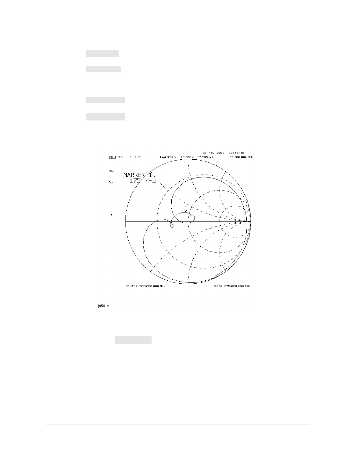
Measuring S
• Measuring Impedance
and S22 or Reflection in a Smith Chart Format.
11
The amount of power reflected from a device is directly related to the impedance of the
device and the measuring system. Each value of the reflection coefficient (Γ) uniquely
defines a device impedance; Γ = 0 only occurs when the device and analyzer impedance are
exactly the same. The reflection coefficient for a short circuit is: Γ = 1 ∠ 180°. Every other
value for Γ also corresponds uniquely to a complex device impedance, according to the
equation:
Z
= [(1 + Γ) / (1 −Γ)] × Z
L
0
where ZL is your test device impedance and Z0 is the measuring system's characteristic
impedance (usually 50Ω or 75Ω).
1. Press .
2. Press and turn the front
Format
Marker Fctn
Scale Ref
panel knob to read the resistive and reactive components of the complex impedance at
any point along the trace, as shown in Figure 2-15. Here the complex impedance is
6.4729 – j7.5569 Ω. This is the default Smith chart marker.
The marker annotation also gives the series inductance or capacitance (132.87 pF in
this example). The complex impedance is capacitive in the bottom half of the Smith
chart display and is inductive in the top half of the display.
2-22 Chapter2
Page 56
Quick Start: Learning How to Make Measurements
LIN MKR
LOG MKR
Re/Im MKR
R+ jX MKR
G+ jB MKR
Learning to Make Reflection Measurements
• Choose if you want the analyzer to show the linear magnitude and the
phase of the reflection coefficient at the marker.
• Choose if you want the analyzer to show the logarithmic magnitude and
the phase of the reflection coefficient at the active marker. This is useful as a fast
method of obtaining a reading of the log magnitude value without changing to log
magnitude format.
• Choose if you want the analyzer to show the values of the reflection
coefficient at the marker as a real and imaginary pair.
• Choose (the default marker format) to show the real and imaginary
parts of the device impedance at the marker. Also shown is the equivalent series
inductance or capacitance (the series resistance and reactance, in ohms).
Figure 2-15 Example Impedance Measurement Trace
• Measuring Admittance
To change the display to an inverse Smith chart graticule and the marker information to
read admittance, press .
As shown in Figure 2-16, the marker reads admittance data in the form G+jB, where G is
conductance and B is susceptance, both measured in units of Siemens (equivalent to mhos:
the inverse of ohms). Also shown is the equivalent parallel capacitance or inductance.
Chapter 2 2-23
Page 57

Quick Start: Learning How to Make Measurements
Learning to Make Reflection Measurements
Figure 2-16 Example Admittance Measurement Trace
2-24 Chapter2
Page 58
Quick Start: Learning How to Make Measurements
If You Encounter a Problem
If You Encounter a Problem
If you have difficulty when installing or using the analyzer, check the following list of
commonly encountered problems and troubleshooting procedures. If the problem that you
encounter is not in the following list, refer to additional troubleshooting sections in the
Service Guide.
Power-Up Problems
If the analyzer display does not light:
• Check that the power cord is fully seated in both the main power receptacle and the
analyzer power module.
• Check that the AC line voltage selector switch is in the appropriate position
(230 V/115 V) for your available power supply.
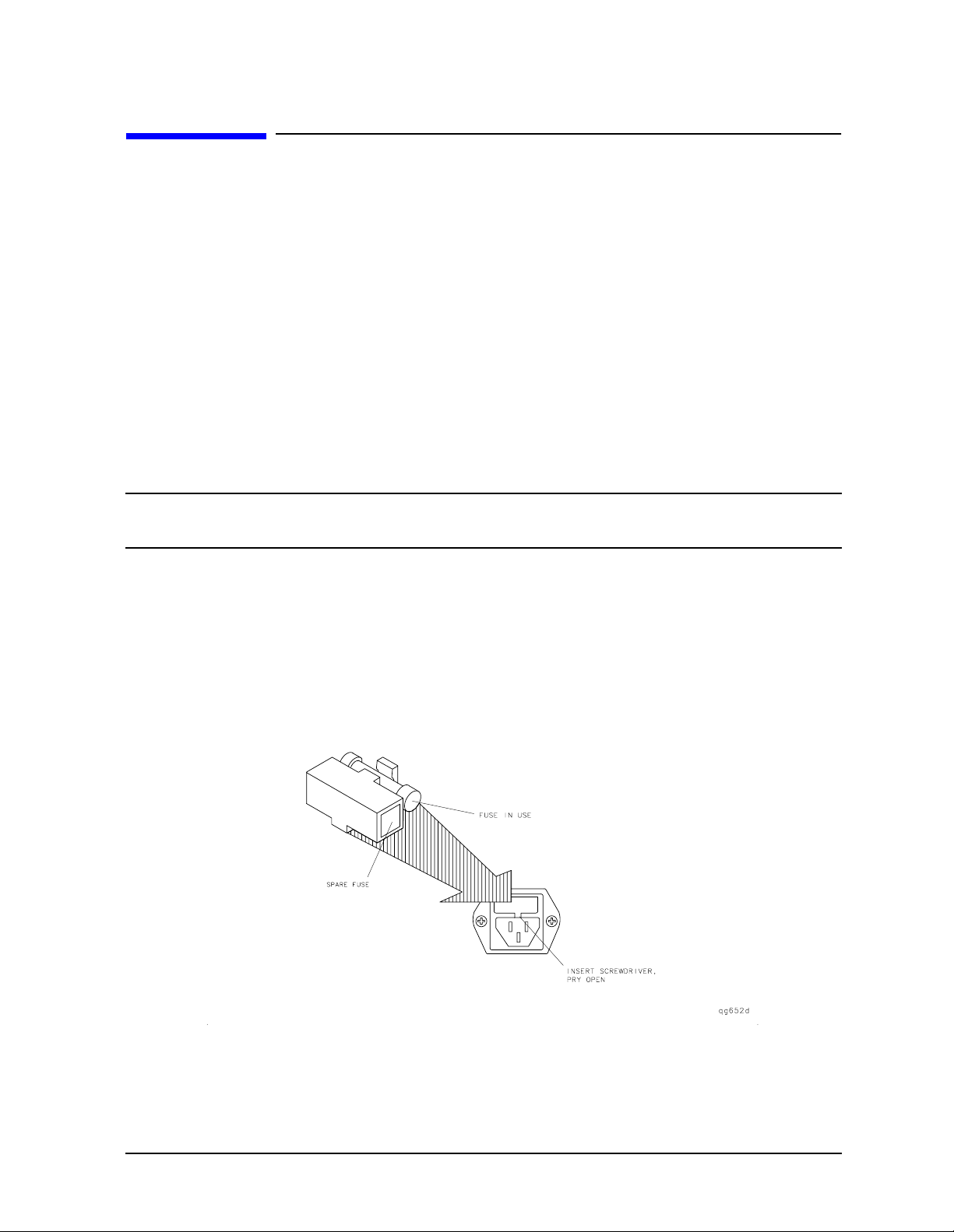
• Check that the analyzer AC line fuse is not open.
WARNING For continued protection against fire hazard, replace the fuse with
the same type and rating.
Refer to Figure 2-17 to remove the fuse from the power module. You can use a
continuity light or an ohmmeter to check the fuse. An ohmmeter should read very close
to zero ohms if the fuse is good. For 115V operation, use Fuse, T 5A 125V, UL listed/CSA
certified to 248 standard (part number 2110-1059). For 230V operation, use Fuse, T 4A
H 250V, built to IEC 127-2/5 standard (part number 2110-1036).
• Contact the nearest Agilent Technologies office for service, if necessary. A list of Agilent
Technologies sales and service offices is provided in Table 2-1 on page 2-28.
Figure 2-17 Line Fuse Removal and Replacement
Chapter 2 2-25
Page 59

Quick Start: Learning How to Make Measurements
SOURCE PWR ON off
If You Encounter a Problem
If the display lights, but the ventilation fan does not start:
❏ Check that the fan is not obstructed. To check the fan, follow these steps:
1. Switch the LINE power to the off position.
2. Check that the fan blades are not jammed.
❏ Contact the nearest Agilent Technologiesoffice for service, if necessary. A list of Agilent
Technologies sales and service offices is provided in Table 2-1 on page 2-28.
Data Entry Problems
If the data entry controls (keypad, knob, arrow keys) do not respond:
❏ Check that the ENTRY OFF function is not enabled.
The ENTRY OFF function is enabled after you press the key. To return to
Entry Off
normal entry mode, press any function key that has a numeric parameter associated
with it, for example, .
Start
❏ Check that none of the keys are stuck.
❏ Check that the selected function key accepts data.
For example, accepts data, but does not.
Scale Ref System
❏ Check that the analyzer's "R" GPIB STATUS light is not illuminated.
If the analyzer's "R" GPIB STATUS light is illuminated, a test sequence may be
running, or a connected computer controller may be sending commands or instructions
to, or receiving data from, the analyzer. Press if you want to return to LOCAL
Local
control.
If the parameter you are trying to enter is not accepted by the analyzer:
❏ Ensure that you are not attempting to set the parameter greater than or less than its
limit. Refer to the User's Guide for parameter limits.
No RF Output
If there is no RF signal at the front-panel port:
❏ Check that the signal at the test port is switched on.
1. Press and toggle to ON.
NOTE On ES models, it is possible to set the source power to come from PORT 2
❏ If you are applying external modulation (AM) to the analyzer, check the external
modulating signal or external gate/trigger signals for problems.
2-26 Chapter2
Power
instead of PORT 1, so you must check the power at the correct port. With
factory preset, the power comes from PORT 1.
Page 60

Quick Start: Learning How to Make Measurements
If You Encounter a Problem
CAUTION If the error message:
CAUTION: OVERLOAD ON INPUT X, POWER REDUCED
appears on the analyzer display, too much source power is being applied at
the input. In such a case, the input power will need to be reduced before the
source power will remain on.
❏ If phase-lock error messages appear on the analyzer display, check that the front panel
jumper is secure on the R CHANNEL connectors. If the jumper is secure and the error
messages still appear, contact your nearest Agilent Technologies office for service. A list
of Agilent Technologies sales and service offices is provided in Table 2-1 on page 2-28.
Chapter 2 2-27
Page 61

Quick Start: Learning How to Make Measurements
If You Encounter a Problem
Table 2-1 Agilent Technologies Sales and Service Offices
UNITED STATES
Instrument Support Center
Agilent Technologies
(800) 403-0801
EUROPEAN FIELD OPERATIONS
Headquarters
Agilent Technologies S.A.
150, Route du Nant-d’Avril
1217 Meyrin 2/ Geneva
Switzerland
(41 22) 780.8111
Great Britain
Agilent Technologies Ltd.
Eskdale Road, Winnersh
Triangle Wokingham,
Berkshire RG41 5DZ England
(44 118) 9696622
Headquarters
Agilent Technologies
3495 Deer Creek Rd.
Palo Alto, CA 94304-1316
USA
(415) 857-5027
Japan
Agilent Technologies Japan,
Ltd.
Measurement Assistance
Center
9-1, Takakura-Cho,
Hachioji-Shi,
Tokyo 192-8510, Japan
TEL (81) -426-56-7832
FAX (81) -426-56-7840
France
Agilent Technologies France
1 Avenue Du Canada
Zone D’Activite De Courtaboeuf
F-91947 Les Ulis Cedex
France
(33 1) 69 82 60 60
INTERCON FIELD OPERATIONS
Australia
Agilent Technologies Australia
Ltd.
31-41 Joseph Street
Blackburn, Victoria 3130
(61 3) 895-2895
Singapore
Agilent Technologies Singapore
(Pte.) Ltd.
150 Beach Road
#29-00 Gateway West
Singapore 0718
(65) 291-9088
Germany
Agilent Technologies GmbH
Agilent Technologies Strasse
61352 Bad Homburg v.d.H
Germany
(49 6172) 16-0
Canada
Agilent Technologies (Canada)
Ltd.
17500 South Service Road
Trans-Canada Highway
Kirkland, Quebec H9J 2X8
Canada
(514) 697-4232
Taiwan
Agilent Technologies Taiwan
8th Floor, H-P Building
337 Fu Hsing North Road
Taipei, Taiwan
(886 2) 712-0404
China
China Agilent Technologies
38 Bei San Huan X1 Road
Shuang Yu Shu
Hai Dian District
Beijing, China
(86 1) 256-6888
2-28 Chapter2
Page 62

Index
Numerics
3 dB bandwidth
measuring
6 dB bandwidth
measuring
A
active channel keys
location
admittance
measuring
Agilent Technologies Sales and
Service Offices
analyzer configuration
attaching cabinet flanges with
attaching cabinet flanges
attaching front handles
for bench top use
for rack mount use
option 1D5
standard
with printers or plotters
B
backing up EEPROM disk
bench top configuration
C
connectors
probe power source
R channel
D
definitions
magnitude of reflection
reflection coefficient
return loss (dB)
standing-wave-ratio (SWR)
disk drive location
disk eject button
display location
E
EEPROM backup disk
electrical and environmental
requirements
entry block location
F
front panel
, 2-10
, 2-11
, 2-3
, 2-23
, 2-28
, 1-9–1-19
front handles
without front handles
, 1-19
, 1-17
, 1-16
, 1-16
, 1-10
, 1-10
, 1-16
, 2-4
, 2-4
coefficient
, 2-14
, 2-14
, 2-14
2-14
, 2-3
, 2-3
, 2-3
, 1-26
, 1-7
, 2-4
, 1-5, 2-3
, 1-18
, 1-11
, 1-26
,
H
high stability frequency reference
configuration
I
impedance
measuring
insertion loss
measuring
installation
instrument state function block
keys
, 2-4
L
line switch
location
active channel keys
disk drive
disk eject button
display
, 2-3
entry block
instrument state function block
keys
line switch
PORT 1
PORT 2
Preset key
probe power source connectors
R channel connectors
REFLECTION port
response function block keys
Return key
softkeys
stimulus function block keys
TRANSMISSION port
M
making measurements
measurement procedure
choosing measurement
making a measurement
measuring a device
outputting measurement
measuring insertion loss with
O
operation
installed options
, 2-4
, 2-4
2-4
2-3
, 2-3
2-3
parameters
calibration
results
marker functions
, 1-20–1-25
, 1-10
, 2-22
, 2-8
, 1-2
, 2-3
, 2-3
, 2-3
, 2-3
, 2-4
, 2-4
, 2-3
, 2-4
, 2-4
, 2-4
,
, 2-3
,
, 2-4
, 2-1–2-24
, 2-5
, 2-5
, 2-5
, 2-5
, 2-5
, 2-10
, 1-21
operator’s check
self-test
testing reflection mode
testing transmission mode
operator’s check
out-of-band rejection
measuring
P
parts list
parts received
passband flatness
measuring
passband ripple
measuring
plotter configuration
polar format
measuring
PORT 1
location
PORT 2
location
Preset key
location
printer configuration
probe power connectors
location
problems, data entry
,
controls do not respond
parameters not accepted
problems, power-up
display does not light
display lights but fan does not
problems, RF output
no RF signal at front panel port
R
R channel connectors
location
rack mount configuration
rear panel
reflection measurements
admittance
choosing measurement
impedance
making a measurement
measuring in polar format
measuring in smith chart
measuringreflectioncoefficient
measuring return loss
, 1-22
, 2-4
, 2-4
, 2-4
, 2-4
start
, 2-26
2-26
, 2-4
, 1-6
2-14–2-24
parameters
calibration
format
2-19
, 1-23
, 1-25
, 1-24
, 1-23
, 2-12
, 1-4
, 2-13
, 2-13
, 1-11
, 2-21
, 1-11
, 2-26
, 2-26
, 2-26
, 2-25–2-26
, 2-25
, 2-26
,
, 1-16
,
, 2-23
, 2-15
, 2-22
, 2-16
, 2-21
, 2-22
,
, 2-17
Index 1
Page 63

Index
measuring standing wave ratio
(SWR)
results
, 2-4
1-7
, 2-3
, 2-3
, 2-20
, 2-17
, 2-18
, 2-3
, 2-17
, 2-28
, 1-3
, 2-22
, 2-22
, 2-3
, 2-20
measuring the device
outputting measurement
REFLECTION port
location
requirements
electrical and environmental
response function block keys
location
Return key, location
return loss
measuring
S
Sales and Service Offices
shipment, verifying
smith chart
smith chart format
measuring
softkeys, location
standard analyzer configuration
1-10
standing wave ratio (SWR)
measuring
stimulus function block keys
location
,
,
T
transmission measurements
2-6–2-13
3 dB bandwidth
6 dB bandwidth
choosing the measurement
parameters
insertion loss
making a measurement
calibration
measuring insertion loss with
marker functions
measuring the device
out-of-band rejection
outputting measurement
results
passband flatness
passband ripple
TRANSMISSION port
location
troubleshooting
V
verifying the shipment
, 2-4
, 2-10
, 2-11
, 2-6
, 2-8
, 2-7
, 2-10
, 2-8
, 2-12
, 2-9
, 2-13
, 2-13
, 2-25–2-27
, 1-3
,
2 Index
 Loading...