Agilent 89441A Operating Guide

Agilent Technologies 89410A/89441A Operator’s Guide

Agilent Technologies Part Number 89400-90038 For instruments with firmware version A.08.00 Printed in U.S.A.

This software and documentation is based in part on the Fourth Berkeley Software Distribution under license from The Regents of the University of California. We acknowledge the following individuals and institutions for their role in the development: The Regents of the University of California .

Portions of the TCP/IP software are copyright Phil Karn, KA9Q.

The Analyzer at a Glance

This illustration shows the Agilent 89441A Vector Signal Analyzer, which consists of two components: the IF section on top and the RF section on bottom. The IF section is the Agilent 89410A; the RF section is the Agilent 89431A. Note that you can order the 89431A to convert an 89410A into an 89441A (see Options and Accessories later in this manual).

Front Panel

1-A softkey’s function changes as different

menus are displayed. Its current function is determined by the video label to its left, on the analyzer’s screen.

2-The analyzer’s screen is divided into two

main areas. The menu area, a narrow column at the screen’s right edge, displays softkey labels. The data area, the remaining portion of the screen, displays traces and other data.

3-The POWER switch turns the analyzer on

and off. If you have an 89441A, you must turn on the power switches on both the top and bottom box.

4-Use a 3.5 inch flexible disk (DS,HD) in this

disk drive to save your work.

5-The KEYBOARD connector allows you to

attach an optional keyboard to the analyzer. The keyboard is most useful for writing and editing Agilent Instrument BASIC programs.

6- The SOURCE connector routes the

analyzer’s source output to your DUT. If you have an 89441A, the Source output from the IF section (top box) is connected to the RF section (bottom box). If the RF section has option AY8 (internal RF source), the SOURCE output connector on the RFsection is a type-N ; otherwise it is a BNC.

7-The EXT TRIGGER connector lets you

provide an external trigger for the analyzer.

8-The PROBE POWER connectors provides

power for various Agilent active probes.

9-The INPUT connector routes your test signal

or DUT output to the analyzer’s receiver. If you have an 89441A, the INPUT on the RF section (bottom box) is connected to the CHANNEL 1 input on the IF section (top box).

10-Use the DISPLAY hardkeys and their

menus to select and manipulate trace data and to select display options for that data.

11-Use the SYSTEM hardkeys and their

menus to control various system functions (online help, plotting, presetting, and so on).

12-Use the MEASUREMENT hardkeys and

their menus to control the analyzer’s receiver and source, and to specify other measurement parameters.

13-The REMOTE OPERATION hardkey and

LED indicators allow you to set up and monitor the activity of remote devices.

14-Use the MARKER hardkeys and their

menus to control marker positioning and marker functions.

15-The knob’s primary purpose is to move a

marker along the trace. But you can also use it to change values during numeric entry, move a cursor during text entry, or select a hypertext link in help topics

16-Use the Marker/Entry key to determine the

knob’s function. With the Marker indicator illuminated the knob moves a marker along the trace. With the Entry indicator illuminated the knob changes numeric entry values.

17-Use the ENTRY hardkeys to change the

value of numeric parameters or to enter numeric characters in text strings.

18-The optional CHANNEL 2 input connector

routes your test signal or DUT output to the analyzer’s receiver. For ease of upgrading, the CHANNEL 2 BNC connector is installed even if option AY7 (second input channel) is not installed.

For more details on the front panel, display the online help topic “Front Panel”. See the chapter “Using Online Help” if you are not familiar with using the online help index.

iii

This page left intentionally blank

Saftey Summary

The following general safety precautions must be observed during all phases of operation of this instrument. Failure to comply with these precautions or with specific warnings elsewhere in this manual violates safety standards of design, manufacture, and intended use of the instrument. Agilent Technologies, Inc. assumes no liability for the customer’s failure to comply with these requirements.

GENERAL

This product is a Safety Class 1 instrument (provided with a protective earth terminal). The protective features of this product may be impaired if it is used in a manner not specified in the operation instructions.

All Light Emitting Diodes (LEDs) used in this product are Class 1 LEDs as per IEC 60825-1.

ENVIRONMENTAL CONDITIONS

This instrument is intended for indoor use in an installation category II, pollution degree 2 environment. It is designed to operate at a maximum relative humidity of 95% and at altitudes of up to 2000 meters. Refer to the specifications tables for the ac mains voltage requirements and ambient operating temperature range.

BEFORE APPLYING POWER

Verify that the product is set to match the available line voltage, the correct fuse is installed, and all safety precautions are taken. Note the instrument’s external markings described under Safety Symbols.

GROUND THE INSTRUMENT

To minimize shock hazard, the instrument chassis and cover must be connected to an electrical protective earth ground. The instrument must be connected to the ac power mains through a grounded power cable, with the ground wire firmly connected to an electrical ground (safety ground) at the power outlet. Any interruption of the protective (grounding) conductor or disconnection of the protective earth terminal will cause a potential shock hazard that could result in personal injury.

FUSES

Only fuses with the required rated current, voltage, and specified type (normal blow, time delay, etc.) should be used. Do not use repaired fuses or short-circuited fuse holders. To do so could cause a shock or fire hazard.

DO NOT OPERATE IN AN EXPLOSIVE ATMOSPHERE

Do not operate the instrument in the presence of flammable gases or fumes.

DO NOT REMOVE THE INSTRUMENT COVER

Operating personnel must not remove instrument covers. Component replacement and internal adjustments must be made only by qualified service personnel.

Instruments that appear damaged or defective should be made inoperative and secured against unintended operation until they can be repaired by qualified service personnel.

WARNING The WARNING sign denotes a hazard. It calls attention to a procedure,

practice, or the like, which, if not correctly performed or adhered to, could result in personal injury. Do not proceed beyond a WARNING sign until the indicated conditions are fully understood and met.

Caution The CAUTION sign denotes a hazard. It calls attention to an operating

procedure, or the like, which, if not correctly performed or adhered to, could result in damage to or destruction of part or all of the product. Do not proceed beyond a CAUTION sign until the indicated conditions are fully understood and met.

Safety Symbols

Warning, risk of electric shock

Caution, refer to accompanying documents

Alternating current

Both direct and alternating current

Earth (ground) terminal

Protective earth (ground) terminal

Frame or chassis terminal

Terminal is at earth potential.

Standby (supply). Units with this symbol are not completely disconnected from ac mains when

this switch is off

vii

This page left intentally blank.

viii

Options and Accessories: Agilent 89410A

To determine if an option is installed, press [

System Utility

] [

option setup

]. Installed options are also listed on the analyzer’s rear panel. To order an option to upgrade your 89410A, order 89410U followed by the option number.

To convert your 89410A DC-10 MHz Vector Signal Analyzer to an 89441A DC-2650 MHz Vector Signal Analyzer, order an 89431A. To order an option when converting your 89410A to an 89441A, order 89431A followed by the option number.

IMPORTANT To convert older HP 89410A analyzers (serial numbers below 3416A00617),

contact your nearest Agilent Technologies sales and service office.

Option Description

Agilent 89410U Opt

Add Precision Frequency Reference AY5 — Add Vector Modulation Analysis and Adaptive Equalization AYA AYA Add Waterfall and Spectrogram AYB AYB Add Digital Video Modulation Analysis and Adaptive Equalization

AYH AYH

(requires option AYA and UFG or UTH) Add Enhanced Data rates for GSM Evolution (EDGE) (requires

B7A B7A

option AYA) Add Digital Wideband CDMA Analysis

B73 B73

(requires options AYA and UTH) Add Digital ARIB rev 1.0-1.2 W-CDMA Analysis (requires option

B79 B79

B73) Add 3GPP version 3.1 W-CDMA Analysis

080 080

(requires options AYA and UTH) Add Second 10 MHz Input Channel AY7 AY7 Extend Time Capture to 1 megasample AY9 AY9 Add 4 Megabyte Extended RAM and Additional I/O UFG (obsolete: order option UTH) Add 20 Megabyte Extended RAM and Additional I/O UTH UTH Add Advanced LAN Support (requires option UFG or UTH) UG7 UG7 Add Agilent Instrument BASIC 1C2 1C2 Add PC-Style Keyboard and Cable U.S. version 1F0 1F0 Add PC-Style Keyboard and Cable German version 1F1 1F1 Add PC-Style Keyboard and Cable Spanish version 1F2 1F2 Add PC-Style Keyboard and Cable French version 1F3 1F3 Add PC-Style Keyboard and Cable U.K. version 1F4 1F4 Add PC-Style Keyboard and Cable Italian version 1F5 1F5 Add PC-Style Keyboard and Cable Swedish version 1F6 1F6

Agilent 89430/ 89431A Opt

continued on next page...

Option Description 89410U Opt 89431A Opt

Add Front Handle Kit AX3 AX3 Add Rack Flange Kit AX4 AX4 Add Flange and Handle Kit AX5 AX5 Add Extra Manual Set OB1 OB1 Add Extra Instrument BASIC Manuals OBU OBU Add Service Manual OB3 OB3 Add Internal RF Source — AY8 Delete High Precision Frequency Reference — AY4 Add 50 - 75 Ohm Minimum Loss Pads — 1D7 Firmware Update Kit UE2 UE2

The accessories listed in the following table are supplied with the Agilent 89410A.

Supplied Accessories Part Number

Line Power Cable See Installation and

Verification Guide

Standard Data Format Utilities 5061-8056

Agilent Technologies 89410A/89441A

(see title page in manual)

Operator’s Guide

Agilent Technologies 89410A Getting

(see title page in manual)

Started Guide

Agilent Technologies 89410A Installation and Verification Guide (see title page in manual)

Agilent Technologies 89400-Series GPIB Command Reference (see title page in manual)

GPIB Programmer’s Guide (see title page in manual)

Agilent Technologies 89400-Series GPIB Quick Reference (see title page in manual))

Coax BNC(m)-to-coax BNC(m) connector (with option AY5) 1250-1499

The accessories listed in the following table are available for the Agilent 89410A.

Available Accessories Part Number

Agilent 89411A 21.4 MHz Down Converter Agilent 89411A

89400-Series Using Instrument BASIC Agilent 89441-90013

Instrument BASIC User’s Handbook Agilent E2083-90005

Spectrum and Network Measurements Agilent 5960-5718

Box of ten 3.5-inch double-sided, double-density disks Agilent 92192A

Active Probe Agilent 41800A

Active Probe Agilent 54701A

Active Divider Probe Agilent 1124A

Resistor Divider Probe Agilent 10020A

Differential Probe (requires Agilent 1142A) Agilent 1141A

Probe Control and Power Module Agilent 1142A

50 Ohm RF Bridge Agilent 86205A

Switch/Control Unit Agilent 3488A

High-Performance Switch/Control Unit Agilent 3235A

GPIB Cable - 1 meter Agilent 10833A

GPIB Cable - 2 meter Agilent 10833B

GPIB Cable - 4 meter Agilent 10833C

GPIB Cable - 0.5 meter Agilent 10833D

HP Printer or Plotter (contact your local

Hewlett-Packard sales representative)

Options and Accessories: 89441A

To determine if an option is installed, press [ options are also listed on the analyzer’s rear panel. To order an option for an Agilent 89441A analyzer, order Agilent 89441U followed by the option number.

Option Description Agilent 89441U Option

Add Internal RF Source AY8

Add High Precision Frequency Reference AYC

Add Vector Modulation Analysis and Adaptive Equalization AYA

Add Waterfall and Spectrogram AYB

Add Digital Video Modulation Analysis and Adaptive Equalization (requires options AYA and UFG or UTH)

Add Enh. Data rates for GSM Evol (EDGE) (requires option AYA) B7A

Add Digital Wideband CDMA Analysis (requires options AYA & UTH)

Add Digital ARIB 1.0-1.2 W-CDMA Analysis (requires option B73) B79

Add 3GPP v 3.1 W-CDMA Analysis (requires opts AYA & UTH) 080

Add Second 10 MHz Input Channel AY7

Extend Time Capture to 1 megasample AY9

Add 4 Megabyte Extended RAM and Additional I/O UFG (obsolete: order option UTH)

Add 20 megabyte Extended RAM and Additional I/O UTH

Add Advanced LAN Support (requires option UFG or UTH) UG7

Add Agilent Instrument BASIC 1C2

Add 50 - 75 Ohm Minimum Loss Pads 1D7

Add PC-Style Keyboard and Cable U.S. version 1F0

Add PC-Style Keyboard and Cable German version 1F1

Add PC-Style Keyboard and Cable Spanish version 1F2

Add PC-Style Keyboard and Cable French version 1F3

Add PC-Style Keyboard and Cable U.K. version 1F4

Add PC-Style Keyboard and Cable Italian version 1F5

Add PC-Style Keyboard and Cable Swedish version 1F6

Add Front Handle Kit AX3

Add Flange and Handle Kit AX5

Add Extra Manual Set OB1

Add Extra Instrument BASIC Manuals OBU

Add Service Manual OB3

System Utility

] [

AYH

B73

option setup

]. Installed

xii

Firmware Update Kit UE2

The accessories listed in the following table are supplied with the Agilent 89441A.

Supplied Accessories Part Number

Line Power Cable See Installation and

Verification Guide

Rear Panel Lock Foot Kit Agilent 5062-3999

BNC Cable - 12 inch Agilent 8120-1838

2 BNC Cables - 8.5 inch HP 8120-2682

Coax BNC(m)-to-coax BNC(m) Connector (deleted with option AY4) Agilent 1250-1499

Type N-to-BNC Adapter (2 with option AY8) Agilent 1250-0780

Serial Interface Interconnect Cable Agilent 8120-6230

Interconnect Cable EMI Suppressor Agilent 9170-1521

Standard Data Format Utilities Agilent 5061-8056

Agilent 89410/89441A Operator’s Guide (see title page in manual)

Agilent Technologies 89441A Getting Started Guide (see title page in manual)

Agilent Technologies 89441A Installation and Verification Guide (see title page in manual)

Agilent Technologies 89400-Series GPIB Command Reference (see title page in manual)

GPIB Programmer’s Guide (see title page in manual)

Agilent Technologies 89400-Series GPIB Quick Reference (see title page in manual)

xiii

The accessories listed in the following table are available for the Agilent 89441A.

Available Accessories Part Number

Agilent 89411A 21.4 MHz Down Converter Agilent 89411A

89400-Series Using Instrument BASIC Agilent 89441-90013

Instrument BASIC User’s Handbook Agilent E2083-90005

Spectrum and Network Measurements Agilent 5960-5718

Box of ten 3.5-inch double-sided, double-density disks Agilent 92192A

Active Probe Agilent 41800A

Active Probe Agilent 54701A

Active Divider Probe Agilent 1124A

Resistor Divider Probe Agilent 10020A

Differential Probe (requires Agilent 1142A) Agilent 1141A

Probe Control and Power Module Agilent 1142A

50 Ohm RF Bridge Agilent 86205A

Switch/Control Unit Agilent 3488A

High-Performance Switch/Control Unit Agilent 3235A

GPIB Cable - 1 meter Agilent 10833A

GPIB Cable - 2 meter Agilent 10833B

GPIB Cable - 4 meter Agilent 10833C

GPIB Cable - 0.5 meter Agilent 10833D

HP Plotters and Printers (contact your local

Hewlett-Packard sales representative)

xiv

Notation Conventions

Before you use this book, it is important to understand the types of keys on the front panel of the analyzer and how they are denoted in this book.

Hardkeys Hardkeys are front-panel buttons whose functions are always the same.

Hardkeys have a label printed directly on the key. In this book, they are printed like this: [

Hardkey

Softkeys Softkeys are keys whose functions change with the analyzer’s current menu selection. A softkey’s function is indicated by a video label to the left of the key (at the edge of the analyzer’s screen). In this book, softkeys are printed like this: [

Toggle Softkeys Some softkeys toggle through multiple settings for a parameter. Toggle softkeys have a word highlighted (of a different color) in their label. Repeated presses of a toggle softkey changes which word is highlighted with each press of the softkey. In this book, toggle softkey presses are shown with the requested toggle state in bold type as follows: “Press [

Shift Functions In addition to their normal labels, keys with blue lettering also have a shift function. This is similar to shift keys on an pocket calculator or the shift function on a typewriter or computer keyboard. Using a shift function is a two-step process. First, press the blue [ display). Then press the key with the shift function you want to enable. Shift function are printed as two key presses, like this: [

Shift

key name on

] [

Shift Function

]” means “press the softkey [

] key (at this point, the message “shift” appears on the

Shift

]

key name

softkey

] until the selection on is active.”

Numeric Entries Numeric values may be entered by using the numeric keys in the lower right hand ENTRY area of the analyzer front panel. In this book values which are to be entered from these keys are indicted only as numerals in the text, like this: Press 50, [

Ghosted Softkeys A softkey label may be shown in the menu when it is inactive. This occurs when a softkey function is not appropriate for a particular measurement or not available with the current analyzer configuration. To show that a softkey function is not available, the analyzer ‘’ghosts’’ the inactive softkey label. A ghosted softkey appears less bright than a normal softkey. Settings/values may be changed while they are inactive. If this occurs, the new settings are effective when the configuration changes such that the softkey function becomes active.

enter

]

This page left intentionally blank.

xvi

In This Book

This book, “Agilent 89410A/Agilent89441A Operator’s Guide”, is designed to advance your knowledge of the Agilent 89410A and Agilent 89441A Vector Signal Analyzers. You should already feel somewhat comfortable with this analyzer, either through previous use or through performing the tasks in either product’s Getting Started Guide.” The book consists of both measurement tasks and concepts.

Measurement tasks

Measurement tasks provide step-by-step examples of how to perform specific tasks with your Agilent 89410A or Agilent 89441A Vector Signal Analyzer. These tasks may be similar to measurements you wish to make and you can modify them to meet your own needs. Even if these tasks are not specifically related to your measurement needs, you may find it helpful to perform the tasks anyway—they only take a few minutes each—since they will help you become familiar with many of your analyzer’s features.

Concepts

The concepts section provides you with a conceptual overview of the Agilent 89410A and Agilent 89441A and their essential features. This section assumes that you are already familiar with basic measurement concepts and is helpful in understanding the similarities and differences between the Agilent 89400 series analyzers and other analyzers you may have used. The concepts are also essential if you want to make the best use of the analyzer’s features.

To Learn More About the Agilent 89410A and Agilent 89441A

You may need to use other books in the Agilent 89400 series manual set. See the “Documentation Roadmap” at the end of this book to learn what each book contains.

xvii

This page left intentionally blank.

xviii

1 Demodulating an Analog Signal

To perform AM demodulation 1-2

To perform PM demodulation 1-4

To perform FM demodulation 1-6

2 Measuring Phase Noise

To measure phase noise 2-2

Special Considerations for phase noise measurements: 2-3

3 Characterizing a Transient Signal

To set up transient analysis 3-2

To analyze a transient signal with time gating 3-4

To analyze a transient signal with demodulation 3-5

4 Making On/Off Ratio Measurements

To set up time gating 4-2

To measure the on/off ratio 4-4

5 Making Statistical Power Measurements

To display CCDF 5-2

To display peak, average, and peak/average statistics 5-4

6 Creating Arbitrary Waveforms

To create a waveform using a single, measured trace 6-2

To create a waveform using multiple, measured traces 6-4

To create a short waveform using ASCII data 6-6

To create a long waveform using ASCII data 6-8

To create a contiguous waterfall or spectrogram display 6-10

To create a fixed-length waterfall display 6-12

To determine number of samples and ∆t 6-14

To output the maximum number of samples 6-15

xix

7 Using Waterfall and Spectrogram Displays (Opt. AYB)

To create a test signal 7-2

To set up and scale a waterfall display 7-4

To select a trace in a waterfall display 7-6

To use markers with waterfall displays 7-8

To use buffer search in waterfall displays 7-10

To set up a spectrogram display 7-11

To enhance spectrogram displays 7-12

To use markers with spectrogram displays 7-14

To save waterfall and spectrogram displays 7-15

To recall waterfall and spectrogram displays 7-16

8 Using Digital Demodulation (Opt. AYA)

To prepare a digital demodulation measurement 8-2

To demodulate a standard-format signal 8-4

To select measurement and display features 8-5

To set up pulse search 8-6

To set up sync search 8-8

To select and create stored sync patterns 8-9

To demodulate and analyze an EDGE signal 8-10

To troubleshoot an EDGE signal 8-12

To demodulate and analyze an MSK signal 8-14

To demodulate a two-channel I/Q signal 8-16

9 Using Video Demodulation

(Opt. AYH)

To prepare a VSB measurement 9-2

To determine the center frequency for a VSB signal 9-4

To demodulate a VSB signal 9-6

To prepare a QAM or DVB QAM measurement 9-8

To demodulate a QAM or DVB QAM signal 9-10

To select measurement and display features 9-12

To set up sync search (QAM only) 9-13

To select and create stored sync patterns (QAM only) 9-14

To demodulate a two-channel I/Q signal 9-15

10 Analyzing Digitally Demodulated Signals (Options

AYA and AYH)

To demodulate a non-standard-format signal 10-2

To use polar markers 10-4

To view a single constellation state 10-5

To locate a specific constellation point 10-6

To use X-axis scaling and markers 10-7

To examine symbol states and error summaries 10-8

To view and change display state definitions 10-10

To view error displays 10-12

11 Creating User-defined Signals (Options AYA and

AYH)

To create an ideal digitally modulated signal 11-2

To check a created signal 11-4

To create a user-defined filter 11-6

12 Using Adaptive Equalization (Options AYA and AYH)

To determine if your analyzer has Adaptive Equalization 12-2

To load the multi-path signal from the Signals Disk 12-3

To demodulate the multi-path signal 12-4

To apply adaptive equalization 12-6

To measure signal paths 12-8

To learn more about equalization 12-10

13 Using Wideband CDMA (Options B73, B79, and 080)

To view a W-CDMA signal 13-2

To demodulate a W-CDMA signal 13-4

To view data for a single code layer 13-6

To view data for a single code channel 13-8

To view data for one or more slots 13-10

To view the symbol table and error parameters 13-12

To use x-scale markers on code-domain power displays 13-14

14 Using the LAN (Options UTH & UG7)

To determine if you have options UTH and UG7 14-2

To connect the analyzer to a network 14-3

To set the analyzer’s network address 14-4

To activate the analyzer’s network interface 14-5

To send GPIB commands to the analyzer 14-6

To select the remote X-Windows server 14-7

xxi

To initiate remote X-Windows operation 14-8

To use the remote X-Windows display 14-9

To transfer files via the network 14-10

15 Using the Agilent 89411A Downconverter

Connection and setup details for the Agilent 89411A 15-4

Calibration 15-8

16 Extending Analysis to 26.5 GHz with 20 MHz

Information Bandwidth

Overview 16-2

System Description 16-3

Agilent 89410A Operation 16-5

HP/Agilent 71910A Operation 16-5

Mirrored Spectrums 16-6

IBASIC Example Program 16-6

System Configuration 16-7

Agilent 89410A Configuration 16-7

HP/Agilent 71910A Configuration 16-8

System Connections 16-10

Operation 16-13

Controlling the Receiver 16-14

Changing Center Frequency 16-14

Setting the Mirror Frequency Key 16-14

Changing the Reference Level 16-14

Resolution Bandwidth 16-16

DC Offset and LO Feedthrough 16-16

Calibrating the System 16-17

Calibration Methods 16-18

DC Offset 16-19

Channel Match 16-20

IQ Gain, Delay Match 16-20

Quadrature 16-22

17 Choosing an Instrument Mode

Why Use Scalar Mode? 17-2

Why Use Vector Mode? 17-4

Why Use Analog Demodulation Mode? 17-6

The Advantage of Using Multiple Modes 17-7

Scalar—the big picture 17-7

xxii

Vector—the important details 17-7

Analog Demodulation—another view of the details 17-7

Instrument Mode? Measurement Data? Data Format? 17-8

Instrument modes 17-8

Measurement data 17-8

Data format 17-8

Unique Capabilities of the Instrument Modes 17-9

18 What Makes this Analyzer Different?

Time Domain and Frequency Domain Measurements 18-2

The Y-axis (amplitude) 18-3

The X-axis (frequency) 18-3

What are the Different Types of Spectrum Analyzers? 18-4

Swept-tuned spectrum analyzers 18-4

Real-time spectrum analyzers 18-5

Parallel-filter analyzers 18-5

FFT analyzers 18-6

The Difference 18-8

Vector mode and zoom measurements 18-8

Stepped FFT measurements in Scalar mode 18-9

19 Fundamental Measurement Interactions

Measurement Resolution and Measurement Speed 19-2

Resolution bandwidth 19-2

Video filtering 19-3

Frequency span 19-3

Bandwidth coupling 19-4

Flexible bandwidth mode 19-4

Display resolution and frequency span 19-5

Windowing 19-6

General 19-6

Windows used with this analyzer 19-6

Enhancing the Measurement Speed 19-8

Digital storage 19-9

Zero response and DC measurements 19-9

Special Considerations in Scalar Mode 19-10

Sweep time limitations 19-10

Stepped measurements 19-10

The relationship between frequency resolution and display resolution 19-11

xxiii

Resolution bandwidth limitations 19-11

What is a detector and why is one needed 19-12

Manual sweep 19-13

Special Considerations in Vector Mode 19-14

Time data 19-15

The time record 19-16

Why is a time record needed? 19-16

Time record, span and resolution bandwidth 19-17

Measurement speed and time record length 19-17

How do the parameters interact? 19-18

Time record length limitations 19-19

Time record processing 19-20

20 Analog Demodulation Concepts

What is Analog Demodulation? 20-2

Applications 20-2

Using analog demodulation for zero span measurements 20-2

How Does Analog Demodulation Work in the Agilent 89400 Series Analyzer? 20-3

Special Considerations for Analog Demodulation 20-4

Time Correction and Analog Demodulation 20-5

The Importance of Span Selection 20-6

Including all important signal data 20-6

Checking for interfering signals 20-7

The Importance of Carrier Identification 20-8

Auto carrier with AM demodulation 20-8

Auto carrier with PM demodulation 20-8

Auto carrier with FM demodulation 20-8

Special considerations for auto carrier use 20-8

AM Demodulation Specifics 20-9

The algorithm 20-9

PM Demodulation Specifics 20-10

The algorithm 20-10

Auto carrier off 20-10

Auto carrier on 20-10

FM Demodulation Specifics 20-12

xxiv

The algorithm 20-12

Interactions with other features 20-13

Choosing trigger type with analog demodulation 20-13

Using gating and averaging with analog demodulation 20-13

Two-channel measurements and analog demodulation 20-13

21 Gating Concepts

What is Time Gating? 21-2

How Does it Work? 21-4

Important Concepts 21-5

Parameter Interactions 21-6

22 Digital Demodulation Concepts (Opt. AYA)

Overview 22-2

What you learn in this chapter 22-2

If you need background references 22-2

What this analyzer does 22-2

Measurement Flow 22-4

General block diagram 22-4

Digital Demodulator Block diagram (except FSK) 22-5

Digital Demodulator Block diagram: FSK 22-6

Measurement management 22-8

Measurement and display choices 22-8

Carrier locking 22-9

I-Q measured signal 22-10

I-Q reference signal 22-10

Special considerations for FSK demodulation 22-10

Parameter interactions 22-11

Span considerations 22-11

Data size considerations 22-12

Resolution bandwidth 22-12

Display limitations 22-12

Feature Availability in Digital Demod 22-13

Special considerations for sync search 22-14

Special considerations for pulsed signals 22-15

Speed and resolution considerations 22-16

Maximizing speed - measurement and display 22-16

Maximizing resolution 22-16

Filtering 22-17

General information 22-17

xxv

Filter choices for the measured and reference signals 22-17

Square-root raised cosine filters 22-18

Raised cosine filters 22-18

Gaussian filter 22-19

Low pass filter (for FSK) 22-19

User defined filters 22-19

IS-95 Filters 22-20

EDGE Filter 22-21

EDGE (winRC) Filter 22-21

23 Video Demodulation Concepts (Opt. AYH)

Overview 23-2

What you learn in this chapter 23-2

What option AYH does 23-2

Measurement Flow 23-3

General block diagram 23-3

Digital demodulator block diagram: QAM and DVB QAM 23-4

Digital demodulator block diagram: VSB 23-6

Measurement management 23-7

Measurement and display choices 23-7

Carrier locking (all except VSB) 23-8

Carrier locking and pilot search: VSB 23-9

Input Range 23-10

I-Q measured signal 23-10

I-Q reference signal 23-10

Parameter interactions 23-11

Data size considerations 23-11

Resolution bandwidth 23-11

Span considerations 23-12

Display limitations 23-13

Feature Availability in Video Demodulation 23-14

Special considerations for sync search 23-15

Special considerations for pulsed signals 23-16

Maximizing speed - measurement and display 23-16

Maximizing resolution 23-16

Filtering 23-17

General information 23-17

xxvi

24 Wideband CDMA Concepts (Options B73, B79, and

080)

Overview 24-2

What you learn in this chapter 24-2

What option B73 does 24-2

What option B79 does 24-3

What option 080 does 24-3

Measurement Flow 24-4

Setting up a W-CDMA Measurement 24-6

Signal Connections and Input Range 24-6

Frequency Span 24-7

Center Frequency 24-7

Scramble Code 24-7

Chip Rates, Code Layers, and Symbol Rates 24-8

Main Length 24-9

Filtering 24-9

Mirrored Spectrums 24-9

Time-Domain Corrections 24-9

Trigger Signal 24-10

Viewing Measurement Results 24-11

Code-Domain Power Displays 24-12

Time-Domain Displays 24-13

Time Gating 24-14

Parameter interactions 24-15

Data size considerations 24-15

Resolution bandwidth 24-15

Points Per Symbol 24-15

Feature Availability in W-CDMA 24-16

Troubleshooting W-CDMA Measurements 24-17

Index

Need Assistance?

Documentation Road Map

xxvii

Demodulating an Analog Signal

This chapter shows how to demodulate AM, FM, and PM signals using the Analog Demodulation instrument mode. In these examples the signals are provided by the Signals Disk which accompanies this documentation.

1-1

Demodulating an Analog Signal

To perform AM demodulation

The following procedure demonstrates demodulation using files on the signals disk that you load into the analyzer’s data registers and use as arbitrary source signals. The sample signal is a 5 MHz carrier that is amplitude modulated with a sine wave.

1. Initialize the analyzer:

Press [

89410A: [ 89441A: [

Press [

Instrument Mode

input section (0-10 MHz) RF section (0-10 MHz)

Preset

], [

2. Load the source signal file AMSIG.DAT into data register D1:

Insert the Signals Disk in the analyzer’s disk drive. Press [ Press [

Save/Recall

Return

Rotate the knob until the file AMSIG.DAT is highlighted. Press [

recall trace

], [

default disk

] (bottom softkey), [

], [

from file into D1

], then press:

receiver

], [

internal disk

catalog on

enter

] to select the internal disk drive.

]to display the files on the disk.

3. Connect the SOURCE output to the channel 1 INPUT.

4. Turn on the source and select arbitrary signal D1 (25 kHz sine modulating

5 MHz): Press [

Source

], [

source on

], [

source type

], [

arbitrary

]

5. Set the frequency span:

Press [

Frequency

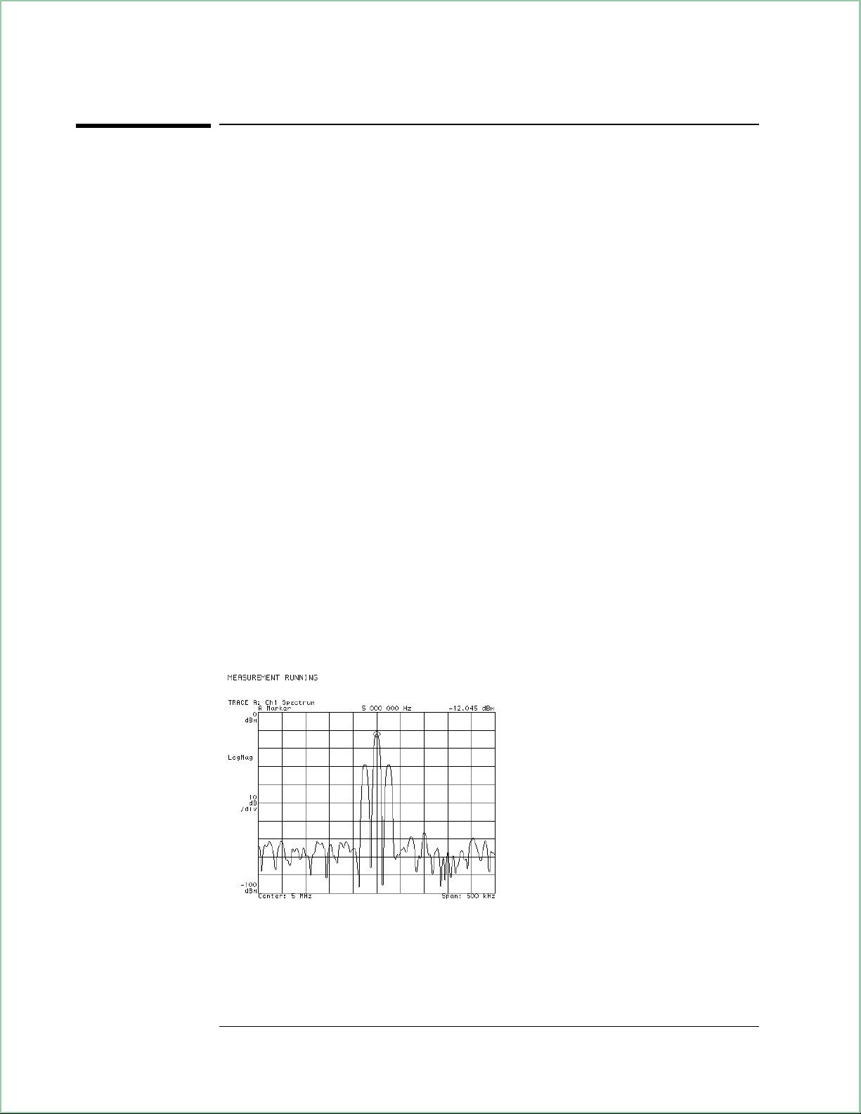
The display should now appear as shown below.

], [

], 500, [

span

kHz

Spectrum of the AM signal.

1-2

Demodulating an Analog Signal

6. Turn on AM demodulation and examine the recovered modulation signal:

Press [ [

Instrument Mode

Press [ Press [

Instrument Mode

demodulation setup

Auto Scale

], [demod type], [Analog Demodulation], [Return]).

], [

Analog Demodulation

], [

ch1 result

], [AM].

] (with option AYH, press

] to scale the display information, as shown below:

The AM demodulated spectrum.

7. Examine the recovered time-domain information:

Press [

Measurement Data

], [

main time

display the time data. Press [ Press [

Auto Scale Trigger

] to scale the display information.

], [

trigger type

], [

Recovered signal is volts as a function of time.

]([

internal source

main time ch1

] to stabilize the display.

] in a 2-channel analyzer) to

The span value sets the effective sample rate (∆t) and range of allowed

RBW values.

The RBW value determines the record length (T).

The number of measured points = T/∆t.

1-3

Demodulating an Analog Signal

To perform PM demodulation

The following procedure demonstrates PM demodulation using a file on the signals disk that you load into the analyzer’s data registers and use as an arbitrary source signal. The sample signal is a 5 MHz carrier that is phase modulated with a triangle wave.

1. Initialize the analyzer:

Press [

89410A: [

89441A: [

Press [

Instrument Mode

input section (0-10 MHz)

RF section (0-10 MHz)

Preset

], [

2. Load the source signal file PMSIG.DAT into data register D2:

Insert the Signals Disk in the analyzer’s disk drive. Press [ Press [

Save/Recall

Return

Rotate the knob until the file PMSIG.DAT is highlighted. Press [

recall trace

], [

default disk

] (bottom softkey), [

], [

from file into D2

], then press:

receiver

], [

internal disk

catalog on

enter

] to select the internal disk drive.

]to display the files on the disk.

3. Connect the SOURCE output to the channel 1 INPUT.

4. Turn on the source and select arbitrary signal D2

(a 25 kHz triangle wave modulating a 5 MHz carrier): Press [

Source

], [

source on

], [

source type

], [

arb data reg

], [D2], [

5. Set the frequency span:

Press [

Frequency

The display should now appear as shown below.

], [

], 500, [

span

kHz

Return

], [

arbitrary

Spectrum of the phase modulated signal.

1-4

Demodulating an Analog Signal

6. Turn on demodulation (PM) and examine the recovered modulation signal:

Press [ [

Instrument Mode

Press [ Press [

Instrument Mode

], [demod type], [Analog Demodulation], [Return]).

demodulation setup

Auto Scale

The display should now appear as shown below.

], [

Analog Demodulation

], [

ch1 result

], [PM].

] (with option AYH, press

] to scale the display information.

The PM demodulated spectrum.

7. Examine the recovered time-domain information:

Press [

Measurement Data

], [

main time

to display the time data. Press [ Press [ Press [

], [

Trigger Auto Scale

], [

Display

trigger type

] to scale the display information.

more display setup

], [

The display should now appear as shown below.

]([

internal source

], [

grids off

main time ch1

] to stabilize the display.

] in a 2-channel analyzer)

The recovered signal is in radians as a function of time.

1-5

Demodulating an Analog Signal

To perform FM demodulation

The following procedure demonstrates FM demodulation using a file on the signals disk that you load into the analyzer’s data registers and use as an arbitrary source signal. The sample signal is a 5 MHz carrier that is phase modulated with a triangle wave.

1. Initialize the analyzer:

Press [

89410A: [ 89441A: [

Press [

Instrument Mode

input section (0-10 MHz) RF section (0-10 MHz)

Preset

], [

2. Load the source signal file PMSIG.DAT into data register D2:

Insert the Signals Disk in the analyzer’s disk drive. Press [ Press [

Save/Recall

Return

Rotate the knob until the file PMSIG.DAT is highlighted. Press [

recall trace

], [

default disk

] (bottom softkey), [

], [

from file into D2

], then press:

receiver

], [

internal disk

catalog on

enter

] to select the internal disk drive.

]to display the files on the disk.

3. Connect the SOURCE output to the channel 1 INPUT.

4. Turn on the source and select arbitrary signal D2

(a 25 kHz triangle wave modulating a 5 MHz carrier): Press [

Source

], [

source on

], [

source type

], [

arb data reg

], [D2], [

5. Set the frequency span:

6. Press [

Frequency

The display should now appear as shown below.

], [

], 500, [

span

kHz

Return

], [

arbitrary

Spectrum of the phase modulated signal.

7. Select FM demodulation:

1-6

Demodulating an Analog Signal

Press [ [

Instrument Mode

Press [ Press [

Instrument Mode

demodulation setup

Auto Scale

], [demod type], [Analog Demodulation], [Return]).

], [

Analog Demodulation

], [

ch1 result

], [FM].

] (with option AYH, press

] to scale the display information.

The display should now appear as shown below.

The FM demodulated spectrum.

8. Examine the recovered signal:

Press [

Measurement Data

], [

main time

to display the time data. Press [ Press [ Press [

], [

Trigger Auto Scale

], [

Display

trigger type

] to scale the display information.

more display setup

], [

The display should now appear as shown below.

]([

internal source

], [

grids off

main time ch1

] to stabilize the display.

] in a 2-channel analyzer)

The recovered signal is in Hz as a function of time.

The recovered time data is displayed as a square wave because the relation between phase modulation and frequency modulation is a derivative and the derivative of a triangle wave is a square wave. Compare this recovered FM signal with the recovered PM signal in the previous task.

1-7

Measuring Phase Noise

This chapter demonstrates how to perform a phase noise measurement using a simulated input signal from a time capture signal.

2-1

Measuring Phase Noise

To measure phase noise

The following procedure demonstrates phase noise measurements using files on the signals disk that you load into the analyzer’s time-capture buffer. Then, instead of measuring data on the input, we analyze the data in the capture buffer. Reading data from the capture buffer is not normally part of measuring phase noise, but is necessary to document the procedure with simulated measurement data.

The settings that constitute a phase noise measurement:

Instrument Mode: PM demodulation

Measurement Data: PSD (power spectral density)

Data Format: x axis is log scale

Averaging, as required

1. Initialize the analyzer:

Press [

89410A: [ 89441A: [

Press [

Instrument Mode

input section (0-10 MHz) RF section (0-10 MHz)

Preset

], [

], then press:

receiver

2. If your analyzer has the optional second input channel installed, turn it off:

Press [

Input

], [

channel 2

], [

ch2 state off

3. Load the time-capture data into the capture buffer:

Insert the Signals Disk in the analyzer’s disk drive. Press [ Press [

Save/Recall

Return

Rotate the knob until the file CAPT.DAT is highlighted. Press [

recall more

Using time-captured data causes the analyzer to automatically select the capture buffer data instead of the input channel and sets the center frequency, span, and resolution bandwidth to those used when the data was captured. In a normal phase noise measurement you will set these parameters instead of loading captured data.

], [

default disk

], [

internal disk

] (bottom softkey), [

], [

recall capture buffer

catalog on

], [

enter

] to select the internal disk drive.

]to display the files on the disk.

] (takes about 2 minutes).

2-2

1. Select PM demodulation:

Press [

Mode

Press [

Instrument Mode

], [demod type], [Analog Demodulation], [Return]).

demodulation setup

], [

Analog Demodulation

], [

ch1 result

] (with option AYH, press [

], [PM].

2. Select PSD measurement data:

Press [

Measurement Data

], [

PSD

]([

PSD ch1

] for a 2-channel analyzer).

3. Set the x-axis scale to log:

Press [

Data Format

], [

x-axis log

4. Turn on averaging:

Press [

Average

], [

average on

], [

num averages

], 100, [

enter

], [

5. Run (or start) the measurement and scale the results:

Press [ Press [

Meas Restart Auto Scale

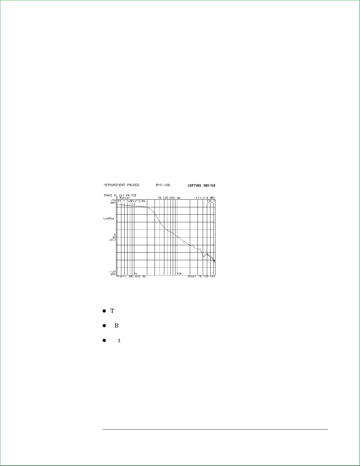
The display should now appear as shown below.

] to make the measurement.

] to scale the trace data.

fast avg on

Measuring Phase Noise

Instrument

Phase Noise Plot

Special Considerations for phase noise measurements:

This is a measurement of S0which is defined as the power in both sidebands of the phase noise. L

RBW must be small enough so that the low frequency portion of the log X-axis is valid. RBW should be less than the start frequency.

Note that the span in demodulation mode is one-half the span of the instrument.

is typically defined as the power in one sideband.

(f)

2-3

Characterizing a Transient Signal

This chapter demonstrates two methods of characterizing a transient signal. In this case you will characterize a simulated transmitter turn-on signal.

3-1

Characterizing a Transient Signal

To set up transient analysis

This procedure demonstrates several transient signal characterization methods. The signal is loaded from disk into a data register and selected as an arbitrary source signal. The signal simulates a transmitter turning on.

1. Select the baseband mode and initialize the analyzer:

Press [

Instrument Mode

89410A: [ 89441A: [ Press [

Preset

], [

input section (0-10 MHz) RF section (0-10 MHz)

], then press:

receiver

2. Load the source signal file XMITR.DAT into data register D1:

Insert the Signals Disk in the analyzer’s disk drive. Press [ Press [

Save/Recall

Return

], [

default disk

], [

internal disk

] (bottom softkey), [

catalog on

] to select the internal disk drive.

] to display the files on the disk. Rotate the knob until the file XMITR.DAT is highlighted. Press [

recall trace

], [

from file into D1

], [

enter

3. Connect the SOURCE output to the channel 1 INPUT.

4. Turn on the source and select arbitrary signal D1:

Press [

Source

], [

source on

], [

source type

], [

arbitrary

5. Select a window and increase the display resolution by increasing the number

of frequency points: Press [

Press [

ResBW/Window

], [

Return

], [

num freq pts

main window

], 801, [

], [

gaussian top

] (or use the increment key).

enter

]

6. Set the display to show spectrum and time information:

Press [ Press [

Display

],[

analyzer).

], [

Mea surement Data

2 grids

], [

main time

] (toggle to

ch1 for 2-channel

3-2

Characterizing a Transient Signal

7. Set the sweep and trigger:

Press [ Press [ Press [ The display should now appear as shown below.

Spectrum (top) and time domain representation (bottom) of transient signal.

], [

Trigger

], [

Sweep Auto Scale

trigger type

], [

single

], [

internal source

Pause|Single

] to simulate a “transient.”

3-3

Characterizing a Transient Signal

To analyze a transient signal with time gating

This procedure assumes that the steps in “To set up transient analysis” have been performed. If not, do so before continuing.

1. Turn on time gating, set the gate length, and set up the knob to move the gate:

Press [ Press the [

Time

], [gate on ], [gate length], 3, [us], [

Marker|Entry

] hardkey so that the knob’s “Entry” LED is on.

ch1 gate dly

2. Rotate the knob to move the gate over the very first part of the transient signal

appearing in the lower trace; see the plot below.

3. Set up the marker to show the movement of the spectrum’s peak:

Press [ Press [

], [

Marker Function

], [

Shift

], [

peak track

Marker⇒] (turns offset marker on and zeros it).

4. Now, move the time gate across the transient signal’s time display (by turning

the knob) and note the movement of the spectrum peak: Press [

Press [

Rotate the knob, moving the gate further to the right into the transient signal and stop long enough for the spectrum to update. Then move it again and stop. The reference marker (square) remains at the location of the “transient start up” making it easier to see the carrier movement as the regular marker (diamond) tracks the peak. Marker readouts in the display pictured below show that early in the transient there is as much as 1.00 MHz variation in carrier frequency.

], and make sure [

Time Marker|Entry

] if the knob’s “Entry” LED is not on.

ch1 gate dly

] is selected (if not, press it).

With time gating on, the spectrum shown (top) is that of the data inside the gate markers (bottom). In this case, moving the time gate across the time signal (bottom) shows that the carrier frequency varies with time (the spectral peak moves). We can use FM demod to show this, too. (grids were turned off in the illustration to highlight the gate markers.)

3-4

Characterizing a Transient Signal

To analyze a transient signal with demodulation

This procedure analyzes the frequency and amplitude variations of the transient signal with demodulation. It assumes that the steps in “To set up transient analysis” have been performed. If not, do so before beginning.

1. If you just finished the setup procedure, go to step 2 (don’t perform this step).

If you just finished the time gating analysis, go back to main time: Press [

2. Turn on FM demodulation:

Press [ [

Instrument Mode

Press [ Press [

3. Now rescale to examine the results:

Press [ Press [ The display should appear as shown below.

], [

Time

Instrument Mode

gate off

], [demod type], [

demodulation setup

Pause|Single

], [

] to simulate a transient and take data.

Auto Scale

Ref Lvl/Scale

]

], [

Analog Demodulation

], [

ch1 result

], [

Y per div

], [FM].

], 200, [

] (with option AYH, press

], [Return]).

], 3, [Hz].

exponent

FM demodulation analysis. The bottom trace shows the frequency variation in the transient signal. Comparing it with the time signal in the previous figure shows that demod results are meaningless during periods of no signal.

3-5

Characterizing a Transient Signal

4. Now we’ll look at the amplitude response of the signal with AM demodulation:

Press [ Press [

Instrument Mode Pause|Single

], [

demodulation setup

], [

ch1 result

], [AM].

5. Now scale both traces:

Press the blue [ on). Press [ The display should now appear as shown below.

Auto Scale

], [A]. Traces A and B should be active (both LEDs

Shift

] to automatically scale the active traces.

AM demodulation analysis (bottom trace). Note that there is more ringing (more cycles before settling) in the amplitude of the transient signal than was seen in the frequency analysis (compare bottom trace of this figure with that of FM demodulation in the previous figure)

3-6

Making On/Off Ratio Measurements

This chapter shows you how to measure the on/off ratio of a burst signal. This type of signal is typical in communication applications which use a burst carrier. You will use a signal from the Signals Disk to simulate a phase-modulated burst carrier.

4 - 1

Making On/Off Ratio Measurements

To set up time gating

1. Select the baseband mode and initialize the analyzer:

Press [

Instrument Mode

89410A: [ 89441A: [

Preset

input section (0-10 MHz) RF section (0-10 MHz)

2. Load a burst signal from the Signals Disk into a register and play it through the

source: Insert the Signals Disk in the internal disk drive.

Connect the SOURCE to the channel 1 INPUT. Press [ Press [

Rotate the knob to highlight PMBURST.DAT Press

Press [

Save/Recall

], [

Return

[recall trace

Source

], [

3. Select a window:

Press [

ResBW\Window

], [

receiver

], [

default disk

catalog on].

], [

from file into D1

source on], [source type

], [

main window

], then press:

], [

internal disk

], [

enter

], [

arbitrary

gaussian top

The display should now appear as below.

A 5 MHz burst carrier, phase-modulated with a 25 kHz signal.

4 - 2

Making On/Off Ratio Measurements

4. Turn on a second trace and configure it to display stable time data:

Press [ Press [ Press [ Press [

([

Press [

main time ch1

], [

Display Trigger

B Measurement Data

], [

2 grids trigger type

] for a 2-channel analyzer).

Auto Scale

], [

internal source

main time

]

5. Set up a gate to encompass the first burst:

Press [ Pre ss [ Rotate the knob to align the left gate marker with the beginning of the first burst. Press [ Rotate the knob to align the right gate marker with the end of the first burst.

], [

Time

Marker|Entry

gate length

gate on

]

], [

ch1 gate dly

] to turn on the Entry LED.

6. Turn off the grids to highlight the gate markers:

Press [ The display should now appear as below.

Display

], [

more display setup

], [

grids off]

The lower trace displays the time domain signal with a gate encompassing the first burst. The upper trace displays the frequency spectrum of the gated burst.

4 - 3

Making On/Off Ratio Measurements

To measure the on/off ratio

This assumes you have already set up time gating as in “To set up time gating.”

1. Turn on averaging:

], [

Shift

Time

average on].

], [

Marker

], [

ch1 gate dly

], [

Shift

], [

Marker⇒

Press [

Average

2. Turn on and zero the offset marker on the spectrum display:

Press [

3. Move the gate to the “off” portion of the time display:

Press [ Rotate the knob until the gate markers encompass the “off” portion of the signal.

The display should appear as below.

This measurement allows you to determine how much of the carrier leaks through to the off portion of a burst transmission and therefore establishes the dynamic range of the transmission system. In this particular example the dynamic range is low because of the noise inherent in playing a signal through the arbitrary source.

On the upper trace the offset marker is set at the “on” signal level. When the gate is moved to the “off” portion of the signal, the marker reading reflects the difference between the “on” portion and the “off” portion of the signal.

4 - 4

Making Statistical Power Measurements

This chapter shows you how to make statistical power measurements, such as CCDF (Complementary Cumulative Density Function), and peak, average, and peak-to-average statistical measurements.

5 - 1

Making Statistical Power Measurements

To display CCDF

This procedure shows you how to display the Complementary Cumulative Density Function (CCDF). The procedure uses the analyzer’s source to generate random noise and to display the CCDF of the random noise.

1. Preset the analyzer.

Press [

89410A: [ 89441A: [

Press [

Instrument Mode

input section (0-10 MHz) RF section (0-10 MHz)

Preset

], [

2. Select the Vector instrument mode.

Press [

Instrument Mode][Vector].

3. Connect the analyzer’s source to the channel 1 input.

4. Set the source level to 0 dBm, select random noise, and activate the source.

Press [ Press [ Select [

Source], [level] 0 dBm. source type], [random noise], [return]

source on].

], then press:

receiver

5. Set the range to 10 dBm.

Press [

Range] 10 dBm.

6. Enable time-domain corrections.

Press [

System Utility], [time domain cal on].

7. Set the frequency span to 5 MHz to band-limit the random noise signal (this

turns on the analyzer’s LO and zooms the time data). Press [Frequency], [span], 5 MHz.

8. Display the CCDF trace.

Press [

CCDF (complementary cumulative density function) is a statistical power-measurement that is the complement of CDF, as follows:

Measurement Data], [more choices], [CCDF ch1].

CDF: Probability (P CCDF: Probability (P

where:

= Instantaneous power

inst

= Average power

average

inst

≤ P

≥ P

average

)

5 - 2

Making Statistical Power Measurements

CCDF provides better resolution than CDF for low probability signals, especially when the y-axis is in log format. Presetting the analyzer automatically selects log format ([

Data Format], [magnitude log(dB)]).

The analyzer plots CCDF using units of % for the y-axis and power (dB) for the x-axis. Power on the x-axis is relative to the signal average power, so 0 dB is the average power of the signal. In other words, a marker reading that shows 12% at 2 dB means there is a 12% probability that the signal power will be 2 dB or more above the average power.

The analyzer computes CCDF using all samples in the current time record. Each successive measurement adds additional samples to the CCDF measurement. Pressing [

Measurement Restart] or changing most parameters

under the MEASUREMENT keygroup restarts the CCDF measurement.

Tips CCDF measurements operate on time data. By default, time data is

uncalibrated. Therefore, make sure you enable time-domain corrections as done in this procedure before making CCDF measurements.

For accurate CCDF measurements on burst signals, use triggering and time-gating to include only the burst in the CCDF measurement. Including the signal off-time degrades measurement accuracy. To learn how to use triggering and time gating, see “To set up time gating” in chapter 4.

When the y-axis is log format, the CCDF display shows two curves: the CCDF curve of your signal and the CCDF curve for an ideal band-limited Gaussian-noise signal.

In log format, the analyzer automatically plots the ideal curve (using the same color as the graticule) so you can compare it with that of your signal.

For comparison, this procedure set the span to 5 MHz to band-limit our random noise signal.

The CCDF measurement displays the number of samples used to compute CCDF (Cnt:) and the average power of your signal (Avg:).

CCDF of Random Noise

5 - 3

Making Statistical Power Measurements

To display peak, average, and peak/average statistics

This procedure shows you how to use features under [Marker Function]to display peak, average, and peak-to-average statistical power measurements. You can use these features to obtain the same results you get with CCDF measurements. Unlike CCDF measurements, you can display these statistical power measurements in any instrument mode as long as the active trace contains time-domain data. This is useful because these statistical power measurements give you a way to view power statistics using the analog, digital, video, and wideband CDMA instrument modes.

Use CCDF measurements for the power distribution of main time results. Use these statistical power measurements for demodulation results or results from math functions.

1. Perform the previous task.

The previous task generates the random noise signal used by this task. It also sets the input range and enables time-domain corrections.

2. Display time-domain data.

Press [

Measurement Data], [main time ch1].

3. Set the statistical percentage to 99.8%.

Press [

Marker Function], [peak/average statistics], [peak percent], 99.8%.

4. Select a statistical power measurement.

Press [

peak power].

5. Turn on the statistical power measurement.

Press [

In many applications, the instantaneous power of a signal can be treated as a random variable. Depending on the associated statistics, it may or may not make sense to define power in terms of an absolute value. Instead, power is defined in probablistic terms.

For example, you may determine that the instantaneous power of a given signal is less-than-or-equal to 3.5 dBm 99.8% of the time. In this case, you would say that the peak power is 3.5 dBm at a peak percent of 99.8%, or the peak power will be below 3.5 dBm 99.8% of the time. Alternatively, you could say that the instantaneous power will exceed 3.5 dBm 0.2% of the time (100% – 99.8% = 0.2%). You can represent this probability mathematically as:

statistics on],.

Probability (P Probability (P

≤ 3.5 dBm)=99.8% or, more generically:

inst

≤ P

)=Peak percent

peak

5 - 4

where:

= Instantaneous power

inst

= Peak power

peak

Peak percent = probability associated with P

peak

Making Statistical Power Measurements

Using the [Marker Function] hardkey, the analyzer lets you set the peak percent and then display peak, average, or peak-to-average statistical power for these configurations (otherwise the statistical softkeys are inactive):

The instrument mode is not Scalar.

The measurement contains time-domain data (x-axis is time).

The analyzer computes statistical power measurements using all samples in the current time record. Each successive measurement adds additional samples to the measurement. Pressing [

Measurement Restart] or changing most

parameters under the MEASUREMENT keygroup restarts the measurement.

num samples] softkey displays the number of samples used in the

The [ measurement.

Changing [

peak percent] or selecting a different statistical power computation

does not restart the measurement. For example, if you measure peak power and then select average power, the analyzer recomputes average power using all samples from the peak power measurement. This lets you view different statistics on the same data.

Important Statistical power measurements operate on time data. By default, time data is

uncalibrated. Therefore, make sure you enable time-domain corrections as done by step 1 in this procedure before making these measurements.

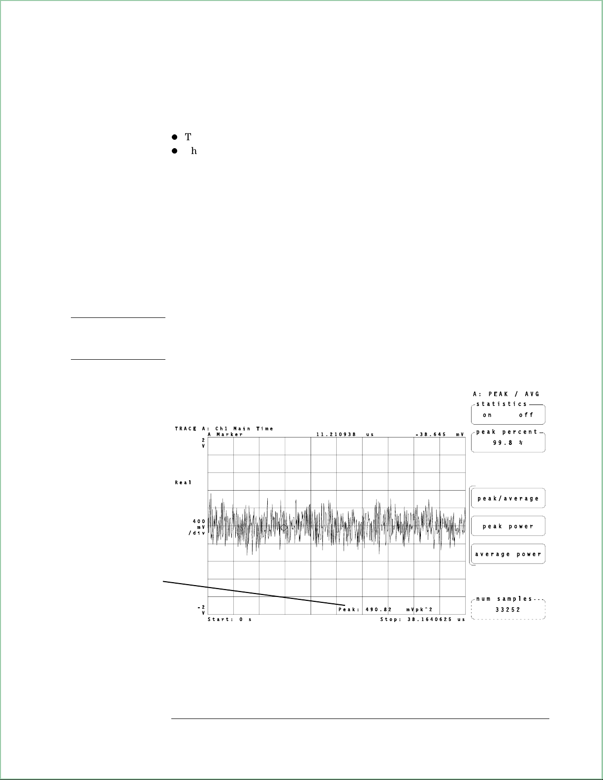
In this example, the peak power of this signal will be below this value

99.8% of the time.

Peak power statistical-power measurement

5 - 5

Creating Arbitrary Waveforms

This chapter shows you how to generate arbitrary waveforms using the analyzer’s arbitrary source. You can generate arbitrary waveforms that contain up to 16,384 samples of real or complex data. Under certain conditions, you can extend the arbitrary-source length to include up to 32,768 samples of real or complex data.

6-1

Creating Arbitrary Waveforms

To create a waveform using a single, measured trace

You use trace data to generate arbitrary waveforms. You can generate short or long waveforms. Short waveforms have up to 4096 samples of complex data or 8192 samples of real data. Long waveforms have more than 4096 samples of complex or 8192 samples of real data.

There are two ways of generating trace data. You can use measured data or you can use a computer program (such as MATLAB1) on your computer to generate trace data. This and the next task show you how to generate arbitrary waveforms using measured data. Subsequent tasks show you how to generate arbitrary waveforms using computer-generated data.

The steps below show you how to use a single, measured trace to create a short arbitrary waveform. See ‘’To create a waveform using multiple, measured traces’’ to learn how to create long arbitrary waveforms.

1. Initialize the analyzer and select the Vector instrument mode:

Press [

89410A: [

89441A: [ Press [ Press [

Instrument Mode

input section (0-10 MHz) RF section (0-10 MHz)

Preset

Instrument Mode

], [

], then press:

receiver

Vector

2. Connect your signal to the analyzer (this example uses the analyzer’s source to

provide a 1 MHz fixed-sine signal). Connect the SOURCE output to the CHANNEL 1 input.

Press [

Source

], [

source on

3. Select time-domain data.

Press [

Measurement Data], [main time].

4. Start the measurement:

Press [

Meas Restart

5. Save the trace data into a data register:

Press [

Save/Recall

], [

save trace

], [

into D1

6. Configure the arbitrary source to use your data:

1 MATLAB is a registered trademark of the The MathWorks, Inc.

6-2

Creating Arbitrary Waveforms

Press [

Source

], [

source type

], [

arbitrary

),[

arb data reg], [D1

]

The analyzer’s arbitrary source is now generating the same waveform as that displayed in the original trace.

The maximum number of samples in the source waveform is dependent on the sample rate used to create the arbitrary-source data. The maximum number of samples that the arbitrary source can output varies between 16,384 and 32,768 samples. For details, see ‘’To output the maximum number of samples’’ later in this chapter.

The analyzer’s arbitrary source requires time-domain data. Because of this, there are basically three steps to follow when using a single trace to create an arbitrary waveform:

1 Display the trace using time-domain measurement data. 2 Save the trace into a data register. 3 Turn on the arbitrary source and select the data register.

To create an arbitrary waveform, display your signal in the time domain and save the resulting trace to a data register. Then configure the arbitrary source to use the data register.

6-3

Creating Arbitrary Waveforms

To create a waveform using multiple, measured traces

Arbitrary waveforms that contain more than 4096 samples of complex or 8192 samples of real data are considered long waveforms. To create a long waveform using measured data, you must use multiple traces (a waterfall or spectrogram display).

1. Initialize the analyzer and select the Vector instrument mode:

Press [

Press [ Press [

Instrument Mode

89410A: [

89441A: [

Preset Instrument Mode

input section (0-10 MHz) RF section (0-10 MHz)

2. Connect your signal to the analyzer (this example uses the analyzer’s source to

provide a 1 MHz fixed-sine signal). Connect the SOURCE output to the CHANNEL 1 input.

Press [

Source

], [

source on

], then press:

receiver

Vector

3. Set the analyzer’s frequency span to include all components of your signal. If

possible, use a cardinal span to ensure the arbitrary source can output the maximum number of samples (for details, see ‘’To output the maximum number of samples’’ later in this chapter). Press [ Press [

Frequency span], 39.0625 kHz.

], [center], 1 MHz.

4. Create a contiguous waterfall or spectrogram display that contains

time-domain data. See ‘’To create a contiguous waterfall or spectrogram display.’’

5. Save the contiguous waterfall or spectrogram data into a data register:

Press [

Save/Recall

], [

save more

], [

save trace buffer

], [into D1].

6. View the data register contents on trace B (this step is optional):

Press [

B], [

Measurement Data

Press [Display], [waterfall setup], [waterfall on].

], [

data reg

], [

D1] .

7. Configure the analyzer to measure from the input channel instead of the

time-capture buffer: Press [

Instrument Mode

], [

measure from input

], [

remove capture

8. Turn on the arbitrary source:

Press [ Press [ Press [

], [

Source

arbitrary], [Return source on].

source type

], [

arb data reg], [D1

]

Return

The analyzer displays ‘’Loading arb source from register D1’’ and

‘’Arbritary Source length: XXX samples.’’

6-4

Creating Arbitrary Waveforms

9. Start the measurement and view the results:

Press [ The arbitrary source is now generating your signal.

Waterfall and spectrogram displays store trace data in the trace buffer. Both displays use the same trace buffer, therefore it doesn’t matter which display you use when you save the trace buffer. The [ determines the size of the trace buffer. For example, a buffer depth of 20 means the trace buffer can contain up to twenty traces, regardless of how many traces are displayed.

If the analyzer displays OUT OF MEMORY when you try to save data into a data register, you need to reconfigure the analyzer’s memory. You may want to press [ UFG. Option UFG adds an additional 4 MB of memory (and LAN capability) to your analyzer.

A], [Meas Restart].

buffer depth] softkey

System Utility], [options setup] to see if your analyzer has option

HINT A good way to increase the amount of memory available for data registers is to

reduce [ number of points in a trace and also reserves memory for other internal operations. Press [ change this parameter.

max freq points]. The value of this softkey determines the maximum

System Utility], [memory usage], [configure meas memory], [max freq points]to

The arbitrary source may not be able to use all data in the data register. The arbitrary source can use up to 16,384 samples of real or complex data. Under certain conditions, the arbitrary source can use up to 32,768 samples of real or complex data (see ‘’To output the maximum number of samples’’ later in this chapter).

In this example, the data register contains 20 traces. The value of [buffer depth] determines the number of traces saved to the data register.

6-5

Creating Arbitrary Waveforms

To create a short waveform using ASCII data

There are several computer programs that let you create arbitrary waveforms (such as MATLAB or MATRIXx2). This procedure shows you how to load a short, computer-generated waveform into the analyzer’s arbitrary source. Short waveforms contain 4096 complex or 8192 real points, or less.

1. Use your program to create a waveform that contains no more than 4096

complex or 8192 real points (for larger waveforms, see ‘’To create a long waveform using ASCII data’’).

2. Save your waveform as an ASCII file.

3. Convert your file from ASCII to SDF.

With the SDF utilities installed on your computer, type the following from a DOS prompt:

ASCTOSDF [/z:cf] /x:0, ∆t source_file destination_file

where: /z:cf specifies the center frequency (use with complex data).

/x:0 specifies the start time as 0 seconds.

∆t is the interval between samples.

source_file is the name of your ASCII file destination_file is the name of the SDF file.

4. Copy the SDF file to a 3.5" floppy disk.

5. Load the floppy disk into the analyzer and recall the SDF file into a data

Press [ Press [

Save/Recall

catalog on] and select your file. recall trace], [from file into D1].

], [

default disk

], [

internal disk

], [

Return

6. Configure the arbitrary source to use the data register.

Press [

Source

], [

source type

], [

arb data reg], [D1

]

Return

7. Turn on the arbitrary source.

Press [

The arbitrary source is now generating your waveform.

arbitrary

], [

Return

], [source on].

2 MATRIXx is a product of Integrated Systems, Inc.

6-6

Creating Arbitrary Waveforms

The analyzer stores trace data in Standard Data Format (SDF). Therefore, you must use the Standard Data Format utilities to convert your data to the SDF format recognized by the analyzer. For details about the SDF utilities, see the Standard Data Format Utilities: User’s Guide shipped with your analyzer.

The following paragraphs show you how the AMSIG.DAT file on the Signals Disk was created. This signal was created using MATLAB. It is an amplitude-modulated signal that uses a 25 kHz sinewave to modulate a 5 MHz carrier. The sample frequency is 25.6 MHz. Here are the equations and commands used to create this signal (> is the MATLAB prompt):

>t=0:1023; >x=t/1024*2*pi; >y=(sin(200*x)).*(.7+.2*sin(x ));R >save amsig.asc y /ascii >quit

where: t is a 1x1024 array of numbers from 0 to 1023.

x is a 1x1024 array of numbers from 0 to (almost) 2 pi. y is a 1x1024 array of numbers composing 200 cycles of a sinusoid

signal that is amplitude modulated by one cycle of a sinusoid

signal

that has an index of modulation of 0.7.

The MATLAB file was converted to SDF format using the ASCTOSDF utility, as follows:

ASCTOSDF /x:0,3.90625e-8 amsig.asc amsig.dat

where: /b: specifies the block size

/x: specifies the start time (or trigger delay) and ∆t.

∆ t =

sample frequency

25.6 MHz

= 3.90625 e

− 8

You can derive the frequency span using the following formula (use n =

2.56 since the ASCTOSDF command did not include the /z:cf argument):

span =

∆ t × n

where n =

1.28 for complex (zoom)data

2.56 for real (baseband) data

6-7

Creating Arbitrary Waveforms

To create a long waveform using ASCII data

There are several computer programs that let you create arbitrary waveforms (such as MATLAB or MATRIXx). This procedure shows you how to use a long, computer-generated waveform with the analyzer’s arbitrary source. Long waveforms have more than 4096 complex or 8192 real points.

1. Using your computer program, create your waveform and save it to an ASCII

file. Note the number of samples and the ∆t of your waveform.

2. Create a waterfall or spectrogram display that has the same number of samples

and ∆t as your waveform.

See “To create a fixed-length waterfall display.”

3. Using the results from the previous step, create a contiguous waterfall or

spectrogram display.

See “To create a contiguous waterfall or spectrogram display.”

4. Save the contiguous waterfall or spectrogram display (the trace buffer) to disk.

Press [ Press [

Save/Recall

save more

], [

default disk

], [

save trace buffer

], [

internal disk

], [into file].

], [

Return

5. Copy the trace-buffer file from disk onto your computer and put it in the same

directory as the ASCII file you created in step 1.

6. Use the sdfydata utility to replace the data in the trace_buffer file with data

from your ASCII file.

SDFYDATA sdf_file ASCII_file

where: sdf_file is the trace-buffer file.

ASCII_file is the ASCII file that you created in step 1.

6-8

Creating Arbitrary Waveforms

7. Load the modified trace-buffer file into one of the analyzer’s data registers.

On your computer, copy the modified trace-buffer file to floppy disk. Insert the disk in the analyzer’s disk drive. Press [ Press [

Save/Recall], [recall more], [catalog on] and select your file. recall trace buffer], [from file into D1].

8. Configure the arbitrary source to use the data register.

Press [

Source

], [

source type

], [

arb data reg], [D1

]

Return

9. Turn on the arbitrary source.

Press [

The analyzer stores trace data in Standard Data Format (SDF). You substitute trace data from a waterfall or spectrogram display using the sdfydata Standard Data Format (SDF) utility. This utility is one of several utilities included in the Standard Data Format Utilities: User’s Guide shipped with your analyzer. The sdfydata utility automatically converts the ASCII data to SDF format as it copies the ASCII data into the SDF file.

arbitrary], [Return], [source on].

For additional details about installing and using the SDF utilities, see the Standard Data Format Utilities: User’s Guide shipped with your analyzer.

6-9

Creating Arbitrary Waveforms

To create a contiguous waterfall or spectrogram display

Contiguous traces are needed when you use a waterfall or spectrogram display to generate an arbitrary-source waveform. You use waterfall or spectrogram displays to generate arbitrary waveforms that contain more than 4096 samples of complex data or 8192 samples of real data.

1. Prepare time-capture RAM for your signal:

Press [ Check [ Increase [

2. Fill time-capture RAM with your signal:

Press [

3. Set the overlap to 0%.

Press [

Instrument Mode], [capture setup buffer length] to verify that your signal will fit in time-capture RAM.

buffer length] if necessary.

fill buffer].

Time], [ovlp: avg off 0%].

]

4. Select time-domain data.

Press [

Measurement Data], [main time].

5. Select a waterfall or spectrogram display and set the buffer depth to 20.

Press [ Press [

Display], [waterfall setup], [waterfall on]. buffer depth 20].

6. Start the measurement:

Press [

Storing your signal in time-capture RAM and playing it back with 0% overlap ensures that the traces in a waterfall or spectrogram display are contiguous. To use waterfall or spectrogram data to drive the arbitrary source, you need contiguous traces to eliminate phase discontinuities in the arbitrary-source waveform. Make sure to display your data in the time domain since the arbitrary source requires time-domain data.

This procedure uses a buffer depth of 20 to accommodate all procedures in this chapter. Be sure to set the buffer depth according to your measurement needs.

Meas Restart

6-10

Creating Arbitrary Waveforms

To learn about waterfall and spectrogram displays, see ‘’Using Waterfall And Spectrogram Displays (Opt. AYB)’’ in the Operator’s Guide and see online help for the [

waterfall setup] and [spectrogram setup] softkeys.

This waterfall display was created with an elevation of 25 pixels and trace height of 30 pixels. Notice that the traces are contiguous (there is no phase discontinuity between traces). When looking at a waterfall display, remember that the top trace is the most recent trace, the trace before it is the previous trace, and so forth. Therefore, to see if a waterfall display is contiguous, you must piece the waveforms together from the bottom up.

Contiguous Waterfall Display With 20 Traces

6-11

Creating Arbitrary Waveforms

To create a fixed-length waterfall display

There are several computer programs that let you create arbitrary waveforms (such as MATLAB or MATRIXx). If the waveform is a long waveform (it contains more than 4096 complex points or 8192 real points), you must create a waterfall or spectrogram display on the analyzer, copy the waterfall or spectrogram data to your computer, and use the Standard Data Format (SDF) utilities to replace the waterfall or spectrogram data with the data from your computer program. The waterfall or spectrogram

data must have the same sample frequency, length, and ∆t (time-interval

between points) as your computer-generated waveform.

This procedure shows you how to create a waterfall or spectrogram display

that contains the number of samples and ∆t that you need. See ‘’To

create a long waveform using ASCII data’’ to learn how to perform the remaining steps.

This procedure configures the analyzer to create a waterfall display for a complex signal that has a sample frequency of 3.84 MHz and a total source length of 5ms. Substitute your values where necessary.

1. Initialize the analyzer and select the Vector instrument mode:

Press [

89410A: [

89441A: [ Press [ Press [

Instrument Mode

input section (0-10 MHz) RF section (0-10 MHz)

Preset

Instrument Mode

], [

], then press:

receiver

Vector

2. Set the rbw mode to arbitrary and rbw coupling to auto:

Press [

ResBW/Window

], [rbw mode arb], [rbw coupling auto], [Return].

3. Compute the total number of samples in the waveform:

Total Samples = 3.84

Msamples

sec

× 5 ms = 19,200 samples

4. Divide the total number of samples into N equal-length segments. Note that:

Each segment must contain an integer number of samples:

For real signals, each segment must have between 128 and 8192 samples.

For complex (zoom) signals, each segment must have between 64 and 4096

samples.

For this example, there are several possible solutions, such as:

10 segments of 1920 samples. 12 segments of 1600 samples.

20 segments of 960 samples.

6-12

Creating Arbitrary Waveforms

5. Set the number of frequency points for your signal. The number of frequency

points must be greater than the number of samples in a segment divided by

2.56 (real) or 1.28 (complex):

For 10 segments of 1920 samples:

For 12 segments of 1600 samples:

For 20 segments of 960 samples:

1920 samples

1.28

1600 samples

1.28

960 samples

1.28

= 1500 −−> Use 1601 freq. pts.

= 1250 −−> Use 1601 freq. pts.

= 750 −−> Use 801 freq. pts.

For this example, use 801 frequency points: Press [

ResBW/Window

], [num freq points], 801.

6. Set the frequency span to obtain the desired sample frequency. For real

signals, divide the sample frequency by 2.56; for complex signals, divide by 1.28:

Frequency span (complex)=

Press [

Frequency

], [span], 3, [MHz].

3.84 MHz

1.28

= 3 MHz

7. Set the time-record length equal to the length of one segment:

Length of one segment =

Press [Time], [main length], 250 [µ s].

960 samples

3.84 MHz

= 250 µ sec

8. You are now ready to create a contiguous waterfall or spectrogram display for

your computer-generated data. Take note of the number of segments (time records) needed for the waterfall or spectrogram display (from step 5) and see ‘’To create a long waveform using ASCII data’’ for further instructions.

Here is a contiguous waterfall display created using the parameters from this procedure. The overall length is

250 µs and the marker shows

260.42 ns. You add ∆t to the stop time

to determine the length of each trace. You then multiply the length of each trace by the total number of traces to compute the length of the waterfall display.

You may notice that the stop time is not 250

µs. The stop time does not include

∆t for the last point.

∆tat

6-13

Creating Arbitrary Waveforms

To determine number of samples and ∆t

If you are using a waterfall or spectrogram display to import data from your computer-generated waveform, the waterfall or spectrogram must have

the same number of samples and ∆t as your computer-generated waveform,

as explained in “To create a fixed-length waterfall display.”

The time-interval between points (∆t) is calculated according to the

following

formula:∆ t =

( frequency span )× n

where n =

The number of points (samples) in a time record is easy to determine with the right configuration. With [

rbw coupling auto] and [rbw mode arb], the [num freq pts]

softkey determines the number of points, as shown in the following table (all softkeys are located under the [

ResBW/Window] hardkey).

1.28 for zoom measurements

2.56 for baseband measurements

Time Record Length Using [rbw coupling auto] And [rbw mode arb]

Number of Frequency Points Time-record Length (in points)

(value of [num freq pts] softkey) Zoom Baseband

51 64 128

101 128 256

201 256 512

401 512 1024

801 1024 2048

1601 2048 4096

3201 4096 8192

The numbers in the above table are valid only when [ [

rbw mode arb] are selected. For any other combination of rbw coupling

rbw coupling auto] and

or rbw mode, you must measure the time-record length and use the following formula to determine the number of samples in a time record:

Number of points =

Time record length

∆ t

6-14

Creating Arbitrary Waveforms

To output the maximum number of samples

You use time-domain data (samples) in a data register to drive the analyzer’s arbitrary source. The arbitrary source can use up to 16,384 samples. If the samples were created using a cardinal frequency span, the arbitrary source can use 32,768 samples.

The number of samples you can save to a data register may be limited by memory configuration. The analyzer displays OUT OF MEMORY if there is insufficient memory when you try to save data into a data register.

HINT A good way to increase the amount of memory available for data registers is to

reduce [ number of points in a trace and also reserves memory for other internal operations. Press [ change this parameter.

max freq points]. The value of this softkey determines the maximum

System Utility], [memory usage], [configure meas memory], [max freq points]to

It’s possible for a data register to contain more data (more samples) than the arbitrary source can use. The maximum number of samples that the arbitrary source can use is 16,384 samples. If you used a cardinal frequency span to create the arbitrary waveform (to create the data in the data register), the arbitrary source can use 32,768 samples. If you did not use a cardinal frequency span, the maximum number of samples that the arbitrary source can use will be between 16,384 and 32,768 samples.

If possible, use a cardinal frequency span to create your arbitrary waveform. Spans slightly larger than a cardinal span slightly reduce the number of samples that the arbitrary source can use. Increasing the frequency span further reduces the number of samples that the arbitrary source can use, the worst case being when the frequency span is just below a cardinal span. Cardinal frequency spans are spans that fit the following formula:

Cardinal Spans =

Based on this formula, cardinal spans are 10 MHz, 5 MHz, 2.5 MHz, and

1.25 MHz, and so on. For some instrument configurations, the maximum frequency span is less than 10 MHz. For these configurations, use the same formula to determine the cardinal spans and discard values that exceed the maximum frequency span. For example, the maximum frequency span of the external receiver is 7 MHz, in which case the cardinal spans are 5 MHz, 2.5 MHz, 1.25 MHz, and so on.

10 MHz

, where n is a whole number.

6-15

Using Waterfall and Spectrogram Displays (Opt. AYB)

This chapter shows you how to view signals in an almost three dimensional way by displaying multiple traces as a function of time.

7 - 1

Using Waterfall and Spectrogram Displays (Opt. AYB)

To create a test signal

This procedure creates the test signal used throughout this chapter to demonstrate waterfall and spectrogram features. You use the analyzer’s source to generate a sine wave, connect the sine wave to the analyzer’s channel 1 input, and then overrange the analyzer to simulate a spectral display with multiple tones.

1. Preset the analyzer.

Press [

Instrument Mode

89410A: [

89441A: [

Preset

input section (0-10 MHz) RF section (0-10 MHz)

2. Select the Vector instrument mode.

Press [Instrument Mode][Vector].

3. Connect the analyzer’s source to the channel 1 input.

], [

], then press:

receiver

4. Activate the source and set the source level to 0 dBm.

Press [Source][level] 0 dBm. Select [source on].

5. Set the range to -30 dBm to overload the analyzer’s ADC.

Press [Range] – 30 dBm.

After completing this step, the analyzer displays OV1 to inform you that the signal is overloading the analyzer’s ADC (in this case, the range is too low). We do this intentionally to simulate a signal with multiple tones.

6. Turn averaging on to reduce the noise floor.

Press [Average][average on].

7. Perform an auto scale to properly position the trace.

Press [Auto Scale].

7 - 2

Using Waterfall and Spectrogram Displays (Opt. AYB)

Hint You may want to save the current measurement state to non-volatile RAM

(NVRAM). That way, if you don’t have time to finish the procedures in this chapter, you can quickly reproduce the test signal. To do this, press [Save/Recall][default disk][non-volatile RAM disk] [return][save state]. Then enter the name of the file you want to create and press [enter]. To recall the state, press [Save/Recall][catalog on] [recall state], select the file that you created, and press [enter].

Test Signal

7 - 3

Using Waterfall and Spectrogram Displays (Opt. AYB)

To set up and scale a waterfall display

This procedure uses the signal created at the beginning of this chapter to show you how to set up and scale waterfall displays.

1. Perform the procedure at the beginning of this chapter to create a test signal.

2. Turn on the waterfall display for trace A.

Press [A] to activate trace A. Press [Display][waterfall setup][waterfall on].

Press [Meas Restart] to start a new waterfall measurement.

4. Set the trace height.

Press [trace height] 100 [pixels].

5. Set the elevation.

Press [elevation]20[pixels].

6. Set the desired skew.

Press [azimuth]10[pixels].

7. Set the size of the trace buffer.

Press [buffer depth]10[enter].

In a waterfall display, new traces are added to the top of the display as older traces flow to the bottom. The analyzer displays marker information for the most recent (top) trace. Later in this chapter you will learn how to select and display marker information for other traces in the waterfall display.

Trace height determines the vertical space (in pixels) allotted to each trace. The height of a trace within that vertical spacing depends on the y-axis scaling, which is set with [Ref Lvl/Scale][Y per div]. It may be easier to think of trace height as defining the height of a box that each trace must fit in.

Whereas trace height sets the height of a box that each trace must fit in, elevation determines the vertical space (in pixels) between those boxes. If the elevation is less than the trace height, the “boxes” overlap—which means the traces overlap. If the elevation is larger than the trace height, the “boxes” don’t overlap.

7 - 4

Using Waterfall and Spectrogram Displays (Opt. AYB)

Azimuth determines the shift, or skew, of the waterfall display. Aximuth tells the analyzer how far, in pixels, to shift a trace from the previous trace. Negative numbers shift the trace left; positive numbers shift the trace right.

Buffer depth determines the number of traces stored in the waterfall buffer. Larger numbers require more memory.

Hint Additional features such as threshold, baseline, and hidden line are also

available. For details about these features, press [Display][waterfall setup]. Then see online help for the keys that enable these features.

Hint You may find it easier to change parameters for softkeys which require a

numeric entry by using the knob. To activate the knob for entries, press [

Marker|Entry

] and illuminate the Entry LED.

Y-axis

Waterfall Display

Z-axis

Z-axis value of marker.

X-axis value of marker.

X-axis

Y-axis value of marker.

7 - 5

Using Waterfall and Spectrogram Displays (Opt. AYB)

To select a trace in a waterfall display

This procedure shows you how to select traces in a waterfall display. You can select any trace in the waterfall buffer. You can select a trace by number, or by its z-axis value.

1. Follow the instructions in “To setup and scale a waterfall display” to create a

waterfall display.

2. Display two grids.

Press [Display][2 grids].

3. Select the same measurement data for both grids.

Press [Shift][B] to activate traces A and B. Press [Measurement Data][spectrum].

4. Turn on and couple markers for both traces A and B.

Press [Marker][marker on]. Press [couple mkrs on].

Press [Pause|Single] to pause the measurement.

6. Turn on the trace selection feature.

Press [Marker Function][trace select on].

The most recent trace (top) trace is selected if trace select is off. To select any other trace, you must turn trace select on.

7. Select the desired trace.

Press [trace] and enter the number of the trace you want to select.

Press [Marker|Entry] to highlight the Entry LED and rotate the knob to select the desired trace.

7 - 6

Using Waterfall and Spectrogram Displays (Opt. AYB)

You can select a trace by number or by its z-axis value (in seconds). Trace number 1 is the first, or oldest trace in the waterfall buffer. To select a trace by its z-axis value, press [trace] followed by the z-axis value.

Hint

To display the current z-axis value in the [trace] softkey, press [trace][s]. To display the current trace number, press [trace][enter].

If the marker is on, the analyzer displays marker information for the selected trace. The z-axis marker value (see below) is the elapsed time from when you pressed [Meas Restart] to when the trace was created. Pausing a measurement does not reset the z-axis clock. If you pause and resume a measurement, the z-axis value of the next trace is still referenced to the last time you pressed [Meas Restart].

Marker values for the selected trace: Z-axis value, X-axis value, and Y-axis value.

When you select a trace in a waterfall display, other grids that have identical measurement data, such as this one, show the selected trace. If the measurement data were different, this grid would always show the most recent trace acquired.

Using Trace Select In a Waterfall Display

7 - 7

Using Waterfall and Spectrogram Displays (Opt. AYB)

To use markers with waterfall displays

This procedure uses the results of the previous procedure to show you how to use markers and offset markers with waterfall displays.

1. Perform the previous procedure to create a waterfall display and enable trace

selection.

2. Select the oldest trace in the waterfall display.

Press [Marker Function][trace]1[enter].

3. Move the marker to the highest peak.

Press [Shift][Marker].

[Shift][Marker] is a shifted function (as indicated by the blue labeling above the [Marker] hardkey) that moves the marker to the highest peak on the selected trace. Later you will learn how to move the marker to the highest peak in the waterfall buffer.

4. Turn on and zero the offset marker.

Press [Shift][Marker →] to turn on and zero the offset marker.

Another way to set the position of the offset marker is with the [offset posn setup] softkey (located under the [Marker] hardkey). This softkey displays another softkey menu that lets you manually specify the x-, y-, and z-axis location of the offset marker.

5. Move the marker to the next highest peak on the selected trace.

Press [Marker Search][next peak].

With the offset marker on, marker values are relative to the offset marker. Since the marker is on the same trace as the offset marker, the z-axis marker value is still zero (0).

7 - 8

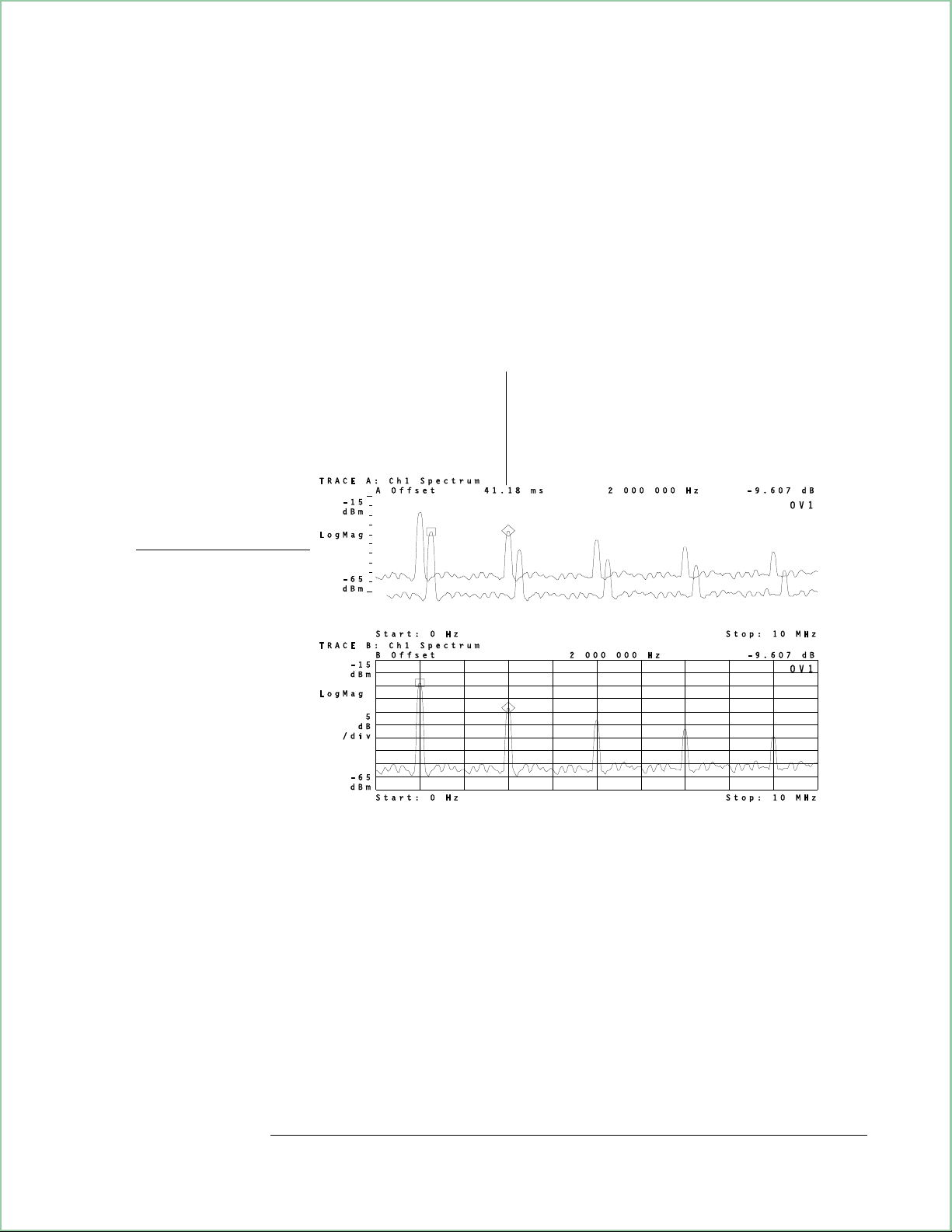
Using Waterfall and Spectrogram Displays (Opt. AYB)

6. Move the marker to the next trace in the waterfall display.

Press [Marker Function] followed by the up-arrow key.

In this example, notice that the z-axis marker value is approximately 41.2 ms, which is the elapsed time between the two traces. In other words,

41.2 ms elapsed from when the analyzer acquired trace 2 to when it acquired trace 1. The amount of time needed to acquire each trace is dependent on several factors and may be different than that shown in this example.

When the offset marker is on, marker values are relative to the offset marker. In this example, the selected trace was acquired approximately

41.2 ms after the previous trace.

A diamond shows the location of the marker. A square shows the location of the offset marker.

Using Markers with a Waterfall Display

7 - 9

Using Waterfall and Spectrogram Displays (Opt. AYB)

To use buffer search in waterfall displays

This procedure shows you how to use buffer search to do marker-search operations over all traces in the waterfall buffer. Start with step 2 if you just finished the previous procedure.

1. If you just finished the previous procedure, skip this step.

Otherwise, configure the analyzer for this procedure by following the instructions in “To select a trace in a waterfall display.”

2. Turn buffer search on.

Press [Marker Search][buffer search on].

With buffer search on, marker-search operations include all traces in the waterfall buffer. With buffer search off, marker-search operations are confined to the selected trace.

Some marker-search operations are unavailable when buffer search is on. The softkeys for these operations are ghosted to inform you that the operations are unavailable.

3. Move the marker to the highest peak in the waterfall buffer.

Press [marker to peak]

Press [Shift][Marker].

[Shift][Marker] is a shifted function, as indicated by the blue label above the [Marker] hardkey, that duplicates the [marker to peak] operation.

4. Move the marker to the next highest peak in the waterfall buffer.

Press [Marker Search][next peak].

Notice that the marker moved to the next highest peak in the waterfall buffer which, in this example, is on a different trace.

5. Move the marker to the lowest point in the waterfall buffer.

Press [Marker Search][marker to minimum].

7 - 10

Using Waterfall and Spectrogram Displays (Opt. AYB)

To set up a spectrogram display

This procedure shows you how to set up and view a spectrogram display.

1. Perform the procedure at the beginning of this chapter to create a test signal.

2. Turn on the spectrogram display for trace A.

Press [A] to activate trace A. Press [Display][spectrogram setup][spectrogram on].

3. Set the size of the trace buffer.

Press [buffer depth]50[enter].

Press [Meas Restart] to start a new spectrogram measurement.

Notice that you set up a spectrogram display in much the same way as a waterfall display. Both displays share the same trace buffer. Therefore, you may switch between waterfall and spectrogram displays without losing data.

A spectrogram display is simply another method of looking at trace data. In a spectrogram, the y-axis is reduced to a single line, where color represents different y-axis values. Therefore, each trace occupies a single, horizontal line on the display. Because of this, a single-grid spectrogram display requires about 300 traces to fill the entire display.

A spectrogram uses a colorbar to represent the y-axis. The colorbar shows how colors are distributed along the y-axis and the y-axis value of each color.

The flow of trace data in a spectrogram display is opposite a waterfall display. In a waterfall display, traces flow from the top to the bottom of the display, with the most recent trace at the top. In a spectrogram display, traces flow from the bottom to the top of the display, with the most recent trace at the bottom.

For additional information, see online help for the [spectrogram setup] softkey.

7 - 11

Using Waterfall and Spectrogram Displays (Opt. AYB)

To enhance spectrogram displays

This procedure shows you how to use advanced features to enhance the spectrogram display.

1. Perform the previous procedure, “To set up a spectrogram display.”

2. Pause the measurement after the spectrogram fills the entire display.

Press [Pause|Single].

3. Adjust the mapping of amplitude to color to obtain the best display.

Press [ Press [enhance] and rotate the knob to obtain the best spectrogram display.

The [enhance] softkey lets you redistribute colors in the colorbar. A value of 50% evenly distributes the colors. A value of 0% compresses the colors into the top of the colorbar, whereas a value of 100% compresses them into the bottom of the colorbar. Online help provides additional information on this feature.

Marker|Entry

] to illuminate the Entry LED.

4. Select different color maps to see the effects on the spectrogram display.

Rotate the knob to until [enhance] is back to its default value of 50%. Press [map color][color reverse] Press [grey normal] Press [grey reverse] Press [color normal] to return to the default color map.

Color maps change the colors used in the color bar. Different color maps offer different perspectives. Essential information may be buried, or obscure in one color map, but prominent in another.

7 - 12

Using Waterfall and Spectrogram Displays (Opt. AYB)

5. Change the number of colors used in the color map.

Press [return]. Press [ Press 5 [enter]. Press 10 [enter]. Press 64 [enter] to return to the default number of colors.

In this example, changing the number of colors erases the upper portion of the spectrogram display. This happens because the traces in this area are not in the spectrogram buffer. In other words, the spectrogram buffer does not contain enough traces to fill the entire display. Changing the number of colors forces the analyzer to recompute scaling factors for the y-axis. The analyzer can do this only for traces in the spectrogram buffer.

number colors

] 2 [enter].

6. Adjust the threshold to remove noise from the spectrogram display.

Press [threshold]. Rotate the knob to obtain the desired display.

As demonstrated, you can use the threshold feature to hide unwanted information. When you specify a threshold, the analyzer displays colors at or above the threshold; below the threshold, the analyzer uses the bottom color in the colorbar.

You specify threshold as a percentage of the colorbar. A threshold of 0% displays the entire signal. A threshold of 50% only displays colors in the upper half of the colorbar—colors below this point (or threshold) are displayed in the same color as the bottom color in the colorbar.

Hint You may overlay another type of trace on a spectrogram and observe, for

example, the spectrum or PSD of the input signal. To do this, press [Display] [view/overlay traces] and turn on the trace that you want to use as an overlay.

Color map, enhance, and threshold affect all traces that contain spectrogram displays. For example, if traces A and B contain spectrogram displays, changing the color map for trace A also affects trace B.

7 - 13

Using Waterfall and Spectrogram Displays (Opt. AYB)

To use markers with spectrogram displays

You use markers in a spectrogram display the same way you use markers in a waterfall display. To learn how to use markers (and select traces) in a spectrogram display, display a spectrogram instead of a waterfall and perform the following procedures:

To select a trace in a waterfall display.

To use markers with waterfall displays.

To use buffer search in waterfall displays.

Note the following differences when performing the above procedures with a spectrogram dispay.

Spectrograms use a vertical line instead of a diamond to show the location of

the marker.

Spectrograms use a vertical line and a horizontal line with a square to show the

location of the offset marker.

Spectrograms use a horizontal line to show the selected trace when trace select

is on.

7 - 14

Using Waterfall and Spectrogram Displays (Opt. AYB)

To save waterfall and spectrogram displays

You save a waterfall or spectrogram display by saving the trace buffer. The trace buffer contains the traces that make up the waterfall or spectrogram display. Both waterfall and spectrogram displays share the same trace buffer (which is why you can switch between waterfall or spectrogram displays without losing data).

1. Select the desired depth for the trace buffer:

Press [ OR Pr ess [

2. Activate the waterfall or spectrogram display that you want to save. For

example, if the display is in trace A, press [A].

3. Save the trace buffer in a file or data register:

Press [

][

Display

Save/Recall

waterfall setup

][spectrogram setup][

], [

save more

][

buffer depth

], [

save trace buffer

buffer depth

Waterfall and spectrogram displays share the same trace buffer. Therefore, it doesn’t matter which is displayed when you save the trace buffer. When you recall the trace buffer, you can examine trace-buffer data in either waterfall or spectrogram format.

The size of the trace buffer determines the number of traces that are saved. For example, a buffer depth (trace buffer size) of 10 means ten traces will be saved, regardless of how many traces are displayed. Save the trace buffer to a file if you want to recall the trace buffer after a power down.

Memory constraints may affect trace-buffer size. For details, see online help for the [

remove trace buffers

] softkey (under [

System Utilities

][memory usage]).

7 - 15

Using Waterfall and Spectrogram Displays (Opt. AYB)

To recall waterfall and spectrogram displays

This procedure shows you how to recall waterfall and spectrogram displays. See the previous procedure for instructions on saving waterfall and spectrogram displays.

1. Activate the trace where you want the waterfall or spectrogram display. For

example, if you want to display a waterfall display in trace A, press [A].

2. Turn on the waterfall or spectrogram display.

Press [ OR Press [

Display

3. If the trace buffer is in a file, recall the trace buffer from the file into a data

Cho ose a file and data register.

][

Display

Save/Recall

waterfall setup

][spectrogram setup][

], [

recall more

][

waterfall on

spectrogram on].

], [

recall trace buffer

4. Display the data register:

Press [ Choose the desired data register.

Any trace buffer may be recalled as either a spectrogram or a waterfall, regardless of which display was selected at the time the buffer was stored. If the data register contains only one trace, then the waterfall or spectrogram only displays the single scan.

Measurement Data

], [

data reg

]

7 - 16

Using Digital Demodulation (Opt. AYA)

This chapter shows you how to use digital demodulation to demodulate and view digitally modulated signals. You may perform the tasks in this chapter using signals from the Signals Disk, or you may use these tasks as a model for demodulating your own signals.

8 - 1

Using Digital Demodulation (Opt. AYA)

To prepare a digital demodulation measurement

This task shows you one way to set up a digital demodulation measurement. The task uses a NADC signal from the signals disk. Several other tasks in this chapter use this setup to teach you how to use digital demodulation.

1. Initialize the analyzer:

Press [

89410A: [

89441A: [ Press [ Press [

Instrument Mode

input section (0-10 MHz) RF section (0-10 MHz)

Preset

Instrument Mode

], [

2. Supply a NADC signal to the channel 1 INPUT or perform the following steps to

load a NADC signal from the Signals Disk into a data register and play it through the analyzer’s aribtrary source:

Insert the Signals Disk into the internal disk drive. Connect the SOURCE to the channel 1 INPUT. Press [ Press [

Save/Recall

Return

Rot ate the knob to highlight PI4DQPSK.DAT Press [ Press [

recall trace

Source

], [

default disk

], [

catalog on].

], [

from file into D1

], [

source on], [source type

], then press:

receiver

vector

], [

internal disk

], [

enter

], [

arbitrary

3. Select the optimum range:

Press [ Press the down-arrow key until the Channel-1 Over and Half LEDs are on. Press the up arrow key one press at a time until the Over LED turns off.

For additional details about selecting the optimum range, see online help for the [

Range

Range], [ch1 range] softkey.

4. Select a center frequency and span:

Press [ Press [

Frequency

span

The center frequency tunes the analyzer to the carrier frequency. To obtain reliable carrier lock, the center frequency must be close to the carrier frequency. For details, see ‘’Carrier Locking’’ in the Digital Demodulation Concepts (Opt. AYA) chapter.

Selecting the correct frequency span is also important when using digital demodulation. The span must be wide enough to include all signal components, and yet not too wide, or the measurement may be affected by excessive noise and slower speed. For details, see ‘’Span considerations for digitally demodulationed measurements’’ in the Digital Demodulation Concepts (Opt. AYA) chapter.

], [

], 100, [

center

kHz

], 5, [

MHz

]

8 - 2

Using Digital Demodulation (Opt. AYA)

5. Set up the trigger:

Press [

This example uses a signal which has been supplied from the Signals Disk. When you supply another signal to the channel 1 input you need to select appropriate center frequency, span, range, and triggering parameters prior to demodulating the signal.

Trigger

], [

trigger type

], [

internal source

], [

return

], [

ch1 delay

], 1, [ms].

The spectrum of a digitally modulated carrier before demodulation.

8 - 3

Using Digital Demodulation (Opt. AYA)

To demodulate a standard-format signal

This task shows you how to demodulate the NADC signal on the Signals Disk.

1. Configure the analyzer for a digital demodulation measurement.

If you haven’t already done so, perform the steps in the previous task, ‘’To prepare a digital demodulation measurement.’’

2. Digitally demodulate the signal:

Press [ [

Instrument Mode

], [

demod type

Digital Demodulation

], [

Digital Demodulation

3. Choose standard demodulation setup parameters:

Press [

demodulation setup

], [

demod format

4. Modify the standard parameters for this specific signal:

Press [ Press [

Press

], [

Time pulse search off]

[Auto Scale

result length

]

], 100, [

] (with option AYH, press

], [

Return].)

], [

standard setups

]

sym

], [

NADC

If you are demodulating a signal which matches a standard signal type, you can automatically configure the analyzer for that standard by pressing

standard setups] and then choosing the appropriate type. The parameters set

[ when you choose a standard are: demod format, span, symbol rate, meas filter, ref filter, alpha/BT, result length, pulse search, and points per symbol. If your signal is not of a standard type you may select individual parameters in the [

demodulation setup] menu. To learn how to do this, see ‘’To

demodulate a non-standard-format signal’’ in the Analyzing Digitally Demodulated Signals chapter.

A time display of a demodulated signal

8 - 4

Using Digital Demodulation (Opt. AYA)

To select measurement and display features

The analyzer provides many different ways of viewing demodulated data. This task shows you how to display demodulated data two different views in two grids.

1. Demodulate your signal as shown in the previous task.

2. Select multiple display grids:

Press [

3. Change the measurement data for trace B:

Press [

4. Change the data format for trace A:

Press [

], [

Display

], [

Measurement Data

], [

Data Format

4 grids quad

], [

error vector spectrum

polar IQ constell ation

]

The [ to see, while the [ data. You may select different measurement data and data formats for up to four traces by activating each trace individually.

Measurement Data

] menu allows you to select the type of data you want

Data Format

] menu selects how you want to display that

Each grid shows a different measurement type with an appropriate data format.

8 - 5

Using Digital Demodulation (Opt. AYA)

To set up pulse search

In this example you learn how to perform pulse search on a burst signal. This example uses a signal, provided on the Signals Disk, which is a record of the output of a keyed NADC radio transmission.

1. Load “MEAS_PI4.DAT” from the Signals Disk into the arbitrary source:

Perform steps 1, 2, and 3 in ‘’To prepare a digital demodulation measurement.’’ For step 2, load the “MEAS_PI4.DAT” signal from the Signals Disk instead of ‘’PI4DQPSK.DAT.’’

2. Select appropriate setup parameters:

Press [ Press [ Press [ Press [

If you don’t know how to select the optimum range, see ‘’To prepare a digital demodulation measurement.’’

Range] and select the optimum range. Frequency

], 100, [

span

Trigger

], [

], 5, [

center

kHz

trigger type

], [

internal source

MHz

]

], [

return

], [

ch1 delay

], 1, [ms].

3. Select appropriate demodulation parameters:

Press [ [

Instrument Mode

Press

Instrument Mode

[demodulation setup

], [

demod type

], [

Digital Demodulation

], [

demod format

Digital Demodulation

] (with option AYH, press

], [

Return].)

], [

standard setups

], [

NADC

4. Select pulse and result lengths for this particular signal:

Press [ Press [

], [

Time

result length

search length

], 156, [

], 500, [

sym

]

5. Select measurement, display, and analysis features. For example, to view the

default displays for all four traces: Press [

Display

], [

4 grids quad

]

6. The search length must be longer than result length and must include at least

one entire pulse. If the search length is long enough to include more than one pulse, only the first pulse is demodulated. For additional details, see the Digital Demodulation Concepts (Opt. AYA) chapter and see online help for

pulse search] and [search length] softkeys.

the [

8 - 6

Demodulating a pulsed signal

Using Digital Demodulation (Opt. AYA)

8 - 7

Using Digital Demodulation (Opt. AYA)

To set up sync search

In this task you learn how to synchronize your measurement by using a specific bit pattern within the chain of bits. You learn how to define sync words and set an offset. Since sync search is often used with pulsed signals, this example assumes you have already acquired and demodulated a pulsed signal as shown in the previous task.

1. Select two displays and format them:

Press [ Press [ Press [ Press [

2. Enter a sync bit pattern:

Press [

3. Select an offset:

Press [

4. Turn on sync search:

Press [

], [

Display

], [

Measurement Data

Data Format

], [

Time

offset

Return

sync setup

], 6, [

], [

]

2 grids

], [magnitude

], [

sym

sync search on

], [

IQ measured time

log(dB)

], [

pattern

]

clear entry

], 000101, [

enter

The search length must be longer than the combination of result length, sync pattern, and offset. The sync pattern may include up to 32 symbols. The offset may be positive or negative. See the online help topics for more information on these keys.

The sync word is highlighted when sync search is completed successfully

8 - 8

Using Digital Demodulation (Opt. AYA)

To select and create stored sync patterns

When using sync search you can enter a sync bit pattern as in the previous task, or you can load up to six of your own sync patterns into softkeys F3 through F8 and then use the softkeys to select a sync bit pattern. This task assumes you have completed the previous task.

1. Insert the Signals Disk into the analyzer’s disk drive.

2. Load an example of user-defined sync patterns:

Press [ Scroll to highlight SYNC_KEY.TXT Press [

Save/Recall

recall more

], [

catalog on

], [

recall sync/state defs

3. Choose one of the user-defined sync patterns:

Press [ Pres s one of the six user-defined softkeys to change sync patterns.

If you select Sync 1, Sync 5, or Sync 6 you see what happens if the analyzer cannot find the sync pattern. The analyzer demodulates the signal but displays the message “SYNC NOT FOUND.” When this happens the result is positioned at the start of data collection. In this case the sync is not found because the combination of offset and sync word place the result length beyond the pulse. The other four sync words show the result length on the leading edge, trailing edge, or center of the pulse.

Time

], [

sync setup

], [

offset

], [

enter

], 15, [

sym

], [

user sync patterns

You can create your own sync bit pattern definitions for the softkeys. See the file “STAT_DEF” on the Signals Disk. The file may be viewed and edited with any ASCII editor and the results may be saved to disk. If you have IBASIC installed, you may use it as an editor. See “SYNC_KEY.TXT” and “STATES.TXT” files to see a sync pattern and state definition that were created using IBASIC to modify portions of the “STAT_DEF” file.

Up to 6 sync patterns may be loaded into softkeys to facilitate changing sync patterns.

8 - 9

Using Digital Demodulation (Opt. AYA)

To demodulate and analyze an EDGE signal

This task shows you how to demodulate an EDGE (Enhanced Data rates for GSM Evolution) signal. The EDGE signal used in this task was generated with the HP/Agilent E4433 ESG Series Signal Generator, with a frequency of 5 MHz, amplitude of 0 dBm, and a framed (pulsed) data format. Option B7A must be installed to demodulate EDGE signals.

1. Initialize the analyzer:

Press [

89410A: [

89441A: [ Press [

Instrument Mode

input section (0-10 MHz) RF section (0-10 MHz)

Preset

], [

2. Connect your EDGE signal to the channel 1 INPUT.

3. Set the center frequency (this example uses a 5 MHz EDGE signal):

Press [

Frequency

], [

center

4. Select the optimum range:

Press [ Press the down-arrow key until the Channel-1 Over and Half LEDs are on. Press the up arrow key one press at a time until the Over LED turns off.

Range

], then press:

receiver

], 5, [

MHz

]

For additional details about selecting the optimum range, see online help for the [

Range], [ch1 range] softkey.

5. Turn on digital demodulation:

Press [ [

Instrument Mode

], [

demod type

], [

Digital Demodulation

], [

Digital Demodulation

] (with option AYH, press

], [

Return].)

6. Configure the analyzer to demodulate the EDGE signal:

Press [

demodulation setup

], [

demod format

], [

standard setups

], [EDGE].

7. Display four grids to view the vector diagram (trace A), error-vector trace

(trace B), eye diagram (trace C), and symbol table (trace D). Press

[Display

], [

4 grids quad

8. Autoscale traces A, B, and C:

Press Press

[Shift] [

[Auto Scale].

], [

Shift][C

]

8 - 10

Using Digital Demodulation (Opt. AYA)

9. Display the ideal vector diagram in trace C and compare it to trace A:

Press [ Press [ Press [ Press

Selecting the EDGE standard setup automatically sets the demodulation format, frequency span, symbol rate, filtering, and several other demodulation parameters (for a complete list, see help for [

Because EDGE signals incorporate rotation and the EDGE filter introduces ISI (inter-symbol interference), symbol locations in the vector and constellation diagrams should appear random. However, at one point/symbol (the value set by the EDGE standard setup) the analyzer removes the effects of ISI so you can view a “clean” vector diagram. Above one point/symbol, the analyzer does not remove the effects of ISI.

], [

Measurement Data

Data Format

more format setup

[Shift][A

], [

], [Auto Scale].

], [

IQ reference

polar IQ vector

], [

symbol dots

]

time

]

standard setups

10. Set points/symbol to 2 to view the effects of ISI on the vector diagram:

Press [ Press [

A], [Display Time

], [

points/symbol

], [

single grid

], 2,[

]

enter

]).

Quad display showing individual IQ measured and IQ reference vector diagrams, the error vector trace, and the symbol table (at 1 point/symbol). Single display showing same vector diagram, but at 2 points per symbol. At 1 point/symbol, the analyzer removes the effects of ISI so you can view a “clean” vector diagram. Above 1 point/symbol, the effects of ISI are not removed.

8 - 11

Using Digital Demodulation (Opt. AYA)

To troubleshoot an EDGE signal

This task shows you how to use the error-vector trace and the symbol table to diagnose problems with an EDGE signal. To simulate an error condition, the task uses the analyzer’s source to mix a 5.1 MHz, –35 dbM sine wave with the EDGE signal loaded in the previous task.

1. Demodulate your EDGE signal as shown in the previous task.

2. Make sure points/symbol are set to one:

Press [

Time

], [

points/symbol

3. Mix the analyzer’s source with your EDGE signal.

Connect a T-connector to the CHANNEL 1 input. Connect the analyzer’s SOURCE output to the T-connector. Connect your EDGE signal to the T-connector.

4. Configure the source to output a 5.01 MHz, –35 dbM, sine wave:

Press [ Press [ Press [ Press [

]

Source

], [

level sine freq source on]

–35

], [

5.01

dbM

], [

], 1,[

]

MHz

enter

5. Display the error-vector in trace A and autoscale the trace:

Press [ Press [ Press [

], [

Measurement Data Data Format Auto Scale

], [

polar IQ vector

], [

error vector time

]

6. Display two grids and put the symbol table in the lower trace.

Press [ Press [

The error-vector vector diagram and symbol table provide good insight into the quality of your EDGE signal. The next step shows you another useful display: the error-vector spectrum.

], [

Display

] (By default, the symbol table is in trace D).

two grids

7. Display the spectrum of the error-vector in trace A and auto-scale the trace.

Press [ Press

You use the same methods to troubleshoot an EDGE signal as you do other types of digital signals. For example, you still use error parameters in the symbol table to help you determine the quality of an EDGE signal. The symbol table reports error parameters such as Mag Err (Magnitude Error), Phase Err (Phase Error), Freq Err (Frequency Error), EVM (Error Vector Magnitude), and SNR (Signal-to-Noise Ratio).

], [

Measurement Data

[Auto Scale

], [

Ierror vector spectrum

]

8 - 12

Agilent 89441A Operating Guide

Specifications and Main Features

Frequently Asked Questions

User Manual

The Analyzer at a Glance

Notation Conventions

TABLE OF CONTENTS