

Page 1

Quick Reference Guide
HP
8753E Network Analyzer
HEWLETT
FB
HP Part No. 08753-90368 Supersedes January 1998
Printed in USA October 1998
PACKARD
Page 2

Notice.
The information contained in this document is subject to change without
notice.
Hewlett-Packard makes no warranty of any kind with regard to
this material, including but not limited to, the implied warranties of
merchantability and fitness for a particular purpose.
Hewlett-Packard
shall not be liable for errors contained herein or for incidental or
consequential damages in connection with the furnishing, performance,
or use of this material.
@Copyright 1998 Hewlett-Packard Company
Page 3

Regulatory Information
The regulatory information is in the User’s Guide supplied with the
analyzer.
Safety, Warranty, and Assistance
Refer to the User’s Guide for information on safety, warranty, and
assistance.
iii
Page 4

HP 87533 Network Analyzer
Documentation Map
The Installation and Quick Start Guide
familiarizes you with the
HP 8763E/Option 011 network analyzer’s
front and rear panels, electrical and
environmental operating requirements, as
well
as procedures for installing, configuring,
and verifying the operation of the analyzer.
The User’s Guide shows how to make
measurements, explains commonly-used
features, and tells you how to get the most
performance from your analyzer.
The Quick Reference Guide provides a
summary of selected user features.
a
@
The
HP-II3
Programming and Command
BP-B3
0
I!3
Reference Guide provides programming
information for operation of the network
analyzer under
control.
iv
The HP BASIC Programming Examples
Guide provides a tutorial introduction using
BASIC programming examples to
demonstrate the remote operation of the
network analyzer.
The System Verification and Test Guide
provides the system verification and
performance tests and the Performance Test
Record for your HP 8763E/Option 011
network analyzer.
Page 5

Contents
1.
HP 87533 Front and Rear Panel
Front Panel Features
Analyzer Display
Rear Panel Features and Connectors
2. Making Measurements
Basic Measurement Sequence and Example
Basic Measurement Sequence
Basic Measurement Example
Step 1. Connect the device under test and any required
test equipment.
Step 2. Choose the measurement parameters.
Step 3. Perform and apply the appropriate
error-correction.
Step 4. Measure the device under test.
Step 5. Output the measurement results.
Using the Display Functions
‘lb View Four Channels Simultaneously
Description of the Auxiliary Channels
Quick Four-Parameter Display
‘lb Make an Auxiliary Channel Active:
lb Save a DataTrace to the Display Memory
lb View the Measurement Data and Memory Trace
lb Divide Measurement Data by the Memory Trace
‘lb Subtract the Memory Trace from the Measurement
Data Trace
‘RI
Ratio Measurements in Channel 1 and 2
lb Title the Active Channel Display
Using Markers
‘lb Activate Display Markers
Delta Markers and Statistics
Search for a Specific Amplitude
Searching for the Maximum Amplitude
Searching for the Minimum Amplitude
Markers and the Backspace Key
..................
...................
.............
.............
................
................
..............
...................
.....................
.............
.............
..........
.......
....
.......
......
........
........
............
........
.....
. .
. .
......
..........
............
.......
.......
...........
l-l
l-4
l-9
2-2
2-2
2-2
2-2
2-2
2-3
2-3
2-3
2-4
2-4
2-5
2-6
2-6
2-7
2-7
2-8
2-8
2-8
2-8
2-9
2-9
2-9
2-10
2-10
2-10
2-11
Contents-l
Page 6

‘lb Move Marker Information off of the Graticules
‘Ib
Move Marker Information back onto the Graticules
Testing A Device with Limit Lines
Creating Flat Limit Lines
...............
Creating a Sloping Limit Line
Creating Single Point Limits
Editing Limit Segments
................
Deleting Limit Segments
RunningaLimitTest
.................
Reviewing the Limit Line Segments
Activating the Limit
Test
Measuring Gain Compression
Measurements using the Swept List Mode
Connect the Device Under Test
Observe the Characteristics of the Filter
Choose the Measurement Parameters
Set Up the Lower Stop Band Parameters
SetUptheBassBandParameters
Set Up the Upper Stop Band Parameters
Calibrate and Measure
................
...........
.............
.............
..............
.........
..............
..............
........
............
.......
.........
......
..........
......
. .
2-11
2-12
2-13
2-13
2-16
2-18
2-20
2-20
2-21
2-21
2-21
2-22
2-27
2-28
2-29
2-30
2-30
2-30
2-31
2-31
3. Making
Mixer
Measurements
Measurement Considerations . . . . . . . . . . . . . .
Minimizing Source and Load Mismatches . . . . . . .
Reducing the Effect of Spurious Responses . . . . . .
Eliminating Unwanted Mixing and Leakage Signals . . .
HowRFandIFAreDefined . . . . . . . . . . . . .
Frequency Offset Mode Operation . . . . . . . . . . .
Differences Between Internal and External R Channel
Inputs . . . . . . . . . . . . . . . . . . . . . .
Power Meter Calibration . . . . . . . . . . . . . . .
Conversion Loss using the Frequency Offset Mode . . . .
High Dynamic Range Swept RF/IF Conversion Loss
Conversion Compression using the Frequency Offset Mode
Isolation Example Measurements . . . . . . . . . . . .
LO to IF Isolation . . . . . . . . . . . . . . . . . .
RF Feedthrough . . . . . . . . . . . . . . . . . . .
Contents-Z
. . .
3-l
3-l
3-2
3-2
3-2
3-4
3-4
3-5
3-6
3-12
3-16
3-2 1
3-22
3-23
Page 7

4. Printing, Plotting, and Saving Measurement Results
ConIlguring
Defining a Print Function
If You Are Using a Color Printer
lb Reset the Printing Parameters to Default Values
ConIlguring
If You Are Plotting to an
If You Are Plotting to a Pen Plotter
If You Are Plotting to a Disk Drive
Defining a Plot Function
Choosing Display Elements
Selecting Auto-Feed
Selecting Pen Numbers and Colors
Selecting Line Types
Choosing Scale
Choosing Plot Speed
‘lb Reset the Plotting Parameters to Default Values
If You Are Plotting to an HPGL Compatible Printer
‘Ib
Save Measurement Results
Recalling an Instrument State
a Print Function
..............
...............
...........
a Plot Function
..............
HPGL/2
Compatible Printer .
..........
..........
................
..............
.................
..........
.................
....................
.................
..............
.............
...
...
. .
5. Optimizing Measurement Results
Increasing Measurement Accuracy
Connector Repeatability
Interconnecting Cables
Temperature Drift
Frequency Drift
...................
Performance Verification
...............
................
..................
...............
Reference Plane and Port Extensions
Measurement Error-Correction
Clarifying Type-N Connector Sex
...........
.........
.............
...........
Response Error-Correction for Reflection Measurements
Response Error-Correction for Transmission
Measurements
..................
Response and Isolation Error-Correction for Transmission
Measurements
One-Port Reflection Error-Correction
Full Two-Port Error-Correction
Power Meter Measurement Calibration
Entering the Power Sensor Calibration Data
Compensating for Directional Coupler Response
Using Sample-and-Sweep Correction Mode
Using Continuous Correction Mode
Increasing Sweep Speed
lb Use Swept List Mode
..................
..........
.............
.........
......
....
.......
..........
................
...............
4-l
4-2
4-2
4-2
4-3
.
4-3
4-4
4-5
4-6
4-6
4-6
4-7
4-8
4-9
4-9
4-9
4-9
4-10
4-12
5-l
5-l
5-l
5-l
5-2
5-2
5-2
5-3
5-3
5-3
5-4
5-4
5-6
5-7
5-9
5-9
5-9
5-10
5-l
1
5-12
5-12
Contents-3
Page 8

‘Ib Decrease the Frequency Span
lb Set the Auto Sweep Time Mode
‘lb
Widen the System Bandwidth
‘Ib Reduce the Averaging Factor
...........
..........
...........
...........
lb Reduce the Number of Measurement Points
'IbSettheSweepType
lb Activate Chop Sweep Mode
lb Use Fast
2-Port
Increasing Dynamic Range
Increase the
Test Port
Reduce the Receiver Noise Floor
Change System Bandwidth
Change Measurement Averaging
Reducing Trace Noise
Activate Averaging
Change System Bandwidth
Reducing Receiver Crosstalk
................
............
Calibration
............
...............
Input Rower
..........
...........
.............
..........
.................
..................
..............
..............
6. Softkey Locations
7. Error Messages
Error Messages in Alphabetical Order . . . . . . . . . .
Index
.....
5-13
5-13
5-14
5-14
5-15
5-15
5-16
5-16
5-17
5-17
5-17
5-17
5-17
5-18
5-18
5-18
5-18
7-l
Contents-4
Page 9

Figures
l-l. BP 87533 Front Panel
l-2.
Analyzer Display (Single Channel, Cartesian Format) . .
l-3. BP 87533 Rear Panel
2-l.
Basic Measurement Setup
2-2. Four Parameter Display
2-3. Marker 1 as the Reference Marker
2-4. Example Statistics of Measurement Data
2-5. Markers before Pressing the Backspace Key
2-6. Markers after Pressing the Backspace Key
2-7. Example Flat Limit Line
2.8. Example Flat Limit Lines
2-9. Sloping Limit Lines
2-10. Example Single Point Limit Lines
2-11. Diagram of Gain Compression
2-12. Gain Compression using Linear Sweep and
DZ:,Dl
2-13. Gain Compression using Power Sweep
2-14. Swept List Measurement Setup
2-15. Characteristics of a Filter
2-16. Calibrated Swept List Thru Measurement
2-17. Filter Measurement using Linear Sweep
(Power: 0
2-18. Filter Measurement using Swept List Mode
3-l.
Down Converter
3-2. Up Converter
3-3. An Example Spectrum of RF, LO, and IF Signals Present
in a Conversion Loss Measurement
3-4. Connections for R Channel and Source Calibration
3-5. Connections for a One-Sweep Power Meter Calibration for
Mixer Measurements
3-6. Measurement Setup from Display
3-7. Conversion Loss Example Measurement
3-S.
Connections for Broad Band
3-9. Connections for Receiver Calibration
t.0 DZ OH
dBm/lF
Port
................
................
..............
...............
..........
.......
......
.......
...............
...............
.................
...........
............
..............
.........
............
..............
.......
BW: 3700
Port
Connections
Connections
Hz)
.........
......
..........
............
........
...............
...........
........
Power
Meter Calibration
.........
...
2-10
2-l
2-12
2-14
2-15
2-17
2-19
2-22
2-24
2-26
2-28
2-29
2-32
2-33
2-34
3-10
3-11
3-13
.
3-13
l-l
l-4
l-9
2-2
2-5
2-9
1
3-3
3-3
3-6
3-7
3-9
Contents-5
Page 10

3-10. Connections for a High Dynamic Range Swept IF
Conversion Loss Measurement . . . . . . . . . .
3-11. Example of Swept IF Conversion Loss Measurement . .
3-14
3-15
3-12. Conversion Loss and Output Power as a Function of Input
Power Level Example . . . . . . . . . . . . . .
3-16
3-13. Connections for the First Portion of Conversion
Compression Measurement . . . . . . . . . . . .
3-17
3-14. Connections for the Second Portion of Conversion
Compression Measurement . . . . . . . . . . . .
3-15. Measurement Setup Diagram Shown on Analyzer Display
3-18
3-19
3-16. Example Swept Power Conversion Compression
Measurement . . . . . . . . . . . . . . . . . .
3-17. Signal Flow in a Mixer Example
. . . . . . . . . . .
3-18. Connections for a Mixer Isolation Measurement . . . .
3-19. Example Mixer LO to RF Isolation Measurement . . . .
3-20. Connections for a Mixer RF Feedthrough Measurement .
3-21. Example Mixer RF Feedthrough Measurement . . . . .
4-l. Plot Components Available through Definition . . . . .
4-2. Line Types Available . . . . . . . . . . . . . . . . .
4-3. Locations of Pl and P2 in :XHLE
PLOT C GHHTI
Mode . . . . . . . . . . . . . . . . . . . . . .
4-4. Data Processing Flow Diagram . . . . . . . . . . . .
5-l.
Standard Connections for a Response Error-Correction for
Reflection Measurement . . . . . . . . . . . . .
3-20
3-21
3-22
3-22
3-23
3-23
4-6
4-8
4-9
4-11
5-3
5-2. Standard Connections for Response Error-Correction for
Transmission Measurements . . . . . . . . . . .
5-4
5-3. Standard Connections for a Response and Isolation
Error-Correction for Transmission Measurements . .
5-5
5-4. Standard Connections for a One-Port Reflection
Error-Correction . . . . . . . . . . . . . . . . .
5-5. Standard Connections for
Full
Two-Port Error-Correction
5-6. Sample-and-Sweep Mode for Power Meter Calibration
5-7. Continuous Correction Mode for Power Meter Calibration
5-6
5-7
.
5-10
5-11
Contents-f3
Page 11

‘Ihbles
2-l.
Connector Care Quick Reference
4-l.
Default Pen Numbers and Corresponding Colors
4-2. Default Pen Numbers for Plot Elements
4-3. Default Line Types for Plot Elements
5-l.
Band Switch Points
6-1.
Softkey
Locations
.................
..................
...........
....
........
.........
2-l
4-7
4-7
4-a
5-13
6-2
Contents-7
Page 12

1
HP 87533 Front and Rear Panel
Front Panel Features
Caution
Figure l-l shows the location of the following front panel features and
key function blocks. These features are described in more detail later in
this chapter.
Do not mistake the line switch for the disk eject
button. See the figure below. If the line switch is
mistakenly pushed, the instrument will be turned off,
losing all settings and data that have not been saved.
Figure l-l. HP 87533 Front Panel
LINE switch.
1.
on, 0 is off.
This switch controls ac power to the analyzer. 1 is
HP 87533 Front and Rear Panel
l-l
Page 13

2.
Display.
This shows the measurement data traces, measurement
annotation, and softkey labels. The display is divided into specific
information areas, illustrated in Figure
l-2.
3.
Disk drive.
This 3.5 inch drive allows you to store and
recall
instrument states and measurement results for later analysis.
Disk eject button.
4.
5.
Softkeys.
These keys provide access to menus that are shown on
the display.
6.
STlMULUS
function block. The keys in this block allow you to
control the analyzer source’s frequency, power, and other stimulus
functions.
RJZSPONSE
7.
function block. The keys in this block allow you
to control the measurement and display functions of the active
display channel.
ACTIVE CHANNEL keys.
8.
These keys activate one of the four
measurement channels. Once activated, a channel can then be
configured for making measurements.
The analyzer has four display channels.
1 or 3, and
(Chanj
activates channel 2 or 4. Refer to “Using
(-1)
activates channel
Display Functions” in Chapter 2 for information on enabling
channels 3 and 4 and making them active.
The ENTRY block.
9.
This block includes the knob, the step @)
keys, and the number pad. These allow you to enter numerical
data and control the markers.
You can use the numeric keypad to select digits, decimal points,
and a minus sign for numerical entries. You must also select a units
terminator to complete value inputs.
The backspace key @ has two independent functions:
@
H
Modifies entries and test sequences.
n
Turns off the
softkey
menu and, if more than one marker is
active, the marker information is displayed in the softkey area.
Refer to “Markers and the Backspace Key” in Chapter 2.
1-2
HP 87533 Front and Rear Panel
Page 14

10. INSTRUMENT STATE function block. These keys allow you
to control channel-independent system functions such as the
following:
w
copying, save/recall, and
w
limit testing
n
external source mode
n
tuned receiver mode
n
frequency offset mode
n
test sequence function
n
harmonic measurements (Option 002)
n
time domain transform (Option 010)
HP-R3
STATUS indicators are also included in this block.
11.
IPreseT) key.
This key returns the instrument to either a known
factory preset state, or a user preset state that can be
HP-R3
controller mode
deEned.
Refer to the “Preset State and Memory Allocation” chapter for a
complete listing of the instrument preset condition.
12.
PROBE POWER connector.
This connector (fused inside the
instrument) supplies power to an active probe for in-circuit
measurements of ac circuits.
13.R CX4NNEL connectors.
These connectors allow you to apply an
input signal to the analyzer’s R channel, for frequency offset mode.
14.
PORT 1 and PORT
2. These ports output a signal from the source
and receive input signals from a device under test. PORT 1 allows
you to measure
and
S22.
SIZ
and ‘&I. PORT 2 allows you to measure
HP 87533 Front and Rear Panel
Sal
l-3
Page 15

Analyzer Display
14
P
/@
2
b
PWd
Format)
Figure
1
d
l-2.
Analyzer Display (Single Channel, Cartesian
The analyzer display shows various measurement information:
w
The grid where the analyzer plots the measurement data.
n
The currently selected measurement parameters.
w
The measurement data traces.
Figure
l-2
illustrates the locations of the different information labels
described below. In addition to the single-channel display shown in
Figure
l-2,
multiple graticule and channel displays are available, as
described in “Using Display Functions” in Chapter 2.
When multiple channels are superimposed or displayed in separate
graticules, information is arranged as follows:
n
Channel(s) displayed and measurement parameter(s) are at the top of
each graticule.
n
Stimulus frequency information is at the bottom of each graticule.
n
Marker information (when selected) is on the right side of each
graticule.
l-4
HP 87633 Front and Rear Panel
Page 16

Stimulus Start
1.
Value.
This value could be any one of the
following:
l
The start frequency of the source in frequency domain
measurements.
m
The start time in CW mode (0 seconds) or time domain
measurements.
n
The lower power value in power sweep.
When the stimulus is in center/span mode, the center stimulus
value is shown in this space.
Stimulus Stop
2.
Value.
This value could be any one of the
following:
m
The stop frequency of the source in frequency domain
measurements.
m
The stop time in time domain measurements or CW sweeps.
l
The upper limit of a power sweep.
When the stimulus is in center/span mode, the span is shown in
this space. The stimulus values can be blanked.
(For CW time and power sweep measurements, the CW frequency
is displayed centered between the start and stop times or power
values.)
Status Notations. This area shows the current status of various
3.
functions for the active channel.
The following notations are used:
Avg =
Sweep-to-sweep averaging is on. The averaging count is
shown immediately below.
Cor =
Error correction is on. (For error-correction procedures,
refer to Chapter 5, “Optimizing Measurement Results.“)
HP 87533 Front and Rear Panel
l-6
Page 17

C?
=
Stimulus parameters have changed from the
error-corrected state, or interpolated error correction is
on. (For error-correction procedures, refer to Chapter 5,
“Optimizing Measurement Results.
“)
c2 =
Del =
ext =
of.5
=
Of?=
Gat =
H=2
Full two-port error-correction is active and either the
power range for each port is different (uncoupled), or the
TESTS E T
S GJH 0 L D
is activated. The annotation
occurs because the analyzer does not switch between
the test ports every sweep under these conditions.
The measurement stays on the active port after an
initial cycling between the ports. (The active port is
determined by the selected measurement
You can update
PlEAStJRE
all
the parameters by pressing
RESTHRT,
or(Meas)
key.
narameter.)
m
Electrical delay has been added or subtracted, or port
extensions are active.
Waiting for an external trigger.
Frequency offset mode is on.
Frequency offset mode error, the IF frequency is not
within 10 MHz of expected frequency. LO inaccuracy is
the most likely cause.
Gating is on (tune domain Option 010 only). (For time
domain measurement procedures, refer to Chapter 2,
“Making Measurements.“)
=
Harmonic mode is on, and the second harmonic is being
measured (harmonics Option 002 only). (See “Analyzer
Options Available” later in this chapter.)
1-6
HP 87533 Front and Rear Panel
Page 18

H-3
=
Harmonic mode is on, and the third harmonic is being
measured (harmonics Option 002 only). (See “Analyzer
Options Available” later in this chapter.)
Hld =
man=
PC =
PC? =
P? =
P1
=
PRm
=
Smo =
tsH
=
t=
‘=
Hold sweep.
Waiting for manual trigger.
Power meter calibration is on. (For power meter
calibration procedures, refer to Chapter 5, “Optimizing
Measurement Results.“)
The analyzer’s source could not be set to the desired
level, following a power meter calibration. (For power
meter calibration procedures, refer to Chapter 5,
“Optimizing Measurement Results.
Source power is unleveled at start or stop of sweep.
(Refer to the
for troubleshooting.)
Source power has been automatically set to minimum,
due to receiver overload.
Power range is in manual mode.
Trace smoothing is on.
Indicates that the test set hold mode is engaged.
That is, a mode of operation is selected which would
cause repeated switching of the step attenuator. This
hold mode may be overridden.
Fast sweep indicator. This symbol is displayed in the
status notation block when sweep tune is less than 1 .O
second. When sweep time is greater than 1.0 second, this
symbol moves along the displayed trace.
Source parameters changed: measured data in doubt
until a complete fresh sweep has been taken.
tip
8753E
Network
“)
Andgzer
Service Guide
Active Entry Area.
4.
current value.
Message Area.
5.
Title.
6.
This is a descriptive alpha-numeric string title that you
define and enter through an attached keyboard or as described in
Chapter 4, “Printing, Plotting, and Saving Measurement Results.”
This displays the active function and its
This displays prompts or error messages.
HP 87633 Front and Rear Panel
l-7
Page 19

7.
Channel. This is the channel selected with the
IChanl)
and
IChan2)
keys. For multiple, superimposed channel displays, more than one
channel will be shown.
8.
Measured Input(s). This shows the S-parameter, input, or ratio of
inputs currently measured, as selected using the
(Meas)
key. Also
indicated in this area is the current display memory status.
9.
Format. This is the display format that you selected using the
[=I
10.
Scale/Div. This is the scale that you selected using the
key.
(jScaleRef_)
key, in units appropriate to the current measurement.
11.
Reference Level. This
value
is the reference line in Cartesian
formats or the outer circle in polar formats, whichever you
selected using the
C-1
key. The reference level is also
indicated by a small triangle adjacent to the graticule, at the left
for channel 1 and at the right for channel 2 in Cartesian formats.
12.
Marker Values. These are the values of the active marker, in
units appropriate to the current measurement.
@efer
to “Using
Analyzer Display Markers” in Chapter 2, “Making Measurements.“)
13.
Marker Stats, Bandwidth. These are statistical marker values
that the analyzer calculates when you access the menus with the
[Marker]
key. (Refer to “Using Analyzer Display Markers” in
Chapter 2, “Making Measurements.“)
14.
Softkey
Labels. These menu labels redefine the function of the
softkeys that are located to the right of the analyzer display.
Pass Fail. During limit testing, the result will be annunciated
15.
as
PHSS
if the limits are not exceeded, and
FH
I L
if any points
exceed the limits.
1-8
HP 87533 Front and Rear Panel
Page 20

Rear Panel Features and Connectors
Figure
Figure
described below. Requirements for input signals to the rear panel
connectors are provided in Chapter 7 of the User’s
2.
3.
4.
5.
l-3
illustrates the features and connectors of the rear panel,
1.
HP-IJS connector. This allows you to connect the analyzer to an
external controller, compatible peripherals, and other instruments
for an automated system.
PARALLEL
output to a peripheral with a parallel input. Also included, is a
general purpose input/output (GPIO) bus that can control eight
output bits and read five input bits through test sequencing.
W-232
a peripheral with an
KEYBOARD
connect an external keyboard. This provides a more convenient
means
analyzer’s front panel keyboard.
Power cord receptacle, with fuse. For information on replacing
the fuse, refer to the
interface. This connector allows the analyzer to
interface. This connector allows the analyzer to output to
input
to enter a title for storage files, as well as substitute for the
Quick Start Guide
l-3.
HP 87533 Rear Panel
RS-232
(serial) input.
(mini-DIN).
HP 8753E
or the HP
This connector allows you to
Network
8753E
Ana&er
Network
Guide.
Installation and
Ana&.zer Service
Guide.
HP 87633 Front and Rear Panel
l-9
Page 21

Line voltage selector switch. For more information, refer to the
6.
HP
87533 Network Analyzer Installation and Quick Start
7.
Fan. This fan provides forced-air cooling for the analyzer.
10
MHZ
8.
9.
10 MHZ
PRECISION
REPEaENCE
REFERENCE
OUTPUT. (Option
ADJUST. (Option
lD5)
lD5)
GuiaTe.
EXTERNAL REFERENCE INPUT connector.
10.
This allows for a
frequency reference signal input that can phase lock the analyzer
to an external frequency standard for increased frequency
accuracy.
The analyzer automatically enables the external frequency
reference feature when a signal is
COMeCted
to this input. When
the signal is removed, the analyzer automatically switches back to
its
internal
AUXILIARY INPUT connector.
11.
frequency reference.
This allows for a dc or ac voltage
input from an external signal source, such as a detector or function
generator, which you can then measure using the S-parameter
menu. (You can also use this connector as an analog output in
service routines, as described in the service manual.)
EXTERNAL AM connector.
12.
This allows for an external analog
signal input that is applied to the ALC circuitry of the analyzer’s
source. This input analog signal amplitude modulates the RF
output signal.
EXTERNAL TRIGGER connector.
13.
This allows connection of an
external negative-going ‘ITL-compatible signal that will trigger a
measurement sweep. The trigger can be set to external through
softkey
TEST SEQUENCE.
14.
functions.
This outputs a TTL signal that can be
programmed in a test sequence to be high or low, or pulse
(10
pseconds)
high or low at the end of a sweep for robotic part
handler interface.
15.
LIMIT
TEST.
This outputs a TTL signal of the limit test results as
follows:
n
Pass:
TTL high
n
Fail: TTL low
MEASURE RESTART.
16.
This allows the connection of an optional
foot switch. Using the foot switch will duplicate the key sequence
(Meas) MEHSIURE RESTHRT.
l-10 HP 87633 Front and Rear Panel
Page 22

17.
TEST SET INTERCONNECT. This allows you to connect an
HP 87533 Option 011 analyzer to an HP 85046AB or
85047A
S-parameter test set using the interconnect cable supplied with the
test set. The S-parameter test set is then fully controlled by the
analyzer.
18. BIAS
INPUTS
AND
BUSES. These connectors bias devices
connected to port 1 and port 2. The fuses (1 A, 125 V) protect the
port 1 and port 2 bias lines.
19.
Serial number plate. The serial number of the instrument is
located on this plate.
20.
EXTERNAL MONITOR: VGA. VGA output connector provides
analog red, green, and blue video signals which can drive a VGA
monitor.
HP
8763E
Front and Rear Panel
l-11
Page 23

Making Measurements
2
lhble 2-l.
Do
Keep connectors clean
Extend sleeve or connector nut
Use plastic end-caps during storage
Do
Inspect all connectors carefully
Look for particles, scratches, and dents
Do
Try compressed air first Use any abrasives
Use isopropyl alcohol
Clean connector threads
Do
Clean and zero the gage before use Use an out-of-spec connector
Use the correct gage type
Use correct end of calibration block
Gage all connectors before first use
Align connectors carefully
Make preliminary connection lightly
Turn only the connector nut
Use a torque wrench for
Connector Care Quick Reference
Handling and Storage
Do Not
Touch
mating-plane surfaces
Set connectors contact-end down
Visual Inspection
Do Not
Use a damaged connector - ever
Connector Cleaning
Do Not
Get liquid into plastic support beads
Gaging Connectors
Do Not
Makim
Connections
Do Not
Apply bending force to connection
Over tighten preliminary connection
Twist or screw any connection
final
connect
Tighten wrench past “break” point
Making Measurements 2-1
Page 24

Basic Measurement Sequence and Example
Basic Measurement Sequence
There are Eve basic steps when you are making a measurement.
1. Connect the device under test and any required test equipment.
2. Choose the measurement parameters.
3. Perform and apply the appropriate error-correction.
4. Measure the device under test.
5. Output the measurement results.
Basic Measurement Example
In the following example, a magnitude and insertion phase response
measurement is made.
Step 1. Connect the device under test and any required test
equipment.
1. Make the connections as shown in Figure
2-l.
DEVICE UNDER TEST
Figure
Step 2. Choose the measurement parameters.
2. Press
Setting the Frequency Range
3. ‘lb set the center frequency to 134 MHz, press:
Icenter)(isiJm
2-2 Making Measurements
w
2-l.
Basic Measurement Setup
PRESET:
FHC:TUR’f.
Page 25

4. ‘lb set the span to 30
Setting the Source Power
MHz,
press:
5. lb change the power level to -5
dBm,
press:
Setting the Measurement
6. lb change the number of measurement data points to 101, press:
CMenu) tAlJMBER
OF PO1
HTS @
7. ‘lb select the transmission measurement, press:
(Meas)fr*3n~:Ft~JD !221 (B/R>
8. ‘lb view the data trace, press:
@--
HUTOSCHLE
Step 3. Perform and apply the appropriate error-correction.
9. Refer to the “Optimizing Your Measurement Results” chapter.
10. lb save the instrument state and error-correction in the analyzer
internal memory, press:
Step 4. Measure the device under test.
11. Replace any standard used for error-correction with the device
under test.
12. lb measure the insertion loss of the
bandpass
filter, press:
Step 5. Output the measurement results.
13. lb create a hardcopy of the measurement results, press:
&)
PRI
HT
(or
F’LOT)
Making Measurements 2-3
Page 26

Using the Display Functions
To
View Four Channels Simultaneously
Note
A full two-port calibration must be active before
enabling auxiliary channels 3 or 4. Refer to Chapter 5,
“Optimizing Measurement Results” in the User’s Guide
for a description of a full two-port error correction.
1. Press
cG]LDisplay)
SETUP.
DUAL:
L!UHD
2. Put channel 1 in the upper graticule and channel 2 in the lower
graticule:
Set
DUHL CHHt4 on
3. Enable auxiliary
Set
HCIX
CHHH on
OFF to
chaMel3:
OFF to
OH.
OH.
4. Enable auxiliary channel 4:
Press
Ichan
and set
HUX CHHH
on
OFF
to
rJt.1.
5. Create a four-graticule display:
Set
SPLITD
I!%-
1
X-2X-4X
to
4X.
See Figure 2-2 for the resulting display. This is the default channel
orientation, where channel 1 is the upper left graticule,
ChaMd 2
is the
upper right graticule, channel 3 is the lower left graticule, and channel 4
is the lower right graticule.
2-4 Making Measurements
Page 27

Description of the Auxiliary Channels
n
Channels 1 and 2 are the primary channels.
n
Channel 3 is the auxiliary channel for channel 1.
n
Channel 4 is the auxiliary channel for channel 2.
n
The auxiliary channels can be independently
conEgored
from each
other and the primary channels in all variables except stimulus; an
auxiliary channel always has the same stimulus values as its primary
channel.
The default measurement parameter for each channel is:
n
Channel 1;
w
Channel 2;
n
Channel 3;
n
Channel 4;
Sll
S21
S12
S22
*
CENTR 134.888 mr
SPAN 45.888 ““7.
t
CENTR 134.888 tlH7.
SPAN 4%3GG
Figure 2-2. Four Parameter Display
Making Measurements 2-5
lwz
Page 28

Quick Four-Parameter Display
A quick way to set up a four-parameter display once a full two-port
calibration is active is to use one of the options in the
After a full two-port calibration has been performed or recalled from a
previously saved instrument state:
($$i&)
menu.
1. Press
2. Press DUHL I
3. Press
4.
Press
(e).
4
FHRHM
SETUP
ISrClflD
DISPLHYS.
13.
SETlAP.
To Make an Auxiliary Channel Active:
Ichan
activates channels 1 and 3, and
(than)
activates channels 2
and 4.
The following steps illustrate how the measurement channel
LED indicators work. From step 5 in “lb View Four Channels
Simultaneously”:
1. Press
The LED adjacent to
(than).
Cm)
is flashing. This indicates that
ChaMel4
is
active and may be configured.
2. Press
(than).
The LED adjacent to
(G)
is constantly lit. This
indicates that channel 1 is active.
3. Press
(G)
again. The LED is flashing, indicating that channel 3 is
active and may be configured.
Once active, a channel’s markers, limit lines, format, and other variables
can be applied and changed. Also, the active entry and stimulus values
will change
to the color of the active channel.
2-6 Making Measurements
Page 29

‘Ib
Save a Data Trace to the Display Memory
Press
fj-1
To
View the Measurement Data and Memory Trace
1. lb view a data trace that you have already stored to the active
channel memory, press:
(DiSP’ad
2. lb view both the memory trace and the current measurement data
trace, press:
DATA-MEtlOR’T’.
ME M C! R
Y
Making Measurements 2-7
Page 30

To
Divide Measurement Data by the Memory Trace
1. You must have already stored a data trace to the active channel
memory.
2.
Press
Cj~DHTH.~MEM.
To
Subtract the Memory Trace from the
Measurement Data Trace
1. You must have already stored a data trace to the active channel
memory.
2. Press
‘lb
1.
2. Press
To
1. Press
2. Press
(Display)DHfH-MEN.
Ratio Measurements in Channel 1 and 2
Press
CChanl] [j]
PO
I
CxJ [Menu] t.4 cl rl B
P
0 I H T S and enter the same
value that you observed for the channel 1 setting.
NIJllBER
ER
OF
0
t4TS.
F
Title the Active Channel Display
&%j-J NC7 I?
El? WE
measurement display. Use an external keyboard or the analyzer front
panel.
E f I
TL
I“ I TLE
E
to access the title menu.
and enter the title you want for your
2-8
Making Measurements
Page 31

Using Markers
To
Activate Display Markers
1.
Press
c-1
Delta Markers and Statistics
M tW K
ER
1.
Press
PlEtW
C-1
A
A MODE
REF=
1 to make marker 1 a
reference marker.
Move marker 1 to any point that you want to reference.
2.
3.
Press
NHRKER
2 and move marker 2 to any position that you want
to measure in reference to marker 1.
35 ma EBB
CENTER 134
BBB 888 Wlr
SPelli
Figure 2-3. Marker 1 as the Reference Marker
MHZ
aw000032
Making Measurements 2-9
Page 32

4. Press (Marker)
MKR
tZODE MENLI STMTS OH
to calculate and
display the statistics of the measurement data between the active
marker and the delta reference marker.
CHl
PRm
SZl
c
CENTER
I
og
125. 000
MFlG
20 dB/ REF 0
BOO
MHz
dB
SPAN
Figure 2-4. Example Statistics of Measurement Data
Search for a Specific Amplitude
Searching for the Maximum Amplitude
2: -3.7131
120. 000 000 MHz
dB
1. Press
2. Press
(Marker3 rtlRRKER
SEHRCH.
SEHRCH: IIHX.
Searching for the Minimum Amplitude
1. Press (Marker)
2. Press
SEARCH.
SEHRCH: PlIN.
2-10 Making Measurements
PlH!?:KER
Page 33
Markers and the Backspace Key
Besides modifying entries and test sequences, the backspace key @ has
a second function; it toggles the
than one marker is active, moves the marker information off of the
graticules and into the softkey area. This function makes data traces
and marker information easier to view.
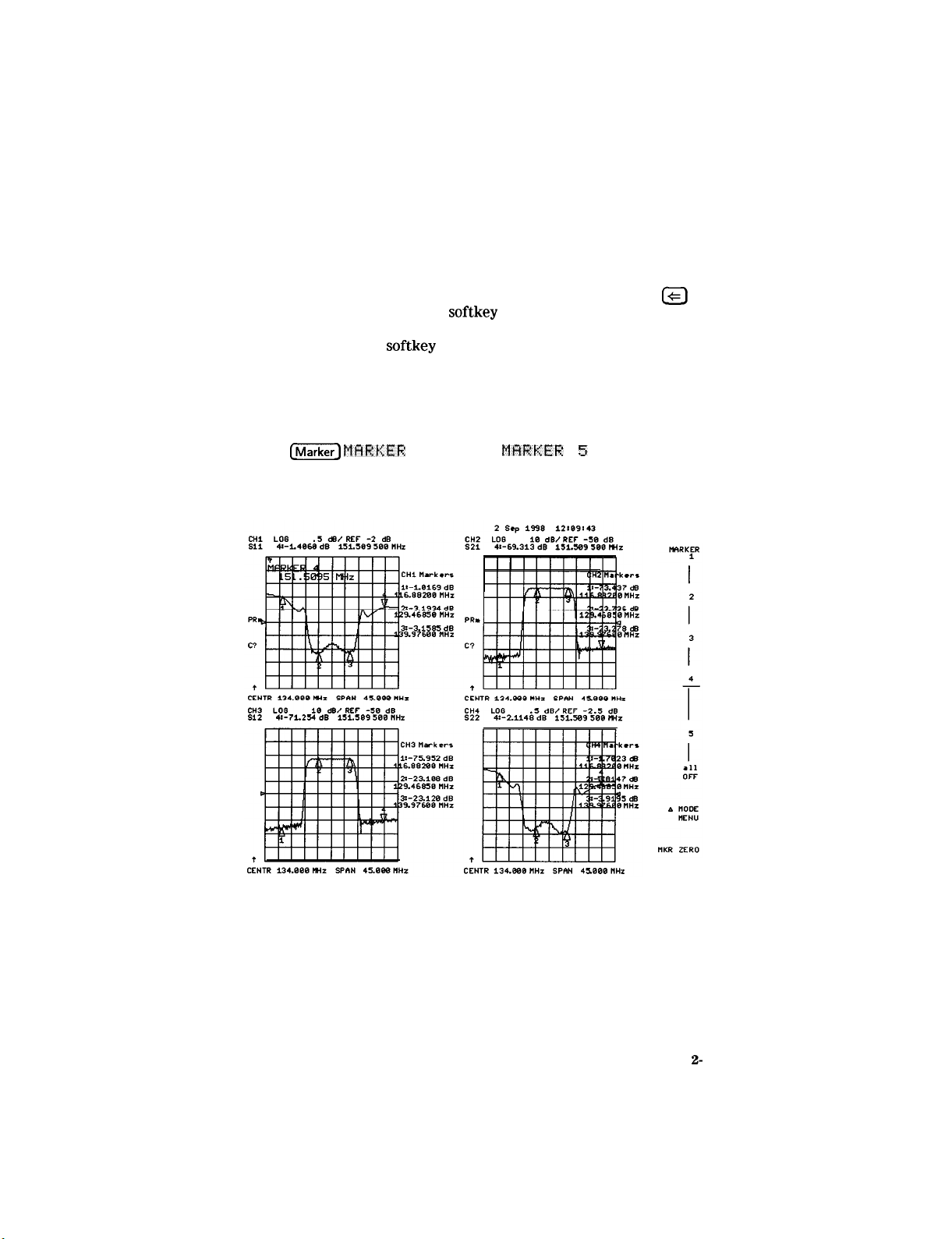
To Move Marker Information off of the Graticules
1. Activate markers 1 through 5:
1 through
Press
(j-1
MHRKER
The display will appear similar to Figure 2-5.
softkey
display on and off and, if more
MHRtCER 5
Figure 2-5. Markers before Pressing the Backspace Key
Making Measurements
2-
11
Page 34

2.
Press
@
The display will appear similar to Figure 2-6. Notice that the marker
information has moved off of channels’ 2 and 4 graticules and into the
softkey display area.
CH4 “arkerr
ir-1.7885 dG
116.882QQ
MHZ
Z-38129 dG
123.46898
tlHZ
3:-3.9114 dG
i39.97688 tlk
CEHTR 134.888 MZ
SPAN
45.888
NHz
*
CEHTR i34.@38lWz
SPAN 45.8BBMHz
Figure 2-6. Markers after Pressing the Backspace Key
To Move Marker Information back onto the Graticules
3.
Press
@.
Notice that the marker information moves back onto the graticules
and that the
softkey
hardkey
2- 12
Making Measurements
softkey
menu is also restored when a
menu is restored as shown in Figure 2-6. The
softkey
or
hardkey
must be one which opens a menu, such as
is pressed. The
CE]
or
Lsystem).
Page 35

l&sting
A Device with Limit Lines
Creating Flat Limit Lines
In this example procedure, the following flat limit line values are set:
Frequency Range . . . . . . . . . . . . . . . . . . . . . . . . . . . . . . . . . . . Power Range
127
MHz to 140 MHz.. . . . . . . . . . . . . . . . . . . . . . . . . . . . . . -27 dB to -21
100 MHz to 123 MHz.. . . . . . . . . . . . . . . . . . . . . . . . . . . . -200 dB to -65
146 MHz to 160 MHz.. . . . . . . . . . . . . . . . . . . . . . . . . . . . . . -200 dB to -65
dB
dB
dB
Note
1. ‘lb access the limits menu and activate the limit lines, press:
2
lb create a new limit line, press:
The analyzer generates a new segment that appears on the center of
the display.
3.
‘lb
specify the limit’s stimulus value, test limits (upper and lower),
and the limit type, press:
Note
The minimum value for measured data is -200
You could also set the upper and lower limits by using
the p1
IDDLE
use these keys for the entry, press:
M
I D D
L E
DELTH LIMITS@@
This would correspond to a test specification of -24
f3 dB.
‘4FlLlJE
6’ H
L U E
and
1-24) @
DELTH
LIMITS keys. lb
dB.
4. lb define the limit as a flat line, press:
L
I
M
I TT ‘i’ P
E FL H T
L
I
t.1
E R E TURN
Making Measurements 2-13
Page 36

5. lb terminate the flat line segment by establishing a single point limit,
press:
Figure 2-7 shows the flat limit lines that you have just created with
the following parameters:
w
stimulus from 127 MHz to 140 MHz
n
upper limit of -21
n lower limit of -27
dB
dB
aw000010
Figure 2-7. Example Flat Limit Line
6. ‘lb create a limit line that tests the low side of the filter, press:
FID[)
!s T I PI l-1 L 1-l !;
tJPPER
LClWEl?
D III 14 E
L I td I TT 7’ P
il D D
!;T IMIJLIJ!~
D 0 t4
E
L I tl I T
2-14 Making Measurements
VHLIJE mm
LIMITa
LIMIT
(-2oo_)@
E FL H T
‘6’ 17
L U E
TYPE SINGLE
L I NE I? E T U R
1123_) m
F’O
I MT
bl
RETURN
Page 37

7.
To
create a limit line that tests the high side of the
press:
bandpass
filter,
LIMIT TYPE FLAT LI
H Cl Cl
!;TIMiJLlJS
DfJHE
LIMIT TYPE
‘v’ 13
L U E
1160_) m
SIHGLE POIt.iT F3ETURt.I
Figure 2-8. Example Flat Limit Lines
t.+E RETURt.1
Making Measurements
2-15
Page 38

Creating a Sloping Limit Line
This example procedure shows you how to make limits that test the
shape factor of a SAW Elter. The following limits are set:
Frequency Range . . . . . . . . . . . . . . . . . . . . . . . . . . . . . . . . . . . . . . . Power Range
123 MHz to 125 MHz . . . . . . . . . . . . . . . . . . . . . . . . . . . . . . . . -65 dB to -26 dB
144
MHz
to 146 MHz . . . . . . . . . . . . . . . . . . . . . . . . . . . . . . . . -26 dB to -65
1. lb access the limits menu and activate the limit lines, press:
dB
@jG)LIMIT
PlEMJ
LIMIT LINE
OH
EDIT LIMIT
LIHE
CLEMR LISTYES
2. ‘lb establish the start frequency and limits for a sloping limit line that
tests the low side of the filter, press:
HDD
LIMIT TYPE
SLOPI HG
L I HE RETURN
3. ‘lb terminate the lines and create a sloping limit line, press:
HDD
ST1
MULUS VHLUE @m
UPPER
LrJWER LIMIT
D B F4
LIMIT TYPE
LIMIT I-26J@
E
SIt4lI;LE
1-2oo_)a
PO1 HT
RETUFrH
2- 16
Making Measurements
Page 39

4. ‘lb establish the start frequency and limits for a sloping limit line that
tests the high side of the Elter, press:
5.
lb terminate the lines and create a sloping limit line, press:
H[>D
LIMIT
You could use this type of limit to test the shape factor of a
TYPE SIHGLE
POIHT
F.:ETURH
filter.
Figure 2-9. Sloping Limit Lines
Making Measurements 2-17
Page 40

Creating Single Point Limits
In this example procedure, the following limits are set:
from -23 dB to -28.5 dB at 141 MHz
from -23 dB to -28.5 dB at 126.5 MHz
1. lb access the limits menu and activate the limit lines, press:
~~]LIMIT
CLEHR LIST ‘r’E:s
2.
‘lb
designate a single point limit line, as shown in Figure 2-10, you
must
deEne
l
downward pointing, indicating the upper test limit
n
upward pointing, indicating the lower test limit
Press:
t4EHU LIMfT
two pointers:
LINE OH
EDIT
LIMIT
LINE
2-18
Making
Measurements
Page 41

aw000013
Figure 2-10. Example Single Point Limit Lines
Making Measurements 2-19
Page 42

Editing Limit Segments
This example shows you how to edit the upper limit of a limit line.
1. ‘lb access the limits menu and activate the limit lines, press:
=LItlIT
2. ‘lb move the pointer symbol
MENU
LfHIT LIHE
(>)
on the analyzer display to the
KU4
EDIT
LIHIT LINE
segment you wish to modify, press:
SE G ME H T @)
or @j repeatedly
OR
$
E C; tl
E t4
T and enter the segment number followed by
3.
‘Ib
change the upper limit (for example, -20) of a limit line, press:
EDIT IJPPER
LIMIf~~f)Ot~IE
@).
Deleting Limit Segments
1. lb access the limits menu and activate the limit lines, press:
~LIMIT
2. lb move the pointer symbol
MEElCl
LIMIT
(>)
on the analyzer display to the
LINE OH
EDIT LIMIT
LIHE
segment you wish to delete, press:
SEC;
tl
E H
T @)
or Q repeatedly
OR
S
EG tl
E
H
T and enter the segment number followed by (xl.
3. ‘lb delete the segment that you have selected with the pointer
symbol, press:
DELETE
2-20 Making Measurements
Page 43

Running a Limit Test
1. lb access the limits menu and activate the limit lines, press:
[~~LIPIIT
Reviewing the Limit Line Segments
The limit table data that you have previously entered is shown on the
analyzer display.
2. lb verify that each segment in your limits table is correct, review the
entries by pressing:
SEGMENT
3. lb modify an incorrect entry, refer to the “Editing Limit Segments”
procedure, located earlier in this section.
@-j
MENIJ
and
LIMIT LINE
@
Qt4
EDIT
LIMIT
LIHE
Activating the Limit
Test
4. lb activate the limit test and the beep fail indicator, press:
0 1.4
[j)
0
Note
L I M
I T
ME
1.4 CI
L I tl
I T
T E 5 T
Selecting the beep fail indicator BEEP
BEEPF H
I L
F R I L
1.4
0 14
is
optional and will add approximately 50 ms of sweep
cycle time. Because the limit test will still work if the
limits lines are off, selecting L I
tl
I T
If4EOH
is
L
also optional.
The limit test results appear on the right side on the analyzer display.
The analyzer indicates whether the filter passes or fails the defined
limit test:
q
The message
FH
I L
will appear on the right side of the display if
the limit test fails.
q
The analyzer beeps if the limit test fails and if BEEP
F H I L
0 t4
has been selected.
q
The analyzer alternates a red trace where the measurement trace is
out of limits.
q
A TTL signal on the rear panel BNC connector “LIMIT TEST”
provides a pass/fail (5
V/O
V) indication of the limit test results.
Making Measurements 2-21
Page 44
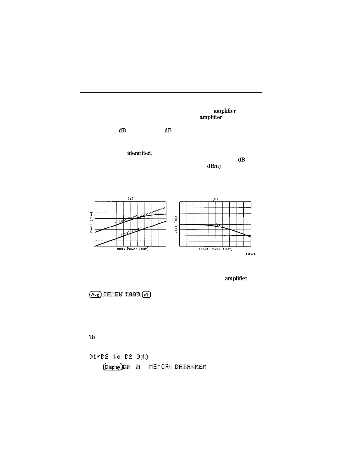
Measuring Gain Compression
Gain compression occurs when the input power of an
increased to a level that reduces the gain of the
amplifier
ampliEer
is
and causes
a nonlinear increase in output power. The point at which the gain
is reduced by 1 dB is called the 1 dB
compression point. The gain
compression will vary with frequency, so it is necessary to End the
worst case point of gain compression in the frequency band.
Once that point is
that CW frequency to measure the input power at which the 1
compression occurs and the absolute power out (in
identiEed,
you can perform a power sweep of
dB
dBm)
at compression.
The following steps provide detailed instruction on how to apply various
features of the analyzer to accomplish these measurements.
Input Power (dh)
Figure 2-11. Diagram of Gain Compression
1. Set up the stimulus and response parameters for your
amplifier
under test. lb reduce the effect of noise on the trace, press:
2. Perform the desired error correction procedure. Refer to Chapter 5,
“Optimizing Measurement Results,” for instructions on how to make
a measurement correction.
3. Hook up the amplifier under test.
4.
‘Ib
produce a normalized trace that represents gain compression,
perform either step 5 or step 6. (Step 5 uses trace math and
step 6 uses uncoupled channels and the display function
Et 2
D 1 .* D 2t.
5.
Press
13
(jw) DH
III 1.1.)
--+ME~~I~IRY DHTH..~‘MEM
T H
to produce a
normalized trace.
2-22 Making Measurements
Page 45

6.
‘lb
produce a normalized trace, perform the following steps:
a. Press
~~~D!JHL:
SETIJP and set
CslJHL C:HHt4
on OFF to
QIJHD
OH
to view channels 1 and 2
simultaneously.
b. ‘lb uncouple the channel stimulus so that the channel power will
be uncoupled, press:
IMenu) COlfPLET) CH CtFF
This will allow you to separately increase the power for
channel 2 and channel 1, so that you can observe the gain
compression on channel 2 while channel 1 remains unchanged.
c. ‘lb display the ratio of channel 2 data to channel 1 data on the
channel 2 display, press:
(Chan2)(-)
0 N
7. Press
. This produces a trace that represents gain compression only.
(W)
MBRE
and set DF:,Dl t,o
D2
on
OFF
MARKER1 and position the marker at approximately
mid-span.
8.
Press(j)SCHLE~DIV(iJ@iJtochangethescaletoldB
per division.
9. Press
IMenu)
F’rJWER.
10. Increase the power until you observe approximately 1 dB of
compression on channel 2, using the step keys or the front panel
knob.
to
11. ‘lb locate the worst case point on the trace, press:
(Marker) MKR
SE
HRCH SEHRCH: Pl
I
N
Making Measurements 2-23
Page 46

CHI S21II og
PRmPRm
C?C?
tt
CHl
START
CHl START
DZ/
DZ/
PRmPRm
C?C?
I
CHZ
START
MAGogMAG
1.000
1.000 000
I I I
1.000 000
000
10 dB/10
MHz
MHz
MHz
dB/
REFREF 0
I
I
Figure 2-12.
Gain Compression using Linear Sweep
dB0dB 1
STOP100E. 000 000
STOP100E. 000 000
19.723
19.723
dB1
I I I I I
STOP 1 000.000 000
and 1321
D 1 t, 0 D
MHz
dB
MHz
MHz
2 ij
t.4
12. If C 0 IJ P
L E
D
I:
H0
F F
was selected, recouple the channel
stimulus by pressing:
[Menu)
13. lb place the marker
tMarkerFctn_) MHRKEE
14.
‘lb
COIJF3LED
IX ON
exuctl~
MODE
on a measurement point, press:
MENlJ MHRKERS: DIS’C:RETE
set the CW frequency before going into the power sweep mode,
press:
Iseq) $iPEC: I AL FiJNl:T 1ljt.j:; MHRI(ER + CL4
15. Press
16.
m
SWEEP TYPE
MEPIIJ POWEFF: SWEEF’.
Enter the start and stop power levels for the sweep.
Now channel 1 is displaying a gain compression curve. (Do not pay
attention to channel 2 at this time.)
2-24
Making Measurements
Page 47
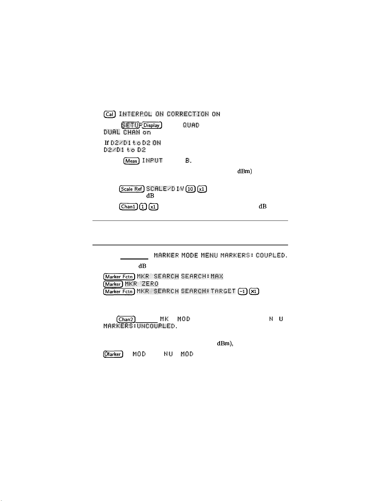
17. ‘lb maintain the calibration for the CW frequency, press:
Icar] ItdfERPrJL I3t.I C~;~RREt;‘fTOb~ Ok+
18.
Press
[jj[j]
SETIJP and set
I)LiftL CXHk4 art
19.
IfD2YDl to D2 rJt.4
DZ,Cfl f,o
I32
DUAL: QUAI>
OFF to ON.
was selected, press MORE
OFF.
20. Press
Now channel 2 displays absolute output power (in
Ihneas) IHPIJT
PORTS
B.
dBm)
as a
function of power input.
2 1.
Press
[Scale]
SlZHLE1D IV
Ilo]@
to change the scale of
channel 2 to 10 dB per division.
22. Press
m
@ Ixl) to change the scale of channel 1 to 1 dB per
division.
Note
A receiver calibration will improve the accuracy of
this measurement. Refer to Chapter 5, “Optimizing
Measurement Results.”
23. Press (Marker)
IIARKER MClDE MEt,+U MHRKERS: C:OIJPLED.
24. ‘lb find the 1 dB compression point on channel 1, press:
Notice that the marker on channel 2 tracked the marker on
channel 1.
25. Press
[Chan2]
[Marker) M K
ME t4
MFIRKERS:
IJHCrSUPLED.
R
E
UM 0 I>
26. lb take the channel 2 marker out of the A mode so that it reads the
absolute output power of the amplifier (in
@iii)
A
I:1
F F
td 0 I> Etl E td U AM 0 I)
E
dBm),
press:
Making Measurements 2-25
Page 48

CHl Szl
PRm
C?
t
CHZ
PRm
t
log MFlG
I I
B
log MFlG
2 dB/ REF 19.01
I
5 dB/ REF 0
dB
dB1 -.
I
1: 7.6474
9956
x
dB
I
dB
START -25. 0 dBm CW
Figure 2-13. Gain Compression using Power Sweep
2-26 Making Measurements
1.000 000
MHz
STOP
0.0 dBm
Page 49

Measurements using the Swept List Mode
Stepped
Swept List Mode
The ability to completely customize the frequency sweep while using
swept list mode is useful when setting up a measurement for a device
with high dynamic range, like a Elter. The following measurement of a
filter illustrates the advantages of using the swept list mode.
Note
List
Mode
Primary channels 1 and 2 can be set up independently
from each other with different frequency
lists (stepped or swept). Press m and set
CrJClPLED
primary channels from each other. You can then
create an independent frequency list for each primary
ChaMel.
Due to the permanent stimulus coupling between
primary and auxiliary channels, channel 3 and 4 will
have the same frequency lists as channels 1 and 2
respectively.
In this mode, the source steps to
each defined frequency point,
stopping while data is taken. This
mode eliminates IF’ delay and allows
frequency segments to overlap.
However, the sweep time can be
substantially slower than for a
continuous sweep with the same
number of points.
This mode takes data while sweeping
through the defined frequency
segments, increasing throughput by
up to 6 times over a stepped sweep.
In addition, this mode allows the test
port power and IF bandwidth to be
set independently for each segment
that is defined. The frequency
segments in this mode cannot
overlap.
CW ljt.4 af f
to OFF to uncouple the
Making Measurements 2-27
Page 50

Connect the Device Under
1. Connect the equipment as shown in the following illustration:
Figure 2-14. Swept List Measurement Setup
2. Set the following measurement parameters:
!521 (B/R>
Test
2-28 Making Measurements
Page 51

Observe the Characteristics of the Filter
CENTER
900.000
500.000
000
MHZ
SPAN
000
MHZ
Figure 2-15. Characteristics of a Filter
w
Generally, the pass band of a Elter exhibits low loss. A relatively low
incident power may be needed to avoid overdriving the next stage of
the DUT (if that stage contains an
ampliEer)
or the network analyzer
receiver.
n
Conversely, the stop band of a filter generally exhibits high isolation.
‘lb measure this characteristic, the dynamic range of the system will
have to be maximized. This can be done by increasing the incident
power and narrowing the IF bandwidth.
Making Measurements 2-29
Page 52
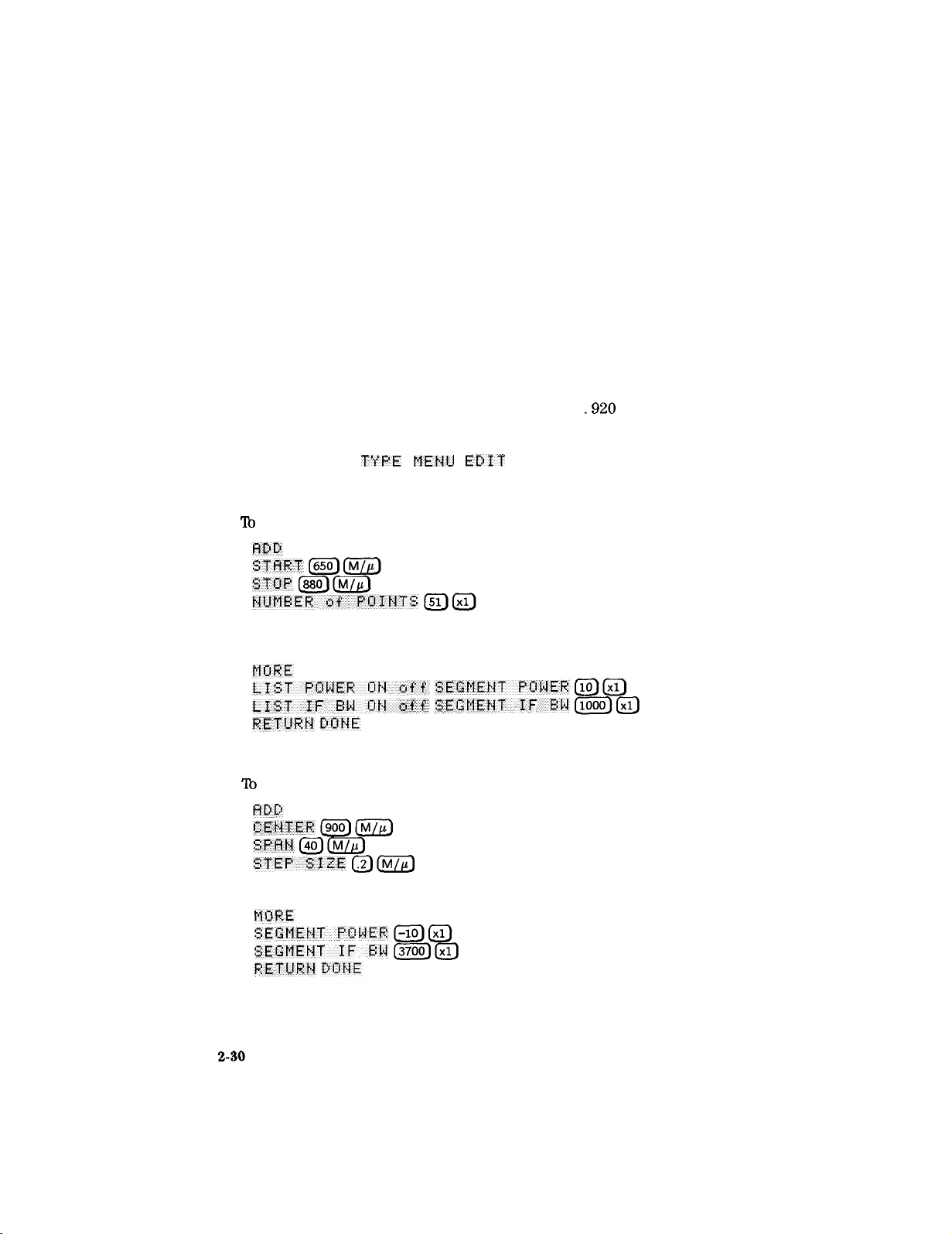
Choose the Measurement Parameters
1. Decide the frequency ranges of the segments that will cover the stop
bands and pass band of the filter. For this example, the following
ranges will be used:
Lower stop band . . . . . . . . . . . . . . . . . . . . . . . . . . . . . . . . . . . . 650 to 880 MHz
880
Pass band
. . . . . . . . . . . . . . . . . . . . . . . . . . . . . . . . . . . . . . . . . . .
Upper stop band.. . . . . . . . . . . . . . . . . . . . . . . . . . . . . . .
2. ‘lb set up the swept list measurement, press
(Menu) SWEEP T-
‘I’F’E MEHIJ EDIT
LIST
Set Up the Lower Stop Band Parameters
3.
‘lb
set up the segment for the lower stop band, press
4. lb maximize the dynamic range in the stop band (increasing the
incident power and narrowing the IF bandwidth), press
to 920 MHz
.920
to 1150 MHz
Set Up the Pass Band Parameters
5.
‘lb
set up the segment for the pass band, press
6.
‘lb specify a lower power level for the pass band, press
Z-30
Making Measurements
Page 53

Set Up the Upper Stop Band Parameters
7. ‘lb set up the segment for the upper stop band, press
H D D
8. ‘lb maximize the dynamic range in the stop band (increasing the
incident power and narrowing the lF bandwidth), press
9. Press
[SONE
LIST
FF?EL!
[SWEPTI.
Calibrate and Measure
1. Remove the DUT and connect a thru between the test ports.
2. Perform a full two-port calibration. Refer to Chapter 5, “Optimizing
Measurement Results.”
3. With the thru connected, set the scale to autoscale to observe the
benefits of using swept list mode.
n
The segments used to measure the stop bands have less noise, thus
maximizing dynamic range within the stop band frequencies.
H
The segment used to measure the pass band has been set up for
faster sweep speed with more measurement points.
Making Measurements 2-3 1
Page 54

CENTER
000.000 000 MHZ SPAN
500.000 000
MtiZ
Figure 2-16. Calibrated Swept List Thru Measurement
4. Reconnect the filter and adjust the scale to compare results with the
first filter measurement that used a linear sweep.
n
In Figure 2-18, notice that the noise level has decreased over
10
dB, confirming
that the noise reduction techniques in the stop
bands were successful.
w
In Figure 2-18, notice that the stop band noise in the third segment
is slightly lower than in the first segment. This is due to the
narrower IF bandwidth of the third segment (300 Hz).
2-32 Making Measurements
Page 55

CENTER 900.000 000 MHZ
SPAN
500.000 000 MHZ
Figure 2-17.
Filter Measurement using Linear Sweep
(Power: 0
dBm/IP BW:
3700 Hz)
Making Measurements 2-33
Page 56

,
loa
CHI
s2:
PRrn
CO!-
CENTER 900.000 000
MAG
m
-
SEGMENT I
Power: +I 0 dBm
IF BW: 1000 Hz
II
MHz
d0,
REF
I
I I
SEGZNT
0
I
dB
SPAN
2
500.000 000 MHZ
SEGMENT 3
Power:
+I0
IF BW: 300 Hz
dBm
Power: -10 dBm
IF BW: 3700 Hz
Figure 2-18. Filter Measurement using Swept List Mode
pge51 e
2-34 Making Measurements
Page 57

3
Making Mixer Measurements
Measurement Considerations
To
ensure successful mixer measurements, the following measurement
challenges must be taken into consideration:
w
Mixer Considerations
q
Minimizing Source and Load Mismatches
q
Reducing the Effect of Spurious Responses
q
Eliminating Unwanted Mixing and Leakage Signals
n
Analyzer Operation
q
How RF and IF Are Defined
q
Frequency Offset Mode Operation
q
Differences Between Internal and External R Channel Inputs
q
Power Meter Calibration
Minimizing Source and Load Mismatches
When characterizing linear devices, you can use vector accuracy
enhancement to mathematically remove all systematic errors, including
source and load mismatches, from your measurement. This is not
possible when the device you are characterizing is a mixer operating
over multiple frequency ranges. Therefore, source and load mismatches
are not corrected for and will add to overall measurement uncertainty.
You should place attenuators at all of the test ports to reduce the
measurement errors associated with the interaction between mixer port
matches and system port matches. ‘lb avoid overdriving the receiver,
you should give extra care to selecting the attenuator located at the
mixer’s IF port. For best results, you should choose the attenuator value
so that the power incident on the analyzer R channel input is less than
-10
dBm
and greater than -35
dBm.
Making Mixer Measurements 3-l
Page 58

Reducing the Effect of Spurious Responses
By choosing test frequencies (frequency list mode), you can reduce the
effect of spurious responses on measurements by avoiding frequencies
that produce IF signal path distortion.
Eliminating Unwanted Mixing and Leakage Signals
By placing filters between the mixer’s IF port and the receiver’s input
port, you can eliminate unwanted mixing and leakage signals from
entering the analyzer’s receiver. Filtering is required in both fixed and
broadband measurements. Therefore, when conIiguring broad-band
(swept) measurements, you may need to trade some measurement
bandwidth for the ability to more selectively filter signals entering the
analyzer receiver.
How RF and IF Are Defined
In standard mixer measurements, the input of the mixer is always
connected to the analyzer’s RF source, and the output of the mixer
always produces the lF frequencies that are received by the analyzer’s
receiver.
However, the ports labeled RF and IF on most mixers are not
consistently connected to the analyzer’s source and receiver ports,
respectively. These mixer ports are switched, depending on whether a
down converter or an up converter measurement is being performed.
It is important to keep in mind that in the setup diagrams of the
frequency offset mode, the analyzer’s source and receiver ports are
labeled according to the mixer port that they are connected to.
n
In a down converter measurement where the D 12 W
El
C rJ N 5’
E RT E
softkey is selected, the notation on the analyzer’s setup diagram
indicates that the analyzer’s source frequency is labeled RF,
connecting to the mixer RF port, and the analyzer’s receiver
frequency is labeled IF, connecting to the mixer IF port.
Because the RF frequency can be greater or less than the set LO
frequency in this type of measurement, you can select either
F:F >
Lo or RF .<
3-2 Making Mixer Measurements
t-111.
R
Page 59
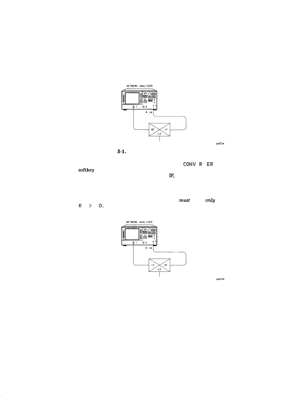
Figure
n
In an up converter measurement where the UP
3-l.
Down Converter Port Connections
C: 0 t.1’4
E R T
El?
softkey is selected, the notation on the setup diagram indicates that
the analyzer’s source frequency is labeled
IF,
connecting to the
mixer IF port, and the analyzer’s receiver frequency is labeled RF,
connecting to the mixer RF port.
Because the RF frequency will always be greater than the set
LO frequency in this type of measurement, you
I?
F > L
0.
must
select
on&
Figure 3-2. Up Converter Port Connections
Making Mixer Measurements 3-3
Page 60

Frequency Offset Mode Operation
Frequency offset measurements do not begin until all of the frequency
offset mode parameters are set. These include the following:
n
Start and Stop IF Frequencies
n
LO frequency
w
Up Converter / Down Converter
H RF>LO/RF<LO
The LO frequency for frequency offset mode must be set to the same
value as the external LO source. The offset frequency between the
analyzer source and receiver will be set to this value.
When frequency offset mode operation begins, the receiver locks onto
the entered IF signal frequencies and then offsets the source frequency
required to produce the IF. Therefore, since it is the analyzer receiver
that controls the source, it is only necessary to set the start and stop
frequencies from the receiver.
Differences Between Internal and External R Channel Inputs
Due to internal losses in the analyzer’s test set, the power measured
internally at the R channel is 16 dB lower than that of the source.
compensate for these losses, the traces associated with the R channel
have been offset 16 dB higher. As a result, power measured
at the R channel via the R CHANNEL IN port will appear to be 16
higher than its actual value. If power meter calibration is not used, this
offset in power must be accounted for with a receiver calibration before
performing measurements.
‘Ib
directly
dB
3-4 Making Mixer Measurements
Page 61

Power Meter Calibration
Mixer transmission measurements are generally conligured as follows:
measured output power
(Watts)
/set input power (Watts)
OR
measured output power
For this reason, the set input power must be accurately controlled in
order to ensure measurement accuracy.
Higher measurement accuracy may be obtained through the use of
power meter calibration. You can use power meter calibration to correct
for power offsets, losses, and
analyzer source and the input to the mixer under test.
(dBm) -
tlatness
set input power
variations occurring between the
(dBm)
Making Mixer Measurements
3-6
Page 62

Conversion Loss using the Frequency Offset Mode
Conversion loss is the measure of efficiency of a mixer. It is the ratio
of side-band IF power to RF signal power, and is usually expressed in
dB.
(Express ratio values in dB amounts to a subtraction of the
power in the denominator from the dB power in the numerator.) The
mixer translates the incoming signal, (RF), to a replica, (IF), displaced
in frequency by the local oscillator, (LO). Frequency translation is
characterized by a loss in signal amplitude and the generation of
additional sidebands. For a given translation, two equal output signals
are expected, a lower sideband and an upper sideband.
Figure 3-3.
An Example Spectrum of RF, LO, and IF Signals Present in a
Conversion Loss Measurement
dB
The analyzer allows you to make a swept RF/IF conversion loss
measurement holding the LO frequency fixed. You can make this
measurement by using the analyzer’s frequency offset measurement
mode. This mode of operation allows you to offset the analyzer’s source
by a fixed value, above or below the analyzer’s receiver. That is, this
allows you to use a device input frequency range that is different from
the receiver input frequency range.
The following procedure describes the swept IF frequency conversion
loss measurement of a broadband component mixer:
1. Set the LO source to the desired CW frequency and power level.
CW frequency = 1000
Power = 13
3-6 Making Mixer Measurements
dBm
MHz
Page 63

2. Set the desired source power to the value which will provide
-10
dBm
or less to the R channel input. Press:
(Menu)
POWER
3. Calibrate and zero the power meter.
4. Connect the measurement equipment as shown in Figure 3-4.
PWW RHNGE Mi3t.I @a
Caution
‘lb prevent connector damage, use an adapter (BP
part
number 1250-1462) as a connector saver for R
CHANNEL IN,
PCWER
SENSOR
Figure 3-4. Connections for R Channel and Source Calibration
5. From the front panel of the BP 87533, set the desired receiver
frequency and source output power by pressing:
B
Istart)(iEJ@Jij
IStop_l@zJm
FREtS! OFFS ON
(MenuJ POWER @a
I NSTRUIlEt4T
MCIDE Ft?EIS!
OFFS
IlENIJ
6. ‘lb view the measurement trace, press:
m
I 11 F’ UT
P 0 F?
T S
I%
7. Select the BP 87533 as the system controller:
Making Mixer Measurements 3-7
Page 64

8. Set the power meter’s address:
BET HDDRESSE!;
H[>DRESS:
P
MTR....‘HP
IE
c##_l(xl_l
9. Select the appropriate power meter by pressing
PrJWER
(HP
436A
MTR C
or HP
1 until the correct model
438At437).
mrmber
is displayed
10. Press
C
listed on the power sensor.
CAL
Ical) PWRNTR
t3L
F FIG
FACfQR
TO RSE
Ixx] @
C:HL LOSSJSE~~:~R
tA5
Cl RFi and enter the correction factors as
Press HD D
DUNE
for each correction factor. When
LISTS
FR E Q U E t4 C ‘f Ixx]
m
finished, press Er U HE .
11. lb perform a one sweep power meter calibration over the IF
frequency range at 0
dBm,
press:
12. ‘lb calibrate the R channel over the IF range, press:
Once completed, the display should read 0
dBm.
3-8 Making Mixer Measurements
Page 65

13. Make the connections as shown in Figure 3-5 for the one-sweep
power meter calibration over the RF range.
NElWRR ARALYYfER
Figure 3-5.
Connections for a One-Sweep Power Meter Calibration for Mixer
Measurements
14. lb set the frequency offset mode LO frequency from the analyzer,
press:
I
HSTRUMEHT
FF;EB I:IFF!~
L 0M
E N U F I? E Q U E
15.
‘lb
select the converter type and a high-side LO measurement
configuration, press:
PlODE
tfEk+lJ
t.4 c;Y
:
CbJ m
m
Making Mixer Measurements 3-9
Page 66

Figure 3-6. Measurement Setup from Display
16. lb view the measurement trace, press:
‘$1 EM PK3iSlJRE
17. ‘lb perform a one-sweep power meter calibration over the RF
frequency range, press:
Ical] FWRMTR CHL
ONE SWEEP
@@
TAKE
CHL
SWEEP
Note
Do not
reduce the number of points to perform this
power meter calibration. Reducing the number of
points will turn off the receiver calibration.
The analyzer is now displaying the conversion loss of the mixer
calibrated with power meter accuracy.
3-10 Making Mixer Measurements
Page 67

18. lb view the conversion loss in the best vertical resolution, press:
Figure 3-7. Conversion Loss Example Measurement
Conversion loss/gain = output power - input power
Making Mixer Measurements
3-l 1
Page 68

High Dynamic Range Swept RF/IF
Conversion Loss
The analyzer has a 35 dB dynamic range limitation on measurements
made directly with its R (phaselock) channel. For this reason, the
measurement of high dynamic range mixing devices (such as mixers with
built in amplification and filtering) with greater than 35 dB dynamic
range must be made on either the analyzer’s A or B channel, with
a reference mixer providing input to the analyzer’s R-channel for
phaselock.
This example describes the swept IF conversion loss measurement of a
mixer and filter. The output filtering demonstrates the analyzer’s ability
to make high dynamic range measurements.
‘lb avoid the complexity of performing a separate power meter
calibration over the RF frequency range while the mixer under test and
reference mixer are operating, a broad band power meter calibration is
used. The broad band calibration covers the entire range of IF and RF
frequencies.
1.
Set the following analyzer parameters:
2. Calibrate and zero the power meter.
3. Connect the measurement equipment as shown in Figure 3-8.
Caution
3-12
Making
lb prevent connector damage, use an adapter (HP
part number 1250-1462) as a connector saver for R
CHANNEL IN.
Mixer Measurements
Page 69

Figure 3-8.
Connections for Broad Band Power Meter Calibration
4. Connect the measurement equipment as shown in Figure 3-9.
Figure 3-9. Connections for Receiver Calibration
5. Set the following analyzer parameters:
Making Mixer Measurements 3-13
Page 70

6. lb calibrate the B channel over the IF range, press:
Once completed, the analyzer should display 0 dBm.
7.
Make the connections shown in Figure 3-10.
8. Set the LO source to the desired CW frequency and power level. For
this example the values are as follows:
n
CW frequency = 1500 MHz
n
source power = 13
dBm
Figure 3-10.
Connections for a High Dynamic Range Swept IF Conversion Loss
Measurement
3-14 Making Mixer Measurements
Page 71

9. ‘lb set the frequency offset mode LO frequency, press:
&iii)
LO
I
t4SfRUtifEt4T PlODE F;REB
MEW FREQUEHCY: c:W (15oo_)m
OFFS
MEt4U
10. ‘lb select the converter type and low-side LO measurement
conhguration,
i?ETURt~j
press:
In this low-side LO, down converter measurement, the analyzer’s
source frequency range will be offset higher than the receiver
frequency range. The source frequency range can be determined
from the following equation:
receiver frequency range (100 to 1000 MHz) + LO frequency
(1500 MHz) = 1.6-2.5
GHz
11. ‘lb view the conversion loss in the best vertical resolution, press:
VI
EM MEHSURE
START
100
000 000
MHZ
STOP1000.000
000
MHZ
Figure 3-11. Example of Swept IF Conversion Loss Measurement
Making Mixer Measurements3-
16
Page 72

Conversion Compression using the Frequency Offset Mode
Conversion compression is a measure of the maximum RF input signal
level, where the mixer provides linear operation. The conversion loss is
the ratio of the IF output level to the RF input level. This value remains
constant over a specified input power range. When the input power
level exceeds a certain maximum, the constant ratio between IF and RF
power levels will begin to change. The point at which the ratio has
decreased 1 dB is called the 1 dB compression point. See Figure 3-12.
Figure 3-12.
Conversion Loss and Output Power as a Function of Input Power
Level Example
Notice that the IF output power increases linearly with the increasing
RF signal, until mixer compression begins and the mixer saturates.
The following example uses a ratio of mixer output to input power and
a marker search function to locate a mixer’s 1 dB compression point.
1. Set the LO source to the desired CW frequency and power level.
CW frequency = 600 MHz
Rower = 13
2. Initialize the analyzer by pressing
3-16 Making Mixer Measurements
dBm
IPreset).
Page 73

3. To set the desired CW frequency and power sweep range, press:
ti
SWEEP
Make the connections, as shown in Figure 3-13.
4.
R
E T U R
t.1
Caution
lb prevent connector damage, use an adapter
(HP
part number 1250-1462) as a connector saver for R
CHANNEL IN.
NETWRN
ANALYZER
Figure 3-13.
Connections for the First Portion of Conversion Compression
Measurement
5. lb view the absolute input power to the analyzer’s R-channel, press:
IMeas) I HPUt PQRTS I?
Making Mixer Measurements 3-17
Page 74

6. ‘lb store a trace of the receiver power versus the source power into
memory and view data/memory, press:
m
DHTM
DHTH.~‘MEtl
+ MEM~3R’f
This removes the loss between the output of the mixer and the
input to the receiver, and provides a linear power sweep for use in
subsequent measurements.
7. Make the connections as shown in Figure 3-14.
Caution
‘lb prevent connector damage, use an adapter (HP
part number
1250-1462)
as a connector saver for R
CHANNEL nv.
Figure 3-14.
Connections for the Second Portion of Conversion Compression
Measurement
8. lb set the frequency offset mode LO frequency, press:
3-18
Making Mixer Measurements
Page 75

9. lb select the converter type, press:
RE-WRN
ILIP r=TJNVERTt%!
10. lb select a low-side LO measurement configuration, press:
RF3
LO
FREG! OFFS OH
In this low-side LO, up converter measurement, the analyzer source
frequency is offset lower than the receiver frequency. The analyzer
source frequency can be determined from the following equation:
receiver frequency (800 MHz) - LO frequency (600 MHz) = 200 MHz
The measurements setup diagram is shown in Figure 3-15.
Figure 3-15.
Measurement Setup Diagram Shown on Analyzer Display
11. lb view the mixer’s output power as a function of its input power,
press:
$‘I El,1 EiEH!;lJRE
12. ‘lb set up an active marker to search for the 1 dB compression point
of the mixer, press:
Making Mixer Measurements 3-19
Page 76

13. Press:
The measurement results show the mixer’s 1 dB compression
point. By changing the target value, you can easily locate other
compression points (for example, 0.5
dB,
3
dB).
See Figure 3-16.
14. Read the compressed power on by turning marker A off.
(jMarker)A
MODE A
MFJDE
OFF
Figure 3-16.
Example Swept Power Conversion Compression
Measurement
3-20 Making Mixer Measurements
Page 77

Isolation Example Measurements
Figure 3-17. Signal Flow in a Mixer Example
Making Mixer Measurements 3-21
Page 78

LO to IF Isolation
NETWRII ANALYZER
Figure 3-18. Connections for a Mixer Isolation Measurement
Figure 3-19.
Example Mixer LO to RF Isolation Measurement
3-22 Making Mixer Measurements
Page 79

RF Feedthrough
Figure 3-20. Connections for a Mixer RF Feedthrough Measurement
Figure 3-21.
Example Mixer RF Feedthrough Measurement
You can measure the IF to RF isolation in a similar manner, but with the
following modifications:
n
Use the analyzer source as the IF signal drive.
D
View the leakage signal at the RF port.
Making Mixer Measurements 3-23
Page 80

Printing, Plotting, and Saving Measurement Results
Configuring a Print Function
1. Connect the printer to the analyzer interface port.
2.
Press
ILocal)
SET
HDDRESSES P[i
C
P R MT R
TYPE
1 until the correct printer choice appears.
3. Select one of the following printer interfaces:
n
ChoosePRNTR PORT
HPLB
interface.
q
Enter the
•I
Press
IJSE PHS!; f;l:lt.+TRaL.
n
Choose P H R H
HP-Ill
address of the printer, followed by
ILocal) SYSTEM CBNTROLLER
C C
L L EL
0 F’ ‘r’
(centronics) interface.
n
Choose
SE
R
I H
L if your printer has a serial
then configure the print function as follows:
B H
U
a. Press P R
I
t.4
T E
rate, followed by
R
Cs
@].
b. ‘lb select the transmission control method that is compatible
with your printer, press X M I T
handshaking protocol) until the correct method appears.
I t4TER PORT
ifyourprinterhasanHP-LR
Ixl).
or
1 if your printer has a parallel
(RS-232)
R H
T E and enter the printer’s baud
C 11
T R L (transmit control
interface, and
-
Printing, Plotting, and Saving Measurement Results
4-l
Page 81

Defining a Print Function
Note
The print definition is set to default values whenever
the power is cycled. However, you can save the print
definition by saving the instrument state.
1. Press
2.
3. Press A UT0 -
m DEFI
Press PR I
f4T:M 0
F E E
HE
PRINT.
t.4
0 12 Ii R 0
tl E
or P R 1
t.4
T :c: 0
D
until the correct choice (ON or OFF) is
L
12 R
.
highlighted.
q
Choose HUT
0
-FE ED0 t4
if you want to print one measurement
per page.
q
Choose R
UT
I:I
-FE ED0
F F if you want to print multiple
measurements per page.
Note
Laser printers and some DeskJet printers do not begin
to print until a full page, or a partial page and a form
feed, have been received.
If You Are Using a Color Printer
1. Press
2. lf you want to modify the print colors, select the print element and
P R I N TC 0 LO R
S .
then choose an available color.
Note
You can set all the print elements to black to create a
hardcopy in black and white.
Since the media color is white or clear, you could set
a print element to white if you do not want that
element to appear on your hardcopy.
‘Ib
Reset the Printing Parameters to Default Values
1. Press
4-2
m
DEFINE
Printing, Plotting, and Saving Measurement Results
PRINT DEFRULT PRt4T
SETUP.
Page 82

Configuring a Plot Function
If You Are Plotting to an
IIPGLIB
Compatible
Printer
2. Press
3. Configure the analyzer for one of the following printer interfaces:
4. Press
ILocal]
SET
P R t4 T
n
Choose
HDDRESSES
T
‘I’P EC
R
PRNTR PORT HF’I
1 until the correct printer choice appears.
PRI
t4TEE
PORT and then press
B
if your printer has an
HP-Ill
interface.
q
Enter the HP-B address of the printer, followed by
C C 0
P 5’
n
Choose PH R H L L E
L
1 if your printer has a parallel
a).
(centronics) interface.
m
Choose S
ER
I HL if your printer has a serial
@S-232)
interface, and
then configure the print function as follows:
B H
U
D R H
T E
a. Press P R
I
ts1 P
E R
and enter the printer’s baud
rate, followed by (xl.
b. ‘lb select the transmission control method that is compatible
with your printer, press
Xt4
I
T R L (transmit control
T
-
C t.1
handshaking protocol) until the correct method appears.
ILocal)
SET
PLTR
ADDRESSES
TYPE
until PLTR TYPE CHPGL PRTI appears.
PLOTTEP.
PrSRT
and then
Printing, Plotting, and Saving Measurement Results 4-3
Page 83

If You Are Plotting to a Pen Plotter
1. Press
ILocal)
PLTE TYPE
SET
ADDF,ESSES
until
PLTli
PLOTTER PORT
TYPE
EPLOTTERI
and
then
appears.
2. Configure the analyzer for one of the following plotter interfaces:
n
Choose PLTR
PORT
HP I B if your plotter has an
HP-IB
interface.
D
Enter the
q
Press
l.jSE F’HSS COWROL.
n Choose PHHHLLEL
m
HP-lE%
address of the plotter, followed by
SYSTEM
C:UtdTROLLER
C
COPY 1 if your plotter has a parallel
or
@.
(centronics) interface.
l
Choose !S
ER
I
WI,
if your plotter has a serial
(RS-232)
interface, and
then configure the print function as follows:
a. Press P R I WE RB H 110
rate, followed by
a).
RATE and enter the plotter’s baud
b. lb select the transmission control method that is compatible
with
your plotter, press X
11
I T
12 11 TR
L (transmit control
-
handshaking protocol) until the correct method appears.
4-4 Printing, Plotting, and Saving Measurement Results
Page 84

If You Are Plotting to a Disk Drive
1. press
2. Press
ILocal) SET FiBDRESSES
[Save/Recall) SELECT
D I 5K
and select the disk drive that you
will plot to.
m
Choose I t4
T E
f? M
disk drive.
n
Choose E X
T E
R H H
external to the analyzer.
PLOTTER
k
L
D f SK
if you will plot to the analyzer internal
L
D
I !2 K if you will plot to a disk drive that is
PORT DISK.
Printing, Plotting, and Saving Measurement Results
4-6
Page 85

Defining a Plot Function
Note
The plot definition is set to default values whenever
the power is cycled. However, you can save the plot
definition by saving the instrument state.
1. Press
@$j
DEFINE PLOT.
Choosing Display Elements
2. Choose which of the following measurement display elements that
you want to appear on your plot:
C”,
I1M
,.ms
Figure
n*
4-l.
Plot Components Available through
SC+ I_yi n
pg6lsod
Definition
Selecting Auto-Feed
3.
Press
HUT 0 -FEED until
q
Choose HUT
0 -
FEED12 N if you
the correct choice is highlighted.
want a “page eject” sent to the
plotter or HPGL compatible printer after each time you press
PLOT.
q
Choose HUT 0
- FEED11 F F
if you want multiple plots on the same
sheet of paper.
rJ H
Note
The peripheral ignores HUT
0
-FEED
are plotting to a quadrant.
4-6 Printing, Plotting, and Saving Measurement Results
when you
Page 86

Selecting Pen Numbers and Colors
4. Press
MQRE
and select the plot element where you want to change
the pen number. For example, press F’ E N NFJ MCs H T H
and then
modify the pen number. The pen number selects the color if you are
plotting to an
HPGL/2
compatible color printer.
Press (xl) after each modification.
Table
4-l.
Default Pen Numbers and Corresponding Colors
Table
4-2. Default Pen Numbers for Plot Elements
Plot Element
Measurement
Data Trace
Displayed
Memory Trace
Graticule and
Reference
Line
Displayed Text
Displayed
Markers and
Values
Printing, Plotting, and
Channel 1
Channel 3
1
Pen Numbers
2
!&wing
Measurement Results 4-7
Channel 2
Channel 4
Pen
Numbers
3
6
Page 87

Note
You can set all the pen numbers to black for a plot in
black and white. You must define the pen numbers for
each measurement channel (channel l/channel 3 and
channel B/channel 4).
Selecting Line Types
5. Press
modify.
MORE
and select each plot element line type that you want to
‘&ble 4-3. Default Line Types for Plot Elements
Plot Elements Channel 1 and 3 Channel 2 and 4
Line Type Numbers Line Type Numbers
Figure 4-2. Line Types Available
4-8
Printing, Plotting, and Saving Measurement Results
Page 88

Choosing Scale
6. Press
SCHLE
q
SCHLE
q
SCHLE PLOT CGRHTI
FLClT
PLOT
until the selection appears that you want.
CFULLJ
Figure 4-3.
Locations of
P1
and P2 in
SCALE PLOT
[ GPHT] Mode
Choosing Plot Speed
7. Press P L I:!
q Choose
q
Choose P L 0 T!Z
transparencies. (The slower speed provides a more consistent line
width.)
T
SPEED until the plot speed appears that you want.
PLOT
SPEED
PEE
D
E
FHST
C S
L 01~11
1 for normal plotting.
for plotting directly on
To
Reset the Plotting Parameters to Default Values
Press
m D
E F
I H
E
F’
L 0 T M
IIt R
E M 0 I? E Cr E F H
l-1 L
T
P
L 0 T !Z E T U P .
If You Are Plotting to an HPGL Compatible Printer
1. Configure and define the plot, as explained in “Configuring a Plot
Function” and “Defining a Plot Function” located earlier in this
chapter.
2. Press
printer has received.
m
PLOT PLOTTER
Printing, Plotting, and Saving Measurement Results 4-9
FOiiM
FEED to print the data the
Page 89

To Save Measurement Results
Note
You can only save measurement data to a disk. The
analyzer internal memory can only store instrument
states and memory traces.
The analyzer stores data in arrays along the processing flow of
numerical data, from IF detection to display. These arrays are points in
the flow path where data is accessible, usually via
HP-II%
You can choose
from three different arrays which vary in modification flexibility when
they’re recalled.
Define Save
Raw Data Array
Data Array
Format Array
Modification Flexibility
During Recall
Most
Medium
Least
You can also save data-only. A data-only file is saved to disk with
default filenames
DATA31D2
DATAOOD4
for channel 2,
to
DATAOODl
DATA31D4
to
DATASlDl
DATAOOD3
for channel 1,
to
DATA31D3
DATAOODB
to
for channel 3, and
for channel 4. However, these files are not
instrument states and cannot be recalled.
4-10
Printing, Plotting, and Saving Measurement Results
Page 90

Figure 4-4. Data Processing Flow Diagram
1. Press (SAVE RECALL) SELECT
D f Sk.
2. Choose one of the following disk drives:
q INTERNAL DISK
q
EXTERMAL DISK
3. PreSS@AVE
RECALL][jEFltdE
DISK-SR’GE.
4. Define the save by selecting one of the following choices:
q
DkTH ARRRY
0
R H wH
o
FORMFIT
0
GRj%PHIt:S 0t.j
o tXi
TH
Note
R R H
D t.1
OH
‘.r’II
t.4
HRRHY OH
L Y0
t.1
(When ON, the other choices are ignored.)
If you select
[:I H
T
13
0 t4
L
‘f
0 td
, you
cannot recall
and display the file contents on the analyzer. This
type of data is intended for computer manipulation.
ErHTH 13+LY 0 t.1
Printing, Plotting,
always saves corrected data.
and
Saving Measurement Results
4-
11
Page 91

5. Choose the type of format you want:
B
I
b1HFrY
q
Choose S R
CITIFILE, S2P,
q
Choose
SHVE
US I NG
YE
or CAE applications.
I
HC;
HS C I
US
for all applications except
I
for
CITlFILE, S2P,
and CAE
applications or when you want to import the information into a
spread sheet format.
6.
Press
RETIJRH SHVE STHTE.
Recalling an Instrument State
1.
Press(S~vE
2. Choose from the following storage devices:
q
1 HTERHAL
q
I
q
EXTERNHL
3. Press the @ repeatedly until the name of the Ele that you want to
recall is high-lighted.
4. Press
REcALLjSELECT DISK.
MEMORY
t.+TERtAtil+ DISK
DISK
RETIJRN RECHLL
STHTE.
412
Printing, Plotting,
and Saving Measurement Results
Page 92

Optimizing Measurement Results
Increasing Measurement Accuracy
Connector Repeatability
H
Inspect the connectors.
w
Clean the connectors.
n
Gauge the connectors.
n
Use correct connection techniques.
Interconnecting Cables
n
Inspect for lossy cables.
H
Inspect for damaged cable connectors.
n
Practice good connector care techniques.
w
Minimize cable position changes between error-correction and
measurements.
Temperature Drift
n
Use a temperature-controlled environment.
n
Ensure the temperature stability of the calibration devices.
N
Avoid handling the calibration devices unnecessarily during
calibration.
w
Ensure the ambient temperature is &lo of measurement calibration
temperature.
Optimizing Measurement Results 5-l
Page 93

Frequency Drift
n
Override the internal crystal with a high-stability external source,
frequency standard, or use the internal frequency standard.
Performance Verification
n
Perform a measurement
veriEcation
at least once per year
Reference Plane and Port Extensions
Use the port extension feature to compensate for the phase shift of an
extended measurement reference plane, due to such additions as cables,
adapters, and Extures, after completing an error-correction procedure
(or when there is no active correction).
Press
Ical) PlrJRE
enter the delay to the reference plane.
PORT
E’ATEMS I CM EXTEN!S IONS
Ot4.
Then
5-2 Optimizing Measurement Results
Page 94

Measurement Error-Correction
Clarifying Type-N
When you are performing error-correction for a system that has type-N
test port connectors, the softkey menus label the sex of the test port
connector label $ HO E TC
female
Response
not
the calibration standard connector. For example, the
F 1
test port.
Error-Correction
Connector
refers to the short that will be connected to the
Sex
for
Reflection
Measurements
1. Select the type of measurement you want to make.
2.
lb select a response correction, press:
TE
Ical]
CHL I
Bf?H
MEW RESPrJtGE
Figure
Standard Connections for a Response Error-Correction for
Reflection Measurement
3. ‘lb measure the standard when the displayed trace has settled, press:
S H 0 R T
or 0 P
E
t.4
5-l.
Optimizing Measurement Results 5-3
Page 95

Response
Error-Correction
for Transmission
Measurements
1. Select the type of measurement you want to make.
2. lb select a response correction, press:
Ical] CRLIBRRTE MEi-ACI RESF‘OWSE
Figure 5-2.
Standard Connections for Response Error-Correction for
Transmission Measurements
3. ‘lb measure the standard, press:
THRU
Response and
Isolation Error-Correction
for
Transmission Measurements
This procedure is intended for measurements that have a measurement
range of greater than 90
1. Select the type of measurement you want to make.
2. lb select a response and isolation correction, press:
Ical] C:HL 1 E:F;HTE tqEt4l-1 REsPi:~t4!2E k
3. Make a
your device under test.
4. lb measure the standard, when the displayed trace has settled, press:
THRCl
5-4 Optimizing Measurement Results
“thru”
connection between the points where you will connect
dB.
I
SOL i t.1 RESPOHSE
Page 96

5. Connect impedance-matched loads to PORT 1 and PORT 2, as shown
in Figure 5-3. Include the adapters that you would include for your
device measurement.
Figure 5-3.
Standard Connections for a Response and Isolation
Error-Correction for Transmission Measurements
6. lb help remove crosstalk noise, set the analyzer as follows:
a. Press
@ R’~,~E~:HGI~K OH HVERHGI t4G
FAI~TOR and enter
at least four times more averages than desired during the device
measurement.
b. Press
Ical) PIORE HLTERHHTE
I? and B
to eliminate one
crosstalk path.
7. ‘lb measure the calibration standard, press:
Ical] RE$lJtlE CflL
SEIJI,JEF.~I:E 1 SOL ’ I.4 S-l-E:I
8. Return the averaging to the original state of the measurement. For
example, reduce the averaging factor by at least four tunes or turn
averaging off.
9.
‘Ib
compute the isolation error coefficients, press:
@
RE$lJME
l:HL
!3EQlJENl:E
Dijt.iE
HE:sP 1
Optimizing Measurement Results 5-5
:sijL ’ t.4
I:HL
Page 97

One-Port Reflection Error-Correction
1. Select the type of measurement you want to make.
2. To select the correction type, press:
Ci3L 1
BRUTE
q
If you want to make a reflection measurement at PORT 1, press:
511
l-FTJRT
q
If you want to make a reflection measurement at PORT 2, press:
!522 1 -PTJRT
Standard Connections for a One-Port Reflection Error-Correction
MEW
and
select the correction type.
NETWKK AWALYZER
Figure 5-4.
q
‘lb
measure the standards in sequence, press:
0 P E t.4
!sHOFs:T
Ll:lHr)
q
lb
compute the error coefficients, press:
~)I:IF~E
:
I-PORT CFiL
6-6
Optimizing Measurement Results
Page 98

Full Two-Port Error-Correction
1. Set any measurement parameters that you want for the device
measurement: power, format, number of points, or IF bandwidth.
2.
lb select the correction type, press:
Ical)
II:HL I BRHTE
MEWJ
FULL
Z-PORT REFLEl:TIOH
FOR REFLECTION FOR TRANSMISSION
FMI
ISOLATION
Figure 5-5.
Standard Connections for Full Two-Port Error-Correction
3. ‘lb measure the standards in sequence, press:
Cl P
E
!s H 11 R
t.4
T
F C! R W H t? D :
F lj R 1~1 H R D :
FORWHRD: LORD
4. Repeat the open-short-load measurements described
above, but connect the devices in turn to PORT 2, and
use the REVERSE:
REVERSE: LOAD softkeys.
ClPEH,
REVERSE:
SHCGrT,
and
5. lb compute the reflection correction coefficients, press:
STHt.jDflRDS Dljt.jE
6. ‘lb start the transmission portion of the correction, press:
T R H t.j!; Pl
7. Make a
1 :; !s 1
III 1.1
“thru”
connection between the points where you
will
connect your device under test as shown in Figure 5-5.
Optimizing Measurement Results 5-7
Page 99

8. ‘lb measure the standard, when the trace has settled, press:
DO
BOTH FWD+REV
9. Press I S 0
q
If you will be measuring devices with a dynamic range less than
90
rdMIT TSOL~TIOt.~
q
lf
than 90
L HT
I 0 H and select from the following two options:
dB,
press:
you will be measuring devices with a dynamic range greater
dB,
follow these steps:
a. Connect impedance-matched loads to PORT 1 and PORT 2.
Include the adapters that you would include for your device
measurement.
b.
Activate at least four times more averages than desired during
the device measurement.
d. Return the averaging to the original state of the measurement,
and press
@
RESUME
C:HL
SEQUENCE.
10. ‘lb compute the error coefficients, press:
D 0 t.4
E
Z-PORT
CML
6-8
Optimizing Measurement Results
Page 100

Power Meter Measurement Calibration
You can use the power meter to monitor and correct the analyzer source
power to achieve calibrated absolute power at the test port. You can
also use this calibration to set a reference power for receiver power
calibration, and mixer measurement calibration.
Note
Loss of Power Calibration Data
If your instrument state has not been saved after a
power meter calibration, the power correction data
will be lost if any of the following circumstances
exists:
n
if you switch off the analyzer ac power and you
haven’t saved the correction in an internal register.
n
if you press
IPreset)
and you haven’t saved the
correction in an internal register.
w
if you change the sweep type (linear, log, list,
CW, power) when the power meter correction is
activated.
=
if you change the frequency when the sweep type is
in log or list mode.
Entering the Power Sensor Calibration Data
Entering the power sensor calibration data compensates for the
frequency response of the power sensor, thus ensuring the accuracy of
power meter calibration.
1. Make sure that your analyzer and power meter are conflgured.
2
~
Press Ical]
SEklSOR fl.
P
l#J R Pl T R
I: H L L III !s :s ./ !S E 1.4
S RL 1s T
S I; H
L F H I: T III R
Compensating for
Directional
Coupler
Response
If you use a directional coupler to sample power in your measurement
configuration, you should enter the coupled arm power loss value into
the power loss table, using the following procedure.
Optimizing Measurement Results 5-9
 Loading...