Agilent 8753E Programming Manual

Download

HP BASIC Programming

Examples Guide

HP 8753E Network Analyzer

Including Option 011

HP Part No. 08753-90413

Printed in USA

January 1998

The information contained in this document is subject to change without notice.

Hewlett-Packard makes no warranty of any kind with regard to this material, including but not limited to, the implied warranties of merchantability and ﬁtness for a particular purpose. Hewlett-Packard shall not be liable for errors contained herein or for incidental or consequential damages in connection with the furnishing, performance, or use of this material.

How to Use This Guide

This guide uses the following conventions:

Front-Panel Key This represents a key physically located on the

instrument.

Softkey This represents a “softkey”, a key whose label is

determined by the instrument ﬁrmware.

Screen Text This represents text displayed on the instrument’s

screen.

HP 8753E/Option 011 Network Analyzer Documentation Map

The Installation and Quick Start Guide familiarizes you with the HP 8753E/Option 011 network analyzer’s front and rear panels, electrical and environmental operating requirements, as well as procedures for installing, conﬁguring, and verifying the operation of the analyzer.

The User’s Guide show how to make measurements, explains commonly-used features, and tells you how to get the most performance from your analyzer.

The Quick Reference Guide provides a summary of selected user features.

The HP-IB Programming Examples Guide provides a tutorial introduction using BASIC programming examples to demonstrate the remote operation of the network analyzer.

The HP BASIC Programming Examples Guide provides a tutorial introduction using BASIC programming examples to demonstrate the remote operation of the network analyzer.

The System Veriﬁcation and Test Guide provides the system veriﬁcation and performance test and the Performance Test Record for your HP 8753E/Option 011 network analyzer.

Contents

1. HP BASIC Programming Examples Guide

Introduction . . . . . . . . . . . . . . . . . . . . . . . . . . . . . . . . . . . . . . . . . . . . . . . . . . . . . . . . . . . . . . . . .10

Required Equipment . . . . . . . . . . . . . . . . . . . . . . . . . . . . . . . . . . . . . . . . . . . . . . . . . . . . . . . .11

Optional Equipment . . . . . . . . . . . . . . . . . . . . . . . . . . . . . . . . . . . . . . . . . . . . . . . . . . . . . .11

System Setup and HP-IB Veriﬁcation. . . . . . . . . . . . . . . . . . . . . . . . . . . . . . . . . . . . . . . . . . .11

HP 8753E Network Analyzer Instrument Control Using BASIC . . . . . . . . . . . . . . . . . . . . . . .14

Command Structure in BASIC . . . . . . . . . . . . . . . . . . . . . . . . . . . . . . . . . . . . . . . . . . . . . . . .14

Command Query. . . . . . . . . . . . . . . . . . . . . . . . . . . . . . . . . . . . . . . . . . . . . . . . . . . . . . . . . . . .16

Running the Program . . . . . . . . . . . . . . . . . . . . . . . . . . . . . . . . . . . . . . . . . . . . . . . . . . . . .16

Operation Complete . . . . . . . . . . . . . . . . . . . . . . . . . . . . . . . . . . . . . . . . . . . . . . . . . . . . . . . . .17

Running the Program . . . . . . . . . . . . . . . . . . . . . . . . . . . . . . . . . . . . . . . . . . . . . . . . . . . . .17

Preparing for Remote (HP-IB) Control . . . . . . . . . . . . . . . . . . . . . . . . . . . . . . . . . . . . . . . . . .18

I/O Paths. . . . . . . . . . . . . . . . . . . . . . . . . . . . . . . . . . . . . . . . . . . . . . . . . . . . . . . . . . . . . . . . . .19

Measurement Process . . . . . . . . . . . . . . . . . . . . . . . . . . . . . . . . . . . . . . . . . . . . . . . . . . . . . . . . .20

Step 1. Setting Up the Instrument . . . . . . . . . . . . . . . . . . . . . . . . . . . . . . . . . . . . . . . . . . . . .20

Step 2. Calibrating the Test Setup . . . . . . . . . . . . . . . . . . . . . . . . . . . . . . . . . . . . . . . . . . . . .20

Step 3. Connecting the Device under Test . . . . . . . . . . . . . . . . . . . . . . . . . . . . . . . . . . . . . . .21

Step 4. Taking the Measurement Data. . . . . . . . . . . . . . . . . . . . . . . . . . . . . . . . . . . . . . . . . .21

Step 5. Post-Processing the Measurement Data. . . . . . . . . . . . . . . . . . . . . . . . . . . . . . . . . . .21

Step 6. Transferring the Measurement Data . . . . . . . . . . . . . . . . . . . . . . . . . . . . . . . . . . . . .21

BASIC Programming Examples . . . . . . . . . . . . . . . . . . . . . . . . . . . . . . . . . . . . . . . . . . . . . . . . .22

Program Information . . . . . . . . . . . . . . . . . . . . . . . . . . . . . . . . . . . . . . . . . . . . . . . . . . . . . . . .23

Analyzer Features Helpful in Developing Programming Routines. . . . . . . . . . . . . . . . . . . .23

Analyzer-Debug Mode. . . . . . . . . . . . . . . . . . . . . . . . . . . . . . . . . . . . . . . . . . . . . . . . . . . . .23

User-Controllable Sweep. . . . . . . . . . . . . . . . . . . . . . . . . . . . . . . . . . . . . . . . . . . . . . . . . . .24

Example 1: Measurement Setup . . . . . . . . . . . . . . . . . . . . . . . . . . . . . . . . . . . . . . . . . . . . . . . . .25

Example 1A: Setting Parameters . . . . . . . . . . . . . . . . . . . . . . . . . . . . . . . . . . . . . . . . . . . . . .25

Running the Program . . . . . . . . . . . . . . . . . . . . . . . . . . . . . . . . . . . . . . . . . . . . . . . . . . . . .26

Example 1B: Verifying Parameters. . . . . . . . . . . . . . . . . . . . . . . . . . . . . . . . . . . . . . . . . . . . .26

Running the Program . . . . . . . . . . . . . . . . . . . . . . . . . . . . . . . . . . . . . . . . . . . . . . . . . . . . .27

Contents

Example 2: Measurement Calibration. . . . . . . . . . . . . . . . . . . . . . . . . . . . . . . . . . . . . . . . . . . . 28

Calibration Kits. . . . . . . . . . . . . . . . . . . . . . . . . . . . . . . . . . . . . . . . . . . . . . . . . . . . . . . . . . . . 28

Example 2A: S11 1-Port Calibration . . . . . . . . . . . . . . . . . . . . . . . . . . . . . . . . . . . . . . . . . . . 29

Running the Program . . . . . . . . . . . . . . . . . . . . . . . . . . . . . . . . . . . . . . . . . . . . . . . . . . . . 30

Example 2B: Full 2-Port Measurement Calibration. . . . . . . . . . . . . . . . . . . . . . . . . . . . . . . 31

Running the Program . . . . . . . . . . . . . . . . . . . . . . . . . . . . . . . . . . . . . . . . . . . . . . . . . . . . 33

Example 2C: Adapter Removal Calibration. . . . . . . . . . . . . . . . . . . . . . . . . . . . . . . . . . . . . . 33

Running the Program . . . . . . . . . . . . . . . . . . . . . . . . . . . . . . . . . . . . . . . . . . . . . . . . . . . . 35

Example 2D: Using Raw Data to Create a Calibration (Simmcal). . . . . . . . . . . . . . . . . . . . 35

Running the Program . . . . . . . . . . . . . . . . . . . . . . . . . . . . . . . . . . . . . . . . . . . . . . . . . . . . 40

Example 2E: Take4 — Error Correction Processed on an External PC. . . . . . . . . . . . . . . . 40

Running the Program . . . . . . . . . . . . . . . . . . . . . . . . . . . . . . . . . . . . . . . . . . . . . . . . . . . . 46

Example 3: Measurement Data Transfer . . . . . . . . . . . . . . . . . . . . . . . . . . . . . . . . . . . . . . . . . 47

Trace-Data Formats and Transfers . . . . . . . . . . . . . . . . . . . . . . . . . . . . . . . . . . . . . . . . . . . . 47

Example 3A: Data Transfer Using Markers . . . . . . . . . . . . . . . . . . . . . . . . . . . . . . . . . . . . . 48

Running the Program . . . . . . . . . . . . . . . . . . . . . . . . . . . . . . . . . . . . . . . . . . . . . . . . . . . . 49

Example 3B: Data Transfer Using FORM 4 (ASCII Transfer). . . . . . . . . . . . . . . . . . . . . . . 50

Running the Program . . . . . . . . . . . . . . . . . . . . . . . . . . . . . . . . . . . . . . . . . . . . . . . . . . . . 52

Example 3C: Data Transfer Using Floating-Point Numbers . . . . . . . . . . . . . . . . . . . . . . . . 53

Running the Program . . . . . . . . . . . . . . . . . . . . . . . . . . . . . . . . . . . . . . . . . . . . . . . . . . . . 54

Example 3D: Data Transfer Using Frequency-Array Information . . . . . . . . . . . . . . . . . . . 55

Running the Program . . . . . . . . . . . . . . . . . . . . . . . . . . . . . . . . . . . . . . . . . . . . . . . . . . . . 57

Example 3E: Data Transfer Using FORM 1 (Internal-Binary Format). . . . . . . . . . . . . . . . 58

Running the Program . . . . . . . . . . . . . . . . . . . . . . . . . . . . . . . . . . . . . . . . . . . . . . . . . . . . 59

Example 4: Measurement Process Synchronization. . . . . . . . . . . . . . . . . . . . . . . . . . . . . . . . . 60

Status Reporting . . . . . . . . . . . . . . . . . . . . . . . . . . . . . . . . . . . . . . . . . . . . . . . . . . . . . . . . . . . 60

Example 4A: Using the Error Queue. . . . . . . . . . . . . . . . . . . . . . . . . . . . . . . . . . . . . . . . . . . 61

Running the Program . . . . . . . . . . . . . . . . . . . . . . . . . . . . . . . . . . . . . . . . . . . . . . . . . . . . 62

Example 4B: Generating Interrupts . . . . . . . . . . . . . . . . . . . . . . . . . . . . . . . . . . . . . . . . . . . 63

Running the Program . . . . . . . . . . . . . . . . . . . . . . . . . . . . . . . . . . . . . . . . . . . . . . . . . . . . 65

Example 4C: Power Meter Calibration . . . . . . . . . . . . . . . . . . . . . . . . . . . . . . . . . . . . . . . . . 66

Contents

Running the Program . . . . . . . . . . . . . . . . . . . . . . . . . . . . . . . . . . . . . . . . . . . . . . . . . . . . .69

Example 5: Network Analyzer System Setups. . . . . . . . . . . . . . . . . . . . . . . . . . . . . . . . . . . . . .70

Saving and Recalling Instrument States . . . . . . . . . . . . . . . . . . . . . . . . . . . . . . . . . . . . . . . .70

Example 5A: Using the Learn String . . . . . . . . . . . . . . . . . . . . . . . . . . . . . . . . . . . . . . . . . . .70

Running the Program . . . . . . . . . . . . . . . . . . . . . . . . . . . . . . . . . . . . . . . . . . . . . . . . . . . . .71

Example 5B: Reading Calibration Data . . . . . . . . . . . . . . . . . . . . . . . . . . . . . . . . . . . . . . . . .72

Running the Program . . . . . . . . . . . . . . . . . . . . . . . . . . . . . . . . . . . . . . . . . . . . . . . . . . . . .74

Example 5C: Saving and Restoring the Analyzer Instrument State. . . . . . . . . . . . . . . . . . .75

Running the Program . . . . . . . . . . . . . . . . . . . . . . . . . . . . . . . . . . . . . . . . . . . . . . . . . . . . .77

Example 6: List-Frequency Tables and Limit-Test Tables . . . . . . . . . . . . . . . . . . . . . . . . . . . .78

Using List Frequency Sweep Mode . . . . . . . . . . . . . . . . . . . . . . . . . . . . . . . . . . . . . . . . . . . . .78

Example 6A1: Setting Up a List Frequency Table In Stepped List Mode. . . . . . . . . . . . . . .79

Running the Program . . . . . . . . . . . . . . . . . . . . . . . . . . . . . . . . . . . . . . . . . . . . . . . . . . . . .80

Example 6A2: Setting Up a List Frequency Table In Swept List Mode . . . . . . . . . . . . . . . .80

Running the Program . . . . . . . . . . . . . . . . . . . . . . . . . . . . . . . . . . . . . . . . . . . . . . . . . . . . .83

Example 6B: Selecting a Single Segment from a Table of Segments . . . . . . . . . . . . . . . . . .84

Running the Program . . . . . . . . . . . . . . . . . . . . . . . . . . . . . . . . . . . . . . . . . . . . . . . . . . . . .85

Using Limit Lines to Perform PASS/FAIL Tests . . . . . . . . . . . . . . . . . . . . . . . . . . . . . . . . . .86

Example 6C: Setting Up a Limit-Test Table. . . . . . . . . . . . . . . . . . . . . . . . . . . . . . . . . . . . . .87

Running the Program . . . . . . . . . . . . . . . . . . . . . . . . . . . . . . . . . . . . . . . . . . . . . . . . . . . . .89

Example 6D: Performing PASS/FAIL Tests While Tuning . . . . . . . . . . . . . . . . . . . . . . . . . .90

Running the Program . . . . . . . . . . . . . . . . . . . . . . . . . . . . . . . . . . . . . . . . . . . . . . . . . . . . .91

Example 7: Report Generation . . . . . . . . . . . . . . . . . . . . . . . . . . . . . . . . . . . . . . . . . . . . . . . . . .93

Example 7A1: Operation Using Talker/Listener Mode . . . . . . . . . . . . . . . . . . . . . . . . . . . . .93

Running the Program . . . . . . . . . . . . . . . . . . . . . . . . . . . . . . . . . . . . . . . . . . . . . . . . . . . . .94

Example 7A2: Controlling Peripherals Using Pass-Control Mode . . . . . . . . . . . . . . . . . . . .95

Running the Program . . . . . . . . . . . . . . . . . . . . . . . . . . . . . . . . . . . . . . . . . . . . . . . . . . . . .97

Example 7A3: Printing with the Serial Port. . . . . . . . . . . . . . . . . . . . . . . . . . . . . . . . . . . . . .98

Running the Program . . . . . . . . . . . . . . . . . . . . . . . . . . . . . . . . . . . . . . . . . . . . . . . . . . . . .99

Example 7B1: Plotting to a File and Transferring the File Data to a Plotter. . . . . . . . . . .100

Contents

Running the Program . . . . . . . . . . . . . . . . . . . . . . . . . . . . . . . . . . . . . . . . . . . . . . . . . . . 101

Utilizing PC-Graphics Applications Using the Plot File. . . . . . . . . . . . . . . . . . . . . . . . . . . 102

Example 7B2: Reading Plot Files From a Disk. . . . . . . . . . . . . . . . . . . . . . . . . . . . . . . . . . 103

Running the Program . . . . . . . . . . . . . . . . . . . . . . . . . . . . . . . . . . . . . . . . . . . . . . . . . . . 108

Example 7C: Reading ASCII Disk Files to the Instrument Controller's Disk File. . . . . . 109

Running the Program . . . . . . . . . . . . . . . . . . . . . . . . . . . . . . . . . . . . . . . . . . . . . . . . . . . 112

Example 8: Mixer Measurements . . . . . . . . . . . . . . . . . . . . . . . . . . . . . . . . . . . . . . . . . . . . . . 113

Example 8A: Comparison of Two Mixers — Group Delay, Amplitude or Phase . . . . . . . . 113

Running the Program . . . . . . . . . . . . . . . . . . . . . . . . . . . . . . . . . . . . . . . . . . . . . . . . . . . 115

Limit Line and Data Point Special Functions. . . . . . . . . . . . . . . . . . . . . . . . . . . . . . . . . . . . . 116

Overview . . . . . . . . . . . . . . . . . . . . . . . . . . . . . . . . . . . . . . . . . . . . . . . . . . . . . . . . . . . . . . . . 117

Example Display of Limit Lines . . . . . . . . . . . . . . . . . . . . . . . . . . . . . . . . . . . . . . . . . . . 118

Limit Segments . . . . . . . . . . . . . . . . . . . . . . . . . . . . . . . . . . . . . . . . . . . . . . . . . . . . . . . . 120

Output Results. . . . . . . . . . . . . . . . . . . . . . . . . . . . . . . . . . . . . . . . . . . . . . . . . . . . . . . . . 121

Constants Used Throughout This Document . . . . . . . . . . . . . . . . . . . . . . . . . . . . . . . . . . . 122

Output Limit Test Pass/Fail Status Per Limit Segment. . . . . . . . . . . . . . . . . . . . . . . . . . . 123

Output Pass/Fail Status for All Segments. . . . . . . . . . . . . . . . . . . . . . . . . . . . . . . . . . . . . . 124

Example Program of OUTPSEGAF Using BASIC. . . . . . . . . . . . . . . . . . . . . . . . . . . . . 124

Output Minimum and Maximum Point Per Limit Segment. . . . . . . . . . . . . . . . . . . . . . . . 126

Output Minimum and Maximum Point For All Segments . . . . . . . . . . . . . . . . . . . . . . . . . 127

Example Program of OUTPSEGAM Using BASIC . . . . . . . . . . . . . . . . . . . . . . . . . . . . 128

Output Data Per Point . . . . . . . . . . . . . . . . . . . . . . . . . . . . . . . . . . . . . . . . . . . . . . . . . . . . . 129

Output Data Per Range of Points. . . . . . . . . . . . . . . . . . . . . . . . . . . . . . . . . . . . . . . . . . . . . 130

Output Limit Pass/Fail by Channel . . . . . . . . . . . . . . . . . . . . . . . . . . . . . . . . . . . . . . . . . . . 131

1 HP BASIC Programming Examples

Guide

HP BASIC Programming Examples Guide

Introduction

This is an introduction to the remote operation of the HP 8753E Network Analyzer using an external controller. This is a tutorial introduction using BASIC programming examples to demonstrate the remote operation of the network analyzer. The examples used in this document are on the “HP 8753E HP BASIC Programming Examples” disk.

The user should be familiar with the operation of the analyzer before attempting to remotely control the analyzer via the Hewlett-Packard Interface Bus (HP-IB). See the HP 8753E Network Analyzer User's Guide for analyzer operating information.

The following computers operating with BASIC 6.2 can be used in these examples:

• HP 9000 Series 200/300

• HP 9000 Series 700 with HP BASIC-UX This document is not intended to teach BASIC programming or to discuss HP-IB theory

except at an introductory level. For more information concerning B ASIC , seeT able 1-1 for a list of manuals supporting the

BASIC revision being used. For more information concerning the Hewlett-Packard Interface Bus, see Table 1-2.

Table 1-1 Additional BASIC 6.2 Programming Information

Description HP Part Number

HP BASIC 6.2 Programming Guide HP BASIC 6.2 Language Reference (2 Volumes) Using HP BASIC for Instrument Control, Volume I Using HP BASIC for Instrument Control, Volume II

Table 1-2 Additional HP-IB Information

Description HP Part Number

HP BASIC 6.2 Interface Reference Tutorial Description of the Hewlett-Packard Interface Bus

98616-90010 98616-90004 82303-90001 82303-90002

98616-90013

5021-1927

An IBM-compatible personal computer with an HP-IB/GPIB interface card may also be used as an instrument controller. Hewlett-Packard provides a software package, HP BASIC for Windows, that will execute the HP BASIC examples as described in this document. Contact your local Hewlett-Packard sales ofﬁce for further information on this package.

10 Chapter 1

HP BASIC Programming Examples Guide

Introduction

Required Equipment

Computer........................................................................................................HP9000Series

BASIC operating system......................................................................................BASIC 6.2

Programming Examples disk: HP BASIC, Visual BASIC, and Visual C++...08753-10035

HP-IB interconnect cables........................................................................HP 10833A/B/C/D

Test device ......................................................................suc h as a 125 MHz bandpass ﬁlter

NOTE The test device shipped with the instrument is a 10.24 GHz bandpass ﬁlter. If

you wish to use this device, the frequency ranges of the example programs must be modiﬁed accordingly.

The computer must have enough memory to store:

• BASIC 6.2 (4 MBytes of memory is required)

• the required binaries Upon receipt, make copies of the “Programming Examples” disks. Label them

“Programming Examples BACKUP”. These disks will act as reserves in the event of loss or damage to the original disks.

Optional Equipment

See the “Compatible Peripherals” chapter in theHP 8753E Network Analyzer User's Guide for complete information on the following optional equipment:

Calibration kits Test port return cables Plotter Printer Disk drive

System Setup and HP-IB Veriﬁcation

This section describes how to:

• Connect the test system.

• Set the test system addresses.

• Set the network analyzer's control mode.

• Verify the operation of the system's interface bus (HP-IB).

Chapter 1 11

HP BASIC Programming Examples Guide

Introduction

Figure 1-1 The HP 8753E Network Analyzer System with Controller

1. Connect the analyzer to the computer with an HP-IB cable as shown in Figure 1-1.

2. Switch on the computer.

3. Load the BASIC 6.2 operating system.

4. Switch on the analyzer. a. To verify the analyzer's address, press:

Local, SET ADDRESSES, ADDRESS: 8753

The analyzer has only one HP-IB interface, though it occupies two addresses: one for the instrument and one for the display. The display address is equal to the instrument address with the least-signiﬁcant bit incremented. The display address is automatically set each time the instrument address is set.

The default analyzer addresses are:

• 16 for the instrument

• 17 for the display

CAUTION Other devices connected to the bus cannot occupy the same address as

the analyzer.

The analyzer displays the instrument's address in the upper right section of the display. If the address is not 16, return the address to its default setting (16) by pressing:

16, x1, Preset

12 Chapter 1

HP BASIC Programming Examples Guide

Introduction

b. Set the system control mode to either “pass-control” or “talker/listener” mode. These

are the only control modes in which the analyzer will accept commands over HP-IB. For more information on control modes, see the HP-IB Programming and Command Reference Guide. To set the system-control mode, press:

Local, TALKER/LISTENER

Local, USE PASS CONTROL

5. Chec k the interface bus by performing a simple command from the computer controller. Type the following command on the controller:

OUTPUT 716;”PRES;” Execute or Return

NOTE HP 9000 Series 300 computers use the Return key as both execute and

enter. Some other computers may have an performs the same function. For reasons of simplicity, the notation

Enter, Execute, or Exec key that

Return

is used throughout this document.

This command should preset the analyzer. If an instrument preset does not occur , there is a problem. Check all HP-IB addresses and connections. Most HP-IB problems are caused by an incorrect address and faulty/loose HP-IB cables.

Chapter 1 13

HP BASIC Programming Examples Guide

HP 8753E Network Analyzer Instrument Control Using BASIC

A remote controller can manipulate the functions of the analyzer by sending commands to the analyzer via the Hewlett-Packard Interface Bus (HP-IB). The commands used are speciﬁc to the analyzer. Remote commands executed over the bus take precedence over manual commands executed from the instrument's front panel. Remote commands are executed as soon as they are received by the analyzer. A command only applies to the active channel (except in cases where functions are coupled between channels). Most commands are equivalent to front-panel hardkeys and softkeys.

Command Structure in BASIC

Consider the BASIC command for setting the analyzer's start frequency to 50 MHz:

OUTPUT 716;”STAR 50 MHZ;”

The command structure in BASIC has several different elements:

the BASIC command statement OUTPUT - The BASIC data-output statement. the appendage 716 - The data is directed to interface 7 (HP-IB), and

on to the device at address 16 (the analyzer). This appendage is terminated with a semicolon. The next appendage is STAR, the instrument mnemonic for setting the analyzer's start frequency.

data 50 - a single operand used by the root mnemonic STAR

to set the value. unit MHZ - the units that the operand is expressed in. terminator ; - indicates the end of a command, enters the data,

and deactivates the active-entry area. The “STAR 50 MHZ;” command performs the same function as pressing the following

keys on the analyzer's front panel:

Start, 50, M/u

STAR is the root mnemonic for the start key, 50 is the data, and MHZ are the units. Where possible, the analyzer's root mnemonics are derived from the equivalent key label. Otherwise they are derived from the common name for the function. HP-IB Programming and Command Reference Guide. lists all the root mnemonics and all the different units accepted.

The semicolon (;) following MHZ terminates the command within the analyzer. It removes start frequency from the active-entry area, and prepares the analyzer for the next command. If there is a syntax error in a command, the analyzer will ignore the command and look for the next terminator. When it ﬁnds the next terminator, it starts processing

14 Chapter 1

HP BASIC Programming Examples Guide

HP 8753E Network Analyzer Instrument Control Using BASIC

incoming commands normally. Characters between the syntax error and the next terminator are lost. A line feed also acts as a terminator. The BASIC OUTPUT statement transmits a carriage return/line feed following the data. This can be suppressed by putting a semicolon at the end of the statement.

The OUTPUT 716; statement will transmit all items listed (as long as they are separated by commas or semicolons) including:

literal information enclosed in quotes, numeric variables, string variables, and arrays.

A carriage return/line feed is transmitted after each item. Again, this can be suppressed by terminating the commands with a semicolon. The analyzer automatically goes into remote mode when it receives an OUTPUT command from the controller. When this happens, the front-panel remote (R) and listen (L) HP-IB status indicators illuminate. In remote mode, the analyzer ignores any data that is input with the front-panel keys, with the exception of

Local. Pressing Local returns the analyzer to manual operation, unless the universal HP-IB

command LOCAL LOCKOUT 7 has been issued. There are two ways to exit from a local lockout. Either issue the LOCAL 7 command from the controller or cycle the line power on the analyzer.

Setting a parameter such as start frequency is just one form of command the analyzer will accept. It will also accept simple commands that require no operand at all. For example, execute:

OUTPUT 716;"AUTO;"

In response, the analyzer autoscales the active channel. Autoscale only applies to the active channel, unlike start frequency, which applies to both channels as long as the channels are stimulus-coupled.

The analyzer will also accept commands that switch various functions ON and OFF. For example, to switch on dual-channel display, execute:

OUTPUT 716;"DUACON;"

DUACON is the analyzer root mnemonic for “dual-channel display on.” This causes the analyzer to display both channels. To go back to single-channel display mode, for example, switching off dual-channel display, execute:

OUTPUT 716;"DUACOFF;"

The construction of the command starts with the root mnemonic DUAC (dual-channel display) and ON or OFF is appended to the root to form the entire command.

The analyzer does not distinguish between upper- and lower-case letters. For example, execute:

OUTPUT 716;"auto;"

Chapter 1 15

HP BASIC Programming Examples Guide

HP 8753E Network Analyzer Instrument Control Using BASIC

NOTE The analyzer also has a debug mode to aid in troubleshooting systems. When

the debug mode is ON, the analyzer scrolls incoming HP-IB commands across the display. To manually activate the debug mode, press

HP-IB DIAG ON

OUTPUT 716;"DEBUOFF;"

. To deactivate the debug mode from the controller, execute:

Local,

Command Query

Suppose the operator has changed the power level from the front panel. The computer can ﬁnd the new power level using the analyzer's command-query function. If a question mark is appended to the root of a command, the analyzer will output the value of that function.

For instance, POWE 7 DB; sets the analyzer's output power to 7 dB, and POWE?; outputs the current RF output power at the test port to the system controller. For example:

Type SCRATCH and press Type EDIT and press

10 OUTPUT 716;"POWE?;" 20 ENTER 716;Reply 30 DISP Reply 40 END

Return to clear old programs.

Return to access the edit mode. Then type in:

Running the Program

The computer will display the preset source-power level in dBm. Change the power level by pressing

When the analyzer receives POWE?, it prepares to transmit the current RF source-power level. The BASIC statement ENTER 716 allows the analyzer to transmit information to the computer by addressing the analyzer to talk. This illuminates the analyzer front-panel talk (T) light. The computer places the data transmitted by the analyzer into the variables listed in the ENTER statement. In this case, the analyzer transmits the output power, which gets placed in the variable Reply.

The ENTER statement takes the stream of binary-data output from the analyzer and reformats it back into numbers and ASCII strings. With the formatting set to its default state, the ENTER statement will format the data into real variables, integers, or ASCII strings, depending on the variable being ﬁlled. The variable list must match the data the analyzer has to transmit. If there are not enough variables, data is lost. If there are too many variables for the data available, a BASIC error is generated.

Local, Menu, POWER, XX, x1. Now run the program again.

The formatting done by the ENTER statement can be changed. For more information on data formatting, see the HP-IB Programming and Command Reference Guide section titled “ Array Data F ormats . ” The formatting can be deactivated to allow binary transfers of data. Also, the ENTER USING statement can be used to selectively control the formatting.

ON/OFF commands can be also be queried. The reply is a one (1) if the function is active, a zero (0) if it is not active. Similarly, if a command controls a function that is underlined on the analyzer softkey menu when active, querying that command yields a one (1) if the

16 Chapter 1

HP BASIC Programming Examples Guide

HP 8753E Network Analyzer Instrument Control Using BASIC

command is underlined, a zero (0) if it is not. For example, press Meas. Though there are seven options on the measurement menu, only one is underlined at a time. The underlined option will return a one (1) when queried.

For instance, rewrite line 10 as:

10 OUTPUT 716;"DUAC?;"

Run the program once and note the result. Then press Local, Display, DUAL CHAN to toggle the display mode, and run the program again.

Another example is to rewrite line 10 as:

10 OUTPUT 716;"PHAS?;"

In this case, the program will display a one (1) if phase is currently being displayed. Since the command only applies to the active channel, the response to the PHAS? inquiry depends on which channel is active.

Operation Complete

Occasionally, there is a need to query the analyzer as to when certain analyzer operations have completed. For instance, a program should not have the operator connect the next calibration standard while the analyzer is still measuring the current one. T o provide such information, the analyzer has an “operation complete” reporting mechanism, or OPC command, that will indicate when certain key commands have completed operation. The mechanism is activated by sending either OPC or OPC? immediately before an OPC-compatible command. When the command completes execution, bit 0 of the event-status register will be set. If OPC was queried with OPC?, the analyzer will also output a one (1) when the command completes execution.

As an example, type SCRATCH and press Type EDIT and press

Return.

Type in the following program:

10 OUTPUT 716;"SWET 3 S;OPC?;SING;" Set the sweep time to 3 seconds, and OPC a single sweep.

20 DISP "SWEEPING" 30 ENTER 716;Reply The program will halt at this point until the analyzer completes the

sweep and issues a one (1).

40 DISP "DONE"

50 END

Running the Program

Running this program causes the computer to display the sweeping message as the instrument executes the sweep. The computer will display DONE just as the instrument goes into hold. When DONE appears, the program could then continue on, being assured that there is a valid data trace in the instrument.

Chapter 1 17

HP BASIC Programming Examples Guide

HP 8753E Network Analyzer Instrument Control Using BASIC

Preparing for Remote (HP-IB) Control

At the beginning of a program, the analyzer is taken from an unknown state and brought under remote control. This is done with an abort/clear sequence. ABORT 7 is used to halt bus activity and return control to the computer. CLEAR 716 will then prepare the analyzer to receive commands by:

• clearing syntax errors

• clearing the input-command buffer

• clearing any messages waiting to be output The abort/clear sequence readies the analyzer to receive HP-IB commands. The next step

involves programming a known state into the analyzer. The most convenient way to do this is to preset the analyzer by sending the PRES (preset) command. If preset cannot be used, the status-reporting mechanism may be employed. When using the status-reporting register, CLES (Clear Status) can be transmitted to the analyzer to clear all of the status-reporting registers and their enables.

Type SCRATCH and press Type EDIT and press

10 ABORT 7 This halts all bus action and gives active control to

20 CLEAR 716 This clears all HP-IB errors, resets the HP-IB interface, and clears

30 OUTPUT 716;"PRES;" Presets the instrument. This clears the status-reporting system, as

40 END Running this program brings the analyzer to a known state, ready to

Return.

Return. Type in the following program:

the computer.

the syntax errors. It does not affect the status-reporting system.

well as resets all of the front-panel settings, except for the HP-IB mode and the HP-IB addresses.

respond to HP-IB control.

The analyzer will not respond to HP-IB commands unless the remote line is asserted. When the remote line is asserted, the analyzer is addressed to listen for commands from the controller. In remote mode, all the front-panel keys are disabled (with the exception of

Local and the line-power switch). ABORT 7 asserts the remote line, which remains asserted

until a LOCAL 7 statement is executed.

Another way to assert the remote line is to execute:

REMOTE 716

This statement asserts the analyzer's remote-operation mode and addresses the analyzer to listen for commands from the controller. Press any front-panel key except that none of the front-panel keys will respond until

Local can also be disabled with the sequence:

REMOTE 716 LOCAL LOCKOUT 7

18 Chapter 1

Local has been pressed.

Local. Note

HP BASIC Programming Examples Guide

HP 8753E Network Analyzer Instrument Control Using BASIC

After executing the code above, none of front-panel keys will respond. The analyzer can be returned to local mode temporarily with:

LOCAL 716

As soon as the analyzer is addressed to listen, it goes back into local-lockout mode. The only way to clear the local-lockout mode, aside from cycling line power, is to execute:

LOCAL 7

This command un-asserts the remote line on the interface. This puts the instrument into local mode and clears the local-lockout command. Return the instrument to remote mode by pressing:

Local, TALKER/LISTENER

Local, USE PASS CONTROL

I/O Paths

One of the features of HP BASIC is the use of input/output paths. The instrument may be addressed directly by the instrument's device number as shown in the previous examples. However, a more sophisticated approach is to declare I/O paths such as: ASSIGN @Nwa TO

716. Assigning an I/O path builds a look-up table in the computer's memory that contains the device-address codes and several other parameters. It is easy to quickly change addresses throughout the entire program at one location. I/O operation is more efﬁcient because it uses a table, in place of calculating or searching for values related to I/O. In the more elaborate examples where ﬁle I/O is discussed, the look-up table contains all the information about the ﬁle. Execution time is decreased, because the computer no longer has to calculate a device's address each time that device is addressed.

For example: Type SCRATCH and press Type EDIT and press

Return.

Type in the following program:

10 ASSIGN @Nwa TO 716 Assigns the analyzer to ADDRESS 716. 20 OUTPUT @Nwa;"STAR 50 MHZ;" Sets the analyzer's start frequency to 50 MHz.

NOTE The use of I/O paths in binary-format transfers allows the user to

quickly distinguish the type of transfer taking place. I/O paths are used throughout the examples and are highly recommended for use in device input/output.

Chapter 1 19

HP BASIC Programming Examples Guide

Measurement Process

This section explains how to organize instrument commands into a measurement sequence. A typical measurement sequence consists of the following steps:

1. setting up the instrument

2. calibrating the test setup

3. connecting the device under test

4. taking the measurement data

5. post-processing the measurement data

6. transferring the measurement data

Step 1. Setting Up the Instrument

Deﬁne the measurement by setting all of the basic measurement parameters. These include:

• the sweep type

• the frequency span

• the sweep time

• the number of points (in the data trace)

• the RF power level

• the type of measurement

• the IF averaging

• the IF bandwidth You can quickly set up an entire instrument state, using the save/recall registers and the

learn string. The learn string is a summary of the instrument state compacted into a string that the computer reads and retransmits to the analyzer. See “Example 5A: Using the Learn String.”

Step 2. Calibrating the Test Setup

After you have deﬁned an instrument state, you should perform a measurement calibration. Although it is not required, a measurement calibration improves the accuracy of your measurement data.

The following list describes several methods to calibrate the analyzer:

• Stop the program and perform a calibration from the analyzer's front panel.

• Use the computer to guide you through the calibration, as discussed in:

❏ “Example 2A: S

20 Chapter 1

1-Port Measurement Calibration.”

HP BASIC Programming Examples Guide

Measurement Process

❏ “Example 2B: Full 2-Port Measurement Calibration.” ❏ “Example 2C: Adapter Removal Calibration.” ❏ “Example 2D: Using Raw Data to Create a Calibration (Simmcal).” ❏ “Example 2E: Take4 — Error Correction Processed on an External PC.”

• Transfer the calibration data from a previous calibration back into the analyzer, as discussed in “Example 5C: Saving and Restoring the Analyzer Instrument State.”

Step 3. Connecting the Device under Test

After you connect your test device, you can use the computer to speed up any necessary device adjustments such as limit testing, bandwidth searches, and trace statistics.

Step 4. Taking the Measurement Data

Measure the device response and set the analyzer to hold the data. This captures the data on the analyzer display.

By using the single-sweep command (SING), you can insure a valid sweep. When you use this command, the analyzer completes all stimulus changes before starting the sweep, and does not release the HP-IB hold state until it has displayed the formatted trace. Then when the analyzer completes the sweep, the instrument is put into hold mode, freezing the data. Because single sweep is OPC-compatible, it is easy to determine when the sweep has been completed.

The number-of-groups command (NUMGn) triggers multiple sweeps. It is designed to work the same as single-sweep command. NUMGn is useful for making a measurement with an averaging factor n (n can be 1 to 999). Both the single-sweep and number-of-groups commands restart averaging.

Step 5. Post-Processing the Measurement Data

The HP 8753E Network Analyzer HPIB Programming and Command Reference Guide ﬁgure titled “The Data Processing Chain For Measurement Outputs” shows the process functions used to affect the data after you have made an error-corrected measurement. These process functions have parameters that can be adjusted to manipulate the error-corrected data prior to formatting. They do not affect the analyzer's data gathering. The most useful functions are trace statistics, marker searches, electrical-dela y offset, time domain, and gating.

After Performing and activating a full 2-port measurement calibration, any of the four S-parameters may be viewed without taking a new sweep.

Step 6. Transferring the Measurement Data

Read your measurement results. All the data-output commands are designed to insure that the data transmitted reﬂects the current state of the instrument.

Chapter 1 21

HP BASIC Programming Examples Guide

BASIC Programming Examples

The following sample programs provide the user with factory-tested solutions for several remotely-controlled analyzer processes. The programs can be used in their present state or modiﬁed to suit speciﬁc needs. The programs discussed in this section can be found on the “HP 8753E HP BASIC Programming Examples” disk received with the analyzer.

• Example 1: Measurement Setup

❏ Example 1A: Setting Parameters ❏ Example 1B: Verifying Parameters

• Example 2: Measurement Calibration ❏ Example 2A: S

1-Port Measurement Calibration

❏ Example 2B: Full 2-Port Measurement Calibration ❏ Example 2C: Adapter Removal Calibration ❏ Example 2D: Using Raw Data to Create a Calibration (Simmcal) ❏ Example 2E: Take4 — Error Correction Processed on an External PC

• Example 3: Measurement Data Transfer

❏ Example 3A: Data Transfer Using Markers ❏ Example 3B: Data Transfer Using FORM 4 (ASCII Transfer) ❏ Example 3C: Data Transfer Using Floating-Point Numbers ❏ Example 3D: Data Transfer Using Frequency−Array Information ❏ Example 3E: Data Transfer Using FORM 1 (Internal Binary Format)

• Example 4: Measurement Process Synchronization

❏ Example 4A: Using the Error Queue ❏ Example 4B: Generating Interrupts ❏ Example 4C: Power Meter Calibration

• Example 5: Network Analyzer System Setups

❏ Example 5A: Using the Learn String ❏ Example 5B: Reading Calibration Data ❏ Example 5C: Saving and Restoring the Analyzer Instrument State

• Example 6: Limit-Line Testing

❏ Example 6A1: Setting Up a List-Frequency Table In Stepped List Mode ❏ Example 6A2: Setting Up a List-Frequency Table In Swept List Mode

22 Chapter 1

HP BASIC Programming Examples Guide

BASIC Programming Examples

❏ Example 6B: Selecting a Single Segment from a Table of Segments ❏ Example 6C: Setting Up a Limit Test Table ❏ Example 6D: Performing PASS/FAIL Tests While Tuning

• Example 7: Report Generation

❏ Example 7A1: Operation Using Talker/Listener Mode ❏ Example 7A2: Controlling Peripherals Using Pass-Control Mode ❏ Example 7A3: Printing with the Serial Port ❏ Example 7B1: Plotting to a File and Transferring the File Data to a Plotter

• Utilizing PC-Graphics Applications Using the Plot File

❏ Example 7B2: Reading Plot Files From a Disk ❏ Example 7C: Reading ASCII Disk Files to the Instrument Controller's Disk File

• Example 8: Mixer Measurements ❏ Example 8A: Comparison of Two Mixers — Group Delay, Amplitude or Phase

Program Information

The following information is provided for every example program included on the “Programming Examples” disk:

• A program description

• An outline of the program's processing sequence

• A step-by-step instrument-command-level tutorial explanation of the program including:

❏ The command mnemonic and command name for the HP-IB instrument command

used in the program.

❏ An explanation of the operations and affects of the HP-IB instrument commands

used in the program.

Analyzer Features Helpful in Developing Programming Routines

Analyzer-Debug Mode

The analyzer-debug mode aids you in developing programming routines. The analyzer displays the commands being received. If a syntax error occurs, the analyzer displays the last buffer and points to the ﬁrst character in the command line that it could not understand.

Chapter 1 23

HP BASIC Programming Examples Guide

BASIC Programming Examples

You can enable this mode from the front panel by pressing Local, HP-IB DIAG ON. The debug mode remains activated until you preset the analyzer or deactivate the mode. You can also enable this mode over the HP-IB using the DEBUON; command and disable the debug mode using the DEBUOFF; command.

User-Controllable Sweep

There are three important advantages to using the single-sweep mode:

1. The user can initiate the sweep.

2. The user can determine when the sweep has completed.

3. The user can be conﬁdent that the trace data has be derived from a valid sweep. Execute the command string OPC?;SING; to place the analyzer in single-sweep mode and

trigger a sweep. Once the sweep is complete, the analyzer returns an ASCII character one (1) to indicate the completion of the sweep.

NOTE The measurement cycle and the data acquisition cycle must always be

synchronized. The analyzer must complete a measurement sweep for the data to be valid.

24 Chapter 1

HP BASIC Programming Examples Guide

Example 1: Measurement Setup

The programs included in Example 1 provide the user the option to perform instrument-setup functions for the analyzer from a remote controller. Example 1A is a program designed to setup the analyzer's measurement parameters. Example 1B is a program designed to verify the measurement parameters.

Example 1A: Setting Parameters

NOTE This program is stored as EXAMP1A on the “Programming Examples” disk

received with the network analyzer.

In general, the procedure for setting up measurements on the network analyzer via HP-IB follows the same sequence as if the setup was performed manually. There is no required order, as long as the desired frequency range, number of points, and power level are set prior to performing the calibration ﬁrst, and the measurement second.

This example sets the following parameters:

• reﬂection log magnitude on channel 1

• reﬂection phase on channel 2

• dual channel display mode

• frequency range from 100 MHz to 500 MHz

The following is an outline of the program's processing sequence:

• An I/O path is assigned for the analyzer.

• The system is initialized.

• The analyzer is adjusted to measure return loss (S

) on channel 1 and display it in log

magnitude.

• The analyzer is adjusted to measure return loss (S11) on channel 2 and display the phase.

• The dual-channel display mode is activated.

• The system operator is prompted to enter the frequency range of the measurement.

• The displays are autoscaled.

• The analyzer is released from remote control and the program ends.

The program is written as follows:

Chapter 1 25

HP BASIC Programming Examples Guide

Example 1: Measurement Setup

90 CLEAR SCREEN 100 ! Initialize the system 110 ABORT 7 ! Generate an IFC (Interface Clear) 120 CLEAR @Nwa ! SDC (Selected Device Clear) 130 OUTPUT @Nwa;"OPC?;PRES;" ! Preset the analyzer and wait 140 ENTER @Nwa;Reply ! Read in the 1 returned 150 ! 160 ! Query network analyzer parameters 170 OUTPUT @Nwa;"POIN?;" ! Read in the default trace length 180 ENTER @Nwa;Num_points 190 PRINT "Number of points ";Num_points 200 PRINT 210 ! 220 OUTPUT @Nwa;"STAR?;" ! Read in the start frequency 230 ENTER @Nwa;Start_f 240 PRINT "Start Frequency ";Start_f 250 PRINT 260 ! 270 OUTPUT @Nwa;"AVERO?;" ! Averaging on? 280 ENTER @Nwa;Flag 290 PRINT "Flag =";Flag;" "; 300 IF Flag=1 THEN ! Test flag and print analyzer state 310 PRINT "Averaging ON" 320 ELSE 330 PRINT "Averaging OFF" 340 END IF 350 ! 360 OUTPUT @Nwa;"OPC?;WAIT;" ! Wait for the analyzer to finish 370 ENTER @Nwa;Reply ! Read the 1 when complete 380 LOCAL @Nwa ! Release HP-IB control 390 END

Running the Program

The analyzer is initialized and the operator is queried for the measurement's start and stop frequencies. The analyzer is setup to display the S

reﬂection measurement as a

function of log magnitude and phase over the selected frequency range. The displays are autoscaled and the program ends.

Example 1B: Verifying Parameters

NOTE This program is stored as EXAMP1B on the “Programming Examples” disk

received with the network analyzer.

This example shows how to read analyzer settings into your controller. HP-IB Programming and Command Reference Guide contains additional information on the command formats and operations. Appending a “?” to a command that sets an analyzer parameter will return the value of that setting. Parameters that are set as ON or OFF when queried will return a zero (0) if OFF or a one (1) if active. Parameters are returned in ASCII format, FORM 4. This format is varying in length from 1 to 24 characters-per-value. In the case of marker or other multiple responses, the values are separated by commas.

The following is an outline of the program's processing sequence:

• An I/O path is assigned for the analyzer.

• The system is initialized.

• The number of points in the trace is queried and dumped to a printer.

• The start frequency is queried and output to a printer.

• The averaging is queried and output to a printer.

26 Chapter 1

HP BASIC Programming Examples Guide

Example 1: Measurement Setup

• The analyzer is released from remote control and the program ends.

The program is written as follows:

10 ! This program performs some example queries of network analyzer 20 ! settings. The number of points in a trace, the start frequency 30 ! and if averaging is turned on, are determined and displayed. 40 ! 50 ! EXAMP1B 60 ! 70 ASSIGN @Nwa TO 716 ! Assign an I/O path for the analyzer 80 ! 90 CLEAR SCREEN 100 ! Initialize the system 110 ABORT 7 ! Generate an IFC (Interface Clear) 120 CLEAR @Nwa ! SDC (Selected Device Clear) 130 OUTPUT @Nwa;"OPC?;PRES;" ! Preset the analyzer and wait 140 ENTER @Nwa;Reply ! Read in the 1 returned 150 ! 160 ! Query network analyzer parameters 170 OUTPUT @Nwa;"POIN?;" ! Read in the default trace length 180 ENTER @Nwa;Num_points 190 PRINT "Number of points ";Num_points 200 PRINT 210 ! 220 OUTPUT @Nwa;"STAR?;" ! Read in the start frequency 230 ENTER @Nwa;Start_f 240 PRINT "Start Frequency ";Start_f 250 PRINT 260 ! 270 OUTPUT @Nwa;"AVERO?;" ! Averaging on? 280 ENTER @Nwa;Flag 290 PRINT "Flag =";Flag;" "; 300 IF Flag=1 THEN ! Test flag and print analyzer state 310 PRINT "Averaging ON" 320 ELSE 330 PRINT "Averaging OFF" 340 END IF 350 ! 360 OUTPUT @Nwa;"OPC?;WAIT;" ! Wait for the analyzer to finish 370 ENTER @Nwa;Reply ! Read the 1 when complete 380 LOCAL @Nwa ! Release HP-IB control 390 END

Running the Program

The analyzer is preset. The preset values are returned and printed out for: the number of points, the start frequency, and the state of the averaging function. The analyzer is released from remote control and the program ends.

Chapter 1 27

HP BASIC Programming Examples Guide

Example 2: Measurement Calibration

This section shows you how to coordinate a measurement calibration over HP-IB. You can use the following sequence for performing either a manual measurement calibration, or a remote measurement calibration via HP-IB:

1. Select the calibration type.

2. Measure the calibration standards.

3. Declare the calibration done. The actual sequence depends on the calibration kit and changes slightly for 2-port

calibrations, which are divided into three calibration sub-sequences. The following examples are included:

• Example 2A is a program designed to perform an S11 1-port measurement calibration.

• Example 2B is a program designed to perform a full 2-port measurement calibration.

• Example 2C is a program designed to accurately measure a “non-insertable” 2-port device, using adapter removal.

• Example 2D is a program designed to use raw data to create a calibration, sometimes called Simmcal.

• Example 2E is a program designed to ofﬂoad the calculation of the 2-port error corrected data to an external computer.

Calibration Kits

The calibration kit tells the analyzer what standards to expect at each step of the calibration. The set of standards associated with a given calibration is termed a “class. ” F or example, measuring the short during an S calibration step. All of the shorts that can be used for this calibration step make up the class, which is called class S11B. For the 7-mm and the 3.5-mm cal kits, class S11B uses only one standard. For type-N cal kits, class S11B contains two standards: male and female shorts.

When doing an S selecting

SHORT automatically measures the short because the class contains only one

1-port measurement calibration using a 7- or 3.5-mm calibration kit,

standard. When doing the same calibration in type-N, selecting menu, allowing the operator to select which standard in the class is to be measured. The sex listed refers to the test port: if the test port is female, then the operator selects the female short option. Once the standard has been selected and measured, the must be pressed to exit the class.

1-port measurement calibration is one

SHORT brings up a second

DONE key

Doing an S11 1-port measurement calibration over HP-IB is very similar. When using a 7or 3.5-mm calibration kit, sending CLASS11B will automatically measure the short. In type-N, sending CLASS11B brings up the menu with the male and female short options . T o

28 Chapter 1

HP BASIC Programming Examples Guide

Example 2: Measurement Calibration

select a standard, use STANA or STANB. The STAN command is appended with the letters A through G, corresponding to the standards listed under softkeys 1 through 7, softkey 1 being the topmost softkey.

The STAN command is OPC-compatible. A command that calls a class is only OPC-compatible if that class has only one standard in it. If there is more than one standard in a class, the command that calls the class brings up another menu, and there is no need to query it. DONE; must be sent to exit the class.

Example 2A: S11 1-Port Calibration

NOTE This program is stored as EXAMP2A on the “Programming Examples”

disk received with the network analyzer.

The following program performs an S

1-port calibration, using either the HP 85031B

7-mm calibration kit or the HP 85033D 3.5-mm calibration kit. If you wish to use a different calibration kit, modify the example program accordingly. This program simpliﬁes the calibration by providing explicit directions on the analyzer display while allowing the user to run the program from the controller keyboard. More information on selecting calibration standards can be found in the Optimizing Measurement Results chapter of the HP 8753E/Option 011 Network Analyzer User's Guide.

The following is an outline of the program's processing sequence:

• An I/O path is assigned for the analyzer.

• The system is initialized.

• The appropriate calibration kit is selected.

• The softkey menu is deactivated.

• The S

-calibration sequence is run.

-calibration data is saved.

• The softkey menu is activated.

• The analyzer is released from remote control and the program ends. The program is written as follows:

1 ! This program guides the operator through a 1-port calibration. 2 ! The operator must choose either the HP 85031B 7 mm calibration kit 3 ! or the HP 85033D 3.5 mm calibration kit. 4 ! The routine Waitforkey displays a message on the instrument’s 5 ! display and the console, to prompt the operator to connect the 6 ! calibration standard. Once the standard is connected, the 7 ! ENTER key on the computer keyboard is pressed to continue. 8 ! 9 ! EXAMP2A 10 ! 11 ASSIGN @Nwa TO 716 ! Assign an I/O path for the analyzer 12 ! 13 CLEAR SCREEN 14 ! Initialize the system 15 ABORT 7 ! Generate an IFC (Interface Clear) 16 CLEAR @Nwa ! SDC (Selected Device Clear) 17 ! Select CAL kit type 18 INPUT “Enter a 1 to use the HP 85031B kit, 2 to use the HP 85033D kit”,Kit 19 IF Kit=1 THEN

Chapter 1 29

HP BASIC Programming Examples Guide

Example 2: Measurement Calibration

20 OUTPUT @Nwa;”CALK7MM;” 21 ELSE 22 OUTPUT @Nwa;”CALK35MD;” 23 END IF 24 ! 25 OUTPUT @Nwa;”MENUOFF;” ! Turn softkey menu off. 26 ! 27 OUTPUT @Nwa;”CALIS111;” ! S11 1 port CAL initiated 28 ! 29 CALL Waitforkey(“CONNECT OPEN AT PORT 1”) 30 OUTPUT @Nwa;”OPC?;CLASS11A;” ! Open reflection CAL 31 ENTER @Nwa;Reply ! Read in the 1 returned 32 OUTPUT @Nwa;”DONE;” ! Finished with class standards 33 ! 34 CALL Waitforkey(“CONNECT SHORT AT PORT 1”) 35 OUTPUT @Nwa;”OPC?;CLASS11B;” ! Short reflection CAL 36 ENTER @Nwa;Reply ! Read in the 1 returned 37 OUTPUT @Nwa;”DONE;” ! Finished with class standards 38 ! 39 CALL Waitforkey(“CONNECT LOAD AT PORT 1”) 40 IF Kit=1 THEN ! Reflection load CAL 41 OUTPUT @Nwa;”OPC?;CLASS11C;” 42 ELSE 43 OUTPUT @Nwa;”CLASS11C;” 44 OUTPUT @Nwa;”OPC?;STANA;” 45 END IF 46 ! 47 ENTER @Nwa;Reply ! Read in the 1 returned 48 ! 49 OUTPUT 717;”PG;” ! Clear the analyzer display 50 ! 51 DISP “COMPUTING CALIBRATION COEFFICIENTS” 52 ! 53 OUTPUT @Nwa;”OPC?;SAV1;” ! Save the ONE PORT CAL 54 ENTER @Nwa;Reply ! Read in the 1 returned 55 ! 56 DISP “S11 1-PORT CAL COMPLETED. CONNECT TEST DEVICE.” 57 OUTPUT @Nwa;”MENUON;” ! Turn on the softkey menu 58 ! 59 OUTPUT @Nwa;”OPC?;WAIT;” ! Wait for the analyzer to finish 60 ENTER @Nwa;Reply ! Read the 1 when complete 61 LOCAL @Nwa ! Release HP-IB control 62 ! 63 END 64 ! 65 ! **************************** Subroutines ****************************** 66 ! 67 Waitforkey: ! Prompt routine to read a keypress on the controller 68 SUB Waitforkey(Lab$) 69 ! Position and display text on the analyzer display 70 OUTPUT 717;”PG;PU;PA390,3700;PD;LB”;Lab$;”, PRESS ENTER WHEN READY;”&CHR$(3) 71 ! 72 DISP Lab$&” Press ENTER when ready”; ! Display prompt on console 73 INPUT A$ ! Read ENTER key press 74 ! 75 OUTPUT 717;”PG;” ! Clear analyzer display 76 SUBEND

Running the Program

NOTE This program does not modify the instrument state in any way. Before

running the program, set up the desired instrument state.

The program assumes that the test ports have either a 7-mm or 3.5-mm interface or an adapter set using either a 7-mm or 3.5-mm interface. The prompts appear just above the message line on the analyzer display. Pressing the program and measures the standard. The program will display a message when the measurement calibration is complete.

30 Chapter 1

Enter on the controller keyboard continues

HP BASIC Programming Examples Guide

Example 2: Measurement Calibration

Example 2B: Full 2-Port Measurement Calibration

NOTE This program is stored as EXAMP2B on the “Programming Examples”

disk received with the network analyzer.

The following example program performs a full 2-port measurement calibration using either the HP 85031B 7-mm calibration kit or the HP 85033D 3.5-mm calibration kit. If you wish to use a different calibration kit, modify the example program accordingly. A full 2-port calibration removes both the forward- and reverse-error terms so all four S-parameters of the device under test can be measured. PORT 1 is a female test port and PORT 2 is a male test port.

The following is an outline of the program's processing sequence:

• An I/O path is assigned for the analyzer.

• The system is initialized.

• The appropriate calibration kit is selected.

• The softkey menu is deactivated.

• The 2-port calibration sequence is run.

• The operator is prompted to choose or skip the isolation calibration.

• The softkey menu is activated.

• The analyzer is released from remote control and the program ends. The program is written as follows:

1 ! This program guides the operator through a full 2-port calibration. 2 ! The operator must choose either the HP 85031B 7 mm calibration kit 3 ! or the HP 85033D 3.5 mm calibration kit. 4 ! The routine Waitforkey displays a message on the instrument’s 5 ! display and the console to prompt the operator to connect the 6 ! calibration standard. Once the standard is connected, the 7 ! ENTER key on the computer keyboard is pressed to continue. 8 ! 9 ! EXAMP2B 10 ! 11 ASSIGN @Nwa TO 716 ! Assign an I/O path to the analyzer 12 ! 13 CLEAR SCREEN 14 ! Initialize the analyzer 15 ABORT 7 ! Generate an IFC (Interface Clear) 16 CLEAR @Nwa ! SDC (Selected Device Clear) 17 ! Select CAL kit type 18 INPUT “Enter a 1 to use the HP 85031B kit, 2 to use the HP 85033D kit”,Kit 19 IF Kit=1 THEN 20 OUTPUT @Nwa;”CALK7MM;” 21 ELSE 22 OUTPUT @Nwa;”CALK35MD;” 23 END IF 24 ! 25 OUTPUT @Nwa;”MENUOFF;” ! Turn softkey menu off. 26 ! 27 OUTPUT @Nwa;”CALIFUL2;” ! Full 2 port CAL 28 ! 29 OUTPUT @Nwa;”REFL;” ! Reflection CAL 30 ! 31 CALL Waitforkey(“CONNECT OPEN AT PORT 1”) 32 OUTPUT @Nwa;”OPC?;CLASS11A;” ! S11 open CAL 33 ENTER @Nwa;Reply ! Read in the 1 returned 34 OUTPUT @Nwa;”DONE;” ! Finished with class standards

Chapter 1 31

HP BASIC Programming Examples Guide

Example 2: Measurement Calibration

35 ! 36 CALL Waitforkey(“CONNECT SHORT AT PORT 1”) 37 OUTPUT @Nwa;”OPC?;CLASS11B;” ! S11 short CAL 38 ENTER @Nwa;Reply ! Read in the 1 returned 39 OUTPUT @Nwa;”DONE;” ! Finished with class standards 40 ! 41 CALL Waitforkey(“CONNECT LOAD AT PORT 1”) 42 IF Kit=1 THEN ! S11 load CAL 43 OUTPUT @Nwa;”OPC?;CLASS11C;” 44 ELSE 45 OUTPUT @Nwa;”CLASS11C;” 46 OUTPUT @Nwa;”OPC?;STANA;” 47 END IF 48 ! 49 ENTER @Nwa;Reply ! Read in the 1 returned 50 ! 51 CALL Waitforkey(“CONNECT OPEN AT PORT 2”) 52 OUTPUT @Nwa;”OPC?;CLASS22A;” ! S22 open CAL 53 ENTER @Nwa;Reply ! Read in the 1 returned 54 OUTPUT @Nwa;”DONE;” ! Finished with class standards 55 ! 56 CALL Waitforkey(“CONNECT SHORT AT PORT 2”) 57 OUTPUT @Nwa;”OPC?;CLASS22B;” ! S22 short CAL 58 ENTER @Nwa;Reply ! Read in the 1 returned 59 OUTPUT @Nwa;”DONE;” ! Finished with class standards 60 ! 61 CALL Waitforkey(“CONNECT LOAD AT PORT 2”) 62 IF Kit=1 THEN ! S22 load CAL 63 OUTPUT @Nwa;”OPC?;CLASS22C;” 64 ELSE 65 OUTPUT @Nwa;”CLASS22C;” 66 OUTPUT @Nwa;”OPC?;STANA;” 67 END IF 68 ! 69 ENTER @Nwa;Reply 70 ! 71 DISP “COMPUTING REFLECTION CALIBRATION COEFFICIENTS” 72 ! 73 OUTPUT @Nwa;”REFD;” ! Reflection portion complete 74 ! 75 OUTPUT @Nwa;”TRAN;” ! Transmission portion begins 76 ! 77 CALL Waitforkey(“CONNECT THRU [PORT1 TO PORT 2]”) 78 DISP “MEASURING FORWARD TRANSMISSION” 79 OUTPUT @Nwa;”OPC?;FWDT;” ! Measure forward transmission 80 ENTER @Nwa;Reply ! Read in the 1 returned 81 ! 82 OUTPUT @Nwa;”OPC?;FWDM;” ! Measure forward load match 83 ENTER @Nwa;Reply ! Read in the 1 returned 84 ! 85 DISP “MEASURING REVERSE TRANSMISSION” 86 OUTPUT @Nwa;”OPC?;REVT;” ! Measure reverse transmission 87 ENTER @Nwa;Reply ! Read in the 1 returned 88 ! 89 OUTPUT @Nwa;”OPC?;REVM;” ! Measure reverse load match 90 ENTER @Nwa;Reply ! Read in the 1 returned 91 ! 92 OUTPUT @Nwa;”TRAD;” ! Transmission CAL complete 93 ! 94 INPUT “SKIP ISOLATION CAL? Y OR N.”,An$ 95 IF An$=”Y” THEN 96 OUTPUT @Nwa;”OMII;” ! Skip isolation cal 97 GOTO 114 98 END IF 99 ! 100 CALL Waitforkey(“ISOLATE TEST PORTS”) 101 ! 102 OUTPUT @Nwa;”ISOL;” ! Isolation CAL 103 OUTPUT @Nwa;”AVERFACT10;” ! Average for 10 sweeps 104 OUTPUT @Nwa;”AVEROON;” ! Turn on averaging 105 DISP “MEASURING REVERSE ISOLATION” 106 OUTPUT @Nwa;”OPC?;REVI;” ! Measure reverse isolation 107 ENTER @Nwa;Reply ! Read in the 1 returned 108 ! 109 DISP “MEASURING FORWARD ISOLATION”

32 Chapter 1

HP BASIC Programming Examples Guide

Example 2: Measurement Calibration

110 OUTPUT @Nwa;”OPC?;FWDI;” ! Measure forward isolation 111 ENTER @Nwa;Reply ! Read in the 1 returned 112 ! 113 OUTPUT @Nwa;”ISOD;AVEROOFF;” ! Isolation complete averaging off 114 OUTPUT 717;”PG;” ! Clear analyzer display prompt 115 ! 116 DISP “COMPUTING CALIBRATION COEFFICIENTS” 117 OUTPUT @Nwa;”OPC?;SAV2;” ! Save THE TWO PORT CAL 118 ENTER @Nwa;Reply ! Read in the 1 returned 119 ! 120 DISP “DONE WITH FULL 2-PORT CAL. CONNECT TEST DEVICE.” 121 OUTPUT @Nwa;”MENUON;” ! Turn softkey menu on 122 ! 123 OUTPUT @Nwa;”OPC?;WAIT;” ! Wait for the analyzer to finish 124 ENTER @Nwa;Reply ! Read the 1 when complete 125 LOCAL @Nwa ! Release HP-IB control 126 ! 127 END 128 ! 129 ! ************************* Subroutines ******************************* 130 ! 131 SUB Waitforkey(Lab$) 132 ! Position and display prompt on the analyzer display 133 OUTPUT 717;”PG;PU;PA390,3700;PD;LB”;Lab$;”, PRESS ENTER WHEN READY;”&CHR$(3) 134 ! 135 DISP Lab$&” Press ENTER when ready”; ! Display prompt on console 136 INPUT A$ ! Read ENTER keypress on controller 137 OUTPUT 717;”PG;” ! Clear analyzer display 138 SUBEND

Running the Program

NOTE Before running the program, set the desired instrument state. This

program does not modify the instrument state in any way.

Run the program and connect the standards as prompted. After the standard is connected, press

Enter on the controller keyboard to continue the program.

Enter on the

computer console continues the program and measures the standard. The operator has the option of omitting the isolation calibration. If the isolation calibration is performed, averaging is automatically employed to insure a good calibration. The program will display a message when the measurement calibration is complete.

Example 2C: Adapter Removal Calibration

NOTE This program is stored as EXAMP2C on the “Programming Examples”

disk received with the network analyzer.

This program shows how to accurately measure a “non-insertable” 2-port device. A device is termed “non-insertable” if its connectors do not match those of the analyzer front panel. More information on the adapter removal technique can be found in the “Optimizing Measurement Results” chapter of the HP 8753E Network Analyzer User's Guide.

The following is an outline of the program's processing sequence:

• An I/O path is assigned for the analyzer.

• The system is initialized.

Chapter 1 33

HP BASIC Programming Examples Guide

Example 2: Measurement Calibration

• The internal disk is selected as the active storage device.

• The system operator is prompted for the name of the instrument state ﬁle which has a 2-port calibration performed for Port 1's connector.

• The calibration arrays for Port 1 are recalled from the corresponding disk ﬁle.

• The system operator is prompted for the known electrical delay value of the adapter.

• The new calibration coefﬁcients, with the effects of the adapter removed, are computed by the analyzer using the adapter delay in conjunction with the calibration arrays for both ports.

• The analyzer is released from remote control and the program ends.

CAUTION Do not mistake the line switch for the disk eject button. If the line

switch is mistakenly pushed, the instrument will be turned off, losing all settings and data that have not been saved.

The program is written as follows:

1 ! This program demonstrates how to do adapter removal over HP-IB. 2 ! 3 ! EXAMP2C 4 ! 5 REAL Delay ! Adapter electrical delay in picoseconds 6 ! 7 ASSIGN @Nwa TO 716 ! Assign an I/O path for the analyzer 8 CLEAR SCREEN 9 ! Initialize the system 10 ABORT 7 ! Generate an IFC (Interface Clear) 11 CLEAR @Nwa ! SDC (Selected Device Clear) analyzer 12 OUTPUT @Nwa;”OPC?;PRES;” ! Preset the analyzer and wait 13 ENTER @Nwa;Reply ! Read in the 1 returned 14 ! 15 ! Select internal disk. 16 ! 17 OUTPUT @Nwa;”INTD;” 18 ! 19 ! Assign file #1 to the filename that has a 2-port 20 ! cal previously performed for Port 1’s connector. 21 ! 22 PRINT “Enter the name of the instrument state file which” 23 PRINT “has a 2-port cal performed for Port 1’s connector” 24 INPUT ““,F1$ 25 OUTPUT @Nwa;”TITF1”””;F1$;”””;” 26 ! 27 ! Recall the cal set for Port 1. 28 ! 29 DISP “Loading cal arrays, please wait” 30 OUTPUT @Nwa;”CALSPORT1;” 31 OUTPUT @Nwa;”OPC?;NOOP;” 32 ENTER @Nwa;Reply 33 ! 34 ! Assign file #2 to the filename that has a 2-port 35 ! cal previously performed for Port 2’s connector. 36 ! 37 CLEAR SCREEN 38 PRINT “Enter the name of the instrument state file which” 39 PRINT “has a 2-port cal performed for Port 2’s connector” 40 INPUT ““,F2$ 41 OUTPUT @Nwa;”INTD;TITF2”””;F2$;”””;” 42 ! 43 ! Recall the cal set for Port 2. 44 ! 45 DISP “Loading cal arrays, please wait” 46 OUTPUT @Nwa;”CALSPORT2;” 47 OUTPUT @Nwa;”OPC?;NOOP;”

34 Chapter 1

HP BASIC Programming Examples Guide

Example 2: Measurement Calibration

48 ENTER @Nwa;Reply 49 ! 50 ! Set the adapter electrical delay. 51 ! 52 INPUT “Enter the electrical delay for the adapter in picoseconds”, Delay 53 OUTPUT @Nwa;”ADAP1”&VAL$(Delay)&”PS;” 54 ! 55 ! Perform the “remove adapter” computation. 56 ! 57 DISP “Computing cal coefficients...” 58 OUTPUT @Nwa;”MODS;” 59 OUTPUT @Nwa;”OPC?;WAIT;” 60 ENTER @Nwa;Reply 61 LOCAL 7 ! Release HP-IB control 62 DISP “Program completed” 63 END

Running the Program

The analyzer is initialized and the internal disk drive is selected. The operator is queried for the name of the instrument state ﬁle having a 2-port calibration performed for Port 1's connector. The calibration arrays for Port 1 are recalled from the corresponding disk ﬁle. The system operator is prompted for the name of the instrument state ﬁle having a 2-port calibration performed for Port 2's connector. The calibration arrays for Port 2 are recalled from the corresponding disk ﬁle. The system operator is prompted for the known electrical delay of the adapter and this value is written to the analyzer. The calibration coefﬁcients with adapter effects removed are computed and the program ends.

Example 2D: Using Raw Data to Create a Calibration (Simmcal)

NOTE This program is stored as EXAMP2D on the “Programming Examples”

disk received with the network analyzer.

This program simulates a full 2-port cal by measuring the raw data for each “standard” and then loading it later into the appropriate arrays. The program can be adapted to create additional calibrations using the same arrays. It uses the HP85031B 7-mm cal kit.

CAUTION This feature is not currently supported with TRL calibrations. The following is an outline of the programs' processing sequence:

• An I/O path is assigned for the analyzer.

• The system is initiated.

• The number of points is set to correspond to the size of the dimensioned memory arrays and ASCII data format is selected.

• The 7-mm calibration kit is selected, sweep time is set to 1 second, and the analyzer is placed into hold mode.

• S11 measurement is selected for gathering the forward reﬂection standards.

• The system operator is prompted to connect each of the three standards, one at a time.

• Following each prompt, a single sweep is taken and the raw measured data for that standard is read from the analyzer into a corresponding memory array in the controller.

• S22 measurement is selected for gathering the reverse reﬂection standards.

Chapter 1 35

HP BASIC Programming Examples Guide

Example 2: Measurement Calibration

• The system operator is prompted in the same manner as before and the raw data for the three standards is measured and stored away as before.

• The system operator is prompted to make the thru connection between Port 1 and Port

• S21 measurement is selected, a single sweep is taken and the raw data is read into an array corresponding to forward transmission.

• S11 measurement is selected, a single sweep is taken and the raw data is read into an array corresponding to forward thru match.

• S12 measurement is selected, a single sweep is taken and the raw data is read into an array corresponding to reverse transmission.

• S22 measurement is selected, a single sweep is taken and the raw data is read into an array corresponding to reverse thru match.

• The analyzer begins the normal 2-port calibration procedure, but with the default beep turned off.

• A single sweep is taken for the measurement of each standard to provide “dummy” data, which is immediately replaced with the previously measured raw data from the array corresponding to that measurement.

• The analyzer uses the raw data to compute the error coefﬁcients and is placed back into continuous sweep mode.

• The analyzer is released from remote control and the program ends.

The program is written as follows:

1 ! This program simulates a full 2-port cal by first getting the 2 ! raw data for each “standard” and then loading it into the 3 ! appropriate arrays later. For simplicity, this is done with 4 ! ASCII format, 51 points, and the default calibration kit in the 5 ! 8753D (7mm). This also simplifies the input of the standards 6 ! because there is only one standard associated with a particular 7 ! class with the default 7mm cal kit. See notes below for how to 8 ! handle multiple standards for a particular class. 9 ! 10 ! EXAMP2D 11 ! 12 ! Allocate the arrays. The numbers correspond to the subsequent 13 ! cal coefficient array that will be written. 14 ! 15 DIM Array01(1:51,1:2) ! forward OPEN measurement 16 DIM Array02(1:51,1:2) ! forward SHORT 17 DIM Array03(1:51,1:2) ! forward LOAD 18 DIM Array04(1:51,1:2) ! forward ISOLATION if necessary 19 DIM Array05(1:51,1:2) ! forward LOAD MATCH 20 DIM Array06(1:51,1:2) ! forward TRANS 21 DIM Array07(1:51,1:2) ! reverse OPEN 22 DIM Array08(1:51,1:2) ! reverse SHORT 23 DIM Array09(1:51,1:2) ! reverse LOAD 24 DIM Array10(1:51,1:2) ! reverse ISOLATION if necessary 25 DIM Array11(1:51,1:2) ! reverse LOAD MATCH 26 DIM Array12(1:51,1:2) ! reverse TRANS 27 ! 28 ! Initialize the system 29 ASSIGN @Nwa TO 716 ! Assign an I/O path for the analyzer 30 ABORT 7 ! Generate an IFC (Interface Clear) 31 CLEAR @Nwa ! SDC (Selected Device Clear) analyzer 32 CLEAR SCREEN 33 ! 34 ! Preset the analyzer, set to 51 points, ASCII format, desired cal

36 Chapter 1

HP BASIC Programming Examples Guide

Example 2: Measurement Calibration

35 ! kit definition (7mm for 8753D). Sweep time set to 1 second 36 ! (could be whatever user would like), analyzer put in hold mode. 37 ! 38 OUTPUT @Nwa;”opc?;pres;” 39 ENTER @Nwa;X 40 OUTPUT @Nwa;”POIN51;FORM4;” 41 OUTPUT @Nwa;”CALK7MM;SWET1S;HOLD;” 42 ! 43 ! Select S11 to gather the forward reflection standards 44 ! (open, short, load). 45 ! 46 OUTPUT @Nwa;”S11;” 47 INPUT “CONNECT OPEN AT PORT 1”,X 48 OUTPUT @Nwa;”opc?;sing;” 49 ENTER @Nwa;X 50 BEEP 51 OUTPUT @Nwa;”OUTPRAW1” 52 ENTER @Nwa;Array01(*) 53 ! 54 INPUT “CONNECT SHORT AT PORT 1”,X 55 OUTPUT @Nwa;”opc?;sing;” 56 ENTER @Nwa;X 57 BEEP 58 OUTPUT @Nwa;”OUTPRAW1” 59 ENTER @Nwa;Array02(*) 60 ! 61 INPUT “CONNECT BROADBAND LOAD AT PORT 1”,X 62 OUTPUT @Nwa;”opc?;sing;” 63 ENTER @Nwa;X 64 BEEP 65 OUTPUT @Nwa;”OUTPRAW1” 66 ENTER @Nwa;Array03(*) 67 ! 68 ! Now select S22 to gather the reverse reflection standards. 69 ! 70 OUTPUT @Nwa;”S22” 71 INPUT “CONNECT OPEN AT PORT 2”,X 72 OUTPUT @Nwa;”opc?;sing;” 73 ENTER @Nwa;X 74 BEEP 75 OUTPUT @Nwa;”OUTPRAW1” 76 ENTER @Nwa;Array07(*) 77 ! 78 INPUT “CONNECT SHORT AT PORT 2”,X 79 OUTPUT @Nwa;”opc?;sing;” 80 ENTER @Nwa;X 81 BEEP 82 OUTPUT @Nwa;”OUTPRAW1” 83 ENTER @Nwa;Array08(*) 84 ! 85 INPUT “CONNECT BROADBAND LOAD AT PORT 2”,X 86 OUTPUT @Nwa;”opc?;sing;” 87 ENTER @Nwa;X 88 BEEP 89 OUTPUT @Nwa;”OUTPRAW1” 90 ENTER @Nwa;Array09(*) 91 ! 92 INPUT “CONNECT THRU [PORT1 TO PORT 2]”,X 93 ! 94 ! Now select S21 to gather forward transmission raw array. 95 ! 96 DISP “MEASURING FORWARD TRANSMISSION” 97 OUTPUT @Nwa;”S21;OPC?;SING;” 98 ENTER @Nwa;Reply 99 BEEP 100 OUTPUT @Nwa;”OUTPRAW1” 101 ENTER @Nwa;Array06(*) 102 ! 103 ! Now select S11 to gather forward match raw array. 104 ! 105 OUTPUT @Nwa;”S11;OPC?;SING;” 106 ENTER @Nwa;Reply 107 BEEP 108 OUTPUT @Nwa;”OUTPRAW1” 109 ENTER @Nwa;Array05(*)

Chapter 1 37

HP BASIC Programming Examples Guide

Example 2: Measurement Calibration

110 ! 111 ! Now select S12 for reverse transmission raw array. 112 ! 113 DISP “MEASURING REVERSE TRANSMISSION” 114 OUTPUT @Nwa;”S12;OPC?;SING;” 115 ENTER @Nwa;Reply 116 BEEP 117 OUTPUT @Nwa;”OUTPRAW1” 118 ENTER @Nwa;Array12(*) 119 ! 120 ! Now select S22 for reverse match raw array. 121 ! 122 OUTPUT @Nwa;”S22;OPC?;SING;” 123 ENTER @Nwa;Reply 124 BEEP 125 OUTPUT @Nwa;”OUTPRAW1” 126 ENTER @Nwa;Array11(*) 127 ! 128 ! Done with gathering measurements except for isolation. If 129 ! isolation desired, then put forward isolation into ‘Array04’, 130 ! reverse isolation into ‘Array10’. 131 ! 132 ! Now download and let analyzer compute the full 2-port error 133 ! correction. 134 ! 135 ! First select the calibration type desired. 136 ! 137 OUTPUT @Nwa;”CALIFUL2;” 138 ! 139 ! Turn off the beep indicating standard done. 140 ! 141 OUTPUT @Nwa;”BEEPDONEOFF;” 142 ! 143 ! Set up for the reflection standards. 144 ! 145 OUTPUT @Nwa;”REFL;” 146 ! 147 ! Input the forward ‘open’ standard’s raw array. For all of 148 ! these, the analyzer is first taking a “dummy” measurement, goes 149 ! into hold, then the computer downloads the data using an 150 ! INPUCALC command which overwrites the “dummy” data with the raw 151 ! array gathered previously. 152 ! 153 OUTPUT @Nwa;”OPC?;CLASS11A;” 154 ENTER @Nwa;Reply 155 OUTPUT @Nwa;”INPUCALC01”,Array01(*) 156 ! 157 ! Input the forward ‘short’ standard’s raw array. 158 ! 159 OUTPUT @Nwa;”OPC?;CLASS11B;” 160 ENTER @Nwa;Reply 161 OUTPUT @Nwa;”INPUCALC02”,Array02(*) 162 ! 163 ! Input the forward ‘load’ standards’s raw array. 164 ! 165 OUTPUT @Nwa;”OPC?;CLASS11C;” 166 ENTER @Nwa;Reply 167 OUTPUT @Nwa;”INPUCALC03”,Array03(*) 168 ! 169 ! NOTE: When there are multiple standards for a specific “class”, 170 ! it is necessary to use the specific standard assigned in 171 ! addition to using the CLASSxxn command. For example: 172 ! 173 ! OUTPUT @Nwa;”CLASS11C;OPC?;STANA;” 174 ! 175 ! Input reverse ‘open’. 176 ! 177 OUTPUT @Nwa;”OPC?;CLASS22A;” 178 ENTER @Nwa;Reply 179 OUTPUT @Nwa;”INPUCALC07”,Array07(*) 180 ! 181 ! Input reverse ‘short’. 182 ! 183 OUTPUT @Nwa;”OPC?;CLASS22B;” 184 ENTER @Nwa;Reply

38 Chapter 1

HP BASIC Programming Examples Guide

Example 2: Measurement Calibration

185 OUTPUT @Nwa;”INPUCALC08”,Array08(*) 186 ! 187 ! Input reverse ‘load’. 188 ! 189 OUTPUT @Nwa;”OPC?;CLASS22C;” 190 ENTER @Nwa;Reply 191 OUTPUT @Nwa;”INPUCALC09”,Array09(*) 192 ! 193 ! Tell analyzer that reflection measurements done. 194 ! 195 OUTPUT @Nwa;”REFD;” 196 DISP “COMPUTING REFLECTION CALIBRATION COEFFICIENTS” 197 ! 198 ! Now start the transmission standard downloads. 199 ! 200 OUTPUT @Nwa;”TRAN;” 201 ! 202 ! Now input the forward transmission raw arrays. 203 ! 204 OUTPUT @Nwa;”OPC?;FWDT;” 205 ENTER @Nwa;Reply 206 OUTPUT @Nwa;”INPUCALC06”,Array06(*) 207 ! 208 OUTPUT @Nwa;”OPC?;FWDM;” 209 ENTER @Nwa;Reply 210 OUTPUT @Nwa;”INPUCALC05”,Array05(*) 211 ! 212 ! Now input the reverse transmission arrays. 213 ! 214 !DISP “MEASURING REVERSE TRANSMISSION” 215 OUTPUT @Nwa;”OPC?;REVT;” 216 ENTER @Nwa;Reply 217 OUTPUT @Nwa;”INPUCALC12”,Array12(*) 218 ! 219 OUTPUT @Nwa;”OPC?;REVM;” 220 ENTER @Nwa;Reply 221 OUTPUT @Nwa;”INPUCALC11”,Array11(*) 222 ! 223 ! Tell analyzer that transmission inputs done. 224 ! 225 OUTPUT @Nwa;”TRAD” 226 ! 227 ! Omitting isolation for this example. Could be easily 228 ! incorporating by using method shown for tranmission and 229 ! reflection. 230 ! 231 OUTPUT @Nwa;”ISOL;” 232 OUTPUT @Nwa;”OMII;” !IF ISOLATION CAL NOT DESIRED 233 ! Here’s how to download isolation. Un-comment these lines. 234 ! 235 !OUTPUT @Nwa;”OPC?;REVI;” ! reverse isolation term 236 !ENTER @Nwa;Reply 237 !OUTPUT @Nwa;”INPUCALC10”,Array10(*) 238 ! 239 !OUTPUT @Nwa;”OPC?;FWDI;” ! forward isolation term 240 !ENTER @Nwa;Reply 241 !OUTPUT @Nwa;”INPUCALC04”,Array04(*) 242 ! 243 ! Tell analyzer that done with isolation measurements. 244 ! 245 OUTPUT @Nwa;”ISOD;” 246 DISP “COMPUTING CALIBRATION COEFFICIENTS” 247 ! 248 ! Tell analyzer to compute full 2-port error coefficients. 249 ! 250 OUTPUT @Nwa;”OPC?;SAV2;” 251 ENTER @Nwa;Reply 252 DISP “DONE” 253 ! 254 ! Put analyzer back into continuous sweep so that you can verify 255 ! the proper application of the error correction. 256 ! 257 OUTPUT @Nwa;”CONT;”

Chapter 1 39

HP BASIC Programming Examples Guide

Example 2: Measurement Calibration

258 OUTPUT @Nwa;”BEEPDONEON;” ! Re-enable the beep 259 LOCAL 7 ! Release HP-IB control 260 END

Running the Program

The system is initialized, the number of points is set to 51, and the 7-mm calibration kit is selected. Sweep time is set to 1 second and the analyzer is placed into hold mode.

The S11 measurement is selected and the system operator is prompted to connect each of the three forward reﬂection standards, one at a time. Following each prompt, a single sweep is taken, which concludes with a beep from the external controller.

The S22 measurement is selected for gathering the reverse reﬂection standards. The system operator is prompted in the same manner as before and the three standards are measured as before.

The system operator is prompted to make the thru connection between Port 1 and P ort 2. A single sweep is taken for each of the four S-parameters, each concluding with a beep.

The analyzer begins the normal 2-port calibration procedure, but with the default beep turned off. A single sweep is taken for each measurement of each standard, providing “dummy” data which is immediately replaced with the data from the array corresponding to that measurement. The analyzer computes the error correction coefﬁcients and is placed back into continuous sweep mode. The default beep is re-enabled and the program ends.

Example 2E: Take4 — Error Correction Processed on an External PC

NOTE This program is stored as EXAMP2E on the “Programming Examples”

disk received with the network analyzer.

Take4 mode ofﬂoads the error correction process to an external PC in order to increase throughput on the analyzer.

When using the analyzer with error correction turned off, it will only sweep in one direction, collecting data for the parameter selected under the error correction process in an external computer, you collect the raw data for each of the four S-parameters.

Take4 initiates a mode in which every measurement cycle is characterized by sweeping in both the forward and reverse directions and collecting raw data for all four S-parameters. Using previously extracted calibration arrays, you can then extract the raw data (or the pre-raw data, as explained later in this section) for the S-parameters and perform the error correction in an external computer. When measuring more than one parameter, this process can be done in less time than if using the normal instrument error correction and data transfer (see Table 1-3).

NOTE This mode is intended for remote use only. Any attempt to change the

measured parameter or any attempt to apply a calibration will turn off the Take4 mode. The displayed trace data is always uncorrected S11, regardless of what the display may indicate.

Meas key. To emulate the

40 Chapter 1

Using the Take4 mode requires the following steps: Manual steps:

1. Set up the measurement state.

HP BASIC Programming Examples Guide

Example 2: Measurement Calibration

2. Turn off raw offsets by selecting

System, CONFIGURE MENU, RAW OFFSET OFF. This selection

achieves two things:

• Eliminates attenuator offsets and sampler hardware offsets from the cal arrays, which are generated in the 2-port error correction. This makes the cal arrays and the eventual OUTPPRE arrays compatible, both using pre-raw data (see Fig 1-3).

• Eliminates sampler correction, a frequency response correction that is normally contained in pre-raw data. This is done because sampler correction is not needed for data that will be fully corrected, and because instrument states recall faster without it. To realize this efﬁciency, you must also disable spur avoidance (see next step).

3. Optional step: Turn off spur avoidance by selecting

System, CONFIGURE MENU, SPUR AVOID OFF.

Spur avoidance creates a table of values as part of the sampler offset table. The creation of this table takes considerable time during a recall of an instrument state. Turning off spur avoidance will save time during frequency changes and instrument state recalls.

4. Perform a 2-port error correction and save it to a register.

5. Connect the device under test (DUT). The instrument is now conﬁgured for the program to read the correction arrays and apply

the Take4 mode. Programming steps:

6. Extract the twelve calibration arrays using the commands OUTPCALC[01-12].

7. Enable Take4 mode using the command TAKE4ON.

8. Take a sweep and extract the four pre-raw or raw arrays.

• To extract pre-raw data arrays (see previous discussion on raw offsets), you can use the commands SWPSTART (initiate a single sweep) with OUTPPRE[1-4]. These commands are more efﬁcient than SING and OUTPRAF[1-4] because the analyzer will respond to OUTPPRE1 and OUTPPRE2 as soon as the forward sweep is done and transfer the data during the reverse sweep. With SING, the HP-IB bus is held off until the entire sweep is complete.

• To extract raw data arrays, you can use the commands SING (initiate a single sweep) with OUTPRAW[1-4], or the slightly faster OUTPRAF[1-4]. If the cal arrays were created using

RAW OFFSET ON, you should use this method so that your

measurement data is compatible with the calibration data.

9. Apply the calibration arrays (see Table 1-8 “Error Coefﬁcient Arra ys,” in the HP 8753E Network Analyzer HPIB Programming and Command Reference Guide) to either the pre-raw or raw data as described in programming example 2E and in the User's Guide (see ﬁgure titled “Full 2-Port Error Model” in chapter 6).

Chapter 1 41

HP BASIC Programming Examples Guide

Example 2: Measurement Calibration

Table 1-3 Measurement Speed: Data Output and Error Correction to an

External PC

Mode

(data output to external PC)

Full band, IF BW=3700, 201 points, SPUR AVOID OFF, RAW OFFSET OFF, Blank Display ON

Take4 0.780 0.780 0.780 0.780 Normal error correction 0.712 0.907 0.970 1.03

Narrow band, IF BW=3700, 201 points, CF=1.8GHz, Span=200MHz, SPUR AVOID OFF, RAW OFFSET OFF, Blank Display ON

Take4 0.215 0.215 0.215 0.215 Normal error correction 0.151 0.224 0.290 0.350 Take4 mode used in conjunction with an HP Omnibook 5500CT laptop, 133 MHz pentium, running HP VEE 4.0 as

program language.

Time (secs)

1-parameter

Time (secs)

2-parameters

Time (secs)

3-parameters

Time (secs)

4-parameters

Programming example 2E is the complete execution of a two port error correction ofﬂoaded to an external PC.

The following is an outline of the program's processing sequence:

• An I/O path is assigned for the analyzer. Binary mode is used for data transfers in order to get the fastest response.

• The system is initialized.

• The state of raw offsets is queried and turned off if they had been on.

• The analyzer is placed into local mode and the system operator is prompted to set up a 2-port calibration before continuing.

• The calibration coefﬁcients are read from the analyzer into memory arrays.

• The calibration is turned off and the analyzer is placed into TAKE4 mode and HOLD mode.

• The operator is prompted to connect the DUT and select which S-parameter to send back to the analyzer.

• The currently displayed data is saved to the analyzer's internal memory to initialize the memory array.

• The analyzer is set up to display memory only and the default beep is turned off.

• The operator is prompted to press any key to terminate the program.

• A sweep is initiated and the main loop of the program begins.

• After the sweep concludes, the four pre-raw S-parameters are read from the analyzer into an array in the computer.

• The error-corrected (calibrated) S-parameters are calculated using the pre-raw data and calibration coefﬁcients.

42 Chapter 1

HP BASIC Programming Examples Guide

Example 2: Measurement Calibration

• The calibrated data for the S-parameter selected earlier is sent into the analyzer and saved to the analyzer's internal memory.

• A new sweep is initiated and the loop repeats if there has been no keyboard activity.

• Upon exit of the loop, the analyzer is set up to display the active measurement trace.

• The analyzer's internal calibration is turned back on and continuous sweep mode is resumed.

• The analyzer is released from remote control and the program ends.

The program is written as follows:

1 ! This program demonstrates the TAKE4 mode. 2 ! The program first asks the user to set up the instrument 3 ! with a 2-port calibration. The subroutine “Read_Cal_co” 4 ! is used to read the 12 term error correction arrays into 5 ! a (N x 12) 2-dimension array (N = number of points). This will 6 ! be used in the “Calc_2_port” subroutine. The program turns off 7 ! error correction, puts the analyzer in hold, turns on TAKE4 8 ! mode, and starts a sweep. The subroutine “Read_4_raw” reads in 9 ! the uncorrected data. The subroutine “Cal_2_port” calculates 10 ! the error correction and returns the corrected arrays. 11 ! The corrected S-parameter is re-input to the analyzer, stored 12 ! in the memory trace and displayed in memory for a visual 13 ! indication of the take4 function. 14 ! 15 ! EXAMP2E 16 ! 17 !!!!!!!!!!!!!!!!!!!!!!!!!!!!!!!!!!!!!!!!!!!!!!!!!!!!!!!!!!!!!!!!!! 18 ! 19 ! Initialize Arrays and Variables 20 ! 21 !!!!!!!!!!!!!!!!!!!!!!!!!!!!!!!!!!!!!!!!!!!!!!!!!!!!!!!!!!!!!!!!!! 22 ! 23 INTEGER Hdr,Length 24 COMPLEX S11x,S21x,S12x,S22x,D 25 COMPLEX Calcoe(1:1601,1:12) ! Cal Coefficients 26 COMPLEX S11r(1:1601) ! Pre-Raw Data 27 COMPLEX S21r(1:1601) ! Pre-Raw Data 28 COMPLEX S12r(1:1601) ! Pre-Raw Data 29 COMPLEX S22r(1:1601) ! Pre-Raw Data 30 COMPLEX S11a(1:1601) ! Corrected Data 31 COMPLEX S21a(1:1601) ! Corrected Data 32 COMPLEX S12a(1:1601) ! Corrected Data 33 COMPLEX S22a(1:1601) ! Corrected Data 34 ! 35 ! Initialize output commands 36 ! 37 DIM Out_cmd$(1:12)[10] 38 DATA “OUTPCALC01”,”OUTPCALC02”,”OUTPCALC03”,”OUTPCALC04” 39 DATA “OUTPCALC05”,”OUTPCALC06”,”OUTPCALC07”,”OUTPCALC08” 40 DATA “OUTPCALC09”,”OUTPCALC10”,”OUTPCALC11”,”OUTPCALC12” 41 READ Out_cmd$(*) 42 ! 43 ! Setup Network Analyzer 44 ! 45 ASSIGN @Nwa TO 716 ! Assign an I/O path for the analyzer 46 ASSIGN @Nwdat TO 716;FORMAT OFF! Binary mode to read and write data 47 ABORT 7 ! Generate an IFC (Interface Clear) 48 CLEAR @Nwa ! SDC (Selected Device Clear) analyzer 49 CLEAR SCREEN 50 ! 51 OUTPUT @Nwa;”RAWOFFS?;” ! Query whether raw offsets are on 52 ENTER @Nwa;I 53 IF I=1 THEN 54 PRINT “Raw offsets must be turned off prior to calibration.” 55 PRINT “Turning them off now.” 56 OUTPUT @Nwa;”RAWOFFSOFF;” 57 END IF 58 !

Chapter 1 43

HP BASIC Programming Examples Guide

Example 2: Measurement Calibration

59 ! 60 Check_for_cal: ! Turn on two-port cal, check and read 61 REPEAT 62 LOCAL @Nwa 63 INPUT “Set up a 2-port cal, hit return when ready”,A 64 OUTPUT @Nwa;”CORR?;” 65 ENTER @Nwa;I 66 UNTIL I=1 67 ! 68 ! Read the Calibration Coefficients 69 ! 70 DISP “Reading in Calibration Coefficient Arrays: Please wait.” 71 GOSUB Read_cal_co 72 ! 73 ! Setup TAKE4 Mode, 74 ! 75 OUTPUT @Nwa;”Corroff;take4on;hold;” 76 ! 77 ! Choose an S-Parameter to send back to the Network Analyzer 78 ! 79 REPEAT 80 INPUT “SELECT S-Parameter: 1=S11, 2=S21, 3=S12, 4=S22”,Disp 81 SELECT Disp 82 CASE 1 83 Title$=”S11” 84 Again=0 85 CASE 2 86 Title$=”S21” 87 Again=0 88 CASE 3 89 Title$=”S12” 90 Again=0 91 CASE 4 92 Title$=”S22” 93 Again=0 94 CASE ELSE 95 Again=1 96 END SELECT 97 UNTIL Again=0 98 OUTPUT @Nwa;”TITL”””&Title$&”””;” 99 ! 100 ! For this demonstration, we will return corrected values to the 101 ! memory trace. Therefore, display memory only 102 ! 103 !!!!!!!!!!!!!!!!!!!!!!!!!!!!!!!!!!!!!!!!!!!!!!!!!!!!!!!!!!!!!!!!!! 104 ! 105 ! Note: Displaying MEMORY only inhibits the analyzer’s data 106 ! processing. Raw, Data, and Formatted arrays are not 107 ! updated. PreRaw is good. 108 ! 109 OUTPUT @Nwa;”DATI;DISPMEMO;BEEPDONEOFF;” 110 PRINT “PRESS ANY KEY TO STOP” 111 Time1=TIMEDATE 112 ! 113 ! Take the first sweep 114 ! 115 OUTPUT @Nwa;”OPC?;SWPSTART;” 116 Run=1 117 Count=0 118 ! 119 ! Now keep looping until any key is pressed 120 ! 121 Timefmt:IMAGE “Cycle: “,2D,5X,” 2-port Cal: “,2D.DD,X,”secs, + displayed: “,2D.DDD,X,”seconds.” 122 ON KBD GOSUB Stop_running 123 REPEAT 124 Count=Count+1 125 ENTER @Nwa;Done ! Read the OPC from the SWPSTART Command 126 GOSUB Read_4_raw ! Read the four raw S-parameters 127 GOSUB Calc_2_port ! Calculate the Corrected S-parameters 128 Time2=TIMEDATE 129 OUTPUT @Nwa;”INPUDATA;” ! Input them into the data array 130 OUTPUT @Nwdat;Hdr,Length ! Data header, same as the cal coeff’s 131 SELECT Disp 132 CASE 1

44 Chapter 1

HP BASIC Programming Examples Guide

Example 2: Measurement Calibration

133 OUTPUT @Nwdat;S11a(*) ! Send corrected S11 data to analyzer OR 134 CASE 2 ! 135 OUTPUT @Nwdat;S21a(*) ! Send corrected S21 data to analyzer OR 136 CASE 3 ! 137 OUTPUT @Nwdat;S12a(*) ! Send corrected S12 data to analyzer OR 138 CASE 4 139 OUTPUT @Nwdat;S22a(*) ! Send corrected S22 data to analyzer 140 END SELECT 141 OUTPUT @Nwa;”DATI;” ! Put the data into memory 142 OUTPUT @Nwa;”OPC?;SWPSTART;”! and start another sweep 143 Time3=TIMEDATE 144 DISP USING Timefmt;Count,Time2-Time1,Time3-Time1 145 Time1=TIMEDATE 146 UNTIL Run=0 147 OUTPUT @Nwa;”DISPDATA;CORRON;CONT;” 148 ABORT 7 149 LOCAL @Nwa 150 STOP 151 Stop_running: ! Terminate program upon keyboard input 152 Run=0 153 OFF KBD 154 RETURN 155 Read_4_raw: ! Read in the pre-raw arrays 156 A$=”OUTPPRE” 157 FOR B=1 TO 4 158 Out_cmd1$=A$&VAL$(B)&”;” ! Build up the OUTPPREXX commands 159 OUTPUT @Nwa;Out_cmd1$ 160 ENTER @Nwdat;Hdr,Length ! Read in the header 161 SELECT B 162 ! 163 ! Now read in each raw array 164 ! 165 CASE 1 166 ENTER @Nwdat;S11r(*) 167 CASE 2 168 ENTER @Nwdat;S21r(*) 169 CASE 3 170 ENTER @Nwdat;S12r(*) 171 CASE 4 172 ENTER @Nwdat;S22r(*) 173 END SELECT 174 NEXT B 175 RETURN 176 Read_cal_co: ! This loops through 12 times, reading each cal. 177 ! coefficient. First set up the FORM 178 OUTPUT @Nwa;”FORM3;HOLD;” 179 OUTPUT @Nwa;”POIN?;” 180 ENTER @Nwa;Numpoints 181 ! 182 ! Redimension the Calcoe array according to the number of points 183 ! 184 REDIM Calcoe(1:Numpoints,1:12) 185 ! 186 ! Also redimension all the other arrays used here, as this 187 ! routine only runs once at setup. 188 ! 189 REDIM S11a(1:Numpoints) 190 REDIM S21a(1:Numpoints) 191 REDIM S12a(1:Numpoints) 192 REDIM S22a(1:Numpoints) 193 REDIM S11r(1:Numpoints) 194 REDIM S21r(1:Numpoints) 195 REDIM S12r(1:Numpoints) 196 REDIM S22r(1:Numpoints) 197 FOR Cx=1 TO 12 198 OUTPUT @Nwa;Out_cmd$(Cx) ! OUTPCALCXC commands 199 ENTER @Nwdat;Hdr,Length ! Read the header using FORMAT OFF mode 200 FOR N=1 TO Numpoints 201 ENTER @Nwdat;Calcoe(N,Cx) ! Read data using FORMAT OFF mode 202 NEXT N 203 NEXT Cx 204 ! 205 RETURN 206 Calc_2_port: ! Perform 2 Port Calibration 207 FOR N=1 TO Numpoints

Chapter 1 45

HP BASIC Programming Examples Guide

Example 2: Measurement Calibration

208 ! 209 ! First correct for crosstalk, directivity, and tracking 210 ! 211 ! Subtract Directivity, divide by tracking 212 S11x=(S11r(N)-Calcoe(N,1))/Calcoe(N,3) 213 ! 214 ! Subtract Crosstalk, divide by tracking 215 S21x=(S21r(N)-Calcoe(N,4))/Calcoe(N,6) 216 ! 217 ! Subtract Crosstalk, divide by tracking 218 S12x=(S12r(N)-Calcoe(N,10))/Calcoe(N,12) 219 ! 220 ! Subtract Directivity, divide by tracking 221 S22x=(S22r(N)-Calcoe(N,7))/Calcoe(N,9) 222 ! 223 ! Now calculate the common denominator 224 ! 225 D=(1+S11x*Calcoe(N,2))*(1+S22x*Calcoe(N,8))-(S21x*S12x*Calcoe(N,5)* 226 Calcoe(N,11)) 227 ! 228 ! Now calculate each S-parameter 229 ! 230 S11a(N)=((S11x*(1+S22x*Calcoe(N,8)))-(S21x*S12x*Calcoe(N,5)))/D 231 S21a(N)=((1+S22x*(Calcoe(N,8)-Calcoe(N,5)))*(S21x))/D 232 S12a(N)=((1+S11x*(Calcoe(N,2)-Calcoe(N,11)))*(S12x))/D 233 S22a(N)=((S22x*(1+S11x*Calcoe(N,2)))-(S21x*S12x*Calcoe(N,11)))/D 234 NEXT N 235 RETURN 236 END

Running the Program

The analyzer is initialized and raw offsets are turned off. After the analyzer is placed in local mode, the operator is prompted to set up a 2-port calibration before continuing. The resulting calibration coefﬁcients are read from the analyzer into memory arrays.

Next, the calibration is turned off and the analyzer is placed into TAKE4 mode and HOLD mode. After being prompted to connect the DUT, the operator selects which S-parameter to send back to the analyzer. The currently displayed data is saved to the analyzer's internal memory and the analyzer is set up to display memory only. The operator is prompted to press any key to terminate the program, a sweep is initiated and the main loop of the program begins.

After the sweep concludes, the four pre-raw S-parameters are read from the analyzer into memory arrays. The error-corrected (calibrated) S-parameters are calculated and the calibrated data for the S-parameter selected earlier is read into the analyzer and saved to the analyzer's internal memory. A new sweep is initiated and the loop repeats if there has been no keyboard activity.

Upon exit of the loop, the analyzer is set up to display the active measurement trace. The analyzer's internal calibration is turned back on and continuous sweep mode is resumed before the program ends.

46 Chapter 1

HP BASIC Programming Examples Guide

Example 3: Measurement Data Transfer

There are two methods that can be used to read trace information from the analyzer:

• selectively, using the trace markers

• completely, using the trace-data array

If only speciﬁc information (such as a single point on the trace or the result of a marker search) is required, the marker output command can be used to read the information. If all of the trace data is required, see Examples 3B through 3E for examples of the various formats available.

Trace-Data Formats and Transfers

Refer to Table 1-4. This table shows the number of bytes required to transfer a 201-point trace in the different formats. As you will see in the ﬁrst example (FORM 4), ASCII data is the easiest to transfer, but the most time consuming due to the number of bytes in the trace. If you are using a PC-based controller, a more suitable format would be FORM 5. To use any trace data format other than FORM 4 (ASCII data) requires some care in transferring the data to the computer. Data types must be matched to read the bytes from the analyzer directly in to the variable array. The computer must be told to stop formatting the incoming data and treat it as a binary-data transfer. All of the other data formats also have a four byte header to deal with. The ﬁrst two bytes are the ASCII characters “#A” that indicate that a ﬁxed length block transfer follows, and the next two bytes form an integer containing the number of bytes in the block to follow. The header must be read in to separate it from the rest of the block data that is to be mapped into an array. “Array-Data Formats,” located in HP-IB Programming and Command Reference Guide, discusses the different types of formats and their compositions.

Data may also be transferred from several different locations in the trace-processing chain. These examples will illustrate formatted-data transfers, but other locations in the trace-data processing chains may be accessed. See Figure 1-4 in the HP 8753E Network Analyzer HPIB Programming and Command Reference Guide.

In this section, an example of each of the data formats will be shown for comparison. In general, FORM 1 (internal binary format) should be used for traces that are not being utilized for data content. Calibration data that is being transferred to a ﬁle and back is good example. See Example 3D.

Arrays which will be interpreted or processed within your program should be in FORM 2, 3 or 5, whichever is appropriate for your computer. Example 3C shows how to transfer a trace in these formats.

In Examples 3B and 3C, the frequency counterpart of each data point in the array is also determined. Many applications generate a frequency and magnitude, or a phase array for the test results. Such data may be required for other data processing applications (such as comparing data from other measurements).

Chapter 1 47

HP BASIC Programming Examples Guide

Example 3: Measurement Data Transfer

In Example 3B, the frequency data is constructed from the frequency span information. Alternatively, it is possible to read the frequencies directly out of the instrument with the OUTPLIML command. OUTPLIML reports the limit-test results by transmitting the stimulus point tested, a number indicating the limit-test results, and then the upper and lower limits at that stimulus point (if available). The number indicating the limit results is a −1 for no test, 0 for fail, and 1 for pass. If there are no limits available, the analyzer transmits zeros. For this example, we delete the limit test information and keep the stimulus information.

In Example 3C, the limit-test array is read into the controller and used to provide the values directly from the analyzer memory. Reading from the limit-test array is convenient, although it outputs the results in ASCII format (form 4), which may be slow. If there is no other way to obtain the frequency data, this transfer time may be acceptable. Frequency information becomes more difﬁcult to determine when not using the linear sweep mode. Log-frequency sweeps and list-frequency sweeps have quite different values for each data point. For these special cases , the additional time spent reading out the limit test results is an acceptable solution for obtaining the valid frequency information for each data point in the trace.

Example 3A: Data Transfer Using Markers

NOTE This program is stored as EXAMP3A on the “Programming Examples” disk

received with the network analyzer.

Markers are the simplest form of trace-data transfer. A marker may be positioned using one of three methods:

• by a frequency location

• by an actual data point location

• by a trace-data value In the following example, the marker is positioned on the trace's maximum value. Once

positioned on the trace, the trace data at that point can be read into the controller. The marker data is always returned in FORM 4, ASCII format. Each number is sent as a 24-character string. Characters can be digits, signs, or decimal points. All characters should be separated by commas. In the case of markers, three numbers are sent. The display format determines the values of the marker responses. See Table 1-4, “Units as a Function of Display Format” in the HP 8753E Network Analyzer HPIB Programming and Command Reference Guide.

When using trace data, it is important to control the network analyzer's sweep function (and therefore the trace data) from the computer. Using the computer to control the instrument's sweep insures that the data you read into the controller is in a quiescent or steady state. It also insures that the measurement is complete.

The following is an outline of the program's processing sequence:

• An I/O path is assigned for the analyzer.

• The system is initialized.

48 Chapter 1

HP BASIC Programming Examples Guide

Example 3: Measurement Data Transfer

• The selected frequency span is swept once.

• The marker is activated and placed on the maximum trace value.

• The three marker values are output to the controller and displayed.

• The instrument is returned to local control and the program ends.

The program is written as follows:

10 ! This program takes a sweep on the analyzer and turns on a marker. 20 ! The marker is positioned on the trace maximum and the marker data 30 ! is output in ASCII format. 40 ! 50 ! EXAMP3A 60 ! 70 ASSIGN @Nwa TO 716 ! Assign an I/O path for the analyzer 80 ! 90 CLEAR SCREEN 100 ! Initialize the analyzer 110 ABORT 7 ! Generate an IFC (Interface Clear) 120 CLEAR @Nwa ! SDC (Selective Device Clear) 130 OUTPUT @Nwa;"OPC?;PRES;" ! Preset the analyzer and wait 140 ENTER @Nwa;Reply ! Read in the 1 returned 150 ! 160 OUTPUT @Nwa;"OPC?;SING" ! Single sweep mode and wait 170 ENTER @Nwa;Reply ! Read 1 when sweep complete 180 ! 190 OUTPUT @Nwa;"MARK1;" ! Turn on marker 1 200 OUTPUT @Nwa;"SEAMAX;" ! Find the maximum 210 ! 220 OUTPUT @Nwa;"OUTPMARK;" ! Request the current marker value 230 ENTER @Nwa;Value1,Value2,Stim ! Read three marker values 240 ! 250 ! Show the marker data received. 260 PRINT " Value 1"," Value 2"," Stimulus (Hz)" 270 PRINT Value1,Value2,Stim ! Print the received values 280 PRINT 290 PRINT " Compare the active marker block with the received values" 300 ! 310 LOCAL @Nwa ! Release HP-IB control 320 END

Running the Program

Run the program. The analyzer is preset and a sweep is taken. Marker 1 is enabled and positioned on the largest value in the trace. The marker is output to the controller and printed on the controller display. The analyzer is returned to local control. Position the marker using the RPG or data-entry keys, and compare the displayed value on the analyzer with the value that was transmitted to the controller.

The three values returned to the controller are:

1. reﬂection, in dB

2. a non-signiﬁcant value

3. the stimulus frequency at the maximum point

A non-signiﬁcant value means that the analyzer returned a value that is meaningless in this data format.

Table 1-5, located in HP-IB Programming and Command Reference Guide, provides an easy reference for the types of data returned with the various data-format operational modes.

Chapter 1 49

HP BASIC Programming Examples Guide

Example 3: Measurement Data Transfer

Example 3B: Data Transfer Using FORM 4 (ASCII Transfer)

NOTE This program is stored as EXAMP3B on the “Programming Examples” disk

received with the network analyzer.

This example shows you how to transfer a trace array from the analyzer using FORM 4, an ASCII data transfer.

Table 1-4 HP 8753E Network Analyzer Array-Data Formats

Bytes per

point 2 data

values

(Typical)

(201 pts)

Bytes per trace

1206

1608

3216

10,050

(Typical)

1608

Total Bytes

with header

1210

1612

3220

10,050*

(Typical)

1612

Format type Type of Data

FORM 1

FORM 2

FORM 3

FORM 4 FORM 5

*No header is used in FORM 4.

Internal Binary

IEEE 32-bit Floating-Point

IEEE 64-bit Floating-Point

ASCII Numbers PC-DOS 32-bit

Floating-Point

Bytes per

Data Value

(Typical)

The next most common data transfer is to transfer a trace array from the analyzer.

Table 1-4 shows the relationship of the two values-per-point that are transferred to the

analyzer. When FORM 4 is used, each number is sent as a 24-character string, each character represented by a digit, sign, or decimal point. Each number is separated from the previous number with a comma. Since there are two numbers-per-point, a 201-point transfer in FORM 4 takes 10,050 bytes. This form is useful only when input-data formatting is difﬁcult with the instrument controller. Refer to Table 1-4 for a comparison with the other formats.

An example of a simple data transfer using FORM 4 (ASCII data transfer) is shown in this program. A fairly common requirement is to create frequency-amplitude data pairs from the trace data. No frequency information is included with the trace data transfer, because the frequency data must be calculated. Relating the data from a linear frequency sweep to frequency can be done by querying the analyzer start frequency, the frequency span, and the number of points in the sweep. Given that information, the frequency of point N in a linear frequency sweep is:

F=Start_frequency + (N-1) × Span/(Points-1) Example 3B illustrates this technique. It is a straight-forward solution for linear uniform

sweeps. For other sweep types, frequency data is more difﬁcult to construct and may best be read directly from the analyzer's limit-test array. See Example 3D for an explanation of this technique.

The following is an outline of the program's processing sequence:

• An I/O path is assigned for the analyzer.

50 Chapter 1

HP BASIC Programming Examples Guide

Example 3: Measurement Data Transfer

• The system is initialized.

• The trace-data array is allocated.

• The trace length is set to 11.

• The selected frequency span is swept once.

• The FORM 4, ASCII format is set.

• The formatted trace is read from the analyzer and displayed.

• The frequency increments between the points are calculated.

• The marker is activated and placed at the lowest frequency of the analyzer (50 MHz).

• The instrument is returned to local control and the program ends.

The program is written as follows:

10 ! This program shows an ASCII format trace data transfer using form 4. 20 ! The data is received as a string of ASCII characters, 24 characters 30 ! per data point and transferred into a real array in the controller. The 40 ! corresponding frequency data is calculated from the analyzer settings. 50 ! 60 ! EXAMP3B 70 ! 80 ASSIGN @Nwa TO 716 ! Assign an I/O path to the analyzer 90 ! 100 CLEAR SCREEN 110 ! Initialize 120 ABORT 7 ! Generate an IFC (Interface Clear) 130 CLEAR @Nwa ! SDC (Selective Device Clear) 140 OUTPUT @Nwa;"OPC?;PRES;" ! Preset the analyzer 150 ENTER @Nwa;Reply ! Read the 1 when complete 160 ! 170 ! Trace values are two elements per point, display format dependent 180 DIM Dat(1:11,1:2) ! Trace data array 190 ! 200 OUTPUT @Nwa;"POIN 11;" ! Set trace length to 11 points 210 OUTPUT @Nwa;"OPC?;SING;" ! Single sweep mode and wait 220 ENTER @Nwa;Reply ! Read reply 230 ! 240 OUTPUT @Nwa;"FORM4;" ! Set form 4 ASCII format 250 OUTPUT @Nwa;"OUTPFORM;" ! Send formatted trace to controller 260 ENTER @Nwa;Dat(*) ! Read in data array from analyzer 270 ! 280 ! Now to calculate the frequency increments between points 290 OUTPUT @Nwa;"POIN?;" ! Read number of points in the trace 300 ENTER @Nwa;Num_points 310 OUTPUT @Nwa;"STAR?;" ! Read the start frequency 320 ENTER @Nwa;Startf 330 OUTPUT @Nwa;"SPAN?;" ! Read the span 340 ENTER @Nwa;Span 350 ! 360 F_inc=Span/(Num_points-1) ! Calculate fixed frequency increment 370 ! 380 PRINT "Point","Freq (MHz)"," Value 1"," Value 2" 390 IMAGE 3D,7X,5D.3D,3X,3D.4D,3X,3D.4D ! Formatting for controller display 400 ! 410 FOR I=1 TO Num_points ! Loop through data points 420 Freq=Startf+(I-1)*F_inc ! Calculate frequency of data point 430 PRINT USING 390;I,Freq/1.E+6,Dat(I,1),Dat(I,2)! Print analyzer data 440 NEXT I 450 ! 460 OUTPUT @Nwa;"MARKDISC;" ! Discrete marker mode 470 OUTPUT @Nwa;"MARK1 3E+4;" ! Position marker at 30 KHz 480 ! 490 OUTPUT @Nwa;"OPC?;WAIT;" ! Wait for the analyzer to finish 500 ENTER @Nwa;Reply ! Read the 1 when complete 510 LOCAL 7 ! Release HP-IB control

Chapter 1 51

HP BASIC Programming Examples Guide

Example 3: Measurement Data Transfer

520 ! 530 PRINT 540 PRINT "Position the marker with the knob and compare the values" 550 ! 560 END

Running the Program

Run the program and watch the controller console. The analyzer will perform an instrument preset. The program will then print out the data values received from the analyzer. The marker is activated and placed at the left-hand edge of the analyzer's display. Position the marker with the knob and compare the values read with the active marker with the results printed on the controller console. The data points should agree exactly. Keep in mind that no matter how many digits are displayed, the analyzer is speciﬁed to measure:

• magnitude to a resolution of 0.001 dB

• phase to a resolution of 0.01 degrees

• group delay to a resolution of 0.01 ps Changing the display format will change the data sent with the OUTPFORM transfer. See

Table 1-4 for a list of the speciﬁc data that is provided with each format. The data from

OUTPFORM reﬂects all the post processing such as:

• time domain

• gating

• electrical delay

• trace math

• smoothing

52 Chapter 1

HP BASIC Programming Examples Guide

Example 3: Measurement Data Transfer

Example 3C: Data Transfer Using Floating-Point Numbers

NOTE This program is stored as EXAMP3C on the “Programming Examples” disk

received with the network analyzer.

This example program illustrates data transfer using FORM 3 in which data is transmitted in the ﬂoating-point formats. FORM 2 is nearly identical except for the IEEE 32-bit format of 4 bytes-per-value. FORM 5 reverses the order of the bytes to conform with the PC conventions for deﬁning a real number.

The block-data formats have a four-byte header. The ﬁrst two bytes are the ASCII characters “#A” that indicate that a ﬁxed-length block transfer follows, and the next two bytes form an integer containing the number of bytes in the block to follow. The header must be read in so that data order is maintained.

This transfer is more than twice as fast than a FORM 4 transfer. With the FORM 4 transfer, 10,050 bytes are sent (201 points × 2 values-per-point × 24 bytes-per-value). Using FORM 2 to transfer the data, only 1612 bytes are sent (201 points × 2 values-per-point × 4 bytes-per-value). See “Array-Data Formats” in HP-IB Programming

and Command Reference Guide.

The following is an outline of the program's processing sequence:

• An I/O path is assigned for the analyzer.

• The system is initialized.

• The integer variables are deﬁned to contain the header information.

• The number of points in the trace is set to 11.

• The selected frequency span is swept once.

• Data-transfer format 3 is set.

• The headers are read from the trace.

• The array size is calculated and allocated.

• The trace data is read in and printed.

• The marker is activated and placed at the lowest frequency of the analyzer (50 MHz).

• The instrument is returned to local control and the program ends.

The program is written as follows:

10 ! This program shows how to read in a data trace in IEEE 64 bit 20 ! format. The array header is used to determine the length of the 30 ! array and to allocate the array size. 40 ! 50 ! Program Example 3C 60 ! 70 CLEAR SCREEN 80 ! Initialize the analyzer 90 ASSIGN @Nwa TO 716 ! Assign an I/O path for the analyzer 100 ASSIGN @Nwadat TO 716;FORMAT OFF ! Binary data path definition 110 ! 120 ABORT 7 ! Generate an IFC ( Interface Clear) 130 CLEAR @Nwa ! SDC (Selected Device Clear) 140 OUTPUT @Nwa;"OPC?;PRES;" ! Preset the analyzer and wait

Chapter 1 53

HP BASIC Programming Examples Guide

Example 3: Measurement Data Transfer

150 ENTER @Nwa;Reply ! Read the 1 when completed 160 ! 170 INTEGER Dheader,Dlength ! Integer variables for header info 180 Numpoints=11 ! Number of points in the trace 190 OUTPUT @Nwa;"POIN";Numpoints;";" ! Set number of points in trace 200 ! 210 ! Set up data transfer 220 OUTPUT @Nwa;"OPC?;SING" ! Single sweep and wait 230 ENTER @Nwa;Reply ! Read the 1 when completed 240 ! 250 OUTPUT @Nwa;"FORM3;" ! Select form 3 format 260 OUTPUT @Nwa;"OUTPFORM;" ! Send formatted output trace 270 ! 280 ENTER @Nwadat;Dheader,Dlength ! Read headers from trace data 290 ! 300 ALLOCATE Dat(1:Dlength/16,1:2) ! Use length to determine array size 310 ENTER @Nwadat;Dat(*) ! Read in trace data 320 ! 330 PRINT "Size of array ";Dlength/16;" elements" 340 PRINT "Number of bytes ";Dlength 350 ! 360 ! Print out the data array 370 PRINT "Element","Value 1"," Value 2" 380 IMAGE 3D,6X,3D.6D,6X,3D.6D 390 FOR I=1 TO Numpoints ! Loop through the data points 400 PRINT USING 380;I,Dat(I,1),Dat(I,2) 410 NEXT I 420 ! 430 OUTPUT @Nwa;"MARKDISC;" ! Discrete marker mode 440 OUTPUT @Nwa;"MARK1 .3E+6;" ! Position marker at 30 KHz 450 ! 460 OUTPUT @Nwa;"OPC?;WAIT;" ! Wait for the analyzer to finish 470 ENTER @Nwa;Reply ! Read the 1 when complete 480 LOCAL @Nwa ! Release HP-IB control 490 ! 500 PRINT 510 PRINT "Position the marker with the knob and compare the values." 520 ! 530 END

Running the Program

Run the program. The computer displays the number of elements and bytes associated with the transfer of the trace, as well as the ﬁrst 10 data points. Position the marker and examine the data values. Compare the displayed values with the analyzer's marker values.

54 Chapter 1

HP BASIC Programming Examples Guide

Example 3: Measurement Data Transfer

Example 3D: Data Transfer Using Frequency-Array Information

NOTE This program is stored as EXAMP3D on the “Programming Examples” disk

received with the network analyzer.

Example 3C was used to read in the trace-data array. Example 3D explains how to use the limit-test array to read the corresponding frequency values for the completed trace array into the controller. The analyzer is set to sweep from 50 MHz to 200 MHz in log-frequency mode with the number of points in the trace set to 11. This makes it very difﬁcult to compute the frequency-point spacing in the trace. The points are equally spaced across the trace, but not equally spaced in relation to frequency (because the frequency span is displayed in a logarithmic scale, as opposed to a linear scale). The limit-test data array may be read from the analyzer to provide the frequency values for each data point. Four values are read for each data point on the analyzer. The test results and limit values are not used in this example. Only the frequency values are used. This technique is an effective method of obtaining the non-linear frequency data from the analyzer display. The test data and frequencies are printed on the controller display and the marker is enabled to allow the operator to examine the actual locations on the analyzer display.

The following is an outline of the program's processing sequence:

• An I/O path is assigned for the analyzer.

• The system is initialized.

• The integer variables for the header information are deﬁned.

• The number of points in the trace is set to 11.

• The frequency span (50 MHz to 200 MHz) is selected.

• The log-frequency sweep is selected.

• The data-transfer format 3 is set.

• The headers are read from the trace.

• The array size is calculated and allocated.

• The trace data is read in.

• The limit-test array is calculated and allocated.

• The limit-line test array is read in.

• The table header is printed.

• The program cycles through the trace values.

• The trace data and frequency are printed.

• The discrete-marker mode is activated.

• The marker is activated and placed at the lowest frequency of the analyzer (50 MHz).

• The instrument is returned to local control and the program ends.

Chapter 1 55

HP BASIC Programming Examples Guide

Example 3: Measurement Data Transfer

The program is written as follows:

10 ! This program shows how to read in a trace and create the frequency 20 ! value associated with the trace data value. EXAMP3C is used to 30 ! read in the data from the analyzer. The start and stop 40 ! frequencies are set to provide two decades of log range. Log sweep 50 ! is set and the frequency data points are read from the limit test 60 ! array and displayed with the data points. 70 ! 80 ! EXAMP3D 90 ! 100 ASSIGN @Nwa TO 716 ! Assign an I/O path for the analyzer 110 ASSIGN @Nwadat TO 716;FORMAT OFF ! Binary path for data transfer 120 ! 130 CLEAR SCREEN 140 ! Initialize the analyzer 150 ABORT 7 ! Generate an IFC ( Interface Clear) 160 CLEAR @Nwa ! SDC (Selective Device Clear) 170 OUTPUT @Nwa;"OPC?;PRES;" ! Preset the analyzer and wait 180 ENTER @Nwa;Reply ! Read the 1 when completed 190 ! 200 INTEGER Dheader,Dlength ! Integer variables for header info 210 ! 220 OUTPUT @Nwa;"POIN 11;" ! Set trace length to 11 points 230 OUTPUT @Nwa;"STAR 50.E+6;" ! Start frequency 50 MHz 240 OUTPUT @Nwa;"STOP 200.E+6;" ! Stop frequency 200 MHz 250 OUTPUT @Nwa;"LOGFREQ;" ! Set log frequency sweep 260 ! 270 ! Set up data transfer 280 OUTPUT @Nwa;"OPC?;SING" ! Single sweep and wait 290 ENTER @Nwa;Reply ! Read the 1 when completed 300 ! 310 OUTPUT @Nwa;"FORM3;" ! Select form 3 trace format 320 OUTPUT @Nwa;"OUTPFORM;" ! Output formatted trace 330 ! 340 ENTER @Nwadat;Dheader,Dlength ! Read headers from trace data 350 ! 360 ALLOCATE Dat(1:Dlength/16,1:2) ! Use length to determine array size 370 ENTER @Nwadat;Dat(*) ! Read in trace data 380 ! 390 ! Create the corresponding frequency values for the array 400 ! 410 ! Read the frequency values using the limit test array 420 ALLOCATE Freq(1:Dlength/16,1:4) ! Limit line results array 430 ! Limit line values are frequency, test results, upper and lower limits 440 ! 450 OUTPUT @Nwa;"OUTPLIML;" ! Request limit line test results 460 ENTER @Nwa;Freq(*) ! Read 4 values per point 470 ! 480 ! Display table of freq and data 490 ! 500 PRINT " Freq (MHz)","Mag (dB)" ! Print table header 510 FOR I=1 TO 11 ! Cycle through the trace values 520 Freqm=Freq(I,1)/1.E+6 ! Convert frequency to MHz 530 PRINT USING "4D.6D,9X,3D.3D";Freqm,Dat(I,1) ! Print trace data 540 NEXT I 550 ! 560 ! Set up marker to examine frequency values 570 OUTPUT @Nwa;"MARKDISC;" ! Discrete marker mode 580 OUTPUT @Nwa;"MARK1 10.E+6;" ! Turn on marker and place at 10 MHz 590 ! 600 OUTPUT @Nwa;"OPC?;WAIT;" ! Wait for the analyzer to finish 610 ENTER @Nwa;Reply ! Read the 1 when complete 620 LOCAL @Nwa ! Release HP-IB control 630 PRINT ! Blank line 640 PRINT "Position marker and observe frequency point spacing" 650 ! 660 END

56 Chapter 1

HP BASIC Programming Examples Guide

Example 3: Measurement Data Transfer

Running the Program

Run the program. Observe the controller display. The corresponding frequency values are shown with the trace-data values. Position the marker and observe the relationship between the frequency values and the point spacing on the trace. Compare the trace-data values on the analyzer with those shown on the controller display.

Chapter 1 57

HP BASIC Programming Examples Guide

Example 3: Measurement Data Transfer

Example 3E: Data Transfer Using FORM 1 (Internal-Binary Format)

NOTE This program is stored as EXAMP3E on the “Programming Examples” disk

received with the network analyzer.

FORM 1 is used for rapid I/O transfer of analyzer data. It contains the least number of bytes-per-trace and does not require re-formatting in the analyzer. This format is more difﬁcult to convert into a numeric array in the controller.

The following is an outline of the program's processing sequence:

• An I/O path is assigned for the analyzer.

• The system is initialized.

• The integer variables for the header information are deﬁned.

• The string variable for the header is deﬁned.

• The selected frequency span is swept once.

• The internal-binary format is selected.

• The error-corrected data is output from the analyzer.

• The two data-header characters and the two length bytes are read in.

• The string buffer is allocated for data.

• The trace data is read into the string buffer.

• The analyzer is restored to continuous-sweep mode and queried for command completion.

• The instrument is returned to local control and the program ends.

The program is written as follows:

10 ! This program is an example of a form 1, internal format data 20 ! transfer. The data is stored in a string dimensioned to the 30 ! length of the data being transferred. 40 ! 50 ! EXAMP3E 60 ! 70 ASSIGN @Nwa TO 716 ! Assign an I/O path for the analyzer 80 ASSIGN @Nwa_bin TO 716;FORMAT OFF ! Binary path for data transfer 90 ! 100 CLEAR SCREEN 110 ! Initialize the analyzer 120 ABORT 7 ! Send IFC Interface Clear 130 CLEAR @Nwa ! SDC (Selective Device Clear) 140 OUTPUT @Nwa;"OPC?;PRES;" ! Preset the analyzer and wait 150 ENTER @Nwa;Reply ! Read the 1 when completed 160 ! 170 INTEGER Length ! Header length 2 bytes 180 DIM Header$[2] ! Header string 2 bytes 190 ! 200 OUTPUT @Nwa;"OPC?;SING;" ! Single sweep and wait 210 ENTER @Nwa;Reply ! Read the 1 when completed 220 ! 230 OUTPUT @Nwa;"FORM1;" ! Select internal binary format 240 OUTPUT @Nwa;"OUTPDATA;" ! Output error corrected data 250 !

58 Chapter 1

HP BASIC Programming Examples Guide

Example 3: Measurement Data Transfer

260 ! Read in the data header two characters and two bytes for length 270 ! "#,2A" 280 ! # no early termination, terminate when ENTER is complete 290 ! 2A read two chars 300 ! 310 ENTER @Nwa_bin USING "#,2A";Header$ ! Read header as 2 byte string 320 ENTER @Nwa_bin;Length ! Read length as 2 byte integer 330 PRINT "Header ";Header$,"Array length";Length 340 ! 350 ALLOCATE Data$[Length] ! String buffer for data bytes 360 ! "+,-K" format statement 370 ! + EOI as a terminator LF is suppressed and read as data 380 ! -K All characters are read and not interpreted LF is included 390 ENTER @Nwa_bin USING "+,-K";Data$ ! Read trace into string array 400 ! 410 PRINT "Number of bytes received ";LEN(Data$) 420 ! 430 OUTPUT @Nwa;"CONT;" ! Restore continuous sweep 440 OUTPUT @Nwa;"OPC?;WAIT;" ! Wait for the analyzer to finish 450 ENTER @Nwa;Reply ! Read the 1 when complete 460 ! 470 LOCAL @Nwa ! Release HP-IB control 480 END

Running the Program

The analyzer is initialized. The header and the number of bytes in the block transfer are printed on the controller display. Once the transfer is complete, the number of bytes in the data string is printed. Compare the two numbers to be sure that the transfer was completed.

Chapter 1 59

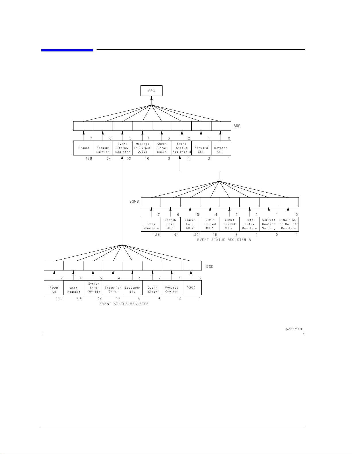
HP BASIC Programming Examples Guide

Example 4: Measurement Process Synchronization

Figure 1-2 Status Reporting Structure

Status Reporting

The analyzer has a status reporting mechanism, illustrated in Figure 1-2, that provides information about speciﬁc analyzer functions and events. The status byte is an 8-bit register with each bit summarizing the state of one aspect of the instrument. F or example , the error queue summary bit will always be set if there are any errors in the queue. The value of the status byte can be read with the HP-IB serial poll operation. This command

60 Chapter 1

HP BASIC Programming Examples Guide

Example 4: Measurement Process Synchronization

does not automatically put the instrument in remote mode, which gives you access to the analyzer front-panel functions. The status byte can also be read by sending the command OUTPSTAT. Reading the status byte does not affect its value.

The status byte summarizes the error queue, as mentioned before. It also summarizes two event-status registers that monitor speciﬁc conditions inside the instrument. The status byte also has a bit (6) that is set when the instrument is issuing a service request over HP-IB, and a bit (0) that is set in the event-status register when the analyzer has data to send out over HP-IB. See “Error Reporting,” located in the HP-IB Programming and Command Reference Guide for a discussion of the event-status registers.

Example 4A: Using the Error Queue

NOTE This program is stored as EXAMP4A on the “Programming Examples” disk

received with the network analyzer.

The error queue holds up to 20 instrument errors and warnings in the order that they occurred. Each time the analyzer detects an error condition, the analyzer displays a message, and puts the error in the error queue. If there are any errors in the queue, bit 3 of the status byte will be set. The errors can be read from the queue with the OUTPERRO command. OUTPERRO causes the analyzer to transmit the error number and message of the oldest error in the queue.

The following is an outline of the program's processing sequence:

• An I/O path is assigned for the analyzer.

• The system is initialized.

• The error-message string is allocated.

• The analyzer is released from remote control.

• The program begins an endless loop to read the error queue.

• The status byte is read with a serial poll.

• The program tests to see if an error is present in the queue.

• The error-queue bit is set.

• The program requests the content of the error queue.

• The error number and string are read.

• The error messages are printed until there are no more errors in the queue.

• The instrument is returned to local control.

• The controller emits a beep to attract the attention of the operator and resumes searching for errors.

The program is written as follows:

10 ! This program is an example of using the error queue to detect 20 ! errors generated by the analyzer. The status byte is read and 30 ! bit 3 is tested to determine if an error exists. The error queue 40 ! is printed out and emptied.

Chapter 1 61

HP BASIC Programming Examples Guide

Example 4: Measurement Process Synchronization

50 ! 60 ! EXAMP4A 70 ! 80 ASSIGN @Nwa TO 716 ! Assign an I/O path for the analyzer 90 ! 100 CLEAR SCREEN 110 ! Initialize the analyzer 120 ABORT 7 ! Generate an IFC (Interface Clear) 130 CLEAR @Nwa ! SDC (Selective Device Clear) 140 OUTPUT @Nwa;"OPC?;PRES;" ! Preset the analyzer and wait 150 ENTER @Nwa;Reply ! Read the 1 when complete 160 ! 170 DIM Error$[50] ! String for analyzer error message 180 ! 190 LOCAL @Nwa ! Release analyzer from remote control 200 ! 210 LOOP ! Endless loop to read error queue 220 REPEAT 230 Stat=SPOLL(@Nwa) ! Read status byte with serial poll 240 UNTIL BIT(Stat,3) ! Test for error queue present 250 ! 260 ! Error queue bit is set 270 REPEAT ! Loop until error number is 0 280 OUTPUT @Nwa;"OUTPERRO;" ! Request error queue contents 290 ENTER @Nwa;Err,Error$ ! Read error number and string 300 PRINT Err,Error$ ! Print error messages 310 UNTIL Err=0 ! No more errors in queue 320 ! 330 LOCAL @Nwa ! Release analyzer from remote 340 BEEP 600,.2 ! Beep to attract attention 350 END LOOP ! Repeat error search 360 ! 370 END

Running the Program

Run the program. The analyzer goes through the preset cycle. Nothing will happen at ﬁrst. The program is waiting for an error condition to activate the error queue. To cause an error, press a blank softkey. The message CAUTION: INVALID KEY will appear on the analyzer. The computer will beep and print out two error messages. The ﬁrst line will be the invalid key error message, and the second line will be the NO ERRORS message. To clear the error queue, you can either loop until the NO ERRORS message is received, or wait until the bit in the status register is cleared. In this case, we wait until the status bit in the status register is clear. Note that while the program is running, the analyzer remains in the local mode and the front-panel keys may be accessed.

The error queue will hold up to 20 errors until all the errors are read out or the instrument is preset. It is important to clear the error queue whenever errors are detected. Otherwise, old errors may be mistakenly associated with the current instrument state.

Press number of errors observed should correspond to the number of times you pressed the key.

As another example, press Cal, CORRECTION ON. A complete list of error messages and their descriptions can be found in “Error Messages” of the HP 8753E Network Analyzer User's Guide.

The program is in an inﬁnite loop waiting for errors to occur. End the program by pressing

Reset or Break on the controller keyboard.

System and then the unlabeled key several times quickly and watch the display. The

NOTE Not all messages displayed by the analyzer are put in the error queue:

operator prompts and cautions are not included.

62 Chapter 1

HP BASIC Programming Examples Guide

Example 4: Measurement Process Synchronization

Example 4B: Generating Interrupts

NOTE This program is stored as EXAMP4B on the “Programming Examples” disk

received with the network analyzer.

It is also possible to generate interrupts using the status-reporting mechanism. The status-byte bits can be enabled to generate a service request (SRQ) when set. In turn, the instrument controller can be set up to generate an interrupt on the SRQ and respond to the condition which caused the SRQ.

To generate an SRQ , a bit in the status byte is enabled using the commandSREn. A one (1) in a bit position enables that bit in the status byte. Hence, SRE 8 enables an SRQ on bit 3, the check-error queue, since the decimal value 8 equals 00001000 in binary representation. Whenever an error is put into the error queue and bit 3 is set, the SRQ line is asserted, illuminating the (S) indicator in the HP-IB status block on the front panel of the analyzer. The only way to clear the SRQ is to disable bit 3, re-enable bit 3, or read out all the errors from the queue.

A bit in the event-status register can be enabled so that it is summarized by bit 5 of the status byte. If any enabled bit in the event-status register is set, bit 5 of the status byte will also be set. For exampleESE 66 enables bits 1 and 6 of the event-status register, since in binary, the decimal number 66 equals 01000010. Hence, whenever active control is requested or a front-panel key is pressed, bit 5 of the status byte will be set. Similarly, ESNBn enables bits in event-status register B so that they will be summarized by bit 2 in the status byte.

To generate an SRQ from an event-status register, enable the desired event-status register bit. Then enable the status byte to generate an SRQ. For instance, ESE 32;SRE 32; enables the syntax-error bit. When the syntax-error bit is set, the summary bit in the status byte will be set. This will, in turn, enable an SRQ on bit 5 of the status byte, the summary bit for the event-status register.

The following is an outline of the program's processing sequence:

• An I/O path is assigned for the analyzer.

• The system is initialized.

• The status registers are cleared.

• The event-status register bit 5 is enabled.

• The status-register bit 5 is enabled.

• The interrupt pointer is enabled and points to a subroutine.

• Two bad commands are sent to the analyzer to generate errors.

• The controller reads a serial-poll byte from HP-IB in the event of an interrupt.

• The program tests for an SRQ.

• If the SRQ is not generated by the analyzer, the subroutine stops and displays SRQ FROM OTHER DEVICE.

Chapter 1 63

HP BASIC Programming Examples Guide

Example 4: Measurement Process Synchronization

• If the SRQ was generated by the analyzer, the program reads the status byte and event-status register.

• If bit 5 in the event-status register is set, the program prints: SYNTAX ERROR FROM ANALYZER.

• If bit 5 in the event-status register is NOT set, the program prints: SYNTAX ERROR BIT NOT SET.

• The SRQ interrupt is re-enabled on the bus.

• At the ﬁnish, the interrupt is deactivated.

• The analyzer is released from remote control and the program ends.

The program is written as follows:

10 ! This program is an example of using an SRQ based interrupt to 20 ! detect an error condition in the analyzer. In this example, a 30 ! syntax error is generated with an invalid command. The status byte 40 ! is read in and tested. The error queue is read, printed out and 50 ! then cleared. 60 ! 70 ! EXAMP4B 80 ! 90 ASSIGN @Nwa TO 716 ! Assign an I/O path for the analyzer 100 ! 110 CLEAR SCREEN 120 ! Initialize the analyzer 130 ABORT 7 ! Generate and IFC (Interface Clear) 140 CLEAR @Nwa ! SDC (Selective Device Clear) 150 OUTPUT @Nwa;"OPC?;PRES;" ! Preset the analyzer and wait 160 ENTER @Nwa;Reply ! Read the one from the analyzer 170 ! 180 DIM Error$[50] ! String for analyzer error message 190 ! Set up syntax error interrupt 200 OUTPUT @Nwa;"CLES;" ! Clear the status registers 210 ! 220 ! Generate SRQ when bit 5 is set 230 OUTPUT @Nwa;"ESE 32;" ! Event status register bit 5 enabled 240 ! 250 ! Generate bit 5 in status register when syntax error occurs 260 OUTPUT @Nwa;"SRE 32;" ! Status register bit 5 enabled 270 ! 280 ! Setup the interrupt pointer to a subroutine 290 ON INTR 7 GOSUB Srq_det ! When interrupt occurs go to Srq_det 300 Stat=SPOLL(@Nwa) ! Clear any pending SRQs 310 ENABLE INTR 7;2 ! Set interrupt on HP-IB bit 2 (SRQ) 320 ! 330 DISP "Waiting for bad syntax" 340 WAIT 2 ! Pause for 2 seconds 350 ! 360 OUTPUT @Nwa;"STIP 2GHZ;;" ! Send bad STOP command syntax 370 ! 380 WAIT 2 ! Pause for 2 seconds 390 DISP "" ! Clear display line 400 GOTO Finish ! Exit program example 410 ! 420 !************************** Subroutines ****************************** 430 ! 440 Srq_det: ! SRQ handler 450 Stat=SPOLL(@Nwa) ! Read serial poll byte from HP-IB 460 PRINT "Stat from Serial Poll";Stat 470 IF BIT(Stat,6) THEN ! Test for SRQ 480 PRINT "SRQ received from analyzer" 490 ELSE ! No SRQ from analyzer 500 PRINT "SRQ from other device" 510 STOP ! Stop if not from analyzer 520 END IF 530 ! 540 IF BIT(Stat,5) THEN ! Event status register bit set

64 Chapter 1

HP BASIC Programming Examples Guide

Example 4: Measurement Process Synchronization

550 PRINT "Event Status Register caused SRQ" 560 ELSE ! Some other bit set 570 PRINT "Some other bit caused the SRQ" 580 STOP ! Stop if bit not set 590 END IF 600 ! 610 REPEAT 620 OUTPUT @Nwa;"OUTPERRO;" ! Read analyzer error queue 630 ENTER @Nwa;Err,Error$ ! Read error number and string 640 PRINT Err,Error$ ! Print error message 650 UNTIL Err=0 ! No more errors in queue 660 ! 670 PRINT ! White space 680 ENABLE INTR 7;2 ! Re-enable SRQ interrupt on HP-IB 690 RETURN 700 ! 710 !************************** End Subroutines ****************************** 720 ! 730 Finish: ! End of program and exit 740 DISP "Finished" 750 OFF INTR 7 ! Turn off interrupt 760 LOCAL @Nwa ! Release HP-IB control 770 END

Running the Program

Run the program. The computer will preset the analyzer, then pause for a second or two. After pausing, the program sends an invalid command string "STIP 2 GHZ;" to cause a syntax error. This command is intended to be "STOP 2 GHZ;". The computer will display a series of messages from the SRQ-handler routine. The analyzer will display CAUTION: SYNTAX ERROR and the incorrect command, pointing to the ﬁrst character it did not understand.

The SRQ can be cleared by reading the event-status register and clearing the latched bit, or by clearing the enable registers with CLES. The syntax-error message on the analyzer display can only be cleared by the HP-IB Device Clear (DCL) message or Selected Device Clear (SDC) message. Device Clear is not commonly used because it clears every device on the bus. Selected Device Clear can be used to reset the input and output queue and the registers of a speciﬁc instrument on the bus. This will also clear all the interrupt deﬁnitions.

Chapter 1 65

HP BASIC Programming Examples Guide

Example 4: Measurement Process Synchronization

Example 4C: Power Meter Calibration

NOTE This program is stored as EXAMP4C on the “Programming Examples” disk

received with the network analyzer.

For increased accuracy of the analyzer's PORT 1-output power, a power meter calibration is available. This measurement-accuracy enhancement technique is described in “Optimizing Measurement Results” of the HP 8753E Network Analyzer User's Guide. The example described will perform the sample and sweep calibration under HP-IB remote control.

The power meter is usually connected to PORT 1 for the forward measurements. Its address must be set correctly and it must be connected to the HP-IB. The power meter address can be set by pressing: keys or the numeric key pad to complete the process. The appropriate command must be selected for the model number of power meter being used. Press model being used is displayed between the brackets.

The correction factors for the power sensor are entered into the analyzer. All of these steps are explained in the “Optimizing Measurement Results” chapter of the HP 8753E Network Analyzer User's Guide.

Local, SET ADDRESSES, ADDRESS P MTR/HPIB and using the ⇑ and ⇓

POWER MTR: [ ] until the

The number of readings-per-point must also be selected before starting. The number of points directly affects the measurement time of the calibration sequence. The power meter must be triggered and read by the analyzer for each trace point. Typically, two readings-per-point is considered appropriate. More than two readings-per-point could lead to unacceptable processing time.

To control a power meter calibration via HP-IB, the analyzer must be set to pass-control mode. The analyzer must step to the next point in the sweep and read the power present at the power meter sensor. For this operation to take place, the system controller must set up the measurement and then pass control to the analyzer to read each data point in the sweep. After reading the data point from the power meter, the analyzer passes control back to the system controller. The analyzer then sets up to measure the next point and again requests control from the system controller. This process continues until the analyzer signals that the entire sweep has been measured point-by-point.

The following is an outline of the program's processing sequence:

• An I/O path is assigned for the analyzer.

• The system is initialized.

• The number of points in the trace is set.

• The number of readings-per-point is set.

• The frequency span is set.

NOTE The frequency span of this example program must be modiﬁed in order

to correspond to the frequency ranges of the HP 8753E.

• The reference channel is measured.

66 Chapter 1

HP BASIC Programming Examples Guide

Example 4: Measurement Process Synchronization

• The power meter calibration array is allocated.

• The power meter model is chosen.

• The status registers are cleared.

• The request-control summary bit is enabled.

• The pass-control mode is enabled.

• A calibration sweep is taken to begin the sequence.

• The status byte is read until control is requested.

• The computer passes control to the analyzer.

• The display is cleared and the analyzer is set to talker/listener mode.

• The HP-IB interface status is read until control is returned.

• The program loops until all the points have been measured.

• The power meter calibration is enabled.

• The calibration data is output to the controller in FORM 4, ASCII format.

• The power meter-calibration factors are read into the controller.

• The analyzer is released from remote control and the program ends. The program is written as follows:

10 ! This routine does a power meter cal using pass control. 20 ! A measurement cycle takes place on each point of the trace. The 30 ! point is measured by the power meter and the measured value read 40 ! into the analyzer. The command TAKCS; arms this measurement mode. 50 ! The number of measurements is determined by the number of points in 60 ! the trace, the number of readings per point and an extra measurement 70 ! cycle to release the powr meter. 80 ! Control is passed to the analyzer, the point is measured and 90 ! the data is transferred to the analyzer. Control is passed back to 100 ! the controller and the cycle begins again. Serial poll is used to 110 ! read the status byte of the analyzer and test the logic. 120 ! The HP-IB interface status register is monitored to determine when 130 ! control is returned to the interface from the analyzer. 140 ! 150 ! EXAMP4C 160 ! 170 ASSIGN @Nwa TO 716 ! Assign an I/O path for the analyzer 180 ! 190 CLEAR SCREEN 200 ! Initialize the analyzer 210 ABORT 7 ! Generate an IFC (Interface Clear) 220 CLEAR @Nwa ! SDC (Selective Device Clear) 230 OUTPUT @Nwa;"OPC?;PRES;" ! Preset the analyzer and wait 240 ENTER @Nwa;Reply ! Read the 1 when complete 250 ! 260 INTEGER Stat 270 ! 280 ! Set up the analyzer parameters 290 Numpoints=11 ! Number of points in the trace 300 Numreads=2 ! Number of readings per point 310 Startf=1.00E+8 ! Start frequency 320 Stopf=5.0E+8 ! Stop frequency 330 ! 340 OUTPUT @Nwa;"POIN";Numpoints;";" ! Set trace length to numpoints 350 OUTPUT @Nwa;"NUMR";Numreads;";" ! Set number of readings per point 360 OUTPUT @Nwa;"STAR";Startf ! Set start frequency 370 OUTPUT @Nwa;"STOP";Stopf ! Set stop frequency

Chapter 1 67

HP BASIC Programming Examples Guide

Example 4: Measurement Process Synchronization

380 OUTPUT @Nwa;"MEASR;" ! Measure the reference channel 390 ! 400 ALLOCATE Pmcal(1:Numpoints) ! Create power meter cal array 410 ! 420 ! Store the original trace for comparison 430 OUTPUT @Nwa;"DATI;" 440 OUTPUT @Nwa;"DISPDATM;" 450 OUTPUT @Nwa;"AUTO;" 460 ! 470 ! Select the power meter being used for cal 480 ! OUTPUT @Nwa;"POWM ON;" ! Select 436A power meter 490 OUTPUT @Nwa;"POWMOFF;DEBUON;" ! Select 437B/438A power meter 500 ! 510 ! Set analyzer HP-IB, status regs to interrupt on pass control 520 OUTPUT @Nwa;"CLES;" ! Clear status registers 530 OUTPUT @Nwa;"ESE2;" ! Enable request control summary bit 540 OUTPUT @Nwa;"SRE32;" ! SRQ on events status register 550 ! 560 PRINT "Beginning Power Meter CAL" 570 OUTPUT @Nwa;"USEPASC;" ! Enable pass control operation 580 OUTPUT @Nwa;"TAKCS;" ! Take Cal Sweep 590 ! 600 FOR I=1 TO Numpoints*Numreads+1 ! Points * Number of readings plus 1 610 ! Serial poll does not place analyzer in remote operation 620 ! and does not require the analyzer to process the command. 630 ! 640 REPEAT ! Repeat until SRQ detected 650 Stat=SPOLL(@Nwa) ! Serial poll to read status byte 660 DISP "Stat ";Stat;" Waiting for request" 670 UNTIL BIT(Stat,6) ! SRQ detected for request control 680 OUTPUT @Nwa;"ESR?;" ! Read status register to clear 690 ENTER @Nwa;Reply ! Read and discard register value 700 ! 710 PRINT "Passing Control" ! status read and pasing control 720 PASS CONTROL @Nwa ! Pass control to analyzer 730 ! 740 REPEAT 750 ! Read HP-IB interface state information register. 760 STATUS 7,6;Hpib ! Test HP-IB register for control 770 ! 780 ! Reading the interface status register does not interact with the 790 ! analyzer. Bit 6 is set when control is returned. 800 ! 810 DISP "Waiting for control" 820 UNTIL BIT(Hpib,6) ! Loop until control is returned 830 NEXT I 840 ! 850 PRINT "Finished with Power meter Cal" 860 DISP "" ! Clear display message 870 ! 880 OUTPUT @Nwa;"TALKLIST;" ! Restore Talker/Listener operation 890 OUTPUT @Nwa;"CLES;" ! Clear and reset status byte operation 900 ! 910 OUTPUT @Nwa;"PWMCONES;" ! Power meter cal correct one sweep 920 OUTPUT @Nwa;"OPC?;WAIT;" ! Wait for the analyzer to finish 930 ENTER @Nwa;Reply ! Read the 1 when complete 940 ! 950 ! Read the power meter cal correction factors 960 OUTPUT @Nwa;"FORM4;" ! ASCII data format to read cal data 970 OUTPUT @Nwa;"OUTPPMCAL1;" ! Request the power meter cal factors 980 ENTER @Nwa;Pmcal(*) ! Read the factors 990 ! 1000! Display the power meter cal factors 1010 PRINT "Point","Factor" 1020 FOR I=1 TO Numpoints ! Cycle throught the factors 1030 PRINT I,Pmcal(I) 1040 NEXT I 1050! 1060 LOCAL @Nwa ! Release HP-IB control 1070 END

68 Chapter 1

HP BASIC Programming Examples Guide

Example 4: Measurement Process Synchronization

Running the Program

The analyzer is preset and the power meter-calibration routine begins. The analyzer displays the message "WAITING FOR HP-IB CONTROL"' when it is requesting control. The system controller display prints "Passing Control" when control is passed to the analyzer. The controller displays "Waiting for request" while the analyzer has control and is reading the power meter.

The interaction of the messages and the movement of the cursor allow observation of the calibration process. Once the calibration is complete, the analyzer displays"POWER METER

CAL IS COMPLETE" and the system controller displays "Finished with Power meter Cal".

The power meter-calibration mode (with one sweep of correction data) is enabled and the calibration is switched ON. At the completion of the program, talker/listener mode is restored, the event-status registers are cleared (to halt the status-byte interaction), the power meter correction factors are displayed, the sweep is placed in continuous-sweep mode, the analyzer is released from HP-IB control, and the program ends.

Chapter 1 69

HP BASIC Programming Examples Guide

Example 5: Network Analyzer System Setups

Saving and Recalling Instrument States

NOTE The most efﬁcient option for storing and recalling analyzer states is

using the analyzer's internal registers to save the CAL data. Recalling these registers is the fastest solution to restoring analyzer setups. See “Printing, Plotting, or Saving Measurement Results” in the HP 8753E Network Analyzer User's Guide for detailed information on the analyzer's internal storage registers.

In the event that all the registers have been used, the internal disk drive is not used, or if internal memory limitations exist, then these external solutions become viable.

The purpose of this example is to demonstrate several programming options for storing and recalling entire instrument states over HP-IB. The examples describe two different processes for storing and recalling instrument states. The ﬁrst example accomplishes the task using the learn string. The second example involves reading both the learn string and the calibration arrays out of the analyzer and storing them to disk or storing them in the system controller itself.

Using the learn string is a very rapid way of saving the instrument state, but using direct disk access has the advantage of automatically storing calibrations, cal kits, and data along with the instrument state.

A complete analyzer setup requires sending the learn string and a calibration array to set the analyzer parameters. The CAL array may also be placed in the analyzer, just as if a calibration was performed. By sending both sets of data, the analyzer may be quickly setup for a measurement.

Several different measurements may be required in the course of testing a device. An efﬁcient way of performing multiple measurements is to send both the calibration array and the learn string, and then perform the measurements.

Example 5A: Using the Learn String

NOTE This program is stored as EXAMP5A on the “Programming Examples” disk

received with the network analyzer.

The learn string is a very fast and easy way to read an instrument state. The learn string includes all front-panel settings, the limit table for each channel, and the list-frequency table. It can be read out of the analyzer with the command OUTPLEAS, and input to the analyzer with the command INPULEAS.

The following is an outline of the program's processing sequence:

• An I/O path is assigned for the analyzer.

70 Chapter 1

HP BASIC Programming Examples Guide

Example 5: Network Analyzer System Setups

• The system is initialized.

• The string storage is allocated.

• The learn string is requested.

• The string is read without any processing.

• The analyzer is released from remote control.

• The instrument state is changed by the operator.

• The learn string is sent back to the analyzer.

• The analyzer is released from remote control and the program ends. The program is written as follows:

1 ! This program shows how to retrieve a learn string from the analyzer 2 ! into a string array. The state of the analyzer is then changed and the 3 ! learn string re-loaded to return the analyzer to the previous settings. 4 ! 5 ! EXAMP5A 6 ! 7 OPTION BASE 1 8 ASSIGN @Nwa TO 716 ! Assign an I/O path for the analyzer 9 ASSIGN @Nwa_bin TO 716;FORMAT OFF 10 ! 11 CLEAR SCREEN 12 ! Initialize the analyzer 13 ABORT 7 ! Generate an IFC (Interface Clear) 14 CLEAR @Nwa ! SDC (Selected Device Clear) 15 ! 16 INTEGER Header,Length ! 2-byte header and length of string 17 ! 18 OUTPUT @Nwa;”OUTPLEAS;” ! Output the learn string 19 ENTER @Nwa_bin;Header,Length ! Read header and length first 20 ! 21 ALLOCATE INTEGER State(Length/2) ! Integer array to contain the string 22 ! 23 ENTER @Nwa_bin;State(*) ! Read the string 24 LOCAL @Nwa ! Release HP-IB control 25 ! 26 INPUT “Change state and press ENTER”,A$ 27 ! 28 OUTPUT @Nwa;”INPULEAS;” ! Send the learnstring to analyzer 29 OUTPUT @Nwa_bin;Header,Length,State(*) 30 DISP “Analyzer state has been restored!” 31 ! 32 OUTPUT @Nwa;”OPC?;WAIT;” ! Wait for the analzyer to finish 33 ENTER @Nwa;Reply ! Read the 1 when complete 34 LOCAL @Nwa ! Release HP-IB control 35 END

Running the Program

Run the program. When the program stops, change the instrument state and press Enter on the controller. The analyzer will be returned to its original state by using the learn string.

Chapter 1 71

HP BASIC Programming Examples Guide

Example 5: Network Analyzer System Setups

Example 5B: Reading Calibration Data

NOTE This program is stored as EXAMP5B on the “Programming Examples” disk

received with the network analyzer.

This example demonstrates:

• how to read measurement calibration data out of the network analyzer

• how to read it back into the analyzer

• how to determine which calibration is active

The data used to perform measurement-error correction is stored inside the analyzer in one (or more) of twelve calibration-coefﬁcient arrays. Each array is a speciﬁc error coefﬁcient, and is stored and transmitted as an error-corrected data array. Each point is a real/imaginary pair, and the number of points in the array is the same as the number of points in the sweep. The ﬁve data formats also apply to the transfer of calibration-coefﬁcient arrays. “Printing , Plotting, and Saving Measurement Results” in the HP 8753E Network Analyzer User's Guide contains information on the storage locations for calibration coefﬁcients and different calibration types.

A computer can read out the error coefﬁcients using the commands OUTPCALC01, OUTPCALC02,…through OUTPCALC12. Each calibration type uses only as many arrays as required, beginning with array 1. Hence, it is necessary to know the type of calibration about to be read out. Attempting to read an array not being used in the current calibration causes the "REQUESTED DATA NOT CURRENTLY AVAILABLE" warning.

A computer can also store calibration coefﬁcients in the analyzer. To do this, declare the type of calibration data about to be stored in the analyzer just as if you were about to perform that calibration. Then, instead of calling up different classes, transfer the calibration coefﬁcients using the INPUCALCnn; commands. The variables nn are a data pair appended to the command representing a calibration number from 01 through 12. When all the coefﬁcients are stored in the analyzer, activate the calibration by issuing the mnemonic SAVC;, and trigger a sweep on the analyzer.

This example reads the calibration coefﬁcients into a very large array, from which they can be examined, modiﬁed, stored, or put back into the instrument. If the data is to be directly stored onto disk, it is usually more efﬁcient to use FORM 1 (analyzer's internal-binary format), and to store each coefﬁcient array as it is read in.

The following is an outline of the program's processing sequence:

• An I/O path is assigned for the analyzer.

• A binary path is assigned.

• The system is initialized.

• The calibration types and number of arrays are deﬁned.

• The integer variables for reading the headers are deﬁned.

• The calibration type and number of arrays are read by the controller.

• The output is formatted in FORM 3.

72 Chapter 1

HP BASIC Programming Examples Guide

Example 5: Network Analyzer System Setups

• The number of points in the trace is read.

• The memory is allocated for the calibration arrays.

• Each calibration array is requested from the analyzer.

• Header information is read with a binary I/O path.

• The elements from each calibration array are read in.

• The next calibration array is requested until all the arrays have been read.

• The calibration type is sent to the analyzer.

• Each calibration array is sent.

• The calibration is activated.

• The analyzer is released from remote control and the program ends. The program is written as follows:

10 ! This program shows how to manipulate calibration data from the analyzer. 20 ! It demonstrates how to read calibration data from the analyzer, and 30 ! how to replace it. The type of calibration active is determined and 40 ! the program reads in the correct number of arrays. The number of points 50 ! in the trace, and in the cal array, is determined and used to dimension 60 ! storage arrays. 70 ! 80 ! EXAMP5B 90 ! 100 ASSIGN @Nwa TO 716 ! Assign an I/O path for the analyzer 110 ASSIGN @Nwa_bin TO 716;FORMAT OFF ! Assign binary path 120 ! 130 CLEAR SCREEN 140 ! Initialize the analyzer 150 ABORT 7 ! Generate an IFC (Interface Clear) 160 CLEAR @Nwa ! SDC (Selected Device Clear) 170 ! 180 ! Data for determining CAL type and number of arrays 190 DATA "CALIRESP",1,"CALIRAI",2,"CALIS111",3 200 DATA "CALIS221",3,"CALIFUL2",12 210 DATA "NOOP",0 220 ! 230 INTEGER Hdr,Lgth,I,J ! Integers for reading headers 240 ! 250 READ Calt$,Numb ! Read CAL type from data statement 260 IF Numb=0 THEN GOTO 690 ! If no CAL type is present Exit 270 OUTPUT @Nwa;Calt$;"?;" ! Query if CAL type is active 280 ENTER @Nwa;Active ! Read 1 if active 290 IF NOT Active THEN GOTO 250 ! Load another CAL type and re-try 300 ! 310 PRINT Calt$,Numb ! Active CAL and number of arrays 320 ! 330 OUTPUT @Nwa;"FORM3;" ! Form 3 IEEE 64 bit floating point 340 OUTPUT @Nwa;"POIN?;" ! Request trace length 350 ENTER @Nwa;Poin ! Read number of points 360 ALLOCATE Cal(1:Numb,1:Poin,1:2) ! Arrays for CAL arrays 370 ! Number of arrays, number of points real and imag value per point 380 ! 390 FOR I=1 TO Numb ! Read arrays 400 OUTPUT @Nwa USING "K,ZZ";"OUTPCALC",I ! Format I to add 0 in command 410 ENTER @Nwa_bin;Hdr,Lgth ! Read header & length from array 420 FOR J=1 TO Poin ! Read elements for CAL array 430 ENTER @Nwa_bin;Cal(I,J,1),Cal(I,J,2) ! Read real & imag pair elements 440 NEXT J ! Next location in array 450 NEXT I ! Next CAL array 460 ! 470 ! All CAL arrays have been read 480 ! 490 INPUT "PRESS RETURN TO RE-TRANSMIT CALIBRATION",Dum$

Chapter 1 73

HP BASIC Programming Examples Guide

Example 5: Network Analyzer System Setups

500 ! 510 OUTPUT @Nwa;"FORM3;" ! Use same format as read 520 OUTPUT @Nwa;Calt$;";" ! Send CAL type to analyzer 530 ! 540 FOR I=1 TO Numb ! Send each array in CAL 550 DISP "TRANSMITTING ARRAY: ",I ! Show array number 560 OUTPUT @Nwa USING "K,ZZ";"INPUCALC",I ! Send array number 0 format 570 OUTPUT @Nwa_bin;Hdr,Lgth ! Send header & array length 580 FOR J=1 TO Poin ! Send each array element 590 OUTPUT @Nwa_bin;Cal(I,J,1),Cal(I,J,2) ! Real and Imag pair 600 NEXT J ! Next element in array 610 NEXT I ! Next array 620 ! 630 OUTPUT @Nwa;"SAVC;" ! Activate CAL 640 ! 650 OUTPUT @Nwa;"CONT;" ! Restore continuous sweep 660 OUTPUT @Nwa;"OPC?;WAIT;" ! Wait for analyzer to finish 670 ENTER @Nwa;Reply ! Read the 1 when complete 680 ! 690 DISP "Finished with CAL transfer" 700 LOCAL @Nwa ! Release HP-IB control 710 END

Running the Program

Before executing the program, perform a calibration. The program is able to detect which type of calibration is active. With that information, it

predicts how many arrays to read out. When all the arrays have been sent to the computer, the program prompts the user. The operator then turns the calibration OFF or performs a completely different calibration on the analyzer and continues the program. The computer reloads the old calibration. The operator should not preset the analyzer because the instrument settings must be the same as those that were present when the calibration was taken.

NOTE The re-transmitted calibration is associated with the current

instrument state: the instrument has no way of knowing the original state associated with the calibration data. For this reason, it is recommended that the learn string be used to store the instrument state whenever calibration data is stored. The next example demonstrates how to reload the analyzer state with both the learn string and the calibration arrays.

74 Chapter 1

HP BASIC Programming Examples Guide

Example 5: Network Analyzer System Setups

Example 5C: Saving and Restoring the Analyzer Instrument State

NOTE This program is stored as EXAMP5C on the “Programming Examples” disk

received with the network analyzer.

NOTE The instrument state may also be stored in the analyzer's internal

registers. This is the fastest and most efﬁcient method for toggling between instrument states. This example is for use when the analyzer's internal memory is full, or when the are other internal-memory limitations.

This example demonstrates how to use both the learn string and the calibration arrays to completely re-program the analyzer state. If you were performing two entirely different measurements on a device and wanted to quickly change between instrument states and perform the measurements, this example program is a potential solution.

The example will request the learn string and calibration array from the analyzer and store them in a disk ﬁle on the system controller. Once the storage is complete, the operator will be prompted to change the state of the analyzer and then re-load the state that was previously stored in the disk ﬁle. Once the ﬁle is created on the disk, the state information can be retrieved from the controller and restored on the analyzer.

NOTE The disk ﬁle can only be created once. Errors will occur if the operator

repeatedly tries to re-create the ﬁle.

For this example, only a thru calibration will be performed and transferred. This means only one calibration array will be read from the analyzer and written to the disk ﬁle with the instrument state. To work with more elaborate calibrations, additional arrays will need to be deﬁned and transferred to the disk ﬁle. This is not difﬁcult, but requires some further programming steps which were omitted in the interest of presenting a simple example.

The following is an outline of the program's processing sequence:

• An I/O path is assigned for the analyzer.

• A binary path is assigned.

• The integers for reading the headers are deﬁned.

• The system is initialized.

• An array is created to hold the learn string.

• The learn string is requested by the controller.

• The number of points in the trace is read.

• The controller allocates an array for the calibration data.

• The calibration data is read into the controller.

Chapter 1 75

HP BASIC Programming Examples Guide

Example 5: Network Analyzer System Setups

• The controller creates and assigns a data ﬁle for the calibration array and the learn string.

• The learn string and calibration array are stored in the disk ﬁle.

• The operator presses

Enter on the controller to read the calibration data back into the

analyzer.

• The learn string is read from the disk ﬁle and output to the analyzer.

• The calibration array is read in from the disk ﬁle and stored in the analyzer.

• The analyzer is returned to continuous-sweep mode.

• The analyzer is released from remote control and the program ends.

The program is written as follows:

10 ! This program reads an instrument state and stores it in a disk file. 20 ! The learn string and CAL array are both read into the controller and 30 ! then transferred to a disk file for storage. The file contents are 40 ! then restored to the analyzer. The analyzer is preset to the default 50 ! settings before the instrument state is transferred back. 60 ! 70 ! EXAMP5C 80 ! 90 ASSIGN @Nwa TO 716 ! Assign an I/O path for the analyzer 100 ASSIGN @Nwa_bin TO 716;FORMAT OFF ! Assign a binary path 110 ! 120 INTEGER Head,Length ! Integer 2 byte format for headers 130 ! 140 CLEAR SCREEN 150 ! Initialize the analyzer 160 ABORT 7 ! Generate an IFC (Interface Clear) 170 CLEAR @Nwa ! SDC (Selected Device Clear) 180 ! 190 ! Read in the learn string as a form 1 binary data trace 200 DIM Learn$[3000] ! Array to hold learn string 210 ! 220 OUTPUT @Nwa;"OPC?;SING;" ! Place analyzer in single sweep 230 ENTER @Nwa;Reply ! Read the 1 when complete 240 ! 250 OUTPUT @Nwa;"OUTPLEAS;" ! Request learn string 260 ENTER @Nwa USING "+,-K";Learn$ 270 ! 280 ! Allocate an array for storing the CAL data 290 OUTPUT @Nwa;"POIN?;" ! Find number of points in trace 300 ENTER @Nwa;Num_points ! Read number to allocate array 310 ALLOCATE Cal_array(1:Num_points,1:2) ! Real and Imag for each point 320 ! 330 ! Read Cal array 340 OUTPUT @Nwa;"FORM3;" ! Form 3 64 bit floating point data 350 OUTPUT @Nwa;"OUTPCALC01;" ! Request the cal array 360 ! 370 ! Read the #A and 2 byte length as integers 380 ENTER @Nwa_bin;Head,Length,Cal_array(*) ! Read cal array data 390 ! 400 ! Write instrument state data to disk file 410 ! CREATE BDAT "DATA_FILE:,1406",1,Length+3000 ! Create data file once! 420 ASSIGN @File TO "DATA_FILE:,1406 " ! Assign I/O path to file 430 OUTPUT @File;Learn$ ! Send learn string to disk file 440 OUTPUT @File;Head,Length,Cal_array(*) ! Send CAL arrays to disk file 450 ASSIGN @File TO * ! Close file 460 ! 470 INPUT "Cal data received. Press ENTER to send it back.",A$ 480 ! 490 ! Read arrays from file 500 ! 510 DIM Learn2$[3000] ! String for learn string storage 520 ASSIGN @File TO "DATA_FILE:,1406" ! Open file for reading arrays 530 ENTER @File;Learn2$ ! Read learn string from file

76 Chapter 1

HP BASIC Programming Examples Guide

Example 5: Network Analyzer System Setups

540 ! 550 ENTER @File;Head,Length ! Read CAL data headers from file 560 Size=Length/16 ! Array is 2 numbers, 8 bytes per number 570 ALLOCATE Cal_array2(1:Size,1:2) ! new cal array from file record 580 ENTER @File;Cal_array2(*) ! Read cal array from disk file 590 ! 600 ! Send Learn string back 610 OUTPUT @Nwa;"INPULEAS;",Learn2$ ! Send learn string array 620 ! 630 ! Send Cal array back 640 OUTPUT @Nwa;"CALIRESP;" ! Send CAL type (Response) 650 OUTPUT @Nwa;"INPUCALC01;" ! Output CAL array to analyzer 660 OUTPUT @Nwa_bin;Head,Length,Cal_array2(*) 670 OUTPUT @Nwa;"OPC?;SAVC;" ! Save the CAL array 680 ENTER @Nwa;Reply ! Read the 1 when complete 690 ! 700 OUTPUT @Nwa;";CONT;" ! Start the analzyer sweeping 710 OUTPUT @Nwa;"OPC?;WAIT;" ! Wait for the analyzer to finish 720 ENTER @Nwa;Reply 730 LOCAL @Nwa ! Release HP-IB control 740 END

Running the Program

Setup the analyzer and perform a thorough calibration. Run the program. The program prompts the operator to change the state of the analyzer

and then press Enter to continue. At this point, the analyzer state is stored on the disk ﬁle in the controller. Pressing within the controller and then on to the analyzer.

Enter will begin the transfer from the disk ﬁle to internal arrays

Once completed:

• The original state will be restored.

• The analyzer will be sweeping.

• The analyzer will be calibrated.

• COR will be displayed on the analyzer's display.

Chapter 1 77

HP BASIC Programming Examples Guide

Example 6: List-Frequency Tables and Limit-Test Tables

Using List Frequency Sweep Mode

The analyzer normally takes data points spaced at regular intervals across the overall frequency range of the measurement. For example, for a 2 GHz frequency span using 201 points, data will be taken at intervals of 10 MHz. The list frequency sweep mode allows the operator to select the speciﬁc points, or frequency spacing between points, at which measurements are to be made. This mode of operation allows ﬂexibility in setting up tests that insure device performance. By only sampling speciﬁc points, measurement time is reduced. List frequency sweeps are also discussed in “ Application and Operation Concepts” of the HP 8753E Network Analyzer User's Guide.

The following three example programs illustrate the use of the analyzer's list frequency sweep mode to perform arbitrary frequency testing. Examples 6A1 (Stepped List Mode) and 6A2 (Swept List Mode) allow the operator to construct a table of list frequency segments which is then loaded into the analyzer's list frequency table. There are a maximum of 30 segments available. Each segment stipulates a start and stop frequency, and the number of data points to be taken over that frequency range. In Example 6A2 (Swept List Mode), each segment also stipulates a power value and IF bandwidth. List frequency segments can be overlapped in the stepped list mode but not in the swept list mode. The total number of points in all the segments must not exceed 1632.

Examples 6A1 (Stepped List Mode) and 6A2 (Swept List Mode) take advantage of the computer's capabilities to simplify creating and editing a list frequency table. The table is entered and completely edited before being transmitted to the analyzer. To simplify the programming task, options such as entering center frequency, frequency span, or step size are not included.

Example 6B lets the operator select a speciﬁc segment to “zoom-in.” A single instrument can be programmed to measure several different devices, each with its own frequency range, using a single calibration. When a speciﬁc device is connected, the operator selects the appropriate segment for that device.

The command sequence for entering a list frequency table imitates the key sequence followed when entering a table from the front panel: there is a command for every key-press. Editing a segment is also the same as the front-panel key sequence, but the analyzer automatically reorders each edited segment in order of increasing start frequency.

The list frequency information may be acquired using the limit-test results array. The actual stimulus points are available as the ﬁrst element in the array.

The list frequency table is also carried as part of the learn string. While the table cannot be modiﬁed as part of the learn string, it can be stored and recalled with very little effort by storing and recalling the learn string. See programming example 5A “Using the Learn String,” and the “Data Processing Chain” in the HP-IB Programming and Command Reference Guide for details on using learn strings.

78 Chapter 1

HP BASIC Programming Examples Guide

Example 6: List-Frequency Tables and Limit-Test Tables

Example 6A1: Setting Up a List Frequency Table In Stepped List Mode

NOTE This program is stored as EXAMP6A1 on the “Programming Examples” disk

received with the network analyzer.

The purpose of this example is to show how to create a list frequency table in stepped list mode and then transmit the table to the analyzer.

In the stepped list mode, the source steps to the next frequency point where it stops long enough for the analyzer to take data. For electrically long devices, this mode ensures that the measurement will not be impacted by IF delay. In addition, this mode provides the most ﬂexibility in specifying the list of frequencies.

The following is an outline of the program's processing sequence:

• An I/O path is assigned for the analyzer.

• The system is initialized.

• The existing list frequencies are edited and cleared.

• The number of segments to deﬁne is read in.

• An array for the list segments is deﬁned.

• The parameters for each segment are requested.

• If the operator wants to edit, the segment parameters are re-entered.

• The new list is sent to the analyzer.

• The analyzer is released from remote control and the program ends. The program is written as follows:

1 ! This program shows how to enter and edit a list frequency table. 2 ! Any existing table is deleted and a new table is defined and 3 ! edited. This list is then sent to the analyzer. Any number of 4 ! segments or points may be entered. Be sure not to enter more than 5 ! 1632 points or 30 segments. 6 ! 7 ! EXAMP6A1 8 ! 9 ASSIGN @Nwa TO 716 ! Assign an I/O path for the analyzer 10 ! 11 CLEAR SCREEN 12 ! Initialize the analyzer 13 ABORT 7 ! Generate an IFC (Interface Clear) 14 CLEAR @Nwa ! SDC (Selective Device Clear) 15 OUTPUT @Nwa;”OPC?;PRES;” ! Preset the analyzer and wait 16 ENTER @Nwa;Reply ! Read the 1 when complete 17 ! 18 ! Edit the list frequency table and set its type 19 ! LISTTYPE = LSTP (stepped list mode) 20 ! 21 OUTPUT @Nwa;”EDITLIST;LISTTYPELSTP;” 22 ! 23 OUTPUT @Nwa;”CLEL;” ! Clear the existing list frequencies 24 ! 25 INPUT “Number of segments?”,Numb ! Read number of segments to define 26 ALLOCATE Table(1:Numb,1:3) ! Define an array for the list segments 27 ! 28 PRINT USING “10A,15A,15A,20A”;”SEGMENT”,”START(MHZ)”,”STOP(MHZ)”,”NUMBER OF POINTS”

Chapter 1 79

HP BASIC Programming Examples Guide

Example 6: List-Frequency Tables and Limit-Test Tables

29 ! 30 FOR I=1 TO Numb ! Cycle through the segments and read in the values 31 GOSUB Loadpoin 32 NEXT I 33 ! 34 LOOP 35 INPUT “DO YOU WANT TO EDIT? Y OR N”,An$ 36 EXIT IF An$=”N” 37 INPUT “ENTRY NUMBER?”,I ! Get an entry number 38 GOSUB Loadpoin ! Go load point 39 END LOOP 40 ! 41 OUTPUT @Nwa;”EDITLIST” ! Send the new list to the analyzer 42 FOR I=1 TO Numb ! Send one segment at a time 43 OUTPUT @Nwa;”SADD;” ! Add a segment 44 OUTPUT @Nwa;”STAR”;Table(I,1);”MHZ;” ! Start frequency 45 OUTPUT @Nwa;”STOP”;Table(I,2);”MHZ;” ! Stop frequency 46 OUTPUT @Nwa;”POIN”,Table(I,3),”;” ! Number of points 47 OUTPUT @Nwa;”SDON;” ! Segment done 48 NEXT I ! Next segment to send to the analyzer 49 ! 50 OUTPUT @Nwa;”EDITDONE;” ! Done with list 51 OUTPUT @Nwa;”LISFREQ;” ! Set list frequency mode 52 ! 53 OUTPUT @Nwa;”OPC?;WAIT;” ! Wait for analyzer to finish 54 ENTER @Nwa;Reply ! Read the 1 when complete 55 LOCAL @Nwa ! Release HP-IB control 56 STOP ! End of main program 57 ! 58 ! ***************************Subroutines ****************************** 59 ! 60 Loadpoin: ! Sub to read in each segment value 61 INPUT “START FREQUENCY? (MHZ)”,Table(I,1) ! Read start frequency 62 INPUT “STOP FREQUENCY? (MHZ)”,Table(I,2) ! Read stop frequency 63 INPUT “NUMBER OF POINTS?”,Table(I,3) ! Read number of points in seg 64 IF Table(I,3)=1 THEN Table(I,2)=Table(I,1) ! Single point same start stop 65 ! 66 ! Print new segment into table on display 67 PRINT TABXY(0,I+1);I;TAB(10);Table(I,1);TAB(25); 68 PRINT Table(I,2);TAB(40),Table(I,3) 69 RETURN 70 END

Running the Program

The program displays the frequency list table as it is entered. During editing, the displayed table is updated as each line is edited. The table is not re-ordered. At the completion of editing, the table is entered into the analyzer, and list frequency sweep mode is switched ON. During editing, pressing

Enter leaves an entry at the old value.

The start frequency, stop frequency, and number of points for the last segment entered may be observed on the analyzer's display.

Activate a marker and select the discrete-marker mode to observe the point spacing. Use an exaggerated scale with just a few points to ﬁnd the list-frequency spacing between points.

Example 6A2: Setting Up a List Frequency Table In Swept List Mode

NOTE This program is stored as EXAMP6A2 on the “Programming Examples” disk

received with the network analyzer.

The purpose of this example is to show how to create two tables: a list frequency table in swept list mode, and a limit-test table. Both tables are then transmitted to the analyzer.

80 Chapter 1

HP BASIC Programming Examples Guide

Example 6: List-Frequency Tables and Limit-Test Tables

In the swept list mode, the source sweeps through each segment, with the analyzer taking data during the sweep. This can increase throughput by up to 6 times over a stepped sweep. In addition, this mode expands the list table to include a power value and IF bandwidth for each deﬁned segment. The only restriction is that you cannot specify segments with overlapping frequencies. F or more information on the swept list mode , refer to the HP 8753E Network Analyzer User's Guide.

The following is an outline of the program's processing sequence:

• An array for the type of limit line is deﬁned and initialized.

• An array for the list table (frequency list and limit lines) is deﬁned and initialized with data.

• An I/O path is assigned for the analyzer.

• The system is initialized.

• A variable is initialized with the number of segments in the list table.

• The analyzer is placed into hold mode and the port powers are uncoupled for the active channel.

• The existing list frequencies are edited and the analyzer swept list mode is selected.

• The analyzer is instructed to set the IF bandwidth and power for each port according to the values from the list table.

• The new frequency list table is sent to the analyzer.

• The sweep mode is set to list frequency mode and S21 measurement. A single sweep is taken.

• The analyzer display is autoscaled.

• The existing limit lines are edited and cleared.

• The new limit table is sent to the analyzer.

• The limit lines and limit test are turned on.

• The analyzer is released from remote control and the program ends.

The program is written as follows:

1 ! This program creates a swept list table for a specific filter measurement. 2 ! The program first builds a list frequency table from a hardcoded set of 3 ! list segments. It then builds a limit table based on the same hardcoded 4 ! data. When modifying the table data below, make sure that no two segments 5 ! overlap in frequency. 6 ! 7 ! EXAMP6A2 8 ! 9 !-----------------------------------------------------------------10 ! The following constants are used to represent limit line “type” 11 ! in the table below. 12 ! 13 No_limit=0 14 ! 15 ! 1 = flat line 16 ! 2 = sloped line 17 ! 3 = single point (also used to terminate a line segment) 18 !-----------------------------------------------------------------19 !

Chapter 1 81

HP BASIC Programming Examples Guide

Example 6: List-Frequency Tables and Limit-Test Tables

20 DIM Limtype$(1:3)[2] 21 DATA FL, SL, SP 22 READ Limtype$(*) 23 ! 24 ! The list below has the following entries: 25 ! Start: start frequency 26 ! Stop: Segment stop 27 ! Pts: Segment number of points 28 ! P1: Power at port 1 29 ! P2: Power at port 2 30 ! IFBW: Segment IFBW 31 ! upper: Upper Limit 32 ! lower: Lower Limit 33 ! strt type: Limit Line type for start of segment 34 ! end type: Limit Line type for end of segment 35 !-----------------------------------------------------------------36 DIM Listtable(1:6,1:10) 37 Freqlist: ! |strt|end 38 ! List: Start | Stop | Pts | P1 | P2 | IFBW | uppr | lower |type|type 39 ! ----------------------------------------------------------------------40 ! ----------------------------------------------------------------------41 DATA 570.000, 588.000, 5, 10, 0, 10, -90, -200, 1, 0 42 DATA 588.000, 598.000, 11, 0, 0, 100, -85, -200, 1, 3 43 DATA 600.000, 664.000, 15, -10, -10, 3700, 0, 0, 0, 0 44 DATA 664.000, 678.000, 100, -10, -10, 3700, 0, -6, 1, 3 45 DATA 678.000, 768.000, 10, -10, -10, 1000, 0, 0, 0, 0 46 DATA 768.000, 768.000, 1, 10, 0, 10, -90, -200, 3, 3 47 ! ----------------------------------------------------------------------48 READ Listtable(*) 49 ! 50 ASSIGN @Nwa TO 716 ! Assign an I/O path for the analyzer 51 ! 52 CLEAR SCREEN 53 ! Initialize the system 54 ABORT 7 55 CLEAR @Nwa 56 OUTPUT @Nwa;”OPC?;PRES;” 57 ENTER @Nwa;Done 58 Numb=SIZE(Listtable,1) ! Number of segments in list table 59 OUTPUT @Nwa;”HOLD;” ! Hold mode allows faster set up 60 OUTPUT @Nwa;”PORTPUNCPLD;” ! Uncouple ports 61 ! 62 ! Create the list frequency table from the table above 63 ! LISTTYPE = LSWP (swept list mode) 64 ! 65 OUTPUT @Nwa;”EDITLIST;LISTTYPELSWP;” 66 ! 67 ! Turn on list power mode for each port (uncoupled) 68 ! Turn on list ifbw mode 69 ! 70 OUTPUT @Nwa;”LISIFBWMON;” ! IF bandwidth set by list 71 OUTPUT @Nwa;”S21;LISPWRMON;” ! Port 1 power set by list 72 OUTPUT @Nwa;”S22;LISPWRMON;” ! Port 2 power set by list 73 ! 74 FOR I=1 TO Numb 75 OUTPUT @Nwa;”SADD;STAR”;Listtable(I,1);”MHZ;” 76 OUTPUT @Nwa;”STOP”;Listtable(I,2);”MHZ;” 77 OUTPUT @Nwa;”POIN”;Listtable(I,3);”;” 78 OUTPUT @Nwa;”S11;” ! Port 1 active 79 OUTPUT @Nwa;”SEGPOWER”;Listtable(I,4),”;” 80 OUTPUT @Nwa;”S22;” ! Port 2 active 81 OUTPUT @Nwa;”SEGPOWER”;Listtable(I,5),”;” 82 OUTPUT @Nwa;”SEGIFBW”;Listtable(I,6),”;” 83 OUTPUT @Nwa;”SDON;” 84 NEXT I 85 OUTPUT @Nwa;”EDITDONE;” 86 OUTPUT @Nwa;”LISFREQ;S21;OPC?;SING;” 87 ENTER @Nwa;Done 88 OUTPUT @Nwa;”AUTOSCAL;WAIT;” 89 ! 90 ! Now create the corresponding limit table 91 ! 92 OUTPUT @Nwa;”EDITLIML;CLEAL;” ! Initiate the limit table 93 FOR I=1 TO Numb 94 IF Listtable(I,9)<>No_limit THEN

82 Chapter 1

HP BASIC Programming Examples Guide

Example 6: List-Frequency Tables and Limit-Test Tables

95 OUTPUT @Nwa;”SADD” ! Add a new limit segment 96 OUTPUT @Nwa;”;LIMS”;Listtable(I,1);”MHZ” 97 OUTPUT @Nwa;”;LIMU”;Listtable(I,7) 98 OUTPUT @Nwa;”;LIML”;Listtable(I,8) 99 OUTPUT @Nwa;”;LIMT”;Limtype$(Listtable(I,9)) 100 OUTPUT @Nwa;”;SDON;” 101 IF Listtable(I,10)<>No_limit THEN ! 102 OUTPUT @Nwa;”SADD “ ! Add a new limit segment 103 OUTPUT @Nwa;”;LIMS”;Listtable(I,2);”MHZ” 104 OUTPUT @Nwa;”;LIMT”;Limtype$(Listtable(I,10)) 105 OUTPUT @Nwa;”;SDON;” 106 END IF 107 END IF 108 NEXT I 109 OUTPUT @Nwa;”EDITDONE;LIMILINEon;LIMITESTon;” 110 ! 111 LOCAL @Nwa 112 END

Running the Program

The program requires no input from the operator. The list frequency table data and limit-test table data is read directly from the program code into the array. Next, the analyzer is set up to respond to the IF bandwidth and port power parameters of the list frequency table. After the list frequency data is entered into the analyzer, the list frequency sweep mode is initiated and a single sweep is taken. Lastly, the limit-test table data is entered into the analyzer and the limit lines and limit test are activated.

The analyzer should now indicate whether the measurement trace passes or fails the limit test.

Chapter 1 83

HP BASIC Programming Examples Guide

Example 6: List-Frequency Tables and Limit-Test Tables

Example 6B: Selecting a Single Segment from a Table of Segments

NOTE This program is stored as EXAMP6B on the “Programming Examples” disk

received with the network analyzer.

This example program demonstrates how to deﬁne a single segment as the operating-frequency range of the analyzer from a table of segments stored in the controller . The program assumes that a list frequency table has already been entered into the analyzer, either manually, or using the program in Example 6A1 or Example 6A2.

The program ﬁrst loads the list frequency table into the computer by reading the start and stop frequencies of each segment and the number of points for each segment. The segment's parameters are then displayed on the computer screen, and the operator can choose which segment is to be used by the analyzer. Note that only one segment can be chosen at a time.

The following is an outline of the program's processing sequence:

• An I/O path is assigned for the analyzer.

• The system is initialized.

• The list frequency segment is edited.

• The largest segment number is set.

• The highest segment number is requested.

• The number of actual segments is read in.

• A list frequency table is deﬁned and the segments are read in to the controller from the analyzer.

• The operator selects one of the segments of the sweep.

• The controller “zooms-in” and sweeps the deﬁned segment.

• The operator ends the program by entering segment number

• The analyzer returns to sweeping all the segments in the table.

• The activation loop is ended and the program ends.

The program is written as follows:

10 ! This program shows how to select a single segment from a list 20 ! frequency sweep and activate it as the sweep. The list frequency 30 ! table is read from the analyzer and displayed on the computer 40 ! screen. The operator is prompted to select a segment and the 50 ! program then activates it. All the segments are activated upon 60 ! completion. 70 ! 80 ! EXAMP6B 90 ! 100 ASSIGN @Nwa TO 716 ! Assign an I/O path for the analyzer 110 ! 120 CLEAR SCREEN 130 ! Initialize the analyzer 140 ABORT 7 ! Generate an IFC (Interface Clear) 150 CLEAR @Nwa ! SDC (Selected Device Clear)

84 Chapter 1

HP BASIC Programming Examples Guide

Example 6: List-Frequency Tables and Limit-Test Tables

160 ! 170 ! Print header for table of existing segments 180 PRINT USING "10A,15A,15A,20A";"SEGMENT","START(MHZ)","STOP(MHZ)","NUMBER OF

POINTS" 190 OUTPUT @Nwa;"EDITLIST;" ! Edit list frequency segment 200 OUTPUT @Nwa;"SEDI30;" ! Set largest segment number 210 OUTPUT @Nwa;"SEDI?;" ! Request number of highest segment 220 ENTER @Nwa;Numsegs ! Read number of actual segments 230 ! 240 ! Setup table and read segments from analyzer 250 ALLOCATE Table(1:Numsegs,1:3) ! Allocate table of segments 260 FOR I=1 TO Numsegs ! Cycle through segments 270 GOSUB Readlist ! Read in segment definitions 280 NEXT I ! Next segment 290 ! 300 ! Loop and read segment to be activated 310 LOOP ! Request operator to enter segment 320 INPUT "SELECT SEGMENT NUMBER: (0 TO EXIT)",Segment 330 EXIT IF Segment=0 ! Exit point 340 OUTPUT @Nwa;"EDITDONE;";"SSEG";Segment;";" ! Set active segment to sweep 350 END LOOP ! End activation loop 360 ! 370 OUTPUT @Nwa;"ASEG;" ! Set all segment sweep 380 DISP "PROGRAM ENDED" 390 ! 400 OUTPUT @Nwa;"OPC?;WAIT;" ! Wait for analyzer to finish 410 ENTER @Nwa;Reply ! Read the 1 when complete 420 LOCAL @Nwa ! Release HP-IB control 430 STOP ! End of main program 440 ! 450 ! ************************** Subroutines ******************************* 460 ! 470 Readlist: ! Read segment list from analyzer 480 OUTPUT @Nwa;"EDITLIST;" ! Edit segment list 490 OUTPUT @Nwa;"SEDI",I,";" ! Select segment to edit 500 OUTPUT @Nwa;"STAR;" ! Send start freq to display value 510 OUTPUT @Nwa;"OUTPACTI;" ! Output active function value 520 ENTER @Nwa;Table(I,1) ! Read start frequency 530 OUTPUT @Nwa;"STOP;" ! Send stop freq to display value 540 OUTPUT @Nwa;"OUTPACTI;" ! Output active function value 550 ENTER @Nwa;Table(I,2) ! Read stop frequency 560 OUTPUT @Nwa;"POIN;" ! Send number of points to display 570 OUTPUT @Nwa;"OUTPACTI;" ! Output active function value 580 ENTER @Nwa;Table(I,3) ! Read number of points 590 ! 600 IF I=18 THEN ! Pause if more than 17 segments 610 INPUT "PRESS RETURN FOR MORE",A$ ! Read Return to continue 620 END IF 630 ! Print new header for segment data 640 IMAGE 4D,6X,4D.6D,3X,4D.6D,3X,4D ! Format image to disp segment data 650 PRINT USING 640;I;Table(I,1)/1.E+6;Table(I,2)/1.E+6;Table(I,3) 660 RETURN 670 ! 680 END

Running the Program

The program will read the parameters for each list-frequency segment from the analyzer, and build a table containing all the segments. The parameters of each segment will be printed on the computer screen. If there are more than 17 segments, the program will pause. Press read is 30 (the maximum number of segments the analyzer can hold). Use the computer's

Page Up and Page Down keys to scroll through the list of segments if there are more than 17.

After all the segments are displayed, the program will prompt the operator for a speciﬁc segment to be used. Type in the number of the segment, and the analyzer will then “zoom-in” on that segment. The program will continue looping, allowing continuous

Chapter 1 85

Return to see more segments. The maximum number of segments that can be

HP BASIC Programming Examples Guide

Example 6: List-Frequency Tables and Limit-Test Tables

selection of different segments. To exit the loop, type 0. This will restore all the segments (with the command ASEG), allowing the analyzer to sweep all of the segments, and the program will terminate.

Using Limit Lines to Perform PASS/FAIL Tests

There are two steps to performing limit testing on the analyzer via HP-IB. First, limit speciﬁcations must be deﬁned and loaded into the analyzer. Second, the limits are activated, the device is measured, and its performance to the speciﬁed limits is signaled by a pass or fail message on the analyzer's display.

Example 6C illustrates the ﬁrst step, setting up limits. Example 6D performs the actual limit testing.

86 Chapter 1

HP BASIC Programming Examples Guide

Example 6: List-Frequency Tables and Limit-Test Tables

Example 6C: Setting Up a Limit-Test Table

NOTE This program is stored as EXAMP6C on the “Programming Examples” disk

received with the network analyzer.

The purpose of this example is to show how to create a limit-test table and transmit it to the analyzer.

The command sequence for entering a limit-test table imitates the key sequence followed when entering a table from the analyzer's front panel: there is a command for every key-press. Editing a limit line is also the same as the key sequence, but remember that the analyzer automatically re-orders the table in order of increasing start frequency.

The limit-test table is also carried as part of the learn string. While it cannot be modiﬁed as part of the learn string, the learn string can be stored and recalled with very little effort. See “Data-Processing Chain” in Example 5A and the HP-IB Programming and Command Reference Guide for details on using learn strings.

This example takes advantage of the computer's capabilities to simplify creating and editing the table. The table is entered and completely edited before being transmitted to the analyzer. To simplify the programming task, options such as entering offsets are not included.

This example automates the front-panel operation of entering a limit-test table. Front-panel operation and limits are discussed in the “Application and Operation Concepts” in the HP 8753E Network Analyzer User's Guide.

The following is an outline of the program's processing sequence:

• An I/O path is assigned for the analyzer.

• The system is initialized.

• The limit lines are edited and cleared.

• The number of limits is requested.

• The limit table is created.

• The string array of limit types is created.

• The operator is prompted to enter the new limit values.

• The new limit table is sent back to the analyzer.

• The limit line is activated.

• The limit test is activated.

• The analyzer is returned to local control and the program ends. The program is written as follows:

10 ! This program shows how to create a limit table and send it to the 20 ! analyzer. The operator enters the desired limits when prompted for 30 ! the stimulus value, upper and lower value and type of limit 40 ! desired. Once the table is created, the limits are sent to the 50 ! analyzer and activated. 60 !

Chapter 1 87

HP BASIC Programming Examples Guide

Example 6: List-Frequency Tables and Limit-Test Tables

70 ! EXAMP6C 80 ! 90 ASSIGN @Nwa TO 716 ! Assign an I/O path for the analyzer 100 ! 110 CLEAR SCREEN 120 ! Initialize the analyzer 130 ABORT 7 ! Generate an IFC (Interface clear) 140 CLEAR @Nwa ! SDC (Selected Device Clear) 150 OUTPUT @Nwa;"OPC?;PRES;" ! Preset the analyzer and wait 160 ENTER @Nwa;Reply ! Read the 1 when completed 170 ! 180 OUTPUT @Nwa;"EDITLIML;" ! Edit limit lines 190 OUTPUT @Nwa;"CLEL;" ! Clear any existing limits 200 INPUT "NUMBER OF LIMITS?",Numb ! Request the number of limits 210 ALLOCATE Table(1:Numb,1:3) ! Create a table 220 ALLOCATE Limtype$(Numb)[2] ! Create string array of limit types 230 ! 240 ! Print out the header for the table 250 PRINT USING "10A,20A,15A,20A";"SEG","STIMULUS (MHz)","UPPER (dB)","

LOWER (dB)", "TYPE" 260 ! 270 ! Prompt the operator to enter the limit values 280 FOR I=1 TO Numb ! Cycle through the limits 290 GOSUB Loadlimit ! Go read limit values 300 NEXT I ! Next limit value 310 ! 320 ! Allow the operator to edit the array entered 330 LOOP ! Cycle to edit limit lines 340 INPUT "DO YOU WANT TO EDIT? Y OR N",An$ 350 EXIT IF An$="N" ! Exit loop on N and send to analyzer 360 INPUT "ENTRY NUMBER?",I ! Read limit number to edit 370 GOSUB Loadlimit ! Go read limit values 380 END LOOP ! Next edit entry 390 ! 400 ! Send the limit line array segments to the analyzer 410 OUTPUT @Nwa;"EDITLIML;" ! Edit the limit 420 FOR I=1 TO Numb ! Each segment of the limit 430 OUTPUT @Nwa;"SADD;" ! Add segment 440 OUTPUT @Nwa;"LIMS";Table(I,1);"MHZ" ! Send segment stimulus value 450 OUTPUT @Nwa;"LIMU";Table(I,2);"DB" ! Upper limit value 460 OUTPUT @Nwa;"LIML";Table(I,3);"DB" ! Lower limit value 470 IF Limtype$(I)="FL" THEN OUTPUT @Nwa;"LIMTFL;" ! Flat limit 480 IF Limtype$(I)="SL" THEN OUTPUT @Nwa;"LIMTSL;" ! Sloping limit 490 IF Limtype$(I)="SP" THEN OUTPUT @Nwa;"LIMTSP;" ! Point limit 500 OUTPUT @Nwa;"SDON;" ! Segment done 510 NEXT I ! next segment 520 ! 530 OUTPUT @Nwa;"EDITDONE;" ! Edit complete 540 OUTPUT @Nwa;"LIMILINEON;" ! Turn limit line on 550 OUTPUT @Nwa;"LIMITESTON;" ! Turn limit test on 560 ! 570 OUTPUT @Nwa;"OPC?;WAIT;" ! Wait for the analyzer to finish 580 ENTER @Nwa;Reply ! Read the 1 when complete 590 ! 600 LOCAL @Nwa ! Release HP-IB control 610 STOP ! End of main program 620 ! 630 !************************** Subroutines ****************************** 640 ! 650 Loadlimit: ! Sub to interact to load data 660 INPUT "STIMULUS VALUE? (MHz)",Table(I,1) ! and print table created 670 INPUT "UPPER LIMIT VALUE? (DB)",Table(I,2) 680 INPUT "LOWER LIMIT VALUE? (DB)",Table(I,3) 690 INPUT "LIMIT TYPE? (FL=FLAT, SL=SLOPED, SP=SINGLE POINT)",Limtype$(I) 700 ! 710 ! Format and display table values 720 PRINT TABXY(0,I+1);I;TAB(10);Table(I,1);TAB(30);Table(I,2);TAB(45),

Table(I,3),TAB(67);Limtype$(I) 730 RETURN ! Next limit value 740 ! 750 END

88 Chapter 1

HP BASIC Programming Examples Guide

Example 6: List-Frequency Tables and Limit-Test Tables

Running the Program

CAUTION This example program will delete any existing limit lines before

entering the new limits. If this is not desired, omit the line(s) that clear the existing limits (in this case, the command "CLEL;" contained in LINE 190). This program begins by presetting the analyzer. The programmer will have to add the necessary command lines to set the analyzer to the operating conditions required for testing. The example program will show the limit lines deﬁned, but the limits will always fail without additional analyzer setup.

The program displays the limit table as it is entered. During editing, the displayed table is updated as each line is edited. The table is not reordered. At the completion of editing, the table is entered into the analyzer, and limit-testing mode switched ON. The analyzer will rearrange the table in ascending order starting with the lowest start frequency entry. During editing, simply pressing

Enter leaves an entry at the old value.

Chapter 1 89

HP BASIC Programming Examples Guide

Example 6: List-Frequency Tables and Limit-Test Tables

Example 6D: Performing PASS/FAIL Tests While Tuning

NOTE This program is stored as EXAMP6D on the “Programming Examples” disk

received with the network analyzer.

The purpose of this example is to demonstrate the use of the limit/search-fail bits in event-status register B, to determine whether a device passes the speciﬁed limits. Limits can be entered manually, or using the Example 6C.

The limit/search-fail bits are set and latched when limit testing or a marker search fails. There are four bits, one for each channel for both limit testing and marker search. See Figure 1-2 “Status Reporting Structure” and Table 1-4 “Units as a Function of Display Format” in theHP 8753E Network Analyzer HPIB Programming and Command Reference Guide for additional information. Their purpose is to allow the computer to determine whether the test/search executed was successful. They are used in the following sequence:

1. Clear event-status register B.

2. Trigger the limit test or marker search.

3. Check the appropriate fail bit. When using limit testing, the best way to trigger the limit test is to trigger a single sweep.

By the time the single sweep command (SING) ﬁnishes, limit testing will have occurred. NOTE If the device is tuned during the sweep, it may be tuned into and then

out of limit, causing a limit test to qualify as “passed” when the device is not in fact within the speciﬁed limits.

When using marker searches (max, min, target, and widths), outputting marker or bandwidth values automatically triggers any related searches. Therefore, all that is required is to check the fail bit after reading the data.

In this example, several consecutive sweeps must qualify as “passing” in order to insure that the limit-test pass was not extraneous due to the device settling or operator tuning during the sweep. Upon running the program, the number of “passed” sweeps for qualiﬁcation is entered. For very slow sweeps, a small number of sweeps such as two are appropriate. For relatively fast sweeps, where the device requires time to settle after tuning, as many as six or more sweeps may be more appropriate.

The following is an outline of the program's processing sequence:

• An I/O path is assigned for the analyzer.

• The system is initialized.

• The pass counter is initialized on entry.

• The analyzer takes a sweep.

• The event-status register B byte is output and the channel-1 limit is tested.

• If the device fails the ﬁrst sweep, the operator is prompted to insure it is tuned correctly

and the device is measured again.

90 Chapter 1

HP BASIC Programming Examples Guide

Example 6: List-Frequency Tables and Limit-Test Tables

• If the device passes the ﬁrst sweep, the operator is prompted not to touch the device as testing continues.

• If the device passes the required number of sweeps, the operator is prompted that the device has passed and to connect the next device for testing.

• The program initializes the pass counter and begins to measure the new device.

The program is written as follows:

10 ! This program demonstrates Pass/Fail tests using limit lines. The 20 ! program uses the latch-on-fail limit bits in event status register 30 ! B to determine if the device performance passes the specified test 40 ! limit lines. It then requires that the device passes for multiple 50 ! consecutive sweeps in order to ensure that the device is static in 60 ! the response and not varying. The operator specifies how many sweeps 70 ! are required to pass the test. 80 ! 90 ! EXAMP6D 100 ! 110 ASSIGN @Nwa TO 716 ! Assign an I/O path for the analyzer 120 ! 130 CLEAR SCREEN 140 ! Initialize the analyzer No preset to retain settings for testing 150 ABORT 7 ! Generate an IFC (Interface Clear) 160 CLEAR @Nwa ! SDC (Selected Device Clear) 170 ! 180 INPUT "Number of consecutive passed sweeps for qualification?",Qual 190 Pass=0 ! Initialize pass counter on entry 200 ! 210 Tune: DISP "TUNE DEVICE AS NECESSARY" ! Device is not passing warning 220 ! 230 Measure:OUTPUT @Nwa;"OPC?;SING;" ! Single sweep and wait 240 ENTER @Nwa;Reply ! Read the 1 when completed 250 ! 260 OUTPUT @Nwa;"ESB?;" ! Event status register B byte 270 ENTER @Nwa;Estat ! Reading byte clears the register 280 ! 290 IF BIT(Estat,4) THEN ! Bit 4 is failed limit on channel 1 300 IF Pass>0 THEN BEEP 1200,.05 ! passed before? Now not passing beep 310 Pass=0 ! Reset pass to 0 320 GOTO Tune ! Adjust and measure again 330 END IF 340 ! 350 BEEP 2500,.01 ! Limit test passed passing beep 360 Pass=Pass+1 ! Increment number of passes 370 DISP "LEAVE DEVICE ALONE" ! Warn not to adjust as it passed 380 ! 390 IF Pass<Qual THEN GOTO Measure ! If not enough passes to qualify 400 ! 410 ! Device passed 420 DISP "DEVICE PASSED!" ! Number of passes enough to qualify 430 FOR I=1 TO 10 ! Announce the device passed and 440 BEEP 1000,.05 ! prompt operator to connect new 450 BEEP 2000,.01 ! device to test. 460 NEXT I 470 ! 480 INPUT "PRESS RETURN FOR NEXT DEVICE",Dum$ 490 Pass=0 ! Initialize pass counter 500 GOTO Measure ! Begin measurement 510 ! 520 END

Running the Program

NOTE This program assumes a response calibration (through calibration) or a

full 2-port calibration has been performed prior to running the program.

Chapter 1 91

HP BASIC Programming Examples Guide

Example 6: List-Frequency Tables and Limit-Test Tables

Set up a limit-test table on channel 1 for a speciﬁc device either manually, or using the program in Example 6C.

Run the program, and enter the number of passed sweeps desired for qualiﬁcation. After entering the qualiﬁcation number, connect the device. When a sweep passes, the computer beeps. When enough consecutive sweeps qualify the device as “passing,” the computer emits a dual-tone beep to attract the attention of the operator, and then prompts for a new device.

To test the program's pass/fail accuracy, try causing the DUT to fail by loosening the cables connecting the DUT to the analyzer and running the program again.

92 Chapter 1

HP BASIC Programming Examples Guide

Example 7: Report Generation

The analyzer has three operating modes with respect to HP-IB. These modes can be changed by accessing softkeys in the computer is present. This mode allows the analyzer to control the system. The other two modes allow a remote system controller to coordinate certain actions: in talker/listener mode the remote system controller can control the analyzer, as well as coordinate plotting and printing; and in pass-control mode the remote system controller can pass active control to the analyzer so that the analyzer can plot, print, control a power meter, or load/store to disk. The amount of peripheral interaction is the main difference between talker/listener and pass-control mode.

Example 7A1: Operation Using Talker/Listener Mode

NOTE This program is stored as EXAMP7A1 on the “Programming Examples” disk

received with the network analyzer.

Local menu. System-controller mode is used when no

The commands OUTPPLOT and OUTPPRIN allow talker/listener mode plotting and printing via a one way data path from the analyzer to the plotter or printer. The computer sets up the path by addressing the analyzer to talk, the plotter to listen, and then releasing control of the analyzer in order to transfer the data. The analyzer will then make the plot or print. When it is ﬁnished, it asserts the End or Identify (EOI) control line on HP-IB. The controller detects the presence of EOI and re-asserts control of the HP-IB . This example program makes a plot using the talker/listener mode.

NOTE One of the attributes of the OUTPPLOT command is that the plot can

include the current softkey menu. The plotting of the softkeys is enabled with the PSOFTON; command and disabled with the PSOFTOFF; command.

The following is an outline of the program's processing sequence:

• An I/O path is assigned for the analyzer.

• The system is initialized.

• The selected frequency span is swept once.

• The plot command is sent to the analyzer.

• The analyzer is set to talker mode and the plotter is set to listener mode.

• The plot is spooled to the plotter.

• The analyzer is set to listener mode when the controller detects an EOI from the analyzer.

• The controller puts the analyzer back in continuous-sweep mode.

• The analyzer is returned to local control and the program ends.

The program is written as follows:

Chapter 1 93

HP BASIC Programming Examples Guide

Example 7: Report Generation

10 ! This example shows a plot operation under the control of the 20 ! analyzer. The analyzer is commanded to output plot data, the 30 ! plotter is addressed to listen, and the analyzer to talk. The 40 ! controller watches for EOI at the end of the plot sequence and 50 ! then regains control of the HP-IB operations. 60 ! 70 ! EXAMP7A1 80 ! 90 ASSIGN @Nwa TO 716 ! Assign an I/O path for the analyzer 100 ! 110 CLEAR SCREEN 120 ! Initialize analzyer without preset to preserve data 130 ABORT 7 ! Generate an IFC ( Interface Clear) 140 CLEAR @Nwa ! SDC (Selected Device Clear) 150 ! 160 OUTPUT @Nwa;"OPC?;SING;" ! Stop sweep and prepare for plot 170 ENTER @Nwa;Reply ! Read in "1" when completed 180 ! 190 OUTPUT @Nwa;"OUTPPLOT;" ! Send plot command 200 SEND 7;UNL LISTEN 5 TALK 16 DATA ! Unlisten address devices and plot 210 DISP "Plotting and waiting for EOI" 220 WAIT .5 ! Pause 500 mS to start process 230 ! 240 REPEAT ! Loop until EOI detected bit is set 250 STATUS 7,7;Stat ! Read HP-IB interface register 7 260 UNTIL BIT(Stat,11) ! Test bit 11 EOI on HP-IB 270 ! 280 End_plot:DISP "End of plot" 290 ! 300 OUTPUT @Nwa;"CONT;" ! Restore continuous sweep 310 OUTPUT @Nwa;"OPC?;WAIT;" ! Wait for analyzer to finish 320 ENTER @Nwa;Reply ! Read the 1 when complete 330 LOCAL @Nwa ! Release remote control 340 END

Running the Program

The analyzer will go into remote, and make the plot. During the plot, the computer will display the message Plotting and waiting for EOI. When the plot is completed, the analyzer asserts the EOI line on the HP-IB. The computer detects this and displays the End of plot message.

If a problem arises with the plotter, such as no pen or paper , the analyzer cannot detect the situation because it only has a one-way path of communication. Hence, the analyzer will attempt to continue plotting until the operator intervenes and aborts the plot by pressing the analyzer's

Pressing

• Aborts the plot.

• Causes the warning message CAUTION: PLOT ABORTED.

• Asserts EOI to return control of the bus to the system controller. Because of possible peripheral malfunctions, it is generally advisable to use pass-control

mode, which allows two way communication between the peripherals and the analyzer.

Local key.

Local will do the following:

94 Chapter 1

HP BASIC Programming Examples Guide

Example 7: Report Generation

Example 7A2: Controlling Peripherals Using Pass-Control Mode

NOTE This program is stored as EXAMP7A2 on the “Programming Examples” disk

received with the network analyzer.

If the analyzer is in pass-control mode and it receives a command telling it to plot, print, control a power meter, or store/load to disk, it sets bit 1 in the event-status register to indicate that it requires control of the bus. If the computer then uses the HP-IB pass-control command to pass control to the analyzer, the analyzer will take control of the bus and access the peripheral. When the analyzer no longer requires control, it will pass control back to the computer.

In this example, the pass-control mode is used to allow the network analyzer to dump a screen display to a printer.

Pass-control mode allows the analyzer to control the printer while sending the screen display to be printed. The analyzer requests control from the instrument controller and the controller allows the analyzer to take control of the HP-IB and dump the plot. The instrument controller must not interact with the HP-IB while this remote analyzer control is taking place. Once the printer-dump operation is complete, the analyzer passes control back to the controller and the controller continues programming the analyzer.

NOTE The analyzer assumes that the address of the computer is correctly

stored in its HP-IB addresses menu under

CONTROLLER. If this address is incorrect, control will not return to the

Local, SET ADDRESSES, ADDRESS:

computer. Similarly, if control is passed to the analyzer while it is in talker/listener mode, control will not return to the computer.

Control should not be passed to the analyzer before it has set event-status-register bit 1 making it Request Active Control. If the analyzer receives control before the bit is set, control is passed immediately back to the controller.

When the analyzer becomes the active system controller , it is free to address devices to talk and listen as required. The only functions denied the analyzer are the ability to assert the interface clear line (IFC), and the remote line (REN). These are reserved for the master system controller. As the active system controller, the analyzer can send and receive messages from printers, plotters, and disk drives.

The following is an outline of the program's processing sequence:

• An I/O path is assigned for the analyzer.

• The system is initialized.

• The status registers are cleared.

• Bit 1 of ESR request control is set.

• The ESR interrupt for SRQ is enabled.

• The pass-control mode is enabled.

• The data is dumped to the printer.

Chapter 1 95

HP BASIC Programming Examples Guide

Example 7: Report Generation

• The program loops until the SRQ bit is set.

• The status byte is read with a serial poll.

• The program tests for bit 6, SRQ.

• If SRQ is detected, the program tests for pass control (bit 5 of the status byte).

• If the analyzer requests control, the system controller gives the analyzer control of the bus.

• The program loops and waits for the analyzer to complete the print dump.

• The analyzer reads the interface.

• If bit 6 is active in the controller, control is returned from the analyzer to the controller.

• The status-byte assignments are cleared.

• The analyzer returns to continuous-sweep mode.

• The analyzer is returned to local control and the program ends.

The program is written as follows:

10 ! This example shows a pass-control operation to print the display 20 ! under the analyzer HP-IB control. The controller reads the status 30 ! of the analyzer looking for SRQ to indicate that the analyzer is 40 ! requesting control. Once control is passed to the analyzer, the 50 ! controller monitors the status of its interface registers to detect 60 ! when the interface is again the active controller. The analyzer will 70 ! pass control back to the controller when finished. 80 ! 90 ! EXAMP7A2 100 ! 110 ASSIGN @Nwa TO 716 ! Assign an I/O path for the analyzer 120 ! 130 CLEAR SCREEN 140 ! Initialize the analyzer without preset to preserve data 150 ABORT 7 ! Generate an IFC ( Interface Clear) 160 CLEAR @Nwa ! SDC (Selected Device Clear) 170 ! 180 OUTPUT @Nwa;"OPC?;SING;" ! Single sweep and stop for print 190 ENTER @Nwa;Reply ! Read in "1" when complete 200 ! 210 OUTPUT @Nwa;"CLES;" ! Clear status registers 220 OUTPUT @Nwa;"ESE2;" ! Enable bit 1 of ESR request control 230 OUTPUT @Nwa;"SRE32;" ! Enable ESR interrupt for SRQ 240 ! 250 OUTPUT @Nwa;"USEPASC;" ! Enable pass control mode 260 OUTPUT @Nwa;"PRINALL;" ! Begin printer dump 270 ! 280 REPEAT ! Loop until SRQ bit is set 290 Stat=SPOLL(@Nwa) ! Read status byte with serial poll 300 UNTIL BIT(Stat,6) ! Test for bit 6, SRQ 310 ! 320 Pass_control: ! SRQ detected. Test for pass control 330 IF BIT(Stat,5) THEN ! Requested pass control 340 PASS CONTROL @Nwa ! Send take control message 350 ELSE ! Not bit 5, some other event 360 DISP "SRQ but not request pass control" 370 STOP ! Halt program 380 END IF 390 ! 400 DISP "Printing from analyzer and waiting for control" 410 ! 420 REPEAT ! Loop and wait for completion 430 STATUS 7,6;Hpib ! Read HP-IB interface register 440 UNTIL BIT(Hpib,6) ! Bit 6 is active controller 450 !

96 Chapter 1

HP BASIC Programming Examples Guide

Example 7: Report Generation

460 DISP "Control returned from analyzer" 470 OUTPUT @Nwa;"TALKLIST;" ! Set talker/listener mode again 480 OUTPUT @Nwa;"CLES;" ! Clear status byte assignments 490 ! 500 OUTPUT @Nwa;"CONT;" ! Start analyzer sweeping again 510 OUTPUT @Nwa;"OPC?;WAIT;" ! Wait for analyzer to finish 520 ENTER @Nwa;Reply ! Read the 1 when complete 530 ! 540 LOCAL @Nwa ! Release HP-IB control 550 END

Running the Program

The analyzer will brieﬂy ﬂash the message WAITING FOR CONTROL, before actually receiving control and generating the printer output. The computer will display the Printing from analyzer and waiting for control message.

When the printer output is complete, the analyzer passes control back to the address stored as the controller address under the detect the return of active control and exit the wait loop. The controller will display the message Control returned from analyzer and then release the analyzer from remote control.

NOTE Because the program waits for the analyzer's request for control, it can

be used to respond to front-panel requests as well. Remove the "PRINALL;" command from the program and run the program. Nothing will happen until the operator requests a print, plot, or disk access from the front panel of the analyzer. For example, press

Copy, and PRINT MONOCHROME.

Local, SET ADDRESSES menu. The computer will

Local,

Chapter 1 97

HP BASIC Programming Examples Guide

Example 7: Report Generation

Example 7A3: Printing with the Serial Port

NOTE This program is stored as EXAMP7A3 on the “Programming Examples” disk

received with the network analyzer.

This program will select the serial port and program the analyzer to copy its display to a printer. There are a number of commands associated with the serial and parallel ports which allow the programmer to conﬁgure output modes such as the baud rate and the handshake type used by the port and the printer. In this example, the serial port is conﬁgured by the program. The interface may also be conﬁgured from the analyzer's front-panel keys by pressing selection of the serial-interface parameters.

Since the HP-IB port is not being used for the copy operation, programming of the analyzer and measurement operations may continue once the copy operation has been initiated. An internal spooler in the analyzer's memory provides buffering of the printer operation. In the example which follows, the status byte of the analyzer is checked to determine when the print operation is complete.

• An I/O path is assigned to the analyzer.

Local, SET ADDRESSES, PRINTER PORT. This menu allows manual

• The analyzer is initialized.

• A single sweep is taken and the analyzer is placed in hold mode.

• The status registers are cleared.

• The copy-complete bit is set and enabled.

• The printer operation and communication modes are set.

• The print command is sent.

• The analyzer is released from remote control and placed in continuous-sweep mode.

• The analyzer is polled until the status bit representing copy complete is detected.

• The analyzer is released from remote control and the program ends.

The program is written as follows:

10 ! This program shows how to set up and print the display through the 20 ! serial printer port. 30 ! 40 ! EXAMP7A3 50 ! 60 ASSIGN @Nwa TO 716 ! Assign an I/O path for the analyzer 70 ! 80 CLEAR SCREEN 90 ! Initialize the analzyer without preset to preserve the data 100 ABORT 7 ! Generate an IFC (Interface Clear) 110 CLEAR @Nwa ! SDC (Selected Device Clear) 120 ! 130 OUTPUT @Nwa;"OPC?;SING;" ! Single sweep and stop for print 140 ENTER @Nwa;Reply ! Read the 1 when complete 150 ! 160 OUTPUT @Nwa;"CLES;" ! Clear status registers 170 OUTPUT @Nwa;"ESNB128;" ! Enable copy complete 180 OUTPUT @Nwa;"SRE4;" ! Enable Event Status Register B 190 OUTPUT @Nwa;"PRNTRAUTF OFF;" ! Set printer auto feed off 200 OUTPUT @Nwa;"PRNTYPTJ;" ! Select ThinkJet printer 210 OUTPUT @Nwa;"PRNPRTSERI;" ! Select serial port for output

98 Chapter 1

HP BASIC Programming Examples Guide

Example 7: Report Generation

220 OUTPUT @Nwa;"PRNTRBAUD 9600;" ! Set baud rate to 9600 bps 230 OUTPUT @Nwa;"PRNHNDSHK XON;" ! Use Xon-Xoff handshake 240 ! 250 OUTPUT @Nwa;"PRINALL;" ! Print screen 260 ! 270 DISP "PRINTING" 280 ! 290 ! Set up next measurement over HP-IB 300 OUTPUT @Nwa;"CONT;" ! Restore continuous sweep 310 ! 320 ! Measurements can continue but wait for print to finish 330 REPEAT ! Test for bit 2 (4) ESRB 340 Stat=SPOLL(@Nwa) 350 UNTIL BIT(Stat,2) ! Wait for printer to complete 360 ! 370 DISP "DONE" 380 LOCAL @Nwa ! Release HP-IB control 390 END

Running the Program

Run the program. The analyzer is initialized, set to single-sweep mode, and a sweep is taken. The program sets the system up to print the analyzer's display to an HP ThinkJet printer connected to the interface. At this time, the analyzer can continue making measurements as the ThinkJet prints the display. When the analyzer display has ﬁnished printing, the controller displays the message:"DONE", the analyzer is released from HP-IB control, and the program ends.

Chapter 1 99

HP BASIC Programming Examples Guide

Example 7: Report Generation

Example 7B1: Plotting to a File and Transferring the File Data to a Plotter

NOTE This program is stored as EXAMP7B1 on the “Programming Examples” disk

received with the network analyzer.

Another report-generation technique is to transfer the plotter string to a disk ﬁle, and retrieve and plot the disk ﬁle at another time. T est time is increased when a hardcopy plot occurs during the measurement process. It may be more convenient to plot the data at another site or time. One solution to this problem is to capture the plot data using the controller and store it to a disk ﬁle. This disk ﬁle may then be read from the controller and the contents transferred to a plotter. This next example shows a method of accomplishing this task.

The analyzer is initialized without presetting the analyzer. The data that is in place on the analyzer is not disturbed by the program operation. A large string is dimensioned to hold the plotter commands as they are received from the analyzer. The length of this string depends upon the complexity of the analyzer's display. The analyzer is placed in the single-sweep mode and OPC?;SING; is used to make sure that operation is complete before plotting. The plotting begins with the OUTPPLOT; command.

The string transfer is ended by the controller detecting the EOI line which the analyzer pulls at the end of the transfer. The string transfer terminates and the plot data is now stored in a string in the analyzer.

These strings contain ASCII characters which represent the plotter commands in HP-GL (Hewlett-Packard Graphics Language). A disk ﬁle is created and the string is written into the ﬁle containing the display-plot commands.

Once the strings are transferred to the disk ﬁle, the ﬁle pointer is rewound and the data is read out into a string for plotting. The string is sent to the plotter which uses the commands to generate a plot.

The following is an outline of the program's processing sequence:

• An I/O path is assigned for the analyzer.

• An I/O path is assigned for the plotter.

• The system is initialized.

• The string for plotter commands is deﬁned.

• The frequency span is swept once.

• The plotter output is requested and read into the plot string.

• A plot ﬁle is created in the controller.

• The plot string is stored into the disk ﬁle.

• The plot string is read from the disk ﬁle and sent to the plotter.

• The analyzer returns to continuous-sweep mode.

• The analyzer is returned to local control and the program ends.

100 Chapter 1

Agilent 8753E Programming Manual

Specifications and Main Features

Frequently Asked Questions

User Manual

Introduction

Required Equipment

Command Structure in BASIC

Command Query

Operation Complete

Preparing for Remote (HP-IB) Control

I/O Paths

Measurement Process

Step 1. Setting Up the Instrument

Step 2. Calibrating the Test Setup

Step 3. Connecting the Device under Test

Step 4. Taking the Measurement Data

Step 5. Post-Processing the Measurement Data

Step 6. Transferring the Measurement Data

BASIC Programming Examples

Program Information

Example 1: Measurement Setup

Example 1A: Setting Parameters

Example 1B: Verifying Parameters

Example 2: Measurement Calibration

Calibration Kits

Example 2A: S11 1-Port Calibration

Example 2B: Full 2-Port Measurement Calibration

Example 2C: Adapter Removal Calibration

Example 3: Measurement Data Transfer

Trace-Data Formats and Transfers

Example 3A: Data Transfer Using Markers

Example 4: Measurement Process Synchronization

Status Reporting

Example 4A: Using the Error Queue

Example 4B: Generating Interrupts

Example 4C: Power Meter Calibration

Example 5: Network Analyzer System Setups

Saving and Recalling Instrument States

Example 5A: Using the Learn String

Example 5B: Reading Calibration Data

Using List Frequency Sweep Mode

Using Limit Lines to Perform PASS/FAIL Tests

Example 6C: Setting Up a Limit-Test Table

Example 7: Report Generation

Example 7A1: Operation Using Talker/Listener Mode

Example 7A3: Printing with the Serial Port