Agilent 8546A Programmers Guide

Programmer's Guide

EMI Receiver Series

HP 8542E/HP 8546A EMI Receiver

HP 85422E/HP 85462A Receiver RF Section

ABCDE

HP Part No. 5962-5083

Printed in USA August 1994

Notice.

The information contained in this document is subject to change without notice.

Hewlett-Packard makes no warranty of any kind with regard to this material, including

but not limited to, the implied warranties of merchantability and tness for a particular

purpose. Hewlett-Packard shall not be liable for errors contained herein or for incidental or

consequential damages in connection with the furnishing, performance, or use of this material.

c



Copyright Hewlett-Packard Company 1994

All Rights Reserved. Reproduction, adaptation, or translation without prior written permission

is prohibited, except as allowed under the copyright laws.

1400 Fountaingrove Parkway, Santa Rosa CA, 95403-1799, USA

Certication

Hewlett-P

time

measurements

T

echnology

facilities

of

shipment

of

ackard

,

to

other

Company

from

the

are

traceable

the

extent

International

certies

factory

to

allowed

that

this

product

.

Hewlett-P

the

United

by

the Institute's calibration facility, and to the calibration

ackard further certies that its calibration

States

National

Standards Organization members.

met

its published specications at the

Institute of Standards and

Regulatory Information

Regulatory information is located in the

EMI Receiver Series Reference

at the end of Chapter 1,

\Specications and Characteristics."

W

arranty

This Hewlett-Packard instrument product is warranted against defects in material and

workmanship for a period of one year from date of shipment. During the warranty period,

Hewlett-P

be

defective

F

or

Hewlett-P

shall

shipping

country

ackard

Company

will,

at

its

option,

either

repair

or

replace

products which prove to

.

warranty

pay

service

ackard.

or

repair

,

this

product

must

be returned to a service facility designated by

Buyer shall prepay shipping charges to Hewlett-Packard and Hewlett-Packard

shipping charges to return the product to Buyer. However, Buyer shall pay all

charges

, duties, and taxes for products returned to Hewlett-Packard from another

.

Hewlett-P

ackard warrants that its software and rmware designated by Hewlett-Packard for

use with an instrument will execute its programming instructions when properly installed on

that instrument. Hewlett-Packard does not warrant that the operation of the instrument, or

software, or rmware will be uninterrupted or error-free.

Limitation of Warranty

The foregoing warranty shall not apply to defects resulting from improper or inadequate

maintenance by Buyer, Buyer-supplied software or interfacing, unauthorized modication or

misuse, operation outside of the environmental specications for the product, or improper

site preparation or maintenance.

NO OTHER WARRANTY IS EXPRESSED OR IMPLIED. HEWLETT-PACKARD SPECIFICALLY

DISCLAIMS THE IMPLIED WARRANTIES OF MERCHANTABILITY AND FITNESS FOR A

PARTICULAR PURPOSE.

Exclusive Remedies

THE REMEDIES PRO

VIDED HEREIN ARE BUYER'S SOLE AND EXCLUSIVE REMEDIES.

HEWLETT-PACKARD SHALL NOT BE LIABLE FOR ANY DIRECT, INDIRECT, SPECIAL,

INCIDENTAL, OR CONSEQUENTIAL DAMAGES, WHETHER BASED ON CONTRACT, TORT,

OR ANY OTHER LEGAL THEORY.

iii

Assistance

Product

Hewlett-P

Service

maintenance

ackard

Oce

products

.

Compliance

This

instrument

Requirements

The

instruction

the

user

to

has

for

documentation

ensure

Safety Notes

The

following

the

notes

W

ARNING

and

safety

its

meaning

W

correctly

Do

fully

agreements

.

been

designed and tested in accordance with IEC Publication 348, Safety

Electronic

F

and

or

any

assistance

Measuring

contains

other

customer

assistance

agreements

are available for

, contact your nearest Hewlett-Packard Sales and

Apparatus, and has been supplied in a safe condition.

information and warnings which must be followed by

safe operation and to maintain the instrument in a safe condition.

notes

are

used

arning

not

proceed

understood

before

operating

denotes

performed

beyond

throughout

a

hazard.

or

adhered

a

and

met.

this

manual.

this

instrument.

It

calls attention to a procedure which, if not

to

,

could result in injury or loss of life.

warning

note until the indicated conditions are

F

amiliarize

yourself

with

each

of

CA

UTION

Caution denotes a hazard. It calls attention to a procedure that, if not

correctly performed or adhered to, would result in damage to or destruction

of

the

instrument.

conditions

are

fully

Do

not

proceed

understood

beyond a caution sign until the indicated

and

met.

iv

General

WARNING

Safety

No

personnel.

If

Company

F

or

same

prohibited.

Considerations

operator

this

continued

type

serviceable

T

o

prevent

instrument

,

the

protection provided by the instrument may be impaired.

protection against re hazard, replace line fuse only with

and

rating ([F 5A/250V]). The use of other fuses or material is

is used in a manner not specied by Hewlett-Packard

parts inside. Refer servicing to qualied

electrical

shock,

do

not remove covers.

CA

UTION

Before switching on this instrument, make sure that the line voltage selector

switch is set to the voltage of the power supply and the correct fuse is

installed.

Always use the three-prong ac power cord supplied with this instrument.

Failure to ensure adequate earth grounding by not using this cord may cause

instrument damage.

L

instruction

symbol

when

documentation

it

is

necessary

symbol.

for

the

user

The

product

to

refer to the instructions in the

is

marked

with

this

The

documentation.

CE

The CE mark is a registered trademark of the European Community.(If

accompanied

by a year, it is when the design was proven.)

ISM1-A This is a symbol of an Industrial Scientic and Medical Group 1 Class A

product.

CSA The CSA mark is a registered trademark of the Canadian Standards

Association.

Manual Conventions

4

Front-Panel Key

NNNNNNNNNNNNNNNNNNNNNN

N

Softkey

Screen Text

5

This represents a key physically located on the instrument.

This indicates a \softkey," a key whose label is determined by the rmware

of the instrument.

This indicates text displayed on the instrument's screen.

v

EMI

The

HP

85422E

Receiver

following

/

HP

Series

documents

85462A

are

provided

receiver

Documentation

with

RF

either

section.

the

Description

HP 8542E/HP 8546A EMI receiver or the

Installation

and

V

erication

provides

information

for

installing

your instrument, verifying

instrument operation, and customer support.

User's

receiver

R

descriptions

Programmer's Guide

Guide

eference

describes

or

receiver

provides

.

instrument

RF

section.

specications

features and how to make measurements with your EMI

and characteristics, menu maps, error messages, and key

provides information on remote control instrument conguration,

creating programs, and parameters for each of the programming commands available.

vi

Contents

1. Preparing for Use

What You'll Learn in This Chapter ..... ..... ...... ...... 1-1

Connecting Your Instrument to a Computer ........ ...... ... 1-1

Conguring Your Computer System ..................... 1-1

Connecting the Computer to the Instrument . . . . . . . . . . . . . . . . . 1-1

For the HP-IB Interface ...... ...... ...... ...... . 1-1

For the RS-232 Interface . . . . . . . . . . . . . . . . . . . . . . . . . 1-1

The Test Program ............................. 1-2

HP-IB Connections for the HP 9000 Series 200 Technical Computers . . . . . . . 1-3

Equipment .. ...... ...... ..... ...... ...... . 1-3

Interconnection

T

est

Program

HP-IB

Connections

Equipment

Interconnection

T

est

Program ............................... 1-6

HP-IB

Connections

Instructions

.

.

.

.

.

.

.

.

.

............... 1-3

............................... 1-3

for

the HP 9000 Series 300 Technical Computers . . . . . . . 1-5

.

..... ...... ..... ...... ...... ... 1-5

Instructions

...... ...... ...... ...... 1-5

for the HP Vectra Personal Computer . . . . . . . . . . . . 1-7

Equipment .. ...... ...... ..... ...... ...... . 1-7

Interconnection Instructions ...... ...... ...... ...... 1-7

Test Program ............................... 1-7

RS-232 Connections for the HP Vectra Personal Computer ........... 1-9

Equipment .. ...... ...... ..... ...... ...... . 1-9

Interconnection

T

est

Program

Instructions

.

.

.

.

.

.

.

.

.

.

.

.

................. 1-9

.

......................... 1-9

RS-232 Connections for the IBM PC/AT and Compatible Computers ...... . 1-11

Equipment .. ...... ...... ..... ...... ...... . 1-11

Interconnection Instructions ...... ...... ...... ...... 1-11

Test Program ............................... 1-11

Printing or Plotting .. ...... ...... ...... ...... ... 1-13

Printer with an HP-IB Interface ...... ...... ...... .... 1-13

Equipment . ...... ...... ..... ...... ...... . 1-13

Interconnection and Printing Instructions . . . . . . . . . . . . . . . . . .

Plotter with an HP-IB Interface . . . . . . . . . . . . . . . . . . . . . . .

Equipment . ...... ...... ..... ...... ...... . 1-14

Interconnection and Plotting Instructions .................. 1-14

Printer with an RS-232 Interface ...................... 1-15

Equipment . ...... ...... ..... ...... ...... . 1-15

Interconnection and Printing Instructions . . . . . . . . . . . . . . . . . . 1-15

Plotter with an RS-232 Interface

...................... 1-16

Equipment . ...... ...... ..... ...... ...... . 1-16

Interconnection and Plotting Instructions .................. 1-16

Printing after Plotting or Plotting after Printing . . . . . . . . . . . . . . . 1-17

If There is a Problem . . . . . . . . . . . . . . . . . . . . . . . . . . . . . 1-18

1-13

1-14

Contents-1

2. Writing a Program

What You'll Learn in This Chapter ...... ...... ...... .... 2-1

Writing Your First Program . . . . . . . . . . . . . . . . . . . . . . . . . . 2-2

Composing the Program .......................... 2-2

Program Example for the HP-IB Interface . . . . . . . . . . . . . . . . . . 2-2

Modifying the Program . . . . . . . . . . . . . . . . . . . . . . . . . . . . 2-4

Program Example for the HP-IB Interface . . . . . . . . . . . . . . . . . . 2-4

Enhancing the Program with Variables .................... 2-5

Program Example for the HP-IB Interface . . . . . . . . . . . . . . . . . . 2-5

Getting Information from the Instrument ................... 2-6

Program Example for the HP-IB Interface . . . . . . . . . . . . . . . . . . 2-6

Programming

Guidelines

.

.

.

.

.

.

.

...... ...... ...... .. 2-8

3. Programming Topics

What You'll Learn in This Chapter ...... ...... ...... .... 3-1

Controlling Trace Data with a Computer ...... ...... ...... . 3-2

Reading

Program

Trace

Data

Example

for

.

.

...... ...... ...... ..... ... 3-2

the

HP-IB

Interface...... ...... ..... . 3-2

Saving Trace Data . . . . . . . . . . . . . . . . . . . . . . . . . . . . . . 3-3

Reading Trace Data from a Computer Disk ........ ...... .... 3-4

Program Example for the HP-IB Interface . . . . . . . . . . . . . . . . . . 3-4

Saving and Recalling Instrument States .................... 3-5

Saving

Program

Returning

Program

Dierent

P

B

A-Block

the

the

F

ormats

F

ormat

Example

F

ormat

Example

F

Instrument's

Example

Instrument

Example

for

.

................................ 3-8

of

Using

.

..... ...... ..... ...... ...... .... 3-9

of

Using

ormat

...... ...... ...... ...... ...... 3-10

State

for

the

to

for

the

Trace

the

PFormat...................... 3-8

the

BFormat...................... 3-9

HP-IB

its

F

HP-IB

Data

.

.

.

Interface

ormer

State

Interface

Transfers

.

.

.

.

.

.

...... ...... .. 3-5

.

.

.

.

.

.

.

........... 3-5

.

.

.

.

.

............ 3-7

.

.

.

.

.

.

.

........... 3-7

.

.

.

.

.

...... ...... . 3-8

Example of Using the A-Block Format................... 3-11

I-Block Format . . . . . . . . . . . . . . . . . . . . . . . . . . . . . . . 3-11

Example of Using the I-Block Format ................... 3-11

MFormat ................................. 3-12

Example of Using the M Format .... ...... ...... ..... 3-14

4. Programming Commands

What You'll Learn in This Chapter ...... ...... ...... .... 4-1

Syntax Conventions

ABS Absolute

ADD A

dd .................................

...... .

...................... 4-2

...............................

AMB Trace A Minus Trace B . ...... ..... ...... ...... 4-29

AMBPL Trace A Minus Trace B Plus Display Line ........ ...... 4-32

AMPCOR Amplitude Correction . . . . . . . . . . . . . . . . . . . . . . . 4-34

AMPLEN Amplitude Correction Length . . . . . . . . . . . . . . . . . . . 4-37

ANNOT Annotation ............................ 4-38

APB Trace A Plus Trace B ......................... 4-39

ARNG Auto Range . . . . . . . . . . . . . . . . . . . . . . . . . . . . . 4-40

AT Attenuation .............................. 4-41

AUNITS Amplitude Units . . . . . . . . . . . . . . . . . . . . . . . . . . 4-43

AUTO Auto Couple . . . . . . . . . . . . . . . . . . . . . . . . . . . . . 4-45

AUTOAVG Auto Average .......................... 4-47

AUTOCAL Automatic Calibration . . . . . . . . . . . . . . . . . . . . . . 4-48

Contents-2

4-25

4-27

AUTOQPD Quasi-Peak Detector . . . . . . . . . . . . . . . . . . . . . . . 4-49

AVBW Average Video Bandwidth . . . . . . . . . . . . . . . . . . . . . . 4-50

AVG Average ....... ..... ...... ...... ...... . 4-52

AXB Exchange Trace A and Trace B .. ...... ..... ...... . 4-54

BAUDRATE Baud Rate of Instrument . . . . . . . . . . . . . . . . . . . . 4-55

BIT Bit .................................. 4-57

BITF Bit Flag ............................... 4-59

BLANK Blank Trace . . . . . . . . . . . . . . . . . . . . . . . . . . . . 4-61

BML Trace B Minus Display Line ...................... 4-62

BTC Transfer Trace B to Trace C .. ...... ...... ...... .. 4-63

BXC Trace B Exchange Trace C . . . . . . . . . . . . . . . . . . . . . . . 4-64

BYP

ASS

Bypass

P

ath

.

.

.

.

...... ...... ..... ...... . 4-65

CAL Calibration . . . . . . . . . . . . . . . . . . . . . . . . . . . . . . 4-66

CALCHECK Calibration Check ....................... 4-69

CALSW Calibration Switch . . . . . . . . . . . . . . . . . . . . . . . . . 4-70

CALTIME Calibration Time . . . . . . . . . . . . . . . . . . . . . . . . . 4-71

CATCatalog.. ...... ...... ...... ...... ..... . 4-72

CF

Center

Frequency

.

.

......................... 4-76

CLRAVG Clear Average........................... 4-78

CLRW Clear Write . . . . . . . . . . . . . . . . . . . . . . . . . . . . . 4-79

CLS Clear Status Byte ........................... 4-80

CNTLA Auxiliary Interface Control Line A ................. 4-81

CNTLB

CNTLC

CNTLD

CNTLI

COMPRESS

CONCA

CONTS

CORREK

COUPLE

CT

CTM

A

Convert

Convert

A

uxiliary

A

uxiliary

A

uxiliary

A

uxiliary

Compress

T

Concatenate

Continuous

Correction

Couple

to Absolute Units . . . . . . . . . . . . . . . . . . . . . . . 4-93

to

Interface

Interface

Interface

Interface

Sweep

F

.

.

Control

Control

Control

Control

Trace

.

.......................... 4-88

.

actors

On..... ..... ...... ...... . 4-91

Line

B

.

.

.

.

.

.

.... ...... .. 4-82

Line

C

.

.

.

.

.

.

............ 4-83

Line

D

.

.

.

.

.

.

........... 4-84

Line

Input

.

.

.

.

.

.

.

.

.

.

.

...... .... 4-85

.

.

.

.

...... ..... .... 4-86

...... ...... ...... ..... . 4-90

............................ 4-92

Measurement Units .... ...... ...... .... 4-95

DATEMODE Date Mode .......... ...... ...... .... 4-96

DEMOD Demodulation . . . . . . . . . . . . . . . . . . . . . . . . . . . 4-97

DET Detection Mode . . . . . . . . . . . . . . . . . . . . . . . . . . . . 4-98

DISPOSE Dispose ...... ...... ...... ...... ..... 4-100

DIV Divide ................................ 4-101

DL Display Line . . . . . . . . . . . . . . . . . . . . . . . . . . . . . . 4-103

DN Down . . . . . . . . . . . . . . . . . . . . . . . . . . . . . . . . . 4-105

DONE Done . . . . . . .

EDITANNOT Edit Annotation . . . . . . . . . . . . . . . . . . . . . . . .

EK Enable Knob . . . . . . . . . . . . . . . . . . . . . . . . . . . . . .

EP Enter P

arameter Function

.... ...... ...... ...... ... 4-106

4-108

4-109

.......................

4-110

ERASE Erase ............................... 4-111

EXITANNOT Exit Annotation . . . . . . . . . . . . . . . . . . . . . . . . 4-112

EXP Exponent . . . . . . . . . . . . . . . . . . . . . . . . . . . . . . . 4-113

FA Start Frequency ............................ 4-116

FASTMRKR Fast Marker .......................... 4-118

FB Stop Frequency ............................ 4-119

FCALDATE Last Calibration Date . . . . . . . . . . . . . . . . . . . . . . 4-121

FFT Fast Fourier Transform ........................ 4-122

FMGAIN FM Gain ..... ...... ..... ...... ...... . 4-126

FOFFSET Frequency Oset . . . . . . . . . . . . . . . . . . . . . . . . . 4-127

FORMATFormat Disk ........................... 4-129

Contents-3

FS Full Span . . . . . . . . . . . . . . . . . . . . . . . . . . . . . . . . 4-130

FSER RF Filter Section Serial Number . . . . . . . . . . . . . . . . . . . . 4-131

GRAT Graticule .............................. 4-132

HAVE Have ........ ...... ...... ...... ...... 4-133

HD Hold Data Entry . . . . . . . . . . . . . . . . . . . . . . . . . . . . 4-135

HN Harmonic Number ........................... 4-136

HNLOCK Harmonic Number Lock . . . . . . . . . . . . . . . . . . . . . . 4-137

HNUNLK Unlock Harmonic Number .................... 4-139

IBInputB. ...... ...... ...... ...... ..... ... 4-140

ID Identify ................................ 4-141

IFBW Intermediate Frequency Bandwidth . . . . . . . . . . . . . . . . . . 4-142

INT

Integer

.

.

.

.

.

.

.

...... ...... ...... ...... . 4-144

INZ Input Impedance .. ...... ...... ...... ..... .. 4-146

IP Instrument Preset . . . . . . . . . . . . . . . . . . . . . . . . . . . . 4-147

LASTKEYMENU Last Key Menu ...... ...... ...... .... 4-150

LF Base Band Instrument Preset ...................... 4-151

LG Logarithmic Scale ........................... 4-152

LIMIAMPSCL

Limit-Line

Amplitude

Scale

.

...... ...... ..... 4-153

LIMIDEL Delete Limit-Line Table . . . . . . . . . . . . . . . . . . . . . . 4-154

LIMIDISP Limit Line Display .... ...... ...... ...... .. 4-155

LIMIFAIL Limits Failed...... ...... ...... ...... ... 4-157

LIMIFRQSCL Limit-Line Frequency Scale .................. 4-159

LIMIFT

LIMIHI

LIMILINE

LIMILINEST

LIMILO

LIMIMARGAMP

LIMIMARGST

LIMIMIRROR

LIMIMODE

LIMINUM

LIMIREL

Select

Upper

Limit

A

Lower

A

Limit-Line

Limit-Line

Relative

Frequency

Limit

.

Lines

Limit-Line

Limit

Limit

.

Margin

Limit-Margin

Mirror

Limit

Entry

Number

Limit

or

Time

Limit

.

.

.

.

.

State

.

Line

.

.

.

.

.

.

.

.

.

.

.

.

.

.

.

.

.

.

.

.

.

.

Amplitude

State

Line

Mode

.... ...... ...... ..... 4-170

....................... 4-172

...... ...... ...... ... 4-174

.

.

.

.

.

.

...... .... 4-160

.

.................. 4-161

.

.

................. 4-163

.

.

.

.

.

.............. 4-166

................... 4-168

...... ...... ...... 4-169

...... ...... ...... ..... . 4-176

Lines ...... ...... ...... ..... 4-177

LIMISEG Enter Limit-Line Segment for Frequency . . . . . . . . . . . . . . 4-179

LIMISEGT Enter Limit-Line Segment for Sweep Time ... ..... .... 4-182

LIMITEST Enable Limit-Line Testing .... ...... ..... ..... 4-185

LINCHK Linearity Check . . . . . . . . . . . . . . . . . . . . . . . . . . 4-187

LINFILL Linear .............................. 4-188

LN Linear Scale .............................. 4-190

LOAD Load .. ...... ...... ..... ...... ...... . 4-191

LOG Logarithm

LSPAN Last Span

LOGSWEEPSPD Log Sweep Speed

M4 Marker Zoom . . . . . . . . . . . . . . . . . . . . . . . . . . . . . .

.......

....................... 4-193

..... ..... ...... ...... ...... .

...... ...... ...... ...

4-196

4-197

4-198

MDS Measurement Data Size ........................ 4-200

MDU Measurement Data Units ....................... 4-202

MEANTraceMean............................. 4-204

MEANTH Trace Mean Above Threshold . . . . . . . . . . . . . . . . . . . 4-206

MEASALLSIGS Measure All Signals . . . . . . . . . . . . . . . . . . . . . 4-208

MEASAVG Measure Average .......... ...... ...... .. 4-209

MEASFREQ Measure Frequency ...................... 4-210

MEASPEAK Measure Peak ......................... 4-211

MEASQPD Measure Quasi-Peak Detector .................. 4-212

MEASRESULT Measure Result ....................... 4-213

MEASSIG Measure Signal . . . . . . . . . . . . . . . . . . . . . . . . . . 4-215

Contents-4

MEASTIMEAVG Measure Time Average ........ ..... ...... 4-216

MEASTIMEPK Measure Time Peak ..................... 4-217

MEASTIMEQPD Measure Time Quasi-Peak Detector ...... ...... . 4-218

MEASURE Measure Mode ......................... 4-219

MEASWITHPP Measure With Preselector Peak................ 4-221

MERGE Merge Two Traces . . . . . . . . . . . . . . . . . . . . . . . . . 4-222

MF Marker Frequency Output ....................... 4-224

MIN Minimum . . . . . . . . . . . . . . . . . . . . . . . . . . . . . . . 4-226

MINH Minimum Hold . . . . . . . . . . . . . . . . . . . . . . . . . . . . 4-228

MINPOS Minimum Position . . . . . . . . . . . . . . . . . . . . . . . . . 4-229

MIRROR Mirror Image ........................... 4-231

MKA

Marker

Amplitude

.

.

.

.

.

.

.................... 4-233

MKACT Activate Marker . . . . . . . . . . . . . . . . . . . . . . . . . . 4-235

MKACTV Marker As the Active Function .................. 4-236

MKBW Marker Bandwidth ......................... 4-237

MKCF Marker to Center Frequency . . . . . . . . . . . . . . . . . . . . . 4-238

MKCONT Marker Continue . . . . . . . . . . . . . . . . . . . . . . . . . 4-239

MKD

Marker

Delta

.

.

........................... 4-240

MKF Marker Frequency .... ...... ...... ...... .... 4-242

MKFC Marker Counter . . . . . . . . . . . . . . . . . . . . . . . . . . . 4-244

MKFCR Marker Counter Resolution . . . . . . . . . . . . . . . . . . . . . 4-245

MKMIN Marker Minimum . . . . . . . . . . . . . . . . . . . . . . . . . . 4-247

MKN

Marker

MKNOISE

MKOFF

MKP

Marker

MKP

A

USE

MKPK

MKPX

Marker

Marker

MKREAD

MKRL

MKSP

MKSS

Marker

Marker

Marker

Normal

Marker

Marker

P

Marker

Marker

.

.

.

.

.

.

.

.

.

.

...... ...... ..... . 4-248

Noise

O

osition

P

P

eak

P

eak

Readout

to

Reference

to

Span ........................... 4-263

to

Step Size .. ...... ...... ...... ..... 4-264

.

.

.

.

.

.

.

.

.

.

................ 4-250

.

.

.

.

.

.

.

.

.

.

...... ...... ...... 4-252

.

.

.

.

.

.

.

.

.

................... 4-253

ause

.

.

.

.

.

.

...... ...... ..... ... 4-255

.... ...... ...... ...... ...... 4-257

Excursion .... ...... ...... ...... . 4-258

.

........................ 4-260

Level... ...... ...... ..... .. 4-262

MKSTOP Marker Stop .... ...... ...... ...... ..... 4-266

MKTRACE Marker Trace . . . . . . . . . . . . . . . . . . . . . . . . . . 4-267

MKTRACK Marker Track . . . . . . . . . . . . . . . . . . . . . . . . . . 4-268

MKTYPE Marker Type . . . . . . . . . . . . . . . . . . . . . . . . . . . 4-269

ML Mixer Level ...... ...... ...... ...... ...... 4-270

MOD Modulo .......... ...... ...... ...... ... 4-272

MOV Move ................................ 4-274

MPY Multiply

MSI Mass Storage Is

MXM Maximum

MXMH Maximum Hold . . . . . . . . . . . . . . . . . . . . . . . . . . .

...... .

........................ 4-276

............................

..............................

4-278

4-279

4-281

NRL Normalized Reference Level . . . . . . . . . . . . . . . . . . . . . . 4-282

OA Output Active Function Value . . . . . . . . . . . . . . . . . . . . . . 4-284

OL Output Learn String .......................... 4-285

OVLD Overload .............................. 4-286

PDA Probability Distribution of Amplitude .... ...... ..... .. 4-288

PEAKS Peaks .. ...... ...... ...... ...... ..... 4-290

PLOTPlot.. ...... ...... ...... ..... ...... .. 4-293

POWERON Power-On State . . . . . . . . . . . . . . . . . . . . . . . . . 4-295

PP Preselector Peak ............................ 4-296

PREAMP Preamplier ...... ...... ...... ...... ... 4-297

PREAMPG External Preamplier Gain ........ ..... ...... 4-299

Contents-5

PREFX Prex .. ...... ...... ..... ...... ...... 4-300

PRINT Print . . . . . . . . . . . . . . . . . . . . . . . . . . . . . . . . 4-301

PRNTADRS Print Address ......................... 4-302

PRNTPPG Prints Per Page ......................... 4-303

PRNTRES Print Resolution . . . . . . . . . . . . . . . . . . . . . . . . . 4-304

PRNTTYPE Printer Type . . . . . . . . . . . . . . . . . . . . . . . . . . 4-305

PROTECT Protect ............................. 4-307

PSTATE Protect State ........................... 4-308

PURGE Purge File . . . . . . . . . . . . . . . . . . . . . . . . . . . . . 4-309

PWRBW Power Bandwidth . . . . . . . . . . . . . . . . . . . . . . . . . 4-310

PWRUPTIME PowerUpTime... ...... ...... ...... ... 4-312

QPGAIN

Quasi-P

eak

Gain

.

.

.

.

.

...... ..... ...... .... 4-313

RANGE Range . . . . . . . . . . . . . . . . . . . . . . . . . . . . . . . 4-314

RB Resolution Bandwidth ......................... 4-315

RCLC Recall Colors ............................ 4-317

RCLS Recall State ...... ...... ..... ...... ...... 4-318

RCLT Recall Trace . . . . . . . . . . . . . . . . . . . . . . . . . . . . . 4-319

RCVRMRKR

Receiver

Marker

P

osition

...... ...... ...... .. 4-321

REMEASSIG Remeasure Signal ....................... 4-323

REPEAT UNTIL Repeat Until . . . . . . . . . . . . . . . . . . . . . . . . 4-324

RESETRL Reset Reference Level ...................... 4-326

REV Revision ...... ...... ...... ...... ..... .. 4-327

RFIN

RF

Input

RFINLK

RL

Reference

RLPOS

RMS

Reference-Level

Root

ROFFSET

RPTDEF

RQS

Service

SA

VEC

Save

SA

VES

Save

SA

VET

Save

Signal

RF

Input

Level

Mean

Square

Reference

Report

Denition

Request

Colors

State ............................. 4-340

Trace . . . . . . . . . . . . . . . . . . . . . . . . . . . . . 4-341

.

.

.

.

.

.

.

.

.

.................. 4-328

Lock

.

.

.

.

.

.

.

.

.

.................. 4-330

.

.

.

.

.

.

.

.

.

.

...... ...... ...... 4-331

P

V

Level

Mask

osition

alue

Oset

.

.

.

.

.

.

.

.

.

...... ...... . 4-333

.

.

.

.

.

.

...... ...... ...... 4-334

...... ...... ...... .... 4-335

.

........................ 4-336

......................... 4-337

...... ...... ...... ...... .... 4-339

SEGDEL Segment Delete . . . . . . . . . . . . . . . . . . . . . . . . . . 4-343

SENTER Segment Entry for Frequency Limit Lines ........ ..... 4-345

SENTERT Segment Entry for Sweep Time Limit Lines ............ 4-348

SER Serial Number .. ...... ...... ...... ..... ... 4-351

SETC Set Colors . . . . . . . . . . . . . . . . . . . . . . . . . . . . . . 4-352

SETDATESetDate. ...... ...... ...... ...... .... 4-354

SETTIME Set Time . . . . . . . . . . . . . . . . . . . . . . . . . . . . . 4-355

SHOWSETUP Show Set Up . . . . .

SIGADD Signal A

SIGDEL Signal Delete

dd .. ...... ...... ...... ...... ..

...........................

SIGDLTAVIEW Signal Delta View

...... ...... ...... .. 4-356

4-357

4-358

..... ..... ...... ...... 4-359

SIGGRAPH Signal Graph . . . . . . . . . . . . . . . . . . . . . . . . . . 4-361

SIGLEN Signal List Length . . . . . . . . . . . . . . . . . . . . . . . . . 4-362

SIGLIST Signal List .. ...... ...... ...... ..... ... 4-363

SIGMARK Signal Mark .... ...... ...... ...... ..... 4-364

SIGPOS Signal Position . . . . . . . . . . . . . . . . . . . . . . . . . . . 4-365

SIGRESULT Signal Result . . . . . . . . . . . . . . . . . . . . . . . . . . 4-366

SIGSORT Signal Sort . . . . . . . . . . . . . . . . . . . . . . . . . . . . 4-367

SIGUNMARK Signal Unmark ........................ 4-369

SMOOTH Smooth Trace .......................... 4-370

SNGLS Single Sweep . . . . . . . . . . . . . . . . . . . . . . . . . . . . 4-372

SP Span . . . . . . . . . . . . . . . . . . . . . . . . . . . . . . . . . . 4-373

Contents-6

SPEAKER Speaker . . . . . . . . . . . . . . . . . . . . . . . . . . . . . 4-375

SPZOOM Span Zoom .. ...... ...... ...... ..... ... 4-376

SQLCH Squelch ...... ...... ...... ...... ...... 4-377

SQRSquareRoot.............................. 4-378

SRCALC Source Leveling Control . . . . . . . . . . . . . . . . . . . . . . 4-380

SRCAT Source Attenuator ......................... 4-381

SRCPOFS Source Power Oset ... ...... ..... ...... ... 4-383

SRCPSTP Source Power-Level Step Size . . . . . . . . . . . . . . . . . . . 4-384

SRCPSWP Source Power Sweep . . . . . . . . . . . . . . . . . . . . . . . 4-386

SRCPWR Source Power . . . . . . . . . . . . . . . . . . . . . . . . . . . 4-388

SRCTK Source Tracking .......................... 4-390

SRCTKPK

Source

Tracking

P

eak

.

.

.

.

...... ...... ...... 4-392

SRQ Force Service Request . . . . . . . . . . . . . . . . . . . . . . . . . 4-393

SS Center Frequency Step Size ...... ...... ..... ...... 4-396

ST Sweep Time .............................. 4-398

STB Status Byte Query . . . . . . . . . . . . . . . . . . . . . . . . . . . 4-400

STOR Store .. ...... ...... ...... ..... ...... . 4-401

SUB

Subtract

.

.

.

............................ 4-404

SUM Sum of Trace Amplitudes .... ...... ...... ...... . 4-406

SUMSQR Sum of Squared Trace Amplitudes . . . . . . . . . . . . . . . . . 4-408

SWEEPTYPE Sweep Type ......................... 4-409

SWPCPL Sweep Couple .......... ...... ...... .... 4-410

T

A

Transfer

TB

Transfer

TBLDEF

TDF

Trace

TH

Threshold

TIMED

TIMEDSP

TITLE

TM

Trigger

TRA/TRB/TRC

TRCMEM

T

A

TE

Title

A

B

able

Data

Time

Time

.

Mode

Trace

.

.

.

.

.

.

.

.

.

...................... 4-412

.

.

.

.

.

.

.

.

.

.

...... ...... ...... ... 4-414

Denition

F

ormat

.

.

.

.

.

.

.

.

.

.

.

................. 4-415

.

.

.

.

.

.

.

.

.................. 4-416

.

.

.

.

.

.

.

.

...... ...... ...... ... 4-421

Date .. ...... ...... ...... ..... .. 4-423

Display

.

Trace

Memory

.

...... ...... ...... ...... .. 4-424

...... ...... ...... ...... ..... . 4-425

.

............................ 4-426

Data

Input and Output . . . . . . . . . . . . . . . . . 4-428

..... ..... ...... ...... .... 4-430

TRDEF Trace Dene . . . . . . . . . . . . . . . . . . . . . . . . . . . . 4-431

TRDSP Trace Display . . . . . . . . . . . . . . . . . . . . . . . . . . . . 4-433

TRPRST Trace Preset ........................... 4-434

TRSTATTraceStatus............................ 4-435

TS Take Sweep .............................. 4-436

TWNDOW Trace Window . . . . . . . . . . . . . . . . . . . . . . . . . . 4-437

UDKDEFINE User-Dened Key . . . . . . . . . . . . . . . . . . . . . . . 4-438

UDKSET User-Dened Key Set . . . . .

UNRANGE UnRange . . . . . . . . . . . . . . . . . . . . . . . . . . . .

UP Up

VARDEF V

..................................

ariable Denition

.... ...... ...... ...... ..

.................. 4-439

4-440

4-441

4-442

VARIANCE Variance of Trace Amplitudes . . . . . . . . . . . . . . . . . . 4-444

VAVG Video Average...... ...... ..... ...... ..... 4-446

VB Video Bandwidth . . . . . . . . . . . . . . . . . . . . . . . . . . . . 4-447

VBR Video Bandwidth Ratio ........................ 4-449

VIEW View Trace .. ...... ...... ..... ...... .... 4-450

WAIT Wait................................. 4-451

WINNEXT Window Next . . . . . . . . . . . . . . . . . . . . . . . . . . 4-452

WINOFF Window O . . . . . . . . . . . . . . . . . . . . . . . . . . . . 4-453

WINON Window ON ............................ 4-454

WINZOOM Window Zoom . . . . . . . . . . . . . . . . . . . . . . . . . . 4-456

XCH Exchange .............................. 4-457

Contents-7

XUNITS Transducer Conversion Units . . . . . . . . . . . . . . . . . . . . 4-459

ZMKCNTR Zone Marker at Center Frequency .... ...... ...... 4-460

ZMKPKNL Zone Marker for Next Left Peak ................. 4-462

ZMKPKNR Zone Marker for Next Right Peak................. 4-463

ZMKSPAN Zone Marker Span . . . . . . . . . . . . . . . . . . . . . . . . 4-464

5. Error Messages

Nonrecoverable System Errors ...... ...... ...... ...... 5-12

A. HP-IB

B

.

RS-232

Option

023

What You'll Learn in This Appendix . . . . . . . . . . . . . . . . . . . . . . B-1

Introducing the RS-232 Interface ...................... B-1

The RS-232 Data Lines . . . . . . . . . . . . . . . . . . . . . . . . . . B-1

The RS-232 Handshaking Lines . . . . . . . . . . . . . . . . . . . . . . B-1

Baud

Rate

.

.

.

.............................. B-2

Protocol

.

.

.

.

.............................. B-2

Connecting a ThinkJet Printer ....................... B-3

ThinkJet Printer Mode Switches: ..................... B-4

Connecting a Modem . . . . . . . . . . . . . . . . . . . . . . . . . . . . B-4

System

Connecting

Switch

Setting

Settings

an

Settings

the

Instrument

.

HP-GL

.

.

.

.

Plotter

.

.

.

Baud

.

.

Rate

.

.

.

.

.

.

.

................. B-5

.

.

.

.

.

.

.

.

.

...... ...... ... B-5

.

.

.

.

.

.

.................. B-5

.

.

.

.

.

.

.

.

.............. B-5

Index

Contents-8

Figures

1-1. Connecting the HP 9000 Series 200 Computer to the Instrument ....... 1-3

1-2. Connecting the HP 9000 Series 300 Computer to the Instrument ....... 1-5

1-3. Connecting the HP Vectra Personal Computer to the Instrument ....... 1-7

1-4. Connecting the HP Vectra Personal Computer to the Instrument ....... 1-9

1-5. Connecting an IBM PC/AT Compatible Computer to the Instrument . . . . . . 1-11

3-1. Measurement Unit Range and Trace Amplitudes . . . . . . . . . . . . . . . 3-13

4-1. Command Syntax Figure . . . . . . . . . . . . . . . . . . . . . . . . . . 4-2

4-2. Hanning Filter Window .......................... 4-124

4-3. Uniform Filter Window ...... ...... ..... ...... ... 4-125

4-4. Flat TopFilterWindow...... ...... ...... ...... ... 4-125

A-1. HP-IB Connector . . . . . . . . . . . . . . . . . . . . . . . . . . . . . . A-1

B-1.

B-2.

B-3.

B-4.

B-5.

RS-232

Full

3-Wire

ThinkJet

Modem

Connector

Handshaking

Connection

Printer

Connection

.

.

.

.

Connection

.

.

.

...... ...... ...... ...... .. B-3

Connection

.

.

.

...... ...... ...... ...... . B-1

.

.

.

...... ...... ...... ... B-3

.

.

...................... B-3

......................... B-4

B-6. HP-GL Plotter Connection ...... ...... ...... ...... . B-5

T

ables

3-1. Measurement Units ............................ 3-13

3-2. Summary of the Trace Data Formats .. ...... ...... ...... 3-14

4-1. Syntax Elements . . . . . . . . . . . . . . . . . . . . . . . . . . . . . . 4-3

4-2. Characters and Secondary Keywords (Reserved Words)...... ...... 4-5

4-3. Summary of Compatible Commands . . . . . . . . . . . . . . . . . . . . . 4-9

4-4. Functional Index ............................. 4-11

4-5. LIF or DOS File Types ...... ...... ...... ...... ... 4-74

4-6. LIF or DOS Data Types . . . . . . . . . . . . . . . . . . . . . . . . . . . 4-192

4-7. Instrument Status Byte . . . . . . . . . . . . . . . . . . . . . . . . . . .

4-394

4-8. LIF or DOS Data Types . . . . . . . . . . . . . . . . . . . . . . . . . . . 4-403

4-9. Programming Commands That Exit The Windows Display Mode . . . . . . . . 4-455

B-1. Setting of Thinkjet Printer Mode Switches . . . . . . . . . . . . . . . . . . B-4

B-2. Setting of RS-232 Switches . . . . . . . . . . . . . . . . . . . . . . . . . B-4

B-3. Setting the Baud Rate ........................... B-4

Contents-9

1

Preparing for Use

What You'll Learn in This Chapter

This chapter tells you how to connect a computer to your instrument via the Hewlett-Packard

Interface Bus (HP-IB) or the RS-232 Interface and how to connect a printer or a plotter.The

remainder of the chapter covers procedures to follow if a problem is encountered.

Connecting Your Instrument to a Computer

The instrument works with many popular computers. However, the steps required to connect

your instrument to a specic computer depend on the computer you are using. Before turning

to the interconnection instructions for your computer, please read the following general

information.

Conguring

Y

our

Computer

System

Every computer system has a specic conguration. Your system conguration might include a

printer

need

information

Some

simple

stored

add-on

,

external

to

recongure

to

the

computers

modication.

on

the

computer's

board,

or

disk

drive

your

newly

do

not

The

\card."

,

or

computer

added

require

most

operating

Refer

plotter

common

.

Whenever

system

device

so

.

conguring

modication

system

to

your computer documentation if your system needs these

disk.

you

add

another

that

the

computer

when

an instrument is connected; others require a

is

changing the conguration information

piece

knows

of

equipment,

where

and

A few computers require the insertion of an

how

you may

to

send

modications.

All of the test programs for HP-IB and RS-232 interfaces are written using the BASIC language

of the computer under consideration. If you have never entered or run a BASIC program, refer

to your computer documentation.

Connecting the Computer to the Instrument

For the HP-IB Interface

Appendix A contains instructions for connecting the instrument's or to an HP Vectra PC

equipped with an HP 82300B BASIC Language Processor. If your computer is not listed, but

it supports an HP-IB interface, there is a good possibility that it can be connected to the

instrument. Consult your computer documentation to determine how to connect external

devices on the bus.

For the RS-232 Interface

Appendix B contains instructions for connecting the instrument's RS-232 interface to an

HP Vectra PC or IBM PC/AT or compatible computers. If your computer is not listed, but

it supports a standard RS-232 interface, there is a good possibility that the instrument may

be connected to the computer. Consult your computer documentation to determine how to

connect external devices to your computer's RS-232 connector.

Preparing for Use 1-1

There are two types of RS-232 devices: data terminal equipment (DTE) and data

communication equipment (DCE). Types of DTE devices include display terminals.DCE

equipment includes modems and, generally, other computer RS-232 devices. The instrument

RS-232 port is the DTE-type. Connections from the computer (DCE) to the instrument (DTE)

are shown in Figure 1-4.

The

T

est

Program

T

o

test

the

system

After

you have connected your computer and instrument, you should enter and run the test

conguration, a simple test program is provided for each computer listed.

program on your computer to make sure the computer is sending instructions to the instrument

through the interface cable. If the interface is working and the program is entered correctly,a

statement is displayed on the computer screen.

Note

Note

Pressing

4

CONFIG

The listed computer and instrument equipment includes the minimum

components necessary to establish communication between your instrument

and computer. If you are using application software, check with your software

supplier

Using

interconnection

instrument

5

removes

for

an

interface

specic

and

the

instrument

computer

cable

other

instructions

computer

.

may

from

hardware

than

the

prevent

remote

and

one

proper

memory

listed

requirements

with

your

computer's

communication

.

between

the

mode and enables front-panel control.

1-2 Preparing for Use

HP-IB

Connections

for

the

HP

9000 Series 200 Technical

Computers

Equipment

HP 9816, 9826, or 9836 Series 200 technical computer

HP 8542E/HP 8546A EMI receiver

HP 10833 (or equivalent) HP-IB cable

Interconnection

Connect

computer

the

instrument

connected to the instrument.

Instructions

to

the

computer using the HP-IB cable. Figure 1-1 shows an HP 9836

Figure 1-1. Connecting the HP 9000 Series 200 Computer to the Instrument

Test Program

To test the connection between the computer and the instrument, turn on your instrument and

follow the instructions below

1. Y

our HP 9000 Series 200 computer may have either a soft-loaded or built-in language

.

system. If your language system is built-in, remove any disks from the drives and turn on

the computer.

2. If your language is soft-loaded, install the BASIC language disk into the proper drive. Turn

the computer power on. After a few seconds, the

BASIC READY

message appears; the

computer is now ready for use.

For further information on loading BASIC on your system, consult your BASIC manual.

3.

Check the HP-IB address of the instrument: press

NNNNNNNNNNNNNNNNNNNNNNNNNNNNNNNNNNNNNNNNNNNNNNNNNN

RECEIVER ADDRESS

. The usual address for the instrument is 18. If necessary, reset the

4

CONFIG

NNNNNNNNNNNNNNNNNNNNNNNNNNNNNNNNNNN

5

,

More 1 of 3

,

Preparing for Use 1-3

address of the instrument: press

enter the appropriate address).

4

CONFIG

NNNNNNNNNNNNNNNNNNNNNNNNNNNNNNNNNNN

5

,

More 1 of 3

NNNNNNNNNNNNNNNNNNNNNNNNNNNNNNNNNNNNNNNNNNNNNNNNNN

,

RECEIVER ADDRESS

,18,

4Hz5

(or

4. Enter the following program, then press

4

5

on the computer. If you need help entering

RUN

and running the program, refer to your computer and software documentation.

The program shows that the computer is able to send instructions to, and read information

from, the instrument.

10 PRINTER IS 1

20 Instrument=718

30 CLEAR Instrument

40 OUTPUT Instrument;"IP;SNGLS;"

50 OUTPUT Instrument;"CF 300MZ;TS;"

60 OUTPUT Instrument;"CF?;"

70 ENTER Instrument;A

80

The

PRINT

90

END

program

"CENTER

tells

the

FREQUENCY

instrument

=

to

perform

";A;"Hz";

an instrument preset and enter single-sweep

mode. Next, the program sets the center frequency to 300 MHz and takes a sweep.

The program then queries the center frequency value and tells the computer to display

CENTER FREQUENCY = 3.0E+8 Hz

.

If the computer does not display the center frequency, refer to \If There is a Problem" at the

end of this chapter.

1-4 Preparing for Use

HP-IB

Computers

Equipment

HP 98580A, 98581A, 98582A, or 98583A Series 300 technical computer

HP 8542E/HP 8546A EMI receiver

HP 10833 (or equivalent) HP-IB cable

Connections

for

the

HP

9000 Series 300 Technical

Interconnection

Connect

the

instrument

Instructions

to

the

computer using the HP-IB cable as shown in Figure 1-2.

Figure 1-2. Connecting the HP 9000 Series 300 Computer to the Instrument

Preparing for Use 1-5

Test Program

To test the connection between the computer and the instrument, turn on your instrument and

follow the instructions below.

1. Your HP 9000 Series 300 computer may have either a soft-loaded or built-in language

system. If your language system is built-in, remove any disks from the drives and turn on

the computer.

2.

If

your

the

computer

computer

F

or

further

3.

Check

N

N

the

N

N

N

N

N

NNNNNNNNNNNNNNNNNNNNNNNNNNNNNNNNNNNNNNNNNNN

RECEIVER

address

language

is

of

is

soft-loaded,

power

now

information

HP-IB

ADDRESS

on.

ready

address

.

The

After

for

use.

on

loading BASIC on your system, consult your BASIC manual.

of

the

usual

the instrument: press

install the BASIC language disk into the proper drive. Turn

a

few seconds, the

BASIC READY

message appears; the

NNNNNNNNNNNNNNNNNNNNNNNNNNNNNNNNNNN

5

More

instrument:

address for the instrument is 18. If necessary, reset the

4

CONFIG

press

N

N

N

N

NNNNNNNNNNNNNNNNNNNNNNNNNNNNNNN

More

5

,

4

CONFIG

1

of 3

,

N

N

N

N

NNNNNNNNNNNNNNNNNNNNNNNNNNNNNNNNNNNNNNNNNNNNNN

RECEIVER

,

1

of

ADDRESS

3

,

5

,18,

(or

4

Hz

enter the appropriate address).

4. Enter the following program, then press

and

The

running

program

the

shows

program,

that

the

refer

to

computer

4

5

on the computer. If you need help entering

RUN

your

computer and software documentation.

is

able to send instructions to, and read information

from, the instrument.

10 PRINTER IS 1

20 Instrument=718

30 CLEAR Instrument

40 OUTPUT Instrument;"IP;SNGLS;"

50

OUTPUT

Instrument;"CF

300MZ;TS;"

60 OUTPUT Instrument;"CF?;"

70 ENTER Instrument;A

80 PRINT "CENTER FREQUENCY = ";A;"Hz";

90 END

The

program

mode

.

The

program

CENTER

tells

Next,

the

then

FREQUENCY

the

instrument

program

queries

=

3.0E+8

to perform an instrument preset and enter single-sweep

sets the center frequency to 300 MHz and takes a sweep.

the center frequency value and tells the computer to display

Hz

.

If the computer does not display the center frequency, refer to \If There is a Problem" at the

end of this chapter.

1-6 Preparing for Use

HP-IB

Connections

for

the

HP

Vectra Personal Computer

Equipment

HP

Vectra personal computer, with option HP 82300B,theHPBASIC Language Processor

HP 8542E/HP 8546A EMI receiver

HP 10833 (or equivalent) HP-IB cable

Interconnection Instructions

Connect the instrument to the computer using the HP-IB cable as shown in Figure 1-3.

Figure 1-3. Connecting the HP V

ectra P

ersonal Computer to the Instrument

Test Program

To test the connection between the computer and the instrument, turn on your instrument and

follow the instructions below.

1. Refer to the HP 82300 Language Processor documentation to install the language processor

board in your computer and load the BASIC programming language into your computer.

2.

Check the HP-IB address of the instrument: press

NNNNNNNNNNNNNNNNNNNNNNNNNNNNNNNNNNNNNNNNNNNNNNNNNN

RECEIVER ADDRESS

address of the instrument: press

. The usual address for the instrument is 18. If necessary, reset the

4

CONFIG

5

,

4

CONFIG

NNNNNNNNNNNNNNNNNNNNNNNNNNNNNNNNNNN

More 1 of 3

NNNNNNNNNNNNNNNNNNNNNNNNNNNNNNNNNNN

5

,

More 1 of 3

NNNNNNNNNNNNNNNNNNNNNNNNNNNNNNNNNNNNNNNNNNNNNNNNNN

,

RECEIVER ADDRESS

,

,18

4Hz5

(or

enter the appropriate address).

Preparing for Use 1-7

3. Enter the following program, then press

4

5

on the computer. If you need help entering

F10

and running the program, refer to your computer and software documentation.

The program shows that the computer is able to send instructions to, and read information

from, the instrument.

10 PRINTER IS 1

20 Instrument=718

30 CLEAR Instrument

40 OUTPUT Instrument;"IP;SNGLS;"

50 OUTPUT Instrument;"CF 300MZ;TS;"

60 OUTPUT Instrument;"CF?;"

70

ENTER

80

PRINT

90

END

The

program

mode

.

Next,

program

CENTER FREQUENCY = 3.0E+8 Hz

Instrument;A

"CENTER

tells

the

then

queries

the

instrument

program

the

FREQUENCY

sets

the

=

to

perform

center

";A;"Hz";

an

instrument preset and enter single-sweep

frequency to 300 MHz and takes a sweep.The

center frequency value and tells the computer to display

.

If the computer does not display the center frequency, refer to \If There is a Problem" at the

end of this chapter.

1-8 Preparing for Use

RS-232

Equipment

HP

HP 8542E/HP 8546A EMI receiver

HP 24542G RS-232 cable

Connections

Vectra personal computer with RS-232 interface that has an 9-pin female port

for

the

HP

Vectra Personal Computer

Interconnection

1. Connect the instrument to the computer using the RS-232 cable as shown in Figure 1-4.

Instructions

Figure 1-4. Connecting the HP Vectra Personal Computer to the Instrument

2. Turn on the instrument and the computer.

Test Program

The program shown below works with the following computers:

HP Vectra PC using a version of BASIC (HP 45952A) for the Vectra PC. The MS BASIC

Interpreter (HP 35190A) is compatible with the version of BASIC for the Vectra PC.

IBM PC/AT and compatible computers using BASICA (version 2.0 or later) or GW BASIC.

To test the interconnection, rst load the BASIC language for your computer and specify a

communications buer of 4096 bytes. Use the following command:

BASICA/C:4096

Preparing for Use 1-9

Set the instrument baud rate to 1200, to match the baud rate set up for the computer port in

the test program. In line 20, the \1200" indicates 1200 baud for the computer port. Press the

following keys to set the baud rate:

Enter

the

instructions

following

to

,

and

test

read

program.

information

4

The

CONFIG

program

from,

N

N

NNNNNNNNNNNNNNNNNNNNNNNNNNNNNNNNN

More 1 of 3

5

,

shows

the

instrument.

that the computer is able to send

N

N

NNNNNNNNNNNNNNNNNNNNNNNNNNN

BAUD RATE

,

, 1200,

4Hz5

.

10 'File = TESTPGM

20

OPEN

30

40

50

60

"COM1:1200,N,8,1"

PRINT

PRINT

PRINT

PRINT

#1,"IP;"

#1,"SNGLS;"

#1,"CF

#1,"CF?;"

300MZ;TS;"

AS

#1

70 INPUT #1,CENTER

80 PRINT,"CENTER FREQUENCY = ";CENTER;"Hz"

90 END

When you have entered the program, type:

SAVE "TESTPGM"

When

The

mode

program

CENTER FREQUENCY = 3.0E+8 Hz

you are ready to run the program, turn on the instrument and run your program.

program

.

tells the instrument to perform an instrument preset and enter single sweep

Next, the program sets the center frequency to 300 MHz and takes a sweep.The

then queries the center frequency value and tells the computer to display

.

If the computer does not display the center frequency, refer to \If There is a Problem" at the

end of this chapter.

1-10 Preparing for Use

RS-232

Connections

for

the

IBM

PC/AT and Compatible

Computers

Equipment

IBM PC/AT or compatible with RS-232 interface

HP 8542E/HP 8546A EMI receiver

HP 13242G RS-232 cable (DCE-DCE), 7 pins used (refer to Appendix Bfor wiring of this cable)

Interconnection

Instructions

1. Connect the instrument to the computer with the RS-232 cable. (See Figure 1-5.) The

instrument uses a female RS-232 connector; the IBM PC/AT computer usually uses a male

RS-232 connector. Some compatibles use a female RS-232 connector.

Figure 1-5. Connecting an IBM PC/AT Compatible Computer to the Instrument

2. Turn on the instrument and the computer.

Test Program

The program shown below is written to work with BASICA (version 2.0 or later) or GW BASIC.

To test the interconnection, rst load the BASIC language for your computer and specify a

communications buer of 4096 bytes. Use the following command:

BASICA/C:4096

Set the instrument baud rate to 1200, to match the baud rate set up for the computer port in

the test program. In line 20, the \1200" indicates 1200 baud for the computer port. To set the

baud rate to 1200 press

4

CONFIG

NNNNNNNNNNNNNNNNNNNNNNNNNNNNNNNNNNN

5

,

More 1 of 3

NNNNNNNNNNNNNNNNNNNNNNNNNNNNN

,

BAUD RATE

, 1200

4Hz5

.

Preparing for Use 1-11

Enter the following test program.

The program shows that the computer is able to send instructions to, and read information

from, the instrument.

10 'File = TESTPGM

20 OPEN "COM1:1200,N,8,1" AS #1

30 PRINT #1,"IP;"

40 PRINT #1,"SNGLS;"

50 PRINT #1,"CF 300MZ;TS;"

60 PRINT #1,"CF?;"

70 INPUT #1,CENTER

80

PRINT,"CENTER

FREQUENCY=

";CENTER;"Hz"

90 END

When you have entered the program, type:

SAVE "TESTPGM"

When

you

are

ready

to

run the program, turn on the instrument and run your program.

The program tells the instrument to perform an instrument preset and enter single-sweep

mode. Next, the program sets the center frequency to 300 MHz and takes a sweep.The

program then queries the center frequency value and tells the computer to display

CENTER FREQUENCY = 3.0E+8 Hz

If

the

end

computer

of

this

does

chapter

not

display

.

.

the

center

frequency

,

refer

to

\If

There is a Problem" at the

1-12 Preparing for Use

Printing

Y

ou

may

wish

using

the

4

COPY

or

Plotting

to

obtain

5

key

of

a

the

permanent

instrument,

record of data displayed on the screen. This can be done

and

a

printer

or plotter.

Note

The HP 7470A plotter does not support 2 plots per page. If you use an

HP 7470A plotter with an HP 8542E/HP 8546A EMI receiver, you can select one

plot per page or four plots per page, but not 2 plots per page.

Printer

with

an

HP-IB

Interface

Equipment

HP 8542E/HP 8546A EMI receiver

HP 2225 ThinkJet printer or HP 3630A PaintJet color printer

HP 10833 (or equivalent) HP-IB cable

Interconnection

1.

Turn

o

the

and

Printing

Instructions

printer and the instrument.

2. Connect the printer to the instrument using the HP-IB cable.

Note

Because HP-IB cables can be connected together, more than one instrument can

communicate on the HP-IB. This means that both a printer and a plotter can be

connected to the instrument (using two HP-IB cables). Each device must have

its

own

HP-IB

address

.

Note

Because the instrument cannot print or plot with two controllers (the computer

and the instrument) connected, the computer must be disconnected from the

HP-IB.

3.

Turn on the instrument and printer.

4.

On

the

instrument,

5. The printer usually resides at the rst device address.To enter address 1 for the printer,

6. If the instrument is connected to an HP PaintJet printer and you want a color printout,

NNNNNNNNNNNNNNNNNNNNNNNNNNNNNNNNNNNNNNNNNNNNNNN

press

PRINTER ADDRESS

NNNNNNNNNNNNNNNNNNNNNNNNNNNNNNNNNNNNN

N

press,

PaintJet printer and you want a black and white printout press,

N

Printer Type

NNNNNNNNNNNNNNNNNNNNNNNNNNNNNNNNNNNNNNNNNNN

COLOR MONOCHRM

7. If you want the softkey labels to be printed with the display printout, press

NNNNNNNNNNNNNNNNNNNNNNNNNNNNNNNNNNNNNNNNNNNNNNN

PRT MENU ON OFF

8.

NNNNNNNNNNNNNNNNNNNNNNNNNNNNNNNNNNNNNNNNN

Press

Previous Menu

underlined), then

press

4

CONFIG

,1,

NNNNNNNNNNNNNNNNNNNNNNNNNNNNNNNNNN

N

More 1 of 3

,

until MONOCHRM is underlined.

so that ON is underlined.

NNNNNNNNNNNNNNNNNNNNNNNNNNNNNNNNNNNNNNNNN

,

Previous Menu

4

5

.

COPY

NNNNNNNNNNNNNNNNNNNNNNNNNNNNNNNNNNNNNN

5

Print

,

4Hz5

.

Config

NNNNNNNNNNNNNNNNNNNNNNNNN

N

PAINTJET

,

.

. If the instrument is connected to an HP

NNNNNNNNNNNNNNNNNNNNNNNNNNNNNNNNNNNNNNNNNNNNNNNNNNNNN

,

COPY DEV PRNT PLT

NNNNNNNNNNNNNNNNNNNNNNNNNNNNNNNNNNNNNNNN

N

Print Options

(PRNT should be

, then press

Preparing for Use 1-13

Plotter with an HP-IB Interface

Equipment

HP 8542E/HP 8546A EMI receiver

HP 7440A ColorPro plotter

HP 10833 (or equivalent) HP-IB cable

Interconnection

and

Plotting

Instructions

1. Turn o the plotter and the instrument.

2. Connect the plotter to the instrument using the HP-IB cable.

Note

Instrument can communicate on the HP-IB. This means that both a printer and

a plotter can be connected to the instrument (using two HP-IB cables). Each

device must have its own HP-IB address.

Note

Because the instrument cannot print or plot with two controllers (the computer

and

the

HP-IB

instrument)

.

connected,

the

computer

must be disconnected from the

3. Turn on the instrument and the plotter.

N

N

4.

On the instrument, press

5.

The

plotter usually resides at the fth device address.To set the plotter address, press

NNNNNNNNNNNNNNNNNNNNNNNNNNNNNNNNNNNNNNNNNNNNNNN

PLOTTER ADDRESS

N

N

N

N

6.

With

NNNNNNNNNNNNNNNNNNNNNNNNNNNNNNNNNNNNNNNNN

NNNNNNNNNNNNNNNNNNNNNNNNNNNNNNNNNNNNN

PLTS/PG 1 2 4

PLTS/PG 1 2 4

4

CONFIG

,5,

4Hz5

, to enter the address 5 for the plotter.

, you can choose a full-page, half-page, or quarter-page plot. Press

to underline the number of plots per page desired.

NNNNNNNNNNNNNNNNNNNNNNNNNNNNNNNNN

Plot Config

5

,

.

7. If two or four plots per page are chosen, a function is displayed that allows you to select

the location on the paper of the plotter output. If two plots per page are selected, then

N

N

N

N

N

N

N

N

NNNNNNNNNNNNNNNNNNNNNNNNNNNNNNNN

N

PLT

the

N

NNNNNNNNNNNNNNNNNNNNNNNNNNNNNNNNNNNNNNNNNNNNN

N

PLT [] _LOC _ _

[]LOC

_

_

function is displayed. If four plots per page are selected, then the

is displayed. Press the softkey until the rectangular marker is in the

desired section of the softkey label. The upper and lower sections of the softkey label

graphically represent where the plotter output will be located.

1-14 Preparing for Use

Note

For a multi-pen plotter, the pens of the plotter draw the dierent components

of the screen as follows:

8. Press

Note

Printer

NNNNNNNNNNNNNNNNNNNNNNNNNNNNNNNNNNNNNNNNN

Previous Menu

Once

the

remembers

need to reenter them when the instrument is turned o and on.

with

an

RS-232

Pen

Number

1 Draws

display

2 Draws

3 Draws limit 1 and the annotation.

4 Draws the graticule.

5 Draws trace C.

6 Draws

NNNNNNNNNNNNNNNNNNNNNNNNNNNNNNNNNNNNNNNNNNNNNNNNNNNNN

,

COPY DEV PRNT PLT

address

these

of

the

printer

addresses

even

Interface

Description

trace

A,

the

active function, markers,

line

,

and

softkeys.

limit

2,

trace

status

B

.

and

error

messages

(PLT should be underlined), then

and

plotter

though

the

have

been entered, the instrument

power

is

turned o. There is no

.

4

5

.

COPY

Equipment

HP 8542E/HP 8546A EMI receiver

HP 2225 ThinkJet printer with an RS-232 interface, or HP 3630A PaintJet color printer with

an RS-232 interface

Note

Interconnection

1. Turn o the instrument

Note

Refer to Appendix B of this manual for the appropriate RS-232 cable

connectors

.

and

Printing Instructions

and the printer.

The RS-232 interface allows only one device (either the printer or the plotter)

to be connected to the instrument.

2. Connect the printer using an RS-232 cable.

3. Turn on the instrument and printer.

4.

Press

4

CONFIG

5.

To set the baud rate to 9600 baud, press

1200 baud, press:

NNNNNNNNNNNNNNNNNNNNNNNNNNNNNNNNNNN

5

,

More 1 of 3

NNNNNNNNNNNNNNNNNNNNNNNNNNNNN

BAUD RATE

.

, 1200,

NNNNNNNNNNNNNNNNNNNNNNNNNNNNN

BAUD RATE

4Hz5

.

, 9600,

4Hz5

.To set the baud rate to

Preparing for Use 1-15

Note

Some of the programs in this manual utilize 1200 baud. If your system uses the

RS-232 handshake lines, you can use 9600 baud for all of the programs.

6. Press

7. If the instrument is connected to an HP PaintJet printer and you want a color printout,

8.

9.

4

NNNNNNNNNNNNNNNNNNNNNNNNNNNNNNNNNNNNNN

press

Printer Type

PaintJet printer and you want a black and white printout, press

NNNNNNNNNNNNNNNNNNNNNNNNNNNNNNNNNNNNNNNNNNNN

COLOR MONOCHRM

If

you

NNNNNNNNNNNNNNNNNNNNNNNNNNNNNNNNNNNNNNNNNNNNNNN

PRT

MENU

N

NNNNNNNNNNNNNNNNNNNNNNNNNNNNNNNNNNNNNNNN

Previous Menu

Press

underlined), then

5

,

CONFIG

Print Config

NNNNNNNNNNNNNNNNNNNNNNNNNNNNNNNNNNN

,

More 1 of 3

.

NNNNNNNNNNNNNNNNNNNNNNNNNN

,

PAINTJET

. If the instrument is connected to an HP

.

want

the softkey labels to be printed with the display print out, press

ON

OFF

so

that

ON

is underlined.

N

NNNNNNNNNNNNNNNNNNNNNNNNNNNNNNNNNNNNNNNN

Previous Menu

,

4

5

.

COPY

N

NNNNNNNNNNNNNNNNNNNNNNNNNNNNNNNNNNNNNNNNNNNNNNNNNNNN

COPY DEV PRNT PLT

,

NNNNNNNNNNNNNNNNNNNNNNNNNNNNNNNNNNNNNNNNN

Print Options

(PRNT should be

then

Plotter with an RS-232 Interface

Equipment

NNNNNNNNNNNNNNNNNNNNNNNNNNNNNNNNNNNNNN

HP

8542E

/

HP

8546A EMI receiver

HP 7440A ColorPro plotter with an RS-232 interface

Note

Refer to Appendix B of this manual for the appropriate RS-232 cable

connectors.

Interconnection and Plotting Instructions

1.

Turn

o

the instrument.

Note

The RS-232 interface allows only one device (either the printer or the plotter)

to be connected to the instrument.

2. Connect the plotter using an RS-232 cable.

3. Turn on the instrument and the plotter.

N

4.

Press

4

CONFIG

5.

To set the baud rate to 9600 baud, press

1200 baud, press:

Note

NNNNNNNNNNNNNNNNNNNNNNNNNNNNNNNNNN

5

,

More 1 of 3

.

NNNNNNNNNNNNNNNNNNNNNNNNNNNNN

NNNNNNNNNNNNNNNNNNNNNNNNNNNNN

BAUD RATE

, 1200,

BAUD RATE

4Hz5

.

Some of the programs in this manual utilize 1200 baud. If your system uses the

RS-232 handshake lines, you can use 9600 baud for all of the programs.

NNNNNNNNNNNNNNNNNNNNNNNNNNNNNNNNNNN

6. Press

4

CONFIG

with the

5

,

NNNNNNNNNNNNNNNNNNNNNNNNNNNNNNNNNNNNNNNNN

Plot Config

PLTS/PG 1 2 4

.You can choose a full-page, half-page, or quarter-page plot

softkey. Press

NNNNNNNNNNNNNNNNNNNNNNNNNNNNNNNNNNNNNNNNN

PLTS/PG 1 2 4

per page desired.

5

, 9600,

.To set the baud rate to

4

Hz

to underline the number of plots

1-16 Preparing for Use

7.

If two or four plots per page are chosen, a function is displayed that allows you to select

the location on the paper of the plotter output. If two plots per page are selected, then

N

N

N

N

N

NNNNNNNNNNNNNNNNNNNNNNNNNNNNNNNNNNNNNNNNNN

PLT

the

the

the

[

]

N

N

NNNNNNNNNNNNNNNNNNNNNNNNNNNNNNNNNNNNNNNNNNNNN

LOC _ _

PLT [] _LOC _ _

desired

section

of

function is displayed. If four plots per page are selected, then

is displayed. Press the softkey until the rectangular marker is in

softkey

label.

The

upper

and lower sections of the softkey label

graphically represent where the plotter output will be located.

Note

For a multi-pen plotter, the pens of the plotter draw the dierent components

of the screen as follows:

Pen

Description

Number

1 Draws the annotation and graticule.

2 Draws trace A.

3 Draws trace B.

4 Draws trace C and the display line.

8.

NNNNNNNNNNNNNNNNNNNNNNNNNNNNNNNNNNNNNNNNN

Previous

Press

Menu

5 Draws

6 Draws

NNNNNNNNNNNNNNNNNNNNNNNNNNNNNNNNNNNNNNNNNNNNNNNNNNNNN

COPY

,

DEV

PRNT

PLT

the

the

(so

that

lower-limit

upper-limit

PL

T

Printing after Plotting or Plotting after Printing

NNNNNNNNNNNNNNNNNNNNNNNNNNNNNNNNNNNNNNNNNNNNNNNNNNNNN

Pressing

print

To print after doing a plot, press

then

T

4

4

5

without changing

COPY

or

a

plot).

4

5

.

COPY

o plot after printing, press

5

.

COPY

COPY DEV PRNT PLT

N

N

N

COPY DEV PRNT PLT

5

,

N

N

N

N

N

N

NNNNNNNNNNNNNNNNNNNNNNNNNNNNNNNNNNNNNNNNNNNNNNN

COPY

4

CONFIG

4

CONFIG

5

,

produces the function last entered (a

NNNNNNNNNNNNNNNNNNNNNNNNNNNNNNNNNNNNNNNNNNNNNNNNNN

DEV PRNT PLT

line.

line

.

5

is

underlined),

then

4

COPY

.

(so that PRNT is underlined),

(so that PLT is underlined), and

Preparing for Use 1-17

If

There

This

section

The

test

computer

is

oers

programs

and

the

a

Problem

suggestions

provided

instrument

to

help

get

in

this

chapter

interconnection

your

computer and instrument working as a system.

let

you know if the connection between the

is

working

properly

.

If the test program does not run, try the following suggestions:

1.

Y

ou

may

need to modify the program syntax to work with your computer. Refer to your

B

ASIC

2.

The

about

manual

program

program

for

correct syntax.

must

be executed correctly. Refer to your computer manual for information

execution.

3. Check your program for errors.

If the test program runs on the computer, but the instrument does not respond, try the

following suggestions:

1. Make sure the instrument is turned on. If the instrument has power, the green indicator

light located on the line switch is on.

2.

Make sure the interface cable is connected securely. Check the interface cable for defects.

Make

sure

the correct cable is used.

3.

If

you are using an HP-IB interface, the instrument must be set to the correct address

setting.

Press

4

CONFIG

5

N

,

N

More

N

N

N

N

N

N

N

N

N

NNNNNNNNNNNNNNNNNNNNNNNN

1

of

N

N

N

RECEIVER

3

,

N

N

N

N

N

N

N

N

NNNNNNNNNNNNNNNNNNNNNNNNNNNNNNNNNNNNNNN

ADDRESS

.

4. If you are using the RS-232 interface, check the instrument baud rate. Refer to Appendix B

for

information

5.

If a program in user memory is suspected of causing problems, press

NNNNNNNNNNNNNNNNNNNNNNNNNNNNNNNNNNNNNNNNNNNNNNNNNN

Dispose

erases

all

about

setting

the

baud

rate

on

the

instrument.

NNNNNNNNNNNNNNNNNNNNNNNNNNNNNNNNNNN

User

NNNNNNNNNNNNNNNNNNNNNNNNNNNNNNNNNNNNNNNNNNNNNNNNNN

DISPOSE

Mem

,

USER

NNNNNNNNNNNNNNNNNNNNNNNNNNNNNNNNNNNNNNNNNNNN

ERASE

KEY

,

STATEALL

4

CONFIG

NNNNNNNNNNNNNNNNNNNNNNNNNNNNNNNNNNNNNNNNNNNN

ERASE

,

and

5

,

More 1 of 3

TRACEALL

this

user programs, variables, and user-dened traces that are in instrument memory.

,

6.

If you wish to reset the instrument conguration to the state it was in when it was originally

shipped

N

N

N

N

N

More

from

NNNNNNNNNNNNNNNNNNNNNNNNNNNNNN

1of3

the

factory

N

N

N

N

N

NNNNNNNNNNNNNNNNNNNNNNNNNNNNNNNNNNNNNNN

DEFAULT

,

,

use

CONFIG

N

N

N

N

N

N

N

N

N

N

N

NNNNNNNNNNNNNNNNNNNNNNNNNNNNNNNNN

DEFAULT

N

N

N

N

N

NNNNNNNNNNNNNNNNNNNNNNNNNNNNNNNNNNNNNNN

DEFAULT

,

CONFIG

CONFIG

.

T

o

access

.(

N

N

N

N

N

N

N

N

N

N

N

NNNNNNNNNNNNNNNNNNNNNNNNNNNNNNNNN

DEFAULT

N

N

N

N

N

NNNNNNNNNNNNNNNNNNNNNNNNNNNNNNNNNNNNNNN

DEFAULT

CONFIG

CONFIG

,

press

requires a double

4

CONFIG

key press.)

If you suspect your computer is causing the problems, check it by running a program that you

know works. If your system still has problems, contact your HP salesperson. Your salesperson

will either be able to help solve the problem or refer you to someone who can.

5

,

1-18 Preparing for Use

2

Writing a Program

What You'll Learn in This Chapter

This chapter introduces instrument programming. The rst section of this chapter, \Writing

Your First Program," helps you write your rst instrument program and introduces

programming fundamentals. The second section, \Getting Information from the Instrument,"

shows how to get data out of the instrument. A summary at the end of this chapter reviews

the programming guidelines introduced.

If the computer is not connected to the instrument, follow the instructions in Chapter 1.

A general knowledge of the BASIC programming language and the instrument is recommended

before reading this chapter. Refer to your software documentation manuals for more

information about BASIC. For reference, Chapter 4 provides instrument commands in

alphabetical order.

Note

All programming examples in this chapter for the HP-IB interface are written

in HP BASIC 4.0, using an HP 9000 Series 200 computer.

Writing a Program 2-1

W

riting

Y

our

First

Program

When

be

things

selected

of

the

used

as

coded

instrument

to

send

instructions

frequency

sequence

instructions

has

span,

of

instructions

are

called programs.

been

connected

to

the

instrument.

intermediate

is

sent

to

a

computer via HP-IB interface, the computer can

These instructions tell the instrument such

frequency

to

the

instrument, a measurement is made. Sequences

bandwidth,

and

sweep mode. If a properly

Composing the Program

Most programs contain several common statements, or \commands," that address the

instrument, preset it, and select its sweep mode. As an example, we will write a short program

that executes only these common commands.

The following programs are for the HP-IB interfaces. Note the quotation marks that contain

instrument commands in each line. Also note the semicolons at the end of each line, inserted

at the end of each set of commands within the quotation marks. Using semicolons makes

programs easier to read, prevents command misinterpretation, and is recommended by IEEE

Standard 728.

Note

commands

where

quotation

marks occur, the computer recognizes data as

In

character data and not BASIC programming language commands.

Program

05

10

20

30

40

Example

!File:

for the HP-IB Interface

"IBPROG1"

Instrument=718

CLEAR Instrument

OUTPUT Instrument;"IP;"

OUTPUT Instrument;"SNGLS;TS;"

50 LOCAL 7

60 END

Line 10 of our program assigns a variable called \Instrument" to our instrument at address 718.

This instruction is followed by the HP BASIC CLEAR command, which resets the instrument on

the HP-IB. With these two program lines, we have set up a clear communication path between

the computer and the instrument.

Line 30 introduces the instrument preset (IP) command, which corresponds to the

4

PRESET

5

key

on the instrument. The IP command sets all of the analog parameters of the instrument to

known values and

provides a good starting point for every measurement.

2-2 Writing a Program

Note

Line 40 activates the single-sweep mode. Most remotely controlled measurements require

control of the sweep. Once SNGLS has activated the single-sweep mode, take sweep (TS)

starts and completes one full sweep. TS maintains absolute control over the sweep, which is

necessary for accurate computer data transfer and reduced program execution time.

Before we end the program, we return the instrument to front-panel control with line 50,

LOCAL 7

the instrument. (

Finally, in line 60, we end the program with the END command. (If you forget to include the

END command, the computer will give an error message.)

. The LOCAL command corresponds to the

Most softkey functions on the instrument have corresponding programming

commands. As you continue programming, you will learn the command names

that correspond to the front-panel keys and softkeys.

LOCAL 7

4

commands everything on the bus to go to local mode.)

CONFIG

5

(LOCAL) key on the front panel of

Enter the program lines, press

each instruction.

4

5

on the computer, and watch the display as it completes

RUN

Writing a Program 2-3

Modifying

the

Program

Remote

executed

The

operation

rst

by

commands

chapter

in

of

the

the

instrument

that

correspond

instrument

is

similar

to

operating

to

manual operation. Remote measurements are

front-panel

manual

keys

and softkeys.

shows you how to make a simple

measurement using the calibration signal. We can add instructions to our program so that it

will

make

the

same

measurement. (Because the manual process closely resembles that of the

program,

Guide

By

inserting

frequency

you

may

want

to review \Making a Measurement" in the

EMI Receiver Series User's

.)

a

few lines into the initial program, we can set functions such as the center

and

span,

and we can activate a marker to nd a signal's frequency and amplitude.

Program Example for the HP-IB Interface

First, we set the center frequency to 300 MHz. The CF command corresponds to the center

frequency function,

NNNNNNNNNNNNNNNNNNNNNNNNNNNNNNNNNNN

CENTER FREQ

. (All instrument commands, such as CF, are described in

Chapter 4.

Insert the following program line between lines 40 and 50:

41

Next,

we

42

Because

program

OUTPUT

OUTPUT

we

line:

Instrument;"CF

set

the

span

Instrument;"SP

are

controlling

to

200

the

MHz

sweep

300MZ;"

with

the

200MZ;"

,

we

SP

command.

must

update

A

dd the following program line:

the

display

screen

with the following

43

When

Line

OUTPUT

the

41

changes

Instrument;"TS;"

program

is

executed, the instrument takes one full sweep before executing line 41.

the

center frequency to 300 MHz, and line 42 changes the span to 200 MHz.

Enter the following program line to place a marker at the highest peak on the trace with a

MKPK HI command:

44 OUTPUT Instrument:"MKPK HI;"

The completed program is shown below:

05 !File: "IBPROG2"

10 Instrument=718

20 CLEAR Instrument

30 OUTPUT Instrument;"IP;"

40 OUTPUT Instrument;"SNGLS;TS;"

41 OUTPUT Instrument;"CF 300MZ;"

42 OUTPUT Instrument;"SP 200MZ;"

43 OUTPUT Instrument;"TS;"

44 OUTPUT Instrument;"MKPK HI;"

50 LOCAL 7

60 END

Run the program to make the measurement. Watch the display as it completes each instruction.

Notice that the program executes the instructions faster than is possible from the front panel.

When a certain measurement is repeated often, a computer program can save time.In

addition, the computer is less likely to make an error than an operator manually entering the

same instructions from the front panel.

2-4 Writing a Program

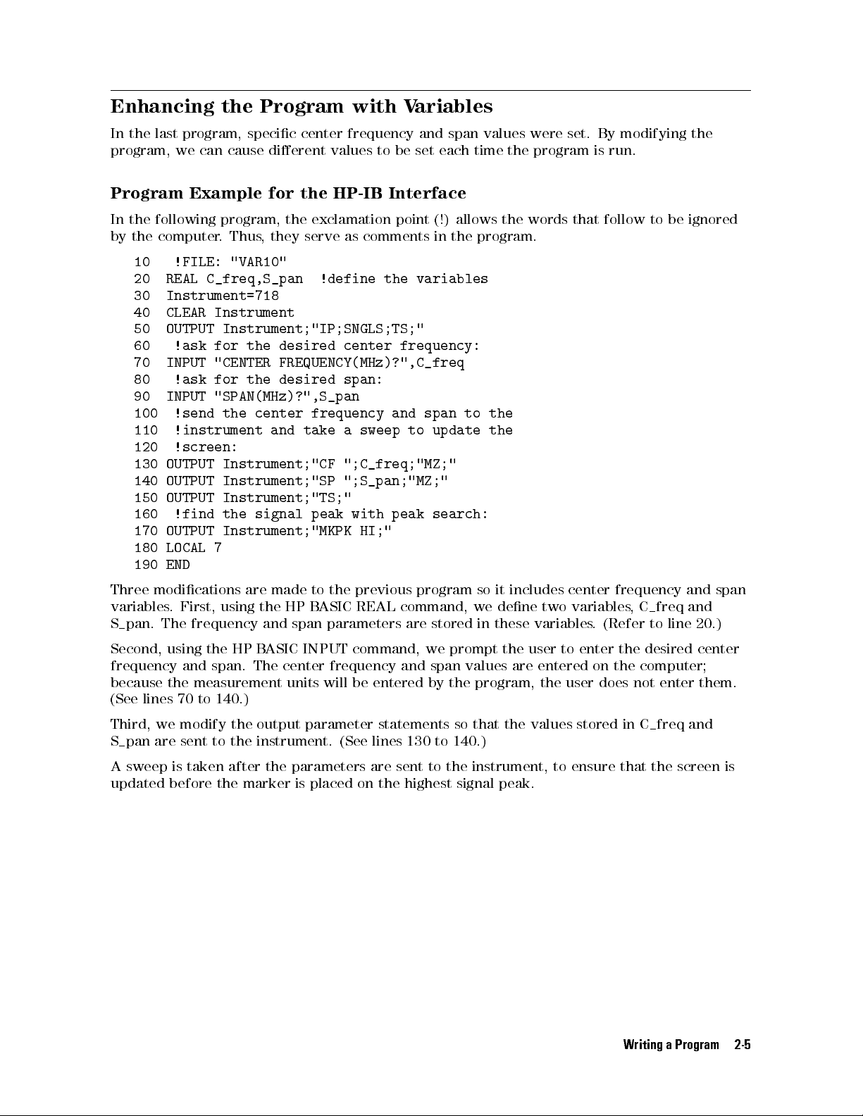
Enhancing

In

the

last

program,

we

the

program,

can

cause

Program

specic

center

dierent

with

frequency

values

V

ariables

and

span values were set. By modifying the

to

be

set each time the program is run.

Program Example for the HP-IB Interface

In the following program, the exclamation point (!) allows the words that follow to be ignored

by the computer. Thus, they serve as comments in the program.

10 !FILE: "VAR10"

20 REAL C_freq,S_pan !define the variables

30 Instrument=718

40 CLEAR Instrument

50 OUTPUT Instrument;"IP;SNGLS;TS;"

60 !ask for the desired center frequency:

70 INPUT "CENTER FREQUENCY(MHz)?",C_freq

80 !ask for the desired span:

90 INPUT "SPAN(MHz)?",S_pan

100 !send the center frequency and span to the

110

120

130

140

150

OUTPUT

OUTPUT

OUTPUT

!instrument

!screen:

Instrument;"CF

Instrument;"SP

Instrument;"TS;"

and

take

a

sweep

";C_freq;"MZ;"

";S_pan;"MZ;"

to

update

the

160 !find the signal peak with peak search:

170 OUTPUT Instrument;"MKPK HI;"

180 LOCAL 7

190 END

Three modications are made to the previous program so it includes center frequency and span

variables. First, using the HP BASIC REAL command, we dene two variables, C freq and

S pan. The frequency and span parameters are stored in these variables. (Refer to line 20.)

Second, using the HP BASIC INPUT command, we prompt the user to enter the desired center

frequency and span. The center frequency and span values are entered on the computer;

because the measurement units will be entered by the program, the user does not enter them.

(See

lines

70

to

140.)

Third,

we

modify

the

output

parameter

statements so that the values stored in C

freq

and

S pan are sent to the instrument. (See lines 130 to 140.)

A sweep is taken after the parameters are sent to the instrument, to ensure that the screen is

updated before the marker is placed on the highest signal peak.

Writing a Program 2-5

Getting

The

rst

section

F

or

example

Information

part

of

this

demonstrates

,

in

the

chapter

a

technique

second

from

demonstrated

for

getting

program

of this chapter, we placed a marker at the highest peak

the

Instrument

techniques

information

for setting instrument parameters. This

out

of the instrument.

of a trace and the value of the marker could be read in the upper right-hand corner of the

instrument

marker's

display

frequency

.

In

the following program, we will add some commands that will read the

and

amplitude

value and return those values to the computer.

Program Example for the HP-IB Interface

10 !FILE: "MKR"

20 REAL A_mpmarker,F_reqmarker !define variables

30 Instrument=718

40 OUTPUT Instrument;"IP;"

50 !set the output format of the instrument for

60 !real numbers:

70 OUTPUT Instrument;"TDF P;"

80 !set the instrument parameters:

90 OUTPUT Instrument;"SNGLS;"

100

110

120

130

140

OUTPUT

OUTPUT

OUTPUT

OUTPUT

!ask

Instrument;"CF

Instrument;"SP

Instrument;"TS;"

Instrument;"MKPK

the

instrument

300MZ;"

200MZ;"

HI;"

for

the

marker's

150 !amplitude value:

160 OUTPUT Instrument;"MKA?;"

170 !send the amplitude value to the computer:

180 ENTER Instrument;A_mpmarker

190 !ask the instrument for the marker's

200 !frequency value:

210 OUTPUT Instrument;"MKF?;"

220 !send the frequency value to the computer:

230 ENTER Instrument;F_reqmarker

240 !print the amplitude and frequency:

250 PRINT "THE SIGNAL PEAK IS ";A_mpmarker;

260

PRINT

"

dB



V

AT ";F_reqmarker/1.E+6;" MHz"

270 !set the instrument to continuous sweep mode:

280 OUTPUT Instrument;"CONTS;"

290 LOCAL 7

300 END

2-6 Writing a Program

First, using the HP BASIC REAL command, we dene two variables, A mpmarker and

F reqmarker. The amplitude and frequency values of the marker are stored in these variables.

(See line 20.)

Second, we set the output format of the instrument for real numbers with the instrument's

trace data format (TDF) command. (See line 70.) As in our original program, we set the center

frequency and span values. A sweep is taken and the marker is placed on the trace.

Next, we ask the instrument for the amplitude value of the marker.We have the instrument

send the marker amplitude value to the computer. Note that there can be only one instrument

query per programming line.We also ask the instrument for the frequency value of the marker,

and we have the instrument send the marker frequency value to the computer. (See lines 100

through

Finally, we print the values on the computer screen:

Before we end the program, we return the instrument to continuous-sweep mode and local

control.

230.)

"THE SIGNAL PEAK IS ... dBV AT ... MHz"

Writing a Program 2-7

Programming

Guidelines

1. Perform the measurement manually, keeping track of the sequence of functions used.

2. In the written program, execute an instrument preset (IP) and set single-sweep mode

(SNGLS) before setting other instrument functions.

3. Use variables for function values. List variables at the beginning of the program.

4. Activate instrument functions in logical order. Place quotation marks around instrument

commands

5.

After

or

activating

6.

The

query

7.

Use

apostrophe

exclamation

.

Separate

setting

instrument

markers

instrument

per

programming line.

can

commands

functions

.

return

only

with

semicolons

,

execute a take sweep (TS) command before reading data

.

one value per programming line. Do not have more than one

the exclamation point (!) to include comment lines when using HP BASIC. Use the

(')

or REM to create comment lines when using GW BASIC. (The use of the

point

and the apostrophe to create comment lines are dependent on the

controller and the programming language [not interface-dependent] and may be dierent for

your

system.)

2-8 Writing a Program

Programming Topics

What You'll Learn in This Chapter

This chapter contains the following advanced programming techniques and topics.

An example of moving and saving trace data from the instrument into the computer.

An example of how instrument states are saved with the computer, then returned to the

instrument.

An example of reading trace data from a computer disk.

An example of saving and recalling instrument states.

An example of returning the instrument to its former state.

A summary of using dierent formats for trace data transfers.

Many of the programming suggestions discussed in Chapter 2 have been incorporated into the

programs in this chapter.

3

Note

A general knowledge of the BASIC programming language is recommended before reading

this chapter. (Refer to your software documentation manuals.) Chapter 4 denes instrument

commands alphabetically.

All programming examples for the HP-IB interface in this chapter are written

in HP BASIC 4.0.

Programming Topics 3-1

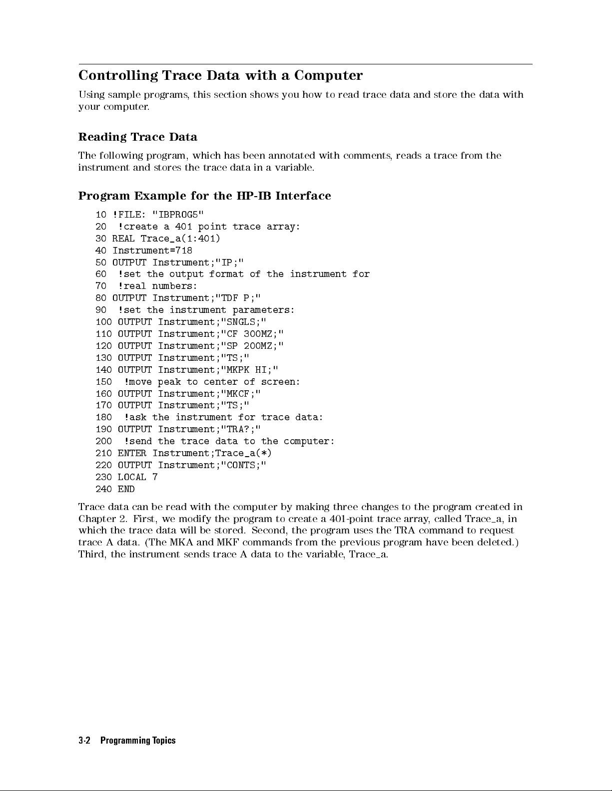
Controlling

Using

sample

your

computer

Trace

programs

.

,

this

Data

section

with

shows

a

Computer

you

how to read trace data and store the data with

Reading Trace Data

The following program, which has been annotated with comments, reads a trace from the

instrument and stores the trace data in a variable.

Program

10

20

30

40

50

Example

!FILE:

!create

REAL

"IBPROG5"

a

401 point trace array:

Trace_a(1:401)

Instrument=718

OUTPUT

Instrument;"IP;"

for

the HP-IB Interface

60 !set the output format of the instrument for

70 !real numbers:

80

OUTPUT

90

!set

100

OUTPUT

110

OUTPUT

120

OUTPUT Instrument;"SP 200MZ;"

130

OUTPUT Instrument;"TS;"

140

OUTPUT Instrument;"MKPK HI;"

Instrument;"TDF

the

instrument

parameters:

Instrument;"SNGLS;"

Instrument;"CF

P;"

300MZ;"

150 !move peak to center of screen:

160 OUTPUT Instrument;"MKCF;"

170 OUTPUT Instrument;"TS;"

180 !ask the instrument for trace data:

190 OUTPUT Instrument;"TRA?;"

200 !send the trace data to the computer:

210 ENTER Instrument;Trace_a(*)

220

230

OUTPUT

LOCAL

Instrument;"CONTS;"

7

240 END

Trace data can be read with the computer by making three changes to the program created in

Chapter 2. First, we modify the program to create a 401-point trace array, called Trace a, in

which the trace data will be stored. Second, the program uses the TRA command to request

trace A data. (The MKA and MKF commands from the

Third, the instrument sends trace A data to the variable

previous program have been deleted.)

, Trace

a.

3-2 Programming Topics

Saving

The

program

10

Trace

trace

data

modications

!FILE:

Data

in

the

previous

.

"IBPROG6"

program

can

be stored on a computer disk by making three

20 !create a 401 point trace array:

30

REAL

Trace_a(1:401)

40

Instrument=718

50

60

70

OUTPUT

!set

!real

Instrument;"IP;"

the

output

format of the instrument for

numbers:

80 OUTPUT Instrument;"TDF P;"

90 !set the instrument parameters:

100 OUTPUT Instrument;"SNGLS;"

110 OUTPUT Instrument;"CF 300MZ;"

120 OUTPUT Instrument;"SP 200MZ;"

130 OUTPUT Instrument;"TS;"

140

OUTPUT Instrument;"MKPK HI;"

150

!move peak to center of screen:

160

OUTPUT

170

OUTPUT

180

!ask the instrument for trace data:

Instrument;"MKCF;"

Instrument;"TS;"

190 OUTPUT Instrument;"TRA?;"

200 !send the trace data to the computer:

210 ENTER Instrument;Trace_a(*)

220 !create file to store trace

230 !file is 13 records long:

240

250

260

270

280

290

CREATE

!assign

ASSIGN

!send

OUTPUT

OUTPUT

BDAT

"DATA_A",13

path

for

the

file:

@File

trace

TO

"DATA_A"

data

to

the

@File;Trace_a(*)

Instrument;"CONTS;"

file:

300 LOCAL 7

310 !close file:

320 ASSIGN @File TO *

330 END

First, using the CREATE command, we create an empty le on the disk for storing the trace.

The le is 13 records long. (To determine the number of records, the 401-point trace is

multiplied by 8 bytes per point, the storage required for real numbers, then divided by 256

bytes per record. The result is rounded to the next largest integer.)

Next, we assign an input and an output path to the le DATA A. Then, we send the trace data

to the le. (See lines 260 through 280.) Finally, in line 320, we close the le.

Note

If a program containing the CREATE command is run twice, the computer will

report an error the second time because the le already exists.To prevent this

error, place an exclamation mark before the CREATE command to \comment

out" the line after the rst run. (See line 240.)

Programming Topics 3-3

Reading

If

we

want

process

and

stores

in

reverse

Trace

to

return

the

trace

.

Data

trace

The

in

data

following

an

array

from

to

a

Computer Disk

the instrument for later viewing, we must work the \saving"

program

variable

.

reads

a trace previously stored on a computer disk

Program Example for the HP-IB Interface

10 !FILE: "IBPROG7"

20 !create a 401-point trace array:

30 REAL Trace_a(1:401)

40 !assign path to the file with the

50 !trace in it:

60 ASSIGN @File TO "DATA_A"

70 !enter trace into variable Trace_a:

80 ENTER @File;Trace_a(*)

90 !close file:

100 ASSIGN @File TO *

110 END

First, in line 30, the program creates a 401-point trace array. Then, in line 60, the program

assigns

variable

a

path

Trace

to

a(*).

the

trace

le

.

Finally

, in line 80, the program sends the trace data to the

3-4 Programming Topics

Saving

The

later

stored

and

instrument's

to

streamline

in

one

of

Recalling

control

eight

test

state

settings

sequences

Instrument

(or

its

or

repeat

registers

in

States

\state")

can

manual

be saved with a computer and retrieved

measurements. Control settings can be

the instrument, in computer memory, or on a computer

disk.

The

rst

with

the

If

you

recall

its

trace

wish

state

program

current

data

(RCLS)

in

this section demonstrates techniques for saving an instrument state, along

trace

A data. The second program demonstrates how the state information and

is

read from the computer and returned to the instrument.

to save states in the instrument, see the descriptions of the save state (SAVES) and

commands in Chapter 4.

Saving the Instrument's State

The following two programs read and store a trace from the instrument.

Program Example for the HP-IB Interface

10

!FILE:

"IBPROG8"

20 !define 202 character string:

30 DIM Learn_string$[202]

40 !create 401-point array to store trace:

50 INTEGER Trace_a(1:401)

60 Instrument=718

70

!set

80

90

OUTPUT

!ask

output

Instrument;"TDF

instrument

format

for

for

trace

two

B;"

byte

data:

integers:

100 OUTPUT Instrument;"TRA?;"

110 !send trace to the computer:

120 ENTER Instrument USING "#,W";Trace_a(*)

130

!get

140

150

160

170

OUTPUT

ENTER

!create

CREATE

learnstring

Instrument;"OL;"

Instrument

file

BDAT

"STATE",4

to

from

USING

store

instrument:

"#,202A";Learn_string$

trace:

180 !assign path to the file:

190 ASSIGN @File TO "STATE"

200 !send trace to the file:

210 OUTPUT @File;Learn_string$,Trace_a(*)

220 !return output format to default mode:

230 OUTPUT Instrument;"TDF P;"

240 !close file:

250 ASSIGN @File TO *

260 END

The program stores the trace in the variable called Trace a(*). The state of the instrument is

stored in the variable Learn string$. These two variables are then saved in a le called STATE.

Finally, the le is stored on a disk.

Using the data stored in STATE, the instrument settings can be reset according to the saved

state. Then, using the stored trace data, trace data can be viewed on the display.

Line 30 gives the dimensions of the learn string using the HP BASIC DIM command. Learn

strings for the instrument require 202 bytes of storage space. Also see the output learn string

(OL) command.

Programming Topics 3-5

Line 70 uses TDF B to format the output in binary. Binary provides the fastest data transfer

and requires the least amount of memory to store data. Each data point is transferred in

binary as two 8-bit bytes. The data points are in the internal representation of measurement

data. (See \Dierent Formats for Trace Data Transfers" at the end of this chapter for more

information about trace data formats.)

When the trace and state data are sent from the instrument to the computer, they must be

formatted. Lines 120 and 150 format trace data with the HP BASIC USING command. In the

formatting statement, \#" indicates that the statement is terminated when the last ENTER

item is terminated. EOI (end-or-identify) and LF (line feed) are item terminators, and early

termination will result in an inaccurate learn string. \W" species word format. \202A"

indicates the size of the learn string.

Line 170 creates a le called STATE that is 4 records long. (To determine the number of records

for the computer in our example, the 401-point trace is multiplied by 2 bytes per point and the

202-byte learn string is added to give 1004 bytes total. This total is divided by 256 bytes per

record, resulting in 4 records.)

If

Note

the program containing the CREATE command is run twice, the computer

will report an error the second time because the le already exists.To prevent

this, place an exclamation mark before the CREATE command to \comment

out"

line

170

after

the

program

has been executed.

3-6 Programming Topics

Returning

The

following

the

Instrument

programs

read

a

trace

to

stored

its

Former State

in

a le and load it into a variable.

Program Example for the HP-IB Interface

10 !FILE: "IBPROG9"

20 !define 202 character string:

30 DIM Learn_string$[202]

40 !create 401 point array to store trace:

50 INTEGER Trace_a(1:401)

60 Instrument=718

70 !assign path to the file:

80 ASSIGN @File TO "STATE"

90 !get values for Learn_string$

100 !and Trace_a(*) from disk:

110 ENTER @File;Learn_string$,Trace_a(*)

120 !send learnstring to instrument:

130 OUTPUT Instrument;"IP DONE;"

140 ENTER Instrument

150 OUTPUT Instrument;Learn_string$

160

!set

170

180

190

200

OUTPUT

!prepare

!the

OUTPUT

single

Instrument;"SNGLS;"

computer:

Instrument;"TRA

sweep

instrument

mode:

for

a

#A";

trace

from

210 !send trace to the instrument

220 OUTPUT Instrument USING "#,W";802,Trace_a(*)

230 !view trace to see it was sent:

240 OUTPUT Instrument;"VIEW TRA;"

250 !close file:

260 ASSIGN @File TO *

270 END

The HP-IB program reads a trace stored in the le STATE, then loads it into the variable

Trace a(*).

First, the settings of the instrument that were stored in the variable LEARN$ are recalled. The

instrument

state

is

changed

to

the

same state as when the trace was stored. Then previously

stored trace data is returned to the instrument and the trace is viewed on the instrument

screen. Finally, line 220 uses the HP BASIC USING command to format the trace data.

Programming Topics 3-7

Dierent

Two

dierent

this

chapter

The

EMI

F

ways

(TDF

receiver

ormats

to

format

P

and

TDF

or

receiver

for

trace

B).

RF

Trace

data

This

section

Data Transfers

using

the TDF command were introduced earlier in

section describes all the available trace data formats.

provides

ve formats for trace data transfers: real

number (P) format, binary (B) format, A-block format, I-block format, and measurement units

(M)

format.

PFormat

The P format allows you to receive or send trace data in a real-number format. This is the

default format when the instrument is powered up. Numbers are in dBm, dBmV,dBV, volts,

or watts. The AUNITS command can be used to specify the amplitude units. Real-number data

may be an advantage if you wish to use the data later in a program. However, data transfers

using P format tend to be slow and take up a lot of memory (compared to binary format, the

P format can take up to four times the amount of memory). Data is transferred as ASCII type.

Although the instrument can send the trace data to the computer as real numbers, the trace

data cannot be sent back to the instrument without changing the trace data to measurement

units (integers). See the following example.

Example

This

Note

of

example

Using

sends

The

the

P

F

trace

data

instrument

ormat

to

the

must

computer

be

in

the

and back to the instrument using P format.

log

amplitude

1 REAL Trace_data(1:401)

10 OUTPUT 718;"IP;CF 300MHZ;SP 20MHZ;SNGLS;TS;"

20

OUTPUT

718;"TDF

P;TRA?;"

30 ENTER 718;Trace_data(*)

40 OUTPUT 718;"VIEW TRA;MOV TRA,0;"

50 OUTPUT 718;"RL?;"

60 DISP "PRESS CONTINUE WHEN READY"

70 PAUSE

80 ENTER 718;Ref_level

90 MAT Trace_data=Trace_data0(Ref_level)

100 MAT Trace_data=Trace_data*(100)

110 MAT Trace_data=Trace_data+(8000)

120 OUTPUT 718;"TRA ";

130 OUTPUT 718;Trace_data(*)

140 LOCAL 718

150 END

scale

to use the TDF P format.

Declare an array for trace data.

Take a measurement sweep.

A

ctivate

the P format, output

trace A data.

The computer receives trace A

data from the instrument.

To verify that the trace data is

transferred back to the instru-

ment, set trace A to zeros.

Determine the amplitude of the

reference level. The amplitude

of the reference level is used to

change the integers sent to the

instrument into real numbers

Get the reference level.

These lines change the real trace

data (stored in Trace data) into

integers (in measurement units).

Sends the trace data back to the

instrument in measurement units.

.

3-8 Programming Topics

The trace data is sent to the computer in parameter units. A parameter unit is a standard

scientic unit. For the TDF P format, the parameter unit depends on the current amplitude

units (dBm, dBmV,dBV,V, W). Use the AUNITS command to change the units.

For more detailed information about the P format, see the description for TDF in Chapter 4.

BFormat

The

B

format

provides

Each

data

representation

not

send

the

point

a

header

allows

fastest

you

data

is

transferred

of

measurement

to

receive

transfer

or

send

trace data in a binary format. The B format

and requires the least amount of memory to store data.

in binary as two 8-bit bytes. The data points are in the internal

units

(0 to 8000). Unlike the A-block format, the B format does

. An end-or-identify (EOI) is sent with the last byte of data.

Example of Using the B Format

This example sends trace data from the instrument in B format. The trace data format must be

changed to A-block format to return the trace data to the instrument. See following example.

Note

It is not possible to return data to the instrument using binary format. You

must

use

either A-block or I-block format to return the trace data to the

instrument.

10 INTEGER Tra_binary(1:401)

20 ASSIGN @Sa TO 718;FORMAT OFF

30

40

OUTPUT

OUTPUT

@Sa;"IP;CF

@Sa;"MDS

300MZ;SP

W;TDF

20MZ;SNGLS;TS;"

B;TRA?;"

50 ENTER @Sa;Tra_binary(*)

60 OUTPUT @Sa;"TDF A;"

70

OUTPUT

@Sa;"MOV

TRA,0;"

80 DISP "PRESS CONTINUE WHEN READY"

90 PAUSE

100 OUTPUT @Sa USING "#,K,W";"TRA#A",802

110

OUTPUT

@Sa;Tra_binary(*)

120 OUTPUT @Sa;"VIEW TRA;"

130 LOCAL 718

140 END

Tra binary stores the trace data.

Takes a measurement sweep.

Outputs

trace

A

data.

Changes the trace data format to A-

block format.

T

o

verify that the trace data is sent

back

to

the

zeros

into

instrument,

trace

A.

move

all

Prepares the instrument for the trace

data.

Transfers

the

trace

data back to the

instrument.

The result is transmitted as binary information. The MDS command can be used to change the

data format from two 8-bit bytes to one 8-bit byte

.For more detailed information about the

B format and the MDS command, see the descriptions for TDF and MDS in Chapter 4.

Binary data can be converted to dBm or volts.For example, use the following equation to

change the trace data (in measurement units) to a real logarithmic number (dBV):

dBV

=0(trace data08000)20:011+ reference level (in

dBV

)

To change the trace data (in measurement units) to linear data (volts):

volts =



reference level

8000



2

trace data

Programming Topics 3-9

The following programming converts binary data to dBV.

10 ! 8546 binary data to real numbers

20 Rcvr=718

30 ASSIGN @Rcvr_bin TO Sa;FORMAT OFF

40 INTEGER Trace_a(1:401)

50 OUTPUT Rcvr;"AUNITS DBUV;"

60 OUTPUT Rcvr;"RL?;"

70 ENTER Rcvr;Ref_lev

80 PRINT Ref_lev

90 OUTPUT Rcvr;"TDF B;TRA?;"

100 ENTER @Rcvr_bin;Trace_a(*)

110 ! now the instrument has all the data

120 ! to determine the measured trace data

130 REAL Trace_a_real(1:401)

140 MAT Trace_a_real= Trace_a-(8000) ! Results in below ref

150 ! level

160

MAT

Trace_a_real=

Trace_a_real*(.01)!

now

in hundredths of db

170 ! below ref lev

180 MAT Trace_a_real= Trace_a_real+(Ref_lev)

190 FOR I=1 TO 401

200 PRINT Trace_a_real(I)

210 NEXT I

220

The

END

following

programming

converts

binary

data

to

volts

.

10

20

30

40

50

60

70

!

8546

Rcvr=718

ASSIGN

INTEGER

OUTPUT

OUTPUT

ENTER

Rcvr;Ref_lev

binary

@Rcvr_bin

data

to

TO

Rcvr;FORMAT OFF

Trace_a(1:401)

Rcvr;"LN;AUNITS

Rcvr;"RL?;"

real

V;"

numbers

(linear)

80 Ref_lev_factor=Ref_lev/8000

90 OUTPUT Rcvr;"TDF B;TRA?;"

100 ENTER @Rcvr_bin;Trace_a(*)

110 ! now the instrument has all the data

120 ! to determine the measured trace data

130 REAL Trace_a_real(1:401)

140 MAT Trace_a_real= Trace_a*(Ref_lev_factor)

150 FOR I=1 TO 401

160 PRINT Trace_a_real(I)

170 NEXT I

180 END

A-Block Format

The A-block format is similar to binary format in that each data point is sent as two 8-bit bytes

(this, too, is in the internal representation of measurement data). A-block format also transfers

a four-byte header before the 401 points of trace data. These bytes are the ASCII character

\#", \A", and two-byte number representing the length of the trace data, followed by the data

bytes.

3-10 Programming Topics

Example of Using the A-Block Format

This example sends trace data from the instrument to the computer and back to the instrument

in A-block format.

10 INTEGER Tra_binary(1:401)

20

DIM

Header$[4]

30 OUTPUT 718;"IP;CF 300MZ;SP 20MZ;SNGLS;TS;"

40 OUTPUT 718;"MDS W;TDF A;TRA?;"

50 ENTER 718 USING "#,4A,401(W)";Header$,Tra_binary(*)

60

PRINT

"PRESS

CONTINUE

TO

RETURN DATA TO THE INSTRUMENT"

70 PAUSE

80

OUTPUT 718;"IP;TS;VIEW TRA;"

90

OUTPUT

718;"TDF

A;"

100 OUTPUT 718 USING

"#,K,W,401(W)";"TRA#A",802,Tra_binary(*),";"

110

END

The

transferred

byte

(MSB)

the

terminal

your

computer

trace

length

you

and

are

documentation

data

the

using,

consists

least

signicant

the

data

to

of

#A

,

bytes

determine

a

two-byte

byte

may

the

(LSB)

appear

number

length,

as

representing

and

symbols

numeric value of the data bytes.

the

data

instead

Declare an array for trace

data.

Declare

#,

LSB

A,

length

a

string for the

MSB

length,

header

and

.

Take a measurement sweep.

Send trace A to the com-

puter in A-block format.

The computer receives

the header and the trace

data.

View trace A.

The instrument receives

the trace data from the

computer

the

bytes

of

.

most

signicant

.

Depending on

numbers. Consult

F

or

more

detailed

descriptions

I-Block

The

F

I-block

ormat

for

TDF

format

information

and

MDS

transfers

about

the A-block format and the MDS command, see the

in

Chapter 4.

data points as two 8-bit bytes in the internal representation of

measurement data. In addition to transferring trace data, I-block format also transfers the

characters \#" and \I". These characters indicate that the trace data is in I-block format. The

I-block format allows the instrument to accept up to 401 points of trace data when using

I-block format. Fewer than 401 points of trace data can be specied, and the instrument

will accept data until an EOI signal is sent to it. Therefore, returning the trace data to the

instrument requires an important instruction, END

Example of Using the I-Block F

ormat

. (See following example

.)

This example sends trace data from the instrument to the computer and back to the instrument

in I-block format.

10 INTEGER Tra_binary(1:401)

Declare an array for trace

data.

20 DIM Header$[2]

Declare an array for #,

I header.

30 OUTPUT 718;"IP;CF 300MZ;SP 20MZ;SNGLS;TS;"

40 OUTPUT 718;"TDF I;TRA?;"

Take a measurement sweep.

Send trace A data in I-

block format.

Programming Topics 3-11

50 ENTER 718 USING "#,2A,401(W)";Header$,Tra_binary(*)

The computer receives

the header and trace A

data.

60 PRINT "PRESS CONTINUE TO RETURN DATA TO THE INSTRUMENT"

70 PAUSE

80 OUTPUT 718;"IP;TS;VIEW TRA;"

90

OUTPUT

718;"TDF

I;"

100 OUTPUT 718 USING "#,K,W,401(W)";"TRA#I",

Tra_binary(*)END

110

END

View trace A.

The trace data is returned

to

the

instrument.

The END statement in line 100 sends the instrument the last data byte stored in the array and

sets the HP-IB EOI line \true," as required by the I-block format.

The transferred trace data consists of#I, followed by data bytes until the EOI line is set true.

For more detailed information about the I-block format and the MDS command, see the

descriptions for TDF and MDS in Chapter 4.

M

Format

The M format is for sending trace data only. It formats the trace data in the internal format

used by the instrument, also known as measurement units. Refer to Figure 3-1 .

The displayed amplitude of each element falls on one of 8000 vertical points with 8000 equal to

the reference level. For log scale data, each point is equal to 0.01 dB. The peak of the signal in

Figure

divisions

6000).

The

reached

3-1

In

range

is

equal

below

linear

of

internal

during

to

the

mode

trace

72

dB



reference

,

each

data

is

math

operations

V

for

level.

point

0

32,768

the

EMI receiver (87 dBV for the RF lter section) or two

In

measurement

has

a

resolution

to

only

+32,767.

.

units

,

it

is

equal to 6000 (800002000 =

of [reference level in volts divided by 8000].

In practice however, the range limits can be

3-12 Programming Topics

Figure

3-1.

Measurement Unit Range and Trace Amplitudes

Table 3-1. Measurement Units

Index

Number

1 A

2 The area from 8000 (reference level) to 8160 (1.6 dB above reference level)

3 The area from 0 to 8000 represents the displayed range for trace amplitude

4 A number within the range of 0 to032,768 measurement units is clipped at

number within the range of 8161 to 32,767 measurement units is clipped at

upper limit.

represents the amount a trace element's amplitude can exceed the top graticule

and still be displayed without clipping.

data. The range of 0 to 8000 varies according to the amplitude scale of the

instrument as follows:

In 10 dB/division, the range is from 0 to 8000.

In 5 dB/div, the range is from 4000 to 8000.

In 2 dB/div, the range is from 6000 to 8000.

In 1 dB/div, the range is from 7000 to 8000.

lower limit.

Description

Programming Topics 3-13

Example of Using the M Format

This example sends trace data from the instrument to the computer in M format.

10 INTEGER A(1:401)

30 OUTPUT 718;"IP;CF 300MZ;SP 20MZ;SNGLS;TS;"

40 OUTPUT 718;"TDF M;TRA?;"

50 ENTER 718;A(*)

60

PRINT

A(*)

Dimension array A.

Take a measurement sweep.

Send trace A data in M format.

The computer receives the trace data.

Print trace data.

70 END

Note

functions

are

done

using

measurement

units

.SeeTable 4-4 for a

All

trace

math

list of all trace math functions.

The result is in measurement units (032768 to +32767).

Table 3-2 summarizes the dierent trace data formats.

Table 3-2. Summary of the Trace Data Formats

Trace

Description Remarks

Data

F

ormat

TDF

Real

P

F

ormat

Number

Instrument

data

back

to

measurement

must

the

units

be

in

log

scale

instrument,

.

the

to

data

use

TDF

must

P

.To send the trace

be

converted

to

TDF B Binary Format Fastest format for trace data transfers. Use the A-block format to

send data back to the instrument.

TDF A A-Block Data

Format

TDFII-Block

F

ormat

Data

TDF M Measurement

Data Format

Trace data preceded by \#," \A," and a two-byte number.To use

the A-block format for sending data, you must provide the

number of data bytes.

Trace

data

preceded

by

\#,"

and

\I."

TDF M cannot be used to send trace data back to the instrument.

3-14 Programming Topics

Programming Commands

What You'll Learn in This Chapter

This chapter is a reference for the EMI receiver and receiver RF section that lists all

parameters for each of the programming commands available.

To nd a programming command that performs a particular function, rst refer to Table 4-4

where commands are categorized by function. Once the desired command is found in the

functional index, refer to the description for the command in this chapter.

This chapter includes the reference tables listed below:

Table 4-1, Syntax Elements

Table 4-2, Characters and Secondary Keywords (reserved words)

Table 4-3, Summary of Compatible Commands

T

able

4-4

,

Functional

Index

4

Programming Commands 4-1

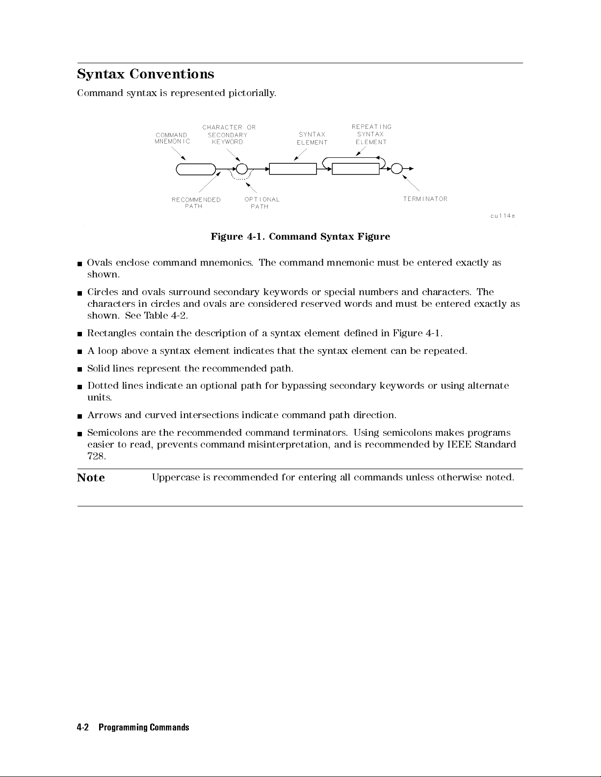
Syntax

Conventions

Command

syntax

is

represented

pictorially

.

Figure 4-1. Command Syntax Figure

Ovals enclose command mnemonics. The command mnemonic must be entered exactly as

shown.

Circles and ovals surround secondary keywords or special numbers and characters.The

characters in circles and ovals are considered reserved words and must be entered exactly as

shown. See Table 4-2.

Rectangles

A

loop

Solid

above

lines

contain

a

syntax

represent

the

description

element

the

recommended

of

a

indicates

syntax

that

path.

element

the

syntax

dened

in

Figure 4-1.

element can be repeated.

Dotted

units

Arrows

lines indicate an optional path for bypassing secondary keywords or using alternate

.

and curved intersections indicate command path direction.

Semicolons are the recommended command terminators. Using semicolons makes programs

easier to read, prevents command misinterpretation, and is recommended by IEEE Standard

728.

Note

Uppercase is recommended for entering all commands unless otherwise noted.

4-2 Programming Commands

Syntax Elements are shown in the syntax diagrams as elements within rectangles.

Table 4-1. Syntax Elements

Syntax Component Denition/Range

instrument command Any instrument command in this chapter, with required parameters and terminators.

character SP!

"

#

$

%

&

'

(

)

+,/0123456789: ;ABCDEFGHIJKLMNOPQRST

UVWXYZ[n]? ` a b c d e f g h i j k l m n o p q r s t u v w x y z (Characters are a

subset of data byte.)

character & EOI 8-bit byte containing only character data and followed by end-or-identify (EOI)

condition, where the EOI control line on HP-IB is asserted to indicate the end of the

transmission.

END

signies

the

EOI

condition.

data byte 8-bit byte containing numeric or character data.

data byte & EOI 8-bit byte containing numeric or character data followed by end-or-identify (EOI)

condition, where the EOI control line on HP-IB is asserted to indicate the end of the

transmission.

END

signies

the

EOI

condition.

delimiter ~jn@=/^$%;!':"&

Matching characters that mark the beginning and end of a character string, or a list of

user-dened functions or instrument commands. Choose delimiting characters that are

not

used

within

the

string

they

delimit.

digit 0

1

23456789

lsb length Represents the least signicant byte of a two-byte word that describes the number of

bytes

returned

or

transmitted.

See

msb length.

msb length Represents the most signicant byte of a two-byte word that describes the number of

bytes

returned or transmitted. See lsb length.

number Expressed as integer, decimal, or in exponential (E) form. Real Number Range:

1.797693134862315

Up

to

15

signicant

Numbers may be as small as62.225073858507202210

2

308

10

gures

,

including

allowed.

0.

0

308

Integer Number Range:032,768 through +32,767

6

output termination Carriage return (CR) and line feed (LF), with end-or-identify (EOI) condition. ASCII

codes 13 (carriage return) and 10 (line feed) is sent via HP-IB, then the end-or-identify

control

line

on HP-IB sets to indicate the end of the transmission.

predened function BITF, CNTLI, CORREK, DONE, HN, LIMIFAIL, MEAN, MEANTH, MINPOS, MKBW,

PEAKS,

PKPOS,

PWRBW

,

REV

, RMS, SER, STB, SUM, SUMSQR, TRCMEM, VARIANCE.

A predened function is an instrument command that returns a number that can be

operated on by other instrument commands. Insert a predened function into a

command statement where predened function appears

If a predened function takes a parameter (for example

in the command syntax chart.

, PKPOS TRA), it can be used

only as the last parameter of a instrument command that has two or more predened

functions as parameters

.F

or example, MPY V

AR,PKPOS TRB

,HAVE DISK; is illegal,

but MPY V AR,DONE,HAVE DISK; is not.

Programming Commands 4-3

Table 4-1. Syntax Elements (continued)

Syntax

Component

Denition/Range

predened variable The values of the following variables change depending on the current instrument

settings

. Each variable represents the value of the command function that has the

same name as the variable.

AMB, AMBPL, ANNOT,AT,AVBW,BAUDRATE, CF, CNTLA, CNTLB, CNTLC, CNTLD,

COUPLE,

DATEMODE, DET,FA, FB, FMGAIN, FOFFSET, GR, GRAT, IFBW, INZ, LG,

LIMIDISP, LIMIMODE, LIMIREL, LIMITEST, MEASURE, MF, MKA, MKACT, MKF,

MKFCR,

MKN,

MKNOISE,

MKP

,

MKP

A

USE,

MKPX, ML, MKTRACK, MSI, NRL,

POWERON, PREAMPG, PRNTADRS, PSTATE, RB, RL, RLPOS, ROFFSET, SETDATE,

SETTIME, SP, SQLCH, SRCALC, SRCAT, SRCNORM, SRCPOFS, SRCPSTP, SRCPSWP,

SRCPWR,

SRCTK,

SS,

ST, SWPCPL, TH, TIMEDATE, TIMEDSP,VB, VBR, WINZOOM,

ZMKCNTR, ZMKSPAN.

trace

element

V

alue

contained

in

one

trace point. Notated as TRA[N] where N species the point

position in the trace array.Values for N are 1 to 401 (for traces A, B, C) or 1 to 2047

(for traces specied by TRDEF). The same values apply to trace B (TRB[N]), trace C

(TRC[N]),

and user-dened traces (LABEL[N]).

trace range Values contained in trace segment. Multi-point segments are notated as TRA[N,M],

where N and M are end points of a segment and specify point positions in trace array.

Values for N or M are 1 to 401 (for traces A, B, C), or 1 to the length of a trace as

specied

and

by

TRDEF

user-dened

.

The

traces

same

values

(LABEL[N,M]).

apply to trace B (TRB[N,M]), trace C (TRC[N,M]),

Single-point

segments

are

notated

the

same

the trace element above.

units Represent

standard

scientic

units

.

Frequency Units: GHZ or GZ, MHZ or MZ, KHZ or KZ, HZ

Amplitude

Units:

DB, DM, DBMV,DBPT,DBUA, DBUV, DBUAM, DBUVM, G, PT,

V

,

MV

,

UAM, UV,UVM,W,MW,UW

Time Units: SC, MS, US

Current Units: A, MA, UA

Impedance Units: OHM

as

user-dened trace A label 2 to 11 characters long that is dened by the TRDEF command. Choice of

characters is A through Z and the underscore( ). The underscore should be used as the

second character of the label. Omitting the underscore, or using the underscore as

other than the second character in a label, is not recommended.

user-dened

variable

A

label

2

to

11

characters long that is dened by the VARDEF command. Choice of

characters is A through Z and the underscore( ). The underscore should used as be the

second character of the label. Omitting the underscore, or using the underscore as

other than the second character in a label, is not recommended.

4-4 Programming Commands

In the syntax diagrams, characters and secondary keywords are shown within circles or ovals.

Characters and secondary keywords must be entered exactly as shown.

Table 4-2. Characters and Secondary Keywords (Reserved Words)

Element Description

A Amp (unit) or A-block data eld

ABSHZ Absolute

Hz

(unit)

AC Alternating current

ALL All

AM Amplitude

modulation

AMP Amplitude

AMPCOR Amplitude

correction

AUTO Auto couple or set to automatic

AVG Average

B 8-bit byte or binary format

BOTH Both odd and even frames trigger

BW Black

and

white

c Cable amplitude correction factors

CNT Counter-lock

COLOR Color

CPL Couple

d Downloadable

DB Decibel

DBM Absolute

DBMV Decibel

DBUV Decibel

DC Direct

DEL

T

A

Delta

programs

(unit)

decibel milliwatt (unit)

millivolt

microvolt

(unit)

(unit)

current

DISP Display

DM Absolute

DMY Day

,

month,

decibel

year

milliwatt

format

(unit)

DN Decreases parameter one step size

DUMP Dump

e Setup

EDGE Triggers

le

on

the

edge

of the trigger input

EP Pauses program for data entry from instrument front panel

EQ Equal to

EVEN Even video frame

EXT External trigger

FADC Fast analog-to-digital converter (ADC)

FETCH Fetch

FFT Fast Fourier transform

FIXED Fixed

FLAT Flat

FLATTOP Flat top lter window

FMD Frequency modulation demodulator

Programming Commands 4-5

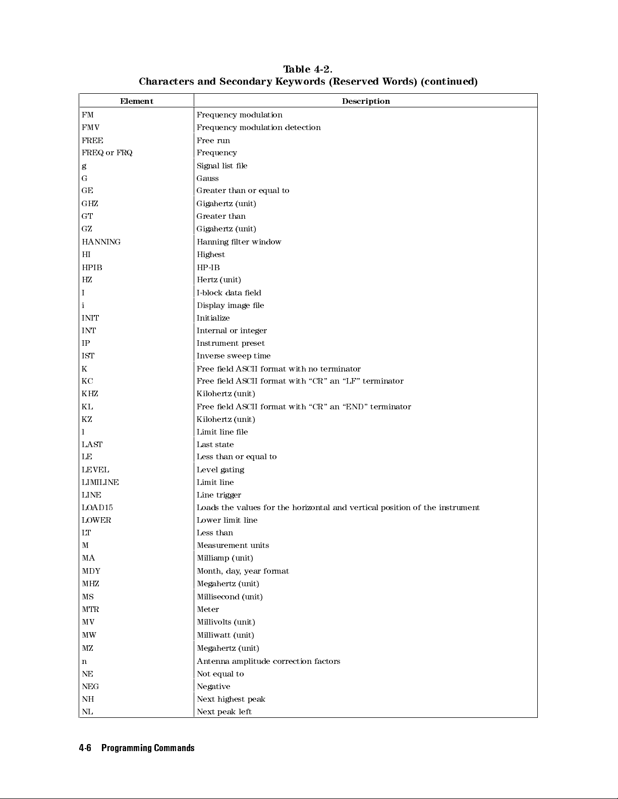
Table 4-2.

Characters and Secondary Keywords (Reserved Words) (continued)

Element Description

FM Frequency modulation

FMV Frequency modulation detection

FREE Free run

FREQ or FRQ Frequency

g Signal

list

le

G Gauss

GE Greater than or equal to

GHZ Gigahertz

(unit)

GT Greater than

GZ Gigahertz (unit)

HANNING Hanning lter window

HI Highest

HPIB HP-IB

HZ Hertz (unit)

I I-block data eld

i Display

image

le

INIT Initialize

INT Internal or integer

IP Instrument preset

IST Inverse

K Free

KC Free

KHZ Kilohertz

KL Free

eld

eld

eld

sweep

ASCII

ASCII

(unit)

ASCII

time

format

format

format

with

no

terminator

with

\CR"

an

\LF"

terminator

with

\CR" an \END" terminator

KZ Kilohertz (unit)

l Limit line le

LAST Last

state

LE Less than or equal to

LEVEL Level gating

LIMILINE Limit line

LINE Line trigger

LOAD15 Loads the values for the horizontal and vertical position of the instrument

LOWER Lower limit line

LT Less than

M Measurement units

MA Milliamp (unit)

MDY Month, day

, year format

MHZ Megahertz (unit)

MS Millisecond (unit)

MTR Meter

MV Millivolts (unit)

MW Milliwatt (unit)

MZ Megahertz (unit)

n Antenna amplitude correction factors

NE Not equal to

NEG Negative

NH Next highest peak

NL Next peak left

4-6 Programming Commands

Table 4-2.

Characters and Secondary Keywords (Reserved Words) (continued)

Element Description

NONE No units

NR Next peak right

NRM

or

NORMAL

Normal

o Other amplitude correction factors

OA Output amplitude

ODD Odd

video

frame

trigger

OFF Turns o function

ON Turns on function

P P

arameter

units

PER Period

PKAVG Peak average

PKPIT P

eak

pit

POINT Point

POS Positive

PSN Position

PT pico Tesla

RECALL Recall operation

RS232 RS-232

s State

SA Signal

SA

VE

SC Seconds

Save

interface

le

analysis

operation

(unit)

SLOPE Slope

SMP Sample

detection

mode

SP Space

SR Stimulus response

STATE State register

STEP Step key ability

STORE Store

SWT Sweep time

t Trace le

TG Tracking generator

TRA Trace A

TRB Trace B

TRC Trace C

UA Microamp (unit)

UAM Microamps per meter

UNCPL Uncouple

UNIFORM Uniform lter window

UP Increases the parameter one step size

UPLOW Upper and lower limit lines

UPPER Upper limit line

US Microseconds (unit)

UV Microvolts (unit)

UVM Microvolts per meter

UW Microwatt (unit)

Programming Commands 4-7

Table 4-2.

Characters and Secondary Keywords (Reserved Words) (continued)

Element Description

V Volts (unit)

VERTICAL V

VID Video trigger

W W

YTF YIG-tuned lter

XTAL Crystal

* Asterisk

; Semicolon (ASCII code 59)

, Comma (ASCII code 44)

0 O

1 On (command argument)

50 50

75 75

? Returns a query response containing the value or state of the associated parameter.The

ertical

triggering

atts

or word (for MDS command)

(used

as

a

wildcard)

(command

query response is followed by a carriage-return/line-feed.

argument)

4-8 Programming Commands

The alternate commands (listed in the left column of Table 4-3) provide compatibility with

commands used by the HP 8566A/B, HP 8568A/B, and HP 70000 Series instruments.The

equivalent commands for the HP 8542E/HP 8546A EMI receiver or HP 85422E/HP 85462A

receiver RF section are listed in the right column.

Table 4-3. Summary of Compatible Commands

Alternate

Description HP

8546A/HP

Commands

A1 Clear write trace A CLRW TRA

A2 Max hold trace A MXMH TRA

A3 Store and view trace A VIEW TRA

A4 Store

and

blank

trace

A

BLANK

B1 Clear write trace B CLRW TRB

B2 Max

hold

trace

B

MXMH

B3 Store and view trace B VIEW TRB

B4 Store and blank trace B BLANK TRB

C1 Trace A minus trace B o AMB OFF

C2 Trace A minus trace B on AMB ON

CA Coupled input attenuation ATAUTO

CR Coupled resolution bandwidth IFBW AUTO

CS Coupled step size SS AUTO

CT Coupled

CV Coupled

sweep

video

time

bandwidth

ST

A

A

VBW

UTO

E1 Peak search MKPK HI

E2 Enter marker into center frequency MKCF

E3 Enter

E4 Enter

marker

marker

EX Exchange

delta

amplitude

trace

into

center

frequency

into

reference

A

and

B

step size

level

MKSS

MKRL

AXB

KSA dBm amplitude units AUNITS DBM

KSB dBmV amplitude units AUNITS DBMV

KSC dB

KSD V



V

olt

amplitude

KSE Screen

amplitude

title

units

units

A

UNITS

A

UNITS

TITLE

KSG Video average on VAVG ON

KSH Video average o VAVG OFF

KSM Marker noise MKNOISE

KSO Marker value to span MKSP

KSZ Reference level oset ROFFSET

KSc Trace A plus trace B into trace A APB

KSi Exchange trace B and C BXC

KSl Trace B into trace C BTC

KSm Graticule o GRAT OFF

KSn Graticule on GRATON

KSo Annotation o ANNOT OFF

KSp Annotation on ANNOT ON

L0 Display line o DL OFF

Command

TRA

TRB

A

UTO

DBUV

V

8542E

Programming Commands 4-9

Table 4-3. Summary of Compatible Commands (continued)

Alternate

Commands

M1 Marker

o

Description HP 8546A/HP 8542E

Command

MKOFF

M2 Marker normal MKN

M3 Marker delta MKD

MA Marker amplitude MKA?

MC Marker

count

MKFC

MT0 Marker track o MKTRACK OFF

MT1 Marker track on MKTRACK ON

O1 Output format, in real number format TDF P

O2 Output format, in binary format, two bytes (word) per

TDF B;MDS W

element

O3 Output format, in measurement data format TDF M

TDF

O4 Output

format,

in

binary

format,

1

byte per element

B;MDS

R1 Activates illegal command service request only RQS 32

R2 Activates end-of-sweep, illegal command RQS 36

R3 A

R4 A

RC Recall

S1 Sweep

S2 Sweep

SV Save

ctivates broken hardware, illegal command

ctivates

state

continuous

single

state

T0 Threshold

T1 Trigger

T2 Trigger

units-key pressed, illegal command

o

mode

free

run

mode line

RQS

RQS

RCLS

CONTS

SNGLS

SA

VES

TH

OFF

TM

FREE

TM

LINE

40

34

T3 Trigger mode external TM EXT

T4 Trigger mode video TM VID

B

4-10 Programming Commands

This functional index categorizes the programming commands by the type of function that the

command performs. The functional index contains the following information: the programming

command mnemonic, the softkey or front-panel key that corresponds to the command's

function, and a brief denition of the command. Once the desired command is found, refer

to the alphabetical listing of commands later in this chapter for more information about the

command.

Table 4-4. Functional Index

Function

Category

AMPLITUDE

AUTO COUPLING

Command Corresponding

Description

Key Function

ARNG

AT

AUNITS

COUPLE

INZ

LG

LN

ML

4

AUTO RANGE

FFFFFFFFFFFFFFFFFFFFFFFFFFFFFFFFFFFF

ATTEN AUTO MAN

FFFFFFFFFFFFFFFFFFFFFFFFFFFFF

Amptd Units

F

F

F

F

FFFFFFFFFFFFFFFFFFFFFFFFFFF

COUPLE

FFFFFFFFFFFFFFFFFFFFFFFFFFFFFFFFFFFFFFF

INPUT Z 50 75

FFFFFFFFFFFFFFFFFFFFFFFFFFFFFFFFFF

SCALE

LOG

is

F

F

F

F

F

F

F

F

F

F

F

F

F

FFFFFFFFFFFFFFFFFFFFF

SCALE

is

underlined)

F

F

F

F

F

F

F

F

FFFFFFFFFFFFFFFFFFFFF

MAX

MXR

5

AC

DC

LOG

LIN

underlined)

LOG

LIN

LVL

(when

(when

Turns the autorange function on or o.

Species RF input attenuation.

Species amplitude units for input,

output, and display.

Selects

direct-current

(dc)

coupling or

alternating-current (ac) coupling.

Species the value of input impedance

expected at the active input port.

Species

as

the

logarithmic

vertical graticule divisions

units

,

without

the reference level.

LIN

Species

as

linear

the

units

vertical

,

without

graticule

changing

reference level.

Species

the

maximum

signal

changing

divisions

the

level

that

is applied to the input mixer for a signal

that is equal to or below the reference

level.

NRL Sets

O

VLD

PREAMP

PREAMPG

F

F

F

F

F

F

F

FFFFFFFFFFFFFFFFFFFFFF

OVLD

ON

F

F

F

F

F

F

F

F

F

F

FFFFFFFFFFFFFFFFFFFFFFFF

PREAMP

F

F

F

F

F

F

F

F

F

F

F

FFFFFFFFFFFFFFFFFFFFFFFFFFFFFF

EXTERNAL

OFF

ON

OFF

PREAMPG

the

Enables

Switches

out

of

the

Subtracts

normalized

or

disables

the

system

input

path.

a

positive

reference

overload

preamplier

or

negative

level.

detection.

in

and

preamplier gain value from the

displayed signal.

Performs a preselector peak.

PP

F

1

FFFFFFFFFFFFFFFFFFFFFFFFFFFF

PRESEL PEAK

RANGE Puts highest signal on display close to

the

reference

level.

RESETRL Resets the reference level to its

instrument preset level.

Species the amplitude value of the

reference level.

Osets all amplitude readouts without

RL

ROFFSET

FFFFFFFFFFFFFFFFFFF

REF LVL

FFFFFFFFFFFFFFFFFFFFFFFFFFFFFFFFFFFF

REF LVL OFFSET

aecting the trace.

UNRANGE Restores reference level to the value set

prior to RANGE command.

for the AMPCOR correction factors.

Couples the active functions

XUNITS

AUTO

FFFFFFFFFFFFFFFFFFFFFFFFFFFFFFF

Edit Antenna

FFFFFFFFFFFFFFFFFFFFF

AUTO ALL

functions Selects the transducer conversion units

automatically.

1

For an HP 8546A/HP 85462A only.

Programming Commands 4-11

Table 4-4. Functional Index (continued)

Function

Category

A

UXILIARY

CONTROL

Command Corresponding

Key Function

F

F

F

F

F

F

BYP

ASS

CALSW

CNTLA

CNTLB

CNTLC

CNTLD

CNTLI

DEMOD

FMGAIN

1

2

2

2

2

FFFFFFFFFFFFFFFFFFFFFFFFFFFFFF

INPUT

2

F

FFFFFFFFFFFFFFFFFFFFFFFFFFFFFFFFFFFFFF

VIEW CAL ON OFF

F

FFFFFFFFFFFFFFFFFFFFFFFFF

CNTL A 0 1

F

FFFFFFFFFFFFFFFFFFFFFFFFF

CNTL B 0 1

FFFFFFFFFFFFFFFFFFFFFFFFFF

CNTL C 0 1

FFFFFFFFFFFFFFFFFFFFFFFFFF

CNTL D 0 1

F

FFFFFFFFFFFFFFFFFFFFFFFFFFFFFFFFFFF

DISPLAY CNTL I

FFFFFFFFFFFFFFFFFFFFFFFFFFFFF

DEMODON OFF

FFFFFFFFFFFFFFFFFFFFFFFFFFFFF

DEMOD AM FM

F

F

F

F

F

F

F

F

F

F

F

F

FFFFFFF

FM

GAIN

BYPASS

,

Switches

path.

Switches the 300 MHz calibrator signal.

Sets the control line A of the auxiliary

interface

Sets the control line B of the auxiliary

interface

Sets the interface control line C of the

auxiliary

Sets the interface control line D of the

auxiliary

Returns a \1" when the interface

control

high,

and \0" if the line is low.

Turns the demodulator on or o, and

selects between AM, FM, or quasi-peak

demodulation.

Sets

the

Description

in

and

high or low.

high

or low.

interface

interface

line

I

of

total

FM

out

of

the bypass input

high

high

the

auxiliary

frequency

or

low

or

low

.

.

interface

deviation

for full screen demodulation.

MEASURE Determines

signal

analysis

the

,

type

of measurement:

stimulus

response

,

or

signal normalization.

NRL Sets the normalized reference level.

1

RFIN

1

RFINLK

RLPOS Selects

SPEAKER

SQLCH

SRCALC

SRCAT

4

5

INPUT

F

F

F

FFFFFFFFFFFFFFFFFFFFFFFFFFFFFFFFFFFF

INPT LCK ON OFF

FFFFFFFFFFFFFFFFFFFFFFFFFFFFFFFFFFFF

SPEAKER ON OFF

FFFFFFFFFFFFFFFFFFF

SQUELCH

F

F

F

F

F

F

F

F

F

F

F

FFFFFFFFFFFFFFFFFF

ALC

INT

EXT

F

FFFFFFFFFFFFFFFFFFFFFFFFFFFFFFFFFFFFFFFF

SRC ATN MAN AUTO

Species

lter

signal

section.

path

through

the

RF

Enables or disables tuning limits based

on

RF

lter

section input.

the

position of reference level.

Turns on or o the internal speaker.

Sets the squelch level.

Selects

internal

or

external

leveling

for

the tracking generator.

Attenuates the source output level.

SRCNORM Subtracts trace B from trace A, adds the

display line, and sends the result to

trace

A.

Osets the source power level readout.

Selects the source-power step size

.

Selects sweep range of the source

output.

Selects the source power level.

Adjusts tracking of source output with

instrument sweep

.

Adjusts tracking of source output with

instrument sweep.

Selects a stimulus-response (SR) or

SRCPOFS

SRCPSTP

SRCPSWP

SRCPWR

SRCTK

SRCTKPK

SWPCPL

FFFFFFFFFFFFFFFFFFFFFFFFFFFFFFFFFFFF

SRC PWR OFFSET

FFFFFFFFFFFFFFFFFFFFFFFFFFFFFFFFFFFFFFFFF

SRC PWR STP SIZE

F

FFFFFFFFFFFFFFFFFFFFFFFFFFFFFFFFFFF

PWR SWP ON OFF

F

FFFFFFFFFFFFFFFFFFFFFFFFFFFFFFFFFFF

SRC PWR ON OFF

F

FFFFFFFFFFFFFFFFFFFFFFFFFFFFFFFFFFF

MAN TRK ADJUST

F

FFFFFFFFFFFFFFFFFFFFFFFFFFFFFFFFF

TRACKING PEAK

FFFFFFFFFFFFFFFFFFFFFFFFFFFFFFFFFFFFFFFFF

SWP CPLG SR RECV

receiver (RCVR) auto-coupled sweep

time.

is

1

Accessible if the HP 85460A/HP 85420E RF lter section is present.

2

Not accessable if the HP 85460A/HP 85420E RF lter section is present.

4-12 Programming Commands

Table 4-4. Functional Index (continued)

Function

Category

B

AND

WIDTH

CALIBRATION

COMMAND

TRIGGER

CONFIGURA

TION

Command Corresponding

Key Function

F

F

F

F

F

F

FFFFFFFFFFFFFFFFFFFFFFFFFFFFFFFFF

AVG

A

VBW

IFBW

VAVG

VBR

AMPCOR

BW

F

FFFFFFFFFFFFFFFFFFFFFFFFFFFFFFFFFFF

IF BW AUTO MAN

F

FFFFFFFFFFFFFFFFFFFFFFFFFFFFFFFFF

200 Hz EMI BW

F

F

F

F

F

F

F

F

F

FFFFFFFFFFFFFFFFFFFFFF

9

kHz

F

FFFFFFFFFFFFFFFFFFFFFFFFFFFFFFFFFFF

120 kHz EMI BW

F

F

FFFFFFFFFFFFFFFFFFFFFFFFFFFFFFFFFF

VID AVG ON OFF

F

F

F

FFFFFFFFFFFFFFFFFFFFFFFFFFFFFFFFF

AV/IF

F

FFFFFFFFFFFFFFFFFF

Amp Cor

AUTO

MAN

,

Species

Species the resolution bandwidth.

,

EMI

BW

,

Turns on or o video averaging.

BW RATIO

Species

bandwidth to resolution bandwidth.

functions Applies amplitude corrections at

Description

the

video

bandwidth.

coupling ratio of video

specied frequencies.

AMPLEN Returns the number of

frequency-amplitude correction factors

that have been entered.

CAL

CORREK Returns

W

AIT

B

A

UDRA

TE

CAT

D

A

TEMODE

DISPOSE

4

CALIBRATE

F

F

F

F

F

F

FFFFFFFFFFFFFFFFFF

BAUD

F

FFFFFFFFFFFFFFFFFFFFFFFFFFFFFFFFFFFFFFFF

Catalog Internal

F

F

F

F

F

F

F

F

F

F

CATALOG

F

F

F

F

F

F

F

F

F

F

DATEMODE

FFFFFFFFFFFFFFFFFFFFFFFFFFFFFFFFFFFFFFFFF

DISPOSE USER KEY

5

RATE

F

F

F

F

F

FFFFFFFFFFFFFFFF

DISK

F

F

F

F

F

FFFFFFFFFFFFFFFFFFFFFFFFFF

MDY

functions Initiates self-calibration routines.

DMY

are

on,

a

\0"

if

they

Suspends

the

Species

,

Returns the catalog information of

all

specied

the

instrument

time

duration.

baud

rate

either internal memory or the oppy

disk.

a \1" if the correction factors

Allows

you

to

set

the

displaying the real-time clock.

Frees instrument memory that was

previously allocated for user-dened

FORMA

T

LINCHK

POWERON

PREFX

SETDATE

SETTIME

TIMEDATE

TIMEDSP

F

F

F

F

FFFFFFFFFFFFFFFFFFFFFFFFFFFFFFFFFFF

FORMAT

FFFFFFFFFFFFFFFFFFFFFFFFFFFFFFFFFFFFFFF

FORMAT LIF DISK

4

LINEARITY CHECK

F

FFFFFFFFFFFFFFFFFFFFFFFFFFFFFFFFFFFFFFFF

POWER ON IP LAST

F

FFFFFFFFFFFFFFFFFFFFFFFFFFFFFFFFF

Change Prefix

F

FFFFFFFFFFFFFFFFFFFF

SET DATE

F

FFFFFFFFFFFFFFFFFFFF

SET TIME

FFFFFFFFFFFFFFFFFFFFFFFF

Time Date

FFFFFFFFFFFFFFFFFFFFFFFFFFFFFFFFFFFFFFF

TIMEDATE ON OFF

DOS DISK

operands

,

5

F

Determines

is undergoing compression.

Selects the instrument's power on state.

Species or changes the prex used in

save and recall operations.

Sets the date of the real-time clock.

Sets the time of

Sets the time and date of the real-time

clock.

Turns on or o the display of the

.

ormats the oppy disk.

whether

the real-time clock.

real-time clock.

are o.

operation

for

of a instrument.

format

for

a measured signal

Programming Commands 4-13

Table 4-4. Functional Index (continued)

Function

Category

DISPLA

Y

EMI

MEASUREMENTS

Command Corresponding

Key Function

F

F

F

F

F

F

FFFFFFFFFFFFFFFFFFFFFFFFFFFFFFFFF

ANNOT

GRAT

HD

ANNOTATN

F

FFFFFFFFFFFFFFFFFFFFFFFFFFFF

GRAT ON OFF

F

FFFFFFFFFFF

HOLD

ON

OFF

Turns

Turns on or o the graticule.

Disables data entry via the instrument

numeric

on

or

keypad,

Description

o

the

screen annotation.

knob, or step keys.

The active function readout is blanked,

and

any

active

LASTKEYMENU

PREFX

RCLC

SAVEC

SETC

TH

SHOWSETUP

TITLE

UDKDEFINE

UDKSET

AUTOAVG

A

UTOQPD

MEASALLSIGS

F

FFFFFFFFFFFFFFFFFFFFFFFFFFFFFFFFFFFFFFFFFF

LAST HRD KEY MENU

F

FFFFFFFFFFFFFFFFFFFFFFFFFFFFFFFFF

Change Prefix

F

FFFFFFFFFFFFFFFFFFFFFFFFFFFFFFFFF

RECALL COLORS

FFFFFFFFFFFFFFFFFFFFFFFFFFFFF

SAVE COLORS

FFFFFFFFFFFFFFFFFFFFFFFFFFFFFFF

Adjust Color

F

FFFFFFFFFFFFFFFFFFFFFFFFFFFFFFFFFFFFFF

THRESHLD ON OFF

FFFFFFFFFFFFFFFFFFFFFFFFFF

SHOW SETUP

F

F

F

F

F

F

F

F

F

F

F

F

FFFFFFFFFFFFFFFFFFF

Change

F

F

F

F

F

F

F

F

F

F

F

F

F

F

F

F

FFFFFFFFFFFFFFFFFFFFFFF

DEFINE

FFFFFFFFFFFFFFFFFFFFFFFFFFFFFFFFFFFFFFF

DEFINE USER KEY

FFFFFFFFFFFFFFFFFFFFFFFFFFFFFFFFFFFFFFFFFFF

DETECTOR PK QP AV

F

F

F

F

F

F

FFFFFFFFFFFFFFFFFFFFFFFFFFFFFFFFFFFFF

DETECTOR

F

F

F

F

F

F

FFFFFFFFFFFFFFFFFFFFFFFFF

AUTO-MEASURE

functions Displays the sub-systems color editor.

Title

USER

KEY

PK

QP AV

function

Changes the menu to the last hardkey

menu

that

was

active

Species the prex.

Recalls previously displayed colors.

Saves currently displayed colors.

Clips signal responses below the

threshold level.

Shows the setup on the display.

A

ctivates

Redenes

the

screen

a

user-dened

Changes the denition of the

user-dened

key

.

Turns on and o the automatic

measuring

Turns

measuring

Finds

then

of

the

on

and o the automatic

of

the

all

signals

makes

an

EMI

is

deactivated.

.

title

mode

.

key

.

average

quasi-peak

on

detector.

detector

or above the display,

measurement.

MEASAVG Makes a measurement with peak and

average detectors.

MEASFREQ Makes a measurement at the specied

frequency.

MEASPEAK Makes

a measurement using the peak

detector.

MEASQPD Makes a measurement using the

quasi-peak

detector

.

MEASRESULT Sends the results of the last EMI

measurement to the controller.

Makes a measurement using specied

detectors.

Sets the average detector measurement

time.

Sets the peak detector measurement

time.

Sets the quasi-peak detector

MEASSIG

MEASTIMEAVG

MEASTIMEPK

MEASTIMEQPD

FFFFFFFFFFFFFFFFFFFFFFFFFFFFFFFFFFFF

MEASURE AT MKR

FFFFFFFFFFFFFFFFFFFFFFFFFFFFFFFFFF

AV DWELL TIME

FFFFFFFFFFFFFFFFFFFFFFFFFFFFFFFFFF

PK DWELL TIME

FFFFFFFFFFFFFFFFFFFFFFFFFFFFFFFFFF

QP DWELL TIME

measurement time.

MEASWITHPP Automatically peaks the preselector

before making an EMI measurement.

REMEASSIG

FFFFFFFFFFFFFFFFFFFFFFFFFF

Re-measure

functions Remeasures one or more signals in the

signal list.

.

4-14 Programming Commands

Table 4-4. Functional Index (continued)

Function

Category

EMI

OUTPUT

FREQUENCY

GRAPHICS

INFORMA

TION

Command Corresponding

Key Function

F

F

F

F

F

F

FFFFFFFFFFFFFFFFFFFFFFFFFFFF

RPTDEF

TBLDEF

CF

FA

FB

FOFFSET

Define

F

FFFFFFFFFFFFFFFFFFFFFFFFFFFF

Define List

F

FFFFFFFFFFFFFFFFFFFFFFFFFFFFFF

CENTER FREQ

F

F

FFFFFFFFFFFFFFFFFFFFFFFF

START FREQ

F

F

F

F

FFFFFFFFFFFFFFFFFFFF

STOP

FREQ

F

F

F

F

F

FFFFFFFFFFFFFFFFFFFFFFFF

FREQ

OFFSET

Report

Species

output to a printer or plotter.

functions Species which elements of a table are

output to the printer.

Species center frequency.

Species the start frequency.

Species

Species

Description

which

report

the

stop frequency.

the

frequency

elements

oset for all

are

absolute frequency readouts such as

center frequency.

Optimizes the frequency accuracy

LOGSWEEPSPD

FFFFFFFFFFFFFFFFFFFFFFFFFFFFFFFFFFFFFFFFFFF

LOGF SPD STD FAST

(standard) or minimizes the scan time

(fast)

when

the

LOG

type is activated.

Species center-frequency step size.

Selects either logarithmic or linear

SS

SWEEPTYPE

F

F

F

F

F

F

F

FFFFFFFFFFFFFFFFFFFFFFFFFFFFFFFFFF

CF STEP AUTO MAN

F

F

FFFFFFFFFFFFFFFFFFFFFFFFFFFFFFFF

SWEEP LOG LIN

frequency

PRINT

PRNTADRS

PRNTPPG

PRNTRES

PRNTTYPE

4

5

to

COPY

FFFFFFFFFFFFFFFFFFFFFFFFFFFFFFFFFFFFFFF

PRINTER ADDRESS

FFFFFFFFFFFFFFFFFFFFFFFFFF

PRN/PG 1 2

F

F

F

F

F

FFFFFFFFFFFFFFFFFFFFFFFFFFFFFFFFFFFFFF

RESOLUTN

F

F

F

F

F

F

Printer

a printer

F

LOW

F

FFFFFFFFFFFFFFFFFFFFFFF

Type

HIGH

Prints

Allows you to set the HP-IB address of

the

printer.

Species number of prints per page for

printing.

Sets

Species

the

output

BIT Places

axis

screen

the

resolution of subsequent prints.

which

port.

the

state

frequency sweep

.

data.

printer

of

a

bit

is

connected

in the

to

destination.

BITF Returns the state of a bit.

CLS Clears

all

status

bits

.

FCALDATE Returns the date of the last calibration

performed

on the system.

FSER Returns the serial number of the RF

lter

section.

Returns a \0" if a device or option is not

installed.

Returns the instrument model number.

HAVE

ID

F

FFFFFFFFFFFFFFFFFFFFFFFFFFFFFFFFFFFFFFFF

SHOW INST CONFIG

F

FFFFFFFFFFFFFFFFFFFFFFFFFFFFFFFFFFFFFFFF

SHOW INST CONFIG

MDU Returns values for the instrument's

baseline and reference level.

PWRUPTIME Returns the number of milliseconds that

have elapsed since the instrument was

turned on.

Returns the date code of the rmware

REV

FFFFFFFFFFFFFFFFFFFFFFFFFFFFFFFFFFFFFFFFF

SHOW INST CONFIG

revision number in YYMMDD format.

RQS Sets a bit mask for service requests.

SER

F

FFFFFFFFFFFFFFFFFFFFFFFFFFFFFFFFFFFFFFFF

SHOW INST CONFIG

Returns the serial number sux of the

instrument.

SRQ Used by an external controller to

simulate interrupts from the instrument.

Programming Commands 4-15

Table 4-4. Functional Index (continued)

Function

Category

INPUT

and

LIMIT LINES

OUTPUT

Command Corresponding

Description

Key Function

EK Allows

data

entry

with

the

front-panel

knob when the instrument is under

remote control.

EP Sends values entered on the instrument

number

function

O

A

Returns

keyboard

value

.

the

value

to

the

present

of

the

active

active

function.

OL Transmits information to the controller

that

describes

the state of the

instrument when the OL command is

executed.

TA Returns trace A amplitude values from

the

instrument

to

the

controller

.

TB Transfers trace B amplitude values from

the

instrument

to

the controller.

TDF Formats trace information for return to

the controller.

TRA

TRB

TRC

LIMIAMPSCL

LIMIDEL

LIMIDISP

LIMIF

AIL

FFFFFFFFFFFFFFFFFFFFFFFFFFFFFFFFFFFFFFFFF

AMPL SCL LOG LIN

F

F

F

F

F

FFFFFFFFFFFFFFFFFFFFFFFFFF

DELETE

F

FFFFFFFFFFFFFFFFFFFFFFFFFFFFFF

PURGE LIMITS

F

F

F

LMT

F

F

F

LMT

LIMIT

1

F

F

FFFFFFFFFFFFFFFFFFFFFFFFFFFFFFFFFFFFFF

DISP

Y

N AUTO

F

F

F

F

F

F

F

F

F

F

F

F

FFFFFFFFFFFFFFFFFFFFFFFF

TEST

ON

OFF

1

Controls

trace

data

input or output.

Species the limit-line amplitude

denition

Deletes

limit-line

Controls

lines)

Returns

as

logarithmic

all

segments in the current

table

.

when

the

limit line (or limit

are

displayed.

a

\0"

if

the

last

or

linear.

measurement

sweep of trace A is equal to or within

the

limit-line bounds.

Species the limit-line frequency axis

denition as logarithmic or linear.

Selects how the limit-line segments are

LIMIFRQSCL

LIMIFT

F

FFFFFFFFFFFFFFFFFFFFFFFFFFFFFFFFFFFFFFFF

FREQ SCL LOG LIN

FFFFFFFFFFFFFFFFFFFFFFFFFFFFFFFFFFFFFFF

LIMITS FRQ TIME

1

placed on the display: according to

frequency

,

or

according

to

the

sweep

time setting of the instrument.

LIMIHI Allows you to specify a xed trace as

the upper limit line.

LIMILINE Outputs the current limit-line table

denitions.

Displays the selected limit line.

LIMILINESTA

FFFFFFFFFFFFFFFFFFFFFFFFFFFFFFFFFFFF

LIMIT 1 ON OFF

F

FFFFFFFFFFFFFFFFFFFFFFFFFFFFFFFFFFF

LIMIT 2 ON OFF

,

LIMILO Allows you to specify a xed trace as

the lower limit line.

Sets the amplitude in negative dB for

the limit margin.

Displays the selected limit margin.

LIMIMARGAMP

LIMIMARGSTA

F

FFFFFFFFFFFFFFFFFFFFFFFFFFFFFFFFFFFFFF

MARGIN 1 ON OFF

FFFFFFFFFFFFFFFFFFFFFFFFFFFFFFFFFFFFFFF

MARGIN 2 ON OFF

FFFFFFFFFFFFFFFFFFFFFFFFFFFFFFFFFFFFFFF

MARGIN 1 ON OFF

FFFFFFFFFFFFFFFFFFFFFFFFFFFFFFFFFFFFFFF

MARGIN 2 ON OFF

,

,

LIMIMIRROR Reects the current denition about the

amplitude axis at the largest frequency

or the largest sweep time in the

denition.

1

Signal analysis mode only.

4-16 Programming Commands

Table 4-4. Functional Index (continued)

Function

Category

LIMIT

LINES

(continued)

MARKER

Command Corresponding

Key Function

F

F

F

F

F

F

FFFFFFFFFFFFFFFFFFFF

Edit

LIMIMODE

LIMINUM

LIMIREL

LIMISEG

Upper

F

FFFFFFFFFFFFFFFFFFFFFFFFF

Edit Lower1,

F

F

F

F

F

F

F

FFFFFFFFFFFFFFFFFFFFFF

Edit

Up/Low

FFFFFFFFFFFFFFFFFFFFFFFFFFFFFFFFFF

Edit Mid/Delt

F

FFFFFFFFFFFFFFFFFF

LIMIT 1

F

FFFFFFFFFFFFFFFFFFFFFFFFFFFFFFFFFFF

LIMITS FIX REL

F

FFFFFFFFFFFFFFFFFFFFFFFFF

Edit Upper

1

,

1

F

FFFFFFFFFFFFFFFFFF

,

LIMIT 2

F

,

Edit Lower

,

1

1

FFFFFFFFFFFFFFFFFFFFFFFFF

Determines

entries are treated as upper amplitude

values, lower amplitude values, upper

and

lower

mid-amplitude and delta values.

Selects limit-line number 1 or 2 and its

corresponding margin.

Species the current limit lines as xed

or relative.

Adds new segments to the current

Description

whether

amplitude

the

limit-line

values

,

or

frequency limit line in either the upper

limit

line

or the lower limit line.

new

segments

trace

A with the current

tables.

and

delta

the

table

.

limit-line

lower

frequency

and

to

the

for

limit lines based

data

limit-line

current

in

either

table

the

or

the

LIMISEGT

LIMITEST

SEGDEL

SENTER

SENTERT

FASTMRKR

F

F

F

F

F

F

F

FFFFFFFFFFFFFFFFFFF

Edit

F

FFFFFFFFFFFFFFFFFFFFFFFFF

Edit Lower

F

FFFFFFFFFFFFFFFFFFFFFFFFFFFFFFFFFFFFFF

LMT

F

FFFFFFFFFFFFFFFFFFFFFFFFFFFFFFFFFFF

DELETE SEGMENT

F

FFFFFFFFFFFFFFFFFFFFFFFFFFFF

Edit Up/Low1,

FFFFFFFFFFFFFFFFFFFFFFFFFFFFFFFFFF

Edit

F

F

F

F

F

F

F

F

F

F

FFFFFFFFFFFFFFFFFFF

Edit

F

F

F

F

F

F

FFFFFFFFFFFFFFFFFFFFFFFFFFFF

Edit

F

FFFFFFFFFFFFFFFFFFFFFFFFFFFFFFFFFFFFFF

MARKER SLO FAST

Upper

TEST

ON OFF

Mid/Delt

Up/Low

Mid/Delt

1

,

1

1

,

A

dds

sweep time limit line in either the upper

limit line or the lower limit line.

Compares

limit-line data.

Deletes the specied segment from the

limit-line

Enters the limit-line data in either the

1

upper and lower limit-line tables or the

mid

on

Enters

1

upper

mid and delta table for limit lines based

on sweep time.

Increases the range of the marker

functionality.

MDS Species measurement data size as byte

or word.

MF Returns the frequency (or time) of the

on-screen active marker.

Species amplitude of the active marker.

Species the active marker.

Makes the current active marker the

active

function.

MKA

MKACT

MKACTV

FFFFFFFFFFFFFFFFFFFFFFFFFFFFFFF

MARKER AMPTD

FFFFFFFFFFFFFFFFFFFFFFFFFFFFFFFFFFFF

SELECT 1 2 3 4

FFFFFFFFFFFFFFFFFFFFFFFFFFFFFFFFFFFFFFF

MARKER 1 ON OFF

MKBW Returns the bandwidth at the specied

power level relative to an on-screen

marker (if present) or the signal peak (if

no on-screen marker is present).

Sets the center frequency equal to the

MKCF

FFFFFFFFFFFFFFFFFFFFFFFFFFFFFFF

MARKER -> CF

marker frequency and moves the

marker to the center of the screen.

MKCONT Resumes the sweep after execution of a

MKSTOP command.

Activates the delta marker.

MKD

F

FFFFFFFFFFFFFFFFFFFF

MARKER 1

MKDLMODE Selects if the marker amplitude values

are shown as relative to the reference

level or relative to the display line.

MKF Species the frequency value of the

active marker.

1

Signal analysis mode only.

Programming Commands 4-17

Table 4-4. Functional Index (continued)

Function

Category

MARKER

(continued)

Command Corresponding

Key Function

F

F

F

F

F

F

FFFFFFFFFFFFFFFFFFFFFFFFFFFFFFFFF

MK

MKFC

MKFCR

MKMIN

MKN

MKNOISE

MKOFF

COUNT

F

F

F

FFFFFFFFFFFFFFFFFFFFFFFFFFFFFFFFFFFFFF

CNT

RES

F

F

F

F

F

F

F

F

F

FFFFFFFFFFFFFFFFFFFFFFFFFFFFFFFFFF

MARKER

F

F

F

F

F

F

FFFFFFFFFFFFFFFFFFFFFFFFFFFF

MARKER

F

F

F

F

F

F

FFFFFFFFFFFFFFFFFFFFFFFFFFFFFFFFF

MK

NOISE

F

F

F

FFFFFFFFFFFFFFFFFFFFFFFFFFFFFFFFF

MARKER

ON

OFF

AUTO MAN

->

MINIMUM

NORMAL

ON

OFF

ALL OFF

Turns

counter.

Sets

the

frequency counter.

Moves

detected.

A

ctivates

specied frequency.

Displays

marker.

Turns

Description

on

or

o

marker

frequency

resolution of the marker

active

marker

to

and

the

moves

average

minimum

the marker to the

noise

signal

level at the

o either the active marker or all

the markers.

MKP Places the active marker at the given

x

-coordinate.

Pauses the sweep at the active marker

for

the

duration of the delay period.

P

ositions

the active marker on a signal

peak.

Species the minimum signal excursion

MKPAUSE

MKPK

MKPX

F

FFFFFFFFFFFFFFFFFFFFFFFFFFFFFFFFFFFFFF

MK PAUSE ON OFF

4

PEAK SEARCH

FFFFFFFFFFFFFFFFFFFFFFFF

NEXT

PEAK

F

FFFFFFFFFFFFFFFFFFFFFFFFFFFFFFFFF

NEXT

PK

F

F

F

F

F

F

F

F

F

F

F

F

F

F

FFFFFFFFFFFFFFFFF

NEXT

PK

F

F

F

F

F

F

F

F

F

F

F

FFFFFFFFFFFFFFFFFFFFFFFFF

MARKER

F

FFFFFFFFFFFFFFFFFFFFFFFFFFFFFF

PEAK EXCURSN

,

RIGHT

LEFT

,

->PK-PK

5

,

,

for the instrument's internal

peak-identication

Selects the type of active trace

MKREAD

F

F

FFFFFFFFFFFFFFFFFFFFFFFFFFFFFFFFFFFFF

MK READ F T I P

information

marker readout.

Sets

amplitude

Sets

the values of the delta markers.

Sets the center-frequency step-size to

MKRL

MKSP

MKSS

F

F

F

F

F

F

F

F

FFFFFFFFFFFFFFFFFFFFFFFFFFFFFFFFFFF

MARKER

F

F

F

MARKER

F

F

F

MARKER -> CF STEP

->

REF

LVL

F

F

F

F

F

F

FFFFFFFFFFFFFFFFFFFFFFFFF

1

SPAN

FFFFFFFFFFFFFFFFFFFFFFFFFFFFFFFFFFFFFFFF

the

MKSTOP Stops

MKTRACE

FFFFFFFFFFFFFFFFFFFFFFFFFFFFFFFFFFFFFFFFFFF

MK TRACE AUTO ABC

Moves the active marker to a

corresponding

B, or trace C.

Moves the signal with an active marker

MKTRACK

F

FFFFFFFFFFFFFFFFFFFFFFFFFFFFFFFFFFFFFF

MK TRACK ON OFF

the

reference

value

the

start

marker

the sweep at the active marker.

routine

displayed

level

of

the

and

stop

frequency

position

.

by

the

to

the

active

frequencies

.

in

trace A, trace

instrument

marker

to

to the center of the display and keeps

the signal peak at center screen.

MKTYPE Changes the type of the current active

marker.

M4 Activates a single marker on the trace

and enables the knob to change the

RCVRMRKR

F

FFFFFFFFFFFFFFFFFFFFFFFFFFFFFFFFFFFFFF

MARKER TUNE SPN

position of the marker

function is then set to span.

Modies the behavior of the

. The active

instrument's marker functionality.

.

4-18 Programming Commands

Table 4-4. Functional Index (continued)

Function

Category

MA

TH

(see

Trace Math)

also

Command Corresponding

Description

Key Function

ABS Places

the

absolute

value

of

the source

values in the destination.

ADD Adds the sources and sends the sum to

the

destination.

AVG Averages the source and the destination.

BIT Returns the state of a bit.

CT

A

Converts

the

source

values

from

measurement units to the current

absolute amplitude units and stores the

result

in the destination.

CTM Converts the source values to

measurement units and places the result

in the destination.

DIV Divides source 1 by source 2 and places

the result in the destination.

EXP Places the exponential of the source in

the destination.

INT Places

the

greatest

than

or equal to the source value into

the

destination.

integer

that

is

less

LOG Takes the logarithm (base 10) of the

source, multiplies the result by the

scaling

factor

,

then

stores

it

in

the

destination.

MEAN Returns

trace

the

mean value of the given

in

measurement

units

.

MEANTH Returns the mean value of the given

trace above the threshold, in

measurement

units

.

MIN Compares source 1 and 2, point by

point,

and

the

stores the lesser of the two in

destination.

MINPOS Returns a value, which is thex-axis

position (in display units) of the

minimum amplitude value in trace A,

trace B, trace C, or user-dened trace.

MOD Stores the remainder from the division

of source 1 by source 2 in the

destination.

MPY Multiplies the sources, point by point,

and places the results in the destination.

MXM Compares source 1 and source 2, point

by point, sending the greater value of

each comparison to the destination.

PDA Sums the probability distribution of

amplitude in the destination trace with

the amplitude distribution function of

the source trace

.

RMS Returns root mean square value of trace

in measurement units.

SQR Places the square root of the source into

the destination.

SUB Subtracts source 2 from source 1, point

by point, and sends the dierence to

the destination.

VARIANCE Returns the amplitude variance of the

specied trace, in measurement units.

Programming Commands 4-19

Table 4-4. Functional Index (continued)

Function

Category

MEASURE/USER

OPERATOR ENTRY

PLOTTER

PRESET

PRINTER

PROGRAM

FLO

W

RECALL or SAVE

Command Corresponding

Description

Key Function

FFT P

erforms

a

discrete

fast

Fourier

transform on the source trace array and

stores the result in the destination array.

DN

4+5

Reduces the active function by the

applicable step size.

EK Enables front-panel knob control.

EP Enter parameter from front panel.

HD

F

F

F

F

F

HOLD

F

F

F

FFFF

Holds

or

disables

entry

and

blanks

active function readout.

UP

4*5

Increases

the

active

function by the

applicable step size.

PLOT

4

COPY

5

(to a plotter) Initiates output of the instrument

display to a plotter.

IP

4

PRESET

5

P

erforms

an

instrument

preset.

LF Performs an instrument preset to the

base band (band 0).

Selects

the

in

when

preset)

state the instrument will be

it

is

turned

or

LAST

state

on: IP (instrument

.

POWERON

F

F

FFFFFFFFFFFFFFFFFFFFFFFFFFFFFFFFFFFFFFF

POWER

ON

IP LAST

RESETRL Resets the reference level to instrument

preset value.

PRINT

PRNTADRS

PRNTPPG

PRNTRES

PRNTTYPE

4

5

(to a printer) Initiates output of the display to a

COPY

F

F

F

FFFFFFFFFFFFFFFFFFFFFFFFFFFFFFFFFFFF

PRINTER ADDRESS

F

F

F

F

F

F

FFFFFFFFFFFFFFFFFFFF

PRN/PG

F

F

F

RESOLUTN

F

F

F

Printer

1

2

F

F

F

F

FFFFFFFFFFFFFFFFFFFFFFFFFFFFFFFFFFFF

F

F

F

F

F

F

F

F

FFFFFFFFFFFFFFFFFFFF

Type

LOW

HIGH

printer

.

Sets the HP-IB address of the printer.

Species

number

of

prints per page for

printing.

Sets

the

Species

resolution

which

of

printer

subsequent

is

connected

prints.

to

the output port.

IF IF/THEN/ELSE/ENDIF

forms

a

decision

and branching construct.

REPEAT REPEAT/UNTIL forms a looping

construct.

W

AIT

CAT

LOAD

FFFFFFFFFFFFFFFFFFFFFFFFFFFFFFFFFFFFFFFFF

Catalog Internal

F

FFFFFFFFFFFFFFFFFFFFFFFFFFFFFF

CATALOG DISK

FF

FFFFFFFFFFFFFFFFFFFFFF

LOAD FILE

,

Suspends

all

instrument

operation

for

the specied time duration.

Displays directory information from

either the specied or the current mass

storage device.

Loads a le from the disk.

MSI Allows you to specify the current mass

storage device as the internal memory

or a disk.

Species the prex.

Prevents overwriting an existing le.

PREFX

PROTECT

F

FFFFFFFFFFFFFFFFFFFFFFFFFFFFFFFFF

Change Prefix

F

FFFFFFFFFFFFFFFFFFFFFFFFFFFFFFFFFFF

PROTECT ON OFF

4-20 Programming Commands

Table 4-4. Functional Index (continued)

Function

Category

RECALL

or

SIGNAL LIST

Command Corresponding

Key Function

F

F

F

F

F

F

FFFFFFFFFFFFFFFFFFFFFFFFFFFFFFFFF

SAV

PST

A

S

A

VE

TE

PURGE

RCLS

LOCK

ON

OFF

F

FFFFFFFFFFFFFFFFFFFFFFFFFFFF

DELETE FILE

FFFFFFFFFFFFFFFFFFFFFFFFFFFFFFFFFFFFFFFFFFF

INTERNAL -> STATE

Protects

and trace registers from being changed.

Deletes the specied le from the

current mass storage device.

Recalls instrument state data from one

Description

all

of

the

instrument

user state

of the nine state registers in internal

memory.

Recalls

previously

saved

trace

data,

amplitude factors, or limit-line data from

the trace registers in internal memory.

Saves the currently displayed

instrument state in internal memory.

Saves the selected trace data and state

information, amplitude correction

factors

,

or a save or recall operation.

Enters the annotation editor.

Exits

the

Remeasures

signal

list.

A

dds

a

signal

Deletes

one

annotation

one

or

or

to

internal

more

editor

more

signals

.

signals

signal

from

in

list.

the

the

signal list.

display

signal list.

Draws an EMI report graph on display.

RCL

T

SAVES

SAVET

STOR

EDITANNOT

EXIT

ANNOT

REMEASSIG

SIGADD

SIGDEL

SIGDLTVIEW

SIGGRAPH

F

F

F

F

F

F

F

FFFFFFFFFFFFFFFFFFFFFFFFFFFFFFFFFFFF

Internal

->

Trace

functions

FFFFFFFFFFFFFFFFFFFFFFFFFFFFFFFFFFFFFFF

STATE -> INTRNL

FFFFFFFFFFFFFFFFFFFFFFFFFFFFFFFFFFFFFFF

Trace -> Intrnl

functions

F

FFFFFFFFFFFFFFFFFFFFFFFFFFFFFF

Save -> Disk

F

F

FFFFFFFFFFFFFFFFFFFFFFFFFFFFFFFF

EDIT ANNOTATN

F

F

F

F

F

F

F

F

FFFFFFFFFFFFFFFF

EXIT

EDIT

F

F

F

F

F

F

F

F

F

F

F

FFFFFFFFFFFFFFF

Re-measure

F

F

F

F

F

F

F

F

F

F

F

F

FFFFFFFFFFFFFFFFF

ADD

TO

FFFFFFFFFFFFFFFFFFFFFFFFFFFFFFFFFFFF

Delete

FFFFFFFFFFFFFFFFFFFFFFFFFF

VIEW 1 OFF

F

F

F

FFFFFFFFFFFFFFFFFFFFFFFFFFFFFFFFF

SAVE LOG GRAPH

FFFFFFFFFFFFFFFFFFFFFFFFFFFFFFFFFFFF

SAVE LIN GRAPH

functions Stores data on a oppy disk .

functions

LIST

Signals

functions Selects which delta is viewed on the

functions

,

SIGLEN Queries current number of signals in the

signal list.

Turns

on

or o signal list viewing and

editing functions.

list.

Controls

the

cursor

position

in

the signal

SIGLIST

SIGMARK

SIGPOS

F

F

F

F

FFFFFFFFFFFFFFFFFFFFFFFFFFFFFFFFFFF

SIG

LIST

ON OFF

F

FFFFFFFFFFFFFFFFFFFFFFFFFFFFFFFFFFF

Signal Marking

F

FFFFFFFFFFFFFFFFFFFFFFFFFFFFFFFFFFFFFF

SELECT

FRM

LIST

functions Marks one or more signals on the signal

list.

SIGRESULT Sends contents of an entry in the signal

list to the controller.

Unmarks one or more signals on the

signal list.

SIGSORT

SIGUNMARK

F

FFFFFFFFFFFFFFFFFFFFFFFFFFFFFF

Sort Signals

F

FFFFFFFFFFFFFFFFFFFFFFFFF

CLEAR MARK

FFFFFFFFFFFFFFFFFFFFFFFFFFFFFFFFFF

CLR ALL MARKS

,

functions Sorts internal signal list.

Programming Commands 4-21

Table 4-4. Functional Index (continued)

Function

Category

SP

AN

SWEEP

SYNCHRONIZA

TRACE MATH

TION

Command Corresponding

Key Function

F

F

F

F

F

F

FFFFFFFFFFFFFFFFFF

FULL

FS

SPAN

Sets

the

Description

frequency

span

of

the

instrument to full span.

HN Returns the harmonic number of the

current harmonic band in which the

instrument is tuning.

selected harmonic band.

Unlocks the harmonic band.

Changes the instrument's span to the

previous

span

setting.

Changes the total displayed frequency

range

symmetrically

about

the center

frequency.

Places

a

marker

on

the highest

HNLOCK

HNUNLK

LSPAN

SP

SPZOOM

F

1

1

FFFFFFFFFFFFFFFFFFFFFFF

Band Lock

FFFFFFFFFFFFFFFFFFFFFFFFFFFFFFFFFFFFFFF

BND LOCK ON OFF

underlined)

FFFFFFFFFFFFFFFFFFFFFFFF

LAST SPAN

FFFFFFFFFFFF

SPAN

F

F

F

F

F

FFFFFFFFFFFFFFFFFFF

SPAN

functions Forces the instrument to use only the

ZOOM

(OFF is

on-screen signal (if an on-screen marker

is not present), turns on the signal track

function, and activates the span

function.

Sets

is

sweep mode.

Optimizes

the

instrument

the

frequency

to

the

continuous

accuracy

CONTS

LOGSWEEPSPD

F

F

F

F

F

F

F

F

F

F

F

F

F

F

F

F

FFFFFFFFFFFFFFFFFFFF

SWEEP

CONT

underlined)

F

F

F

F

F

F

F

F

F

F

F

F

F

F

F

F

FFFFFFFFFFFFFFFFFFFFFFFFFFF

LOGF

SPD

STD

SGL

(CONT

FAST

(standard) or minimizes the scan time

(fast)

when

the LOG frequency sweep

is

activated.

the

time

in which the

sweeps

the

either

logarithmic

displayed

or

linear

ST

SWEEPTYPE

F

F

F

F

F

F

F

FFFFFFFFFFFFFFFFFFFFFFFFFFFFFFFFFFFF

SWP

TIME

AUTO

F

F

F

F

F

F

F

F

F

F

FFFFFFFFFFFFFFFFFFFFFFFF

SWEEP

LOG

LIN

MAN

type

Species

instrument

frequency range.

Selects

frequency axis.

DONE Allows

you

to

determine

when

the

instrument has started to execute all

commands prior to and including DONE.

TS Starts and completes one full sweep

before

the

next

AMB

FFFFFFFFFFFFFFFFFFFFFFFFFFFFFFFFFFFFFFFFFFF

A-B->AONOFF

command

Subtracts trace B from trace A and

is

executed.

sends the result to trace A during every

sweep

of

the instrument.

trace B from trace A, adds the

AMBPL

F

FFFFFFFFFFFFFFFFFFFFFFFFFFFFFFFFFFFFFF

NORMLIZE

ON OFF

Subtracts

display line value to the dierence, and

sends the result to trace A during every

sweep of the instrument.

Exchanges trace A and trace B.

Blanks trace A, trace B

, or trace C and

stops taking new data into the specied

trace.

Subtracts display line from trace B and

places the result in trace B.

Transfers trace B into trace C.

Exchanges trace B and trace C.

AXB

BLANK

BML

BTC

BXC

F

FFFFFFFFFFFFFFFFFFFF

A <--> B

F

FFFFFFFFFFFFFFFFFF

BLANK A

FFFFFFFFFFFFFFFFFFF

BLANK C

FFFFFFFFFFFFFFFFFFFFFFFFFFFFF

B - DL -> B

FFFFFFFFFFFFFFFF

B->C

F

FFFFFFFFFFFFFFFFFFFF

B <--> C

F

FFFFFFFFFFFFFFFFFF

BLANK B

,

,

1

For an HP 8546A /HP 85462A only.

4-22 Programming Commands

Table 4-4. Functional Index (continued)

Function

Category

TRA

CE

MA

(continued)

TH

Command Corresponding

Key Function

F

F

F

F

F

F

CLRW

DET

FFFFFFFFFFFFFFFFFFFFFFFFFFFF

CLEAR

F

F

F

WRITE

FFFFFFFFFFFFFFFFFFFFFFFFFFFFFFFFF

CLEAR WRITE B

F

F

F

F

F

F

FFFFFFFFFFFFFFFFFFFFFFFFFFF

CLEAR

WRITE

F

F

F

F

F

F

F

F

FFFFFFFFFFFFFFFFFFFFFFFFFFFFFF

DETECTOR

SMP

A

,

,

C

PK

Clears

trace data acquisition.

Selects

IB Provides

into

trace

MERGE Merges

specied area of the destination trace.

Updates

MINH

F

F

F

MIN

F

F

F

F

F

FFFFFFFFFFFFFFFFFF

HOLD

C

the

the

a

the

trace

specied

B

Description

instrument

method

for

.

source

trace

C

elements

trace

detection

putting

and

into

with

enables

mode

values

the

minimum

.

level detected.

MO

V

MXMH

F

F

FFFFFFFFFFFFFFFFFFFFFFFF

MAX

HOLD A

F

F

FFFFFFFFFFFFFFFFFFFFFFFF

MAX

HOLD B

,

Copies

the

destination.

Updates

trace elements with maximum

source

values

into the

level detected.

TA Returns trace A data.

TB Returns trace B data.

TRA

TRB

TRC

TRCMEM Returns

Controls

indicates

trace

data

a

nonnegative

the

total

input

integer

number

and

of

output.

that

trace

registers available for SAVET and RCLT.

TRDSP Turns on or o the display of trace A, B,

or C without clearing the trace

(measurements

TRPRST Sets

the

trace

can

still

operations

be

taken).

to

their preset

values.

TRSTAT Returns the status of traces A, B,andC:

clear

write

,

blank,

view

,

minimum

hold,

or maximum hold.

TWNDOW Creates

fast

Enables the video-averaging function,

VAVG

FFFFFFFFFFFFFFFFFFFFFFFFFFFFFFFFFFFF

VID AVG ON OFF

F

ourier

a

window

transform

trace array for the

(FFT)

function.

which averages trace points to smooth

the

VIEW

F

F

F

F

FFFFFFFFFFFF

VIEW A

F

F

F

F

FFFFFFFFFFFF

VIEW B

,

F

F

F

F

FFFFFFFFFFFF

VIEW C

,

displayed

Displays trace A, trace B, or trace C,

and

stops

trace.

taking

new data into the

viewed trace.

APB Adds trace A to trace B and sends the

result to trace A.

Restarts video averaging.

CLRAVG

FFFFFFFFFFFFFFFFFFFFFFFFFFFFFFFFFFFF

VID AVG ON OFF

COMPRESS Reduces the number of trace elements

while retaining the relative frequency

and amplitude characteristics of the

trace data.

CONCAT Combines two traces.

FFT Calculates fast Fourier transform.

LINFILL Fills linear interpolated data into the

specied trace data points of a

destination trace.

Programming Commands 4-23

Table 4-4. Functional Index (continued)

Function

Category

TRA

CE

MA

TH

(continued)

TRIGGER

USER-DEFINED

WINDOWS

Command Corresponding

Description

Key Function

MIRROR Displays

the

mirror

image

of

a trace.

PEAKS Sorts signal peaks by frequency or

amplitude

,

stores

the

results

in

the

destination trace, and returns the

number of peaks found.

SMOOTH Smooths

the trace according to the

number of points specied for the

running

average

.

SUM Returns the sum of the amplitudes of

the

trace

elements

in

measurement

units.

SUMSQR Returns

the

sum

of

the

squares of the

amplitude of each trace element.

XCH Exchanges

SNGLS

TM

TS Begins

DISPOSE

4

FFFFFFFFFFFFFFFFFFFFFFFFFFFFFFFFFFFF

SWEEP

underlined)

F

F

FREE

F

F

EXTERNAL

F

F

DISPOSE

5

SINGLE

F

F

F

F

F

F

,

CONT

SGL

F

F

F

F

F

F

F

F

FFFFFFFFFFFFFF

RUN

F

F

F

F

F

F

F

F

F

FFFFFFFF

F

FFFFFFFFFFFFFFFFFFFFFFFFFFFFFFFFFFFF

LINE

,

USER

F

F

FFFFF

,

KEY

(SGL is

F

F

F

F

F

VIDEO

Selects single-sweep mode.

F

F

FFFFFFF

Species

,

Deletes

ERASE Clears

traces

trigger

a

new

sweep

user-dened

trace

A

and

.

mode

trace

.

.

functions

B

.

,

disposes of

the contents of the user memory,and

resets

the

state

instrument

registers and the

to

the

instrument

preset

state.

TRDEF Declares a user-dened trace.

UDKDEFINE

UDKSET

F

F

F

F

F

F

F

F

F

F

FFFFFFFFFFFFFFFFFFFFFFFFFFFFF

DEFINE

F

FFFFFFFFFFFFFFFFFFFFFFFFFFFFFFFFFFFFFF

DEFINE USER KEY

USER

KEY

Redenes

a

user-dened

key

Changes the denition of the

.

user-dened key.

VARDEF Creates a user-dened variable and

assigns it a value.

WINNEXT

WINOFF

WINON

WINZOOM

ZMKCNTR

ZMKPNL

4

5

NEXT

F

FFFFFFFFFFFFFFFFFFFFFFFFFFFF

WINDOWS OFF

4ON5

4

5

ZOOM

FFFFFFFFFFFFFFFFFFFFFFFFFFFFF

ZONE CENTER

FFFFFFFFFFFFFFFFFFFFFFFFFFFFFFF

ZONE PK LEFT

Makes the window that is currently not

the active window, active.

Turns o the windows display.

Activates the windows display mode.

Expands the size of the active window

so that it lls the entire display

.

Positions the zone marker at the

specied frequency

.

Places the zone marker at the next

signal peak that is left of the zone

marker's current position.

Places the zone marker at the next peak

ZMKPNR

FFFFFFFFFFFFFFFFFFFFFFFFFFFFFFFFFF

ZONE PK RIGHT

to the right of th zone marker's current

position.

Allows you to change the width of the

ZMKSPAN

F

FFFFFFFFFFFFFFFFFFFFFFF

ZONE SPAN

zone marker.

4-24 Programming Commands

ABS

Absolute

ABS

Absolute

Places

Syntax

the absolute value of the source values in the destination.

Item Description/Default Range

User-dened trace A trace dened by the TRDEF command. Any valid trace name

User-dened variable A variable dened by V

Predened variable A command that acts as a variable. Refer to Table 4-1.

Predened function Function that returns a value. Refer to Table 4-1.

Trace range A segment of trace A, trace B, trace C, or a user-dened trace.

Number Any real or integer number. Real number range.

Prerequisite Commands: TRDEF when using user-dened trace VARDEF when using

user-dened variable. TS when using trace data.

ARDEF command.

Any valid variable

name.

Programming Commands 4-25

.

ABS

Absolute

Example

10 OUTPUT 718;"IP;SNGLS;"

20 OUTPUT 718;"VARDEF P_OINT,0;"

Initializes instrument, stops sweeping.

Denes a variable, called P OINT, and initializes it

to 0.

30

OUTPUT

40 OUTPUT 718;"P_OINT?;";

50

ENTER

60 DISP Second

718;"ABS

718;Second

P_OINT,02;"

Places the absolute value of02 into POINT.

Returns value of POINT to computer.

A

ssigns

value

to

computer

variable

,

Second.

Displays the absolute value (2).

70 END

Description

The

ABS

command places the absolute value of the source values in the destination.

The

source

(trace

variables

and the destination may be dierent lengths. The lengths of predened traces

A,

trace B, or trace C) is 401, while user-dened traces have a length of up to 2047, and

have

a length of 1. When the source is longer than the destination, the source is

truncated to t. When the source is shorter than the destination, the last element is repeated

to

ll

the

destination.

4-26 Programming Commands

ADD

Add

A

dds the sources and sends the sum to the destination.

Syntax

ADD

A

dd

Item Description/Default Range

User-dened trace A trace dened by the TRDEF command. Any valid trace name

User-dened variable A variable dened by V

Predened variable A command that acts as a variable. Refer to Table 4-1.

Predened funn Function that returns a value. Refer to Table 4-1 .

Trace range A segment of trace A, trace B, trace C, or a user-dened trace.

Number Any real or integer number. Real number range.

Prerequisite Commands: TRDEF when using user-dened trace.VARDEF when using

user-dened variable. TS when using trace data.

Related Commands: AMBPL, APB,SUB.

ARDEF command.

Any valid variable

name.

Programming Commands 4-27

.

ADD

A

dd

Example

Add 38 MHz to the center frequency, then store the sum in a user-dened variable.

10 OUTPUT 718;"IP;"

20

OUTPUT 718;"CF 300MHZ;"

30 OUTPUT 718;"VARDEF N_EW,0;"

40

OUTPUT

718;"ADD

N_EW,CF,38E6;"

Initializes instrument.

Changes the center frequency.

Denes a variable,N EW, and initializes it to 0.

A

dds

38

MHz

to the center frequency, then places

the sum in N EW.

50 OUTPUT 718;"N_EW?;"

60

ENTER

718;Freq

70 DISP Freq

80

END

Returns value of N EW to the computer.

Assigns value to variable, Freq.

Displays Freq on computer display.

Description

The ADD command adds values of source 1 and source 2 (point by point), and sends the sum to

the destination.

Traces, user-dened traces, and trace ranges are added as 16-bit integers. Negative numbers

are represented in two's complement format. Single variables and numbers are treated as

oating point numbers and must be within the real number range as dened in Table 4-1.

The sources and destination may be dierent lengths. The length of predened traces (trace A,

trace B, or trace C) is 401. User-dened traces have a length of up to 2047, and variables have

a length of 1. When sources dier in length, the last element of the shorter source is repeated

for the addition process. After the addition, the last element is repeated if the destination

is longer than the sum trace. When the sources are longer than the destination, they are

truncated to t.

4-28 Programming Commands

AMB

Trace A Minus Trace B

AMB

Trace

A

Minus

Trace

B

Subtracts

trace B from trace A.

Syntax

Preset

Related

Equivalent Softkey:

State:

Commands:

AMB

OFF

CLRW

,

CONTS,

MXMH,

NNNNNNNNNNNNNNNNNNNNNNNNNNNNNNNNNNNNNNNNNNNNNNNNNNNNNN

A

0

B

->

A

ON

OFF

Example 1

10

OUTPUT

718;"IP;AUNITS

DBUV;RL

80;"

20 OUTPUT 718;"CLRW TRB;TS;VIEW TRB;AMB ON;"

30 OUTPUT 718;"AMB?;"

40 ENTER 718;Reply$

50

DISP

Reply$

60 END

SNGLS,

TS,

VAVG, VIEW

Initializes

instrument.

Displays trace B and turns on the

AMB function. If trace A and trace B

contain exactly the same trace data,

the result is trace data at 0 mea-

surement units, at the bottom of the

display.

Queries the state of the AMB function.

The query response is placed in a

string variable.

\ON"

is

displayed

on the computer

display.

Programming Commands 4-29

AMB

Trace

Example 2

A

Minus

Trace

B

10 OUTPUT 718;"IP;AUNITS DBUV;RL 80;SNGLS;"

20 OUTPUT 718;"MOV TRA, 8000;"

30

OUTPUT

718;"VIEW

TRA;"

40 OUTPUT 718;"MOV TRB,7000;"

50 OUTPUT 718;"VIEW TRB;"

60 OUTPUT 718;"AMB ON;"

70

OUTPUT

718;"BLANK

TRB;VIEW TRA;"

80 END

Example 3

10 OUTPUT 718;"IP;SNGLS;AUNITS DBUV;RL 80DB;"

20

OUTPUT 718;"MOV TRA,5000;"

30

OUTPUT

718;"VIEW

TRA;"

40 OUTPUT 718;"MOV TRB,4000;"

50

60

OUTPUT

OUTPUT

718;"VIEW TRB;"

718;"DL

60DB;"

70 OUTPUT 718;"BML;"

80 OUTPUT 718;"AMB ON;"

90 OUTPUT 718;"BLANK TRB;VIEW TRA;"

100 END

Initializes instrument.

Each element of trace A is set to 8000

measurement units.

Places trace A in the view mode.

Each element of trace B is set to 7000

measurement

units

.

Places trace B in the view mode.

Subtracts trace B from trace A.

The result is displayed at 1000 mea-

surement units.

Initializes the instrument and sets

the

reference level.

Sets trace A to 5000 measurement

units

,

which

Places

trace

is

A

equal

in

the

to

50

view

dB



mode

V.

.

Sets trace B to 4000 measurement

units

,

Sets

which

display

is equal to 40 dBV.

line

to

60

dB, which is

at 6000 measurement units.

Subtracts trace B minus display line.

Result is 400006000 =02000 mea-

surements units (o screen).

Subtracts trace A minus modied

trace B (50000(02000) = 7000 or 70

dBV. Notice that this has resulted

in a subtraction of amplitude in

dBV,50dBV0(020 dBV) = 70

dBV.

Description

The AMB command subtracts trace B from trace A (point by point), and sends the result to

trace A. The AMB function remains in eect until it is turned o by executing \AMB OFF;".

The AMB command is a trace math command and subtracts trace B from trace A in

measurement units (see \CT

A" for information about measurement units). Because subtracting

trace B from trace A can cause the result in trace A to be displayed o screen, the trace A

minus trace B plus display line (AMBPL) command can be used. As shown in example 2, if

the trace data value of trace A is 92 dBV(107dBV for the receiver RF section only), (8000

measurement units), and trace B is010 dBm (7000 measurement units), the result of executing

AMB is 1000 measurement units. If the AMBPL command is used instead of AMB, and the

display line is set at050 dBV (mid-screen), the result in trace A is kept at mid-screen.

4-30 Programming Commands

AMB

Trace

A common use of trace subtraction is to normalize one trace with respect to another.For

example, traces are frequently subtracted to normalize the instrument response when a

tracking generator is used. In such applications, amplitude units in dBV should be subtracted.

As shown in example 2, subtraction of measurement units is not equivalent to subtraction

of amplitude units. Correct results are obtained if the display line is set to 0 dBV using DL,

and BML is used to subtract the display line from trace B. See example 3 for an example of

subtracting the display line from trace B.

A

Minus

Trace

B

Query

Response

Programming Commands 4-31

AMBPL

Trace A Minus Trace B Plus Display Line

Subtracts

trace B from trace A.

Syntax

NNNNNNNNNNNNNNNNNNNNNNNNNNNNNNNNNNNNNNNNNNNNNNN

Equivalent

Preset

Related

State:

Commands:

Softkey:

NORMLIZE

AMBPL

ADD

,

AMB

OFF

,

VIEW

Example

10

OUTPUT

718;"IP;AUNITS

DBUV;SNGLS;RL

20 OUTPUT 718;"MOV TRA,5000;"

30 OUTPUT 718;"VIEW TRA;"

40

OUTPUT

718;"MOV

TRB,4000;"

50 OUTPUT 718;"VIEW TRB;"

60 OUTPUT 718;"DL 60DM;"

70 OUTPUT 718;"AMBPL ON;"

80 OUTPUT 718;"BLANK TRB;VIEW TRA;"

90 END

ON

OFF

CONTS,

CLRW

80DB;"

,

DL,

MXMH,

SNGLS,

Initializes

sweep

mode

SUB,TS,VAVG,

instrument,

.

Sets trace A to 5000 measurement

units, which is equal to 50 dBV.

Sets

trace B to 4000 measurement

units, which is equal to 40 dBV.

Sets display line to 60 dBV,which

is at 6000 measurement units.

Performs trace A0trace B + dis-

play line. The result is 500004000

+ 6000 = 7000 or 70 dBV. Note that

this has resulted in a subtraction of

amplitude in dB

dBV) = 70 dB



V,50dB



V.

activates

V0(0

single-

20

4-32 Programming Commands

AMBPL

Trace

A

Minus

Trace

B

Plus

Display

Line

Description

The AMBPL command subtracts trace B from trace A (point by point), adds the display line

value to the dierence, and sends the result to trace A. The AMBPL function remains in eect

until it is turned o by executing \AMBPL OFF;".

A common use of trace subtraction is to normalize one trace with respect to another.For

example, traces are frequently subtracted to normalize the instrument response when a

tracking

T

o

T

o

and

generator

accomplish

compare

3

for

the

this

how

AMB

is

,

you

used.

the

would

In

such

applications, amplitude units in dBV should be subtracted.

display line should be set to 0 dBV using DL as shown in the example.

use the AMB command to do the same operation, see examples 2

command.

Query Response

Programming Commands 4-33

AMPCOR

Amplitude Correction

Applies

Syntax

amplitude corrections at specied frequencies.

Item Description/Default Range

Number Any real or integer

Equivalent Softkeys:

Preset State: AMPCOR ALL OFF

Related Commands: XUNITS, AUNITS

Note

4-34 Programming Commands

ANTENNA corrections interact with the instrument's AUNITS setting. When

AMCOR ANTENNA corrections are on, AUNITS are as specied by the XUNITS

command. When ANTENNA corrections are o, AUNITS are the currently

selected amplitude units, that is, as specied by the AUNITS command (default

dBm). Refer to the XUNITS command for more information.

dB.

the softkeys accessed by

number. Default unit is

Frequency: 0 to 1000

6

327 dB

.

NNNNNNNNNNNNNNNNNNNNNNNNNNNNNNNNNNNNNNNNNNNNNNNNNN

Correctn Factors

GHz Amplitude:

AMPCOR

Example

Compensate for frequency-dependent amplitude inaccuracies at the input.

10 DIM A$[200]

20

30 OUTPUT 718;"AMPCOR CABLE, 100MHZ,5DB,

OUTPUT 718;"CF 1GHZ;SP 200MHZ;"

1GHZ,

0

5DB,1.5GHZ,10DB;"

Sets center frequency and span.

Stores frequency-amplitude pairs in

receiver. Notice that frequencies are in

ascending order.

40

OUTPUT

718;"AMPCOR

CABLE?;"

Returns correction values to computer.

50 ENTER 718;A$

60 PRINT A$

70

OUTPUT 718;"AMPCOR OFF;"

Displays the frequency-amplitude pairs.

Turns o the amplitude correction constants.

80 OUTPUT 718;"AMPCOR CABLE?;"

90

100 PRINT A$

ENTER

718;A$

Because AMPCOR is o, \0,0" is displayed.

110 END

Description

Use

AMPCOR

to

compensate

for

frequency-dependent

amplitude

variations

input.

Amplitude

at

the

Correction

receiver

AMPCOR

ANTENNA,

entire

Turning

AMPCOR

consists

CABLE,

AMPCOR

on

any

data

of

three

independent

and

OTHER.

system

of

to

be

may

be

turned on or o.

the ANTENNA, CABLE, or OTHER data sets causes ALL currently enabled

used. Setting AMPCOR ALL OFF disables the feature. Setting AMPCOR

sets of correction data. The three data sets are:

Each

data set may be turned on or o independently and the

ALL ON will restore the current mix of data. That is, sending the following commands disables

all amplitude correction.

AMPCOR ANTENNA,ON;

AMPCOR CABLE,OFF;

AMPCOR OTHER,ON;

AMPCOR ALL,OFF;

Sending, AMPCOR ALL,ON; enables ANTENNA and OTHER, since these two data sets were

turned on.

Up to 80 pairs of frequency-amplitude correction points can be entered in each of the three

data sets, restricted to a total of 80 frequency points among the three sets.

Each set of corrections (or data set) is interpolated using either a linear frequency scale or a

logarithmic frequency scale.

NNNNNNNNNNNNNNNNNNNNNNNNNNNNNNNNNNNNNNNNNNNNNNNNNN

4

5

SETUP

The individual amplitude correction factors can be saved or edited on disk using the softkeys in

the

4

SETUP

Correctn Factors

NNNNNNNNNNNNNNNNNNNNNNNNNNNNNNNNNNNNNNNNNNNNNNNNNN

5

menu under

Correctn Factors

or by using the STOR command.

Note

When AMPCOR ANTENNA correction factors are ON, the current XUNITS

is used. When AMPCOR ANTENNA correction factors are OFF, the current

AUNITS is used.

Programming Commands 4-35

AMPCOR

Amplitude

Correction

Query Response

AMPCOR ANTENNA?, AMPCOR CABLE?, and AMPCOR OTHER? return the frequency and

amplitude correction pairs.

Returned values are 0,0 when AMPCOR is set to OFF.

4-36 Programming Commands

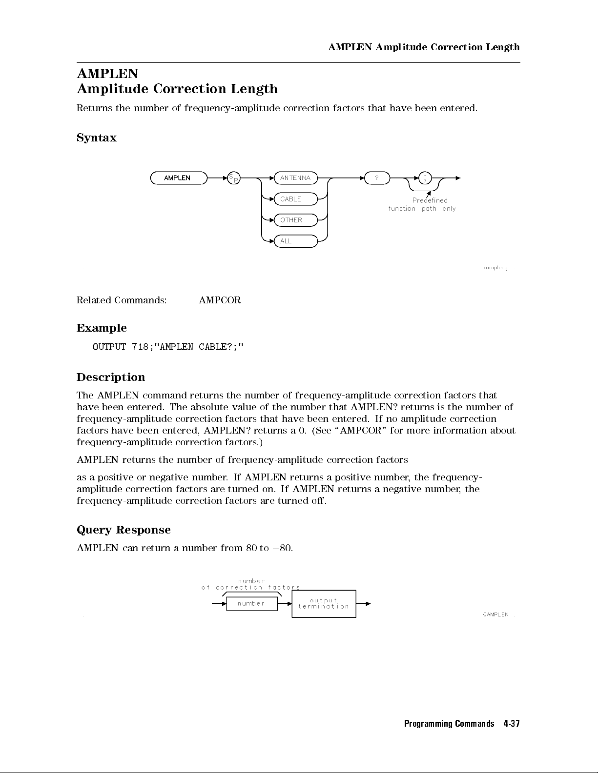
AMPLEN

Amplitude Correction Length

AMPLEN

Amplitude

Correction

Length

Returns

Syntax

Related Commands: AMPCOR

Example

Description

the number of frequency-amplitude correction factors that have been entered.

OUTPUT 718;"AMPLEN CABLE?;"

The

AMPLEN command returns the number of frequency-amplitude correction factors that

have

been entered. The absolute value of the number that AMPLEN? returns is the number of

frequency-amplitude

factors have been entered, AMPLEN? returns a 0. (See \AMPCOR" for more information about

frequency-amplitude correction factors.)

AMPLEN returns the number of frequency-amplitude correction factors

as a positive or negative number. If AMPLEN returns a positive number, the frequency-

amplitude correction factors are turned on. If AMPLEN returns a negative number, the

frequency-amplitude correction factors are turned o.

Query Response

AMPLEN can return a number from 80 to080.

correction factors that have been entered. If no amplitude correction

Programming Commands 4-37

ANNOT

Annotation

Turns

on or o the display annotation.

Syntax

NNNNNNNNNNNNNNNNNNNNNNNNNNNNNNNNNNNNNNNNNNNNNNN

Equivalent

Softkey:

ANNOTATN

ON

Preset State: ANNOT ON

Related Commands: GRAT,TITLE

Example

10

OUTPUT

20 OUTPUT 718;"ANNOT?;"

30 ENTER 718;Reply$

40

DISP

50

END

718;"ANNOT

Reply$

ON;"

Turns

Queries state of the annotation function.

Places response in a variable.

Displays response on the computer screen.

OFF

on

the

annotation.

Description

The ANNOT command turns on or o all the words and numbers (annotation) on the display

(except for the softkey labels).

Query Response

4-38 Programming Commands

APB

Trace A Plus Trace B

A

dds trace A to trace B and sends the result to trace A.

Syntax

Related Commands: CLRW, SNGLS, TS, VIEW

Example

10

20

30

40

50

OUTPUT

OUTPUT

OUTPUT

OUTPUT

OUTPUT

718;"IP;SNGLS;"

718;"TS;"

718;"VIEW

718;"TS;VIEW

TRA;RL

TRB;"

718;"APB;"

80DM;CLRW

TRB;"

60 OUTPUT 718;"BLANK TRB;VIEW TRA;"

70

END

APB

Initializes

Trace

instrument, changes to single-

A

sweep mode.

Updates the trace.

Changes

T

akes

A

ctivates

the

reference

a

measurement

APB

command.

level.

sweep

Displays the result of APB.

Plus

.

Trace

B

Description

The

APB

added

two's

command

as

16-bit

complement

adds

trace

integers

.

Negative

representation

A

to

trace B and sends the result to trace A. The traces are

numbers

of

a

are represented in two's complement format. The

negative

number is obtained by changing the 1s to 0s in

the binary representation of the number, and then binarily adding 1.

Programming Commands 4-39

ARNG

Auto Range

Enables

or disables the auto-range function.

Syntax

Equivalent Key:

Preset

Related

State:

Commands:

Example

OUTPUT

718;"ARNG ON;"

4

A

UTO

ARNG

O

VLD

RANGE

OFF

,

A

T

5

,

RL

Description

The

ARNG

instrument's

RF

attenuation

command

auto-range

or

reference

allows

function.

the

user to enable, disable, or query the current state of the

When

level

(IF step-gain) in response to either an IF or RF overload

enabled,

the auto-range function automatically adjusts

condition detected during the previous sweep.

Auto range requires overload detection capability. The RF lter section must be present (and

not in a bypass state) for RF overload detection. IF overload detection does not require the RF

lter section.

When enabled, auto range automatically enables overload detection. When disabled, auto

range does

not

disable overload detection.

Query Response

4-40 Programming Commands

A

T

Attenuation

A

T

Attenuation

Species

the RF input attenuation.

Syntax

Item Description/Default Range

Number Any real or integer. Default units are dB. Input attenuator

range of receiver.

NNNNNNNNNNNNNNNNNNNNNNNNNNNNNNNNNNNNNNNNNNN

Equivalent Softkey:

Preset

Step

State: 10 dB

Increment: in 10 dB steps

N

ATTEN AUTO MAN

Related Commands: AUTO, CPL, ML, RL

Example

OUTPUT 718;"AT 40DB;"

OUTPUT 718;"AT UP;"

Sets the attenuation to 40 dB.

Increases the attenuation to 50 dB.

Description

The AT command species the input attenuation in 10 dB steps. Normally, the input attenuator

is coupled to the reference level. When a continuous wave signal is displayed with its peak at

or below the reference level, the coupling keeps the mixer input level at or below the specied

level. The AT command allows less than the specied value at the mixer input.

When the attenuation is increased with the AT command, the reference level does not change.

If the attenuation is decreased from the coupled value using the AT command, the reference

level will be decreased. When the reference level is changed using the RL command, the

input attenuation changes to maintain a constant signal level on the display if attenuation is

auto-coupled. Using auto-couple resets the attenuation value so that a continuous wave signal

Programming Commands 4-41

A

T

Attenuation

displayed at the reference level yields010 dBm (or the specied mixer level) at the mixer

input.

The step keys, knob, and DN parameter do not allow an attenuation entry below 10 dB. Only

direct entry of \AT 0DB;" will achieve 0 dB attenuation.

CAUTION

Signal levels above +30 dBm will damage the receiver.

The CPL and UNCPL parameters allow greater control in distribution of system input

attenuation when the optional RF lter section is present in the system. At instrument preset,

the input attenuator is used exclusively to control system input attenuation when the lter

section is in either the 9 kHz to 50 MHz input path (INPUT 1), or the 20 MHz to 2.9 GHz input

path (INPUT 2).

The UNCPL parameter \uncouples" the lter section's attenuator from system control, leaving

it

at

its

system

current

attenuation

setting.

will

When

not

the lter section's attenuator has been uncoupled, changes to

change

the

setting of the lter section's input attenuator. The CPL

parameter re-establishes system control of the lter section's attenuator.

Query Response

4-42 Programming Commands

A

UNITS

Amplitude Units

A

UNITS

Amplitude

Units

Species

the amplitude units for input, output, and display.

Syntax

Equivalent Softkey:

Related

Commands:

Example

OUTPUT 718;"LN;"

OUTPUT

OUTPUT

718;"AUNITS

718;"AUNITS?;"

ENTER 718;Reply$

DISP Reply$

N

NNNNNNNNNNNNNNNNNNNNNNNNNNNNNNNNNN

Amptd Units

CAL,

DL,

MKA,

Changes instrument to linear mode.

DBMV;"

Changes

Queries

Puts response in a variable.

Displays response on the computer screen.

RL,

TH,

AMPCOR

ANTENNA,

XUNITS

the linear amplitude units to DBMV.

current

amplitude

units

.

Description

The

A

UNITS

command sets the amplitude readouts (reference level, marker, display line,

and threshold) to the specied units. Dierent amplitude units can be set for log and linear

amplitude scales.

Note

When AMPCOR antenna correction factors are ON, the current XUNITS is used.

When AMPCOR antenna correction factors are OFF

, the current A

UNITS is

used.

Programming Commands 4-43

A

UNITS

Amplitude

Units

Query Response

The query response returns the current amplitude units for the current amplitude scale.

4-44 Programming Commands