

Page 1

Agilent Technologies
8510C Network Analyzer System
Operating and Programming Manual
For use with Firmware Revision C.07.XX with CRT display
For use with Firmware Revision C.08.XX or greater with LCD
Serial Numbers
This manual applies directly to instruments with
this serial prefix number or above: 3031A.
Part Number: 08510-90281
Printed in USA
May 2001
Edition 3.0
Supersedes January 31, 1994
© Copyright Agilent Technologies 1989, 1994, 2001
Page 2

Certification
Agilent Technologies certies that this product met its publishedspecications at the time
of shipment from the factory. Agilent further certies that its calibration measurements
aretraceable to the United States National Institute of Standards and Technology, to the
extent allowed by the Institute's calibration facility, and to the calibration facilities of other
International Standards Organization members.
Warranty
This Agilent instrument product is warranted against defects in material and workmanship for
a period of one year from date of delivery. During the warranty perio d, Agilent will, at its
option, either repair or replace products which prove to be defective.
For warranty service or repair, this pro duct must b e returned to a service facility designated
by AgilentTechnologies. Buyer shall prepay shipping charges to Agilent and Agilent shall
pay shipping charges to return the product to Buyer. However, Buyer shall pay all shipping
charges, duties, and taxes for pro ducts returned to Agilen
t from another country.
Agilentwarrants that its software and rmware designated by Agilent for use with an
instrument will execute its programming instructions when properly installed on that
instrument. Agilent do es not warrant that the operation of the instrument, or software, or
rmware will be uninterrupted or error free.
Limitation of Warranty
The foregoing warranty shall not apply to defects resulting from improper or inadequate
maintenance by Buyer, Buyer-supplied software or interfacing, unauthorized modication or
misuse, operation outside of the environmental specications for the product, or improper site
preparation or maintenance.
NO OTHER WARRANTY IS EXPRESSED OR IMPLIED. AGILENT SPECIFICALLY DISCLAIMS THE
IMPLIED WARRANTIES OF MERCHANTABILITY AND FITNESS FOR A PARTICULAR PURPOSE.
EXCLUSIVE REMEDIES
THE REMEDIES PROVIDED HEREIN ARE BUYER'S SOLE AND EXCLUSIVE REMEDIES. Agilent SHALL
NOT BE LIABLE FOR ANY DIRECT, INDIRECT, SPECIAL, INCIDENTAL, OR CONSEQUENTIAL
DAMAGES, WHETHER BASED ON CONTRACT, TORT, OR ANY OTHER LEGAL THEORY.
c
Copyright AgilentTechnologies, Inc., 1989, 1994, 2001 All rights reserved. 1400
FountaingroveParkway, Santa Rosa, CA 95403 U.S.A.
Page 3

Safety and Regulatory Information
Review this product and related documentation to familiarize yourself with safety markings
and instructions before you operate this instrument.
This product has been designed and tested in accordance with the standards listed on the
Manufacturer's Declaration of Conformity, and has been supplied in a safe condition. The
documentation contains information and warnings that must be followed by the user to ensure
safe operation and to maintain the pro duct in a safe condition.
Caution
Warning
The CAUTION notice denotes a hazard. It calls attention to a pro cedure
which, if not correctly p erformed or adhered to, could result in damage to or
destruction of the instrument. Do not pro ceed beyond a
caution
sign until the
indicated conditions are fully understood and met.
The WARNING notice denotes a hazard. It calls attention to a procedure which,
if not correctly performed or adhered to, could result in injury or loss of life. Do
not proceed beyondaWARNING sign until the indicated conditions are fully
understood and met.
When you see this symbol on your instrument, you should refer to the
instrument's instruction manual for important information.
The CSA mark is the Canadian Standards Association safet
The CE mark is a registered trademark of the European Communit
y mark.
y.Ifitis
accompanied byayear, it indicates the year the design was proven.
This symbol indicates that the instrument requires alternating current (ac) input.
This symbol is used to mark the STANDBY/OFF position of the power line
switch.
This symbol is used to mark the ON position of the p o
wer line switch.
This text indicates that the instrument is an industrial Scientic and Medical
Group 1 Class A product (CISPER 11, Clause 4).
The C-tick mark is a registered trademark of the Sp ectrum Management Agency
of Australia. This signies compliance with the Australian EMC Framework
regulations under the terms of Radio communications Act of 1992.
iii
Page 4

General Safety Considerations
Warning
Caution
This is a Safety Class 1 Product (provided with a protective earthing ground
incorporated in the power cord). The mains plug shall only be inserted in a
socket outlet provided with a protective earth contact. Any interruption of the
protective conductor inside or outside of the product is likely to make the
product dangerous. Intentional interruption is prohibited.
Before applying power, verify that the product is configured to match the
available main power source as described in the input power configuration
instructions. If this product is to be powered by autotransformer, make sure
the common terminal is connected to the neutral (grounded) side of the ac
power supply.
If this product is not used as specified, the protection provided by the
equipment could be impaired. This product must be used in a normal
condition (in which all means for protection are intact) only.
Always use the three-prong ACpower cord supplied with this product.
Failure to ensure adequate earth grounding by not using this cord may cause
product damage.
Ventilation Requirements: When installing the product in a cabinet, the
convection into and out of the product must not be restricted. The ambient
temperature (outside the cabinet) must not be restricted. The ambient
temperature (outside the cabinet) must be less than the maximum op erating
temperature of the product by4
for every 100 watts dissipated in the
cabinet. If the total power dissipated in the cabinet is greater than 800
watts forced convection must be used.
This product is designed for use in Installation Category II and P
Degree 2 per IEC 1010 and 664 respectiv
ely.
ollution
iv
Page 5

Acoustic Noise Emissions Declaration
This is to declare that this instrument is in conformance with the German Regulation on
Noise Declaration for Machines (Laermangab e nach der Maschinenlaermrerordnung03.
GSGV Deutschland).
Acoustic Noise Emission/Geraeuschemission
LpA<70 dB LpA<70 dB
Operator p osition am Arbeitsplatz
normal operation normaler Betrieb
Per ISO 7779 nach DIN 45635 t. 19
By internet, phone, or fax, get assistance with all your test & measurement needs.
Table 0-1. Contacting Agilent
Online Assistance:
United States
(tel) 1 800 452 4844
www.agilent.com/find/assist
Japan
(tel) (81) 426 56 7832
(fax) (81) 426 56 7840
New Zealand
(tel) 0 800 738 378
(fax) 64 4 495 8950
Canada
(tel) 1 877 894 4414
(fax) (905) 206 4120
Europe
(tel) (31 20) 547 2323
(fax) (31 20) 547 2390
Latin America
(tel) (305) 269 7500
(fax) (305) 269 7599
Australia
(tel) 1 800 629 485
(fax) (61 3) 9210 5947
Asia Pacic
(tel) (852) 3197 7777
(fax) (852) 2506 9284
v
Page 6

Introduction
This
8510C Operating and Programming Manual
comprehensive tutorial material to help you learn typical applications and op erating details of
the Agilent 8510 network analyzer system.
is designed to provide you with
A companion volume, the
8510 front-panel hardkeys, menu softkeys, and programming mnemonics. Eachentry also
includes information about how to use the function in programmed op eration.
Note
Note
The original 8510C incorporated a cathode ray tube (CRT) based display. The
current design incorp orates a liquid crystal display (LCD). In this manual
references to either CRT or LCD apply to both display designs unless noted
otherwise.
Systems with a CRT based display in the 85101C use rmware revision
C.07.XX or greater.
Systems with an LCD require rmware revision C.08.00 or greater.
In this manual, the terms GPIB (General Purpose Interface Bus) and
HP-IB (Hewlett-Packard Interface Bus) refer to the same proto col.
Instrument softkeys for HP-IB related functions use \HP-IB", for example,
NNNNNNNNNNNNNNNNNNNNNNNNNNNNNNNNNNNNNNNNNNNNNNN
HP-IB ADDRESSES
8510 Keyword Dictionary
NNNNNNNNNNNNNNNNNNNNNNNNNNNNNNNNNNNNNNNNNNNNNNN
or
HP-IB CONFIGURE
provides a complete alphab etical list of
.
vi
Page 7

vii
Page 8

Typeface Conventions
The following conventions are used in the
Keyword Dictionary
Italics
Italic type is used for emphasis, and for titles of manuals and other publications. It is also
used to designate a variable entry value.
Computer
Computer type is used for information displayed on the instrument and to designate a
programming command or series of commands.
4
Hardkeys
Instrumentkeys are represented in \key cap." You are instructed to
W
WWWWWWWWWWWWWWWWWWWWWWWWWWW
Softkeys
Softkeys are located along side of the displa
display. These keys are represented in \softkey." You are instructed to
5
.
8510C Operating and Programming Manual
press
a hardkey.
y, and their functions depend on the current
select
a softkey.
and the
viii
Page 9

DECLARATION OF CONFORMITY
According to ISO/IEC Guide 22 and CEN/CENELEC EN 45014
Manufacturer’s Name: Agilent Technologies, Inc.
Manufacturer’s Address: 1400 Fountaingrove Parkway
Santa Rosa, CA 95403-1799
USA
Declares that the product:
Product Name: Network Analyzer
Model Number: 8510C
Product Options: This declaration covers all options of the above product.
Conforms to the following product specifications:
EMC: IEC 61326-1:1997+A1:1998 / EN 61326-1:1997+A1:1998
CISPR 11:1990 / EN 55011-1991 (Group 1, Class A)
IEC 61000-4-2:1995+A1998 / EN 61000-4-2:1995 (4 kV CD, 8 kV AD)
IEC 61000-4-3:1995 / EN 61000-4-3:1995 (3 V/m, 80 - 1000 MHz)
IEC 61000-4-4:1995 / EN 61000-4-4:1995 (0.5 kV sig. lines, 1 kV power lines)
IEC 61000-4-5:1995 / EN 61000-4-5:1996 (0.5 kV L-L, 1 kV L-G)
IEC 61000-4-6:1996 / EN 61000-4-6:1998 (3 V, 0.15 – 80 MHz)
IEC 61000-4-11:1994 / EN 61000-4-11:1998 (1 cycle, 100%)
Safety: IEC 61010-1:1990 + A1:1992 + A2:1995 / EN 61010-1:1993 +A2:1995
CAN/CSA-C22.2 No. 1010.1-92
Supplementary Information:
The product herewith complies with the requirements of the Low Voltage Directive 73/23/EEC and the
EMC Directive 89/336/EEC and carries the CE-marking accordingly.
Santa Rosa, CA, USA 28 February, 2001
Greg Pfeiffer/Quality Engineering Manager
For further information, please contact your local Agilent Technologies sales office, agent or distributor.
Page 10

Contents
1. Introduction to the 8510C Network Analyzer System
Introduction . . . . . . . . . . . . . . . . . . . . . . . . . . . . . 1-1
8510 Network Analyzer System Description . . . . . . . . . . . . . . 1-1
FrontPanel Controls . . . . . . . . . . . . . . . . . . . . . . . . 1-2
Display Modes and Annotation Areas . . . . . . . . . . . . . . . . . . 1-3
Channel/Parameter Identication Area . . . . . . . . . . . . . . . . 1-4
Stimulus Values Area . . . . . . . . . . . . . . . . . . . . . . . . 1-4
ActiveEntry Area . . . . . . . . . . . . . . . . . . . . . . . . . 1-5
Knowing When a Function Is Selected . . . . . . . . . . . . . . . . 1-5
Recognizing Mutually-Exclusive Functions . . . . . . . . . . . . . . 1-5
Title Area . . . . . . . . . . . . . . . . . . . . . . . . . . . . . 1-5
System Messages Area . . . . . . . . . . . . . . . . . . . . . . . . 1-5
Enhancement Annotation Area . . . . . . . . . . . . . . . . . . . . 1-6
Softkey Menu and Marker List Display Area . . . . . . . . . . . . . . 1-6
Using ENTRY Blo ck Keys . . . . . . . . . . . . . . . . . . . . . . . 1-7
Uparrow(
4
5
) and Downarrow(
8
4
5
) Keys . . . . . . . . . . . . . . . 1-7
9
Using Numeric Keys . . . . . . . . . . . . . . . . . . . . . . . . . 1-7
Using Units Terminator Keys . . . . . . . . . . . . . . . . . . . . . 1-8
Using the Prior Menu Key . . . . . . . . . . . . . . . . . . . . . 1-8
Using the Backspace Key . . . . . . . . . . . . . . . . . . . . . 1-8
Using the
4
=MARKER
5
Key . . . . . . . . . . . . . . . . . . . . . 1-8
Using ACTIVE CHANNEL Block Keys . . . . . . . . . . . . . . . . . 1-9
Coupling Channels . . . . . . . . . . . . . . . . . . . . . . . . . 1-9
Coupling Conditions . . . . . . . . . . . . . . . . . . . . . . . . 1-10
Using MENUS Block Keys . . . . . . . . . . . . . . . . . . . . . . . 1-10
Using STIMULUS, PARAMETER, FORMAT, and RESPONSE Blocks Keys . 1-11
Using INSTRUMENT STATE Keys . . . . . . . . . . . . . . . . . . . 1-12
Using AUXILIARY MODE Keys . . . . . . . . . . . . . . . . . . . . 1-12
Using MEASUREMENT Block Key . . . . . . . . . . . . . . . . . . . 1-12
Using the Menus, Examples . . . . . . . . . . . . . . . . . . . . . . 1-13
To Create, Edit, or Delete a Title . . . . . . . . . . . . . . . . . . . 1-13
To Adjust the Date/Time Clo ck . . . . . . . . . . . . . . . . . . . 1-13
The Analyzer Remembers Previous Settings (Limited Instrument State) . 1-14
INSTRUMENT STATE Blo ck . . . . . . . . . . . . . . . . . . . . 1-15
4
USER PRESET
5
Key . . . . . . . . . . . . . . . . . . . . . . . . . . 1-15
Saving and Recalling Complete Instrument States . . . . . . . . . . . 1-15
4
5
LOCAL
Key . . . . . . . . . . . . . . . . . . . . . . . . . . . 1-16
1
Page 11

2. Introductory Measurement Sequence
Introduction . . . . . . . . . . . . . . . . . . . . . . . . . . . . . 2-1
Verifying the System Setup . . . . . . . . . . . . . . . . . . . . . . 2-1
If some instruments do not resp ond at power-up . . . . . . . . . . . 2-2
Turning on system power, the sequence . . . . . . . . . . . . . . . 2-2
Waiting for self-test and initialization . . . . . . . . . . . . . . . . 2-3
Measurement Sequence Example 1: Frequency Domain Measurement . . . . 2-3
1. Setting Up the Measurement. . . . . . . . . . . . . . . . . . . . 2-4
Making Connections . . . . . . . . . . . . . . . . . . . . . . . . 2-4
Factory Preset State . . . . . . . . . . . . . . . . . . . . . . . 2-5
Set Stimulus, Parameter, Format, Response . . . . . . . . . . . . . 2-5
2. Performing the Measurement Calibration . . . . . . . . . . . . . . 2-7
Making a reection frequency response calibration . . . . . . . . . . 2-7
To Identify, Create, and Store S11Measurement Calibration Data . . . 2-7
Reading the displayed response . . . . . . . . . . . . . . . . . . 2-8
Making a transmission frequency response calibration . . . . . . . . . 2-8
To Identify, Create, and Store S21Measurement Calibration Data . . . 2-8
3. Making a Measurement . . . . . . . . . . . . . . . . . . . . . . 2-9
To measure return loss (S11) in LOG MAG format (frequency domain
measurements) . . . . . . . . . . . . . . . . . . . . . . . . 2-9
To measure the insertion loss (S
4. Saving Data and Getting an Output of the Results
) in LOG MAG format . . . . . . . . 2-10
21
. . . . . . . . . . 2-11
Plotting Advantages . . . . . . . . . . . . . . . . . . . . . . . . 2-11
To set up the plotter . . . . . . . . . . . . . . . . . . . . . . . 2-11
Plotting the Current Display . . . . . . . . . . . . . . . . . . . . 2-12
To plot selected areas of the results display. . . . . . . . . . . . . . 2-12
Measurement Sequence Example 2: Time Domain . . . . . . . . . . . . . 2-13
3. Principles of Operation
Introduction . . . . . . . . . . . . . . . . . . . . . . . . . . . . . 3-1
Basic Principles of Network Measurements . . . . . . . . . . . . . . . . 3-1
System Block Diagram . . . . . . . . . . . . . . . . . . . . . . . 3-3
Description of the 8510 Network Analyzer . . . . . . . . . . . . . . . 3-3
How the 8510 Makes Measurements . . . . . . . . . . . . . . . . . 3-4
Test and Measurement Input Channels . . . . . . . . . . . . . . . 3-4
Ratio Measurements and Sampling Details . . . . . . . . . . . . . . 3-4
Digital Signal Processing . . . . . . . . . . . . . . . . . . . . . . . 3-5
CPU and Memory Description . . . . . . . . . . . . . . . . . . . 3-5
Data Processing Steps . . . . . . . . . . . . . . . . . . . . . . . 3-5
Button Push Detection . . . . . . . . . . . . . . . . . . . . . . . 3-6
Test Signal Sources . . . . . . . . . . . . . . . . . . . . . . . . . 3-6
Sources in ramp-sweep mode . . . . . . . . . . . . . . . . . . . . 3-7
Sources in step-sweep mo de . . . . . . . . . . . . . . . . . . . . 3-7
Test Sets . . . . . . . . . . . . . . . . . . . . . . . . . . . . . . 3-7
Coaxial Test Set Information . . . . . . . . . . . . . . . . . . . . 3-7
Reection/Transmission Test Sets . . . . . . . . . . . . . . . . . . 3-8
S-Parameter Test Sets . . . . . . . . . . . . . . . . . . . . . . . 3-9
Customized Test Sets . . . . . . . . . . . . . . . . . . . . . . . 3-10
Measurement Accessories . . . . . . . . . . . . . . . . . . . . . . 3-11
Source Output-to-Test-Set Input Signal Cable . . . . . . . . . . . . 3-11
Test Port Return Cables . . . . . . . . . . . . . . . . . . . . . . 3-11
2
Page 12

Extension Lines . . . . . . . . . . . . . . . . . . . . . . . . . . 3-11
Adapters (To Protect Test Ports from Wear) . . . . . . . . . . . . . 3-13
Proper Connector Care and Use . . . . . . . . . . . . . . . . . . 3-13
Calibration Kits . . . . . . . . . . . . . . . . . . . . . . . . . . 3-13
Verication Kits . . . . . . . . . . . . . . . . . . . . . . . . . . 3-14
Automatic Recall of Instrument Settings . . . . . . . . . . . . . . . . . 3-15
The Added Benet of the SAVE/RECALL Feature . . . . . . . . . . . 3-15
Factory Preset State . . . . . . . . . . . . . . . . . . . . . . . . 3-16
Hardware State . . . . . . . . . . . . . . . . . . . . . . . . . . . . 3-17
4. Measurement Controls
Display . . . . . . . . . . . . . . . . . . . . . . . . . . . . . . . 4-1
Display Modes . . . . . . . . . . . . . . . . . . . . . . . . . . . 4-2
Dual Channel Display Modes . . . . . . . . . . . . . . . . . . . . 4-3
Single Channel, Four Parameter Display Modes . . . . . . . . . . . . 4-5
Adjust Display Menu . . . . . . . . . . . . . . . . . . . . . . . . . 4-5
Intensity. . . . . . . . . . . . . . . . . . . . . . . . . . . . . . 4-5
Background Intensity (CRT only) . . . . . . . . . . . . . . . . . . . 4-6
Modify colors . . . . . . . . . . . . . . . . . . . . . . . . . . . . 4-6
Default Colors . . . . . . . . . . . . . . . . . . . . . . . . . . 4-8
External Video (CRT only) . . . . . . . . . . . . . . . . . . . . . 4-9
External Video (LCD only) . . . . . . . . . . . . . . . . . . . . . 4-10
Limits: Limit Lines and Limit Points Measurements . . . . . . . . . . . . 4-11
Types of Limits . . . . . . . . . . . . . . . . . . . . . . . . . . . 4-11
Limit Testing . . . . . . . . . . . . . . . . . . . . . . . . . . . . 4-11
Limit Tables . . . . . . . . . . . . . . . . . . . . . . . . . . . . 4-12
Creating a Limit Test . . . . . . . . . . . . . . . . . . . . . . . . 4-12
To Set Up the Measurement . . . . . . . . . . . . . . . . . . . . 4-12
To Set the Limit Test Values . . . . . . . . . . . . . . . . . . . . 4-13
To Dene the Maximum Limit . . . . . . . . . . . . . . . . . . . 4-13
To Dene Minimum Limit Lines . . . . . . . . . . . . . . . . . . 4-15
Editing Limits in the Limits Table . . . . . . . . . . . . . . . . . . 4-16
Trace Memory Op erations . . . . . . . . . . . . . . . . . . . . . . . 4-17
Storing Trace Data in Memory . . . . . . . . . . . . . . . . . . . . 4-17
To Display a Stored Trace . . . . . . . . . . . . . . . . . . . . . 4-17
Settings that can and cannot b e changed . . . . . . . . . . . . . . 4-17
To Display Data and Memory Simultaneously . . . . . . . . . . . . 4-17
Settings that can and cannot b e changed . . . . . . . . . . . . . . 4-17
To Select the Default Memory . . . . . . . . . . . . . . . . . . . 4-18
Which memory lo cations are volatile, which are not . . . . . . . . . 4-20
What is the operational life of non-volatile memory . . . . . . . . . 4-20
Trace Math Operations . . . . . . . . . . . . . . . . . . . . . . . 4-20
Data from Channel 1 and Data from Channel 2 . . . . . . . . . . . . . 4-22
Domain . . . . . . . . . . . . . . . . . . . . . . . . . . . . . . . 4-23
Automatic Memory of Domain Settings . . . . . . . . . . . . . . . . 4-24
Applicable Calibration Types for Each Domain Mo de . . . . . . . . . . 4-24
Auxiliary Voltage Domain Example . . . . . . . . . . . . . . . . . . 4-24
FORMAT . . . . . . . . . . . . . . . . . . . . . . . . . . . . . . 4-25
Cartesian Formats . . . . . . . . . . . . . . . . . . . . . . . . . 4-25
Smith Chart Formats . . . . . . . . . . . . . . . . . . . . . . . . 4-25
Polar Display Formats . . . . . . . . . . . . . . . . . . . . . . . . 4-25
3
Page 13

Format Keys Available on the FrontPanel . . . . . . . . . . . . . . . 4-25
Markers . . . . . . . . . . . . . . . . . . . . . . . . . . . . . . . 4-29
Using the Markers . . . . . . . . . . . . . . . . . . . . . . . . . 4-29
Select the Active Marker . . . . . . . . . . . . . . . . . . . . . . 4-29
Marker Units . . . . . . . . . . . . . . . . . . . . . . . . . . . 4-30
Continuous and Discrete . . . . . . . . . . . . . . . . . . . . . . 4-31
Marker List Displays . . . . . . . . . . . . . . . . . . . . . . . 4-31
Delta Mode Markers . . . . . . . . . . . . . . . . . . . . . . . . 4-33
Marker Search Modes . . . . . . . . . . . . . . . . . . . . . . . . 4-34
Search Right and Search Left . . . . . . . . . . . . . . . . . . . . 4-35
Delta Mode Operation . . . . . . . . . . . . . . . . . . . . . . . 4-36
Marker Familiarization Sequence . . . . . . . . . . . . . . . . . . . 4-36
Parameter . . . . . . . . . . . . . . . . . . . . . . . . . . . . . . 4-38
Basic Parameters . . . . . . . . . . . . . . . . . . . . . . . . . . 4-38
S-Parameter Denitions and Conventions . . . . . . . . . . . . . . . 4-38
Parameter Menu . . . . . . . . . . . . . . . . . . . . . . . . . . 4-39
User Parameters . . . . . . . . . . . . . . . . . . . . . . . . . 4-40
Redene Parameter . . . . . . . . . . . . . . . . . . . . . . . . 4-41
Redene Basic Parameters . . . . . . . . . . . . . . . . . . . . . 4-42
Redene User Parameters . . . . . . . . . . . . . . . . . . . . . 4-44
Measuring Power (dBm) . . . . . . . . . . . . . . . . . . . . . . . 4-44
Dynamic Range Considerations . . . . . . . . . . . . . . . . . . . . 4-46
Response . . . . . . . . . . . . . . . . . . . . . . . . . . . . . . 4-48
Changing Display Scale and Reference . . . . . . . . . . . . . . . . . 4-48
Setting Scale and Reference Values Automatically . . . . . . . . . . . 4-48
Changing Display Scale Manually . . . . . . . . . . . . . . . . . . 4-48
Changing the Position of the Reference Line Manually . . . . . . . . . 4-48
Changing the Value of the Reference Line Manually . . . . . . . . . . 4-49
Automatic Recall of Previous Display Settings . . . . . . . . . . . . 4-49
Hierarchy of the Automatic Memory . . . . . . . . . . . . . . . . 4-49
The automatic memory does not include Stim
ulus settings . . . . . . 4-50
Other options for control of Stimulus settings . . . . . . . . . . . . 4-50
The Eect of Factory Preset on Display Settings . . . . . . . . . . . 4-50
Response Menu. . . . . . . . . . . . . . . . . . . . . . . . . . . 4-50
Trace Averaging and Smoothing . . . . . . . . . . . . . . . . . . . 4-50
Averaging . . . . . . . . . . . . . . . . . . . . . . . . . . . . 4-51
Averaging Details . . . . . . . . . . . . . . . . . . . . . . . . . 4-51
Notication when averaging is nished . . . . . . . . . . . . . . . 4-51
Averaging Factor Recommendations . . . . . . . . . . . . . . . . . 4-51
Smoothing . . . . . . . . . . . . . . . . . . . . . . . . . . . . 4-52
Electrical Delay. . . . . . . . . . . . . . . . . . . . . . . . . . . 4-53
Using Electrical Delay. . . . . . . . . . . . . . . . . . . . . . . 4-53
DelayFeatures . . . . . . . . . . . . . . . . . . . . . . . . . . 4-53
Coaxial Delay . . . . . . . . . . . . . . . . . . . . . . . . . 4-54
Waveguide Delay . . . . . . . . . . . . . . . . . . . . . . . . 4-54
Table Delay . . . . . . . . . . . . . . . . . . . . . . . . . . 4-54
Selecting Velo cityFactor . . . . . . . . . . . . . . . . . . . . . 4-54
Auto Delay . . . . . . . . . . . . . . . . . . . . . . . . . . . . 4-54
Phase Oset . . . . . . . . . . . . . . . . . . . . . . . . . . . . 4-54
Magnitude Slope and Magnitude Oset . . . . . . . . . . . . . . . . 4-55
Stimulus . . . . . . . . . . . . . . . . . . . . . . . . . . . . . . . 4-56
4
Page 14

Set Frequency Sweep . . . . . . . . . . . . . . . . . . . . . . . . 4-56
Set Sweep Using Markers . . . . . . . . . . . . . . . . . . . . . . 4-57
Set Stimulus Power . . . . . . . . . . . . . . . . . . . . . . . . . 4-57
Setting and Monitoring Signal Levels . . . . . . . . . . . . . . . . 4-57
Set Source RF Output Level . . . . . . . . . . . . . . . . . . . 4-58
Power Slop e On/O . . . . . . . . . . . . . . . . . . . . . . . 4-59
Attenuator Port: 1 and Attenuator Port: 2 . . . . . . . . . . . . . 4-59
Setting power for passive devices, or devices with gain . . . . . . . . 4-59
Source Power and Flatness Correction Calibration . . . . . . . . . . . 4-60
Selecting the Number of Points to Measure . . . . . . . . . . . . . . . 4-61
Source Sweep Mo des . . . . . . . . . . . . . . . . . . . . . . . . 4-62
Speed of Step and Frequency vs. Ramp Modes . . . . . . . . . . . . 4-63
Measurement Hint . . . . . . . . . . . . . . . . . . . . . . . . 4-63
Entering Ramp, Step, and Single Point Stimulus Values . . . . . . . . 4-63
Sweep Time . . . . . . . . . . . . . . . . . . . . . . . . . . . . 4-64
Example: Eects of Sweep Time . . . . . . . . . . . . . . . . . . . 4-64
Sweep Execution, Hold/Single/Numb er of Groups/Continual . . . . . . . 4-65
Why Use Number of Groups? . . . . . . . . . . . . . . . . . . . . 4-66
Coupled/Uncoupled Channels . . . . . . . . . . . . . . . . . . . 4-66
How to tell if a function is coupled . . . . . . . . . . . . . . . . 4-67
Dual Channel . . . . . . . . . . . . . . . . . . . . . . . . . . 4-67
Uncoupled Stimulus Settings and Dual Channel Displays . . . . . . . 4-67
Trigger Mo des . . . . . . . . . . . . . . . . . . . . . . . . . . 4-68
Creating a Frequency List . . . . . . . . . . . . . . . . . . . . . . 4-69
Entering the First Segment. . . . . . . . . . . . . . . . . . . . . 4-69
Add Segments . . . . . . . . . . . . . . . . . . . . . . . . . . 4-70
Editing the Frequency List . . . . . . . . . . . . . . . . . . . . . 4-70
Changing a Segment . . . . . . . . . . . . . . . . . . . . . . 4-70
Deleting a Segment . . . . . . . . . . . . . . . . . . . . . . . 4-71
Adding a Segment . . . . . . . . . . . . . . . . . . . . . . . 4-71
To Duplicate Points . . . . . . . . . . . . . . . . . . . . . . . . 4-71
Frequency List Save and Recall . . . . . . . . . . . . . . . . . . . 4-71
Selecting All Segments or a Single Segment. . . . . . . . . . . . . 4-71
To Exit Frequency List . . . . . . . . . . . . . . . . . . . . . . 4-72
5. Using System Functions
Chapter Contents . . . . . . . . . . . . . . . . . . . . . . . . . . . 5-1
System Menus . . . . . . . . . . . . . . . . . . . . . . . . . . . . 5-2
Controls that Aect the Network Analyzer . . . . . . . . . . . . . . . . 5-3
Phaselock Controls . . . . . . . . . . . . . . . . . . . . . . . . . 5-3
LockType . . . . . . . . . . . . . . . . . . . . . . . . . . . . 5-3
Step Type . . . . . . . . . . . . . . . . . . . . . . . . . . . . 5-3
Normal Step . . . . . . . . . . . . . . . . . . . . . . . . . . 5-4
Quick Step Mode . . . . . . . . . . . . . . . . . . . . . . . . 5-4
Lock Speed . . . . . . . . . . . . . . . . . . . . . . . . . . . 5-4
Warning Beeper . . . . . . . . . . . . . . . . . . . . . . . . . . 5-5
IF Calibration and Correction . . . . . . . . . . . . . . . . . . . . 5-5
IF Calibration Controls . . . . . . . . . . . . . . . . . . . . . . 5-5
DisplayFunctions . . . . . . . . . . . . . . . . . . . . . . . . . . 5-5
Creating a Title . . . . . . . . . . . . . . . . . . . . . . . . . 5-5
Deleting a Title . . . . . . . . . . . . . . . . . . . . . . . . . . 5-6
5
Page 15

Adjusting the Date/Time Clock . . . . . . . . . . . . . . . . . . 5-6
Using SecurityFeatures in the System
NNNNNNNNNNNNNNNNNNNNNNNNNNNNNNNNNNNNNNNNNNNNNNNNNNNNN
DISPLAY FUNCTIONS
Menu . . . 5-7
Controls that Aect Input/Output . . . . . . . . . . . . . . . . . . . 5-8
GPIB Addresses . . . . . . . . . . . . . . . . . . . . . . . . . . 5-8
GPIB Congure . . . . . . . . . . . . . . . . . . . . . . . . . . 5-9
Edit Multiple Source . . . . . . . . . . . . . . . . . . . . . . . . 5-9
Power Leveling . . . . . . . . . . . . . . . . . . . . . . . . . . . 5-9
Controlling Multiple Sources . . . . . . . . . . . . . . . . . . . . . . 5-11
Using the Multiple Source Menu . . . . . . . . . . . . . . . . . . . 5-12
HowtoEnter the Example Conguration . . . . . . . . . . . . . . 5-13
Nowsave the conguration . . . . . . . . . . . . . . . . . . . . 5-14
Millimeter Wave Mixers . . . . . . . . . . . . . . . . . . . . . . 5-15
Uses for the SOURCE 1 and RECEIVER Formulas . . . . . . . . . . . 5-15
SOURCE 1 Formula Use . . . . . . . . . . . . . . . . . . . . . . 5-15
Receiver Formula Use . . . . . . . . . . . . . . . . . . . . . . . 5-15
Why are these settings used? . . . . . . . . . . . . . . . . . . . 5-16
Service Functions . . . . . . . . . . . . . . . . . . . . . . . . . . . 5-18
Test Menu . . . . . . . . . . . . . . . . . . . . . . . . . . . . . 5-18
Disc Commands . . . . . . . . . . . . . . . . . . . . . . . . . 5-19
System Bus Softkeys . . . . . . . . . . . . . . . . . . . . . . . . 5-19
IF Gain . . . . . . . . . . . . . . . . . . . . . . . . . . . . . . 5-20
Why Use Manual Control . . . . . . . . . . . . . . . . . . . . . 5-20
Why the problem o ccurs . . . . . . . . . . . . . . . . . . . . . 5-20
How to Use Manual IF Gain Controls Properly . . . . . . . . . . . . 5-22
Peek and Poke . . . . . . . . . . . . . . . . . . . . . . . . . . . 5-23
Purpose of Peek and Poke . . . . . . . . . . . . . . . . . . . . . 5-23
6. COPY Printing and Plotting
Chapter Contents . . . . . . . . . . . . . . . . . . . . . . . . . . . 6-1
Installation Considerations . . . . . . . . . . . . . . . . . . . . . . . 6-2
Supported Interfaces . . . . . . . . . . . . . . . . . . . . . . . . 6-2
Connecting a GPIB Printer or Plotter . . . . . . . . . . . . . . . . . 6-2
Connecting an RS-232 Printer or Plotter . . . . . . . . . . . . . . . . 6-2
Selecting the GPIB (System Bus) or RS-232 Ports . . . . . . . . . . . 6-2
RS-232 Print/Plot Buers . . . . . . . . . . . . . . . . . . . . . . . 6-3
Adding Custom Annotations to the Screen . . . . . . . . . . . . . . . . 6-3
Using a Printer . . . . . . . . . . . . . . . . . . . . . . . . . . . . 6-4
Printing Features . . . . . . . . . . . . . . . . . . . . . . . . . . 6-4
What Is Printed? . . . . . . . . . . . . . . . . . . . . . . . . . . 6-4
Installing a Printer . . . . . . . . . . . . . . . . . . . . . . . . . 6-4
Selecting the Output Port . . . . . . . . . . . . . . . . . . . . . . 6-4
Printer and the 8510C Conguration . . . . . . . . . . . . . . . . . . 6-5
Using a Laser Printer . . . . . . . . . . . . . . . . . . . . . . . . . 6-6
Conguring the Laser Printer . . . . . . . . . . . . . . . . . . . . . 6-6
Using the Standard Conguration . . . . . . . . . . . . . . . . . . . 6-6
Using Other Laser Printer Settings . . . . . . . . . . . . . . . . . 6-6
Conguring the Network Analyzer . . . . . . . . . . . . . . . . . 6-6
Selecting Printer Resolution . . . . . . . . . . . . . . . . . . . . 6-6
Using the High Speed Conguration . . . . . . . . . . . . . . . . . . 6-7
Why is it faster? . . . . . . . . . . . . . . . . . . . . . . . . . 6-7
6
Page 16

My printer has built-in HP-GL. Do I still need the cartridge? . . . . . . 6-7
Ordering the Cartridge . . . . . . . . . . . . . . . . . . . . . . 6-7
Having Enough Printer Memory . . . . . . . . . . . . . . . . . . 6-8
Setting the Printer Up . . . . . . . . . . . . . . . . . . . . . . . 6-8
Using Other Laser Printer Settings . . . . . . . . . . . . . . . . . 6-8
Conguring the Network Analyzer . . . . . . . . . . . . . . . . . 6-8
Switching Between Real Plotters and HP-GL-emulating Laser Printers . . 6-9
Using an HP DeskJet, DeskJet Plus, or DeskJet 500 or 550 Series Printer . . 6-10
Using Serial Setup . . . . . . . . . . . . . . . . . . . . . . . . . 6-10
Setting the Serial DIP Switch . . . . . . . . . . . . . . . . . . . 6-10
Preparing the Printer for Use . . . . . . . . . . . . . . . . . . . . 6-10
Conguring the Network Analyzer . . . . . . . . . . . . . . . . . . 6-10
Selecting Printer Resolution . . . . . . . . . . . . . . . . . . . . 6-10
Using the HP DeskJet 500C or 550C Additional Steps Required . . . . 6-10
Using an HP QuietJet, QuietJet Plus, PaintJet, or PaintJet XL Printer . . . 6-11
Using Serial Setup . . . . . . . . . . . . . . . . . . . . . . . . . 6-11
Setting the Serial DIP Switch . . . . . . . . . . . . . . . . . . . 6-11
Setting Up GPIB . . . . . . . . . . . . . . . . . . . . . . . . . . 6-12
Setting the GPIB Address DIP Switch. . . . . . . . . . . . . . . . 6-12
Preparing the Printer for Use . . . . . . . . . . . . . . . . . . . . . 6-12
Conguring the Network Analyzer . . . . . . . . . . . . . . . . . . 6-12
Selecting Printer Resolution (HP QuietJet and QuietJet Plus Printers) . 6-12
Selecting Printer Resolution (HP PaintJet and PaintJet XL Printers) . . 6-13
Printing In Color . . . . . . . . . . . . . . . . . . . . . . . . . 6-13
Using an HP ThinkJet Printer . . . . . . . . . . . . . . . . . . . . . 6-13
Using Serial Setup . . . . . . . . . . . . . . . . . . . . . . . . . 6-13
Setting the Serial DIP Switch . . . . . . . . . . . . . . . . . . . 6-13
Setting Up for GPIB . . . . . . . . . . . . . . . . . . . . . . . . 6-13
Setting the GPIB Address DIP Switch. . . . . . . . . . . . . . . . 6-13
Preparing the Printer for Use . . . . . . . . . . . . . . . . . . . . 6-14
Conguring the Network Analyzer . . . . . . . . . . . . . . . . . . 6-14
Selecting Printer Resolution . . . . . . . . . . . . . . . . . . . . 6-14
Using Non-HP Printers . . . . . . . . . . . . . . . . . . . . . . . . 6-15
Using Serial Setup . . . . . . . . . . . . . . . . . . . . . . . . . 6-15
Setting the Serial DIP Switch . . . . . . . . . . . . . . . . . . . 6-15
Setting Up for GPIB . . . . . . . . . . . . . . . . . . . . . . . . 6-15
Setting the GPIB Address DIP Switch. . . . . . . . . . . . . . . . 6-15
Pre-Printing Check-Out . . . . . . . . . . . . . . . . . . . . . . . 6-15
Printing . . . . . . . . . . . . . . . . . . . . . . . . . . . . . . . 6-16
Printing Orientation: Either Landscape or Portrait . . . . . . . . . . . 6-16
Printing One Snapshot p er Page (Portrait or Landscape) . . . . . . . . . 6-17
Printing Two Snapshots per Page . . . . . . . . . . . . . . . . . . . 6-17
Printing Tabular Measurement Data . . . . . . . . . . . . . . . . . 6-18
Changing the Tabular Data Format . . . . . . . . . . . . . . . . . 6-19
Printing Instrument Settings and System Conguration . . . . . . . . . 6-20
Using a Plotter . . . . . . . . . . . . . . . . . . . . . . . . . . . . 6-22
Plotting Features . . . . . . . . . . . . . . . . . . . . . . . . . . 6-22
What Is Plotted? . . . . . . . . . . . . . . . . . . . . . . . . . . 6-22
Installing a Plotter . . . . . . . . . . . . . . . . . . . . . . . . . . 6-22
Selecting the Output Port . . . . . . . . . . . . . . . . . . . . . . 6-22
Connecting the HP 7550, Special Instructions .
. . . . . . . . . . . . . 6-23
7
Page 17

Using HP 7550B and HP 7550 Plus Plotters . . . . . . . . . . . . . 6-23
Plotting Options . . . . . . . . . . . . . . . . . . . . . . . . . . . 6-23
Selecting Plotter Pen Color . . . . . . . . . . . . . . . . . . . . . 6-23
Plotting with a Single Pen Color . . . . . . . . . . . . . . . . . . . 6-24
Plotting . . . . . . . . . . . . . . . . . . . . . . . . . . . . . . . 6-25
Plotting One Snapshot per Page . . . . . . . . . . . . . . . . . . . 6-26
Plotting Individual Display Comp onents . . . . . . . . . . . . . . . . 6-26
Plotting a Selected QuadrantFour Snapshots per Page . . . . . . . . . 6-26
7. Disk Drive Op eration
Features . . . . . . . . . . . . . . . . . . . . . . . . . . . . . . . 7-1
Compatible Disk Types, Disk Storage Capacity. . . . . . . . . . . . . . 7-1
DOS Subdirectories . . . . . . . . . . . . . . . . . . . . . . . . . 7-2
Disk Menu. . . . . . . . . . . . . . . . . . . . . . . . . . . . . . 7-2
ASCII and Binary File Types . . . . . . . . . . . . . . . . . . . . . . 7-2
Changing between DOS and LIF Discs . . . . . . . . . . . . . . . . . . 7-3
Initializing Discs . . . . . . . . . . . . . . . . . . . . . . . . . . . 7-3
Storing Disk Files . . . . . . . . . . . . . . . . . . . . . . . . . . . 7-4
Loading Disk Files . . . . . . . . . . . . . . . . . . . . . . . . . . 7-6
Loading a File . . . . . . . . . . . . . . . . . . . . . . . . . . . 7-7
Viewing a Directory of Files . . . . . . . . . . . . . . . . . . . . . . 7-7
Deleting Disk Files . . . . . . . . . . . . . . . . . . . . . . . . . . 7-8
Un-Deleting Disk Files . . . . . . . . . . . . . . . . . . . . . . . . . 7-8
Using an External Disk Drive . . . . . . . . . . . . . . . . . . . . . . 7-8
Compatible Disk Drives . . . . . . . . . . . . . . . . . . . . . . . 7-8
Disk Unit Number and Disk Volume . . . . . . . . . . . . . . . . . . 7-8
Connections and Conguration Settings . . . . . . . . . . . . . . . . 7-8
Initializing a Hard Disc . . . . . . . . . . . . . . . . . . . . . . . 7-9
Guide to Saving Data . . . . . . . . . . . . . . . . . . . . . . . . . 7-10
Sharing a System . . . . . . . . . . . . . . . . . . . . . . . . . . 7-11
Saving Everything . . . . . . . . . . . . . . . . . . . . . . . . 7-11
Viewing or Plotting Old Data . . . . . . . . . . . . . . . . . . . . 7-12
8. Calibrating for System Measurements
What Is a Measurement Calibration? . . . . . . . . . . . . . . . . . . 8-1
What Is Vector Accuracy Enhancement? . . . . . . . . . . . . . . . . 8-1
How the 8510 Corrects Measurement Data . . . . . . . . . . . . . . . 8-2
Calibration Requirements . . . . . . . . . . . . . . . . . . . . . . 8-2
Use the Same Stimulus and Parameter Settings in the Measurement. . . 8-2
Settings that should not be changed . . . . . . . . . . . . . . . . 8-2
Use the Same Equipment Setup in the Measurement. . . . . . . . . . 8-3
Averaging . . . . . . . . . . . . . . . . . . . . . . . . . . . . 8-3
Coupled/Uncoupled Channels . . . . . . . . . . . . . . . . . . . . 8-3
Cal Menu . . . . . . . . . . . . . . . . . . . . . . . . . . . . . 8-4
Turning On an Existing Cal Set . . . . . . . . . . . . . . . . . . 8-4
Performing a Measurement Calibration . . . . . . . . . . . . . . . . . 8-5
Calibration Process Synopsis . . . . . . . . . . . . . . . . . . . . . 8-5
Exiting and Resuming a Calibration Procedure .
Time LowPass Frequencies . . . . . . . . . . . . . . . . . . . . . 8-6
Step 1. Select a Calibration Kit . . . . . . . . . . . . . . . . . . . 8-6
What is a \Class" and what is a \Standard?"
8
. . . . . . . . . . . . 8-5
. . . . . . . . . . . . 8-6
Page 18

Step 2. Select the Type of Cal You Need . . . . . . . . . . . . . . . . 8-6
What a Response Calibration Provides . . . . . . . . . . . . . . . 8-7
What a Response and Isolation Calibration Provides . . . . . . . . . 8-7
What a 1-Port Calibration Provides . . . . . . . . . . . . . . . . . 8-7
What a Full 2-Port Calibration Provides . . . . . . . . . . . . . . . 8-7
8510 Measurement Specications and Calibration . . . . . . . . . . . 8-7
Non-Insertable Devices . . . . . . . . . . . . . . . . . . . . . . 8-7
Step 3. Measure all Required Standards . . . . . . . . . . . . . . . . 8-9
Connecting Standards . . . . . . . . . . . . . . . . . . . . . . . 8-9
When You Are Finished Connecting Standards . . . . . . . . . . . . 8-9
If you are using averaging . . . . . . . . . . . . . . . . . . . . 8-9
Standards Required for a Response Calibration . . . . . . . . . . . . 8-9
Standards Required for a S111-Port Calibration . . . . . . . . . . . 8-10
Standards Required for a Full 2-Port Calibration . . . . . . . . . . . 8-12
Measurement order is not imp ortant . . . . . . . . . . . . . . . . 8-12
Standards Required for a TRL 2-Port Calibration . . . . . . . . . . . 8-14
Step 4. Saving the Cal Set to Memory . . . . . . . . . . . . . . . . . 8-14
Calibration Save Registers and Storage Capacity . . . . . . . . . . . 8-14
How to tell if a register already has a Cal Set in it.
What to do if all registers are full .
. . . . . . . . . . . . . . . . . 8-15
. . . . . . . . . . 8-14
Cal Set Limited Instrument State . . . . . . . . . . . . . . . . . . 8-15
S-Parameter Test Set (Two-Path) Calibration Error Mo dels . . . . . . . . 8-15
Frequency Response Calibrations . . . . . . . . . . . . . . . . . . . . 8-16
One-Port Device: S
Two-Port Device: S
Two-Port Device: S
Two-Port Device: S
Two-Port Device: S
Frequency Response Calibration . . . . . . . . . . 8-16
11
Frequency Response Calibration . . . . . . . . . 8-17
11
Frequency Response Calibration . . . . . . . . . 8-17
21
Frequency Response Calibration . . . . . . . . . 8-17
12
Frequency Response Calibration . . . . . . . . . 8-18
22
Response and Isolation Calibration . . . . . . . . . . . . . . . . . . 8-18
1-Port Calibration . . . . . . . . . . . . . . . . . . . . . . . . . . 8-19
One-Port Device: S
1-Port Correction . . . . . . . . . . . . . . . . 8-19
11
One-Port Device: S221-Port Correction . . . . . . . . . . . . . . . . 8-20
Two-Port Device: Combining Error Models . . . . . . . . . . . . . . 8-20
Full 2-Port Calibration . . . . . . . . . . . . . . . . . . . . . . . . 8-22
TRL 2-Port Calibration . . . . . . . . . . . . . . . . . . . . . . . . 8-24
R/T Test Set (One-Path) Calibration Error Models . . . . . . . . . . . . 8-25
Response and 1-Port . . . . . . . . . . . . . . . . . . . . . . . . 8-25
One-Path 2-Port . . . . . . . . . . . . . . . . . . . . . . . . . . 8-25
Storing Calibration Data to Disc . . . . . . . . . . . . . . . . . . . 8-27
Principles and Care of Calibration Standards . . . . . . . . . . . . . . . 8-27
Calibration Standards Require Careful Handling . . . . . . . . . . . . 8-27
Proper Inspection, Cleaning, and Connection . . . . . . . . . . . . . . 8-27
Principles of Operation . . . . . . . . . . . . . . . . . . . . . . . 8-27
Quality of the Standards Aects Accuracy . . . . . . . . . . . . . . 8-28
Standard Models Dier Depending on Connector Type . . . . . . . . 8-28
Specications, Modifying a Cal Kit . . . . . . . . . . . . . . . . . 8-28
Common Problems . . . . . . . . . . . . . . . . . . . . . . . . . 8-28
Verifying Calibration Data . . . . . . . . . . . . . . . . . . . . . . . 8-29
Adjusting Trim Sweep . . . . . . . . . . . . . . . . . . . . . . . . . 8-29
Using Agilent 834x Series Sources . . . . . . . . . . . . . . . . . . . 8-30
Using 835x Series Sources . . . . . . . . . . . . . . . . . . . . . . 8-30
9
Page 19

Modifying a Calibration Kit . . . . . . . . . . . . . . . . . . . . . . 8-31
Modifying a Calibration Set . . . . . . . . . . . . . . . . . . . . . . 8-32
Reducing the Number of Points After Calibration . . . . . . . . . . . . 8-32
Eects in Step Sweep Mo de . . . . . . . . . . . . . . . . . . . . 8-33
Eects in Ramp Sweep Mo de . . . . . . . . . . . . . . . . . . . . 8-33
Dening a Frequency Subset . . . . . . . . . . . . . . . . . . . . . 8-34
Create and Save the Frequency Subset . . . . . . . . . . . . . . . . 8-34
Eects in Ramp Sweep Mo de . . . . . . . . . . . . . . . . . . . 8-35
Changing the Calibration Type . . . . . . . . . . . . . . . . . . . . 8-36
Modifying a Cal Set with Connector Compensation . . . . . . . . . . . 8-36
Using Connector Compensation . . . . . . . . . . . . . . . . . . . 8-38
9. Transmission Measurements
Introduction . . . . . . . . . . . . . . . . . . . . . . . . . . . . . 9-1
Measuring Two-Port Devices . . . . . . . . . . . . . . . . . . . . . 9-1
Using Test Sets . . . . . . . . . . . . . . . . . . . . . . . . . . . 9-2
Setting Up for Transmission Tests . . . . . . . . . . . . . . . . . . . 9-3
Transmission Measurement Calibration Choices . . . . . . . . . . . . 9-3
Setting up for Response Calibration . . . . . . . . . . . . . . . . . . 9-4
Response and Isolation Calibration . . . . . . . . . . . . . . . . . 9-4
One-Path 2-Port Calibration . . . . . . . . . . . . . . . . . . . . 9-4
Full 2-Port and TRL Calibrations . . . . . . . . . . . . . . . . . . 9-4
Measurement Calibration for Noninsertable Devices . . . . . . . . . . . 9-4
Making an Adapter Removal Measurement. . . . . . . . . . . . . . 9-5
Insertion Loss/Gain Measurement. . . . . . . . . . . . . . . . . . . 9-6
Measuring 3 dB Frequencies . . . . . . . . . . . . . . . . . . . . 9-6
Measuring Maximum and Minimum Values . . . . . . . . . . . . . . 9-7
Making Insertion Phase Measurement . . . . . . . . . . . . . . . . . 9-8
Measuring S-Parameters . . . . . . . . . . . . . . . . . . . . . . . 9-9
Making Group Delay Measurements . . . . . . . . . . . . . . . . . . 9-10
Measuring Group Delay Aperture . . . . . . . . . . . . . . . . . . 9-11
Comparing aperture, resolution, and noise . . . . . . . . . . . . . 9-12
Measuring aperture and phase slope . . . . . . . . . . . . . . . . 9-12
Using aperture and smoothing . . . . . . . . . . . . . . . . . . 9-12
Measuring Deviation from Linear Phase Measurement.. . . . . . . . . 9-12
10. Reection Measurements
Introduction . . . . . . . . . . . . . . . . . . . . . . . . . . . . . 10-1
Reection Test Setups . . . . . . . . . . . . . . . . . . . . . . . . 10-1
One-Port Devices . . . . . . . . . . . . . . . . . . . . . . . . . 10-1
Two-Port Devices . . . . . . . . . . . . . . . . . . . . . . . . . 10-1
Reection Measurement Calibration Choices . . . . . . . . . . . . . . 10-1
Response and Response-and-Isolation Calibrations . . . . . . . . . . 10-1
1-Port Calibration . . . . . . . . . . . . . . . . . . . . . . . . 10-1
One-Path 2-Port Calibration . . . . . . . . . . . . . . . . . . . . 10-2
2-Port Calibrations . . . . . . . . . . . . . . . . . . . . . . . . 10-2
Return Loss Measurement . . . . . . . . . . . . . . . . . . . . . . 10-3
SWR Measurement . . . . . . . . . . . . . . . . . . . . . . . . . 10-3
S-Parameter Measurement . . . . . . . . . . . . . . . . . . . . . . 10-4
Impedance Measurement. . . . . . . . . . . . . . . . . . . . . . . 10-5
Admittance Measurement . . . . . . . . . . . . . . . . . . . . . . 10-5
10
Page 20

11. Introduction to Time Domain Measurements
Introduction . . . . . . . . . . . . . . . . . . . . . . . . . . . . . 11-1
Using FrontPanel Controls in Time Domain Mo de . . . . . . . . . . . 11-1
General Theory . . . . . . . . . . . . . . . . . . . . . . . . . . . . 11-1
Time Domain Modes . . . . . . . . . . . . . . . . . . . . . . . . . 11-3
Reection Measurements Using Time Band Pass . . . . . . . . . . . . 11-4
Interpreting the Time Band Pass Reection Response Horizontal Axis . . 11-5
Interpreting the Time Band Pass Reection Response Vertical Axis . . . 11-5
Fault Location Measurements Using Time Band Pass . . . . . . . . . . 11-5
Transmission Measurements Using Time Band Pass . . . . . . . . . . . 11-6
Interpreting the Time Band Pass Transmission Response Horizontal Axis 11-7
Interpreting the Time Band Pass Transmission Response Vertical Axis . . 11-7
Time Domain LowPass . . . . . . . . . . . . . . . . . . . . . . . . 11-8
LowPass Mode Requirements . . . . . . . . . . . . . . . . . . . . 11-8
Setting Frequency Range for Time LowPass . . . . . . . . . . . . . . 11-8
Avoiding Noise . . . . . . . . . . . . . . . . . . . . . . . . . . . 11-9
Analyzing Time LowPass Reections . . . . . . . . . . . . . . . . . 11-9
Reection Measurements using Time LowPass . . . . . . . . . . . . . 11-9
Interpreting the Time LowPass Reection Response Horizontal Axis . . 11-10
Interpreting the Time LowPass Reection Response Vertical Axis . . . 11-10
Trace Bounce . . . . . . . . . . . . . . . . . . . . . . . . . . . 11-12
Time Domain Concepts . . . . . . . . . . . . . . . . . . . . . . . . 11-14
Masking . . . . . . . . . . . . . . . . . . . . . . . . . . . . . . 11-14
Windowing . . . . . . . . . . . . . . . . . . . . . . . . . . . . . 11-15
Range . . . . . . . . . . . . . . . . . . . . . . . . . . . . . . . 11-17
Resolution . . . . . . . . . . . . . . . . . . . . . . . . . . . . . 11-18
Response Resolution . . . . . . . . . . . . . . . . . . . . . . . 11-18
Range Resolution . . . . . . . . . . . . . . . . . . . . . . . . . 11-19
Gating . . . . . . . . . . . . . . . . . . . . . . . . . . . . . . 11-19
Setting the Gate . . . . . . . . . . . . . . . . . . . . . . . . . 11-20
Select Gate Shape . . . . . . . . . . . . . . . . . . . . . . . . . 11-21
Measurement Recommendations . . . . . . . . . . . . . . . . . . . 11-22
Source Considerations . . . . . . . . . . . . . . . . . . . . . . . 11-23
Test Set Considerations . . . . . . . . . . . . . . . . . . . . . . 11-23
12. Power Domain Measurements
Introduction . . . . . . . . . . . . . . . . . . . . . . . . . . . . . 12-1
What Is Power Domain? . . . . . . . . . . . . . . . . . . . . . . . 12-1
What Is Receiver Cal? . . . . . . . . . . . . . . . . . . . . . . . . 12-2
Making a Power Domain Measurement . . . . . . . . . . . . . . . . . 12-3
Performing a Receiver Calibration . . . . . . . . . . . . . . . . . . . . 12-4
The Flatness Calibration Must Be Completed . . . . . . . . . . . . . 12-4
Swept-Frequency Gain Compression Measurement Exercise . . . . . . . . . 12-6
Swept-Power Gain Compression Measurement Exercise . . . . . . . . . . 12-7
11
Page 21

13. GPIB Programming
What's in This Chapter . . . . . . . . . . . . . . . . . . . . . . . . 13-1
What You Can Do with Remote Programming . . . . . . . . . . . . . . 13-2
GPIB Command Information . . . . . . . . . . . . . . . . . . . . . . 13-2
Programming Command Sequence . . . . . . . . . . . . . . . . . . 13-2
Syntax Requirements . . . . . . . . . . . . . . . . . . . . . . . . 13-2
Entering Mnemonics . . . . . . . . . . . . . . . . . . . . . . . 13-2
Using Numeric Entries and Units . . . . . . . . . . . . . . . . . . 13-3
\Next Menu" Commands Are Unnecessary . . . . . . . . . . . . . . 13-3
Timing Considerations . . . . . . . . . . . . . . . . . . . . . . . . 13-3
Overview of Computer-Controlled Measurements . . . . . . . . . . . . . 13-4
Setting Up the System . . . . . . . . . . . . . . . . . . . . . . . . . 13-4
Connect the External Computer . . . . . . . . . . . . . . . . . . . 13-4
Address Settings . . . . . . . . . . . . . . . . . . . . . . . . . . 13-4
Set Up the Measurement Using GPIB Commands . . . . . . . . . . . . 13-5
Transferring Data out of the Network Analyzer . . . . . . . . . . . . . . 13-5
Sending Data to the Computer . . . . . . . . . . . . . . . . . . . . 13-5
What Types of Data Are Available from the 8510C? . . . . . . . . . . . 13-5
Data Arrays Read by an External Computer . . . . . . . . . . . . . . 13-6
Raw Data . . . . . . . . . . . . . . . . . . . . . . . . . . . . 13-6
Corrected Data Array . . . . . . . . . . . . . . . . . . . . . . . 13-6
Formatted Data Array. . . . . . . . . . . . . . . . . . . . . . . 13-7
Data Always Comes from the Active Channel . . . . . . . . . . . . . . 13-8
Available Data Transfer Formats . . . . . . . . . . . . . . . . . . . 13-8
How Much Data Is Transferred? . . . . . . . . . . . . . . . . . . 13-9
Preparing the Computer to Transmit or Receive Data . . . . . . . . . . 13-9
Setting up the I/O Path . . . . . . . . . . . . . . . . . . . . . . 13-9
Size of the Preamble, Size Blo ck, and Data Blo cks . . . . . . . . . . 13-10
Setting Up Variables . . . . . . . . . . . . . . . . . . . . . . . 13-10
Dynamic Array Allocation . . . . . . . . . . . . . . . . . . . . . 13-10
Performing the Actual Transfer . . . . . . . . . . . . . . . . . . . . 13-11
An Example of a Data Transfer . . . . . . . . . . . . . . . . . . . 13-11
Using the Data . . . . . . . . . . . . . . . . . . . . . . . . . . . . 13-13
Preprocessing FORM1 Data . . . . . . . . . . . . . . . . . . . . . 13-13
Using Real/Imaginary Format for Vector Math . . . . . . . . . . . . . 13-13
Converting Real/Imaginary Data to Magnitude and Phase Data . . . . . 13-13
Transferring Data into the Network Analyzer . . . . . . . . . . . . . . . 13-14
Raw, Corrected, Formatted Arrays . . . . . . . . . . . . . . . . . . 13-14
Trace Memories . . . . . . . . . . . . . . . . . . . . . . . . . . . 13-15
FORM4 Input . . . . . . . . . . . . . . . . . . . . . . . . . . . 13-15
Commonly-Used Queries . . . . . . . . . . . . . . . . . . . . . . . . 13-16
Marker Value . . . . . . . . . . . . . . . . . . . . . . . . . . . . 13-16
ActiveFunction Value . . . . . . . . . . . . . . . . . . . . . . . . 13-16
Query System State . . . . . . . . . . . . . . . . . . . . . . . . . 13-16
System Status . . . . . . . . . . . . . . . . . . . . . . . . . . . 13-16
Where to Find Other Query Commands . . . . . . . . . . . . . . . . 13-17
Local Operation . . . . . . . . . . . . . . . . . . . . . . . . . . . 13-17
Program Debugging Aids . . . . . . . . . . . . . . . . . . . . . . . 13-17
Programming Examples . . . . . . . . . . . . . . . . . . . . . . . . 13-18
Example 1: Syntax Familiarization . . . . . . . . . . . . . . . . . . 13-18
Example 2: ActiveFunction Output . . . . . . . . . . . . . . . . . . 13-19
12
Page 22

Example 3: Marker Output . . . . . . . . . . . . . . . . . . . . . 13-20
Example 4: Marker Operations . . . . . . . . . . . . . . . . . . . . 13-21
Example 5: Single- and Dual-Channel Displays . . . . . . . . . . . . . 13-22
Example 6: Trace Data Output/Input . . . . . . . . . . . . . . . . . 13-22
Example 7: FORM1 Data Conversion . . . . . . . . . . . . . . . . . 13-22
Example 8: S11 1-Port and S21 Response Cals . . . . . . . . . . . . . 13-22
Selecting the Calibration Type . . . . . . . . . . . . . . . . . . . 13-22
Select the Standard Class . . . . . . . . . . . . . . . . . . . . . 13-23
Select Calibration Standards in Class . . . . . . . . . . . . . . . . 13-24
Save the Cal Set . . . . . . . . . . . . . . . . . . . . . . . . . 13-24
Example 9: Modify Cal Kit . . . . . . . . . . . . . . . . . . . . . 13-25
Example 10: Simulated Standard Measurement. . . . . . . . . . . . . 13-25
Example 11: Using the Drive Disk . . . . . . . . . . . . . . . . . . 13-25
Using the Internal Disk . . . . . . . . . . . . . . . . . . . . . . 13-25
File Name Prexes . . . . . . . . . . . . . . . . . . . . . . . . 13-26
Printing Your Own Messages on the Network Analyzer Display . . . . . . 13-26
Example 12: Making Plots Using COPY . . . . . . . . . . . . . . . . 13-26
Example 13: List Trace Values . . . . . . . . . . . . . . . . . . . . 13-27
Example 14: Print to Printer on 8510C System Bus . . . . . . . . . . . 13-27
General Input/Output . . . . . . . . . . . . . . . . . . . . . . . 13-27
Passing Commands through the Network Analyzer Devices on the System
Bus . . . . . . . . . . . . . . . . . . . . . . . . . . . . . 13-27
How to send pass-through commands . . . . . . . . . . . . . . . 13-27
How pass-through works . . . . . . . . . . . . . . . . . . . . . 13-28
Pass-Through to a Printer . . . . . . . . . . . . . . . . . . . . . 13-29
Output to a Plotter . . . . . . . . . . . . . . . . . . . . . . . . 13-29
User Display Graphics . . . . . . . . . . . . . . . . . . . . . . . . 13-29
Example 15: Plot User Graphics . . . . . . . . . . . . . . . . . . 13-29
Example 16: Plot Using BASIC HP-GL . . . . . . . . . . . . . . . 13-29
Vector Diagrams . . . . . . . . . . . . . . . . . . . . . . . . . 13-29
Text . . . . . . . . . . . . . . . . . . . . . . . . . . . . . . . 13-30
Select Pen Colors . . . . . . . . . . . . . . . . . . . . . . . . . 13-31
Using the Internal Disk to Store the User Displa y . . . . . . . . . . . 13-31
Summary of User Graphics Statements . . . . . . . . . . . . . . . 13-31
Summary of User Display Instructions . . . . . . . . . . . . . . . . 13-32
Example 17: Redene Parameter . . . . . . . . . . . . . . . . . . . 13-32
Example 18: Read and Output Caution/Tell Message . . . . . . . . . . 13-32
Example 19: Read and Output Status Bytes . . . . . . . . . . . . . . 13-32
Read Status Bytes . . . . . . . . . . . . . . . . . . . . . . . . 13-33
Setting the Service Request Mask . . . . . . . . . . . . . . . . . . 13-33
Example 20: Output Key Code . . . . . . . . . . . . . . . . . . . . 13-34
Example 21: Triggered Data Acquisition . . . . . . . . . . . . . . . . 13-34
Example 22: Wait Required . . . . . . . . . . . . . . . . . . . . . 13-34
Example 23: Wait Not Required . . . . . . . . . . . . . . . . . . . 13-34
Example 24: Frequency List . . . . . . . . . . . . . . . . . . . . . 13-34
Example 25: Output/Learn String . . . . . . . . . . . . . . . . . . 13-35
Example 26: Input and Display ASCII Trace . . . . . . . . . . . . . . 13-35
Example 27: DelayTable Operations . . . . . . . . . . . . . . . . . 13-36
Example 28: Fast CW Data Acquisition . . . . . . . . . . . . . . . . 13-36
Example 29: Test Port Power Flatness Cal . . . . . . . . . . . . . . . 13-36
Example 30: Receiver Power Cal/Power Domain . . . . . . . . . . . . 13-36
13
Page 23

Example 31: Disk Store and Load Using Cal Sets . . . . . . . . . . . . 13-37
General GPIB Programming . . . . . . . . . . . . . . . . . . . . . . 13-38
Interface Functions . . . . . . . . . . . . . . . . . . . . . . . . . 13-38
Response to GPIB Universal Commands . . . . . . . . . . . . . . . . 13-39
Response to GPIB Addressed Commands . . . . . . . . . . . . . . . 13-39
Example Program Listing . . . . . . . . . . . . . . . . . . . . . . . 13-40
Example Programs in
14. Operator's Check and Routine Maintenance
Operator's Check . . . . . . . . . . . . . . . . . . . . . . . . . . . 1
Agilent 8510 Self-Test . . . . . . . . . . . . . . . . . . . . . . . . 1
S-Parameter Test Set Check . . . . . . . . . . . . . . . . . . . . . 2
In Case of Diculty . . . . . . . . . . . . . . . . . . . . . . . . . 2
Routine Maintenance . . . . . . . . . . . . . . . . . . . . . . . . . 3
Maintain Proper Air Flow . . . . . . . . . . . . . . . . . . . . . . 3
Inspect and Clean Connectors . . . . . . . . . . . . . . . . . . . . 3
Cleaning the Test Set Rear-Panel Extensions . . . . . . . . . . . . . 4
Cleaning the Glass Filter and CRT . . . . . . . . . . . . . . . . . . 4
Cleaning the LCD . . . . . . . . . . . . . . . . . . . . . . . . . . 5
Deguass (Demagnetize) the Display (CRT Only) . . . . . . . . . . . . 5
Inspect the Error Terms . . . . . . . . . . . . . . . . . . . . . . . 5
Index
EX_8510
. . . . . . . . . . . . . . . . . . . . 13-40
14
Page 24

Figures
1-1. Typical 8510 Network Analyzer System . . . . . . . . . . . . . . . . 1-2
1-2. 8510C Network Analyzer Front-Panel Key Blo cks . . . . . . . . . . . . 1-3
1-3. Annotation Areas for Single Parameter, or Dual Channel Display Mode . . 1-4
1-4. ENTRY Block Keys . . . . . . . . . . . . . . . . . . . . . . . . . 1-7
1-5. Channel 1 and Channel 2 Selection Keys . . . . . . . . . . . . . . . . 1-9
1-6. Uncoupled Channels Showing Alternate Frequency Sweep . . . . . . . . 1-9
1-7. Stimulus, Parameter, Format, and Response Keys . . . . . . . . . . . . 1-11
1-8. Measurement RESTART Key . . . . . . . . . . . . . . . . . . . . . 1-12
1-9. INSTRUMENT STATE Block . . . . . . . . . . . . . . . . . . . . 1-15
2-1. Network Analyzer System Interconnections . . . . . . . . . . . . . . . 2-2
2-2. Measurement Sequence 1, Test Setup . . . . . . . . . . . . . . . . . 2-5
2-3. Initial Display Showing a Thru Connection . . . . . . . . . . . . . . . 2-6
2-4. Display with Open Circuit Connected . . . . . . . . . . . . . . . . . 2-9
2-5. Display with S
2-6. Display with Thru Connected (S
2-7. Display with S
Response Calibration ON . . . . . . . . . . . . . . . 2-9
11
Calibration) . . . . . . . . . . . . . 2-9
21
Response Calibration ON . . . . . . . . . . . . . . . 2-9
21
2-8. Return Loss: S11LOG MAG. . . . . . . . . . . . . . . . . . . . . 2-10
2-9. Insertion Loss: S21LOG MAG . . . . . . . . . . . . . . . . . . . . 2-10
2-10. Time Domain Re Response Short Circuit: S11TIME BANDPASS . . . . 2-13
2-11. Time Domain Reection Response of an Air Line and Short Circuit .
. . . 2-14
2-12. Time Domain Reection Response of a Thru: S21. . . . . . . . . . . . 2-15
2-13. Time Domain Reection Response of an Air Line: S21. . . . . . . . . . 2-15
3-1. Reection and Transmission Measurements Diagramed . . . . . . . . . 3-2
3-2. Simplied System Block Diagram . . . . . . . . . . . . . . . . . . . 3-3
3-3. Digital Signal Processing . . . . . . . . . . . . . . . . . . . . . . . 3-6
3-4. Reection/Transmission Test Set Signal Flow. . . . . . . . . . . . . . 3-8
3-5. S-Parameter Test Set Signal Flow. . . . . . . . . . . . . . . . . . . 3-9
3-6. 8511A Frequency Converter Signal Flow . . . . . . . . . . . . . . . . 3-10
3-7. Recommended Typical Test Setups . . . . . . . . . . . . . . . . . . 3-12
4-1. Display and Display Mo de Menus . . . . . . . . . . . . . . . . . . . 4-2
4-2. Annotation Areas for Single Parameter or Dual Channel DisplayMode . . 4-2
4-3. Annotation Areas for Four Parameter Split DisplayMode . . . . . . . . 4-3
4-4. Dual Channel Overlay and Split Displays . . . . . . . . . . . . . . . 4-4
4-5. Adjust Display Menu . . . . . . . . . . . . . . . . . . . . . . . . 4-7
4-6. External Video Menu . . . . . . . . . . . . . . . . . . . . . . . . 4-9
4-7. Example of a Limit Test using Limit Lines . . . . . . . . . . . . . . . 4-12
4-8. Limit Test Example Using Limit Lines and Limit Points . . . . . . . . . 4-16
4-9. Display Menu Showing Trace Memory Lo cations Menu . . . . . . . . . 4-19
4-10. Trace Math Operations Menu Structure . . . . . . . . . . . . . . . . 4-21
4-11. Domain Main Menu Structure . . . . . . . . . . . . . . . . . . . . 4-23
4-12. Format Function Block and Format Menu . . . . . . . . . . . . . . . 4-26
4-13. Format Selections (1 of 2) . . . . . . . . . . . . . . . . . . . . . . 4-27
15
Page 25

4-14. Format Selections (2 of 2) . . . . . . . . . . . . . . . . . . . . . . 4-28
4-15. MARKER Key and Marker Menus . . . . . . . . . . . . . . . . . . 4-29
4-16. Markers on Trace . . . . . . . . . . . . . . . . . . . . . . . . . . 4-30
4-17. Marker and 1 Mode Menus . . . . . . . . . . . . . . . . . . . . . 4-33
4-18. 1 Mode Markers on Trace . . . . . . . . . . . . . . . . . . . . . . 4-34
4-19. Marker Search Mo des . . . . . . . . . . . . . . . . . . . . . . . . 4-35
4-20. 1 Mode Marker to Target . . . . . . . . . . . . . . . . . . . . . . 4-36
4-21. Parameter Function Blo ck . . . . . . . . . . . . . . . . . . . . . . 4-38
4-22. S-Parameter Flowgraphs . . . . . . . . . . . . . . . . . . . . . . . 4-39
4-23. Parameter Menu . . . . . . . . . . . . . . . . . . . . . . . . . . 4-40
4-24. Typical User 1, a1Measurement . . . . . . . . . . . . . . . . . . . 4-40
4-25. Redene Parameter Menu Structure . . . . . . . . . . . . . . . . . . 4-43
4-26. Dynamic Range Considerations . . . . . . . . . . . . . . . . . . . . 4-47
4-27. Response Function Blo ck . . . . . . . . . . . . . . . . . . . . . . 4-48
4-28. Response Menu Structure . . . . . . . . . . . . . . . . . . . . . . 4-50
4-29. Results of Averaging . . . . . . . . . . . . . . . . . . . . . . . . 4-52
4-30. Smoothing Operation . . . . . . . . . . . . . . . . . . . . . . . . 4-52
4-31. Results of Smoothing . . . . . . . . . . . . . . . . . . . . . . . . 4-53
4-32. STIMULUS Function Block . . . . . . . . . . . . . . . . . . . . . 4-56
4-33. Source Power Menu.. . . . . . . . . . . . . . . . . . . . . . . . 4-58
4-34. Number of Points Menu . . . . . . . . . . . . . . . . . . . . . . . 4-61
4-35. Narrowband Responses . . . . . . . . . . . . . . . . . . . . . . . 4-62
4-36. Sweep Mode Menu . . . . . . . . . . . . . . . . . . . . . . . . . 4-63
4-37. Eects of Sweep Time . . . . . . . . . . . . . . . . . . . . . . . . 4-65
4-38. Hold, Single, Number of Groups, Continual . . . . . . . . . . . . . . . 4-65
4-39. Trigger Mode Menu. . . . . . . . . . . . . . . . . . . . . . . . . 4-68
4-40. Frequency List Menu Structure . . . . . . . . . . . . . . . . . . . . 4-69
4-41. Enter the First Segment . . . . . . . . . . . . . . . . . . . . . . . 4-70
4-42. Frequency List, Display of Single Segment . . . . . . . . . . . . . . . 4-72
5-1. Main System Menu and Part of the Display Functions Menu . . . . . . . 5-2
5-2. System Phaselock Menu . . . . . . . . . . . . . . . . . . . . . . . 5-3
5-3. Date/Time Functions Menu . . . . . . . . . . . . . . . . . . . . . 5-6
5-4. System Power Leveling Menu. . . . . . . . . . . . . . . . . . . . . 5-10
5-5. Actual LO Frequency Required by a Harmonic Mixer . . . . . . . . . . 5-11
5-6. Edit Multiple Source Menu. . . . . . . . . . . . . . . . . . . . . . 5-12
5-7. Source 2 Modied for Third Harmonic Mixer System . . . . . . . . . . 5-13
5-8. Finished Multi-Source Conguration, LO Source and 3rd Harmonic Mixers . 5-14
5-9. Module Testing Example . . . . . . . . . . . . . . . . . . . . . . . 5-16
5-10. Finished Multiple Source Conguration for Hypothetical Module
. . . . . 5-17
5-11. Service Functions Menu . . . . . . . . . . . . . . . . . . . . . . . 5-18
5-12. Simplied Block Diagram of the Agilent 8510C Network Analyzer . . . . . 5-21
5-13. Gain Stages in the IF section . . . . . . . . . . . . . . . . . . . . . 5-22
6-1. Dene Print Menu . . . . . . . . . . . . . . . . . . . . . . . . . 6-5
6-2. HP QuietJet and PaintJet (Family) Printer Serial Switch Settings . . . . . 6-11
6-3. HP QuietJet and PaintJet (Family) Printer GPIB Switch Settings . . . . 6-12
6-4. HP ThinkJet Printer GPIB Switch Settings . . . . . . . . . . . . . . 6-14
6-5. Landscape Printer Orientation . . . . . . . . . . . . . . . . . . . . 6-16
6-6. Portrait Printer Orientation . . . . . . . . . . . . . . . . . . . . . 6-17
6-7. Dene List Menu . . . . . . . . . . . . . . . . . . . . . . . . . . 6-19
6-8. System/Operating Parameters Menu . . . . . . . . . . . . . . . . . 6-20
6-9. Dene Plot and Plot to Plotter Men
u Structure . . . . . . . . . . . . . 6-25
16
Page 26

6-10. Four-Quadrant Plot Example . . . . . . . . . . . . . . . . . . . . . 6-27
7-1. Disk Menu, Data Type Select Menu, Setup Disk Menu, and Initialize Disk
Menu. . . . . . . . . . . . . . . . . . . . . . . . . . . . . . 7-2
8-1. Cal and Cal Type Menus . . . . . . . . . . . . . . . . . . . . . . 8-4
8-2. Cal Type Selections . . . . . . . . . . . . . . . . . . . . . . . . . 8-8
8-3. Response Cal Menu.. . . . . . . . . . . . . . . . . . . . . . . . 8-10
8-4. S111-Port Cal Menu . . . . . . . . . . . . . . . . . . . . . . . . 8-11
8-5. LOADS Frequency Ranges . . . . . . . . . . . . . . . . . . . . . . 8-12
8-6. Full 2-Port Reection, Transmission, and Isolation Cal Menus . . . . . . 8-13
8-7. TRL 2-Port Cal Menu. . . . . . . . . . . . . . . . . . . . . . . . 8-14
8-8. S-Parameter Test Set Frequency Response Calibrations . . . . . . . . . 8-16
8-9. S-Parameter Test Set 1-Port Calibrations . . . . . . . . . . . . . . . 8-19
8-10. S-Parameter Test Set Full 2-Port Calibration . . . . . . . . . . . . . . 8-22
8-11. Reection/Transmission Test Set One-Path 2-Port Calibration . . . . . . 8-26
8-12. Reduced Number of Points After Calibration . . . . . . . . . . . . . . 8-33
8-13. Modify Cal Set, Frequency Subset Menu. . . . . . . . . . . . . . . . 8-34
8-14. Dening a Frequency Subset . . . . . . . . . . . . . . . . . . . . . 8-35
8-15. Connector Compensation Menu Keys . . . . . . . . . . . . . . . . . 8-37
9-1. Two-Port Device Types . . . . . . . . . . . . . . . . . . . . . . . 9-1
9-2. Transmission Test Setups . . . . . . . . . . . . . . . . . . . . . . 9-3
9-3. Adapter Removal Calibration Sequence . . . . . . . . . . . . . . . . 9-5
9-4. Typical Insertion Loss Display . . . . . . . . . . . . . . . . . . . . 9-6
9-5. Measuring 3 dB Points . . . . . . . . . . . . . . . . . . . . . . . 9-7
9-6. Measuring Minimum and Maximum Insertion Loss . . . . . . . . . . . 9-8
9-7. Typical Insertion Phase Display . . . . . . . . . . . . . . . . . . . . 9-9
9-8. Typical S-Parameter Display . . . . . . . . . . . . . . . . . . . . . 9-9
9-9. Group Delay Denition . . . . . . . . . . . . . . . . . . . . . . . 9-10
9-10. Group Delay Aperture . . . . . . . . . . . . . . . . . . . . . . . . 9-10
9-11. Typical Group Delay Display . . . . . . . . . . . . . . . . . . . . . 9-11
9-12. Changing the Group Delay Measurement Aperture . . . . . . . . . . . 9-11
9-13. Group Delay Plots with Dierent Aperture Selections . . . . . . . . . . 9-12
9-14. Typical Group Delay and Deviation from Ideal Phase Displays . . . . . . 9-14
10-1. Typical Measurement Setup . . . . . . . . . . . . . . . . . . . . . 10-2
10-2. Typical Return Loss Display . . . . . . . . . . . . . . . . . . . . . 10-3
10-3. Typical SWR Display . . . . . . . . . . . . . . . . . . . . . . . . 10-4
10-4. Typical S-Parameter Display . . . . . . . . . . . . . . . . . . . . . 10-4
10-5. Typical Impedance Display. . . . . . . . . . . . . . . . . . . . . . 10-5
10-6. Typical Admittance Display . . . . . . . . . . . . . . . . . . . . . 10-5
11-1. Frequency Domain and Time Domain Measurements . . . . . . . . . . 11-2
11-2. Measurement of a Sliding Load . . . . . . . . . . . . . . . . . . . . 11-4
11-3. Cable Fault Location Measurement Using Time Band Pass . . . . . . . . 11-6
11-4. Transmission Measurement in Time Band Pass . . . . . . . . . . . . . 11-7
11-5. Time LowPass Step and Impulse Resp onses . . . . . . . . . . . . . . 11-11
11-6. Time LowPass Step Response of a 25 Airline and Fixed Load . . . . . 11-12
11-7. Step Response of a 30 cm Airline and Fixed Load . . . . . . . . . . . . 11-13
11-8. Masking Example: 3 dB Pad and Short Circuit . . . . . . . . . . . . . 11-14
11-9. Time Domain Window Characteristics . . . . . . . . . . . . . . . . . 11-16
11-10. Approximate Formulas for Step Rise Time and Impulse Width
11-11. Eect of Windowing on Time Domain Responses of a Short Circuit
. . . . . . 11-16
. . . . 11-17
11-12. Time Domain Measurement Showing Response Repetitions . . . . . . . . 11-18
11-13. Resolution in Time Domain . . . . . . . . . . . . . . . . . . . . . 11-19
17
Page 27

11-14. Typical Gate Shape . . . . . . . . . . . . . . . . . . . . . . . . . 11-20
11-15. Reection Measurement of 7-mm to 3.5-mm Adapter, Airline, and Load . . 11-20
11-16. Gated Responses of the 7-mm to 3.5-mm Adapter . . . . . . . . . . . . 11-21
11-17. Gate Characteristics . . . . . . . . . . . . . . . . . . . . . . . . . 11-22
12-1. Domain Menu with Power Domain Function Keys . . . . . . . . . . . . 12-1
12-2. Receiver Calibration Menu. . . . . . . . . . . . . . . . . . . . . . 12-2
13-1. Data Processing Stages in the Network Analyzer . . . . . . . . . . . . 13-6
13-2. PAVector Scaling . . . . . . . . . . . . . . . . . . . . . . . . . . 13-30
13-3. Text Character Cell . . . . . . . . . . . . . . . . . . . . . . . . . 13-31
14-1. Typical Preset State Display . . . . . . . . . . . . . . . . . . . . . 1
14-2. Removing the Glass Filter . . . . . . . . . . . . . . . . . . . . . . 4
14-3. Motion for Degaussing the Display . . . . . . . . . . . . . . . . . . 5
18
Page 28

Tables
0-1. Contacting Agilent . . . . . . . . . . . . . . . . . . . . . . . . . v
1-1. ENTRY Key Terminator Denitions . . . . . . . . . . . . . . . . . . 1-8
2-1. To MatchPen Colors to Display Default Colors . . . . . . . . . . . . . 2-12
2-2. Plot Category Key Choices . . . . . . . . . . . . . . . . . . . . . . 2-12
3-1. Factory Preset Conditions for the 8510C . . . . . . . . . . . . . . . . 3-16
3-2. . . . . . . . . . . . . . . . . . . . . . . . . . . . . . . . . . . 3-17
4-1. Default Settings for Display Elements . . . . . . . . . . . . . . . . . 4-8
4-2. External Display Cable Connections . . . . . . . . . . . . . . . . . . 4-10
4-3. Marker Units . . . . . . . . . . . . . . . . . . . . . . . . . . . . 4-31
4-4. Standard PARAMETER Denitions . . . . . . . . . . . . . . . . . . 4-41
4-5. Measuring Power (dBm) at First Frequency Converter . . . . . . . . . . 4-45
4-6. Approximate Insertion Losses in Test Sets (dB) . . . . . . . . . . . . . 4-45
4-7. Approximate Insertion Losses in Test Sets (dB) . . . . . . . . . . . . . 4-46
4-8. Typical Test Port Power Ranges for Source or Test Set Congurations . . . 4-60
5-1. Test Menu.. . . . . . . . . . . . . . . . . . . . . . . . . . . . 5-19
6-1. Serial Printer Settings for Other Printers . . . . . . . . . . . . . . . . 6-15
6-2. Default Pen Numbers . . . . . . . . . . . . . . . . . . . . . . . . 6-24
7-1. Disk Storage Capacities . . . . . . . . . . . . . . . . . . . . . . . 7-1
7-2. Information You Can Store to Disc, and HowitIs Saved . . . . . . . . . 7-3
7-3. File Types and Prexes . . . . . . . . . . . . . . . . . . . . . . . 7-7
11-1. Useful Time Band Pass Formats . . . . . . . . . . . . . . . . . . . 11-5
11-2. Maximum Frequency Ranges for Time LowPass . . . . . . . . . . . . 11-8
11-3. Useful Time LowPass Formats . . . . . . . . . . . . . . . . . . . . 11-12
13-1. Marker Units for All displayFormats . . . . . . . . . . . . . . . . . 13-20
19
Page 29

Page 30

1
Introduction to the 8510C
Network Analyzer System
Introduction
Vector network analyzer systems, such as the Agilent 8510, measure the magnitude and phase
characteristics of networks and of components such as lters, ampliers, attenuators, and
antennas. This chapter describ es the system, how to use the front panel controls, and explains
the following:
system components
display and its annotations
various front panel keys (hardkeys)
menus and related softkeys used in the 8510 network analyzer system
8510 Network Analyzer System Description
The 8510 Network Analyzer is a fully integrated vector network analyzer system. The
minimum conguration consists of a source, a test set, and the net
work analyzer. Shown in
Figure 1-1 are the three major instruments of the basic system:
Source
Test Set
Network
Analyzer
Peripherals
The source provides the RF signal. An Agilent 8360 Series synthesized
sweeper, or an 834x Series synthesized sweeper, or an 835x-Series sweep
oscillator with an appropriate Agilent 835xx Series plug-in, may be used.
The test set separates the signal produced b
y the source into an incident
signal, sent to the device-under-test (DUT), and a reference signal against
which the transmitted and reected signals are later compared. The test set
also routes the transmitted and reected signals from the DUT to the receiv
(IF/detector). Any 851x Series test set may be used.
An 8510C network analyzer, which includes, the Agilent 85101
Display/Processor and the 85102 IF/Detector (Receiver). The receiver,
together with the display/processor, processes the signals. Using its integral
microprocessor, it performs accuracy enhancement and displays the results in
avariety of formats.
Additional system components can include GPIB p eripheral devices suchas
a printer, a plotter, and a disc drive. Measurement results and other kinds
of information can be sent to a printer or plotter, or to a disc drive. These
system instruments are controlled with network analyzer front panel keys.
er
Introduction to the 8510C
Network Analyzer System
1-1
Page 31

Figure 1-1. Typical 8510 Network Analyzer System
Front Panel Controls
The keys that control the features of the network analyzer system are described in this
section. Front panel controls of the 8510 system are grouped in bloc
Figure 1-2. The only test set front panel control is the line switch, and if a switchable test set
is used, there are indicators showing the current signal path selection. The source is controlled
by the 8510 system bus, not from its o
wn independent front panel.
ks and labeled as shown in
Procedures in this section assume that the net
the system is not installed, refer to Chapter 9, \System Installation" in the
On-Site Service Manual
The section is organized in left to right-hand order, as listed below:
Display Modes and Annotation Areas
ENTRY Blo ck
ACTIVE CHANNEL Block
MENUS Block
STIMULUS/PARAMETER/FORMAT/and RESPONSE Blo cks
INSTRUMENT STATE Keys
AUXILIARY MODE Keys
MEASUREMENT Key
for instructions.
work analyzer system is installed properly.If
Agilent 8510C
1-2 Introduction to the 8510C
Network Analyzer System
Page 32

Figure 1-2. 8510C Network Analyzer Front-Panel Key Blocks
Display Modes and Annotation Areas
Note
Information can be displayed in several ways on the network analyzer display and the screen
annotation areas are dependent on the display mo de. See Figure 1-3 for an example of one
display with its annotation areas. The available display mo des are listed b elow:
single channel, single parameter
single channel, four parameter overlay or split
or dual channel overlay or split
The original 85101C (top box) incorporated a cathode ray tube (CRT) based
display. The current design incorporates a liquid crystal display (LCD). In
this manual, references to either CRT or LCD apply to both display designs
unless noted otherwise.
Introduction to the 8510C
Network Analyzer System
1-3
Page 33

Figure 1-3. Annotation Areas for Single Parameter, or Dual Channel Display Mode
For simplicity, only one type of display mo de is discussed here. If you need information about
the various display modes, refer to the section titled \Displa y" in Chapter 4 of this man
Channel/Parameter Identification Area
ual.
Measurement information appears at the top of the displa
parameter information, display format, reference line value(s), and the scale/division are
shown. Color matches the identication labels to the trace display. The active parameter is
indicated bya\7" symbol, and the color of the stimulus values (at the b ottom of display)
match the color of the active parameter.
In the Single Parameter and Dual Channel display modes, Channel 1 information appears on
the left and Channel 2 information appears on the right.
Stimulus Values Area
The current start/stop, center/span, or single point stimulus settings appear along the
bottom of the display, and match the color of the active channel/parameter to emphasize the
channel/parameter you are controlling.
y for this display mo de. The
1-4 Introduction to the 8510C
Network Analyzer System
Page 34

Active Entry Area
The active entry area of the display identies the current active function for the selected
channel/parameter, and matches the color of the active channel/parameter to emphasize the
channel/parameter you are controlling. Press
4
ENTRY OFF
5
to clear this area.
Knowing When a Function Is Selected
If the function sets a value only, then the currentvalue is displayed in the active entry area
when the function is activated. Use the RPG knob, arrow keys, numeric, units, and
4
=MARKER
keys (in the ENTRY block) to enter values. Other functions indicate the value or choice
currently selected with an underline.
Recognizing Mutually-Exclusive Functions
Mutually exclusive functions are indicated byvertical lines connecting them. They are
individual choices available for one specic operation, as listed below:
SWR
|
LINEAR
Title Area
The title area provides a space to enter up to 50 characters of information about the
measurement. Notice that the lo cation of this area depends on the displa
y mode. An example
of how to create a title is given in this chapter in later paragraphs.
5
System Messages Area
Prompts, error messages, and procedural advisories appear in the system messages area
located below the Channel 1 identication labels.
If an error that aects the measurement occurs, a message is displayed and a \b eep" may
signal you to lo ok at the message. The message remains displa
yed until:
It is replaced by another system message.
You press a function key suchas
You manually clear the message by pressing
4
START
5or4
USER PRESET
4
ENTRY OFF
5
.
5
(located above the knob).
Introduction to the 8510C
Network Analyzer System
1-5
Page 35

Enhancement Annotation Area
Along the left side of the screen, certain one-character labels appear when you select network
analyzer functions that aect the accuracy or presentation of the measurement trace. These
labels are:
* = Measurement Incomplete
C
= Correction On
A
=Averaging On
S
= Smoothing On
G
= Time Domain Gating On
D
= Electrical Delay, Phase Oset, Magnitude Oset, or Magnitude Slope On
H
= Hold
O
=IFOverload
M
= Multiple Source On
These symbols are present if the given condition exists on any displayed channel/parameter.
That is, for dual channel displays, if either channel has smoothing turned on, the \S" is
shown.
In four parameter display modes, unless a full 2-p ort calibration has been performed and
is the active correction, the correction-on sym
bol \C" is not shown, and a system warning
message is displayed.
The measurement incomplete symbol \*" is displayed in several situations. After any
measurement restart
, it signies that the rst sweep has not been completed. When this
symbol disappears, you can be certain that all basic data acquisition and error correction
functions (except possibly averaging) are complete.
Display annotation for Cartesian displays includes Trace labels (1!
of the graticule and 2
for Channel 2, on the right), and Reference Line Position symbols (
for Channel 1, on the left
>
for Channel 1 on the left and<for Channel 2 on the right).
Softkey Menu and Marker List Display Area
Softkey menus appear in the area on the right side of the display, and beside them are the
eightkeys used to make menu selections. Menus and how to make selections are discussed
later in this chapter.
The softkey menu display area is also used to display marker values and the internal
date/time clock of the analyzer. Markers and the date/time cloc
k can only be displayed when
menus are not b eing displayed. The dierenttypes of marker displays and the date/time clock
are discussed in the section titled \Display" in later chapters. An example of howtochange
the date/time clock is given in the paragraph titled \Using the Menus, Examples," in this
chapter.
1-6 Introduction to the 8510C
Network Analyzer System
Page 36

Using ENTRY Block Keys
The ENTRY blo ck contains the RPG knob, the entry o key,numeric keys, units terminator
keys, and the arrow keys. Use these keys to enter and terminate values for the function that is
currently active. Use the
4
ENTRY OFF
5
key to clear the information displayed in active function
area.
Figure 1-4. ENTRY Block Keys
Uparrow(
4
5
) and Downarrow(
8
4
5
9
) Keys
The arrow keys increase or decrease the value of the current active function. The size of the
step increment is determined by the current state of the network analyzer and cannot be
changed by the operator.
Using Numeric Keys
1. First select the function to change.
2. Press
4
START
5
, for example. Its currentvalue is now displayed in the active function area.
3. Rotate the RPG knob to change the value, or press an arrow key to incrementally increase
or decrease its value.
4. Toenter a specic value, press the numeric keys,
4
5
0
through
4
5
, then one of the units
9
terminator keys to the right of the numbers.
5. The
4
5
(change sign) can be entered before or after the numeric entry.
+/-
Introduction to the 8510C
Network Analyzer System
1-7
Page 37

Using Units Terminator Keys
When a units terminator key is pressed, the instrument state displays the new function value.
The value of each terminator key depends on the function that is active. Refer to Table 1-1
for the meaning of each terminator key.
Table 1-1. ENTRY Key Terminator Definitions
Key Description Frequency Time Power Power and
Voltage
Magnitude Slope
s
ond)
1
dB dB/GHz V(volts)
4
G/n
4
M/
4
k/m
4x15
5
5
5
Giga/nano GHz ns
Mega/micro MHz
kilo/milli KHz ms mV
basic unit for active
function (dB, dBm,
Hz s (sec-
Degree, second,
Hertz, volt).
1
Note that you mayenter time in picoseconds by using the decimal point. For example, to enter 10 picoseconds, enter
.01 then press
4
G/n
5
.
Blank entries in Table 1-1 indicate that although the terminator keys for that quantity are
dened, the value may not b e useful.
Using the Prior Menu Key
Press the front panel key labeled
the menu currently displayed is a main (top-level) menu, pressing
4
PRIOR MENU
5
to return to the menu previously displayed. If
4
PRIOR MENU
5
clears all key
labels from the menu area.
Using the Backspace Key
Use the
Using the
Use the
For example, press
desired point on the trace. Now press
4
BACKSPACE
4
=MARKER
4
=MARKER
5
key to correct errors during entry.
5
Key
5
key to transfer the currentvalue of a marker to the current active function.
4
MARKER
5
(MENUS block). Use the knob to position the marker to the
4
REF VALUE
5
(RESPONSE block)
4
=MARKER
5
. Notice that
the reference value becomes the marker value and the trace is moved to meet the reference line
at the marker p oint.
Not all active functions can use this feature, only those that are consistent with the marker
units.
1-8 Introduction to the 8510C
Network Analyzer System
Page 38

Using ACTIVE CHANNEL Block Keys
When lit, the LED located above
4
CHANNEL 1
5or4
CHANNEL 2
5
indicates the channel selected.
Press either key to choose the channel for measurement control.
The capability of Channel 1 is identical for Channel 2. For most functions, they function
completely independently.
Figure 1-5. Channel 1 and Channel 2 Selection Keys
Coupling Channels
When channels are coupled, the setting for the curren
tly active channel is automatically
duplicated into the other channel.
To uncouple the stimulus (and the error correction) functions bet
STIMULUS blockkeys:
4
MENU
5
,
NNNNNNNNNNNNNN
MORE
NNNNNNNNNNNNNNNNNNNNNNNNNNNNNNNNNNNNNNNNNNNNNNNNNNNNNNNN
, and
UNCOUPLED CHANNELS
ween the channels, press the
.
Nowchange the STIMULUS controls. Figure 1-6 shows the alternate frequency sweep possible
using this feature.
Figure 1-6. Uncoupled Channels Showing Alternate Frequency Sweep
Introduction to the 8510C
Network Analyzer System
1-9
Page 39

Coupling Conditions
Note
Some functions are always the same for eachchannel, that is, they are
coupled
may be uncoupled
NNNNNNNNNNNNNNNNNNNNNNNNNNNNNNNNNNNNNNNNNNNNNNNNNNNNNNNN
UNCOUPLED CHANNELS
. There are also some that are
, depending upon your selection of
.For more information ab out coupling, refer Section 4,
always uncoupled
NNNNNNNNNNNNNNNNNNNNNNNNNNNNNNNNNNNNNNNNNNNNNNNNNN
COUPLED CHANNELS
; and some that
always
or
Stimulus Functions, \Coupled/Uncoupled Channels."
Using MENUS Block Keys
The 8510 network analyzer system's extensive series of menus can be selected, modied, and
recalled using front panel keys and the eight softkeys (lo cated along the right-hand side of the
display).
Refer to the information below for descriptions of the main function blo ck menukeys.
Keys labeled
4
CAL
5,4
DOMAIN
5,4
DISPLAY
5
, and
4
MARKER
5
(located in the MENUS function block)
display the sub-menus described below:
4
CAL
5
Use to remove systematic errors from measurements by calibrating against
high-quality reference standards.
4
DOMAIN
5
Use to select between frequency domain, optional time domain, voltage
domain, or power domain measurement modes. In Cartesian formats, the
\domain" is in reference to the X-axis value on the display.
4
DISPLAY
4
MARKER
In frequency domain, the X-axis is in frequency units.
In time domain, the X-axis is time (or distance).
In voltage domain, the X-axis is in voltage units.
In power domain, the X-axis is in absolute po
5
Perform dual channel, four parameter, trace memory, limit line operations,
wer units.
and adjust display attributes.
5
Perform marker and delta marker functions.
1-10 Introduction to the 8510C
Network Analyzer System
Page 40

Using STIMULUS, PARAMETER, FORMAT, and RESPONSE Blocks
Keys
Keys in these four function blocks control the four basic measurement functions of the
8510 system. A key labeled
STIMULUS, PARAMETER, FORMAT, and RESPONSE. Press the respective
4
MENU
5
is available in each of the four main function blocks,
4
MENU
5
key to
display sub-menus for that function.
Stimulus Sets the start and stop frequency in Frequency Domain mo de, or start
and stop time or length in Time Domain mo de. Keys and softkeys in this
functional block control the RF source.
Parameter Selects the device under test (DUT) characteristic you wish to observe.
Depending on the test set S11,S12,S21,orS22(ratioed measurements) and/or
a1,a2,b1,orb2(unratioed measurements) can be made.
Format Determines the graphical system is used to display the data. You can choose
from many display formats, including Log Mag, Phase, Delay,Polar, Smith
Chart Impedance, Admittance, Real, and Imaginary.
Response Primarily sets the display scale and reference points used on the screen. An
4
5
AUTO
function conveniently centers the reference vertically and scales the
trace for optimum viewing.
In general, these controls are independent for channel 1 and channel 2. Each of these front
panel \functional blocks" has its own
4
MENU
5
key. Press the
4
MENU
5
key to display the
rst-level menu for that functional block.
Figure 1-7. Stimulus, Parameter, Format, and Response Keys
In the PARAMETER function blo ck, pressing
4
S11
5,4
S12
5,4
S21
5
,or
4
S22
5
displays the
measurement of that parameter. If the network analyzer incorporates an S-parameter test set,
the correct signal path for the forward or reverse measurement is automatically selected. Use
the FORMATkeys to select the desired grid for display of the measurement. Now use the
keys in the RESPONSE blo ck to position the trace on the grid for convenient viewing.
Introduction to the 8510C
1-11
Network Analyzer System
Page 41

Using INSTRUMENT STATE Keys
Keys labeled
4
SAVE
5,4
RECALL
5
, and
4
LOCAL
5
(located in the INSTRUMENT STATE block)
display the sub-menus described below:
4
SAVE54RECALL
4
5
LOCAL
5
Save and recall instrument settings (states) and Factory Preset.
Show all internal and external interface bus addresses.
Using AUXILIARY MODE Keys
Keys labeled
4
COPY
5,4
DISC
5
, and
4
SYSTEM
5
(in the front panel area lab eled AUXILIARY
MENUS) display the sub-menus described below:
4
COPY
4
5
DISC
4
SYSTEM
5
5
Printing and plotting functions.
Store measurement or calibration data to disc.
Perform system-related functions such as dening multiple sources, phase lo ck
reference, and service-related functions.
Using MEASUREMENT Block Key
The MEASUREMENT
4
RESTART
5
key (at the bottom-righ t corner of the fron
the measurement, including the current group of sweeps, and averaging.
t panel) restarts
Figure 1-8. Measurement RESTART Key
Measurement restart is performed automatically whenever a parameter is changed and in most
other instances when the machine state is changed in a way that could aect the measured
value, such as turning correction on.
1-12 Introduction to the 8510C
Network Analyzer System
Page 42

Using the Menus, Examples
You can use the factory preset function to set the system to a known starting point. Refer to
the key presses below:
Press
4
RECALL
Press the key next to the
5
.
NNNNNNNNNNNNNN
MORE
label displayed on the screen.
NNNNNNNNNNNNNNNNNNNNNNNNNNNNNNNNNNNNNNNNNNNN
Press
FACTORY PRESET
. Notice that all instruments on the System Bus get preset.
To Create, Edit, or Delete a Title
1. To create or change a title, use the keys listed below:
a.
Press
4
SYSTEM
NNNNNNNNNNNNNNNNN
5
,
TITLE
to display the title menu and the current title.
b. Toenter a character, position the"symbol below the character by rotating the RPG
knob.
c. Press
d.
NNNNNNNNNNNNNNNNNNNNNNNNNNNNNNNNNNNNNNNNN
SELECT LETTER
Repeat this process enter the remainder of the title characters.
NNNNNNNNNNNNNNNNNNNNNNNNNNNNNNNN
Press
BACK SPACE
arrow. When you nish creating or editing the title, select
. The character appears as the last character in the title area.
to erase the rst title character lo cated to the left-hand side of the
NNNNNNNNNNNNNNNNNNNNNNNNNNNNNNNN
TITLE DONE
.
2. To completely delete a displayed title, use either of the keys listed b elow:
a.
Press the softkey lab eled
b.
Press the ENTRY blo ck
NNNNNNNNNNNNNNNNNNNNNNNNNNNNNNNNNNN
ERASE TITLE
4
BACKSPACE
5
to completely erase the title.
key to erase individual title characters.
To Adjust the Date/Time Clock
To adjust the date/time clock annotation, use the keys listed below:
Note
You may use the RPG knob, numeric entry keys and a terminator key, or the
485/4
5
arrowkeys to select values. Keys used in the following example are for
9
demonstration purposes only. In the same manner, you may adjust the hour
and minutes of the date/time clock.
1. Press
2. Select
menu.
4
SYSTEM
5
NNNNNNNNNNNNNNNNNNNNNNNNNN
SET YEAR
,
DISPLAY FUNCTIONS
. The date/time clock appears in the lower right-hand corner of the
display. Notice the prompt in the active en
NNNNNNNNNNNNNNNNNNNNNNNNNNNNNNNNNNNNNNNNNNNNNNNNNNNNN
knob and set the year.
3.
Select
Press
translated to the three-letter abbreviation of the month.
4. Select
NNNNNNNNNNNNNNNNNNNNNNNNNNNNN
SET MONTH
4
5
to terminate the entry. Notice that the month annotation is automatically
x1
. Press the numeric value corresp onding to the number of the month.
NNNNNNNNNNNNNNNNNNNNNNN
SET DAY
. Use the
4
5/4
5
8
9
NNNNNNNNNNNNNNNNNNNNNNNNNNNNNNNNNNNNNNNNNNNNNNNNNNNNNNNNNNN
,
DATE/TIME FUNCTIONS
try area; adjust the setting by rotating the RPG
arrow keys to set the date.
to display the adjust main
Introduction to the 8510C
Network Analyzer System
1-13
Page 43

The Analyzer Remembers Previous Settings
(Limited Instrument State)
The analyzer has a system of remembering the settings you use. This allows you to switch
between measurements and have the instrument automatically remember all the settings you
have previously made. This feature is automatic, in that it does not require you to use a save
or recall function.
This ability to remember past settings is called a \limited instrument state," and works as
follows:
Channels 1 and 2 act like separate network analyzers. The analyzer remembers the various
settings you makeinchannel 1. If you change to channel 2, the instrument remembers all
the settings (listed below) automatically. When you come backtochannel 1, all the settings
revert to their original state. Channel 2 works the same way. Eachchannel remembers all of
the settings listed below.
The selected domain (Frequency Domain, Time Domain or Voltage Domain). In addition,
each domain mode remembers all of the following settings.
The selected measurement parameter (S11,S12,S21,orS22). Each parameter (S11,S12, and
so on) also remembers the display format (graph type) and response (scale and reference)
settings.
For example, you mightwant to displayS
and S22on a Smith Chart; group delay for S
11
21
and phase for S12.
To set this up:
1. Press
2. Press
3. Press
4. Press
Now, randomly select b etween S
4
S1154SMITH CHART
4
S2154DELAY
4
S1254PHASE
4
S2254SMITH CHART
5
.
5
.
5
.
5
.
11,S12,S21
, and S22. Notice that the analyzer remembers
the display format you chose for each one.
As mentioned above, each parameter selection remembers the scale and reference values you
last entered.
For example, you can select S11, LOG MAG, at 10 dB/division; and S11, PHASE at 5
degrees/division. Nowifyou go back and forth between LOG MAG and PHASE display,
you can see that the scale switches as well.
For each parameter, the following information is memorized by the analyzer:
1. The last selected format (Log Mag, Phase, Smith Chart, and so on).
2. The last selected response settings (display scale and reference, and so on).
3. Whether calibration was last On or O for the parameter. This makes it very easy to
switchbetween displays of dierent parameters without having to specify the format each
time.
4. The display color setting.
;
Factory Preset always establishes a xed denition for the complete
Channel/Domain/Parameter/Format/Resp onse limited instrument state memory.
1-14 Introduction to the 8510C
Network Analyzer System
Page 44

INSTRUMENT STATE Block
The four keys in the INSTRUMENT STATE block near the bottom of the front panel, save
and recall instrument states.
Figure 1-9. INSTRUMENT STATE Block
The instrument state contains virtually all instrument settings, including the controlled
functions of the source and the test set. The contents of calibration and trace memories being
used are not saved, only the current reference to that memory.
4
USER PRESET
The green
a predened state. The preset function performs all necessary in
initialization, then recalls instrument state 8.
5
Key
4
USER PRESET
5
key can b e pressed at any time to return the network analyzer to
ternal network analyzer
4
USER PRESET
5
does not send an initialization
signal to the other instruments on the System Bus. The instrument conditions saved into
save/recall register 8 is the dened preset state. Save/Recall keys are discussed later in this
chapter.
If a known preset condition is desired, there is another t
ype of initialization that can be done,
Factory Preset. This type of preset initializes all instrument state functions to the default
conditions (except for frequency range) and initializes all instruments on the System Bus.
Because an instrument preset is sent to all instruments on the System Bus, the time required
for this operation to complete depends on the instrumen
dened and a list of default conditions is giv
of Operation
". A Factory Preset is demonstrated at the beginning of the example \Using
en at the end of chapter 3, \
ts connected. Instrument state is
Basic Principles
Menus", later in this chapter.
Saving and Recalling Complete Instrument States
1. Press
2.
3.
4
5
to bring the instrument state select menuonto the display.
SAVE
Press the
NNNNN1NNNNN2NNNNN3NNNNN4NNNNN5NNNNN6NNNNN
analyzer in the corresponding storage register (1 through 8).
Press
NNNNNNNNNNNNNNNNNNNN
RECALL
NNNNN
1
through
NNNNN
7
or
8
softkey to save the current complete state of the network
NNNNN
8
to recall an instrument state that you saved earlier.
Introduction to the 8510C
Network Analyzer System
1-15
Page 45

4
LOCAL
5
Key
If the network analyzer system is under external computer control, pressing
control of the system to the network analyzer front-panel and displays the address menu.
When a Local Lockout command is issued from an external controller, the
eective.
4
LOCAL
4
LOCAL
5
returns
5
key is not
1-16 Introduction to the 8510C
Network Analyzer System
Page 46

Introductory Measurement Sequence
Introduction
There is no better way to appreciate the speed and accuracy of an 8510C network analyzer
system than by p erforming an actual measurement on a device. Use a device with known
characteristics to use this intro ductory measurement sequence. The sequence suggests a
simple test device, but you may measure any appropriate device.
Procedures described in this section assume that the network analyzer system is properly
installed, otherwise, refer to Chapter 9, \System Installation" in the
Service Manual
. The procedures also assume that the system is functioning within its
Agilent 8510C On-Site
operating specications.
Initially, the system operation needs verication as explained in \Verifying System Setup."
Then begin with the rst stage of four stages in the example measuremen
t sequence, as listed
below:
1. Setting Up the Measurement Learn about making connections and checking the
connectors. Then, choose the instrument settings
appropriate for the intended measurement.
2
2. Performing Measurement
Calibration
Learn to establish a magnitude and phase reference for
the test setup. Then, remove measurement errors to the
desired degree.
3. Measuring the Device Under Test Learn about connecting the device under test (DUT),
then measuring it with a network analyzer.
4. Saving and Getting an Output of
the Result
Learn about getting the measurement results data to a
printer or a plotter, onto a disc, or saved to memory.
Verifying the System Setup
Verifying the system setup involves checking the system bus addresses.
Press the front panel key labeled
4
LOCAL
5
to display the address menu. Check the address of
each instrumenttoverify whether it is the same as the setting shown on the display.For
incorrect addresses, those dierent from the addresses listed below, and shown in the active
entry area, use the instrument front-panel entry controls to correct the addresses.
The network analyzer system bus checks for the various system instruments at the following
addresses:
Source Address 19 for any of the compatible sources
Test Set Address 20 for any of the compatible test sets
Printer GPIB address 1 for printers
Plotter GPIB address 5 for plotters
Network Analyzer (8510) Address 16 for the network analyzer
Introductory Measurement Sequence 2-1
Page 47

If some instruments do not respond at power-up
After system power is turned ON, instruments addressed dierently from the exp ected value
cannot respond to the network analyzer. Messages indicating p ossible causes are displayed.
After power-up, for instruments that do not respond but are connected properly,check the
instrument address assignments.
Figure 2-1. Network Analyzer System Interconnections
If you need more information about system connections, refer to Chapter 9, \System
Installation" in the
Turning on system power, the sequence
Do not use an external controller during this procedure if you have an external
computer-controller in the network analyzer system.
Note
For individual instruments, set the line switch of each instrument in the network analyzer
system to ON, turning on the
Agilent 85043C system rack, set the main power switch to ON.
Allow each instrument to complete its initialization routine. A measuremen
the system display when the system is ready to make a measurement.
2-2 Introductory Measurement Sequence
Agilent 8510C On-Site Service Manual
Turn on the network analyzer last.
in the system are turned on so that the network analyzer can gain control of
instruments connected to the System Bus.
network analyzer last
It is turned on after all other instruments
.Ifyour instruments are mounted in the
.
t trace appears on
Page 48

If the network analyzer fails to turn on, be sure the rear panel LINE switch is set for
the proper line voltage. Make sure the corresp onding red switch is set to \SYSTEM
CONTROLLED."
Waiting for self-test and initialization
The network analyzer self-test and initialization sequence automatically begins at power-up
or when the recessed TEST button on the analyzer's front panel is pressed. This sequence
tests the various buses and circuits in the network analyzer, including operational checks of
the system instruments connected to it. Only the source and test set are checked; system
peripherals such as a plotter are not checked until its use is requested by the network
analyzer. If the system passes all of the tests in sequence, the measurement operating system
is activated, recall register 8 (Instrument State 8) is recalled, and measurements can b egin.
The analyzer displays the following information as it performs the self-test and initialization
routine called on power-up.
1. The word
TESTING
appears briey on the LCD/CRT. This indicates that the displayis
operating correctly.
2. The message
self-test and the rmware operating system is being loaded from non-v
LOADING OPERATING SYSTEM
is displayed to indicate that the analyzer passed
olatile memory to
active volatile memory.
3.
SYSTEM INITIALIZATION IN PROGRESS
indicates that the system has completed the self-test sequence successfully
4.
RECALLING INSTRUMENT STATE
appears below the system initialization message and
is displayed in the upper left-hand corner. This
.
Instrument State 8 is recalled.
When self-test and initialization are complete, the LCD/CRT displays a graticule and a trace.
If not, or if a caution or a w
Chapter 9, \System Installation," in the
arning message appears on the analyzer LCD/CRT, refer to
Agilent 8510C On-Site Service Manual
. Also, refer to
the section labeled \Operator's Check and Routine Maintenance" at the end of this manual
for information about the TEST (recessed front panel button). Use this section to check the
system further if you suspect there is a problem.
Measurement Sequence Example 1: Frequency Domain
Measurement
The illustrations in this sequence indicate making a t
ypical Frequency Domain measurement.
The sequence includes an example of a measurement calibration for reection and
transmission measurements. The gures illustrate typical displays of the following:
Return Loss (S11) in LOG MAG format
Insertion Loss (S21) in LOG MAG format
In this example, measure a bandpass lter or a simple transmission line with 3.5-mm or
7-mm connectors, or connectors that correspond with the test port connectors on the network
analyzer test set. If another connector type is needed, then install converting adapters for
3.5 mm or 7 mm operation. Consider the adapters as part of the test device. In addition, y
ou
need a 3.5-mm or 7-mm calibration kit for the system.
Introductory Measurement Sequence 2-3
Page 49

1. Setting Up the Measurement
Refer to Figure 2-2 for the instrument setup used in this example. For S-parameter test sets,
the calibration and device measurements use a matched set of test port return cables.
For reection and transmission test sets, the calibration and DUT measurements are
performed at Port 1, with an attenuator pad and a single test port return cable attached to
Port 2.
Making Connections
Accuracy and repeatability in microwave measurements require care and skill, esp ecially in
making connections. Not only does a bad connection or connector produce bad data, but
damage to the equipment is likely, requiring replacement of the parts or time consuming and
costly repairs. Moreover, work at Agilent on connector repeatability has shown clearly that
it is essential to insp ect and clean all connectors b efore every use, if accurate measurements
are to be made. Dirt and contamination on connectors are the most imp ortant single source of
measurement problems, causing p oor accuracy and poor repeatabilit y.
Caution
AVOID STATIC DISCHARGE
When making a connection to the test set, be sure to w
ear a grounded wrist
strap and group the equipment before touching connectors. Avoid touching
the center conductor of a connector.
Wear a grounded wrist strap and grasp the outer shell of the test port briey
before touching the connector. This prevents electrostatic discharge (ESD)
that can severely damage the sensitive sampler circuit diodes in the test set.
Make connection inspection part of your routine. Before performing any calibrations or
making measurements, check:
That all connectors are undamaged and clean.
That the mechanical dimensions of the connectors, as checked with a connector gage, are
within mechanical specications.
That all connections are made in a way that assures consistent and repeatable mechanical
(and therefore electrical) contact between the connector mating surfaces.
Detailed information on inspecting and cleaning connectors, and on making connections,
appears in the calibration kit manuals and the Agilent
Connector Care Manual
and is
summarized in the verication kit manuals.
2-4 Introductory Measurement Sequence
Page 50

Factory Preset State
Figure 2-2. Measurement Sequence 1, Test Setup
In order to set the instrument to a known state and begin the procedure, press
NNNNNNNNNNNNNN
NNNNNNNNNNNNNNNNNNNNNNNNNNNNNNNNNNNNNNNNNNNN
MORE
FACTORY PRESET
. A partial list of the standard Factory Preset state conditions for
4
RECALL
5
the analyzer system is given in Chapter 3, Table 3-1. Except for the frequency range, which
depends upon the capabilities of the source and test set, these F
actory Preset conditions
cannot be changed.
Set Stimulus, Parameter, Format, Response
Use the function keys in the STIMULUS, PARAMETER, FORMAT, and RESPONSE
function blocks together with the ENTRY blockkeys to set the source and choose the type of
measurement and display desired. The following setting are used in this example:
Stimulus Continuous sweep, ramp sweep mode, start frequency = 0.5 GHz, stop
frequency = 18 GHz, sweep time = 100 ms/sweep
Parameters Channel 1 = S11,channel 2 = S
21
Format LOG MAG
Response Automatic, to let the analyzer choose the scale/division and the reference
position.
Set STIMULUS.
1. To set the start frequency, press the
this example, press
4
START
54054.54554
2. Now set the desired stop frequency. Press
4
START
G/n
5
key in the STIMULUS function blo ck. For
5
.
4
STOP54154854G/n
5
.
Selections appear below the graticule (grid) and in the active entry area of the displayas
you make them.
The Factory Preset state selects the continuous, ramp sweep mode and a sweep time of
166 ms/sweep. If distortion appears in the trace, a slo
wer sweep time can be selected.
Tochange the sweep time:
1.
Press the STIMULUS block
4
MENU
5
key, then the softkey labeled
NNNNNNNNNNNNNNNNNNNNNNNNNNNNNNNN
SWEEP TIME
.
Introductory Measurement Sequence 2-5
Page 51

2. Use the ENTRY blo ck controls to set the new sweep time. Enter the value, then press
either the
4x15
key, if the value is in seconds, or the
4
5
key if the desired value is in
k/m
milliseconds.
Set PARAMETER.
Use the PARAMETER keys to select the parameter to be measured and displayed. The
Factory Preset state initializes channel 1 to measure S11,channel 2 to measure S21, and
selects the single channel display mode. Thus, after
S11and pressing
4
CHANNEL 2
5
displays S21.
NNNNNNNNNNNNNNNNNNNNNNNNNNNNNNNNNNNNNNNNNNNN
FACTORY PRESET
,channel 1 displays
The LED indicators above the channel buttons indicate the channel currently selected. Any
parameter can be displayed using either channel.
Set FORMAT.
Use the FORMATkeys to select the type of graticule (grid) used for display of the
measured data. The standard Preset state initializes channel 1 and channel 2 to display
power ratio versus frequency using the
LOG MAG
graticule.
Any format can b e selected for the displayofany parameter.
Set RESPONSE.
Use the RESPONSE keys,
4
SCALE
5,4
REF VALUE
5
, and
4
REF POSN
5
to position the trace on the
LCD/CRT for viewing. Select the channel and parameter, press the key representing the
value you wish to change, then use the knob, step keys, or the numeric and
4
5
unit keys to
x1
change the value.
Press the
position to display the entire trace.
4
AUTO
5
key to automatically select a scale/division value (Scale) and reference
4
5
AUTO
works best when the reference p osition is set
near the center horizontal graticule line.
See Figure 2-3 for a typical thru-response display.
Figure 2-3. Initial Display Showing a Thru Connection
2-6 Introductory Measurement Sequence
Page 52

2. Performing the Measurement Calibration
The dierenttypes of measurement calibrations oer a dierent degree of accuracy.For
comprehensive information about measurement calibration, refer to Chapter 8, \Measurement
Calibration."
In this example, twotypes of calibrations are used:1)Reection and2)Transmission
Frequency Response Calibrations.
Making a reflection frequency response calibration
A reection frequency response calibration removes systematic errors encountered during
reection measurements. This calibration is identied as an S11response calibration.
To Identify, Create, and Store S11Measurement Calibration Data.
To follow this example, use
a standard 85052 3.5-mm calibration kit.
1. Press
2. In the MENUS block, press
4
CHANNEL 1
The name of each of the current calibration kits available internally are listed as the second
line of the
The name of the calibration kit used for the calibration should matc
NNNNNNNNNNNNNNNNN
CAL 1
5
. In the PARAMETER function block, press
4
5
to display the Calibration menu.
CAL
NNNNNNNNNNNNNNNNN
and the
CAL 2
softkey labels.
4
5
.
S11
h the connector type of
the test port connector. If a dierent calibration kit has been dened and installed, some of
the key lab els relating to calibration standard selection ma
y be dierent, but the general
sequence is similar.
If a calibration kit appropriate for the test p ort connections is not listed, another can be
loaded inserting the appropriate calibration kit device characteristics data disc supplied
with the Agilent calibration kit, then using the
NNNNNNNNNNNNNNNNNNNN
FILE n
3.
Select
identies the typ e of calibration kit used and displays the calibration type menu.
4.
Select
softkey sequence.
NNNNNNNNNNNNNNNNNNNNNNNNNNNNNNNNNNNNNNNNNNNNNNNNNN
CAL 1 3.5 mm B.x
, where x is the specic issue of the calibration kit. This step
NNNNNNNNNNNNNNNNNNNNNNNNNNNNNNNNNNNNNNNNNNNNNNNNNNNNNNNNNNN
CALIBRATE: RESPONSE
. This selects the type of calibration and displays the
NNNNNNNNNNNNNN
DISC
NNNNNNNNNNNNNN
LOAD
NNNNNNNNNNNNNNNNNNNNNNNNNNNNNNNNNNN
CAL KIT 1-2
NNNNNNNNNNNNNNNNNNNNNNNNNNNNN
CAL KIT 1
frequency response calibration menu.
5. Notice the prompt on the display. Connect the shielded open supplied in the calibration kit
to port 1 of the test set (the same port where the device under test is connected). Channel
1 displays the uncorrected reection signal path frequency response of the shielded open
circuit. See Figure 2-4.
6.
When the trace is stable, select
A prompt on the display tells you to wait for the analyzer to take the data. When the
analyzer is nished taking data, the
7.
When the message
WAIT--MEASURING CAL STANDARD
indicate that the frequency response calibration is complete.
8.
When the
SELECT CALIBRATION SET
store the calibration data. Now the calibration menu is displayed with
NNNNNNNNNNNNNN
OPEN
to measure the reection path frequency response.
NNNNNNNNNNNNNN
OPEN
key is underlined.
disappears, press
prompt appears on the display, select
NNNNNNNNNNNNNNNNNNNNNNNNNNNNNNNNNNNNNNNNN
DONE RESPONSE
NNNNNNNNNNNNNNNNNNNNNNNNNNNNN
CAL SET 1
NNNNNNNNNNNNNNNNNNNNNNNNNNNNNNNNNNNNNNNNNNNNNNN
CORRECTION 1 ON
to
to
underlined.
9. Press
4
LOG MAG
5
and
4
PHASE
5
to observe the magnitude and phase resp onse of the calibration
standard.
Introductory Measurement Sequence 2-7
Page 53

Reading the displayed response.
The displayed trace represents the current measurement
normalized to the modeled response of the shielded open circuit.
For the 3.5 mm calibration, this is 0 dB Return Loss with some phase shift due to the
electrical delay of the oset and some phase shift due to reactive response.
For the 7 mm calibration, this is 0 dB Return Loss with some phase shift due to the
reactive response of the shielded open circuit.
The measurement calibration process has removed the reection signal path frequency
response errors of the system. The network analyzer can now measure reection, with the
analyzer frequency response corrected to the response of the shielded open circuit, on either
channel, in either domain, using any format. The display should look similar to Figure 2-5.
Making a transmission frequency response calibration
A transmission frequency response calibration removes many systematic errors found in
transmission measurements. This calibration is identied as an S21response calibration.
To Identify, Create, and Store S21Measurement Calibration Data.
1. Press
2.
4
CHANNEL 2
5
, then, in the PARAMETER function blo ck, select
In the MENUS block, press
4
5
, then press
CAL
NNNNNNNNNNNNNNNNNNNNNNNNNNNNNNNNNNNNNN
CAL 1 3.5 mm
4
5
.
S21
. This displays the calibration
type menu on the LCD/CRT.
3.
NNNNNNNNNNNNNNNNNNNNNNNNNNNNNNNNNNNNNNNNNNNNNNNNNNNNNNNNNNN
Press
CALIBRATE: RESPONSE
to display the frequency resp onse calibration menu.
4. Make a thru connection by connecting the two points where the two-port device will
eventually be connected. Channel 2 displays the frequency resp onse of the uncorrected
transmission signal path.
5.
When the trace is stable, indicating that the thru is properly connected, press
measure the transmission signal path frequency response. See the example in Figure 2-6
6.
When the message
WAIT--MEASURING CAL STANDARD
disappears, press
NNNNNNNNNNNNNNNNNNNNNNNNNNNNNNNNNNNNNNNNN
DONE RESPONSE
NNNNNNNNNNNNNN
THRU
to
.
to
indicate that the frequency response calibration is complete.
7.
8.
NNNNNNNNNNNNNNNNNNNNNNNNNNNNN
Press
NNNNNNNNNNNNNNNNNNNNNNNNNNNNNNNNNNNNNNNNN
CAL SET 2
CORRECTION ON
Press
4
LOG MAG
5
to store the calibration data. The calibration menu reapp ears with
underlined.
and
4
5
PHASE
to observe the magnitude and phase resp onse of the calibration
standard.
At this p oint the displayed trace represents the current measurement normalized to the
modeled response of the thru (0 dB Insertion Loss, with 0 degrees phase shift). The
measurement calibration pro cess has removed the transmission signal path frequency response
errors of the system. The network analyzer can now measure transmission characteristics,
with the analyzer frequency response corrected to the response of the thru connection, on
either channel, in either domain, using any format. The screen will look similar to Figure 2-7.
2-8 Introductory Measurement Sequence
Page 54

Figure 2-4. Display with Open Circuit Connected Figure 2-5.
Display with S11Response Calibration ON
Figure 2-6.
Display with Thru Connected (S21Calibration)
Display with S21Response Calibration ON
Figure 2-7.
3. Making a Measurement
In this step, an actual measurement is completed.
To measure return loss (S
In the frequency domain mode, the X-axis of the displa
) in LOG MAG format (frequency domain measurements)
11
y represents the frequency span. In
frequency domain, observe the performance characteristics of your DUT with respect to
frequency.
1. Connect the device under test between Port 1 and Port 2 as shown in Figure 2-2.
2. Read the Return Loss of the DUT.
a. Press
4
CHANNEL 154S1154LOG MAG54MARKER
5
.
b. Use the RPG knob to position the marker at any point on the trace. The measured
return loss, magnitude and value at the marker position is displayed ab ove the graticule.
The frequency value is displayed in the active function area. See Figure 2-8 for an
example of the typical display.
3. To read the measured phase angle, press
4. To position the trace automatically for viewing, press
4
PHASE
5
.
4
5
.
AUTO
Introductory Measurement Sequence 2-9
Page 55

Figure 2-8. Return Loss: S11LOG MAG
To measure the insertion loss (S21) in LOG MAG format
1. Read the Insertion Loss of the DUT.
a. Press
b. Use the RPG knob to position the mark
2. To read the measured phase angle, press
3. To position the trace automatically for viewing, press
4
CHANNEL 254S2154LOG MAG
Insertion Loss, magnitude value at the marker position, is displayed above the graticule,
The frequency value is displayed in the active function area. See Figure 2-9 for an
example of a typical display.
54
MARKER
5
.
er at any p oint on the trace. The measured
4
5
PHASE
.
4
5
.
AUTO
Figure 2-9. Insertion Loss: S21LOG MAG
2-10 Introductory Measurement Sequence
Page 56

4. Saving Data and Getting an Output of the Results
You maysave the measurement data to the analyzer's internal memory,orsave data to the
internal or an external disc drive.
To print or plot the results of the measurements, refer to the steps below. For simplicity,
this example uses the plotting capability.To learn about the other output formats, refer to
Chapter 6, \Copy: Printing and Plotting," and Chapter 7, \Disc Functions" in this manual.
Plotting Advantages
Plotters have higher resolution than printers.
Plotters allow portions of the display to be selectively plotted.
Plot up to four images on a single sheet of pap er with the \select quadrant" feature. Refer
to Chapter 6, \Copy; Printing and Plotting" for an example of this feature.
To set up the plotter
1. Identify the plotter connection type needed (either GPIB or RS-232).
2. Connect the plotter to the System Bus or to one of the RS-232 ports.
If the plotter is GPIB , check its address. Verify that the analyzer address matches the
plotter's. Press
4
LOCAL
If the plotter is an RS-232 type, check that the analyzer is set to send information
to the RS-232 port where the plotter is connected. Press
NNNNNNNNNNNNNNNNNNNNNNNNNNNNNNNNNNNNNNNNNNNNNNNNNNNNNNNNNNNNNNNNNNNNNNNNNNNNNNNNNNNNNNNNNNNNNNNNNNNNNNN
ADDRESS of PLOTTER: RS-232 PORT #1
3. Choose the type of plot desired, color or monoc
4.
On the network analyzer press,
NNNNNNNNNNNNNNNNNNNNNNNNNNNNNNNNNNNNNNNNNNNNNNNNNNNNNNNNNNNNNNNNN
PLOT TYPE: MONOCHROME
NNNNNNNNNNNNNN
5
MORE
.
NNNNNNNNNNNNNNNNNNNNNNNNNNNNNNNNNNNNNNNNNNNNNNNNNNNNNNNNNNNNNNNNNNNNNNNNNNNNN
ADDRESS of PLOTTER: HP-IB
NNNNNNNNNNNNNNNNNNNNNNNNNNNNNNNNNNNNNNNNNNNNNNNNNNNNNNNNNNNNNNNNNNNNNNNNNNNNNNNNNNNNNNNNNNNNNNNNNNNNNNN
or
ADDRESS of PLOTTER: RS-232 PORT #2
4
hrome.
4
COPY
NNNNNNNNNNNNNNNNNNNNNNNNNNNNNNNNNNN
5
DEFINE PLOT
NNNNNNNNNNNNNNNNNNNNNNNNNNNNNNNNNNNNNNNNNNNNNNNNNN
PLOT TYPE: COLOR
LOCAL
NNNNNNNNNNNNNN
5
MORE
or
5. Load the paper in the plotter.
Check
plotter pens
Monochrome plots require only one pen to execute plots.
Color plots use more than one pen, therefore, you need to select the pens and
select associated slot numbers.
NNNNNNNNNNNNNNNNNNNNNNNNNNNNNNNNNNNNNNNNNNNNNNN
1. Press
SET PEN NUMBERS
to display the Select Pen Numbers menu.
2. Change the pen-slot assignments for the dierent display elements, or place
pens in appropriate slots, as indicated on the men
u.
Refer to Table 2-1 for ideas about p ens and the pen-numb er slot selections.
.
Introductory Measurement Sequence 2-11
Page 57

Table 2-1. To Match Pen Colors to Display Default Colors
Color Pen Size Pen Slot Plots
Black 3 1 Grid, Markers, Stimulus values
Red 3 2 Warnings
Orange 3 3 S11data and memory
Green 3 4 S22data and memory
Aqua 3 5 S21data and memory
Red-Violet 3 6 S12data and memory
Plotting the Current Display
NNNNNNNNNNNNNNNNNNNNNNNNNNNNNNNNNNNNNNNNNNNNNNN
To plot all of the elements of the current display: Press
NNNNNNNNNNNNNNNNNNNNNNNNNNNNN
PLOT: ALL
. The analyzer freezes the current display and sends it to the plotter. Once the
4
COPY
5
PLOT TO PLOTTER
data is transferred to the buer, the analyzer is available for use while the data is plotting.
To plot selected areas of the results display
Press
4
COPY
NNNNNNNNNNNNNNNNNNNNNNNNNNNNNNNNNNNNNNNNNNNNNNN
5
PLOT TO PLOTTER
NNNNNNNNNNNNNNNNNNNNNNNNNNNNN
PLOT: xx
, where xx represents a category, as shown on the
Plot to Plotter menu. Categories may be plotted independently. The categories of the display
are listed in Table 2-2:
Category Description of What Gets Plotted
NNNNNNNNNNNNN
Data
NNNNNNNNNNNNNNNNN
N
Memory
NNNNNNNNNNNNNNNNNNNNNNNNNN
Graticule
NNNNNNNNNNNNNNNNNNNNNNNNNN
Marker(s)
NNNNNNNNNNNNNNNN
Title
NNNNNNNNNNNNN
Text
NNNNNNNNNNNNNNNNNN
Limits
Table 2-2. Plot Category Key Choices
the displayed trace or traces
a measurement trace stored in memory that app ears on the displa
y
the display graticule
the display markers and their values
a title created by the operator (refer to Chapter 6 of this manual)
all visible text on the display
plots the limit display when limits are available (refer to the section titled
\Limits" in the DISPLAY menukey descriptions of Chapter 4)
2-12 Introductory Measurement Sequence
Page 58

Measurement Sequence Example 2: Time Domain
If your 8510 system is equipped with Option 010, Time Domain, you can perform the
following additional steps to display measurement in Time Domain.
In time domain mode, the X-axis of the graticule represents time or physical distance. Time
domain allows you to see the performance characteristics of your DUT, with respect to time or
distance.
The procedure in this sequence is for making a typical Time Domain measurement. The
illustrations display examples of the following results:
Time Domain measurement of a short circuit
Time Domain measurement of an air line and short circuit
Time Domain measurement of a cable (a \thru" connection)
Time Domain measurement of an air line
To measure time domain reection response of a short, follow the procedure below:
1. Disconnect the device under test and connect the short circuit device at port 1.
2. Press
4
NNNNNNNNNNNNNNNNNNNNNNNNNNNNNNNNNNNNNNNNNNNN
CHANNEL 154S1154DOMAIN
TIME BAND PASS
5
to present the Time Domain menu, then press
. The time band pass mode provides a Time Domain presentation
suitable for limited bandwidth test devices.
NNNNNNNNNNNNNN
3. Position the marker on the peak of the response b
NNNNNNNNNNNNNNNNNNNNNNNNNNNNNNNNNNNNNNNNNNNNNNNNNNNNN
MARKER to MAXIMUM
.
y pressing
4
MARKER
5
MORE
For 7 mm, the measured time value should be near 0 seconds, meaning that the short
circuit is connected to port 1 at the same poin
t at which reection measurement calibration
was performed. For 3.5 mm, the peak will be displaced from 0 seconds due to the electrical
delay of the oset short circuit. See Figure 2-10 for an example of the displa
4. Remove the short circuit, install an air line (a 20 cm air line is sho
wn in this example) at
y.
port 1, and install the short circuit at the end of the air line.
Figure 2-10. Time Domain Refl Response Short Circuit: S11TIME BANDPASS
Introductory Measurement Sequence 2-13
Page 59

To measure time domain reection response of an air line and a short, follow the pro cedure
below:
The peak response moves away from 0 seconds, out to approximately 1.35 nanoseconds. This
indicates that the short circuit is displaced that amount from the point at which the reection
measurement calibration was performed.
The peak response value represents twice the actual electrical propagation delay of the air line
because the signal travels its length twice: to the short circuit, then back again to the port 1
measurement plane. See Figure 2-11 for an example of the results display.
Figure 2-11. Time Domain Reflection Response of an Air Line and Short Circuit
To measure time domain transmission response of a thru, follo
1. Connect a thru to measure.
a. Disconnect the short circuit and the air line.
b. Press
2. Position the marker on the peak of the response. The measured time value should be near
0 seconds, indicating that the transmission return cable is connected to the point at which
the transmission measurement calibration was performed. See Figure 2-12 for an example
display.
4
CHANNEL 254S2154DOMAIN
NNNNNNNNNNNNNNNNNNNNNNNNNNNNNNNNNNNNNNNNNNNN
5
TIME BAND PASS
.
w the procedure below:
2-14 Introductory Measurement Sequence
Page 60

Figure 2-12. Time Domain Reflection Response of a Thru: S
21
To measure time domain response of an air line, follo
1. Insert an air line to measure.
2. Observe that the p eak response moves away from 0 nanoseconds, out to approximately
675 picoseconds. This indicates that the transmission return port is displaced b
time/distance away from the point at which the transmission calibration was performed.
The result represents the actual electrical propagation delay of the air line. See Figure 2-13
for an example of the results display.
w the procedure below:
y that
Figure 2-13. Time Domain Reflection Response of an Air Line: S
To return to the frequency domain, press
4
DOMAIN
21
NNNNNNNNNNNNNNNNNNNNNNNNNNNNN
5
FREQUENCY
Introductory Measurement Sequence 2-15
.
Page 61

Page 62

3
Principles of Operation
Introduction
Information in the next 8 chapters of this system manual helps you maximize the capabilities
of your 8510 system. The sections describe the network analyzer hardware and explain some
of its principles of operation.
The contents of Chapter 3, provide an overview of the sections listed b elow:
Basic Principles of Network Measurements
Digital Signal Processing
Test Signal Sources
Test Sets
Measurement Accessories
Factory Preset State
Hardware State
Basic Principles of Network Measurements
Vector network analyzers such as the 8510 network analyzer system measure the magnitude
and phase characteristics of electronic networks and components such as lters, ampliers,
attenuators, and antennas. The standard conguration described here measures linear
components stimulated byaswept or CW signal. These congurations can make either
reection measurementsortransmission measurements
An incident signal generated by an RF source controlled by the HP 8510 is applied to the test
network and compared with the signal reected from the test network input or transmitted
through it. See Figure 3-1.
.
Principles of Operation 3-1
Page 63
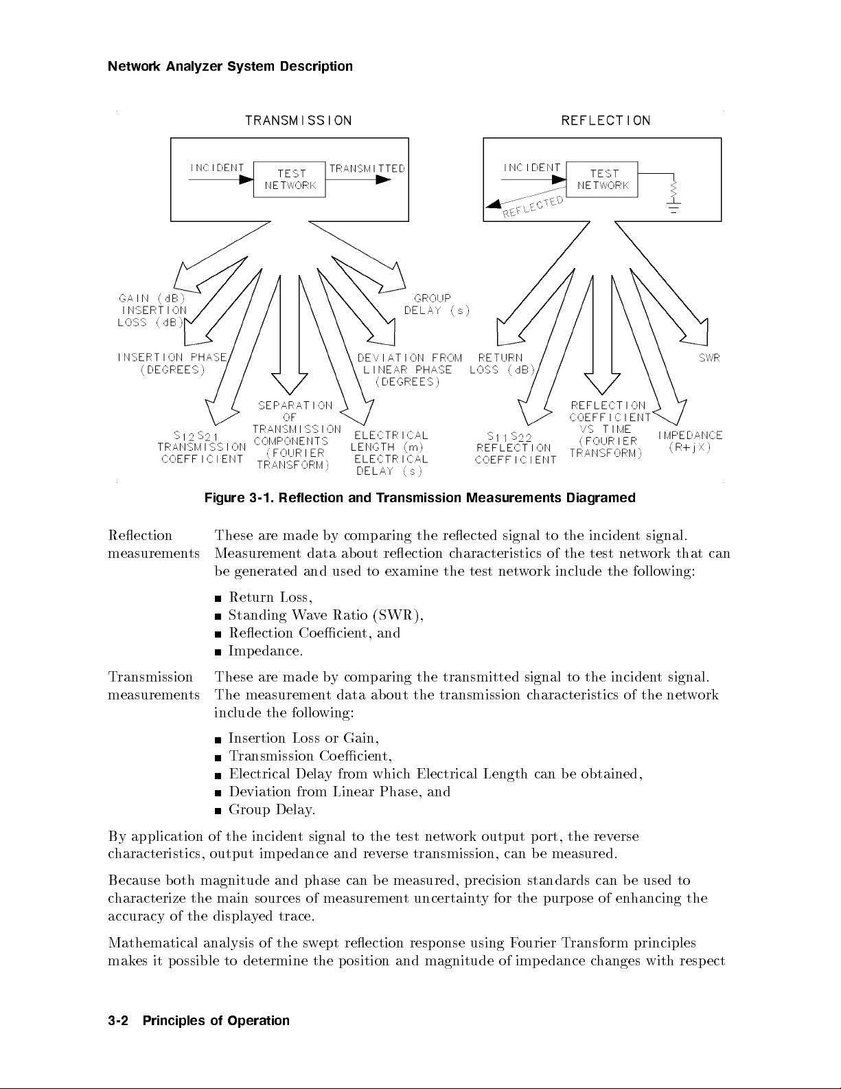
Network Analyzer System Description
Figure 3-1. Reflection and Transmission Measurements Diagramed
Reection
measurements
These are made by comparing the reected signal to the incident signal.
Measurement data ab out reection characteristics of the test network that can
be generated and used to examine the test net
work include the following:
Return Loss,
Standing Wave Ratio (SWR),
Reection Coecient, and
Impedance.
Transmission
measurements
These are made by comparing the transmitted signal to the incident signal.
The measurement data ab out the transmission characteristics of the network
include the following:
Insertion Loss or Gain,
Transmission Co ecient,
Electrical Delay from which Electrical Length can be obtained,
Deviation from Linear Phase, and
Group Delay.
By application of the incident signal to the test network output port, the reverse
characteristics, output impedance and reverse transmission, can be measured.
Because both magnitude and phase can be measured, precision standards can be used to
characterize the main sources of measurement uncertainty for the purpose of enhancing the
accuracy of the displayed trace.
Mathematical analysis of the swept reection response using Fourier Transform principles
makes it possible to determine the position and magnitude of imp edance c
hanges with respect
3-2 Principles of Operation
Page 64

Network Analyzer System Description
to a reference plane. Similarly, analysis of the transmitted resp onse allows you to examine
dierent signal paths.
These measurements and accuracy enhancement techniques are further described in this
chapter.
System Block Diagram
Figure 3-2 is a simplied block diagram of the general-purpose 8510 network analyzer system.
Figure 3-2. Simplified System Block Diagram
Description of the 8510 Network Analyzer
The 8510 is a high performance vector receiver. The instrument has four inputs, two
independent measurementchannels, and an internal microcomputer to automate
measurements, conduct data processing, display results, and manage data input/output
operations.
The dedicated system bus provides fast digital communication between individual system
instruments, allowing the network analyzer to fully use the source and test set capabilities.
The interface also provides direct data transfer to the hardcopy device for p ermanent records
of measurement displays.
Principles of Operation 3-3
Page 65

Network Analyzer System Description
How the 8510 Makes Measurements
In a typical measurement, the signal source is swept from the lower measurement frequency
to the higher measurement frequency using a linear ramp controlled by the 8510. The sweep
is called a ramp sweep. Ramp sweep oers the fastest update of the measurement display.
In step-sweep mo de, the source is phase-locked at each discrete measurement frequency
controlled by the 8510.
At the rst frequency conversion stage, signal separation components in the test set apply
a portion of the incident signal and the resp onses from the device under test to the rst
stage. Digital communication between the receiver and the test set pre-tunes the 65 MHz to
300 MHz voltage-tuned local oscillator (VTO) so that one of its harmonics mixes with the
stimulus to produce a 1stIF frequency close to 20 MHz.
Fine tuning is accomplished by comparing the IF frequency with the internal 20 MHz crystal
reference and sweeping the local oscillator to track the stimulus frequency.
When the local oscillator reaches its upper frequency limit, the sweep is stopped, the lo cal
oscillator is tuned again, phase lock is reestablished, and the sweep is continued. Since the
rst local oscillator frequency is selected algorithmically from a known stimulus frequency, the
measurement is free of harmonic skip.
The second frequency conversion produces an IF frequency of 100 kHz for application to the
detection and data processing elements of the receiver. Because the frequency conversions
are phase-coherent and the IF signal paths are carefully matc
hed, magnitude and phase
relationships between the input signals are maintained throughout the frequency conversion
and detection stages. Automatic, fully calibrated, autoranging IF gain steps main
tain the IF
signal at optimum levels for detection over a wide dynamic range.
Test and Measurement Input Channels
Each measurementchannel can use either input a
or a2as the reference signal; b1and b2are
1
always used for the test signal.
The unused reference channel can be used to measure a third test signal. F
assume you choose a
as the phase-locking reference channel. You can now use a
1
or example,
as a third
2
measurementchannel.
Ratio Measurements and Sampling Details
Depending upon the test set conguration, the appropriate reference input and test input are
ratioed to obtain the measurement.
During a ramp sweep, the selected inputs are sampled up to 801 times, with sample timing
accomplished by sensing the 0 to 10 V sweep output from the source. For example, with 401
points selected, at each positive 0.025 V change in the sweep voltage, all selected inputs are
sampled and applied to the reference and test synchronous detectors.
In step sweep, the selected inputs are sampled a certain interval after phase lockis
established.
Each synchronous detector develops the real (X) and imaginary (Y) values of the reference,
or test signal, by comparing the input with an internally generated 100 kHz sine wave. This
method practically eliminates measurement uncertainty errors resulting from drift, osets,
and circularity. Each X,Y data pair is sequentially converted to digital values and read by the
central processing unit (CPU).
3-4 Principles of Operation
Page 66

Network Analyzer System Description
Digital Signal Processing
Digital signal processing (DSP), Figure 3-3, proceeds under control of the 8510 rmware
operating system executed by the main CPU (central processing unit).
CPU and Memory Description
The CPU is a 32-bit Motorolla 68000 microprocessor equipped with 1 Mbyte of RAM, and
512 Kbytes of EEPROM. The rmware operating system is stored p ermanently in non-volatile
memory, then loaded into active (volatile) memory each time power is applied.
The CPU takes advantage of multi-tasking software architecture, and several distributed
processors, to provide a very fast data-acquisition and display-update rate. The CPU accepts
the digitized real and imaginary data, corrects for IF gain and quadrature errors before the
reference and test pairs are ratioed. If 0 is selected, the data is averaged, then stored in
channel 1 or channel 2 raw data array.
The constants used in this IF correction are obtained periodically with an automatic
self-calibration operation that is invisible to the operator.
Data Processing Steps
While data acquisition software is continually lling the raw data arrays, the data processing
software is processing the data for the t
wo independent displaychannels.
If error correction is turned on, the ra
w data and error coecients from the selected
calibration coecient set are used in appropriate computations by a dedicated vector math
processor.
Next, magnitude and phase osets commanded by the electrical delay, reference plane
extensions, magnitude oset, and magnitude slope under the RESPONSE men
are added to the data. If time-domain mode is a
is converted from the frequency domain to time domain using the in
vailable and selected, the corrected data
verse Fourier Chirp-Z
u structure
transform technique. The results are stored into the corrected data arrays.
Memory arrays are lled from the corrected data arra
y,by control of the user, with trace data
for use in vector computations with current corrected data. If trace math is selected, vector
multiplication, division, addition, or subtraction is performed.
Results are formatted according to the FORMAT selection, point-to-point smoothing is
applied, if selected, and stored into the formatted data arrays. Traces are now scaled, then
sent to the display memory where the trace data is combined with dierent display annotation
data.
A dedicated display pro cessor asynchronously converts the formatted data and annotations for
viewing at a icker-free rate on the vector-writing display.
Principles of Operation 3-5
Page 67

Network Analyzer System Description
Button Push Detection
When the operating system detects a front panel button push, it responds with one of the
following operations:
Executes the command immediately (as when a parameter change is made).
Makes the function just selected become the active function, then waits until input from the
RPG knob, numeric pad, or step keys (as when there is a scale/division change) is entered.
Displays the respective softkey menu.
Note
Certain function selections abort the data processing operation. For example,
MEASUREMENT
beginning of the data acquisition group. These groups are
or
4
USER PRESET
4
RESTART
5
restarts all measurement related functions to the
NNNNNNNNNNNNNNNNNNNNNNNNNNNNNNNNNNNNNNNNNNNN
FACTORY PRESET
5
. These selections initialize the system to a pre-dened state.
In general, changes to the Instrument Sate of the source are executed after the
currentsweep is completed.
Figure 3-3. Digital Signal Processing
Test Signal Sources
The 8510 network analyzer system accepts any of the follo wing signal sources:
An 8360 Series Synthesized Sweeper
An 834x Series Synthesized Sweeper
An 8350x Series Sweep Oscillator with an 835xx Series plug-in
These sources have the correct analog interface signals and are fully 0 with the 8510 digital
system bus. The system bus allows the net
work analyzer to serve as the system controller by
managing the source using standard GPIB protocol.
3-6 Principles of Operation
Page 68

Network Analyzer System Description
Sources in ramp-sweep mode
All of the of sources can operate in ramp sweep mode. In this mode, the network analyzer
directs the source to sweep in a linear ramp over the selected frequency range.
Synthesized sweepers use the \Lock-and-Roll" tuning technique. With this technique, the rst
frequency of the sweep is set with synthesizer accuracy and a linear analog sweep increases to
the stop frequency.
For narrow frequency sweeps (the width depends upon the frequency range), fully locked
synthesizer performance is obtained over the entire sweep. The sweep oscillator uses an
open-loop YIG-tuned source. Refer to the source specications for frequency accuracy and
resolution details.
Sources in step-sweep mode
Synthesized sweepers can also op erate in the step sweep mode. In this mo de, synthesizer-class
frequency accuracy and repeatability is obtained by phaselocking the source at each frequency
step over the selected frequency range. This mode provides the highest accuracy, although at
reduced measurement sp eed.
Test Sets
Agilent produces many dierent test sets. The conguration needed depends on the frequency
range and measurement capabilities desired. The two most commonly used test set types are
the Reection/Transmission test set and the S-parameter test set. Eac
h test set provides the
following:
Input and output ports for connecting the device to test
Signal separation for sampling the reference signal and test signals
Test signal frequency to 20 MHz conversion
Coaxial Test Set Information
The following information applies to coaxial test sets for measuremen
sets for other frequency ranges are described in their appropriate documen
ts up to 26.5 GHz. Test
tation.
With standard coaxial test sets, the frequency converter is fully integrated into the signal
separation path, and provides optimum performance. Parameter selection is controlled from
the network analyzer front panel.
Principles of Operation 3-7
Page 69

Network Analyzer System Description
Reflection/Transmission Test Sets
Several models of the reection/transmission test set are available. See Figure 3-4 for a signal
ow diagram of a typical Reection/Transmission test set. The test sets provide automatic
selection of S11or S21.
If parameter S21or S22is selected, it is assumed that the op erator has manually reversed the
device under test. Fully error-corrected measurements for one-port devices can be made using
the 1-port calibration procedure.
The one-path 2-port calibration procedure provides full error correction for two-port devices if
the DUT is manually reversed. Note that an attenuator is connected at the device end of the
transmission return cable.
Figure 3-4. Reflection/Transmission Test Set Signal Flow
3-8 Principles of Operation
Page 70

Network Analyzer System Description
S-Parameter Test Sets
S-parameter test sets (shown in Figure 3-5) provide automatic selection of S11,S21,S12, and
S22. The stimulus is automatically switched for forward and reverse measurements. This
capability allows for fully error-corrected measurements on one-port devices and two-port
devices without needing to manually reverse the DUT. By taking the ratio after electronic
switching, switching path repeatability errors are eliminated.
The bias input and sense connections provided allow the testing of active devices. Internal
10 dB steps attenuators (from 0 dB to 90 dB), are available to control the incident stimulus
level at the DUT input, without causing a change in the reference signal level.
Figure 3-5. S-Parameter Test Set Signal Flow
Principles of Operation 3-9
Page 71

Network Analyzer System Description
Customized Test Sets
To congure signal separation of your own design, use the 8511A frequency converter (see
Figure 3-6). The converter do es not include signal separation devices, thus allowing you to
construct a test set and connect the reference and test signals to the frequency converter
inputs.
If your test setup do es not follow the standard conventions of the reection/transmission or
S-parameter test set, use the
system to select appropriate reference and test inputs to use.
NNNNNNNNNNNNNNNNNNNNNNNNNNNNNNNNNNNNNNNNNNNNNNNNNNNNNNNN
REDEFINE PARAMETER
function sequence in the network analyzer
Figure 3-6. 8511A Frequency Converter Signal Flow
3-10 Principles of Operation
Page 72

Network Analyzer System Description
Measurement Accessories
Source Output-to-Test-Set Input Signal Cable
Use a high quality source-to-test-set cable set to minimize loss and instability. The preferred
source-to-test set cable set is part number 08513-60009. This set has has a 3.5-mm male
connector on one end and the 3.5-mm female connector on the other. These cables havelow
loss and are rugged.
Test Port Return Cables
High quality cables, attenuators, and adapters to connect between the test set ports and
the device under test are essential to achieve accurate, repeatable measurements. Worn or
unstable cables and connectors increase measurement errors due to directivity, mismatch,
and frequency response eects. Check cables and connectors regularly and replace them as
necessary.
Test p ort return cables used with the network analyzer system must be durable and stable,
and care is required to avoid damaging them. Cables can be destroyed by bending with to o
tight a radius. Because even with careful use, cables wear out eventually, treat all cables as
consumable items to be replaced as often as necessary
. The most importantcharacteristic of
all cables is minimum magnitude and phase change between movements (exures) of the cable.
Replace a cable when unacceptable magnitude and/or phase c
hanges occur when the cable is
moved.
The standard recommended cables, in good condition, m
verication of the analyzer system. These cable sets ha
match, and high return loss, and they are stable in use. F
ust be used for detailed performance
velow insertion loss, go od electrical
or other applications, any high
quality cable set can b e used.
Extension Lines
External signal path extension lines connected to the test set rear panel EXTENSION A and
EXTENSION B connectors are used to balance the reference and test signal path lengths
according to the port 1 and port 2 connections to the test device. Balancing the reference
and test signal path lengths can b e important when making measurements requiring highest
accuracy. Signal path balance is less imp ortant when using the synthesized sweeper in the
step sweep mo de.
The extension lines are provided in two lengths: long, which has several loops, and short.
Figure 3-7 shows the recommended conguration of theses extension lines for the standard
coaxial test sets.
Principles of Operation 3-11
Page 73

Network Analyzer System Description
Figure 3-7. Recommended Typical Test Setups
3-12 Principles of Operation
Page 74

Network Analyzer System Description
For the reection/transmission test sets, when connecting the DUT directly to port 1, use
the short extension lines. On these test sets, the Extension B line is in the test signal path,
making it possible to add bias tees, step or xed attenuators, ampliers, isolators, or other
signal-conditioning devices.
For the S-parameter test sets, when using a standard test setup with the DUT connected at
the ends of the equal length test port extension cables, use the long rear panel extension lines.
When connecting the DUT directly at port 1 and using a single transmission return cable, use
the short extension line on Extension B.
You may observe the relative signal path length by observing the uncorrected phase response
of the short circuit and the thru connections. If non-standard test port extension cables are
used, the Extension Lines maybe changed to other lengths of high quality cable (low insertion
loss, high return loss, stable in use) in order to balance electrical lengths.
Adapters (To Protect Test Ports from Wear)
To preserve the port connectors on the test set, avoid connecting any device under test
directly to the test set ports. Always use a high quality adapter or cable as a \connector
saver" to avoid damage and wear to the cable connector. Use only high-quality adapters such
as those supplied in the Agilent calibration kits. Connect an appropriate cable to the test set
port, then connect an adapter that mates to the device under test to the end of this cable.
Proper Connector Care and Use
Keep all connector mating surfaces clean, insp ect all connectors visually before ev
use connector gages to verify that the mating tolerances are within specications. Alw
ery use, and
ays
use a calibrated torque wrench, set to the correct torque, when tightening or removing
connections.
Calibration Kits
Use only the highest quality calibration standards: devices that ha
ve a known response and
are stable in use. Only calibration devices that have an accuracy equal to or greater than
those in HP calibration kits can provide the calibration and error correction accuracy needed
to achieve full, specied measurement accuracy with the 8510 network analyzer system.
Also be aware that calibration standards, like all devices, can become worn and unstable
with use. When a calibration device is no longer stable and repeatable, or if it shows signs of
connector damage or wear, replace it. Detailed handling and storage instructions appear in
the calibration kit operating and service man
uals.
Atypical calibration kit contains a shielded open circuit, a short circuit, xed and sliding
loads, a connector gage, gage calibration blo cks and aligning pins, extra precision 6-slot
center collets, a center collet extractor, a connector torque wrench, and a calibration kit
denition data cartridge. The calibration kit denition data cartridge contains the nominal
characteristics for each of the calibration devices in the kit.
If you use other than a standard Agilent calibration kit, you can dene the standard's nominal
characteristics from the analyzer front panel using the
\Modifying A Calibration Set," at then end of Chapter 8. After y
NNNNNNNNNNNNNNNNNNNNNNNNNNNNNNNNNNNNNNNNNNNN
MODIFY CAL SET
ou dene the calibration kit
feature explained
standards, you can store the data on disc and reload the data as required.
Principles of Operation 3-13
Page 75

Network Analyzer System Description
Verification Kits
Performance verication standards are used to determine that the system can be calibrated
and can produce goo d measurement results. Devices in the verication kits are precision
devices that should not be used on a day-to-day basis. These devices have been characterized
on a standards-class network analyzer by exp erienced Agilent p ersonnel. If you use prop er
calibration and measurement techniques, your measurement results should be comparable
to the data supplied with the devices, within the system sp ecications. The typical
Agilentverication kit includes xed attenuators, a b eadless air line, and a beadless,
stepped-impedance, two-port air line mismatch standard. Data for the devices includes a
device data sheet that lists traceable fully error-corrected data and measurement uncertainty
data on all devices in the kit at various specied frequencies. This measurement uncertainty
includes both the uncertainty of the Agilent measurement system and the sp ecied
uncertainty of the recommended test system.
For detailed system performance verication instructions, refer to Chapter 8, \Specications
and Performance Verication," in the
For information concerning the use and care of the test set, test cables, adapters, calibration
kits, and verication kits, refer to their respective manuals. These are supplied with your
system.
Agilent 8510C On-Site Service Manual.
3-14 Principles of Operation
Page 76

Automatic Recall of Instrument Settings
Automatic Recall of Instrument Settings
The receiver remembers most measurement settings when you switch back and forth between
channels, domains, parameters, or display formats. (This feature remembers all measurement
settings
except
stimulus settings.) This feature is automatic, and does not require you to use
the Save or Recall functions. The feature is called \limited instrument state memory."
Limited instrument state memory works by assigning a hierarchy to the instrument settings.
The hierarchy is as follows:
Channel (1 or 2)
Domain (Frequency, Time, or Power)
Parameter (1, 2, 3, or 4)
Format (any display format)
Response (scale and reference line)
Every mode in the above list
remembers
all settings you make that are
lower in the hierarchy
For example, assume you choose the following measurement settings.
Channel 1
Power Domain
Parameter 3
Log mag (format)
Reference010 dB
Scale 5 dB/div
Nowyou go to Channel 2 and make completely dierent settings.
When you go back to Channel 1, the settings shown above automatically resume. This
hierarchical memory applies to all the controls in the above list.
The Added Benefit of the SAVE/RECALL Feature
Stimulus settings are not part of the limited instrumen
t state memory explained above. To
save stimulus settings along with all the other settings, you must use the SAVE/RECALL
feature. Two other advantages of the Save/Recall feature are:
Saved instrument states can be stored to disc.
Instrument states saved to Save/Recall register 8 becomes the default po
wer-ON or User
Preset state.
.
Principles of Operation 3-15
Page 77

Factory Preset State
Factory Preset State
The Factory Preset State consists of the factory default values selected for various functions.
The following table lists the preset state or value associated with a function. If you havea
question about a specic function, refer to its individual entry in the
Dictionary
.
Agilent 8510C Keyword
Table 3-1. Factory Preset Conditions for the 8510C
CAL
DOMAIN
DISPLAY
MARKER
STIMULUS
PARAMETER
FORMAT
RESPONSE
CORRECTION OFF,
Z0= 50, PORT EXTENSIONS 1 and 2 = 0 seconds,
VELOCITY FACTOR = 1.0,
TRIM SWEEP = 0,
CAL SETS 1-8 = Not Changed
FREQUENCY DOMAIN
GATE OFF
SINGLE CHANNEL, DATA
Trace Memories 1-8 Not Changed
Display Colors Not Changed
Date/Time ClockOn
all OFF,4OFF,
DISCRETE
Marker List On, 1 Marker per Parameter
Maximum sweep range of source and test set
NUMBER OF POINTS = 201,
Source Power = depends up on the source
Test Set Attenuation = 0 dB,
SWEEP TIME = 166 ms, RAMP SWEEP, CONTINUAL,
COUPLED CHANNELS
Channel 1 = S
, Channel 2 = S
11
21
Channel 1 = LOG MAG. Channel 2 = LOG MAG
SCALE = 10 dB/division,
REF VALUE = 0 dB, REF POSN = 5,
ELECTRICAL DELAY = 0 seconds, COAXIAL,
AVERAGING = OFF, SMOOTHING = OFF,
PHASE OFFSET = 0 degrees, MAGNITUDE OFFSET = 0 dB,
MAGNITUDE SLOPE = 0 dB/GHz
INSTRUMENT
STATE
COPY
SYSTEM
3-16 Principles of Operation
Selected Channel = 1, No Menu Displayed
SAVE/RECALL Instrument States 1-8 Not Changed.
PLOT ALL = FULL PAGE
S11Data = Pen 3
S21=Pen 5
Plot Type = Color
GPIB Addresses Not Changed
LCD/CRT ON, IF GAIN = AUTO
MULTIPLE SOURCE = OFF
Page 78

Factory Preset State
Hardware State
In general, the Hardware State functions are those that are required for proper operation at
power up and relate more to the hardware conguration of the analyzer. These functions are
not aected by pressing either
4
USER PRESET
NNNNNNNNNNNNNNNNNNNNNNNNNNNNNNNNNNNNNNNNNNNN
5
or
FACTORY PRESET
.Values or text shown in
parenthesis are factory default settings.
Table 3-2.
Hardware State Setting
GPIB Addresses
FFFFFFFFFFFFFFFFFFFFFFFFFFFFFFFFFFF
ADDRESS of 8510
FFFFFFFFFFFFFFFFFFFFFFFFFFFFFFFFFFFFFFFFFFFFFFFF
ADDRESS of SYSTEM BUS
F
FFFFFFFFFFFFFFFFFFFFFFFFFFFFFFFFFFFFFFFFFFFFF
ADDRESS of SOURCE #1
FFFFFFFFFFFFFFFFFFFFFFFFFFFFFFFFFFFFFFFFFFFF
ADDRESS of TEST SET
F
FFFFFFFFFFFFFFFFFFFFFFFFFFFFFFFFFFFFFFFF
ADDRESS of PLOTTER
FFFFFFFFFFFFFFFFFFFFFFFFFFFFFFFFFFFFFFFFF
ADDRESS of PRINTER
F
FFFFFFFFFFFFFFFFFFFFFFFFFFFFFFFFFF
ADDRESS of DISC
F
FFFFFFFFFFFFFFFFFFFFFFFFFFFFFFFFFFFFFFFFFFFFF
ADDRESS of SOURCE #2
F
FFFFFFFFFFFFFFFFFFFFFFFFFFFFFFFFFFFFFFFFFFFFF
ADDRESS of PASS-THRU
F
FFFFFFFFFFFFFFFFFFFFFFFFFFFFFFFFFFFFFFFFFFFFF
ADDRESS of RF SWITCH
F
FFFFFFFFFFFFFFFFFFFFFFFFFFFFFFFFFFFFFFFFFFFFFFF
ADDRESS of POWERMETER
(16)
(GPIB, 5)
(GPIB, 1)
(0)
(17)
(19)
(20)
(31)
(31)
(31)
(13)
Disc Unit Number (0)
Disk Volume Number (0)
System Phaselo ckType (Internal)
System Phaselo ck Sp eed (Normal)
System Phaselo ck Step Type (Reads Source in System to Determine)
Multiple Source Values RF Source #1
Numerator (1)
Denominator (1)
Oset (0)
LO Source #2
Numerator (0)
Denominator (1)
Oset (0)
Receiver
Numerator (1)
Denominator (1)
Oset (0)
GPIB Resp onse to
PRES;
Command (User Preset)
Warning Beep er (On)
Power Level RF Source #1 (0 dBm)
Power Level LO Source #2 (0 dBm)
Principles of Operation 3-17
Page 79

Factory Preset State
Table 3-2. (continued)
Hardware State Setting
LCD/CRT Display Colors Background Intensity (0%)
External Video Synchronization (Sync on Green, Negative)
Power Leveling Source 1 (internal)
Softkeys (Bright White)
Warnings (Bright Red)
S11Data (Bright Yellow)
S22Data (Bright Green)
S21Data (Bright Cyan)
S12Data (Bright Salmon)
Graticule (Dim Grey)
Marker Symbols (White)
S11Memory (Medium Yellow)
S22Memory (Medium Green)
S21Memory (Medium Cyan)
S12Memory (Medium Salmon)
Stimulus Values (Medium White)
Source 2 (internal)
3-18 Principles of Operation
Page 80

Measurement Controls
Measurement controls include the following menu blocks and front-panel keys, which are
described in this chapter in the following alphabetical order:
Display
Domain
Marker
Parameter
Response
Stimulus
Display
4
Press the
Note
4
DISPLAY
5
key in the MENUS blo ck to bring the Display menuonto the CRT/LCD.
The original 85101 (top box) of 8510 systems incorporated a cathode ra
(CRT) based display. The current design incorporates a liquid crystal display
(LCD). Display references apply to b oth designs unless noted otherwise.
Choices under the Display menu allow you to choose:
Single channel, single parameter, or
Single channel, four parameter, or
Dual channel displays.
The color attributes of the CRT/LCD.
External video interface selections (CRT only).
Limit lines and limit point measurements.
Storage (to memory) and display of complete traces.
Complex trace math using the current data and a trace stored in memory or the current
data from either channel.
y tube
Measurement Controls 4-1
Page 81

DISPLAY Functions
Display Modes
The display mode menu is shown in Figure 4-1.
Figure 4-1. Display and Display Mode Menus
Figure 4-2 shows one p ossible LCD/CRT display and its annotation areas. Figure 4-3 shows
the annotation areas for the four parameter split displa
y mode.
Figure 4-2. Annotation Areas for Single Parameter or Dual Channel Display Mode
4-2 Measurement Controls
Page 82

DISPLAY Functions
Figure 4-3. Annotation Areas for Four Parameter Split Display Mode
The annotation areas are explained in Chapter 1, \Principles of Operation." Note that the
following annotation areas stay in the same location regardless of the displa
ActiveEntry System Messages
Enhancement Annotation Stimulus Values
Softkey Menu Display Measurement Display
NNNNNNNNNNNNNNNNNNNNNNNNNNNNNNNNNNNNNNNNNNNNNNNNNN
SINGLE PARAMETER
Dual Channel Display Modes
In dual channel op eration, the currentchannel 1 and channel 2 measurements are displayed at
the same time.
NNNNNNNNNNNNNNNNNNNNNNNNNNNNNNNNNNNNNNNNNNNNNNNNNNNNN
DUAL CHAN OVERLAY
channel. A dual channel overlay trace showing Log Mag for both channels is shown in
Figure 4-4, although any parameter, format, and response settings can b e selected for either
channel. For Cartesian displays, trace labels identify the traces for the twochannels: the
label1(identifying the trace from channel1)appears on the left of the graticule; the label
(channel2)appears on the right of the graticule.
NNNNNNNNNNNNNNNNNNNNNNNNNNNNNNNNNNNNNNNNNNNNNNN
DUAL CHAN SPLIT
Channel 1 measurements are on the left, channel 2 measurements on the right.
is the Factory Preset state, with channel 1 displaying S
displays both measurements full size on the format selected for each
displays the measurements on two half-size graticules side by side.
y mode.
.
11
2
Measurement Controls 4-3
Page 83

DISPLAY Functions
Figure 4-4. Dual Channel Overlay and Split Displays
Operation in dual channel is the same as for single channel. Tochange the measurement
setup, rst select the channel, press
The Parameter, Format, and Response functions are selected independen
If you wanttocho ose dierent Stimulus functions for eachchannel, you must rst \uncouple"
the channels by pressing STIMULUS
4
CHANNEL 1
4
5
MENU
5or4
NNNNNNNNNNNNNN
MORE
5
CHANNEL 2
, then make the control settings.
NNNNNNNNNNNNNNNNNNNNNNNNNNNNNNNNNNNNNNNNNNNNNNNNNNNNNNNN
UNCOUPLED CHANNELS
tly for eachchannel.
(see Stimulus for
details).
To return to a single-channel display, press
4
DISPLAY
NNNNNNNNNNNNNNNNNNNNNNNNNNNNNNNNNNNNNN
5
,
DISPLAY MODE
NNNNNNNNNNNNNNNNNNNNNNNNNNNNNNNNNNNNNNNNNNNNNNNNNN
SINGLE PARAMETER
.
4-4 Measurement Controls
Page 84

DISPLAY Functions
Single Channel, Four Parameter Display Modes
Four parameter display mo des are useful for viewing all four S-parameters or a combination of
S-parameters with User parameters at the same time.
NNNNNNNNNNNNNNNNNNNNNNNNNNNNNNNNNNNNNNNNNNNNNNNNNNNNNNNN
FOUR PARAM OVERLAY
displays all four parameters full size in the format selected for each
parameter. In four parameter overlay display mo de, information for all four parameters
appears at the top of the display in the following format:
S
11
DISPLAY FORMAT S
12
REFERENCE LINE VALUE SCALE REFERENCE LINE VALUE SCALE
S
21
DISPLAY FORMAT S
22
REFERENCE LINE VALUE SCALE REFERENCE LINE VALUE SCALE
User parameters are shown in the following locations:
USER 1 DISPLAY FORMAT USER 3 DISPLAY FORMAT
REFERENCE LINE VALUE SCALE REFERENCE LINE VALUE SCALE
USER 2 DISPLAY FORMAT USER 4 DISPLAY FORMAT
REFERENCE LINE VALUE SCALE REFERENCE LINE VALUE SCALE
NNNNNNNNNNNNNNNNNNNNNNNNNNNNNNNNNNNNNNNNNNNNNNNNN
N
FOUR PARAM SPLIT
displays all four parameters in four quarter-sized graticules. In the four
parameter split display mo de (Figure 4-3), parameter iden
directly above the respective trace display.
Adjust Display Menu
DISPLAY FORMAT
DISPLAY FORMAT
tication information appears
In this menu, you can modify the visual characteristics of the display, including its intensity,
and colors.
Note
The original 85101 (top box) of 8510 systems incorporated a cathode ray tub e
(CRT) based display. The current design incorporates a liquid crystal display
(LCD). Display references apply to b oth designs unless noted otherwise.
Intensity
Tochange the overall displayintensity press,
NNNNNNNNNNNNNNNNNNNNNNNNNNNNN
INTENSITY
entries with the
. Use the RPG knob or entry keys to enter the intensityvalue desired. Terminate
4
5
key.
x1
4
DISPLAY
NNNNNNNNNNNNNN
5
NNNNNNNNNNNNNNNNNNNNNNNNNNNNNNNNNNNNNNNNNNNN
MORE
ADJUST DISPLAY
and
For a CRT display, the factory default setting is set to 83%. This setting maximizes display
life.
For an LCD, the factory default setting is set to 100%. It can be adjusted from 100% to
50%.
Measurement Controls 4-5
Page 85

DISPLAY Functions
The intensity level cannot be saved/recalled. It remains as set or returns to the factory
default.
Background Intensity (CRT only)
Background intensity can be changed to anyvalue from 0 to 100%. The factory set value
is zero, to oer the greatest contrast with the intensity level. Background intensity can b e
saved/recalled.
Modify colors
The displayed colors can be changed to any of sixteen dierent colors, saved, and recalled. See
Figure 4-5 for the adjust display menu.
4-6 Measurement Controls
Page 86

DISPLAY Functions
Figure 4-5. Adjust Display Menu
The following sequence of steps demonstrates howtochange, save, and recall the colors for the
displayed elements.
1.
Press
4
DISPLAY
one of the modify colors menu.
2.
Choose one of the various display elements shown on the menu. For example, press
NNNNNNNNNNNNNNNNNNNNNNNNNN
STIMULUS
assigned to the stimulus value notation shown on the display.Nowyou can adjust the
tint, brightness, and color saturation for that color. The tin
settings vary with the display element/color selected.
NNNNNNNNNNNNNNNNNNNNNNNNNNNNNNNNNNNNNNNNNNNN
5
ADJUST DISPLAY
. By selecting the stimulus element, you have actually chosen to mo dify the color
NNNNNNNNNNNNNNNNNNNNNNNNNNNNNNNNNNNNNNNNN
MODIFY COLORS
. This keystroke sequence displays page
NNNNNNNNNNNNNN
MORE
t, brightness, and color default
Measurement Controls 4-7
Page 87

DISPLAY Functions
Press
NNNNNNNNNNNNNNNNNNNNNNNNNNNNNNNN
BRIGHTNESS
. Use the knob to vary the intensity of the color from very dim
a.
(cannot be seen at 0%) to very bright (100%).
Press
NNNNNNNNNNNNNNNNN
COLOR
. Use the knob to vary the color saturation of the the color from white
b.
(0%) to all color (100%).
Press
NNNNNNNNNNNNNN
TINT
. Tint is the continuum of hues on the color wheel, ranging from red,
c.
through green and blue, and back to red.
The tint setting for the primary colors is as follows:
yellow=14
blue (cyan) = 53
red = 0
NNNNNNNNNNNNNNNNNNNNNNNNNNNNNNNNNNN
3. The
RESET COLOR
softkey returns the display element/color to the default color denition
for that color.
NNNNNNNNNNNNNNNNNNNNNNNNNNNNNNNNNNNNNNNNNNNNNNNNNNNNN
4. Press
PREDEFINED COLORS
to display the menu of colors with predened denitions for
tint, brightness, and color.
5.
Choose one of the predened colors, for example
NNNNNNNNNNNNNNNNN
GREEN
. The display element/color turns
green and the last active function, tintvalue in this case, is shown.
6. Tosave the color modications you have made, press
necessary to return to the adjust display menu or press
NNNNNNNNNNNNNNNNNNNNNNNNNNNNNNNNNNN
press
SAVE COLORS
7.
To recall a previously saved color scheme, press
.
4
PRIOR MENU
4
DISPLAY
NNNNNNNNNNNNNNNNNNNNNNNNNNNNNNNNNNNNNNNNN
RECALL COLORS
5
as many times as
NNNNNNNNNNNNNNNNNNNNNNNNNNNNNNNNNNNNNNNNNNNN
5
ADJUST DISPLAY
.
Default Colors
NNNNNNNNNNNNNNNNNNNNNNNNNNNNNNNNNNNNNNNNNNNN
The
DEFAULT COLORS
softkey returns the display attributes to their factory set default colors
and background intensity. The following is a partial list of the default color denitions.
Table 4-1. Default Settings for Display Elements
Display
Element
Color Tint Brightness
%
Color
%
SOFTKEYS white 0 100 0
WARNING red 0 100 100
S11DATA yellow 14 100 100
S22DATA green 38 93 100
S21DATA cyan (blue) 53 100 60
S12DATA salmon 0 100 36
GRATICULE grey 0 49 0
MARKERS white 0 80 0
S11MEM mustard (yellow) 11 70 85
S22MEM green 41 63 85
S21MEM lt. cyan (blue) 60 70 60
S12MEM lt. red 0 75 55
STIMULUS white 0 90 0
.Now
4-8 Measurement Controls
Page 88

DISPLAY Functions
External Video (CRT only)
The network analyzer is designed to work with external video monitors. Use the controls in
the following menu to congure the system for compatibility with a variety of monitors. To
evaluate a display for analyzer compatibility, lo ok for a horizontal scan range that includes
25.5 kHz. None of these controls aect the internal CRT.
Figure 4-6. External Video Menu
The external video connections are made available through the D1191A external video cable,
provided with your analyzer system. Connect the cable to the rear-panel EXTERNAL
DISPLAYmulti-pin connector. Refer to Table 4-2.
To use the analyzer with an HP 35741 or 35742 external monitor, matc
h and connect the red,
green, blue BNC cables and then check the analyzer external video settings for sync-on-green
mode. This synchronization method superimposes the combined horizontal and vertical sync
signals onto the green (analog) video signal. This is done in a manner similar to EIA standard
RS-330 (positive video, negative sync). This is the factory default setting, but once modied,
the new settings are retained in EEPROM and are not modied by
NNNNNNNNNNNNNNNNNNNNNNNNNNNNNNNNNNNNNNNNNNNN
FACTORY PRESET
or by
recalling an Instrument State.
NNNNNNNNNNNNNNNNNNNNNNNNNNNNNNNNNNNNNNNNNNNN
Use
COMPOSITE SYNC
To some external display devices, the polarity of the sync
when the external display device requires a TTL-level composite sync.
hronization signal is signicant. The
composite signal may be either positive or negative logic.
Use horizontal, vertical sync when an external display device requires separate TTL-
compatible synchronization signals. After selecting
NNNNNNNNNNNNNNNNNNNNNNNNNN
H,V SYNC
,check and set, if necessary, the
polarity of the synchronization signal.
NNNNNNNNNNNNNNNNNNNNNNNNNNNNNNNNNNNNNNNNN
Use
NEGATIVE SYNC
when an external display device requires negative logic, TTL-compatible
synchronization.
NNNNNNNNNNNNNNNNNNNNNNNNNNNNNNNNNNNNNNNNN
Use
POSITIVE SYNC
when an external display device requires p ositive logic, TTL-compatible
synchronization.
Measurement Controls 4-9
Page 89

DISPLAY Functions
Table 4-2. External Display Cable Connections
Mode BNC Cable Signal
Red Green Blue Sync
FFFFFFFFFFFFFFFFFFFFFFFFFFFFFF
SYNC ON GREEN
FFFFFFFFFFFFFFFFFFFFFFFFFFFFFFFFF
COMPOSITE SYNC
F
FFFFFFFFFFFFFFFFFFFF
H, V SYNC
External Video (LCD only)
Network analyzers with a liquid crystal display (LCD) installed are designed to work with
external VGA video monitors. The external video connections are made available through the
rear-panel VGA multi-pin connector.
RGB on green/white BNC
RGB on black/white BNC
RGB horizontal (H) on black/white BNC
vertical (V) on brown/white BNC
4-10 Measurement Controls
Page 90

DISPLAY Functions
Limits: Limit Lines and Limit Points Measurements
On the 8510C network analyzer, you can dene limits that are displayed on the screen, while
the trace is displayed. These limits allow you to visually compare the trace values with the
limits that are dened.
In addition to the limits display on the screen, you can select to have the 8510C perform a
numeric
the current trace meets the user-dened limits.
limits, or
PASS/FAIL
FAIL
appears if the trace exceeds the dened limits.
comparison with the dened limits. The comparison will indicate whether
PASS
appears if the trace meets the dened
Types of Limits
There are two limit types:
Limit Lines
This type of limit consists of two end p oints with a line drawn
between the end points. The end points of the line are dened by
a stimulus value, usually a frequency, and a limit value. The limit
line drawn between the two end p oints may be either at or sloping,
depending upon the end point settings. Make certain that you enter
tvalue.
^
Limit Points
an end-pointvalue that is greater than the begin-poin
This type of limit consists of a single p oin
t, having a single stimulus
value and limit value. A limit point is drawn on the displayas
symbol. The sharp point in the^indicates the position of the limit
point.
Limit Testing
For the purpose of limit
either \upper" (maximum) limits, or \low
PASS/FAIL
testing, limit lines and points may be dened as being
er" (minimum) limits. When limit
PASS/FAIL
testing is turned on, the measurement points that are on-screen, and fall within any dened
limits, are tested. Either a
PASSorFAIL
message is displayed relating to the results of the
test.
For limit lines, keep in mind that only data points that are
actually measured
are tested
against the limits. For example, a limit line could end between two measurement points. If
this happens, the end point of the limit line is
not
tested.
Note
For limit lines, only the measurement points that fall between the limit line
end points are tested.
For limit points, if the limit p oint does not fall exactly on a measurement point, then the
nearest actual measurement p oint is used for the limit
PASS/FAIL
test. In addition, any limit
point that is not in the measurement range (o the edge of the display), of course, is not
tested.
When no limits are dened, turning limit testing ON displays a
that are dened, but are not in the curren
t measurement range (they are o the edge of the
PASS
message. Any limits
display), are also not tested.
If desired, limit
PASS/FAIL
may b e turned on without limits being displa
yed.
Measurement Controls 4-11
Page 91

DISPLAY Functions
Limit Tables
Each limit table can consist of from 0 to 12 limits, in any combination of limit lines and limit
points.
An instrument state in the 8510C can contain eight limit tables. There are four tables for
eachchannel, and one table for each of the four \primary" parameters (one each for
S21,S12
, and
S22
, but the same limit table is used for
S11
and
User 1
.) By having multiple
S11
,
limit tables, separate tables of limits may be dened for each parameter while in 4-parameter
display mode.
After a limit table has been created for one parameter on one channel, that table maybe
copied to any other parameter on either of the channels, using the
NNNNNNNNNNNNNNNNNNNNNNNNNNNNNNNNNNN
COPY LIMITS
function.
Figure 4-7. Example of a Limit Test using Limit Lines
Creating a Limit Test
Use the following example to set up an example limit test for an RF lter.
Note
This procedure assumes a device response is displa
yed on the network analyzer
screen.
To Set Up the Measurement
1. Connect the RF lter between the network analyzer RF OUT and RF IN ports.
2. Press
4
PRESET
5,4
FREQ
5
, then
4
CENTER
5
.Enter the center frequency of the RF lter being
tested.
For this example, enter 175 MHz for the c
enter frequency.
4-12 Measurement Controls
Page 92

DISPLAY Functions
3. Press
4
SPAN
5
and enter a frequency span that simplies viewing the passband of the RF
lter.
Use a 200 MHz span, as an example.
4.
Press
4
SCALE
5
then
NNNNNNNNNNNNNNNNNNNNNNNNNNNNN
AUTOSCALE
to view the entire measurement trace.
To Set the Limit Test Values
Limits create boundaries between which an active trace must remain for the measurementto
pass. To develop the limits, you select an appropriate softkey and adjust its p osition (value)
with the RPG, the step keys, or byentering the numeric value via the key pad.
5.
Press
4
DISPLAY
5
then
NNNNNNNNNNNNNNNNNNNN
LIMITS
. The network analyzer display splits into two sections. One
section displays the limit table and the other shows the selected limits on the display.
Press
NNNNNNNNNNNNNNNNNNNNNNNNNNNNN
ADD LIMIT
to display the Add Limit menu.
6.
To Define the Maximum Limit
In the following example, the resp onse of the lter is measured against three maximum limit
lines. The values are determined from the displayed trace, then limit parameters are entered
for a limit test. The values used for determining the limits are as follows:
Location Frequency of Interest
The low side of the cut-o
125 MHz to 150 MHz
frequency portion
The bandpass portion 155 MHz to 195 MHz
The high-side of the cut-o
200 MHz to 225 MHz
frequency portion
There are twoways to dene the test limits:
1. Use a marker to determine the frequencies of the trace you plan to limit test:
NNNNNNNNNNNNNNNNNNNN
Press
MARKER
.
NNNNNNNNNNNNNNNNNNNNNNNNNN
Use the RPG knob to move the marker along the trace, or use the
= MARKER
enter values directly.
2. Or, use the softkeys and the RPG, step k
visually adjust the limits in real-time, ab out the displa
a.
b.
NNNNNNNNNNNNNNNNNNNNNNNNNNNNNNNNNNNNNN
Press
ADD MAX LINE
NNNNNNNNNNNNNNNNNNNNNNNNNNNNNNNNNNNNNNNNNNNN
Press
BEGIN STIMULUS
to set a limit above the device's response trace.
, then enter 125 MHz. This is the beginning frequency value of
eys, or numeric keys in any combination to
yed measurement trace.
the rst, maximum limit line.
key to
Measurement Controls 4-13
Page 93

DISPLAY Functions
Note
Correct a mistakeby using the following technique:
If your incorrect value is entered and you have not pressed
4
MHz
over the error, then enter the correct value.
NNNNNNNNNNNNNNNNNNNNNNNNNNNNNNNNNNNNNNNNNNNN
If you have pressed
4
5
for the incorrect value, press
MHz
BEGIN STIMULUS
and enter the corrected value.
NNNNNNNNNNNNNNNNNNNNNNNNNNNNNNNNNNNNNN
c. Press
END STIMULUS
.Enter 150 MHz, the ending frequency of the rst maximum limit
line. A limit line is drawn b etween the two frequency values you entered, at a zero (0.0)
unit level.
NNNNNNNNNNNNNNNNNNNNNNNNNNNNNNNNNNN
d. Press
BEGIN LIMIT
and watch the limit segment and measurement trace as you rotate
the RPG knob to adjust the b eginning of the limit segment.
e. Place the beginning of the limit line at025 dB, which is the device's maximum
allowable output power level, for the beginning frequency.
Note
Notice that the power level and frequency value appear in the limit-test table.
You can iterate between setting the beginning and ending of the limit line
position.
NNNNNNNNNNNNNNNNNNNNNNNNNNNNN
f. Press
END LIMIT
, and watch the traces on the displayas you rotate the RPG to adjust
the end of the limit segment.
5
, back space
g. Place the end of the limit line at 0.0 dB, whic
h is the device's maximum allowable
output power level, for the ending frequency.
3.
Press
4
PRIOR MENU
5
, then
NNNNNNNNNNNNNNNNNNNNNNNNNNNNNNNNNNNNNN
ADD MAX LINE
. Repeat the above steps for the frequencies of the
second and third maximum limit lines. For this example:
1)
155 MHz to 195 MHz, and2)200 MHz to 225 MHz
4-14 Measurement Controls
Page 94

DISPLAY Functions
To Define Minimum Limit Lines
If desired, use the RPG, step keys, or numeric keypad to dene minimum limits. Minimum
limits may be at frequencies that are dierent from the maximum limit frequencies. It is
acceptable to enter minimum limits before or after entering maximum limits.
For this example, the frequencies used for maximum and minimum limit lines are slightly
dierent. Refer to the table below:
Location Frequency of Interest
The low side of the cut-o
125 MHz to 150 MHz
frequency portion
The bandpass portion 155 MHz to 195 MHz
The high-side of the cut-o
200 MHz to 225 MHz
frequency portion
NNNNNNNNNNNNNNNNNNNNNNNNNNNNNNNNNNNNNN
1. Press
4
PRIOR MENU
5
, then
ADD MIN LINE
to set up the limit line for the device's lower level
response.
2.
NNNNNNNNNNNNNNNNNNNNNNNNNNNNNNNNNNNNNNNNNNNN
Press
BEGIN STIMULUS
and enter 125 MHz, the b eginning frequency of the rst minim
limit line.
Note
Correct a mistakeby using the following technique:
If your incorrect value is entered and you have not pressed
over the error, then enter the correct value.
If you have pressed
4
5
for the incorrect value, press
MHz
4
5
, back space
MHz
NNNNNNNNNNNNNNNNNNNNNNNNNNNNNNNNNNNNNNNNNNNN
BEGIN STIMULUS
and enter the corrected value.
NNNNNNNNNNNNNNNNNNNNNNNNNNNNNNNNNNNNNN
3. Press
END STIMULUS
.Enter 150 MHz, the ending frequency of the rst minim
um limit
line. A limit line is drawn b etween the two frequency values you entered, at a zero (0.0)
unit level.
NNNNNNNNNNNNNNNNNNNNNNNNNNNNNNNNNNN
4. Press
BEGIN LIMIT
and watch the limit segment and measurement trace as you rotate the
RPG knob to adjust the limit segment.
um
5. Place the beginning of the limit line at050 dB, which is the device's minimum allowable
output power level for the beginning frequency.
Note
Notice that the power level and frequency value appear in the limit-test table.
You can iterate between setting the beginning and ending of the limit line
position.
NNNNNNNNNNNNNNNNNNNNNNNNNNNNN
6. Press
END LIMIT
and rotate the RPG to position the end of the limit line at010 dB, the
device's minimum allowable output power level for the ending frequency.
7.
Press
4
PRIOR MENU
5
, then
NNNNNNNNNNNNNNNNNNNNNNNNNNNNNNNNNNNNNN
ADD MIN LINE
and repeat the steps above for the second and
third minimum limit lines. For this example,
1)
155 MHz to 195 MHz, and2)200 MHz to 225 MHz
Measurement Controls 4-15
Page 95

DISPLAY Functions
Figure 4-8. Limit Test Example Using Limit Lines and Limit Points
Editing Limits in the Limits Table
You may edit any individual frequency, limit, or limit line after you have created it. Become
familiar with the information below about modifying a limit v
1.
Press
4
DISPLAY
5
, then
NNNNNNNNNNNNNNNNNNNN
LIMITS
. The display shows the test device response with limit lines
and the tabular listing of the limits set. The highlighted bo
alue:
x surrounding one segment
indicates the currently selected limit for editing.
2. Press the arrow keys or use the RPG to move the highlighted box to the portion of the test
parameter to edit.
3.
NNNNNNNNNNNNNNNNNNNNNNNNNNNNNNNNNNN
Press
EDIT LIMITS
, then press the keys that corresp ond to the p ortions of the limit y
ou
want to edit (b egin frequency, end frequency, b egin limit, or end limit, as an example.
4. Enter new limit values.
5. Press
6.
4
PRIOR MENU
5
to return to the limits menu.
NNNNNNNNNNNNNNNNNNNNNNNNNNNNNNNNNNNNNNNNN
Press
LIMIT TEST ON
to activate the limit test with the new limits. Test results are
displayed on the screen as
PASSorFAIL
.
4-16 Measurement Controls
Page 96

DISPLAY Functions
Trace Memory Operations
You can store a response in one of the eight trace memory locations, then compare the
data with the current measurement trace, in any format. The Display menu provides
softkeys so you can show the data and memory traces individually, or simultaneously. The
NNNNNNNNNNNNNNNNNNNNNNNNNNNNNNNNNNNNNNNNNNNNNNNNNNNNN
DATA AND MEMORIES
softkey displays the menu to use.
In both single- and dual-channel modes, the display data, memory, and trace math op erations
are always uncoupled. You may select memory operations independently for eachchannel.
Storing Trace Data in Memory
Press the
NNNNNNNNNNNNNNNNNNNNNNNNNNNNNNNNNNNNNNNNN
DISPLAY: DATA
4
DISPLAY
5
key in the MENUS blo ck. The factory preset condition selects
for both Channel 1 and Channel 2. This setting displays the trace from the
current trace data.
NNNNNNNNNNNNNNNNNNNNNNNNNNNNNNNNNNNNNNNNNNNNNNN
To store the active trace in memory, press
DATA
!
MEMORYn
(wherenrepresents the memory
location number, 1 through 8). After a factory preset, eachchannel is assigned a separate
memory. The currentchannel selection for the memory is indicated by the number in the
softkey label,
NNNNNNNNNNNNNNNNNNNNNNNNNNNNNNNNNNNNNNNNNNNNNNNNN
DATA
!
MEMORY n
.
To Display a Stored Trace
NNNNNNNNNNNNNNNNNNNNNNNNNNNNNNNNNNNNNNNNNNNNNNN
To display the stored (memory) trace only, press
DISPLAY: MEMORY
. Notice that when the
memory trace is displayed, the numeric trace indicator for the Cartesian display(a1for
channel 1 or a2for channel 2) disapp ears. In addition, the sweep is stopp ed. The parameter
label located in the channel identication area changes to indicate which memory register is
being displayed.
Settings that can and cannot be changed.
to display the stored trace. The STIMULUS menu
active. The marker can be used to read the po
You may select any format and response setting
4
START
5
and
4
STOP
5
key functions are not
wer and frequency values of the memory trace.
To Display Data and Memory Simultaneously
NNNNNNNNNNNNNNNNNNNNNNNNNNNNNNNNNNNNNNNNNNNNNNNNNNNNN
Press
DATA AND MEMORIES
, then press the
NNNNNNNNNNNNNNNNNNNNNNNNNNNNNNNNNNNNNNNNNNNNNNN
DATA and MEMORY
key. The two traces are
displayed in the same grid. The two traces use the same scale per division, reference line
value, and reference line position that was used for the selected data trace. The parameter
label in the channel identication area changes to name the parameter and the memory that is
displayed.
Notice the current data trace is annotated with either a1or a2at the end of the trace. The
memory trace, however is not annotated. The marker reads only the current data trace.
Settings that can and cannot be changed.
The stored trace must be viewed in the same
domain (frequency, time, voltage, or power) as which the data was stored. Changing the
instrument domain before retrieving the data cannot change the data's domain. The same
number of frequency p oints must also be used. If the domain or number of points is changed
prior to retrieving the data, the current memory operation is automatically turned OFF, and
NNNNNNNNNNNNNNNNNNNNNNNNNNNNNNNNNNNNNNNNN
DISPLAY: DATA
is selected.
Measurement Controls 4-17
Page 97

DISPLAY Functions
Most other display details, however, can be the ones chosen for the currently displayed trace
because of the following methodology:
Data is transferred to memory after error correction is p erformed.
Data is transferred to memory after electrical delay is applied.
Data is transferred to memory after time domain conversion is completed.
Data is transferred to memory prior to trace-math op erations.
Refer to Figure 3-3, \Digital Signal Processing" diagram, for a better look at which operations
are a part of the stored trace data.
To Select the Default Memory
Refer to Figure 4-9. On the far, left-hand side is the Display menu. Press the
NNNNNNNNNNNNNNNNNNNNNNNNNNNNNNNNNNNNNNNNNNNNNNNNNNNNN
DATA AND MEMORIES
key. Use the
NNNNNNNNNNNNNNNNNNNNNNNNNNNNNNNNNNNNNNNNNNNNNNN
SELECT DEFAULTS
key to change the
NNNNNNNNNNNNNNNNNNNNNNNNNNNNNNNNNNNNNNNNNNNNNNNNN
DATA
!
MEMORY 1
to be any one of eight memory lo cations. The number in the softkey reects the default
memory location you choose.
NNNNNNNNNNNNNNNNNNNNNNNNNNNNNNNNNNNNNNNNNNNNNNNNN
If you are using Channel 2, the softkey changes to
DATA
!
MEMORY 2
. Again, any of the
other eight memory locations may be selected. Figure 4-9 illustrates the menus available for
the memory operations.
The default settings after a factory preset are as follo
Data for Channel 1 is saved in memory register 1.
Data for Channel 2 is saved in memory register 2.
ws:
4-18 Measurement Controls
Page 98

DISPLAY Functions
Figure 4-9. Display Menu Showing Trace Memory Locations Menu
Measurement Controls 4-19
Page 99

DISPLAY Functions
Refer to the following steps to select a memory location:
1. Select either
2.
Press
4
DISPLAY
3.
4.
NNNNNNNNNNNNNNNNNNNNNNNNNNNNNNNNNNNNNNNNNNNNNNN
Press
SELECT DEFAULTS
Press the key beside the memory register (
4
CHANNEL 1
5
, then press
5or4
CHANNEL 2
NNNNNNNNNNNNNNNNNNNNNNNNNNNNNNNNNNNNNNNNNNNNNNNNNNNNN
DATA AND MEMORIES
5
.
.
. Notice that the currently selected memory register is underlined.
NNNNN
1
through
NNNNN
7
, then
NNNNNNNNNNNNNN
MORE
NNNNN
for
8
) to underline a
dierent default memory register.
5. To leave the setting unchanged, press
Which memory locations are volatile, which are not.
NNNNNNNNNNNNNNNNNNNNNNNNNNNNNNNNNNNNNNNNNNNNNNNNNNNNNNNNNNN
a
DEFAULT to MEMORY n
(wherenrepresents a number 1 through 8). Memory locations 1,
4
PRIOR MENU
5
.
The Display menu reappears after pressing
2, 3, or 4 are non-volatile memory lo cations. Therefore, the contents are retained after an
instrumentpower cycle.
If memory locations 5, 6, 7, or 8 are displayed, these are volatile registers. The contents of
these registers are purged after an instrumentpower cycle.
What is the operational life of non-volatile memory.
4 use a solid-state memory type that can fail after a number of
are used. The quantity is more than 10,000 operations, ho
In addition, memory locations 1, 2, 3, and
NNNNNNNNNNNNNNNNNNNNNNNNNNNNNNNNNNNNNNNNNNNN
DATA
!
MEMORY
operations
wever. In view of this factor, use
memory registers 5, 6, 7, and 8 rather than 1, 2, 3, and 4 for repetitive memory operations.
Trace Math Operations
The trace math operations provide functionality for complicated mathematical calculations
such as:
Vector addition
Vector subtraction
Vector multiplication
Vector division
You can use these functions on the data trace, using a selected memory
operation, from the opposite channel. Following a factory preset sequence, the default math
operation for both channels is
NNNNNNNNNNNNNNNNNNNNNNNNNN
MATH (/)
. This function provides a display showing the ratio
, or in dual channel
between the current trace and the stored trace. Notice that the parameter label in the channel
identication area changes to show the math operation is being performed. The equivalent
equation for this display is as shown:
curr ent tr ace(DAT A
stored trace(MEMORY
)
)
If the current trace and the stored trace are identical, the complex ration between them is one,
and a Cartesian display of the result would be a at line at 0 dB
, or seconds.
Complex math operations are performed on real and imaginary data, from the corrected
data array for the selected channel. Data is processed by the math function
before
display
formatting and therefore, the results may b e viewed in any format. Refer to the following
steps for an example of changing the default trace-math function:
1. Select either
2.
Press
4
DISPLAY
3.
NNNNNNNNNNNNNNNNNNNNNNNNNNNNNNNNNNNNNNNNNNNNNNN
Press
MATH OPERATIONS
4
CHANNEL 1
5
, then press
5or4
CHANNEL 2
5
.
NNNNNNNNNNNNNNNNNNNNNNNNNNNNNNNNNNNNNNNNNNNNNNNNNNNNN
DATA AND MEMORIES
.
and choose the operation you want to become the default setting.
4-20 Measurement Controls
Page 100

4.
Press
4
PRIOR MENU
5
to retain the original setting.
DISPLAY Functions
Figure 4-10. Trace Math Operations Menu Structure
Measurement Controls 4-21
 Loading...