

Page 1

Specifications
The complete Agilent Technologies 4284A specifications are listed in this data sheet. These specifications are the performance standards or limits
against which the instrument is tested. When
shipped from the factory, the Agilent 4284A meets
the specifications listed here.
Measurement Functions
Measurement parameters
|Z| = Absolute value of impedance
|Y| = Absolute value of admittance
L = Inductance
C = Capacitance
R = Resistance
G = Conductance
D = Dissipation factor
Q = Quality factor
Rs= Equivalent series resistance
Rp= Parallel resistance
X = Reactance
B = Susceptance
q = Phase angle
Combinations of measurement parameters
|Z|, |Y| L, C R G
q (deg), q (rad) D, Q, Rs, Rp, G X B
Mathematical functions
The deviation and the percent of deviation of
measurement values from a programmable
reference value.
Equivalent measurement circuit
Parallel and series
Ranging
Auto and manual (hold/up/down)
Trigger
Internal, external, BUS (GPIB), and manual
Delay time
Programmable delay from the trigger command to
the start of the measurement, 0 to 60.000 s in 1 ms
steps.
Measurement terminals
Four-terminal pair
Test cable length
Standard 0 m and 1 m selectable
With Option 4284A-006 0 m, 1 m, 2 m, and 4 m selectable
Integration time
Short, medium, and long (see Supplemental
Performance Characteristics for the measurement
time)
Averaging
1 to 256, programmable
Agilent 4284A
Precision LCR Meter
Data Sheet
Page 2

Test Signal
Frequency
20 Hz to 1 MHz, 8610 selectable frequencies
Accuracy
±0.01%
Signal modes
Normal (non-constant) – Program selected voltage or
current at the measurement terminals when they
are opened or shorted, respectively.
Constant – Maintains selected voltage or current at
the device under test (DUT) independent of
changes in the device’s impedance.
Signal level
Mode Range Setting accuracy
Voltage Non-constant 5 mV
rms
to 2 V
rms
±(10% + 1 mV
rms
)
Constant
1
10 mV
rms
to 1 V
rms
±(6% + 1 mV
rms
)
Current Non-constant 50 µA
rms
to 20 mA
rms
±(10% + 10 µA
rms
)
Constant
1
100 µA
rms
to 10 mA
rms
±(6 % + 10 µA
rms
)
1. Automatic Level Control Function is set to ON.
Output impedance
100 Ω, ±3%
Test signal level monitor
Mode Range Accuracy
Voltage
1
5 mV
rms
to 2 V
rms
±(3% of reading + 0.5 mV
rms
)
0.01 mV
rms
to 5 mV
rms
±(11% of reading + 0.1 mV
rms
)
Current
2
50 µA
rms
to 20 mA
rms
±(3% of reading + 5 µA
rms
)
0.001 µA
rms
to 50 µA
rms
±(11% of reading) + 1 µA
rms
)
1. Add the impedance measurement accuracy [%] to the voltage level monitor
accuracy when the DUT’s impedance is < 100 Ω.
2. Add the impedance measurement accuracy [%] to the current level monitor
accuracy when the DUT’s impedance is ≥ 100 Ω.
Accuracies apply when test cable length is 0 m or 1 m. The additional error when test
cable length is 2 m or 4 m is given as
fm x L[%]
2
where:
fm = Test frequency [MHz]
L = Test cable length [m]
For example,
DUT’s impedance: 50 Ω
Test signal level: 0.1 V
rms
Measurement accuracy: 0.1%
Cable length: 0 m
Then, voltage level monitor accuracy is
±(3.1% of reading + 0.5 mV
rms
)
Display Range
Parameter Range
|Z|, R, X 0.01 mΩ to 99.9999 MΩ
|Y|, G, B 0.01 nS to 99.9999 S
C 0.01 fF to 9.99999 F
L 0.01 nH to 99.9999 kH
D 0.000001 to 9.99999
Q 0.01 to 99999.9
q –180.000° to 180.000°
∆ –999.999% to 999.999%
2
Page 3

Absolute Accuracy
Absolute accuracy is given as the sum of the
relative accuracy plus the calibration accuracy.
|Z|, |Y|, L, C, R, X, G, and B accuracy
|Z|, |Y|, L, C, R, X, G, and B accuracy is given as
Ae+ A
cal
[%]
where:
Ae= Relative accuracy
A
cal
= Calibration accuracy
L, C, X, and B accuracies apply when Dx(measured
D value) ≤ 0.1. R and G accuracies apply when Q
x
(measured Q value) ≤ 0.1. G accuracy described in
this paragraph applies to the G-B combination only.
D accuracy
D accuracy is given as
De+ q
cal
where:
Deis the relative D accuracy
q
cal
is the calibration accuracy [radian]
Accuracy applies when Dx(measured D value) ≤ 0.1.
Q accuracy
Q accuracy Qeis given as
Q
2
xxDa
Qe= ±
1 Q
xxDa
where:
Qx= Measured Q value
Da= D accuracy
Q accuracy applies when Qxx Da< 1.
q accuracy
q accuracy is given as
q
e
+ q
cal
[deg]
where:
qe= Relative q accuracy [deg]
q
cal
= Calibration accuracy [deg]
G accuracy
When Dx(measured D value) ≤ 0.1
G accuracy is given as
where:
Bx= Measured B value [S]
Cx= Measured C value [F]
Lx= Measured L value [H]
Da= Absolute D accuracy
f = Test frequency [Hz]
G accuracy described in this paragraph applies to
the Cp-G and Lp-G combinations only.
Rpaccuracy
When Dx(measured D value) ≤ 0.1
Rpaccuracy is given as
RpxxD
a
Rp=±
DxD
a
[Ω]
where:
Rpx= Measured Rpvalue [Ω]
Dx= Measured D value
Da= Absolute D accuracy
3
–
+
–
+
Page 4
4
Rsaccuracy
When Dx( measured D value) ≤ 0.1
Rsaccuracy is given as
where:
Xx= Measured X value [Ω]
Cx= Measured C value [F]
Lx= Measured L value [H]
Da= Absolute D accuracy
f = Test frequency [Hz]
Relative Accuracy
Relative accuracy includes stability, temperature
coefficient, linearity, repeatability, and calibration
interpolation error. Relative accuracy is specified
when all of the following conditions are satisfied:
1. Warm-up time: ≥ 30 minutes
2. Test cable length: 0 m, 1 m, 2 m, or 4 m
(Agilent 16048 A/B/D/E)
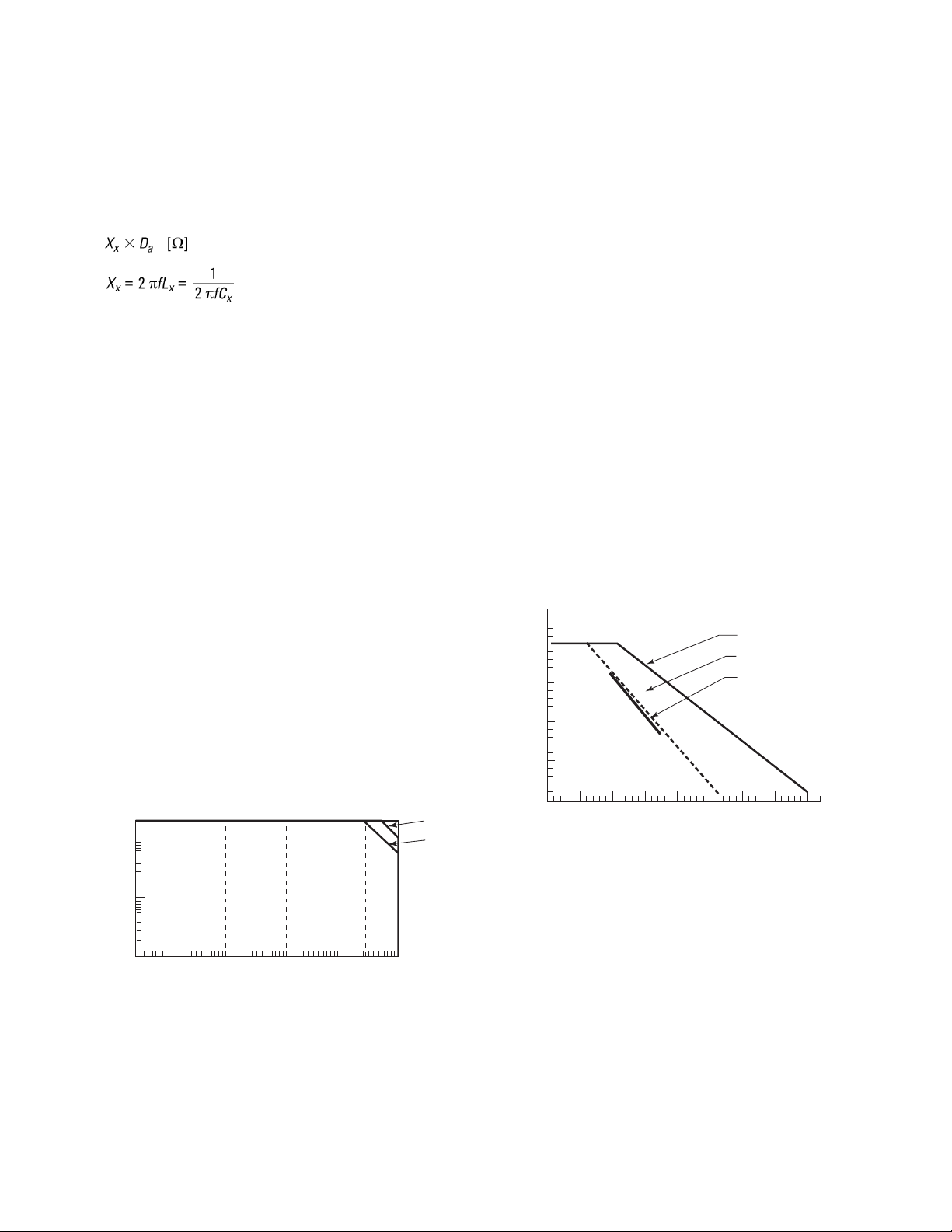
For 2 m or 4 m cable length operation, test signal
voltage and test frequency are set according to
Figure 1-1. (2 m and 4 m cable can only be used
when Option 4284A-006 is installed.)
3. OPEN and SHORT corrections have been
performed.
4. Bias current isolation: Off
(For accuracy with bias current isolation, refer to
supplemental performance characteristics.)
5. Test signal voltage and DC bias voltage are set
according to Figure 1-2.
6. The optimum measurement range is selected
by matching the DUT’s impedance to the effective
measuring range. (For example, if the DUT’s
impedance is 50 kΩ, the optimum range is the
30 kΩ range.)
Range 1: Relative accuracy can apply.
Range 2: The limits applied for relative accuracy
differ according to the DUT’s DC resistance. Three
dotted lines show the upper limits when the DC
resistance is 10 Ω, 100 Ω and 1 kΩ.
Figure 1-1. Test signal voltage and test frequency upper
limits to apply relative accuracy to 2 m and 4 m cable
length operation
20 100 1k
1
1M100k10k
10
20
Test signal voltage (Vrms)
Frequency Hz
2m cable
4m cable
Figure 1-2. Test signal voltage and DC bias voltage upper
limits apply for relative accuracy
Test signal voltage (Vrms)
5302520151004035
DC bias voltage setting (V)
5
0
10
15
20
DC resistance = 1 kΩ
DC resistance = 10 Ω
DC resistance = 100 Ω
Range 1 Range 3Range 2
Page 5

5
|Z|, |Y|, L, C, R, X, G, and B accuracy
|Z|, |Y|, L, C, R, X, G, and B accuracy Aeis given as
Ae= ± [A + (Ka+ Kaa+ KbxKbb+ Kc) x 100 + Kd] xKe[%]
A = Basic accuracy (refer to Figure 1-3 and 1-4)
Ka= Impedance proportional factor (refer to
Table 1-1)
Kaa= Cable length factor (refer to Table 1-2)
Kb= Impedance proportional factor (refer to
Table 1-1)
Kbb= Cable length factor (refer to Table 1-3)
Kc= Calibration interpolation factor (refer to
Table 1-4)
Kd= Cable length factor (refer to Table 1-6)
Ke= Temperature factor (refer to Figure 1-5)
L, C, X, and B accuracies apply when Dx(measured
D value) ≤ 0.1.
R and G accuracies apply when Qx(measured
Q value) ≤ 0.1.
When Dx≥ 0.1, multiply Aeby 1 + D
x
2
for L, C,
X, and B accuracies
When Qx≥ 0.1, multiply Aeby 1 + Q
x
2
for R and
G accuracies.
G accuracy described in this paragraph applies to
the G-B combination only.
D accuracy
D accuracy Deis given as
De= ±
A
e
100
Accuracy applies when Dx(measured D value) ≤ 0.1.
When Dx> 0.1, multiply Deby (1 + Dx).
Q accuracy
Q accuracy is given as
Q
2
xxDe
±
1 QxxD
e
where:
Qx= Measured Q value
De= Relative D accuracy
Accuracy applies when Qxx De< 1.
q accuracy
q accuracy is given as
180 xA
e
π x 100
[deg]
G accuracy
When Dx(measured D value) ≤ 0.1
G accuracy is given as
where:
Bx= Measured B value [S]
Cx= Measured C value [F]
Lx= Measured L value [H]
De= Relative D accuracy
f = Test frequency [Hz]
G accuracy described in this paragraph applies to
the Cp-G and Lp-G combinations only.
–
+
Page 6
6
Rpaccuracy
When Dx(measured D value) ≤ 0.1
Rpaccuracy is given as
RpxxD
e
±
DxD
e
[Ω]
where:
Rpx= Measured Rpvalue [Ω]
Dx= Measured D value
De= Relative D accuracy
Rsaccuracy
When Dx(measured D value) ≤ 0.1
Rsaccuracy is given as
where:
Xx= Measured X value [Ω]
Cx= Measured C value [F]
Lx= Measured L value [H]
De= Relative D accuracy
f = Test frequency [Hz]
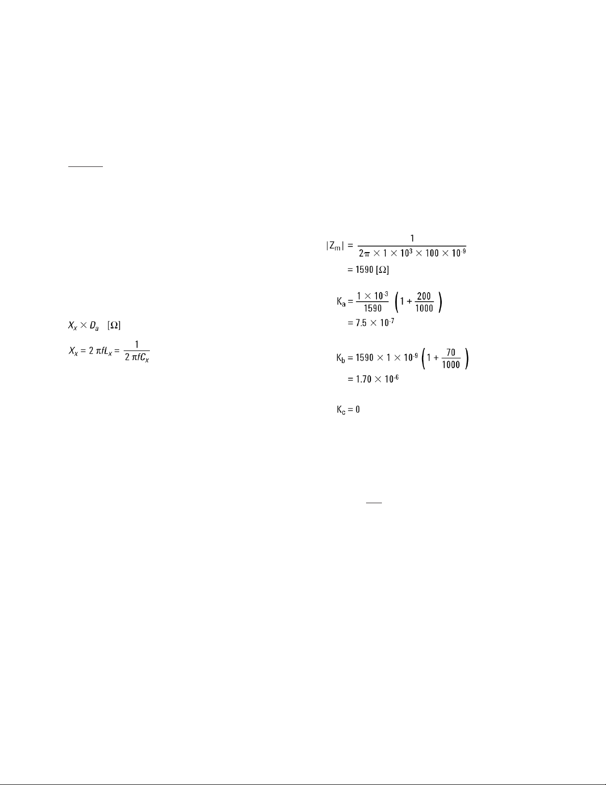
Example of C-D Accuracy Calculation
Measurement conditions
Frequency: 1 kHz
C measured: 100 nF
Test signal voltage: 1 V
rms
Integration time: MEDIUM
Cable length: 0 m
Then:
A = 0.05
Therefore,
C
accuracy
= ±[0.05 + (7.5 x 10⁻⁷+ 1.70 x 10-6) x 100]
≈ ±0.05 [%]
D
accuracy
=±
0.05
100
= ±0.0005
–
+
Page 7
7
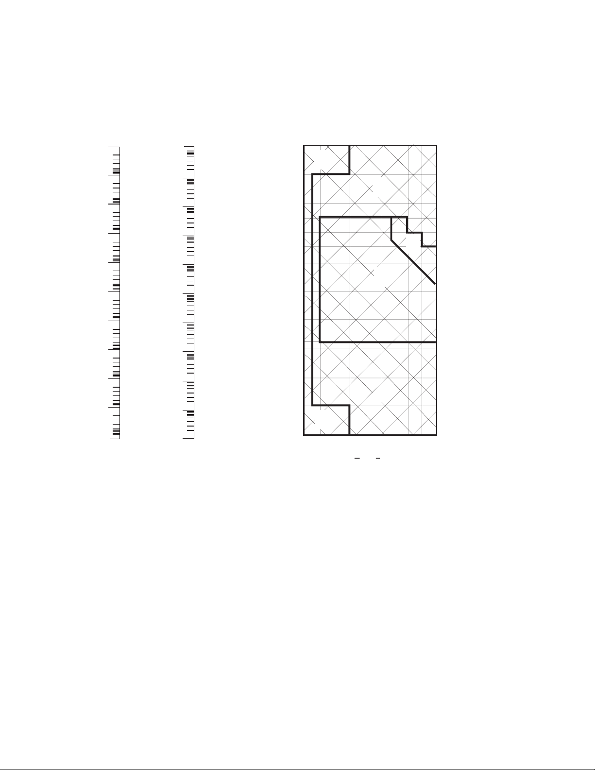
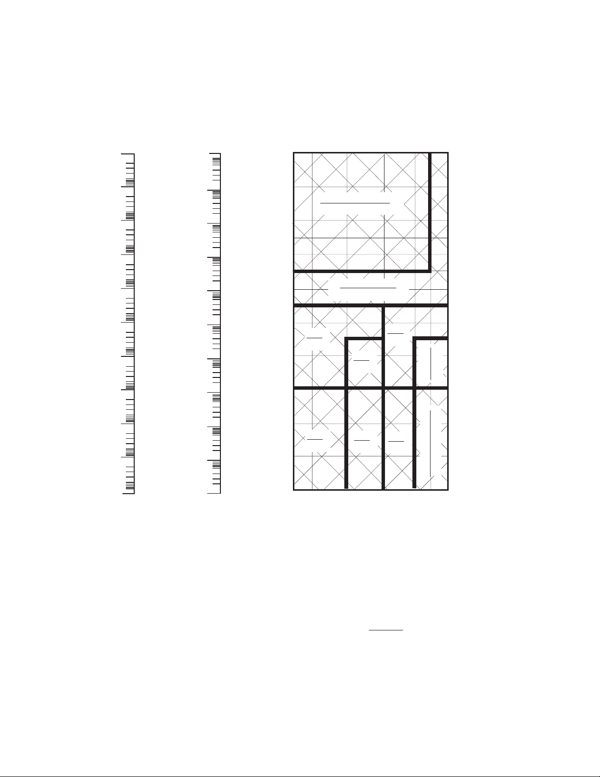
On boundary line apply the better value.
Example of how to find the A value:
0.05 = A value when 0.3 V
rms
≤ Vs≤ 1 V
rms
and
integration time is MEDIUM and LONG.
(0.1) = A value when 0.3 V
rms
≤ Vs≤ 1 V
rms
and
integration time is SHORT.
A1= A value when Vs< 0.3 V
rms
or Vs> 1 V
rms
.
To find the value of A1, A2, A3, and A4refer
to the following table.
where:
Vs= Test signal voltage
100M
10n
100n
1µ
10µ
100µ
1m
10m
100m
1
10
100
100k
32k
10k
320k
1M
10M
1
15
10
100
1k
10m
100m
1
0
0
p
F
1
n
F
1
0
n
F
1
0
0
n
F
1
µ
F
1
0
0
µ
F
1
m
F
1
0
0
m
F
1
0
m
F
20 30 100 1k 10k 100k
30k 300k
1M [Hz]
[S]
|Y| G.B
|Z| R.X
1
0
µ
F
10 H
1 H
100 mH
10 mH
1 mH
100 µH
10 µH
1 µH
100 nH
10 nH
1
0
p
F
1
p
F
1
0
0
f
P
1
0
f
P
100 H
1 kH
10 kH
100 kH
0.1
(0.15)
A4
0.1
(0.2)
A2
0.25
(0.3)
A3
0.05
(0.1)
A1
0.25
(0.3)
A3
0.1
(0.2)
A2
Test Frequency
[Ω]
Specification Charts and Tables
Figure 1-3. Basic accuracy A (1 of 2)
Test frequency
Page 8

8
The following table lists the value of A1, A2, A3, and
A4. When Atl is indicated find the Atl value using
Figure 1-4.
* Multiply the A values as follows, when the test
frequency is less than 300 Hz.
100 Hz ≤ fm<300 Hz: Multiply the A values by 2.
fm< 100 Hz: Multiply the A values by 2.5.
** Add 0.15 to the A values when all of the follow-
ing measurement conditions are satisfied.
Test frequency: 300 kHz < fm≤ 1 MHz
Test signal voltage: 5 V
rms
< Vs≤ 20 V
rms
DUT: Inductor, |Zm| <200 Ω (|Zm|: impedance
of DUT)
A1 = Atl
A
2 = Atl
A
3 = Atl
A
4 = Atl
A
1 = Atl
A
2 = Atl
A
3 = 0.25
A
4 = Atl
A
1 = Atl
A
2 = Atl
A
3 = 0.25
A
4 = Atl
A
1 = Atl
A
2 = 0.1
A
3 = 0.25
A
4 = 0.1
A
1 = Atl
A
2 = Atl
A
3 = 0.25
A
4 = Atl
A
1 = Atl
A
2 = Atl
A
3 = 0.25
A
4 = Atl
A
1 = Atl
A
2 = Atl
A
3 = Atl
A
4 = Atl
A
1 = Atl
A
2 = Atl
A
3 = 0.3
A
4 = Atl
A1 = Atl
A
2 = 0.2
A
3 = 0.3
A
4 = 0.5 X Alt+0.1
A1 = Atl
A
2 = Atl
A
3 = 0.3
A
4 = Atl
A
1 = Atl
A
2 = Atl
A
3 = 0.3
A
4 = Atl
Medium/
long
Short
*
*
**
**
5m 12m 0.1 0.15 0.3 1 2 5 20 [Vrms]
5m 33m 0.15 1 2 5 20 [Vrms]
2.0
1.5
1.0
0.5
0.2
0.1
0.15
0.05
0.02
0.01
5m 10m 20m 50m 100m 200m 500m 1 2 5 10 20 [Vrms]
At1
INTEG TIME
SHORT
MEDIUM
and
LONG
Figure 1-4. Basic accuracy A (2 of 2)
Test signal voltage
Test signal voltage
Page 9
9
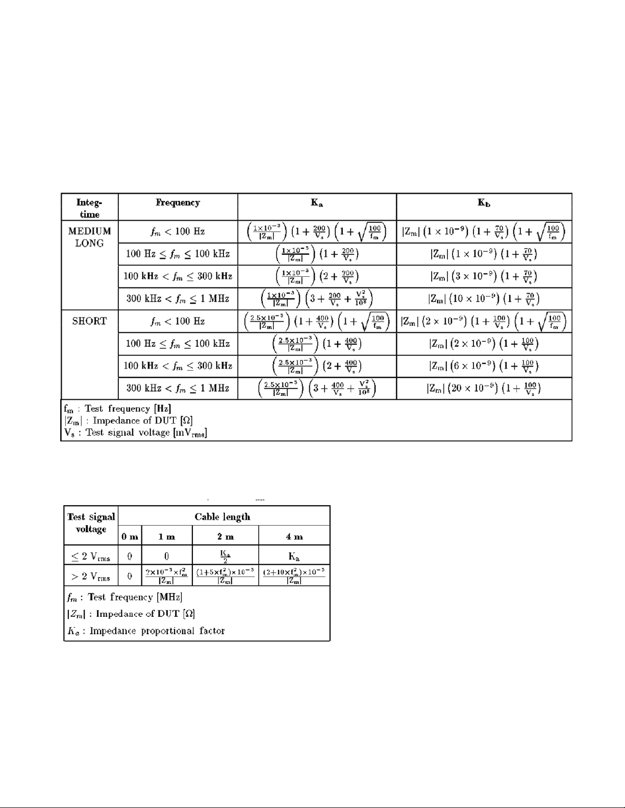
Kaand Kbvalues are the incremental factors in
low impedance and high impedance measurements,
respectively. Kais practically negligible for impedances above 500 Ω, and Kbis negligible for impedances below 500 Ω.
Table 1-1. Impedance proportional factors Kaand K
b
Kaais practically negligible for impedances above 500 Ω.
Table 1-2. Cable length factor K
aa
Page 10

10
Table 1-3. Cable length factor K
bb
Cable length
Frequency 0 m 1 m 2 m 4 m
fm≤ 100 kHz 1 1 + 5 xf
m
1 + 10 xfm1 + 20 xf
m
100 kHz < fm≤ 300 kHz 1 1 + 2 xf
m
1 + 4 xfm1 + 8 xf
m
300 kHz < fm≤ 1 MHz 1 1 + 0.5 xfm1 + 1 xfm1 + 2 xf
m
fm: Test Frequency [MHz]
Table 1-4. Calibration interpolation factor K
c
Test frequency K
c
Direct calibration frequencies 0
Other frequencies 0.0003
Direct calibration frequencies are the following
forty-eight frequencies.
Table 1-5. Preset calibration frequencies
20 25 30 40 50 60 80 [Hz]
100 120 150 200 250 300 400 500 600 800 [Hz]
1 1.2 1.5 2 2.5 3 4 5 6 8 [kHz]
10 12 15 20 25 30 40 50 60 80 [kHz]
100 120 150 200 250 300 400 500 600 800 [kHz]
1 [MHz]
Table 1-6. Cable length factor K
d
Test
signal Cable length
level 1 m 2 m 4 m
≤ 2 V
rms
2.5 x 10⁻⁴(1 + 50 xfm)5 x 10⁻⁴(1 + 50 x fm)1x 10⁻³(1 + 50 x fm)
> 2 V
rms
2.5 x 10⁻³(1 + 16 xfm)5x 10⁻³(1 + 16 x fm)1x 10⁻²(1 + 16 xfm)
Temperature [°C]
Ke
5 8 18 28 38 45
42124
Figure 1-5. Temperature factor K
e
Page 11
11
Agilent 4284A Calibration Accuracy
Calibration accuracy is shown in the following figure:
fm = test frequency [kHz]
On boundary line apply the better value:
Upper value (A
cal
) is |Z|,|Y|, L, C, R, X, G, and B
calibration accuracy [%]
Lower value (q
cal
) is phase calibration accuracy
in radians.
* A
cal
= 0.1% when Hi-PW mode is on.
** A
cal
= (300 + fm) x 10–6[rad] when Hi-PW mode
is on.
Phase calibration accuracy in degree, q
cal
[deg]
is given as,
q
cal
[deg] = [rad]
180
π x q
cal
100M
10n
100n
1µ
10µ
100µ
1m
10m
100m
1
10
100
100k
32k
10k
320k
1M
10M
1
15
10
100
1k
10m
100m
1
0
0
p
F
1
n
F
1
0
n
F
1
0
0
n
F
1
µ
F
1
0
0
µ
F
1
m
F
1
0
0
m
F
1
0
m
F
20 30 100 1k 10k 100k
30k 300k
1M [Hz]
[S]
|Y| . G . B
|Z| . R . X
1
0
µ
F
10 H
1 H
100 mH
10 mH
1 mH
100 µH
10 µH
1 µH
100 nH
10 nH
1
0
p
F
1
p
F
1
0
0
f
P
1
0
f
P
100 H
1 kH
10 kH
100 kH
Acal = 0.03+1 x
10-3 fm
[Ω]
qcal = (100+20fm) x 10-6
0.03+1 x
10-4 fm
(100+20fm) x 10
-6
1 x 10⁻⁴
0.03
3 x 10⁻⁴
0.05
2 x 10⁻⁴
0.05
1 x 10⁻⁴
0.03*
2 x 10-4
0.05*
3 x 10-4
0.05*
0.05+5 x
10
-5
fm*
3 x 10
-4
+ 2 x 10
-7
fm**
0.05+5 x 10
-5
fm
3 x 10
-4
2.5fm
Test frequency
Page 12

12
Additional Specifications
When measured value < 10 mΩ, |Z|, R, and X accuracy Ae, which is described on page 5, is given as
following equation.
|Z|, R, and X accuracy:
Ae= ±[(Ka+ Kaa+ Kc) x 100 + Kd] x Ke(%)
Where
• Ka: Impedance proportional factor (refer to
Table 1-1)
• Kaa: Cable length factor (refer to Table 1-2)
• Kc: Calibration interpolation factor (refer to
Tables 1-4 and 1-5)
• Kd: Cable length factor (refer to Table 1-6)
• Ke: Temperature factor (refer to Figure 1-5)
• X accuracy apply when Dx(measured D
value) ≤ 0.1
• R accuracy apply when Qx(measured Q
value) ≤ 0.1
• When Dx> 0.1, multiply Aeby
for X accuracy.
• When Qx> 0.1, multiply Aeby
for R accuracy.
When measured value < 10 mΩ, calibration accu-
racy A
cal
, which is described on page 11, is given as
follows.
Calibration accuracy:
• When 20 Hz ≤ fm ≤ 1 kHz, calibration
accuracy is 0.03 [%]*.
• When 1 kHz < fm ≤ 100 kHz, calibration
accuracy is 0.05 [%]*.
• When 100 kHz < fm ≤ 1 MHz, calibration
accuracy is 0.05 + 5 x 10⁻⁵fm [%]*.
• fm: test frequency [kHz]
•*A
cal
= 0.1% when Hi-PW mode is on.
Correction Functions
Zero open
Eliminates measurement errors due to parasitic
stray impedances of the test fixture.
Zero short
Eliminates measurement errors due to parasitic
residual impedances of the test fixture.
Load
Improves the measurement accuracy by using a
working standard (calibrated device) as a reference.
List Sweep
A maximum of 10 frequencies or test signal levels
can be programmed. Single or sequential test can
be performed. When Option 4284A-001 is installed,
DC bias voltages can also be programmed.
Comparator Function
Ten bin sorting for the primary measurement
parameter, and IN/OUT decision output for the
secondary measurement parameter.
Sorting modes
Sequential mode. Sorting into unnested bins with
absolute upper and lower limits
Tolerance mode. Sorting into nested bins with
absolute or percent limits
Bin count
0 to 999,999
List sweep comparator
HIGH/IN/LOW decision output for each point
in the list sweep table.
DC Bias
0 V, 1.5 V, and 2 V selectable
Setting accuracy
±5% (1.5 V, 2 V )
(1 + D
x
2
)
(1 + Q
x
2
)
Page 13

13
Other Functions
Store/load
Ten instrument control settings, including
comparator limits and list sweep programs, can
be stored and loaded from and into the internal
non-volatile memory. Ten additional settings can
also be stored and loaded from each removable
memory card.
GPIB
All control settings, measured values, comparator
limits, list sweep program. ASCII and 64-bit binary
format. GPIB buffer memory can store measured
values for a maximum of 128 measurements and
output packed data over the GPIB bus. Complies
with IEEE-488.1 and 488.2. The programming
language is SCPI.
Interface functions
SH1, AH1, T5, L4, SR1, RL1, DC1, DT1, C0, E1
Self test
Softkey controllable. Provides a means to confirm
proper operation.
Options
Option 4284A-001 (power amp/DC bias)
Increases test signal level and adds the variable
DC bias voltage function.
Test signal level
Mode Range Setting accuracy
Voltage Non-constant 5 mV to 20 Vrms ±(10% + 1 mV)
Constant
1
10 mV to 10 Vrms ±(10% + 1 mV)
Current Non-constant 50 µA to 200 mArms ±(10% + 10 µA)
Constant
1
100 µA to 100 mArms ±(10% + 10 µA)
1. Automatic level control function is set to on.
Output impedance
100 Ω, ±6%
Test signal level monitor
Mode Range Accuracy
Voltage
1
> 2 V
rms
±(3% of reading + 5 mV)
5 mV to 2 V
rms
±(3% of reading + 0.5 mV)
0.01 mV to 5 mV
rms
±(11% of reading + 0.1 mV)
Current
2
> 20 mArms ±(3% of reading + 50 µA)
50 µA to 20 mArms ±(3% of reading + 5 µA)
0.001 µA to 50 µArms ±(11% of reading + 1 µA)
1. Add the impedance measurement accuracy [%] to the voltage level monitor
accuracy when the DUT’s impedance is < 100 Ω
2. Add the impedance measurement accuracy [%] to the current level monitor
accuracy when the DUT’s impedance is ≥ 100 Ω.
Accuracies apply when test cable length is 0 m or 1 m.
Additional error for 2 m or 4 m test cable length
is given as:
fmx [%]
where:
fmis test frequency [MHz]
L is test cable length [m]
DC bias level
The following DC bias level accuracy is specified
for an ambient temperature range of 23 °C ±5 °C.
Multiply the temperature induced setting error
listed in Figure 1-5 for the temperature range of
O °C to 55 °C.
Test signal level ≤ 2 V
rms
Voltage range Resolution Setting accuracy
±(0.000 to 4.000) V 1 mV ±(0.1% of setting + 1 mV)
±(4.002 to 8.000) V 2 mV ±(0.1% of setting + 2 mV)
±(8.005 to 20.000) V 5 mV ±(0.1% of setting + 5 mV)
±(20.01 to 40.00) V 10 mV ±(0.1% of setting + 10 mV)
L
2
Page 14

14
Test signal level > 2 V
rms
Voltage range Resolution Setting accuracy
±(0.000 to 4.000 ) V 1 mV ±(0.1% of setting + 3 mV)
±(4.002 to 8.000) V 2 mV ±(0.1% of setting + 4 mV)
±(8.005 to 20.000) V 5 mV ±(0.1% of setting + 7 mV)
±(20.01 to 40.00) V 10 mV ±(0.1% of setting + 12 mV)
Setting accuracies apply when the bias current isolation function is set to OFF. When the bias current
isolation function is set to on, add ±20 mV to each
accuracy value (DC bias current ≤ 1 µA).
Bias current isolation function
A maximum DC bias current of 100 mA (typical
value) can be applied to the DUT.
DC bias monitor terminal
Rear panel BNC connector
Other Options
Option 4284A-700 Standard power
(2 V, 20 mA, 2 V DC bias)
Option 4284A-001 Power amplifier/DC bias
Option 4284A-002 Bias current interface
Allows the 4284A to control the
42841A bias current source.
Option 4284A-004 Memory card
Option 4284A-006 2 m/4 m cable length operation
Option 4284A-201 Handler interface
Option 4284A-202 Handler interface
Option 4284A-301 Scanner interface
Option 4284A-710 Blank panel
Option 4284A-907 Front handle kit
Option 4284A-908 Rack mount kit
Option 4284A-909 Rack f lange and handle kit
Option 4284A-915 Add service manual
Option 4284A-ABJ Add Japanese manual
Option 4284A-ABA Add English manual
Furnished Accessories
Power cable Depends on the country
where the 4284A is being
used.
Fuse Only for Option 4284A-201,
Part number 2110-0046, 2 each
Power Requirements
Line voltage
100, 120, 220 Vac ±10%, 240 Vac +5% – 10%
Line frequency
47 to 66 Hz
Power consumption
200 VA max
Operating Environment
Temperature
0 °C to 55 °C
Humidity
≤ 95% R.H. at 40 °C
Dimensions
426 (W) by 177 (H) by 498 (D) (mm)
Weight
Approximately 15 kg (33 lb., standard)
Display
LCD dot-matrix display
Capable of displaying
Measured values
Control settings
Comparator limits and decisions
List sweep tables
Self test message and annunciations
Number of display digits
6 digits, maximum display count 999,999
Page 15

15
Supplemental Performance Characteristics
The 4284A supplemental performance characteristics are not specifications but are typical characteristics included as supplemental information for
the operator.
Stability
MEDIUM integration time and operating temperature at 23 °C ±5 °C
|Z|, |Y| L, C, R, < 0.01%/day
D < 0.0001/day
Temperature Coefficient
MEDIUM integration time and operating temperature at 23 °C ±5 °C
Test signal level |Z|, |Y|, L, C, R D
≥ 20 mV
rms
< 0.0025%/°C < 0.000025/°C
< 20 mV
rrns
< 0.0075%/°C < 0.000075/°C
Settling Time
Frequency (fm)
< 70 ms (fm≥ 1 kHz)
< 120 ms (100 Hz ≤ fm < 1 kHz)
< 160 ms (fm< 100 Hz)
Test signal level
< 120 ms
Measurement range
< 50 ms/range shift (fm≥ 1 kHz)
Input Protection
Internal circuit protection, when a charged capacitor is connected to the UNKNOWN terminals.
The maximum capacitor voltage is:
V
max
= [V]
where:
V
max
≤ 200 V,
C is in Farads
Measurement Time
Typical measurement times from the trigger to
the output of EOM at the handler interface.
(EOM: end of measurement)
Integration Test frequency
time 100 Hz 1 kHz 10 kHz 1 MHz
SHORT 270 ms 40 ms 30 ms 30 ms
MEDIUM 400 ms 190 ms 180 ms 180 ms
LONG 1040 ms 830 ms 820 ms 820 ms
Display time
Display time for each display format is given as
MEAS DISPLAY page Approx. 8 ms
BIN No. DISPLAY page Approx. 5 ms
BIN COUNT DISPLAY page Approx. 0.5 ms
GPIB data output time
Internal GPIB data processing time from EOM
output to measurement data output on GPIB lines
(excluding display time).
Approx. 10 ms
DC Bias (1.5 V/2 V)
Output current.: 20 mA max.
2000
1000
200
400
600
10
20
40
60
80
20 Hz 100 Hz
Measurement time [ms]
Test frequency
1 kHz 10 kHz 100 kHz 1 MHz
MEDIUM
LONG
SHORT
1
C
Page 16

16
V
b
100 + R
dc
Measurement range 10 Ω 100 Ω 300 Ω 1 kΩ 3 kΩ 10 kΩ 30 kΩ 100 kΩ
Bias current isolation On 100 mA 100 mA 100 mA 100 mA 100 mA 100 mA 100 mA 100 mA
Off 2 mA 2 mA 2 mA 1 mA 300 µA 100 µA 30 µA 10 µA
N = P x
x
x
[%] x
10
-4
n
DUT
impedance
[Ω]
1
Measurement range
[Ω]
DC
bias current
[mA]
Test signal level
[Vrms
]
√
Option 4284A-001 (Power Amp/DC Bias)
DC bias voltage
DC bias voltage applied to DUT (V
dut
) is given as
V
dut
= Vb– 100 x I
b
[V]
Where, Vbis DC bias setting voltage [V]
Ibis DC bias current [A]
DC bias current
DC bias current applied to DUT (I
dut
) is given as
I
dut
= [A]
where: Vbis DC bias setting voltage [V]
Rdcis the DUT’s DC resistance [Ω]
Maximum DC bias current when the normal
measurement can be performed is as follows.
Relative accuracy with bias current isolation
When the bias current isolation function is set to
on, add the display fluctuation (N) given in the
following equation to the Aeof relative accuracy.
(Refer to “relative accuracy” of specification.)
The following equation is specified when all of
the following conditions are satisfied.
DUT impedance ≥ 100 Ω
Test signal level setting ≤ 1 V
rms
DC bias current ≥ 1 mA
Integration time : MEDIUM
where:
P is the coefficient listed on Table 1-7.
n is the number of averaging.
Page 17
17
When the DC bias current is less than 1 mA, apply
N value at 1 mA. When integration time is set to
SHORT, multiply N value by 5. When integration
time is set to LONG, multiply N value by 0.5.
Table 1-7. Coefficient related to test frequency and
measurement range
Meas. Test frequency fm[Hz]
range 20 ≤f
m
100 ≤ f
m
1 k ≤ f
m
10 k ≤ f
m
< 100 < 1 k < 10 k ≤ 1 M
100 Ω 0.75 0.225 0.045 0.015
300 Ω 2.5 0.75 0.15 0.05
1 kΩ 7.5 2.25 0.45 0.15
3 kΩ 25 7.5 1.5 0.5
10 kΩ 75 22.5 4.5 1.5
30 kΩ 250 75 15 5
100 kΩ 750 225 45 15
Calculation Example
Measurement conditions
DUT: 100 pF
Test signal level: 20 mVrms
Test frequency: 10 kHz
Integration time: MEDIUM
Then:
DUT’s impedance = 1/(2π x 104x100 x10
–12
) = 159 kΩ
Measurement range is 100 kΩ
DC bias current << 1 mA
P = 15 (according to Table 1-7)
Aeof relative accuracy without bias current isola-
tion is ±0.22 [%]. (Refer to “relative accuracy” of
specification.)
Then, N = 15 x (159 x 103)/(100 x 103) x 1/
(20 x 10–3) x 10–4= 0.12 [%]
Therefore, relative capacitance accuracy is:
±(0.22 + 0.12) = ±0.34 [%]
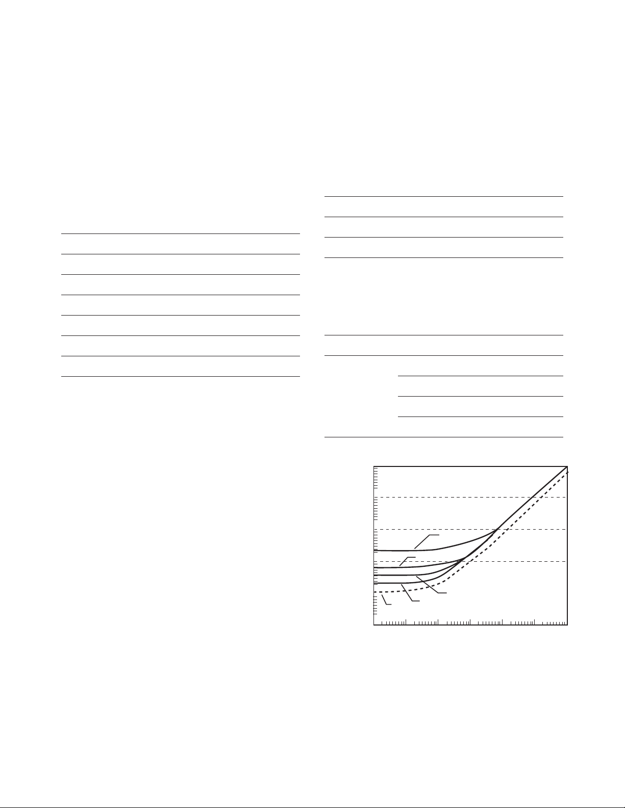
DC Bias Settling Time
When DC bias is set to on, add the settling time
listed in the following table to the measurement
time. This settling time does not include the DUT
charge time.
Bias current isolation
Test frequency (fm)On Off
20 Hz ≤ fm< 1 kHz 210 ms 20 ms
1 kHz ≤ fm< 10 kHz 70 ms 20 ms
10 kHz ≤ fm≤ 1 MHz 30 ms 20 ms
Sum of DC bias settling time plus DUT (capacitor)
charge time is shown in the following figure.
Bias source Bias current isolation Test frequency (fm)
(1) Standard On/Off 20 Hz ≤ fm≤ 1 MHz
(2) Option 4284A-001 Off 20 Hz ≤ fm≤ 1 MHz
(3) On 10 kHz ≤ fm≤ 1 MHz
(4) On 1 kHz ≤ fm< 10 kHz
(5) On 20 Hz ≤ fm< 1 kHz
100sec
10sec
1 sec
210msec
100msec
70msec
30msec
20msec
12msec
10msec
Setting time
1 mF 10 mF 100 mF1 µF 10 µF 100 µF
(1)
(2)
(3)
(5)
(4)
Capacitance
Figure 1-6. Measurement time
Page 18
18
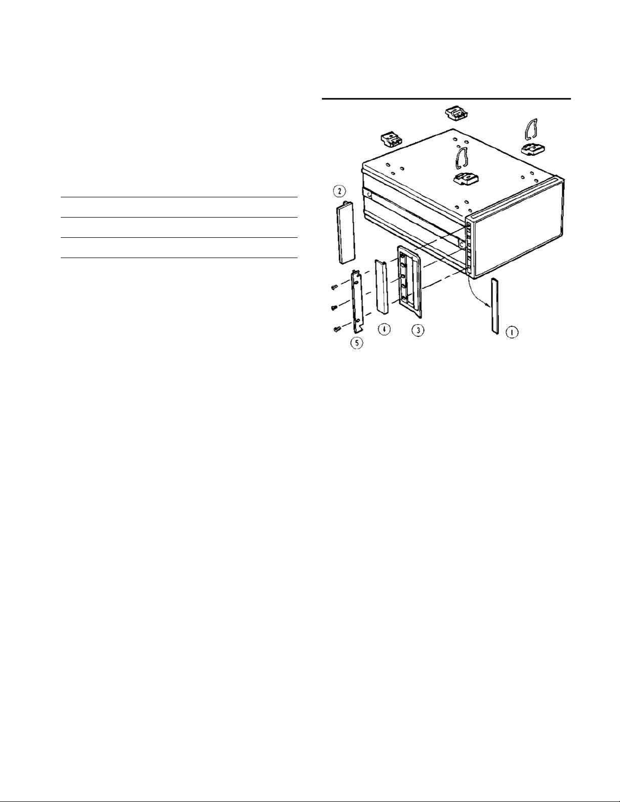
Rack/Handle Installation
The Agilent 4284A can be rack mounted and used
as a component of a measurement system. The following figure shows how to rack mount the 4284A.
Table 1-8. Rack mount kits
Option Description Kit part number
4284A-907 Handle kit 5061-9690
4284A-908 Rack flange kit 5061-9678
4284A-909 Rack flange and handle kit 5061-9684
Figure 1-7. Rack mount kits installation
1. Remove the adhesive-backed trim strips (1) from the left and
right front sides of the 4284A.
2. HANDLE INSTALLATION: Attach the front handles (3) to the
sides using the screws provided and attach the trim strip (4) to the
handle.
3. RACK MOUNTING: Attach the rack mount flange (2) to the left
and right front sides of the 4284A using the screws provided.
4. HANDLE AND RACK MOUNTING: Attach the front handle (3)
and the rack mount flange (5) together on the left and right front
sides of the 4284A using the screws provided.
5. When rack mounting the 4284A (3 and 4 above), remove all
four feet (lift bar on the inner side of the foot and slide the foot
toward the bar).
Page 19

19
Storage and repacking
This section describes the environment for storing
or shipping the Agilent 4284A, and how to repackage the 4284A far shipment when necessary.
Environment
The 4284A should be stored in a clean, dry environment. The following environmental limitations
apply for both storage and shipment
Temperature: –20 °C to 60 °C
Humidity: ≤ 95% RH (at 40 °C)
To prevent condensation from taking place on the
inside of the 4284A, protect the instrument against
temperature extremes.
Original packaging
Containers and packing materials identical to
those used in factory packaging are available
through your closest Agilent sales office. If the
instrument is being returned to Agilent for servicing, attach a tag indicating the service required,
the return address, the model number, and the full
serial number. Mark the container FRAGILE to
help ensure careful handling. In any correspondence, refer to the instrument by model number
and its full serial number.
Other packaging
The following general instructions should be
used when repacking with commercially available
materials:
1. Wrap the 4284A in heavy paper or plastic. When
shipping to an Agilent sales office or service
center, attach a tag indicating the service
required, return address, model number, and
the full serial number.
2. Use a strong shipping container. A doublewalled carton made of at least 350 pound test
material is adequate.
3. Use enough shock absorbing material (3- to
4-inch layer) around all sides of the instrument
to provide a firm cushion and to prevent movement inside the container. Use cardboard to
protect the front panel.
4. Securely seal the shipping container.
5. Mark the shipping container FRAGILE to help
ensure careful handling.
6. In any correspondence, refer to the 4284A by
model number and by its full serial number.
Caution
The memory card should be removed before
packing the 4284A.
Page 20

Agilent Technologies’ Test and Measurement Support, Services, and Assistance
Agilent Technologies aims to maximize the value you receive, while minimizing your
risk and problems. We strive to ensure that you get the test and measurement
capabilities you paid for and obtain the support you need. Our extensive support
resources and services can help you choose the right Agilent products for your
applications and apply them successfully. Every instrument and system we sell has
a global warranty. Support is available for at least five years beyond the production life
of the product. Two concepts underlie Agilent’s overall support policy: “Our Promise”
and “Your Advantage.”
Our Promise
Our Promise means your Agilent test and measurement equipment will meet its
advertised performance and functionality. When you are choosing new equipment, we will help you with product information, including realistic performance
specifications and practical recommendations from experienced test engineers.
When you receive your new Agilent equipment, we can help verify that it works
properly and help with initial product operation.
Your Advantage
Your Advantage means that Agilent offers a wide range of additional expert test
and measurement services, which you can purchase according to your unique technical and business needs. Solve problems efficiently and gain a competitive edge
by contracting with us for calibration, extra-cost upgrades, out-of-warranty repairs,
and onsite education and training, as well as design, system integration, project
management, and other professional engineering services. Experienced Agilent
engineers and technicians worldwide can help you maximize your productivity, optimize the return on investment of your Agilent instruments and systems, and obtain
dependable measurement accuracy for the life of those products.
www.agilent.com/find/emailupdates
Get the latest information on the products and applications you select.
Agilent T&M Software and Connectivity
Agilent’s Test and Measurement software and connectivity products, solutions and
developer network allows you to take time out of connecting your instruments to
your computer with tools based on PC standards, so you can focus on your tasks,
not on your connections. Visit
www.agilent.com/find/connectivity
for more information.
For more information on Agilent Technologies’ products, applications or services,
please contact your local Agilent office. The complete list is available at:
www.agilent.com/find/contactus
Product specifications and descriptions in this document subject to change
without notice.
© Agilent Technologies, Inc. 2004, 2003, 2002
Printed in USA, September 21, 2004
5963-5390E
Phone or Fax
United States:
(tel) 800 829 4444
(fax) 800 829 4433
Canada:
(tel) 877 894 4414
(fax) 800 746 4866
China:
(tel) 800 810 0189
(fax) 800 820 2816
Europe:
(tel) 31 20 547 2111
Japan:
(tel) (81) 426 56 7832
(fax) (81) 426 56 7840
Korea:
(tel) (080) 769 0800
(fax) (080)769 0900
Latin America:
(tel) (305) 269 7500
Ta iw a n :
(tel) 0800 047 866
(fax) 0800 286 331
Other Asia Pacific Countries:
(tel) (65) 6375 8100
(fax) (65) 6755 0042
Email: tm_ap@agilent.com
Agilent Email Updates
 Loading...