AEMC Instruments MTX 162UE, MTX 162UEW User manual

V

i

r

t

u

a

l

d

i

g

i

t

V

i

r

t

u

a

l

d

i

V

i

r

t

u

a

l

d

o

s

c

i

l

l

o

s

o

s

c

i

l

l

o

s

c

i

MTX 162UE

MTX 162UE

MT

X 162UEMTX 162UE

l

l

o

o

s

s

c

c

c

g

i

g

o

o

o

p

p

p

i

i

a

t

a

t

e

e

e

a

l

l

l

s

s

s

22 cchhaannnneell,, 6600 MMHHzz,, FFFFTT,, UUSSBB,, EEtthheerrnneet

MTX 162UEW

MTX 162UEW

MTX 162UEWMTX 162UEW

22 cchhaannnneell,, 6600 MMHHzz,, FFFFTT,, UUSSBB,, EEtthheerrnneett,, WWiiFFi

O

p

e

r

a

t

i

n

g

I

n

s

t

r

u

c

t

i

o

n

s

O

O

p

p

e

r

a

t

i

n

g

I

n

s

t

r

u

c

e

r

a

t

i

n

g

I

n

s

t

t

r

u

c

t

i

o

n

s

i

o

n

s

t..

i..

Pôle Test et Mesure de CHAUVIN-ARNOUX

Parc des Glaisins - 6, avenue du Pré de Challes

F - 74940 ANNECY-LE-VIEUX

Tel. [phone] - Fax [phone]

Copyright ©

Find Quality Products Online at: [e-mail]

www.GlobalTestSupply.com

X03409A00 - Ed. 01 - 12/09

Contents

Contents

Getting started Chapter I

Precautions and safety measures .................................... 5

Preparing for use ............................................................... 5

Maintenance .......................................................................6

Maintenance and metrology checks................................. 6

Communications interfaces .............................................. 6

Powering up ....................................................................... 6

Connection .........................................................................6

First use Chapter II

Command software .......................................................... 7

Installation........................................................................ 7

Launching ........................................................................ 7

First start-up....................................................................... 7

Control screen descriptions.............................................. 9

"Oscilloscope Control" ................................................... 9

"Oscilloscope Trace"....................................................... 9

Following start-ups Chapter III

Starting an oscilloscope................................................. 11

Starting an existing oscilloscope ................................. 11

Starting a new oscilloscope.......................................... 11

Our recommendations................................................... 11

Changing the IP address ................................................. 12

Pr

Starting a WiFi connection............................................ 15

Returning to USB cable connection ............................. 17

Returning to an ETHERNET cable connection ............ 18

Our recommendations................................................... 19

Updating the on-board software ..................................... 20

Our recommendations................................................... 21

Preliminary settings Chapter IV

Trace display mode......................................................... 22

Grid................................................................................. 22

Vertical scale ................................................................. 22

Vector representation, envelope, persistence ............22

Setting the trigger ............................................................ 23

Mode............................................................................... 23

Filter ............................................................................... 24

Source............................................................................ 24

Level.................................................

Tuning to a signal ........................................................... 25

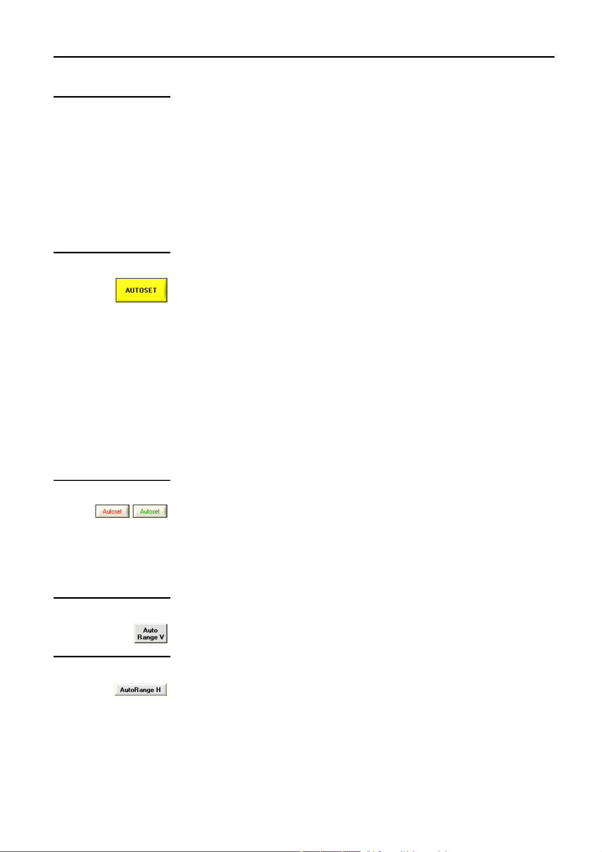
General autoset .......................................

Vertical autoset ............................................................. 25

Vertical autorange......................................................... 25

Horizontal autorange .................................................... 25

Find Quality Products Online at: [e-mail]

Manual settings ............................................................. 26

I - 2 Virtual digital oscilloscopes, 60 MHz

www.GlobalTestSupply.com

ogramming the WiFi connection ................................. 13

.............................. 24

...................... 25

Contents

Contents

Chapter V

Using the double time base: Zoom.......................................................................................... 27

Making measurements from the trace Chapter VI

Selecting the reference channel ..................................... 29

Manual measurements using the cursor........................ 30

An

Free cursors .................................................................. 31

Manual phase measurements....................................... 32

Automatic measurements ............................................... 33

General measurements on a channel .......................... 33

Automatic phase measurements ................................. 35

Carrying out specific processes Chapter VII

Min/Max high resolution acquisition............................... 36

Averaging the trace.......................................................... 36

Trace MATH...................................................................... 37

Calculating an FFT........................................................... 39

Starting an FFT calculation .......................................... 39

FFT settings................................................................... 40

Interpreting the FFT ...................................................... 41

Graphic representation................................................. 43

Exiting the FFT calculation........................................... 44

Obtaining an XY representation...................................... 45

Starting the XY representation........................

Using the trace .............................................................. 46

Cancelling the XY representation................................. 47

Capturing traces .............................................................. 48

Starting the capture ...................................................... 48

Using the data ............................................................... 49

Printing the capture ...................................................... 50

Exporting the capture to EXCEL .................................. 50

Cancelling trace capture............................................... 51

Freezing, Saving, Displaying the trace Chapter VIII

Freezing the trace ............................................................ 52

Saving the trace ............................................................... 53

Save .TRC ...................................................................... 53

Save .TXT....................................................................... 54

Displaying the trace ........................................................ 55

Memorizing, Retrieving the configuration Chapter IX

Memorising the configuration ................................. 56 - 57

Re

Find Quality Products Online at: [e-mail]

Virtual digital oscilloscopes, 60 MHz I - 3

(continued)

chored cursors ......................................................... 30

............. 45

calling the configuration ............................................ 58

www.GlobalTestSupply.com

Contents

Contents

Chapter X

Exporting the trace to EXCEL .................................................................................................. 59

Chapter XI

Technical specifications........................................................................................................... 62

Chapter XII

General, mechanical specifications......................................................................................... 68

Chapter XIII
Supplies

Accessories...................................................................... 69

shipped .......................................................................... 69

as options ..................................................................... 69

Index

(continued)

Attention !

Before printing this notice,

think of the impact on the

environment.

Find Quality Products Online at: [e-mail]

I - 4 Virtual digital oscilloscopes, 60 MHz

www.GlobalTestSupply.com

Getting started

Getting started

Congratulations!

Composition

Precautions and safety measures

Definition of the

measurement category

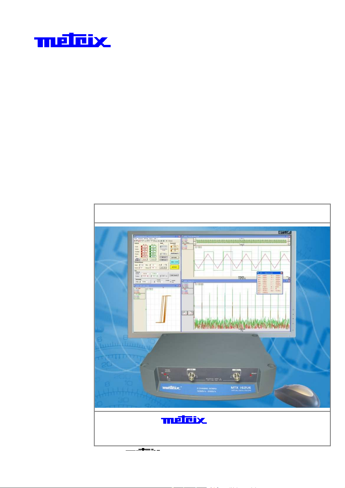
You have just purchased an MTX 162 oscilloscope. We thank you for your
confidence in our product quality.

This oscilloscope range is as follows:

MTX 162UE 2 channels, 60 MHz, 50 MS/s, 8 bits, 50 kpts, USB, Ethernet
MTX 162UEW 2 channels, 60 MHz, 50 MS/s, 8 bits, 50 kpts, USB, Ethernet, WiFi

The instrument complies with the safety standard NF EN 61010-1 (2001), single
insulation, relative to electronic measuring instruments.

In order to obtain the best results please read this notice carefully and follow the
precautions for use.

The failure to respect the warnings and/or usage instructions may damage the
appliance and can be dangerous for the user.

• oscilloscope 60 MHz, 2 channels, without display device

• software SCOPEin@BOX_LE to be installed on the "Host PC"

• safety instructions

- Indoor use

- Level 2 pollution environment

- Altitude below 2000 m

- Temperature between 0°C and 40°C

- Relative humidity less than 80% up to 31°C

- Measures on 300 V CAT II circuits, relative to the earth, can be supplied by a
240 V CAT II network.

CAT II: Category II measurements are those carried out on circuits directly
connected to the low voltage installation.
Example: supply of household appliances and portable electric tools

Preparing for use

before use

• Respect the environment and storage conditions.

• Make sure that the three wired phase/neutral/earth power cable delivered with

the appliance is in good condition. It is compliant with the NF EN 61010 (2001)
standard and must be connected to the instrument on the one side and to the
network on the other (variation from 90 to 264 VAC).

during use

• Read notes preceded by the symbol carefully.

• Connect the instrument to an earthed power outlet.

• Take care not to obstruct the ventilation.

• Only use the appropriate cables and accessories shipped with the appliance.

• When the appliance is connected to measurement circuits, never touch

an unused terminal.

Power supply The oscilloscope power supply is designed for a network varying from

90 to 264 VAC (nominal usage range: 100 to 240 VAC).
The frequency of this network must be between 47 and 63 Hz.

Symbols on

the instrument

Warning: danger hazard, consult the operating instructions.

Selective sorting of waste for recycling electrical and electronic equipment.
In compliance with the WEEE 2002/96/CE directive:
must not be considered as household waste.

Earth terminal

USB

Find Quality Products Online at: [e-mail]

European compliance

www.GlobalTestSupply.com

Virtual digital oscilloscopes, 60 MHz I - 5

Getting started (continued)

Getting started

Maintenance

Maintenance Metrology checks

Communication interfaces

USB V1.1 is an interface that connects the instrument directly to a PC USB port.

ETHERNET Depending on the oscilloscope equipment Ethernet can be connected:

Powering up

Connection

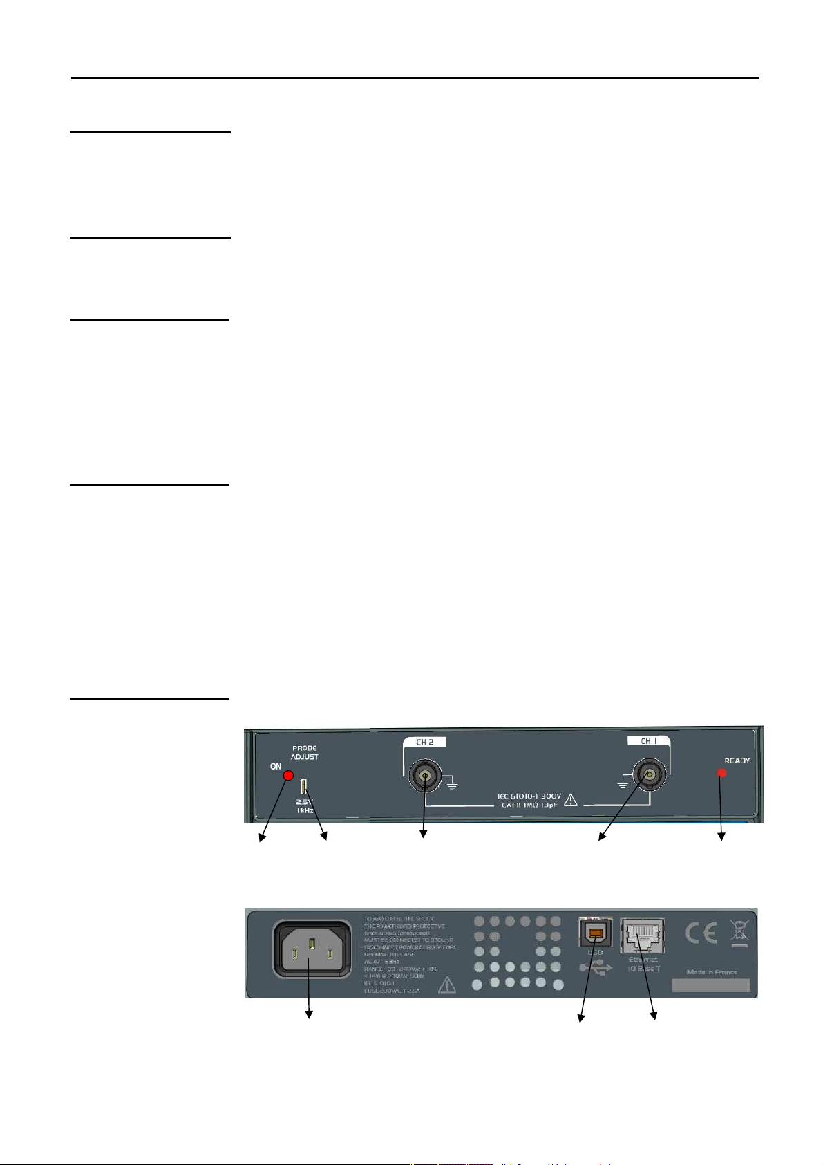
Terminal board

Oscilloscope is powered on

(connected to the power supply)

No interventions within the appliance are authorised.

- Power off the appliance (remove the power supply cable).

- Clean with a damp cloth and soap.

- Never use abrasive products or solvents.

- Dry quickly using a cloth or pulsed air at 80°C max.

The instrument has no elements that can be replaced by the operator.
All operations must be carried out by approved and competent staff.

For all repairs under guarantee or outside guarantee, please return the device to
your distributor.

Simple to use, no adjustments are needed for a local application.

- using a cable (straight cable for connection to a network or crossed
for local use)

- or wireless using WiFi (MTX 162UEW only).

Before powering up your oscilloscope and its connection to the Host-PC, insert the
supplied CD ROM and install the SCOPEin@BOX_LE driver software.

Then, connect the oscilloscope:

• either to the PC by USB using the supplied USB A/B cable

• or to the PC on the ETHERNET local network (point to point) using a

crossed ETHERNET cable

• or to the ETHERNET cable network using a straight ETHERNET cable

• if your oscilloscope has the WiFi option (MTX 162UEW), you must first configure

this connection mode before being able to use it (see chapter III).
Finally, connect the power supply cable to the power outlet and refer to the

following paragraphs.

Sensor

calibration

Entry for

CH2 channel

RJ45
ETHERNET

LED READY multifunction:

- availability of the appliance

- identification of the appliance

- search for the WiFi network

Back face

Find Quality Products Online at: [e-mail]

Power socket

www.GlobalTestSupply.com

USB

connector

RNET Connector

I - 6 Virtual digital oscilloscopes, 60 MHz

First use

by using USB, or ETHERNET (RJ45 cable or

First use

Command software

Installation Carefully read the safety instructions shipped with the instrument and

Launching When the oscilloscope's "READY" LED lights, you can launch the

First start-up

The command software is SCOPEin@BOX_LE.exe :

insert the CDROM in your PC CD drive.

SCOPEin@BOX_LE.exe software.

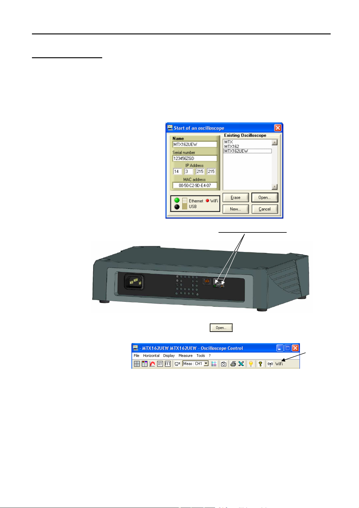
At first start-up the following windows are opened:

Enter a "name" for the instrument (by default MTX
162 is selected); the instrument configuration files
will be associated to this name.

Restarts a search for connected instruments

launches online help for this window.

The SCOPEin@BOX_LE software automatically
searches for MTX 162 oscilloscopes connected to
the PC
WiFi if equipped).
It then displays the list of these instruments with, for
each one:

- its generic name,

- the onboard software version

- the serial number.

The selected MTX 162 oscilloscope's IP address
and the PC's address are displayed.

 Press the key to refresh the display if your oscilloscope does

not appear in the list of connected instruments.
If this fails, check your instrument's connection and/or re-start it
by disconnecting and reconnecting it to the power supply.

1. Name your instrument.

2. Select one of the instruments connected to the PC (via USB or
ETHERNET) from the proposed lists.

3. Click on the button to create and launch the instrument.

 In our example we are starting up the "MTX 162UEW"

oscilloscope for the first time.
By default the instrument's IP address is 192.168.0.100 (with the

55.255.255.0 network mask).

2
The instrument's IP address must therefore be adapted to the

network address used by the host-PC (here: 14.3.212.31).

Find Quality Products Online at: [e-mail]

Virtual digital oscilloscopes, 60 MHz II - 7

www.GlobalTestSupply.com

First use

First use (continued)

First start-up
(continued...)

The selection of an instrument connected using Ethernet leads to the
display of the following window if the IP address, entered by default, is not
compatible with the network to which the PC is connected:

To avoid IP address conflicts on the network you are using, consult
your administrator in order to select an available address that is
compatible with the network.

In our example the network mask used is 255.255.0.0; we program our

IP address: 14.3.215.215 and validate the entry using the key.

The IP address is tested on validation to make sure that the entered
address is not already used on the network.

If the result is correct the instrument starts up.

Find Quality Products Online at: [e-mail]

II - 8 Virtual digital oscilloscopes, 60 MHz

www.GlobalTestSupply.com

First use

Specific settings for

Mathematical

Trigger parameter

calculation

First use (continued)

Control screen descriptions

"Oscilloscope

Control"

channels CH1 & CH2

Menu bar

Tool bar

functions

settings

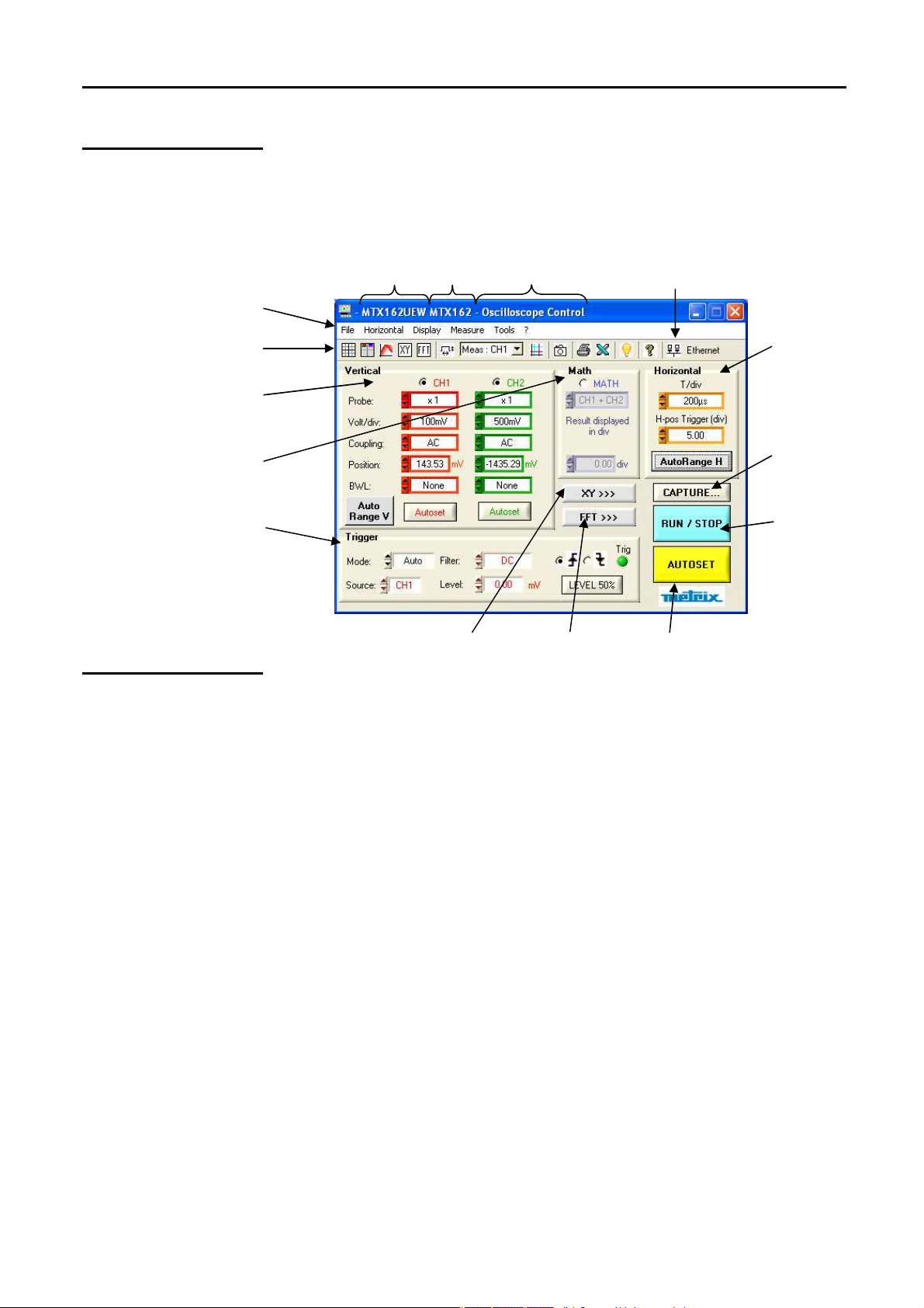
When the instrument is launched the "Oscilloscope Control" and
"Oscilloscope Trace" should be displayed.

This window contains all the possible settings for the oscilloscope:

Type of instrument

Instrument

name

Window name

Current

communications mode

Horizontal scale
settings

Trace capture

Acquisition
Start/stop

"Oscilloscope

Trace"

Activate XY

representation

Activation of

FFT

Launch general

autoset

This window contains the graphical representation of the signals:

• 2500 points per channel are used to display curves.

They are sent from the oscilloscope to the PC via the communications
interface (USB / ETHERNET / ETHERNET WiFi).

These 2500 points are different depending on the activation or not of
the FFT calculation:

- when FFT is not active,

to avoid erroneous graphical representations related to the selection of
one point in 20 (the acquisition memory being 50 000 points), the 2500
points sent to the PC are in fact 1250 couples (min, max) of the
extreme values encountered in each 40 point interval in the acquisition
memory.

- when FFT is active,

the points that are sent are also used in the Fourier transformation and
the use of the couples (min, max) would lead to an erroneous
frequency representation.
They are therefore obtained using a basic decimation (1 point every

20) of the content of the acquisition memory. Erroneous temporal
representations on the screen are therefore possible.

• if the zoom is activated, 2500 additional points are sent (double time

base).

These 2500 points are generally couples (Min, Max) except for when

he zoom is at its maximum and the 2500 viewed points correspond to

t
a continuous series of points from the acquisition memory.

Find Quality Products Online at: [e-mail]

Virtual digital oscilloscopes, 60 MHz II - 9

www.GlobalTestSupply.com

First use

First use (continued)

"Oscilloscope

Trace"

Indication of the vertical

sc

ale and the channel

coupling, if the function is

0V origin of the CH1 &

Acquisition time base

Information relative to

activated

CH2 traces

fixed traces,

if activated

This window contains the graphical representation of the signals:

Indication of averaging, if

activated

Grid, if

activated

Zoom

activation

Acquisition status:
LOADING: communication with the scope
RUN: currently acquiring
PRE-TRIG: currently loading pretrig
READY : pretrig loaded, waiting for trigger
POST-TRIG: currently loading post-trig
STOP: acquisition stopped

Position of the trigger
(of the source colour:
red = CH1, green = CH2,
brown = LINE) .
Different display depending
on the selected trigger filter:
T (DC)
TAC (AC)
THF (
TLF (LF reject)

Indicator for horizontal
and/or vertical
autorange activation

Authorise the
displacement of the
trigger using the
mouse or not

HF reject)

The display acquisition status is that at the moment o



of the points. The acquisition being totally asynchronous to the
display, it is possible that not every status be displayed in the
window.

f the transfer

Find Quality Products Online at: [e-mail]

www.GlobalTestSupply.com

II - 10 Virtual digital oscilloscopes, 60 MHz

Following start-ups

Information relative to the

al modes are shown by

green LEDs

the selected instrument

Following start-ups

Starting an oscilloscope

Selection of the communication mode.

The function

(LED lights = connection established).

Starting an existing

illoscope

osc

For the following start-ups the SCOPEin@BOX_LE firmware starts up
showing the "Start an oscilloscope" window:

selected instrument

(here MTX)

Selection
of the oscilloscope
and the corresponding
configuration

Deletion of

Create a new oscilloscope

The LED is red if the Ethernet

communication uses WiFi

Start-up of
the selected instrument

Exit the application

1. Select the oscilloscope in the 'Existing Oscilloscope' window.
The information relative to this instrument is displayed in the left part of
the window.

Starting a new

illoscope

osc

recommendations

Our

2. Check that the selected communication mode is operational: the
associated green LED must be lit.

3. Start the instrument by clicking on

 To easily identify the instrument, the selection of the oscilloscope

(click on its name) makes the red "READY" LED on the instrument
blink (unless communications with the instrument cannot be
established).

Use the key to open the "Create a new instrument" window
(see chapter II, §. First start-up).

If a communications mode is not operational:

• Make sure that the instrument is connected: disconnect the cables (USB

and Ethernet) and reconnect them.

• For driving using Ethernet check that the cable used is adapted to the

type of connection you wish to make (the green Ethernet RJ45
connector LED lights if the connection is operational):

- Straight-thru cable for connection to a company network

- crossover cable for a local connection to the PC

 Recent network cards accept a straight-thru cable for a direct

"instrument to PC" connection.

Find Quality Products Online at: [e-mail]

Virtual digital oscilloscopes, 60 MHz III - 11

www.GlobalTestSupply.com

Following start-ups

Following start-ups (continued)

recommendations

(continued)

Changing the IP address

Our

For Ethernet, make sure that:

• the IP address in the configuration file is the same as the address

programmed in the oscilloscope: click on and find your
instrument in the list of connected devices, or start-up the
instrument using USB; check the network parameters using the
Tools menu (see below).

• the oscilloscope's IP address is not already used on the network

and does not cause an addressing conflict:

- disconnect the network cable from the oscilloscope, run a 'ping <IP
address>’ command from your DOS Command screen (menu
'Start/Run…’ and open 'cmd').
If an instrument responds, change the IP address.

- If the problem persists, close the SCOPEin@BOX_LE application,
disconnect it, then reconnect the power supply on the MTX 162 to
reinitialise it.
When the "READY” LED lights, re-launch the application.

The IP address can be changed from the Tools 
"Oscilloscope Control" window:

 Network… menu in the



The key gives access to the network mask and gateway
programming.

Once the new IP address has been entered click on to validate it.
The address is then controlled before programming to make sure that the
entered address is compatible with the network and is not currently in use.

If the instrument is driven via Ethernet, the connection
reinitialized using the new address settings.

is stopped and

Find Quality Products Online at: [e-mail]

III - 12 Virtual digital oscilloscopes, 60 MHz

www.GlobalTestSupply.com

Following start-ups

Following start-ups (continued)

Programming the WiFi connection

Only the MTX 162UEW versions have the wireless communication option:
WiFi.

This WiFi function is compatible with the IEEE 802.11b and g wireless
communications standards, and for security it is compatible with the 802.11i
Encryption standard.

The MTX 162UEW can be used in one of the network topologies described
by this standard:

- the infrastructure topology, in which wireless clients are connected to
an access point that permits the interconnection of this wireless network
to a cabled network.

- the Ad Hoc topology, in which the clients are connected to each other
without any access points. This mode makes it possible, for example, to
connect one or more oscilloscopes directly to a PC.

It is strongly recommended that you protect your netwo
encryption and authentication mechanism, the MTX 162UEW manages the
WEP (64 and 128 bits), WPA and WPA2 security modes.
The latter two are to be privileged in terms of security.

However, when in Ad Hoc mode, only WEP security is supported.

The MTX 162UEW operates in roaming mode. It is therefore capable, in an
adapted network, (that has several access points with the same network
name (SSID) and the same security characteristics), of automatically
switching to the access point that has the greatest transmission power.

rk using a data

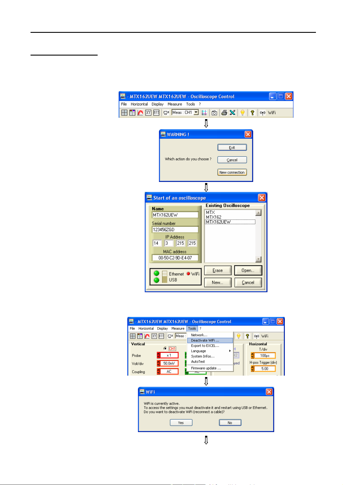
The WIFi settings cannot be changed if the device is using this
communication method. It is therefore necessary to return to a cable
connection first (USB or Ethernet).

If the oscilloscope is currently in WiFi mode it can b
'Tools' menu:

To continue, connect one of the communication cables to your oscilloscope
and click on

to start a new connection.

e connected using the

Find Quality Products Online at: [e-mail]

Virtual digital oscilloscopes, 60 MHz III - 13

www.GlobalTestSupply.com

Following start-ups

Programming the WiFi

Reception level

Access p

oint SSID

Following start-ups (continued)

connection
(continued)

Programming can also be carried out from the 'Tools 
menu in the 'Oscilloscope Control' window (this menu is greyed out for
instruments that are not equipped with the WiFi function).

Current instrument Ethernet

address

 Activate WiFi …’



To program the WiFi settings, refer to your wireless access point
documentation and copy its programming on the MTX 162UEW.

 The password cannot be re-read; it is only reprogrammed if the '

ASCII Key’, 'Hex Key’ or 'Phrase’ fields are changed.

used to test the reception level of the access point of which the SSID was
entered in the 'Network Name’ field. It shows the following window:

MAC address
for the access
point

Network topology:

I: infrastructure

A: Ad Hoc

Find Quality Products Online at: [e-mail]

III - 14 Virtual digital oscilloscopes, 60 MHz

www.GlobalTestSupply.com

Used WiFi channel

Security mode

Following start-ups

Following start-ups (continued)

Programming the WiFi
connection (cont.)

Activates the connection

Display of the "factory" settings with in order to completely reprogram the
oscilloscope. The default configuration is an Ad-Hoc non secured connection
with the MTX162 SSID.

This key is only accessible if one of the WiFi settings is changed;
it sends the values entered to the oscilloscope to be memorized.
Only the modified fields are programmed.

Launch of a new WiFi connection with the current settings (last values

memorised by pressing ).
If some settings are changed but not programmed the following message is

displayed:

after having sent the

settings to the

oscilloscope.

Activates the connection without taking

into account the changes to the WiFi

settings.

Return to the previous screen

without any action.

Starting a WiFi

connection

closes the window.

The WiFi connection starts in several ways:

When powering on

:

- if the instrument was using WiFi mode when it was powered off, the
oscilloscope will restart by attempting to establish the previous WiFi
connection.

- if not, if no cables (USB or Ethernet) are connected to the instrument, a
search for a WiFi connection is begun using the current settings.

Cable operation (USB or Ethernet):

- if no WiFi is already operational, from the 'Tools 

 Activate WiFi…’



menu in the 'Oscilloscope Control’ window.

Then in the WiFi’ window (see above), click on

. A new WiFi

session opens automatically if the connection is correctly established.

- if a WiFi connection is already established (the 'Tools 

iFi…’ menu is displayed), by closing the application and opening a new

W

 Deactivate



connection from the 'Start of an Oscilloscope' window.

Find Quality Products Online at: [e-mail]

Virtual digital oscilloscopes, 60 MHz III - 15

www.GlobalTestSupply.com

Following start-ups

Following start-ups (continued)

Starting a WiFi

connection

(continued)

The search for a WiFi network is visible on the front face of the instrument;
the "READY" LED will rapidly blink for 40 blinks.

A maximum of 10 rapid blinks are shown; if the "READY" LED is permanently lit
before the 10 rapid blinks, the connection is established, otherwise the search
for an Ethernet cable connection is activated.

If successful the "WiFi" LED in the 'Start of an oscilloscope" window lights
in red:

On the rear face of the instrument, the green and yellow LEDs

for the RJ45

network are lit:

Select 'Ethernet WiFi’ and click on to start the instrument using

i.

WiF

WiFi
communication ...

Find Quality Products Online at: [e-mail]

III - 16 Virtual digital oscilloscopes, 60 MHz

www.GlobalTestSupply.com

Following start-ups

Following start-ups (continued)

Returning to

an USB cable

communication

Two methods are possible:

Connect the USB cable between the device and the PC, then:

- to keep the WiFi connection:

Select the USB and open the new connection.

- to abandon the WiFi connection:

Find Quality Products Online at: [e-mail]

Virtual digital oscilloscopes, 60 MHz III - 17

www.GlobalTestSupply.com

Following start-ups

Following start-ups (continued)

Returning to a USB

cable

communication

(continued)

Select the USB and open the new connection.

Returning to

an ETHERNET

cable connection

Connect the Ethernet cable, then:

Select Ethernet and open the new connection.

Find Quality Products Online at: [e-mail]

III - 18 Virtual digital oscilloscopes, 60 MHz

www.GlobalTestSupply.com

Following start-ups

Following start-ups (continued)

Our

If the WiFi connection is not operational in the 'Start of an oscilloscope'

recommendations

window:

- Make sure that the WiFi connection settings for your oscilloscope are
identical to those programmed on your wireless access point.

- Use the key in the WiFi programming window, to assess the
reception level and, if needed, move your MTX 162UEW oscilloscope
closer to your access point in order to check whether you have a range
problem.

- Make sure (especially when switching from Ad Hoc / Infrastructure)
that the oscilloscope's IP address is compatible with the rest of the
equipment.

- For use in an Ad Hoc topology (PC + MTX 162UEW), it is imperative
to establish the Ad Hoc connection on your PC before starting the
network search on the oscilloscope (powering on the oscilloscope).

Find Quality Products Online at: [e-mail]

Virtual digital oscilloscopes, 60 MHz III - 19

www.GlobalTestSupply.com

Following start-ups

Select a

file

Open the update window

Following start-ups (continued)

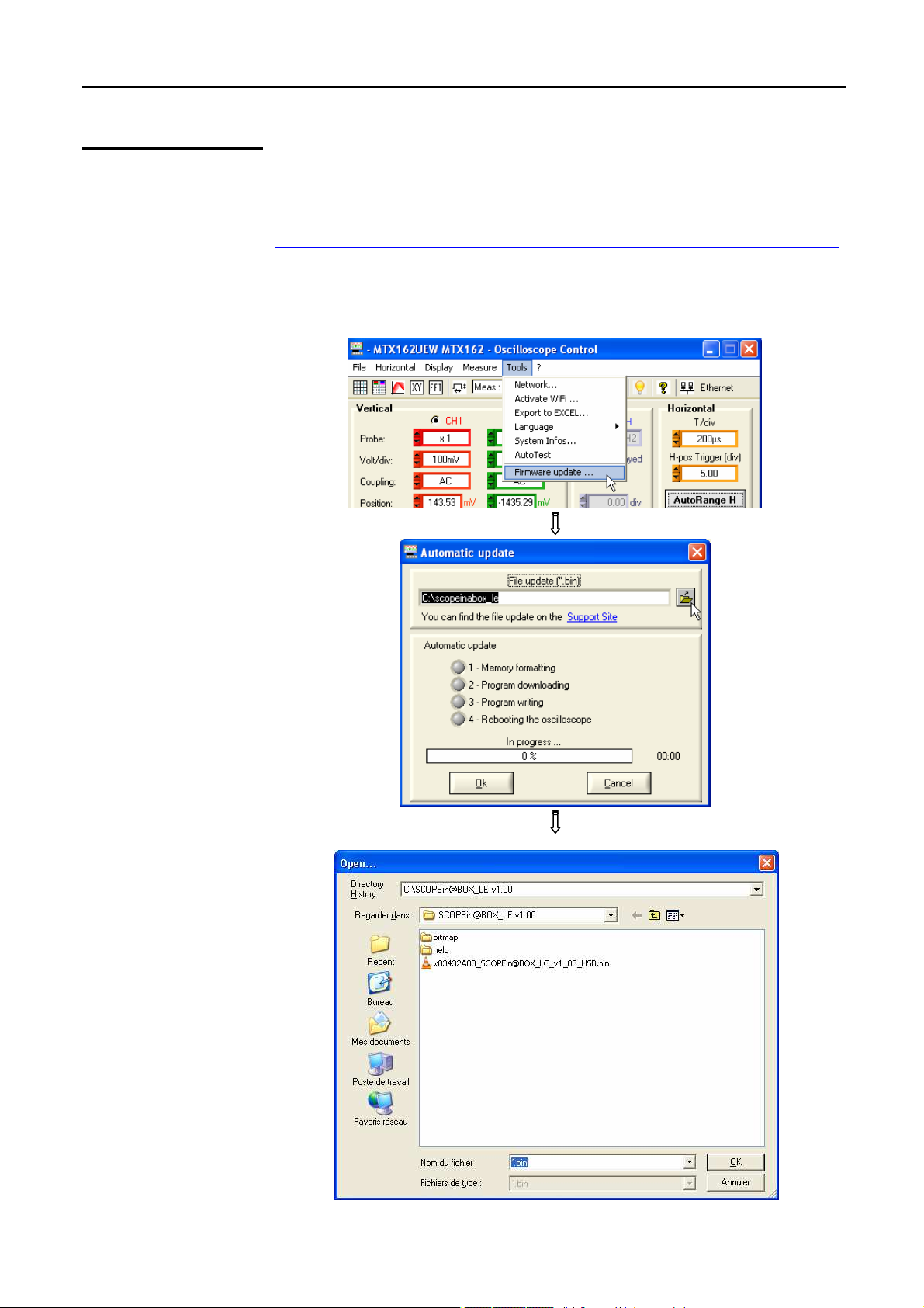
Updating the on­board firmware

The update of the internal MTX 162 firmware is made using a ".BIN" file
that you can download from our technical support web site at the following
address:

http://www.chauvin-arnoux.com/SUNSUPPORT/SUPPORT/page/pageSupportLog.asp

We recommend that you place this file in the application's work directory
(by default: c:\SCOPEin@BOX_LE).

This file is used in the 'Tools’ menu of the 'Oscilloscope Control' window:

Find Quality Products Online at: [e-mail]

III - 20 Virtual digital oscilloscopes, 60 MHz

www.GlobalTestSupply.com

Following start-ups

Following start-ups (continued)

Access

recommendations

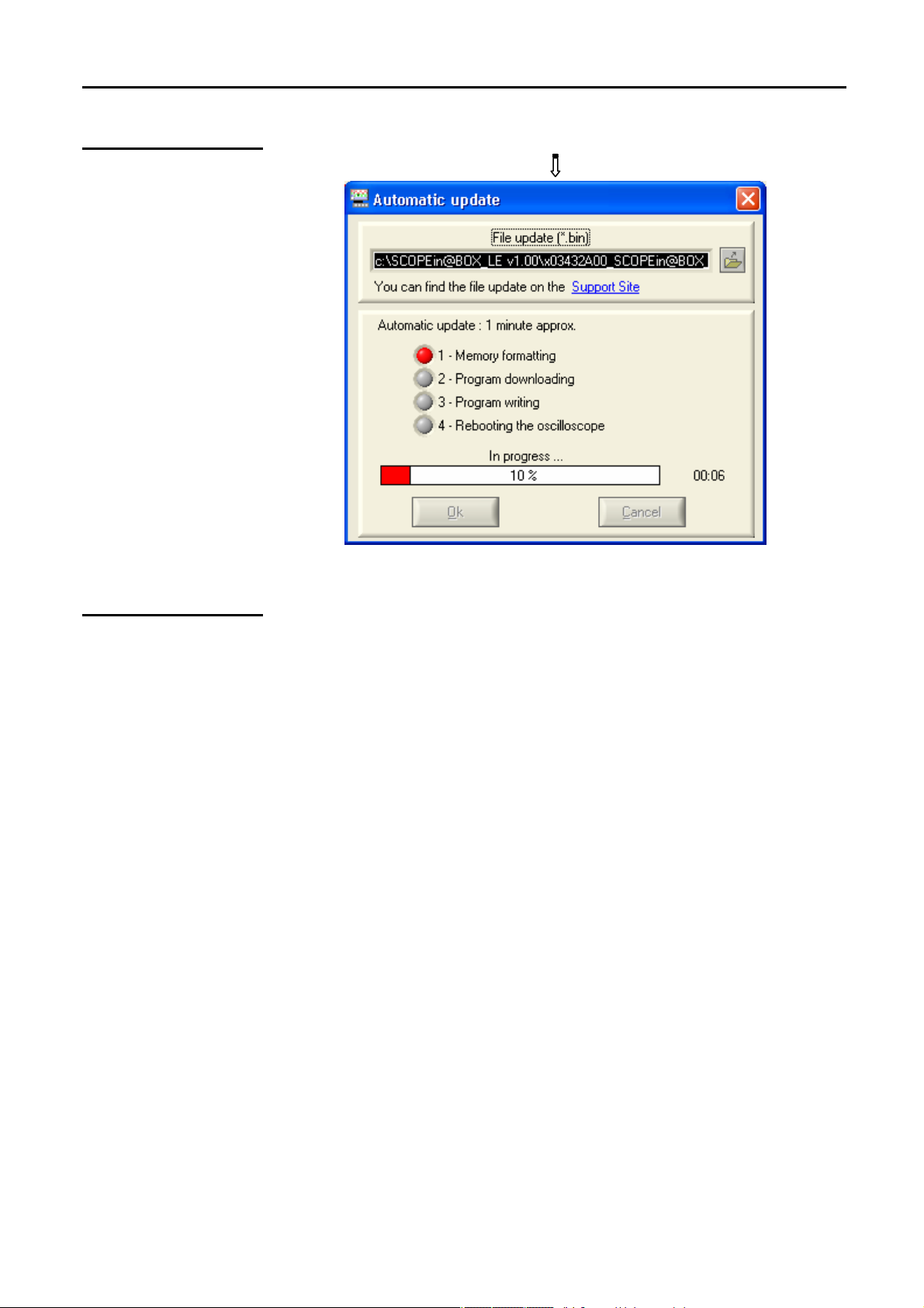
The download successfully terminates 
automatically (after having forced the reinitialisation of the MTX 162).

Our

In the event of an error, renew the update operation.

If your instrument has not re-initialised correctly, close the
SCOPEin@BOX_LE application and re-initialise the MTX 162 by
disconnecting it from the power supply.

The update is secure and cannot cause the destruction of the onboard
MTX 162 firmware.

In the worst case the update can continue during the next start-up and thus
lengthen the start-up time. The time needed to finish the installation cannot
be greater than two minutes.

After this amount of time, reinitialise the MTX 162 by disconnecting the
power supply.

 the application re-starts



Find Quality Products Online at: [e-mail]

Virtual digital oscilloscopes, 60 MHz III - 21

www.GlobalTestSupply.com

Preliminary settings

Trace display mode

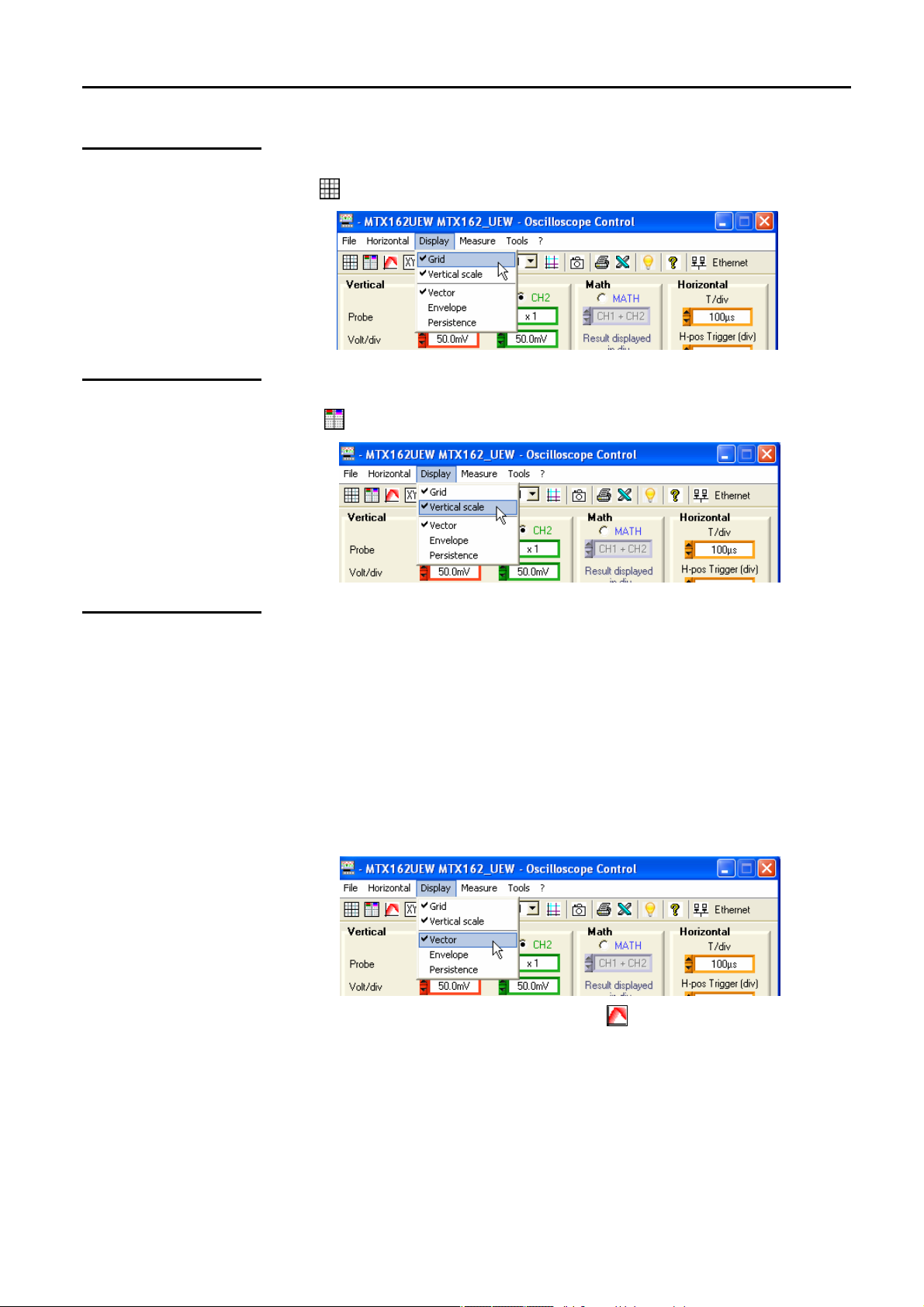
Grid

Vertical scale

You can choose to display or hide the grid in the trace windows by clicking
on the in the tool bar or from the menu:

The vertical trace scale can be inserted into the trace windows by clicking
on the button in the tool bar or from the menu:

Vector representation, Envelope or Persistence

The 'Vector' representation is the most classical since it consists in linking
each pair of samples by a segment.

The 'Envelope' traces the envelope of Min/Max samples keeping, for each
abscissa, the minimums and maximums displayed since the last time
acquisition was run.

'Persistence' simulates the analogue persistence of the displays on cathode
tube screens by keeping the 8 last traces for each channel, the brightness
of the colour shows the age (the brightest colour shows the most recent
trace).

To select one of these display modes click on the corresponding line:

Persistence can also be activated using the button in the tool bar.

Find Quality Products Online at: [e-mail]

IV - 22 Virtual digital oscilloscopes, 60 MHz

www.GlobalTestSupply.com

Preliminary settings

Setting the trigger

Mode

Auto

The trigger is essential to obtain a correct representation of the signal.

Its setting is made using 5 settings that can be accessed from the
"Oscilloscope control" window which are:

• the mode

• the filter

• the front selection

• the source

• the level

The Trig LED on this block shows the presence of triggering events.

4 trigger modes are available:

for automatic; this mode guarantees signal acquisition even in the absence
of trigger conditions. If no pulse is detected for approximately 500 ms, the
oscilloscope switches to automatic triggering and regularly, with a period <
80 ms, generates virtual triggers making it possible to have acquisition If
pulses are detected (signal frequency > Hz and level correctly adjusted),
the automatic mode operates as the triggered mode.

 When the oscilloscope switches to triggered mode (without trigger

signal), the trace is no longer stabilised on the screen, the
averaging of the "envelope" modes, if they are triggered, can then
give erroneous representations and erroneous automatic
measurements.

Trig

Mono

for "triggered"; in this mode each detection of a trigger event (ascending or
descending wave) on the signal selected as the source, causes a trigger
that makes it possible to complete the current acquisition. A new acquisition
is immediately begun to anticipate the next trigger event. In the absence of
a signal the acquisition is not completed ('Ready' status), the trace is not,
therefore, displayed.

for single; a single acquisition is run and continues until a trigger event is
detected.

Pressing on resets the trigger for a new acquisition.

 Trigger events are only taken into account once the Pretrig phase

is complete (filling of the memory between the origin of the window
and the trigger's horizontal position). A horizontal positioning of
the trigger on the left of the screen is used to reduce the
acquisition time.

Roll

Find Quality Products Online at: [e-mail]

Virtual digital oscilloscopes, 60 MHz IV - 23

This mode is used to view slow signals continuously. The acquisition here is
infinite and therefore does not require the setting of any trigger events. This

mode is limited to time bases ≥

coupling to DC (the AC coupling is not adapted to slow signals).

200 ms and forces the channel entry

≥

≥≥

www.GlobalTestSupply.com

Preliminary settings

Setting the trigger (continued)

Filter

Source

To limit false triggers or to adapt to a signal that is used as a trigger
source 4 filters are available:

AC cuts the continuous component of the signal (see remark below).

DC

lets the signal pass without filtering (the continuous and alternative
components are kept).

LF Reject activates a high-pass filter (cut-off frequency 10 kHz).

HF Reject activates a low-pass filter (cut-off frequency 10 kHz).



The coupling of the channel, selected in the vertical block of the
control panel is input to the acquisition string.
Consequently, if the AC input coupling is selected, the DC component
of the signal is removed on the CHx channel and on the trigger source
CHx (the AC or DC filtering of the trigger gives the same result).

3 trigger sources are available: CH1, CH2 and LINE.

LINE is used to trigger on the power supply voltage to which the instrument
is connected. In this case only the trigger wave (ascending or descending)
can be programmed.
The trigger representation on the trace is a vertical blue line,
the notion of level (vertical position) is no longer available.

Level

Adjustment of the trigger level by ± 8 div. to make sure it cuts this level with a
wave.

The
peak value of the source signal. This is not a general autoset that is capable
of finding the trigger, it only applies to the displayed signal.

key is used to reset the trigger level to 50 % of the peak to

Find Quality Products Online at: [e-mail]

IV - 24 Virtual digital oscilloscopes, 60 MHz

www.GlobalTestSupply.com

Preliminary settings

Signal settings

General autoset

As with a traditional oscilloscope, the correct representation of a signal
necessitates making a number of adjustments:

• Choice of the channel

• Trigger

• Time base

• Vertical sensitivity

• etc. …

Your oscilloscope proposes different strategies in order to obtain these
adjustments in the best conditions.

It defines all the instrument settings including the search for a signal on all
channels, the trigger settings and the time base. The signal frequency must

be ≥

≥ 20 Hz for the autoset to succeed.

≥≥

This action has a momentary effect after which it is possible to take over
manually using the classical commands.

 When the autoset succeeds it overwrites all the current settings.

Otherwise it has no effect on the current settings.

When 2 signals with different frequencies are present on the inputs, the
trigger is forced on the lowest frequency signal and the time base is
adapted to this signal.

Vertical autoset

Vertical autorange

Horizontal autorange

By default the time base is calculated in order to view at least 3 signal
periods. If the FFT is activated the time base is calculated so that the
fundamental of the frequency representation is at approximately one
division from the origin of the frequencies.

This command is specific to the associated channel (CH1 or CH2).

It activates the channel, adjusts sensitivity, offset, coupling (if DC coupling
is selected and offset is possible) to better adapt to the trace display.

It is a momentary action.

 When vertical autoset succeeds it overwrites the current settings.

If it fails the channel remains selected with its initial settings.

This function permanently adjusts the sensitivity on the signal amplitude on
condition that the signal's points have been acquired (select the AUTO
trigger mode if there is no trigger).

This function only works on the channel selected as the trigger source. It
permanently searches for the time base which is best adapted to view this
trace (display of at least 2 periods on the screen).

Find Quality Products Online at: [e-mail]

Virtual digital oscilloscopes, 60 MHz IV - 25

www.GlobalTestSupply.com

Preliminary settings

Signal settings (continued)

Manual settings

otherwise

The right approach consists in knowing the approximate specifications of the
signal to be analysed: frequency, amplitude.

In this case the time base and the vertical attenuator can be pre-set and the
trigger can be parametered.

- Select the AUTO trigger mode

- Validate the channel corresponding to the signal connection

- Choose the corresponding trigger source

- Select: Coupling Trigger AC

Level Trigger at 0 V
Sensitivity from 5 mV/div.

- Time base: find a sweep rate value that allows the display of several

complete periods.

 Refine the sensitivity to obtain an amplitude represent

without overlaps and, if necessary, the time base and the trigger
threshold.

ation

Find Quality Products Online at: [e-mail]

IV - 26 Virtual digital oscilloscopes, 60 MHz

www.GlobalTestSupply.com

Using the double time base: Zoom

zone

zone

position

Using the double time base: Zoom

To ease the use of acquisitions, a real time zoom is available on the
oscilloscope. It is used to observe a single signal using two different time
bases.

A click on the button of the "Oscilloscope Trace" window activates the
Zoom mode.

 This mode is switched to automatically for a time base lower

than 100 ns/div.

The "Oscilloscope Trace" window becomes:

Offset of 1div

zoomed

to the left

Graph of the

entire

acquisition depth

Zoomed

Horizontal

trigger

Offset of 8 divs

zoomed to the left

Graph

of the zoomed

Vertical

trigger

position

Offset of 1div
zoomed
to the right

Offset of
8 divs. zoomed
to the right

Acquisition
time base

Trigger
position relative
to the zoomed
zone

Vertical

zoomed scale

Zoom

increase

Exit zoom

It is possible to move the zoomed zone using the mouse by moving the
black frame to the left or to the right (keep the mouse clicked while

, , or .

moving the frame) or by using the buttons shown opposite.

Zoom

decrease

Find Quality Products Online at: [e-mail]

Virtual digital oscilloscopes, 60 MHz V - 27

www.GlobalTestSupply.com

Using the double time base: Zoom

zoomed zone

Using the double time base: Zoom (continued)

If the trigger is no longer in the zoomed zone its representation on the
zoomed graph becomes:

The trigger is to

e right of the

th

Find Quality Products Online at: [e-mail]

V - 28 Virtual digital oscilloscopes, 60 MHz

www.GlobalTestSupply.com

Making measurements from the trace

Making measurements from the trace

Selecting the reference channel

Once the representation of the traces has been obtained a more in-depth
analysis of the signals can be undertaken by making a few measurements
on the signal.

Two categories of measurements can be made using the MTX 162:

1. manual measurement using the cursors

2. automatic measurements

In both cases the measurements are made on the channel that was
selected as the reference.

It is selected:

• either from the tool bar in the selector

• or from the 'Measurement’ menu as follows:

.

Find Quality Products Online at: [e-mail]

Virtual digital oscilloscopes, 60 MHz VI - 29

www.GlobalTestSupply.com

Making measurements from the trace

abscissa

Making measurements from the trace (continued)

1. Manual measurements using the cursors

a) Snap to Point

measurements

These measurements are made on the 2500 points used for the display.

If the Zoom is active the cursors are available on the zoomed graph.

In this mode the cursors are attached to the trace for the channel defined
as the measurement reference: the user can only move them on the
horizontal axis.

A click on the button of the tool bar or on the 'Measure’ menu function
activates/deactivates the cursors:

Cursor 1 & 2

Variation of

abscissa dX = X 2

Channel to which

the cursors are

attached

The values of the
CH1 signal at the

X1 & X2 abscissa

Difference in

values

dY = Y2 - Y1

The 'Snap to Point measurements’ are driven from the "Oscilloscope
Trace" window which becomes:

Origin of the time

base

Cursor 1 Cursor 2

Find Quality Products Online at: [e-mail]

VI - 30 Virtual digital oscilloscopes, 60 MHz

www.GlobalTestSupply.com

Making measurements from the trace

abscissa

Making measurements from the trace (continued)

b) Free cursors

Cursor 1 & 2

Variation of abscissa

dX = X2 - X1

Using this mode the user is free to position the cursors at will on the
graph. The position of each cursor is given following the vertical scale of
the different traces.

These measurements were selected from the 'Measure’ menu:

The "Oscilloscope Trace" window becomes:

Cursor 1

Cursor 2

Y-axis values of the

cursors following the

vertical scale

of channel CHX

Find Quality Products Online at: [e-mail]

Virtual digital oscilloscopes, 60 MHz VI - 31

www.GlobalTestSupply.com

Making measurements from the trace

Making measurements from the trace (continued)

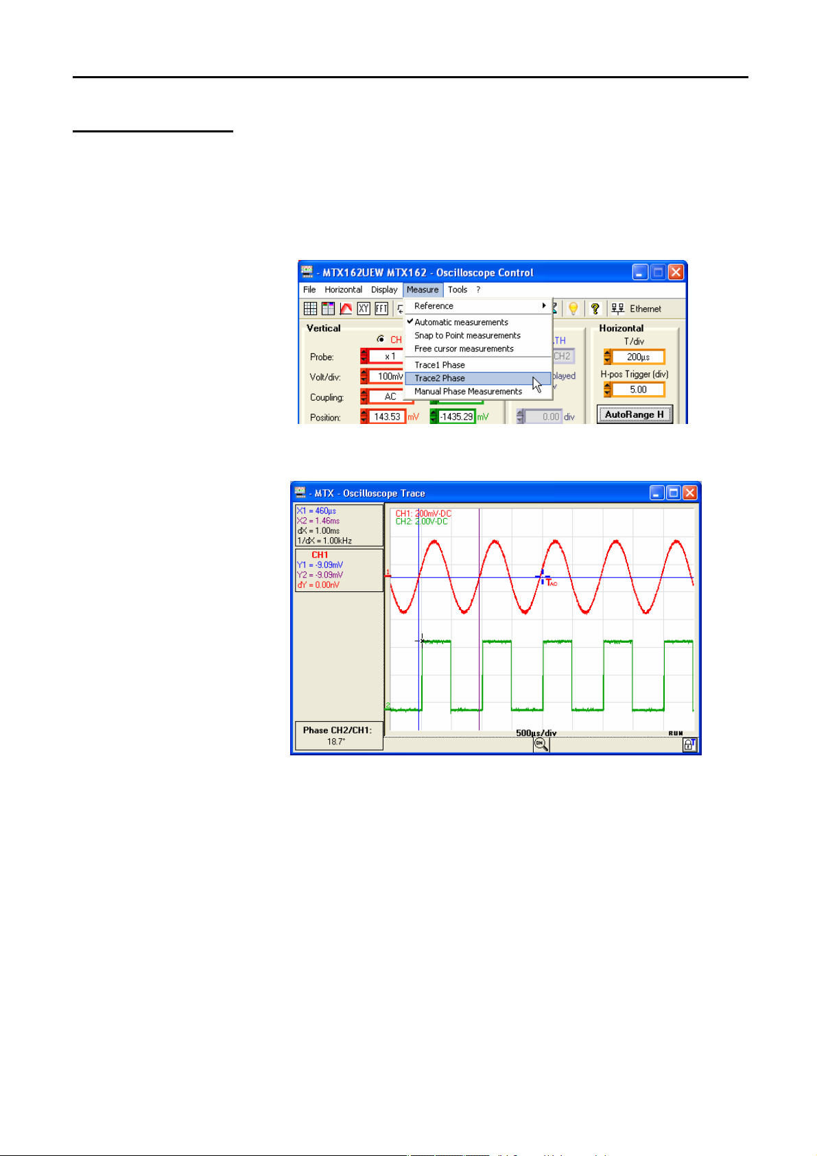
c) Manual phase

measurements

Cursors 1 & 2 are

placed on a period

of the reference

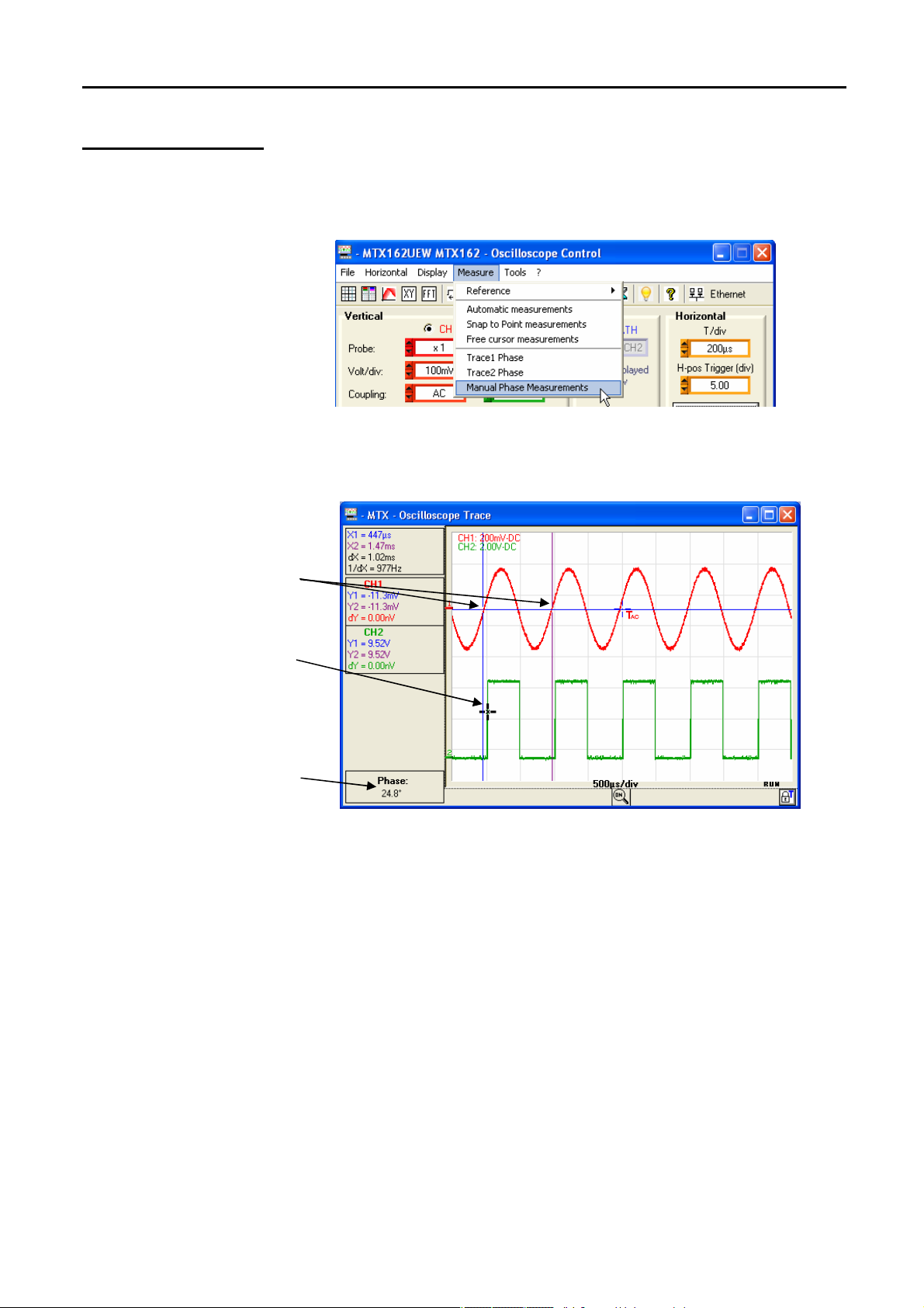
This function is used to measure the de-phasing between two signals. It is
completely manual and at the user's discretion.

It is activated from the 'Measure’ menu:

It shows a third cursor that must be placed on the other signal:

signal

The phase cursor

is placed on the

wave of the

secondary signal

Value of the CH2

phase compared

to CH1 in our

To measure a phase

example

The three cursors are free and can be placed anywhere in the trace display

ndow.

wi

• Place the cursors "1 = blue" and "2 = violet" on the "reference" signal to

determine its period for the phase calculation (this period corresponds to
360°).

• The "black" cursor is then placed on the other signal: if cursor 1 is

placed on an ascending wave with coordinates (X1,Y1), the black cursor
should be placed on the ascending wave of the other signal, as close to
X1 and on the same Y-Axis Y1 position as cursor 1.

The de-phasing value compared to the reference signal is given in
degrees.

 A de-phasing only has meaning if the two signals have the same

frequency.

Find Quality Products Online at: [e-mail]

VI - 32 Virtual digital oscilloscopes, 60 MHz

www.GlobalTestSupply.com

Making measurements from the trace

P

low

high

avg

L-

tm

td

Making measurements from the trace (continued)

2. Automatic measurements

a) General

measurements

on a channel

There are two types of automatic measurement: a) general measurements on a channel

b) automatic phase measurement

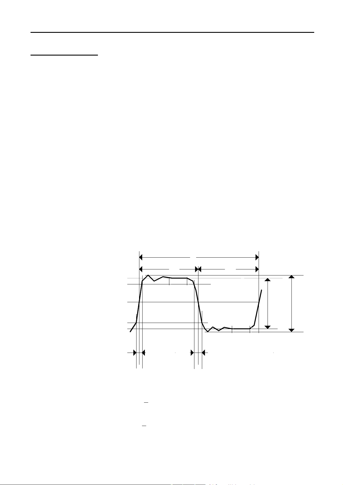
This function makes it possible to view the results of 19 automatic
measurements in a new window:

Vmin
Vmax
Vpp
Vlow
Vhigh
Vamp
Vrms
Vavg
Over+
Trise
Tfall
L+
L­P
F
DC
N
Over­Sum

minimum peak voltage
maximum peak voltage
peak to peak voltage
established low voltage
established high voltage
amplitude
operating voltage
average voltage
positive offset
ascending time
descending time
width of positive pulse (at 50% Vamp)
width of negative pulse (at 50% Vamp)
period
frequency
duty cycle ratio
number of pulses
negative offset

sum of elementary areas (= integral)

T = 1/F

W+ W-

L+

100%

90%

Vavg

>5%T

50%

10%

0%

Trise

• Positive offset = [100 * (Vmax – Vhigh)] / Vamp

• Negative offset = [100 * (Vmax – Vlow)] / Vamp

i n

=

1

• Vrms =

• Vavg

[ (y y ) ]

∑

n

i 0

=

n

=

i

1

=

(y y )

∑

n

=

i 0

Tfall

GND

GND

2 1/2

−

i

−

i

Vmax

Vhigh

Vamp Vpp

Vlow

Vmin

>5%T

Y

= value of the point representing zero Volts

GND

Find Quality Products Online at: [e-mail]

Virtual digital oscilloscopes, 60 MHz VI - 33

www.GlobalTestSupply.com

Making measurements from the trace

Making measurements from the trace (continued)

a) General

measurements

on a channel

(continued)

These measurements are made on the channel selected as reference
(see above).

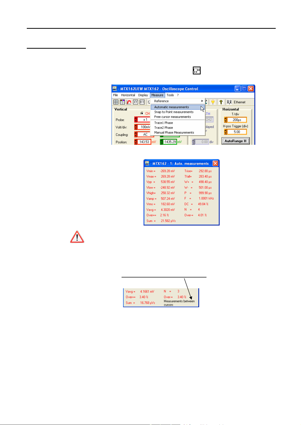
This function is activated: either using the button on the tool bar, or
from the 'Measurement’ menu:

It opens a new window called 'Auto measurements’:

By default the measurements are made on all the acquired points
(50 000 points) for the channel in question each time the
SCOPEin@BOX_LE application requests the transfer of curves.

However, if the manual cursors are active the measurements are
made using all the samples acquired in the interval determined by
cursors 1 & 2.
A message ‘Measurements between cursors

For a greater precision in the displayed measurements:

1. Represent at least two complete signal periods.

2. Prefer the "Triggered" acquisition mode rather
than "Automatic" (to avoid the artificial triggering related to this
mode with slow signals).

3. Choose the calibre and the vertical position in order to represent
the peak to peak amplitude of the signal to be measured on 4 to 7
divisions of the screen.

’ appears in the window:

4. If the signal allows (repetitive signal), the introduction of
acquisition averaging will refine the measurements by reducing
the noise effects on the measured signal.

Find Quality Products Online at: [e-mail]

VI - 34 Virtual digital oscilloscopes, 60 MHz

www.GlobalTestSupply.com

Making measurements from the trace

Making measurements from the trace (continued)

b) Automatic phase

measurement

When possible it determines the de-phasing of the CH1 or CH2 signal
compared to the reference channel (see above).

As with the manual phase measurement, 3 cursors are used, but they are
placed automatically.

This measurement is activated from the 'Measurement’ menu:

The "Oscilloscope Trace" window becomes:

Find Quality Products Online at: [e-mail]

Virtual digital oscilloscopes, 60 MHz VI - 35

www.GlobalTestSupply.com

Carrying out specific processes

Carrying out specific processes

1. Min/Max high resolution acquisition

2. Averaging the trace

In order not to hide the rapid voltage variations due to signal sub-sampling
for slower time bases the MTX 162 has a Min/Max high resolution
acquisition mode.

When this option is activated each pair of acquired points is the result of a
search for extreme min. and max. values from all the samples acquired
using the highest sampling speed, i.e. 50 MSamples/s.

This Min/Max acquisition mode guarantees that any peaks in voltage of
more than 40 ns width are seen and displayed on the oscilloscope screen.

This mode is activated from the 'Horizontal’ menu:

To reduce the random noise observed on the signals it is possible to
average the acquired samples.

The calculation is made using the following formula:

Pixel N = Sample*1/Averaging rate + Pixel

where: Sample Value of the new sample acquired at abscissa t

(1-1/Averaging rate)

N-1

Pixel N Y-Axis of the abscissa t pixel on the screen, at time N

Pixel N-1 Y-Axis of the abscissa t pixel on the screen, at time N-1

This averaging is activated using the 'Horizontal’ menu by selecting an
averaging rate different from: "No averaging".

When averaging is activated its rate is displayed in the "Oscilloscope
Trace" window:

In the case of a non repetitive signal do not activate
do not want an erroneous representation.

averaging if you

Find Quality Products Online at: [e-mail]

VII - 36 Virtual digital oscilloscopes, 60 MHz

www.GlobalTestSupply.com

Carrying out specific processes

Carrying out specific processes (continued)

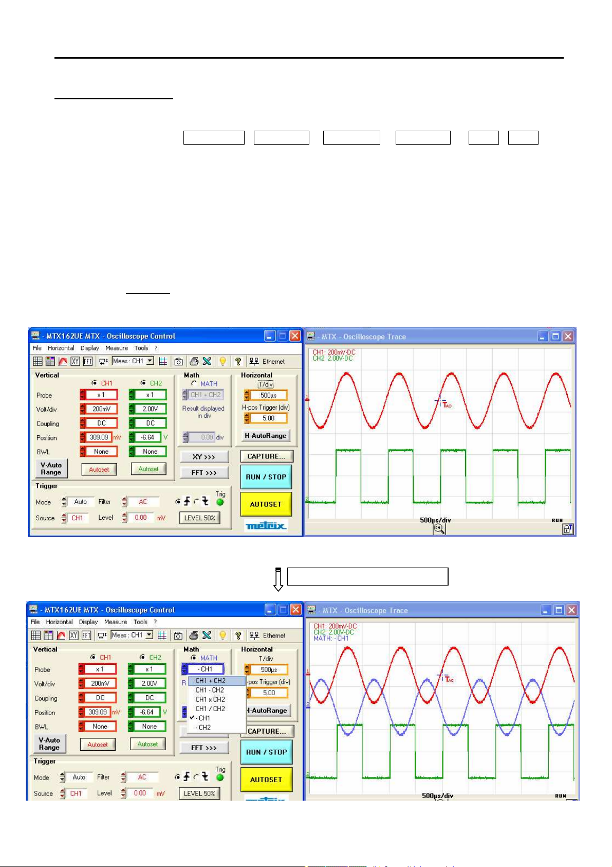
3. MATH trace

 Example

A third trace: MATH, is available on the MTX 162 to display one of the 6
proposed mathematical functions:
CH1 + CH2 CH1 - CH2 CH1 x CH2 CH1 / CH2 - CH1 - CH2

The vertical position of the MATH trace can be adjusted by ± 10 div.

 The mathematical functions are not calculated using the physical

size of the signals but using their base sample values converted
into divisions on the screen. This is why the vertical sensitivity of
the MATH channel is in div.

 To facilitate the analysis of the result it is recommended to work

ith the same calibration on both channels.

w

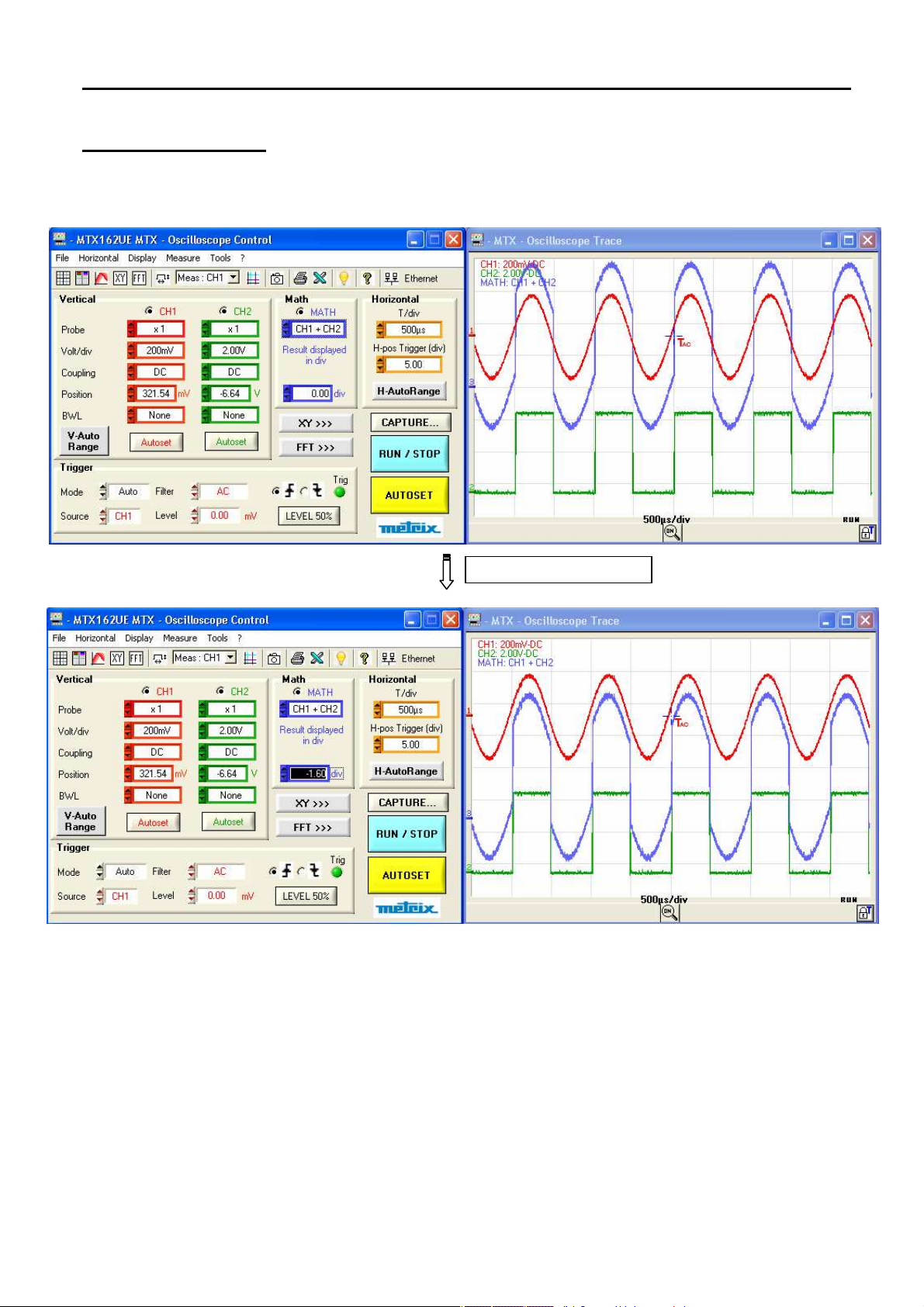
Insertion of the MATH function that adds signals CH1 and CH2.
An offset may be necessary to centre the trace on the screen.

Activation of the MATH block

Find Quality Products Online at: [e-mail]

Virtual digital oscilloscopes, 60 MHz VII - 37

www.GlobalTestSupply.com

Carrying out specific processes

Carrying out specific processes (continued)

3. MATH trace
(continued)

Offsetting the result

Find Quality Products Online at: [e-mail]

VII - 38 Virtual digital oscilloscopes, 60 MHz

www.GlobalTestSupply.com

Carrying out specific processes

Carrying out specific processes (continued)

4. Calculating an FFT

a) Launching the

FFT calculation

The Fourier signal transformation calculation is activated in 2 ways:

• by clicking on the button in the tool bar

• by clicking on the button in the "Control" panel:

In both cases a new "FFT Trace" window opens and a new FFT block is
added to the "Oscilloscope Control" panel programming this function:

Find Quality Products Online at: [e-mail]

Virtual digital oscilloscopes, 60 MHz VII - 39

www.GlobalTestSupply.com

Carrying out specific processes

Carrying out specific processes (continued)

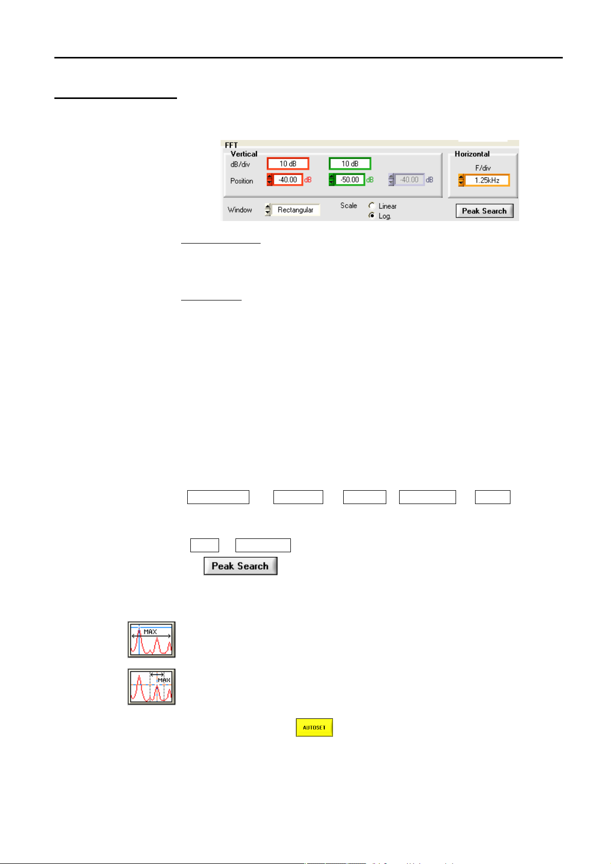
b) FFT settings

Vertical setting

Horizontal trace scale

The settings needed for this function are concentrated in the FFT block on
the "Oscilloscope Control" panel.

Logarithm scale:

- The vertical sensitivity of the FFT representation is of 10 dB/div.

- The 0 dB position corresponds to the top part of the screen.

The trace can be offset from +60 dB to -140 dB.

Linear scale:

- The vertical sensitivity of the FFT representation is that of the
channel.

- The 0V position places the channel reference in the 'Trace FFT'
window on the 1st division from the bottom of the screen.
The offset is adjustable from 0 to 8 div.

This sensitivity is directly related to the time base of the time representation
(unit Hz / div. : 12.5 / time base).
It varies from 62.5 mHz to 125 MHz.

Choice of the

calculation window

Choice of the

representation scale



Windowing makes it possible to limit to discontinuous effects related to the
time signal observation window (see §. Interpreting the FFT).

Five windows are available:

Rectangular Hamming Hanning Blackmann Flattop

Two FFT representation modes are possible:
linear or logarithmic

The button activates/deactivates the attached cursors to
make manual measurements on the FFT trace. It also leads to the display
or not of the buttons for automatic spectrum ray search.

positions cursor 1 on the maximum amplitude peak shown in the window.

places the active cursor on the maximum amplitude value found in a
window of ± 0.25 div. around this cursor. The search window is shown by a
black rectangle when pressing the key.

If an autoset is made when the FFT window is active the
automatic setting of the frequency scale will be made in order to place
the fundamental on approximately the first division.

A zoom may be needed on the time representation to correctly view
the signal.

Find Quality Products Online at: [e-mail]

VII - 40 Virtual digital oscilloscopes, 60 MHz

www.GlobalTestSupply.com

Carrying out specific processes

Carrying out specific processes (continued)

c) Interpreting

the FFT



The Fourier Fast Transformed (FFT) is used to calculate the discrete
representation of a signal in a frequency domain using its discrete
representation in the time domain.

FFT can be used for the following applications:

• measuring the different harmonics and the distortion of a signal,

• analysing an impulse response,

• searching for sources of noise in logical circuits.

The Fourier fast transform is calculated using the equation:

N

1

−

2

X (k) =

1 2

N

x n j

* ( ) * exp −

∑

N

n

=−

2





π

N

nk



for k ∈




∈ [0 (N – 1) ]

∈∈

where: x (n) : a sample in the time domain
X (k) : a sample in the frequency domain
N : FFT resolution
n : time index
k : frequency index

This calculation is made on 2500 points obtained by selected one
point every 20 in the acquisition memory.
These same points are used for the non zoomed time representation
in the "Oscilloscope Trace" window.

The finite duration of the studied interval is shown by a convolution in the
signal's frequency domain using a sinx/x function.
This convolution changes the FFT graphic representation because of the
lateral lobes that are characteristic of the sinx/x function (except if the study
interval contains a whole number of periods).

Before calculating the FFT, the oscilloscope weights the signal to be
analysed using a window that acts as a high-pass filter. The choice of a
type of window is essential to distinguish the different signal rays and make
precise measurements.

Time representation of the
signal to be analysed

Weighting window

Weighted signal

Frequency representation
of the signal calculated
using FFT

Find Quality Products Online at: [e-mail]

Virtual digital oscilloscopes, 60 MHz VII - 41

www.GlobalTestSupply.com

Carrying out specific processes

Carrying out specific processes (continued)

The following table can be used to select the type of window depending on
the type of signal, the desired spectrum resolution and the precision of the
amplitude measurement:

Window Type of signal

Rectangular transitory the best poor poor - 13 dB

Hamming random good correct correct - 42 dB

Hanning random good good correct - 32 dB

Blackmann

Flat Top sinusoidal poor good the best - 93 dB

random or
mixed

Frequency
resolution

poor the best good - 74 db

Spectrum
resolution

Amplitude
precision

Highest
lateral lobe

The following table gives the maximum theoretical error on the amplitude
for each type of window:

Window Max. theoretical

error
in dB

Rectangular 3,92

Hamming 1,75

Hanning 1,42

Blackmann 1,13

Flat Top < 0,01

This error is related to the FFT calculation when there is not a whole
number of periods in the observation window.

Thus, with a 'Flat Top' window, the 0 dB level is obtained on the ray of the
fundamental of a sinusoidal 1 Vrms amplitude signal.



Be careful to respect the Shannon theory, i.e. that the sampling
frequency "Sf" must be greater than 2 times the maximum frequency
containing by the signal.

If this condition is not respected spectrum folding phenomena are
observed.

Find Quality Products Online at: [e-mail]

VII - 42 Virtual digital oscilloscopes, 60 MHz

www.GlobalTestSupply.com

Carrying out specific processes

Zoom decrease

Horizontal scale

Left zoom

Carrying out specific processes (continued)

0 dB

origin

Reference

traces

d) Graphical

representation

Origin of the

frequency

The instrument simultaneously displays the FFT and the trace f(t).

The curve displayed in the 'FFT Trace’ window represents the amplitude in
V or dB for the different frequency components of the signal depending on
the selected scale.

The continuous component of the signal is removed by the software.

Two representations are possible:

Logarithmic representation

0V trace

origin

Origin of the frequency

Linear representation

Zoom

activation

When the zoom is activated only the zoomed zone is displayed:

of the zoomed trace

Horizontal

representation scale

Zoom

activation

scrolling button

Location of the

displayed zoomed

zone in the memory.

Exit zoom

Zoom increase

Right zoom scrolling

button

The displacement of the zoomed zone is done using the mouse by moving
the scroll bar or the scroll buttons.

Find Quality Products Online at: [e-mail]

Virtual digital oscilloscopes, 60 MHz VII - 43

www.GlobalTestSupply.com

Carrying out specific processes

Carrying out specific processes (continued)

d) Graphical

representation

(continued)





In order not to deform the spectral content of the signal and obtain a
better FFT calculation precision it is recommended to work with a
peak to peak amplitude of 3 div. to 7 div.

Too weak amplitude leads to a reduction in the precision and a too high
amplitude of over 8 divisions causes signal distortion, this causes
undesirable harmonics to appear.

The simultaneous time and frequency representation of the signal eases
the surveillance of the changes in signal amplitude.

Effects of under-sampling on the frequency representation:
If the sampling frequency is not adapted (less than double the maximum

frequency of the signal to be measured) high frequency components are
under sampled and appear on the FFT graphical representation by
symmetry (folding).

The "General Autoset" function avoids this phenomenon and adapts the

horizontal scale so that the representation is more legible.

e) Exit the FFT

calculation

There are three ways to exit the FFT representation:

• by clicking on the button in the tool bar

• by clicking on the button in the "Control" panel:

• by directly closing the 'FFT Trace' window:

Find Quality Products Online at: [e-mail]

VII - 44 Virtual digital oscilloscopes, 60 MHz

www.GlobalTestSupply.com

Carrying out specific processes

Carrying out specific processes (continued)

5. Obtaining an XY representation

a) Starting the XY

representation

The MTX 162 oscilloscope can be used to view the XY representation of
channels 1 and 2 in real time with X=CH1 and Y=CH2.

The XY representation is activated either:

• by clicking on the button in the tool bar,

• by clicking on the button in the "Control" panel:

In both cases a new XY window opens:

Find Quality Products Online at: [e-mail]

Virtual digital oscilloscopes, 60 MHz VII - 45

www.GlobalTestSupply.com

Carrying out specific processes

Carrying out specific processes (continued)

5. Obtaining an XY
representation
(continued)

b) Using the trace

The vertical calibrations of the traces selected for XY display can be
indicated at the top left of the window by clicking on the button of the

tool bar.

The measurements using cursors are available for the XY representation
and are used in the same way as in the "Oscilloscope trace" window
(see Chapter IV 

The manual measurement cursors for the "XY Trace" window are
independent of those in the "Oscilloscope Trace" window and are free
(not attached to the trace).

Manual Measurements using cursors).





Find Quality Products Online at: [e-mail]

VII - 46 Virtual digital oscilloscopes, 60 MHz

www.GlobalTestSupply.com

Carrying out specific processes

Carrying out specific processes (continued)

5. Obtaining an XY
representation
(continued)

c) Cancelling the XY

representation

There are three ways to exit the XY representation:

• by clicking on the button in the tool bar

• by clicking on the button in the "Control" panel:

• by directly closing the 'XY Trace' window:

Find Quality Products Online at: [e-mail]

Virtual digital oscilloscopes, 60 MHz VII - 47

www.GlobalTestSupply.com

Carrying out specific processes

Carrying out specific processes (continued)

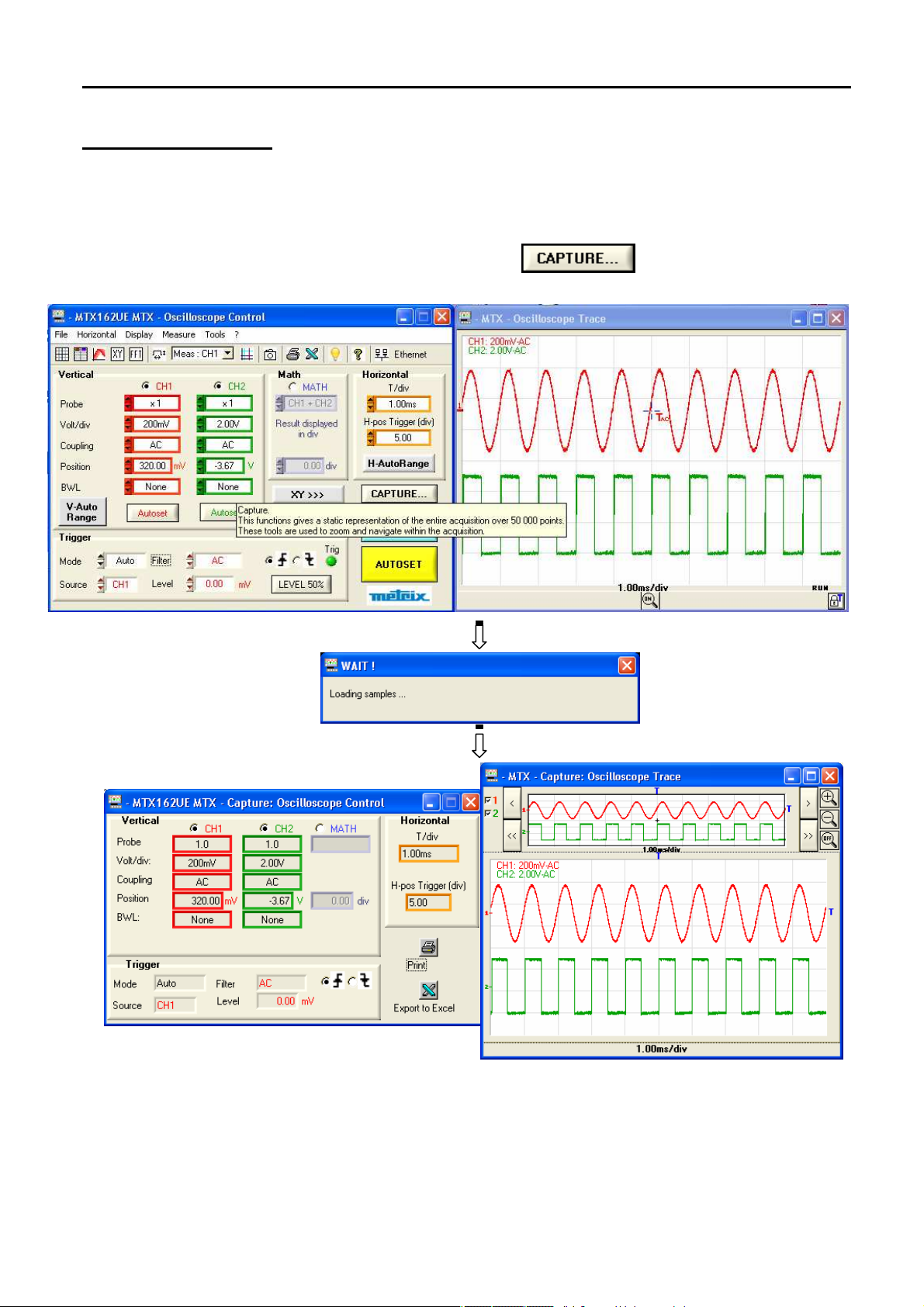
6. Capturing traces

a) Starting the

capture

Capture is used to recall complete traces (50 000 samples per channel) to
the PC in order to analyse the signal at a given moment while continuing to
view it in real time in the "Oscilloscope Trace" window.
During capture the acquisition is stopped while the points are transferred.

The capture is started using the key in the
"Oscilloscope Control" window:

The "Capture: Oscilloscope Control" window summarises the settings used
to make these acquisitions.

The "Capture: Oscilloscope Trace" window contains the representation of
the acquired points.

Find Quality Products Online at: [e-mail]

VII - 48 Virtual digital oscilloscopes, 60 MHz

www.GlobalTestSupply.com

Carrying out specific processes

Carrying out specific processes (continued)

6. Capturing traces (cont.)

b) Using the data

Graph of the entire

acquisition memory

Selection of

the channel display

Offset 1 div.

zoomed to the left

Offset 8 div.

zoomed to the left

Display of vertical scales

(if active)

Graph of the zoomed

zone

Marking of the

zoomed zone

Horizontal trigger
position

Offset 1 div. zoomed to
the right

Zoom increase

Zoom decrease

Exit zoom

Offset 8 div zoomed.
to the right

Acquisition time
base

Horizontal trigger
position

Zoomed horizontal
scale

The measurements using cursors are available for the C

apture and are

managed in the same way as in the "Oscilloscope trace" window
(see Chapter IV 

 Cursors):



Trigger
level



Phase measurement is not available in capture.

Find Quality Products Online at: [e-mail]

www.GlobalTestSupply.com

Virtual digital oscilloscopes, 60 MHz VII - 49

Carrying out specific processes

Carrying out specific processes (continued)

6. Capturing traces
(continued)

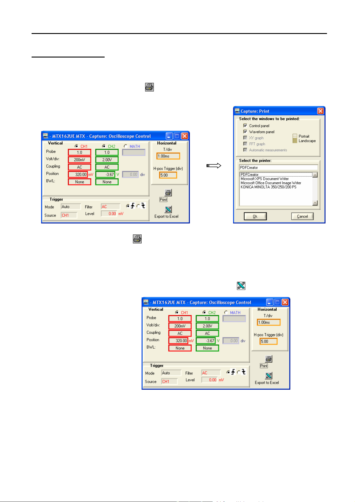
c) Printing the

capture

Pressing the key starts printing the "Capture" windows from the
"Capture : Oscilloscope Control" panel:

 The button on the tool bar of the "Oscilloscope Control

window or the File 
captures.

d) Exporting the

ture to EXCEL

cap

Current captures can be exported to EXCEL from the "Capture :
Oscilloscope Control" panel by pressing the button:

The "Export to EXCEL..." window opens (see §. Chapter X).

 Print menu do not allow the printing of



Find Quality Products Online at: [e-mail]

VII - 50 Virtual digital oscilloscopes, 60 MHz

www.GlobalTestSupply.com

Carrying out specific processes

MEM2

Zoomed time base for MEM2

Carrying out specific processes (continued)

6. Capturing traces
(continued)

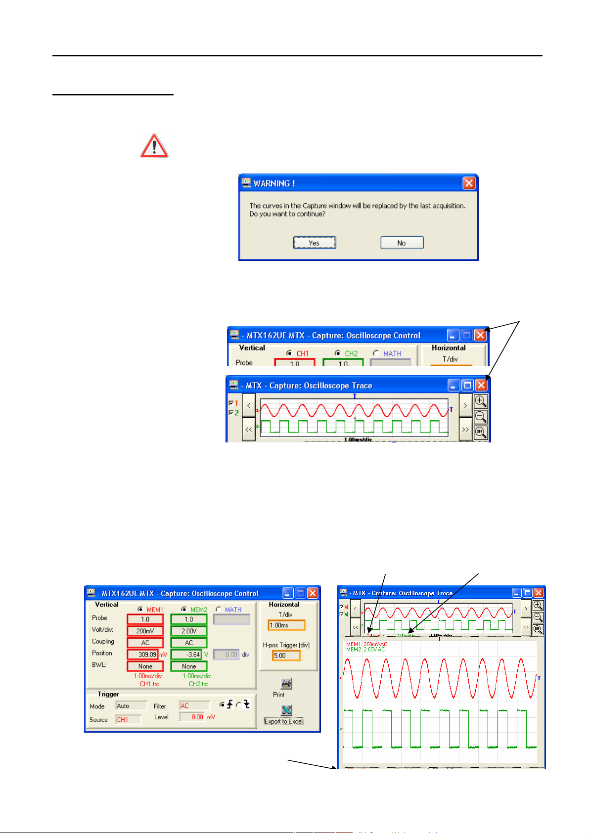
e) Cancelling trace

capture

Exporting to EXCEL from the "Oscilloscope Control" panel causes a
new capture and therefore the loss of the current capture. The
following message appears:

If you wish to export the current captures click on 'No'.

To exit close one of the "Capture" windows:

or



The closure of the 'Capture' windows leads to the permanent loss of
the traces.
If you wish to keep the captured traces to work on them further stop
acquisition, make a backup of the signals in question in a ".TRC" file
just after having carried out the capture.
All that needs to be done then is to recall these traces and make a
new capture with these MEMx traces (see §. Recalling the trace).

Acquisition time base for

MEM1

Acquisition time base for

Zoomed time base for MEM1

Find Quality Products Online at: [e-mail]

Virtual digital oscilloscopes, 60 MHz VII - 51

www.GlobalTestSupply.com

Freezing, Saving, Displaying the trace

CH1 and CH2

Freezing, Saving, Displaying the trace

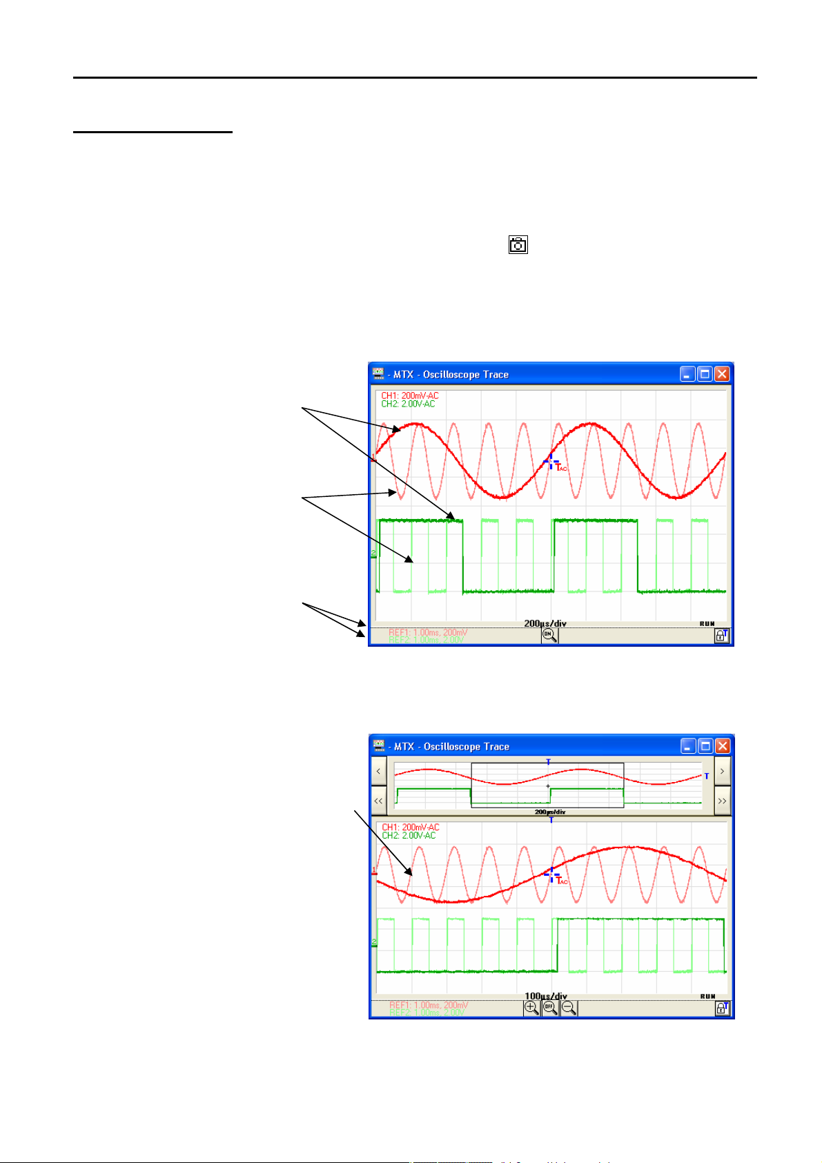
1. Freezing the trace

Traces of channels

Frozen traces of

channels CH1 and CH2

To highlight an eventual signal variation it is possible to freeze the traces at
a point in time. These traces appear in a light colour in the 'Oscilloscope
Trace' window.

A trace can only be frozen if it is on the screen.

This trace "snapshot" is made using the button on the tool bar. Pressing
the button again erases the current frozen traces.

 The frozen trace is not lost if you exit and open new work session

using the same instrument configuration file

Sensitivity and

acquisition time base

for the frozen traces

De-selecting a channel permanently deletes its snapsho

These frozen traces are static display data: activating the zoom therefore
has no effect on them and they cannot be moved up or down.

For a zoom the

frozen traces

only appear on

the zoomed

graph.

t.

Find Quality Products Online at: [e-mail]

VIII - 52 Virtual digital oscilloscopes, 60 MHz

www.GlobalTestSupply.com

Freezing, Memorizing, Displaying the trace

Freezing, Memorizing, Displaying the trace (continued)

2. Saving the trace

a) ".TRC" saving



Example

The MTX 162 gives the possibility of saving the traces displayed on the
screen.

Two memorization formats are available: ".TRC" or ".TXT".

In both cases the 50 000 acquired samples that form the trace as well as the
data relating to the acquisition and making it possible to interpret the data
are transferred to the PC are backed up.

This is the only format that can be used to reload a trace into the
oscilloscope (see §. Recalling the trace). It is a binary file with a ".TRC"
extension that can only be used by the SCOPEin@BOX_LE software.

Saving CH1 trace in the 'Trace1.trc' file

Find Quality Products Online at: [e-mail]

Virtual digital oscilloscopes, 60 MHz VIII - 53

www.GlobalTestSupply.com

Freezing, Saving, Displaying the trace

the trace

Freezing, Memorizing, Displaying the trace (continued)

2. Saving
(continued)

b) ".TXT"saving



Example

This format is used to export data to another application (spreadsheet,
editor…).

However the generated file cannot be used by SCOPEin@BOX_LE.

It is a test file (ASCII) with the ".TXT" extension that can be viewed using
any editor programme.

Saving CH1 trace in the 'Trace1.txt' file

Find Quality Products Online at: [e-mail]

VIII - 54 Virtual digital oscilloscopes, 60 MHz

www.GlobalTestSupply.com

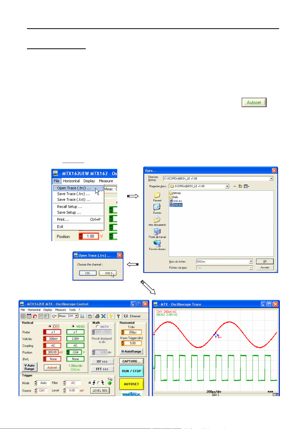
Freezing, Memorizing, Displaying the trace

Freezing, Memorizing, Displaying the trace (continued)

3. Recalling the

trace

 Example

Only the trace files backed up using SCOPEin@BOX_LE and having the
".TRC" extension can be recalled by the application.

These traces can replace either the CH1 and/or the CH2 traces.

In the 'Oscilloscope Control' window the channel name is displayed as
MEMx, and the settings for the vertical block for the channel in question are
updated using the values contained in the file. The acquisition time base of
the recalled trace and the file name are displayed instead of .

The deletion of the recall is made by de-selecting the MEMx channel which
returns to CHx.

The recalled trace behaves in the same way as a normal trace: they



can moved up or down and all the available automatic or manual
measurements can be carried out.

Recall of the 'Trace1.trc' file on the CH2 channel

Find Quality Products Online at: [e-mail]

Virtual digital oscilloscopes, 60 MHz VIII - 55

www.GlobalTestSupply.com

*

Memorizing, Recalling the configuration

Memorizing, Recalling the configuration

The general instrument configuration is the set of data that makes
it possible to restart the device in the same status as it was in
when the last session was closed.

An automatic backup of the general configuration is made every
time a session is closed.

This general configuration is stored at the same level as the
"SCOPEin@BOX_LE.exe" executable on the PC's hard drive.

It has three files:

setup.7up

This is the configuration file for the SCOPEin@BOX_LE software;
it contains the following data:

- first install indicator

- language used

- software work directory

<nameInstrument>.INI

where <nameInstrument> is the name given to the instrument
when a session is created.

<nameInstrument>.INI.CFG

The ".INI" file is the PC configuration, it includes the following
data:

- the size and location of all the open windows

- the access paths to the various directories (trace
backups, configurations, software updates...)

- identification of the software and equipment versions

- information relative to the instrument being used
(oscilloscope name, serial number, MAC address, IP

dress …)

ad

- the previously used communication mode
(Ethernet/USB)

- trace references

- etc. …

The ".CFG" file is the oscilloscope configuration, it contains all the
current instrument settings.

Find Quality Products Online at: [e-mail]

IX - 56 Virtual digital oscilloscopes, 60 MHz

www.GlobalTestSupply.com

Memorizing, Recalling the configuration

Memorizing, Recalling the configuration (continued)

1. Memorizing the configuration



Example

This backup only covers the oscilloscope configuration, the PC configuration
is specific to the open session.

During the backup the oscilloscope configuration is stored in a file with a
".CFG" extension which it is recommended to place in a specific directory in
order to differentiate it from general configurations (in the example below we
have created a CFG directory).

The access path to this directory is memorized in the PC configuration so
that the user will be directed to this directory by default for all operations
pertaining to configuration management.

Backup of the oscilloscope configuration in config1.cfg.

Find Quality Products Online at: [e-mail]

Virtual digital oscilloscopes, 60 MHz IX - 57

www.GlobalTestSupply.com

Memorizing, Recalling the configuration

Memorizing, Recalling the configuration (continued)

2. Recalling the configuration



Example

Only configurations made using the SCOPEin@BOX_LE application can be
recalled, configurations for oscilloscopes other than MTX 162 are not
compatible.

Recall of the "config1.cfg" configuration

Find Quality Products Online at: [e-mail]

IX - 58 Virtual digital oscilloscopes, 60 MHz

www.GlobalTestSupply.com

Exporting the trace to EXCEL

Exporting the trace to EXCEL

To export the trace the PC must first recall the 50 000 samples acquired from
the oscilloscope; this is why the Capture windows open if they are not already
open.

The samples can be transferred to EXCEL in three ways:

• by clicking on the button in the tool bar,

• from the 'Tools/Export to EXCEL…' menu

• from the "Capture: Oscilloscope Control" window by pressing the

button:

Find Quality Products Online at: [e-mail]

Virtual digital oscilloscopes, 60 MHz X - 59

www.GlobalTestSupply.com

Exporting the trace to EXCEL (continued)

Exporting the trace to EXCEL

The following window appears:

Find Quality Products Online at: [e-mail]

X - 60 Virtual digital oscilloscopes, 60 MHz

www.GlobalTestSupply.com

Exporting the trace to EXCEL

Exporting the trace to EXCEL (continued)



The export of data to Excel can take several minutes.

This export can be done manually using the trace saving (.TXT) which is
opened directly using EXCEL (see §. Using 

 Save.TXT).



Find Quality Products Online at: [e-mail]

Virtual digital oscilloscopes, 60 MHz X - 61

www.GlobalTestSupply.com

Technical specifications

Technical specifications

Vertical offset

Characteristics Specifications Observations

Number of channels

Types of entry

Bandwidth to - 3 dB

Dynamics of vertical offset

Entry Coupling

Bandwidth Limit

Rise time

Cross-talk between channels

Only the assigned tolerance or limit values are guaranteed (after
30 minutes to adapt to temperature).
Values without tolerances are given for information purposes only.

2 channels: CH1 - CH2 BNC entries

Class 1, common masses

≥ 60 MHz on all vertical ranges

from 5 mV to 5 V/div.

≥ 20 MHz on ranges 10 V/div. to

100 V/div. ( the bandwidth limitation
for these calibres is related to the
HF power limitation in the entry
capacity attenuation network)

± 10 div. on all the ranges

AC, DC, GND

at 15 MHz, 1.5 MHz and 5 kHz one bandwidth limit per channel

≤ 5 ns (60 MHz) on vertical ranges

from 5 mV to 5 V/div.

DC at 50 MHz ≥ 40 dB

Measured on a charge of 50 Ω

with a 6 div. amplitude signal

depending on the model

same sensitivity on both channels

Tolerance ESD

Response to rectangular 1 kHz
and 1 MHz signals

Accuracy of vertical ranges

Vertical resolution

Accuracy of vertical
measurements

Accuracy of vertical offset

Probes

Vertical ZOOM function on an
acquire or backed up curve

maximum entry Voltage 400 Vpk (DC + peak AC at 1 kHz)

Electrical safety

± 2 kV

Overshoot < 3 %
Aberrations < 3 %

± 2 % (on a 6 div. amplitude signal)

± 0.4 % of the full scale
± [2 % (reading - offset)

+ Precision of vertical offset
+ (0.05 div.) x (volt/div.)]

± [0.01 x (offset value)

+ 4 mV + (0.1 div.) x (V/div.)]

Attenuation coefficients of the probe
and its graphical representation are
taken into account in the display

no vertical Zoom

without the sensors

300 V, CAT II without sensors

Positive or negative overshoot

Sequence of vertical ranges
1 - 2 - 5

Variation in bounds (no continuous
variable rate)

Entry Impedance

Display modes

Find Quality Products Online at: [e-mail]

XI - 62 Virtual digital oscilloscopes, 60 MHz

1 Mohm ± 1 % 13 pF ± 2 pF

"Multi-window" with the possibility of
displaying the f(t) trace, the FFT
and the XY mode simultaneously

www.GlobalTestSupply.com

Default display: control window +
trace window
Double time base type display,
even in real time

Technical specifications

Technical specifications (continued)

Time base

Characteristics Specifications Observations

Ranges

Precision

Sampling frequency

Precision of time measurements

Display

Horizontal expansion

Triggering circuit

32 ranges, from 5 ns to 100 s/div. Sequence 1 - 2 - 5

Real time up to 2 µs/div.
(if 50 Msps acquisition and
1000 pts on the screen)

± 0.5 %

50 MS/s on all single acquisition
channels

± [(0.04 div.) x (time/div.)

+ 0.005 x (reading) + 1 ns]

Display of 1000 points on the screen

Simultaneous display of the 50 kpts
on 2500 points and the 2500 points
for the zoomed zone

Possibility of offsetting the zoomed
zone within the memory

20 GS/s in ETS mode

Max expansion x 20

Characteristics

Triggering sources

Triggering mode

Trigger coupling

Triggering slope

Trigger sensitivity in normal
mode

Source channels CHx

Noise Reject

Triggering level

Variation Range

Specifications Observations

Sources CH1, CH2, LINE

AUTO - NORMAL - SINGLE

DC : BP 0 to 100 MHz

AC : BP 10 Hz to 100 MHz

Descending wave or

Ascending wave

0.5 div

1.5 div

± 8 div.

Find Quality Products Online at: [e-mail]

Virtual digital oscilloscopes, 60 MHz XI - 63

www.GlobalTestSupply.com

Technical specifications

Technical specifications (continued)

Acquisition chain

Characteristics Specifications Observations

Resolution of the ADC

Max. sampling frequency

Sampling modes:

Real Time

Equivalent ETS Time

Transitory capture

Minimum width for detectable
glitches

Depth of acquisition memory

PRETRIG Function

CHx channel backup memories

Storage formats

8 bits

50 MS/s

50 MS/s max

Precision ± 200 ppm

20 GS/s max

> 20 ns

50 kpoints

Position of the trigger point using the
mouse

up to minimum 1500 traces
depending on the available PC
memory

"Trace

"TXT

"Config

1 8 bit converter per channel

Single non repetitive signals

Repetitive signals

Glitch capture can be activated for
all the time base ranges.

These files can be named and have
extensions.

Backup of the curve and the
acquisition settings

Backup of the complete
configuration

Find Quality Products Online at: [e-mail]

XI - 64 Virtual digital oscilloscopes, 60 MHz

www.GlobalTestSupply.com

Technical specifications

Technical specifications (continued)

Display

Characteristics Specifications Observations

Viewing Screen

Number of displayed points

Viewed in normal mode Window

ZoomH

Display modes

Average

Graticle

Indications in the
"Oscilloscope Trace" window

PC screen

2500 acquired points

Horizontal zoom: x 20

1 kpts (representing the Min/Max of the
acquired 50 kpts)

Horizontal expansion by: 50

Interpolation

Persistent display managed by the PC
display for the last 8 acquired traces using
8 tints of the color of the channel 
brightest color represents the most
recent acquisition and the dullest the
oldest

Envelope Mode

Factors: 2, 4, 8 ,16

Complete Axes Borders

 the



no vertical Zoom

Automatic measurements are
available in this mode: they are
made on the last acquired trace

Indicate that averaging is
activated on the trace window

triggering

Traces

Indications in the "Oscilloscope
Control" window

Predefined Mathematical
functions

Position of the T level (trace color) on the
left edge of the display window Horizontal
position of the Trig point on the top edge
of the window.

"Identifier + Mass reference" of the trace
color

"BWL » Band Width Limit:
High and low overshoot indicators if the
traces are outside the screen and right left
if the T position of the trigger point is not
on the screen

Menu bar:
Vertical, Horizontal, Display,
Measurement, Memory, Utilities, Help

Active mathematical calculations:
FFT, ADD, SUBS, MULT, DIV, INVersion

Synthesis of the device configuration:
Vertical position and sensitivity
Time base range
Trigger mode
Trigger source

Find Quality Products Online at: [e-mail]

Virtual digital oscilloscopes, 60 MHz XI - 65

www.GlobalTestSupply.com

Technical specifications

Technical specifications (continued)

Mathematical functions

Other

Calibration Signal

Autoset

Search time

Frequency range

Amplitude range

Duty cycle

Communication interfaces

USB type B connector

Equation editor
Addition, subtraction, multiplication, division and complex functions

between channels

Form
Amplitude
Frequency

< 5 s
30 Hz to 60 MHz
40 mVpp to 400 Vpp
from 20 to 80 %

used to connect the scope to the PC using a USB cable.

Location on the back face of the oscilloscope
Interface "USB to RS232", the serial connection configuration

is automatic at 921 600 bauds, HARD protocol,
8 bits, 1 stop bit, no parity.

Driver The "USB to RS232" interface driver loads
automatically when the SCOPEin@BOX_LE software
is installed

Rectangular
0 - 2.5 V ± 2 %
1 kHz ± 1 %

ETHERNET Interface

Ethernet WiFi

Output power 14 + 2 / -1.5 dBm

Data speed 11 Mbps

Modulation DSSS, DBPSK, DQPSK, CCK, OFDM, 16QAM,

Security WEP 64/128, WPA, WPA2/802.11i

Max. reception

Receiver

Location on the back face of the device
Type 10BASE-T (Twisted Pair)
Connector RJ 45 8 points
Standard IEEE 802.3

Category

Frequency

range

level

sensitivity

IEEE 802.11b/g

2,400 - 2,484 GHz

64QAM

-10 dBm (with PER < 8 %)

- 88 dBm

Find Quality Products Online at: [e-mail]

XI - 66 Virtual digital oscilloscopes, 60 MHz

www.GlobalTestSupply.com

Technical specifications

Technical specifications (continued)

Programming the oscilloscope remotely from a PC

The oscilloscope can be programmed remotely using a PC using simple
standardised commands by using:

- the "USB to RS232" interface MTX 162UE

- ETHERNET interface (port 23) MTX 162UEW

The programming instructions comply with the IEEE 488.2 SCPI protocol
standard.

Refer to the remote programming instructions for the complete list of



commands and syntax rules.

Warning !

Error messages

Autotest : Error n°0001: Microprocessor or FLASH pr oblem
Autotest : Error n°0002: RAM problem
Autotest : Error n°0004: FPGA problem
Autotest : Error n°0008: SSRAM problem
Autotest : Error n°0010: SCALING 1 problem
Autotest : Error n°0020: SCALING 2 problem
Autotest : Error n°0040:
Autotest : Error n°0080:
Autotest : Error n°0100: channel 1 acquisition prob lem
Autotest : Error n°0200: channel 2 acquisition prob lem
Autotest : Error n°0400:
Autotest : Error n°0800:
Autotest : Error n°1000: Ethernet problem
Autotest : Error n°2000: Vernier problem

If one of these codes (or the sum of several codes) are shown when the
device is started up 

 a fault has been detected.



Find Quality Products Online at: [e-mail]

Virtual digital oscilloscopes, 60 MHz XI - 67

www.GlobalTestSupply.com

General specifications

General specifications

Environment

Power supply

Safety

CEM

• Reference temperature 18°C to 28°C

• Operating temperature 0°C to 40°C

• Storage temperature - 20°C to + 60°C

• Indoor use

• Altitude < 2000 m

• Relative humidity < 80 % up to 31°C

• Network voltage nominal usage range 100 to 240 VAC

• Frequency from 47 to 63 Hz

• Consumption < 14 W at 230 VAC - 50 Hz

• Fuse 2.5 A / 230 V / timed

• Power supply cable removable

Compliance IEC 61010-1 (2001):

• Insulation class 1

• Pollution degree 2

• Power supply surge category: CAT II 240 V

• "Measurement" entry power supply surge category: CAT II 300 V

This appliance was designed in compliance with the current CEM
standards and was tested in compliance with the NF EN 61326-1, 2006
standard: Immunity Influence: 5 mV in the presence of an electromagnetic
field of 10 V/m

European directives

This product is compliant with the European low voltage directives
2006/95/EC and the CEM 2004/08/EC European directive.

Mechanical specifications

Box

Packaging

• Size 270 x 213 x 63 (in mm)

• Weight 1.8 kg

• Materials ABS VO (auto extinguishing)

• Water tightness IP 30

• Size 300 (l) x 330 (L) x 230 () in mm

Find Quality Products Online at: [e-mail]

XII - 68 Virtual digital oscilloscopes, 60 MHz

www.GlobalTestSupply.com

Supply

Supply

Accessories

delivered

as options

• Operating instructions on CD ROM

• Programming instructions on CD ROM

• "SCOPEin@BOX_LE" software on CD ROM

• Getting started guide for the software on CD ROM

• Safety instructions

• Power supply cable

• Voltage sensors 1/1, 1/10, 100 MHz, 300 V (x 2)

• STRAIGHT-THRU Ethernet network cable

• Crossover Ethernet network cable

• USB cable

• T junction

1 x BNC male - 2 x BNC female (pack of 3 parts) HA2004-Z

• Female BNC - BNC female extension (pack of 3) HA2005

• Safety adapter

BNC male / 4 mm cartridge, CAT III, 500 V (pack of 3) HA2002

• Safety adapter

BNC male / 4 mm cartridge, CAT III, 500 V (pack of 2) HA2053

• Voltage sensors 1/1, 1/10, 200 MHz, 300 V HX0220

• Voltage sensor 1/10 fixed, 150 MHz, CAT II / 400 V HX0003

• Voltage sensor 1/10 fixed, 450 MHz, CAT II / 1,000 V HX0005

• Voltage sensor 1/100 fixed, 300 MHz, 5 kV Peak HX0006

• Differential sensor 1 channel 30 MHz MX9030-Z

• Differential sensor 2 channels 50 MHz BNC entries MTX1032-C

• Differential sensor 2 channels 30 MHz banana entries MTX1032-B

• BNC male / BNC male cable CAT III, 500 V, length 1 m AG1044

• Fuse 2.5 A, 230 V, timed, 5 x 20 mm AT0090

Find Quality Products Online at: [e-mail]

Virtual digital oscilloscopes, 60 MHz XIII - 69

www.GlobalTestSupply.com