Zurich Instruments HF2 User Manual

Download

Page 1

HF2 User Manual LabOne Edition

Page 2

HF2 User Manual - LabOne Edition

Zurich Instruments AG

The contents of this document are provided by Zurich Instruments AG (ZI), “as is”. ZI makes no representations or warranties with respect to the accuracy or completeness of the contents of this publication and reserves the right to make changes to specifications and product descriptions at any time without notice.

LabVIEW is a registered trademark of National Instruments Inc. All other trademarks are the property of their respective owners.

Revision History

Revision 34390, 22-Dec-2015:

This is the first version of the HF2 User Manual (LabOne Edition). The document is related to the 15.11 LabOne release.

Highlights of the changes and additions to the HF2LI product are:

• New Option HF2LI-WEB: LabOne control software is now available for all HF2 series instruments

• Sweeper: faster sweeps due to improved instrument communication

• Modulation: change in FM generation method improves spectral purity. Limited to narrow-band FM

signals

The HF2LI-WEB LabOne Web Interface comes with several new software tools that replace or extend the tools available in the Zurich Instruments ziControl software:

• PID: Tune function replaced by PID Advisor with extended DUT model library

• SW Trigger: scope-like data capture of streamed data, unavailable in ziControl

• Sweeper: LabOne Sweeper Reference replaces ziControl Sweeper Calibration and Reference

• Sweeper: new sweep parameters available in LabOne Sweeper: modulation amplitude and index

• Sweeper: advanced and application mode: configuration assistant for settling time/inaccuracy and

omega suppression

• Sweeper: Q-factor extraction unavailable in LabOne Sweeper

• Spectrum: LabOne Spectrum tab replaces ziControl zoomFFT tool

• Spectrum: modes FFT(Theta), FFT(f), FFT(dTheta/dt) unavailable in ziControl

• Spectrum: noise power analysis unavailable in LabOne Spectrum tab

• Plotter: LabOne Plotter replaces ziControl Spectroscope. Larger selection of plotted data, support for

multiple curves, more powerful plotting and analysis tools

Page 3

Declaration of Conformity ..................................................................................................... V

1. Getting Started ................................................................................................................. 6

1.1. Quick Start Guide ................................................................................................... 7

1.2. Inspect the Package Contents ................................................................................ 8

1.3. Software Installation ............................................................................................ 10

1.4. Handling and Safety Instructions .......................................................................... 16

1.5. Connecting to the Instrument ............................................................................... 18

1.6. Troubleshooting ................................................................................................... 28

2. Functional Overview ........................................................................................................ 32

2.1. Features .............................................................................................................. 33

2.2. Front Panel Tour .................................................................................................. 36

2.3. Back Panel Tour ................................................................................................... 38

2.4. Ordering Guide ..................................................................................................... 39

2.5. Operating Modes .................................................................................................. 41

3. Tutorials ......................................................................................................................... 46

3.1. Tutorial HF2LI First Time User .............................................................................. 47

3.2. Tutorial Simple Loop ............................................................................................ 54

3.3. Tutorial Dynamic Signals ...................................................................................... 58

3.4. Tutorial External Reference .................................................................................. 63

3.5. Tutorial Noise Measurement ................................................................................. 67

3.6. Tutorial Amplitude Modulation .............................................................................. 68

3.7. Tutorial Frequency Modulation ............................................................................. 72

3.8. Tutorial Phase-locked Loop .................................................................................. 76

4. Functional Description LabOne User Interface ................................................................. 80

4.1. User Interface Overview ........................................................................................ 81

4.2. Lock-in Tab .......................................................................................................... 92

4.3. Lock-in Tab (HF2-MF option) .............................................................................. 101

4.4. Numeric Tab ...................................................................................................... 110

4.5. Plotter Tab ......................................................................................................... 112

4.6. Scope Tab .......................................................................................................... 114

4.7. Software Trigger Tab .......................................................................................... 119

4.8. Spectrum Analyzer Tab ....................................................................................... 124

4.9. Sweeper Tab ...................................................................................................... 128

4.10. Auxiliary Tab .................................................................................................... 136

4.11. Inputs/Outputs Tab .......................................................................................... 138

4.12. DIO Tab ............................................................................................................ 140

4.13. Config Tab ........................................................................................................ 142

4.14. Device Tab ....................................................................................................... 146

4.15. File Manager Tab .............................................................................................. 148

4.16. PLL Tab ............................................................................................................ 150

4.17. PID Tab ............................................................................................................ 156

4.18. MOD Tab .......................................................................................................... 165

4.19. Real-time Tab .................................................................................................. 170

4.20. HF2CA Tab ....................................................................................................... 171

4.21. HF2TA Tab ....................................................................................................... 173

4.22. ZI Labs Tab ...................................................................................................... 175

5. Communication and Connectivity ................................................................................... 176

5.1. Instrument Connectivity Overview ....................................................................... 177

5.2. ziServer's Text-based Interface ........................................................................... 182

5.3. Connecting to ziServer over insecure or firewalled networks ................................. 191

6. Node Definitions ........................................................................................................... 194

6.1. Overview ............................................................................................................ 195

6.2. Nodes ................................................................................................................ 205

7. Real-time Option ........................................................................................................... 281

HF2 User Manual - LabOne Edition Revision 34390 Zurich Instruments 3

Page 4

7.1. Installation of the Real-time Development Environment ....................................... 282

7.2. Real-Time Option Reference Manual ................................................................... 286

8. Specifications ............................................................................................................... 609

8.1. General Specifications ........................................................................................ 610

8.2. Analog Interface Specifications ........................................................................... 612

8.3. Digital Interface Specifications ........................................................................... 616

8.4. Performance Diagrams ....................................................................................... 619

8.5. Ground and Earth Scheme .................................................................................. 629

8.6. Reference Images ............................................................................................... 631

8.7. Test Specifications ............................................................................................. 635

9. Signal Processing Basics ............................................................................................... 636

9.1. Principles of Lock-in Detection ........................................................................... 637

9.2. Signal Bandwidth ............................................................................................... 640

9.3. Discrete-Time Filters .......................................................................................... 642

9.4. Full Range Sensitivity ......................................................................................... 644

9.5. Sinc Filtering ...................................................................................................... 646

9.6. Zoom FFT ........................................................................................................... 649

10. HF2CA Current Amplifier Data Sheet ............................................................................ 651

10.1. Key Features .................................................................................................... 652

10.2. Specifications .................................................................................................. 653

10.3. Functional Description ...................................................................................... 656

10.4. Applications ..................................................................................................... 658

10.5. Cable Recommendation .................................................................................... 662

11. HF2TA Current Amplifier Data Sheet ............................................................................ 663

11.1. Key Features .................................................................................................... 664

11.2. Specifications .................................................................................................. 665

11.3. Functional Description ...................................................................................... 668

11.4. Applications ..................................................................................................... 670

11.5. Performance Tests ........................................................................................... 675

11.6. Cable Recommendation .................................................................................... 679

Glossary ........................................................................................................................... 680

Index ................................................................................................................................ 686

HF2 User Manual - LabOne Edition Revision 34390 Zurich Instruments 4

Page 5

Declaration of Conformity

The manufacturer

Zurich Instruments Technoparkstrasse 1 8005 Zurich Switzerland

declares that the product

HF2 Series (HF2LI, HF2IS), 50 MHz, 210 MSamples/s

fulfills the requirements of the European guidelines

2004/108/EC Electromagnetic Compatibility 2006/95/EC Low Voltage

The assessment was performed using the directives according to Table1.

Table1.Conformity table

EN 61326-1:2006 Emissions for industrial environments, immunity for industrial

environments EN 55011 Group 1, class A and B (the product was tested in typical configuration) EN 61000-4-2 CD 4 kV, AD 8 kV EN 61000-4-3

EN 61000-4-5 1 kV line-line, 2 kV line-earth EN 61000-4-6 3 V 80% AM, power line EN 61010-1:2001 Safety requirements for electrical equipment for measurement, control

10 V/m 80% AM 80 MHz - 1 GHz

3 V/m 80% AM 1 MHz - 2 GHz

1 V/m 80% AM 2 MHz - 2.7 GHz

2 kV power lineEN 61000-4-4

1 kV USB line

and laboratory use

Figure1.CE Logo

HF2 User Manual - LabOne Edition Revision 34390 Zurich Instruments V

Page 6

Chapter1.Getting Started

This first chapter guides you through the initial set-up of your HF2 Instrument in order to make your first measurements. This chapter comprises of:

• Quick start guide

• Package content and accessories list

• Software installation instructions

• Powering-on the device, connecting the device via USB, and performing basic operation

checks on the instrument

• List of essential handling and safety instructions

This chapter is delivered as a hard copy with the instrument upon delivery. It is also the first chapter of the HF2 User Manual.

HF2 User Manual - LabOne Edition Revision 34390 Zurich Instruments 6

Page 7

1.1. Quick Start Guide

1.1.Quick Start Guide

This page addresses all the people who impatiently are awaiting their new gem to arrive and want to see it up and running quickly. Please proceed along the following steps:

1. Check the package content. Besides the Instrument there should be a country-specific power cable, a USB cable and a hard copy of the user manual Chapter1.

2. Check the Handling and Safety Instructions in Section1.4.

3. Download and install the latest LabOne software from the Zurich Instruments homepage http://www.zhinst.com/downloads/. More detailed instructions are found in

Section1.3.

4. Connect the Instrument to the power line, turn it on and connect it to the PC using the USB cable. The front panel LED will show a steady blue color. If the LED does not turn blue, please contact Zurich Instruments for assistance.

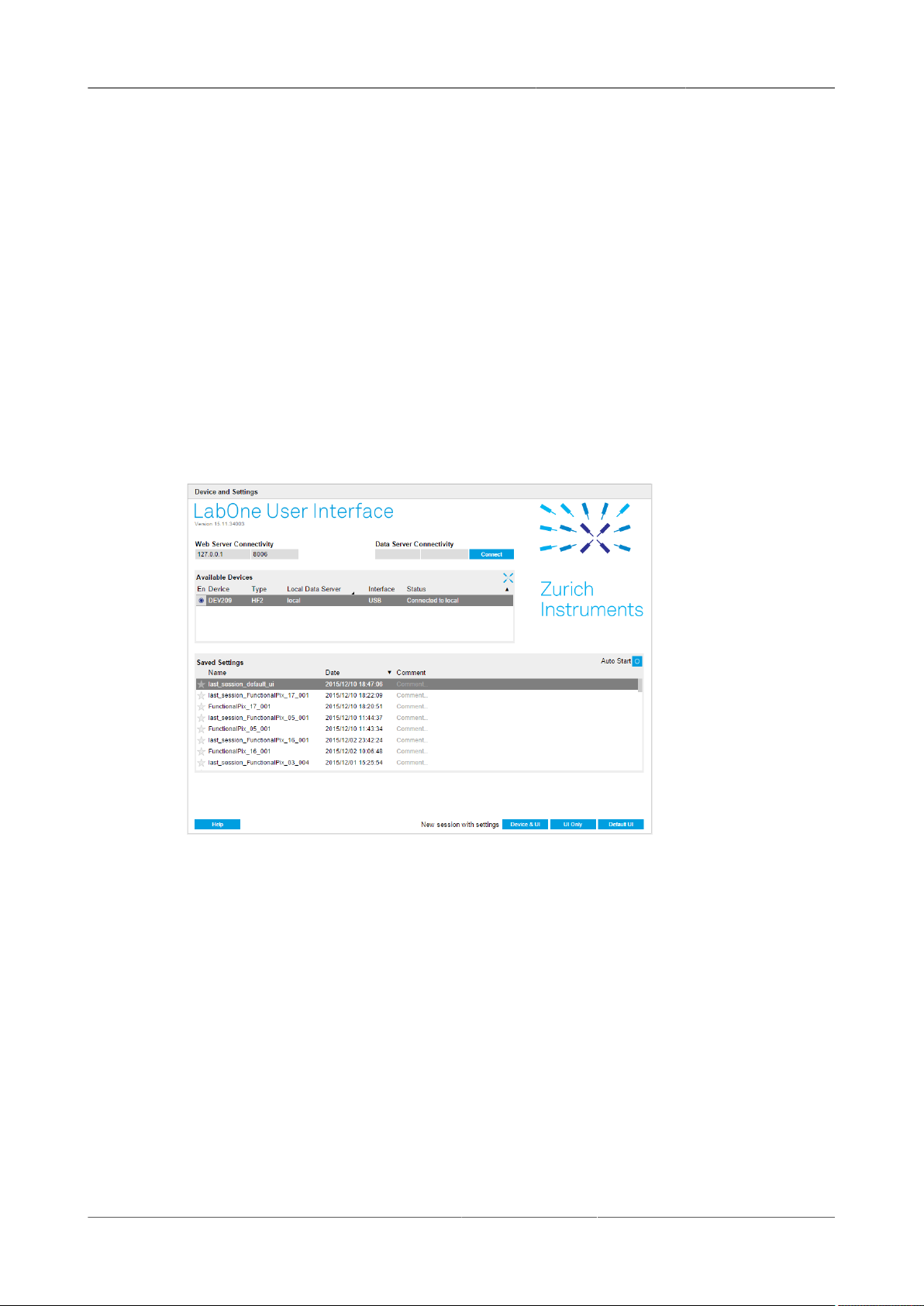
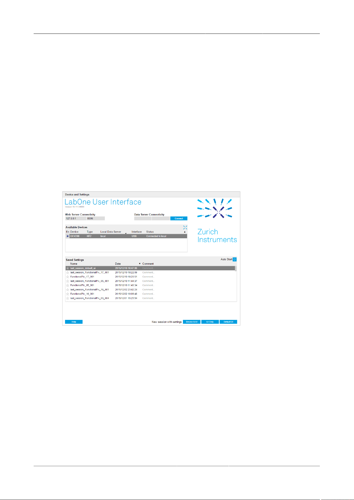
5. Start the LabOne User Interface. This will open the Device and Settings dialog in your default web browser. Your Instrument appears in the list of Available Devices. An example of the Device and Settings dialog is shown below.

6. Click the Default UI button on the bottom right of the page. The default configuration will be loaded and the first measurements can be taken. If the user interface does not start up successfully, please refer to Section1.5.3.

If any problems are encountered whilst setting up the instrument and software please see the

troubleshooting section at the end of this chapter.

Once the Instrument is up and running we recommend to go through some of the tutorials given in Chapter3. Moreover, Chapter2 provides a general introduction to the various tools and settings tabs with tables in each section providing a detailed description of every UI element as well. For specific application know-how the Blog section [www.zhinst.com/blogs/] of the Zurich Instruments web page will serve as a valuable resource that is constantly updated and expanded.

HF2 User Manual - LabOne Edition Revision 34390 Zurich Instruments 7

Page 8

1.2. Inspect the Package Contents

1.2.Inspect the Package Contents

If the shipping container appears to be damaged, keep the container until you have inspected the contents of the shipment and have performed basic functional tests.

You must verify that:

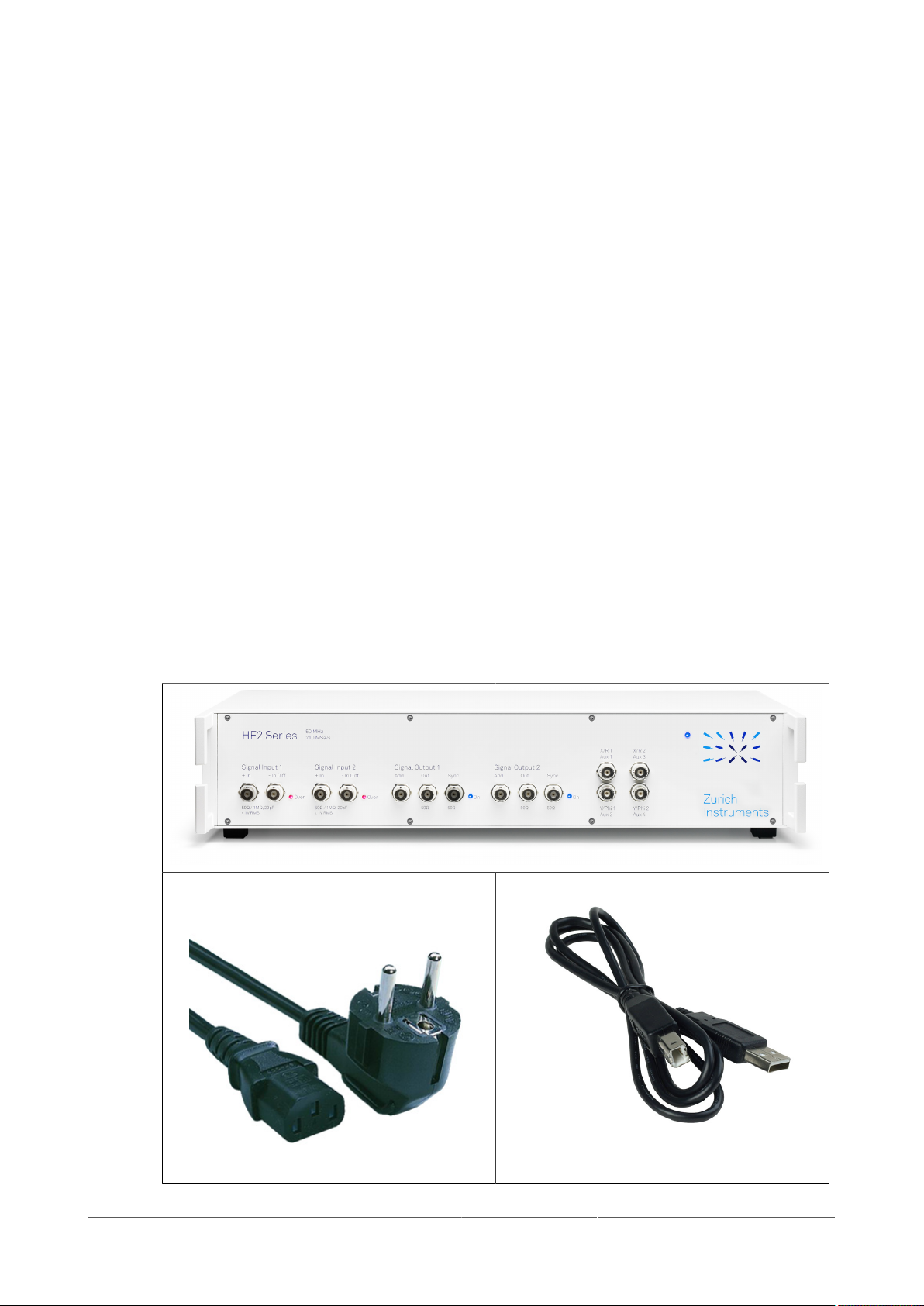
• You have received 1 Zurich Instruments HF2 Instrument

• You have received 1 power cord with a power plug suited to your country

• You have received 1 USB cable

• A printed version of the "Getting Started" section

• Additional cables have been added to the delivery if an HF2 pre-amplifier has been delivered

at the same time

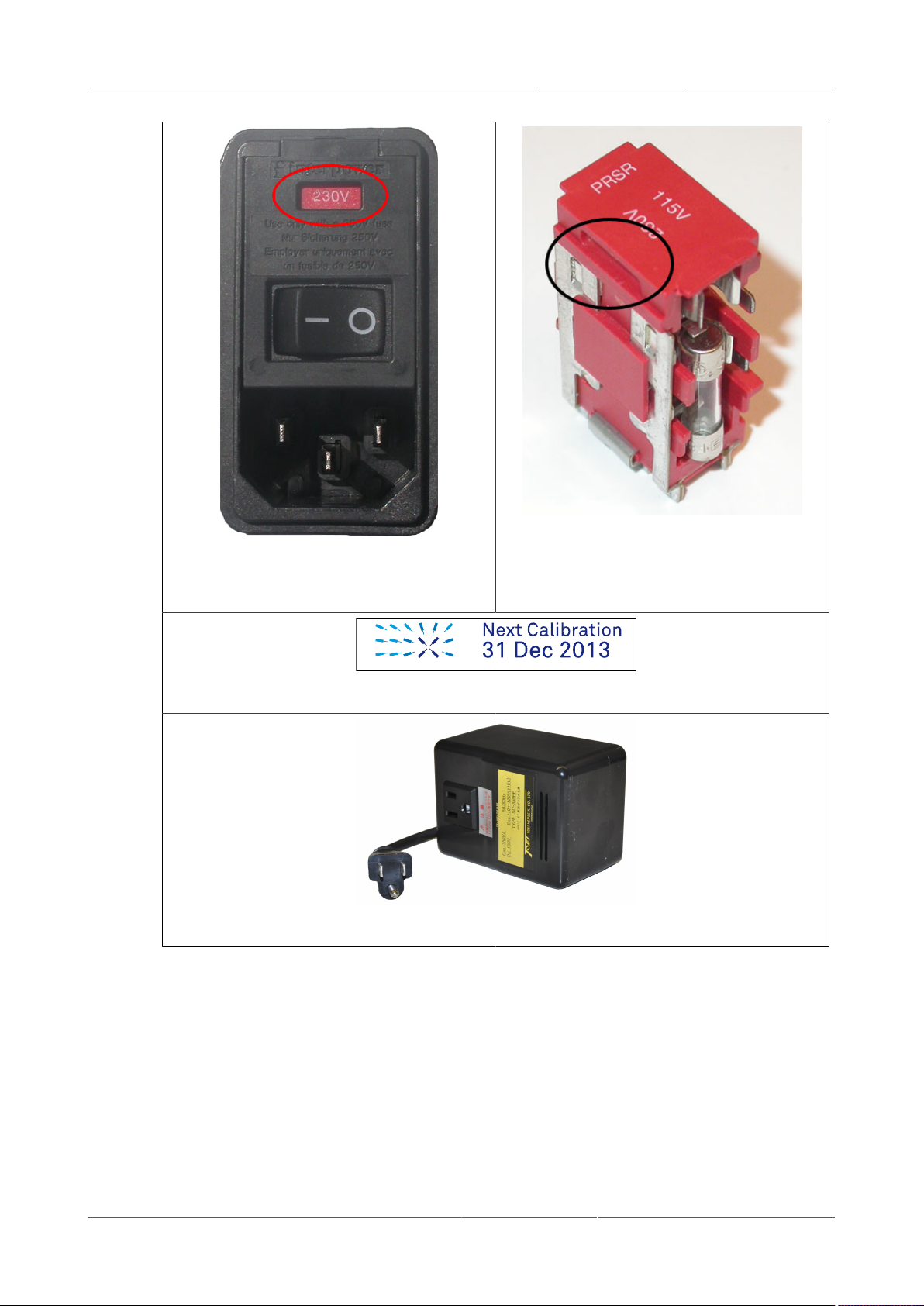
• The line voltage selector on the HF2 Instrument power inlet indicates the correct line voltage

of your country (115 V/60 Hz, or 230 V/50 Hz). While Zurich Instruments configures the power system when an instrument is initially delivered, no liability derives from potential wrong configuration or incorrect configuration at any point in time during the lifetime of the instrument

• The "Next Calibration" sticker on the rear panel of the Instrument indicates approximately 2

years ahead in time. Zurich Instruments recommends calibration intervals of 2 years

• For Japanese users only: you are supposed to operate the HF2 Instruments with an external

100 V to 110 V transformer in order to have reliable measurement results. Please verify having received the transformer included in your delivery from the local distributor.

Table1.1.Package contents for HF2 Instruments

Power cord USB cable

HF2 User Manual - LabOne Edition Revision 34390 Zurich Instruments 8

Page 9

1.2. Inspect the Package Contents

Fuse holder - requires 2 x 20 mm fast-

Power inlet with selected

230 V/50 Hz power system

The "Next Calibration" sticker on the rear panel of your instrupment

Japanese users only: the 100 V to 110 V transformer

Carefully inspect your HF2 Instrument. If there is mechanical damage or the instrument does not seem to operate after the software installation, please consult the handling instructions , then notify the Zurich Instruments support team at <[email protected]> as soon as possible.

acting fuses with 0.4 current limit - to extract

the fuse holder use a small screwdriver in

the indicated spot to lift it out of the casing

HF2 User Manual - LabOne Edition Revision 34390 Zurich Instruments 9

Page 10

1.3. Software Installation

1.3.Software Installation

HF2 Instruments are not stand-alone devices and require a PC with Zurich Instruments software installed. This section lists the software requirements and describes the installation process on Windows and Linux. Instructions for downloading the correct version of the software packages from the Zurich Instruments website are described below in the platform dependent sections.

1.3.1.Which User Interface: ziControl or the LabOne User Interface?

Up to and including software release 15.05, ziControl was the standard user interface (UI) shipped with HF2 Instruments. From 15.11 onwards HF2 Instruments ship with the LabOne User Interface, a browser-based UI. The ziControl UI is available to all users and the LabOne User Interface is available to users who have the WEB Option installed on their device. HF2 instruments shipped with release 15.11 onwards have the WEB Option installed by default. The WEB Option may be activated for other HF2 Instruments.

If the HF2 instrument does not have the WEB Option installed, then ziControl should be used as the user interface for the device and must be additionally installed as a separate package. In this case please refer to the "ziControl Edition" of the HF2 User Manual, ziControl installation is detailed there. The LabOne User Interface is included in the LabOne software package and does not require a separate installation.

1.3.2.Windows Installation

Requirements

Please ensure that the following requirements are fulfilled before trying to install the LabOne software:

1. Your PC is running a version of Windows supported by Zurich Instruments. Currently both 32bit and 64-bit architectures are supported on:

• Windows XP,

• Windows Vista,

• Windows 7, and

• Windows 8.

2. You have Windows administrator rights on the target system. Note after installation administrator rights are not required to run the Zurich Instruments software.

3. The correct version of the LabOne installer for your operating system and platform have been downloaded from the Zurich Instruments downloads page [http://www.zhinst.com/ downloads] (login required):

• LabOne<platform>-<release>.<revision>.msi, for example:

LabOne64-14.08.26000.msi

Please ensure you download the correct architecture (32-bit/64-bit) of the LabOne installer. In order to determine which architecture is required see the the section called “Determining

the PC Architecture on Microsoft Windows”.

HF2 User Manual - LabOne Edition Revision 34390 Zurich Instruments 10

Page 11

1.3. Software Installation

After ensuring that the requirements above are fulfilled, please proceed to first install the LabOne package as described in the section called “Windows LabOne Installation”

Note

In the naming convention the <platform> refers to the Windows addressing mode (32-bit: win32, 64-bit: win64), <release> refers the to software release as published by Zurich Instruments, and <revision> refers to the revision tag (which as no particular meaning for the user).

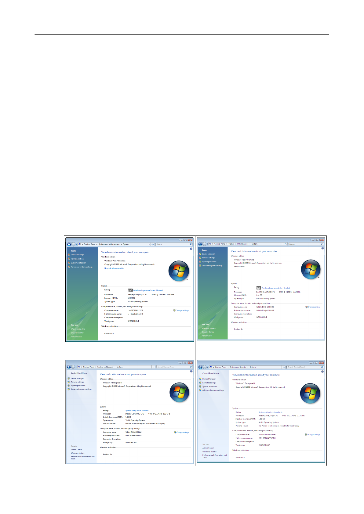
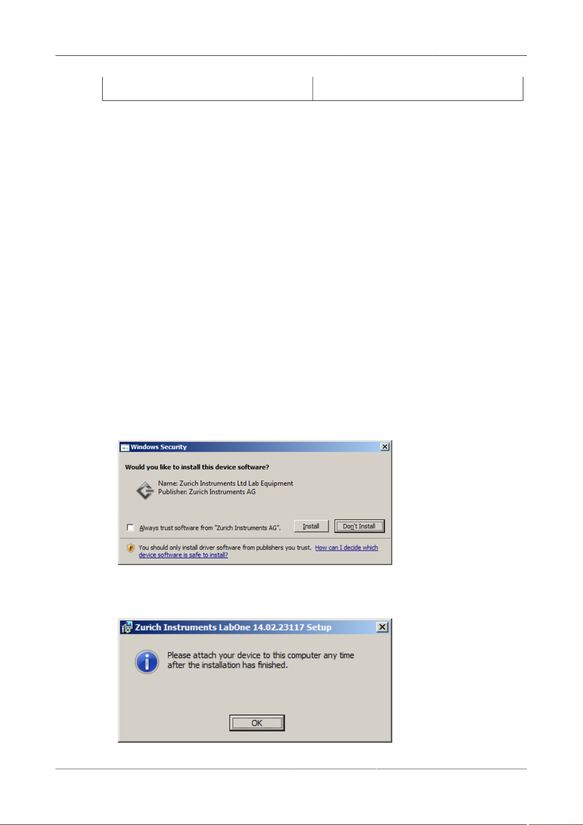
Determining the PC Architecture on Microsoft Windows

You can determine which architecture you are using as follows:

• Windows Vista: Control Panel → System and Maintenance → System / System type

• Windows 7: Control panel → System and Security → System / System type

• Windows 8: Control panel → System → System / System type

In general, x86 indicates a 32-bit system and x64 indicates a 64-bit operating system.

Table1.2.Determining the PC's platform architecture (32-bit/64-bit).

Windows Vista (32-bit: x86)

Windows Vista (64-bit: x64)

HF2 User Manual - LabOne Edition Revision 34390 Zurich Instruments 11

Page 12

1.3. Software Installation

Windows 7 (32-bit: x86) Windows 7 (64-bit: x64)

Windows LabOne Installation

1. The HF2 Instrument should not be connected to your computer during the installation process

2. Start the msi windows-installer program and follow the instructions. Please note that your windows user account needs to have administrator rights for this action. The installation proceeds as follows:

• On the welcome screen click the "Next" button

• After reading through the Zurich Instruments end-user license agreement, check the "I

accept the terms in the License Agreement" check box and click the "Next" button

• Review the features you want to have installed and then click the "Next" button - it is

recommended to install the complete package

• Click the "Install" button to start the installation process

• Accept the installation of new software (up to 3 pop-up windows) on your computer

including the installation of USB device drivers - you may decide to select the "Always trust software from Zurich Instruments AG" switch

• A message box appears reminding to complete the installation of the software by

connecting the HF2 Instrument to the computer by means of the USB cable - click the "OK" button

Figure1.1. Pop-up Window 1: Confirm to install the USB drivers (up to two times).

3. Click "Finish" to close the installer

Figure1.2. Pop-up Window 2: Click 'OK' to finish the installation.

HF2 User Manual - LabOne Edition Revision 34390 Zurich Instruments 12

4. Complete the LabOne installation process as follows:

Page 13

1.3. Software Installation

• The HF2 Instrument should not be connected to your computer during the installation

process

• Connect the power cord to the power input on the rear panel of the device and to a suited

AC power outlet

• Turn on the HF2 Instrument by means of the power switch on the back panel. Check if the

blue power indicator LED on the front panel is lit

• Connect the HF2 to the host computer with the provided USB cable. You need to have

administrator rights to finish the installation of the software. You may have to click through the common installation screens on older versions of Windows. In this step the installation of the USB driver completes

When the installation is completed, and every time you re-connect the instrument to your computer, the red "Over" LEDs on the HF2 front panel will blink 10 times to indicate that a functional computer connection is established. The HF2 Instrument is now powered on, and ready to be used.

With the installation of the LabOne package, you will be able to access the documentation: Windows → Zurich Instruments → Documentation → User Manual HF2.

64-bit Windows Installer Issue

In seldom cases the Windows Installer Service may be corrupted resulting in error message:

The Windows Installer Service could not be accessed. This can occur if the Windows Installer is not correctly installed. Contact your support personnel for assistance.

Assuming the Windows Installer itself is installed (which is the case on most Windows systems), this problem can be caused by the 32-bit service being started instead of the 64-bit version. To resolve this issue, the following steps have to be performed:

1. Start the cmd command prompt with administrator privileges.

2. Run the command net stop MSIServer in the cmd window to stop the service.

3. Run the regedit Windows Registry Editor.

4. Locate the key

HKEY_LOCAL_MACHINE\SYSTEM\CurrentControlSet\services\MSIServer

and set the value of the entry WOW64 to 0.

5. Close the Windows Registry Editor and execute the command net start MSIServer in the cmd window to restart the service. Confirmation of a successful service start should be printed and the installation of 64-bit software should be possible again.

1.3.3.Linux Installation

Requirements

HF2 User Manual - LabOne Edition Revision 34390 Zurich Instruments 13

Page 14

1.3. Software Installation

Please ensure that the following requirements are fulfilled before trying to install the software:

1. Officially, only Ubuntu 12.04 LTS (i386, amd64) is supported although in practice the Zurich Instruments software could work on other platforms. Please ensure that you are using a Linux distribution that is compatible with Ubuntu/Debian, but preferably Ubuntu 12.04 LTS.

2. You have administrator rights for the system.

3. The correct version of the LabOne installation package for your operating system and platform have been downloaded from the Zurich Instruments downloads page [http://www.zhinst.com/ downloads] (login required):

• LabOneLinux<arch>-<release>.<revision>.tar.gz, for example:

LabOneLinux64-14.08.26000.tar.gz

Please ensure you download the correct architecture (32-bit/64-bit) of the LabOne installer. The uname command can be used in order to determine which architecture you are using, by running:

uname -m

in a command line terminal. If the command outputs "x686" the 32-bit version of the LabOne package is required, if it displays "x86_64" the 64-bit version is required.

Linux LabOne Installation

Please proceed with the installation in a command line shell as follows:

1. Extract the LabOne tarball in a temporary directory:

tar xzvf LabOneLinux<arch>-<release>-<revision>.tar.gz

2. Navigate into the extracted directory.

cd LabOneLinux<arch>-<release>-<revision>

3. Run the install script with administrator rights and proceed through the guided installation, using the default installation path if possible:

sudo bash install.sh

The install script lets you choose between the following three modes:

• Type "a" to install the Data Server program, documentation and APIs.

• Type "u" to install the udev support.

• Type "ENTER" to install both the options "a" and "l" (recommended).

4. Optional: If udev was not installed, the Data Server program for the HF2 "ziServer" should be started manually:

ziServer &

5. Optional: If udev was installed, then the Data Server program does not have to be started manually, it will be started upon plugging in the USB cable of the HF2 and powering on the device. In this case the ziService program will also have been installed which can be used to control ziServer (with administrator rights).

sudo ziService [start,stop,update,status]

HF2 User Manual - LabOne Edition Revision 34390 Zurich Instruments 14

Page 15

1.3. Software Installation

Important

Do not use two ziServer instances running in parallel. If you have udev support installed, ziServer is started the first time you are powering on a HF2 Instrument (hot plug). It is not necessary to manually start the program.

Uninstalling the LabOne Software on Linux

Both software packages copy an uninstall script to the base installation paths (the default installation directory is /opt/zi/). To uninstall the packages please proceed in a command line shell as follows:

1. Navigate to the base installation path of LabOne, if the default path is used:

cd /opt/zi/

2. Run the uninstall scripts with administrator rights and proceed through the guided steps:

sudo bash uninstall_LabOne<arch>-<release>-<revision>.sh

HF2 User Manual - LabOne Edition Revision 34390 Zurich Instruments 15

Page 16

1.4. Handling and Safety Instructions

1.4.Handling and Safety Instructions

The HF2 Instrument is an electronic device. It is seriously discouraged to open the device, as there are high-voltage parts inside which may be harmful to human beings. There are no serviceable parts inside the device. Opening the device immediately cancels the warranty as provided by Zurich Instruments.

The following general safety instructions must be observed during all phases of operation, service, and handling of the instrument. The disregard of these precautions and all specific warnings elsewhere in this manual may affect correct operation of the equipment and its lifetime.

Zurich Instruments assumes no liability for the user's failure to observe and comply with the instructions in this user manual.

Table1.3.Safety Instructions

Ground the instrument The chassis must be correctly connected to

earth ground by means of the supplied power cable. Alternatively also the ground pin on the rear panel can be used. This avoids electrical shocks and potential damage to the instrument. For more information on ground and earth scheme, refer to section Section8.5).

Maximum ratings The specified electrical ratings for the

connectors of the instrument should not be exceeded at any time during operation (please

refer to section Section8.1). Do not service or adjust anything yourself There are no serviceable parts inside Software updates Regular software updates provide the user

with many important bug fixes, but also with

many new features. Only the last released

software version will be supported by Zurich

Instruments Overseas travel Consider that a power system change without

changing the orientation of the fuse holder

will damage the fuses, or make the instrument

behaving unpredictably Warnings Instructions contained in any warning issued

by the instrument, either by the software, the

graphical user interface, or mentioned in this

manual must be followed Notes Instructions contained in the notes of this

user manual are of essential importance for

the correct interpretation of the acquired

measurement data Location and ventilation Keep and operate the HF2 Instrument in a dry

location that suits the general specifications.

Do not block the ventilator opening on the back

or the air intake on the side of the chassis and

allow a reasonable space for the air to flow RJ45 plugs Although the device has several RJ45 plugs,

these are not intended for Ethernet connection.

Connecting these plugs with an Ethernet device

HF2 User Manual - LabOne Edition Revision 34390 Zurich Instruments 16

Page 17

1.4. Handling and Safety Instructions

Operation and storage Do not operate or store at a location outside

Handling Do not throw the HF2 Instrument, handle with

When you notice any of the situations listed below, immediately stop the operation of the HF2 Instrument, disconnect the power cord, and contact the support team at Zurich Instruments, either through the website form or by email at <[email protected]>.

Table1.4.Unusual Conditions

Fan is not working properly or not at all Operation must be avoided to prevent

Power cord or power plug on instrument is damaged

Instrument emits abnormal noise, smell, or sparks

may damage the HF2 Instrument and/or the

Ethernet device

the specified ambient conditions (please refer

to section Section8.3).

due care, do not store liquids on the device as

there is a chance of spilling and damage

overheating of sensitive electronic components

Operation must be avoided in order to prevent

overheating, electric shock, or fire. Please

exchange the power cord with a quality product

Operation must be avoided to prevent large

damage

HF2 User Manual - LabOne Edition Revision 34390 Zurich Instruments 17

Page 18

1.5. Connecting to the Instrument

Device 1 Device 2 Device 3

ziDAQ API

Application Layer

API Layer (DLL)

Web Server Layer

ziPython API API

Web Browser Web Browser Matlab Python LabView

LabOne Web Server

Session Session

API Session API Session API Session API Session

Data Server LayerLabOne Data Server

Devices

USB

TCP : 8010

UDP : 8013

TCP : 8004

TCP : 8006

TCP : 8004

Data

1.5.Connecting to the Instrument

After the LabOne software has been installed, the HF2 instrument is ready to be connected to a PC by using the USB cable. This section gives you detailed instructions about the different possibilities of setting up the connection and start working with your instrument.

1.5.1.LabOne Software Architecture

The Zurich Instruments LabOne software gives quick and easy access to the instrument from a host PC. LabOne also supports advanced configurations with simultaneous access by multiple software clients (i.e., LabOne User Interface clients and/or API clients), and even simultaneous access by several users working on different computers. Here we give a brief overview of the architecture of the LabOne software. This will help to better understand the following chapters.

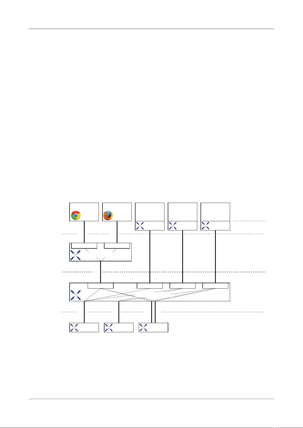
The software of Zurich Instruments lock-in amplifiers is server based. The servers and other software components are organized in layers as shown in Figure1.3. The lowest layer running on the PC is the LabOne Data Server which is the interface to the connected lock-in amplifier. The middle layer contains the LabOne Web Server which is the server for the browser-based LabOne User Interface. This graphical user interface, together with the programming user interfaces, are contained in the top layer. The architecture with one central Data Server allows multiple clients to access a device with synchronized settings. The following sections explain the different layers and their functionality in more detail.

LabOne Data Server

Figure1.3.Software architecture

The LabOne Data Server program is a dedicated server that is in charge of all communication to and from the device. The Data Server can control a single or also multiple lock-in amplifiers.

HF2 User Manual - LabOne Edition Revision 34390 Zurich Instruments 18

Page 19

1.5. Connecting to the Instrument

It will distribute the measurement data from the instrument to all the clients that subscribe to it. It also ensures that settings changed by one client are communicated to other clients. The device settings are therefore synchronized on all clients. The LabOne Data Server is started automatically whenever a HF2 instrument is connected to a PC via USB. On a PC only a single instance of a LabOne Data Server should be running.

LabOne Web Server

The LabOne Web Server is an application dedicated to serving up the web pages that constitute the LabOne user interface. The user interface can be opened with any device with a web browser. Since it is touch enabled, it is possible to work with the LabOne User Interface on a mobile device like a tablet. The LabOne Web Server supports multiple clients simultaneously. That is to say that more than one session can be used to view data and to manipulate the instrument. A session could be running in a browser on the PC on which the LabOne software is installed. It could equally well be running in a browser on a remote machine.

With a LabOne Web Server running and accessing an instrument, a new session can be opened by typing in a network address and port number in a browser address bar. In case the Web Server runs on the same computer, the address is the localhost address (both are equivalent):

• 127.0.0.1:8006

• localhost:8006

In case the Web Server runs on a remote computer, the address is the IP address or network name of the remote computer:

• 192.168.x.y:8006

• myPC.company.com:8006

The most recent versions of the most popular browsers are supported: Chrome, Firefox, Edge, Safari and Opera.

LabOne API Layer

The lock-in amplifier can also be controlled via the application program interfaces (APIs) provided by Zurich Instruments. APIs are provided in the form of DLLs for the following programming environments:

• MATLAB

• Python

• LabVIEW

• C

The instrument can therefore be controlled by an external program and the resulting data can be processed there. The device can be concurrently accessed via one or more of the APIs and via

HF2 User Manual - LabOne Edition Revision 34390 Zurich Instruments 19

Page 20

1.5. Connecting to the Instrument

the user interface. This enables easy integration into larger laboratory setups. See the LabOne programming manual for further information. Using the APIs, the user has access to the same functionality that is available in the LabOne User Interface.

1.5.2.LabOne Software Start-up

This section describes the LabOne User Interface start-up. If the LabOne Software is not yet installed on the PC please follow the instructions in Section1.3 Software Installation. If the device is not yet connected by USB please find more information in Section1.5.3 Device Connectivity.

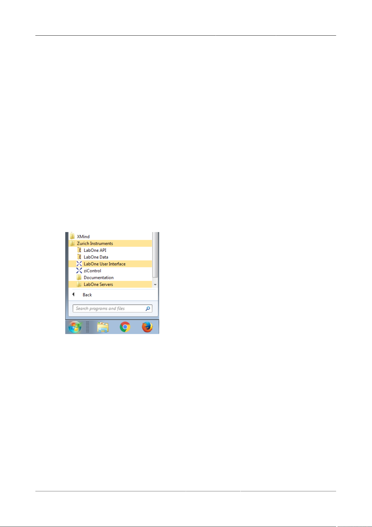
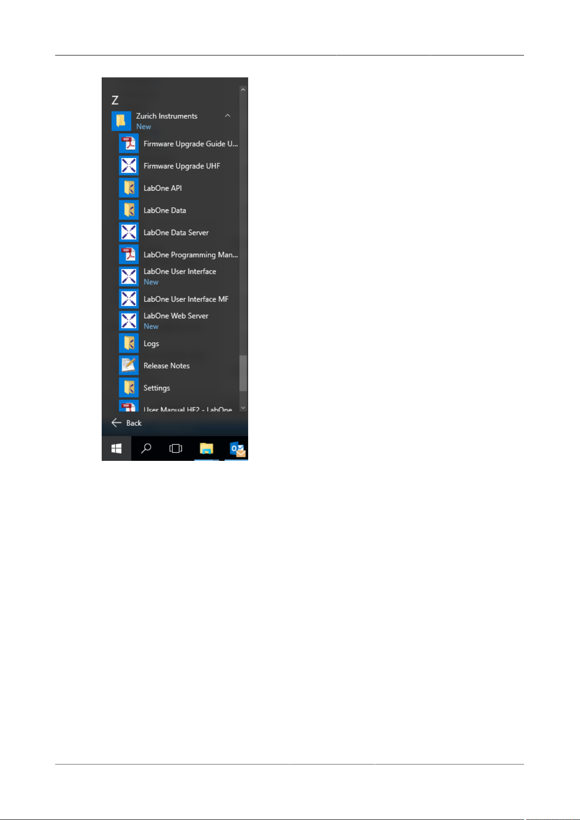
The most straightforward method to control and obtain data from the instrument is to use the LabOne User Interface, which can be found under the Windows Start Menu (see Figure1.4 and

Figure1.5): Click and select Start Menu → All programs / All apps → Zurich

Instruments → LabOne User Interface. This will open the User Interface in your default web browser and start the LabOne Data Server and LabOne Web Server programs in the background. A detailed description of the software structure is found in the Section 1.5.1 LabOne Software Architecture.

Figure1.4.Link to the LabOne User Interface in the Windows 7 Start Menu (All programs)

HF2 User Manual - LabOne Edition Revision 34390 Zurich Instruments 20

Page 21

1.5. Connecting to the Instrument

Figure1.5.Link to the LabOne User Interface in the Windows 10 Start Menu (All apps)

The LabOne User Interface is an HTML5 browser-based program. This simply means that the user interface runs in a web browser and that a connection using a mobile device is also possible; simply specify the IP address (and port 8006) of the PC running the user interface.

Note

The user interface requires the LabOne Web Server that runs in combination with the LabOne Data Server. Instead of starting the user interface in your default browser as described above, it's possible to start the LabOne Web Server program independently and then connect via a browser of your choice:

1. Start the LabOne Web Server program by selecting Start Menu → Programs → Zurich Instruments → LabOne Servers → LabOne Web Server. On Windows 10, you find the server in Start Menu → All Apps → Zurich Instruments → LabOne Web Server.

2. In a web browser of your choice start the LabOne User Interface by entering the localhost address with port 8006 to connect to the LabOne Web Server: 127.0.0.1:8006

HF2 User Manual - LabOne Edition Revision 34390 Zurich Instruments 21

Page 22

1.5. Connecting to the Instrument

Note

By creating a shortcut to Google Chrome on your desktop with the Target path\to\chrome.exe

-app=http://127.0.0.1:8006 set in Properties you run the LabOne User Interface in Chrome

in application mode which improves the user experience by removing the unnecessary browser controls.

Device and Settings Dialog

After starting the LabOne user interface software, a dialog is shown to select the device and settings for the session. The term session is used for an active connection between the user interface and the device. Such a session is defined by device settings and user interface settings. Several sessions can be started in parallel. The sessions run on a shared LabOne Web Server. A detailed description of the software architecture can be found in Section 1.5.1 Software Architecture.

Figure1.6.Dialog Device and Settings

The Device and Settings dialog consists of four sections: Web Server Connectivity, Data Server Connectivity, Available Devices, and Saved Settings. By default, the dialog is set to Local Data Server mode in the Available Devices section. In that case, the list of Available Devices will contain all instruments directly connected to the host PC via USB. The following steps are then required to start a new session

1. Select an instrument in the Available Devices list.

2. Select a setting file in the Saved Settings list unless the DefaultUI is used.

3. Start the session by clicking Device&UI, UIOnly, or DefaultUI

If there are no setting files listed, starting the LabOne User Interface by clicking the button DefaultUI will start a session using factory defaults.

HF2 User Manual - LabOne Edition Revision 34390 Zurich Instruments 22

Page 23

1.5. Connecting to the Instrument

Note

In case devices from other Zurich Instruments series (UHF, MF) are used in parallel, the list of Available Devices section can contain those as well.

Data Server Connectivity

The Device and Settings dialog represents a connection to a Web Server shown under Web Server Connectivity. However, on startup the Web Server is not yet connected to a LabOne Data Server, which is why the fields under Data Server Connectivity are empty. A connection to a Data Server can be opened by marking a device in the list of Available Devices and clicking the Connect button.

The Data Server Connect step is of little importance in case a single HF2 instrument on a single host computer is used. Data Server Connectivity is important for users working on an experiment from different control PCs, e.g. in the lab and in the office, and for HF2 users also working with devices from other Zurich Instruments series (UHF, MF).

To work with a HF2 instrument remotely, proceed as follows. On the computer directly connected to the HF2 (computer 1) open a user interface session and change the Connectivity setting in the Config tab to "From Everywhere", cf. Section4.13. On the remote computer (computer 2), open the Device and Settings dialog by starting up the LabOne User Interface. Change the dialog mode from Local Data Server to All Data Servers by opening the drop-down menu in the header row of the Available Devices table. This will make visible the HF2 device connected to computer 1. Select the device and connect to the remote Data Server by clicking on Connect. Then open the user interface as described above.

In case you use UHF or MF series instruments in parallel with the HF2, please refer to the UHF or MF documentation.

Note

When using All Data Servers mode, take great care to connect to the right instrument especially in larger local networks. Always identify your instrument based on its device serial of the form DEVXXXX which can be found on the instrument back panel.

Available Devices

The Available Devices section gives an overview of the visible devices. The first column of the list holds the Enable button controlling the connection between the device and a Data Server. For HF2 series instruments, this button is always greyed out since this connection is always established automatically.

The second column indicates the device serial and the third column shows the instrument type (HF2, UHF, or MFLI). The fourth column indicates shows the IP address of the LabOne Data Server controlling the device, if it is not a local one. The next column shows the interface type. For HF2 series instruments the interface type is always USB. The LabOne Data Server will scan for the available devices and interfaces once per second. If a device has just been switched on or physically connected it may take up to 20s before it becomes visible to the LabOne Data Server. If an interface is physically connected but not visible please read Section1.5.3 Device Connectivity. The last column indicates the status of the device which in the case of HF2 series instruments is always "Connected".

HF2 User Manual - LabOne Edition Revision 34390 Zurich Instruments 23

Page 24

1.5. Connecting to the Instrument

Saved Settings

Settings files can contain both UI and device settings. UI settings control the structure of the LabOne User Interface, e.g. the position and ordering of opened tabs. Device settings specify the set-up of a device. The device settings persist on the device until the next power cycle or until overwritten by loading another settings file.

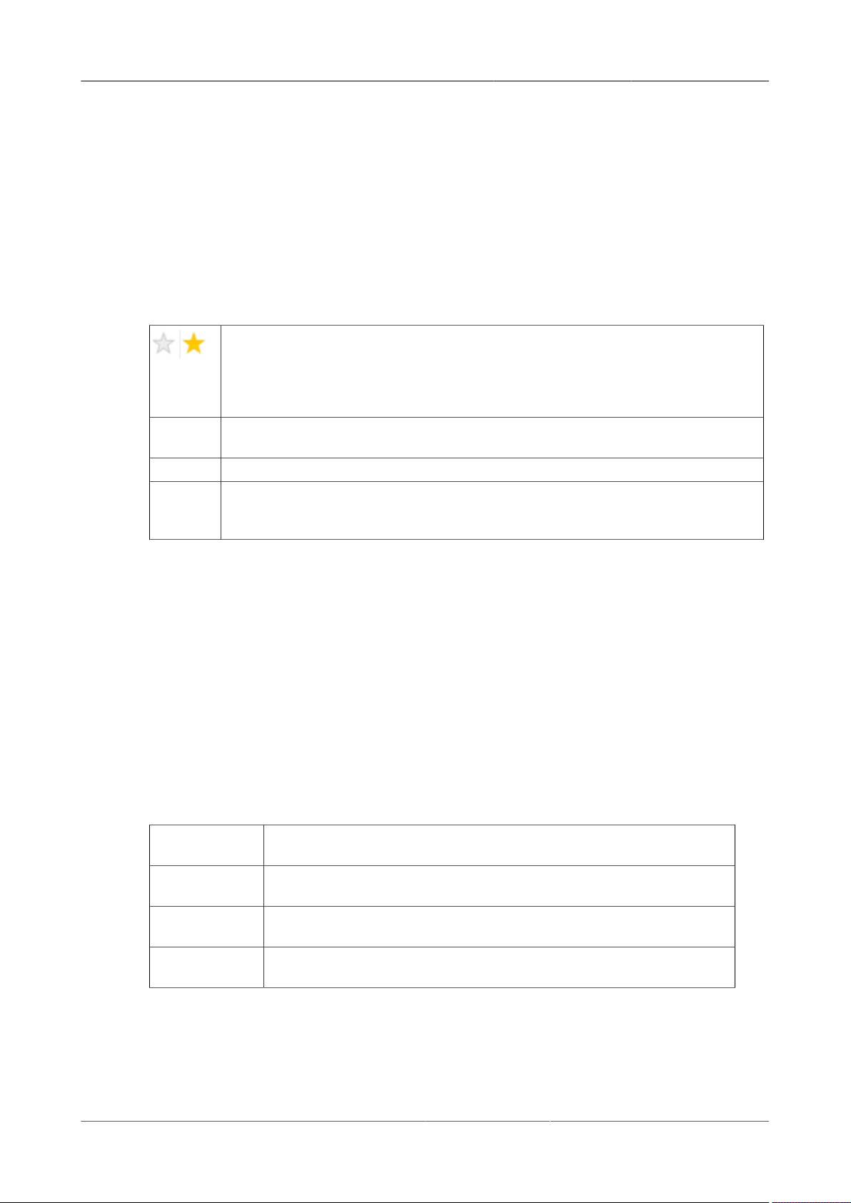
The columns are described in Table1.5. The table rows can be sorted by clicking on the column header that should be sorted. The default sorting is by time. Therefore, the most recent settings are found on top. Sorting by the favorite marker or setting file name may be useful as well.

Table1.5.Column Descriptions

Allows favorite settings files to be grouped together. By activating the stars adjacent to a settings file and clicking on the column heading, the chosen files will be grouped together at the top or bottom of the list accordingly. The favorite marker is saved to the settings file. When the LabOne user interface is started next time, the row will be marked as favorite again.

Name The name of the settings file. In the file system, the file name has the

extension .xml. Date The date and time the settings file was last written. Comment Allows a comment to be stored in the settings file. By clicking on the comment

field a text can be typed in which is subsequently stored in the settings file. This

comment is very useful to describe the specific conditions of a measurement.

Special Settings Files

Certain file names have the prefix "last_session_". Such files are created automatically by the LabOne Web Server when a session is terminated either explicitly by the user, or under critical error conditions, and save the current UI and device settings. The prefix is prepended to the name of the most recently used settings file. This allows any unsaved changes to be recovered upon starting a new session.

If a user loads such a last session settings file the "last_session_u" prefix will be cut away from the file name. Otherwise, there is a risk that an auto-save will overwrite a setting which was saved explicitly by the user.

The settings file with the name "default_ui" also has special meaning. As the name suggests this file contains the default UI settings. See button description in Table1.6.

Table1.6.Button Descriptions

Device & UI The Device and UI settings contained in the selected settings file will be

UI Only Only the UI settings contained in the selected settings file will be

Default UI Loads the default LabOne UI settings. The device settings remain

Auto Start Skips the session dialog at start-up if selected device is available. The

loaded.

loaded. The device settings remain unchanged.

unchanged.

default UI settings will be loaded with unchanged device settings.

Note

The factory default UI settings can be customized by saving a file with the name "default_ui" in the Config tab once the LabOne session has been started and the desired UI setup has been

HF2 User Manual - LabOne Edition Revision 34390 Zurich Instruments 24

Page 25

1.5. Connecting to the Instrument

established. To use factory defaults again, the "default_ui" file must be removed from the user setting directory.

Note

The user setting files are saved to an application-specific folder in the user directory structure. On Windows, the folder can be opened in a file explorer by following the link in the Windows Start Menu: Click and select Start Menu → Programs → Zurich Instruments → LabOne Servers → Settings.

Note

Double clicking on a device row in the Available Devices block is a quick way of starting the default LabOne UI. This action is equivalent to selecting the desired device and clicking the Default UI button.

Double clicking on a row in the Saved Settings block is a quick way of loading the LabOne UI with the those device and UI settings. This action is equivalent to selecting the desired settings file and clicking the Device & UI button.

Messages

The LabOne Web Server will show additional messages in case of a missing component or a failure condition. These messages display information about the failure condition. The following paragraphs list these messages and give more information on the user actions needed to resolve the problem.

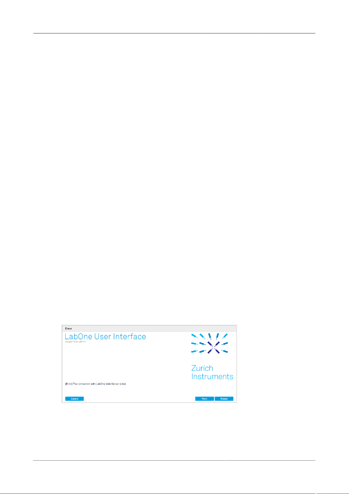
Lost Connection to the LabOne Web Server

In this case the browser is no longer able to connect to the LabOne Web Server. This can happen if the Web Server and Data Server run on different PCs and a network connection is interrupted. As long as the Web Server is running and the session did not yet time out, it is possible to just attach to the existing session and continue. Thus, within about 15 seconds it is possible with Retry to recover the old session connection. The Reload button opens the dialog Device and Settings shown in Figure1.6. The figure below shows an example of this dialog.

Figure1.7.Dialog: Connection Lost

Reloading...

HF2 User Manual - LabOne Edition Revision 34390 Zurich Instruments 25

Page 26

1.5. Connecting to the Instrument

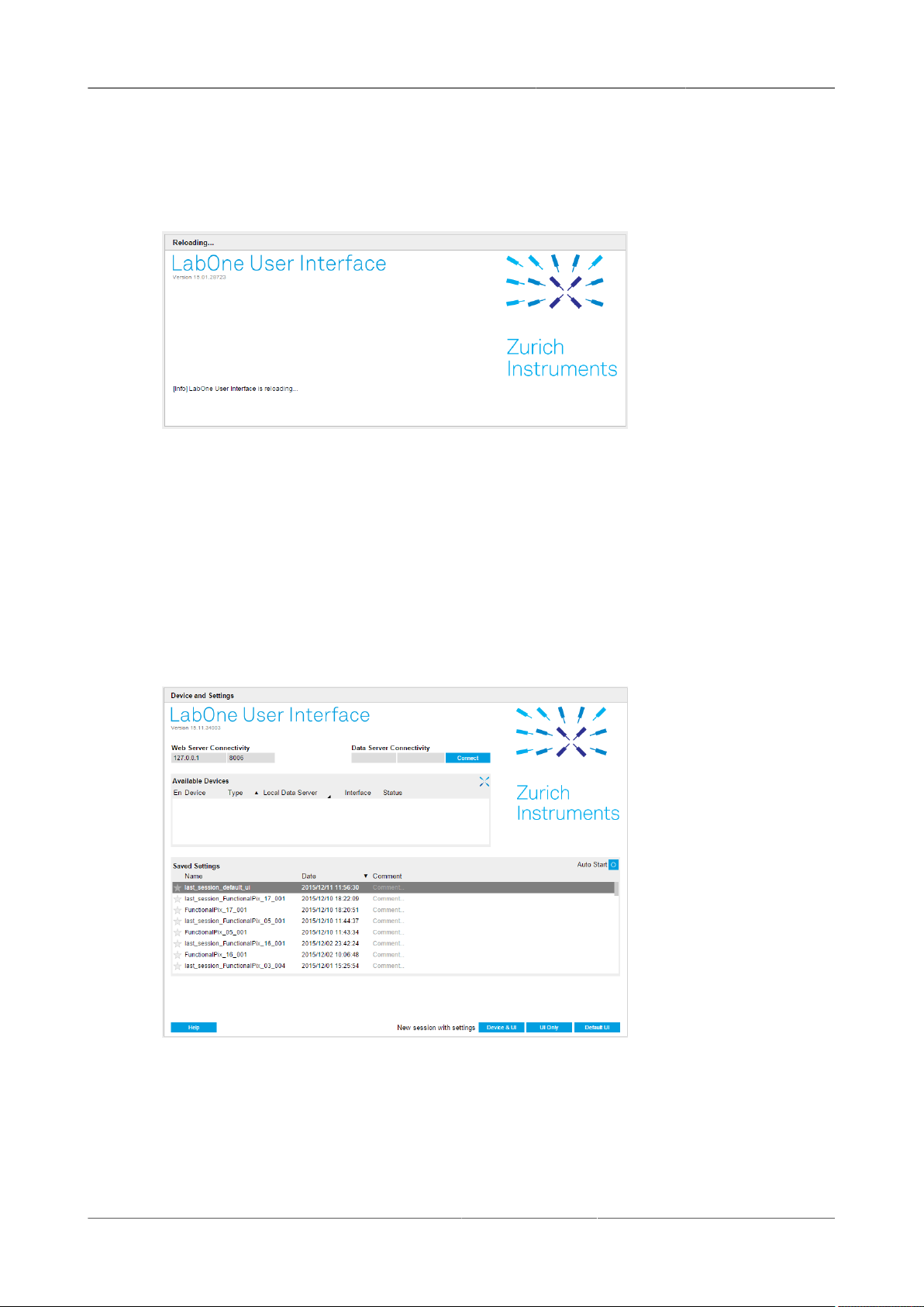
If a session error cannot be handled the LabOne Web Server will restart to show a new Dialog Device and Settings as shown in the section called “Device and Settings Dialog”. During the restart a window is displayed indicating that the LabOne User Interface will reload. If reloading does not happen the same effect can be triggered by pressing F5 on the keyboard. The figure below shows an example of this dialog.

Figure1.8.Dialog: Reloading

No Device Discovered

An empty "Available Devices" list means that no devices were discovered. This can mean that no LabOne Data Server is running, or that it is running but failed to detect any devices. The device may be switched off or the interface connection fails. For more information on the interface between device and PC see Section1.5.3 Device Connectivity. The figure below shows an example of this dialog.

Figure1.9.No Device Discovered

1.5.3.Device Connectivity

HF2 User Manual - LabOne Edition Revision 34390 Zurich Instruments 26

Page 27

1.5. Connecting to the Instrument

TCPIP Network

PC 2

PC 1

PC 3

Device 3

connected

Device 2

connected

Device 4

Device 1

connected

USB

TCPIP

USB visible USB connected TCPIP

USB

switch

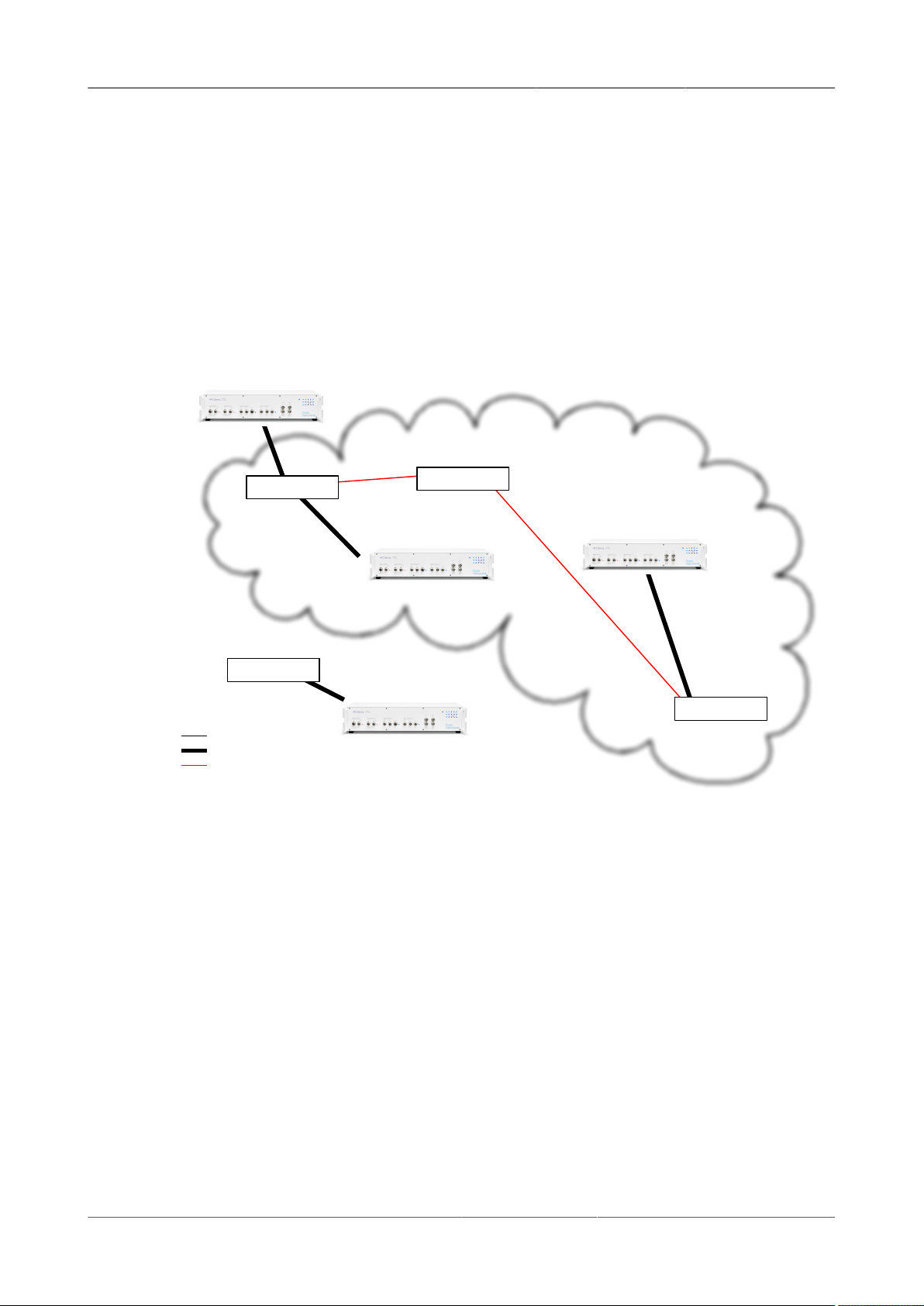
The device can be connected to a host computer by Universal Serial Bus (USB).The HF2 Instrument will then connect to the Data Server on the host PC. If the Data Server is not yet up and running, it is started up automatically when plugging in the USB connection. An instrument can be connected to one Data Server only, but a single Data Server and host computer can connect to several instruments at once.

If the host computer is in a local TCP/IP network, it's possible to control the device remotely and even from several computers simultaneously. Also in this remote configuration, there is a single LabOne Data Server connected to the instrument. This Data Server runs on the computer connected to the instrument via USB. The Data Server can serve one or more remote clients in the network. All clients can access the same measurement data. Changes in instrument settings done by one client will be seen by all other clients.

Figure1.10.Connectivity

Figure1.10 shows some examples of possible configurations of PC-to-device connectivity.

• Server on PC 1 is connected to device 1 (USB) and device 2 (USB).

• Server on PC 2 is connected to device 3 (USB).

• Server on PC 3 is connected to device 4.

• The devices 1, 2, and 3 are all visible to PC 1 and PC 2 over TCP/IP.

HF2 User Manual - LabOne Edition Revision 34390 Zurich Instruments 27

Page 28

1.6. Troubleshooting

1.6.Troubleshooting

This section aims to help the user solve and avoid problems whilst using the software and operating the instrument.

1.6.1.Common Problems

Your HF2 Instrument is an advanced piece of laboratory equipment with many more functionalities than a traditional lock-in amplifier. In order to benefit from these, the user needs access to a large number of settings in the LabOne User Interface. The complexity of the settings might overwhelm a first-time user, and even expert users can get surprised by certain combinations of settings. To avoid problems, it's good to use the possibility to save and load settings in the Config Tab. This allows one to keep an overview by operating the instrument based on known configurations. This section provides an easy-to-follow checklist to solve the most common mishaps.

The software cannot be installed or uninstalled: please verify you have Windows administrator rights. Windows systems: if prompted or required install the .NET Framework, see Section1.6.3.

The Instrument does not turn on: please verify the power supply connection and inspect the fuse. The fuse holder is integrated in the power connector on the back panel of the instrument.

The HF2 Instrument turns on but delivers obviously wrong measurements: please verify the power system setting on the back panel of the device is set to the power system of your country (110 V / 60 Hz, 220 V / 50 Hz). Make sure the fuse holder is set to the correct power supply position. This means that the wanted power supply label, 230 V or 115 V, must be positioned beside the edge of the power socket (e.g. not beside the power switch).

The HF2 Instrument performs poorly in a country with 100 V supply system (e.g. Japan): if no 100 V to 110 V transformer is used, the internal power supplies might be below specifications and some circuits might perform worse than specification. Users in countries with 100 V supply system are warmly recommended to use an external transformer (delivered with the instrument).

The HF2 Instrument shows limited data throughput on USB: although the host computer requirements are not particularly demanding, highest performance in USB throughput will require a performing desktop. The USB might be limiting the data throughput, please see Table8.4 for more details. Many concurrent transfers on the USB will limit the individual transfer. In particular the Scope should be turned off when not needed by the application. The status of the USB transfer can be monitored in the Status tab.

The Instrument performs poorly in single-ended operation: the signal inputs of the instrument might be set to differential operation. Please ensure that differential input mode is turned off in the Lock-in tab or In / Out tab.

The HF2 Instrument has a high input noise floor:the USB cable connects the Instrument ground to computer ground, which might inject some unwanted noise to the measurements results. In order to decouple the computer from the Instrument consider using an electrically isolating USB range extender supporting 480 Mbit/s data transfer rate (e.g. available from Icron Technologies). Be aware that the power supply of the range extender may need to be exchanged with a more stable power supply.

The Instrument performs poorly at low frequencies (below 10 kHz) : the signal inputs of the instrument might be set to AC operation. Please verify to turn off the AC switch in the Lock-in or In / Out tab.

The Instrument performs poorly during operation: the demodulator filters might be set too wide (too much noise) or too narrow (slow response) for your application. Please verify if the demodulator filter settings match your frequency versus noise plan.

HF2 User Manual - LabOne Edition Revision 34390 Zurich Instruments 28

Page 29

1.6. Troubleshooting

The Instrument performs poorly during operation: clipping of the input signal may be occurring. This is detectable by monitoring the red LEDs on the front panel of the instrument or the OVI flags on the status tab of the user interface. It can be avoided by adding enough margin on the input range setting (for instance 50% to 70% of the maximum signal peak).

The Instrument performs strangely when working with the HF2-MF Multi-frequency option: it is easily possible to turn on more signal generators than intended. Check the generated Signal Output with the integrated oscilloscope and check the number of simultaneously activated oscillator voltages.

The Instrument performs close to specification, but higher performance is expected: after 2 years since the last calibration, a few analog parameters are subject to drift. This may cause inaccurate measurements. Zurich Instruments recommends re-calibration of the Instrument every 2 years.

The Instrument measurements are unpredictable: please check the Status tab to see if any of the warning is occurring (red flag) or has occurred in the past (yellow flag).

The Instrument does not generate any output signal: verify that signal output switch has been activated in the Lock-in tab or In / out tab.

The Instrument locks poorly using the digital I/O as reference: make sure that the digital input signal has a high slew rate and clean level crossings.

The Instrument locks poorly using the auxiliary analog inputs as reference: the input signal amplitude might be too small. Use proper gain setting of the input channel.

The sample stream from the Instrument to the host computer is not continuous: check the sample loss (SL) and the packet loss (PL) flags in the status bar. The sample loss flag indicates occasional sample loss due to sampling rate set too high (the instruments sends more samples than the interface and the host computer can absorb). Reduce the sample rate settings. The packet loss indicates an important failure of the communications to the host computer and compromises the behavior of the instrument. Reduce the sample rate settings.

The Instrument is connected but there is no communication to the computer: check the clock fail (CF) flag in the status bar. This abnormal situation can occur if "Clk 10 MHz" is selected as Clock Source but no clock signal is fed to the Instrument. If Internal clock source is selected and the flag is still active, then the situation might indicate a serious hardware failure. In this case contact Zurich Instruments support team at <[email protected]>.

The user interface does not start or starts but remains idle: verify that the LabOne Data Server and LabOne Web Server have been started and are running on your host computer.

The user interface is slow and the web browser process consumes a lot of CPU power: make sure that the hardware acceleration is enabled for the web browser that is used for LabOne. For the Windows operating system, the hardware acceleration can be enabled in Control Panel\Display \Screen Resolution. Go to Advanced Settings and then Trouble Shoot. In case you use a NVIDIA graphics card, you have to use the NVIDIA control panel. Go to Manage 3D Settings, then Program Settings and select the program that you want to customize.

HF2 User Manual - LabOne Edition Revision 34390 Zurich Instruments 29

Page 30

1.6. Troubleshooting

1.6.2.Location of the log files

For Windows 7, 8, and 10 the log files are located in the following directories:

• LabOne Data Server: C:\Users\[USER]\AppData\Local\Temp\Zurich Instruments

\LabOne\ziDataServerLog

• LabOne Web Server: C:\Users\[USER]\AppData\Local\Temp\Zurich Instruments

\LabOne\ziWebServerLog

On Windows XP:

• LabOne Data Server: C:\Documents and Settings\[USER]\Local Settings\Temp

\Zurich Instruments\LabOne\ziDataServerLog

• LabOne Web Server: C:\Documents and Settings\[USER]\Local Settings\Temp

\Zurich Instruments\LabOne\ziWebServerLog

HF2 User Manual - LabOne Edition Revision 34390 Zurich Instruments 30

Page 31

1.6. Troubleshooting

1.6.3.Windows .NET Framework Requirement

The Zurich Instruments LabOne software installer requires the Microsoft .NET Framework to be installed on Windows systems. This is normally already installed on most Windows systems but may need to be additionally installed on some computers running Windows XP and Vista. If the .NET Framework is not available a message will be shown that this requirement is missing when the LabOne installer is started.

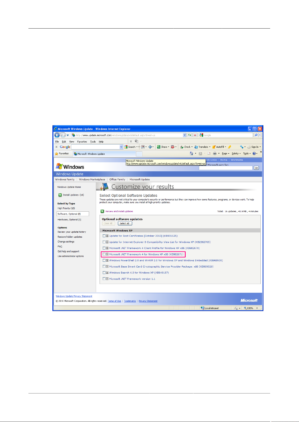
It is possible to check whether and which version of the Microsoft .NET Framework is installed on your system under Windows Start -> Control panel -> Add and Remove Programs. The minimum requirement is Microsoft .NET Framework 3.5 Service Pack 1. In case the required version is not installed, it can be installed through Windows Update tool (Windows Start -> Control panel -> Windows Update).

Figure1.11. Installation of the .NET Framework.

HF2 User Manual - LabOne Edition Revision 34390 Zurich Instruments 31

Page 32

Chapter2.Functional Overview

This chapter helps you to quickly get acquainted with the main features, the panels, and the operating modes of the HF2 Series. A product selector is provided listing the key features of the products in order to support the selection and ordering. This section is intended as overview and therefore has a coarse level of detail without containing detailed descriptions.

HF2 User Manual - LabOne Edition Revision 34390 Zurich Instruments 32

Page 33

2.1. Features

HF Signal Output 1

Output Range Amplifier

DAC 210 MS/s 16 bit

HF Signal Input 1

Input Range Amplifier

ADC 210 MS/s 14 bit

HF Signal Input 2

Input Range Amplifier

ADC 210 MS/s 14 bit

LPF 50 MHz

Auxiliary High-speed Outputs

4x DAC 1 MS/s 16 bit

LPF 200 kHz

Oscilloscope

Digital Signal Processor

Frequency Generator

Multi Numerical Oscillators

Output Mixers

Frequency Response Sweeper

LPF

Multi dual-phase demodulators

(X,Y)

Clock In 10 MHz

Clock Out 10 MHz

Internal Oscillator

HF2-UHS

(option)

Auxiliary High-speed Inputs

2x ADC 400 kS/s 16 bit

Digital I/O 32-bit

USB 2.0 High-speed

2x ZCtrl Pre-amplifier Bus

2x ZSync Synchronization Bus

Programmable 32-bit RISC Processor

HF2-RT (option)

HF2-MF

(option)

HF2-PLL

(option)

HF2-MOD

(option)

B a c k

P a n e

r o n

P a n e

HF Signal Output 2

Output Range Amplifier

DAC 210 MS/s 16 bit

LPF 50 MHz

LPF 100 kHz

FFT Spectrum Analyzer

HF2-PID Quad-PID (option)

2.1.Features

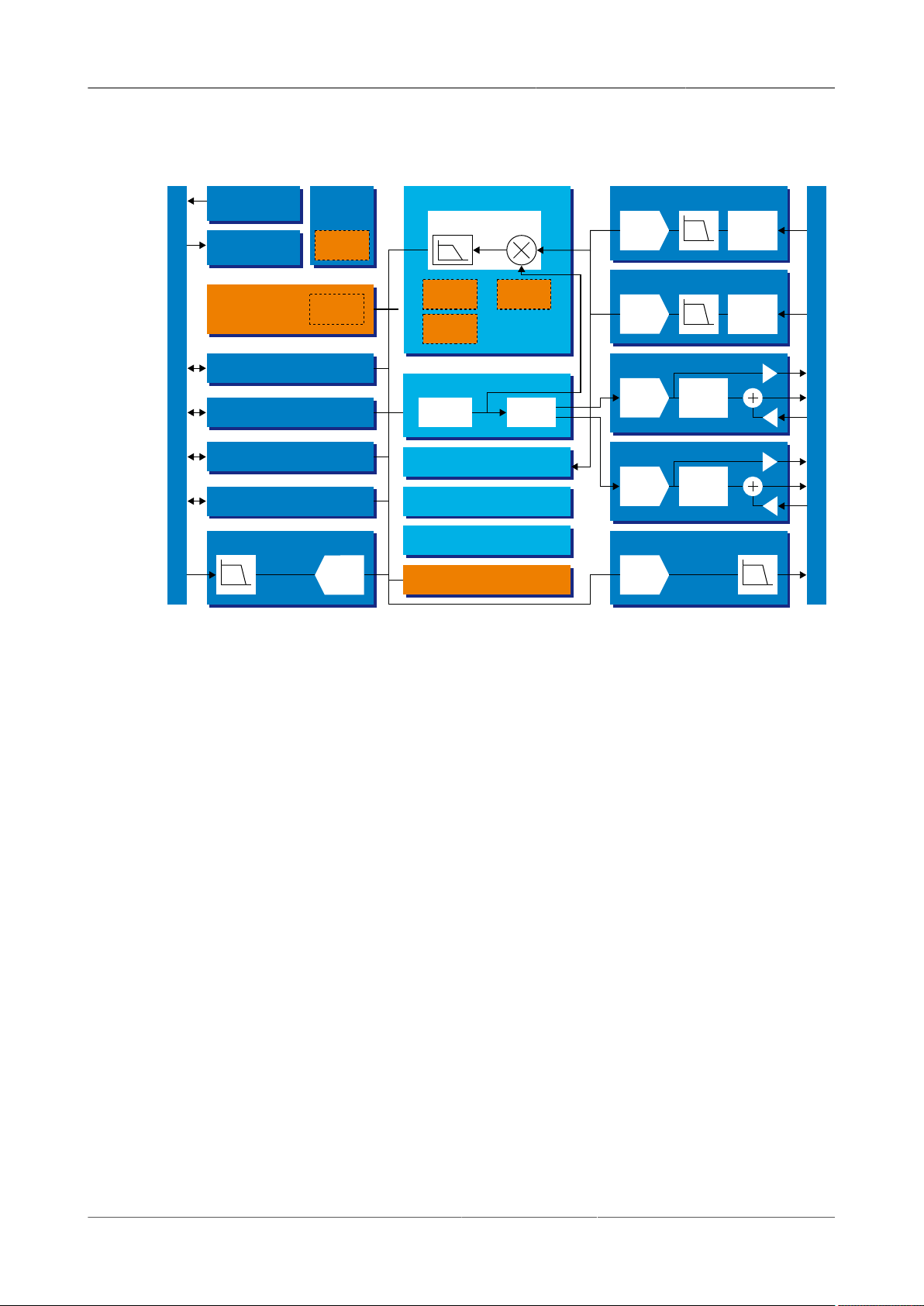
Figure2.1.HF2 functional diagram

The HF2 Instrument as in Figure2.1 consists of 4 high-frequency analog blocks, 2 low-frequency auxiliary blocks, the internal digital processing block (light-blue), and the hardware interfaces (mostly available on the back panel of the instrument).

The signal to be measured is connected to one of the two high-frequency analog inputs where it is amplified to a defined range, filtered, and digitized at very high speed. The resulting samples are fed into the digital signal processing block for demodulation by means of up to 8 dual-phase demodulators. The demodulators output samples flow into the embedded RISC processor for further processing or to be sent to the host computer. The samples are also sent to the auxiliary outputs in order to be available on the front panel of the HF2 Instrument.

The numerical oscillators generate sine and cosine signal pairs that are used for the demodulation of the input samples and also for the generation of the high-frequency output signals. For this purpose, the Output Mixers generate a weighted sum of the generator outputs to generate the multi-frequency signal that can be used a stimulation signal. The 2 high-frequency output stages provide analog to digital conversion, signal scaling (range), add of an external AC or DC signal, and a synchronization signal.

Operating Modes

• Internal reference mode

• External reference mode

• Auto reference mode

• Dual-channel operation

• Dual-harmonic mode

• Multi-harmonic mode

HF2 User Manual - LabOne Edition Revision 34390 Zurich Instruments 33

Page 34

2.1. Features

• Arbitrary frequency mode

High-frequency Analog Inputs

• 2 low-noise high-frequency inputs

• Differential & single-ended operation (A, -B, A-B)

• Variable input range

• Variable input impedance

• AC/DC coupling

High-frequency Analog Outputs

• 2 low-noise high-frequency outputs

• Large output range

• Variable output range settings

• 1 synchronization signal for each output

• 1 adder signal for each output

Auxiliary Analog Input/Outputs

• 4 auxiliary high-speed outputs

• 2 auxiliary high-speed inputs

• User defined signal on auxiliary output

Demodulators & Reference

• Up to 8 dual-phase demodulators

• Up to 8 programmable numerical oscillators

• Programmable demodulators filters

• Very-high resolution internal reference

• 64-bit resolution demodulator outputs

Measurement Tools

• Spectroscope

• Numerical

• Oscilloscope

• Frequency response analyzer

• FFT spectrum analyzer

User-programmable Embedded Processor (Option)

• Microblaze 32-bit RISC

• 64 MHz operation allows implementation of real-time control loops

• 32-bit floating-point unit

• 64 kB internal memory (maximum program size)

• 64 MB external memory DDR2

Other Interfaces

• USB 2.0 high-speed 480 Mbit/s host interface

HF2 User Manual - LabOne Edition Revision 34390 Zurich Instruments 34

Page 35

2.1. Features

• DIO: 32-bit digital input-output port

• ZSync: 2 ports for inter-instrument synchronization bus (ZI proprietary)

• ZCtrl: 2 ports for control/power bus for external pre-amplifiers (ZI proprietary)

• Clock input connector (10 MHz)

Software Features

• The LabOne User Interface, a powerful browser-based graphical interface

• ziServer multi-mode multi-connection server

• ziAPI for extended programmability in C, LabVIEW, MATLAB, and Python - programming

• Console: text interface to connect virtually any programming language

examples included

HF2 User Manual - LabOne Edition Revision 34390 Zurich Instruments 35

Page 36

2.2. Front Panel Tour

A B

D E

H I

K L M

A B

D E

H I

K L M

2.2.Front Panel Tour

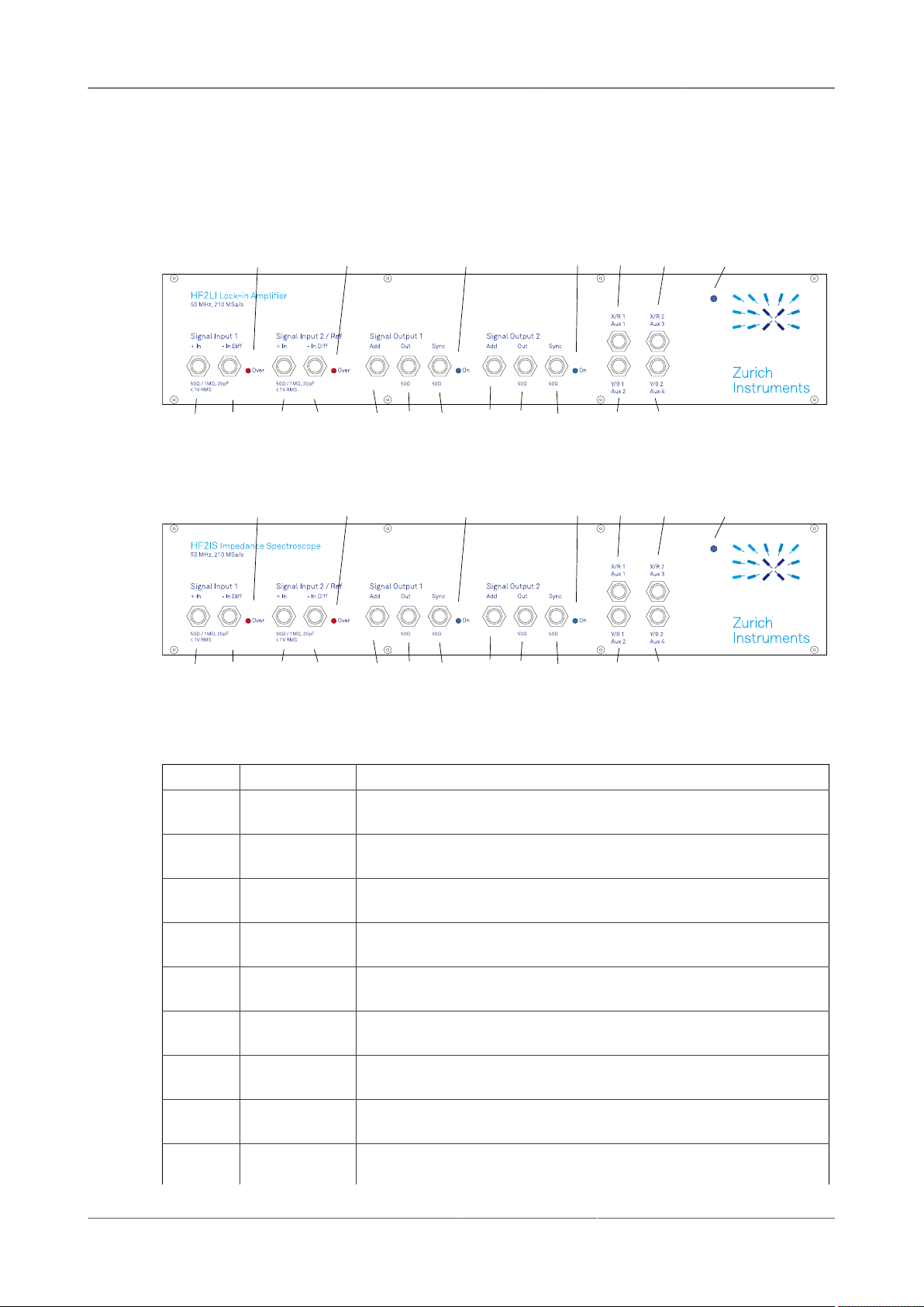
The front panel BNC connectors and control LEDs are arranged in 5 sections as shown in Figure2.2 and Figure2.3 listed in Table2.1. The HF2LI and HF2IS have the same connectors and connector functionality on their front- and back panel.

Figure2.2.HF2LI front panel

Figure2.3.HF2IS front panel

Table2.1.HF2 Series front panel description

Position Label / Name Description A Signal Input 1

+ In

B Signal Input 1 -

In Diff

C Signal Input 1

Over

D Signal Input 2 /

Ref + In

E Signal Input 2 /

Ref - In Diff

F Signal Input 2

Over

G Signal Output 1

Add

H Signal Output 1

I Signal Output 1

Out

Sync

single-ended input

negative input (when not used, has to be internally shorted to ground with switch on graphical user interface)

this LED indicates that the input signal saturates the A/D converter

single ended input / reference input for external reference mode

negative input (when not used, has to be internally shorted to ground with switch on graphical user interface)

this LED indicates that the input signal saturates the A/D converter

the signal applied to the connector is added (analog add) to the output signal

high-frequency output

the output signal before the output gain stage for use as synchronization or monitoring signal; the amplitude voltage

HF2 User Manual - LabOne Edition Revision 34390 Zurich Instruments 36

Page 37

2.2. Front Panel Tour

Position Label / Name Description

J Signal Output 1Onthis LED indicates that the signal output is turned on

calculates as ratio of the corresponding output amplitude and its range setting

K Signal Output 2

Add

L Signal Output 2

Out

M Signal Output 2

Sync

N Signal Output 2Onthis LED indicates that the signal output is turned on

O X/R 1 / Aux 1 this connector provides either the in-phase signal of the

P Y/Θ 1 / Aux 2 this connector provides either the quadrature signal of the

Q X/R 2 / Aux 3 this connector provides either the in-phase signal of the

R Y/Θ 2 / Aux 4 this connector provides either the quadrature signal of the

S Power instrument mains power-on LED

the signal applied to the connector is added (analog add) to the output signal

high-frequency output

the output signal before the output gain stage for use as synchronization or monitoring signal; the amplitude voltage calculates as ratio of the corresponding output amplitude and its range setting

demodulator (X1), the magnitude (R1), or an auxiliary output signal Aux 1

demodulator (Y1), the phase (Θ1), or an auxiliary output signal Aux 2

demodulator (X2), the magnitude (R2), or an auxiliary output signal Aux 3

demodulator (Y2), the phase (Θ2), or an auxiliary output signal Aux 4

HF2 User Manual - LabOne Edition Revision 34390 Zurich Instruments 37

Page 38

2.3. Back Panel Tour

C,D

B E,F

G,H

I,J L M N

2.3.Back Panel Tour

The back panel is the main interface for power, control, service and connectivity to other ZI instruments. Please refer to Figure2.4 and Table2.2 for the detailed description of the items.

Figure2.4.HF2 Series back panel

Table2.2.HF2 Series back panel description

Position Label / Name Description A - ventilator (important: keep clear from obstruction) B Earth ground 4 mm banana jack connector for earth ground purpose,

electrically connected to the chassis and the earth pin of the

power inlet C Power inlet power inlet with On/Off switch D Power system select between 115 V and 230 V power system E ZCtrl 1 peripheral pre-amplifier power & control bus 1 - attention: this

is not an Ethernet plug, connection to an Ethernet network might

damage the instrument F ZCtrl 2 peripheral pre-amplifier power & control bus 2 - attention: this

is not an Ethernet plug, connection to an Ethernet network might

damage the instrument G Aux In 1 auxiliary high-sampling rate input 1 H Aux In 2 auxiliary high-sampling rate input 2 I DIO 0 digital input/output 0 J DIO 1 digital input/output 1 K DIO digital input/output 0-31 L Clock In clock input (10 MHz) M ZSync In inter-instrument synchronization bus input - attention: this is

not an Ethernet plug, connection to an Ethernet network might

damage the instrument N ZSync Out inter-instrument synchronization bus output - attention: this is

not an Ethernet plug, connection to an Ethernet network might

damage the instrument O USB host computer connection

HF2 User Manual - LabOne Edition Revision 34390 Zurich Instruments 38

Page 39

2.4. Ordering Guide

2.4.Ordering Guide

The HF2 Series is a product line comprising an impedance spectroscope and a digital lock-in amplifier covering advanced requirements for laboratory equipment. The HF2 Series provides best-in-class performance, wide operation range, intuitive handling and excellent accuracy.

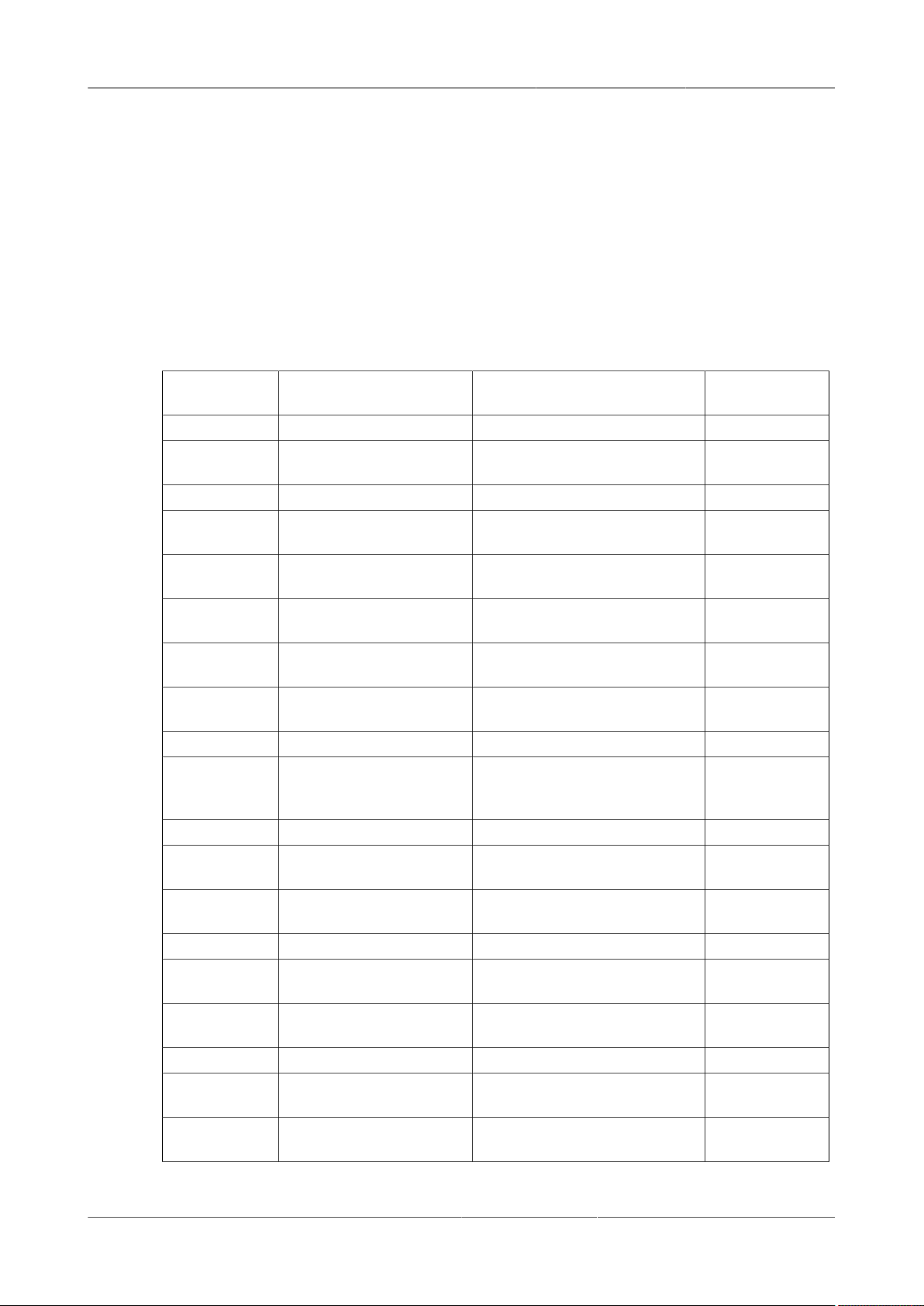
Table2.3 provides an overview of the available products in the HF2 Series. Upgradeable features

are options that can be purchased anytime without need to send the instrument to Zurich Instruments - the upgradeable features consist of a firmware upgrade.

Table2.3.HF2 Series product codes for ordering

Product code Product name Description Upgrade in the

HF2LI HF2LI Lock-in Amplifier base lock-in amplifier HF2LI-MF HF2LI-MF Multi-

frequency HF2LI-RT HF2LI-RT Real-time option yes HF2LI-PLL HF2LI-PLL Dual Phase-

locked Loop HF2LI-PID HF2LI-PID Quad PID

Controller HF2LI-MOD HF2LI-MOD AM/FM

Modulation HF2LI-UHS HF2LI-UHS Ultra-high

Stability HF2LI-WE2Y HF2LI-WE2Y Warranty

Extension 2 Years

- - - HF2PLL HF2PLL Phase-locked

Loop

- - - HF2IS HF2IS Impedance

Spectroscope HF2IS-MF HF2IS-MF Multi-

frequency HF2IS-RT HF2IS-RT Real-time option yes HF2IS-UHS HF2IS-UHS Ultra-high

Stability HF2IS-WE2Y HF2IS-WE2Y Warranty

Extension 2 Years

- - - HF2CA HF2CA Current Amplifier low noise current amplifier with

HF2TA HF2TA Current Amplifier low noise transimpedance

field possible

option yes

option no

warranty extension for 2 additional years

bundle of the HF2LI plus the HF2LI-PLL and the HF2LI-PID options

base impedance spectroscope -

option yes

option no

warranty extension for 2 additional years

adaptable input impedance

amplifier

yes

HF2 User Manual - LabOne Edition Revision 34390 Zurich Instruments 39

Page 40

2.4. Ordering Guide

Table2.4.Product selector

Feature HF2LI HF2LI +

HF2LI-MF Internal reference mode yes yes yes yes External reference mode yes yes - Auto reference mode yes yes - Dual-channel operation (2

independent measurement units) Sinusoidal generators 2 2 2 2 Superposed output sinusoidals per

generator Dual-harmonic mode yes yes - Multi-harmonic mode - yes - Arbitrary frequency mode - yes yes yes Number of demodulators 6 6 4 8 Simultaneous freq. supported

(fundamentals/harmonics) Signal input select switch matrix - yes yes yes Oscillator select switch matrix - yes - 50 MHz, 210 MS/s, 0.8 μs TC yes yes yes yes DSP technology 128 bit 128 bit 128 bit 128 bit Dynamic reserve 120 dB 120 dB - Lock-in range 50 MHz 50 MHz - USB 2.0 480 Mbit/s yes yes yes yes LabOne User Interface, ziAPI,

ziServer software Frequency response sweeper yes yes yes yes Oscilloscope yes yes yes yes

yes yes yes yes

1 up to 6 up to 4 up to 8

2/4 6/- 4/- 8/-

yes yes yes yes

HF2IS HF2IS +

HF2IS-MF

HF2 User Manual - LabOne Edition Revision 34390 Zurich Instruments 40

Page 41

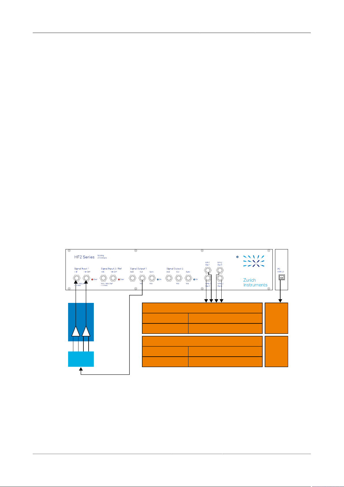
2.5. Operating Modes

Max 6 sample streams

DUT 1

HF2LI

HF2CA

Max 8 sample streams

HF2IS

drive signal

HF2LI sample output (any 2 of)

Input 1

Input 1 with MF

F1, H1a, H1b

F1, H1a, H1b, H1c, H1d, H1e

HF2IS sample output (any 2 of)

Input 1

Input 1 with MF

F1, F2, F3, F4

F1, F2, F3, F4, F5, F6, F7, F8

2.5.Operating Modes

2.5.1.Internal Reference Mode

The internal reference mode takes advantage of the internal HF generators inside the HF2 Instrument. There are 6 frequency generators in the HF2LI and up to 8 frequency generators in the HF2IS. The output of these generators are added numerically inside the instrument avoiding complicated external analog signal adders and the resulting signal is fed to the device under test. The internal reference mode is the preferred mode as the signal recovery works at its best as the generated frequency is known inside of the instrument. The signal acquisition works immediately and there is no delay lock-time.

The internal reference mode is supported with single-channel and dual-channel operation. This is possible as the HF2 Instrument includes 2 independent measurement units that are working autonomously. Each of the measurement units provides analysis for one fundamental and 2 harmonic frequencies in parallel (sometimes called dual-harmonic mode). In total, the HF2LI can measure 2 fundamental and 4 harmonic frequencies, while the HF2IS can measure 4 frequencies. The number of frequencies increases with the multi-frequency options.

The demodulator samples are available in analog format on the auxiliary outputs of the HF2 Instrument and digitally on the connected computer transferred over the USB interface. The auxiliary outputs generate an analog signal after a linear digital to analog conversion at high sample rate. There are 2 pairs of analog signals allowing to output any 2 of the demodulation sample streams. All demodulator streams are available on the computer and can be further analyzed or stored in the local drives.

Figure2.5.HF2 internal reference mode / single-channel

HF2 User Manual - LabOne Edition Revision 34390 Zurich Instruments 41

Page 42

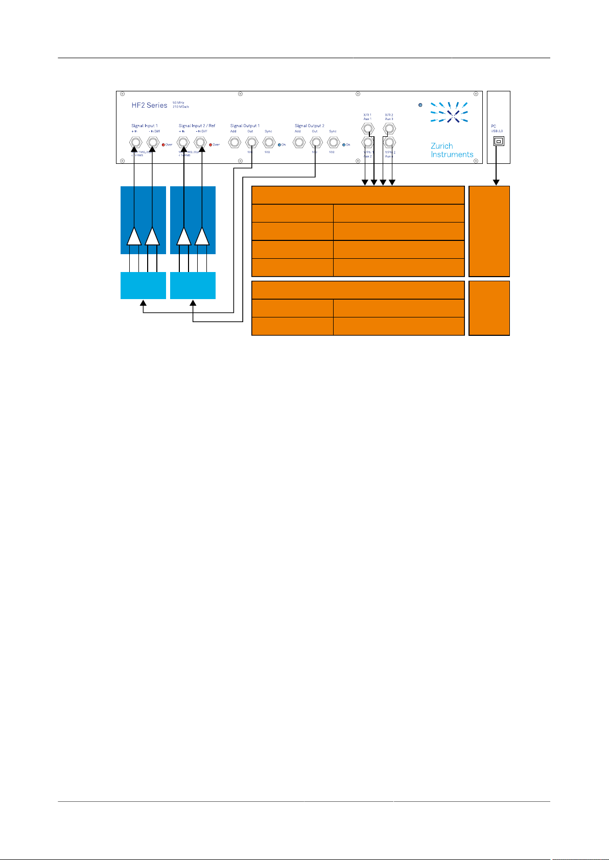
2.5. Operating Modes

DUT 1

HF2CA

drive signal 1

DUT 2

drive signal 2

HF2IS sample output (any 2 of)

Input 1&2

Input 1&2 MF

F1, F2, F3, F4

F1, F2, F3, F4, F5, F6, F7, F8

HF2LI sample output (any 2 of)

Input 1

Input 1 with MF

F1, H1a, H1b

F1, H1a, H1b, H1c, H1d, H1e

Input 2

Input 2 with MF

F2, H2a, H2b

F2, H2a, H2b, H2c, H2d, H2e

Max 6 sample streams

HF2LI

Max 8 sample streams

HF2IS

HF2CA

Figure2.6.HF2 internal reference mode / dual-channel

2.5.2.External Reference Mode

The external reference mode uses external reference sources to recover the signal of interest inside the HF2 Instrument. In this mode, the internal frequency generators are not used to stimulate the DUT. As the signal reference is an arbitrary periodic signal, a certain amount of time is required for the HF2LI to lock on the reference and to be able to recover the signal of interest reliably. This lock time depends on several parameters, but most important on the level and phase noise of the reference.

The external reference mode is supported with single-channel and dual-channel operation. This is possible as the HF2 Instruments includes 2 independent measurement units that are working autonomously. In single-channel mode, the reference can be fed into the Input 2/Ref connector on the front panel. This alternative provides an unmatched capability to use references with small amplitudes as they can be amplified by the signal path of Input 2. In dual-channel operation, the external TTL references are fed into the HF2 by means of the DIO0 and DIO1 connectors on the back panel.

HF2 User Manual - LabOne Edition Revision 34390 Zurich Instruments 42

Page 43

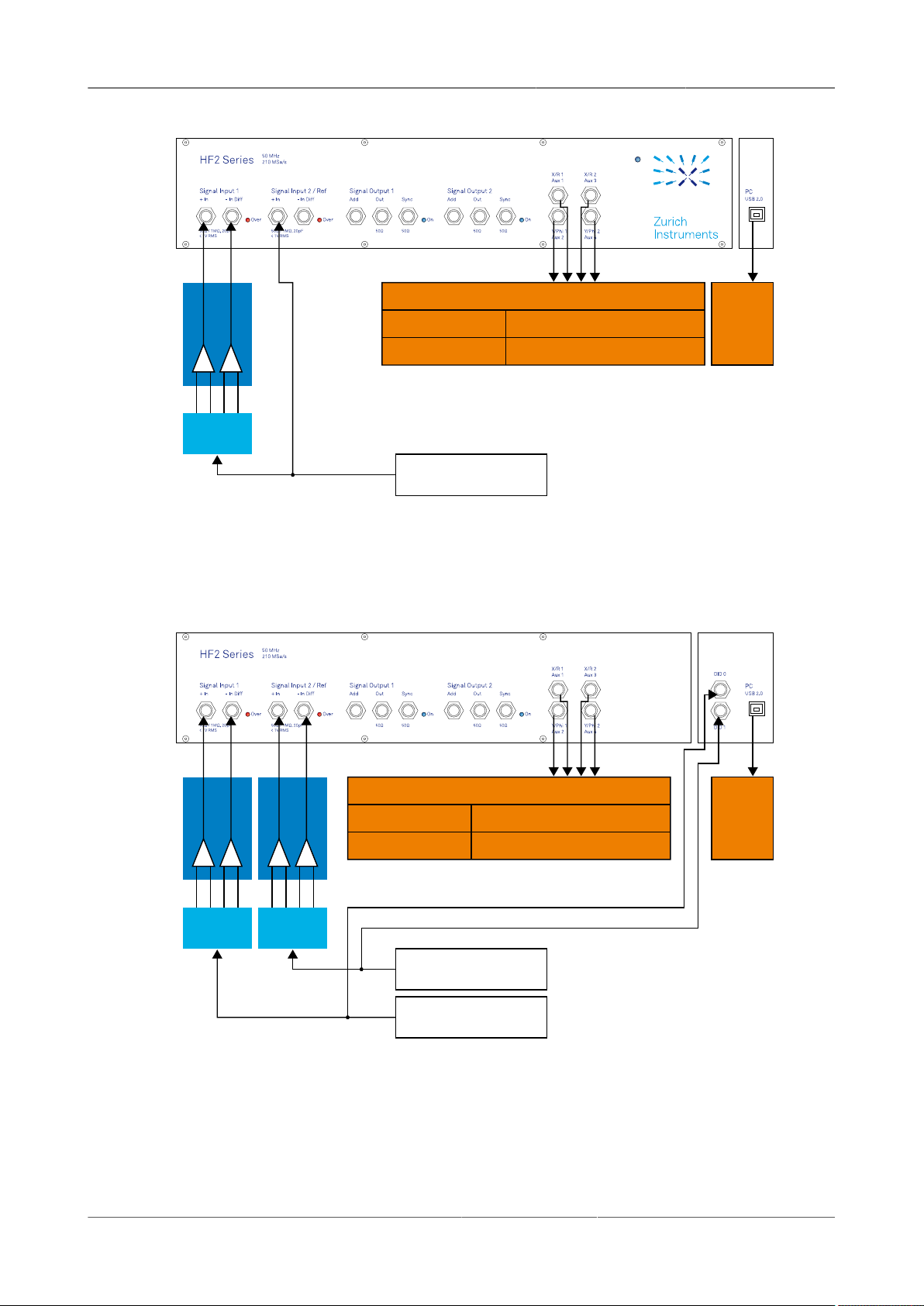
2.5. Operating Modes

DUT 1

External Generator 1

HF2CA

drive signal

HF2LI sample output (any 2 of)

Input 1

Input 1 with MF

F1, H1a, H1b

F1, H1a, H1b, H1c, H1d, H1e

Max 6 sample streams

HF2LI

reference

DUT 1

External Generator 2

HF2CA

reference 1

HF2LI sample output (any 2 of)

Input 1

Input 1 with MF

F1, H1a, H1b

F1, H1a, H1b, H1c, H1d, H1e

Max 6 sample streams

HF2LI

External Generator 1

DUT 2

reference 2

HF2CA

drive signal 1

drive signal 2

Figure2.7.HF2 external reference mode / single-channel

Figure2.8.HF2 external reference mode / dual-channel

2.5.3.Auto Reference Mode

HF2 User Manual - LabOne Edition Revision 34390 Zurich Instruments 43

Page 44

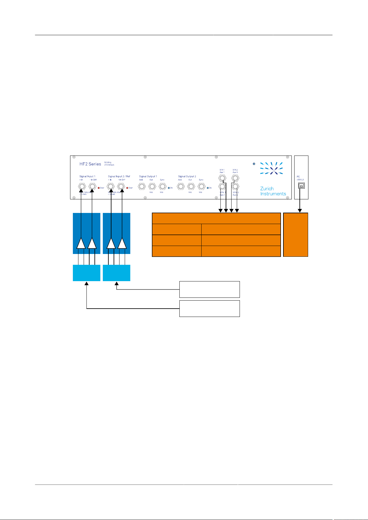
2.5. Operating Modes

DUT 1

Max 6 sample streams

HF2LI

HF2CA

drive signal 1

DUT 2

drive signal 2

External Generator 1

External Generator 2

HF2LI sample output (any 2 of)

Input 1

Input 1 with MF

F1, H1a, H1b

F1, H1a, H1b, H1c, H1d, H1e

Input 2 F2, H2a, H2b

HF2CA

The auto reference mode makes use of the internal PLLs to recover the reference frequency directly from the signal coming from the DUT. In this mode, the internal frequency generators are not used to stimulate the DUT. As the reference is inherently contained in the sampled signal, a dedicated PLL is able to lock on the frequency and to recover the reference and the signal of interest. This process is suited for signals with enough amplitude and signal-to-noise ratio. Further the reference recovery requires a certain amount of time that depends on several parameters like the level and the phase noise of the measured signal.

The auto reference mode is supported with single-channel and dual-channel operation. This is possible as the HF2 Instrument includes 2 independent measurement units that are working autonomously. In dual-channel mode it is sufficient to connect the signals captures at the DUTs to the Input 1 and Input 2 connectors of the HF2 Instrument. The HF2 Series support both singleended and differential input signals ideal for fixed and floating ground applications.

Figure2.9.HF2 auto reference mode / dual-channel

2.5.4.Multi-frequency Operation

The multi-frequency operation is the powerful extension provided by the HF2 Series increasing the number of frequencies that can be analyzed in parallel. Moreover, the multi-frequency considerably expands the multiplexing options the user has with respect of input channels and demodulator clocks. Please note that the HF2IS-MF is different than the HF2LI-MF (see Table2.4) as different features and different number of demodulators are activated.

For the HF2LI the multi-harmonic mode and the arbitrary frequency mode are distinguished. In multi-harmonic mode it is possible to analyze a signal at the fundamental frequency and at 5 harmonics at the same time, and the arbitrary frequency mode is the extension to analyze a signal of interest at 6 completely independent frequencies.

For the HF2IS only the arbitrary frequency mode is relevant.

HF2 User Manual - LabOne Edition Revision 34390 Zurich Instruments 44

Page 45

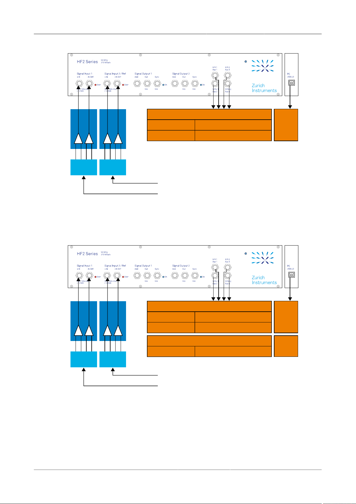
2.5. Operating Modes

DUT 1

HF2CA

drive signal 2

HF2LI sample output (any 2 of)

Input 1 with MF F1, H1a, H1b, H1c, H1d, H1e

Input 2 with MF F2, H2a, H2b, H2c, H2d, H2e

DUT 2

drive signal 1

Max 6 sample streams

HF2LI

HF2CA

DUT 1

drive signal 2

DUT 2

HF2CA

drive signal 1

Max 6 sample streams

HF2LI

HF2LI sample output (any 2 of)

Input 1 with MF F1, F2, F3, F4, F5, F6

Input 2 with MF

F1, F2, F3, F4, F5, F6

HF2IS sample output (any 2 of)

Input 1&2 MF F1, F2, F3, F4, F5, F6, F7, F8

Max 8

HF2IS

HF2CA

Figure2.10.HF2 multi-harmonic mode

Figure2.11.HF2 arbitrary frequency mode

HF2 User Manual - LabOne Edition Revision 34390 Zurich Instruments 45

Page 46

Chapter3.Tutorials

The tutorials in this chapter aim to help users perform their initial measurements with HF2 lock-in amplifiers using the LabOne User Interface. The tutorials require some basic laboratory equipment and equipment handling knowledge. For the tutorials, you'll need the following material:

• 1 USB 2.0 cable (supplied with your HF2 Instrument)

• 3 BNC cables (2 optional)

• 1 male shorting cap (optional)

• 1 oscilloscope (optional)

• 1 T-piece (optional)

Note

For all tutorials, you must have the LabOne software package installed as described in the Getting

Started Chapter. Start up the user interface as described in Section1.5.

HF2 User Manual - LabOne Edition Revision 34390 Zurich Instruments 46

Page 47

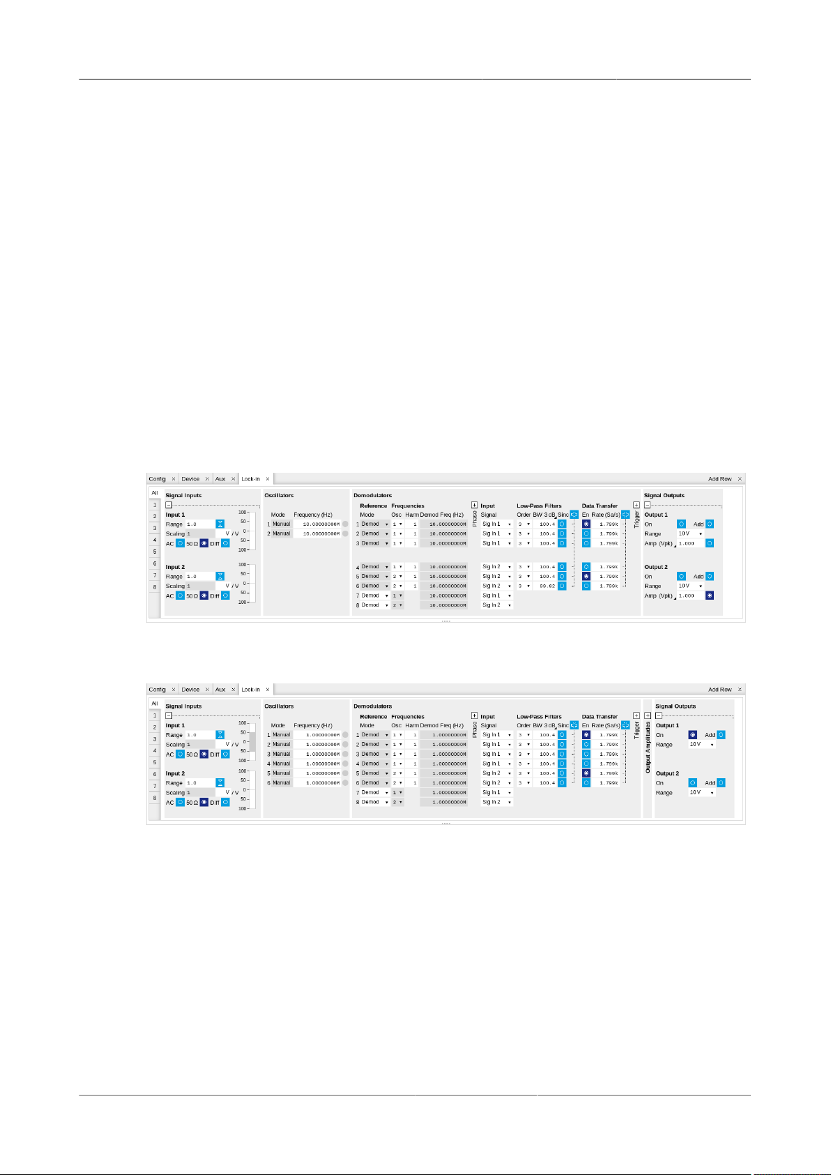
3.1. Tutorial HF2LI First Time User

3.1.Tutorial HF2LI First Time User

This tutorial covers basic operation of the HF2LI lock-in amplifier with the LabOne User Interface.

The LabOne User Interface is provided as the primary interface to the HF2LI but it is not the only program that can run the instrument. Typically, the user will use the LabOne UI to set up the instrument and then either use the LabOne UI to take the measurements or run (possibly concurrently) some custom programs.

Note

This tutorial aims to give a walk-through of the main features of the LabOne User Interface. Please also see Section4.1 for an overview of UI's layout and Chapter4 in general for a thorough description of all the available settings available in the LabOne UI for your instrument.

3.1.1.The Lock-in Tab

Figure3.1.The Lock-in tab

Figure3.2.The Lock-in MF tab

Open the Lock-in tab by clicking on the Lock-in icon on the left side of the user interface. If you find the Lock-in MF tab, it means that the instrument has the HF2-MF option installed. Section4.2 provides the full documentation of the Lock-in tab while Section4.3 describes the Lock-in MF tab.

The Signal Inputs section contains a Range that can be set to a value between 1 mV and 1.6 V, the largest amplification of the input signal is achieved for 1 mV. The input has protection diodes that clip signals with amplitude above 5 V.

HF2 User Manual - LabOne Edition Revision 34390 Zurich Instruments 47

Page 48

3.1. Tutorial HF2LI First Time User

Important

Please respect the compliance to the maximum ratings Table 8.2 to prevent damage to the instrument.

The AC button sets the coupling type: AC coupling has a cutoff frequency of 1 kHz. The AC coupling consists of a blocking capacitor between two input amplifier stages: this means that a DC signal larger than 5 V will saturate the front amplifier even if AC coupling is enabled. The Diff button sets single-ended/differential measurement mode: in the differential mode, the voltage difference between the +In and -In is amplified whereas in single-ended mode, the voltage at the +In connector is amplified. The 50 Ω button toggles the input impedance between low (50 Ω) and high (approx 1 MΩ) input impedance. 50 Ω input impedance should be selected for signal frequencies above 10 MHz to avoid artifacts generated by multiple signal reflections within the cable. With 50 Ω input impedance, one will expect a reduction of a factor of 2 in the measured signal if the signal source also has an output impedance of 50 Ω.

Next, one finds the Oscillators section used to control the frequency for the demodulation with an internal reference. For the purpose of this tutorial, set the frequency of oscillator 1 to 1 MHz.

Under the section Demodulators the user can select which harmonics and filter bandwidths to use for demodulation. It is not uncommon to need to measure different harmonics (integer multiples of the fundamental frequency, in this case 1 MHz). Select the harmonic (Harm) to 1 for the first demodulator (the first line), set the filter order to 4 (this corresponds to a filter steepness of 24 dB/ oct or 80 dB/dec, an attenuation of 104 for a tenfold frequency increase) and type 10 Hz into the BW control (the digital filters of the HF2 are described in Section9.3). Users are sometimes interested in the second harmonic that may be generated by nonlinear processes in their device under test: select harmonic 2 for the second demodulator and type the same values for the filter order and BW as in the previous case. You can also measure the same fundamental harmonic with a larger bandwidth: set harmonic to 1, order to 24 dB/oct and BW to 1 kHz for the third demodulator. Measuring with different bandwidths can provide the signal average and transient values. Click on the enable button next to the filters to read out the values from the 3 demodulators.

Next, set the Trigger to Continuous and the Rate to 7.20 kSa/s (rate settings can only be submultiples of 460 kSa/s, the maximum readout rate for one demodulator): in this case, the HF2LI will send the demodulated signal sampled at this rate through the USB. Due to the finite bandwidth of the USB connection the maximum cumulative demodulator sample rate is 700 kSa/s, which can be split over the active demodulators, see Table 8.4. In this example we're using 3 active demodulators, therefore, since the sample rates are sub-multiples of 460 kSa/ s the maximum possible readout rate for each demodulator is 230 kSa/s. Note that, according to the Nyquist sampling theorem , the sampling rate should be at least twice as fast as the maximum frequency present in the signal, in order to reconstruct the demodulated signal (this is not important if you only need one data point or the standard deviation of the demodulated signal). Since the low-pass filters do not have an infinite roll-off (the attenuation is not infinite past the filters' 3 dB frequency), it is common to set the sampling rate to about 8 times higher than the filter bandwidth.

Next, we configure the HF2 to output a 1 MHz signal on its Signal Output 1/Out connector. In case you have the HF2-MF Option installed, go to the Signal Outputs section, set the excitation amplitude Amp (Vpk) to 100 mV and the output range to be the smallest possible but at least twice as large as than the amplitude for minimum harmonic distortion. Connect Signal Output 1 to Signal Input 1 +In with a BNC cable and click on the On button in the LabOne Signal Outputs section of Output 1. With the HF2-MF Option installed, first go the Output Amplitudes section, set the signal amplitude Amp 1 (Vpk) of demodulator 7 to 100 mV and enable the button next to the amplitude field. Connect Signal Output 1 to Signal Input 1 +In with a BNC cable and click on the On button in the LabOne Signal Outputs section of Output 1.

HF2 User Manual - LabOne Edition Revision 34390 Zurich Instruments 48

Page 49

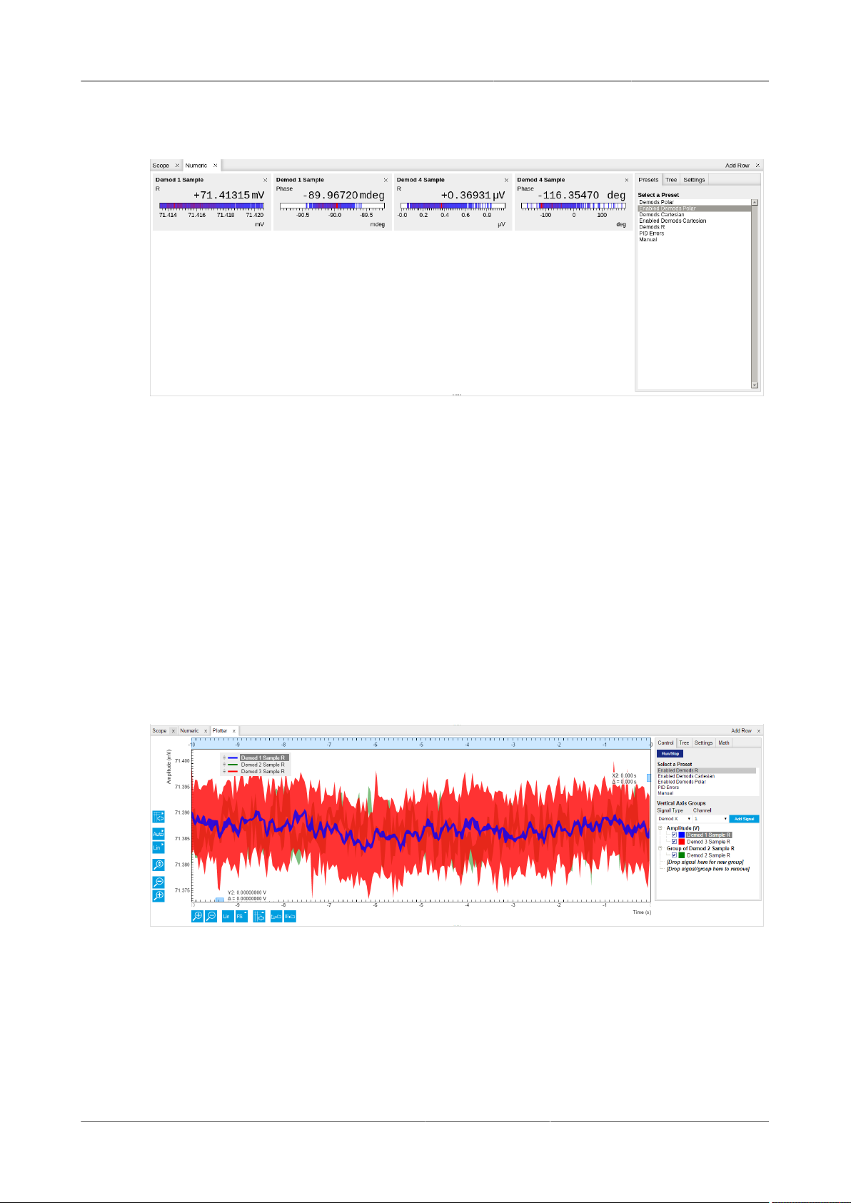
3.1. Tutorial HF2LI First Time User

3.1.2.The Numeric Tab

Figure3.3.The Numerical tab

In the Numeric tab, you should read 71 mV RMS for the R component of demodulator 1, (demodulating at 1 MHz). The RMS corresponds to the 100 mV divided by √2. The phase value will depend on the BNC cable length (for lengths shorter than one meter, the phase is approximately a few degrees). Demodulator 3 (also at 1 MHz) will show the same amplitude, but the digits fluctuate more, since the measurement bandwidth and therefore the noise, is larger. Demodulator 2 reads only a few μV because at 2 MHz (the second harmonic) there is only a little component of the signal, coming from the harmonic distortion of the HF2LI output and input stages.

3.1.3.The Plotter Tab

Figure3.4.The Plotter tab

Now open the Plotter tab. Here one can display the demodulated values over time. Select Enabled Demods R from the Presets and click on Run/Stop to start the acquisition. The demodulated traces for these three demodulators are displayed, offset to one another: as before, demodulators 1 and 3 have the same average value, but a larger noise amplitude is clearly visible in the third trace. In Section4.1.3 you can find a detailed description of the functions of the plot window. For instance you can find there ways to change the horizontal and vertical scales, to remove offsets

HF2 User Manual - LabOne Edition Revision 34390 Zurich Instruments 49

Page 50

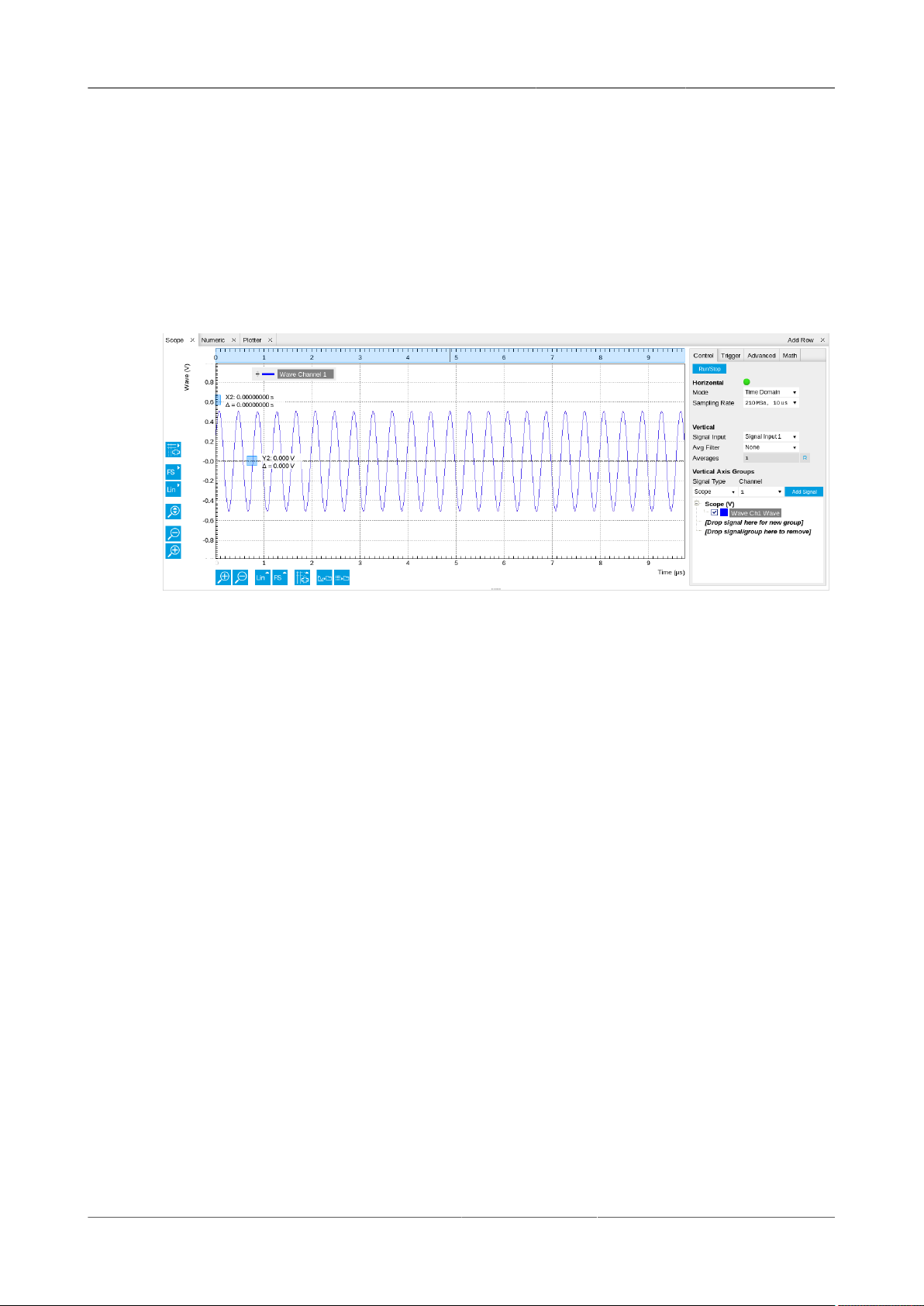
3.1. Tutorial HF2LI First Time User

in the plot, and to use the cursors for exact measurements. The amount of stored data depends on the set Window Length in the Settings sub-tab.

3.1.4.The Scope Tab

Figure3.5.The Scope

Let us proceed to the Scope tab. The Scope can be used to display the signal at the signal inputs and outputs of the HF2LI. It has a 2048 point wave memory that is useful for visualizing the raw signal. It also replaces the need for an external oscilloscope. Select Signal Input 1 in the Vertical section of the Control sub-tab, Signal Output 1 as the Signal in the Trigger sub-tab and press the Run/Stop button. The 1 MHz input signal is visible as 10 full cycles if the Sampling Rate is set to 210 MS, 10 μs in the Control sub-tab. Decreasing the sampling rate to display a longer time interval should be done carefully because it may lead to aliasing: for instance setting the sampling rate to 26 kSa/s, 80 ms, will produce a correctly looking sinusoidal, but at the wrong frequency. The BW Limit button in the Advanced sub-tab may reduce aliasing effects without removing them completely.

The update rate of the oscilloscope frames is controlled by the Holdoff time in the Trigger subtab: the minimum interval between two traces is 10 ms. This is a low value which increases the load of the USB bandwidth and may lead to USB sample loss - therefore avoid using small hold off values if not needed.

You can go from the time domain display to a frequency domain display by selecting the Freq Domain FFT Mode in the Control sub-tab. The frequency resolution is coarse because the time trace contains 2048 points. Averaging of the Fourier power spectra can be enabled to increase the SNR ratio.

3.1.5.The Sweeper Tool

HF2 User Manual - LabOne Edition Revision 34390 Zurich Instruments 50

Page 51

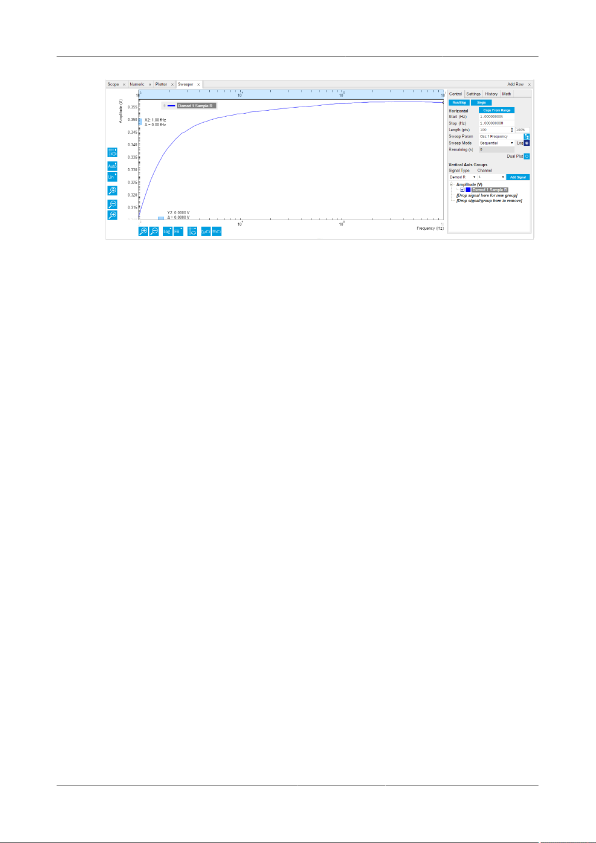
3.1. Tutorial HF2LI First Time User

Figure3.6.The Sweeper

Next is the Sweeper tool: it turns the HF2LI into a frequency response analyzer, giving the transfer function of a device under test in the form of a Bode plot. In AFM applications this is useful to easily identify the resonance frequency of a cantilever as well as the phase delay. The sweeper tool can also be used to sweep parameters other than frequency: phase, time constant, amplitude and auxiliary output voltage.

As a frequency sweeper example, we will execute a logarithmic sweep of 100 points between 1 kHz and 1 MHz. In the Horizontal section, set the sweep range Start to 1 kHz and Stop to 1 MHz, 100 points and enable the Log Sweep. Click on Run/Stop for continuous sweeping or on Single for a single sweep. Toggle the AC input coupling in the Lock-in settings, and observe the attenuation in the response at 1 kHz in AC coupling, since the AC coupling has a cutoff frequency of approximately 1 kHz. In the History sub-tab, the measurement that is displayed can be saved to a data file in ASCII format. There it is also possible to declare one out of several measured traces as a reference by selecting the trace in the list and clicking on Reference. The selected trace then appears below the list, and next to it there is the enable button for the reference mode. In reference mode, all traces in the plot are divided by the reference trace.

During the logarithmic sweep the NEPBW (noise equivalent power bandwidth) is adjusted for each frequency point and displayed under the Filters BW field under the Lock-in tab. The adjustment is due to the fact that the sweep is logarithmic and the sweep frequency steps are not equally spaced. In order to account for all signal power (and power densities), the measurement bandwidth must be changed accordingly. This can be done automatically by going from Application Mode to Advanced mode in the Settings sub-tab, and there selecting Auto as the Bandwidth Mode. For an explanation of the NEPBW, see Signal Processing chapter. Note that in this configuration, if the signal to noise ratio is large, there will not be any effect when disabling Auto BW, since the noise signal is negligible when measured with (almost) any NEP bandwidth. Averaging can also help to improve the signal-to-noise ratio during the sweep.

As an example of noise measurement, disconnect the BNC cable from Signal Output 1 and connect it to Signal Output 2. In the Lock-in tab, turn off the Signal Output 1, and generate a 100 kHz / 100 mV excitation Signal Output 2 (remember to turn on the output in the Signal Outputs section). In the frequency sweeper perform a single sweep with Auto BW enabled. A relatively wide peak will appear at 100 kHz, as the measurement was performed with wide NEPBW. Switch the X scaling to Manual and zoom into the region around 100 kHz; click the Copy From Range button to use the new boundaries for the sweep as selected in the graph and again perform a single sweep. The peak at 100 kHz will appear narrow, reflecting the change in the measurement bandwidth.

3.1.6.The Spectrum Tab

HF2 User Manual - LabOne Edition Revision 34390 Zurich Instruments 51

Page 52

3.1. Tutorial HF2LI First Time User

Figure3.7.The Spectrum tab

The Spectrum tool (more information (see Section9.6) allows the user to measure the frequency spectrum around a specific frequency: this is done by performing the Fourier transform of the demodulated X and Y (or in-phase and quadrature) components of the signal (more precisely of the quantity X+jY, where j is the imaginary unit). This method is called zoomFFT. The frequency resolution that can be achieved in this way is given by the sampling rate divided by the number of recorded samples, and is therefore much higher than the frequency resolution obtained in the Scope tab. The zoomFFT approach is more efficient than the FFT on raw samples in which one digitizes a long time trace, performs the Fourier transform and retains only the portion of the frequency spectrum of interest while discarding the rest.

We continue from the previous section with the BNC connecting Signal Output 2 to Signal Input 1, and 100 mV, 100 kHz sine wave. In the Lock-in tab, set the oscillator 1 frequency to 101 kHz. Set the Demodulator 1 parameters to filter order 4, filter bandwidth 500 Hz, and Data transfer rate

7.2 kSa/s. In the Spectrum tab, enable Filter Compensation and select Demodulator 1 for Signal Input. A peak appears at 1 kHz to the left of the center frequency. Increasing the number of lines in FFT will result in a finer frequency resolution. The Filter compensation button compensates for the demodulator filter, by dividing the measured spectrum by the demodulator filter transfer function. This is why the input signal does not appear attenuated despite being outside the filter bandwidth (1 kHz and 500 Hz respectively).

3.1.7.The Auxiliary Tab

Figure3.8.The Auxiliary Tab

The Auxiliary tab controls the 4 Auxiliary Outputs on the right side of the HF2LI front panel, as well as the 2 Auxiliary Inputs on the rear panel. On the Aux Output section of the Auxiliary tab, output

HF2 User Manual - LabOne Edition Revision 34390 Zurich Instruments 52

Page 53

3.1. Tutorial HF2LI First Time User

the signal amplitude by selecting R from the Signal pull-down menu from Aux 1 and Demod 1 from Channel. Set the Scale factor to 10 V/V which corresponds to the amplitude of the signal as you can read it in the Numeric tab, multiplied by the scale factor. If one is interested in small variations of the signal amplitude, an offset can be applied to the output: type -0.712 in Offset (V) (or alternatively click the counter facing arrows next to Offset (V)): Value (V) should now read 0.

: you should read 0.712 V in the output Value (V) field,

RMS

HF2 User Manual - LabOne Edition Revision 34390 Zurich Instruments 53

Page 54

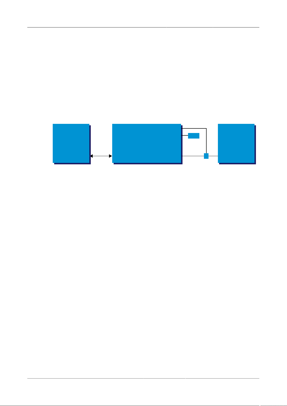
3.2. Tutorial Simple Loop

Oscilloscope

Channel 1

HF2 Series Input 1+

Input 1-

Output 1

Host Computer

USB 2.0

Cap

USB 2.0

3.2.Tutorial Simple Loop

3.2.1.Preparation

In this tutorial you generate a signal with the HF2 Instrument and measure that generated signal with the same Instrument. This is done by connecting Signal Output 1/Out with Signal Input 1/+In with a BNC cable. This tutorial shows a single-ended operation, meaning that there is no signal going into the Signal Input 1/-In connector. For proper operation, the Channel 1 must be set to single-ended operation, or alternatively the Input 1 - connector must be shorted to ground using a male shorting cap. Optionally it is possible to connect the generated signal at Output 1 to an oscilloscope by using a T-piece and an additional BNC cable.

Figure3.9.Tutorial simple loop setup

Note

This tutorial is both for HF2LI Lock-in Amplifier and HF2IS Impedance Spectroscope users.

Connect the cables as described above. Make sure the HF2 unit is powered on, and then connect the HF2 to your computer with a USB 2.0 cable. Finally launch LabOne (Start Menu/Programs/ Zurich Instruments/LabOne User Interface HF2).

3.2.2.Generate the Test Signal

Apply the following settings in order to generate a 2.5 MHz signal of 0.5 V amplitude on Signal Output 1/Out.

• Open the Lock-in tab and set frequency of Oscillator 1 to 2.5 MHz: click on the field, enter "2.5 M" or "2.5E6" and press <TAB> on your keyboard to confirm the data

• In the Output 1 section, set the Range pull-down of 1 V

• Without HF2-MF option: In the Output 1 section, set the amplitude to 0.5 V by entering 0.5

followed by a <TAB>

• With HF2-MF option: In the Output Amplitudes section, set Amp 1 (Vpk) of demodulator 7 to

0.5 V by entering 0.5 followed by a <TAB>.

• By default all physical outputs of the HF2 are inactive to prevent damage to connected circuits. Now turn on the main output switch by clicking on the button labeled "On".

HF2 User Manual - LabOne Edition Revision 34390 Zurich Instruments 54

Page 55

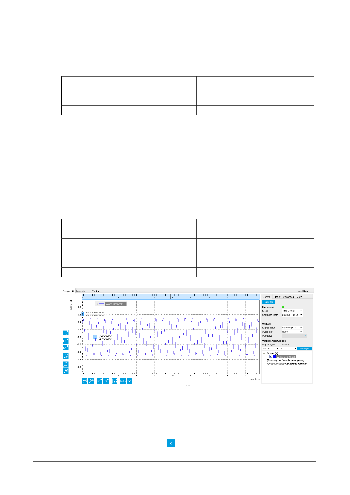
3.2. Tutorial Simple Loop

• If you have an oscilloscope connected to the setup, you are able to see your generated signal

Table3.1.Settings: generate the test signal

Output 1 range 1 V Oscillator 1 Frequency 2.5 MHz Demodulator 7 Amp 1 0.5 V Output 1 ON

3.2.3.Acquire the Test Signal

Next, you adjust the input parameters in order to acquire signals with the appropriate input range. To do this, you switch the signal source and the trigger of the Scope to Signal Input 1. Then you adjust the Signal Input 1 range to 1 V.

Table3.2.Settings: acquire the test signal

Scope Signal Input Signal Input 1 Scope Trigger Signal Signal Input 1 Scope Sampling Rate 210 MS, 10 us Run / Stop RUN Signal Input 1 range 1 V Signal Input 1 AC / 50 / Diff ON / OFF / OFF

Figure3.10.LabOne UI displaying the acquired signal

The Scope displays the measured signal at Input 1. Having set the input range to 1 V ensures that no signal clipping occurs. If you try and set the input range to 0.3 V you see the effect in the Scope window. Note how the red "Over" LEDs on the front panel of the HF2 indicates the error condition and the set OV (OVI) status flag on the right-bottom corner of the window. Set back the input range

to 1 V and then clear the flag by clicking .

HF2 User Manual - LabOne Edition Revision 34390 Zurich Instruments 55

Page 56

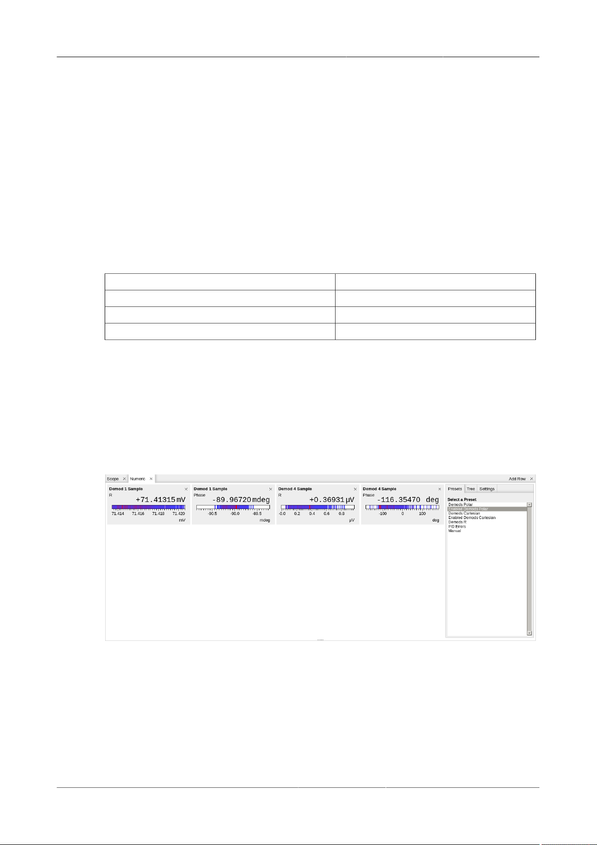
3.2. Tutorial Simple Loop

The Scope is a very handy tool to quickly check settings before proceeding to more advanced measurements, please refer to Section4.6 for a full description of features available in the Scope.

3.2.4.Measure the Test Signal

Next you use the demodulators of the HF2 to measure acquired test signal. You will use the Numeric and the Plotter tab from the LabOne user interface. First apply the following settings (choose any of the demodulators 1 to 6).

Table3.3.Settings: measure the test signal

Filter BW 3 dB 7 Hz (approximated to 6.8 Hz) Filter order 2 Data transfer rate 100 Hz (approximated to 112 Hz) Data transfer enable (En) ON

These settings set the demodulation filter to second-order low-pass operation with a 7 Hz bandwidth. The corresponding time constant can be obtained easily by clicking on the label on top of the bandwidth setting column according to Equation9.3 provided in Chapter9. The output of the demodulator filter is read out with 100 Hz, implying that 100 data samples are sent to the host PC per second. These samples are viewed in the Numeric and Plotter tab that we examine next.

The Numeric tool provides the space for 6 measurement panels corresponding to the 6 demodulators. Each of the panels has the option to display the samples in Cartesian (X,Y) or polar format (R,Θ) . The unit of the (X,Y,R) values is V

RMS

Figure3.11.LabOne UI Numeric tab

If you wish to play around with the settings, you could now change the amplitude of the generated signal, and observe the effect on the demodulator output.

Next, we'll have a look at the tab. This tab provides a time plot of the demodulator outputs. It is possible to plot up to 6 signals continuously as (X,Y) or (R,Θ) pairs, to set different scales, or to make detailed measurements with 2 cursors. For a detailed description of the functionality available in the Plotter please see Section4.5 and Section4.1.3.

HF2 User Manual - LabOne Edition Revision 34390 Zurich Instruments 56

Page 57

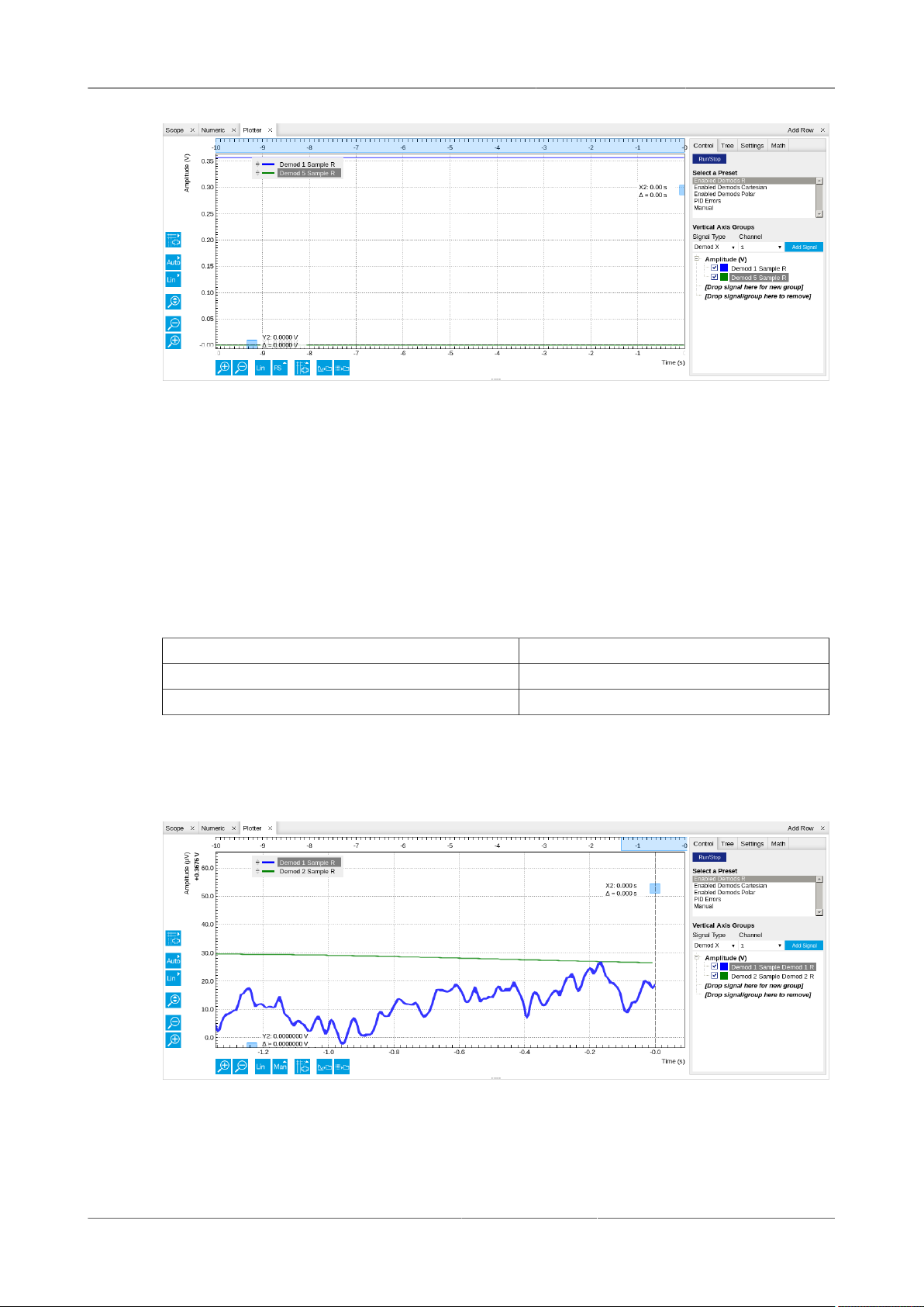
3.2. Tutorial Simple Loop

Figure3.12.LabOne Plotter view with plot of demodulator 1 output (TC = 10 ms)

3.2.5.Different Filter Settings

As last step of this tutorial you change the filter settings and see the effect on the measurement results. For instance you change the time constant of the integration to 2 seconds.

Table3.4.Settings: changing the filter settings

Time constant (TC) 2 s Filter slope 12 dB/Oct Resulting measurement bandwidth (BW) ~51 mHz

Increasing the time constant increases the integration time of the demodulators smoothing out the demodulator outputs. This averages the noise over time and the output of the filters is more stable. This manifests itself in a smoother curve of the demodulator data but also in a larger number of stable digits in the Numeric tab.

Figure 3.13. LabOne Plotter displaying the data of two demodulators with different time constants

HF2 User Manual - LabOne Edition Revision 34390 Zurich Instruments 57

Page 58

3.3. Tutorial Dynamic Signals

Oscilloscope

Channel 1

HF2 Series Input 1+

Input 1-

Output 1

Add 1

Output 2

Host Computer

USB 2.0

3.3.Tutorial Dynamic Signals

3.3.1.Preparation

In this tutorial we generate a test signal of 2.5 MHz with an amplitude modulated at a frequency of 1 Hz. Then we measure the test signal using two different filter settings.

Figure3.14.Tutorial dynamic signals setup

Note

This tutorial can be performed both on the HF2LI Lock-in Amplifier and on the HF2IS Impedance Spectroscope and will use the Input connector. The generation of multi-frequency signals is simple on the HF2LI with the HF2-MF option or on the HF2IS, where there is no need to make use of the ADD connector.

3.3.2.Generate the Test Signal

In this section you generate a 2.5 MHz sinusoidal signal whose amplitude oscillates at 1 Hz. This is also called the beat signal. In order to obtain this test signal you add two sinusoids of the same amplitude but with a 1 Hz difference in the frequency.

Table3.5.Settings: generate the test signal

Output 1 range 1 V / ON Output 2 range 1 V / ON Oscillator 1 frequency 2'500'000 Hz Demodulator 7 Amp 1 0.3 V / ON Oscillator 2 frequency 2'500'001 Hz Demodulator 8 Amp 2 0.3 V / ON Signal Output 1 Add ON

When connecting an oscilloscope to the Output 1 connector, you should be able to observe the superposition of the 2 sinusoids. To see the acquired signal inside the LabOne User Interface switch to the Scope tab. The Scope view looks like this with the following settings.

HF2 User Manual - LabOne Edition Revision 34390 Zurich Instruments 58

Page 59

3.3. Tutorial Dynamic Signals

-0.00 0.05 0.10 0.15 0.20 0.25 0.30

-0.4

-0.2

0.0

0.2

0.4

Y1: 0.000 V

X1: 0.0000 s

Y2: 0.000 V Δ = 0.000 V

X2: 0.0000 s Δ = 0.0000 s

Table3.6.Settings: acquire the test signal

Scope Signal input Signal Input 1 Scope Trigger signal Signal Input 1 Scope sampling rate 6.4 kSa, 320 ms Run/Stop Run Signal Input 1 range 1 V Signal Input 1 AC / 50 / Diff ON / OFF / OFF

0.00 0.05 0.10 0.15 0.20 0.25 0.30

Wave (V)

Wave Channel 1

Figure3.15.LabOne UI displaying the acquired signal

The beat signal has a maximum amplitude of 0.6 V, thus it falls within the set range of 1 V. The range setting will prevent any higher voltage than what is set - even if 2 sinusoidals of 0.7 V amplitude each would be added like done in this section, the output would be clipping at 1 V which is the set range. Try to change the output range to 0.1 V, and see how the output voltage is changed to prevent inconsistent settings.

3.3.3.Measure the Test Signal

First you change to the Plotter tab, set the scale in order to view an interesting set of data, and set the demodulator filters to a low time constant to measure the amplitude of the 2.5 MHz signal (Hull curve).

Table3.7.Settings: filter with a low time constant

Time constant (TC) 10 ms (approximated to 10.2 ms) Filter order 2 Resulting measurement bandwidth (BW 3dB) ~10 Hz Data transfer rate 100 Hz (approximated to 112 Hz) Data transfer enable (En) ON

These settings set the demodulation low-pass filter to a 10 ms time constant (the corresponding bandwidth is around 10 Hz) and the filter slope to second order. The output of the filter is sampled at a rate of 100 Hz, and the samples are sent to the host computer.

Time (s)

HF2 User Manual - LabOne Edition Revision 34390 Zurich Instruments 59

Page 60

3.3. Tutorial Dynamic Signals

-0.00

0.05

0.10

0.15

0.20

0.25

0.30

0.35

0.40

Y1: 3 mV

X1: -5.162 s

Y2: 0.424 V Δ = 0.421 V

X2: -6.144 s Δ = -0.982 s

-10 -9 -8 -7 -6 -5 -4 -3 -2 -1 -0

Amplitude (V)

Figure3.16.LabOne UI displaying the measured signal

If you stop the acquisition by pressing the button "Run/Stop" you can conveniently measure the amplitude of the 1 Hz signal by using the 2 cursors C1 and C2: 394.4 mV You can achieve higher measurement precision by using a even lower time constant (e.g. 1 ms), increasing the readout rate (e.g. 1.8 kHz), and zooming into the Plotter view.

Demod 1 Sample R

Demod 1 Sample Phase

, half period 498.1 ms.

RMS

Time (s)

Next you use a high time constant to separate the 2 original sinusoids even though they are superposed in one signal. In the Lock-in tab apply the following settings.

Table3.8.Settings: filter with a high time constant

Time constant (TC) 2 s Filter order 2 Resulting measurement bandwidth (BW 3dB) ~35 mHz Data transfer rate 100 Hz (approximated to 112 Hz) Data transfer enable (En) ON

These settings set the demodulation low-pass filter to a time constant of 2 s, with a resulting measurement bandwidth of 35 mHz. With these settings the HF2 is able to distinguish between the signal component at 2'500'000 Hz and the signal component at 2'500'001 Hz as the measurement bandwidth is considerably less than the frequency spacing of the 2 signal components. The output of the demodulator is stable after a settling time.

HF2 User Manual - LabOne Edition Revision 34390 Zurich Instruments 60

Page 61

3.3. Tutorial Dynamic Signals

0.2125

0.2130

0.2135

0.2140

0.2145

0.2150

0.2155

Y1: 0.000000 V

X1: 0.00 s

Y2: 0.214058 V Δ = 0.214058 V

X2: 0.00 s Δ = 0.00 s

-10 -8 -6 -4 -2 -0

Amplitude (V)

Figure3.17.LabOne UI displaying the measured signal

Demod 1 Sample R

Time (s)

The output of the demodulator does not show any oscillations like before: the numerical value is mV

. If you switch to the oscilloscope view, you see that the signal at Input 1 is still beating

RMS

as before, while the demodulator filter is set such to ignore the interferer at 2'500'001 Hz. Try to switch off the interferer.

Table3.9.Settings: remove the interferer

Signal output 2 ON/OFF OFF

The time it takes to settle depends on various parameters like filter setting and switch-off timing. The difference in amplitude of the measurement at 2'500'000 Hz with or without interferer is in the range of 50 μV. With different filter settings it is possible to do better than that.

Consider this: you have 2 signals with relevant amplitude (0.3 V) interfering with each other as their frequency is very close (1 Hz at 2.5 MHz). The power of lock-in amplification consists of extracting the relevant signal energy at exactly one frequency. The "immunity" from nearby interferer is the capability to ignore them. This a simple definition of the dynamic reserve.

3.3.4.Filter Setting Discussion

This section aims to summarize a few basic concepts of filtering in connection with lock-in amplification. In this tutorial, you have used different filter settings to measure different signal properties.

HF2 User Manual - LabOne Edition Revision 34390 Zurich Instruments 61

Page 62

3.3. Tutorial Dynamic Signals

Table3.10.Settings: filter with a high time constant

Time constant Measurement

bandwidth

Low setting High, capability

to detect fast events

High setting Low, capability

to determine the steady state

Filtering constitutes a trade-off between measurement speed and measurement accuracy. In order to measure fast events, it is necessary to open up the filters allowing also more noise in the measurement result. The opposite is to measure with narrow filters which increases the signalto-noise ratio, but limits the capability to detect the changes in the signal of interest. This tradeoff is in common with any lock-in amplifier. The power of the HF2 is that it allows to do both at the same time thanks to the multiple demodulators per input channel.

Measurement noise

More noise in measurement result

Less noise in measurement result

Changes upon steady state change

Fast adaptation of result

Slow adaptation of result

Example

BW = 10 kHz, capability to detect events at 2-5 kHz, prone to pick-up noise

BW = 50 mHz, exact determination of steady state - events more frequent than 0.1 Hz are filtered

HF2 User Manual - LabOne Edition Revision 34390 Zurich Instruments 62

Page 63

3.4. Tutorial External Reference

Cap

Host Computer

USB 2.0

Cap

HF2 Series Input 1+

Input 1-

Output 1

Input 2+

Input 2-

Output 2

USB 2.0

3.4.Tutorial External Reference

3.4.1.Preparation

In this tutorial we generate a test signal with the HF2 and use it as a reference signal for demodulation in the same way as we would do it with a reference signal coming from an external source.

This is done by connecting the Output 2 connector with the Input 2+ connector with a BNC cable. This tutorial shows a single-ended operation, meaning that there is no signal going into the Input 2- connector. Optionally, it is possible to connect the generated signal from Output 2 to an oscilloscope by using a T-piece and an additional BNC cable. The Output 1 connector is to be connected to the Input 1+ connector. This allows you to check the generated reference signal. The measurement setup is shown in the following figure.

Figure3.18.Tutorial external reference setup

Make sure the HF2 unit is powered on, and then connect the HF2 to your computer with a USB 2.0 cable. Finally, launch LabOne (Start Menu/Programs/Zurich Instruments/LabOne User Interface HF2).

3.4.2.Generate the Reference Signal

In this section you generate a 1.0 MHz signal with a 1 V amplitude on Output 2 for use as the external reference. The settings for generating the reference signal are shown in the following table.

Table3.11.Settings: generate the reference signal

Output 2 range 1 V Demodulator 8 Amplitude 2 1.0 V / ON Oscillator 2 frequency 1 MHz Signal input 2 range / AC / Diff / 50 1.2 V / ON / OFF / OFF

When connecting an oscilloscope to the Output 2 connector, you should be able to observe the sinusoid. Alternatively, you can look at the signal in the LabOne UI Scope with the following settings.

HF2 User Manual - LabOne Edition Revision 34390 Zurich Instruments 63

Page 64

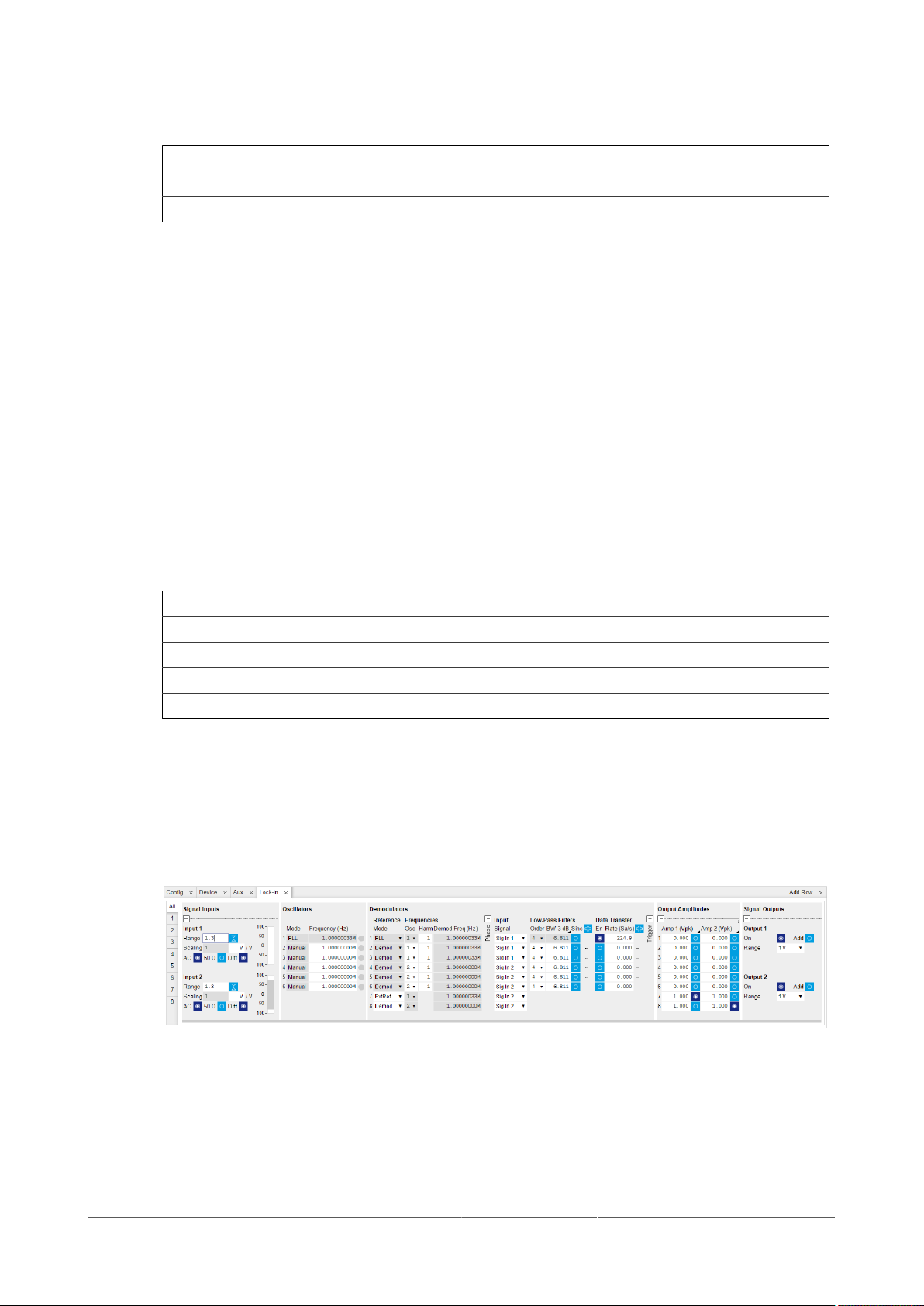
3.4. Tutorial External Reference

Table3.12.Settings: acquire the reference signal

Scope Signal Input Signal Input 2 Scope Trigger Signal Signal Input 2 Scope Sampling rate 53 MSa, 39 us

Note

In the Scope tab set the Horizontal Mode to Freq Domain FFT in order to see the frequency spectrum of the signal. This will also set a logarithmic Y scale by default. An Exponential Moving Average can be enabled in the Avg Filter field to reduce the noise floor in the display.

3.4.3.Activate the External Reference Mode

In this section we activate the external reference mode. Based on the external reference, we demodulate a separate signal of interest.

Table3.13.Settings: generate the signal of interest

Output 1 range 1 V Demodulator 7 Amp 1 1.0 V / ON Oscillator 1 frequency 1 MHz Demodulator 1 En/Rate ON / 100 Hz Signal Input 1 range / AC / 50 / Diff 1.3 V / ON / OFF / OFF

The external reference mode makes use of demodulators 7 and 8. These two demodulators can not be used for measurement. They serve as phase sensitive detectors to set up phase-locked loops locking an external reference and an internal oscillator. Demodulator 7 is assigned to oscillator 1, and demodulator 8 is assigned to oscillator 2. Previously we have chosen oscillator 2 as the source of the reference signal on Signal Output 2. Now we want lock oscillator 1 to this reference. In order to achieve that, we set the Mode field of demodulator 7 to ExtRef. In the pull-down selector in the Input column of demodulator 7, select Signal Input 2.

Figure3.19.LabOne UI enabling external reference mode

Once the external reference mode has been enabled, the frequency of oscillator 1 changes continuously, adapting to the frequency of the external reference signal. This can be verified by changing the frequency of oscillator 2 and noting how the frequency of oscillator 1 follows. A green light next to the oscillator frequency field indicates that the instrument has locked to an external reference.

HF2 User Manual - LabOne Edition Revision 34390 Zurich Instruments 64

Page 65

3.4. Tutorial External Reference

Host Computer

USB 2.0

Cap

HF2 Series Input 1+

Input 1-

Output 1

DIO 0

Aux Out 1

Output 2 ADD

Output 2

USB 2.0

In the demodulation process, the measurement signal is not multiplied directly with the external reference signal. Instead, the measurement signal is multiplied with newly generated reference signal from the internal oscillator, using only the frequency and phase information of the external reference. The continuous toggling of the oscillator frequency shows that the newly generated reference is continuously adjusted to the external reference.

3.4.4.Change External Reference Input

In this section you will modify the setup to use DIO 0 as the external reference instead of Signal Input 2. This is useful in practice since it means that the two sensitive Signal Inputs of the Instrument remain available for actual measurements. The modified setup is shown on

Figure3.20. Note that the DIO 0 connector is located on the back panel of the HF2 Instrument.

Figure3.20.Tutorial external reference using DIO 0 setup

It is important to make sure that DIO 0 is configured as an input before connecting anything to it. This can done using the DIO tab in LabOne. Note that the button to the right of bits 7...0 should be off.

When using the DIO 0 as the external reference signal, it should be taken into account that this is a digital I/O, which should be operated at TTL levels. Therefore the Aux 1 output is connected to the Add connector of Output 2, to provide a DC shift of the test signal and thus make it TTL compatible.

The settings used for generating the test signal are shown in the following tables. The resulting signal will have a DC offset of 1.5 V and an amplitude of 1 V and will thus oscillate between 0.5 V and 2.5 V, which is TTL compatible.

Table3.14.Settings: generate the test signal

Signal Output 1 range 1 V Signal Output 1 On / Add ON / ON Demodulator 8 Amp 2 1.0 V / ON Oscillator 2 Frequency 1 MHz

Table3.15.Settings: generate the DC shift

Aux 1 Signal Manual

HF2 User Manual - LabOne Edition Revision 34390 Zurich Instruments 65

Page 66

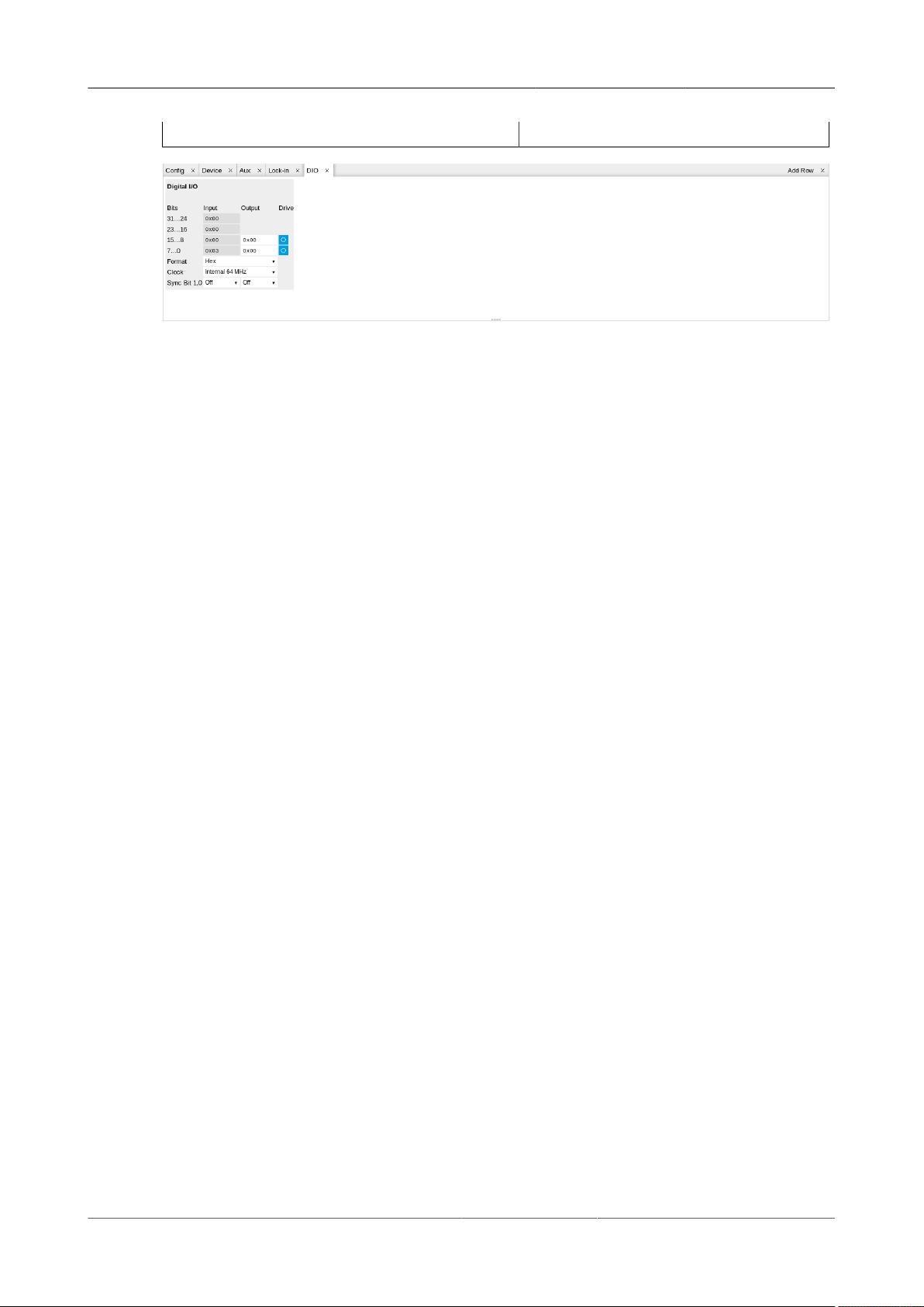
3.4. Tutorial External Reference

Aux 1 Offset 1.5 V

Figure3.21.Configuring DIO 0 as reference input

Finally use the Input pull-down selector for demodulator 7 in the Lock-in tab and set it to "DIO 0". This makes oscillator 1 lock on DIO 0. The frequency of oscillator 1 should start updating similarly to what was described in Section3.4.3.

HF2 User Manual - LabOne Edition Revision 34390 Zurich Instruments 66

Page 67

3.5. Tutorial Noise Measurement

3.5.Tutorial Noise Measurement

Lock-in amplifiers can be used to measure the noise on a signal. By quantifying the noise of a system one can estimate the maximum achievable performance.

3.5.1.How Does a Lock-in Measure Noise?

A lock-in amplifier measures the signal amplitude close to a given reference frequency with a defined bandwidth around this reference frequency. The noise in an input signal near the reference frequency appears as noise in the lock-in amplifier signal output.

The noise is the standard deviation of the measured X or Y value and is measured by first calculating the average, X from the X value to get the deviation. Finally, the RMS (root-mean-square) is calculated, corresponding to the total noise power of the input signal within a defined bandwidth around the reference frequency. The value is correct for input noise with Gaussian distribution of the noise power, which is normally the case.

Most of the times the noise spectral density is of interest, which is the normalization of the X

made independent of the filter bandwidth. To calculate the noise spectral density from the

noise

calculated RMS noise, one needs to divide the measured value by the square root of the bandwidth √BW. The noise spectral density has the units V/√Hz.

, over a defined period of time. Then, this signal, X

avg

, is subtracted

avg

The related equations are X The X and Y noise are expected to be identical.

= RMS(X - X

noise

)/√BW, and Y

avg

= RMS(Y - Y

noise

3.5.2.Measuring the Noise of the HF2LI/HF2IS

A LabVIEW example (ziExample-HF2-Noise.vi) is available to measure the noise in an input signal. To measure the equivalent input noise of the HF2, remove all BNC connectors from the input of the device and apply the following settings in the LabOne UI.

Table3.16.Settings: Measure HF2 Noise

Signal Input 1 range / AC / Diff / 50 0.01 V / ON / OFF / ON Demodulator 1 Low-Pass Filter BW 3dB = 100 Hz, Order = 4 Oscillator 1 Frequency 1 MHz Signal Output 1 switch OFF

Run the example, ziExample-HF2-Noise.vi. Make sure that the correct Demodulator is selected. The noise spectral density should now show a value close to 5 nV/√Hz. By changing the settings in the user interface, the noise behavior of the device can be analyzed in more detail. For example, changing the reference frequency to 10 kHz will slightly increase the spectral noise density, because of flicker noise that is larger at lower frequencies and generally present in all electronic circuits.

)/√BW respectively.

avg

HF2 User Manual - LabOne Edition Revision 34390 Zurich Instruments 67

Page 68

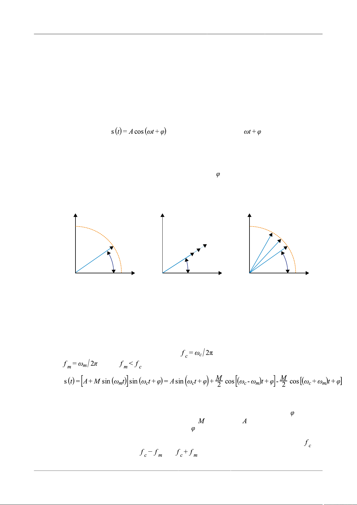
3.6. Tutorial Amplitude Modulation

(a) (b) (c)

amplitude

phase

3.6.Tutorial Amplitude Modulation

Note

This tutorial is addressed to HF2LI lock-in amplifier users that have purchased both HF2-MF multi-frequency and HF2-MOD AM/FM modulation options.

Amplitude modulation (AM) and frequency modulation (FM) refer to the modulation of an oscillating signal , the so-called carrier. A and are the amplitude and

the phase of the signal, respectively. Figure 3.22 depicts the phasor representation of s(t). The phasor follows a circle with radius A, and the phase wraps around after a full revolution of 360°. The signal s(t) is the projection of the phasor on the abscissa.

In the case of AM signals, the amplitude A, i.e. the phasor length, is time dependent, as in

Figure3.22(b). In the case of FM signals, the phase offset is time dependent and the phasor has

a constant amplitude, see Figure3.22(c).

Amplitude and frequency modulation, best known from radio transmission, are also common lock-in detection techniques.

Figure 3.22. A sinusoidal signal represented as a phasor: the signal corresponds to the projection on the x axis. Amplitude (b) and frequency (c) modulated signals affect the amplitude of the phasor or its phase

3.6.1.What is Amplitude Modulation?

In the time domain, amplitude modulation of the carrier signal produces a variation of the carrier amplitude proportional to the amplitude of the modulating signal. For example, when

the amplitude of a carrier with a frequency is modulated by a signal with frequency

(where ), the resulting signal has the form

Equation3.1.Amplitude modulation

where A and M are the amplitudes of the fast and slow modulations respectively and the phase offset. There is no restriction on the magnitude of compared to . The information of interest

is encoded in these three parameters, A, M and .

In the frequency domain, the AM signal s(t) is composed of three frequencies: the carrier at and two additional sidebands at and , as shown in Equation3.1. The two sidebands

HF2 User Manual - LabOne Edition Revision 34390 Zurich Instruments 68

Page 69

3.6. Tutorial Amplitude Modulation

time

freq

time domain

frequency domain

LI #1: first demod LI #2: second demod LI #3: carrier ampl

sideband fc-f

carrier f

fc-fm fc fc+fm

fc fm fc

TANDEM DEMODULATION

HF2LI with MOD OPTION

sideband fc+f

fc-fm fc+fm

have equal amplitude M/2, half of the modulating signal, and the carrier amplitude is independent on the modulation amplitude.

The traditional way of measuring an AM signal is called double (or tandem) demodulation and requires two lock-in amplifiers: the first one demodulates the signal at with a bandwidth that

is at least as large as (but smaller than ). This is to ensure that the full amplitude of the modulation signal is retained. The demodulated signal after the first lock-in becomes

Equation3.2.Tandem demodulation

In , the two sidebands are now located at the same frequency , while the carrier appears

as a DC component. When the demodulated signal is fed to a second lock-in amplifier, the result of the second demodulation at is proportional to .

In order to recover the amplitude it is necessary to measure the so one can divide the result by the factor . To measure the phase one can use a third lock-in to demodulate s(t) at the

carrier frequency with a bandwidth smaller than as shown in Figure3.23.

Instead of using a tandem configuration, the HF2-MOD option allows the user to demodulate directly at the three frequencies and simultaneously. The three parameters A, M and

can be measured and displayed with a single instrument.

Internally, the HF2LI generates the phases and from which it produces ,

and . This ensures the correct phase relationship for the demodulations of the

sidebands.

HF2 User Manual - LabOne Edition Revision 34390 Zurich Instruments 69

Figure 3.23. Comparison between tandem demodulation and the HF2-MOD option of an AM modulated signal

Page 70

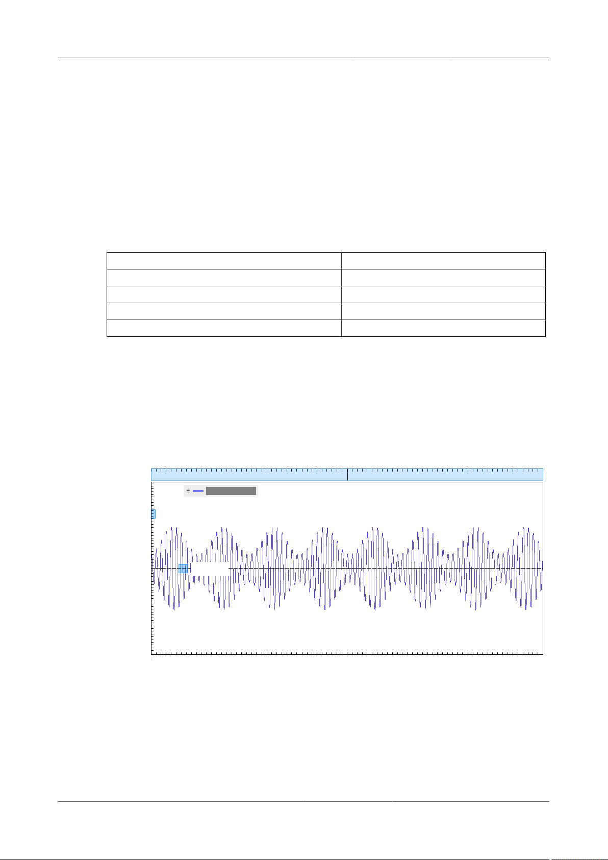
3.6. Tutorial Amplitude Modulation

-0.6

-0.4

-0.2

-0.0

0.2

0.4

0.6

Y1: 1 fV

X1: 0.00000000 s

Y2: 1 fV Δ = 0.000 V

X2: 0.00000000 s Δ = 0.00000000 s

3.6.2.Generate the Test Signal

In this tutorial, you are going to generate an AM signal with a carrier frequency of 1 MHz and a modulation frequency of 100 kHz. The signal is generated at Signal Output 2 and is demodulated by the first lock-in unit by feeding it into Signal Input 1. The HF2-MOD option requires the HF2MF Multi-frequency option because each modulated signal requires at least two oscillators. Note that changing the settings of Mod1 and Mod2 in the LabOne UI Modulation tab will modify some of the settings found in the Lock-in MF tab. The reader is kindly referred to Section4.18.

In the Modulation tab, in the Mod2 section, select the following parameters:

Table3.17.Settings: generate the AM signal

Carrier Oscillator (Osc)/Frequency Osc 1 / 1 MHz Sideband 1 Oscillator (Osc)/Frequency Osc 2 / 100 kHz Mode AM Carrier/Modulation 200 mV / 100 mV MOD 2 Enable ON

This generates an AM signal with the two sidebands of equal amplitude. To look at this signal, connect Signal Output 2 to Signal Input 1 of the HF2LI. Select the correct input parameters: in the Lock-in tab, for Signal Input 1, make sure Differential mode and 50 Ω are disabled. Then click on the auto range button (marked by A). In the Scope tab, select Source to be Signal Input 1, Trigger to be Signal Output 2 and click on Run to activate the scope. Observe how the carrier amplitude is modulated at 100 kHz. In Frequency Domain FFT mode, the plot shows three peaks: the carrier at 1 MHz and two sidebands at 0.9 and 1.1 MHz (see the cursors in the frequency domain representation in Figure3.25).

0 10 20 30 40 50 60 70

Wave (V)

Wave Channel 1

Figure3.24.Time domain representation of the AM signal generated by MOD2 measured with the LabOne Scope

HF2 User Manual - LabOne Edition Revision 34390 Zurich Instruments 70

Time (μs)

Page 71

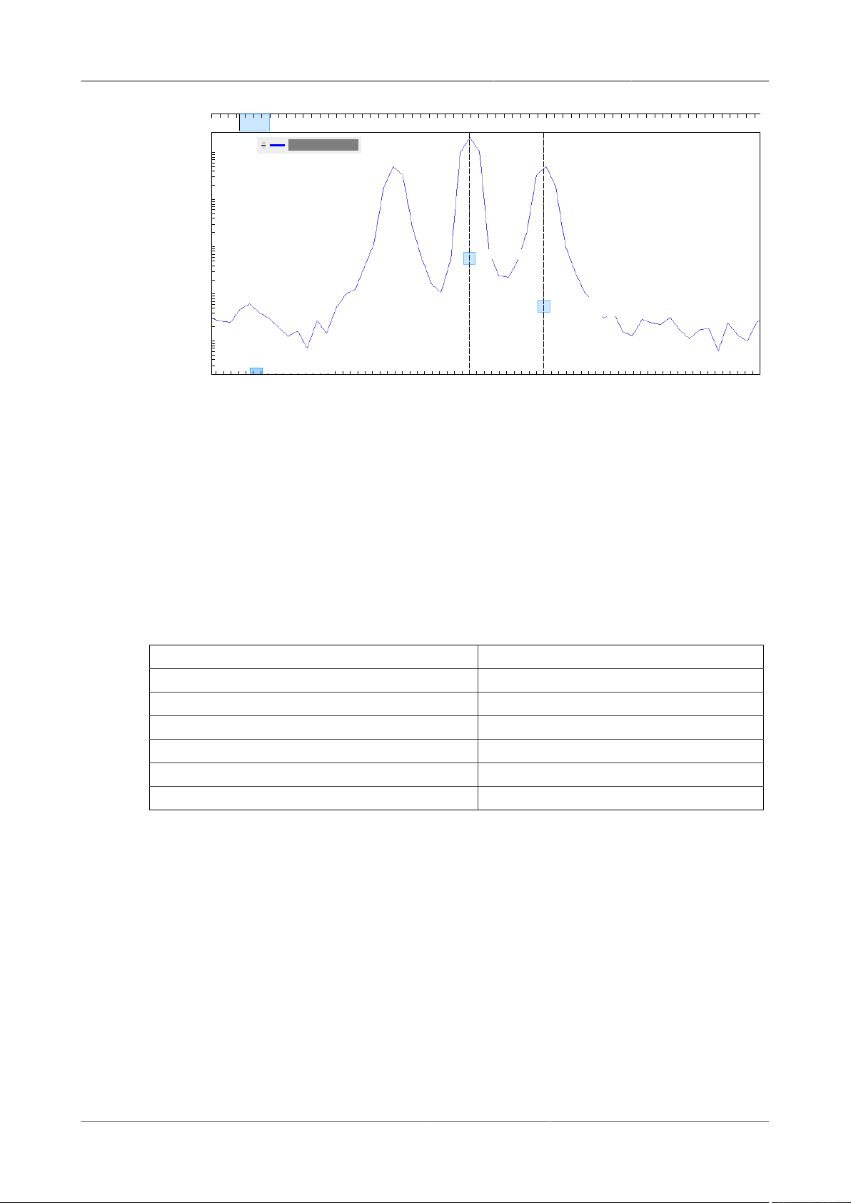
3.6. Tutorial Amplitude Modulation

700 800 900 1000 1100 1200 1300

-5

-4

-3

-2

-1

Y1: 1.0000 fV

X1: 1000.1 kHz

Y2: 1.0000 fV Δ = 0.0000 fV

X2: 1100.0 kHz Δ = 99.9 kHz

0 2 4 6 8 10 12

Wave (V)

Wave Channel 1

Figure3.25.Frequency domain representation of the AM signal generated by MOD2 measured with the LabOne Scope

Frequency (kHz)

3.6.3.Measure the Test Signal

In the Modulation tab, in the Mod1 section, select the following parameters:

Table3.18.Settings: measure the AM signal

Carrier oscillator (Osc) 1 Sideband 1 oscillator (Osc) 2 Mode AM Low-pass Filter BW (Carrier) 10 Hz Low-pass Filter BW (Sideband 1) 10 Hz MOD 1 Enable ON Demod 1, 2, 3 Data Transfer Enable (Lock-in tab) ON

This sets the correct demodulation of the AM signal with the two sidebands. In the Numeric tab, look at the amplitude of the carrier, 142 mV quarter of the carrier amplitude: this corresponds to a modulation index of 50%.

and of the two sidebands, 35 mV

RMS

each, one

RMS

HF2 User Manual - LabOne Edition Revision 34390 Zurich Instruments 71

Page 72

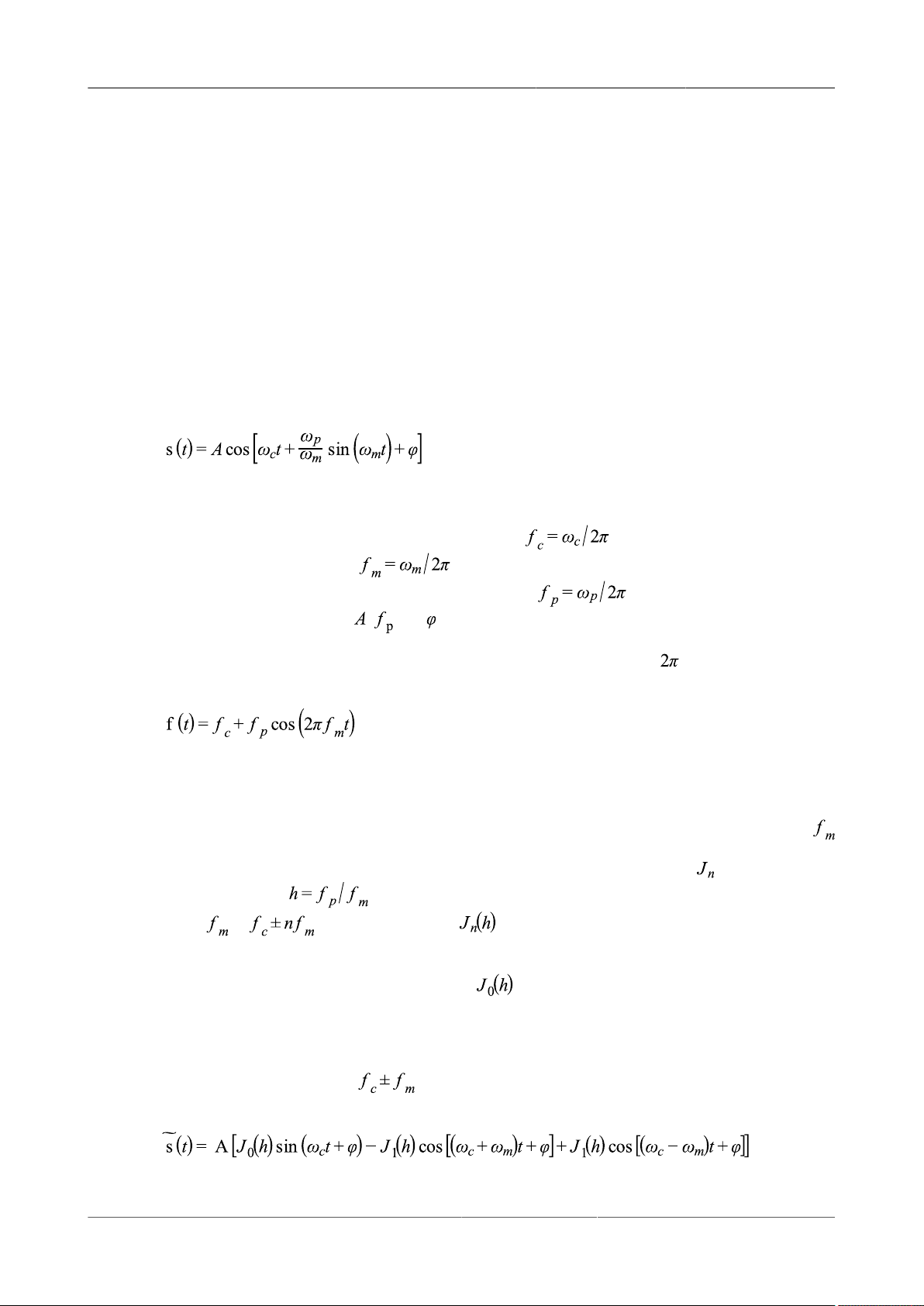
3.7. Tutorial Frequency Modulation

3.7.Tutorial Frequency Modulation

Note

This tutorial is addressed to HF2LI lock-in amplifier users that have purchased both HF2-MF multi-frequency and HF2-MOD AM/FM modulation options.

3.7.1.What is Frequency Modulation?

In frequency modulation (FM), the amplitude of the modulating signal is proportional to the instantaneous frequency deviation from a fixed frequency. In the simplest case shown in

Figure3.26(a), the modulated signal

Equation3.3.Frequency modulation

is produced when a carrier signal of frequency is modulated by a sinusoidal

modulation with frequency . The maximum variation of the frequency around the

carrier frequency, the peak frequency deviation, is . The physical information is

encoded in the parameters , and .

Because the frequency is the time derivative of the phase (divided by ) and the phase is the argument of the cosine in equation Equation3.3, we can define the instantaneous frequency as

Equation3.4.Instantaneous frequency

The spectrum of the FM signal of Equation3.3 is more complicated than in the case of amplitude modulation. It consists of the carrier and a series of pairs of sidebands at multiple integers of

around the carrier frequency, see Figure3.26(d). The amplitudes of the carrier and sidebands are given by mathematical functions called Bessel functions usually indicated by ) evaluated at the

modulation index . For instance, the n-th pair of sidebands is located symmetrically

about at and its amplitude is .

A peculiarity of the Bessel functions is that they oscillate around zero: even for the carrier, as the modulation index is increased, its amplitude decreases, crossing zero at h ≈ 2.41 and then

it increases in amplitude (in anti-phase) before reaching zero again at h ≈ 5.52.

At low modulation indexes, the amplitude of higher sidebands is very low and can thus be ignored: this is called the narrow-band approximation. In this limit (it is customary to assume h < 0.2),

only the two sidebands at have non-negligible amplitude and the signal s(t) can be approximated by

Equation3.5.Approximated narrow-band FM signal

HF2 User Manual - LabOne Edition Revision 34390 Zurich Instruments 72

Page 73

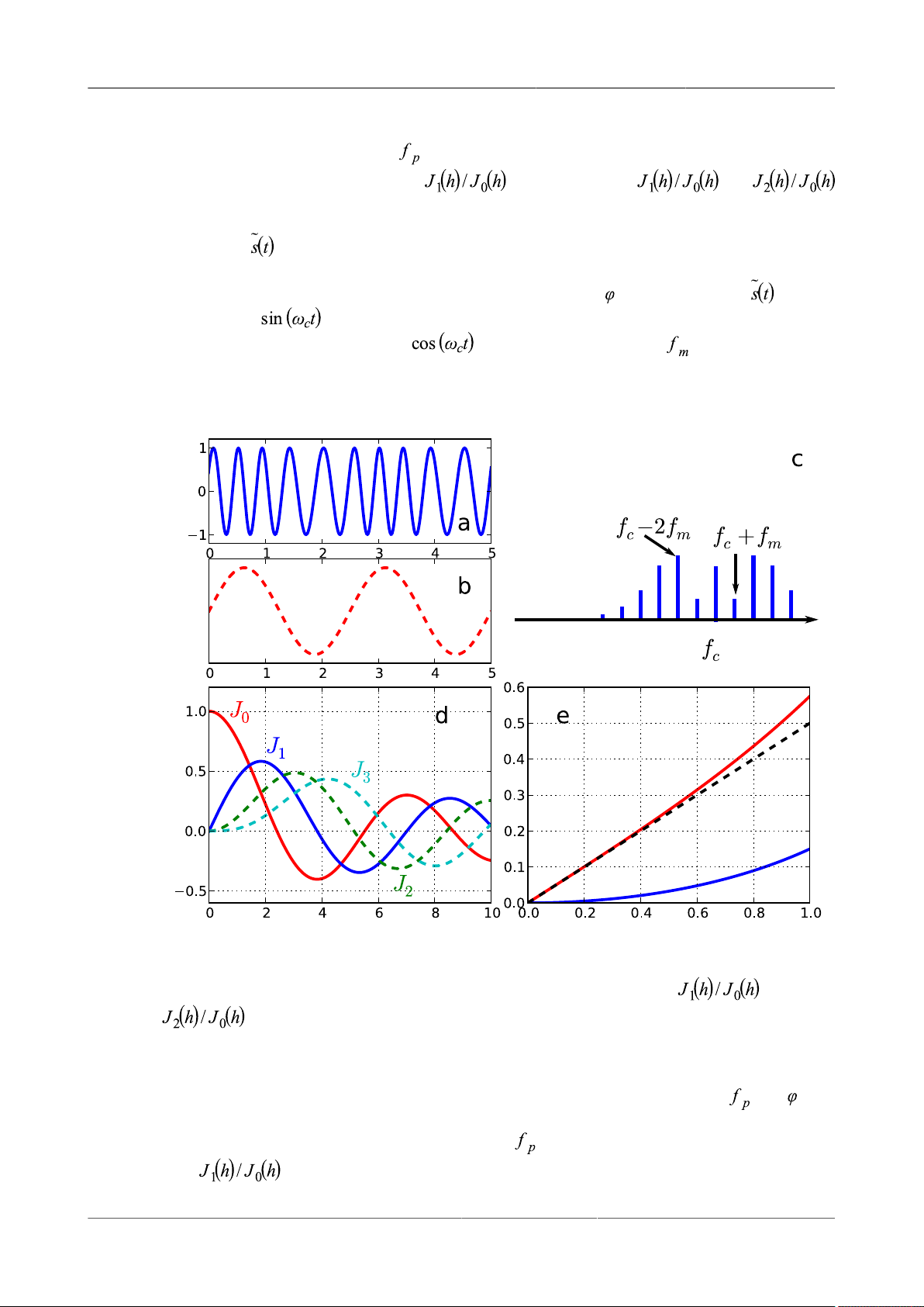
3.7. Tutorial Frequency Modulation

The first term is the carrier, the other two are the lower and upper sidebands. The problem of finding h (and the peak amplitude ) reduces now to comparing the amplitude of the first pair of

sidebands and the carrier to the ratio . A plot of the ratio and is shown in Figure3.26(e).

Even though looks very similar to an AM signal, there is a subtle but substantial difference: the phases of the sidebands are offset with respect to that of the carrier. This results in the sidebands

being in quadrature with the carrier. For example, assume that = 0: demodulating with the carrier signal gives the DC component (the carrier) but no sidebands; on the other hand, demodulating with the quadrature , only the two sidebands at are observed and no

carrier is present. Because of this, FM detection can be done in a similar way as AM detection scheme, using the tandem configuration described previously in Section3.6.1.

Figure3.26.(a) A simple frequency modulated signal, (b) its instantaneous frequency, (c) the frequency domain spectrum of a FM signal is composed of an infinite series of sidebands,

here depicted for h = 0.35, (d) n-th Bessel function versus h, (e) ratio (red line),

(blue line), slope 0.5 line (black dashed line)

The HF2-MOD AM/FM Modulation option permits direct generation and demodulation of an FM signal. For demodulation, this option enables measurement of the parameters A, , and .

Internally the HF2LI calculates the peak frequency with the method described above, from the

ratio , proportional to the carrier and first sideband amplitude. Since this method is

HF2 User Manual - LabOne Edition Revision 34390 Zurich Instruments 73

Page 74

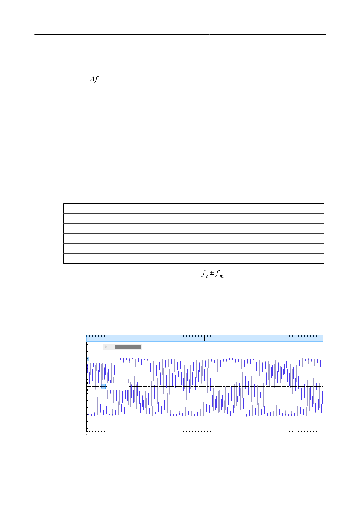
3.7. Tutorial Frequency Modulation

-0.15

-0.10

-0.05

-0.00

0.05

0.10

0.15

Y1: 1 fV

X1: 0.00000000 s

Y2: 1 fV Δ = 0.0000 V

X2: 0.00000000 s Δ = 0.00000000 s

valid only for narrow-band frequency modulation, users are advised to work at small values of the modulation index h < 1.

Another, intuitive way of demodulating an FM signal would be to use the PLL to track the frequency deviation and to further demodulate this signal. However, using sideband demodulation with the HF2-MOD AM/FM Modulation option provides a better signal-to-noise ratio. This is because

the signal can be averaged over several modulation cycles while keeping the bandwidth small.

3.7.2.Generate the Test Signal

In this tutorial, you are going to generate an FM signal with a carrier frequency of 1 MHz, a modulation frequency of 100 kHz, and a peak frequency of 50 kHz. The signal is generated at Signal Output 2 and is demodulated by the other lock-in unit by feeding it into Signal Input 1.

In the Modulation tab, in the Mod2 section, select the following parameters:

Table3.19.Settings: generate the FM signal

Carrier Oscillator (Osc)/Frequency Osc 1 / 1 MHz Sideband 1 Oscillator (Osc)/Frequency Osc 2 / 100 kHz MOD1 Mode/Enable FM / ON MOD2 Mode/Enable FM / ON MOD2 Carrier/Enable 100 mV / ON MOD2 Index/Enable 0.1 / ON

This generates an FM signal and two sidebands at . To look at this signal, connect Signal Output 2 to Signal Input 1 of the HF2 Instrument. Select the correct input parameters in the Lock-

in tab: for Signal Input 1, make sure Differential and 50 Ω are turned off. Then click the auto range button. In the Scope tab, select Signal Input 1 as Source, Signal Output 2 as Trigger, and click on Run/Stop to activate the Scope. Observe that the carrier amplitude is constant. The periodic frequency variation is hardly visible. In Frequency Domain FFT mode, the plot shows the carrier at 1 MHz and the two sidebands. You can increase the frequency resolution by selecting a smaller Sampling Rate and larger time scale in the Horizontal section of the Scope.

0 10 20 30 40 50 60 70

Wave (V)

Wave Channel 1

Time (μs)

HF2 User Manual - LabOne Edition Revision 34390 Zurich Instruments 74

Figure3.27.Time domain representation of the FM signal generated by MOD2 measured with the LabOne Scope

Page 75

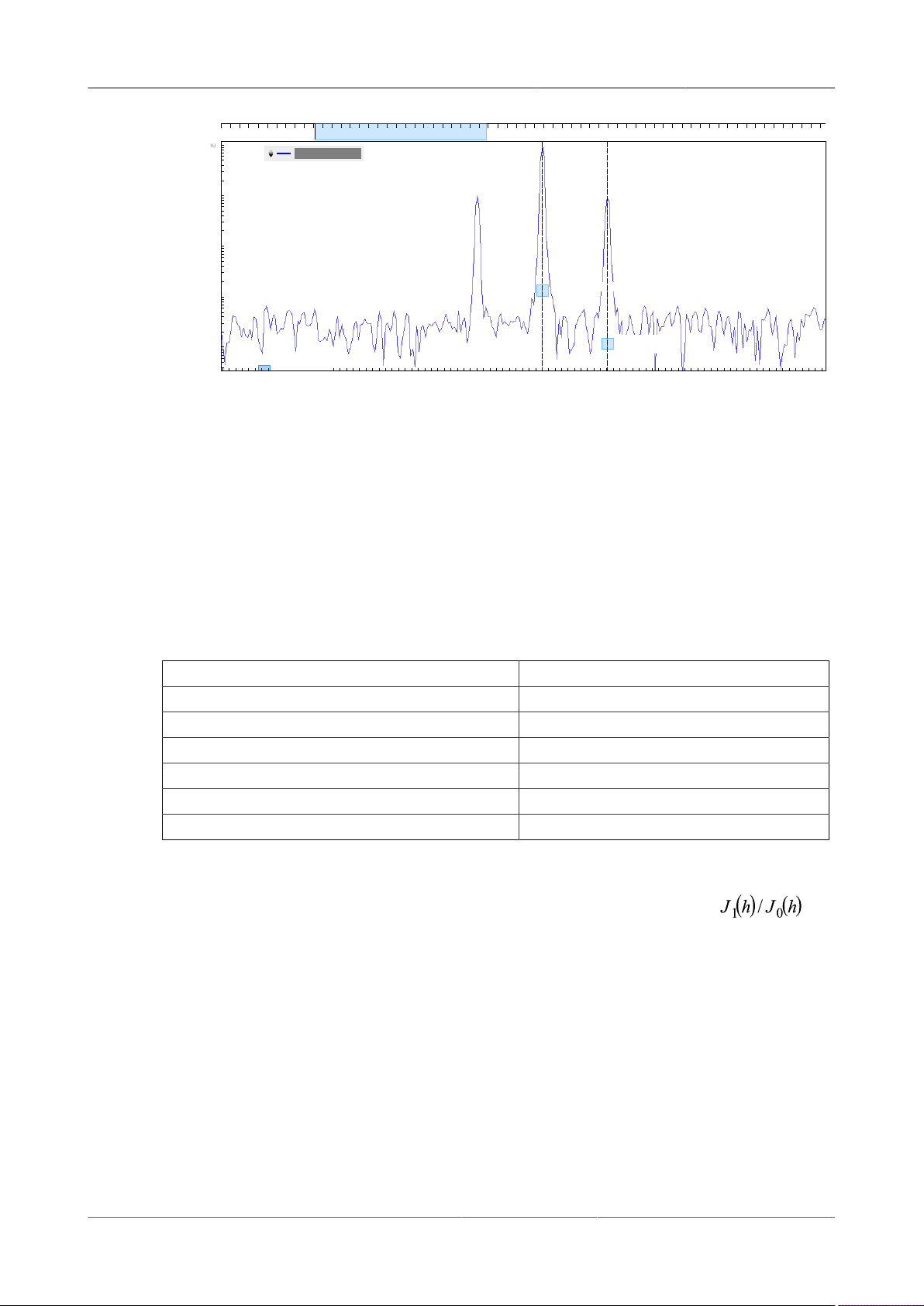
3.7. Tutorial Frequency Modulation

600 700 800 900 1000 1100 1200 1300 1400

-5

-4

-3

-2

-1

Y1: 1.0000 fV

X1: 1000.9 kHz

Y2: 1.0000 fV Δ = 0.0000 fV

X2: 1100.4 kHz Δ = 99.5 kHz

0 500 1000 1500 2000 2500 3000

Wave (V)

Wave Channel 1

Figure3.28.Frequency domain representation of the FM signal generated by MOD2 measured with the LabOne Scope

Frequency (kHz)

3.7.3.Measure the Test Signal

In the Modulation tab, in the Mod1 section, select the following parameters:

Table3.20.Measure the FM signal

Carrier oscillator (Osc) 1 Sideband 1 oscillator (Osc) 2 Mode FM Low-pass Filter BW (Carrier) 10 Hz Low-pass Filter BW (Sideband 1) 10 Hz MOD 1 Enable ON Demod 1, 2, 3 Data Transfer Enable (Lock-in tab) ON

This sets the correct demodulation of the FM signal. In the Numerical tab, look at the amplitude of the carrier, 71 mV

This corresponds approximately to the carrier amplitude multiplied by the ratio , see

Figure3.26(e) for our modulation index of h=0.2. Note that the phases of the two sidebands are

180° apart, which is typical for FM.

. You can also see that the two sidebands have an amplitude of 7.1 mV

RMS

HF2 User Manual - LabOne Edition Revision 34390 Zurich Instruments 75

Page 76

3.8. Tutorial Phase-locked Loop

3.8.Tutorial Phase-locked Loop

Note

This tutorial is applicable to HF2 Instruments with the HF2-PLL Dual Phase-locked Loop option installed.

3.8.1.Preparation

This tutorial explains how to track the resonance frequency shift of a quartz resonator using the PLL. To follow this tutorial, one simply needs to connect a resonator between Signal Output 1 and Signal Input 1.

3.8.2.Characterize the Resonator with the Sweeper

In this section you will learn first how to find the resonance of your resonator by measuring a frequency dependence in the Sweeper tab. The setup of the signal input, signal output, and data transfer in the Lock-in tab you know already from previous tutorials. In the Sweeper, one can start by defining a frequency sweep range from DC to 50 MHz and narrow down the range using multiple sweeps in order to find the resonance peak of interest. In our case, we know already that the resonance lies at around 1.8 MHz which saves us some time in finding the peak. The Sweeper tab and Lock-in tab setup is shown below.

Table3.21.Settings: acquire the reference signal

Tab Sub-tab Section # Label Setting / Value / State Lock-in 7 Output Amplitudes 1 Amp 1 (Vpk) / En 100.0 m / ON Lock-in 7 Signal Output 1  On ON Lock-in 1 Reference Osc 1 Lock-in 1 Signal Input Signal Sig In 1 Lock-in 1 Data Transfer PC En ON Sweeper Control Horizontal Sweep Param. Osc 1 Frequency Sweeper Control Horizontal Length 300 Sweeper Control Horizontal Start (Hz) 1.7 M Sweeper Control Horizontal Stop (Hz) 1.9 M Sweeper Control Horizontal  Dual Plot ON Sweeper Control Vertical Axis Groups 1 Demod R Add Signal Sweeper History History  Length 2 Sweeper Control  Run/Stop ON

In this tutorial, we are using the demodulator 7 to generate the sweep signal. We use demodulator 1 for measurement. The Lock-in settings ensure that the same oscillator (number 1) is used for

HF2 User Manual - LabOne Edition Revision 34390 Zurich Instruments 76

Page 77

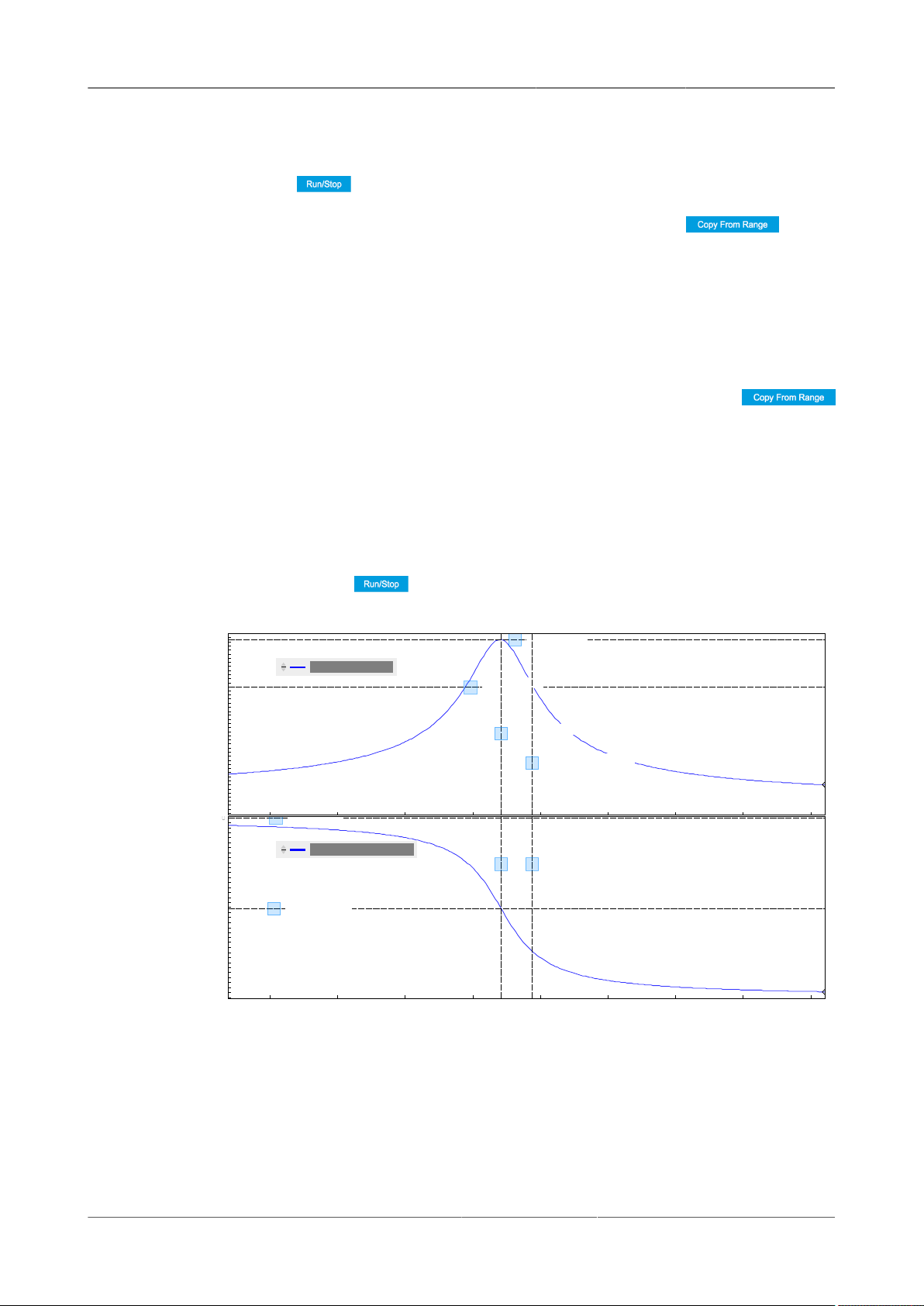
3.8. Tutorial Phase-locked Loop

-0.00

0.05

0.10

0.15 Y1: 0.1347 V

X1: 1842.94196 kHz

Y2: 0.1931 V Δ = 58.4 mV

X2: 1842.98839 kHz Δ = 0.04644 kHz

1.8426 1.8427 1.8428 1.8429 1.8430 1.8431 1.8432 1.8433 1.8434

-150

-100

-50

Y1: 0.0 deg

X1: 1842.94196 kHz

Y2: -91.0 deg Δ = -91.0 deg

X2: 1842.98839 kHz Δ = 0.04644 kHz

the sweep signal generation and for the demodulation. In addition, the input must be set to Signal Input 1.

Once the Sweeper button is clicked, the sweeper will repeatedly sweep the frequency response of the quartz oscillator. The user can then use the plot area tools explained in

Section4.1.3 to get a focus on the resonance peak of interest. Using the button,

the start and stop frequencies can easily be readjusted for a finer sweeper range. This will automatically enter the plot window range into the Start and Stop fields of the swept frequency range. The history length of 2 allows you to keep one previous sweep on the screen while adjusting the zoom.

Note

The sweep frequency resolution will get finer when zooming in horizontally using the button even without changing the number of points.

When a resonance peak has been found, you should get a spectrum similar to the plots shown in

Figure3.29. In this example, we have found the resonance peak at about 1.84 MHz. The X and Y

cursors help in extracting the precise resonance frequency as well as the half power bandwidth of about 93 Hz (note that this is the peak width at 1/sqrt(2) of the maximum signal amplitude). The phase response of the resonator reaches a value of about -90° at the resonance. We will use this value as a phase setpoint for the PLL. After having completed the Sweeper measurements, turn

off sweeping by clicking on . This will release the oscillator frequency from the control of the Sweeper.

Amplitude (V)

Phase (deg)

Demod 1 Sample R

Demod 1 Sample Phase

Figure3.29.Quartz resonator amplitude and phase response

Frequency (Hz)

×10

3.8.3.Resonance Tracking with the PLL

HF2 User Manual - LabOne Edition Revision 34390 Zurich Instruments 77

Page 78

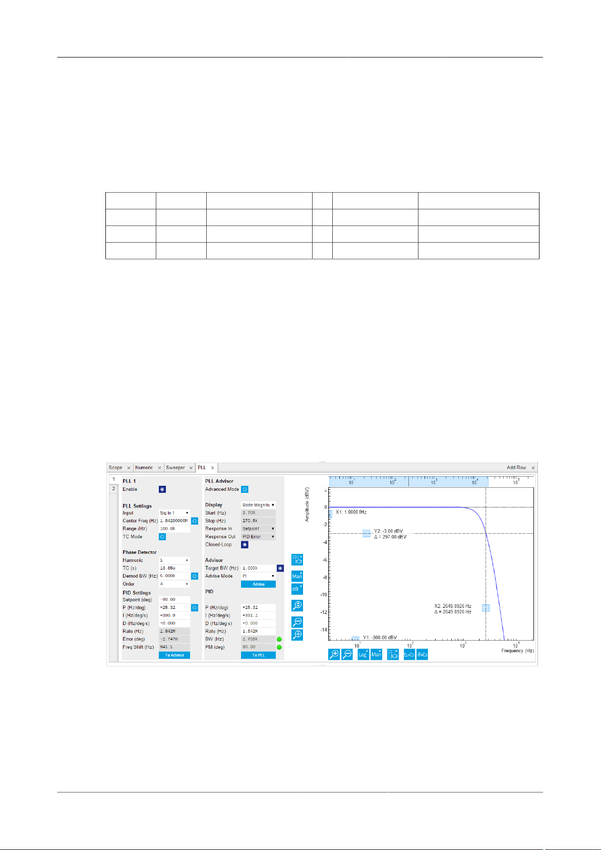
3.8. Tutorial Phase-locked Loop

Now that we have located the resonance frequency and its phase, we can now track the drift in resonance frequency by locking on the phase that we just measured using the Sweeper, hence the name phase-locked loop. The phase-locked loop is available under the PLL tab. There are two PLL controllers in each HF2 instrument. For this tutorial, we will use PLL 1. We first set up the basic PLL 1 fields as shown in the table below, using the resonator parameters determined using the Sweeper.

Table3.22.Settings: acquire the reference signal

Tab Sub-tab Section # Label Setting / Value / State PLL 1 PLL Settings Center Freq (Hz) 1.842 M / OFF PLL 1 PLL Settings  Range (Hz) 100 k PLL 1 PID Settings Setpoint (deg) -90

Next, we need to find suitable P, I, and D parameters. One can use the PLL Advisor for this purpose. For this tutorial, we will set the Target BW (Hz) to 1.0 k. The target bandwidth should be at least as large as the expected bandwidth of the frequency variations. In the present case, the resonator frequency is practically stable, so 1 kHz bandwidth is largely enough. Click on the Advise button to have the Advisor find a set of PID parameters using a numerical optimization algorithm. The Advisor tries to match or exceed the target bandwidth in its simulation. Figure3.30 shows the PLL tab after the Advisor has finished. In this case, the achieved bandwidth is about 2.7 kHz and can be read from the BW (Hz) field, or directly from the 3 dB point of the simulated Bode plot on the right. The Phase Margin value of the simulation is displayed in the PM (deg) field and should exceed 45° to ensure stable feedback operation without oscillations.

Once you are satisfied with the Advisor results, click on the To PLL button to copy the PID parameters to the physical PLL unit. To start the PLL operation, click on the Enable button on the top of the tab.

Figure3.30.PLL settings and simulation in the PLL tab

The frequency shift of the internal oscillator is shown in the field Freq Shift (Hz) and should now start to toggle. A successful phase lock is indicated by an Error (deg) toggling around zero, and a frequency shift that lies within the bounds -Range and +Range defined in the PLL settings.

HF2 User Manual - LabOne Edition Revision 34390 Zurich Instruments 78

Page 79

3.8. Tutorial Phase-locked Loop

Note

At this point, it is recommended to adjust the signal input range by clicking on the Auto Range button in the Lock-in tab. This will sometimes help the PLL to lock to an input signal with a

better noise performance.

The easiest way to visualize the frequency noise and drift is offered by the Plotter tool. One simply needs to select Frequency and Channel 1 and then click on Add Signal. The frequency noise increases with the PLL bandwidth, so for optimum noise performance the bandwidth should not be higher than what is required by the experiment. The frequency noise also scales inversely with the drive amplitude of the resonator.

HF2 User Manual - LabOne Edition Revision 34390 Zurich Instruments 79

Page 80

Chapter4.Functional Description LabOne User Interface

This chapter gives a detailed description of the functionality available in the LabOne User Interface (UI) for the Zurich Instruments HF2. LabOne provides a data server and a web server to control the Instrument with any of the most common web browsers (e.g. Firefox, Chrome, Edge, etc.). This platform-independent architecture supports interaction with the Instrument using various devices (PCs, tablets, smartphones, etc.) even at the same time if needed.

On top of standard functionality like acquiring and saving data points, this UI provides a wide variety of measurement tools for time and frequency domain analysis of measurement data as well as for convenient servo loop implementation.

HF2 User Manual - LabOne Edition Revision 34390 Zurich Instruments 80

Page 81

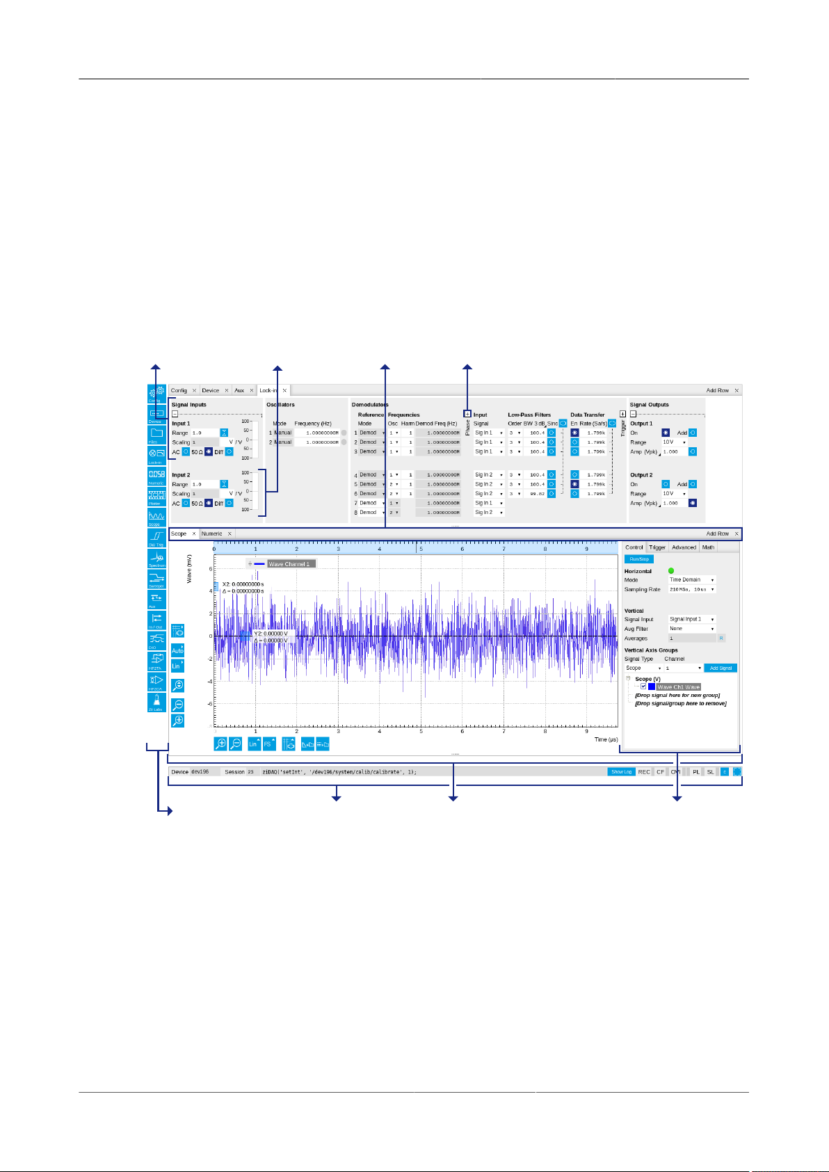
4.1. User Interface Overview

collapse/expand

side bar

unit 1

unit 2

status bar

tab bar

main area control tabs

4.1.User Interface Overview

4.1.1.UI Nomenclature

This section provides an overview of the LabOne User Interface, its main elements and naming conventions. The LabOne User Interface is a browser-based UI provided as the primary interface to the HF2. Multiple browser sessions can access the instrument simultaneously and the user can have displays on multiple computer screens. Parallel to the UI the Instrument can be controlled and read out (possibly concurrently) by custom programs written in any of the supported languages (e.g. LabVIEW, MATLAB, Python, C) connecting through the LabOne APIs.

Figure4.1.LabOne User Interface (default view)

Figure4.1 shows the default screen after a new measurements session has been started. The

UI is by default divided into two tab rows, each containing a tab structure that gives access to the different LabOne tools. Depending on display size and application, tab rows can be freely added and deleted with the control elements on the right-hand side of each tab bar. Similarly the individual tabs can be deleted or added by selecting app icons from the left side bar. A simple click on an icon adds the corresponding tab to the display, alternatively the icon can be dragged and dropped into one of the tab rows. Moreover, tabs can simply be displaced by drag-and-drop within a row or across rows. Further items are highlighted in Figure4.2.

HF2 User Manual - LabOne Edition Revision 34390 Zurich Instruments 81

Page 82

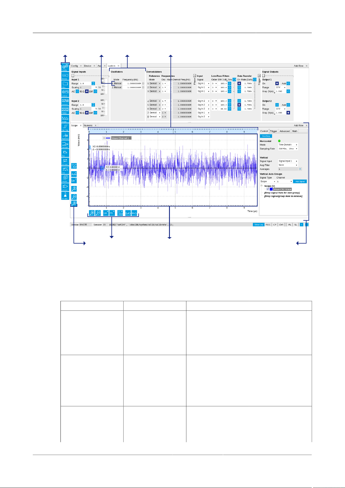
4.1. User Interface Overview

plot control icons

section

plot tab row

X rangeelement

app icons

Figure4.2.LabOne User Interface (more items)

Table4.1 gives s brief descriptions and naming conventions for the most important UI items.

Table4.1.LabOne User Interface features

Item name Position Description Contains side bar left-hand side of the UI contains app icons for

status bar bottom of the UI contains important

main area center of the UI accommodates all

app icons each of the available tabs - a click on an icon adds or activates the corresponding tab in the active tab row

status indicators status indicators, warning lamps, device and session information and access to the command log

tab rows, each active tabs - new rows can be added and removed by using the control elements in

consisting of tab bar

and the active tab area

HF2 User Manual - LabOne Edition Revision 34390 Zurich Instruments 82

Page 83

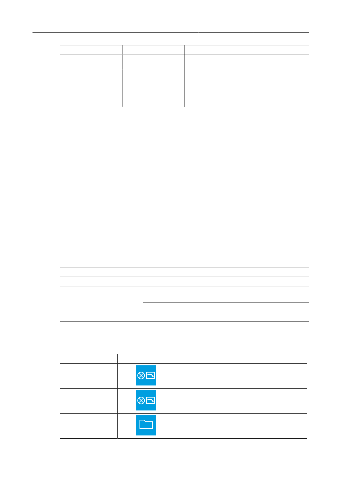
4.1. User Interface Overview

Item name Position Description Contains

tab area inside of each tab provides the active

4.1.2.Unique Set of Analysis Tools

All Instruments feature a comprehensive tool set for time and frequency domain analysis for both raw signals and demodulated signals. Note that the selection of app icons is limited by the upgrade options installed on a particular instrument.

The app icons on the left side of the UI can be roughly divided into two categories: settings and tools. Settings-related tabs are in direct connection of the instrument hardware allowing the user to control all the settings and instrument states. Tools-related tabs place a focus on the display and analysis of gathered measurement data. There is no strict distinction between settings and tools, e.g. will the Sweeper change certain demodulator settings while performing a frequency sweep. Within the tools one can further discriminate between time domain and frequency domain analysis, moreover, a distinction between the analysis of fast input signals - typical sampling rate of 210 MSa/s - and the measurement of orders of magnitude slower data - typical sampling rate of - derived for instance from demodulator outputs and auxiliary inputs. Table4.2 provides a brief classification of the tools.

the top right corner of each tab row

part of each tab consisting of settings, controls and measurement tools

sections, plots, control

tabs, unit selections

Table4.2.Tools for time domain and frequency domain analysis

Time Domain Frequency Domain Fast signals (210 MSa/s) Oscilloscope (Scope Tab) FFT analyzer (Scope Tab) Slow signals (<200 kSa/s)

The following table gives the overview of all app icons.

Table4.3.Overview of app icons and short description

Control/Tool Option/Range Description Lock-in Quick overview and access to all the settings

Lock-in MF Quick overview and access to all the settings

Files Access settings and measurement data files on

Numeric Spectrum Analyzer (Spectrum

Tab) Plotter Sweeper Software Trigger -

and properties for signal generation and demodulation.

the host computer.

HF2 User Manual - LabOne Edition Revision 34390 Zurich Instruments 83

Page 84

4.1. User Interface Overview

Control/Tool Option/Range Description Numeric Access to all continuously streamed

Plotter Displays various continuously streamed

Scope Displays shots of data samples in time and

SW Trig Provides complex trigger functionality on all

Spectrum Provides FFT functionality to all continuously

Sweeper Allows to scan one variable (of a wide choice,

Aux Controls all settings regarding the auxiliary inputs

measurement data as numerical values.

measurement data as traces over time (rollmode).

frequency domain (FFT) representation.

continuously streamed data samples and time domain display.

streamed measurement data.

e.g. frequency) over a defined range and display various response functions including statistical operations.

and auxiliary outputs.

In/Out Access to all controls relevant for the main Signal

Inputs and Signal Outputs on the instrument's front.

DIO Gives access to all controls relevant for the digital

inputs and outputs including the Ref/Trigger connectors.

Config Provides access to software configuration.

Device Provides instrument specific settings.

PID Features all control and analysis capabilities of

the PID controllers.

PLL Features all control and analysis capabilities of

the phase-locked loops.

MOD Control panel to enable (de)modulation at linear

combinations of oscillator frequencies.

HF2CA Remote control of the HF2CA Current Amplifier.

HF2 User Manual - LabOne Edition Revision 34390 Zurich Instruments 84

Page 85

4.1. User Interface Overview

Control/Tool Option/Range Description HF2TA Remote control of the HF2TA Current Amplifier.

ZI Labs Experimental settings and controls.

Table 4.4 gives a quick overview over the different status bar elements along with a short

description.

Table4.4.Status bar description

Control/Tool Option/Range Description Command log last command Shows the last command. A different formatting

Show Log Show the command log history in a separate

Session integer value Indicates the current session identifier. Device devXXX Indicates the device serial number. REC grey/green A green indicator shows ongoing data recording

CF grey/yellow/red Clock Failure - Red: present malfunction of the

OVI grey/yellow/red Signal Input Overflow - Red: present overflow

OVO grey/yellow/red Overflow Signal Output - Red: present overflow

PL grey/yellow/red Packet Loss - Red: present loss of data between

SL grey/yellow/red Sample Loss - Red: present loss of sample data

C Reset status flags: Clear the current state of the

MOD grey/green MOD - Green: indicates which of the modulation

PID grey/green PID - Green: indicates which of the PID units is

(Matlab, Python, ..) can be set in the config tab. The log is also saved in [User]\Documents\Zurich Instruments\LabOne\WebServer\Log

browser window.

(related to global recording settings in the Config tab).

external 10 MHz reference oscillator. Yellow: indicates a malfunction occurred in the past.

condition on the signal input also shown by the red front panel LED. Yellow: indicates an overflow occurred in the past.

condition on the signal output. Yellow: indicates an overflow occurred in the past.

the device and the host PC. Yellow: indicates a loss occurred in the past.

between the device and the host PC. Yellow: indicates a loss occurred in the past. Note: a possible reason for high sample loss may be caused by a scope running in parallel.

status flags

kits is enabled.

enabled.

HF2 User Manual - LabOne Edition Revision 34390 Zurich Instruments 85

Page 86

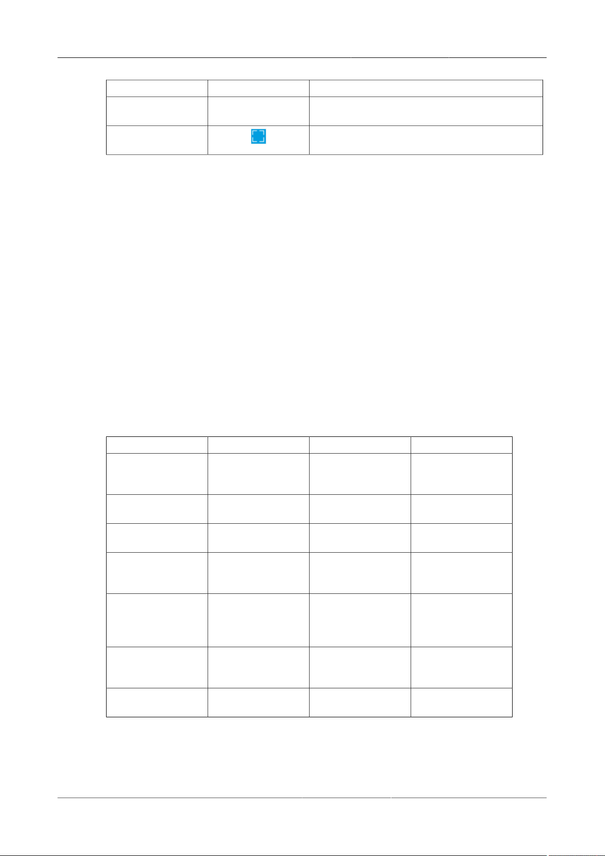
4.1. User Interface Overview

Control/Tool Option/Range Description PLL grey/green PLL - Green: indicates which of the PLLs is

Full Screen Toggles the browser between full screen and

4.1.3.Plot Functionality

Several tools - Plotter, Scope, SW Trigger, Spectrum - provide a graphical display of measurement data in the form of plots. These are multi-functional tools with zooming, panning and cursor capability. This section introduces some of the highlights.

Plot area elements

Plots consist of the plot area, the X range and the range controls. The X range (above the plot area) indicates which section of the wave is displayed by means of the blue zoom region indicators. The two ranges show the full scale of the plot which does not change when the plot area displays a zoomed view. The two axes of the plot area instead do change when zoom is applied.

enabled.

normal mode.

The mouse functionality inside of plot is summarized in Table4.5

Table4.5.Mouse functionality inside plots

Name Action Description Performed inside Panning left click on any

location and move around

Zoom X axis mouse wheel zooms in and out the

Zoom Y axis shift + mouse wheel zooms in and out the

Window zoom shift and left mouse

area select

Absolute jump of zoom area

Absolute move of zoom area

Full Scale double click set X and Y axis to full

left mouse click moves the blue zoom

left mouse drag-anddrop

moves the waveforms

X axis

Y axis selects the area of

the waveform to be zoomed in

range indicators

moves the blue zoom range indicators

scale

plot area

X and Y range, but outside of the blue zoom range indicators

X and Y range, inside of the blue range indicators

plot area

Each plot area contains a legend that lists all the shown signals in the respective color. The legend can be moved to any desired position by means of drag-and-drop.

The X range and Y range plot controls are described in Table4.6.

HF2 User Manual - LabOne Edition Revision 34390 Zurich Instruments 86

Page 87

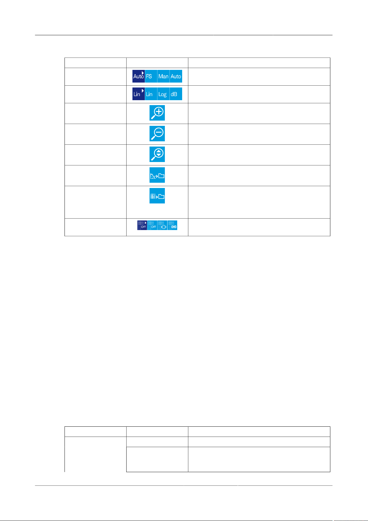
4.1. User Interface Overview

Table4.6.Plot control description

Control/Tool Option/Range Description Axis scaling mode Selects between automatic, full scale and manual

Axis mapping mode Select between linear, logarithmic and decibel

Axis zoom in Zooms the respective axis in by a factor of 2.

Axis zoom out Zooms the respective axis out by a factor of 2.

Rescale axis to data Rescale the foreground Y axis in the selected

Save figure Generates an SVG of the plot area or areas for

Save data Generates a TXT consisting of the displayed set

Cursor control Cursors can be switch On/Off and set to be moved

axis scaling.

axis mapping.

zoom area.

dual plots to the local download folder.

of samples. Select full scale to save the complete wave. The save data function only saves one shot at a time (the last displayed wave).

both independently or one bound to the other one.

Cursors and Math

The plot area provides two X and two Y cursors which appear as dashed lines inside of the plot area. The four cursors are selected and moved by means of the blue handles individually by means of drag-and-drop. For each axis there is a primary cursor indicating its absolute position and a secondary cursor indicating both absolute and relative position to the primary cursor.

Cursors have an absolute position which does not change by pan or zoom events. In case the cursors move out of the zoom area, the corresponding handle is displays on the related side of the plot area. Unless the handle is moved, the cursor keeps the current position. This functionality is very effective to measure large deltas with high precision (as the absolute position of the other cursors does not move).

The cursor data can also be used to define the input data for the mathematical operations performed on plotted data. This functionality is available in the Math sub-tab of each tool. The following Table4.7 gives an overview of all the elements and their functionality. It is important to know that the Signals and Operations defined will always be performed only on the currently chosen active trace.

Table4.7.Plot math description

Control/Tool Option/Range Description

Cursor Loc Cursor coordinates as input data.Source Select

Cursor Area Consider all plot data inside the rectangle defined

by the cursor coordinates as input for statistical functions (Min, Max, Avg, Std, Int).

HF2 User Manual - LabOne Edition Revision 34390 Zurich Instruments 87

Page 88

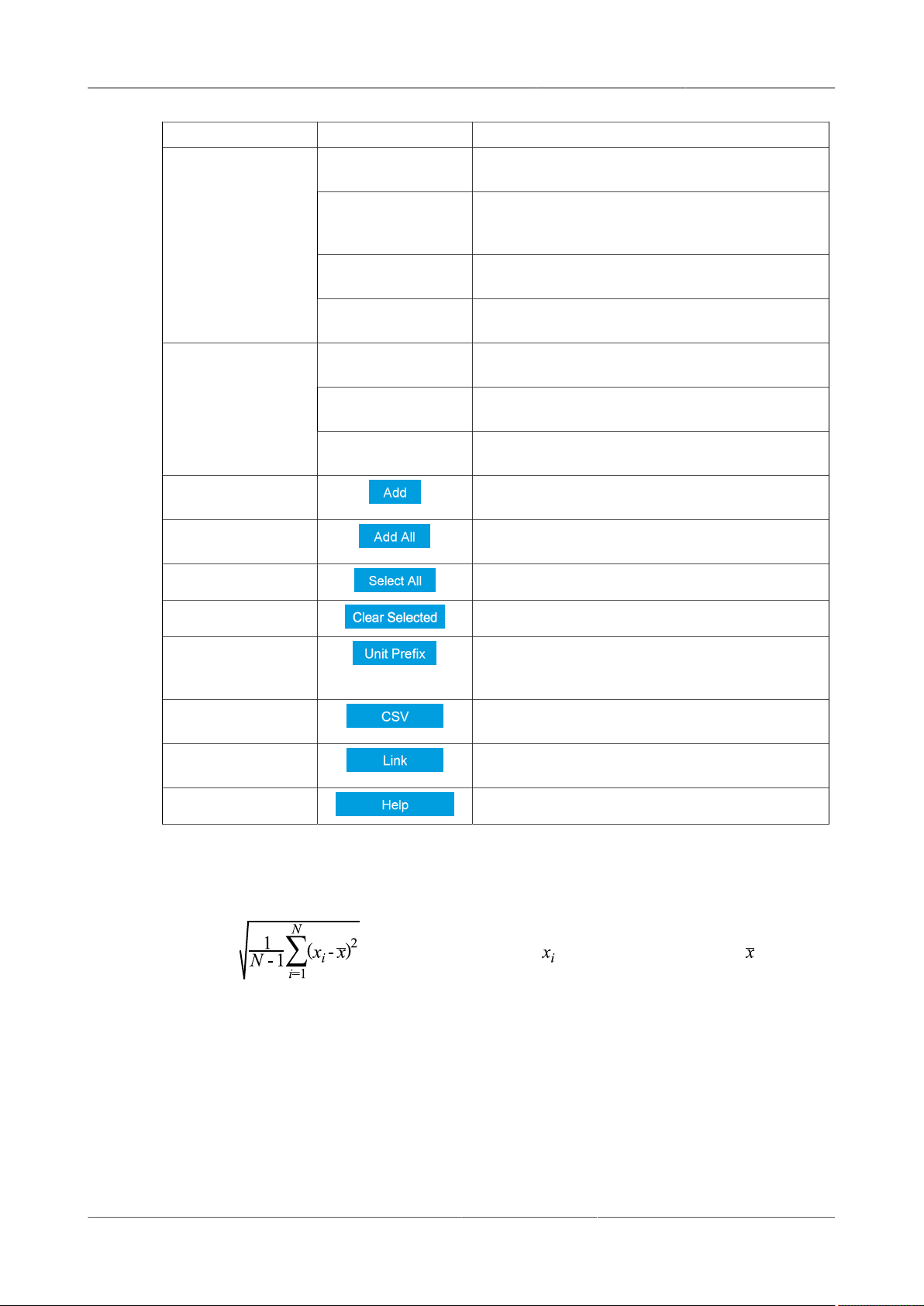
4.1. User Interface Overview

Control/Tool Option/Range Description

Operation Select

Add Add the selected math function to the result table

Add All Add all operations for the selected signal to the

Select All Select all lines from the result table above.

Tracking Output plot value at current cursor position.

Options are X1 and X2.

Wave Consider all plot data currently displayed in the

Plot as input for statistical functions (Min, Max, Avg, Std, Int).

Peak Find and determine the various peaks in the

plotted data and their associated values.

Histogram Select statistical data as Math input and display

a histogram in the plot area.

X1, X2, X2-X1,

Y1, Y2, Y2-Y1

Min, Max,

Avg, Std, Int

Pos, Level Finds the Position (x-values) and the Levels (y-

Cursors values and their differences.

Statistical Functions applied to a set of samples.

values) of Peaks on a set of samples.

below.

result table below.

Clear Selected Clear selected lines from the result table above.

Unit Prefix Adds a suitable prefix to the SI units to allow for

better readability and increase of significant digits displayed.

CSV Values of the current result table are saved as a

text file into the download folder.

Link Provides a LabOne Net Link to use the data in

tools like Excel, Matlab, etc.

Help Opens the LabOne User Interface help.

Note

For calculation of the standard deviation the corrected sample standard deviation is used as

defined by with a total of N samples and an arithmetic average .

Tree Sub-Tab

The Numeric tab and Plotter tab are able to display so many different types of signals that a number of different options are provided to access them. One of them is the Tree sub-tab that allows essentially to access all streamed measurement data in a hierarchical structure by checking the boxes of the signal that should be displayed.

HF2 User Manual - LabOne Edition Revision 34390 Zurich Instruments 88

Page 89

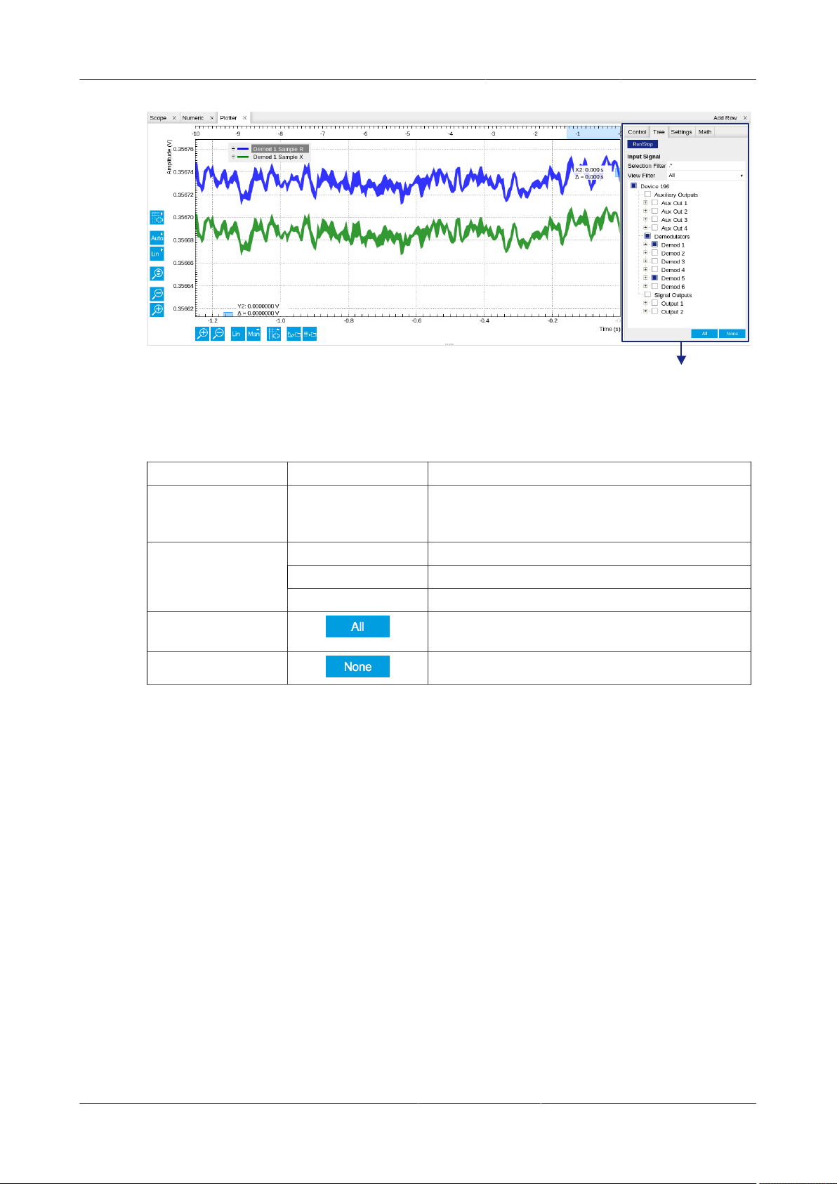
4.1. User Interface Overview

Tree sub-tab

Figure4.3.Tree sub-tab in Plotter tab

Table4.8.Tree description

Control/Tool Option/Range Description Selection Filter Regular expression Create a filter to define which streaming nodes

View Filter

All Select all nodes that can be selected in the

None Unselect all nodes.

are selected. The View Filter presents a number of presets that can serve as examples.

All Show all available nodes.

R,X,Y Show demodulator streaming nodes.

Streams Show all streaming nodes.

relevant context.

Vertical Axis Groups

Vertical Axis groups are available in the Plotter tab, SW Trigger tab, and Sweeper tab. These tools are able to show signals with different axis properties within the same plot. As a frequency and amplitude axis have fundamentally different limits they have each their individual axis which allows for correct auto scaling. However, signals of the same type e.g. Cartesian demodulator results should preferably share one scaling. This allows for fast signal strength comparison. To achieve this the signals are assigned to specific axis group. Each axis group has its own axis system. This default behavior can be changed by moving one or more signals into a new group.

HF2 User Manual - LabOne Edition Revision 34390 Zurich Instruments 89

Page 90

4.1. User Interface Overview

Vertical Axis Groups

Figure4.4.Vertical Axis Group in Plotter tool

The tick labels of only one axis group can be shown at once. This is the foreground axis group. To define the foreground group click on one of the group names in the Vertical Axis Groups box. The current foreground group gets a high contrast color.

Select foreground group: Click on a signal name or group name inside the Vertical Axis Groups. If a group is empty the selection is not performed.

Split the default vertical axis group: Use drag-and-drop to move one signal on the field [Drop signal here to add a new group]. This signal will now have its own axis system.

Change vertical axis group of a signal: Use drag-and-drop to move a signal from one group into

another group that has the same unit.

Group separation: In case a group hosts multiple signals and the unit of some of these signals changes, the group will be split in several groups according to the different new units.

Remove a signal from the group: In order to remove a signal from a group drag-and-drop the signal to a place outside of the Vertical Axis Groups box.

Remove a vertical axis group: A group is removed as soon as the last signal of a custom group is removed. Default groups will remain active until they are explicitly removed by drag-and-drop. If a new signal is added that match the group properties it will be added again to this default group. This ensures that settings of default groups are not lost, unless explicitly removed.

Rename a vertical axis group: New groups get a default name 'Group of ...'. This name can be changed by double-clicking on the group name.

Hide/show a signal: Uncheck/check the check box of the signal. This is faster than fetching a signal from a tree again.

Figure4.5.Vertical Axis Group typical drag and drop moves

HF2 User Manual - LabOne Edition Revision 34390 Zurich Instruments 90

Page 91

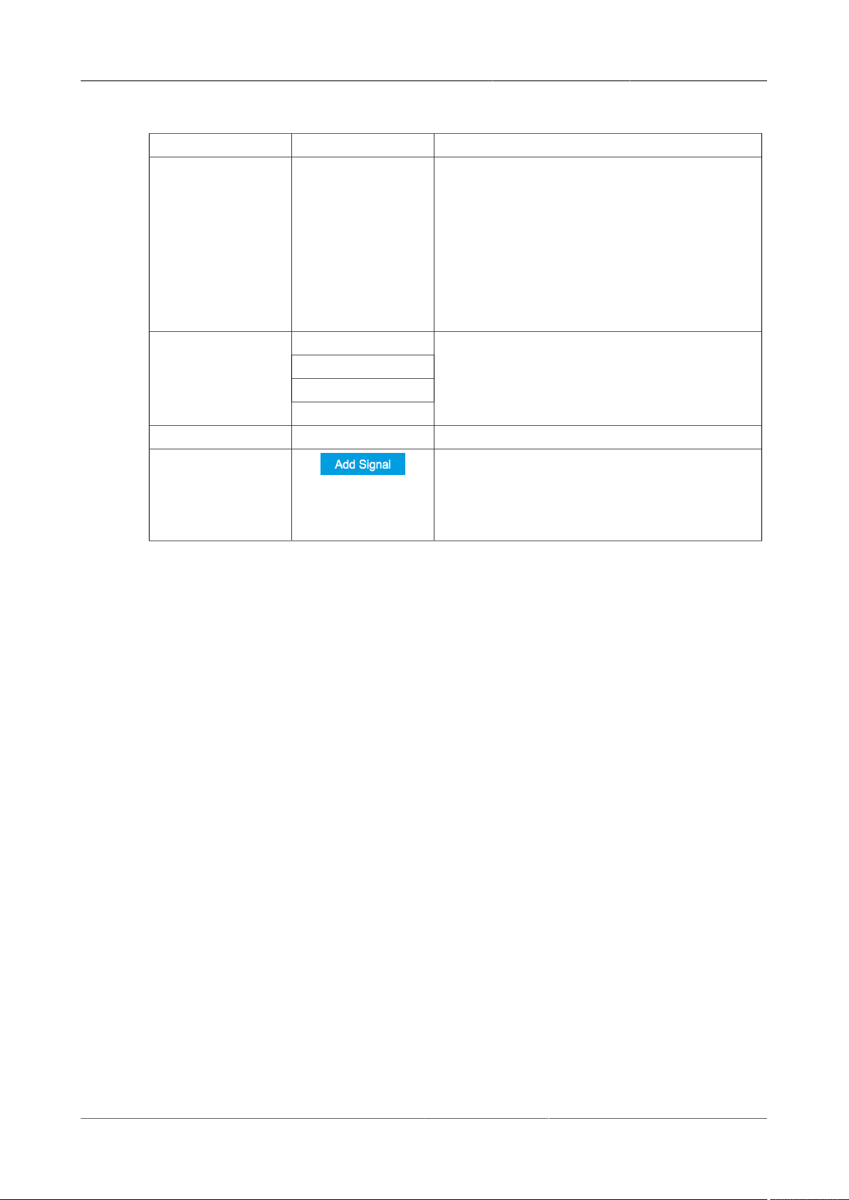
4.1. User Interface Overview

Table4.9.Vertical Axis Groups description

Control/Tool Option/Range Description Vertical Axis Group  Manages signal groups sharing a common

Signal Type

Channel integer value Selects a channel to be added. Add Signal Adds a signal to the plot. The signal will be added

Demod X, Y, R, Theta

Frequency

Aux Input 1, 2

HW Trigger

vertical axis. Show or hide signals by changing the check box state. Split a group by dropping signals to the field [Drop signal here to add new group]. Remove signals by dragging them on a free area.

Rename group names by editing the group label. Axis tick labels of the selected group are shown in the plot. Cursor elements of the active wave (selected) are added in the cursor math tab.

Select signal types for the Vertical Axis Group.

to its default group. It may be moved by drag and drop to its own group. All signals within a group share a common y-axis. Select a group to bring its axis to the foreground and display its labels.

HF2 User Manual - LabOne Edition Revision 34390 Zurich Instruments 91

Page 92

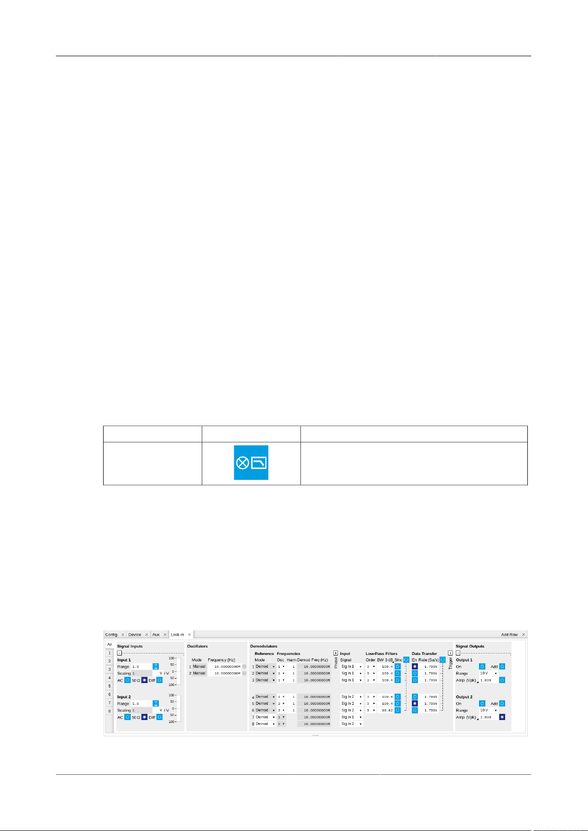
4.2. Lock-in Tab

4.2.Lock-in Tab

This tab is the main lock-in amplifier control panel. Users with instruments with HF2-MF Multifrequency option installed are kindly referred to Section4.3.

4.2.1.Features

• Functional block diagram with access to main input, output and demodulator controls

• Parameter table with main input, output and demodulator controls

• Control elements for 6 configurable demodulators

• Auto ranging, scaling, arbitrary input units for both input channels

• Control for 2 oscillators

• Settings for main signal inputs and signal outputs

• Flexible choice of reference source, trigger options and data transfer rates

4.2.2.Description

The Lock-in tab is the main control center of the instrument and open after start up by default. Whenever the tab is closed or an additional one of the same type is needed, clicking the following icon will open a new instance of the tab.

Table4.10.App icon and short description

Control/Tool Option/Range Description Lock-in Quick overview and access to all the settings

The default view of the Lock-in tab is the parameter table view. It is accessible under the sidetab labeled All and provides controls for all demodulators in the instrument. Moreover, for each individual demodulator there is a functional block diagram available. It is accessible under the side-tab labeled with the corresponding demodulator number.

Parameter Table

The parameter table (see Figure 4.6) consists of 4 vertical sections: Signal Inputs, Oscillators, Demodulators and Signal Outputs. The Demodulators sections gives access to all the settings of demodulators 1 to 6 that can be used for measurement, and of demodulators 7 and 8 that can be used for external referencing. Demodulators 1 to 3 (4 to 6) are connected to Signal Input 1 (2).

and properties for signal generation and demodulation.

Figure4.6.LabOne User Interface Lock-in tab - Parameter table (All)

HF2 User Manual - LabOne Edition Revision 34390 Zurich Instruments 92

Page 93

4.2. Lock-in Tab

Harm onic

Phase Shift

Low-pass Filter

Mixer

Down Sample

Aux Out

PID

Aux Out

PID

Polar

Demodulators 1-6

Oscillator

Signal Input

Oscillator

Signal Input

BW, Order

Rate

n Phase

+ 90°

Harm onic Phase Shift

Low-pass Filter

Mixer

Down Sample

PLL

Polar

Demodulators 7-8

BW, Order

n= 1,2

+ 90°

Signal Output

The Signal Inputs section allows the user to define all relevant settings specific to the signal entered as for example input coupling, range, etc. Some of the available options like phase adjustment and the trigger functionality are collapsed by default. It takes one mouse click on the "+" icon in order to expand those controls. On the right-hand side of the Lock-in tab the Signal Outputs section allows defining signal amplitudes, offsets and range values.

Below the Scaling field there is the AC/DC button and the 50 Ω/1 MΩ. The AC/DC button sets the coupling type: AC coupling has a high-pass cutoff frequency that can be used to block large DC signal components to prevent input signal saturation during amplification. The 50 Ω/1 MΩ button toggles the input impedance between low (50 Ω) and high (approx. ) input impedance. With 50 Ω input impedance, one will expect a reduction of a factor of 2 in the measured signal if the signal source also has an output impedance of 50 Ω. Next to the 50 Ω button, there is the Diff button which switches the Signal Input between a single-ended measurement on the + Input and a differential measurement on the + and - Inputs.

The Oscillator section indicates the frequencies of both internal oscillators. Where the Mode indicator shows Manual, the user can define the oscillator frequency manually defined by typing a frequency value in the field. In case the oscillator is referenced to an external source, the Mode indicator will show ExtRef and the frequency field is set to read-only. External reference requires a PLL to do the frequency mapping onto an internal oscillator. Successful locking is indicated by a green light right next to the frequency field. When the Modulation unit or the PID controller determine the frequency value of an oscillator, MOD or PID are indicated in the Mode field and the user cannot change the frequency manually.

In the following, we discuss the Demodulators settings in more detail. The block diagram displayed in Figure4.7 indicates the main demodulator components and their interconnection. The understanding of the wiring is essential for successfully operating the instrument.

Figure4.7.Demodulator block diagram without HF2-MF Multi-frequency option.

HF2 User Manual - LabOne Edition Revision 34390 Zurich Instruments 93

Page 94

4.2. Lock-in Tab

The first 6 lines in the Demodulators section represent the demodulators available for measurements. The Mode column is read-only set to internal reference (Demod). The 7th and 8th line represent a additional demodulators that are reserved for the exclusive use as phase detectors when the mode is switched to external reference (ExtRef). In ExtRef mode, the user can select from a number of different inputs to be used as external reference signal. However, the demodulators 7 and 8 do not produce any output data that could be used for measurements.

In the Input Signal column one selects the signal that is taken as input for a given demodulator among the two Signal Inputs.

For each demodulator an additional phase shift can be introduced to the associated oscillator by entering the phase offset in the Phase column. This phase is added both to the reference channel and to the output of the demodulator. Hence, when the frequency is generated and detected using the same demodulator, signal phase and reference phase change by the same amount and no change will be visible in the demodulation result. Demodulation of frequencies that are integer multiples of any of the oscillator frequencies is achieved by entering the desired factor in the Harm column. The result of the demodulation, i.e. the amplitude and phase can be read e.g. using the Numeric tab which is described in Section4.4.

In the middle of the Lock-in tab is the Low-Pass Filters section where the filter order can be selected in the drop-down list for each demodulator and the filter bandwidth (BW 3dB) can be chosen by typing a numerical value. Alternatively, the time constant of the filter (TC) or the noise equivalent power filter bandwidth (BW NEP) can be chosen by clicking on the column's header. For example, setting the filter order to 4 corresponds to a roll off of 24 dB/oct or 80 dB/dec i.e. an attenuation of 104 for a tenfold frequency increase. If the Low-Pass Filter bandwidth is comparable to or larger than the demodulation frequency, the demodulator output may contain frequency components at the frequency of demodulation and its higher harmonics. In this case, the additional Sinc Filter should be enabled. It attenuates those unwanted harmonic components in the demodulator output. The Sinc Filter is useful when measuring at low frequencies, since it allows one to apply a Low-Pass Filter bandwidth closer to the demodulation frequency, thus speeding up the measurement time.

The data transfer of demodulator outputs is activated by the En button in the Data Transfer section where also the sampling rate (Rate) for each demodulator can be defined.

The Trigger section next to the Data Transfer allows for setting trigger conditions in order to control and initiate data transfer from the Instrument to the host PC by the application of logic signals (e.g. TTL) to either DIO 0 or 1 on the instrument back panel.

In the Signal Outputs section the On buttons are used to activate the Signal Outputs. This is also the place where the output amplitudes for the Signal Outputs can be set in adjustable units (Vpk, Vrms, or dBm). The Range drop-down list is used to select the proper output range setting. By enabling the Add button, one can add an external analog signal which is applied to the Add input to the Signal Output.

Block Diagram

The block diagram view of the main instrument functions is also sometimes called the "Graphical Lock-in Tab". A set of indexed side-tabs in the Lock-in Tab give access to a block diagram for each demodulator. The block diagrams are fully functional and provide the user with a visual feedback of what is going on inside the instrument. All control elements that are available in the Parameter Table detailed in the previous section are also present in the graphical representation.

The block diagram in Figure4.8 shows the signal path through the instrument for the case when the internal oscillator is used as reference. The Signal Inputs and Reference/Internal Frequency are shown on the left-hand side. The actual demodulation, i.e. the mixing and low-pass filtering

HF2 User Manual - LabOne Edition Revision 34390 Zurich Instruments 94

Page 95

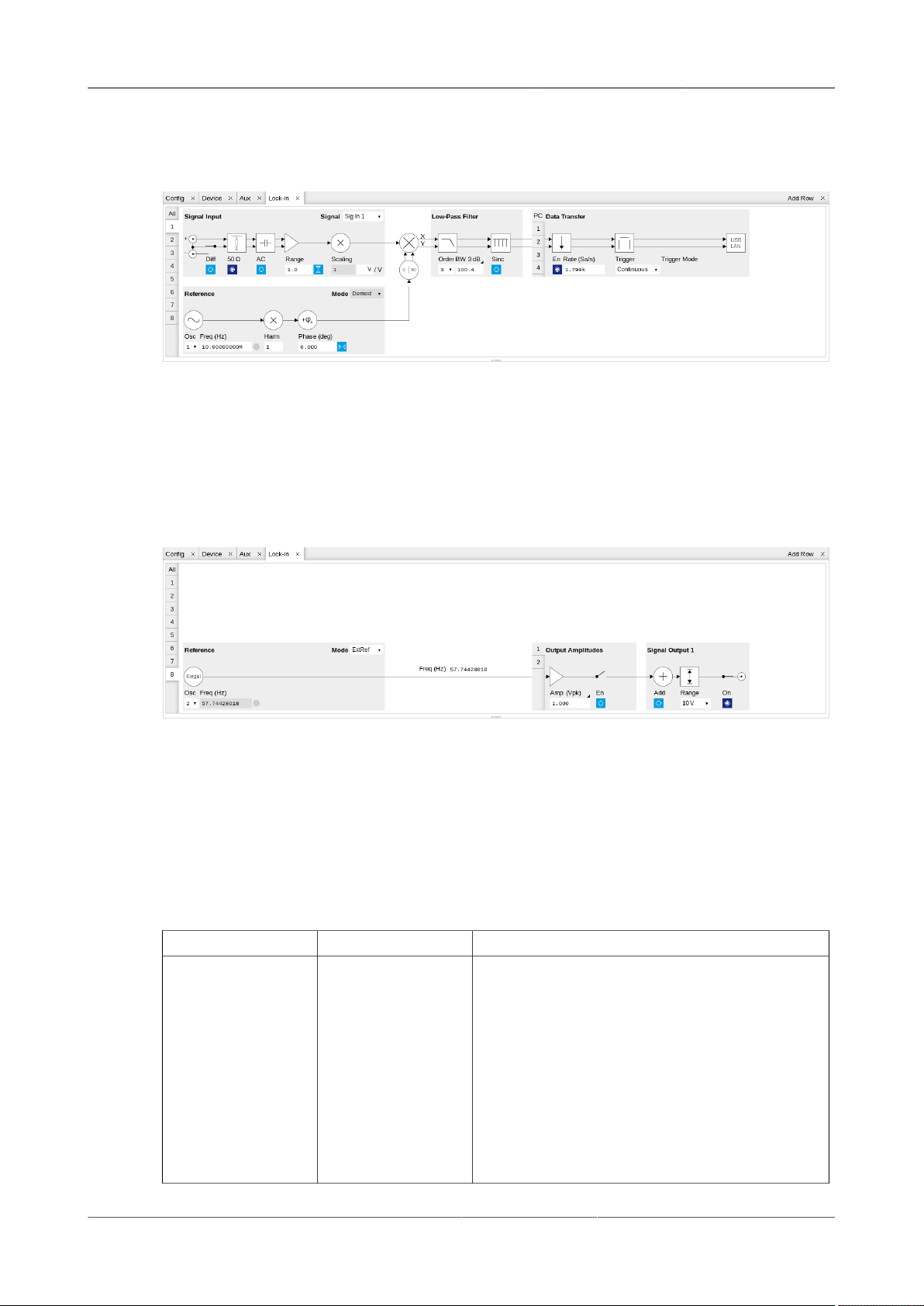
4.2. Lock-in Tab

is represented in the center of the tab. On the bottom right the user can set Signal Output parameters. On the top right there are the settings related to the output of the measurement data, either by digital means (PC Data Transfer) or by analog means (Auxiliary Outputs 1 to 4).

Figure4.8.LabOne User Interface Lock-in tab - Graphical Lock-in tab in Internal Reference mode

The block diagram in Figure4.9 shows the signal path through the instrument for the case when an external reference is used. This setting is only available for demodulators 7 and 8. In order to map an external frequency to oscillator 1/2 go to the Reference section of demodulator 7/8 and change the mode to ExtRef. This demodulator will then be used as a phase detector within a phase locked loop. The software will choose the appropriate filter settings according to the frequency and properties of the reference signal.

Figure4.9. LabOne User Interface Lock-in tab - Graphical Lock-in tab in External Reference mode

4.2.3.Functional Elements

Table4.11.Lock-in tab

Control/Tool Option/Range Description Range 1 mV to 1.5 V Defines the gain of the analog input amplifier.

The range should exceed the incoming signal by roughly a factor two including a potential DC offset.

Note 1: the value inserted by the user may be approximated to the nearest value supported by the Instrument. Note 2: a proper choice of range setting is crucial in order to achieve good accuracy and best possible signal to noise ratio as it targets to use the full dynamic range of the input ADC.

HF2 User Manual - LabOne Edition Revision 34390 Zurich Instruments 95

Page 96

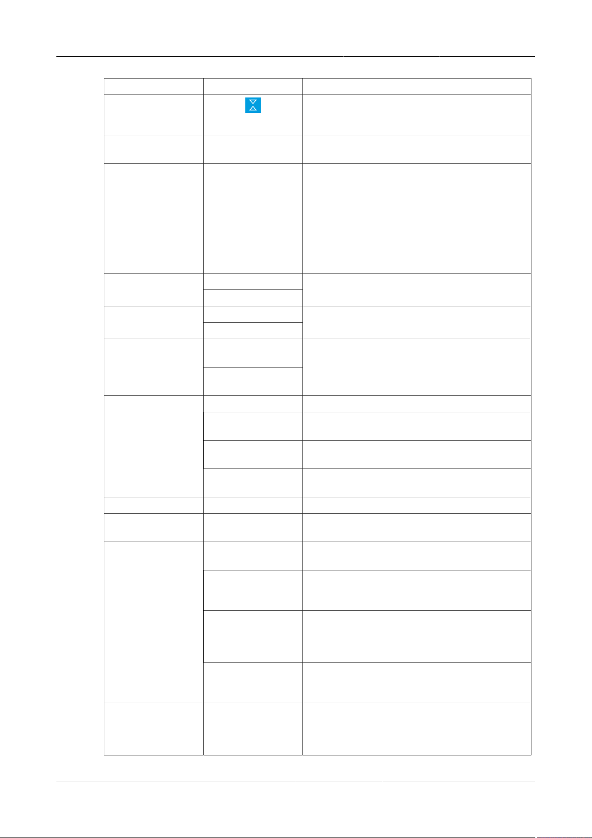
4.2. Lock-in Tab

Control/Tool Option/Range Description Auto Automatic adjustment of the Range to about

Scaling numeric value Applies an arbitrary scale factor to the input

Measurement Unit unit acronym Defines the physical unit of the input signal. Use

Diff

Mode

Frequency (Hz) 0 to 50 MHz Frequency control for each oscillator. Locked ON / OFF Oscillator locked to external reference when

Mode

Osc oscillator index Connects the selected oscillator with the

two times the maximum signal input amplitude measured over about 100 ms.

signal.

*, / and ^ operators, e.g., 'm' or 'm/s^2'.

The value in this field modifies the readout of all measurement tools in the user interface. Typical uses of this field is to make measurements in the unit before the sensor/transducer, e.g. to take an transimpedance amplifier into account and to directly read results in Ampere instead of Volts.

ON: AC couplingAC

OFF: DC coupling

ON: 50 Ω50 Ω

OFF: 1 MΩ

OFF: Single ended

voltage input

ON: Differential

voltage input

Manual The user setting defines the oscillator frequency.

ExtRef An external reference is mapped onto the

PLL The HF2-PLL option controls the oscillator

PID The HF2-PID option controls the oscillator

Demod Default operating mode with demodulator used

ExtRef The demodulator is used for external reference

PLL The demodulator is used in PLL mode for

Mod The demodulator is used by the HF2-MOD option,

Defines the input coupling for the Signal Inputs. AC coupling inserts a high-pass filter.

Sets the matching impedance for the signal inputs.

Switches between single ended (OFF) and differential (ON) measurements.

oscillator frequency.

frequency.

turned on.

for lock-in demodulation.

mode and tracks the frequency of the selected reference input.

frequency tracking of the signal. Note this function requires the HF2-PLL option to be installed and active on your instrument.

e.g. for the direct demodulation of carrier and sideband signals.

demodulator corresponding to this line. Number of available oscillators depends on the installed options.

HF2 User Manual - LabOne Edition Revision 34390 Zurich Instruments 96

Page 97

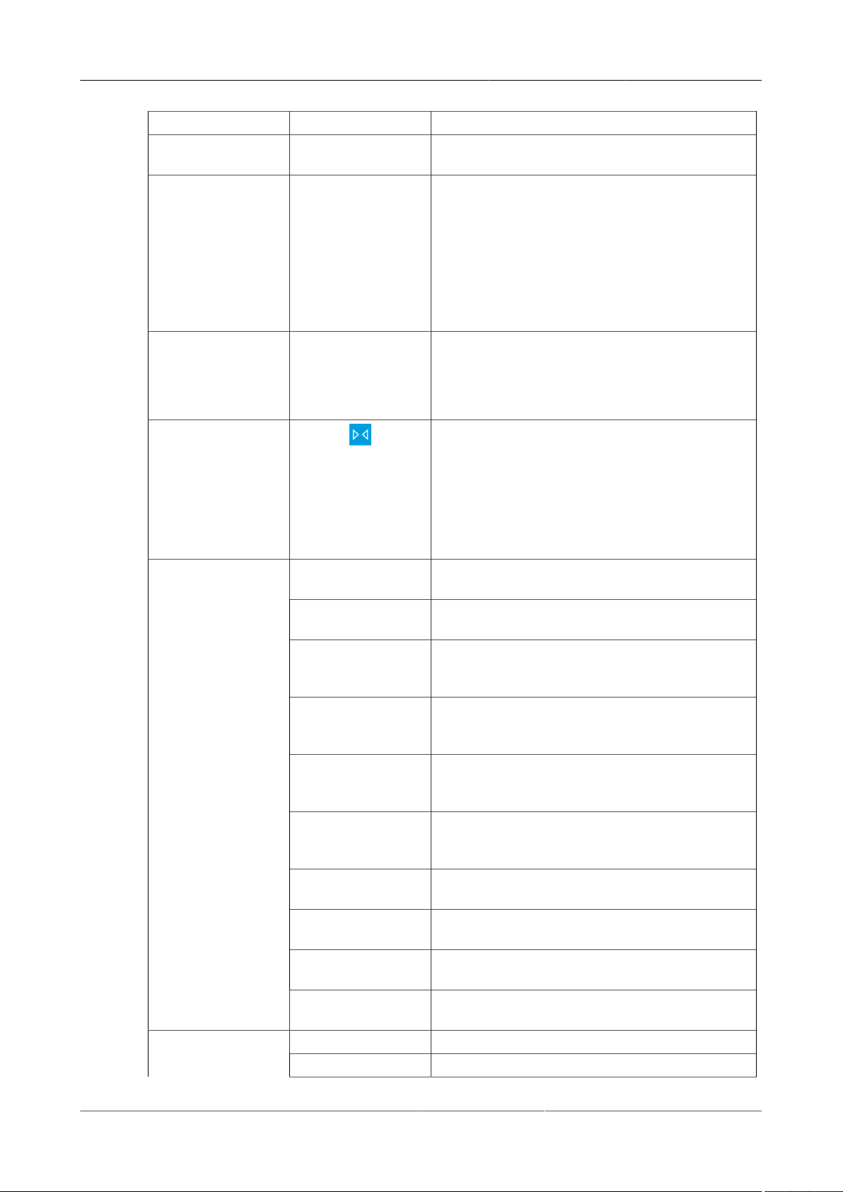
4.2. Lock-in Tab

Control/Tool Option/Range Description Harm 1 to 1023 Multiplies the demodulator's reference frequency

Demod Freq (Hz) 0 to 50 MHz Indicates the frequency used for demodulation

Phase (deg) -180° to 180° Phase shift applied to the reference input of the

Zero Adjust the demodulator phase automatically in

with the integer factor defined by this field.

and for output generation.

The demodulation frequency is calculated with oscillator frequency times the harmonic factor. When the HF2LI-MOD option is used linear combinations of oscillator frequencies including the harmonic factors define the demodulation frequencies.

demodulator.

When the HF2LI-MF option is used, the phase shift is also applied to the Signal Outputs.

order to read zero degrees.

Signal

Shifts the phase of the reference at the input of the demodulator in order to achieve zero phase at the demodulator output. This action maximizes the X output, zeros the Y output, zeros the Θ output, and leaves the R output unchanged.

Sig In 1 Signal Input 1 is connected to the corresponding

demodulator.

Sig In 2 Signal Input 2 is connected to the corresponding

demodulator.

Aux In 1 Auxiliary Input 1 is connected to the

corresponding demodulator. The input bandwidth is limited to 20 kHz.

Aux In 2 Auxiliary Input 2 is connected to the

corresponding demodulator. The input bandwidth is limited to 20 kHz.

DIO D0 DIO D0 is connected to the corresponding

demodulator. The input bandwidth is limited to 2 MHz.

DIO D1 DIO D1 is connected to the corresponding

demodulator. The input bandwidth is limited to 2 MHz.

Aux Out 3 Auxiliary Output 3 is connected to the

corresponding demodulator.

Aux Out 4 Auxiliary Output 4 is connected to the

corresponding demodulator.

Aux In 1 Auxiliary Input 1 is connected to the

corresponding demodulator.

Aux In 2 Auxiliary Input 2 is connected to the

corresponding demodulator. 1 1st order filter 6 dB/octOrder 2 2nd order filter 12 dB/oct

HF2 User Manual - LabOne Edition Revision 34390 Zurich Instruments 97

Page 98

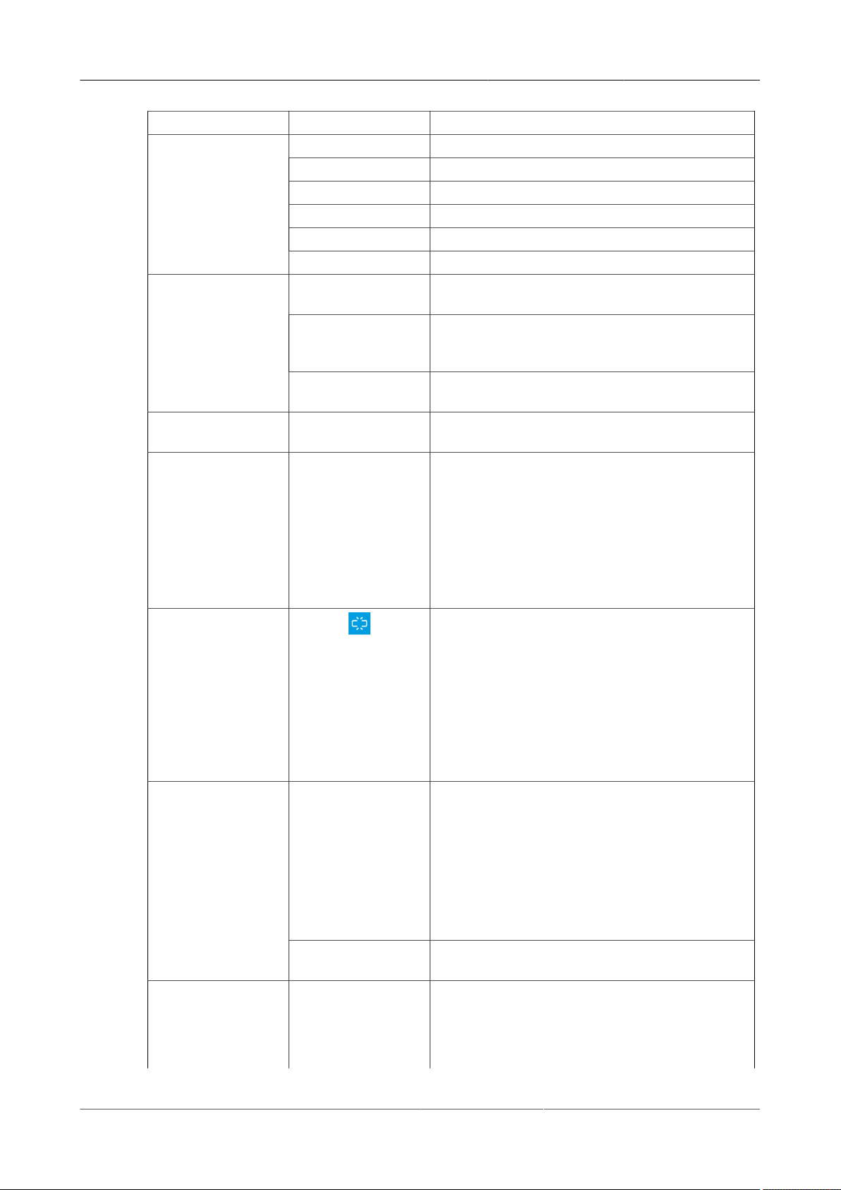
4.2. Lock-in Tab

Control/Tool Option/Range Description

TC/BW Select

TC/BW Value numeric value Defines the low-pass filter characteristic in the

Sinc ON / OFF Enables the sinc filter.

3 3rd order filter 18 dB/oct 4 4th order filter 24 dB/oct 5 5th order filter 30 dB/oct 6 6th order filter 36 dB/oct 7 7th order filter 42 dB/oct 8 8th order filter 48 dB/oct

TC Defines the low-pass filter characteristic using

time constant of the filter.

BW NEP Defines the low-pass filter characteristic using

the noise equivalent power bandwidth of the

filter.

BW 3 dB Defines the low-pass filter characteristic using

the cut-off frequency of the filter.

unit defined above.

When the filter bandwidth is comparable to or

larger than the demodulation frequency, the

demodulator output may contain frequency

components at the frequency of demodulation

and its higher harmonics. The sinc is an

additional filter that attenuates these unwanted

components in the demodulator output.

Lock Makes all demodulators filter settings equal

(order, time constant, bandwidth).

Pressing the lock copies the settings from

demodulator one into the settings of all

demodulators. When the lock is pressed, any

modification to a field is immediately changing

all other settings. Releasing the lock does not

change any setting, and permits to individually

adjust the filter settings for each demodulator.

Enable Streaming

Rate (Sa/s) 0.22 Sa/s to

ON: demodulator

active

OFF: demodulator

inactive

410 kSa/s

Enables the streaming of demodulated samples

in real time to the host computer. The streaming

rate is defined in the field on the right hand side.

As a consequence demodulated samples can

be visualized on the plotter and a corresponding

numeric entry in the numerical tool is activated.

Note: increasing number of active demodulators

increases load on physical connection to the host

computer.

Disables the streaming of demodulated samples

to the host computer.

Defines the demodulator sampling rate, the

number of samples that are sent to the host

computer per second. A rate of about 7-10 higher

as compared to the filter bandwidth usually

provides sufficient aliasing suppression.

HF2 User Manual - LabOne Edition Revision 34390 Zurich Instruments 98

Page 99

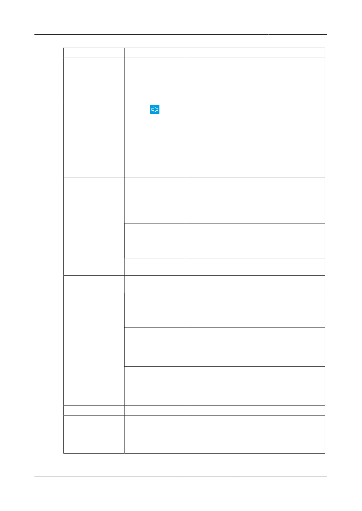
4.2. Lock-in Tab

Control/Tool Option/Range Description

Demodulator Output Rate Lock

Trigger

Trig Mode

Amplitude Unit Vpk, Vrms, dBm Select the unit of the displayed amplitude value. Amp Enable ON / OFF Enables individual output signal amplitude.

This is also the rate of data received by LabOne

Data Server and saved to the computer hard disk.

This setting has no impact on the sample rate on

the auxiliary outputs connectors. Note: the value

inserted by the user may be approximated to the

nearest value supported by the instrument.

Makes all demodulator output rates equal.

Pressing the lock copies the settings from

demodulator one into the settings of all

demodulators. When the lock is pressed, any

modification to a field is immediately changing

all other settings. Releasing the lock does not

change any setting, and permits to individually

adjust the demodulator output rate for each

demodulator.

Continuous Selects continuous data acquisition mode. The

demodulated samples are streamed to the host

computer at the Rate indicated on the left hand

side. In continuous mode the numerical and

plotter tools are continuously receiving and

display new values.

DIO 0 Samples are sent to the host computer

depending on DIO 0 triggering.

DIO 1 Samples are sent to the host computer

depending on DIO 1 triggering.

DIO 0|1 Samples are sent to the host computer

depending on DIO 0 and 1 triggering.

Rising Selects triggered sample acquisition mode on

rising edge of the selected Trigger input.

Falling Selects triggered sample acquisition mode on

falling edge of the selected Trigger input.

Both Selects triggered sample acquisition mode on

both edges of the selected Trigger input.

High Selects continuous sample acquisition mode on

high level of the selected Trigger input. In this

selection, the sample rate field determines the

frequency in which demodulated samples are

sent to the host computer.

Low Selects continuous sample acquisition mode

on low level of the selected Trigger input. In this

selection, the sample rate field determines the

frequency in which demodulated samples are

sent to the host computer.

When the HF2LI-MF option is used, it is possible

to generate signals being the linear combination

of the available demodulator frequencies.

HF2 User Manual - LabOne Edition Revision 34390 Zurich Instruments 99

Page 100

4.2. Lock-in Tab

Control/Tool Option/Range Description On ON / OFF Main switch for the Signal Output corresponding

Range

Add ON / OFF The signal supplied to the add input is added to

Output -range to range Defines the output amplitude for each

to the blue LED indicator on the instrument front

panel.

10 mV Selects output range ±10 mV.

100 mV Selects output range ±100 mV.

1 V Selects output range ±1 V.

10 V Selects output range ±10 V.

the signal output.

demodulator frequency as rms or peak-to-peak

value. A negative amplitude value is equivalent

to a phase change of 180 degree. Demodulator

7 is the signal source for Signal Output 1,

demodulator 8 is the source for Signal Output 2.

HF2 User Manual - LabOne Edition Revision 34390 Zurich Instruments 100

Zurich Instruments HF2 User Manual

Table of Contents

Declaration of Conformity

1.1. Quick Start Guide

1.2. Inspect the Package Contents

1.3. Software Installation

Requirements

Determining the PC Architecture on Microsoft Windows

Windows LabOne Installation

64-bit Windows Installer Issue

Requirements

Linux LabOne Installation

Uninstalling the LabOne Software on Linux

1.4. Handling and Safety Instructions

1.5. Connecting to the Instrument

LabOne Data Server

LabOne Web Server

LabOne API Layer

Device and Settings Dialog

Data Server Connectivity

Available Devices

Saved Settings

Special Settings Files

Messages

Lost Connection to the LabOne Web Server

Reloading...

No Device Discovered

1.6. Troubleshooting

2.1. Features

2.2. Front Panel Tour

2.3. Back Panel Tour

2.4. Ordering Guide

2.5. Operating Modes

3.1. Tutorial HF2LI First Time User

3.2. Tutorial Simple Loop

3.3. Tutorial Dynamic Signals

3.4. Tutorial External Reference

3.5. Tutorial Noise Measurement

3.6. Tutorial Amplitude Modulation

3.7. Tutorial Frequency Modulation

3.8. Tutorial Phase-locked Loop

4.1. User Interface Overview

Plot area elements

Cursors and Math

Tree Sub-Tab

Vertical Axis Groups

4.2. Lock-in Tab

Parameter Table

Block Diagram