Thermo Scientific SOLA II User Manual

SOLA

II

Su lfur Online

User Guide
P/N 90-1307-0

Revision A

B

Analyzer

Part

of

Thermo Fisher Scien

tific

SOLA

II

Su lfur Online

User Guide
P/N 90-1307-0

Revision A

B

Analyzer

© 2017 Thermo Fisher Scientific Inc. All rights reserved.

“Teflon” is a registered trademark of E.I. du Pont de Nemours and Company.
“Watlow” and “EZ-ZONE” are registered trademarks of Watlow Electric Manufacturing Company.
“VICI is a registered trademark of Valco Instruments Co. Inc. and VICI AG.
“Kaowool” is a trademark of Morgan Thermal Ceramics, a business within the Morgan Ceramics Division of the The
Morgan Crucible Company plc.
“Dow Corning” is a registered trademark of Dow Corning Corporation.

All other trademarks are the property of Thermo Fisher Scientific Inc. and its subsidiaries.

Thermo Fisher Scientific (Thermo Fisher) makes every effort to ensure the accuracy and completeness of this manual.
However, we cannot be responsible for errors, omissions, or any loss of data as the result of errors or omissions.
Thermo Fisher reserves the right to make changes to the manual or improvements to the product at any time without
notice.

The material in this manual is proprietary and cannot be reproduced in any form without express written consent
from Thermo Fisher.

Revision History

Revision Level Date Comments

A 02-2004 Initial release.
B 04-2005 Applied standardized formatting, changes to analyzer menu,

stream setup, autocal setup menus; added “At Line Grab
Sample” menu and related items; edited Modbus register for

software v. 1.20.
C 04-2006 Address change.
D 01-2007 Company name change (ECO 5457).
E 04-2007 Revised per ECO 5625.
F 08-2007 Revised per ECO 5921.
G 10-2007 Revised per ECO 6018.
H 03-2008 Revised per ECO 6230.
J 04-2008 Revised per ECO 6320.
K 06-2008 Revised per ECO 6419.
M 04-2009 Revised per ECO 6903.
N 05-2009 Revised per ECO 6915.
P 06-2009 Revised per ECO 6968.
R 04-2010 Revised per ECO 7351.
S 11-2010 Revised per ECO 7578.
T 01-2011 Revised per ECO 7627.
U 04-2011 Revised per ECO 7694.
V 01-2012 Revised per ECO 7897.
W 02-2013 Revised per ECO 8126.
X 01-2014 Revised per ECO 8332.
Y 11-2014 Revised per ECO 8545.
Z 06-2016 Revised per ECO 8659.
AA 06-2016 Revised per ECO 8667.

AB

01-2017

Revised per ECO 8995.

Thermo Fisher Scientific SOLA II User Guide v

Contents

Chapter 1

Chapter 2

Chapter 3

Chapter 4

Safety Information & Guidelines ................................................................... 1-1

Safety Considerations ....................................................................................................... 1-1

Safety Summary ................................................................................................................ 1-2

Safety Operating Information ....................................................................................... 1-2

Electrical Power ................................................................................................................. 1-3

Product Overview ........................................................................................... 2-1

Function ............................................................................................................................... 2-1

Total Sulfur Measurement ............................................................................................ 2-2

Principle of Operation .................................................................................................... 2-4

PUVF Detector .............................................................................................................. 2-5

Pyrolyzer ......................................................................................................................... 2-5

Dryer ................................................................................................................................ 2-6

Mixing Chamber........................................................................................................... 2-6

Injection Valve .............................................................................................................. 2-7

Specifications ..................................................................................................................... 2-8

Parts List ............................................................................................................................2-10

Spare Parts ........................................................................................................................ 2-15

Storage ............................................................................................................................... 2-21

Installation ...................................................................................................... 3-1

Requirements ..................................................................................................................... 3-1

Sample Line Installation ................................................................................................ 3-2

Sample Tubing Preparation.......................................................................................... 3-2

Electrical Connections .................................................................................................... 3-3

DCS & External Connections ....................................................................................... 3-3

Digital Inputs ................................................................................................................ 3-3

Optional Analog Inputs.......................................................................................... 3-4

Analog Outputs ........................................................................................................ 3-5

Other Outputs .......................................................................................................... 3-5

Installation Checklist ....................................................................................................... 3-5

Startup & Shutdown ....................................................................................... 4-1

Initial Startup ..................................................................................................................... 4-1

Startup after Short-Term Shutdown ......................................................................... 4-3

Short-Term Shutdown .................................................................................................. 4-4

Maintenance Shutdown ................................................................................................ 4-4

Emergency Shutdown ..................................................................................................... 4-5

Thermo Fisher Scientific SOLA II User Guide vii

Contents

Chapter 5

Chapter 6

Chapter 7

Chapter 8

Chapter 9

Chapter 10

Operation ........................................................................................................ 5-1

The Interface ...................................................................................................................... 5-1

Begin Analyzing ................................................................................................................ 5-2

Suspending an Analysis ................................................................................................. 5-2

Injection Valve Failure Alarm ...................................................................................... 5-3

Configuration .................................................................................................. 6-1

Analyzer Setup .................................................................................................................. 6-1

Stream Setup.................................................................................................................... 6-4

Clock Setup ...................................................................................................................... 6-6

Modbus Setup ................................................................................................................... 6-7

Dual Range Setup ........................................................................................................... 6-8

Inject Setup ....................................................................................................................... 6-9

Autocal Setup .................................................................................................................. 6-10

Alarms Setup ................................................................................................................... 6-13

Calibration ....................................................................................................................... 6-16

Overview ....................................................................................................................... 6-16

Performing a Low Calibration at Zero* ............................................................. 6-19

Performing a High Calibration ............................................................................. 6-20

The Calibrate High Function ............................................................................ 6-20

The Recalibrate High Function......................................................................... 6-20

Adjusting the Reading .............................................................................................. 6-21

Calibration Setup Menu Items ............................................................................. 6-22

Density Compensation Setup ................................................................................... 6-25

Viewing Alarms ............................................................................................... 7-1

Diagnostics ..................................................................................................... 8-1

Input & Output Test Menu ........................................................................................... 8-1

Set Outputs .................................................................................................................... 8-1

View MUX Analogs ...................................................................................................... 8-2

View 4–20 mA Inputs ................................................................................................ 8-3

View Digital Inputs .................................................................................................... 8-4

View Parameters .............................................................................................................. 8-5

View Com Activity ......................................................................................................... 8-6

Pulse UV Control ............................................................................................................. 8-7

At Line-Grab Sample ...................................................................................... 9-1

Safety Precautions ........................................................................................................... 10-1

Maintenance & Troubleshooting ................................................................. 10-1

Maintenance Schedule .................................................................................................... 10-1

Visual Inspection & Cleaning ...................................................................................... 10-2

Leak Tests ......................................................................................................................... 10-2

viii SOLA II User Guide Thermo Fisher Scientific

Contents

Appendix A

Appendix B

Appendix C

Appendix D

Flow Rate Checks ........................................................................................................... 10-3

The Rotary Valve ........................................................................................................... 10-4

The Mixing Chamber .................................................................................................... 10-4

Replacing the Pyrolyzer Heater ................................................................................. 10-5

The Pyrolyzer Reaction Tube .................................................................................... 10-13

Replacement ............................................................................................................... 10-13

Decoking ...................................................................................................................... 10-15

General Troubleshooting ............................................................................................ 10-15

Contact Information .................................................................................................... 10-19

Warranty ......................................................................................................................... 10-20

Items not Covered under Warranty .................................................................. 10-20

Watlow EZ-ZONE® PM6 Series ..................................................................... A-1

Controller Description ................................................................................................... A-1

Hardware Setup ............................................................................................................... A-1

Display & Keys .................................................................................................................. A-1

Software Configuration ................................................................................................. A-3

Pyrolyzer Settings ....................................................................................................... A-3

Oven Settings ............................................................................................................... A-11

The Lockout Menu ........................................................................................................ A-18

Rotary Valve Service ..................................................................................... B-1

Initial Precautions ............................................................................................................. B-1

Valve Disassembly ........................................................................................................... B-2

Cleaning the Valve Body ............................................................................................... B-3

Cleaning the Rotor ......................................................................................................... B-4

Rotor Assembly ............................................................................................................... B-4

Conditioning Procedure for High Temperature Valves ...................................... B-5

Two-Position Air Actuator O-ring Replacement .................................................. B-6

Disassembly .................................................................................................................. B-6

Replacement ................................................................................................................. B-8

Assembly ........................................................................................................................ B-9

Valve Alignment ............................................................................................................. B-10

Rebuild the Assembly .................................................................................................... B-11

Dinfa Valve Service ....................................................................................... C-1

Overview ............................................................................................................................. C-1

Troubleshooting .............................................................................................................. C-5

TCP/IP Bridge ................................................................................................ D-1

Hardware Configuration ................................................................................................ D-1

Software Configuration ................................................................................................. D-2

The Browser Interface ................................................................................................... D-3

24 Hours Chart ........................................................................................................... D-4

24 Hours Table Format ............................................................................................ D-4

Thermo Fisher Scientific SOLA II User Guide ix

Contents

Appendix E

Appendix F

Appendix G

Appendix H

Appendix I

Appendix J

Configuration ............................................................................................................... D-4

At Line Sample ............................................................................................................ D-8

Version 1.20 Modbus Registers ................................................................... E-1

Coils (0)0001 to (0)0040 ............................................................................................... E-1

Status Inputs (1)0001 to (1)0025 ................................................................................. E-3

Input Registers (3)0001 to (3)0040...........................................................................E-4

Holding Registers (4)0001 to (4)0049 ..................................................................... E-5

The Workstation ............................................................................................. F-1

Installing Workstation Software .................................................................................. F-1

Workstation Operation .................................................................................................. F-3

Statistics .......................................................................................................................... F-5

Density Values & Trend ............................................................................................ F-5

Cal Validation History ................................................................................................ F-5

Stream Plot .................................................................................................................... F-5

Detector Status ............................................................................................................. F-6

Alarms Status ................................................................................................................ F-6

Remote Controls .......................................................................................................... F-7

Analyzer Status ............................................................................................................. F-8

Configuration .................................................................................................................... F-8

The X-Purge System ...................................................................................... G-1

Description......................................................................................................................... G-1

X-Purge Specifications ................................................................................................... G-3

Installation ......................................................................................................................... G-4

AC Power ...................................................................................................................... G-4

Alarm Signal ................................................................................................................. G-5

Startup ............................................................................................................................... G-5

Shutdown .......................................................................................................................... G-6

Power or Purge Loss Shutdown ............................................................................ G-7

Maintenance ..................................................................................................................... G-7

Timer Adjustment .......................................................................................................... G-8

Software Menu Tree ...................................................................................... H-1

PUVF Optical Bench ........................................................................................ I-1

Dual PMT Supply Option ................................................................................ J-1

Overview ............................................................................................................................... J-1

Menu Changes for Dual PMT Supply Option ......................................................... J-2

Calibration Setup .......................................................................................................... J-2

AutoCal Setup ................................................................................................................ J-3

Stream Setup .................................................................................................................. J-3

x SOLA II User Guide Thermo Fisher Scientific

Contents

Appendix K

Appendix L

Appendix M

4–20 mA Range Setup ................................................................................................ J-3

Diagnostics Display ...................................................................................................... J-3

At Line-Grab Sample ................................................................................................... J-4

Installation ........................................................................................................................... J-4

Toxic & Hazardous Substances Tables ....................................................... K-1

Connecting to a Sarasota FD910 Density Meter .......................................... L-1

Purpose ................................................................................................................................ L-1

Connections ........................................................................................................................ L-1

Connecting One Density Meter to a Dual Stream System ............................ L-3

Related Technical Bulletins .......................................................................... M-1

Appendix N

Appendix O

Trace Level Measurements ............................................................................. ..N-1

Vapour Sample Measurements.........................................................................O-1

Thermo Fisher Scientific SOLA II User Guide xi

Chapter 1

Failure to follow appropriate safety procedures or inappropriate use of the
equipment described in this manual can lead to equipment damage or injury
to personnel.

Safety

Considerations

Safety Information & Guidelines

This chapter contains information that must be read and understood by all
persons installing, using, or maintaining this equipment.

Any person working with or on the equipment described in this manual is
required to evaluate all functions and operations for potential safety hazards
before commencing work. Appropriate precautions must be taken as
necessary to prevent potential damage to equipment or injury to personnel.

The information in this manual is designed to aid personnel to correctly and
safely install, operate, and maintain the system described; however, personnel
are still responsible for considering all actions and procedures for potential
hazards or conditions that may not have been anticipated in the written
procedures. If a procedure cannot be performed safely, it must not be

performed until appropriate actions can be taken to ensure the
safety of the equipment and personnel. The procedures in this manual

are not designed to replace or supersede required or common sense safety
practices. All safety warnings listed in any documentation applicable to
equipment and parts used in or with the system described in this manual
must be read and understood prior to working on or with any part of the
system.

Failure to perform the instructions and procedures in this manual
or other documents pertaining to this system correctly can result
in equipment malfunction, equipment damage, and/or injury to
personnel.

Thermo Fisher Scientific SOLA II User Guide 1-1

Safety Information & Guidelines

Safety Summary

Safety Operating

Information

Safety Summary

The following admonitions are used throughout this manual to alert users to
potential hazards or important information. Failure to heed the warnings

and cautions in this manual can lead to injury or equipment
damage.

Warning Warnings notify users of procedures, practices, conditions, etc.

which may result in injury or death if not carefully observed or followed. The
triangular icons with warnings vary depending on the hazard. σ

Caution Cautions notify users of operating procedures, practices, conditions,

etc. which may result in equipment damage if not carefully observed or
followed. σ

Caution Static sensitive component. Appropriate handling precautions

required to prevent damage. σ

Note Notes emphasize important or essential information or a statement of

company policy regarding an operating procedure, practice, condition, etc. σ

This section contains general safety and operating information applicable to
analytical systems, which must be understood by all persons installing, using,
or maintaining the analyzer system. This information is designed to aid
personnel in the safe installation, operation, and service of the analyzer and
sample systems. It is not designed to replace or limit appropriate safety
measures applicable to work performed by personnel. Any additional safety
and operating measures that are required must be determined by and
followed by personnel performing work on the system.

Caution Failure to heed the following information may lead to equipment

damage or injury to personnel. σ

Protective eyewear (glasses with side shields or goggles as appropriate) must
be worn when servicing any part of the analyzer or sample system. When
servicing the sample system, chemical resistant gloves appropriate for the
materials in the system must be worn. When servicing the hot analyzer oven,
internal components (e.g., detectors), or hot sample system components,
appropriate gloves must be worn. Heated components should be allowed to
cool before servicing if possible. Other appropriate equipment or clothing
must be used as required by the type of work performed.

1-2 SOLA II User Guide Thermo Fisher Scientific

Safety Information & Guidelines

Electrical Power

Electrical Power

Caution Ovens, internal components, and sample systems may be hot even

when power is not applied to the unit. Take appropriate precautions to
prevent injury resulting from contact with hot items. σ

All applicable regulations and procedures must be followed for the work
performed. Before beginning any work on the system, carefully consider all
the potential hazards and ensure that appropriate measures are taken to
prevent injury to personnel and damage to equipment.

The system uses AC power at 110 Vac (an optional step-down transformer is
available for 220 Vac). The AC power is converted to DC at several voltage
levels. Appropriate precautions must be taken to prevent sparks present in the
analyzer environment that may ignite combustible materials. Precautions must
also be taken to prevent electrical shock if the analyzer or sample system
enclosures are opened.

The AC power to the system must be free from noise, surges, sags, and spikes
for proper system operation. AC power circuit breakers and wiring must be
sized properly for the required current. All wiring installations must meet
applicable electrical codes.

The fuse is located on the analyzer terminal block.

Caution If it becomes necessary to replace the fuse, it must be replaced with
one of the same rating: Fuse, 3 A S/B (p/n TE-4510). σ

Warning Remove power prior to performing any work internal to the

instrument. An override is available for use in non-hazardous areas; however,
removal of components while the instrument is energized is not permitted. σ

Thermo Fisher Scientific SOLA II User Guide 1-3

Chapter 2

Function

Product Overview

The Thermo Scientific SOLA II sulfur online analyzer combines proven
detection technology, easy-to-use, menu-driven software, and advanced
diagnostics to offer unsurpassed flexibility and reliability. The instrument
offers field programmable ranges, high sensitivity, total sulfur measurement,
fast response time, linearity through all ranges, and low consumables.

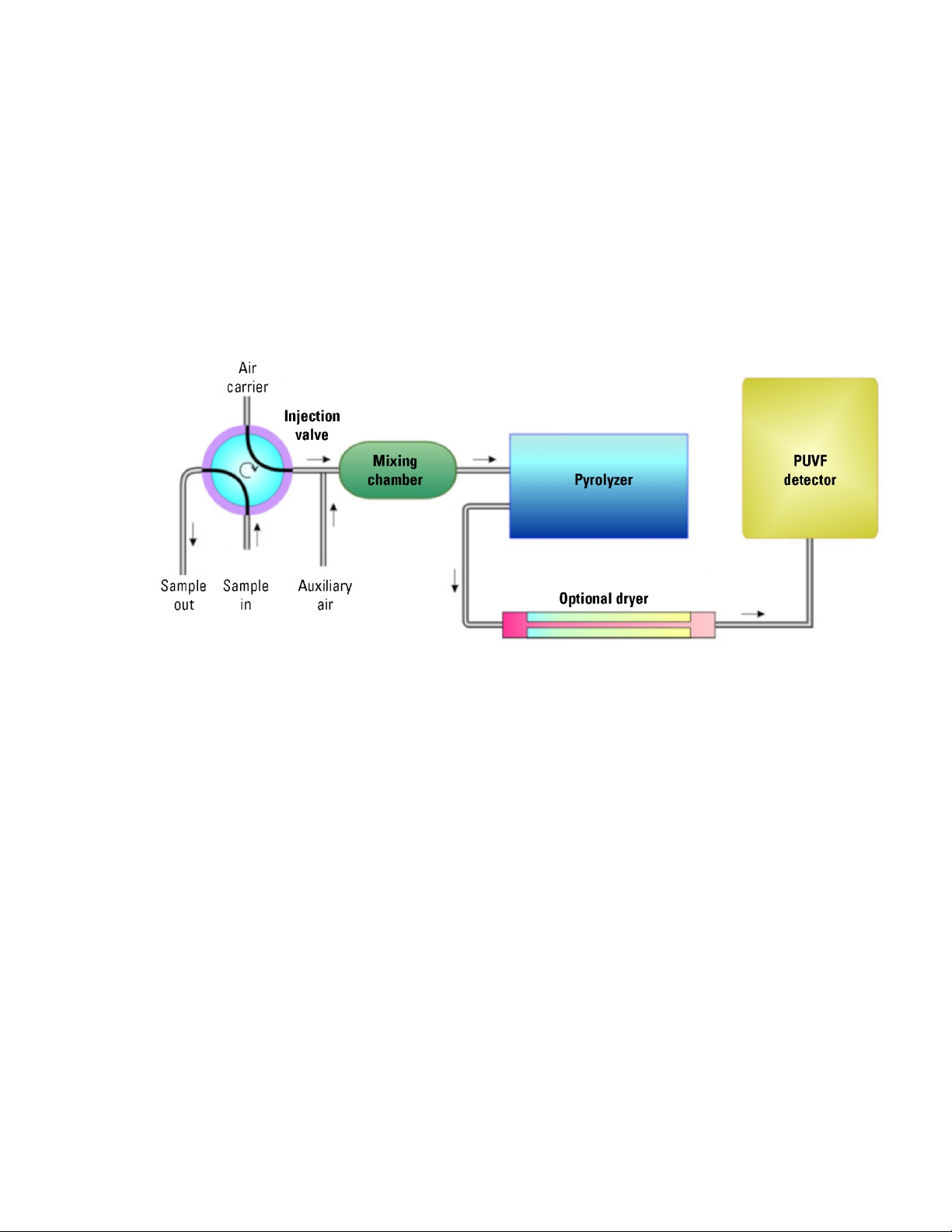
Major components of the SOLA II include a sample injection valve, carrier gas
flow control system, mixing chamber, pyrolyzer, optional dryer, and a pulsed
ultraviolet fluorescence (PUVF) detector. Unlike the original SOLA instrument,
the PUVF is not a subassembly. The SOLA II is a single assembly with one
software program and one user interface.

The sample injection valve periodically transfers a small amount of sample
(approximately 1.0 µL) into an air carrier gas. The air/sample mixture passes
through the mixing chamber to ensure complete mixing and then flows to the
pyrolyzer. The pyrolyzer combusts all sample components to SO2, CO2, and
H2O at approximately 1100°C (2012°F). The optional dryer (application
dependent) removes water from the sample that is produced during
combustion. The PUVF detector accurately measures the amount of SO2
produced during combustion of the sample.

An appropriate sample conditioning system is mandatory for proper
functioning. The sample conditioning system should:

λ Regulate sample pressure and temperature.

λ Provide filtration to at least a 0.5-micron particle size. Staged filtration is

recommended (e.g. going from 10 micron to 5 micron to 0.5 micron). The

final filter should contain a hydrophobic element to remove undissolved

water.

λ Ensure that a representative sample is transported to the analyzer in the

desired time.

λ Maintain the sample in a single phase.

Thermo Fisher Scientific SOLA II User Guide 2-1

Product Overview

Total Sulfur

Measurement

Total Sulfur Measurement

Note Liquid samples with high vapor temperatures such as naphthas and

gasolines will require sample backpressure regulation +0 25–35 psig. σ

λ Remove undissolved water.

Sample should be delivered to the sample conditioning system using a sample
probe. The sample probe should be designed and fabricated so that sample is
extracted from near the center of the process pipe, preventing the
unnecessary introduction of pipe scale and other particulate that tend to
accumulate along the process pipe walls.

Figure 2–1. Functional block diagram

Total sulfur measurement is based upon the precise measurement of the SO2
concentration produced from a wide variety of compounds containing sulfur,
such as H2S, COS, methyl mercaptan, benzothiophenes, dibenzothiophenes,
sulfides, disulfides, and thiols. Consider the measurement of a sample of
diesel, gasoline, or another common petroleum fraction such as naphtha for
liquid phase samples. For liquid phase samples, the analyzer periodically
injects a very small quantity of sample (1.0 µL) of the petroleum fraction into
a hot oven (110°C to 220°C / 230°F to 428°F) where it is vaporized and mixed
with air. Analysis of gas phase samples requires sample sizes of 0.1 to 1.0 cm3.
After thoroughly mixing with air, the sample enters the pyrolyzer, where all
components of the sample are combusted at 1100°C (2012°F) to CO2, H2O, or
SO2. The quantity of SO2 formed during the combustion process is directly
proportional to the total sulfur content of the petroleum fraction.

The analyzer is equipped with a PUVF detector that accurately measures the
quantity of SO2 formed during the combustion process. The SO2 molecules

2-2 SOLA II User Guide Thermo Fisher Scientific

Product Overview

Total Sulfur Measurement

enter the cell of the PUVF detector where they are exposed to ultraviolet (UV)
light. Absorption of UV light by SO2 molecules results in an excited state of
the SO2 molecules. The excited state SO2 molecules exist at a higher energy
state (due to absorption of energy in the form of UV light) and rapidly relax
to their original energy level or ground state through the emission of light.
This process is called fluorescence. The intensity of the light emitted by SO2
fluorescence is directly proportional to the SO2 concentration. Pulsing the UV
light allows more energy (UV light) to be delivered to the sample, increasing
the fluorescence intensity for a given SO2 concentration. This results in
increased overall sensitivity of the instrument.

At the PUVF detector, it is important to ensure that the measured light is
representative of only the SO2 concentration and not some other species. SO2
molecules emit light through fluorescence at a specific wavelength, and the
PUVF detector utilizes bandpass filters to ensure that only light from SO2 is
measured. Once the proper wavelength of light is selected, its intensity is
measure by a photomultiplier tube (PMT). The PMT converts light energy to
electrical energy through manipulation of the photoelectric effect. The
electrical signal generated by the PMT is finally processed by the analyzer
electronics and software to determine and report the concentration of total
sulfur in the liquid petroleum fraction or gas sample.

The analyzer can be configured to report total sulfur in parts per million
(ppm), parts per billion (ppb), or milligrams per liter (mg/L).

λ When using the ppm or ppb units of measure, you can choose to calibrate

the analyzer in terms of ppm (w/w), ppm (v/v), ppm (w/v), ppb (w/w),

ppb (v/v), or ppb (w/v).

λ When using density compensation and the ppm or ppb units are selected,

the display shows ppm/weight or ppb/weight.

Units of concentration calculated on a weight/weight basis are sensitive to
sample density. If the density of the calibration standard is significantly
different from the density of the sample, a density correction should be
applied.

λ If the sample density varies significantly, a density correction is also

necessary when using concentration units of ppm (w/w) or ppb (w/w).

λ If using mg/L, ppm (w/v), ppm (v/v), ppb (w/v), or ppb (v/v), a density

correction is not required.

Thermo Fisher Scientific SOLA II User Guide 2-3

Product Overview

Principle of

Operation

Principle of Operation

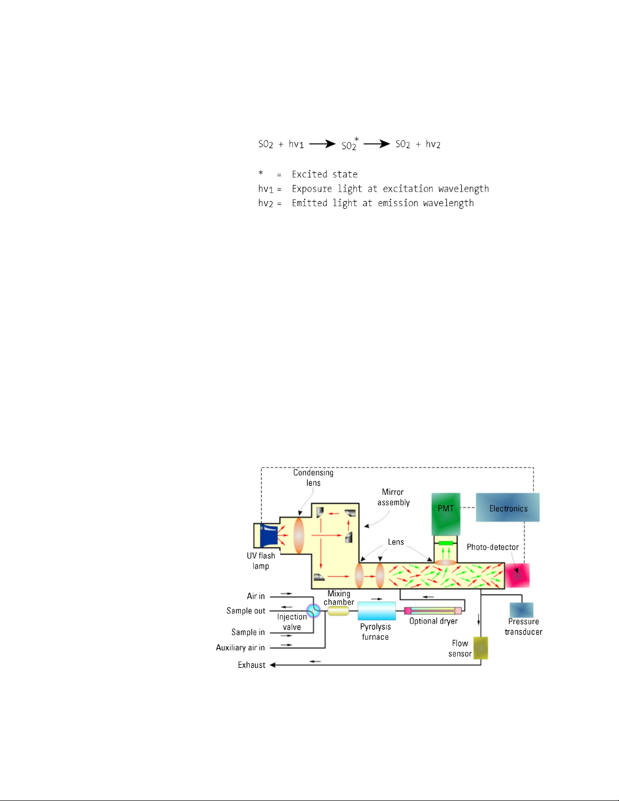
The detector is based on the principle that SO2 molecules absorb UV light and
become excited at one wavelength, then decay to a lower energy state
emitting UV light at a different wavelength. Specifically,

The sample inlet bulkhead draws the sample into the analyzer. The sample is
mixed with air and passes through a pyrolyzer furnace that oxidizes the sulfur
molecules in the sample to produce SO2. The sample then flows into the
fluorescence chamber where pulsating UV light excites the SO2 molecules. The
condensing lens focuses the pulsating UV light onto a mirror assembly. The
mirror assembly contains four selective mirrors that reflect only the
wavelengths that excite SO

molecules.

2

As the excited SO

molecules decay to lower energy states, they emit UV light

2

that is proportional to the total sulfur concentration in the sample. The
bandpass filter allows only the wavelengths emitted by the excited SO

2

molecules to reach the PMT, which detects the UV light emission. The photo
detector, located at the back of the fluorescence chamber, continuously
monitors the pulsating UV light source to provide compensation for
fluctuations in the UV light source. The measured SO

concentration

2

(representing total sulfur in the sample) is processed, displayed on the front
panel display, and sent to the analog outputs.

Figure 2–2. Typical functional flow diagram

2-4 SOLA II User Guide Thermo Fisher Scientific

Product Overview

PUVF Detector

Pyrolyzer

Principle of Operation

The PUVF detector includes and controls the following:

λ UV pulsed light and associated systems

λ Reaction chamber temperature control

λ Digitizing of PMT signal

λ Smoothing of measurement signal using moving average

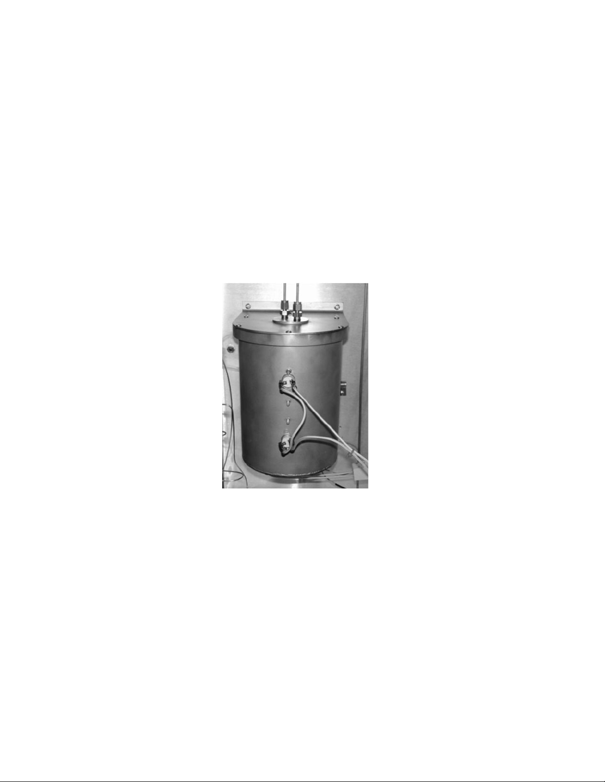
Measuring total sulfur with the PUVF detection method requires the
conversion of all sulfur compounds in the sample to SO2. This is typically
accomplished with the pyrolyzer, an electrically heated furnace designed by
Thermo Fisher Scientific. The pyrolyzer typically operates at a temperature of
1100°C (2012°F) to oxidize sulfur without need for a catalyst.

Figure 2–3. Pyrolyzer

Thermo Fisher Scientific SOLA II User Guide 2-5

Product Overview

Dryer

Mixing Chamber

Principle of Operation

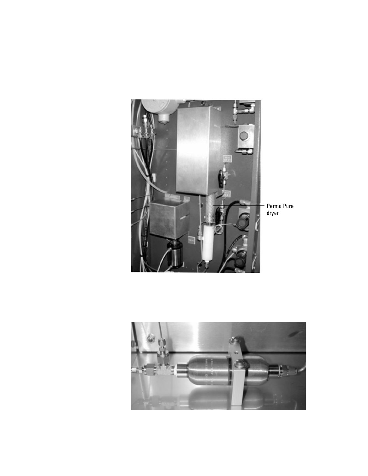
The optional Perma Pure dryer removes moisture from the sample prior to its
entry into the PUVF detector. A filter is positioned before the dryer to protect
it from impurities. Dryer tubing consists of multiple small tubes encased in a
large outer tube. Air circulates through the outer tube with sample passing
through the inner tube. Moisture passes from the sample through the tubing
where it is carried to the condensate drain by the airflow in the outer tube.

Figure 2–4. Optional dryer

The mixing chamber mixes the gases and permits the sample to vaporize to a
gaseous state before entering the pyrolyzer.

Figure 2–5. Typical mixing chamber

2-6 SOLA II User Guide Thermo Fisher Scientific

Product Overview

Injection Valve

Principle of Operation

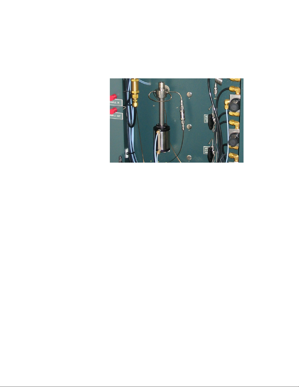
The injection valve periodically injects precisely measured quantities of the
sample stream into a controlled carrier airflow. An auxiliary airflow is added
to this sample and air mixture. The sample then passes to the mixing chamber
where it vaporizes (if necessary) and is thoroughly mixed with the air. See

Appendix B for rotary injection valve service.

Figure 2–6. Injection valve

Thermo Fisher Scientific SOLA II User Guide 2-7

Product Overview

Results may vary under different operating conditions.

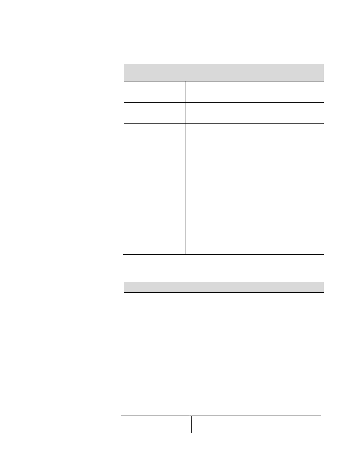
Specifications

Specifications

Table 2–1. Mechanical specifications

Mechanical
specifications

Dimensions, H x W x D 40 x 24 x 18 in (102 x 61 x 46 cm)
Weight Approximately 200 lb (91 kg)
Mounting Wall or rack mount
Ambient temperature 12ºC to 40ºC (54ºF to 104ºF)
Incoming purge air

temperature
Area classification CSA:

12ºC to 40ºC (54ºF to 104ºF)

Class 1, Div. 2, Groups B, C, D, T2, or T3 (T3 optional with
back-up purge system)

Class 1, Div. 1, Groups B, C, D, T2, or T3 (optional, X­Purge system; T3 optional with back-up purge system)

ATEX:

Zone 1, G Ex pxb IIC T Gb (optional, X-Purge system; T3
and T4 optional with back-up purge system)

II 3 G Ex pz IIC T3 Gc, SOLA II Flare or CV. T3 or T4
optional with back-up purge system, standard SOLA II

IECEx:

G Ex pz IIC T Gc (T3 and T4 with back-up purge system)
Zone 1, G Ex px IIC T Gb (X-Purge system); T3 and T4

with back-up purge system)

Table 2–2. Analytical specifications

Analytical specifications

2-8 SOLA II User Guide

Detector Pulsed UV fluorescence with pyrolyzer for total sulfur

measurement

Full scale range Ranges from 0–5 ppm (w/w) to 0–50,000 ppm (w/w)

(consult factory for other ranges).
Unique ranges may be assigned to Streams 1 and 2.
Trace option enables 0–2 ppm (w/w) measuring range

with LDL of 25 ppb (consult factory for other ranges).

Repeatability Calculated at 1 standard deviation

±1% of full scale at 2x injections per minute
±2% of full scale at 1x injection per minute

Standard SOLA II (not Trace level) for full scale ranges of

10ppm or lower, the repeatability is ±2% of full scale at

2x injections per minute.

Equal to repeatability, for ranges >1% full scale, consult

Linearity

factory for linearity specification.

Thermo Fisher Scientific

Product Overview

Specifications

Response time Programmable. Analyzer is semi-continuous; initial response

occurs at each injection

Calibration Automatic or Manual, with ability for Distributed Control

System (DCS) to force an autocal (via contact inputs or
Modbus)

Calibration method External standard(s), 2-point calibration

Table 2–3. Controller specifications

Controller specifications
Display 4-line x 20-character, vacuum fluorescent display, indicating

stream selected, range selected, or off-line

User interface 4 buttons with context-sensitive functions
Streams Dual streams optional with autostream select or DCS control

of stream selection

Alarms Standard: I/O board time-out, oven/pyrolyzer temperature,

valve fault (lamp rate of change), chamber flow, chamber
temperature, lamp voltage, autocal fail, HIGH and HIGH
HIGH concentration

Optional: Sample flow, analog input board time-out

Alarm relays/indicators SPST, 2 A at 240 Vac or 10 A at 24 Vdc; 8 total
Analog signal output Isolated, 4–20 mA; 2 total
Analog signal load ≤ 600 ohms
Inputs Dry contact; remote suspend, remote calibration, remote

range select, remote stream select

I/O ports Standard: RS485 Modbus RTU; RS485/RS232 Modbus

RTU
Optional: TCP/IP encapsulated Modbus, browser-enabled

interface

Thermo Fisher Scientific SOLA II User Guide 2-9

Product Overview

Parts List

Parts List

Table 2–4. Other specifications

Other specifications
AC power Standard: 110 Vac, 50/60 Hz at 2000 W

Optional: 220 Vac, 50/60 Hz

Oven and purge air Instrument air: 55–100 psig, water and oil free; -40ºC (-

40ºF) dew point, particles ≤ 5 m, ISA grade hydrocarbon
free, 8 SCFM (maximum)

Carrier and auxiliary air Zero grade air: 80 psig, 300 sccm (maximum)

Heliox (79% helium, 21% oxygen): 80 psig, 200 sccm
(maximum), for trace option

Sample tubing 316 stainless steel, cleaned and free from oils, moisture,

and debris

Sample wetted components 316 stainless steel, Teflon®, and graphite-filled Teflon;

others application dependent (Kalrez, Viton)

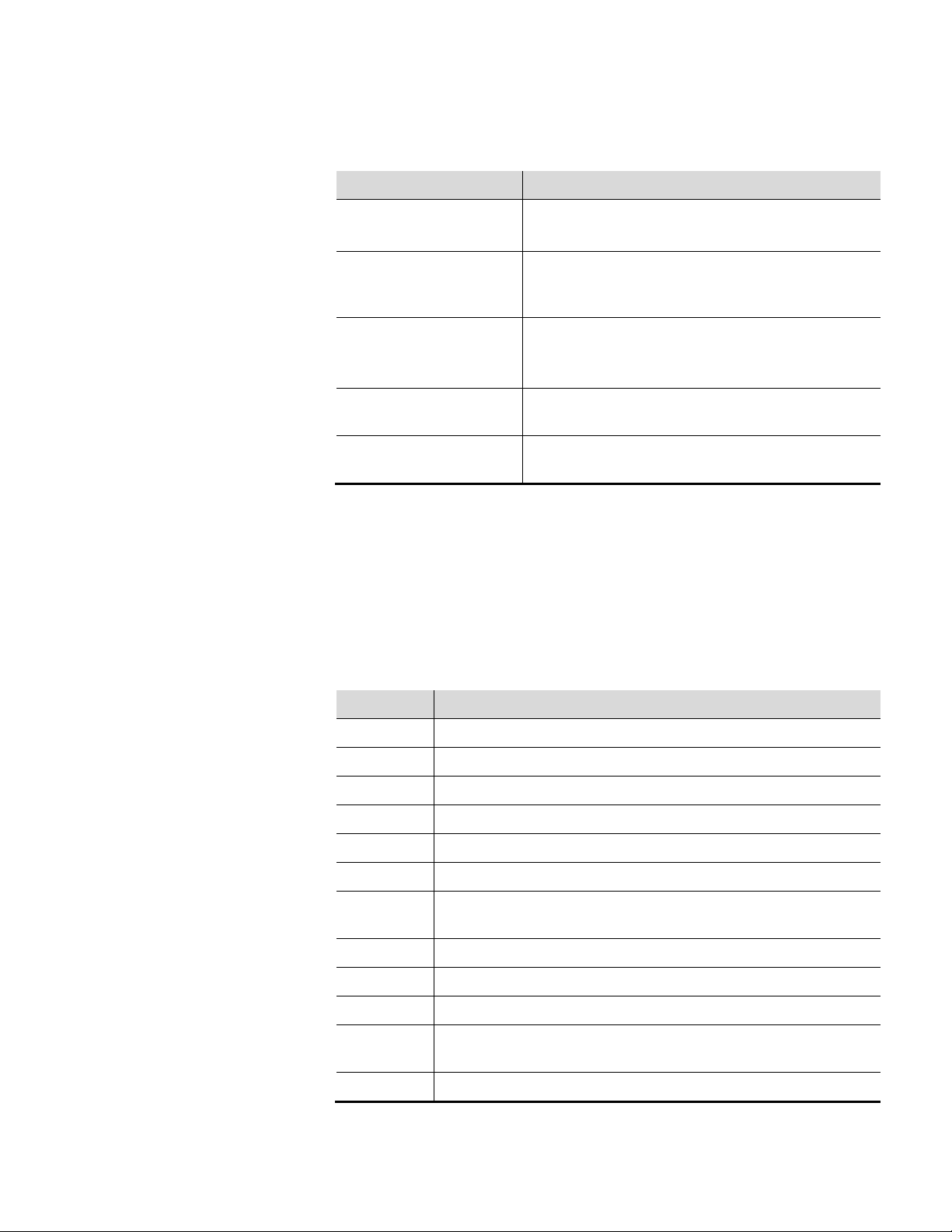
The following table lists the SOLA II / SOLA II Trace parts.

Note Unless otherwise specified, the parts listed below are for the SOLA II

and the SOLA II Trace units. σ

Table 2–5. SOLA II / SOLA II Trace parts list

P/N Description

75-1350-0 Actuator, standard temperature, air, 36 deg, 10-port
75-1348-0 Actuator, standard temperature, air, 90 deg, 6-port
89-2913-0 Assembly, Lookout Software
TE-8812 Attenuator, photo cell
TE-8887 Base assembly, PMT
TE-57P713-1 Bench assembly, SOLA II standard unit
TE-57P7125-1 Bench assembly, SOLA II Trace unit

88-1216-0 Cable, DB9 for RS232 Modbus
TE-6279 Cable, RS232, assembly 6'
88-1217-0 Cable, TCP/IP to CPU
00-1010-S Cal standard for liquid units (specify volume, S concentration, and fluid, i.e.

liter, 6 ppm wt/wt thiophene in #2 diesel)

TE-5365 Connector pins, male, bench

2-10 SOLA II User Guide Thermo Fisher Scientific

Product Overview

P/N Description

TE-4609 Connector, housing, male pin, bench
97-1592-1 Critical operation spare parts kit, Dinfa valve, liquid applications
97-1592-2 Critical operation spare parts kit, Valco valve, gas applications
97-1592-0 Critical operation spare parts kit, Valco valve, liquid applications
TE-8719 Detector filter
TE-8335 Detector lens
TE-8851 Diffuser, photo cell
75-1334-0 Dinfa valve slider 1.2 µl
19-1182-0 Discs, thermal, T 2
19-1183-0 Discs, thermal, T 3
TE-8544 Feet, rubber, shock mounts, optical bench
32-5000 Ferrule, Vespel, graphite, 1/16", for fitting to mixer
TE-8852 Filter, detector

Parts List

HA-100153 Filter, disposable, PUVF inlet, not used with Perm-A-Pure
47-1362-0 Filter, inlet, 2 micron (used for sample and air inlet)
HA-101291 Filter, Perm-A-Pure Dryer
25-1352-0 Flow switch, SS, explosion proof, 1/8” FNPT, SPDT
89-2839-0 Furnace, pyrolyzer, complete assembly
TE-4510 Fuse, 3 amp S/B (PK/5)
18-1579-0 Gauge, 0-100 psi, 1.5 DL, 1/8 CBM
18-1576-0 Gauge, 0-15 psi, 1/5 DL, 1/8 CBM
18-1577-0 Gauge, 0-30 psi, 1/5 DL, 1/8 CBM
HA-101812 Graphite ferrules, reaction tube, furnace
25-6005 Heater, 1000 W, oven
29-1230-0 Heater, fiber insulated, pyrolyzer
64-1301-0 Heater, wire sleeve, flameless burner
TE-9886 Instrument cover
27-1068-0 Key
49-1161-0 Keypad, numeric, 4-position
97-1580-0 Kit, TCP/IP Ethernet, Modbus
97-1403-0 Kit, valve inject
TE-8666 Lamp, xenon, PUVF flash
TE-8892 Lens assembly, detector, complete

Thermo Fisher Scientific SOLA II User Guide 2-11

Product Overview

Parts List

P/N Description

TE-8703 Lens, bi-convex
TE-8333 Lens, condensor
TE-8076 Lens, convex plano-aci
TE-8739 Lens, plano convex- aci
TE-8850 Lens, relay
97-1626-0A Malema flow switch kit
31-1354-0 Manifold assembly, 4-position with solenoid
TE-8888 Mirror assembly, complete, SOLA II standard unit
TE-57P746 Mirror assembly, dual, complete, SOLA II Trace unit
TE-87420 Mirror, entrance
35-1527-0 Mounting bracket, TCP/IP PCB
97-1590-1 One-year spare parts kit, Dinfa valve, liquid phase applications
97-1590-2 One-year spare parts kit, Valco valve, gas phase applications
97-1590-0 One-year spare parts kit, Valco valve, liquid phase applications
TE-4811 O-ring
TE-4808 O-ring (between reaction chamber)
63-1150-0 O-ring kit, Dinfa valve actuator
63-1143-0 O-ring kit, low temperature for Valco valve actuator
TE-4829 O-ring, chamber entrance
TE-4831 O-ring, detector filter
TE-4820 O-ring, lens relay
TE-4830 O-ring, photo cell
TE-4808 O-ring, photo cell conic
63-1135-0 O-ring, pyrolyzer furnace
89-2896-0 PCB, 4-20 mA input
TE-8943 PCB, A/D
TE-8884 PCB, flasher intensity (photo detector)
TE-9681 PCB, flasher supply
TE-8951 PCB, input, PM T signal
89-2899-0 PCB, Modbus RS485, dual channel
TE-9829 PCB, motherboard
55-1228-0 PCB, Netburner TCP/IP Ethernet 10/100
TE-8949 PCB, PUVF DC power supply

2-12 SOLA II User Guide Thermo Fisher Scientific

Product Overview

P/N Description

TE-8765 PCB, PUVF temperature control
89-2897-0 PCB, CPU
89-2803-0 PCB, stream relay
89-2898-0 PCB, digital I/O
TE-8684 Plate, filter lens
TE-8868 PMT, SOLA II standard unit
TE-8391 PMT, SOLA II Trace unit
TE-8165 Power cord, 115 V
85-1173-0 Power supply, 110/220 Vac +5 V, ±12 V, for PCB, input option
85-1164-0 Power supply, 24 VDC , DIN rail mount
TE-9901 Power supply, PMT
32-0024 Reducing union, 316 SS 1/8 tube x 1/16 tube
14-1435-0 Regulator, pressure, 0-100 psi, SS case

Parts List

30-2009 Regulator, pressure, 0-25 psi, 4-way mini
HA-100645 Relay, solid state
25-1001 RTD, used for oven heater
TE-8869 Socket assembly, PMT
97-1646-0 Quick repair kit
97-1644-0 N2, addition, field installation
97-1651-0 Solenoid manifold adapter kit
31-0030 Solenoid, 24 Vdc, 5-port, 4-way, 2-position, manifold mount
31-1367-0 Solenoid, 24 Vdc, 5-port, 4-way, 2-position, manifold mount
97-1589-1 Startup spare parts kit, Dinfa valve, liquid phase applications
97-1589-2 Startup spare parts kit, Valco valve, gas phase applications
97-1589-0 Startup spare parts kit, Valco valve, liquid phase applications
25-1189-0 Switch, differential pressure, 0.2 inH2O
25-1137-0 Switch, pressure sensor, 0-15 psi adj, oven and burner
68-2139-2 Tee, 1/4" x 1/8", Sulfinert
68-2138-2 Tee, 1/8", Sulfinert
89-2650-G Temperature controller, furnace, Watlow, complete Centalac
89-2089-G Temperature controller, oven, Watlow, complete Centalac
29-1113-0 Temperature controller, Watlow
56-1150-0 Terminal block, two pole, ceramic, SS connectors

Thermo Fisher Scientific SOLA II User Guide 2-13

Product Overview

Parts List

P/N Description

5382 Thermistor IM-1002-A5
27-1108-0 Thermocouple, S type
TE-9934 Transducer, flow
TE-9877 Transducer, pressure assembly
TE-8774 Trigger pak for SOLA II bench, standard unit
TE-8392 Trigger pak for SOLA II bench, Trace unit
30-1025-0 Tube, quartz pyrolyzer furnace, looped
64-1304-0 Tubing, 1/16”, Sulfinert
64-1051-0 Tubing, 1/16" OD x 0.02” ID SS
40-0614 Tubing, 1/16" OD x 0.01" ID, SS, capillary
64-1305-0 Tubing, 1/4", Sulfinert
64-1303-0 Tubing, 1/8”, Sulfinert
40-0611 Tubing, black nylon, 1/4" OD x 0.035” wall
40-0609 Tubing, FEP, 0.125” OD x 0.062” ID, high temperature
40-0600 Tubing,1/8” OD x 0.085” ID, 0.020, 304SS
97-1591-1 Two-year spare parts kit, Dinfa valve, liquid phase applications
97-1591-2 Two-year spare parts kit, Valco valve, gas phase applications
97-1591-0 Two-year spare parts kit, Valco valve, liquid phase applications
75-1343-0 Valve head, Valco, 10-port
75-1333-0 Valve head, Valco, 6-port
45-1837-0 Valve, 3-way, air operated
75-1335-0 Valve, Dinfa, 8-port, 1.2 µl, complete assembly
45-1823-0 Valve, Valco rotor 1.0 µl, 6-port
45-1835-0 Valve, Valco rotor, 10-port
75-1340-0 Valve, Valco, 10-port, complete assembly
75-1332-0 Valve, Valco, 6-port, 1µl, complete assembly with rotor
45-1235-0 Valve, 3-way ball, tube to tube, 316SS, TFE seat, 1/8” port size

2-14 SOLA II User Guide Thermo Fisher Scientific

Product Overview

Spare Parts

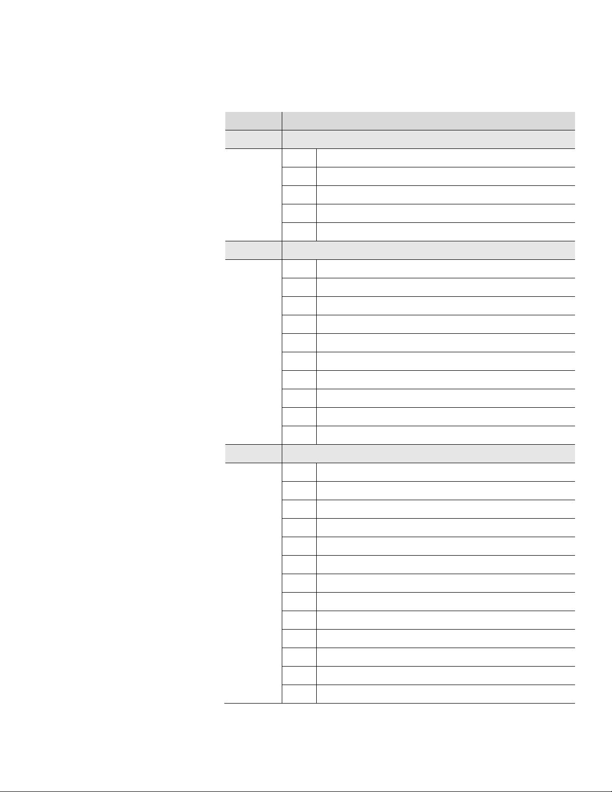
Table 2–6. SOLA II spare part kits

P/N Description
97-1589-0 Startup spare parts kit, Valco valve, liquid phase applications

Qty. Includes
4 Ferrules for pyrolyzer tube fittings, graphite
2 Pyrolyzer tube, looped
2 Pyrolyzer, O-ring 5 5/8” ID x 5 7/8” OD, 1/8” width
2 Rotor, liquid sample valve, 1.0 µl, 4-port or 6-port

97-1590-0 One-year spare parts kit, Valco valve, liquid phase applications

Qty. Includes
1 Heater for pyrolyzer assembly
4 Ferrules for pyrolyzer tube fittings, graphite
2 Pyrolyzer tube, looped

Spare Parts

2 Pyrolyzer, O-ring 5 5/8” ID x 5 7/8” OD, 1/8” width
1 Thermocouple, pyrolyzer S type
4 Rotor, liquid sample valve, 1.0 µl, 4-port or 6-port
1 O-ring kit for liquid injection valve actuator
1 Filter, inline, 2 micron, 1/8” tube
1 Filter, inline, 0.5 micron, 1/8” tube

97-1591-0 Two-year spare parts kit, Valco valve, liquid phase applications

Qty. Includes
2 Heater for pyrolyzer assembly
8 Ferrules for pyrolyzer tube fittings, graphite
3 Pyrolyzer tube, looped
4 Pyrolyzer, O-ring 5 5/8” ID x 5 7/8” OD, 1/8” width
1 Filter, inline 2 micron, 1/8” tube connections
1 Thermocouple, pyrolyzer S type
1 6-port liquid valve head with internal sample loop
8 Rotor, liquid sample valve, 1.0 µl, 4-port or 6-port
2 O-ring kit for liquid injection valve actuator
1 UV flash lamp
2 Filter, inline 0.5 micron, 1/8” tube
1 Injection valve assembly, complete

Thermo Fisher Scientific SOLA II User Guide 2-15

Product Overview

Spare Parts

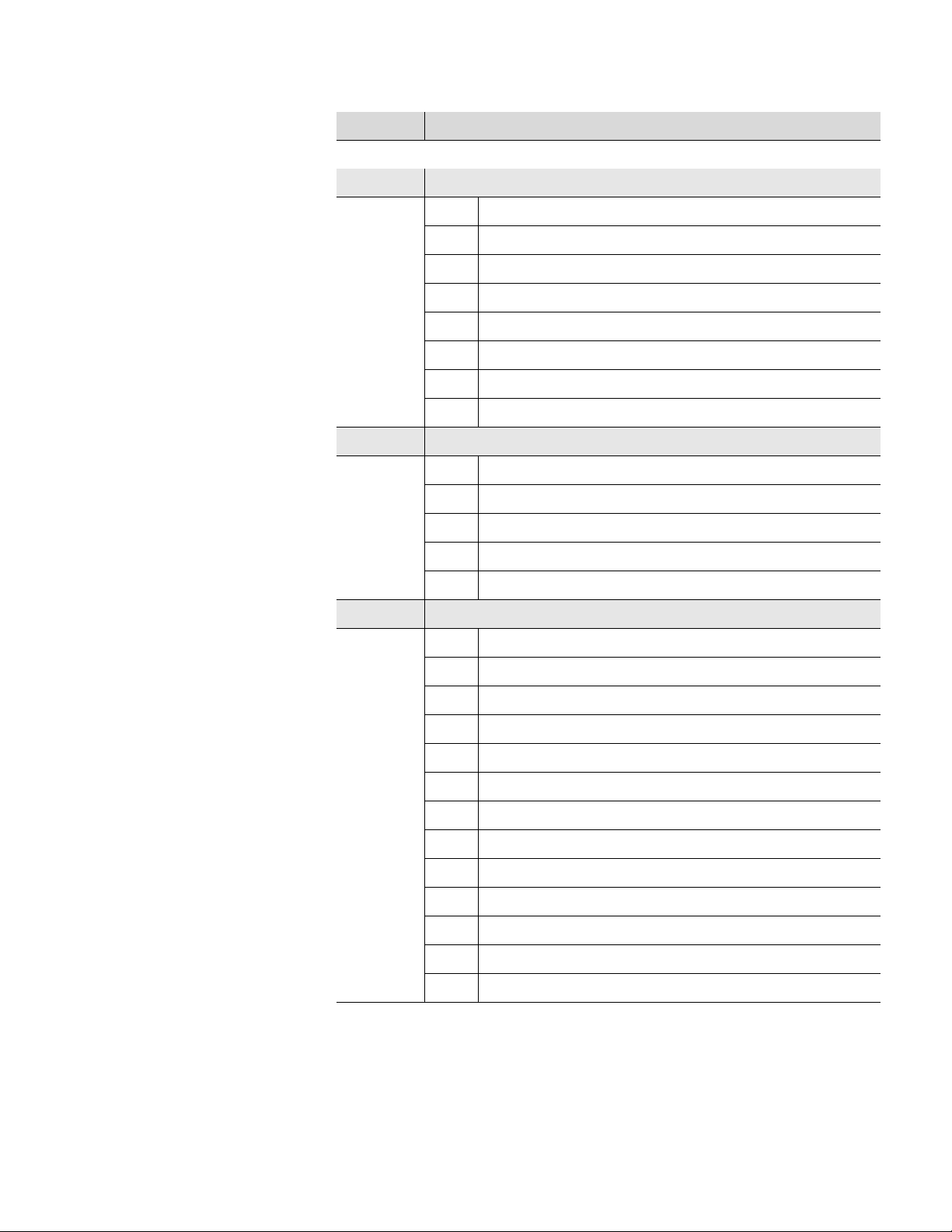
P/N Description

97-1592-0 Critical operation spare parts kit, Valco valve, liquid phase applications

Qty. Includes
1 Optical bench assembly
1 Valve, complete 6-port for liquid
1 Pyrolyzer asse mbly
1 Power supply board for SO2 bench
1 Trigger pak
1 Flasher supply board
1 I/O PCB

97-1589-2 Startup spare parts kit, Valco valve, gas phase applications

Qty. Includes
4 Ferrules for pyrolyzer tube fittings, graphite
2 Pyrolyzer tube, looped
2 Pyrolyzer, O-ring 5 5/8” ID x 5 7/8” OD, 1/8” width
2 Rotor, 10-port, gas

97-1591-2 Two-year spare parts kit, Valco valve, gas phase applications

Qty. Includes
2 Heater for pyrolyzer assembly
8 Ferrules for pyrolyzer tube fittings, graphite
3 Pyrolyzer tube, looped
4 Pyrolyzer, O-ring 5 5/8” ID x 5 7/8” OD, 1/8” width
1 Filter, inline, 2 micron, 1/8” tube connections
1 Thermocouple, pyrolyzer S type
1 10-port valve head, gas
4 Rotor, 10-port, gas
2 O-ring kit for liquid injection valve actuator
1 UV flash lamp
2 Filter, inline, 0.5 micron, 1/8” tube
1 Valve, complete 10-port for gas

2-16 SOLA II User Guide Thermo Fisher Scientific

Product Overview

Spare Parts

P/N Description

97-1592-2 Critical operation spare parts kit, Valco valve, gas phase applications

Qty. Includes
1 Optical bench assembly
1 Valve, complete 10-port for gas
1 Pyrolyzer asse mbly
1 Power supply board for SO2 bench
1 Flash intensity board assembly
1 I/O PCB
1 Trigger pack
1 Flasher supply board

97-1589-1 Startup spare parts kit, Dinfa valve, liquid phase applications

Qty. Includes
4 Ferrules for pyrolyzer tube fittings, graphite
2 Pyrolyzer tube, looped
2 Pyrolyzer, O-ring 5 5/8” ID x 5 7/8” OD, 1/8” width
1 Slider block, 1.2 µl

97-1590-1 One-year spare parts kit, Dinfa valve, liquid phase applications

Qty. Includes
1 Heater for pyrolyzer assembly
4 Ferrules for pyrolyzer tube fittings, graphite
2 Pyrolyzer tube, looped
2 Pyrolyzer, O-ring 5 5/8” ID x 5 7/8” OD, 1/8” width
1 Thermocouple, pyrolyzer S type
1 Slider block, 1.2 µl
1 Filter, inline, 2 micron, 1/8” tube
1 Filter, inline, 0.5 micron, 1/8” tube

Thermo Fisher Scientific SOLA II User Guide 2-17

Product Overview

Spare Parts

97-1591-1 Two-year spare parts kit, Dinfa valve, liquid phase applications

Qty. Includes
2 Heater for pyrolyzer assembly
8 Ferrules for pyrolyzer tube fittings, graphite
3 Pyrolyzer tube, looped
4 Pyrolyzer, O-ring 5 5/8” ID x 5 7/8” OD, 1/8” width
1 Filter, inline, 2 micron, 1/8” tube connections
1 Thermocouple, pyrolyzer S type

97-1591-1 Two-year spare parts kit, Dinfa valve, liquid phase applications

1 Slider block, 1.2 µl
1 UV flash lamp
2 Filter, inline, 0.5 micron, 1/8” tube

97-1592-1 Critical operation spare parts kit, Dinfa valve, liquid phase applications

Qty. Includes
1 Solenoid relay PCB
1 Valve, complete 8-port, 1.2 µl
1 Optical bench assembly
1 Pyrolyzer asse mbly
1 Power supply board for SO2 bench
1 Trigger pak
1 Flasher supply board
1 I/O PCB

2-18 SOLA II User Guide Thermo Fisher Scientific

Product Overview

Spare Parts

Table 2–7. SOLA II Trace spare parts kits

97-1592-3 Critical operation spare parts kit, Valco valve, liquid phase applications

Qty. Includes
1 Valve, inject, 1/16 6-port 1µl, 150 psi, 175°C
1 Optical bench assembly
1 Trigger pak, for SO2 bench
1 Pyrolyzer assembly
1 Board, power supply for SO2 bench
1 Board, flasher supply for SO2 bench
1 PCA, SOLA II I/O circuit PCBA

97-1592-4 Critical operation spare parts kit, Valco valve, gas phase applications

Qty. Includes
1 Valve, 10-port, 1/16”, 150 psi, 175°C
1 Optical bench assembly
1 Trigger pak, for SO2 bench
1 Pyrolyzer assembly
1 Board, power supply for SO2 bench
1 Board, flasher supply for SO2 bench
1 PCA, SOLA II I/O circuit PCBA

Table 2–8. Valco injection valve replacement parts

P/N Description

89-2803-0 Solenoid relay PCB
29-1230-0 Heater for pyrolyzer assembly
HA-101812 Ferrules for pyrolyzer tube fittings, graphite
30-1025-0 Pyrolyzer tube, looped
63-1135-0 Pyrolyzer chamber O-ring seal
47-1362-0 Inline micron filter for orifice flow
27-1108-0 Thermocouple
75-1332-0 Injection valve assembly, 6-port, 1.0 µl
75-1333-0 Injection valve head
45-1823-0 Injection valve rotor, 1.0 µl
63-1143-0 Injection valve O-rings (actuator, low temperature)
TE-9934 Flow transducer assembly

Thermo Fisher Scientific SOLA II User Guide 2-19

Product Overview

Spare Parts

P/N Description

TE-8868 PUVF PMT
TE-8943 A/D PCB
TE-8949 PUVF DC power supply board
TE-8774 PUVF lamp trigger pak (consult factory for SOLA II Trace)
TE-8884 PUVF flash intensity board (consult factory for SOLA II Trace)
TE-9681 Flasher supply board (consult factory for SOLA II Trace)
TE-8951 Input board
TE-8765 PUVF temperature control board
TE-8666 PUVF flash lamp
89-2897-0 CPU
89-2898-0 I/O PCB
85-1164-0 Power supply, 24 Vdc, DIN rail mount

Table 2–9. Dinfa injection valve replacement parts

P/N Description

89-2803-0 Solenoid relay PCB
29-1230-0 Heater for pyrolyzer assembly
HA-101812 Ferrules for pyrolyzer tube fittings, graphite
30-1025-0 Pyrolyzer tube, looped
63-1135-0 Pyrolyzer chamber O-ring seal
47-1362-0 Inline micron filter for orifice flow
27-1108-0 Thermocouple
75-1335-0 Injection valve assembly, 8-port, 1.2 µl
75-1334-0 Injection valve slider, 1.2 µl
TE-9934 Flow transducer assembly
TE-8868 PUVF PMT
TE-8943 A/D PCB
TE-8949 PUVF DC power supply board
TE-8774 PUVF lamp trigger pak (consult factory for SOLA II Trace)
TE-8884 PUVF flash intensity board (consult factory for SOLA II Trace)
TE-9681 Flasher supply board (consult factory for SOLA II Trace)
TE-8951 Input board
TE-8765 PUVF temperature control board

2-20 SOLA II User Guide Thermo Fisher Scientific

Product Overview

Storage

Storage

P/N Description

TE-8666 PUVF flash lamp
89-2897-0 CPU
89-2898-0 I/O PCB
85-1164-0 Power supply, 24 Vdc, DIN rail mount

If storing the instrument, the storage environment should be protected and
free from extremes of temperatures and high humidity.

Thermo Fisher Scientific SOLA II User Guide 2-21

Chapter 3

Requirements

Installation

λ Material and power: Consult the specifications for information required

for installation.

λ Operating environment: For optimum reliability and equipment life, we

recommend that the analyzer be installed in a location protected from

extremes in temperature and weather. The analyzer operates best in a

controlled environment. Ambient temperature and purge air must not

exceed the limits listed in the specifications.

λ Mounting requirements: The mounting site must be as close as possible to

the sampling point. The analyzer must be sheltered from extreme weather

conditions. Avoid mounting the analyzer in high vibration areas. Mount

the analyzer in an accessible location.

λ Cable glands used to supply electrical power must be IP40 rated metallic

cable glands.

λ Blanking elements or plugs used shall be in accordance with national

standards.

Caution This product is extremely heavy. Care must be taken at all times to

avoid injury. Never attempt to move this product alone or without the use of
lift gear. When handling the analyzer, ensure that all four corners are
supported.

σ

Thermo Fisher Scientific SOLA II User Guide 3-1

Installation

Sample Line

Installation

Sample Tubing

Preparation

Sample Line Installation

Note Pressure buildup or liquid accumulation in the analyzer vents degrades

performance. Vent lines must be as short as possible and routed in a manner
that prevents accumulation of liquids. σ

There must be no back pressure on the vent or drain lines. All vents must be
referenced to atmospheric pressure. If the analyzer is installed in a pressurized
analyzer shelter, route all vents from the purge controllers and the PUVF
detector to the exterior of the shelter. All sample lines must be as short as
possible. Sample lines must use new 316 stainless steel that has been prepared
as described in the following section “Sample Tubing Preparation.”

The analyzer will produce erratic readings if backpressure is created or varied
by an obstructed or improperly routed vent.

Review the following cautions prior to performing this procedure.

Caution Isopropyl alcohol is extremely flammable, hazardous if breathed, and

dries skin on contact. When using isopropyl alcohol, avoid breathing the
vapors and contact with the skin. Appropriate measures must be taken to
prevent ignition of the isopropyl alcohol vapors. Use isopropyl alcohol only
where there is adequate ventilation and no ignition sources are present. Refer
to a Material Safety Data Sheet (MSDS) for isopropyl alcohol for additional
important information. σ

Caution Acetone is extremely flammable, hazardous if breathed, and dries

skin on contact. When using acetone, avoid breathing the vapors and contact
with the skin. Appropriate measures must be taken to prevent the acetone
vapors from igniting. Use acetone only where there is adequate ventilation and
no ignition sources are present. Refer to a MSDS for acetone for additional
important information. σ

Caution Acetone dissolves many plastics. Use caution to prevent the acetone

from contacting materials that may be marred or damaged. σ

Caution Take necessary precautions to prevent exposure to hazardous

materials when conditioning the sample tubing with sample. σ

Proper preparation of sample tubing prior to installation is very important.
Prepare the sample tubing as follows.

3-2 SOLA II User Guide Thermo Fisher Scientific

Installation

Power source specification:

Power wiring specification:

Electrical

Connections

DCS & External

Connections

Digital Inputs

Electrical Connections

1. Thoroughly rinse the tubing inside with isopropyl alcohol (isopropanol) or

acetone to remove any oils that may be present.

2. Flush the inside of the tubing with deionized water.

3. Rinse the inside of the tubing again with isopropyl alcohol (isopropanol)

or acetone.

4. Thoroughly blow-dry the tubing with clean air (free of oil and moisture).

Refer to the following AC power information and wire information when
planning and connecting power for the analyzer.

power wire rated for at least 600 Vac and 20 A at the required length.

Warning This apparatus must be earth grounded! σ

Warning Installation of this instrument requires an external, lockable

electrical power isolation switch supplied by the customer. σ

If the optional X-Purge unit is installed, refer to Appendix G for important
installation and operation information.

Wiring to the relay contacts should be sized according to the load imposed by
the alarm systems installed by the user. Maximum current capability of the
alarm contacts is 2 A at 240 Vac or 10 A at 24 Vdc. Voltage is not supplied to
the relay contacts by the analyzer.

110 or 220 Vac, 50/60 Hz, 2000 W

Use stranded, 3-wire copper or tin-plated copper

The following inputs and outputs can be connected to a Distributed Control
System (DCS) or other devices as desired.

Thermo Fisher Scientific SOLA II User Guide 3-3

Installation

Optional Analog Inputs

DCS & External Connections

The following inputs are available for controlling the analyzer from a DCS or
other external source. Refer to the wiring diagrams shipped with your
instrument.

λ Remote Stream Control: A manual switch or DCS output signal can be

used to select the following stream operation when the multiple stream
option is installed. For this control to function, enable the Remote Control
function the Analyzer Setup parameters (Chapter 6).

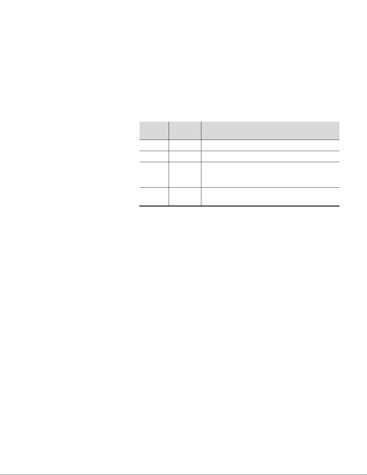
Table 3–1.

Stream
Select 0

Close* Open Analyzes only stream 1
Open Close* Analyzes only stream 2
Close* Close* Analyzer alternates between stream 1 and stream 2 at the

Open Open Analyzer operation for streams is performed as specified in

*Close = Shorted to associated ground terminal

λ Remote Measurement Range Control: To switch to high measurement

Stream
Select 1

Action

time intervals specified in the Stream 1 Dwell Time and

Stream 2 Dwell Time parameters (Chapter 6)

the Stream Setup parameters (Chapter 6)

range, short the Remote Range connection to the Remote Range common
terminal. To switch to low measurement range, open the connection
across the Remote Suspend connectors. The Remote Control function
must be enabled (“Analyzer Setup”, Chapter 6).

λ Remote:

Autocal/Validation: The Autocal/Validation function can be initiated by
closing the contact.

Remote Suspend: To suspend analysis, short the Remote Suspend
connection to the Remote Suspend common terminal. To restart analysis,
open the connection across the Remote Suspend connectors. The Remote

Control function must be enabled (“Analyzer Setup”, Chapter 6).

Analog inputs are available for connecting densitometers used to correct each
stream measurement based on the density of the sample.

3-4 SOLA II User Guide Thermo Fisher Scientific

Installation

Analog Outputs

Other Outputs

Installation

Checklist

Installation Checklist

λ Density Input Stream 1: This 4–20 mA DC input signal represents the

density of the Stream 1 sample. The measured densities at 4 mA and at 20

mA can be programmed into the analyzer using the Density

Compensation Setup menu (Chapter 6).

Density Input Stream 2: This 4–20 mA DC input signal represents the density

of the Stream 2 sample. The measured densities at 4 mA and at 20 mA

can be programmed into the analyzer using the Density Compensation

Setup menu (Chapter 6).

The following outputs are available with the analyzer. Refer to the wiring
diagrams shipped with your instrument for wiring details.

λ Analog Output 1: This 4–20 mA DC signal represents the measured

concentration of Stream 1. The zero value (4 mA DC) represents zero

measured concentration in the sample. Full scale (20 mA DC) represents

the measured concentration specified in High Range or Low Range

(depending on range selected).

λ Analog Output 2: This 4-20 mA DC signal represents the measured

concentration of Stream 2. It is available only if the dual-stream option is

installed. The zero value (4 mA DC) represents zero measured

concentration in the sample. Full scale (20 mA DC) represents the

measured concentration specified in High Range or Low Range

(depending on range selected).

The following outputs are also provided: High/High Alarm Relay, High Alarm
Relay, Off Line Status Relay (fail-safe), Malfunction Alarm Relay (fail-safe,
normally closed), Range Selected, Stream Selected, Purge Alarm (fail-safe).

The following checklist may be copied for use during system installation.
Details for the installation and various specification requirements are
contained in this manual, application specific drawings, and information
supplied with the instrument.

Thermo Fisher Scientific SOLA II User Guide 3-5

Installation

Installation Checklist

NOT

Installation Checklist

Materials used meet specifications defined in Chapter 2.

Operating environment meets requirements defined in Chapter 3.

Mounting meets requirements defined in Chapter 3.

Analyzer condition inspected as follows:

No physical damage, broken parts, or observable defects.

All electronic boards are securely seated.

All cables and wiring connectors are in place and fully seated.

No loose parts (wires, nuts, screws, cables, debris, etc.).

All tubing is properly connected and fittings are tight.

Installation and flow connections adhere to the following:

Sample system properly designed to condition (control pressure, flow, temperature, and particulate)

sample as required by system.

Sample system fast loop panel is installed as close as possible to analyzer for fastest response time.

System gases meet quality and quantity (pressure and flow) specifications according to Chapter 2.

PUVF vent is vented to atmospheric pressure.

PUVF vent is

Inject purge vent will contain instrument air plus 5–10 cm

connected to headers with varying pressure or that may accumulate liquids.

3

of hydrocarbon liquid or gas during suspension
of analyzer, loss of combustion air, or inject valve fault. Inject purge vent is routed to accommodate
disposal of hydrocarbon.

All tubing supply lines to analyzer are sized to match or exceed connector size on the analyzer.

All internal and external tubing fittings are physically checked for tightness and tested for leaks.

Installation and electrical connections adhere to the following:

AC power wiring meets requirements.

AC power wiring is properly connected to the instrument with proper earth grounding.

Signal wiring (DC signals, communications, etc.) meets requirements.

Signal wires properly connected to the instrument.

All electrical conduit seals poured with sealing compound such as Chico A5r or equivalent.

3-6 SOLA II User Guide Thermo Fisher Scientific

Chapter 4

Initial Startup

Startup & Shutdown

Perform this procedure when starting up a new installation or when major
service work is performed. Otherwise, perform the procedure according to the
section titled “Startup after Short-Term Shutdown.”

See the application data that shipped with the instrument, the specifications
in Chapter 2, and the installation instructions in Chapter 3 in this manual for
information necessary in performing the following procedure.

1. Verify proper electrical power and connections:
a. Ensure the instrument electrical power wiring is properly sized and

connected.

b. Ensure the power voltage and frequency matches the instrument

requirements.

c. Ensure a suitable circuit breaker and power switch is installed.
d. Ensure the instrument is properly grounded.
e. Inspect all electrical connections. Terminals must be snug; wire and

cable plugs must be fully seated. Perform a visual check for electrical
shorts.

f. Inspect the plug-in cards; ensure they are properly seated in their

connectors.

g. Ensure the signal wiring is properly sized and connected.

2. Verify proper plumbing:
a. Ensure the correct supply tubing is properly connected to the

instrument.

b. All sample lines to the analyzer MUST be cleaned and dried before

initial use.

c. Check all tubing connections to ensure they are tight and free of

leaks. Pressure test the lines to check for leaks or use a liquid leak
detector.

Thermo Fisher Scientific SOLA II User Guide 4-1

Startup & Shutdown

Initial Startup

3. Apply instrument/purge air to the instrument for at least 15 minutes, and

set the pressure. See application data sent with instrument for proper
settings.

Warning For Zone II areas, initial purge must be carried out only when the

area is known to be non-hazardous. σ

4. Apply power to the instrument.

Note If the X-Purge option is installed, you must follow the instructions

included in Appendix G. σ

a. Verify that temperature controllers are set as specified in the

application notes shipped with the instrument or as recorded in the
system logbook. Note that the pyrolyzer and oven do not begin
heating immediately due to the safety interlocks.

Note The pyrolyzer temperature controller does not accurately read low

temperatures near ambient; however, it does read accurately at normal
operating temperatures. σ

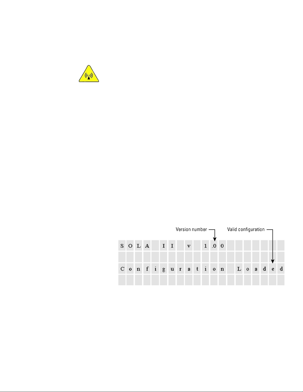
b. Verify that the display is functioning. The screen in Figure 4–1

appears, which displays the version and whether a valid configuration
is loaded.

Figure 4–1.

c. Verify that the configuration settings in the menus match the

application data sheet or system logbook.

d. Suspend the analyzer (Chapter 5) to prevent accidental injection of

sample while setting up the instrument.

4-2 SOLA II User Guide Thermo Fisher Scientific

Startup & Shutdown

Startup after

Term

Shutdown

Startup after Short-Term Shutdown

5. Apply carrier air to the instrument, and set the flows. See application data

sent with the instrument for proper settings.

a. Verify that the pyrolyzer and oven heater temperature come up to

temperature and stabilize at the control point.

b. Adjust the zero/carrier air pressure and flow again after the pyrolyzer

and oven stabilize at the correct temperature.

6. Turn on the sample flow to the instrument, and adjust it to the correct

pressure and flow. Note that this procedure varies depending on the
installed sampling system. Consult the application notes and drawings
provided with the instrument for more information.

7. Enable analysis of the sample by taking the instrument out of the suspend

mode (Chapter 5). The unit begins injecting and analyzing sample when

the instrument temperatures reach operating levels.

Short-

8. Allow the analyzer system to stabilize. Monitor the measured values on

the front panel for consistent analysis readings to determine when the
analyzer system has stabilized.

9. Calibrate the analyzer according to “Calibration” in Chapter 6. Allow

ample time for this initial calibration to stabilize. Subsequent calibrations
proceed more quickly than this initial calibration.

If starting the analyzer for the first time or if major service has been
performed, use the initial startup procedure detailed in the previous section

“Initial Startup.”

When starting the analyzer after a short-term shutdown, perform the
following:

1. Open the instrument/purge air and carrier air to the instrument. Refer to

the applications information, manuals, and drawings shipped with the
instrument, and adjust the pressure regulators to the appropriate settings.

2. Apply power to the analyzer.

Note If the X-Purge option is installed, you must follow the instructions

included in Appendix G. σ

Thermo Fisher Scientific SOLA II User Guide 4-3

Startup & Shutdown

Short-Term

Shutdown

Maintenance

Shutdown

Short-Term Shutdown

3. Allow the analyzer to warm up until the instrument stabilizes.

4. Adjust the flow rates.

5. Turn on sample to the instrument.

6. If necessary, calibrate the analyzer (“Calibration,” Chapter 6).

The analyzer includes an interlock system that prevents the injection valve
from operating until the pyrolyzer and oven temperatures reach the operating
value.

Follow this procedure when temporarily shutting down the analyzer. To shut
down the analyzer for maintenance purposes or for a long-term shutdown,
refer to the following section “Maintenance Shutdown.”

1. Turn the solenoid manifold regulator to 0 psig. Doing so blocks sample

flow to the injection valve and purges sample from the injection valve.

2. Observe reported sulfur value.

3. Do not interrupt power, instrument air, carrier or auxiliary air, or open

oven doors until reported sulfur value is less than 0.5 ppm or reported
sulfur value has not changed by more than 2% for 15 minutes.

Note Sample is purged automatically by 3-way diverter valves when power is

removed from the instrument. σ

The analyzer system must be fully shut down and the sample system
decontaminated as appropriate PRIOR to performing maintenance. Follow this
procedure when shutting down the analyzer for maintenance or a long-term
outage.

1. Close the sample flow to the instrument and purge sample from the unit

using air.

2. Turn off power to the analyzer.

4-4 SOLA II User Guide Thermo Fisher Scientific

Startup & Shutdown

Emergency

Shutdown

Emergency Shutdown

3. Allow the instrument to cool.
a. If the analyzer is used in an ATEX hazardous area with a T3 rating, do

not open the oven door for 45 minutes, 50 minutes for Zone 2 unit.

b. If the analyzer is used in an ATEX hazardous area with a T4 rating,

do not open the oven door for 140 minutes.

Caution Failure to allow adequate cooling time before opening the oven can

lead to equipment damage or injury to personnel. σ

4. Turn off all air supplies.

Caution Parts of the instrument may be hot even after power is removed.

Allow the system to cool completely before performing maintenance. σ

1. Close the sample supply to the system.

2. Turn off the main power to the system.

Thermo Fisher Scientific SOLA II User Guide 4-5

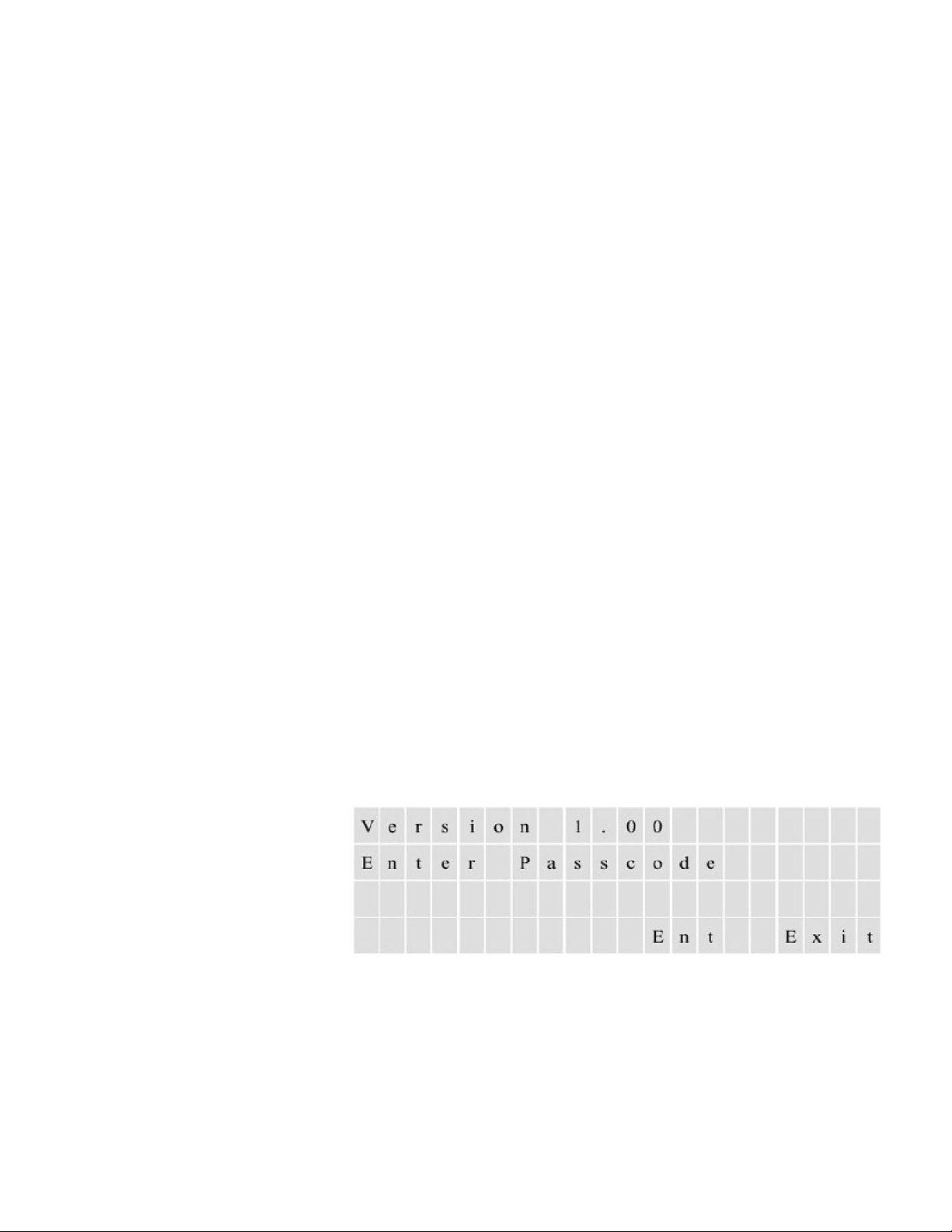
Chapter 5

The Interface

Operation

The analyzer utilizes a 4-line x 20-character, vacuum fluorescent display and 4
push buttons as the user interface. All programming and adjustments are
accomplished using the push buttons. Following is an example of how to use
the interface to enter the passcode.

1. Press any button, and you are prompted to enter the passcode, as seen in

Figure 5–1.

2. Press the button below Ent (Enter) and Figure 5–2 appears.

3. To increase the first digit’s value press the button below the up arrow

(∧). Decrease the value by pressing the button below the down arrow
(∨). When the correct number is displayed, press the button below the
right arrow (>) to enter the next digit.

4. Repeat the process used to enter the first digit for the remaining digits.

5. When you have completed this, press the button below Done.

You can access all program features and edit parameters by following these
steps.

Figure 5–1.

Thermo Fisher Scientific SOLA II User Guide 5-1

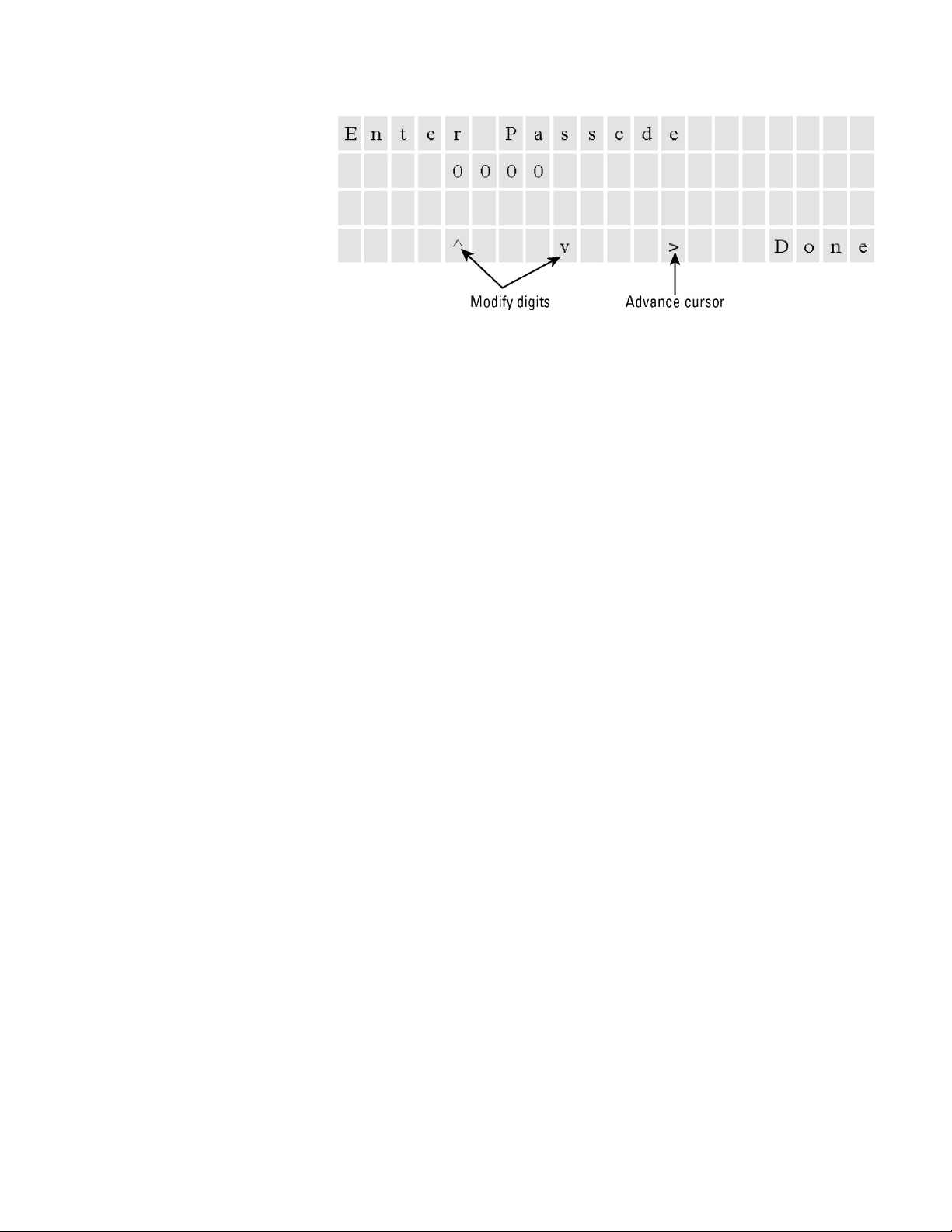
Operation

Suspended to suspend the analysis. In suspended mode, the

Active

Begin Analyzing

Suspending an

Analysis

Begin Analyzing

Figure 5–2.

1. If the analyzer is shut down, start up the instrument by following the

appropriate set of instructions in Chapter 4.

2. If the system power is off, open the instrument and carrier air flows to

the analyzer, and adjust the pressures to the appropriate settings (refer to
application data that shipped with the analyzer).

3. Open sample flow to the analyzer.

4. Apply power to the instrument.

5. Analysis begins automatically when the pyrolyzer reaches operating

temperature. If you need to change the configuration, press any button,
and enter the passcode.

Follow these steps to suspend an analysis.

1. Enter the Analyzer Mode top-level menu (Figure 5–3).

2. Select

3. To resume the analysis, go to the Analyzer Mode menu, and select

analyzer stops injecting, and the sample diverter valve allows only air to
run through the burner and mixing chamber.

.

5-2 SOLA II User Guide Thermo Fisher Scientific

Operation

Injection Valve

Failure Alarm

Injection Valve Failure Alarm

Figure 5–3.

Over time, the injection valve begins to wear, resulting in an increased
potential for port-to-port leakage of sample. Such leakage can cause erroneous
measurement and materials buildup in the system. When the analyzer detects
sample leakage through the injection valve, it triggers the Injection Valve
Failure alarm and switches the sample diverter valves to flow air through the
injection valve rather than sample.

Note The Injection Valve Failure alarm must be acknowledged after valve

repair or replacement. σ

If an injection valve begins leaking due to damage or wear, excess sample
begins flowing to the pyrolyzer. This extra load of sample in the pyrolyzer
exceeds the ability to fully combust the materials in the sample. When these
incompletely combusted materials enter the PUVF optical bench, they absorb
UV light.

The PUVF includes a system to monitor and compensate for decreases in the
UV light output as the bulb ages. However, in the case of injection valve
failure, the PUVF system begins rapidly increasing the UV lamp output in an
effort to compensate for the absorption of UV by incompletely combusted
sample products. The user can enter the rate of change that triggers this
alarm. The programmable range is from 1 to 50 V/30 seconds. If the analyzer
detects the programmed rate of change in UV lamp voltage, it triggers the
Injection Valve Failure alarm to protect the system and reduce the
stabilization time for the PUVF bench on system restart.

When the Injection Valve Failure or Chamber Flow alarm activates, a pair of
sample diverter valves switches to flow air through the injection valve instead
of sample. This prevents excess sample and incomplete combustion products
from further contaminating the system. The diverter valves switch air to the
injection valves under the following conditions:

λ Injection Failure alarm

λ Instrument power loss

λ Instrument air loss

λ Analysis suspension

Thermo Fisher Scientific SOLA II User Guide 5-3

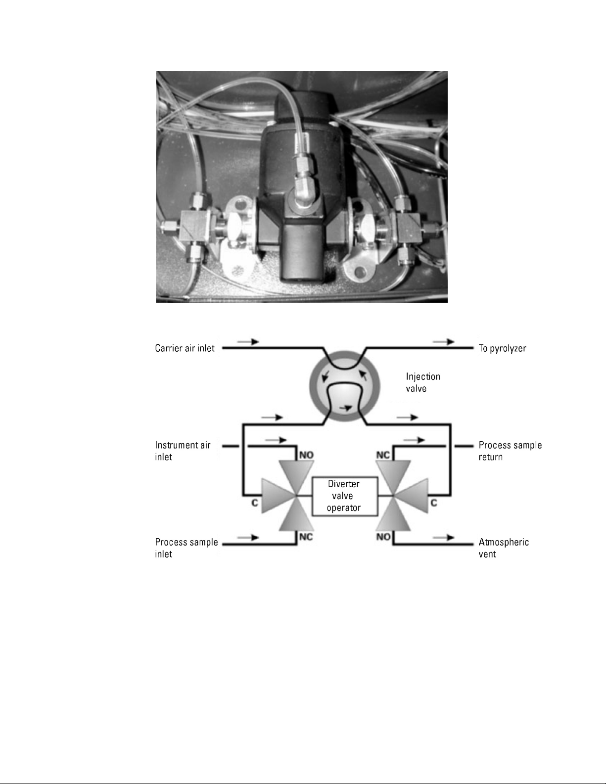
Operation

Injection Valve Failure Alarm

Figure 5–4. Sample diverter valves

Figure 5–5. Sample diverter valves functional diagram

5-4 SOLA II User Guide Thermo Fisher Scientific

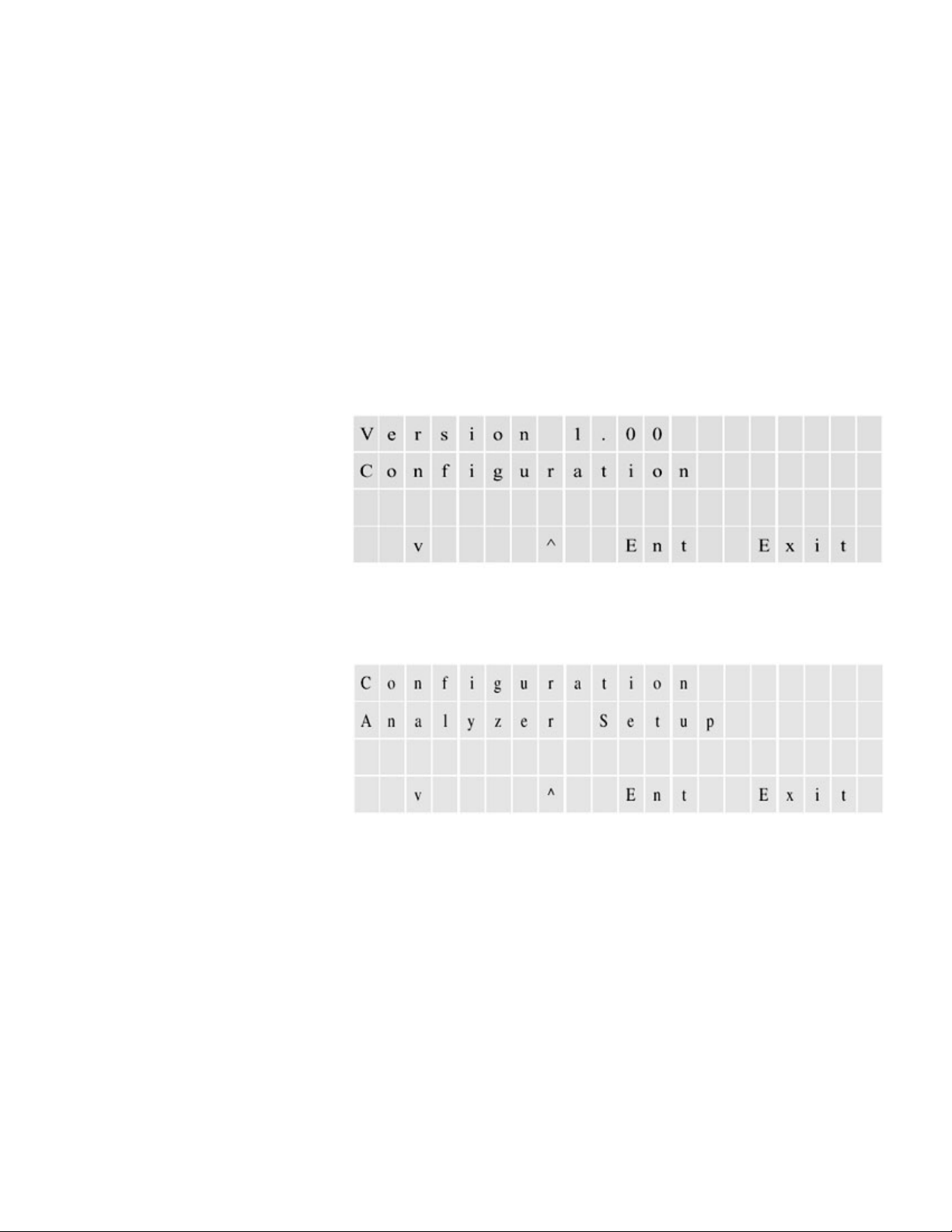
Chapter 6

Enter

Analyzer Setup

Configuration

There are five top-level menus; this chapter addresses the Configuration menu
(Figure 6–1). The Configuration menu contains 10 setup menus: Analyzer
Setup, Stream Setup, Clock Setup, Modbus Setup, Dual Range Setup, Inject
Setup, Autocal Setup, Alarms Setup, Calibration Setup, and Density
Compensation Setup.

Figure 6–1. Top-level configuration menu

1. Access the submenus within the Analyzer Setup menu by pressing

Figure 6–2.

.

2. The first submenu is Program Passcode. The factory default is 0000. If the

passcode remains 0000, you are not required to enter the passcode to

Thermo Fisher Scientific SOLA II User Guide 6-1

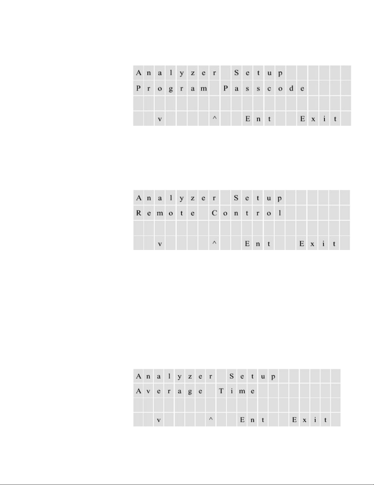
Configuration

Analyzer Setup

access the menus. Change the passcode to prevent unauthorized access to
the menus.

Figure 6–3.

3. Return to the Analyzer Setup menu. Press the down arrow until the

Remote Control submenu appears (Figure 6–4), allowing you to
enable/disable the remote control function. “DCS & External Connections”
in Chapter 3 addresses which functions may be operated remotely.

Figure 6–4.

4. The Average Time submenu allows you to set the averaging time. The

average time is a period (1–240 seconds) during which the analyzer takes
SO2 measurements used to determine a moving average of the results. For
example, if you set the averaging time to 10 seconds, the average
concentration of the last 10 seconds is output at each update. If you set
the averaging time to 60 seconds, the average concentration of the last 60
seconds is output at each update. Thus, lower averaging time means faster
response to concentration changes. Longer averaging times are typically
used to smooth output data.

See the figure below.

Figure 6–5.

6-2 SOLA II User Guide Thermo Fisher Scientific

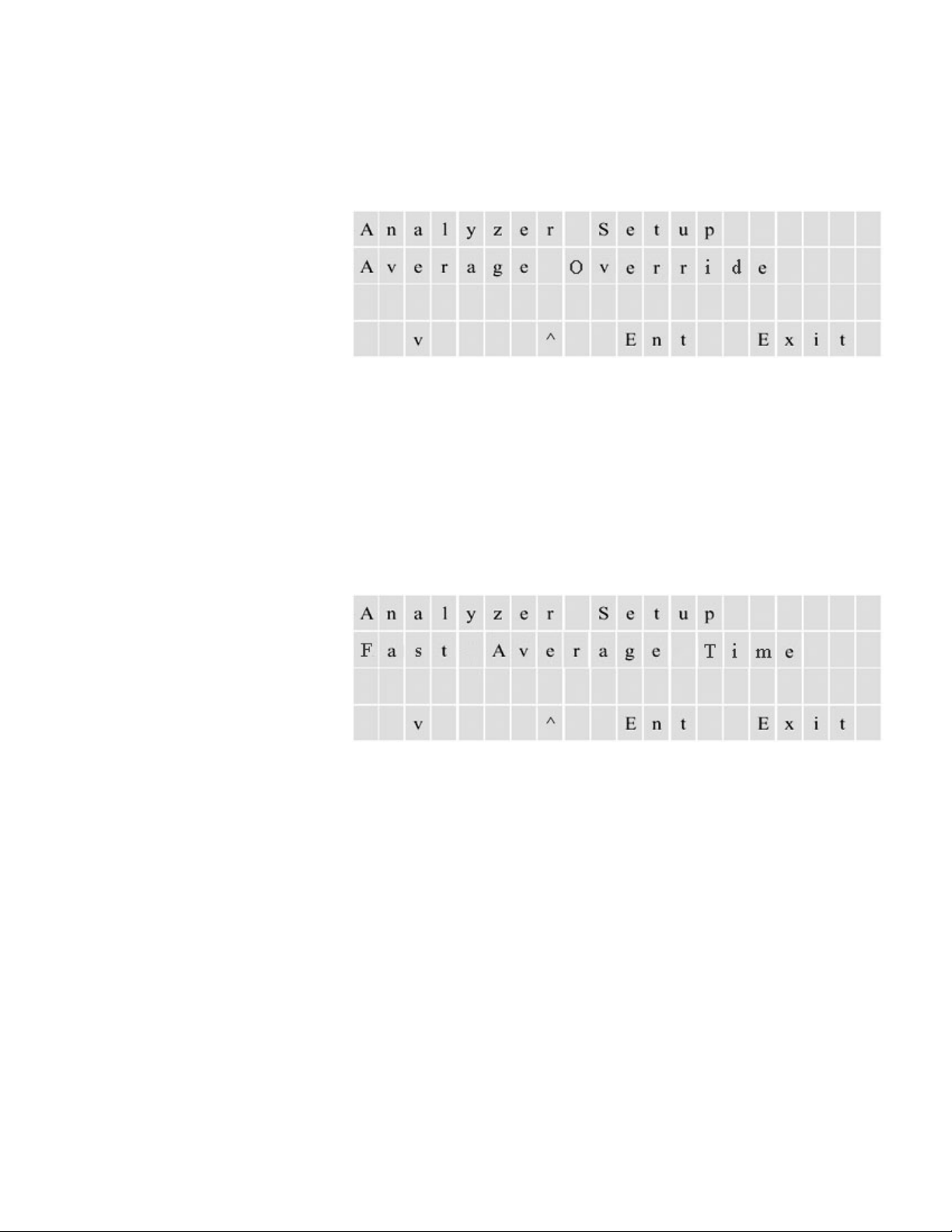
Configuration

Analyzer Setup

5. The average override is expressed as a percentage of change and

determines when the unit switches to the fast average. As the reading
stabilizes at the new level, the analyzer progressively increases the average
used until it reaches the programmed average time.

Figure 6–6.

6. The fast average time provides the ability to respond to changes faster

without sacrificing stability achieved using a longer average time.

Note Both the regular and fast average times need to be set at multiples of

the injection rate. For example, if the rate is two injections per minute,
averages should be set to 30, 60, 90, 120, 150, 180, 210, or 240 seconds. σ

Figure 6–7.

7. There are three selections within this submenu: NONE, 4 to 20 mA, and

Flow Switch.

Thermo Fisher Scientific SOLA II User Guide 6-3

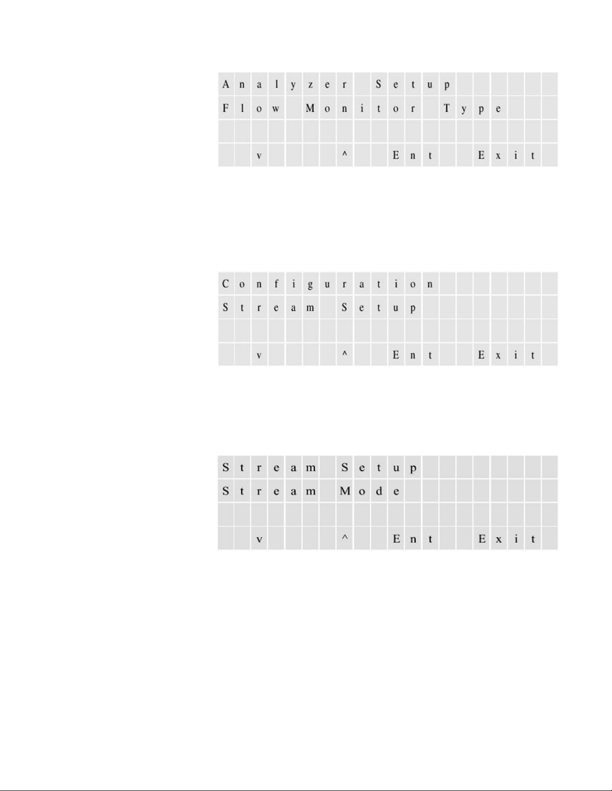
Configuration

Enter

Stream Setup

Stream Setup

Figure 6–8.

This section steps through the menu items in the Stream Setup menu.

1. Access the submenus within the Stream Setup menu by pressing

Figure 6–9.

2. The Stream Mode submenu allows you to configure the analyzer to

continuously monitor stream 1 (Stream 1), continuously monitor stream 2
(Stream 2), or to alternate between the streams (Timed Stream).

.

Figure 6–10.

3. If you select the Timed Stream option as the mode, you must determine

the dwell time. Dwell time is the period of time the analyzer monitors one
stream before it begins monitoring the other. Figure 6–11 displays the

6-4 SOLA II User Guide Thermo Fisher Scientific

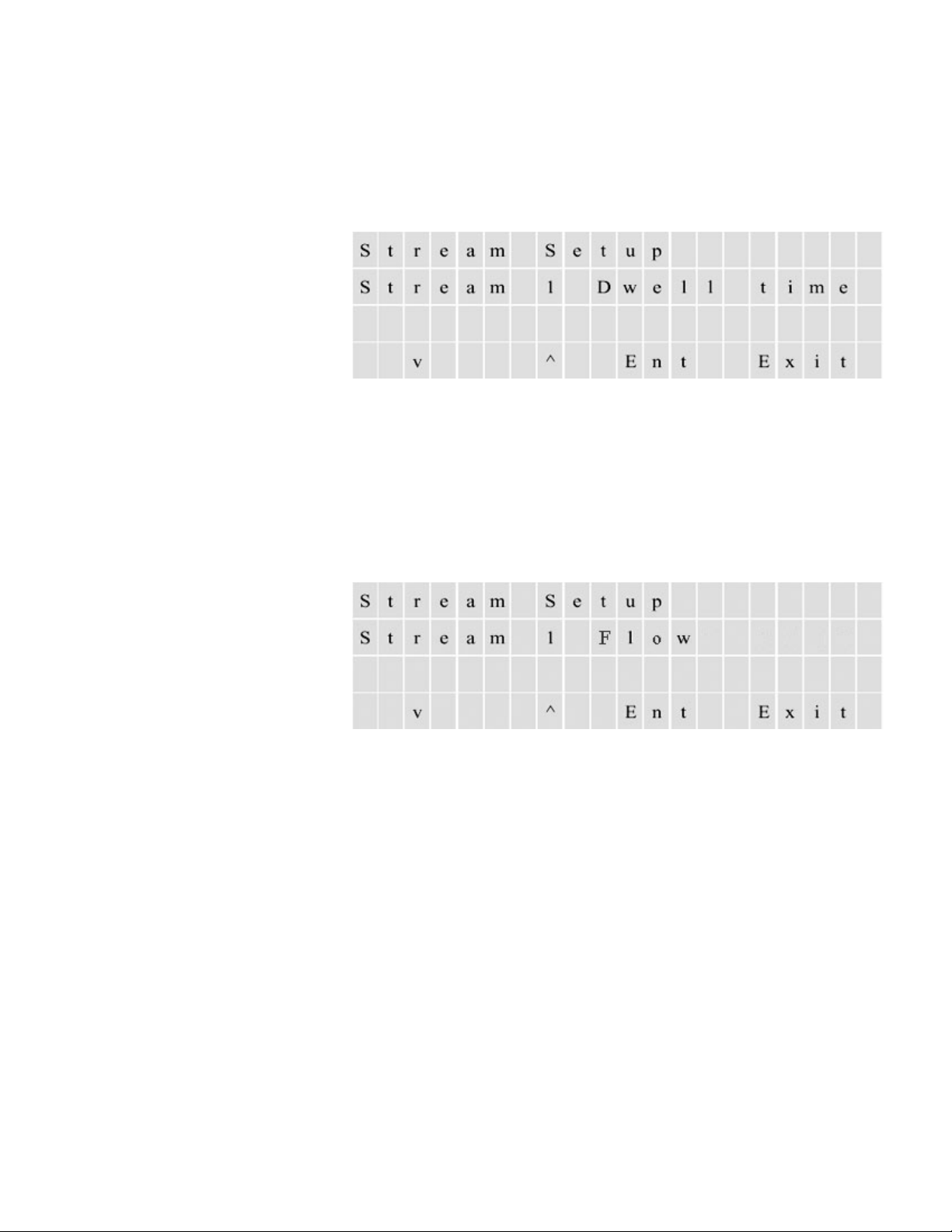
Configuration

Stream Setup

submenu that allows you to program the dwell time for stream 1 (the
length of time the analyzer stays on stream 1 before it begins monitoring
stream 2). You can then program the dwell time for stream 2 (the length
of time the analyzer stays on stream 2 before returning to stream 1).
Dwell time may be from 1 to 1440 minutes (24 hours).

Figure 6–11.

4. When using the second stream for validation or during the calibration

cycles, it might be desirable to reduce the flow in order to conserve
calibration/validation standards. You can program each stream for high or
low flows. If equipped with the second stream option, the analyzer has
NO and NC pneumatic outputs to control the flow in the sampling
system. The calibration and validation routines always select the low flow.

Figure 6–12.

5. If you select the Timed Stream option, you must also determine how long

the analyzer purges the line before it begins analyzing the other stream.
This period is called the purge time. In respect to calibration, purge time
is how long the analyzer purges the line before it begins analyzing the
calibration stream. You can set the purge time between 1 and 9999
seconds.

See the figure below.

Thermo Fisher Scientific SOLA II User Guide 6-5

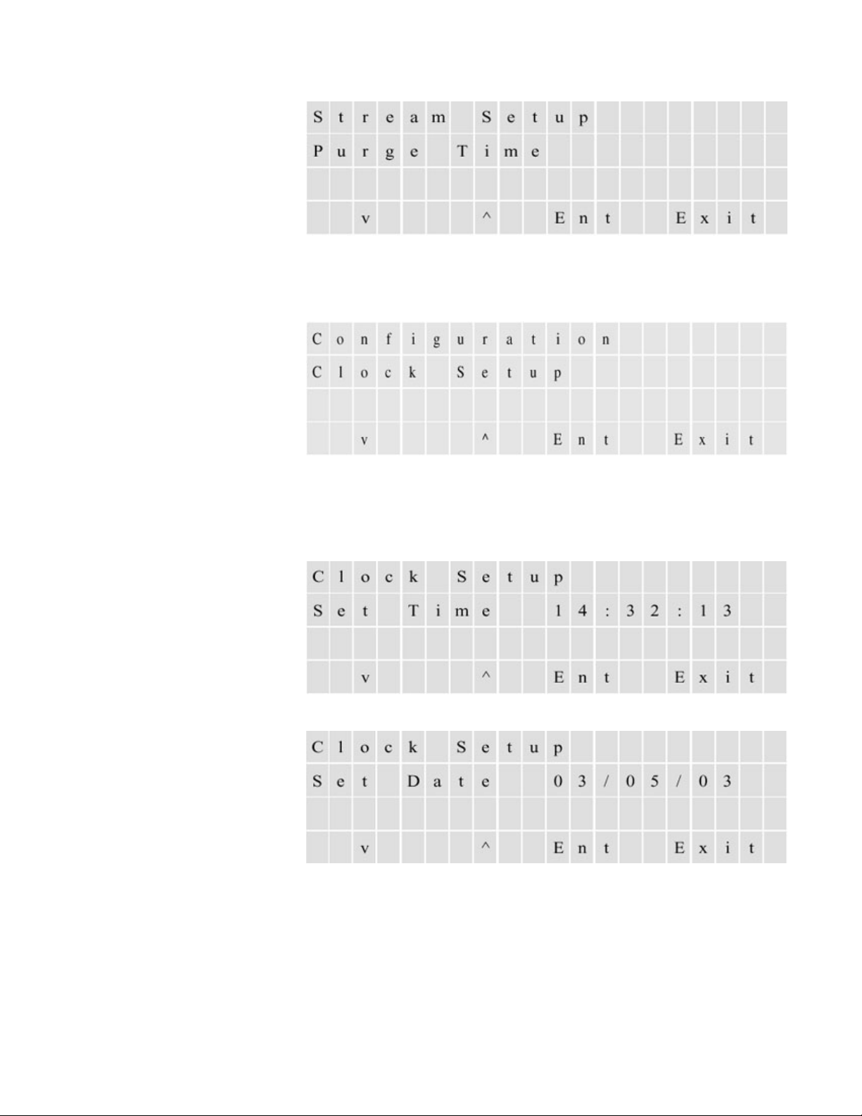
Configuration

Clock Setup

Clock Setup

Figure 6–13.

1. Access the Clock Setup menu to change the time and date.

Figure 6–14.

2. Enter the time in hh:mm:ss, 24-hour format and the date (in the following

screen) in mm/dd/yyyy format.

Figure 6–15.

Figure 6–16.

6-6 SOLA II User Guide Thermo Fisher Scientific

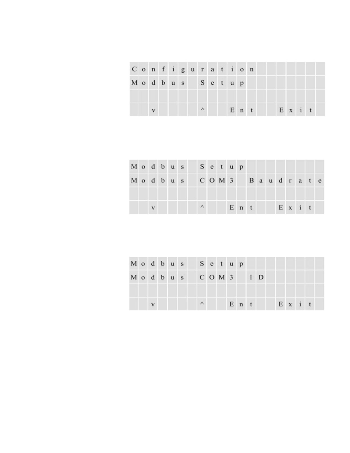
Configuration

Disable

Modbus Setup

Modbus Setup

1. The Modbus Setup menu enables to you set the baud rates and IDs for

COM 3 and COM 4.

Figure 6–17.

2. Select one of the baud rates available for RS485 Com 3 (38400, 19200,

9600, 4800, 2400, and 1200 bps), or select

.

Figure 6–18.

3. Set the ID (network address) for Com 3. The address can be between 1

and 255.

Figure 6–19.

Set the baud rate and the ID for COM 4 in the same manner using the
submenus for COM 4.

Thermo Fisher Scientific SOLA II User Guide 6-7

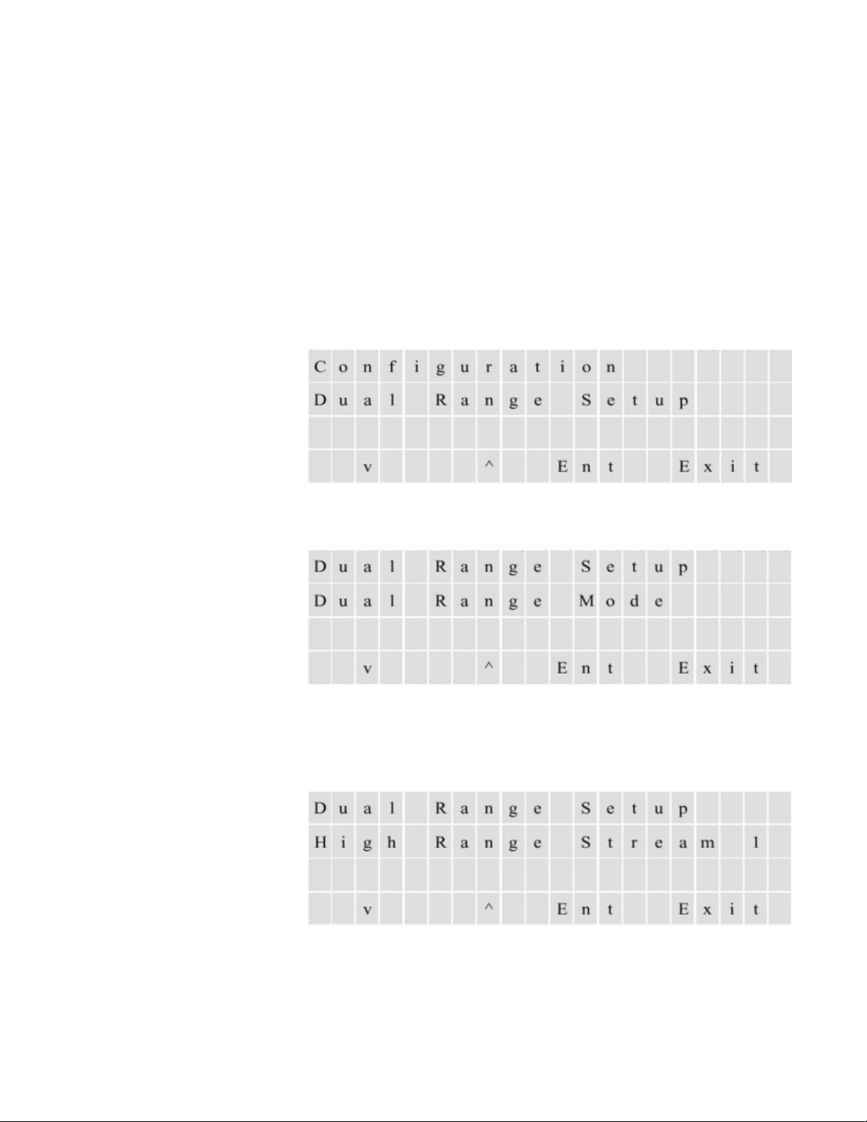
Configuration

Dual Range

Setup

Dual Range Setup

This menu allows you to set the dual range mode.

1. Set the dual range mode to Remote Range Select or to Auto Range for the

4–20 mA output signal. If you select Auto Range, the 4–20 mA output
signal switches to high range when the reading goes above the low range
full scale value. When the signal drops below 90% of the low range full
scale value, the system switches back to low range.

When Remote Range Select is enabled, output scaling is controlled by a
remote contact input. When the input contacts are open, the system
operates on low range. When the input contacts are closed, the system
operates on high range.

Figure 6–20.

Figure 6–21.

2. The submenu shown below enables you to specify the full scale value (20

mA) for the high range of stream 1 as output on the 4–20 mA signal.

Figure 6–22.

6-8 SOLA II User Guide Thermo Fisher Scientific

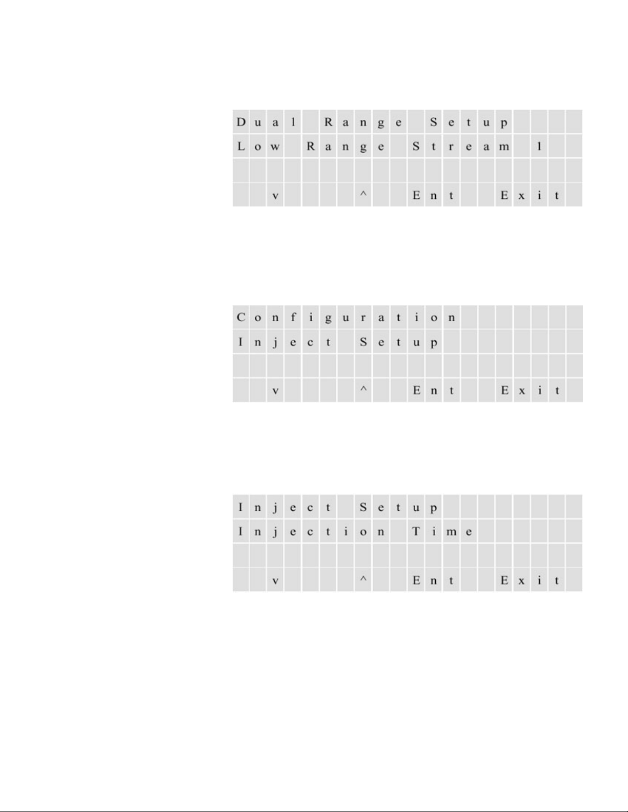
Configuration

Inject Setup

Inject Setup

3. The submenu shown below enables you to specify the full scale value (20

mA) for the low range of stream 1 as output on the 4–20 mA signal.

Figure 6–23.

Set the 20 mA scaling for the high and low ranges for stream 2 using the
submenus for stream 2.

1. Enter the Inject Setup menu to set injection parameters.

Figure 6–24.

2. The injection time is the amount of time that the injection valve stays in

the injection position. Set the inject time at half of the inject rate (1 to
9999 seconds).

Figure 6–25.

Thermo Fisher Scientific SOLA II User Guide 6-9

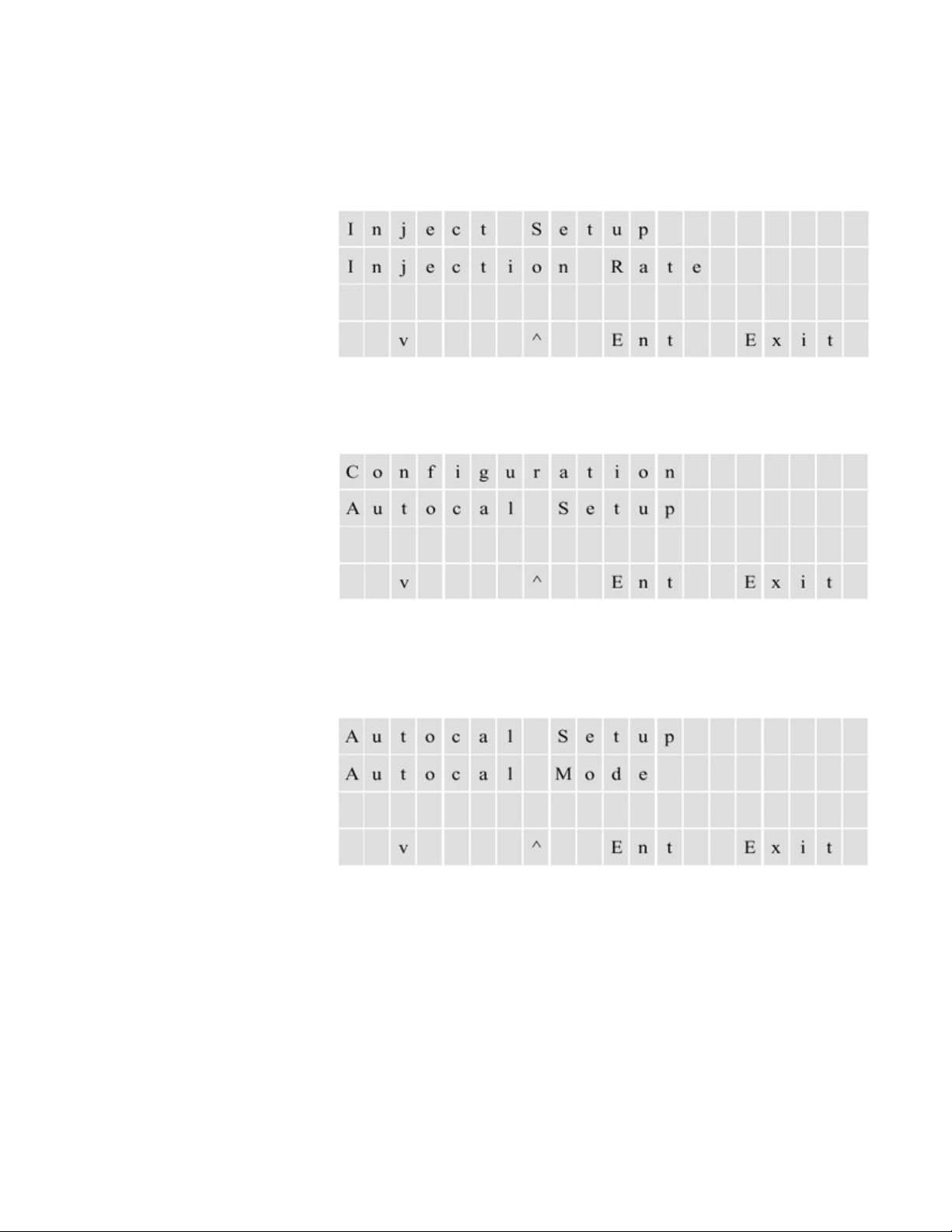
Configuration

if a 6-port valve is

used, set the rate to twice the desired injection interval.

Autocal Setup

Autocal Setup

3. Set the injection rate (the amount of time to wait between sample

injections). The rate can be between 2 and 9999 seconds. A 6-port valve
injects at each actuator move in both positions. Thus,

Figure 6–26.

1. Enter this menu to configure the autocal function.

Figure 6–27.

2. The Autocal Mode submenu allows you to enable/disable periodic

automatic calibration of the analyzer.

Figure 6–28.

6-10 SOLA II User Guide Thermo Fisher Scientific

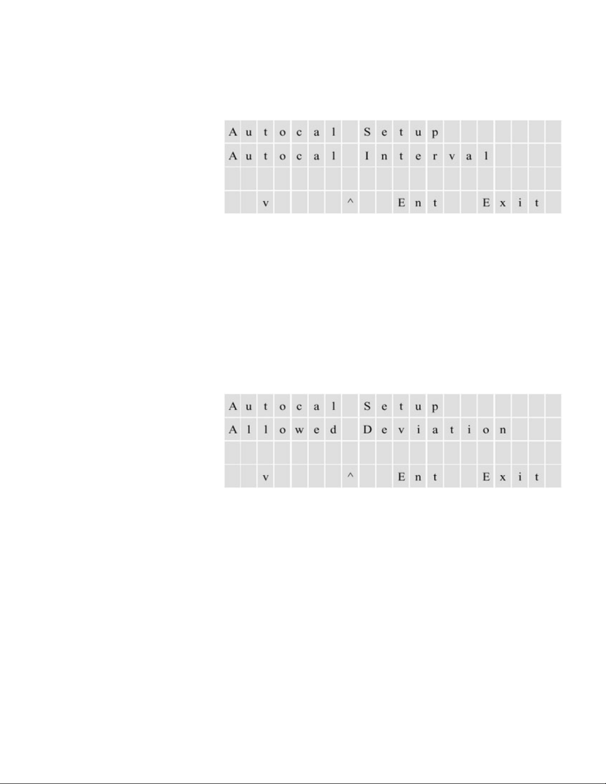
Configuration

Autocal Setup

3. If the autocal function is enabled, access the Autocal Interval submenu to

specify the length of time between automatic calibrations. The interval can
be set between 1 to 9999 minutes.

Figure 6–29.

4. Allowed Deviation is the percentage of deviation from the programmed

autocal value that is acceptable without updating the calibration factor.
This function is used primarily when using calibration sample for system
validation tests. When an automatic calibration is performed, the analyzer
calculates the percentage the new calibration factor deviates from the
previous calibration factor. If the percentage deviation is less than the
allowed deviation, the system keeps the previous calibration factor. If the
deviation exceeds the allowed deviation and is less than the Recal
Deviation, the new calibration factor replaces the previous one.

Figure 6–30.

5. Recal Deviation is the percentage of deviation from the programmed

autocal value that is acceptable to compute new calibration factors. Access
this submenu to specify this percentage. Note that an Autocal Fail alarm
activates if the deviation exceeds the amount specified.

See the figure below.

Thermo Fisher Scientific SOLA II User Guide 6-11

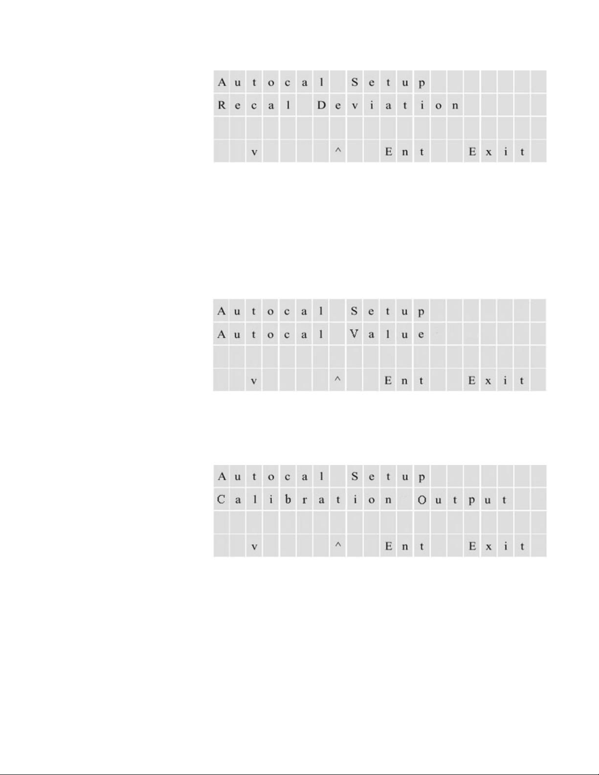
Configuration

Autocal Setup

Figure 6–31.

6. If set to recalibrate, the calibration line moves, maintaining the same

slope. It is similar to the manually initiated adjust reading function.
Setting both deviations to the same value disables the autocal, making it a
validation only function.

The autocal/validation functions can be used with a programmable value
other than the high calibration value.

Figure 6–32.

7. You can direct the reading during auto calibration to stream 1 or 2, 4–20

mA output, or none of the outputs.

Figure 6–33.

6-12 SOLA II User Guide Thermo Fisher Scientific

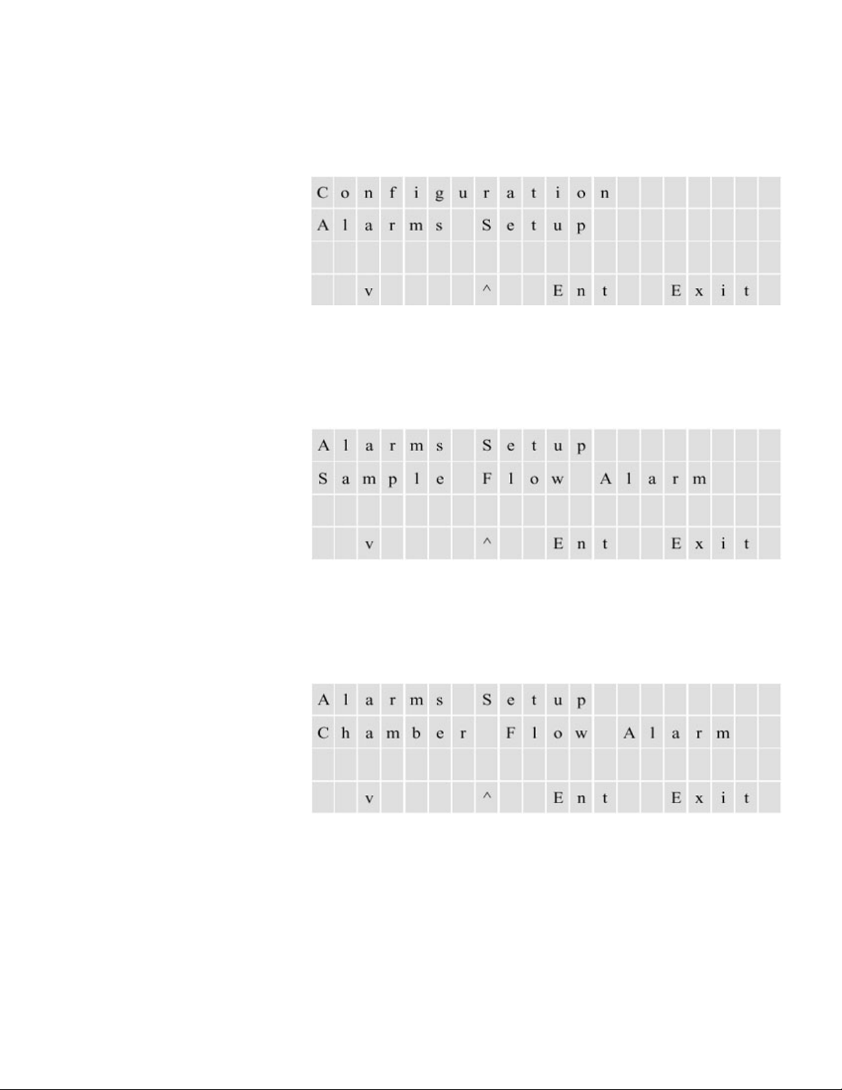
Review the following for instructions pertaining to alarm setup.

Enter

Alarms Setup

Configuration

Alarms Setup

1. Access the menu items by pressing

.

Figure 6–34.

2. The Sample Flow alarm is available if the flow meter option is present.

The set point for the low sample flow alarm is a percentage of the 4–20
mA signal from the flow meter.

Figure 6–35.

3. To set up a Chamber Flow alarm, enter the set point at which the low

flow alarm for the flow measured at the detector chamber in the PUVF
should activate. The value can be from 0 to 1000 cc/m.

Figure 6–36.

Thermo Fisher Scientific SOLA II User Guide 6-13

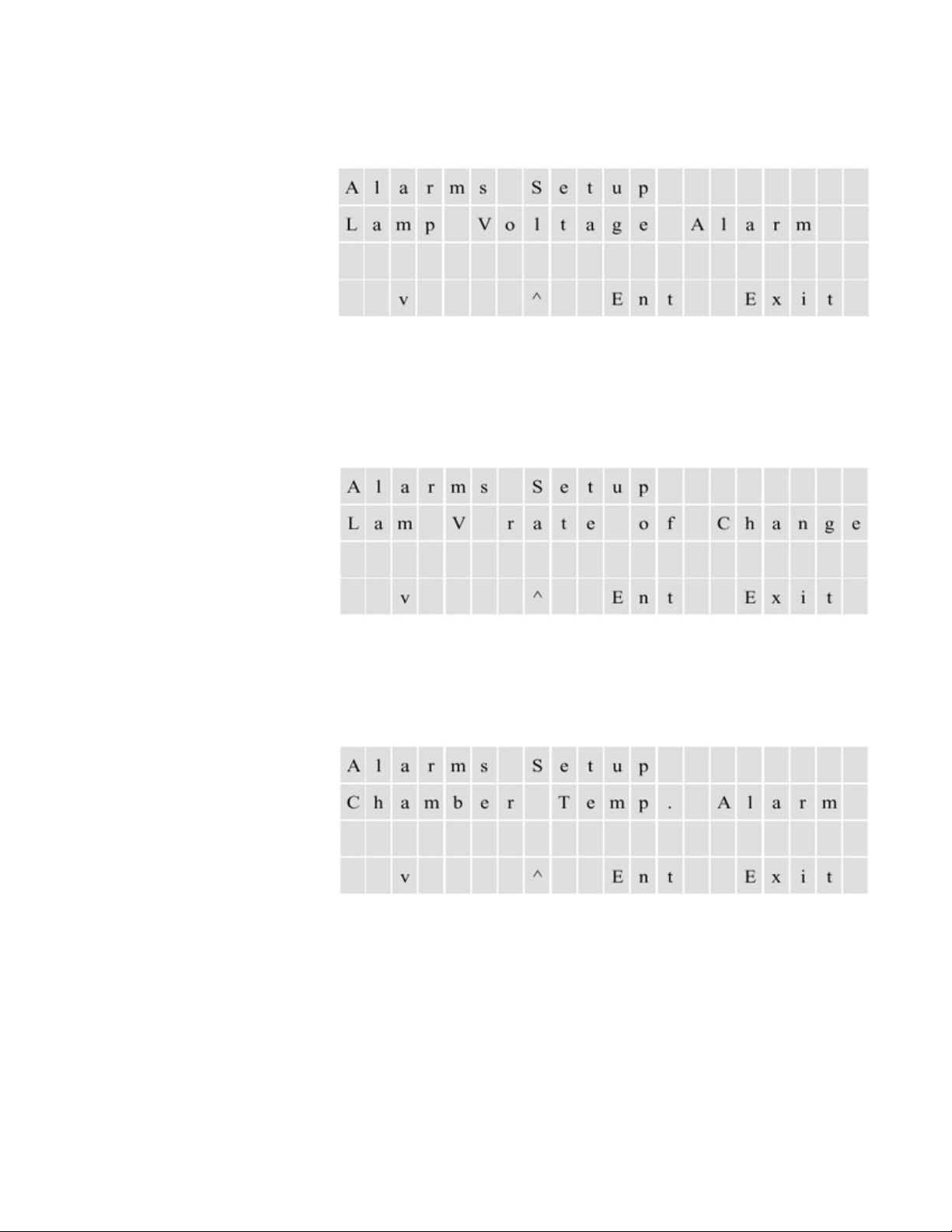
Configuration

Alarms Setup

4. To set up a Lamp Voltage alarm, enter the maximum lamp voltage at

which the alarm should activate. The value can be from 0 to 1200 V.

Figure 6–37.

5. Set up a Lamp Voltage Rate of Change alarm by entering the rate of

change in lamp voltage at which the alarm should activate. The value can
be from 1 to 50 V per 30 seconds.

Figure 6–38.

6. Set up a Chamber Temperature alarm by entering the +/- deviation from

45°C at which the alarm should activate.

Figure 6–39.

6-14 SOLA II User Guide Thermo Fisher Scientific

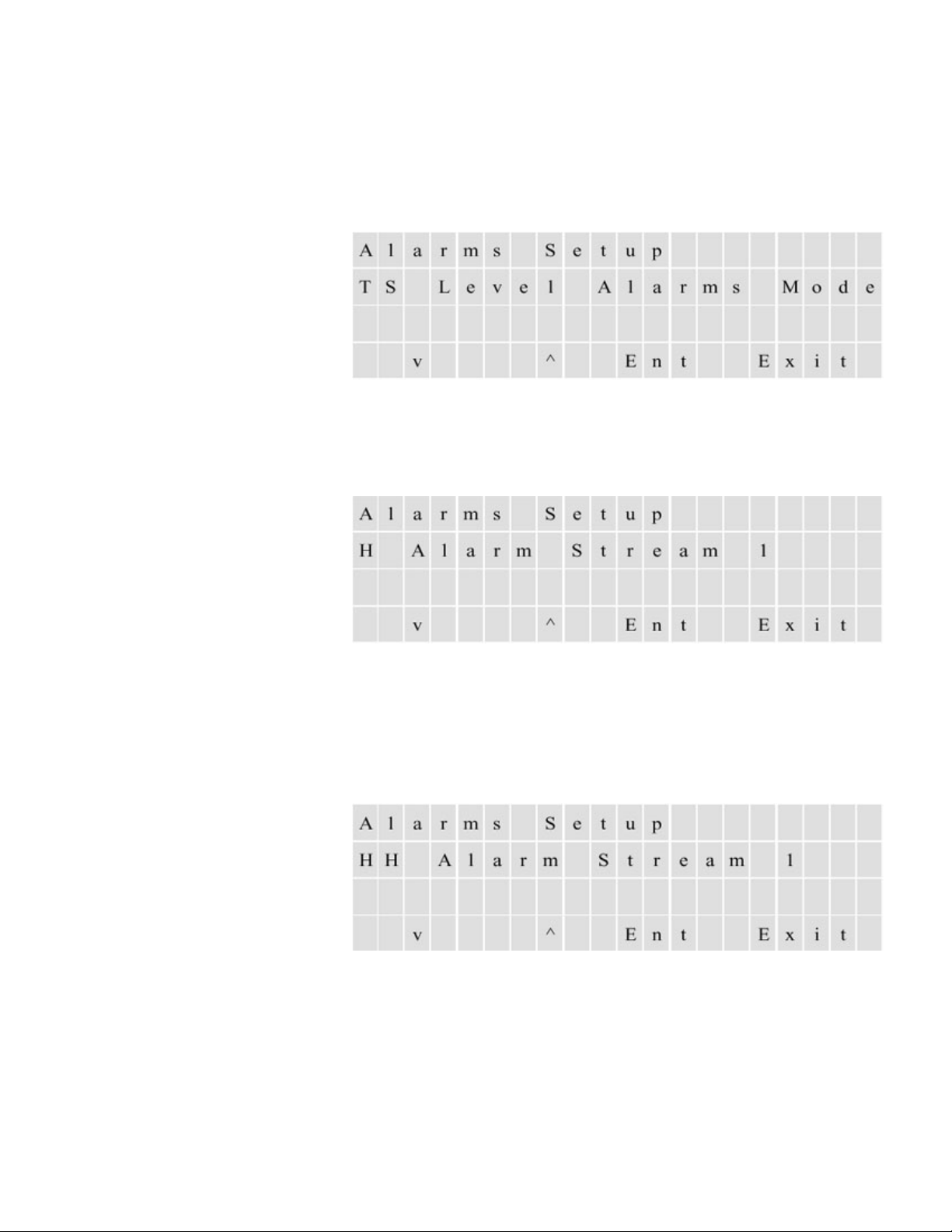
Configuration

Alarms Setup

7. Select one of the TS Level Alarms modes. Select Disable, Non Latching, or

Latching mode for the concentration alarms. If you select nonlatching, the
alarm clears when the measured concentration drops below the associated
value. If you select latching, the alarm must be acknowledged before it will
clear.

Figure 6–40.

8. Set the High Alarm for stream 1 by entering the first level of high

concentration for stream 1 at which the alarm should activate.

Figure 6–41.

9. Set the High High alarm for stream 1 by entering the second level of high

concentration for stream 1 at which the alarm should activate. There are
also submenus for setting the high alarm and the high high alarm for
stream 2. If applicable, set these alarms as done for stream 1.

Figure 6–42.

Thermo Fisher Scientific SOLA II User Guide 6-15

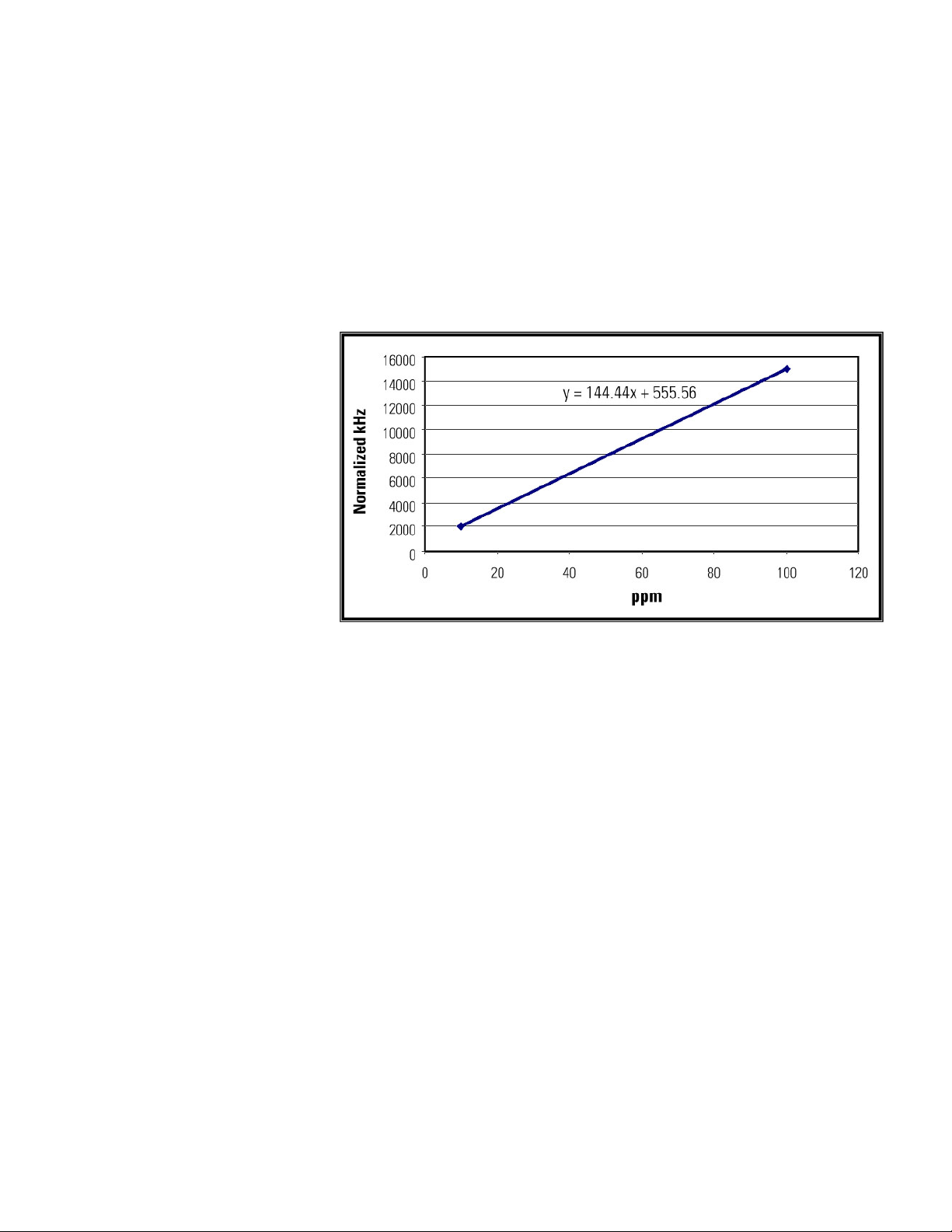
Configuration

Calibration Setup

Calibration

Overview

Calibration

The analyzer requires a two-point linear calibration. During the calibration
procedure the average of the raw detector signals corresponding to two
known sulfur concentrations are latched by the unit and retained in non­volatile memory.

During normal operation, the average detector reading is interpolated on the
line to derive the sulfur concentration reported.

The graph below illustrates a SOLA II calibration.

Figure 6–43.

Prior to calibrating the instrument, the sulfur concentration expected at the
two points must be entered in the calibration setup menus (Configuration >

low calibration values.

For the graph above, the values would be:

Low cal value = 10.00 ppm Low cal = 555.600 kHz

High cal value = 100.00 ppm High cal = 15000.000 kHz

The high calibration value needs to be as close as possible to the full range
sulfur concentration expected in the process, and the low calibration value is
normally set to zero so that only one standard is required for calibration.

). In the software, these points are referred to as high and

6-16 SOLA II User Guide Thermo Fisher Scientific

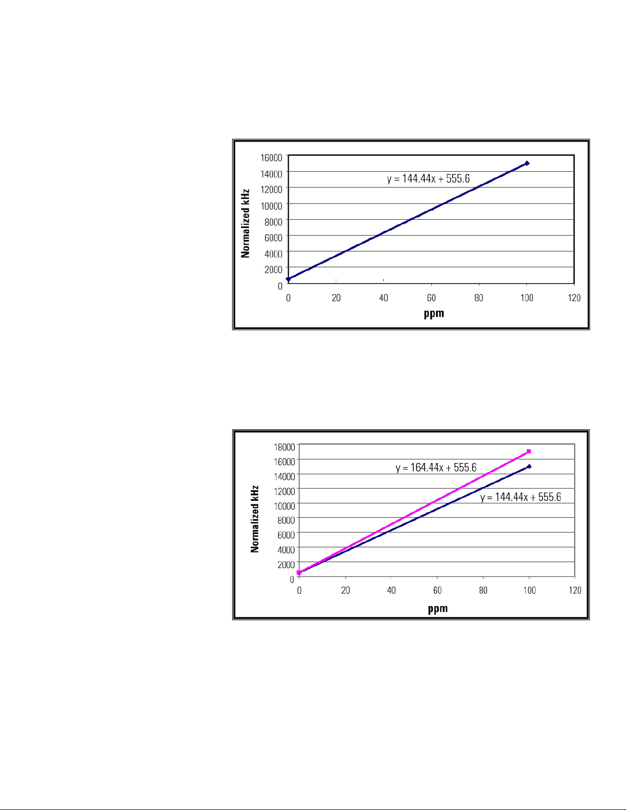
The values and a graph for a typical calibration are shown below.

Low cal value = 0.00 ppm Low cal = 555.600 kHz

High cal value = 100.00 ppm High cal = 15000.000 kHz

Figure 6–44. Typical SOLA II calibration

Configuration

Calibration

The high and low calibration can be performed independently. Changing
either one of the calibration points will change the slope of the line. This is
illustrated in the next two graphs.

Figure 6–45. High calibration

Thermo Fisher Scientific SOLA II User Guide 6-17

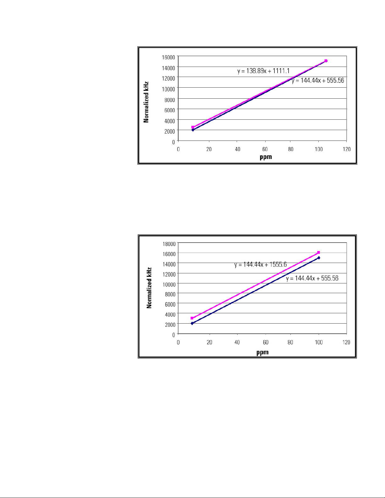
Configuration

Calibration

Figure 6–46. Low calibration

If necessary, the Adjust Reading function in the Calibration Setup menu can
be used to correct the calibration by moving the line without changing the
slope (see Figure 6–47). Enabling the Autocal function will cause the software
to perform this correction automatically.

Figure 6–47. Corrected calibration

Several calibration functions can be performed. These are discussed in the
following sections.

6-18 SOLA II User Guide Thermo Fisher Scientific

Configuration

Low Cal Value

Recalibrate Low

YES

Performing a Low

Calibration at Zero*

Calibration

*No injections

Note This is the most common form of low calibration that requires only one

standard. For SOLA II Trace, it is recommended that a low concentration
standard be used. σ

Note To prevent repetition, these sections do not include screen shots. Each

menu item within the Calibration Setup menu is shown in “Calibration Setup

Menu Items.” σ

To perform a low calibration with no injections, follow the steps below.

1. Go to Configuration > Calibration Setup >

. Set the low

calibration value to zero.

2. Exit the Calibration Setup menu.

3. Reduce the pressure at the solenoid manifold air regulator to zero (this is

the bottom regulator located in the pneumatic cabinet). Lowering the
solenoid manifold pressure will accomplish two things:

a. The diverter valve will switch to the diverter position blocking the

sample.

b. The injection valve will stop injecting, letting only the carrier gas run

through the system.

4. Let the unit run until the sulfur concentration reported is stable.

5. Go to Configuration > Calibration Setup >

. Press

to

accept the new low calibration.

At this point, the average of the detector signal is latched to correspond to a
zero sulfur concentration.

Thermo Fisher Scientific SOLA II User Guide 6-19

Configuration

High Cal Value

Purge Time

Enter

Performing a High

Calibration

The Calibrate High

Function

The Recalibrate High

Function

Calibration

Performing a high calibration can be achieved in two ways, depending on the
sample conditioning system installed.

The high calibration standard is normally contained in a pressurized cylinder.
The pneumatic output of the analyzer can be used to switch the
corresponding selection valve in the SCS, or the high calibration standard can
be manually introduced to the analyzer. Based on this, the Calibration Setup
menu offers two functions:

λ Calibrate High: Used when the analyzer is expected to switch the valves.

λ Recalibrate High: Used when the calibration standard is introduced

manually to the analyzer.

1. Go to Configuration > Calibration Setup >

. Set the high

calibration value to match the concentration of the standard used.

2. Step down to the Average Cal Readings screen. It is recommended that

you set this value to the maximum (240).

3. Exit the Calibration Setup menu, and go to Configuration > Stream Setup

>

. Set this value. It should be long enough for the unit to
stabilize (time varies depending on the location of the switching valve in
the SCS and the flow rate of the sample). Exit this menu.

4. Go back to the Calibration Setup menu. Step down to the Calibrate High

screen, and press

to perform the calibration.

At this point, the analyzer will energize the calibration solenoid and start a
purge cycle. Once the purge cycle is completed, the detector reading will be
averaged for the programmed number of calibration readings (readings are
performed once a second). The resulting average will be latched to correspond
to the high calibration value concentration.

6-20 SOLA II User Guide Thermo Fisher Scientific

Configuration

Cal Inlet

High Cal Value

Recalibrate High

YES

Adjust Reading

Adjusting the

Reading

Calibration

Use this function if manually introducing the high calibration standard to the
analyzer.

Note It is possible to force the calibration solenoid to turn on by going to

Configuration > Stream Setup >

and selecting ON. If you do this, you
can use the Recalibrate High function on systems where the analyzer
pneumatic output selects the calibration stream. σ

Note It is important to remember that if the calibration standard is

introduced manually and running as stream one, density compensation must
be turned off if used. σ

1. Go to Configuration > Calibration Setup >

. Set the high
calibration value to match the concentration of the standard used. Exit the
menu.

2. Connect the calibration standard to the unit, and let it flow through the

injection valve.

3. Let the reported concentration reach a new value and stabilize.

4. Go to Configuration > Calibration Setup >

. Press

to

accept the new high calibration.

At this point, the current average of the detector signal is latched to
correspond to the high calibration value concentration.

If the reported value of the SOLA II does not match a known sample value or
the standard flowing through the instrument, you can adjust the reading. To
do so, go to Configuration > Calibration Setup >

. The current
reading will be displayed in an editing screen so that you can modify the
reading to match the desired reading.

Note Do not use this function if the difference between the expected reading

and the analyzer’s reported reading is significant. The Adjust Reading function
should only be used for making minor corrections to the calibration. Using
this function improperly can momentarily hide malfunctions in the unit that
need to be corrected. σ

Thermo Fisher Scientific SOLA II User Guide 6-21

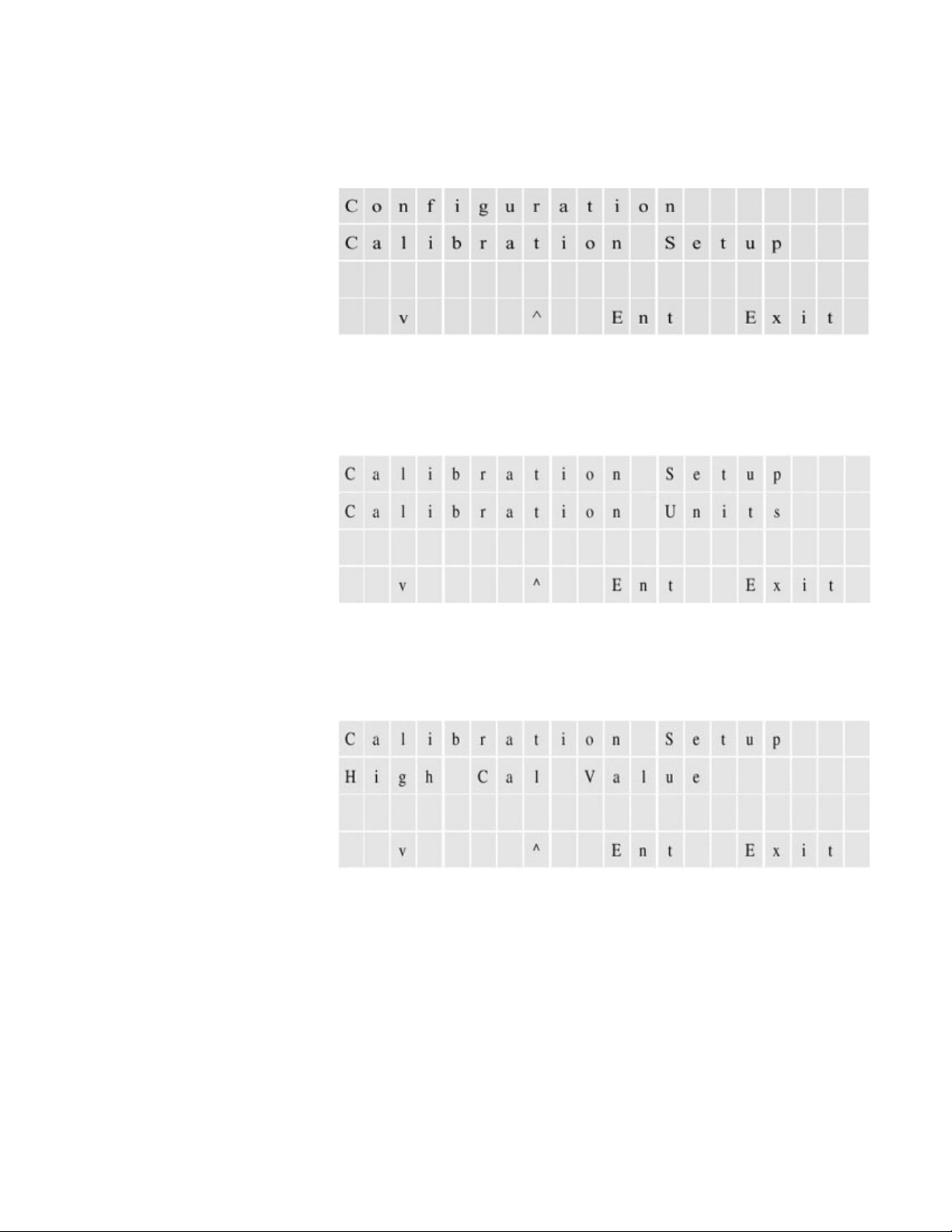
Configuration

Calibration Setup

Menu Items

Calibration

This section contains the menu items within the Calibration Setup menu in
the order they appear. Specific instructions on the various calibration
functions are discussed in the previous sections.

Figure 6–48. Main menu heading

1. Select the engineering unit related to the concentration entered for the

calibration values: ppm, ppb, or mg/L.

Figure 6–49.

2. Enter the concentrations of the high calibration standard. See “Performing

a High Calibration” for more.

Figure 6–50.

6-22 SOLA II User Guide Thermo Fisher Scientific

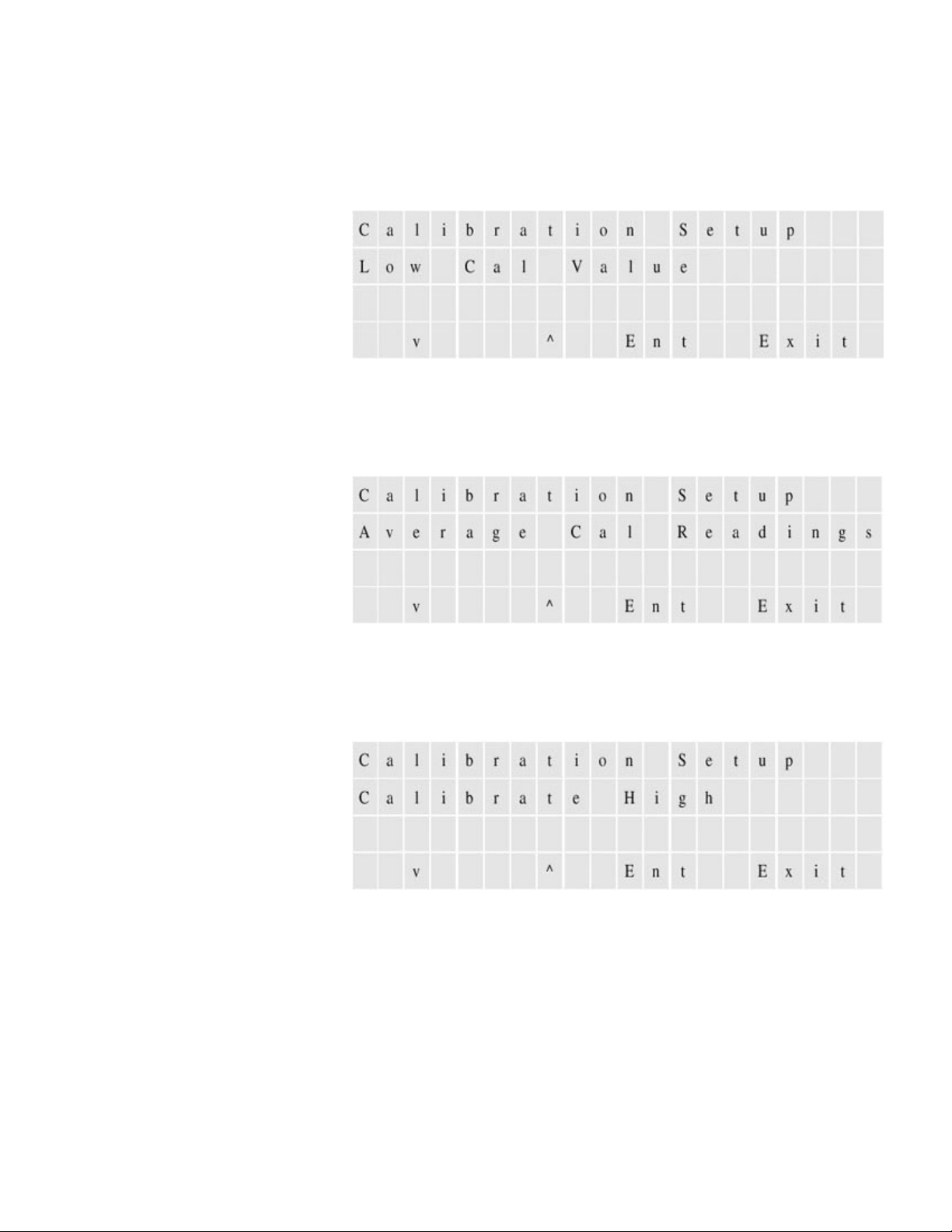
Configuration

Calibration

3. Enter the concentration of the low calibration standard. Note that if using

only one calibration standard and no injections to calibrate the
background, enter zero. See “Performing a Low Calibration at Zero” for
more.

Figure 6–51.

4. Set the number of readings the analyzer should average during calibration

(1–60 readings).

Figure 6–52.

5. Begin a calibration for the high concentration standard. See “Performing a

High Calibration” for more.

Figure 6–53.

Thermo Fisher Scientific SOLA II User Guide 6-23

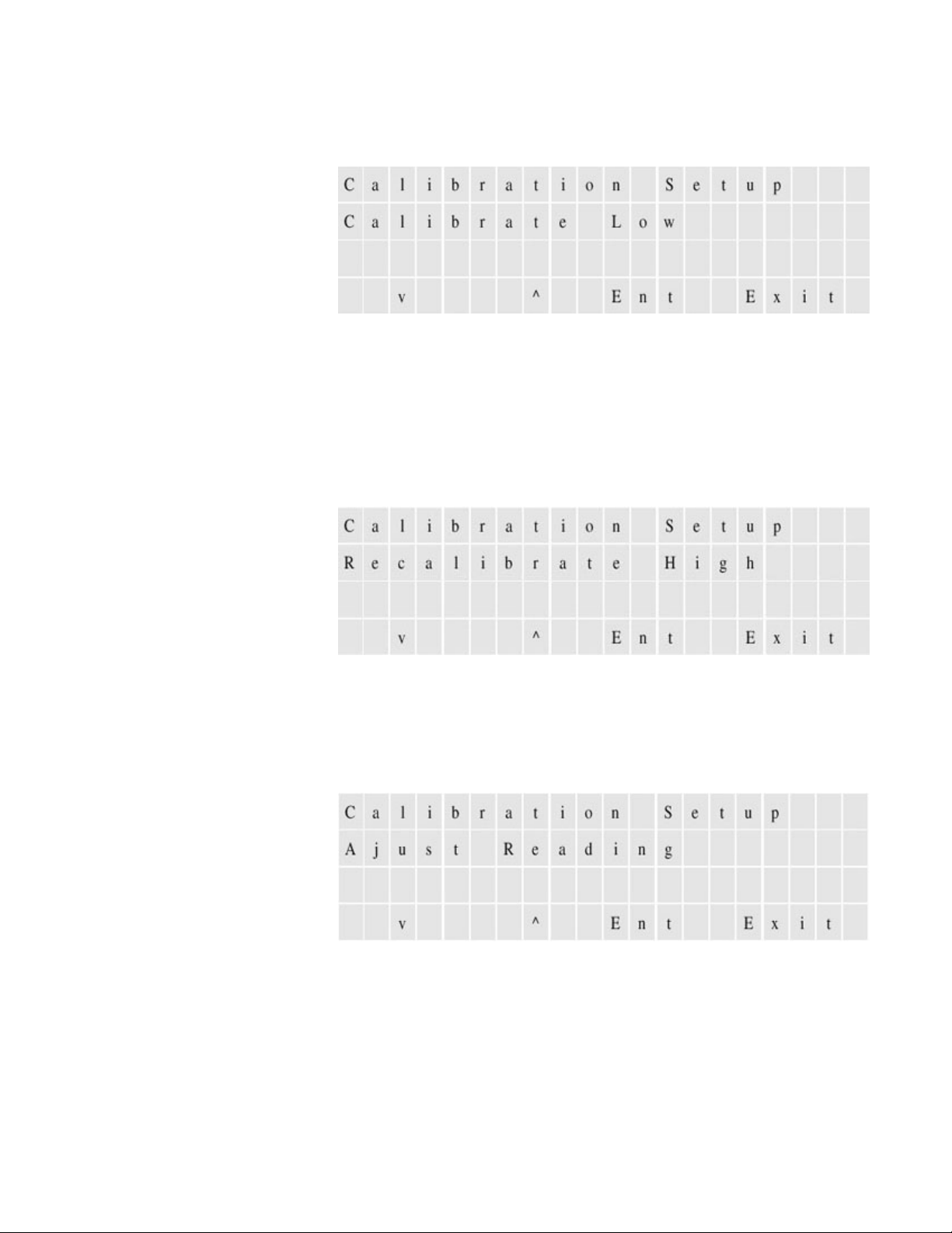
Configuration

Calibration

6. Begin a calibration for the low concentration standard or for zero

background.

Figure 6–54.

7. Perform a calibration without the purge cycle for the high concentration

standard. See “Performing a High Calibration” for more.

You can do the same for the low concentration standard by accessing the
Recalibrate Low menu item (not shown). See “Performing a Low

Calibration at Zero” for more.

Figure 6–55.

8. Adjust calibration during operation to match lab results through the

Adjust Reading menu item. Enter a concentration, and the reading is
forced to match the value entered. See “Adjusting the Reading” for more.

Figure 6–56.

6-24 SOLA II User Guide Thermo Fisher Scientific

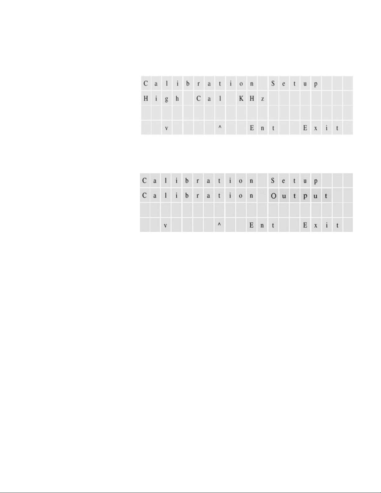
Configuration

Density

nsation

Setup

Density Compensation Setup

9. Review/edit the frequency stored during calibration of the high standard.

You can do the same for the low standard or zero background accessing
the Low Cal KHz menu item.

Figure 6–57.

10. Calibration Output

Compe

Figure 6–58.

Density correction is used for reporting the total sulfur in ppm w/w and can
be accomplished using a density transmitter (densitometer) for each stream
with the output connected to the analyzer’s 4–20 mA inputs or by entering a
fixed correction factor.

When using the optional densitometer inputs, the densities that correspond to
4 mA and 20 mA must be entered. The analyzer maintains a moving average
of the 4–20 mA readings and converts the readings to g/cc using a linear
interpolation. The sulfur reading is then corrected by multiplying it by the
ratio between the calibration sample density and the measured density of the
sample.

When the density of the sample is known and remains relatively constant, a
fixed correction factor can be used. In this method, the total sulfur reading is
multiplied by the value entered. If no correction is desired, set the correction
factor to 1.000.

The following provides instructions for both methods. If using a densitometer,
refer to the instructions with Figures 6–59 through 6–63. Menu items for
stream 1 are used.

Thermo Fisher Scientific SOLA II User Guide 6-25

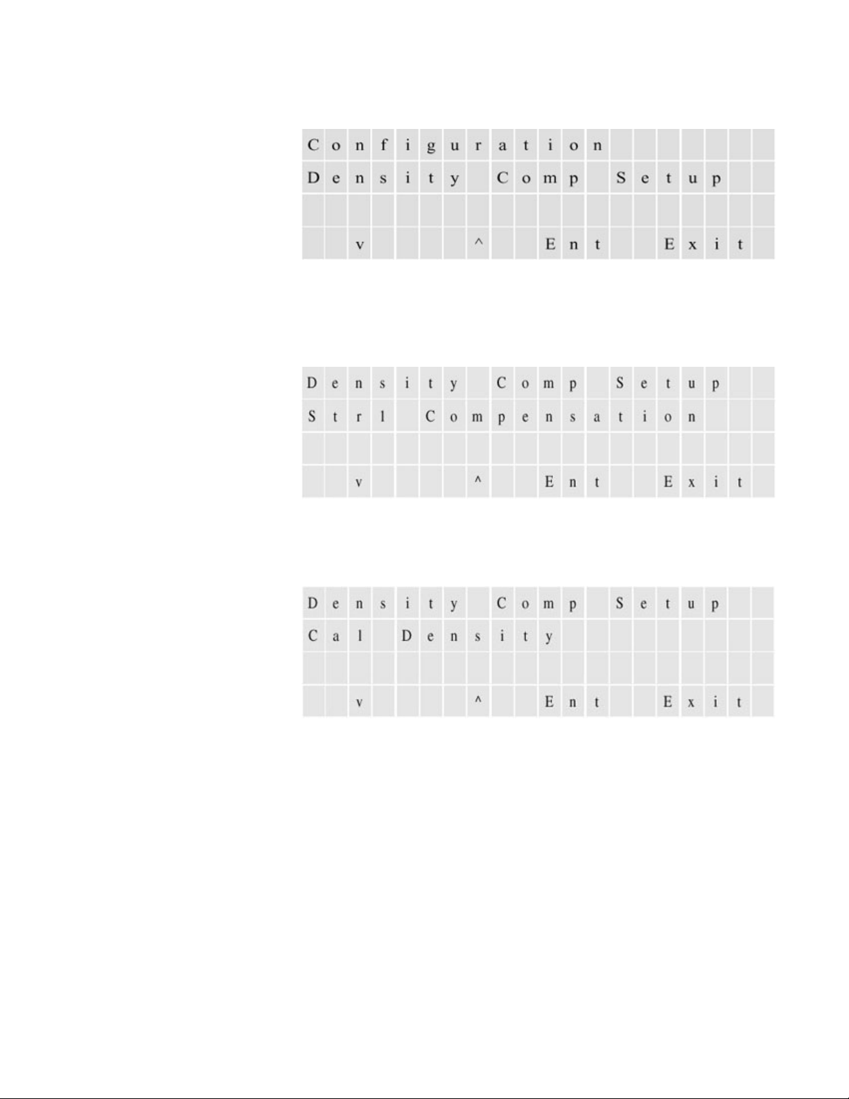
Configuration

Live

Density Compensation Setup

1. Enter the Density Compensation Setup menu.

Figure 6–59.

2. Select

. If you are using stream 2, be sure the menu item is for stream

2.

Figure 6–60.

3. Enter the density of the calibration standard (in units of g/cc).

Figure 6–61.

6-26 SOLA II User Guide Thermo Fisher Scientific

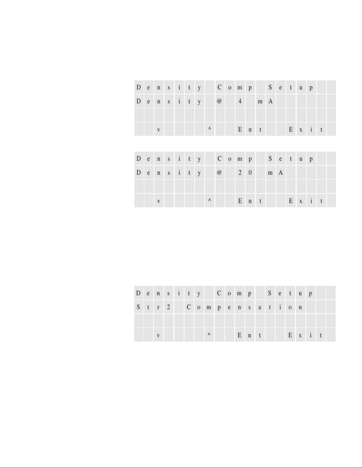
Configuration

Fix

Density Compensation Setup

4. In units of g/cc, enter the density that corresponds to the 4 mA output of

the densitometer used (Figure 6–62). In the following screen (Figure 6–

63), enter the density that corresponds to the 20 mA output of the
densitometer.

Figure 6–62.

Figure 6–63.

The following provides instructions on entering a correction factor using
stream 2.

1. Select

in the Str2 Compensation menu item. If using stream 1, be sure

the menu item is for stream 1.

Figure 6–64.

Thermo Fisher Scientific SOLA II User Guide 6-27

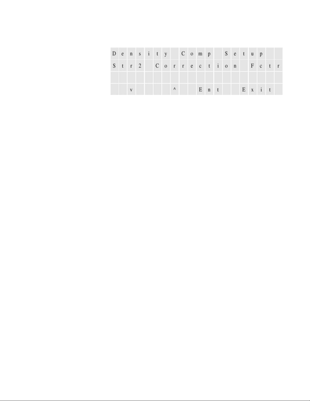
Configuration

Density Compensation Setup

2. Enter the correction factor. The value may be from 0 to 9.999.

Figure 6–65.

Note that when using a correction factor, you do not need to enter the Cal
Density menu.

6-28 SOLA II User Guide Thermo Fisher Scientific

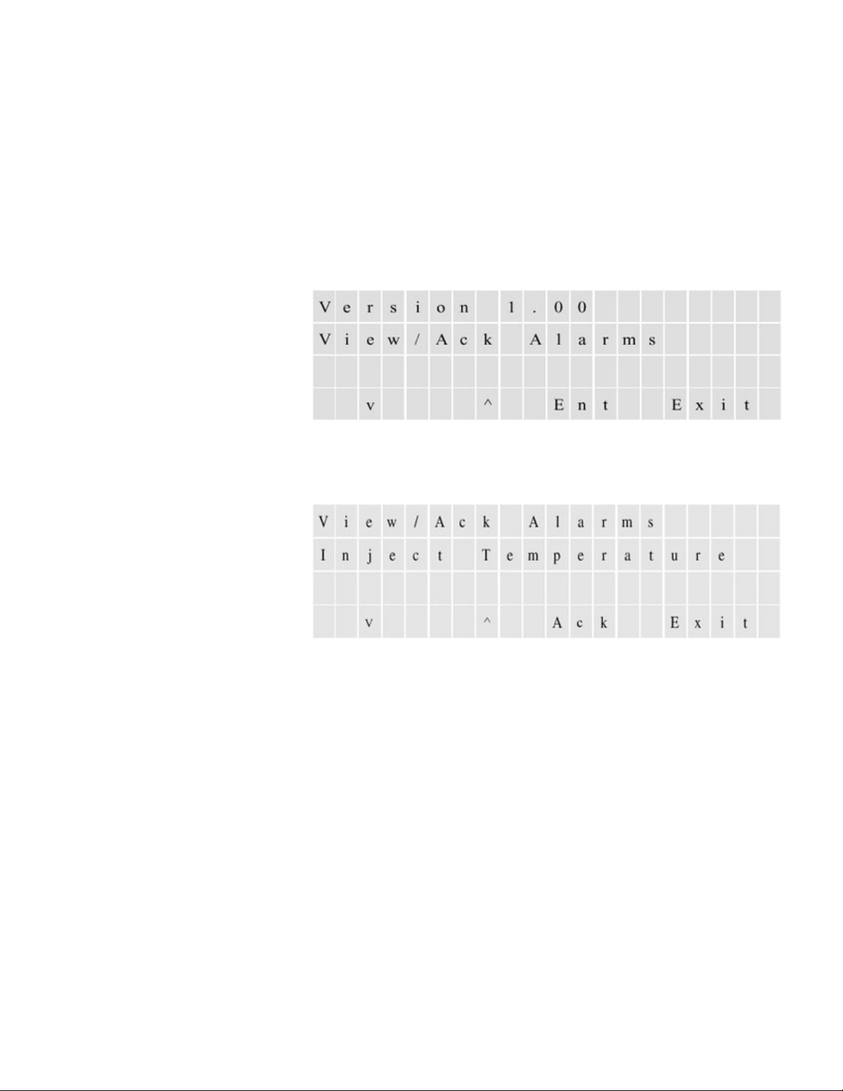
Chapter 7

Ack

Viewing Alarms

The second top-level menu is the View/Ack Alarm menu.

Figure 7–1.

Access this menu to review all active alarms. Use the up and down arrows to
scroll through the alarms individually. Press

Figure 7–2.

to acknowledge the alarm.

Thermo Fisher Scientific SOLA II User Guide 7-1

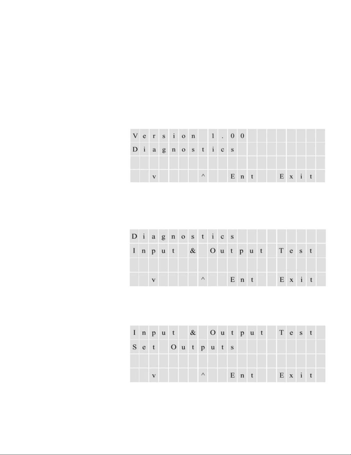
Chapter 8

Tgle

Input & Output

Test Menu

Set Outputs

Diagnostics

There are four submenus within the Diagnostics top-level menu: Input &
Output Test, View Parameters, Com Ports RX TX, Pulse UV Control.

Figure 8–1.

The Input & Output Test menu consists of four groups of submenus: Set
Outputs Menu, View Mux Analogs, 4-20 mA Inputs, and View Digital Inputs.

Figure 8–2.

In the Set Outputs group, press

to toggle the associated relay on and off.

Figure 8–3.

Following are the relays that can be accessed through the Set Outputs group.

Thermo Fisher Scientific SOLA II User Guide 8-1

Diagnostics

View MUX Analogs

Input & Output Test Menu

Table 8–1.

Output Function

Malfunction Malfunction relay (fail safe).
Off Line Denotes calibration cycle or suspended analysis (fail safe).
H Alarm High alarm relay.
HH Alarm High high alarm relay.
Stream Selected Indicates the active stream.
Range Selected
RLY 7 Purge fail (fail safe).
RLY 8 Spare
Stream 1 4–20 mA Press Enter to change the 4–20 mA output for stream 1 to 4, 8, 12,

16, or 20 mA.

Stream 2 4–20 mA Press Enter to change the 4–20 mA output for stream 2 to 4, 8, 12,

16, or 20 mA.
Sample Solenoid Controls the sample diverter.
Stream 1 Solenoid Controls the valve for stream 1.
Stream 2 Solenoid Controls the valve for stream 2.
Inject Solenoid Controls the injection valve.
Cal Solenoid Controls the calibration/stream valve.
Solenoid 6 Controls high/low flow
Solenoids 7–8 See note below
Bench CNTRL ## Reserved for factory test only; the 2 pound signs (##) indicate the

control output.

Note Solenoids 7 and 8 are reserved for future applications and are not

installed in the standard unit. σ

8-2 SOLA II User Guide Thermo Fisher Scientific

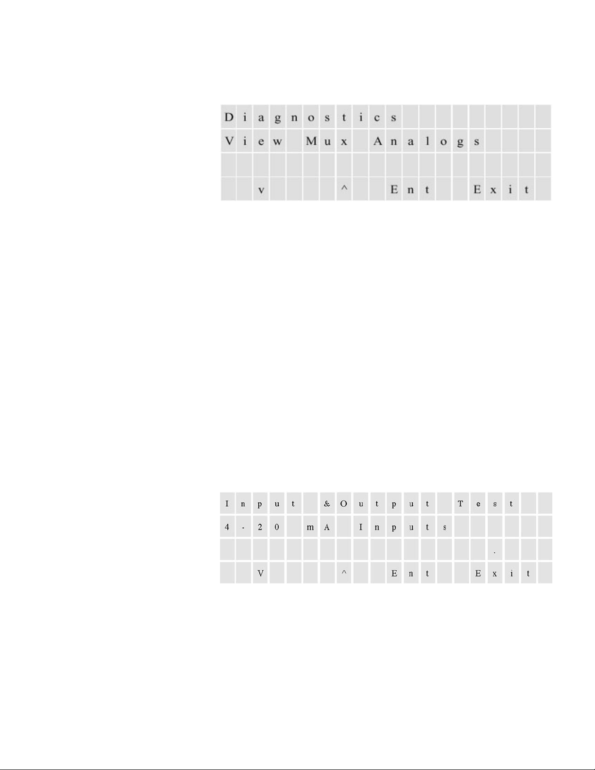
Diagnostics

View 4–20 mA Inputs

Input & Output Test Menu

You can view the MUX analogs by accessing this menu. Note that all signals
are displayed as raw frequencies.

Figure 8–4.

Following are the analogs in the order they appear within menu:

1. ADC 0 Lamp V

2. ADC 1 Chamber Flow

3. ADC 7 Pressure

4. ADC 9 PMT V

5. ADC 10 Chamber T

6. ADC 11 Ambient T

Access this submenu to view the optional 4–20 mA inputs.

Figure 8–5.

Thermo Fisher Scientific SOLA II User Guide 8-3

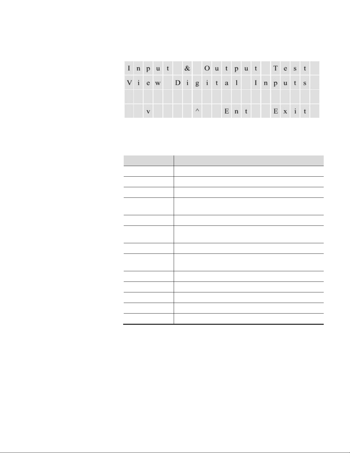
Diagnostics

View Digital Inp ut s

Input & Output Test Menu

When you access the View Digital Inputs menu, the status of the inputs is
reported but the functions are ignored.

Figure 8–6.

Following is a list of inputs and their functions.

Table 8–2.

Input Function

Purge Fail Displays the status of the purge sense pressure switch.
Flow Switch Displays the status of the flow monitoring switch.
Watlow Alarm Displays the status of the Watlow alarm input1
I/O Board Displays the status of all eight inputs simultaneously. Zero (0)

denotes open. One (1) denotes closed.
CPU Digital In
Dip Switches Displays the positions of dip switches located in the motherboard (dip

switches are used to indicate options installed)
I/O Board Option
4–20 mA Input

Option
Stream Select 1 Displays the status of stream select switch #1
Stream Select 2 Displays the status of stream select switch #2
Range Control Displays the status of the range control switch
Remote Cal Displays the status of the remote calibration switch
Remote Suspend Displays the status of the remote suspend switch

8-4 SOLA II User Guide Thermo Fisher Scientific

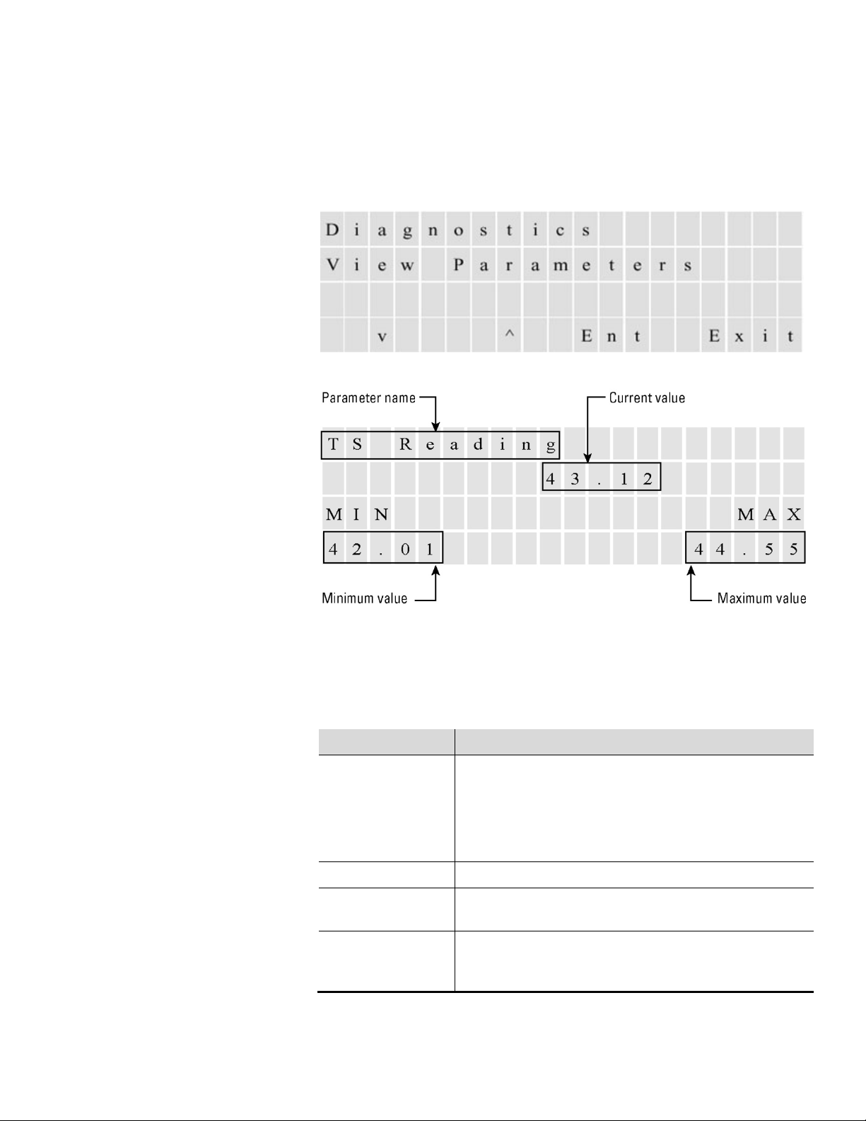
Diagnostics

View Parameters

View Parameters

Each menu item within the View Parameters menu displays the parameter
name, current value, minimum value, and maximum value (see Figure
8–8). When you select a parameter to view, the minimum and maximum
values are reset to the current value. Displaying the minimum, maximum, and
current values for a period of time enables you to monitor signal stability.

Figure 8–7.

Figure 8–8.

Following are the menu items within the View Parameters menu.

Table 8–3.

Menu Item Description

At line sample Access this item to view the latest at line sample results:

Sample AVG: The Average Concentration of the sample.
SD: The Standard Deviation computed during the average.
% RSD: The Relative Standard Deviation computed as a

percentage of the average.
TS Reading The concentration reading.
Response Factors The slope (kHz/ppm or kHz/ppb sensitivity) and the offset

(calculated at 0 concentration).

Working Average Sec When switching from the normal average to the fast average and

back to normal, the average time used can be observed from this
menu item.

Thermo Fisher Scientific SOLA II User Guide 8-5

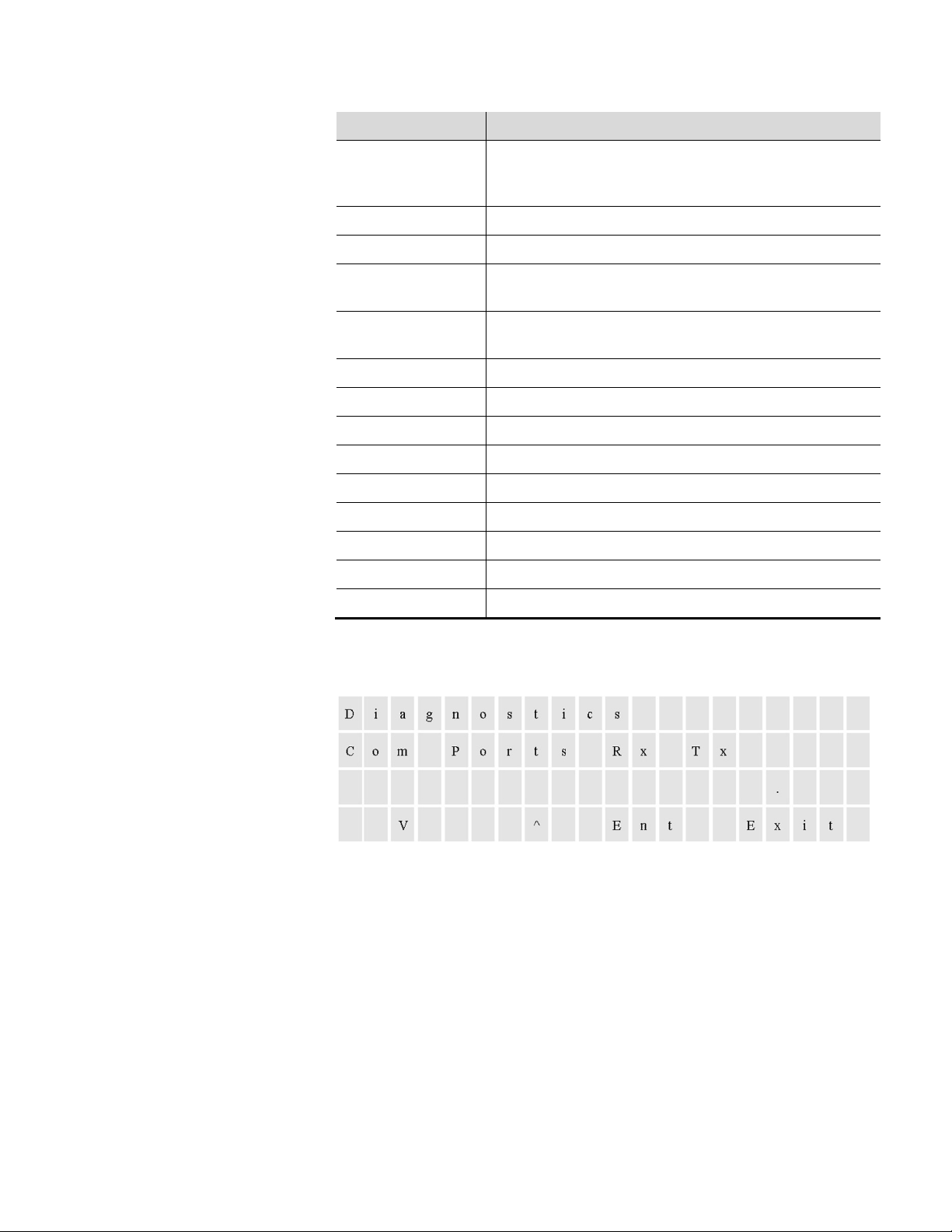
Diagnostics

View Com

Activity

View Com Activity

Menu Item Description

% of Deviation The percentage of deviation of the most current reading with

respect to the average. This is the value used to switch to the fast

average.
Rate of Change ppm/s The rate of change of the sulfur reading expressed as ppm/sec.
AVG PMT signal kHz The average of the raw detector signal.
Normalized PMT kHz The frequency proportional to the PMT output normalized to the

gain of 100; also displays the gain currently selected.
PMT Signal kHz The actual frequency proportional to the PMT output; also displays

the gain currently selected.
PMT Voltage The input voltage to the PMT.
Internal Temperature The temperature inside the electronics enclosure.
Chamber Temperature The temperature inside the reaction chamber.
Chamber Flow The flow through the reaction chamber.
Chamber Pressure The pressure sensed at the reaction chamber.
Lamp Intensity The frequency proportional to the lamp intensity.
Lamp Voltage The lamp input voltage.
Stream 1 Density The density of stream 1.
Stream 2 Density The density of stream 2.

This menu displays activity for Coms 1–4.

Figure 8–9.

8-6 SOLA II User Guide Thermo Fisher Scientific

Diagnostics

Pulse UV Control

Pulse UV Control

Following are the menu items within the Pulse UV Control menu.

Caution This menu is intended for factory test only. Incorrect settings can

result in damage to the unit. σ

Table 8–4.

Menu Item Description

Flash Lamp ON/OFF Turn the UV lamp flashing on or off.
Auto Gain ON/OFF Turn the amplifier auto gain selection on or off.

Note Auto gain defaults to ON during normal operation.

PMT Signal Gain Select the amplifier gain (1, 2, 5, 10, 20, 50, 100).

Note The selection is only valid when auto gain is turned

σ

OFF.

Test Gains Place the gain selection under manual control to verify the

functionality of the programmable gain amplifier.

Test LED ON/OFF Test the LED by turning it on and off.

σ

Flash Frequency Change the UV lamp flash frequency (normally 10 Hz).
Flash Time Change the duration of the flashing pulse (normally 100 µs).
S&H Time (Sample &

Hold Time)

Change the duration of the sample portion of the sample and hold
analog front end (normally 100 µs). (Sample portion is the amount
of time the sample and hold device is in the SAMPLE state.)

Thermo Fisher Scientific SOLA II User Guide 8-7

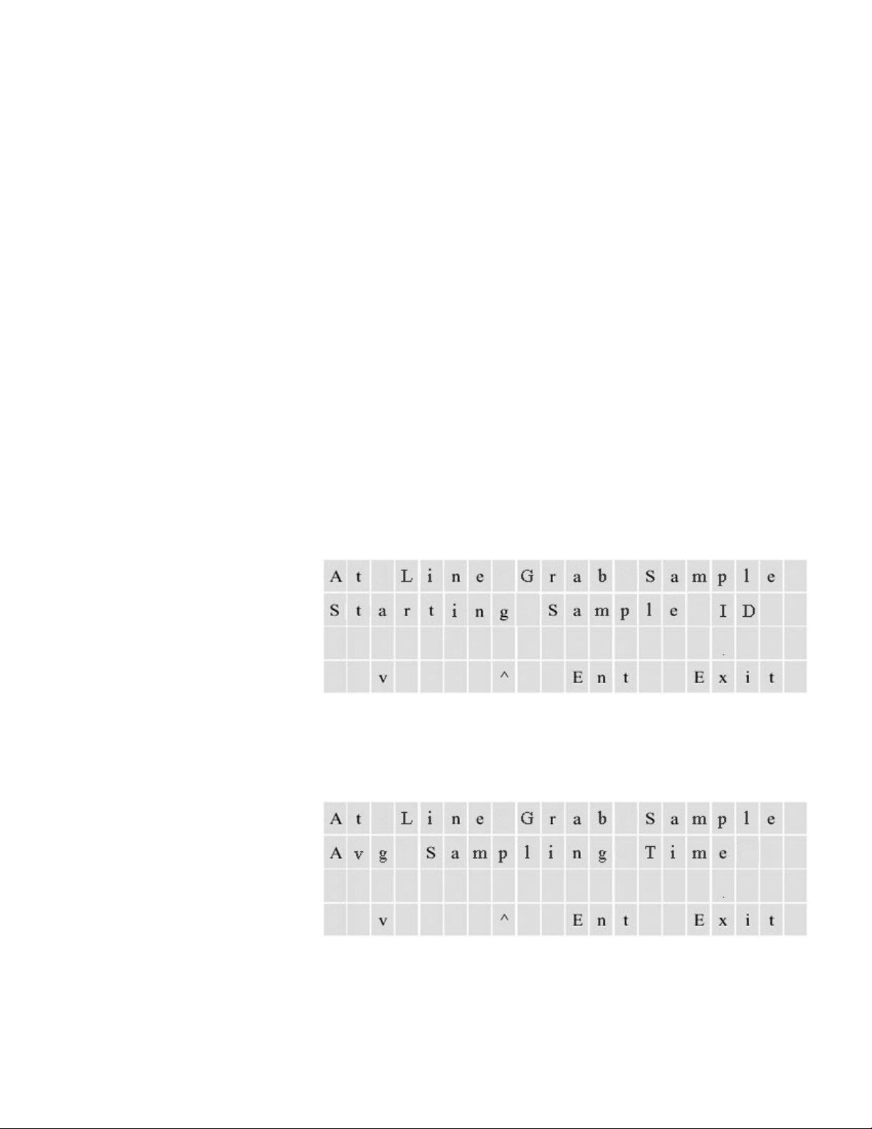
Chapter 9

At Line-Grab Sample

This function was developed primarily for pipeline applications. The sampling
system was designed for the pipeline enclosure in order to provide an
additional pump to facilitate introduction of sample. Access this top-level
menu to enable the analyzer to analyze and report the results of a sample
previously collected from a source other than the regular process input. The
sample to be analyzed is introduced into the instrument in the same manner
that a calibration standard is.

There are three parameters to configure: starting sample ID, average sampling
time, and the relative standard deviation of the samples taken.

1. Each sample is identified with a number (starting sample ID). The

numbers increment sequentially until a new starting sample ID is
programmed.

Figure 9–1.

2. Average sampling time is the number of seconds that the sample is

averaged to compute the result. It can be between 60 and 240 seconds.

Figure 9–2.

Thermo Fisher Scientific SOLA II User Guide 9-1

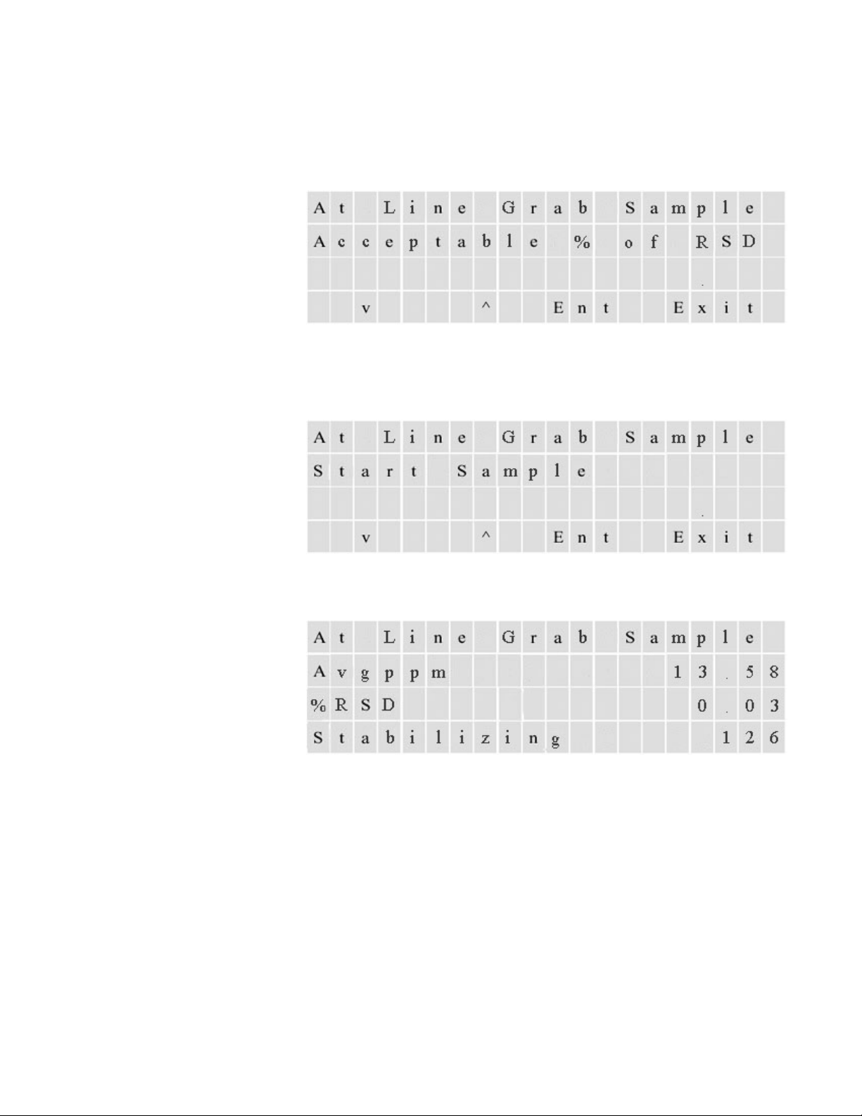
At Line-Grab Sample

3. The relative standard deviation (RSD) of the samples taken is computed

as a percentage of the computed average. If it is less than or equal to the
programmed value, the analyzer reports a successful sample. If it is
greater than the programmed value, an error is reported.

Figure 9–3.

Activate the function from the front panel or the SOLA web interface.

Figure 9–4.

Figure 9–5. At line sampling screen

9-2 SOLA II User Guide Thermo Fisher Scientific

Chapter 10

Safety

Precautions

Maintenance

Schedule

Maintenance & Tr oubl eshooting

Caution Some internal components can be damaged by small amounts of

static electricity. Take appropriate precautions (use a properly grounded
antistatic wrist strap) when handling electronic boards and components.

To avoid damaging internal components, follow these precautions when
performing any service procedure:

λ Wear an antistatic wrist strap that is properly connected to earth ground.

If an antistatic wrist strap is not available, be sure to touch a grounded
metal object before touching any internal components.

λ Handle all printed circuit boards by the edges.

λ Carefully observe the instructions in each procedure. σ

Table 10–1. Maintenance schedule

Frequency Tasks

Monthly Calibrate the analyzer (Chapter 6).
Every six months Visually inspect and clean the instrument.

Check the instrument flow rates as explained later in this chapter.
Replace the injection valve rotor or slider according to Appendix B.

Annually Test the instrument for internal leaks as explained later in this

chapter.

Every 18 months Replace the pyrolyzer heater as explained later in this chapter.

Thermo Fisher Scientific SOLA II User Guide 10-1

Maintenance & Troubleshooting

Visual Inspection &

Cleaning

Leak Tests

Visual Inspection & Cleaning

The analyzer should be inspected occasionally for obvious visible defects, such
as loose connectors, loose fittings, cracked or clogged Teflon lines, and
excessive dust or dirt accumulation. Dust and dirt can accumulate in the
instrument and can cause overheating or component failure. Dirt on the
components prevents efficient heat dissipation and may provide conducting
paths for electricity.

Warning Remove all instrument power before cleaning electronics. σ

The best way to clean the inside of the instrument is to first carefully vacuum
all accessible areas and then blow away the remaining dust with low-pressure
compressed air. Use a soft paintbrush or cloth to remove stubborn dirt.

Use the following leak test procedure to verify that there are no system leaks.

1. Set the sample and air regulators for zero pressure.

2. Replace the tubing from the EXHAUST bulkhead on the left side of the
instrument with a plug.

3. Adjust the auxiliary air regulator for 20 psig pressure.

4. Turn the auxiliary air regulator fully counterclockwise to close the supply
flow.

5. Watch the analyzer pressure for 15 minutes.

6. If the pressure drops significantly, perform the following to locate the
leak:

a. Adjust the sample and air regulators for 20 psig pressure.

b. Check the system fittings with a liquid or electronic leak detector.

c. Correct any leakage.

d. Repeat the leak test.

10-2 SOLA II User Guide Thermo Fisher Scientific

7. When the system passes the leak test, adjust the sample and air regulators
fully counterclockwise to close supply flows.

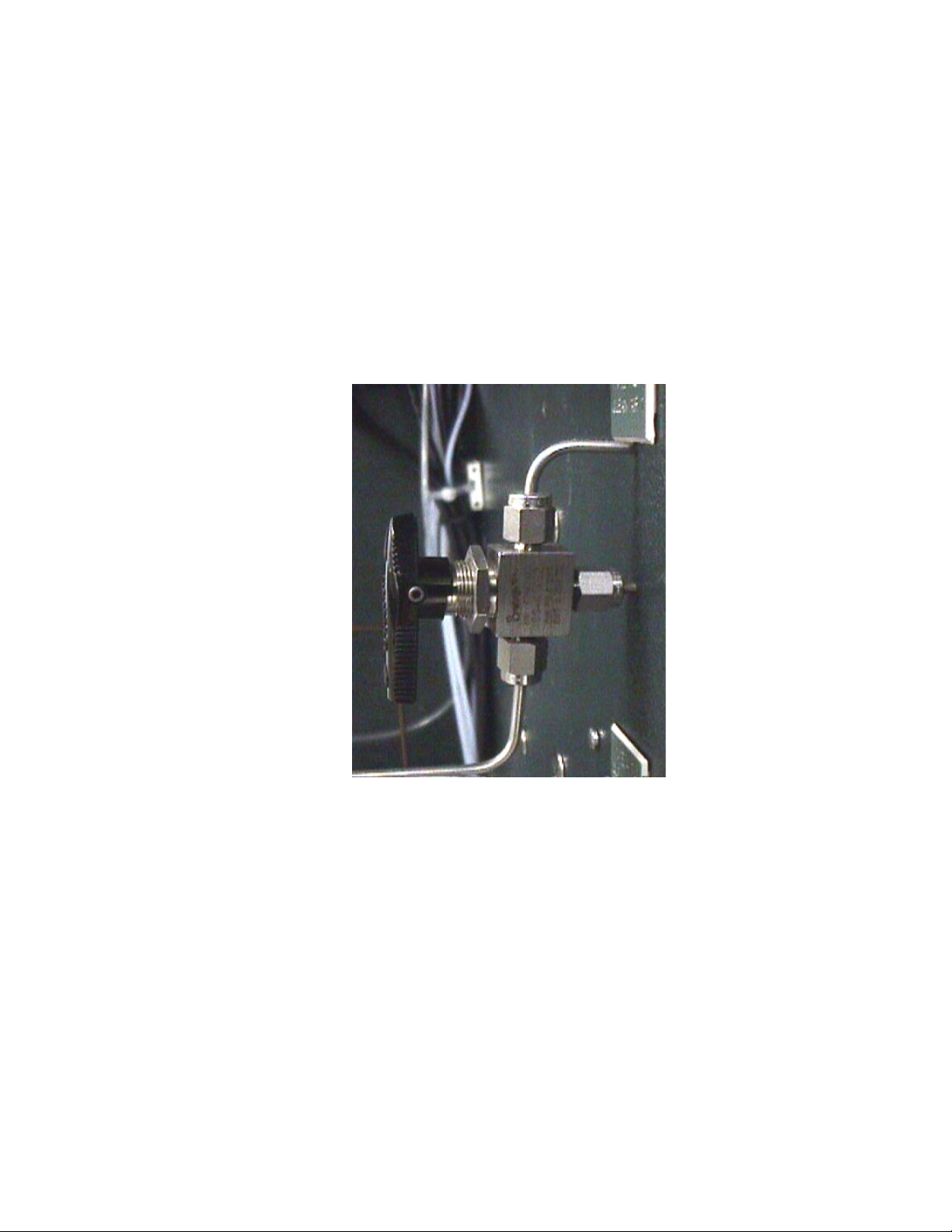
Maintenance & Troubleshooting

Flow Rate

Checks

Flow Rate Checks

8. Remove the plug from the EXHAUST bulkhead and reconnect the

EXHAUST vent line.

9. Adjust the sample and air regulators to the pressures specified in the

application notes shipped with the instrument or as recorded in the
instrument logbook.

10. Allow the analyzer to warm up until it stabilizes.

Figure 10–1. Three-way valve for measuring flow rates

1. Obtain a precision flow measurement instrument such as a bubble meter.

2. Ensure that all pressure regulators are set to the correct pressures as

shown on the calibration data shipped with the instrument or as recorded
in the instrument logbook.

3. Ensure that the analyzer is stabilized at normal operating temperatures

before proceeding.

4. Suspend the analyzer according to Chapter 5.

Thermo Fisher Scientific SOLA II User Guide 10-3

Maintenance & Troubleshooting

The Rotary Valve

The Mixing

Chamber

The Rotary Valve

5. Turn the MEAS. CLEAN AIR 1 3-way valves to point down for flow
measurement.

6. Connect the flow meter to the MEAS. CLEAN AIR 1 port and adjust the

CLEAN AIR 1 regulator to obtain the required flow.

7. Turn the MEAS. CLEAN AIR 1 3-way valves to point up for normal
operation.

8. Turn the MEAS. CLEAN AIR 2 3-way valves to point down for flow
measurement.

9. Connect the flow meter to the MEAS. CLEAN AIR 2 port and adjust the
CLEAN AIR 2 regulator to obtain the required flow.

10. Turn the MEAS. CLEAN AIR 2 3-way valves to point up for normal
operation.

11. Restart the analyzer according to Chapter 5.

For detailed instructions on maintaining, removing, and replacing the rotary
valve, refer to Appendix B.

1. Shut down the system according to Chapter 4.

2. Loosen the fittings that connect the tubing to the mixing chamber.

3. Loosen the screw located in the center of the bracket holding the mixing
chamber to the bottom of the enclosure.

4. Carefully slide the mixing chamber from the bracket.

Note Install the mixing chamber by following the above steps in reverse. σ

10-4 SOLA II User Guide Thermo Fisher Scientific

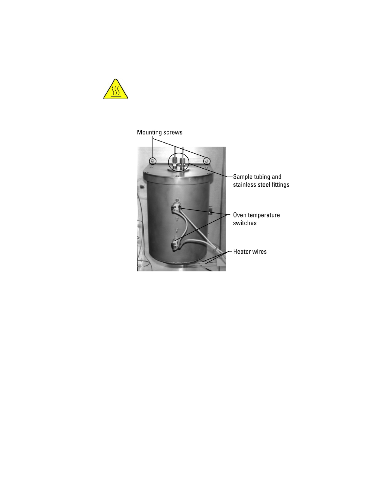
Maintenance & Troubleshooting

Replacing the

Pyrolyzer Heater

Replacing the Pyrolyzer Heater

Warning The pyrolyzer can be extremely hot, even after power is turned off.

Use extreme care to prevent burns! σ

The pyrolyzer heater is enclosed in the pyrolyzer housing, which is shown in
the figure below.

Figure 10–2. Pyrolyzer housing

The following table lists the part numbers for the parts referenced in this
procedure. With the exception of the heater being replaced, the existing parts
can be reused if in good condition. The part numbers are provided here for
convenience.

Thermo Fisher Scientific SOLA II User Guide 10-5

Maintenance & Troubleshooting

Replacing the Pyrolyzer Heater

Table 10–2. Parts list for heater replacement

P/N Qty. Description

27-1108-0 1 Thermocouple, S-type
29-1230-0 1 Heater, fiber insulated, 60 V/450 W
29-1231-0 1 Insulation, flameless burner
30-1025-0 1 Pyrolyzer tube, looped
40-0025 0.5 ft2 Kaowool® insulation
56-1074-0 1 Terminal, 2 pole ceramic block, 30 A
64-1301-0 2 Heater wire sleeve, flameless burner
65-1041-0 1 ft Insulation, fiberglass
68-1269-2 2 Red SS, 1Tx4T
89-2917-0 1 Pyrolyzer, tested assembly (includes housing, housing

lid, O-ring, screws, washers)

HA-101812 2 Ferrule, 1/4 graphite

1. Follow the maintenance shutdown procedure in Chapter 4 to shut down
the analyzer system. Allow the system to cool completely.

2. Carefully remove the two sample tubes from the top of the pyrolyzer
housing using a backup wrench to keep the stainless steel fittings from
turning.

3. Loosen the terminal block screws and disconnect the thermocouple wires.
Be sure to note the orientation of the wire colors.

4. If installed, disconnect the wires from the oven temperature switches; the
wire between the two sensors can be left in place.

5. Slightly loosen the two screws that attach the bottom of the housing to
the back of the oven.

6. Support the housing while removing the top two mounting screws that
hold it to the back of the oven. After both screws have been removed, lift
the pyrolyzer up and out of the oven. Do not discard the mounting
screws. You will need them later.

7. Remove the six screws and washers from the lid of the housing (Figure 10-

3). Set them aside for later use.

10-6 SOLA II User Guide Thermo Fisher Scientific