Teledyne LeCroy WaveSurfer 3034, WaveSurfer 3022, WaveSurfer 3024, WaveSurfer 3054 Operator's Manual

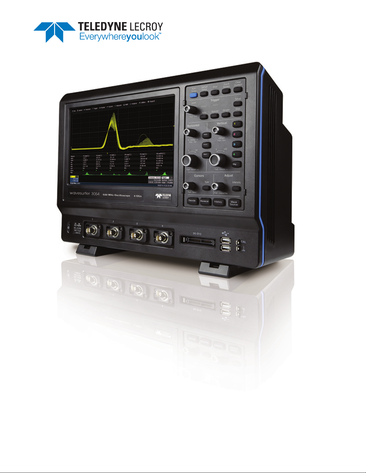
Operator's Manual

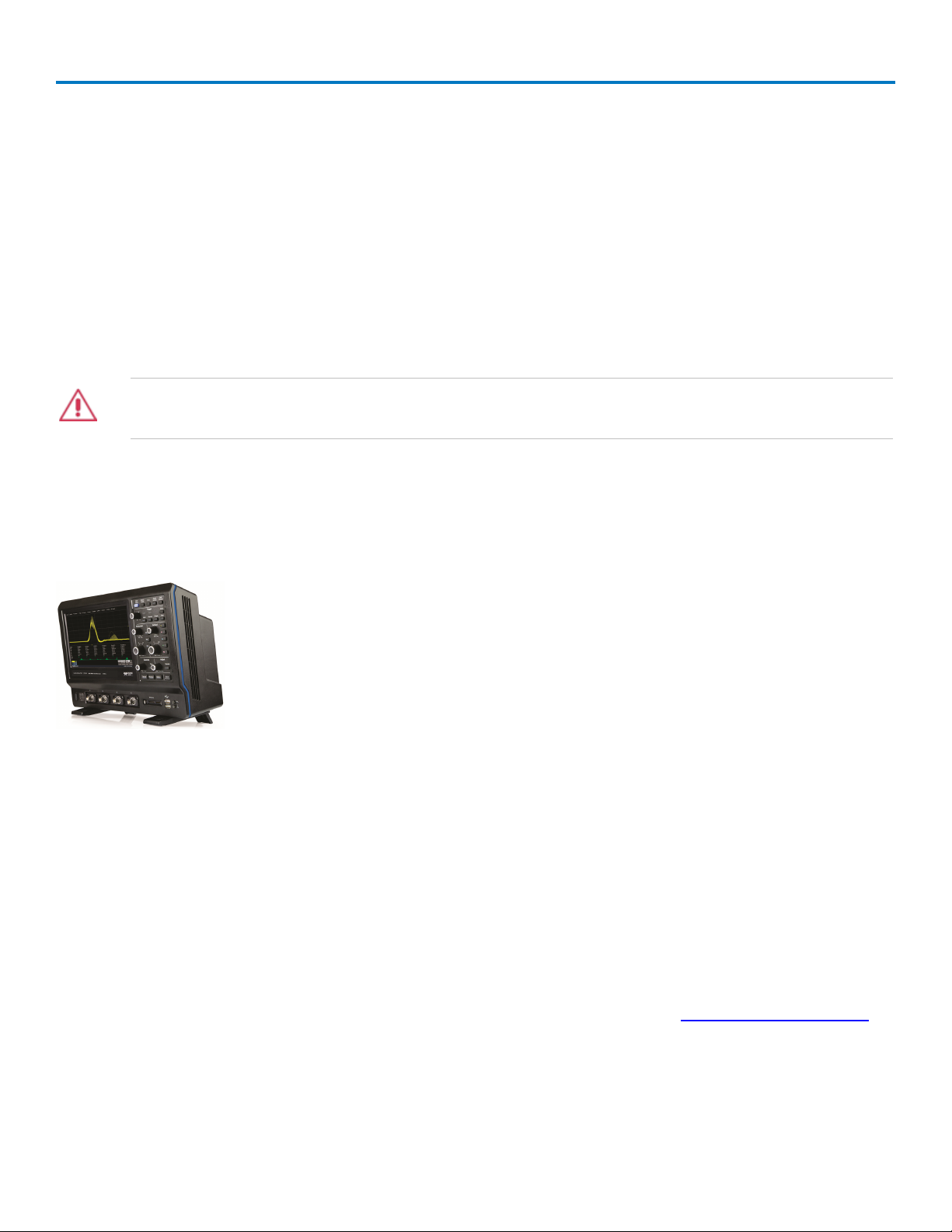
WaveSurfer 3000 Oscilloscopes

WaveSurfer 3000 Oscilloscopes Operator's Manual

Unauthorized duplication of Teledyne LeCroy documentation materials other than for internal sales and distribution purposes is strictly prohibited. However, clients are encouraged to distribute and duplicate Teledyne LeCroy documentation for their own internal educational purposes.

WaveSurfer and Teledyne LeCroy are trademarks of Teledyne LeCroy, Inc. Other product or brand names are trademarks or requested trademarks of their respective holders. Information in this publication supersedes all earlier versions. Specifications are subject to change without notice.

923648 Rev B November 2014

Operator's Manual

Contents

Safety Instructions 1

Symbols 1 Precautions 1 Operating Environment 2 Cooling 2 Power 2

Start Up 4

Setting Up the Oscilloscope 4 Powering On/Off 5 Software Activation 6

Inputs/Outputs 7

Front Input/Output Panel 7 Back Input/Output Panel 7 Analog Inputs 8 Probes 8 Digital Inputs 8

Touch Screen 10

Menu Bar 10 Signal Display Grid 11 Descriptor Boxes 12 Dialogs 14 Turning On/Off Traces 15 Annotating Traces 16 Entering/Selecting Data 17 Print Preview 19 Printing/Screen Capture 20 Language Selection 20

Front Panel 21

Top Row Buttons 21 Trigger Controls 21 Horizontal Controls 22 Vertical Controls 22 Math, Zoom, and Mem(ory) Buttons 22 Cursor Controls 22 Adjust and Intensity Controls 23 Bottom Row Buttons 23

Zooming Waveforms 24

Creating Zooms 24 Zoom Controls 25

Vertical 26

Channel Settings 26

WaveSurfer 3000 Oscilloscopes

Probe Settings 27 Auto Setup 28 Restore Default Setup 28 Viewing Status 29

Digital (Mixed Signal) 30

Digital Traces 30 Digital Group Set Up 30 Digital Display Set Up 31 Renaming Digital Lines 32

Timebase 33

Timebase Settings 33 Sampling Modes 34 History Mode 38

Trigger 40

Trigger Modes 40 Trigger Types 41 Setting UpTriggers 42 Trigger Holdoff 58

Display 60

Display Settings 60 Persistence 61

Cursors 63

Cursor Types 63 Cursor Settings 64

Measure 65

Setting Up Measurements 65 List of Standard Measurement Parameters 67 Calculating Measurements 69

Math 71

Setting Up Math Functions 71 List of Standard Math Functions 73 Trend 74 Rescaling and Assigning Units 75 Averaging Waveforms 77 FFT 78

Memory 81

Save Waveform to Memory 81 Restore Memory 81

Analysis 82

WaveScan 82

Utilities 86

System Status 86

Operator's Manual

Remote Control Settings 87 Hardcopy Settings 90 Aux Output Settings 92 Date/Time Settings 92 Options 93 Preferences Settings 93 Calibration Settings 94 Acquisition Settings 95 E-Mail 95 Miscellaneous Settings 96 Digital Voltmeter 97 WaveSource Automatic Waveform Generator 99

Save/Recall 101

Save/Recall Setups 101 Save/Recall Waveforms 103 Save Table Data 106 Auto Save 107 Disk Utilities 107

LabNotebook 109

Create Notebook Entry 109 Print to Notebook Entry 110 Flashback Recall 110 Configure LabNotebook Preferences 111

Maintenance 112

Cleaning 112 Fuse Replacement 112 Calibration 112 Touch Screen Calibration 113 Reboot Oscilloscope 113 Adding an Option Key 113 WaveSurfer 3000 Firmware Update 114 Technical Support 114 Returning a Product for Service 115

Certifications 117

EMC Compliance 117 Safety Compliance 118 Environmental Compliance 119 ISO Certification 119

Warranty 120

iii

WaveSurfer 3000 Oscilloscopes

Welcome

Thank you for purchasing a Teledyne LeCroy WaveSurfer Oscilloscope. We're certain you'll be pleased with the detailed features unique to our instruments.

The manual is arranged in the following manner:

l Safety contains important precautions and information relating to power and cooling.

l The sections from Start Up through Maintenance cover everything you need to know about the

operation and care of the oscilloscope.

Documentation for software options is available from the Teledyne LeCroy website at teledynelecroy.com. Our website maintains the most current product specifications and should be checked for frequent updates.

Remember...

When your product is delivered, verify that all items on the packing list or invoice copy have been shipped to you. Contact your nearest Teledyne LeCroy customer service center or national distributor if anything is missing or damaged. We can only be responsible for replacement if you contact us immediately.

Thank You

We truly hope you enjoy using Teledyne LeCroy's fine products.

Sincerely,

David C. Graef

Teledyne LeCroy

Vice President and Chief Technology Officer

Operator's Manual

Safety Instructions

Observe these instructions to keep the instrument operating in a correct and safe condition. You are required to follow generally accepted safety procedures in addition to the precautions specified in this section. The

overall safety of any system incorporating this instrument is the responsibility of the assembler of the system.

Symbols

These symbols appear on the instrument's front and rear panels or in its documentation to alert you to important safety considerations:

CAUTION of potential damage to instrument, or WARNING of potential bodily injury. Do not proceed until the information is fully understood and conditions are met.

High voltage. Risk of electric shock or burn.

Ground connection.

Alternating current.

Standby power (front of instrument).

Precautions

Use only the proper power cord shipped with this instrument and certified for the country of use.

Maintain ground. This product is grounded through the power cord grounding conductor. To avoid electric

shock, connect only to a grounded mating outlet.

Connect and disconnect properly. Do not connect/disconnect probes or test leads while they are connected to a voltage source.

Observe all terminal ratings. Do not apply a voltage to any input (C1-C4 or EXT) that exceeds the maximum rating of that input. Refer to the front of the oscilloscope for maximum input ratings.

Use only within operational environment listed. Do not use in wet or explosive atmospheres.

Use indoors only.

Keep product surfaces clean and dry. See Cleaning in the Maintenance section.

Do not block the cooling vents. Leave a minimum six-inch (15 cm) gap between the instrument and the

nearest object.

Do not remove the covers or inside parts. Refer all maintenance to qualified service personnel.

WaveSurfer 3000 Oscilloscopes

Do not operate with suspected failures. Do not use the product if any part is damaged. Obviously incorrect measurement behaviors (such as failure to calibrate) might indicate impairment due to hazardous live electrical quantities. Cease operation immediately and sequester the instrument from inadvertent use.

Operating Environment

Temperature: 0 to 50° C.

Humidity: Maximum relative humidity 90 % for temperatures up to 31° C, decreasing linearly to 50% relative

humidity at 40° C.

Altitude: Up to 3,000 m at or below 30° C.

Cooling

The instrument relies on forced air cooling with internal fans and vents. Take care to avoid restricting the airflow to any part. Around the sides and rear, leave a minimum of 15 cm (6 inches) between the instrument and the nearest object. The feet provide adequate bottom clearance.

CAUTION. Do not block cooling vents. Always keep the area beneath the instrument clear of paper and other items.

The instrument also has internal fan control circuitry that regulates the fan speed based on the ambient temperature. This is performed automatically after start-up.

Power

The instrument operates from a single-phase, 100 to 240 Vrms (± 10%) AC power source at 50/60 Hz (± 5%), or a 100 to 120 Vrms (± 10%) AC power source at 400 Hz (± 5%). The instrument automatically adapts to the line voltage. Manual voltage selection is not required.

The AC inlet ground is connected directly to the frame of the instrument. For adequate protection again electric shock, connect to a mating outlet with a safety ground contact.

WARNING. Interrupting the protective conductor inside or outside the oscilloscope, or disconnecting the safety ground terminal, creates a hazardous situation. Intentional interruption is prohibited.

Maximum power consumption with all accessories installed (e.g., active probes, USB peripherals, digital leadsets) is 150 W (150 VA) for fourchannel models and 100 W (100 VA) for two-channel models. Power consumption in standby mode is 4 W.

AC Power

The instrument operates from a single-phase, 100 to 240 Vrms (± 10%) AC power source at 50/60 Hz (± 5%), or a 100 to 120 Vrms (± 10%) AC power source at 400 Hz (± 5%) . Manual voltage selection is not required because the instrument automatically adapts to the line voltage.

Operator's Manual

Power Consumption

Maximum power consumption with all accessories installed (e.g., active probes, USB peripherals, digital leadset) is 150 W (150 VA) for four-channel models and 100 W (100 VA) for two-channel models. Power consumption in standby mode is 4 W.

Ground

The AC inlet ground is connected directly to the frame of the instrument. For adequate protection again electric shock, connect to a mating outlet with a safety ground contact.

WARNING. Only use the power cord provided with your instrument. Interrupting the protective conductor inside or outside the oscilloscope, or disconnecting the safety ground terminal, creates a hazardous situation. Intentional interruption is prohibited.

Fuse Replacement

Disconnect the power cord before inspecting or replacing the fuse. Open the fuse holder (located at the rear of the instrument below the AC power inlet) using a small, flat-bladed screwdriver. Replace the old fuse with a new 5 x 20 mm T-rated 3 A/250 V fuse. Close the fuse holder before powering on.

WARNING. For continued fire protection at all line voltages, replace the fuse with one of the specified type and rating only. Always disconnect the power cord before replacing the fuse.

WaveSurfer 3000 Oscilloscopes

Start Up

Setting Up the Oscilloscope

Carrying and Placing the Oscilloscope

The oscilloscope’s case contains a built-in carrying handle. Grasp the handle firmly and lift the instrument. Always unplug the instrument from the power source before lifting and carrying it.

Place the instrument where it will have a minimum 15 cm (6 inch) clearance from the nearest object. Be sure there are no papers or other debris beneath the oscilloscope or blocking the cooling vents.

CAUTION. Do not place the instrument so that it is difficult to reach the power cord in case you need to quickly disconnect from power.

Positioning the Feet

The WaveSurfer is equipped with rotating, tilting feet to allow four different viewing positions.

To tilt the body back slightly for bench top viewing, pull the small flaps on the bottom of the feet away from the body of the oscilloscope.

To tilt the body forward, rotate both feet to the back. This position is useful when placing the oscilloscope on a high shelf. Pulling out the flaps in this position increases the angle of the tilt.

Connecting to Other Devices/Systems

Make the desired cable connections. All except for the power connection are optional.

After start up, configure the connection on the oscilloscope using the menu options listed below. More detailed instructions are provided later in this manual.

LAN

WaveSurfer 3000 accepts DHCP network addressing. Connect a cable from either Ethernet port on the back panel to a network access device. Go to Utilities > Utilities Setup > Remote and select TCPIP to obtain a network connection and IP address. Go to Utilities > Preference Setup > Email to configure email settings.

USB PERIPHERALS

Connect USB-peripherals (e.g., mouse, keyboard) to any USB port on the front or back of the instrument.

Operator's Manual

EXTERNAL MONITOR

WaveSurfer 3000 supports external monitors with 1024 x 600 ppi resolution. Connect the monitor cable to the VGA video output on the back of the instrument. The connection is “plug-and-play” and does not require any further configuration on the oscilloscope. If necessary, configure the monitor to receive output.

PRINTER

WaveSurfer 3000 supports PictBridge-compliant printers. Connect the printer to any host USB port. The connection is "plug-and-play."

EXTERNAL CONTROLLER

Connect a USB-A/B cable from the USBTMC port or an Ethernet cable from the LAN port on the back of the instrument to the controller. Go to Utilities > Utilities Setup > Remote to configure remote control.

OTHER AUXILIARY DEVICE

To send trigger out to another device, connect a BNC cable from Aux Out on the back of he instrument to the other device.

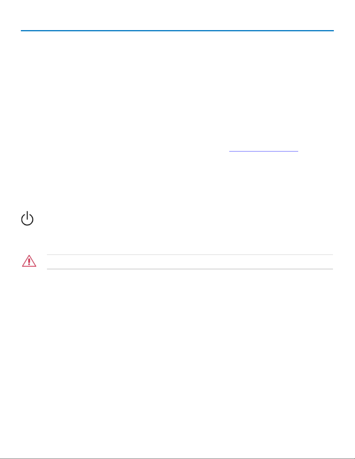
Powering On/Off

The Power button at the lower, left front of the oscilloscope controls the operational state of the instrument.

Press the button to switch on the instrument. The LED on the button lights to show the oscilloscope is operational.

CAUTION. Do not power on or calibrate the oscilloscope with a signal attached.

Press the button again to power down. You can also use the File > Shutdown menu option to execute a proper shut down process and preserve settings before powering down.

The Power button does not disconnect the oscilloscope from the AC power supply. The only way to fully power down the instrument is to unplug the AC power cord from the outlet.

We recommend unplugging the instrument if it will be unused for a long period of time.

WaveSurfer 3000 Oscilloscopes

Software Activation

The oscilloscope operating software (firmware and standard applications) is active upon delivery. At powerup, the oscilloscope loads the software automatically.

Firmware

Free firmware updates are available periodically from the Teledyne LeCroy website at:

teledynelecroy.com/support/softwaredownload.

Registered users can receive an email notification when a new update is released. Follow the instructions on the website to download and install the software.

Purchased Options

If you decide to purchase an option, you will receive a license key via email that activates the optional features on the oscilloscope. See Adding an Option Key for instructions on activating optional software packages.

Operator's Manual

Inputs/Outputs

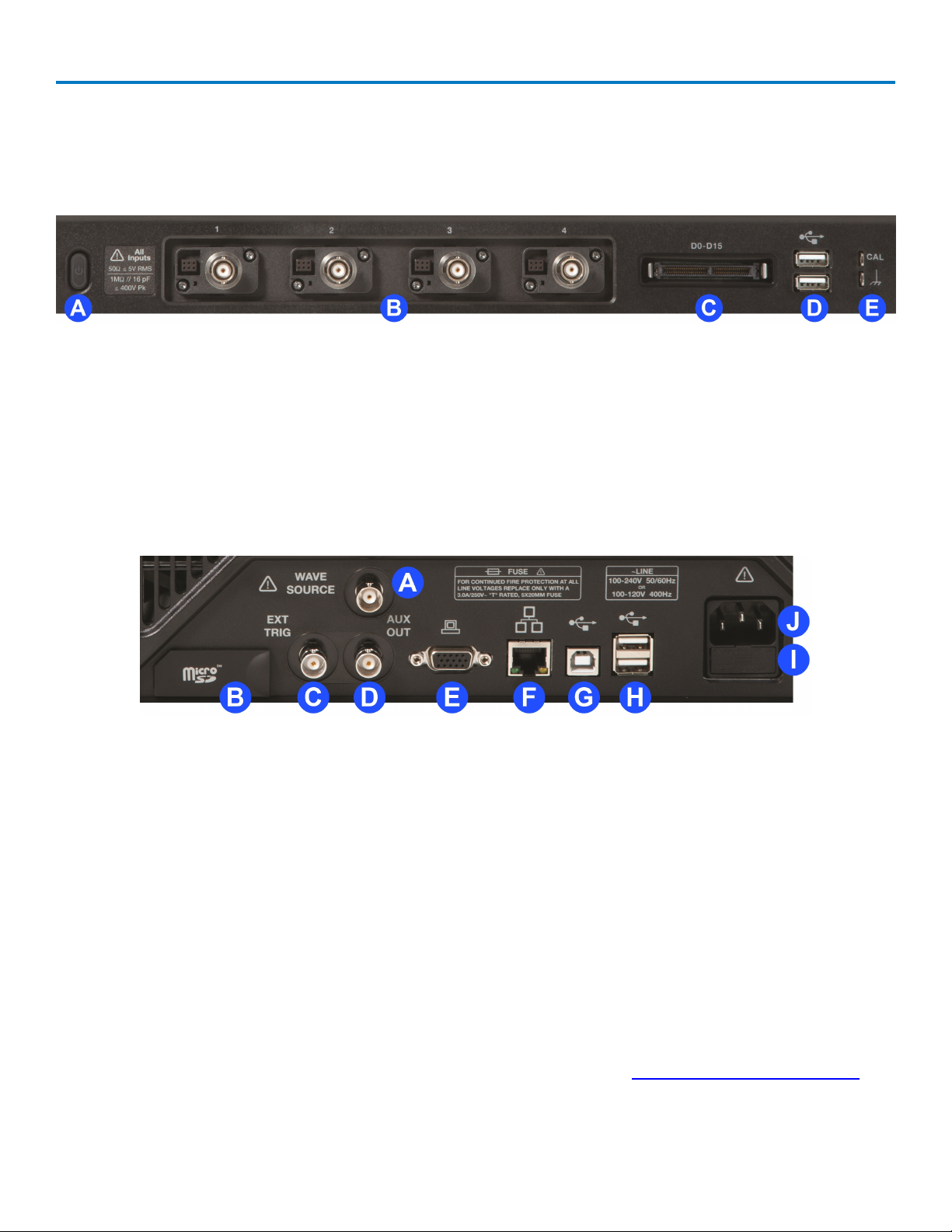
Front Input/Output Panel

A. Power button.

B. Channel inputs 1-4 for analog signals.

C. Front-mounted host USB ports for transferring data or connecting peripherals such as a mouse or

keyboard.

D. Ground and calibration output terminal used to compensate passive probes.

Back Input/Output Panel

A. WaveSource connector outputs signal generated by the internal waveform generator.

B. MicroSD Card slot.

C. EXT Trig connector accepts external trigger.

D. AUX OUT connector sends trigger out.

E. VGA connector sends video out to external monitors.

F. Ethernet port connects the oscilloscope to a LAN.

G. USBTMC port enables remote control of the oscilloscope.

H. Additional host USB ports (2) connect external devices such as printers or storage drives.

I. Fuse holder.

J. AC Power inlet.

See the general set up instructions for more information about configuring connections to other devices.

WaveSurfer 3000 Oscilloscopes

Analog Inputs

A series of BNC connectors arranged on the front of the oscilloscope are used to input analog signal on Channels 1-4. EXT, on the back of the oscilloscope, can be used to input an external trigger pulse.

Channel connectors use the ProBus interface. The ProBus interface contains a 6-pin power and communication connection and a BNC signal connection to the probe. It includes sense rings for detecting passive probes and accepts a BNC cable connected directly to it. ProBus offers 50 Ω and 1 MΩ input impedance and control for a wide range of probes.

The interfaces power probes and completely integrate the probe with the oscilloscope channel. Upon connection, the probe type is recognized and some setup information, such as input coupling and attenuation, is performed automatically. This information is displayed on the Probe Dialog, behind the Channel (Cx) dialog. System (probe plus oscilloscope) gain settings are automatically calculated and displayed based on the probe attenuation.

Probes

WaveSurfer3000 oscilloscopes are compatible with the included passive probes and all Teledyne LeCroy ProBus active probes that are rated for the oscilloscope’s bandwidth. Probe specifications and documentation are available at teledynelecroy.com/probes.

The passive probes supplied with your oscilloscope are matched to the input impedance of the instrument but may need further compensation. Follow the directions in the probe instruction manual to compensate the frequency response of the probes.

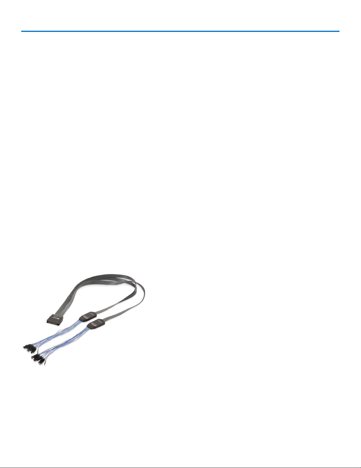
Digital Inputs

Available with the WS3K-MSO option, the digital leadset enables input of up-to-16 lines of digital data. Lines can be organized into two logical groups and renamed appropriately.

The digital leadset features two digital banks with separate Threshold controls, making it possible to simultaneously view data from different logic families.

Connecting/Disconnecting the Leadset

To connect the leadset to the oscilloscope, push the connector into the mixed signal interface below the front panel until you hear a click.

To remove the leadset, press in and hold the buttons on each side of the connector, then pull out to release it.

Operator's Manual

Grounding Leads

Each flying lead has a signal and a ground connection. A variety of ground extenders and flying ground leads are available for different probing needs.

To achieve optimal signal integrity, connect the ground at the tip of the flying lead for each input used in your measurements. Use either the provided ground extenders or ground flying leads to make the ground connection.

WaveSurfer 3000 Oscilloscopes

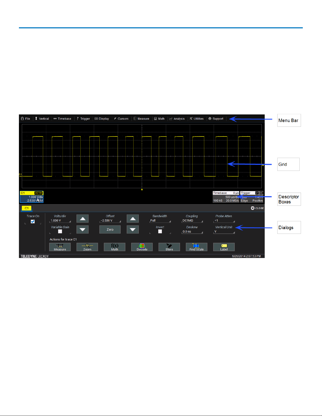
Touch Screen

The touch screen is the principal viewing and control center of the oscilloscope. The entire display area is active: use your finger or a stylus to touch, touch-and-drag, or draw a selection box. Many controls that display information also work as “buttons” to access other functions.

If you have a mouse installed, you can click anywhere you can touch to activate a control; in fact, you can alternate between clicking and touching, whichever is convenient for you.

The touch screen is divided into the following major control groups:

Menu Bar

The top of the window contains a complete menu of oscilloscope functions. Making a selection here changes the dialogs displayed at the bottom of the screen.

Many common oscilloscope operations can also be performed from the front panel or launched via the Descriptor Boxes. However, the menu bar is the best way to access dialogs for Save/Recall (File) functions, Display functions, Status, LabNotebook, and Utilities/Preferences setup.

Operator's Manual

Signal Display Grid

The grid area displays the waveform traces. It is sectioned into 10 Horizontal (Time) divisions and 8 Vertical (Voltage) divisions.

By default, the oscilloscope divides the screen into a maximum of three grids, one each for channels/memories, math functions, and zooms. All traces of the same type appear on the same grid.

Three other grid layouts are available: Single Grid, which displays all traces on the same grid, XY Grid, which puts the oscilloscope in XY mode, and XY Single Grid, which creates one XY grid and one single grid for the rest of your traces.

Different types of traces opening in separate grids.

Adjusting Grid Brightness

You can adjust the brightness of the grid lines to make either the grid or traces more visible. Go to Display > Display Setup and enter a new Grid Intensity percentage. The higher the number, the brighter and bolder the

grid lines.

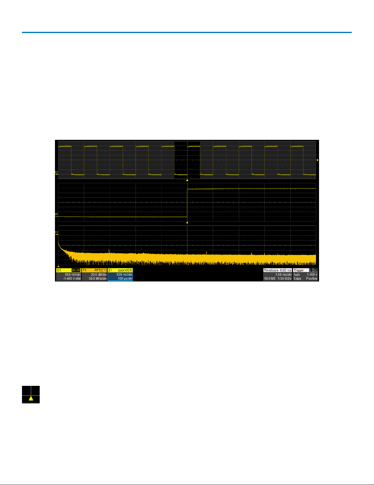
Grid Indicators

These indicators appear outside the grid to mark important points on the display. They are matched to the color of the trace to which they apply.

Trigger Position - A small triangle along the bottom (horizontal) edge of the grid shows the time the oscilloscope is set to trigger an acquisition. Unless Delay is set, this indicator is at the zero (center)

point of the grid. Trigger Delay is shown at the top right of the Timebase descriptor box.

WaveSurfer 3000 Oscilloscopes

Pre/Post-trigger Delay - A small arrow to the bottom left or right of the grid indicates that a pre- or post-trigger Delay has shifted the Trigger Position indicator to a point in time not displayed on the

grid. All trigger Delay values are shown on the Timebase Descriptor Box.

Trigger Level - This small triangle at the right edge of the grid tracks the trigger voltage level. If you

change the trigger level when in Stop trigger mode, or in Normal or Single mode without a valid trigger, a hollow triangle of the same color appears at the new trigger level. The trigger level indicator is not shown if the triggering channel is not displayed.

Zero Volts Level - This indicator is located at the left edge of the grid. One appears for each open

trace on the grid, sharing the number and color of the trace.

Various Cursor lines appear over the grid to indicate specific voltage and time values on the waveform. Touch-and-drag cursor indicators to quickly reposition them.

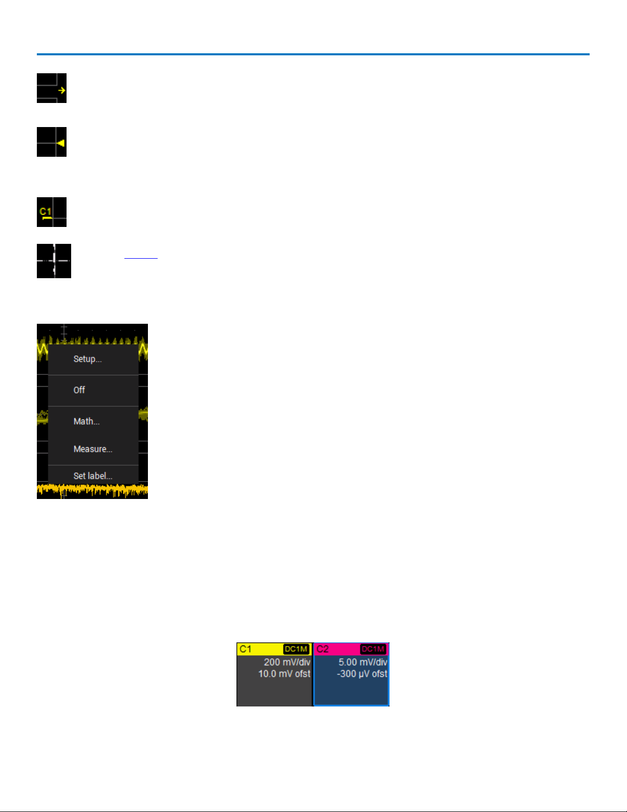
Grid Context Menu

Quickly touching a waveform trace opens a pop-up menu with shortcuts to the appropriate trace setup dialog, or the Math and Measure setup dialogs. You can also use it to turn off the trace or place an annotation label on it.

Descriptor Boxes

Shown just beneath the grid display, these boxes provide a summary of your channel, timebase and trigger settings. They also act as convenient navigation tools.

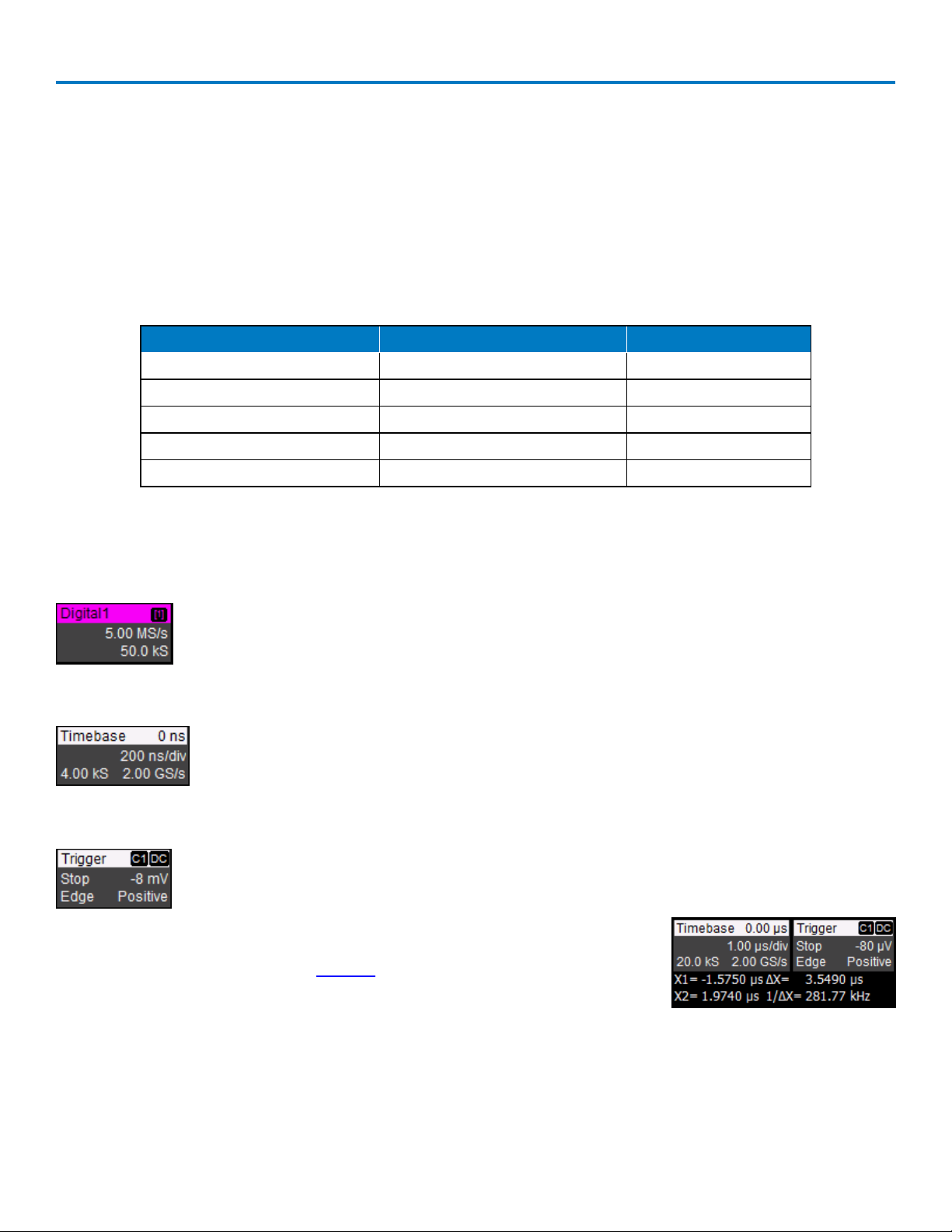
Descriptor boxes appear when a trace is turned on. Touch the descriptor box once to activate the trace. When a trace is active, its descriptor Box is highlighted, and front panel controls will work for that trace. Touch the descriptor box a second time to open its corresponding setup dialog.

Highlighted channel descriptor box (right) is active. Controls will work for this trace.

Operator's Manual

Channel Descriptor Box

Channel trace descriptor boxes correspond to analog signal inputs. They show Vertical settings and any Vertical cursor readouts: (clockwise from top left) Trace Number (Cx), Pre-Processing List (summarizes changes from default state), Coupling, Gain Setting, Offset Setting, and Averaging Sweeps Count.

Codes are used to indicate pre-processing that has been applied to the input. The codes have a long and short form. When several processes are in effect, the short form is used.

Preprocessing Symbols on Descriptor Boxes

Pre-Processing Type Long Form Short Form

Inversion INV I

Deskew DSQ DQ

Coupling DC50, DC1M or AC1M D50, D1M, or A1

Ground GND G

Bandwidth Limiting BWL B

Similar descriptor boxes appear for zoom (Zx), math (Fx), and memory (Mx) traces. These descriptor boxes show any Horizontal scaling that differs from the signal Timebase.

Digital Descriptor Box

Digital descriptor boxes (WS3K-MSO) appear whenever a digital line group is enabled. They are named Digital1 and Digital2 corresponding to one of the two line groups.They show the number of digital lines in the group, digital sample rate, and digital memory.

Timebase Descriptor Box

The TimeBase descriptor box shows: (clockwise from top right) Trigger Delay (position), Time/div, Sample Rate, Number of Samples, and Sampling Mode (blank when in real-time mode).

Trigger Descriptor Box

Trigger descriptor box shows: (clockwise from top right) Trigger Source and Coupling, Trigger Level (V), Slope, Trigger Type, Trigger Mode.

Setup information for Horizontal cursors, including the time between cursors and the frequency, is shown beneath the TimeBase and Trigger descriptor boxes. See the Cursors section for more information.

WaveSurfer 3000 Oscilloscopes

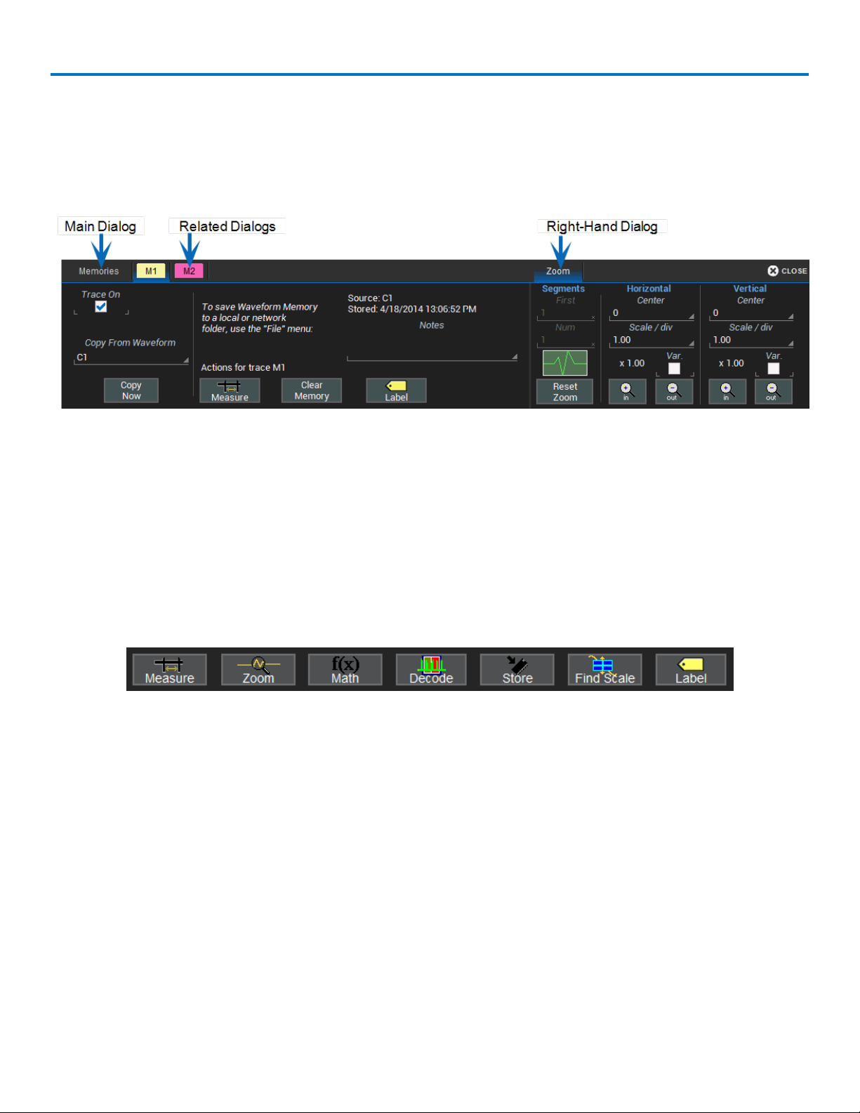
Dialogs

Dialogs appear at the bottom of the display for entering setup data. The top dialog will be the main entry point for the selected setup option. For convenience, related dialogs appear as a series of tabs behind the main dialog. Touch the tab to open the dialog.

Right-Hand Dialogs

At times, your selections will require more settings than normally appear (or can fit) on a dialog, or the task commonly invites further action, such as zooming a new trace. In that case, sub-dialogs will appear to the right-side of the main dialog. These right-hand dialog settings always apply to the object that is being configured on the left-hand dialog.

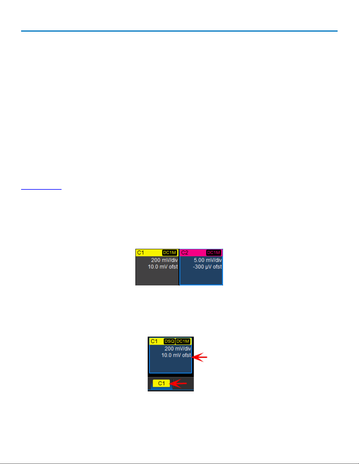
Action Toolbar

Several setup dialogs contain a toolbar at the bottom of the dialog. These buttons apply common actions without having to leave the underlying set up dialog. They always apply to the active trace.

Measure opens the Measure pop-up to set measurement parameters on the active trace.

Zoom creates a zoom trace of the active trace.

Math opens the Math pop-up to apply math functions to the active trace and create a new math trace.

Decode opens the main Serial Decode dialog where serial data decoders can be configured and applied. This

button is only active if you have decoder software options installed.

Store loads the active trace into the corresponding memory location (C1, F1 and Z1 to M1; C2, F2 and Z2 to M2, etc.).

Find Scale automatically performs a vertical scaling that fits the waveform into the grid.

Label opens the Label pop-up to annotate the active trace.

Operator's Manual

Turning On/Off Traces

Analog Trace

From the display, choose Vertical > Channel <#> Setup to turn on the trace. To turn it off, clear the Trace On checkbox on the corresponding Channel dialog.

From the front panel, press the Channel button (1-4) to turn on the trace; press again to turn it off.

Digital Trace

From the display, choose Vertical > Digital <#> Setup.

From the front panel, press the Dig button, then check Group on the Digital<#> trace dialog. Clear Group to turn off the trace.

Other Traces

You can quickly create zoom or math traces without leaving the setup dialogs by touching the Zoom or Math

toolbar button at the bottom of the dialog. Also use the front panel Zoom, Math, or Mem(ory) buttons to

quickly create traces.

Activating Traces

A trace descriptor box appears on the display for each enabled trace. Touch this box at any time to activate the trace; touch it again to open the setup dialog. A highlighted descriptor box indicates the active trace to which all actions apply.

Inactive trace descriptor (left), active trace descriptor (right).

Although several traces may be open and appear on the grid, only one at a time is active. When you activate a trace, the dialog at the bottom of the screen automatically switches to the appropriate setup dialog for that trace. The tab at the top of the dialog shows to which trace it applies.

Active descriptor label matches active setup dialog tab.

WaveSurfer 3000 Oscilloscopes

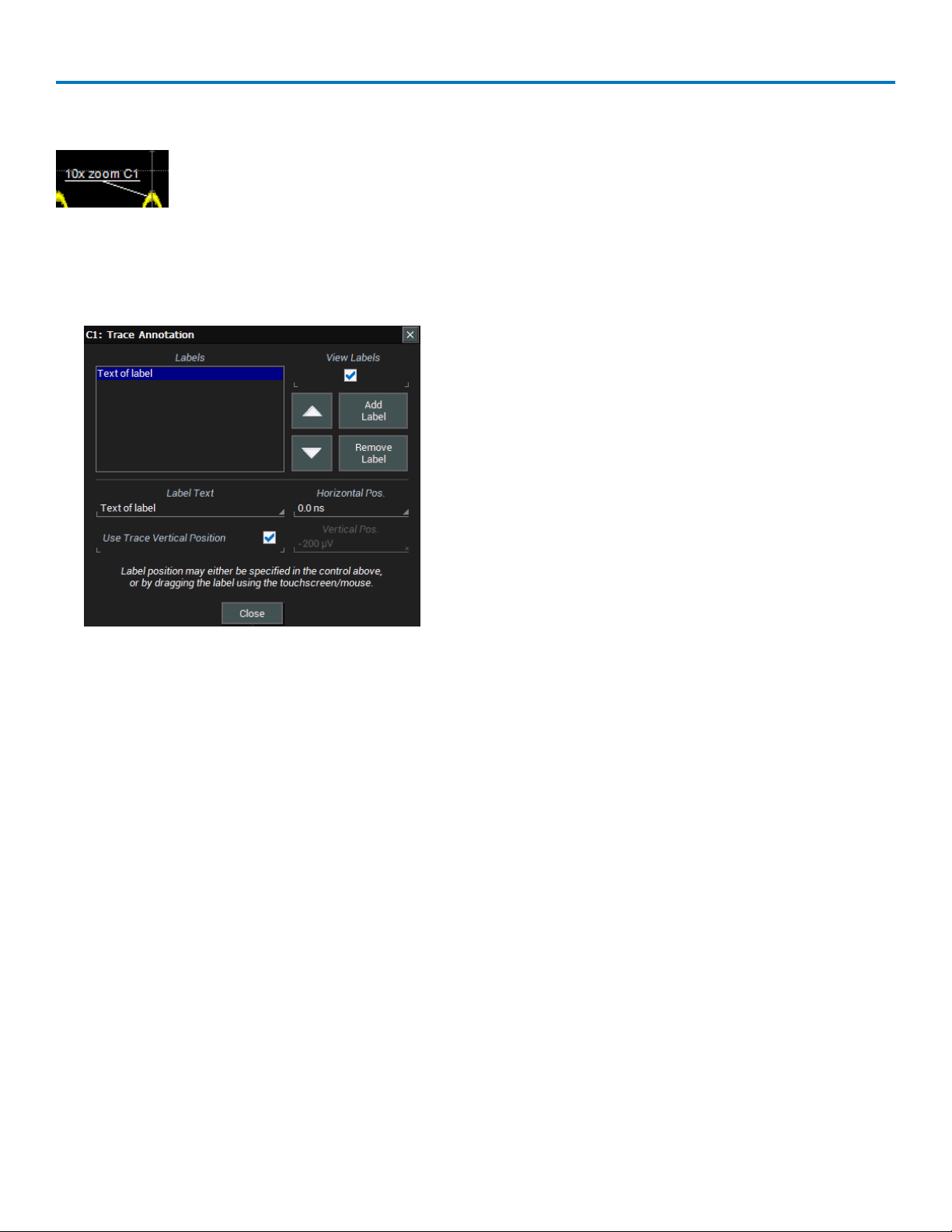
Annotating Traces

The Label function gives you the ability to add custom annotations to traces that are shown on the display. Labels are numbered sequentially in the order they were created. Once placed, labels can be moved to new positions or turned off.

Create Label

1. Touch the trace and choose Set label... from the context menu, or touch the trace descriptor box twice and touch the Label toolbar button on the setup dialog.

2. On the Trace Annotation pop-up, touch Add Label.

3. Enter the Label Text.

4. Optionally, enter the Horizontal Pos. and Vertical Pos. (in same units as the trace) at which to place the label. The default position is 0 ns horizontal. You can optionally check Use Trace Vertical Position instead of entering a Vertical Pos.

Reposition Label

Once placed, drag-and-drop labels to a new position on the grid, or reopen the Trace Annotation pop-up and enter a new Horizontal Pos. and Vertical Pos.

Edit/Remove Label

Open the Trace Annotation pop-up and select the Label. You can use the Up/Down arrow keys to scroll the list. Change the Label Text or Horizontal and Vertical Pos.(itions). Touch Remove Label to delete it.

Turn On/Off Labels

After labels have been placed, you can turn on/off all labels at once by opening the Trace Annotation dialog and selecting/deselecting the View labels checkbox.

Entering/Selecting Data

Touch

Touch once to activate a control. In some cases, you’ll immediately see a pop-up menu of options. Touch one to select it.

TIP: You can touch the Icon or List buttons where they appear on larger pop-ups to change how menu options are displayed.

In other cases, data entry fields appear highlighted in blue when you touch them. When a data entry field is highlighted, it is active and can be modified by using the front panel Adjust knob. Or, touch it again and use the pop-up menu or keypad to make an entry.

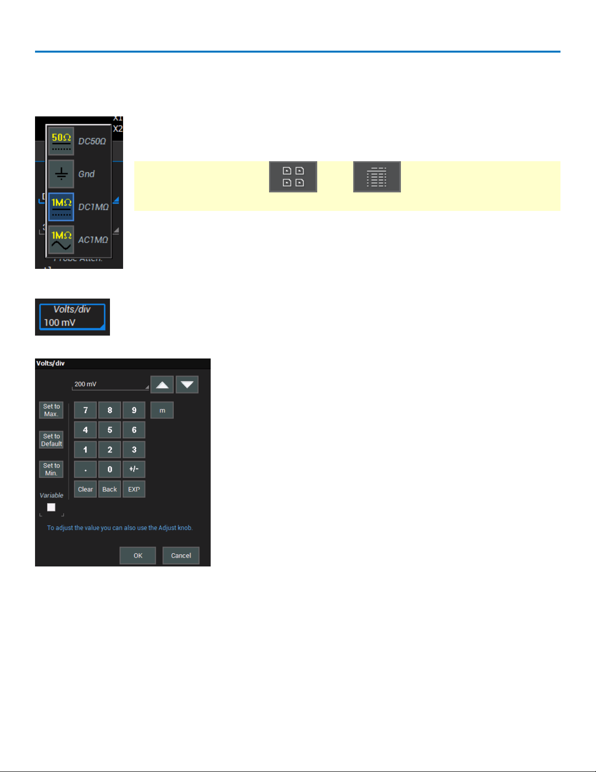
Operator's Manual

You’ll see a pop-up keypad when you touch twice on a numerical data entry field. Use it exactly as you would a calculator. When you touch OK, the calculated value is entered in the field.

The Set to... buttons quickly enter the maximum, default or minimum value for that field.

The Up and Down arrow buttons increment/decrement the displayed value.

The Variable checkbox allows you to make fine increment changes when using the Up and Down arrow buttons.

WaveSurfer 3000 Oscilloscopes

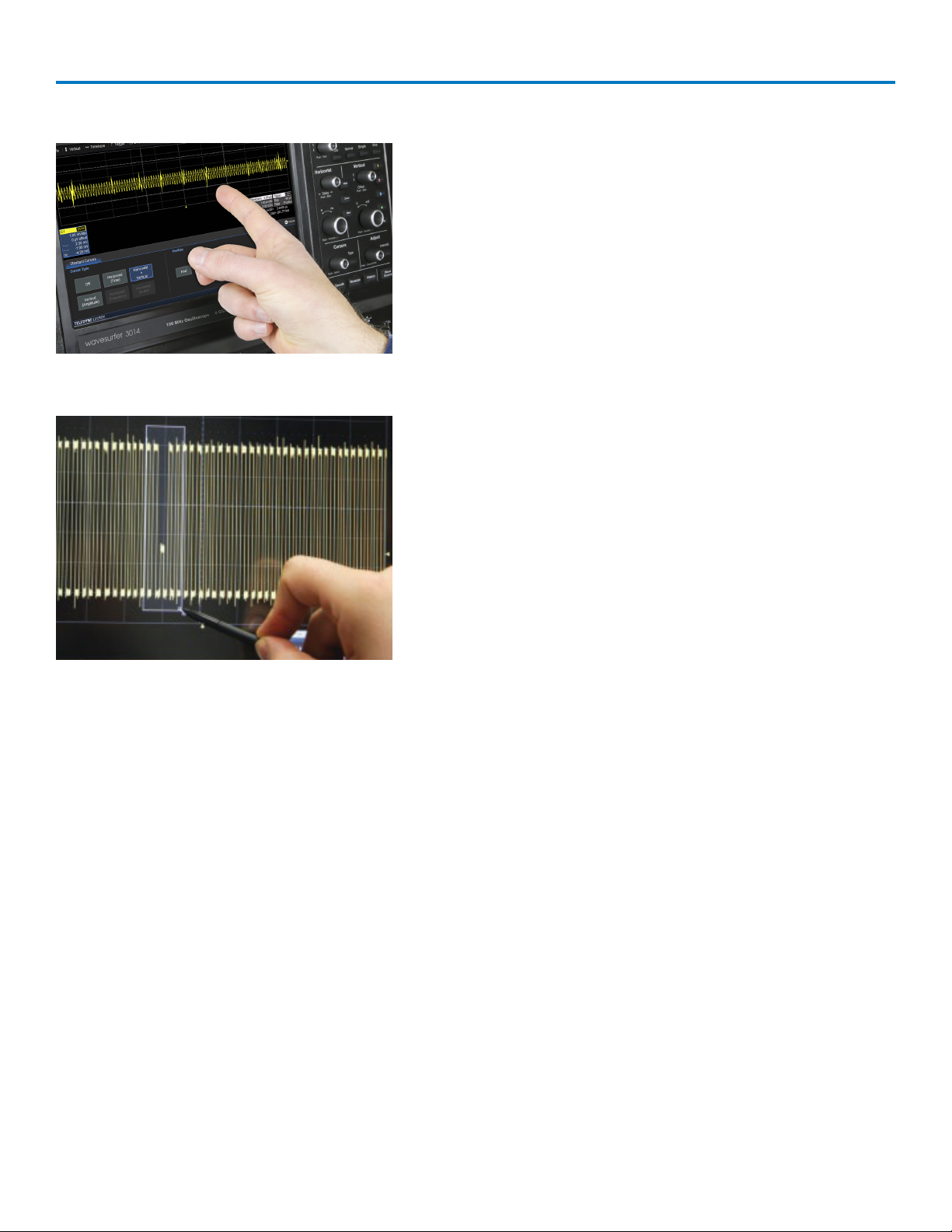
Touch & Drag

Touch-and-drag cursor lines and annotation labels to reposition them on the grid; this is the same as setting the values on the dialog.

Touch-and-drag to draw a selection box around part of a trace to quickly zoom that portion.

Operator's Manual

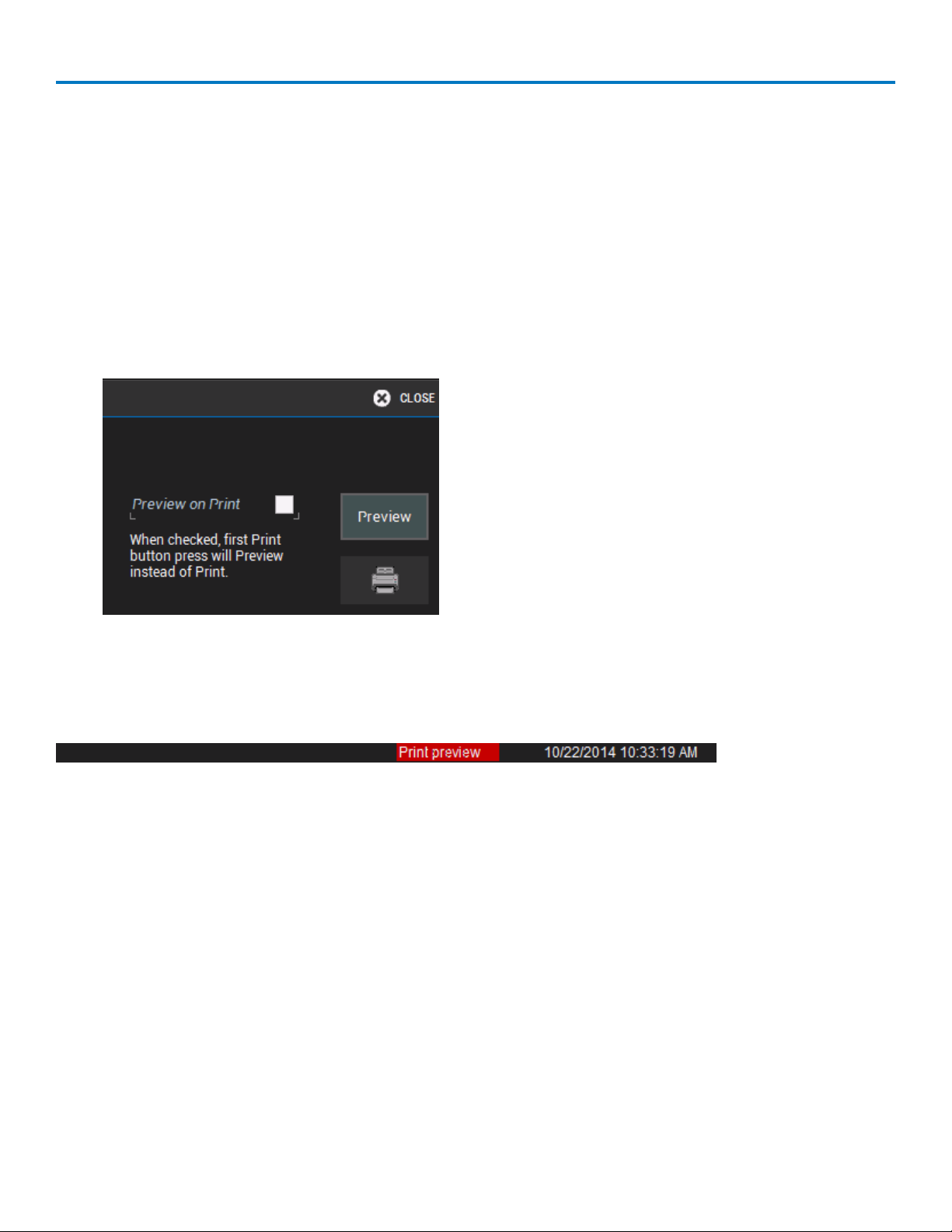
Print Preview

The Print Preview feature allows you to pause the fast display for closer waveform inspection or printing. No function other than printing is available when in Print Preview mode. All oscilloscope analysis functions (such as measurement calculations) are also paused.

There are three ways to invoke Print Preview:

l On the Utilities > Utilities Setup > Hardcopy dialog, check the box labeled Preview on Print. This

configures the front panel Print button button so that the first press puts the oscilloscope into Print Preview mode, and the second press prints the screen image according to the Hardcopy setup.

l On the Utilities > Utilities Setup > Hardcopy dialog, touch the Preview button above the Print button.

l From the menu bar, choose File > Print Preview. A green checkmark appears next to the menu option

to show you are in Preview mode.

Following any of these actions, you should see the message "Print preview" appear in red at the right of the message bar.

When you go on to print the screen, you will see the message "Hardcopy saved to..." (or "Printing started..." if sending to a printer) at the left of the message bar.

Operating any other dialog or front panel control ends the Print Preview and resumes acquisition processing.

WaveSurfer 3000 Oscilloscopes

Printing/Screen Capture

The Print function captures an image of the display and outputs it according to your Hardcopy settings.

There are three ways to print a capture of the screen:

l Touch the front panel Print button.

l Choose File > Print.

l Choose Utilities > Utilities Setup > Hardcopy tab and touch the Print button to the far right of the

dialog.

NOTE: When the front panel Print button is configured to capture the screen as a LabNotebook entry, only the File and Utilities menu print options will function according to your Hardcopy setup.

Language Selection

To change the language that appears on the touch screen:

1. Go to Utilities > Preference Setup > Preferences and make your Language selection.

2. Follow the prompt to restart the oscilloscope application.

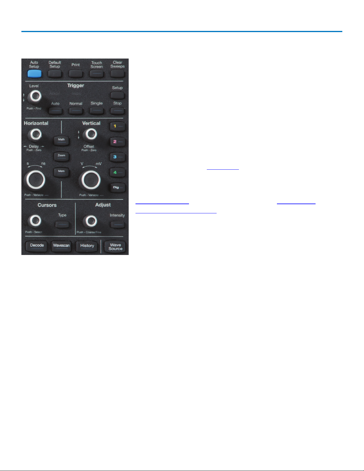
Front Panel

Operator's Manual

Most front panel controls duplicate functionality available through the touch screen display and are described on the following pages.

All the knobs on the front panel function one way if turned and another if pushed like a button. The top label describes the knob’s “turn” action, the bottom label its “push” action.

Front panel buttons light up to indicate which traces and functions are active. Actions performed from the front panel always apply to the active trace.

Top Row Buttons

Auto Setup performs an Auto Setup.

Default Setup resets the oscilloscope to the factory defaults.

Print captures the entire screen and outputs it according to your

Hardcopy settings. It can also be configured for Print Preview or to output a LabNotebook entry.

Touch Screen enables/disables touch screen functionalilty.

Clear Sweeps resets the acquisition counter and any cumulative

measurements.

Trigger Controls

Level knob changes the trigger threshold level (V). The number is shown on the Trigger descriptor box. Pushing the knob sets the trigger level to the 50% point of the input signal.

READY indicator lights when the trigger is armed. TRIG'D is lit momentarily when a trigger occurs. A fast trigger rate causes the light to stay lit continuously.

Setup corresponds to the menu selection Trigger > Trigger Setup. Press it once to open the Trigger Setup dialog and again to close the dialog.

Auto turns on Auto trigger mode. The oscilloscope triggers after a time-out, even if the trigger conditions are not met.

Normal turns on Normal trigger mode. The oscilloscope triggers each time a signal is present that meets the conditions set for the type of trigger selected.

Single turns on Single trigger mode. The oscilloscope triggers once (single-shot acquisition) when the input signal meets the trigger conditions. If the scope is already armed, it will force a trigger.

Stop prevents the oscilloscope from triggering on a signal. If you boot up the instrument with the trigger in Stop mode, a "No trace available" message is shown. Press the Auto button to display a trace.

WaveSurfer 3000 Oscilloscopes

Horizontal Controls

The Delay knob changes the Trigger Delay value (S) when turned. Push the knob to reset Delay to zero.

The Horizontal Adjust knob sets the Time/division (S) of the oscilloscope acquisition system when the trace source is an input channel. The Time/div value is shown on the Timebase descriptor box. When using this control, the oscilloscope allocates memory as needed to maintain the highest sample rate possible for the timebase setting. When the trace is a zoom, memory or math function, turn the knob to change the horizontal scale of the trace, effectively "zooming" in or out. By default, the knob adjusts values in 1, 2, 5, 10 step increments. Push the knob to change the action to fine increments; push it again to return to stepped increments.

Vertical Controls

Channel buttons turn on a channel that is off, or activate a channel that is already on. When the channel is active, pushing its channel button turns it off. A lit button shows the active channel.

Offset knob adjusts the zero level of the trace (this makes it appear to move up or down relative to the center axis of the grid). The value appears on the trace descriptor box. Push it to reset Offset to zero.

Gain knob sets Vertical Gain (V/div). The value appears on the trace descriptor box. By default, the knob adjusts values in 1, 2, 5, 10 step increments. Push the knob to change the action to fine increments; push it again to return to stepped increments.

Dig button enables digital input through the Digital Leadset on -MS models.

Math, Zoom, and Mem(ory) Buttons

The Zoom button creates a quick zoom for each open channel trace. Touch the zoom trace descriptor box to display the zoom controls.

The Math and Mem(ory) buttons open the corresponding setup dialogs.

If a Zoom, Math or Memory trace is active, the button illuminates to indicate that the Vertical and Horizontal knobs will now control that trace.

Cursor Controls

Cursors identify specific voltage and time values on the waveform. The white cursor lines help make these points more visible. A readout of the values appears on the trace descriptor box.

There are five preset cursor types, each with a unique appearance on the display. These are described in more detail in the Cursors section.

Type selects the cursor type. Continue pressing to cycle through all cursor until the desired type is found. The type "Off" turns off the cursor display.

Cursor knob repositions the selected cursor line when turned. Push to select a different cursor line to adjust.

Operator's Manual

Adjust and Intensity Controls

The Adjust knob changes the value in any highlighted data entry field when turned. Pushing the Adjust knob toggles between coarse (large increment) or fine (small increment) adjustments when the knob is turned.

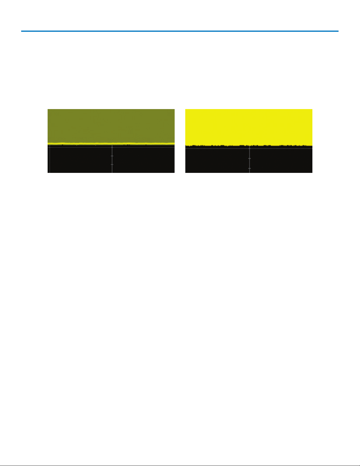
When more data is available than can actually be displayed, the Intensity button helps to visualize significant events by applying an algorithm that dims less frequently occurring samples. This feature can also be accessed from the Display Setup dialog.

Intensity 40% (left) dims samples that occur ≤ 40% of the time to highlight the more frequent samples, vs. intensity 100% (right)

which shows all samples at the same intensity.

Bottom Row Buttons

Decode opens the Serial Decode dialog if you have serial data decoder options installed.

WaveScan opens the WaveScan dialog.

History opens the History Mode dialog.

WaveSource opens the WaveSource internal waveform generator dialog if you have the function generator

option installed.

WaveSurfer 3000 Oscilloscopes

Zooming Waveforms

The Zoom function magnifies a selected region of a trace. On WaveSurfer 3000 model oscilloscopes, you can display up to four zoom traces (Z1-Z4) taken from any channel, math, or memory trace.

Creating Zooms

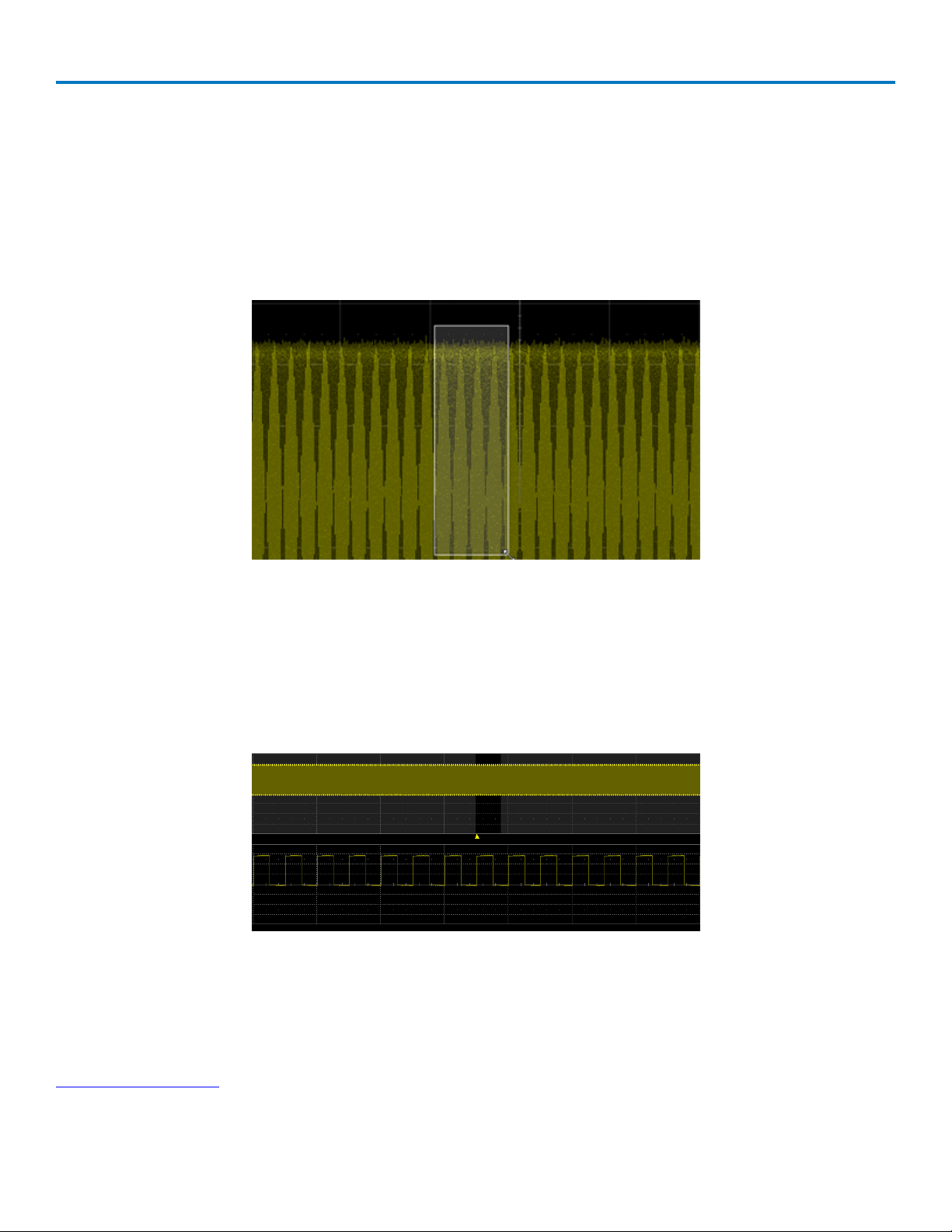
To create a zoom, touch -and-drag to draw a selection box around any part of the source waveform.

Selection box over trace.

The zoom will resize the selected portion to fit the full width of the grid. The degree of vertical and horizontal magnification, therefore, depends on the size of the rectangle that you draw.

The zoom opens in a new grid, with the area around the zommed portion shaded. New zooms are turned on and visible by default. However, you can turn off a particular zoom if the display becomes too crowded, and the zoom settings are saved in its Zx location, ready to be turned on again when desired.

Area around zoomed portio shaded.

Adjust Zoom

The zoom's Horizontal units will differ from the signal timebase because the zoom is showing a calculated scale, not a measured level. This allows you to adjust the zoom factor using the front panel knobs or the

Zoom dialog controls however you like without affecting the timebase (a characteristic shared with math

Operator's Manual

and memory traces).

Turn off Zoom

To close the zoom, either touch the zoom descriptor box twice to open the Zoom dialog and deselect Trace On, or touch the zoom trace to open the context menu and choose Off.

Zoom Controls

To open the Zoom dialog, touch twice on any zoom descriptor box, or choose Math > Zoom Setup from the menu bar.

Trace Controls

Trace On shows/hides the zoom trace. It is selected by default when the zoom is created.

Source lets you change the source for this zoom to any channel, math, or memory trace while maintaining all

other settings.

Segment Controls

These controls are used in Sequence Sampling Mode.

Zoom Factor Controls

These controls on the Zx dialogs appear throughout the oscilloscope software:

l Out and In buttons increase or decrease the magnification of the zoom, and consequently change the

Horizontal andVertical Scale settings. Continue to touch either button until you've achieved the desired level of zoom.

l Horizontal Scale/div sets the amount of time represented by each horizontal division of the grid. It is

the equivalent of Time/div, only unlike the Timebase setting, it may be set differently for each zoom, math function, or memory trace.

l Horizontal Center sets the voltage or time that is to be at the center of the screen on the zoom trace.

The horizontal center is the same for all zoom traces.

l Reset Zoom returns the zoom to x1 magnification.

WaveSurfer 3000 Oscilloscopes

Vertical

Vertical, also called Channel, settings usually relate to voltage level and control the trace along the Y axis.

NOTE:While Digital settings can be accessed through the Vertical menu on oscilloscopes with the Mixed Signal option, they are handled quite differently. See Digital.

The amount of voltage displayed by one vertical division of the grid, or Vertical Scale (V/div), is most quickly adjusted by using the front panel Vertical knob. The Channel descriptor box always shows the current Vertical Scale setting.

If a Teledyne LeCroy probe is connected to the channel, a Probe dialog appears behind the Cx dialog.

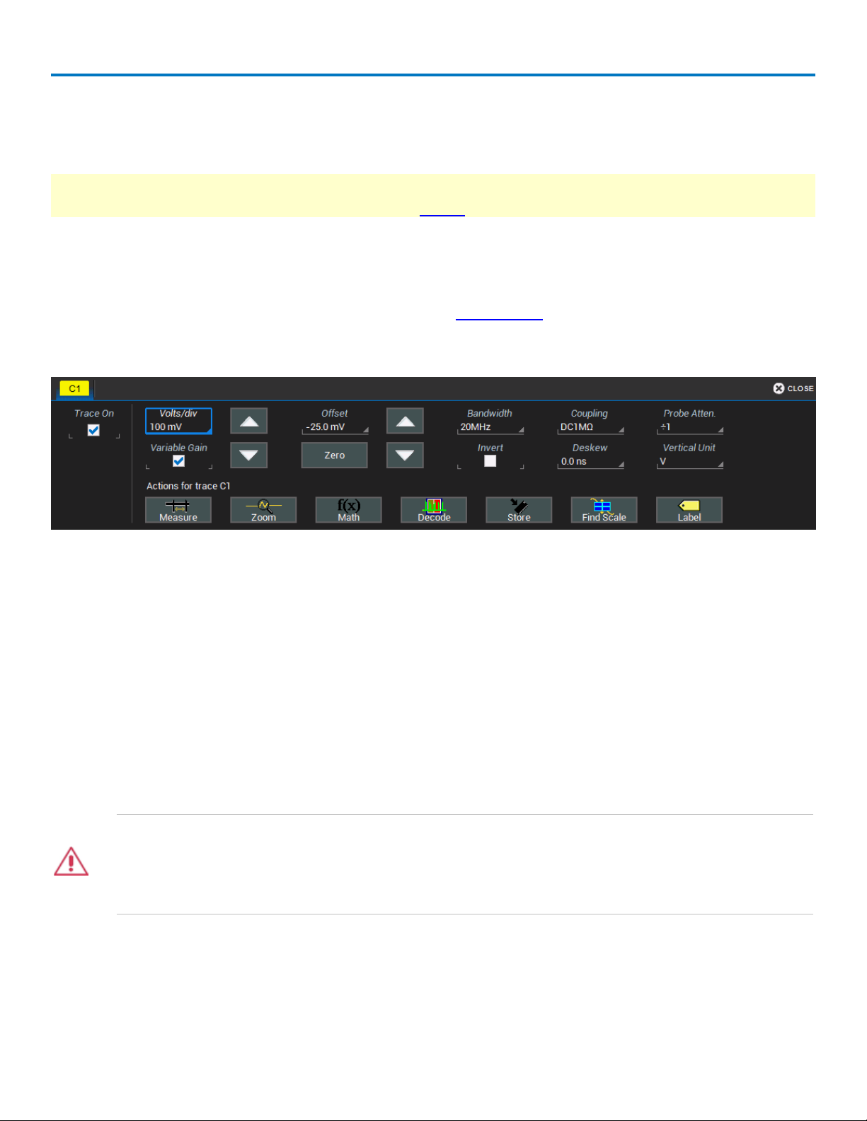
Channel Settings

Volts/div sets the vertical scale (aka gain or sensitivity). Select Variable Gain adjustment or leave the checkbox clear for fixed adjustment.

Offset adds a defined value of DC offset to the signal as acquired by the input channel. This may helpful in order to display a signal on the oscilloscope grid while maximizing the vertical height (or gain) of the signal. A negative value of offset will "subtract" a DC voltage value from the acquired signal (and move the trace down on the grid") whereas a positive value will do the opposite. Touch Zero Offset to return to zero.

A variety of Bandwidth filters are available at a variety of fixed settings. The exact settings vary by model. To limit bandwidth, select a filter from this field.

Invert inverts the waveform for the selected channel.

Coupling may be set to DC 50 Ω, DC1M, AC1M or GROUND (Gnd).

CAUTION. The maximum input voltage depends on the input used. Limits are displayed on the front

of the oscilloscope. Whenever the voltage exceeds this limit, the coupling mode automatically switches to GROUND. You then have to manually reset the coupling to its previous state. While the unit does provide this protection, damage can still occur if extreme voltages are applied.

Deskew adjusts the amount of horizontal time offset to compensate for propagation delays caused by different probes or cable lengths. The valid range depends on the current timebase setting. The Math deskew function performs the same activity.

Operator's Manual

Probe Settings

When a Teledyne LeCroy-compatible probe is connected to the oscilloscope input, the probe is automatically identified and the model name displayed on the Channel dialog under the "Probe" heading. Also, the Probe dialog bearing the probe name is added to the right of the Channel dialog. When a probe is not connected, the Channel dialog shows only the Cx tab for vertical setup.

When third-party probes are connected, an Attenuation field appears on the Cx dialog, with a default value of /1, allowing you to enter attenuation and rescale values manually.

Channel dialog with tab for connected probe.

The Probe Dialog displays probe attributes and (depending on the probe type) allows you to AutoZero or DeGauss probes from the oscilloscope touch screen. Other settings may appear, as well, depending on the probe model.

Probe dialog showing the connected probe's control attributes.

Auto Zero Probe

Auto Zero corrects for DC offset drifts that naturally occur from thermal effects in the amplifier of active probes. Teledyne LeCroy probes incorporate Auto Zero capability to remove the DC offset from the probe's amplifier output to improve the measurement accuracy.

CAUTION. Remove the probe from the circuit under test before initializing AutoZero.

WaveSurfer 3000 Oscilloscopes

DeGauss Probe

The Degauss control is activated for some types of probes (e.g., current probes). Degaussing eliminates residual magnetization from the probe core caused by external magnetic fields or by excessive input. It is recommended to always degauss probes prior to taking a measurement.

CAUTION. Remove the probe from the circuit under test before initializing DeGauss.

Auto Setup

Auto Setup quickly configures the essential oscilloscope settings based on the first input signal it finds, starting with Channel 1. If nothing is connected to Channel 1, it searches Channel 2 and so forth until it finds a signal. Vertical Scale (V/div), Offset, Timebase (Time/div), and Trigger are set to an Edge trigger on the first, non-zero-level amplitude, with the entire waveform visible for at least 10 cycles over 10 horizontal divisions.

To run Auto Setup, press the front panel Auto Setup button.

Restore Default Setup

Restore the oscilloscope to its factory default state by pressing the front panel Default Setup button. You can also restore default settings by choosing File > Recall Setup > Recall Default.

Default settings for your oscilloscope include the following:

Channel/Vertical C1-C4 on at 50 mV/div Scale, 0 V Offset

Timebase Real Time Sampling at 50 ns/div, 0 Delay, 2.0 kS at 4 GS/s, 100 kS Memory

Trigger C1 with an Auto Positive Edge, DC Coupling, 0 V Level

Display Auto Grid

Cursors Off

Measurements Cleared

Math Cleared

Operator's Manual

Viewing Status

All oscilloscope settings can be viewed through the various Status dialogs. These show all existing acquisition, trigger, channel, math function, measurement and parameter configurations, as well as which are currently active.

Access the Status dialogs by choosing the Status option from the Vertical, Timebase, Trigger, or Math menus (e.g., Channel Status, Acquisition Status).

WaveSurfer 3000 Oscilloscopes

Digital (Mixed Signal)

The digital leadset (delivered with the WS3K-MSO option) inputs up-to-16 lines of digital data. Leads are organized into two banks of eight leads each, and you assign each bank a standard Logic Family or a custom Threshold to define the digital logic of the signal.

The Digital set up dialog has two tabs each corresponding to one of two possible digital groups, labeled Digital1 to Digital2, which correspond to buses. You choose which lines from among the 16 make up each digital group, what they are named, and how the group appears on the display. Initially, logical lines are numbered the same as the physical lead they represent, although any line number can be re-assigned to any lead.

Digital Traces

When a digital group is enabled, digital Line traces show which lines are high, low, or transitioning relative to the threshold. You can also view a digital Bus trace that collapses all the lines in a group into their Hex values.

Group of four traces displayed with a Vertical Position of positive 4.0 (top of grid) and a Group Height 4.0 (half the grid).

Digital Group Set Up

1. From the menu bar, choose Vertical > Digital <#> Setup, or press the front panel Dig button and select the desired Digital<#> tab.

Operator's Manual

2. On the Digital<#> set up dialog, check the boxes for lines D0 through D15 that comprise the group.

Touch the Display D0-D7 and Display D8-D15 buttons to quickly turn on the entire digital bank, or touch the Right and Left Arrow buttons to switch between each digital bank as you make line selections.

NOTE: Each group can consist of anywhere from 1 to 16 of the leads that are (or will be) connected to signal, from either digital bank regardless of the Logic set on the bank. It does not matter if the some or all of the lines have been included in other groups.

3. When all group members are selected, optionally rename them.

4. Go on to set up the digital display for the group. Check Group to enable the display.

5. When you're finished on the Digital<#> dialog, touch the Logic Setup tab and choose the Logic Family that applies to each digital bank, or set custom Threshhold values.

Digital Display Set Up

You can choose the type and position of the digital traces that appear on screen for each digital group.

1. Set up the digital group.

2. Choose a Display Mode:

l Lines (default) shows a time-correlated trace indicating high, low, and transitioning points (relative

to the Threshold) for every digital line in the group. The size and placement of the lines depend on the number of lines, the Vertical Position and Group Height settings.

l Bus collapses the lines in a group into their Hex values. It appears immediately below all the Line

traces when both are selected.

l Lines & Bus displays both line and bus traces at once.

3. In Vertical Position, enter the number of divisions (positive or negative) relative to the zero line of the grid where the display begins.The top of the first trace appears at this position.

4. In Group Height, enter the total number of grid divisions the entire display should occupy. All the selected traces (Line and Bus) will appear in this much space.

WaveSurfer 3000 Oscilloscopes

Individual traces are resized to fit the total number of divisions available. The example above shows a group of three Line traces plus the Bus trace occupying a Group Height of 4.0 divisions. Each trace takes up one division.

5. Check the Group box to enable the display.

To close traces, uncheck the Group box.

Renaming Digital Lines

The labels used to name each line can be changed to make the user interface more intuitive. Also, labels can be "swapped" between lines.

Changing Labels

1. Set up the digital group.

2. Touch Label and select from:

l Data - the default, which appends "D." to the front of each line number.

l Address - appends "A." to the front of each line number.

l Custom - lets you create your own labels line by line.

3. If using Custom labels:

l Touch the Line number button below the corresponding checkbox. If necessary, use the Left/Right

Arrow buttons to switch between banks.

l Use the virtual keyboard to enter the name, then press OK.

The button and any active line traces are renamed accordingly.

Swapping Lines

This procedure helps in cases where the physical lead number is different from the logical line number you would like to assign to that input (e.g., a group is set up for lines 0-4, but lead 5 was accidentally attached to the probing point). It can save time having to re-attach leads or re-configure groups.

1. Select a Label of Data or Address.

2. Touch the Line number button below the corresponding checkbox. If necessary, use the Left/Right Arrow buttons to switch between banks.

3. From the popup, choose the line with which you want to swap labels.

The button and any active line traces are renumbered accordingly.

Operator's Manual

Timebase

Timebase, also known as Horizontal, settings control the trace along the X axis. The timebase is shared by all channels.

The time represented by each horizontal division of the grid, or Time/Division, is most easily adjusted using the front panel Horizontal knob. Full Timebase set up, including sampling mode selection, is done on the Timebase dialog, which can be accessed by either choosing Timebase > Horizontal Setup from the menu bar, or touching the Timebase descriptor box.

The Timebase dialog contains settings for Sampling Mode, Timebase Mode, Real Time Memory.

Timebase Settings

Sampling Mode

Choose from Real Time, Sequence, RIS, Roll, or Average mode.

Timebase Mode

Time/Division is the time represented by one horizontal division of the grid. Touch the Up/Down Arrow buttons on the Timebase dialog or turn the front panel Horizontal knob to adjust this value.

Delay is the amount of time relative to the trigger event to display on the grid. In Real Time sampling mode, the trigger event is placed at time zero on the grid. Delay may be time pre-trigger, entered as a negative value, or post-trigger, entered as a positive value. Raising/lowering the Delay value has the effect of shifting the trace to the right/left, enabling you to focus on the relevant portion of longer acquisitions.

Set to Zero returns Delay to zero.

Real Time Memory

Maximum Points is the maximum number of samples taken per acquisition. The actual number of samples acquired can be lower due to the current Sample Rate and Time/Division settings.

WaveSurfer 3000 Oscilloscopes

Sampling Modes

Real Time Sampling Mode

Real Time sampling mode is a series of digitized voltage values sampled on the input signal at a uniform rate. These samples are displayed as a series of measured data values associated with a single trigger event. By default, the waveform is horizontally positioned so that the trigger event is time zero on the grid.

The relationship between sample rate, memory, and time can be expressed as:

Capture Interval = 1/Sample Rate X Memory

Capture Interval/10 = Time Per Division

In Real Time sampling mode, the acquisition can be displayed for a specific period of time (or number of samples) either before or after the trigger event occurs, known as trigger delay. This allows you to isolate and display a time/event of interest that occurs before or after the trigger event.

l Pre-trigger delay displays the time prior to the trigger event. This can be set from a time well before

the trigger event to the moment the event occurs, up to the oscilloscope's maximum sample record length. How much actual time this represents depends on your timebase setting. When set to the maximum allowed pre-trigger delay, the trigger position (and zero point) is off the grid (indicated by the trigger delay arrow at the lower right corner), and everything you see represents pre-trigger time.

l Post-trigger delay displays time following the trigger event. Post-trigger delay can cover a much

greater lapse of time than pre-trigger delay, up to the equivalent of 10,000 time divisions after the trigger event occurred. When set to the maximum allowed post-trigger delay, the trigger point may actually be off the grid far to the left of the time displayed.

Usually, on fast timebase settings, the maximum sample rate is used when in Real Time mode. For slower timebase settings, the sample rate is decreased so that the maximum number of data samples is maintained over time.

Sequence Sampling Mode

In Sequence Mode, the complete waveform consists of a number of fixed-size segments (see the instrument specifications at teledynelecroy.com for the limits). The oscilloscope uses the sequence timebase setting to determine the capture duration of each segment as 10 x time/div. With this setting, the oscilloscope uses the desired number of segments, maximum segment length, and total available memory to determine the actual number of samples or segments, and time or points.

Sequence Mode is ideal when capturing many fast pulses in quick succession or when capturing few events separated by long time periods. The instrument can capture complicated sequences of events over large time intervals in fine detail, while ignoring the uninteresting periods between the events. You can also make time measurements between events on selected segments using the full precision of the acquisition timebase.

Operator's Manual

SET UP SEQUENCE MODE

When setting up Sequence Mode, you define the number of fixed-size segments acquired in single-shot mode (see the instrument specifications for the limits). The oscilloscope uses the sequence timebase setting to determine the capture duration of each segment. Along with this setting, the oscilloscope uses the number of segments, maximum segment length, and total available memory to determine the actual number of samples or segments, and time or points.

1. From the menu bar, choose Timebase > Horizontal Setup....

2. Choose Sequence Sampling Mode.

3. On the Sequence tab under Acquisition Settings, touch Number of Segments and enter a value.

4. To stop acquisition in case no valid trigger event occurs within a certain timeframe, check the Enable

Timeout box, then touch Timeout and provide a timeout value.

NOTE: While optional, Timeout ensures that the acquisition will complete in a reasonable amount of time

and control of the oscilloscope will return to the operator/controller without having to manually stop the acquisition.

5. Touch the one of the front panel Trigger buttons to begin acquisition.

NOTE: Once acquisition has started, you can interrupt it at any time by pressing the Stop front panel button. In this case, the segments already acquired will be retained in memory.

VIEW SEGMENTS IN SEQUENCE MODE

When in Sequence Mode, you can view individual segments easily using the Zoom dialog. The Zoom trace defaults to Segment 1. You can move to later segments by changing the values in First segment to display and Num(ber) of segments to display at once.

TIP: By changing the Num field value to 1, you can use the front panel Adjust knob to scroll through each segment in order.

Channel descriptor boxes indicate the total number of segments acquired. Zoom descriptor boxes show the number of segments displayed. As with all other Zoom traces, the zoomed segments are highlighted on the source trace.

WaveSurfer 3000 Oscilloscopes

Use the Zoom controls to change the scale factors of the trace.

Roll Mode

Roll mode displays, in real time, incoming points in single-shot acquisitions that appear to "roll" continuously across the screen from right to left until a trigger event is detected and the acquisition is complete. The parameters or math functions connected to each channel are updated every time the roll mode buffer is updated, as if new data is available. This resets statistics on every step of Roll mode that is valid because of new data.

Timebase must be set to 100 ms/div or slower to enable Roll mode selection. Roll mode samples at ≤ 5 MS/s.

NOTE: If the processing time is greater than the acquire time, the data in memory is overwritten. In this case, the instrument issues the warning, "Channel data is not continuous in ROLL mode!!!" and rolling starts again.

RIS Sampling Mode

RIS (Random Interleaved Sampling) allows effective sampling rates higher than the maximum single-shot sampling rate. It is used on repetitive waveforms with a stable trigger. The maximum effective RIS sampling rate is achieved by making multiple single-shot acquisitions at maximum real-time sample rate. The bins thus acquired are positioned approximately 20 ps (50 GS/s) apart. The process of acquiring these bins and satisfying the time constraint is a random one. The relative time between ADC sampling instants and the event trigger provides the necessary variation.

The instrument requires multiple triggers to complete an acquisition. The number depends on the sample rate: the higher the sample rate, the more triggers are required. It then interleaves these segments (as shown in the following illustration) to provide a waveform covering a time interval that is a multiple of the maximum single-shot sampling rate. However, the real-time interval over which the instrument collects the waveform data is much longer, and depends on the trigger rate and the amount of interleaving required.

Interleaving of sample in RIS sampling mode.

Operator's Manual

Average Sampling Mode

Average sampling mode calculates the average value for each captured point over a specified number of acquisitions (2, 4, 8, 16, 32, 64, 128, 256, 512, and 1024 sweeps are all available). Each individual acquisition uses Real Time mode and the results are averaged together. Average mode can be used to reduce random noise in repeating signals.

When selecting Average sampling mode, also select the number of Sweeps to calculate in the Average.

The Max Memory Length you can set for Average sampling mode is 10 kpts. This limit applies only to the hardware acquisition system. You can apply the Average math function to larger acquisitions.

WaveSurfer 3000 Oscilloscopes

History Mode

History Mode allows you to review any acquisition saved in the oscilloscope's history buffer, which automatically stores all acquisition records until full. Not only can individual acquisitions be restored to the grid, you can "scroll" backward and forward through the history at varying speeds to capture individual details or changes in the waveforms over time.

Each record is indexed and time-stamped, and you can choose to view the absolute time of acquisition or the time relative to when you entered History Mode. In the latter case, the last acquisition is time zero, and all others are stamped with a negative time. The maximum number of records stored depends on your acquisition settings and the size of the oscilloscope memory.

To view history:

1. Choose Timebase > History Mode.

2. Press the front panel History Mode button, or choose Timebase > History Mode.

3. Select View History to enable the history display, and View Table to display the index of records. Optionally, select to show Relative Times on the table.

4. Choose a single acquisition to view by entering its Index number on the dialog or selecting it from the table of acquisitions.

Use the Navigation buttons to "scroll" the history of acquisitions.

Operator's Manual

l The top row of buttons scrolls continuously and are (left to right): Fast Backward, Slow Backward,

Pause, Slow Forward, Fast Forward.

l The bottom row of buttons steps one record at a time and are (left to right): Back to Start, Back

One, Go to Index (#), Forward One, Forward to End.

5. Entering History Mode automatically stops new acquisitions. To leave History Mode, press the History Mode button again, or restart acquisition by pressing one of the front panel Trigger Mode buttons.

WaveSurfer 3000 Oscilloscopes

Trigger

While the oscilloscope is continuously sampling signal when it is turned on, it can only display up to its maximum memory in data samples. Triggers select an exact event/time in the waveform to display on the oscilloscope screen so that memory is not wasted on insignificant periods of the signal. For all trigger types, you can set:

l Pre-trigger or post-trigger delay—time relative to the trigger event displayed on screen (although the

trigger itself may not be visible).

l Time between sweeps—how often the display is refreshed.

Unless modified by a pre- or post-trigger delay, the trigger event occurs at point zero at the center of the grid, and an equal period of time before and after this point is shown to the left and right of it.

In addition to the trigger type, the trigger mode determines how the oscilloscope behaves in the presence or absence of a trigger event.

Trigger Modes

The trigger mode determines how the oscilloscope sweeps, or refreshes, the display. This can be set from the Trigger menu or from the front panel Trigger control group.

Auto mode causes the oscilloscope to sweep without a set trigger. An internal timer triggers the sweep after a preset timeout period so that the display refreshes continuously. Otherwise, Auto functions the same as Normal when a trigger condition is found.

In Normal mode, the oscilloscope sweeps only if the input signal reaches the set trigger point. Otherwise it continues to display the last acquired waveform.

In Single mode, one sweep occurs each time you choose Trigger >Single or press the front panel Single button.

Stop pauses sweeps until you select one of the other three modes.

Operator's Manual

Trigger Types

These are the trigger types available for selection. If the trigger is part of a subgroup (e.g., Smart), first choose the subgroup from among the basic types to display all the trigger options.

Basic Triggers

Edge triggers upon a achieving a certain voltage level in the positive or negative slope of the waveform.

Width triggers upon finding a positive- or negative-going pulse width when measured at the specified voltage

level.

Pattern triggers upon a user-defined pattern of concurrent high and low voltage levels on selected inputs. In Mixed-Signal oscilloscopes, it may be a digital logic pattern relative to high and low voltage levels on analog channels, or just a digital logic pattern omitting any analog inputs. Likewise, if your oscilloscope does not have digital input capability, the pattern can be set using voltage levels on analog channels alone. You can stipulate the voltage level/logic threshold for each analog or digital input independently.

TV triggers on a specified line and field in standard (PAL, SECAM, NTSC, HDTV) or custom composite video signals.

Qualified arms the trigger on the A event, then fires on the B event. In Normal trigger mode, it automatically resets after the B event. The A event can be an Edge, State, Pattern, or PatState (a pattern that persists over a user-defined number of events or time). The options for the B event depend on the type of A event. If A is a digital Pattern or PatState, B can only be an Edge.

NOTE:This functionality is identical to Teledyne LeCroy's previous Qualify and State triggers, but presented through a different user interface.

Smart Triggers

The Smart subgroup triggers allow you to apply Boolean logic conditions to the basic signal characteristics of level, slope, and polarity to determine when to fire the trigger.

Window triggers when a signal exits a window defined by voltage thresholds.

Interval triggers upon finding a specific interval, the time (period) between two consecutive edges of the

same polarity: positive to positive or negative to negative. Use the interval trigger to capture intervals that fall short of, or exceed, a specified range.

Dropout triggers when a signal loss is detected. The trigger is generated at the end of the timeout period following the last trigger source transition. It is used primarily in single-shot applications with a pre-trigger delay.

Runt triggers when a pulse crosses a first threshold, but fails to cross a second threshold before re-crossing the first. Other defining conditions for this trigger are the edge (triggers on the slope opposite to that selected) and runt width.

WaveSurfer 3000 Oscilloscopes

SlewRate triggers when the rising or falling edge of a pulse crosses an upper and a lower level. The pulse edge must cross the thresholds faster or slower than a selected period of time.

Serial Triggers

The Serial trigger type will appear if you have installed protocol-specific serial data trigger and decode options. Select this type to open the serial trigger setup dialogs. Instructions for using all serial data options are available from our website at teledynelecroy.com/serialdata.

Setting UpTriggers

To access the Trigger setup dialogs, do one of the following:

l Choose Trigger > Trigger Setup from the menu bar

l Press the front panel Trigger Setup button

l Touch the Trigger descriptor box

The main Trigger dialog contains the trigger type selections. On oscilloscopes with the Mixed Signal option, many trigger types can be set on either analog channels, including the External Trigger input, or digital lines.

Other controls will appear depending on the trigger type selection (e.g., Slope for Edge triggers). These are described in the set up procedures for each trigger.

The trigger condition is summarized in a preview window at the far right of the Trigger dialog. Refer to this to confirm your selections are producing the trigger you want.

Edge Trigger

Edge triggers upon a achieving a certain voltage level in the positive or negative slope of the waveform. It is the default trigger selection on standard oscilloscopes.

On the Trigger dialog, select Edge trigger type to display the controls.

ANALOG EDGE

1. Choose the Source signal input.

2. Enter the voltage Level upon which to trigger.

The Find Level button sets the Level to the signal mean.

3. Choose the Slope (edge) of the wave on which to trigger.

4. Choose the type of signal Coupling at the input. Choices are:

l DC - All the signal’s frequency components are coupled to the trigger circuit for high frequency

bursts or where the use of AC coupling would shift the effective trigger level.

l AC - The signal is capacitively coupled. DC levels are rejected, and frequencies below 10 Hz are

attenuated.

l LFREJ - The signal is coupled through a capacitive high-pass filter network, DC is rejected and

signal frequencies below 400 kHz are attenuated. For stable triggering on medium to high frequency signals.

l HFREJ - Signals are DC coupled to the trigger circuit, and a low-pass filter network attenuates

frequencies above 1 MHz (used for triggering on low frequencies).

DIGITAL EDGE

Operator's Manual

1. Choose the Source digital line.

2. Choose the Slope (edge) upon which to trigger.

3. Choose the Logic Family that marks the High-Low logic threshold. To enter a custom threshold, choose Logic Family User Defined and enter the voltage Level.

NOTE: The Logic Family will default to any Logic Setup associated with that line in a previous digital group setup.

WaveSurfer 3000 Oscilloscopes

Width Trigger

Width triggers upon finding a positive- or negative-going pulse width when measured at the specified voltage level.

On the Trigger dialog, select Width trigger type to display the controls.

ANALOG WIDTH

1. Choose the Source input.

2. Choose the type of signal Coupling at the input. Choices are:

l DC - All the signal’s frequency components are coupled to the trigger circuit for high frequency

bursts or where the use of AC coupling would shift the effective trigger level.

l AC - The signal is capacitively coupled. DC levels are rejected, and frequencies below 10 Hz are

attenuated.

l LFREJ - The signal is coupled through a capacitive high-pass filter network, DC is rejected and

signal frequencies below 400 kHz are attenuated. Best used for stable triggering on medium to high frequency signals.

l HFREJ - Signals are DC coupled to the trigger circuit, and a low-pass filter network attenuates

frequencies above 1 MHz. Best used for triggering on low frequencies.

3. Choose the Polarity at which to measure pulse width.

4. Enter the voltage Level at which to measure pulse width. The Find Level button sets the level to the signal mean.

5. Use Width Condition is settings to create an expression describing the triggering pulse width. This may be:

l Any width Less Than an Upper Value.

l Any width Greater Than a Lower Value.

l Any width In Range or Out Range of values. You may describe the range using either:

l Limits, an absolute Upper Value and Lower Value.

l Delta, any Nominal width plus or minus a Delta width.

Operator's Manual

DIGITAL WIDTH

1. Choose the Source input line.

2. Choose the line Polarity at which to measure pulse width.

3. Choose the Logic Family that marks the High-Low logic threshold. To enter a custom threshold, choose Logic Family User Defined and enter the voltage Level.

NOTE: The Logic Family will default to any Logic Setup associated with that line in a previous digital group setup.

4. Use Width Condition is settings to create an expression describing the triggering pulse width. This may be:

l Any width Less Than an Upper Value.

l Any width Greater Than a Lower Value.

l Any width In Range or Out Range of values. You may describe the range using either:

l Limits, an absolute Upper Value and Lower Value.

l Delta, any Nominal width plus or minus a Delta width.

WaveSurfer 3000 Oscilloscopes

Qualified Trigger

Qualified arms the trigger on the A event, then fires on the B event. In Normal trigger mode, it automatically resets after the B event. The options for the B event depend on the type of A event. You may apply additional Holdoff by time or number of events.

On the Trigger dialog, select Qualified trigger type to display the controls.

Besides an Edge level, the arming ("A") event may be a State, any voltage measured above or below a threshold Level.

Once you've selected the A and B events on the Qualified dialog, set up the conditions on the respective subdialogs exactly as you would a single-stage trigger.

Operator's Manual

Pattern Trigger

Pattern is the default trigger when the digital leadset is connected to the oscilloscope, as these users generally wish to find and trigger upon digital logic patterns.

However, a Pattern trigger can also be set on a user-defined pattern of High or Low voltage levels in analog channels (including the External Trigger input), or a combination of digital and analog patterns when Mixed Signal capabilities are available.

On the Trigger dialog, select Pattern trigger type. Open the Digital Pattern dialog to display the controls.

DIGITAL PATTERN

1. Open the Digital Pattern dialog.

2. To apply a digital logic pattern, either:

l Enter the hexadecimal value of the pattern in Hex. Lines will take a logical 1, 0, or X ("Don't Care")

according to the pattern.

l Touch the Dx button for each active line, and select whether it must be High or Low compared to

the logic threshold. Depending on your selection, a logical 1 (High) or 0 (Low) now appears on the dialog. Leave X selected for any line you wish to exclude from the pattern. Use the Left and Right Arrow buttons to display lines in other digital banks.

NOTE: As an alternative to a digital logic pattern, you may set edge conditions on any line. Touch the Dx button and choose the edge. Edge conditions always assume a logical OR in the overall trigger criteria.

TIP: As you work, the checkboxes along the bottom of the dialog will change to show the pattern. You can

also use these checkboxes to make selections.

WaveSurfer 3000 Oscilloscopes

3. If you have not already set a logic threshold, open the Levels dialog and select a Logic Family for each digital bank from which you've selected lines. To set a custom logic threshold, choose Logic Family User Defined, then enter the Threshold voltage and Hysteresis.

NOTE: Digital lines inherit the Logic Setup made when defining digital groups. However, you can change the logic threshold on the Levels dialog, as well. The two settings are linked; they will always reflect whatever was last selected on either dialog. Logic thresholds can only be set per lead bank, not individual line.

ANALOG PATTERN

Mixed Signal Dialogs

On oscilloscopes with the MSO option, you can use the Digital Pattern dialog to set an analog pattern, as well.

1. To add the analog pattern to the digital pattern, leave your digital pattern as is and skip to step 2.

To create an analog-only pattern, touch Set All To... and select Don't Care. This will eliminate any meaningful digital pattern and activate all the Boolean operators.

2. Touch the Left Arrow button until the C1-EXT group of inputs is displayed in the main section of the dialog.

3. Touch the Cx button for each input to be included in the pattern, and select whether it must be High or Low compared to the threshold Level you will set.

Depending on your selection, a logical 1 (High) or 0 (Low) now appears on the dialog. Leave Don't Care ("X") selected for any input you wish to exclude.

4. Select the Boolean operator (AND, NAND, OR, or NOR) that describes the relationship among inputs (e.g., C1 must be High AND C2 must be Low).

NOTE:Only the AND operator is available when combining analog and digital patterns. In the example above, all digital lines have been set to Don't Care ("X"), so all operators are available.

5. Open the Levels dialog and enter the voltage threshold for each input included in the trigger.

Operator's Manual

Standard Dialogs

The standard dialog for setting up an analog Pattern trigger includes all the controls for setting the pattern and the voltage threshold on the same dialog.

1. Select the Boolean Operator (AND, NAND, OR, or NOR) that describes the relationship among analog inputs (e.g., C1 must be High NAND C2 must be Low).

2. For each input to be included in the trigger pattern, and select what State it must be in (High, Low, or Don't Care) compared to the threshold Level you will set. Leave "Don't Care" selected for any input you wish to exclude.

3. For each input included in the trigger, enter the voltage threshold Level.

4. Use Time Condition is settings to specify how long the pattern must persist for the trigger to fire. This may be:

l Any time Less Than an Upper Value.

l Any time Greater Than a Lower Value.

l Any time In Range or Out Range of values. You may describe the range using either:

l Limits, an absolute Upper Value and Lower Value.

l Delta, any Nominal width plus or minus a Delta width.

WaveSurfer 3000 Oscilloscopes

TV Trigger

TV triggers on a specified line and field in standard (PAL, SECAM, NTSC, HDTV) or custom composite video signals.

On the Trigger dialog, select TV trigger type to display the controls.

1. Choose the Source signal input.

2. Choose the signal TV Standard. To use a custom signal, also enter the:

l Frame Rate

l # of Fields per line

l # of Lines

l Interlace ratio

3. Choose the Line and Field upon which to trigger.

Operator's Manual

Window Trigger

Window triggers when a signal exits a window defined by voltage thresholds.

On the Trigger dialog, select Smart trigger type, then choose Window to display the controls.

1. Choose the Source signal input.

2. Choose the type of signal Coupling at the input. Choices are:

l DC - All the signal’s frequency components are coupled to the trigger circuit for high frequency

bursts or where the use of AC coupling would shift the effective trigger level.

l AC - The signal is capacitively coupled. DC levels are rejected, and frequencies below 10 Hz are

attenuated.

l LFREJ - The signal is coupled through a capacitive high-pass filter network, DC is rejected and

signal frequencies below 400 kHz are attenuated. For stable triggering on medium to high frequency signals.

l HFREJ - Signals are DC coupled to the trigger circuit, and a low-pass filter network attenuates

frequencies above 1 MHz (used for triggering on low frequencies).

3. Choose to define the window using Absolute or Relative voltage levels.

4. If Absolute, enter the voltage Upper Level and Lower Level.

If Relative, enter a Nominal Level plus or minus a Delta voltage.

WaveSurfer 3000 Oscilloscopes

Interval Trigger

Interval triggers upon finding a specific interval, the time (period) between two consecutive edges of the same polarity: positive to positive or negative to negative. Use the interval trigger to capture intervals that fall short of, or exceed, a specified range.

On the Trigger dialog, select Smart trigger type, then Interval to display the controls.

ANALOG INTERVAL

1. Choose the Source input.

2. Choose the type of signal Coupling at the input. Choices are:

l DC - All the signal’s frequency components are coupled to the trigger circuit for high frequency

bursts or where the use of AC coupling would shift the effective trigger level.

l AC - The signal is capacitively coupled. DC levels are rejected, and frequencies below 10 Hz are

attenuated.

l LFREJ - The signal is coupled through a capacitive high-pass filter network, DC is rejected and

signal frequencies below 400 kHz are attenuated. For stable triggering on medium to high frequency signals.

l HFREJ - Signals are DC coupled to the trigger circuit, and a low-pass filter network attenuates

frequencies above 1 MHz (used for triggering on low frequencies).

3. Choose the Slope (edge) from which to measure.

4. Enter the voltage Level at which to measure interval width. Where available, the Find Level button sets the level to the signal mean.

5. Use Interval Condition is settings to create an expression describing the triggering interval. This may be:

l Any width Less Than an Upper Value.

l Any width Greater Than a Lower Value.

l Any width In Range or Out Range of values. You may describe the range using either:

l Limits, an absolute Upper Value and Lower Value.

l Delta, any Nominal width plus or minus a Delta width.

Operator's Manual

DIGITAL INTERVAL

1. Choose the Source input line.

2. Choose the Slope (edge) from which to measure.

3. Choose the Logic Family that marks the High-Low logic threshold. To enter a custom threshold, choose Logic Family User Defined and enter the voltage Level.

NOTE: The Logic Family will default to any Logic Setup associated with that line in a previous digital group setup.

4. Use Interval Condition is settings to create an expression describing the triggering interval. This may be:

l Any width Less Than an Upper Value.

l Any width Greater Than a Lower Value.

l Any width In Range or Out Range of values. You may describe the range using either:

l Limits, an absolute Upper Value and Lower Value.

l Delta, any Nominal width plus or minus a Delta width.

WaveSurfer 3000 Oscilloscopes

Dropout Trigger

Dropout triggers when a signal loss is detected. The trigger is generated at the end of the timeout period following the last edge transition that meets the trigger conditions. It is used primarily in single-shot applications with a pre-trigger delay.

On the Trigger dialog, select Smart trigger type, then Dropout to display the controls.

ANALOG DROPOUT

1. Choose the Source signal input.

2. Choose the type of signal Coupling at the input. Choices are:

l DC - All the signal’s frequency components are coupled to the trigger circuit for high frequency

bursts or where the use of AC coupling would shift the effective trigger level.

l AC - The signal is capacitively coupled. DC levels are rejected, and frequencies below 10 Hz are

attenuated.

l LFREJ - The signal is coupled through a capacitive high-pass filter network, DC is rejected and

signal frequencies below 400 kHz are attenuated. For stable triggering on medium to high frequency signals.

l HFREJ - Signals are DC coupled to the trigger circuit, and a low-pass filter network attenuates

frequencies above 1 MHz (used for triggering on low frequencies).

3. Choose the Slope (edge) and enter the voltage Level to watch for transitions. Where available, the Find Level button sets the Level to the signal mean.

4. Under Dropout Condition is..., enter the time interval after which to trigger if no transition occurs at that Slope and Level.

Operator's Manual

DIGITAL DROPOUT

1. Choose the Source digital line.

2. Choose the Slope (edge) to watch for transitions.

3. Choose the Logic Family that marks the transition threshold. To enter a custom threshold, choose Logic Family User Defined and enter the voltage Level.

NOTE: The Logic Family will default to any Logic Setup associated with that line in a previous digital group setup.

4. Under Dropout Condition is..., enter the time interval after which to trigger if no transition occurs at that Slope and Level.

WaveSurfer 3000 Oscilloscopes

Runt Trigger

Runt triggers when a pulse crosses a first threshold, but fails to cross a second threshold before re-crossing the first. Other defining conditions for this trigger are the polarity and runt interval (width).

On the Trigger dialog, select Smart trigger type, then choose Runt to display the controls.

1. Choose the Source input.

2. Choose the type of signal Coupling at the input. Choices are:

l DC - All the signal’s frequency components are coupled to the trigger circuit for high frequency

bursts or where the use of AC coupling would shift the effective trigger level.

l AC - The signal is capacitively coupled. DC levels are rejected, and frequencies below 10 Hz are

attenuated.

l LFREJ - The signal is coupled through a capacitive high-pass filter network, DC is rejected and

signal frequencies below 400 kHz are attenuated. For stable triggering on medium to high frequency signals.

l HFREJ - Signals are DC coupled to the trigger circuit, and a low-pass filter network attenuates

frequencies above 1 MHz (used for triggering on low frequencies).

3. Choose the Polarity on which to measure.

4. Enter the voltage crossing Upper Level and Lower Level. Where available, the Find Level button sets the levels to the positive and negative signal mean.

5. Use Time Condition is settings to create an expression describing the runt interval (width). This condition is in addition to (AND) the voltage crossing levels. The interval may be:

l Any width Less Than an Upper Interval.

l Any width Greater Than a Lower Interval.

l Any width In Range or Out Range of values. You may describe the range using either:

l Limits, an absolute Upper Interval and Lower Interval.

l Delta, any Nominal width plus or minus a Delta width.

Operator's Manual

SlewRate Trigger

SlewRate triggers when the rising or falling edge of a pulse crosses an upper and a lower level. The pulse edge must cross the thresholds faster or slower than a selected period of time.

On the Trigger dialog, select Smart trigger type, then Slew Rate to display the controls.

1. Choose the Source input.

2. Choose the type of signal Coupling at the input. Choices are:

l DC - All the signal’s frequency components are coupled to the trigger circuit for high frequency

bursts or where the use of AC coupling would shift the effective trigger level.

l AC - The signal is capacitively coupled. DC levels are rejected, and frequencies below 10 Hz are

attenuated.

l LFREJ - The signal is coupled through a capacitive high-pass filter network, DC is rejected and

signal frequencies below 400 kHz are attenuated. For stable triggering on medium to high frequency signals.

l HFREJ - Signals are DC coupled to the trigger circuit, and a low-pass filter network attenuates

frequencies above 1 MHz (used for triggering on low frequencies).

3. Choose the Slope (edge) from which to measure.

4. Enter the voltage crossing Upper Level and Lower Level. Where available, the Find Level button sets the level to the positive and negative signal mean.

5. Use Time Condition is settings to create an expression describing the interval within which both levels must be crossed. This may be:

l Any time Less Than an Upper Value.

l Any time Greater Than a Lower Value.

l Any time In Range or Out Range of values. You may describe the range using either:

l Limits, an absolute Upper Value and Lower Value.

l Delta, any Nominal width plus or minus a Delta width.

WaveSurfer 3000 Oscilloscopes

Trigger Holdoff

Holdoff is an additional condition that may be set for Edge and Pattern triggers. It can be expressed either as a period of time or an event count. Holdoff disables the trigger temporarily, even if the trigger conditions are met, until the holdoff conditions are also met. The trigger fires when the holdoff has elapsed.

Use holdoff to obtain a stable trigger for repetitive, composite waveforms. For example, if the number or duration of sub-signals is known, you can disable them by choosing an appropriate holdoff value. Qualified triggers operate using conditions similar to holdoff.

Hold Off by Time

This is a period of time to wait to fire the trigger, either since the beginning of the acquisition or since the trigger conditions were met.

Sometimes you can achieve a stable display of complex, repetitive waveforms by placing a holdoff condition on the time between each successive Edge trigger event. This time would otherwise be limited only by the input signal, the coupling, and the instrument's bandwidth. Select a positive or negative slope, and a minimum time between triggers.

In the figure below, the bold edges on the trigger source indicate that a positive slope has been selected. The broken upward-pointing arrows indicate potential triggers, which would occur if other conditions are met. The bold arrows indicate where the triggers actually occur when the holdoff time has been exceeded.

Edge trigger with holdoff by time.

Hold Off by Events

For purposes of Hold Off, Events refers to the number of times the trigger conditions have been met, counted either from the beginning of the acquisition or since the last trigger. For example, if the hold-off number of Events is 2 counted from the beginning of the acquisition, the trigger fires on the third event.

Operator's Manual

In the figure below, the bold edges on the trigger source indicate that a positive slope has been selected. The broken, upward-pointing arrows indicate potential triggers, while the bold ones show where triggers actually occur after the holdoff expires.

Edge trigger with holdoff by events.

Holdoff Settings

To access the Trigger Holdoff dialog, choose Triggers > Trigger Setup from the menu bar or press the front panel Trigger Setup button, then touch the Holdoff tab.

Choose to Holdoff by Time (clock) or Event. None disables Holdoff.

l If using Holdoff by Time, enter the Time in S to wait before triggering.

l If using Holdoff by Events, enter the number of Events to count before triggering.

Choose to Start Holdoff Counter On either:

l Acquisition Start, best for single-shot acquisitions.

l Last Trigger Time, best for acquiring repetitive waveforms.

WaveSurfer 3000 Oscilloscopes

Display

Display settings affect the number and style of grids that appear on screen and some of the visual characteristics of traces, such as persistence.

Display Settings

To access the Display dialogs, choose Display > Display Setup or Display > Persistence Setup.

Grid

Select one of the grid types:

Auto, the default, automatically adds or deletes grids as you open or close traces, up to the maximum number supported.

Single displays a single grid shared by all traces.

XY displays an XY type trace instead of a traditional voltage/time trace.

XY Single displays a single grid with an XY trace next to it.

To dim or brighten the background grid lines, touch Grid Intensity and enter a value from 0 to 100.

Check Axis labels to display the voltage values associated with the top and bottom grid lines (calculated from Volts/div) and the time associated with the extreme left and right grid lines (calculated from the Time/div).

Trace

XY displays plot the phase shift between otherwise identical signals. They can be used to display either voltage or frequency on both axes, each axis now corresponding to a different signal input, rather than a different parameter. The shape of the resulting pattern reveals information about phase difference and frequency ratio.

NOTE: The inputs can be any combination of channels, math functions, or memories, but both sources must have the same X-axis scale.

If you choose to display an XY grid, select the source channels to Input X and Input Y.

Operator's Manual

Persistence

The Persistence feature retains waveform traces on the display for a set amount of time before allowing them to gradually "decay," similar to the display of old phosphor screen oscilloscopes. Use Persistence to accumulate on-screen points from many acquisitions to see your signal change over time. The persistence modes show the most frequent signal path in three-dimensional intensities of the same color (Analog), or graded in a spectrum of colors (Color). You can show persistence for any channel, math function, or memory.

Access the Persistence dialog by choosing Display > Persistence Setup. Check Persistence On to shown persistence, then select the mode, saturation level, persistence time, and last trace display.

Persistence Mode

The Persistence display is generated by repeated sampling of the amplitudes of events over time, and the accumulation of the sampled data into display maps. These maps create an analog-style display. Statistical integrity is preserved because the duration (decay) is proportional to the persistence population for each amplitude or time combination in the data.

In Analog Mode, as a persistence data map develops, different intensities of the same color are assigned to the range between a minimum and a maximum population. The maximum population automatically gets the highest intensity, the minimum population gets the lowest intensity, and intermediate populations get

intensities in between these extremes. The information in the lower populations (for example, down at the noise level) could be of greater interest to you than the rest. The Analog persistence view highlights the distribution of data so that you can examine it in detail.

Color Mode persistence works on the same principle as Analog persistence, but

instead uses the entire color spectrum to map signal intensity: violet for minimum

population, red for maximum population. In this mode, all traces use all colors, which

is helpful for comparing amplitudes by seeking like colors among the traces.

WaveSurfer 3000 Oscilloscopes

Other Persistence Settings

Besides the different modes, you can select a Saturation level as a percentage of the maximum population. All populations above the saturation population are then assigned the highest color intensity: that is, they are saturated. At the same time, all populations below the saturation level are assigned the remaining intensities. Data populations are dynamically updated as data from new acquisitions is accumulated. A saturation level of 100% spreads the intensity variation across the entire distribution; at lower saturation levels the intensity will saturate (become brighter) at the percentage value specified. Lowering this percentage causes the pixels to be saturated at a lower population and makes visible those events rarely seen at higher saturation levels.

Persistence Time is the duration of time (in seconds) after which persistence data is erased from the display.

Choose to superimpose the last waveform over the persistence display by selecting Show Last Trace .

Operator's Manual

Cursors

Cursors are markers (lines or cross-hairs) that identify specific voltage and time values on the waveform. Use cursors to make fast, accurate measurements of specific points in the waveform. There are three, standard cursor types available.

Vertical (amplitude) cursor readouts appear the descriptor box for the trace; Horizontal (time) cursor readouts appear below the Timbebase descriptor box.

Horizontal and vertical cursors.

Cursor Types

Standard Cursors

These cursors can be placed on most any Channel, Memory, Math or Zoom trace.

Horizontal (Time) cursors place vertical lines through a desired point along the horizontal axis.

Vertical (Amplitude) cursors place horizontal lines through a point on the vertical axis.

An option exists to place Horizontal + Vertical cursors together.

Special Cursors

Some cursors are offered only in special circumstances:

l Horizontal (Frequency) cursors look the same as Horizontal (Time) cursors except that they are placed

on waveforms that have frequency on the x-axis, such as FFTs.

l Horizontal (Event) cursors are placed only on Trend waveforms.

In addition, some optional software packages provide cursors and help markers that are specific to the application.

WaveSurfer 3000 Oscilloscopes

Cursor Settings

Display Cursors

To quickly turn on/off cursors, either:

l From the menu bar, choose Cursors then select the desired cursor type from the drop-down list.

l On the front panel, press the Cursor Type button repeatedly to cycle through all the cursor types. Stop

when the desired type is displayed.

Position Cursors

Te easiest way to position a cursor is to touch and drag the cursor line to a new position.

Alternatively, with the cursor on, turn the front panel Cursors knob. If there is more than one cursor line, push the Cursor knob until the correct line is selected, then turn the knob to move it.

Use the Position data entry controls on the Standard Cursors dialog to place cursors precisely.

Standard Cursors Dialog

These controls can be used instead of the front panel controls to set cursors or to refine the cursor setup. Access the dialog by choosing Cursors > Cursors Setup from the menu bar.

Cursor Type buttons select the type of cursor displayed on the grid. Off disables the cursor display.

The Position controls at the right-side of the Standard Cursors dialog display the current cursor location and can be used to set a new location. The options available depend on the Cursor Type settings.

l X 1 (negative) and X 2 (positive) time from the zero point.

l Y 1 (negative) and Y 2 (positive) number of divisions from the zero level. May be a fraction of a

division.

l Track locks cursor lines so they move together, maintaining their same relative distance from each

other.

l Find places the cursor 2.5 divisions (negative or positive) from the tigger point on the first touch. On

the second touch, it returns the cursor to its previous position.

Operator's Manual

Measure

Measurement parameters are tools that give you access to a wide range of waveform properties. Use them to analyze many attributes of your waveform such as rise-time, rms voltage, and peak-to-peak voltage.

You can create a custom set of up to six parameters drawn from all the standard measurements, as well as specialized measurements installed with optional software packages.

Measurement readouts appear in a table below the grid. Readouts can be individually turned on/off. To quickly access the Measure Setup dialog if it is closed, touch any cell of the readout table.

Measurement readout table open below grid showing statistics and histicons.

Measurements can be viewed in graphical format to facilitate your analysis. See Trend.

Setting Up Measurements

To configure custom measurements to add to the table of parameter readouts:

1. From the menu bar, choose Measure > Measure Setup.

2. Check Show Table to display the readout on screen.

3. Touch the Measure button next to an unused Px location (or one that you want to change), then choose the measurement from the pop-up window.

4. For each input required by the measurement, touch Source and select the waveform to be measured.

WaveSurfer 3000 Oscilloscopes

5. Optionally, set a measurement gate by entering the Gate Start and Stop divisions or dragging the gate posts from the far left and right edges of the grid to reposition them.

6. Choose to display Statistics orHisticons on the measurement readout table.

Gating Measurements

By using gates, you can narrow the span of the waveform on which to perform parameter measurements, allowing you to focus on the area of greatest interest. For example, if you "gate" five rising edges of the waveform, the parameter calculations for rise time are performed only on the five pulses bounded by the gate posts.

The default starting positions of the gate posts are 0 div and 10 div, which coincide with the left and right ends of the grid. The gate, therefore, initially encloses the entire waveform.

The quickest way to set a gate is to drag the gate posts located at the far left and right of the grid to the desired positions. You can refine this setting by specifying a position down to hundredths of a division in the Gate Start and Stop fields on the Measure dialog dialog. All parameters share the same gate.

Touch the Default button to return gates to the width of the trace.

Viewing Statistics

You can add the statistical measures value(last), mean, min., max., sdev, and num(ber of measurements computed) to the measurement parameter readout table by checking Statistics On.You can also choose Measure > Statistics from the menu bar.

The num statistic is the number of measurements computed. For any parameter that computes on an entire waveform (like amplitude, mean, minimum, maximum, etc.) the value displayed represents the number of sweeps.

For any parameter that computes on every event, the value displayed is equal to the number of events per acquired waveform. If x waveforms were acquired, the value represents x times the number of cycles per waveform. The value(last) statistic is equal to the measurement of the last cycle on the last acquisition.

To reset the statistics counter, touch Clear Sweeps on the display or front panel.

Viewing Histicons

Histicons are miniature histograms of measurement parameters that appear on the measurement table. These thumbnail histograms let you see at a glance the statistical distribution of each parameter. Select the

Histicons checkbox to turn on histicons.

Operator's Manual

List of Standard Measurement Parameters

NOTE: There may be additional parameters available depending on the software options installed on the oscilloscope.

Parameter Description

Measures the difference between upper and lower levels in two-level signals. Differs from pkpk in that noise, Amplitude (ampl)

overshoot, undershoot, and ringing do not affect the measurement. Amplitude is calculated by using the

formula Top – Base. On signals not having two major levels (such as triangle or saw-tooth waves), the

amplitude parameter returns the same value as peak-to-peak.

Area

Base

Delay

Duty Cycle Percent of period for which data are above or below the 50% level of the signal.

Fall 80-20% (fall8020)

Fall Time (fall)

Frequency (freq)

Maximum (max)

Mean

Integral of data: Computes area of the waveform relative to zero level. Values greater than zero contribute

positively to the area; values less than zero, negatively.

Lower of two most probable states (higher is top). Measures lower level in two-level signals. Differs from min in

that noise, overshoot, undershoot, and ringing do not affect measurement. On signals not having two major

levels (such as triangle or saw-tooth waves), the amplitude parameter returns the same value as minimum.

Time from trigger to transition: Measures time between trigger and first 50% crossing of specifies signal. Delay

can be used to measure the propagation delay between two signals by triggering on one and determining

delay of other.

Duration of pulse waveform's falling transition from 80% to 20% of the amplitude averaged for all falling

transitions between the measurement gates. On signals not having two major levels (triangle or saw-tooth

waves, for example), top and base can default to maximum and minimum, giving less predictable results.

Duration of pulse waveform's falling transition from 90% to 10% of the amplitude averaged for all falling

transitions between the measurement gates. On signals not having two major levels (triangle or saw-tooth

waves, for example), top and base can default to maximum and minimum, giving less predictable results.

Period of cyclic signal measured as time between every other pair of 50% crossings. Starting with first

transition after left measurement gate. The period is measured for each transition pair. The reciprocal of each

period measurement is calculated as the frequency.

Measures highest point in waveform. Unlike top, does not assume waveform has two levels.

Average of data for time domain waveform. Computed as centroid of distribution for a histogram of the data

values.

Minimum (min)

None Disables parameter calculation

Overshoot+

Overshoot-

Peak to Peak (pkpk)

Period

Measures the lowest point in a waveform. Unlike base, does not assume waveform has two levels.

Amount of overshoot following a rising edge specified This is represented as a percentage of amplitude.

Overshoot+ is calculated using the formula (max. - top)/ampl x 100. On signals not having two major levels

(triangle or saw-tooth waves, for example), may not give predictable results.

Amount of overshoot following a falling edge. This is represented as percentage of amplitude. Overshoot- is

calculated using the formula (base - min.)/ampl x 100. On signals not having two major levels (triangle or saw-

tooth waves, for example), may not give predictable results.

Difference between highest and lowest points in waveform. Unlike ampl, does not assume the waveform has

two levels. Peak to peak is calculated using the formula maximum – minimum.

The time between every other pair of 50% crossings. Starting with first transition after left measurement gate,

WaveSurfer 3000 Oscilloscopes

Parameter Description

period is measured for each transition pair, with values averaged to give final result.

Phase

Rise 20-80% (rise2080)

Rise Time

RMS

Skew

Std Dev (sdev)

Phase difference between signal analyzed and signal used as reference. Both signals are measured from the

50% point of their rising edges.

Duration of pulse waveform's rising transition from 20% to 80% of the amplitude averaged for all rising

transitions between the measurement gates. On signals not having two major levels (triangle or saw-tooth

waves, for example), top and base can default to maximum and minimum, giving less predictable results.

Duration of pulse waveform's rising transition from 10% to 90% of the amplitude averaged for all rising

transitions between the measurement gates. On signals not having two major levels (triangle or saw-tooth

waves, for example), top and base can default to maximum and minimum, giving less predictable results.

Root Mean Square of data between the measure gates calculated using the formula:

Where: vi denotes measured sample values, and N = number of data points within the periods found up to

maximum of 100 periods.

Time of clock1 edge minus time of nearest clock2 edge. Both signals are measured from the 50% point of their

rising edges.

Standard deviation of the data between the measure gates using the formula:

Top

Width

WidthN (widn)

Where: vi denotes measured sample values, and N = number of data points within the periods found up to

maximum of 100 periods. This is equivalent to the rms for a zero-mean waveform. Also referred to as AC RMS

Higher of two most probable states (base is lower). Measures higher level in two-level signals. Differs from

max in that noise, overshoot, undershoot, and ringing do not affect measurement. On signals not having two

major levels (such as triangle or saw-tooth waves), the amplitude parameter returns the same value as

minimum.

Width of cyclic signal determined by examining 50% crossings in data input. If first transition after left cursor is

a rising edge, waveform is considered to consist of positive pulses and width the time between adjacent rising

and falling edges. Conversely, if falling edge, pulses are considered negative and width the time between

adjacent falling and rising edges. For both cases, widths of all waveform pulses are averaged for the final

result.

Time of cyclic signal determined by examining 50% crossings in data input. The widthN is measured from

falling edge to rising edge.

Operator's Manual

Calculating Measurements

Determining Top and Base Lines

Proper determination of the top and base reference lines is fundamental for ensuring correct parameter calculations. The analysis begins by computing a histogram of the waveform data over the time interval spanned by the left and right measurement gates. For example, the histogram of a waveform transitioning in two states will contain two peaks (see figure). The analysis will attempt to identify the two clusters that contain the largest data density. Then the most probable state (centroids) associated with these two clusters will be computed to determine the top and base reference levels: the top line corresponds to the top and the base line to the bottom centroid.

Determining Rise and Fall Times

Once top and base are estimated, calculation of the rise and fall times is easily done (see figure). The appropriate threshold levels are automatically determined by the instrument, using the amplitude (ampl) parameter.

Rising Edge Duration

Falling Edge Duration

WaveSurfer 3000 Oscilloscopes

Where Mr is the number of leading edges found, Mf the number of trailing edges found, the time when

rising edge i crosses the x% level, and the time when falling edge i crosses the x% level.

Determining Time Parameters

Time parameter measurements such as width, period and delay are carried out with respect to the mesial reference level, located halfway (50%) between the top and base reference lines.

Operator's Manual

Math

Math traces (F1-F2)) display the result of applying a mathematical operation to a source trace. The output of a math function is always another trace, whereas the output of a measurement parameter is a tabular readout of the measurement.

Math can be applied to any channel (Cx), zoom (Zx), or memory (Mx) trace. It can even be applied to another math trace (Fx), allowing you to chain operations (for example, trace F1 can show the average of C1, while trace F2 provides the integral of F1). Functions such as Trend can be applied to measurement parameters (Px) to plot the history of the measurement.

In addition to the extensive math capabilities that are standard with every oscilloscope, enhanced math analysis tools customized for various industries and applications are offered through optional software packages. To learn about math tools available in each optional package, see the datasheets on the Teledyne LeCroy website at teledynelecroy.com. If you have installed software options, these capabilities are accessed through the oscilloscope Analysis menu, rather than the Math menu, although special measure parameters and math functions will be available when using Measure and Math dialogs.

Setting Up Math Functions

This procedure explains how to set up math function (Fx) traces. Function traces take as input one or more channel, zoom, memory or math traces and output a new math trace.

1. From the menu bar, choose Math > Math Setup.

TIP: If you know which function location you'll be using, you can select Fx Setup right from the Math menu.

2. Choose a location by touching one of the Fx tabs.

3. In Operator1, choose the math operation to perform.

4. The choice of operator drives the number of Source fields you will see displayed. Make a selection in each field.

A Summary of the function you are building appears on the dialog. Refer to this to be sure your sources are in the proper order to yield the function you want (e.g., C1-C2 vs. C2-C1).

WaveSurfer 3000 Oscilloscopes

5. If the operator you've selected has any other configurable settings, you'll see a right-hand dialog of the same name as the operator. Touch the tab to open the dialog and make any further settings. These are explained on the dialog.

There will also be a Zoom dialog where you can optionally adjust the math trace. This does not affect the scale of any other traces.

Enable/Disable Math Function

Once a math function has been created and saved, just use the main Math dialog to quickly enable/disable it.

Touch the front panel Math button, or from the menu bar, choose Math > Math Setup, then check the On box next to each function you wish to display.

Touch Reset All to erase all functions from their locations.

Touch Clear Sweeps to restart the counter on cumulative functions (like Average).

Adjust Memory or Math Traces

Unlike channel traces, the scale of memory (M1 - M2) or math function (F1 - F2) traces can be adjusted directly without having to create a separate zoom trace. The same set of zoom factor controls used for zoom traces appear on the Zoom right-hand dialog, or on one of the trace setup dialogs. This applies to any trace that is created as a math function (Fx) trace, including traces generated through analysis options and graphs.

Operator's Manual

List of Standard Math Functions

NOTE: Additional math functions may be available depending on the options installed on the oscilloscope.

Function Definition

Absolute For every point in the waveform the distance away from zero is calculated. For values greater than

zero this is the same as the value. For values less than zero, the magnitude of this value without regard to its sign is used.

Average Calculates either a summed or continuous average of a selected number of sweeps. See

Averaging Waveforms. The maximum number of sweeps is determined by the oscilloscope model

and memory. See the specifications at teledynelecroy.com.

Derivative Calculates the derivative of adjacent samples using the formula:

(next sample value – current sample value) / (horizontal sample interval)

DIfference For every point in the waveform, the value of Source2 is subtracted from the value of Source1.

Source1 and Source2 must have the same horizontal units and scale and the same vertical units.

Envelope Calculates highest and lowest vertical values of a waveform at each horizontal value for a specified

number of sweeps.

FFT Computes a frequency spectrum with optional Rectangular, Von Hann, Flat Topp, Hamming,

Blackman-Harris, and Hanning windows. Calculates up to 1 Mpts. Also allows FFT Averaging through use of a second math operator. See FFT.

Floor Calculates the lowest vertical values of a waveform at each horizontal value for a specified number

of sweeps.

Integral Calculates the linearly rescaled integral (with multiplier and adder) of a waveform input starting

from the left edge of the screen using the formula:

(current sample value + next sample value) * (horizontal sample interval)

Each calculated area is summed with the previous sum of areas. The multiplier and adder are applied before the integration function.

Invert For every point in the waveform, the inverse of that point is calculated.

Product For every point in the waveform, the value of Source1 is multiplied by the value of Source 2.

Source1 and Source2 must have the same horizontal units and scale.

Ratio For every point in the waveform, the value of Source1 is divided by the value of Source2. Source1

and Source2 must have the same horizontal units and scale.

Reciprocal For every point in the waveform the inverse is calculated using the formula: 1 / (sample value)

Rescale For every point in the waveform the sample value is multiplied by the specified multiplier and then

add to with the specified adder. See Rescaling and Assigning Units.

Roof Calculates the highest vertical values of a waveform at each horizontal value for a specified

number of sweeps.

Sinx/x Performs10 -to-1 interpolation using a Sin(x)/x filter.

Square For every point in the waveform, the square of the sample value is calculated.

Square Root For every point in the waveform, the square root of the sample value is calculated.

Sum For every point in the waveform, the value of Source1 is added to the value of Source 2.Source1

and Source2 must have the same horizontal units and scale and the same vertical units.

WaveSurfer 3000 Oscilloscopes

Function Definition

Trend Produces a waveform composed of a series of parameter measurements in the order the

measurements were taken. The vertical units are those of the source parameter, the horizontal unit is measurement number. The trend contains a single value for each measurement.

Zoom Zoom of input source.

Trend

A trend is a waveform composed of a series of parameter measurements in the order the measurements were taken. The vertical units are those of the source parameter, the horizontal unit is measurement number. The trend contains a single value for each measurement.

To rescale the Trend plot, uncheck Auto Find Scale and enter the new Center and Height values.

NOTE: Although the trend plots measurement values, the plot is drawn as a math function and controlled through the Math dialog.

Operator's Manual

Rescaling and Assigning Units

The rescale function allows you to apply a multiplication factor (a) and additive constant (b) to your waveform: aX + b. You can do it in the unit of your choice, depending on the type of application.

Set Up Rescaling

1. Follow the usual steps to set up a math function, selecting Rescale from the Functions submenu.

2. Touch the Rescale right-hand dialog tab.

3. To apply a multiplication factor:

l Check the First multiply by: box and enter a value for a, the multiplication factor.

l Touch then add: and enter a value for b, the additive constant.

4. To change the output unit of measure from that of the source waveform:

l Check Override units.

l In Output enter the abbreviation for the unit the measure you wish to use.

You can also enter combinations of the unit abbreviations following these rules:

l For the quotient of two units, use the character ":/"

l For the product of two units, use the character "."

l For exponents, append the digit to the unit without a space: S2 = seconds squared.

NOTE: Some units may be converted to simple units (e.g., V.A will display as W).

WaveSurfer 3000 Oscilloscopes

Abbreviated Units of Measure

Abbreviation Measure Abbreviation Measure

(blank) No units N Newton

A Ampere OHM Ohm

C Coulomb PAL Pascal

CYCLE Cycles PCT Percent

DB Decibel POISE Poise

DBC Decibel referred to carrier PPM Parts per million

DBM Decibel Milliwatt RAD Radian

DBV Decibel Volts DEG Degree (of arc)

DBUZ Decibel Microamp MNT Minute (of arc)

DEC Decade SAMPLE Sample

DIV Divisions SWEEP Sweeps

Event Events SEC Second (of arc)

F Farad S Second

G Gram SIE Siemens

H Henry T Tesla

HZ Hertz UI Unit interval

J Joule V Volt

K Degree Kelvin VA Volt amps

CEL Degree Celsius W Watt

FAR Degree Fahrenheit WB Weber

L Liter MIN Min

M Meter HOUR Hour

FT Foot DAY Day

IN Inch WEEK Week

YARD Yard

MILE Mile

Operator's Manual

Averaging Waveforms

Summed Averaging

Summed Averaging is the repeated addition, with equal weight, of successive source waveform records. If a stable trigger is available, the resulting average has a random noise component lower than that of a singleshot record. Whenever the maximum number of sweeps is reached, the averaging process stops. In Summed averaging, you specify the number of acquisitions to be averaged. The averaged data is updated at regular intervals.

An even larger number of records can be accumulated simply by changing the number in the dialog. However, the other parameters must be left unchanged or a new averaging calculation will be started. You can pause the averaging by changing the trigger mode from NORM/AUTO to STOP. The instrument resumes averaging when you change the trigger mode back to NORM/AUTO.

You can reset the accumulated average by pushing the CLEAR SWEEPS button or by changing an acquisition parameter such as input gain, offset, coupling, trigger condition, timebase, or bandwidth limit. The number of current averaged waveforms of the function, or its zoom, is shown in the acquisition status dialog. When summed averaging is performed, the display is updated at a reduced rate to increase the averaging speed (points and events per second).

Continuous Averaging

Continuous Averaging, the default setting, is the repeated addition, with unequal weight, of successive source waveforms. It is particularly useful for reducing noise on signals that drift very slowly in time or amplitude. The most recently acquired waveform has more weight than all the previously acquired ones: the continuous average is dominated by the statistical fluctuations of the most recently acquired waveform. The weight of ‘old' waveforms in the continuous average tends to zero (following an exponential rule) at a rate that decreases as the weight increases.

You determine the importance of new data vs. old data by assigning a weighting factor. Continuous averaging allows you to make adjustments to a system under test and to see the results immediately. The formula for both summed and continuous averaging is:

new average = (new data + weight * old average)/(weight + 1)

However, by setting a "sweeps" value, you establish a fixed weight that is assigned to the old average once the number of "sweeps" is reached. For example, for a sweeps (weight) value of 4:

1stsweep (no old average yet): new average = (new data +0 * old average)/(0 + 1) = new data only

2ndsweep: new average = (new data + 1*old average)/(1 + 1) = 1/2 new data +1/2 old average

3rdsweep: new average = (new data + 2 * old average)/(2 + 1) = 1/3 new data + 2/3 old average

4thsweep: new average = (new data + 3 * old average)/(3 + 1) = 1/4 new data + 3/4 old average

5thsweep: new average = (new data + 4 * old average)/(4 + 1) = 1/5 new data + 4/5 old average

WaveSurfer 3000 Oscilloscopes

6thsweep: new average = (new data + 4 * old average)/(4 + 1) = 1/5 new data + 4/5 old average

7thsweep: new average = (new data + 4 * old average)/(4 + 1) = 1/5 new data + 4/5 old average

In this way, for sweeps > 4 the importance of the old average begins to decrease exponentially.

NOTE: The number of sweeps used to compute the average is displayed at the bottom of the trace descriptor box.

Set Up Averaging

To quickly set up Continuous Averaging (only), access the Channel setup dialog and enter the number of sweeps to average in Averaging. The valid range is 1 to 1,000,000 sweeps.

To apply Continuous or Summed Averaging as a Math function:

1. Follow the usual steps to set up a math fuction, selecting Average from the Basic Math submenu.

2. On the Average right-hand dialog, choose Summed or Continuous.

3. Touch Sweeps and provide a value. The valid range is 1 to 1,000,000 sweeps.

FFT

For a large class of signals, you can gain greater insight by looking at spectral representation rather than time description. Signals encountered in the frequency response of amplifiers, oscillator phase noise and those in mechanical vibration analysis, for example, are easier to observe in the frequency domain.

If sampling is done at a rate fast enough to faithfully approximate the original waveform (usually five times the highest frequency component in the signal), the resulting discrete data series will uniquely describe the analog signal. This is of particular value when dealing with transient signals because, unlike FFT, conventional swept spectrum analyzers cannot handle them.

Because of its versatility, FFT analysis has become a popular analysis tool. However, some care must be taken with it. In most instances, incorrect positioning of the signal within the display grid will significantly alter the spectrum, producing effects such as leakage and aliasing that distort the spectrum.

An effective way to reduce these effects is to maximize the acquisition record length. Record length directly conditions the effective sampling rate of the oscilloscope and therefore determines the frequency resolution and span at which spectral analysis can be carried out.

Set Up FFT

1. Follow the usual steps to set up a math function, selecting FFT from the Frequency Analysis submenu.

2. Open the FFT right-hand dialog.

Operator's Manual

3. Choose an Output type.

4. Optionally, choose a weighting Window. See below for more information about FFT weighting windows.

5. Depending on your Output Type selection, you may also make selections for :

l Group Delay Shift

l Line Impedence. By default, the FFT function assumes that the oscilloscope is terminated in 50

Ohms. If an external terminator is being used, this setting can be changed to properly calculate the FFT based on the new termination value.

6. Check the Suppress DC box to make the DC bin go to zero. Otherwise, leave it unchecked.

Choosing a Window

The choice of a spectral window is dictated by the signal's characteristics. Weighting functions control the filter response shape, and affect noise bandwidth as well as side lobe levels. Ideally, the main lobe should be as narrow and flat as possible to effectively discriminate all spectral components, while all side lobes should be infinitely attenuated. The window type defines the bandwidth and shape of the equivalent filter to be used in the FFT processing.

Rectangular windows provide the highest frequency resolution and are useful for estimating the type of harmonics present in the signal. Because the rectangular window decays as a (sinx)/x function in the spectral domain, slight attenuation will be induced. Functions with less attenuation (Flat Top and BlackmanHarris) provide maximum amplitude at the expense of frequency resolution, whereas Hamming and Von Hann are good for general purpose use with continuous waveforms.

WaveSurfer 3000 Oscilloscopes

Window Type Applications and Limitations

Rectangular These are normally used when the signal is transient (completely contained in the time-domain window)

or known to have a fundamental frequency component that is an integer multiple of the fundamental frequency of the window. Signals other than these types will show varying amounts of spectral leakage and scallop loss, which can be corrected by selecting another type of window.

Hanning (Von Hann) These reduce leakage and improve amplitude accuracy. However, frequency resolution is also reduced.

Hamming These reduce leakage and improve amplitude accuracy. However, frequency resolution is also reduced.

Flat Top This window provides excellent amplitude accuracy with moderate reduction of leakage, but with reduced

frequency resolution.

Blackman-Harris It reduces the leakage to a minimum, but with reduced frequency resolution.

FFT Window Filter Parameters

Window Type Highest Side Lobe (dB) Scallop Loss (dB) ENBW (bins) Coherent Gain (dB)

Rectangular -13 3.92 1.0 0.0

Von Hann -32 1.42 1.5 -6.02

Hamming -43 1.78 1.37 -5.35

Flat Top -44 0.01 3.43 -11.05

Blackman-Harris -67 1.13 1.71 -7.53

Operator's Manual

Memory

The oscilloscope is equipped with twointernal memory slots (Mx) to which you can copy any channel, math, zoom or other special waveform that is active on the grid. This is a convenient way to store an acquisition for later viewing and analysis.

Memories are created at the same scale as the source trace, but they can be adjusted independent of the original by using the Zoom controls that appear next to the Mx dialogs.

Save Waveform to Memory

1. With the source waveform displayed on the grid, press the front panel Mem button or choose Math > Memory Setup to open the Memories dialog.

2. Touch the Mx tab corresponding to the memory slot you wish to use.

NOTE: Try to choose an empty slot, as anything currently stored in that location will be overwritten. All

memories will state if they are empty or an acquisition is stored there.

3. In Copy from Waveform, choose the source trace to copy to memory.

4. Touch Copy Now.

5. Optionally, check Trace On to immediately display the memory. The memory will open in the same grid as the source trace. Use the Zoom controls to adjust the scale of the memory while it is turned on.

Restore Memory

1. Access the Memories dialog by pressing the front panel Mem button or choosing Math > MemorySetup.

2. Check On next to the memory you wish to display. A description of the memory showing the source channel and creation time appears next to each Mx on the dialog.

WaveSurfer 3000 Oscilloscopes

Analysis

Most Teledyne LeCroy oscilloscopes calculate measurements for all instances in the acquisition, enabling you to rapidly and thoroughly analyze a long memory acquisition of thousands or millions of parameter values, or to apply a variety of mathematical functions to the waveform trace.

WaveScan searches a single acquisition for events that meet specific criteria, enabling you to zoom in on

anomalies in the waveform, or scans multiple acquisitions with allowable trigger actions when conditions are met. It can also be used to filter measurements. A variety of views help you understand the behavior of waveforms.

Optional software packages may be purchased that simplify specialized analysis, such as various Serial Data Decode options. These add new functionality to the oscilloscope Analysis menu.

WaveScan

The WaveScan®Search and Find tool enables you to search for unusual events in a single capture, or to scan for a particular event in many acquisitions over a long period of time. Each Scan Mode is optimized to find a different type of event. Results are time stamped, tabulated, and can be selected individually.

WaveScan window with different scan "views" turned on.

Customize the presentation by choosing different WaveScan display features, or Scan Views. Optionally, set Actions to occur automatically when unusual events are found, such as stopping the acquisition or sounding an alarm.

NOTE: Whenever WaveScan is enabled, the instrument reverts to Real-time sampling mode.

Operator's Manual

Scan Modes

The scan mode determines the type of search to be performed. Select the Mode along with the Source trace to be searched on the main WaveScan dialog. For each mode, different controls appear on the WaveScan dialog, providing additional inputs to the search criteria. Make the appropriate entries in these fields before starting the search.

EDGE MODE

Edge Mode is used for detecting the occurrence of edges. Events that meet the threshold level are captured and tabulated. When the acquisition is stopped, scan filters can be applied to the edges to find specific characteristics. Additional settings for Edge Mode are:

l Slope. Choose Pos, Neg, or Both.

l Level is (set in...). Choose Percent or Absolute.

l Percent/Absolute Level. Enter a threshold value as a percentage of Top to Base or voltage level. A

marker displayed over the source trace indicates the level.

NON-MONOTONIC MODE

Non-monotonic Mode looks for edges that cross a threshold more than once between high and low levels. All events that meet the criteria of slope, hysteresis, and level are presented in a table and highlighted in the source trace. The value displayed in the table is the difference of the max. and min. of the non-monotonicity. This can be confirmed with cursors. The hysteresis value is used to eliminate noise. A non-monotonicity is detected only when its amplitude is greater than the hysteresis. Therefore, when setting a hysteresis level, set a value that is greater than the amplitude of the noise. Additional settings for Non-monotonic Mode are:

l Slope. Choose Pos, Neg, or Both.

l Hysteresis is (set in...). Choose Division, Percent, Absolute.

l Division/Percent/Absolute. Enter the hysteresis level in the units you selected.

l Levels are (set in...). Choose Percent, Absolute, or Pk-Pk%.

l High Level and Low Level. Enter the top and bottom thresholds in the units you selected.

RUNT MODE

Runt Mode looks for pulses that fail to cross a specified threshhold. You can search for positive-going or negative-going runts, or both. An adjustable hysteresis band is provided to eliminate noise.

In the case of negative-going runt pulses, the value displayed in the table is the difference (delta) of the high level of the signal and the runt amplitude (i.e., where the runt bottoms out). This can be confirmed by placing cursors on the runt pulse and reading the delta Y value in the trace labels. In the case of positive-going runt pulses, the value displayed in the table is the absolute value of the amplitude of the runt pulse. Additional settings for Runt Mode are:

WaveSurfer 3000 Oscilloscopes

l Runt Type. Choose Both, Pos, or Neg.

l Hysteresis. Enter the hysteresis level as a percentage or voltage.

l Low Threshold and High Threshold. Enter the levels as a percentage or voltage.

l Absolute Levels. Check this box to enter levels as absolute voltage instead of percentage.

MEASUREMENT MODE

Measurement Mode is used for applying filters to measurements to find those that meet your defined criteria, helping to isolate particular events within many samples. Markers appear over the source trace to indicate the location of measurement, while the table displays values for the selected parameter that meet the criteria. Additional Settings for Measurement Mode are:

l Measurement. Choose the measurement parameter you wish to search.

l Filter Method. Choose the operator that indicates the desired relationship to the Filter Limit. Only

measurements that meet this criteria are returned.

l Filter Limit. Enter the value that completes the filter criteria.

Alternatively, you can use the Filter Wizard to create the filter criteria.

BUS PATTERN MODE

Bus Pattern Mode (MSO only) is used for finding 2- to 16-bit patterns across the digital lines. Additional settings for Bus Pattern Mode are:

l Viewing. Choose to enter the pattern as Binary or Hex(adecimal).

l Binary/Hex. Enter the pattern.

l Num. Patterns to detect. Enter a whole number.

Scan Views

Scan Views are different ways to view your WaveScan results. You can choose to display views simultaneously or visit them sequentially. Just check the boxes at the bottom of the WaveScan dialog for those views you wish to display. Uncheck the box to turn off the view.

By default, the Source Trace is displayed in the top grid, with markers indicating points in the trace that meet the search criteria.

Table view displays a table of measurements relevant to your chosen Search Mode next to the source trace. Times view adds columns to the table showing Start and Stop Times for each event.

Zoom view works exactly as it does elsewhere in the oscilloscope software, opening a close-up of the

source trace in a new grid that you can adjust vertically and horizontally. A Zx tab appears by default when you launch WaveScan; see Zoom Controls for an explanation of the remainder of the controls found on this dialog.

Operator's Manual

A unique feature of the WaveScan Zoom is that you can automatically zoom the events captured from the source trace by touching the Prev/Next buttons on the Zx dialog. You can also select the event from the Table display, and you are automatically relocated to that event on the zoom trace.

Setting Up WaveScan

This procedure explains how to set up WaveScan to search an acquisition for events of interest. Set up your source channel and triggers before setting up the scan.

1. Press the front panel Stop button to stop acquisition.

2. Choose Analysis > WaveScan.

3. Check Enable.

4. Choose the Source waveform.

5. Choose the Scan Mode and enter values for any additional settings that appear at the right of the dialog based on your selection.

6. If you're using Measurement Mode, set up the filter in one of the following ways:

l Touch Filter and choose an operator, then enter the Filter Limit.

l Touch Filter Wizard and choose one of the pre-set filters. The Filter and Filter Limit are

automatically set based on your selection.

7. Select each Scan View in which you wish to display results by checking the box at the bottom of the dialog. Each view selected is displayed simultaneously.

8. Optionally, choose an Action to trigger when an event that meets your scan criteria is found.

9. Restart acquisition.

10. When using the Zoom view, use the WScanZx tab to adjust the zoom.

WaveSurfer 3000 Oscilloscopes

Utilities

Utilities settings primarily control the instrument's interaction with other devices/systems. Preferences, on the other hand, tend to control the appearance and performance of the oscilloscope application.

To access the Utilities dialog, choose Utilities > Utilities Setup... from the menu bar.

HardCopy Setup, Date/Time Setup, and System Status buttons open their corresponding dialogs, as do the

tabs.

There are also tabs linking to Remote Control, Auxilliary Output, and Options settings.

Update Firmware opens a dialog for installing the oscilloscope application firmware.

Touch-Screen Calibration launches a sequence of display calibration screens. You will be prompted through

a series of actions to improve the precision and accuracy of the touch screen.

The Service button to the far right of the dialog launches a section of the application reserved for qualified Teledyne LeCroy service personnel. An access code is required to enter this section.

System Status

The Utilities Status dialog displays information about your instrument including model number, serial number, firmware version, and installed hardware and software options.

Choose Utilities > Utilities Setup from the menu bar, then touch the Status tab.

Choose Support > About from the menu bar.

The Utilities Status is not the same as the Status feature accessed through various menus (e.g., Vertical > Channels Status). That feature displays the current state of the oscilloscope configurations —such as acquisition, channel, measurement parameter, math function, and memory settings.

Operator's Manual

Remote Control Settings

The Remote dialog contains settings to configure remote control of the instrument and also network access. Supported remote control protocols are:

l TCPIP (Ethernet). If you choose this option, also install Teledyne LeCroy's VICP drivers on the

controller. These are included in the VICP Passport plug-in, available free from teledynelecroy.com. The instrument uses Dynamic Host Configuration Protocol (DHCP) as its default addressing protocol, although you can manually assign a static IP address.

l USBTMC

Assign Static IP Address/Name Server

Before starting, consult with your Network Administrator regaring the oscilloscope's network address, subnet, default gateway.

NOTE: You can also use this procedure to assign a name server if your network uses DHCP addressing.

1. Connect a keyboard to the front panel USB port.

2. From the menu bar, choose Utilities > Utilities Setup, then touch the Remote tab.

3. On the Remote dialog, touch Net Connections.

4. Touch the SMSC icon.

WaveSurfer 3000 Oscilloscopes

5. On the Ethernet Driver Settings dialog, choose Specify an IP Address.

If assigning a Name server, leave Obtain an IP address via DHCP.

6. Touch the IP Address field, and use the keyboard to enter the address. Repeat for Subnet Mask and Default Gateway.

Alternatively, touch the Name Server tab and enter the DNS server address.

7. Touch the window close boxes to return to the oscilloscope application.

Enter Network ID

The network file sharing capabilities require that the oscilloscope have access to the network domain and shares. Use the Network ID settings to enter network credentails. Once credentials have been saved, the oscilloscope should connect to the network seamlessly; you do not need to re-enter credentials unless you wish to change them.

NOTE:These may be the credentials of any valid domain user (e.g., your own logon); they do not have to be unique to the oscilloscope. Consult with your Network Administrator.

1. Connect a keyboard to the front panel USB port.

2. From the menu bar, choose Utilities > Utilities Setup, then touch the Remote tab.

3. On the Remote dialog, touch Network ID.

4. On the Owner Properties dialog, enter the network User Name, Password, and Domain Name.

5. Reboot the oscilloscope after entering or changing the Network ID.

Operator's Manual

Set Up Remote Control

NOTE:Full remote control setup requires the installation and configuration of software on the controller, as well. These steps represent only what is done on the oscilloscope. See your oscilloscope Remote Control manual for an explantion of the complete process.

1. From the menu bar, choose Utilities > Utilities Setup, then touch the Remote tab.

2. On the Remote dialog, make a Control From selection.

3. If using TCPIP and wish to restrict control of the oscilloscope to specific network clients, touch Yes. Enter the IP addresses or DNS names of the authorized controllers in a comma-delimited list.

Configure the Remote Control Assistant Event Log

The Remote Control Assistant monitors communication between the controller and oscilloscope when you are operating the instrument remotely. You can log all events or errors only. The log can be output to an ASCII file and is invaluable when you are creating and debugging remote control programs.

1. From the menu bar, choose Utilities > Utilities Setup, then touch the Remote tab.

2. Under Remote Control Assistant, touch Log Mode and choose Off, Errors Only, or Full Dialog.

3. To always clear the log at startup, check Reset to Errors Only and clear at startup.

Export Contents of the Event Log

1. From the menu bar, choose Utilities > Utilities Setup, then touch the Remote tab.

2. Touch the Show Remote Control Log button. The Event Logs pop-up is shown.

3. Enter a log file name in DestFilename, or touch Browse and navigate to an existing file.

NOTE:New contents will overwrite the existing content; it is not appended.

4. Touch Export to Text File.

WaveSurfer 3000 Oscilloscopes

Hardcopy Settings

Hardcopy settings control how the oscilloscope Print function behaves. Print captures an image of the oscilloscope display, but there are several options as to what it does with the image next:

l Send to a hardcopy printer

l "Print" to a file that can be saved to an internal or external drive

l Send to E-Mail

Each option is set up on the Utilities Hardcopy dialog. You can further set up a default print color scheme and capture area.

NOTE: You can configure the front panel Print button to create a new Notebook Entry to be included in a LabNotebook report. This is not done in Utilities Hardcopy, but in LabNotebook itself. See Print to Notebook

Entry. However, the File menu Print option will continue to use your Hardcopy setting.

See Print Preview for more information about the Print function.

Send to Printer

Follow these steps to configure output to a printer. To print immediately, touch the Print Now button at the far right of the dialog.

NOTE: WaveSurfer 3000 oscilloscopes support PictBridge-compatible printers. Printers can be connected via LAN (Ethernet) or USB.

1. From the menu bar, choose File > Print Setup... or Utilities > Utilities Setup > HardCopy.

2. On the Utilities Hardcopy dialog, choose Printer.

3. Choose a page Orientation: portrait or landscape.

4. Optionally, choose print Colors and a Hardcopy Area.

Print to File

1. Choose Utilities > Utilities Setup... from the menu bar, then touch the Hardcopy tab.

2. On the Hardcopy dialog, choose File.

3. Choose the output File Format.

Operator's Manual

4. Enter a File Name. This will form the basis of all filenames, until you change it.

NOTE: Numbers you add to the end of the filename will be truncated, as the instrument appends numbers

to this name with each new file. To add your own identifying numbers, place them at the front of the name.

5. To save the file on a USB drive instead of the internal storage card, touch Browse next to Directory and choose USB Disk.

TIP: If the oscilloscope is networked, you can touch on Save Files in Directory and enter the full Windows network address of another location in which to save the file. The oscilloscope must have access to this directory. If this path remains on the Hardcopy dialog when the oscilloscope is turned off, you will be asked for log on credentials to this directory when the oscilloscope is rebooted.

6. Optionally, choose a color scheme and hardcopy (print) area.

Send to E-Mail

Follow this procedure to e-mail capture files to a preset address. The e-mail connection is set up in Utilities > Preferences Setup > E-Mail.

1. Choose Utilities > Utilities Setup... from the menu bar, then touch Hardcopy tab.

2. On the Hardcopy dialog, choose E-Mail.

3. Choose the output File Format.

4. If you wish to be able to include messages with the files as they are sent, check Prompt for message to send with mail.

5. Optionally, choose a color scheme and hardcopy (print) area.

6. To go on and set up the e-mail connection, touch Configure E-Mail Server and recipient. This will take you to the Preferences E-Mail dialog.

Choose Print Color Scheme

To change the color of your print output, touch the Color button on the Hardcopy dialog and choose from:

l Standard(default) - prints objects on a black background, as they appear on the display.

l Print - prints objects on a white background. This option saves ink.

Set Print Area

To limit which part of the touch screen is captured, touch Hardcopy Area on the Hardcopy dialog and choose from:

l Grid Area Only - omits dialogs and menus and prints only the grids.

l DSO Window - prints the dialogs with the grids.

WaveSurfer 3000 Oscilloscopes

Aux Output Settings

The Aux Out port on the back of the oscilloscope outputs a 3.3V TTL pulse to another device following a trigger event.

Use the Aux Output dialog to configure the calibration signal output from the Cal Out hook on the front of the oscilloscope. The calibration output voltage is 3V.

To turn on the calibration signal:

1. Under Use Calibration Output For, choose Square wave.

2. Either enter the Frequency, or use the Set to 1 KHz Square Wave button.

Touch Off to disable the calibration signal.

Date/Time Settings

Date/Time settings control the oscilloscope's timestamp. These numbers appear in the oscilloscope message bar and on tables/records internal to the oscilloscope application, such as History Mode and WaveScan.

NOTE: This is not the same as the Timebase reference clock used to synchronize traces.

To access the Date/Time dialog, choose Utilities > Utilities Setup from the menu bar, then touch the Date/Time tab.

Manual Method

Enter the Hour, Minute, Second, Day, Month, and Year, then touch the Validate Changes button.

Operator's Manual

Internet Method

This method uses the Simple Network Time Protocol (SNTP) to read the time from time-a.nist.gov. The oscilloscope must be connected to an internet access device through the LAN (Ethernet) port on your instrument's I/O panel. .

If your connection is active, touch the Set from Internet button.

Time Zone

Select a Time Zone.

Check Auto Daylight Savings Time to automatically reset the timestamp when daylight savings occurs in the selected time zone.

Options

The Options dialog is used to add or remove software options. This dialog also displays the ScopeID and Serial #. See Adding an Option Key for instructions on using this dialog.

Preferences Settings

Preference settings have mostly to do with the appearance and performance of the oscilloscope itself, rather than the oscilloscope's interaction with other devices/systems.

Access the Preferences dialog by choosing Utilities > Preference Setup... from the menu bar.

Audible Feedback controls the instrument's audio output. Select this box to hear a beep each time you touch a screen or front panel control.

Language sets the language used on the display.

There are also tabs linking toCalibration, Acquisition, E-Mail, and Miscellaneous settings.

WaveSurfer 3000 Oscilloscopes

Calibration Settings

To ensure the instrument maintains specified performance, it is factory set to perform a calibration during warm-up. We recommend that you warm up the oscilloscope for at least 20 minutes prior to use to give the instrument time to complete calibration procedures.

Manually calibrate the oscilloscope when:

l It is used in temperatures that differ from the previous calibration temperature by more than 5° C.

l It has been more than one month since the previous calibration.

Go to Utilities > Calibration Setup.

The Calibration dialog shows the oscilloscope's calibration status and recommended actions.

There are two options for this calibration: Calibrate All or Calibrate Current Setting.

l Calibrate All—All possible combinations of vertical and horizontal settings are calibrated at the current

temperature. This calibration is valid for the current temperature ± 5° C and takes about 120 minutes.

l Calibrate Current Setting—The oscilloscope is calibrated at the current vertical and horizontal setting.

This calibration is valid for this setting for the current temperature ± 5° C and takes under 30 seconds.

CAUTION. It is required that all inputs be removed from the oscilloscope prior to performing calibration.

Teledyne LeCroy WaveSurfer 3034, WaveSurfer 3022, WaveSurfer 3024, WaveSurfer 3054 Operator's Manual

Specifications and Main Features

Frequently Asked Questions

User Manual

Safety Instructions

Symbols

Precautions

Operating Environment

Cooling

Power

Start Up

Setting Up the Oscilloscope

Powering On/Off

Software Activation

Inputs/Outputs

Front Input/Output Panel

Back Input/Output Panel

Analog Inputs

Probes

Digital Inputs

Touch Screen

Menu Bar

Signal Display Grid

Descriptor Boxes

Dialogs

Turning On/Off Traces

Annotating Traces

Entering/Selecting Data

Print Preview

Printing/Screen Capture

Language Selection

Front Panel

Top Row Buttons

Trigger Controls

Horizontal Controls

Vertical Controls

Math, Zoom, and Mem(ory) Buttons

Cursor Controls

Adjust and Intensity Controls

Bottom Row Buttons

Zooming Waveforms

Creating Zooms

Zoom Controls

Vertical

Channel Settings

Probe Settings

Auto Setup

Restore Default Setup

Viewing Status

Digital (Mixed Signal)

Digital Traces

Digital Group Set Up

Digital Display Set Up

Renaming Digital Lines

Timebase

Timebase Settings

Sampling Modes

History Mode

Trigger

Trigger Modes

Trigger Types

Trigger Holdoff

Display

Display Settings

Persistence

Cursors

Cursor Types

Cursor Settings

Measure

Setting Up Measurements

List of Standard Measurement Parameters

Calculating Measurements

Math

Setting Up Math Functions

List of Standard Math Functions

Trend

Rescaling and Assigning Units

Averaging Waveforms

Memory

Save Waveform to Memory