Teledyne AORM User Manual

AORM Software

Instruction Manual

AORM Software Instruction Manual

Unauthorized duplication of Teledyne LeCroy documentation materials other than for internal sales and distribution purposes is strictly prohibited. However, clients are encouraged to distribute and duplicate Teledyne LeCroy documentation for their own internal educational purposes.

AORM and Teledyne LeCroy are registered trademarks of Teledyne LeCroy, Inc. Windows is a registered trademark of Microsoft Corporation. Other product or brand names are trademarks or requested trademarks of their respective holders. Information in this publication supersedes all earlier versions. Specifications are subject to change without notice.

923133 Rev A June 2013

AORM Software Package

WHAT CAN AORM DO?..................................................................................... 7

Histogramming...........................................................................................................................7

Trending..................................................................................................................................... 7

Model of Optical Recording Processing ....................................................................................7

Selecting Parameters ................................................................................................................7

SETUP AND MEASUREMENT DIALOG............................................................. 9

AORM Measurement Menus ................................................................................................... 11

Measurement Table................................................................................................................. 15

View Menu Selections ............................................................................................................. 16

Equalizer and PLL Dialog ........................................................................................................17

CREATING AND ANALYZING HISTOGRAMS................................................. 18

Selecting the Histogram Function............................................................................................18

Histogram Trace Setup Dialog ................................................................................................18

Setting Binning and Histogram Scale...................................................................................... 19

DISPLAYING TRENDS...................................................................................... 20

Trend Calculation.....................................................................................................................22

Parameter Buffer...............................................................................................................22

Parameter Events Capture ...............................................................................................22

Reading Trends.................................................................................................................22

MAKING OPTICAL DATA MEASUREMENTS.................................................. 24

View Modes .............................................................................................................................24

Configuration Options..............................................................................................................25

Configuration Menus ...............................................................................................................26

Setting Levels ..........................................................................................................................28

Setting nT ................................................................................................................................30

Maximizing Performance .........................................................................................................30

Pit or Space Identification........................................................................................................31

nT Pit/Space Categorization....................................................................................................33

BES BEGINNING EDGE SHIFT..................................................................... 34

923133 Rev A ISSUED: June 2013 1

Description...............................................................................................................................34

Display Options........................................................................................................................36

BESS BEGINNING EDGE SHIFT SIGMA.....................................................37

Description...............................................................................................................................37

Display Options........................................................................................................................38

EES ENDING EDGE SHIFT............................................................................39

Description...............................................................................................................................39

Display Options........................................................................................................................41

EESS ENDING EDGE SHIFT SIGMA...........................................................42

Description...............................................................................................................................42

Display Options........................................................................................................................43

BEES BEGINNING ENDING EDGE SHIFT ...................................................44

Description...............................................................................................................................44

Display Options........................................................................................................................46

DP2C DELTA PIT TO CLOCK.......................................................................47

Description...............................................................................................................................47

Display Options........................................................................................................................49

DP2CS DELTA PIT TO CLOCK SIGMA......................................................50

Description...............................................................................................................................50

Display Options........................................................................................................................51

EDGSH EDGE SHIFT.....................................................................................52

Description...............................................................................................................................52

Display Options........................................................................................................................52

Example ............................................................................................................................ 53

More On Edge Shift .................................................................................................................54

PAA PIT AVERAGE AMPLITUDE..................................................................56

Description...............................................................................................................................56

Display Options........................................................................................................................56

Example ............................................................................................................................ 57

2 ISSUED: June 2013 923133 Rev A

AORM Software Package

PASYM PIT ASYMMETRY............................................................................ 58

Description...............................................................................................................................58

Display Options........................................................................................................................58

Example ............................................................................................................................ 59

PBASE PIT BASE......................................................................................... 60

Description...............................................................................................................................60

Display Options........................................................................................................................60

Example ............................................................................................................................ 61

PMAX PIT MAXIMUM.................................................................................... 62

Description...............................................................................................................................62

Display Options........................................................................................................................62

Example:..................................................................................................................................63

PMIDL PIT MIDDLE LEVEL ........................................................................... 64

Description...............................................................................................................................64

Display Options........................................................................................................................64

Example ............................................................................................................................ 65

PMIN PIT MINIMUM...................................................................................... 66

Description...............................................................................................................................66

Display Options........................................................................................................................66

Example ............................................................................................................................ 67

PMODA PIT MODULATION AMPLITUDE..................................................... 68

Description...............................................................................................................................68

Display Options........................................................................................................................68

PNUM PIT NUMBER...................................................................................... 72

Description...............................................................................................................................72

Display Options........................................................................................................................72

Example ............................................................................................................................ 73

PRES PIT RESOLUTION .............................................................................. 74

Description...............................................................................................................................74

Display Options........................................................................................................................74

923133 Rev A ISSUED: June 2013 3

Example ............................................................................................................................ 75

PTOP PIT TOP...............................................................................................77

Description...............................................................................................................................77

Display Options........................................................................................................................77

Example ............................................................................................................................ 78

PWID PIT WIDTH...........................................................................................79

Description...............................................................................................................................79

Display Options........................................................................................................................79

Example ............................................................................................................................ 80

Example 2: Histogramming ............................................................................................... 80

T@PIT TIME AT PIT........................................................................................84

Description...............................................................................................................................84

Example ............................................................................................................................ 84

TIMJ TIMING JITTER......................................................................................90

Description...............................................................................................................................90

Display Options........................................................................................................................90

Example ............................................................................................................................ 90

More About Timing Jitter .........................................................................................................92

SIGNALS, COUPLING, AND THRESHOLD SETTINGS ...................................94

Choice of Signals.....................................................................................................................94

Coupling...................................................................................................................................94

Threshold Selection.................................................................................................................94

USING PARAMETERS WITH TRENDS AND XY PLOTS .................................96

Example and Step-by-Step Instructions............................................................................96

IMPROVING HORIZONTAL MEASUREMENT ACCURACY............................. 99

BASE AND TOP CALCULATION DETAILS....................................................100

THEORY OF OPERATION...............................................................................103

Teledyne LeCroy DSO Process .............................................................................................103

Parameter Buffer ...................................................................................................................104

Parameter Events Capture ....................................................................................................104

4 ISSUED: June 2013 923133 Rev A

AORM Software Package

Histogram Parameters........................................................................................................... 105

Zoom Traces and Segmented Waveforms............................................................................ 106

Histogram Peaks ...................................................................................................................106

Example ..........................................................................................................................106

Binning and Measurement Accuracy..................................................................................... 107

DVD PROCESSING MODEL........................................................................... 108

DVD RAM ..............................................................................................................................108

FILTERING ............................................................................................................................ 110

SLICER..................................................................................................................................110

APPENDIX A: NOTES ON ODATA MATH FUNCTION.................................. 112

Equalized ............................................................................................................................... 112

Operational Notes.................................................................................................................. 113

Leveled ..................................................................................................................................114

Extract Clk .............................................................................................................................114

How the Starting VCO Frequency and Phase are Determined.............................................120

923133 Rev A ISSUED: June 2013 5

BLANK PAGE

6 ISSUED: June 2013 923133 Rev A

AORM Software Package

WHAT CAN AORM DO?

The Advanced Optical Recording Measurement (AORM) package for Teledyne LeCroy digital oscilloscopes provides a set of waveform measurements and mathematical functions for the analysis of optical recording signals. Parameter measurements allow the categorizing and listing of measurement values in a variety of ways. The math functions (Histogramming and Trending) enable information to be revealed graphically.

The Advanced Optical Recording Measurement package provides parameter measurements for evaluating jitter due to intersymbol interface and emulation of DVD’s equalizer, slicer, and PLL. This functionality helps you to perform clock and jitter measurements, independent of a specific Integrated Circuit, allowing you to concentrate on optical head or media performance only. To support advanced optical recording drives that have constant angular velocity (CAV) or zone constant linear velocity (ZCLV), parameter measurements support automatic determination of the clock period.

Histogramming

Histograms can be created for any waveform parameter. They are displayed based on a set of user settings such as bin width or number of parameter events to be used. Histogram parameters are provided for measuring different histogram features such as standard deviation, number of peaks, and most populated bin. Histograms are selected by defining a trace as a math function, and selecting Histogram as the math function. As with other Zoom traces, histograms can be positioned and expanded by using the front panel POSITION and ZOOM knobs.

Trending

The Trend function allows you to create a graph containing successive waveform parameter measurement values. The trend function provides useful visual information on the variation of a waveform parameter within a sector, or even over multiple sectors. The Trend functionality,

coupled with other scope features, enables you to graph certain parameters against one another.

Model of Optical Recording Processing

In many applications, it is important to make timing and jitter measurements directly from the RF signal, independent of a specific DVD chip. The optical recording processing function in AORM can perform this processing and can let you view the equalized data, sliced data, threshold, and/or the recovered clock. You can control the cutoff frequency and boost of the equalizing filter, the closed loop bandwidth of the 1

order integrating slicer, and the bandwidth of the phase-

locked loop (PLL).

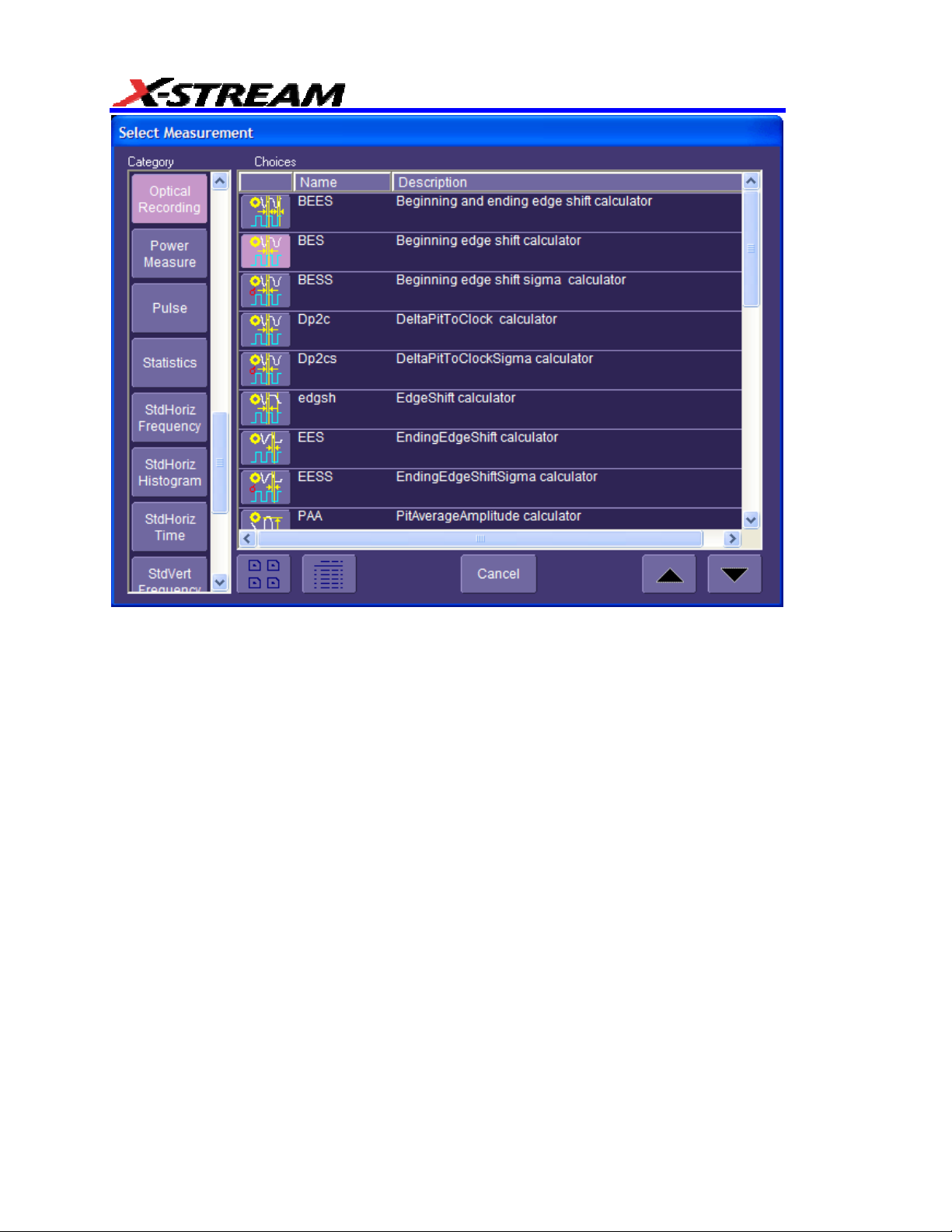
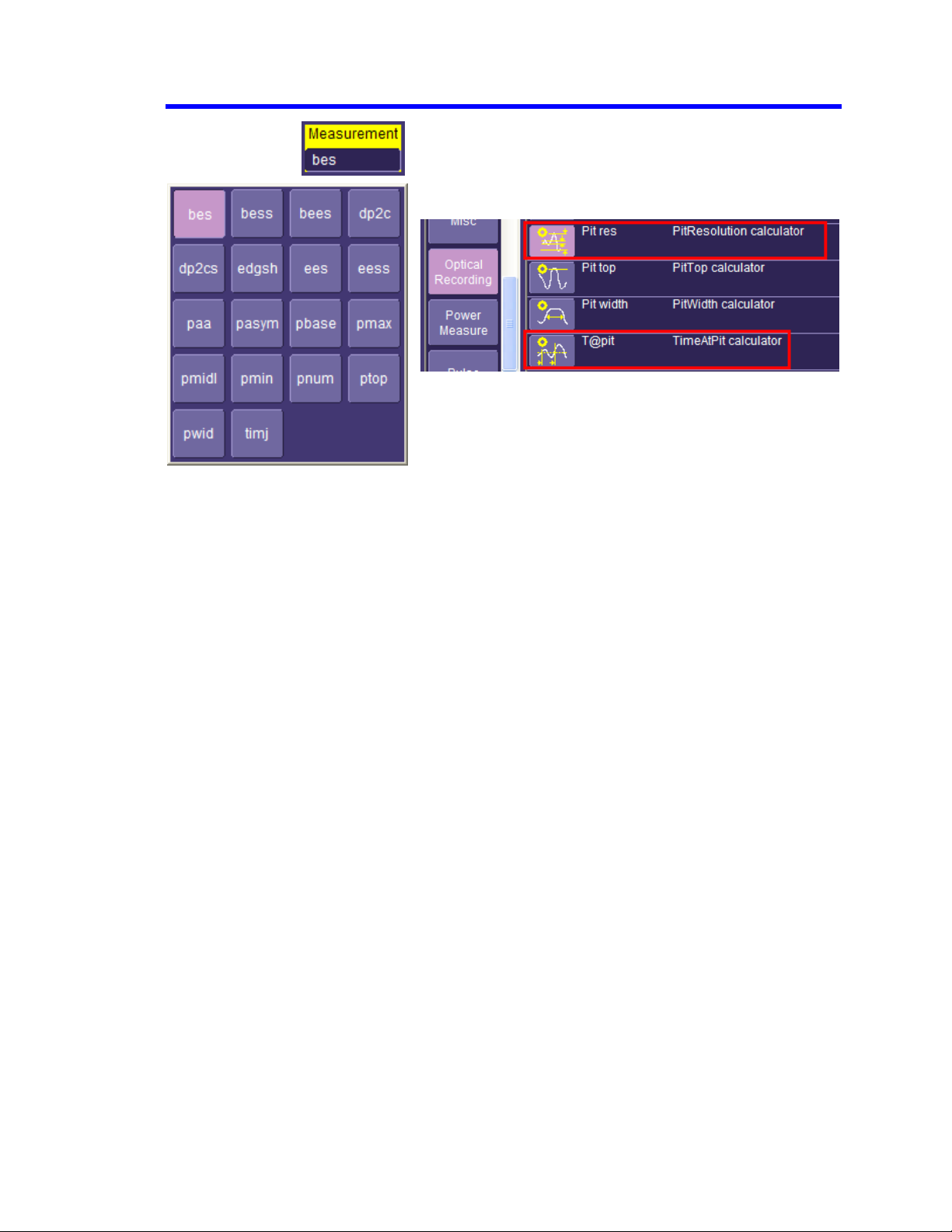
Selecting Parameters

1. Select Measure from the menu bar,

2. Touch the Px tab for the desired parameter position (P1 to P8).

3. Touch inside the Measure field, then select the Optical Recording group of parameters:

923133 Rev A ISSUED: June 2013 7

Paramete cursors. The position of the cursors can be set by dragging, entering an exact value in the

Standard Cursors dialog, or by means of the Cursors front panel knobs. When you enable

tracking by checking the Track checkbox, you can move the parameter cursors across the waveform so that measurement results can be taken on different sections of the waveform.

8 ISSUED: June 2013 923133 Rev A

rs allow measurements of the section of waveform lying between the parameter

AORM Software Package

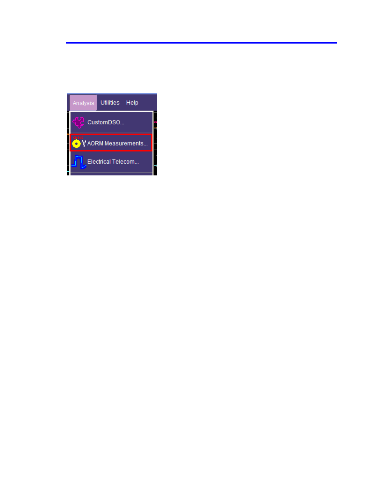
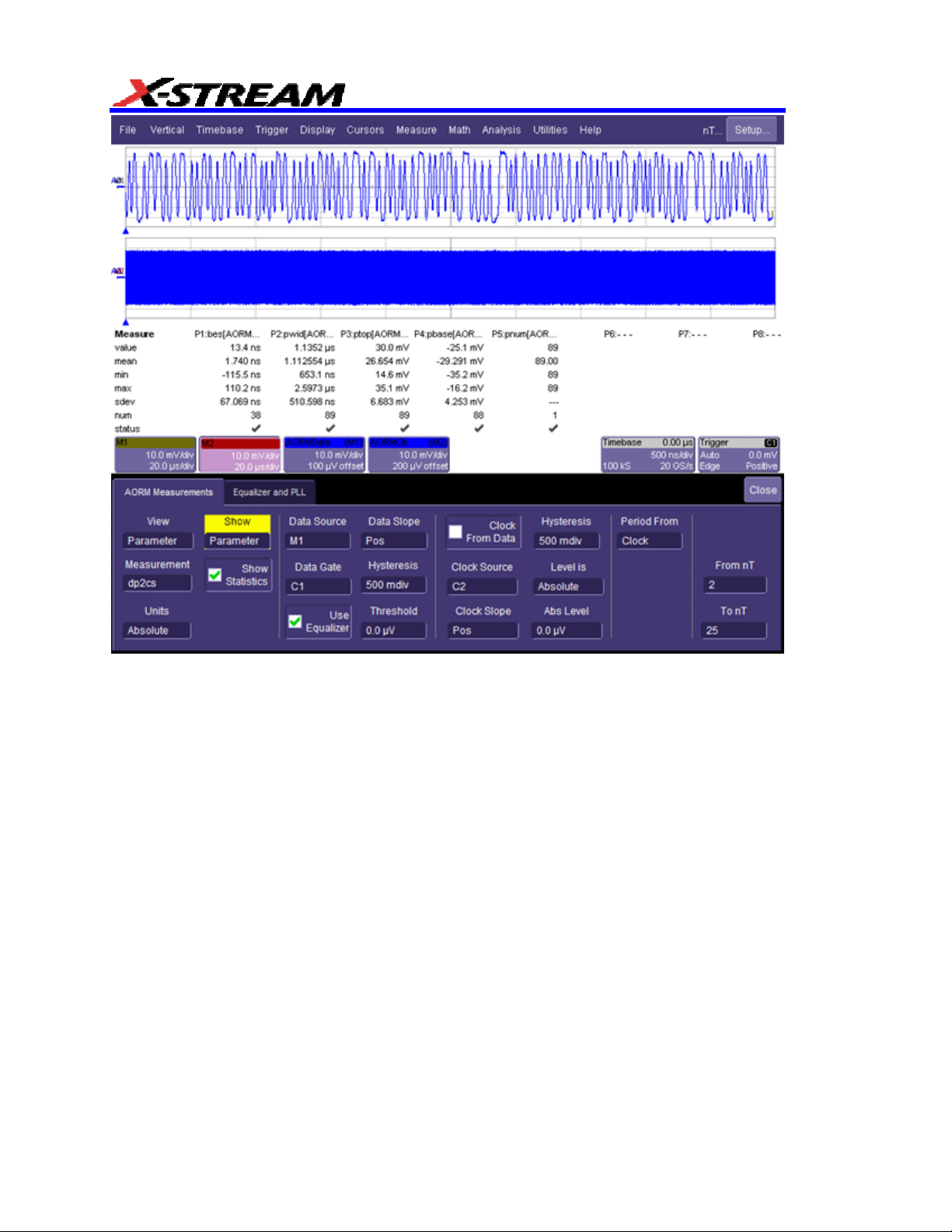
SETUP AND MEASUREMENT DIALOG

The “AORM Measurements” dialog is accessed from the menu bar’s Analysis menu. AORM is

supplied with X-Stream software version 4.2 and later. This highly interactive dialog allows you to set up and configure the clock and data sources, select a measurement type, and analyze the waveform, including statistics on parametric measurements:

923133 Rev A ISSUED: June 2013 9

10 ISSUED: June 2013 923133 Rev A

AORM Measurement Menus

Field Description

View

AORM Software Package

Measurement

Units

Allows you to

quickly select the most common views, with

graphing.

Selects the p

rimary measurement to be made. In the Parameter view, the result for the selected measurement is displayed along with other parameters.

The units u

sed for the horizontal parameter results. Absolute

refers to voltage or time units. Percent refers to results being

calculated as a percent of the clock period.

923133 Rev A ISSUED: June 2013 11

Field Description

Show

Data

Determine

s which table of values is displayed below the grid.

When Parameters is selected, a checkbox is displayed that

enables you to turn on or off the display of statistics values.

Source This can be a channel, math function, or memory

trace. A Use Equalizer checkbox is provided to

apply a filter to the data source.

Data Gate This can be a channel, math function, memory

trace, or other. It specifies the input that will be used to determine where to perform measurements on the input signal. The polarity is always high.

Use

This checkbox enables filtering of the data source.

Equalizer

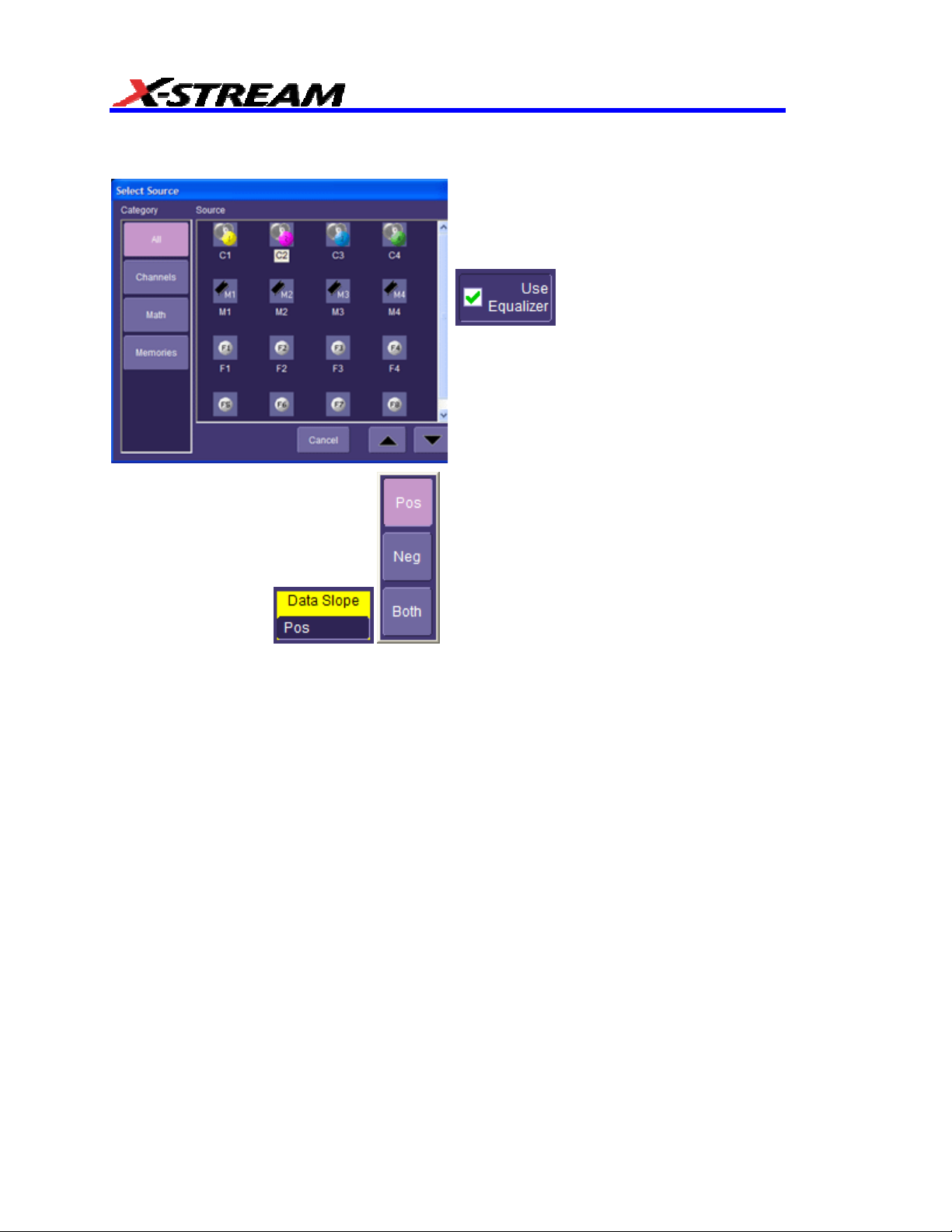
Data Slope Polarity of the pits/spaces to use for the

measurement, when appropriate. Pos polarity refers to pits, Neg polarity refers to spaces, Both

can be selected to use both pits and spaces.

Hysteresis The Hysteresis selection imposes a limit above and

below the Threshold, which precludes measurements of noise or other perturbations within this band. The width of the band is specified in divisions.

Guidelines for Use

1. Hysteresi noise spi

2. The larg than the dista

s must be larger than the ma

ke you want to ignore.

est value of hysteresis usable

nce from the threshold to the closest

ximum

is less

extreme value of the waveform.

3. Unle extreme level

ss you know the largest noise and closes

that will ever occur on any cycle,

leave some margin on both sides of the threshold.

12 ISSUED: June 2013 923133 Rev A

AORM Software Package

Field Description

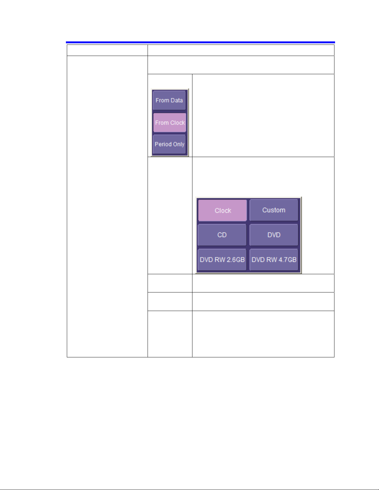
The clock need only be specified if the parameter requires a clock for the calculation, or it is used as the source of the period.

Clock/Period By selecting From Data, you can have the clock

recovered from the data. In this case, all other clock setup fields except Clock Slope are unavailable.

When From Clock is selected, the period is automatically measured from the clock provided. The clock must then be configured.

When Period Only is selected,

Clock

Period From

Indicates the period of the clock.

When a standard is selected, the period is set to the value defined by the standard. You can also set a xN multiplier (e.g., 10x).

Clock Source This can be a channel, math function, or memory

trace.

Clock Slope Choose Pos, Neg, or Near. “Near” means the

nearest clock edge to the data edge.

Hysteresis Size of the hysteresis band (in screen divisions)

with the level at the center of the band. Any waveform being analyzed must pass beyond this band before the next threshold crossing is

recognized. The Level may be set to Absolute or Percent.

923133 Rev A ISSUED: June 2013 13

Field Description

Subject nT

For BES, EES, BEES, BESS, and EESS, this specifies the pit of interest. The results will be computed for each space/pit (pit/space) pair using the subject pit and all the spaces within the range specified.

Preceded by low nT Preceded by high nT

From nT To nT

Specifies the range of n indices that define the pits/spaces used in the calculation. The range of n coupled with T are used to

categorize the pits/spaces based on their widths.

Specifies the range of n indices that define the pits/spaces used in the calculation. The range of n coupled with T is used to

categorize the pits/spaces based on their widths.

14 ISSUED: June 2013 923133 Rev A

AORM Software Package

Measurement Table

When the Parameter view is selected, up to 4 additional parameters, which are related to the selected

measurement, are displayed. The following table shows these additional parameters. For parameters that can be shown in the XY display, it also shows the parameter that is used for the X axis.

Measurement Parameters XY

(setup for custom parameters) (x axis)

dp2c (s) t@pit,pwid,pnum t@pit

EDGESH t@pit,pwid,pnum t@pit

EES (s) pwid,ptop,pbase,pnum n/a

BES (s) pwid,ptop,pbase,pnum n/a

PAA pwid,ptop,pbase,pnum n/a

Pit width t@pit, ptop,pbase,pnum t@pit

timj t@pit, ptop,pbase,pnum t@pit

Pit base pwid,ptop,pbase,pnum pwid

Pit top pwid,ptop,pbase,pnum pwid

Pit minimum pwid,ptop,pbase,pnum pwid

Pit middle pwid,ptop,pbase,pnum pwid

Pit asym pwid,ptop,pbase,pnum n/a

Pit max pwid,ptop,pbase,pnum pwid

Pit num pwid,ptop,pbase n/a

923133 Rev A ISSUED: June 2013 15

View Menu Selections

View Displays Additional Keys

Parameter

Histogram

Trend

XY Plot

The source traces will be displayed along with the custom parameters (see Measurement Table, next). If two traces are to be displayed, dual grids will be drawn.

When Histogram is selected, a

histogram of the selected parameter is displayed in a second grid, and a new tab, “AORM Histogram,” appears.

When Trend is selected, a trend plot

of the selected parameter is displayed in a second grid, and a new tab, “AORM Trend,” appears.

Plots the trend of the selected measurement vs. either the trend t@pit or pwid, as appropriate; not available for all measurements (see Measurement Table, next, for details).

When XY Plot is selected, a trend

plot of the selected parameter is displayed in a second grid, and a new tab, “AORM Trend Y,” appears.

Statistics: toggles the parameter

statistics on/off.

Find Center And Width: determines

the best scaling for the histogram based on up to the last 20,000 samples collected. This occurs automatically if the Enable Auto Find checkbox is checked.

Find Scale: determines the best

scaling for the trend (center and height). This occurs automatically if the Auto Find Scale checkbox is checked.

Find Scale: determines the best

scaling for trends (center and height). This occurs automatically if the Auto Find Scale checkbox is checked.

16 ISSUED: June 2013 923133 Rev A

Equalizer and PLL Dialog

Field Description

AORM Software Package

Track Clock

Filter Cutoff and Boost

Slicer Bandwidth

PLL Bandwidth

PLL Startup Period From

Check this checkbox to enable tracking.

An equalizer filter is applied prior to the measurements. You can adjust the cutoff frequency and boost of the filter.

The data passes through a slicer to level the data (removes the threshold due to low frequency effects). You can set the bandwidth of the slicer.

If you checked the Clock From Data checkbox, a PLL is used to

recover the clock from the data waveform. In that case, the bandwidth of the PLL can be adjusted.

Auto When Auto is selected, the startup frequency will be

determined by analyzing the peaks of the input signal.

User When User is selected, you can set the startup

frequency yourself. This is useful when the startup frequency cannot be reliably determined from the input signal.

923133 Rev A ISSUED: June 2013 17

CREATING AND ANALYZING HISTOGRAMS

Selecting the Histogram Function

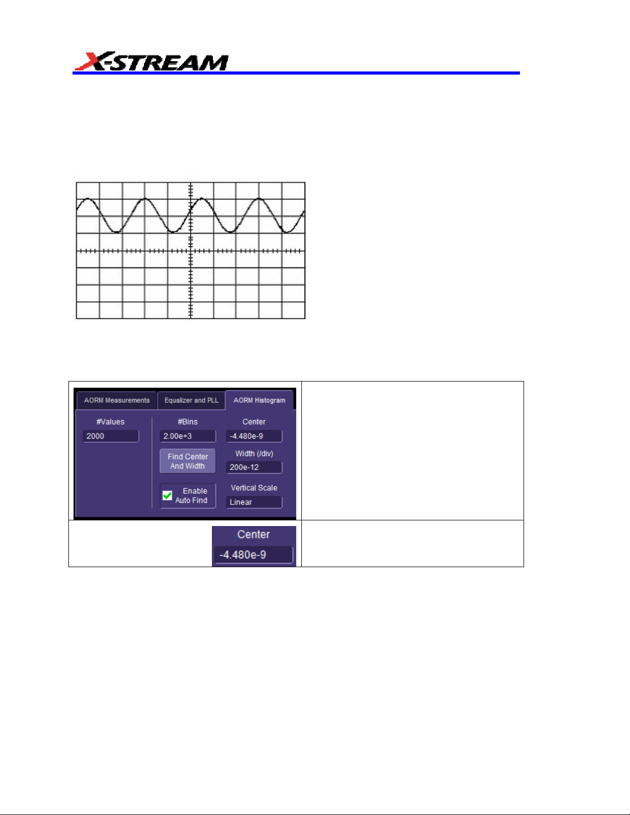
Histograms are created by graphing a series of waveform parameter measurements. The first step is to define the waveform parameter to be histogrammed. The next figure shows a screen display accompanying the selection of a frequency (freq) parameter measurement for a sine wave on Channel 1.

Four

waveform cycles are shown, which will provide four freq parameter values for each histogram on each sweep. With a freq parameter selected, a histogram based on it can be specified.

Histogram Trace Setup Dialog

Each time a waveform parameter value is calculated it can be placed in a histogram bin.

Enter the #Bins from 20 to 2000.

You can set from 20 to 2 billion parameter value calculations for histogram display in the

#Values field.

18 ISSUED: June 2013 923133 Rev A

AORM Software Package

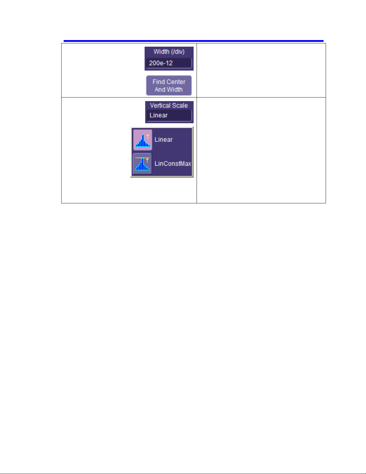
The current horizontal per division setting for the histogram. The unit type used is determined by the waveform parameter type that the histogram is based on.

The vertical scale.

• Linear make

linear. Th desi

gnates a bin value of 0.

nts increase beyond th

cou can be displayed on screen using the curre

nt vertical scale, this

automatically increa

uence.

seq

s the vertical scale

e baseline of the histog

As the bin

at which

scale is

sed in a 1-2-

ram

• LinConstMax sets the vertical scalin

to a linear val full vertical di

ue that uses clos

splay capability of

e to the

the scope. The height of the histogram will rem

ain al

most constant.

Setting Binning and Histogram Scale

For either the Linear or LinConstantMax vertical scale option, the scope automatically increases

the vertical scale setting as required, ensuring that the highest histogram bin does not exceed the vertical screen display limit.

The Center and Width fields allow specification of the histogram center value and width per

division. The width per division multiplied by the number of horizontal display divisions (10)

determines the range of parameter values centered on the number in the Center field, used to

create the histogram.

923133 Rev A ISSUED: June 2013 19

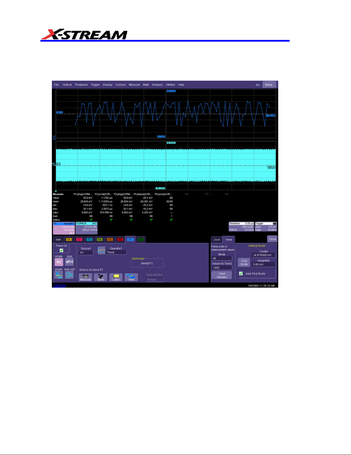
DISPLAYING TRENDS

The Trend function for processing waveforms creates a graph of successive waveform parameter values. It provides useful visual information on waveform parameter variation. Used together with other scope features, it allows you to graph certain parameters compared to others.

To Con

20 ISSUED: June 2013 923133 Rev A

figure a Trend:

From the menu bar select Math, then Math Setup… from the drop

2. Touch default).

3. Touch

an Fx tab that is not currently assigned a math function (i.e., Zoom function

inside the Source1 field and select a source waveform from the pop-up

-down menu.

menu.

AORM Software Package

4. Touch inside the Operator1 field and select Trend Opera

tor pop-up menu. The "Trend" setup dialog will appear at the right of the screen

Decide whether all the parameter values, all per trace, or only the averag para

meter calculations for each waveform acquisition should be placed in the tre

All -- every p Av

erage -- trends only the average of all the values calculated on a given acquisition an

yields on

All per Trace -- for ea

cal

culations from the new data in the trend. Unless this is specifically required, All shou

ected.

be sel

arameter calculation on each waveform will be placed

e point in the trend per acqui

sition.

ch acquisition, clears the buffer and places all param

from the Select Math

e of all

nd.

in the trend.

eter

Choose the number of values to be placed in the generated trend.

If desired, you can also configure the center and heig

7. the para used to center the trend after it has been

Cen

asso while u

Height/di

the para

923133 Rev A ISSUED: June 2013 21

meter being trended. However, this is not a requirement, and Find Scale can be

calculated.

ter is for selecting the mantissa, exponent, or number of digits resolution, us

ciated knob. The configuration is the value at the horizontal center line on th

nits are those of the parameter trende

v selects the vertical value of each vertical screen division. Units ar

meter trend

ed.

ht of the trend in the base units of

ing the

e grid,

e those of

Trend Calculation

Once the trend has been configured, parameter values will be calculated and trended on each subsequent acquisition. Immediately following an acquisition, its trend values will be calculated. The resulting trend is a waveform of data points that can be used the same way as any other

waveform. Parameters can be calculated on it, and it can be zoomed, serve as the x or y trace in

an XY plot, and can be used in cursor measurements.

The sequence for acquiring trend data is:

1. trigger

2. waveform acquisition

3. parameter calculations

4. trend update

5. trigger rearm

If the timebase is set in non-segmented mode, a single acquisition occurs prior to parameter calculations. However, in segment mode, an acquisition for each segment occurs prior to parameter calculations. If the source of trend data is a memory, storing new data to memory effectively acts as a trigger and acquisition. Because updating the screen can take significant processing time, it occurs only once a second, minimizing trigger dead time (under remote control the display can be turned off to maximize measurement speed).

Parameter Buffer

The parameter buffer allows you to include up to one million values in the trend calculation.

Parameter Events Capture

The number of events captured per waveform acquisition or display sweep depends on the parameter type. Acquisitions are initiated by the occurrence of a trigger event. Sweeps are equivalent to the waveform captured and displayed on an input channel (1, 2, 3, or 4). For nonsegmented waveforms, an acquisition is identical to a sweep. Whereas for segmented waveforms, an acquisition occurs for each segment, and a sweep is equivalent to acquisitions for all segments. Only the section of a waveform between the parameter cursors is used in the calculation of parameter values and corresponding trend events.

Reading Trends

A trend is like any other waveform: its horizontal axis is in units of events, with earlier events in the leftmost part of the waveform and later events to the right. And its vertical axis is in the same units as the trended parameter. When the trend is displayed, trace labels appear in their customary place on the screen identifying the trace, the math function performed, and giving

horizontal and vertical information:

• # number of events per horizontal division

• Units per vertical division, in units of the parameter being measured

22 ISSUED: June 2013 923133 Rev A

AORM Software Package

•

Vertical value at point in trend at cursor location when using cursors

•

Number of events in trend that are within unzoomed horizontal display range.

• Percentage of values lying beyond the unzoomed vertical range when not in cursor measurement mode.

923133 Rev A ISSUED: June 2013 23

MAKING OPTICAL DATA MEASUREMENTS

View Modes

The two modes available for Optical Recording Measurements, “Custom” and “List by nT,” both display measurements either as waveform parameters or as a list of values. This chapter further describes these modes. The following table indicates which measurements can be made in each mode.

Measurement Parameter nT Table

BEES x x

BES x x

BESS x x

Dp2c x x

Dp2cs x x

EES x x

EESS x x

EDGSH x x

PAA x x

Pit asym x

Pit base x x

Pit max x x

Pit middle x x

Pit minimum x x

Pit moda x

Pit number x x

Pit res x

Pit top x x

Pit width x x

T@pit x

Timj x x

24 ISSUED: June 2013 923133 Rev A

AORM Software Package

Configuration Options

All configuration options are available for each parameter, except as noted in this table:

Range of nT

Subject nT

Parameter

Dp2c

Dp2cs

BEES

BES

BESS

EES

EESS

EDGSH

PAA

Pit asym

Pit base

Pit max

Pit middle

Pit minimum

Pit moda

Pit num Pit res*

Pit top

Pit width

T@pit*

Timj x

x x

x x x x x x x x x x x x x x x x x x x x x x

* Available from Measure dialog

923133 Rev A ISSUED: June 2013 25

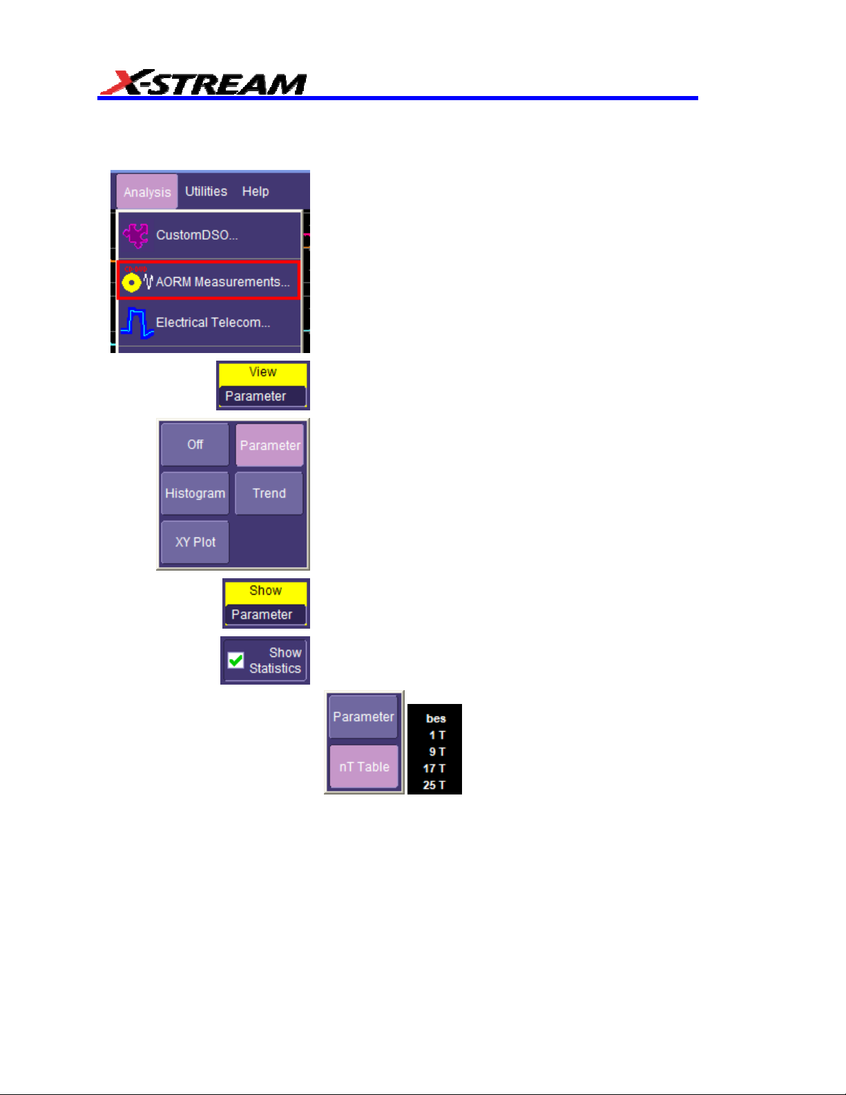
Configuration Menus

The menus described on the following pages show how to configure any parameter.

Display the AORM dial

bar at the top of the screen and selecting AORM Measurements… from the drop-down menu.

Touch insi the pop-up menu.

de the View field and select a graph display from

og by touching Analysis in the menu

Touch insi default group of parameters is automatically displayed when

Parameter is selected. In addition, if Show Statistics is

checked, standard statistics (mean, min, max, sdev, num) are also displayed.

When nT Table is selected, a default list of nT is displayed:

26 ISSUED: June 2013 923133 Rev A

de the Show field and select a display mode. A

AORM Software Package

Touch inside the Measurement field and select a

measurement from the pop-up menu. Besides the parameters included in this menu, others are available from

the Select Measurement menu, accessible from the Measure dialog:

923133 Rev A ISSUED: June 2013 27

Setting Levels

To identify pits or spaces, thresholds and hysteresis are set.

Touch inside the Data Source field and select

a signal source.

Check Use Equalizer to apply a filter to the

Data Source.

To set up the

and PLL tab.

Touch insi an edge from the pop-up menu.

equalizer, touch the Equalizer

de the Data Slope field and select

28 ISSUED: June 2013 923133 Rev A

AORM Software Package

Touch inside the Data Gate field and select a signal source. You can also select None. Data

Gate specifies the input that will be used to determine where to perform measurements on the input signal. If a Data Gate is selected, the level is assumed to be high.

The Hysteresis selection imposes a limit above and below the Threshold, which

precludes measurements of noise or other perturbations within this band. The width of the band is specified in divisions.

Select From Data from the Clock/Period menu

if you want to extract the clock from your input waveform. In this case, all other clock setup

fields become unavailable except Clock Slope. Choose Pos, Neg, or Near. “Near” means the

nearest clock edge to the data edge.

To keep noise out of parametric measurements, set up a hysteresis band, in divisions, about a level. The level can be set to

Absolute (volts) or Percent. In either case, touch inside the Abs Level or Pct Level field

and enter a value, using the pop-up keypad.

923133 Rev A ISSUED: June 2013 29

Select a clock period by having the period calculated from the clock source, by choosing a standard, or by manually setting a clock period. If you choose a clock period from a standard, you can also set a multiplier:

Setting nT

Specifies the range of n indices that define the

pits/spaces used in the calculation. The range

of n coupled with T are used to categorize the

pits/spaces based on their widths.

Maximizing Performance

A basic guideline that you should follow to maximize the performance of calculation in multiple parameter configurations is that precisely the same Value for the clock period ‘T’, Threshold level, and Hysteresis value should be used.

Following this guideline ensures that parameters can make use of results obtained in previous parameter calculations. However, in most cases there is no need for different configurations of the above three items in different parameter setups.

30 ISSUED: June 2013 923133 Rev A

AORM Software Package

Pit or Space Identification

This is determined uniquely by the threshold, hysteresis, and edge polarity of threshold crossings. A positive threshold crossing indicates the start of a positive polarity pit and the end of a negative polarity space. A positive threshold crossing followed by a negative threshold crossing fully delineates a pit. A negative crossing followed by a positive crossing fully delineates a space, as

illustrated in the following figure.

Voltage

Threshold

In order to prevent false pit and space identifications, hysteresis is provided. Hysteresis adds an additional condition that must be met before a threshold crossing is recognized as a pit/space edge. It requires that the waveform make an excursion of a certain distance from the threshold before the next threshold crossing is recognized.

The next figure shows a threshold crossing that would result in incorrect pit identification without hysteresis.

Space

False

Pit

Level

Threshold

923133 Rev A ISSUED: June 2013 31

The hysteresis band shown in the next figure is centered on the user- selected voltage level

pit

threshold.

Pit meets condition of

crossing into Zone 3

End of space.

Space fully

identified

oltage

Threshold

Zone 3

Zone 2

Zone 1

Start of pit

Pit Width

End of pit. Start

of space Pit fully

First feature

will be a

identified

Space meets condition

of crossing into Zone 1

The hysteresis band divides the display into three zones. The ORM Package uses both the voltage threshold and hysteresis settings to identify pits and spaces.

Criteria for identifying a “feature” (pit or space):

• The first feature identified after the left parameter cursor can be either a pit or space. If

the signal first enters Zone 1, the first feature identified (if additional constants are met) will be a pit. If the signal first enters Zone 3, it will be a space.

• After first crossing into Zone 1 or Zone 3, the next time the signal crosses the voltage

threshold, it is recorded as the start time of a feature.

• If the first feature to be identified is a pit (signal entered Zone 1 first), after crossing the

voltage threshold the signal must cross into Zone 3 and then pass the voltage threshold again to complete all conditions for identification as a pit. The first time that the signal crosses the voltage threshold after entering Zone 3 is recorded as the end time of the pit and the start time of the following space. The time between the start and end of the pit is recorded as the pit width. If the first feature to be identified is a space, the signal first entered Zone 3. The algorithm is used with directions reversed.

32 ISSUED: June 2013 923133 Rev A

AORM Software Package

()(

⋅+<≤⋅

−

• For the entire signal, only a space can be identified after a pit, and only a pit can be

identified after a space.

• All subsequent features are identified by crossing into the appropriate zone after the end

of the previous feature. For a pit this is Zone 3, and for a space it is Zone 1. The end of the previous feature is the beginning of the current feature being identified. The subsequent first time the signal crosses the voltage threshold is recorded as the time of the feature being identified. At this point, the feature has been fully identified.

nT Pit/Space Categorization

Because optical recording data is encoded using a pulse-width modulation mechanism, it is often useful to perform signal analysis for selected pulse widths. Exploiting the fact that optical recording data widths are ideally integral multiples of the data clock period ‘T’, the AORM Package separates optical recording signal pits and spaces into groups whose widths fall into the same integral multiple of clock periods. As a result, ORMs can be configured to provide values for only pits or spaces, or both of these for a selected ‘nT’ value (‘nT’ denotes an integer multiple of the clock period) or for a range of ‘nT’s.

The ideal clock period (T) is configured on the parameter nT setup.

Categorization of pits and spaces by nT based on width is done using the following equation:

)

TnwTn

5.05.0

When this condition is met, the pit or space of width w is said to belong to the n

index.

923133 Rev A ISSUED: June 2013 33

BES BEGINNING EDGE SHIFT

Description BES provides a measurement of the time between the beginning edge of the subject n in a specified

space/pit pair and the nearest specified clock edge. The measurement is calculated between the points where the data and clock signals cross selected voltage thresholds. The clock period T can be entered by the user, or measured from a user supplied clock signal, as described below.

The value calculated depends on the clock and data edges selected, as shown in the table below.

The data slope menu selects the polarity of the subject n pit/space. If Pos (positive) is selected,

the measurement is performed from the beginning edges of positive polarity pits and categorized

by the preceding space. If Neg (negative) is selected, the measurement is performed from the beginning edges of negative polarity spaces and categorized by the preceding pit. If Both is

selected, the beginning edges of both pits and spaces are used in the calculation and categorized by the preceding inverse polarity space/pit. The sizes of pits or spaces used in the measurement are also determined by the range of ‘nT’ values chosen.

CLOCK

EDGE

time between beginning edge of positive polarity

Positive

Negative

Near

The next figure shows the measurement of the beginning edge shift on a single subject 4T pit preceded by a 3T space. In this example, the clock is specified as the positive edge. For each space/pit combination, the beginning edge shift is calculated as the time difference between the beginning pit edge and the clock edge. Additionally, the measurements will be sorted by the space/pit pairs. For the positive polarity pit example shown in the figure after next, measurements t+ and tare for a single beginning edge shift measurement configured for positive edge, or negative edge. If nearest is selected, the smaller of t- or t+ is used.

subject pit and nearest positive clock edge

time between beginning edge of positive polarity subject pit and nearest negative clock edge

time between beginning edge of positive polarity subject pit and nearest clock edge

Pos Neg Both

DATA SLOPE

time between beginning edge of negative polarity subject space and nearest positive clock edge

time between beginning edge of negative polarity subject space and nearest negative clock edge

time between beginning edge of negative polarity subject space and nearest clock edge

time between beginning edge of subject pits and spaces to nearest positive clock edge

time between beginning edge of subject pits and spaces to nearest negative clock edge

time between beginning edge of subject pits and spaces and nearest clock edge

34 ISSUED: June 2013 923133 Rev A

AORM Software Package

threshold

Data

beginning edge shift

Beginning Edge Shift measurement of subject 4Tpit

Signal

Clock

Data Signal

Clock Signal

Zoom of Positive Polarity Pit Edge -- example measurement

923133 Rev A ISSUED: June 2013 35

The measurement has configurable units. If absolute time is specified, the value is simply the time

∆

=⋅⋅

−

indicated above. If percent is specified, the value of the measurement is the time normalized to the clock period:

For all pits, a valid measurement will be obtained only when both pit/space edges can be determined,

bes

100%

or t

(that is, there is a hysteresis-qualified threshold crossing beginning and ending the pit/space pair of interest between the parameter cursors), and there is a clock edge of both polarities surrounding the

leading pit or space edge between the parameter cursors.

Display Options

ORM parameter calculations can be displayed, histogrammed, and trended in a variety of ways.

DISPLAY TYPE VALUE DISPLAYED

All values of the time between beginning edge of the subject n pit

Parameter Statistics Off

Parameter Statistics On

nT Table

(space) and nearest clock edges for all subject pits (spaces) preceded by the spaces (pits) within the selected ‘nT’ range for the last acquisition.

Average, minimum, maximum, and sigma of the beginning edge shift calculated for all identified pit/space pairs within the selected ‘nT’ range for all acquisitions since the last C operation.

List of values of the average beginning edge shift for each ‘nT’ space (pit) within the selected range preceding the subject pit (space) for the last acquisition.

LEAR SWEEPS

Histogram graph of the value of the beginning edge shift

Histogram Function

calculated for all pit/space pairs within the selected ‘nT’ range for all acquisitions since the last C

LEAR SWEEPS operation.

Trend graph of the value of the beginning edge shift calculated for

Trend Function

all pit/space pairs within the selected ‘nT’ range for all acquisitions since the last C

LEAR SWEEPS operation.

36 ISSUED: June 2013 923133 Rev A

AORM Software Package

(

BESS

=⋅−

−

∑

(

BES

BESN

==−

−

∑

BESS BEGINNING EDGE SHIFT SIGM A

Description BESS provides a measurement of the mean, normalized standard deviation of the Beginning

Edge Shift measurements (see BES). When a single n is specified, or when you are in ‘nT Table’ Show mode, the value calculated for the n

standard deviation:

index is calculated using the following equation for

ESS

Beginning Edge Shift Sigma cannot be calculated for a given index n unless there are at least two Beginning Edge Shift values calculated or that n index.

When Beginning Edge Shift is configured as a custom parameter with a range of n, the value

calculated is the standard deviation of the distribution that results by normalizing each independent distribution categorized by the space (pit) nT preceding the subject pit (space). Distributions are normalized by subtracting the mean of the distribution from all of the elements in the distribution. This results in the following equation for overall Beginning Edge Shift Sigma resulting from the individually categorized Beginning Edge Shift Sigma values:

overall

Note: The value calculated by BESS will generally not be the same as the sigma of the BES measurement displayed on the parameter line when a range of n is used and statistics is on. This is because the two measurements are not the same. The BESS measurement normalizes the results for each n by subtracting the mean BES from each BES in the n

distribution. This results in a superposition of mean-centered distributions, not a superposition of 0-centered distributions contributing to BES measurements. BESS will always be less than or equal to the standard deviation of BES measurements.

)

923133 Rev A ISSUED: June 2013 37

Display Options

ORM parameter calculations can be displayed, histogrammed and trended in a variety of ways.

DISPLAY TYPE VALUE DISPLAYED

Single value of the standard deviation of the mean normalized

Parameter Statistics Off

beginning edge shift values for pits/spaces of interest for last acquisition.

Average, minimum, maximum, and sigma of the beginning edge

Parameter Statistics On

shift sigma value calculated per acquisition for all acquisitions since the last C

LEAR SWEEPS operation.

List of values of the standard deviation of the beginning edge shift

nT Table

values for each ‘nT’ spaces (pit) within the selected range preceding the subject pit (space) for the last acquisition.

Histogram of beginning edge shift sigma values calculated for

Histogram Function

each acquisition for all acquisitions since the last CLEAR SWEEPS

operation.

Trend of the beginning edge shift sigma values calculated for

Trend Function

each acquisition for all acquisitions since the last C

LEAR SWEEPS

operation.

38 ISSUED: June 2013 923133 Rev A

AORM Software Package

EES ENDING EDGE SHIFT

Description EES provides a measurement of the time between the ending edge of the subject n in a specified

space/pit pair and the nearest specified clock edge. The measurement is calculated between the points where the data and clock signals cross selected voltage thresholds. The clock period T can be entered by the user or measured from a user supplied clock signal, as described below.

The value calculated depends on the clock and data edges selected, as shown in the table below.

The Data Slope menu selects the polarity of the subject n pit/space. If Pos (positive) is selected,

the measurement is performed from the ending edges of positive polarity pits and categorized by

the following space. If Neg (negative) is selected, the measurement is performed from the ending edges of negative polarity spaces and categorized by the following pit. If Both is selected, the

ending edges of both pits and spaces are used in the calculation and categorized by the following inverse polarity space/pit. The sizes of pits or spaces used in the measurement are also determined by the range of ‘nT’ values chosen.

CLOCK

EDGE

Positive

Negative

Near

The next figure demonstrates the measurement of the ending edge shift on a single subject 4T pit followed by a 3T space. In this example, the clock is specified as the positive edge. For each pit/space combination, the ending edge shift is calculated as the time difference between the ending pit edge and the clock edge. Additionally, the measurements will be sorted by the pit/space pairs. For the positive polarity pit example shown in the figure after next, the measurements t+, and t- are for a single ending edge shift measurement configured for positive edge, or negative edge. If nearest is selected the smaller of t- or t+ is used.

time between ending edge of positive polarity subject pit and nearest positive clock edge

time between ending edge of positive polarity subject pit and nearest negative clock edge

time between ending edge of positive polarity subject pit and nearest clock edge

Pos Neg

DATA SLOPE

time between ending edge of negative polarity subject space and nearest positive clock edge

time between ending edge of negative polarity subject space and nearest negative clock edge

time between ending edge of negative polarity subject space and nearest clock edge

Both

time between ending edge of subject pits and spaces to nearest positive clock edge

time between ending edge of subject pits and spaces to nearest negative clock edge

time between ending edge of subject pits and spaces and nearest clock edge

923133 Rev A ISSUED: June 2013 39

threshold

Data

Signal

Clock

Signal

ending

edge shift

Ending Edge Shift measurement of subject 4T pit

Data Signal

Clock Signal

Zoom of Positive Polarity Pit Ending Edge -- example

40 ISSUED: June 2013 923133 Rev A

AORM Software Package

∆

⋅

−

For all pits, a valid measurement will be obtained only when both pit/space edges can be determined

ees t

or t

ending pit or space edge between the parameter cursors.

Display Options

ORM parameter calculations can be displayed, histogrammed, and trended in a variety of ways.

DISPLAY TYPE VALUE DISPLAYED

All values of the average time between ending edge of the subject

Parameter Statistics Off

n pit (space) and nearest clock edges for all subject pits (spaces)

followed by the spaces (pits) within the selected ‘nT’ range for the last acquisition.

100%

Average, minimum, maximum, and sigma of the ending edge shift

Parameter Statistics On

calculated for all identified pits/spaces pairs within the selected ‘nT’ range for all acquisitions since the last C

LEAR SWEEPS

operation.

List of values of the average ending edge shift for each ‘nT’ space

nT Table

(pit) within the selected range following the subject pit (space) for the last acquisition.

Histogram graph of the value of the ending edge shift calculated

Histogram Function

for all pit/space pairs within the selected ‘nT’ range for all acquisitions since the last C

LEAR SWEEPS operation.

Trend graph of the value of the ending edge shift calculated for all

Trend Function

923133 Rev A ISSUED: June 2013 41

pit/space pairs within the selected ‘nT’ range for all acquisitions since the last C

LEAR SWEEPS operation.

EESS ENDING EDGE SHIFT SIGMA

(

EESS

EES

−

∑

EES

(

⋅−−

∑

Description EESS provides a measurement of the mean, normalized standard deviation of the Ending Edge

Shift measurements (see EES). When a single n is specified, or when you are in ‘nT Table’ Show mode, the value calculated for the n

deviation:

index is calculated using the following equation for standard

Ending Edge Shift Sigma cannot be calculated for a given index n unless there are at least two Ending Edge Shift values calculated for that n index.

When Ending Edge Shift is configured as a custom parameter with a range of n, the value

calculated is the standard deviation of the distribution that results by normalizing each independent distribution categorized by the space (pit) nT following the subject pit (space). Distributions are normalized by subtracting the mean of the distribution from all of the elements in the distribution. This results in the following equation for overall Ending Edge Shift Sigma resulting from the individually categorized Ending Edge Shift Sigma values:

overall

ESS

Note: The value calculated by EESS will generally not be the same as the sigma of EES measurement when a range of

n is used and statistics are on. This is because the two measurements are not the same. The EESS measurement normalizes the results for each n by subtracting the mean EES from each EES in the n

superposition of mean-centered distributions, not a superposition of 0-centered distributions contributing to EES measurements. EESS will always be less than or equal to the standard deviation of EES measurements.

)

ESS

)

distribution. This results in a

42 ISSUED: June 2013 923133 Rev A

AORM Software Package

Display Options

ORM parameter calculations can be displayed, histogrammed and trended in a variety of ways.

DISPLAY TYPE VALUE DISPLAYED

Single value of the standard deviation of the mean normalized

Parameter Statistics Off

Parameter Statistics On

nT Table

Histogram Function

Trend Function

ending edge shift values for pits/spaces of interest for last acquisition.

average, minimum, maximum, and sigma of the ending edge shift sigma value calculated per acquisition for all acquisitions since the

LEAR SWEEPS operation.

last C

List of values of the standard deviation of the ending edge shift values for each ‘nT’ spaces (pit) within the selected range following the subject pit (space) for the last acquisition.

Histogram of ending edge shift sigma values calculated for each acquisition for all acquisitions since the last CLEAR SWEEPS

operation.

Trend of the ending edge shift sigma values calculated for each acquisition for all acquisitions since the last CLEAR SWEEPS

operation.

923133 Rev A ISSUED: June 2013 43

BEES BEGINNING ENDING EDGE SHIFT

Description BEES provides a measurement of both the beginning and ending edge shift for a subject n pit

(space) preceded and followed by a specified space (pit). (See BES and EES.) The

measurement is calculated between the points where the data and clock signals cross selected voltage thresholds. The clock period T can be entered by the user, or measured from a user supplied clock signal, as described below.

The value calculated depends on the clock and data edges selected, as shown in the table below.

The Data Slope menu selects the polarity of the subject n pit/space. If Pos (positive) is selected,

the measurement is performed from the beginning and ending edges of positive polarity pits and

is preceded and followed by a space of the specified width. If Neg (negative) is selected, the

measurement is performed from the edges of negative polarity spaces and is preceded and followed by a pit of the specified width.

CLOCK

EDGE

Positive

Negative

Near

DATA SLOPE

Pos Neg

times between edges of positive polarity subject pit and nearest positive clock edge

times between edges of positive polarity subject pit and nearest negative clock edge

times between edges of positive polarity subject pit and nearest clock edge

times between edges of negative polarity subject space and nearest positive clock edge

times between edges of negative polarity subject space and nearest negative clock edge

times between edges of negative polarity subject space and nearest clock edge

44 ISSUED: June 2013 923133 Rev A

AORM Software Package

∆

=⋅⋅

−

The next figure demonstrates the measurement of the beginning edge shift on a single subject 4T pit preceded and followed by a 3T space. In this example, the clock is specified as the positive edge. The beginning edge shift is calculated as the time difference between the beginning pit edge and the clock edge while the ending edge shift is calculated as the time difference between the ending pit edge and the clock edge.

threshold

Data

Signal

Clock

Signal

beginning edge shift

Beginning and Ending Edge Shift measurement of subject 4T pit

The measurement has configurable units. If absolute time is specified, the value is simply the time, as indicated above. If percent is specified, the value of the measurement is the time normalized to the clock period:

bees

ending

edge shift

100%

or t

For all pits, a valid measurement will be obtained only when both edges of the leading and trailing

pits/spaces can be determined (that is, there is a hysteresis-qualified threshold crossing

beginning the start pit/space and ending the end pit/space of interest between the parameter cursors), and there is a clock edge of both polarities surrounding the leading pit or space edge

between the parameter cursors.

923133 Rev A ISSUED: June 2013 45

Display Options

ORM parameter calculations can be displayed, histogrammed, and trended in a variety of ways.

DISPLAY TYPE VALUE DISPLAYED

Single value of the average time between the edges of the subject

Parameter Statistics Off

n pit (space) and nearest clock edges for all subject pits (spaces)

that are preceded and followed by the specified space (pits) for the last acquisition.

Average, minimum, maximum, and sigma of the beginning and

Parameter Statistics On

ending edge shift calculated for all subject pits (spaces) that are preceded and followed by the specified space (pits) for all acquisitions since the last C

LEAR SWEEPS operation.

List of values of the beginning edge shift and the ending edge shift

nT Table

for all subject pits (spaces) that are preceded and followed by the specified space (pits) for the last acquisition.

Histogram graph of the values of the beginning and ending edge

Histogram Function

shift calculated for all subject pits (spaces) that are preceded and followed by the specified space (pits) for all acquisitions since the

LEAR SWEEPS operation.

last C

Trend graph of the value of the beginning and ending edge shift

Trend Function

calculated for all subject pits (spaces) that are preceded and followed by the specified space (pits) for all acquisitions since the

LEAR SWEEPS operation.

last C

XY Plot

XY Plot displays the trend of one parameter vs. another.

46 ISSUED: June 2013 923133 Rev A

AORM Software Package

DP2C DELTA PIT TO CLOCK

Description Dp2c provides a measurement of the time between the leading edge of the pit (or spaces of

interest) and the nearest specified clock edge. The measurement is calculated between the points where the data and clock signals cross selected voltage thresholds.

The value calculated depends on the clock and data edges selected, as shown in the table below.

If in the Data Slope menu Pos (positive) is selected, the measurement is performed from the leading edges of positive polarity pits. If Neg (negative) is selected, the measurement is performed from the leading edges of negative polarity spaces. And if Both is selected, the

leading edges of both pits and spaces are used in the calculation. The sizes of pits or spaces used in the measurement are also determined by the range of ‘nT’ values chosen.

CLOCK

EDGE

time between leading edge of positive polarity

positive

negative

near

For the positive polarity pit example shown as the zoom of the measurement (next two figures), the measurements t+, t-, tn are for a single Delta Pit-to-Clock measurement configured for positive edge, negative edge, or nearest edge, respectively.

pit and nearest positive clock edge

time between leading edge of positive polarity pit and nearest negative clock edge

time between leading edge of positive polarity pit and nearest clock edge

Pos Neg

DATA SLOPE

time between leading edge of negative polarity space and nearest positive clock edge

time between leading edge of negative polarity space and nearest negative clock edge

time between leading edge of negative polarity space and nearest clock edge

Both

time between leading edge of pits and spaces to nearest positive clock edge

time between leading edge of pits and spaces to nearest negative clock edge

time between leading edge of pits and spaces and nearest clock edge

923133 Rev A ISSUED: June 2013 47

Delta Pit-to-Clock measurement

Data Signal

Clock Signal

Data Signal

Clock Signal

tn, t

Tn, T

Zoom of Positive Polarity Pit Edge - example measurement

48 ISSUED: June 2013 923133 Rev A

AORM Software Package

The measurement has configurable units. If absolute time is specified, the value is simply the time as indicated above. If percent is specified, the value of the measurement is the time normalized to the local clock period. The local clock period is calculated as the time between the two clock edges bracketing the clock edge used for the delta time measurement:

=⋅

∆∆

pc t

100%

or t

−

⋅

∆

100%

⋅

∆

or t

r all pits, a valid measurement will be obtained only when both pit/space edges can be determined

(that is, there is a hysteresis qualified threshold crossing that begins and ends the pit/space of interest between the parameter cursors), and when there is a clock edge of both polarities surrounding the

leading pit or space edge between the parameter cursors.

Display Options

ORM parameter calculations can be displayed, histogrammed and trended in a variety of ways.

DISPLAY TYPE VALUE DISPLAYED

All values of the average time between leading pit/space edges

Parameter Statistics Off

Parameter Statistics On

and nearest clock edges for all pits/spaces within the selected ‘nT’ range for the last acquisition.

Average, minimum, maximum, and sigma of the Delta Pit-to-Clock calculated for all identified pits/spaces within the selected ‘nT’ range for all acquisitions since the last C

LEAR SWEEPS operation.

nT Table

Histogram Function

Trend Function

923133 Rev A ISSUED: June 2013 49

List of values of the average Delta Pit-to-Clock for each group of pits/spaces of common ‘nT’ width for the last acquisition.

Histogram graph of the value of the Delta Pit-to-Clock calculated for all pits/spaces within the selected ‘nT’ range for all acquisitions since the last C

Trend graph of the value of the Delta Pit-to-Clock calculated for all pit/space within the selected ‘nT’ range for all acquisitions since the last C

LEAR SWEEPS operation.

DP2CS DELTA PIT TO CLOCK SIGMA

(

Description Dp2cs provides a measurement of the mean, normalized standard deviation of the Delta Pit-to-

Clock measurements (see Dp2c). When a single n is specified, or in ‘nT Table’ Show mode, the value calculated for the n

Delt

a Pit-to-Clock Sigma cannot be calculated for a given index n unless there are at least two Delta

Pit-to-Clock values calculated for that n index. When Delta Pit-to-Clock is configured as a custom parameter with a range of n, the value calculated is

the standard deviation of the distribution that results by normalizing each independent distribution categorized by nT. Distributions are normalized by subtracting the mean of the distribution from all of the elements in the distribution. This results in the following equation for overall Delta Pit-to-Clock Sigma resulting from the individually categorized Delta Pit-to-Clock Sigma values:

index is calculated using the following equation for standard deviation:

PCS PC

∆∆

PCS

∆

∑

∆

)

∆

()

∑

−

PCS N

∆∆PCS

overall

Note: The value calculated by DP2CS will generally not be the same as the sigma of DP2C measurement displayed on the parameter line when a range of n is used and statistics is on. This is because the two measurements are not the same. DP2CS measurement normalizes the results for each n by subtracting the mean DP2C from each DP2C in the n

distribution. This results in a superposition of mean centered distributions, not a superposition of 0 centered distributions contributing to DP2C measurements. DP2CS will always be less than or equal to the standard deviation of DP2C measurements.

50 ISSUED: June 2013 923133 Rev A

∑

⋅−

()

−

)

AORM Software Package

Display Options

ORM parameter calculations can be displayed, histogrammed, and trended in a variety of ways.

DISPLAY TYPE VALUE DISPLAYED

Single value of the standard deviation of the mean normalized

Parameter Statistics Off

Parameter Statistics On

nT Table

Histogram Function

Trend Function

Delta Pit-to-Clock values for pits/spaces of interest for last acquisition.

Average, minimum, maximum and sigma of the Delta Pit-to-Clock sigma value calculated per acquisition for all acquisitions since the

LEAR SWEEPS operation.

last C

List of values of the standard deviation of the Delta Pit-to-Clock values for each individual ‘nT’ in the selected range of ‘nT’ for the last acquisition.

Histogram of Delta Pit-to-Clock sigma values calculated for each acquisition for all acquisitions since the last CLEAR SWEEPS

operation.

Trend of the Delta Pit-to-Clock sigma values calculated for each acquisition for all acquisitions since the last CLEAR SWEEPS

operation.

923133 Rev A ISSUED: June 2013 51

EDGSH EDGE SHIFT

(

⋅+<≤⋅

∑

(

∑

Description

Edge Shift provides a measurement of the difference between the width of pits, spaces, or both, and their ideal widths. These ideal widths are integer multiples of the clock period ‘T’. The width of the pit or space is determined by the time between crossings of the selected voltage threshold

(see pwid). When a single n is specified for the Edge Shift custom parameter, for each pit-width value calculated,

the Edge Shift is calculated as:

()

wh Thus:

wh exactly the ideal T.

For ‘nT Table’ Show mode, or custom mode with one n specified, the value displayed for the n

is the average of all of the edge shift values calculated that belong to that index:

Wh parameter with a range of n, the overall edge shift is calculated and displayed as the weighted average of the edge shift values calculated above:

is the n that makes the width closest to nT (i.e., n is the n category to which the width belongs).

ere n

ere T is the configured period. It is very important for this parameter calculation that you enter

edgsh

is the number of pits belonging to the n

ere N

Tnwedgsh

⋅−= when absolute time units are specified

iii

Tnwedgsh

⋅⋅−=

iii

()

− 5.05.0

⎛ ⎜

⎜ ⎝

edgsh

overall

%0.100

when percent is specified,

)

iii

⎞ ⎟

⋅−=

⎟ ⎠

index. When edge shift is configured as a custom

∑

TnwTn

⋅

%0.100

)

Nedsh

⋅

index

The meas JTC1.23.14517 Section 22.4.

Display Options

ORM parameter calculations can be displayed, histogrammed, and trended in a variety of ways.

52 ISSUED: June 2013 923133 Rev A

urement calculation is compliant with the definition of Edge Shift as defined by ISO/IEC

AORM Software Package

DISPLAY TYPE VALUE DISPLAYED

Parameter Statistics Off

Parameter Statistics On

nT Table

Histogram Function

Trend Function

Example

The example shows the CD data signal measured at the selected voltage threshold containing, in sequence, a 5T pit, 3T space, 3T pit and 4T space. If the clock period ‘T’ is 231.5 ns, then the 5T and 4T edge shift value is simply the difference between the width calculated and the ideal width (since there is only one pit/space of that ‘nT’ width), thus:

edgsh T

All values of the overall edge shift for all pits/spaces within the selected ‘nT’ range for last acquisition.

Average, minimum, maximum, and sigma of all edge shift values calculated per acquisition for all acquisitions since the

LEAR SWEEPS operation.

last C

List of values of the overall edge shift for each group of pits/spaces of common ‘nT’ width for the last acquisition.

Histogram of the single overall edge shift value calculated for each acquisition for all acquisitions since the last CLEAR SWEEPS

operation.

Trend of the single overall Edge Shift value calculated for each acquisition for all acquisitions since the last CLEAR SWEEPS

operation.

() .

4 920 4 2315

() .

5 1160 5 2315

()

=−⋅ ⋅ =−

()

=−⋅⋅ =+

100%

2315 100%

2315

259%

108%

The 3T ed

ge shift value is the average difference:

⎛

()()

⎜ ⎝

−⋅ ⋅

690 3 2315

100%

edgsh T()

⎛

⎞

⎜

⎟+ − ⋅ ⋅

695 3 2315

⎝

⎠

2315

100%

2315

⎞ ⎟ ⎠

086%=

In an nT Table display, these three values would be shown in the appropriate nT location.

923133 Rev A ISSUED: June 2013 53

More On Edge Shift

A good approach to understanding the operation of the edge shift parameter with different modes of operation starts by considering the next figure, a histogram of 3T to 5T pit widths.

voltage

threshold

1.16 µs

690

695

920 ns

Histogram of Pit Widths

600

400

Population

200

2.5 3 3.5 4 4.5 5 5.5 Pit Width / T

3T Widths 4T Widths 5T Widths

The E

dge Shift parameter takes on each of these distributions separately. For each distribution, the ideal width (nT) is subtracted from the pit widths and the difference is calculated in percent. As a result, the Edge Shift distributions are calculated, shown in the next figure.

54 ISSUED: June 2013 923133 Rev A

AORM Software Package

800

600

400

Population

200

30 20 10 0 10 20 30

Edge Shift in Percent

3T Edge Shift 4T Edge Shift 5T Edge Shift Superposition of Edge Shift Distributions

Histogram of Edge Shifts

3T, 4T, and 5T distributions are obtained when the Edge Shift custom parameter is configured for

The

single n values and histogrammed. The final superposition distribution is obtained when the Edge Shift custom parameter is configured for ranges of n values (in this case 3T to 5T) and histogrammed.

The value displayed on the custom parameter line (with statistics off) is the mean of any of the resulting

distributions for the last acquisition only. This average edge shift value is calculated internally without

actually histogramming the values. The values displayed in ‘nT Table’ mode are the mean of the Edge

Shift distributions resulting from each nT distribution f or the last ac quisition.

Note: The standard deviation of superimposed Edge Shift distributions is not the same as Timing Jitter.

923133 Rev A ISSUED: June 2013 55

PAA PIT AVERAGE AMPLITUDE

Description

Pit Average Amplitude provides a measurement of the average amplitude of pits and spaces. The calculation is performed by calculating the difference between the average value of the base (pbase) for spaces of a particular ‘nT’ width and the average value of the top (ptop) of pits of the same ‘nT’ width. For example, the average value of the base for all 3T spaces is subtracted from the average value of the top for all 3T pits to obtain the 3T pit average amplitude. If a range of ‘nT’ values is selected and is displayed as a parameter, the measurement provides the weighted average amplitude based on the number of occurrences of each ‘nT’ pit/space width.

Display Options

ORM parameter calculations can be displayed, histogrammed, and trended in a variety of ways.

DISPLAY TYPE VALUE DISPLAYED

Parameter Statistics Off

Parameter Statistics On

nT Table

Histogram Function

Trend Function

Single value of the average amplitude for all pits/spaces of interest for last acquisition.

Overall average, minimum, maximum, and sigma of the single average amplitude value calculated per acquisition for all acquisitions since the last C

LEAR SWEEPS operation.

List of the average amplitude values for each group of pits/spaces of common ‘nT’ width for the last acquisition.

Histogram of the single average amplitude value calculated for each acquisition for all acquisitions since the last C

LEAR SWEEPS operation.

Trend of the single average amplitude value calculated for each acquisition for all acquisitions since the last C

LEAR SWEEPS operation.

56 ISSUED: June 2013 923133 Rev A

Example

Consider this persistence plot of an optical data waveform. Using cursors, the average amplitude of the 3T pits/spaces can be estimated. In this case, the value obtained is 47.2 mV.

When the parameter paa is configured for 3T widths, the measurement result is also 47.2 mV. This value is calculated automatically.

AORM Software Package

923133 Rev A ISSUED: June 2013 57

PASYM PIT ASYMMETRY

−

Description

Pit Asymmetry provides a measurement of the asymmetry of the middle voltage level for the high nT index pits/spaces compared to the middle voltage level of the low ‘nT’ index pits/spaces. The measurement calculation is compliant with the definition of Pit Asymmetry as defined by IEC 908:1987 Section 3.1. The negative value of the measurement is referred to as Pit Symmetry as defined by ISO/IEC 10149:1995 (E) Section 12.2. Pit Asymmetry is calculated by the formula:

pmidl pmidl

high n low n

PASYM

re paa is the average peak-peak amplitude. The low (smallest) and high (largest) ‘nT’ values to

whe

use in performing the calculation are provided by the user through the associated measurement configuration options. Midpoint designates the midpoint value between the average top and base for a specified ‘nT.’ The value shown is in units of percent.

Display Options

ORM parameter calculations can be displayed, histogrammed, and trended in a variety of ways.

DISPLAY TYPE VALUE DISPLAYED

paa

high n

⋅

100%

Parameter Statistics Off

Single value of the asymmetry for the last acquisition.

Average, minimum, maximum and sigma of the single

Parameter Statistics On

Histogram Function

Trend Function

asymmetry value calculated per acquisition for all acquisitions since the last C

LEAR SWEEPS operation.

Histogram of asymmetry value calculated per acquisition for all acquisitions since last C

LEAR SWEEPS operation.

Trend of single asymmetry value calculated per acquisition for all acquisitions since last C

LEAR SWEEPS operation.

58 ISSUED: June 2013 923133 Rev A

Example

This persistence plot of a bandwidth limited, smooth waveform illustrates asymmetry.

Notice that the midlevel of the 3T waveform is offset from 0 V, and that the midlevel of the 11T waveform is approximately 0 V.

Since the 3T middle level is offset, the expected asymmetry value is negative. This is the asymmetry calculated from a waveform with several thousand widths. The values are the asymmetry, the 3T middle level, the 11T middle level, and the 11T average amplitude.

AORM Software Package

923133 Rev A ISSUED: June 2013 59

PBASE PIT BASE

Description

Pit Base provides a best estimate of the bottom amplitude of a space. The concept of the base calculation is to automatically provide the same measurement that would be obtained from a persistence

plot. The base of each space is determined through histogramming techniques described under Base and Top Calculation Details.

When pbase is configured as a custom parameter, all bases within the single nT or range of nT are

calculated. Histogramming or trending such a configuration would result in one value per space in the nT range contributing a value to the histogram or trend. The value displayed on the custom parameter display line is the average of all such base calculations. ‘nT Table’ mode provides an average base

measurement for each n index.

Display Options

ORM parameter calculations can be displayed, histogrammed, and trended in a variety of ways. The following table provides a concise description of the value or values displayed using each approach.

DISPLAY TYPE VALUE DISPLAYED

Parameter Statistics Off

All values of the base for all spaces within the selected ‘nT’ range for the last acquisition.

Average, minimum, maximum, and sigma of the base for all

Parameter Statistics On

nT Table

spaces that are within the selected ‘nT’ range for all acquisitions since the last C

LEAR SWEEPS operation.

List of values of the average base for each group of spaces of common ‘nT’ width for the last acquisition.

Histogram graph of the value of the base for all spaces within

Histogram Function

the selected ‘nT’ range for all acquisitions since the last C

LEAR

SWEEPS operation.

Trend graph of the value of the base calculated for space that is

Trend Function

within the selected ‘nT’ range for all acquisitions since the last

LEAR SWEEPS operation.

60 ISSUED: June 2013 923133 Rev A

Example

This persistence waveform is created by setting a SMART Trigger

to capture only 4T spaces. The 4T base computed is

-27.0 mV.

When the same measurement is taken with the parameter cursors, it confirms that

-27.0 mV is a reasonable value for the base.

AORM Software Package

923133 Rev A ISSUED: June 2013 61

PMAX PIT MAXIMUM

Description

Pit Maximum provides a measurement of the maximum voltage value of pits of interest. It

provides a comparison of how the maximum point in the waveform corresponds to the ptop value When pmax is configured as a custom parameter, all maximums within the single nT or range of

nT are calculated. Histogramming or trending such a configuration would result in one value per pit in the nT range contributing a value to the histogram or trend. The value displayed on the custom parameter display line is the average of all such maximum calculations. ‘nT Table’ mode

provides an average maximum value for the pits in each n index.

Display Options

ORM parameter calculations can be displayed, histogrammed and trended in a variety of ways. The table provides a concise description of the value or values displayed using each approach.

DISPLAY TYPE VALUE DISPLAYED

Parameter Statistics Off

Parameter Statistics On

nT Table

Histogram Function

Trend Function

All values of the maximum for all pits within the selected ‘nT’ range for the last acquisition.

Average, minimum, maximum, and sigma of the maximum for all pits that are within the selected ‘nT’ range for all acquisitions since the last C

LEAR SWEEPS operation.

List of values of the average maximum for each group of pits of common ‘nT’ width for the last acquisition.

Histogram graph of the value of the maximum for all pits within the selected ‘nT’ range for all acquisitions since the last C

LEAR

SWEEPS operation.

Trend graph of the value of the maximum calculated for each pit that is within the selected ‘nT’ range for all acquisitions since the last C

LEAR SWEEPS operation.

62 ISSUED: June 2013 923133 Rev A

Example:

This waveform contains a single pit, whose max is computed as 26.1 mV.

The same measurement is verified using the measurement cursors.

AORM Software Package

923133 Rev A ISSUED: June 2013 63

PMIDL PIT MIDDLE LEVEL

Description

Pit Middle Level provides a measurement of the middle voltage level of pits or spaces. It is

performed by first calculating the midpoint of the average value of the base (pbase) for spaces and the average value of the top of pits (ptop). If only 3T pits are specified, the resulting

measurement is the ‘decision level’ (see ISO/IEC 10149:1995 (E) Section 12.1). If a range of ‘nT’ values is selected and is displayed as a parameter, the measurement provides the weighted average midpoint based on the number of occurrences of each ‘nT’ pit/space width. The measurement value can be used to determine not only the differences of the midpoint of different

‘nT’ width pits, but also the overall best data waveform voltage threshold setting to use for all

ORMs.

Display Options

ORM parameter calculations can be displayed, histogrammed, and trended in a variety of ways.

DISPLAY TYPE VALUE DISPLAYED

Parameter Statistics Off

Parameter Statistics On

nT Table

Histogram Function

Trend Function

Single value of the middle level for all pits/spaces of interest for last acquisition.

Overall average, minimum, maximum, and sigma of the single middle level value calculated per acquisition, for all acquisitions since the last C

LEAR SWEEPS operation.

List of the middle level values for each group of pits/spaces of common ‘nT’ width for the last acquisition.

Histogram of the single middle level value calculated for each acquisition for all acquisitions since the last CLEAR SWEEPS operation.

Trend of the single middle level value calculated for each acquisition for all acquisitions since the last CLEAR SWEEPS operation.

64 ISSUED: June 2013 923133 Rev A

Example

This waveform contains thousands of pits. In ‘nT Table’ mode, the middle levels are displayed for each nT index. These values are the midlevels of the tops and bases for pits/spaces within the nT indices.

The overall middle level is calculated based on a weighted average of the middle level for each nT. This value is the overall best threshold value for all pits/spaces within the 3T to 11T range.

AORM Software Package

923133 Rev A ISSUED: June 2013 65

PMIN PIT MINIMUM

Description

Pit Minimum provides a measurement of the minimum voltage value of pits of interest, and a

comparison of how the minimum point in the waveform corresponds to the ptop value. When pmin is configured as a custom parameter, all minimums within the single nT or range of nT are

calculated. Histogramming or trending such a configuration would result in one value per pit in the nT range contributing a value to the histogram or trend. The value displayed on the custom parameter display line is the average of all such minimum calculations. ‘nT Table’ mode provides

an average minimum value for the pits in each n index.

Display Options

ORM parameter calculations can be displayed, histogrammed, and trended in a variety of ways.

DISPLAY TYPE VALUE DISPLAYED

Parameter Statistics Off

Parameter Statistics On

nT Table

Histogram Function

Trend Function

All values of the minimum for all pits within the selected ‘nT’ range for the last acquisition.

Average, minimum, maximum, and sigma of the minimum for all pits that are within the selected ‘nT’ range for all acquisitions since the last C

LEAR SWEEPS operation.

List of values of the average minimum for each group of pits of common ‘nT’ width for the last acquisition.

Histogram graph of the value of the minimum for all pits within the selected ‘nT’ range for all acquisitions since the last CLEAR SWEEPS operation.

Trend graph of the value of the minimum calculated for each pit that is within the selected ‘nT’ range for all acquisitions since the last C

LEAR SWEEPS operation.

66 ISSUED: June 2013 923133 Rev A

Example

This waveform contains a single space. The pit min is computed as -9.7 mV.

The measurement can be verified with the measurement cursors.

AORM Software Package

923133 Rev A ISSUED: June 2013 67

PMODA PIT MODULATION AMPLITUDE

Description

Pit Modulation Amplitude provides a measurement of the ratio of the Pit Average Amplitude (paa) for the low ‘nT’ pits/spaces in the data signal to the Pit Top (ptop) of the high ‘nT’ pits in the data

signal:

paa

low n

PMODA

avg top

()

high n

The low a

nd high ‘nT’ values to be used for performing the calculation are provided by the user

through the associated measurement configuration options. Some measurements of modulation

amplitude require the low and high n index to be identical. The value is shown is decimal. The

measurement calculation is compliant with the definition of Modulation Amplitude as defined by IEC 908:1987 Section 9.2 and ISO/IEC 10149:1995 (E) Section 12.2.

Note: This measurement must be performed on the DC-coupled optical data waveform, otherwise incorrect values will

result.

Display Options

ORM parameter calculations can be displayed, histogrammed, and trended in a variety of ways.

DISPLAY TYPE VALUE DISPLAYED

Parameter Statistics Off

Single value of the modulation amplitude for the last acquisition.

Average, minimum, maximum, and sigma of the single

Parameter Statistics On

modulation amplitude value calculated per acquisition for all acquisitions since the last C

LEAR SWEEPS operation.

Histogram of the modulation amplitude value calculated per

Histogram Function

acquisition for all acquisitions since the last CLEAR SWEEPS operation.

Trend of the single modulation amplitude value calculated per

Trend Function

acquisition for all acquisitions since the last C

LEAR SWEEPS

operation.

68 ISSUED: June 2013 923133 Rev A

Example

The following persistence plots were generated using the DC-coupled signal.

In the first plot, the amplitude measurement cursor is reading the 11T top voltage of 76.7 mV

AORM Software Package

923133 Rev A ISSUED: June 2013 69

In the second, the cursor reads the difference between the 11T top and base of

67.2 mV.

In the third plot, the cursor reads the difference between the 3T top and base of

47.2 mV.

70 ISSUED: June 2013 923133 Rev A

The last plot shows the waveform with the parameters calculated automatically.

1. pmoda 3T paa/11T top

2. pmoda 11T paa/11T top

3. paa 3T

4. paa 11T

5. top 11T P1 contains the ratio of

P3 to P5. P2 contains the ratio of P4 to P5.

AORM Software Package

923133 Rev A ISSUED: June 2013 71

PNUM PIT NUMBER

Description

Pit Number provides a measurement of the number of pits or spaces of interest or both. When

pnum is selected as a parameter measurement the total number of pits and/or spaces for the

selected ‘nT’ range is displayed. In the nT Table mode the number for each ‘nT’ value is displayed.

Display Options

ORM parameter calculations can be displayed, histogrammed, and trended in a variety of ways. The table provides a concise description of the value or values displayed using each approach.

DISPLAY TYPE VALUE DISPLAYED

Parameter Statistics Off

Parameter Statistics On

nT Table

Histogram Function

Trend Function

Single value of the total number of pits/spaces within the selected ‘nT’ range for the last acquisition.

Average, minimum, maximum, and sigma of the single value of the total number of pits/spaces within the selected ‘nT’ range, calculated per acquisition for all acquisitions since the last C

LEAR SWEEPS

operation.

List of values of the number pits/spaces for each individual ‘nT’ in the selected range of ‘nT’ for the last acquisition.

Histogram graph of the single value of the number of pits/spaces within the selected ‘nT’ range calculated each acquisition for all acquisitions since the last C

LEAR SWEEPS operation.

Trend graph of the single value of the number of pits/spaces within the selected ‘nT’ range calculated each acquisition for all acquisitions since the last C

LEAR SWEEPS operation.

72 ISSUED: June 2013 923133 Rev A

Example

In this waveform, each of the 3 pits/spaces is easily identified. There is a 4T pit, a 6T space, and a 5T pit. Each is counted and displayed in ‘nT Table’ mode.

AORM Software Package

This is th

e long waveform showing the number of pits/spaces obtained: approximately 9,000.

923133 Rev A ISSUED: June 2013 73

PRES PIT RESOLUTION

Description

Pit Resolution measures the ratio of the Pit Average Amplitude (see paa measurement

description) of the smallest of the ‘nT’ pits or spaces in the data signal to that of the largest:

paa

low n

PRES

=⋅

paa

w and high ‘nT’ values for performing the calculation must be provided by the user through the

The lo

associated measurement configuration options. The value shown is in units of percent. The measurement calculation is compliant with the definition of Pit Resolution as defined by IEC 13549:1993 Section 15.3.1.

Display Options

ORM parameter calculations can be displayed, histogrammed, and trended in a variety of ways. The table provides a concise description of the value or values displayed using each approach.

DISPLAY TYPE VALUE DISPLAYED

high n

100%

Parameter Statistics Off

Parameter Statistics On

Histogram Function

Trend Function

Single value of the pit resolution for the last acquisition.

Overall average, minimum, maximum, and sigma of the single pit resolution value calculated per acquisition for all acquisitions since the last C

LEAR SWEEPS operation.

Histogram of the single pit resolution value calculated per acquisition for all acquisitions since the last CLEAR SWEEPS operation.

Trend of the single pit resolution value calculated per acquisition for all acquisitions since the last C

LEAR SWEEPS operation.

74 ISSUED: June 2013 923133 Rev A

Example

Consider the following persistence plots. In the first, the amplitude measurement cursor reads the difference between the 3T top and base: 47.3 mV.

In the second, the cursor reads the difference between the 11T top and base:

67.3 mV.

AORM Software Package

Therefore, the resolution is:

923133 Rev A ISSUED: June 2013 75

This is the same waveform with the parameters calculated automatically.

1. pres 3T paa / 11T paa

2. paa 3T

3. paa 11T P1 contains the ratio

of P2 to P3 in percent.

76 ISSUED: June 2013 923133 Rev A

AORM Software Package

PTOP PIT TOP

Description

Pit Top provides a measurement of the best estimate of the top amplitude of a pit. The concept of the top calculation is to automatically provide the same measurement which would be obtained from a persistence

plot. The top of each pit is determined through histogramming techniques described in detail under Base and Top Calculation Details. When ptop is configured as a custom parameter, all tops within the single nT or

range of nT are calculated. Histogramming or trending such a configuration would result in one value per pit in the nT range contributing a value to the histogram or trend. The value displayed on the custom parameter display line is the average of all such top calculations. ‘nT Table’ mode provides an average top measurement

for each n index.

Display Options

ORM parameter calculations can be displayed, histogrammed, and trended in a variety of ways.

DISPLAY TYPE VALUE DISPLAYED

Parameter Statistics Off

Parameter Statistics On

nT Table

Histogram Function

Trend Function

All values of the top for all pits within the selected ‘nT’ range for the last acquisition.

Average, minimum, maximum, and sigma of the top for all pits within the selected ‘nT’ range for all acquisitions since last CLEAR SWEEPS operation.

List of values of the average top for each group of pits of common ‘nT’ width for the last acquisition.

Histogram graph of the value of the top for all pits within the selected ‘nT’ range for all acquisitions since the last C

LEAR SWEEPS operation.

Trend graph of the value of the top calculated for pit that is within the selected ‘nT’ range for all acquisitions since last CLEAR SWEEPS operation.

923133 Rev A ISSUED: June 2013 77

Example

This persistence waveform was created by setting a SMART Trigger to capture only 3T pits. The computed 3T top is 25.8 mV.

When the same measurement is taken with the parameter cursors, it confirms that

25.8 mV is a reasonable value for the top.

78 ISSUED: June 2013 923133 Rev A

AORM Software Package

PWID PIT WIDTH

Description

Pit Width provides a measurement of the width of pits or spaces or both. The width of the pit or

space is determined by the crossing of the selected voltage threshold. When pwid is selected as

a parameter measurement it is generally useful to display the measurement calculation for a single ‘nT’ value. Otherwise the measurement will calculate the average width of 3T pits, 4T pits, and so on, which is meaningless. However, it is also often desirable to histogram the width of all

pits and/or spaces. In this case the range of ‘nT’ values should be set to include all pit/space

widths of interest.

Display Options

ORM parameter calculations can be displayed, histogrammed, and trended in a variety of ways. The table provides a concise description of the value or values displayed using each approach.

DISPLAY TYPE VALUE DISPLAYED

Parameter Statistics Off

Parameter Statistics On

nT Table

Histogram Function

Trend Function

All values of the pit width for all pits/spaces within the selected ‘nT’ range for the last acquisition.

Average, minimum, maximum, and sigma of the pit width for all pits/spaces that are within the selected ‘nT’ range for all acquisitions since the last C

LEAR SWEEPS operation.

List of values of the average pit width for each group of pits/spaces of common ‘nT’ width for the last acquisition.

Histogram graph of the value of the pit width for all pits/spaces within the selected ‘nT’ range for all acquisitions since the last CLEAR SWEEPS operation.

Trend graph of the value of the pit width for all pits/spaces within the selected ‘nT’ range for all acquisitions since the last C

LEAR SWEEPS

operation.

923133 Rev A ISSUED: June 2013 79

Example

The example shows that, measured at the selected voltage threshold, the CD data signal contains sequentially a 5T pit, 3T space, 3T pit, and 4T space. If the measurement is configured to select only 3T pits or spaces then the value displayed will be:

pwid = (694 ns + 696 ns) / 2 = 695 ns

voltage

threshold

1.16

µs

694

696

925 ns

Example 2: Histogramming

Consider the problem of determining the error margin in an optical recording system. Because the data is encoded in the widths of the pits/spaces, it would be ideal for the widths to be exact integer multiples of the period of the clock used to sample the data signal. In practice this is not the case, but in order to ensure error-free data recovery, it is important for the widths to be grouped and separated.

Histogramming can be used to analyze the grouping of pit widths and to determine whether the separation is acceptable.

The scope is set up to acquire the optical data waveform by assigning Channel 1 to the data signal at a time/div of 0.2 ms, so that many pits/spaces can be gathered quickly. The signal is AC-coupled, so the threshold is set to 0 mV.

The pwid custom parameter is assigned to P1 and configured in the following manner:

hysteresis = 0.5 divisions threshold = 0 mV polarity = Both range of n

low n = 3 high n = 11

period = 231.5 ns.

F1 is defined as a zoom of channel 1 so that the waveform can be viewed expanded and the pits and spaces can be identified.

Using the Math Setup dialog, F2 is defined as the histogram of the pwid parameter on P1 and is

set up as follows:

80 ISSUED: June 2013 923133 Rev A

AORM Software Package

1. Use the maximum number of values (2

,000,000,000)

2. Classify into 2000 bins

3. Linear vertical scale.

The trigger is set up to trigger on a pit edge and operated in normal trigger mode.

Note: Prior to acquisition, select each trace and press the RESET button to ensure that all the traces are reset.

In normal trigger mode, multiple waveforms are acquired and processed. The histogram will

typically have data that is not well centered or is off screen. Touch the FIND CENTER AND WIDTH button to see the pit width distributions as they accumulate. After enough measurements

have been taken, stop the triggering. After the histogram has been centered, the screen will look as follows:

The optical data waveform is on the top and the histogram is on the bottom. Notice the clustering of width distributions.

923133 Rev A ISSUED: June 2013 81

By enabling cursor tracking, the difference cursors are swept across the histogram. As expected, the space between the 3T and 4T distributions is the shortest, because of inter-symbol interference and the many 3T widths. The spacing is 138 ns.

To measure the spread of widths for the distributions, set the measure mode to My Measure and

configure the parameters:

P2: average

2. P3: high of F2

of F2

3. P4: low of F2

P5: range of

se parameter measurements are performed only on those portions of the waveform

Becau between the parameter cursors, activate tracking so that they can be swept across the histogram. Set the difference between the cursors so that they encompass one clock period. In this case, the histogram is shown at 0.2 µs per division. Set the difference between the parameter cursors to:

82 ISSUED: June 2013 923133 Rev A

⋅

2315 10

−

⋅

210

−

116

divisions

This screen shows the histogram statistics taken on the 5T distribution. The distribution has the largest spread of values: 102.5 ns. The

mean is 1.1659 which is 3.6% higher than the ideal of

1.1575

AORM Software Package

923133 Rev A ISSUED: June 2013 83

T@PIT TIME AT PIT

Description

The Time-at-Pit parameter provides the time of each leading edge of every pit or space within the

nT range specified from the trigger point (time = 0). The value displayed is the time of the first pit

only.

The usefulness of this parameter is not in the displayed value, but in its trending. The intent is that two parameters (t@pit and another ORM parameter) can be set up with identical configurations: precisely the same number of pits or spaces is found in the waveform, and precisely the same number of parameter measurements is made. When both of these parameters are trended, the two trends will have the same number of events, and there will be a one-to-one correspondence between each event in each trend. If both trends are displayed, and time cursors are swept over each, values will be displayed for the ORM parameter value and the time within the acquisition where the parameter measurement was made. These times are useful when searching for abnormal events within a waveform.

Not only can the trend of t@pit provide the actual event time, it can be used as the x-axis in an

XY plot to examine modulation characteristics of particular parameter measurements.

Example

This example typifies the usage of the t@pit parameter. Step-by-step instructions are given.

A large optical recording waveform is to be acquired, and the ordinary pit/space widths that can cause errors in the system need to be found. The waveform contains pits/spaces that have widths that are ideal integer multiples of the clock period 231.5 ns in a range from 3 to 11 times this clock period.

The scope is set up to acquire this waveform by assigning Channel 1 to the data signal at a time/div of 0.2 ms. This signal will contain approximately 1800 pits/spaces. The ideal threshold

(determined by the pmidl parameter) is 1.9 mV. The pwid custom parameter is assigned to P1 and the t@pit parameter to P2. Both parameters

are configured in the following manner:

hysteresis = 0.5 divisions threshold = 1.9 mV polarity = Both range of n

low n = 0 high n = 25

period = 231.5 ns.

Using the Math Setup… dialog, define F1 as the trend of the pwid parameter, and F2 as the trend of the t@pit parameter. For later use, define F3 as a zoom of Channel 1.

84 ISSUED: June 2013 923133 Rev A

AORM Software Package

We are expecting 1800 pits/spaces, so make sure that the trends are set to use up

to 2000 values for each math setup.

The trigger is set up to trigger on a pit edge and is operated in single-shot mode. For convenience, the waveforms are ordered on the screen in a particular manner:

F2: Trend of t@pit F1: Trend of pwid

F3: Zoom of optical recording waveform

The reason for this order will become apparent.

Press the single-shot trigger button to acquire the waveform. The waveform should be centered on the screen. Typically the trends will have data that is not well centered or is off screen.

Centering is done by touching the FIND SCALE button in each trend setup dialog.

The next screen shows what each trace looks like after the waveform has been acquired and the trends centered.

213133 Rev A ISSUED: June 2013 85

The waveforms are displayed in Quad grid mode. The trend of t@pit is basically linear, as expected because the time at each pit from the trigger is ascending. The trend of the pit widths looks basically as expected. Notice that there are exactly as many events inside both trends, a necessary condition.

From the menu bar, select Display Setup… and set the grid mode to XY. Bands of pit widths

corresponding to widths that are ideal integer multiples of the clock period will be evident. Select

F2 (the trend of t@pit) and zoom to expand the time scale. Then select F1 (the trend of pwid) and use the vertical Z

OOM knob to adjust the band spacing. The vertical POSITION knob can be

used to position the display vertically.

The next screens show the XY plot.

86 ISSUED: June 2013 923133 Rev A

The XY plot has been adjusted so that all the pit widths are displayed vs. time. Notice that all form bands. This is because all but two are ideal integer multiples of the clock period. The two pit widths dissimilar to the others are sitting just below the 3T pit width band, and between the 4T and the 5T band. These strange pit widths occurred around the middle of the waveform.

Using time cursors, it can be seen that the beginning of this problematic pit width occurred at pit # 973,

859.61 trigger. This smallerthan-normal pit is

245.40 ns.

s from the

AORM Software Package

Now that a problem has been identified, we would like to view the portion of the waveform in

which the problem occurred. Change the display mode Single grid. Turn off the two trend traces,

leaving only F3, which is the expanded trace of Channel 1. Move the absolute time cursor to the

position in the trace at 859 µs; and, using the WAVEPILOT position controls, position the

923133 Rev A ISSUED: June 2013 87

waveform so that the cursor on the trace is at the center of the screen. Expand the waveform using the horizontal zoom control.

Here is the waveform zoomed in a bit with the measurement cursor

placed at 859.600 can be seen, there is some kind of aberration at the center of the trace.

s. As

88 ISSUED: June 2013 923133 Rev A

Further zooming clearly identifies the problem: a burst error that prevented the positive polarity width

that starts at 859.61 from reaching its peak value. This defect caused the reflectivity to drop and to erratically fluctuate throughout the duration of the burst error. The defect affected the width of the next pit as well, which created the pit width centered between the 4T and 5T band of the XY plot.

AORM Software Package

923133 Rev A ISSUED: June 2013 89

TIMJ TIMING JITTER

Description

Timing Jitter provides a measurement of the standard deviation of the difference of the width of pits and/or spaces from the mean width. The width of the pit/space is determined by the crossing of the selected voltage threshold. The measurement calculation is compliant with the definition of Timing Jitter as defined by ISO/IEC JTC1.23.14517 Section 22.4.

Display Options

ORM parameter calculations can be displayed, histogrammed, and trended in a variety of ways. The table provides a concise description of the value or values displayed using each approach.

DISPLAY TYPE VALUE DISPLAYED

Parameter Statistics Off

Single value of the overall timing jitter for pits/spaces of interest for last acquisition.

Average, minimum, maximum, and sigma of the overall timing

Parameter Statistics On

nT Table

jitter value calculated per acquisition for all acquisitions since the last C

LEAR SWEEPS operation.

List of values of the timing jitter for each individual ‘nT’ in the selected range of ‘nT’ for the last acquisition.

Histogram of the overall timing jitter values calculated for each

Histogram Function

acquisition for all acquisitions since the last CLEAR SWEEPS operation.

Trend of the overall timing jitter values calculated for each

Trend Function

acquisition for all acquisitions since the last C operation.

Example

A waveform is acquired with 3T, 4T, and 5T pit widths as follows:

3T 4T 5T

695 ns 925 ns

690 ns

696 ns

LEAR SWEEPS

1.16 µs

1.18 µs

T is 231.5 ns, and the timing jitter parameter has been configured for a range of 3T through 5T. The 3T mean is 693.66 ns. The 4T mean is 925 ns. The 5T mean is 1.17 µs.

90 ISSUED: June 2013 923133 Rev A

AORM Software Package

The 3T timing jitter is calculated by taking the standard deviation of the difference between each width and the 3T mean. This is 3.214 ns, normalized by:

Timj

The 4T timing required).

The 5T timing jitter is +6.109%.

The overall timing jitter is calculated using a weighting formula, which results in the standard deviation of the mean centered distributions. In this example, it is calculated as:

jitter cannot be calculated because there is only one value (at least two values are

1389 3 1 6109 2 1

Timj

overall

3214

() ()

⋅−+ ⋅−

2315

1389%=⋅ =.

()

+−

321

3208%

100%

923133 Rev A ISSUED: June 2013 91

More About Timing Jitter

In order to understand the operation of the timing jitter parameter with different modes of operation, consider the histogram of 3T to 5T pit widths in the next figure.

Histogram of Pit Widths

600

400

Population

200

2.5 3 3.5 4 4.5 5 5.5 Pit Width / T

3T Widths 4T Widths 5T Widths

The Timing Jitter parameter considers each of these distributions separately. For each distribution the standard deviation is calculated. This is the timing jitter displayed for each nT distribution. Overall timing jitter is calculated by subtracting the mean width of each distribution from the widths in those distributions and considering the resulting superposition.

The sigma of the 3T, 4T, and 5T distributions are what is obtained when the Timing Jitter custom

parameter is configured for single n values (the sigmas are the same as the sigma of the edge

shift calculation). The sigma of the resulting superposition is what is obtained when the Timing

Jitter custom parameter is configured for ranges of n values (in this case 3T to 5T).

92 ISSUED: June 2013 923133 Rev A

800

600

400

Population

200

AORM Software Package

Mean Normalized Width Distributions

30 20 10 0 10 20 30

Mean Normalized Width (%)

3T Mean Normalized Widths 4T Mean Normalized Widths 5T Mean Normalized Widths Resulting Superposition

The value displayed on the custom parameter line (with statistics off) is the sigma of any of the

resulting distributions for the last acquisition only. This timing jitter value is calculated internally

without having to actually histogram the values. The values displayed in nT Table mode are the

sigma of the width distributions resulting from each nT distribution for the last acquisition.

Note: Timing Jitter is always less than or equal to the standard deviation of superimposed Edge Shift distributions.

923133 Rev A ISSUED: June 2013 93

SIGNALS, COUPLING, AND THRESHOLD SETTINGS

Which optical recording signal, or combination of signals should be used in a calculation? How should the signal be coupled, or the threshold set? The answers to these questions are sometimes uncertain. This appendix offers tips on how to answer them.

Choice of Signals

Generally, the choice of signals depends on the aim of the measurement. For example, if the quality of the signal direct from the media is being examined, generally the signal at the output of the photodetector should be used. Alternatively, a conditioned signal could serve the purpose.

A “sliced” or logic conditioned signal should normally be chosen when precise timing measurements are desired and propagation delay through the logic device (comparator) is not an issue. Timing measurement accuracy is improved when a fast signal is used, as opposed to the slower signals at the photodetector, for the following reasons:

• A fast edge usually results in more accurate timing measurements because of

interpolation algorithms, as long as points are sampled along the edge.

• A fast edge provides a threshold crossing time and, therefore, measurement accuracy

more immune to noise.

• The use of the signal at the output of a logic device or comparator decreases the

sensitivity of the measured threshold-crossing time to the exact value of the threshold level selected.

• The use of the signal at the output of a logic device or comparator typically solves other

threshold problems as well, in systems that dynamically adjust the threshold based on the optical recording data signal. Sliced or logic signals facilitate the use of a fixed threshold.

Coupling

DC coupling is required only for measurements of absolute DC values. Measurements requiring it

include ptop, pbase, pmin, pmax, and pmoda. Otherwise, AC coupling is best used on signals

that are not outputs of logic devices or comparators: those that might have varying thresholds.

Threshold Selection

If DC coupling must be used, there are some further considerations for threshold selection. While all of the optical recognition measurements specify thresholds used to extract the pits/spaces (by recording threshold crossings), there is a variance in the sensitivity of parameters to the exact threshold value selected. The sensitive parameters are those that are time related or whose values depend on the exact time of the threshold crossing. Those insensitive to the exact threshold value are parameters that use the threshold crossing time only to categorize the parameter result according to width (that is, they use the crossing time only to find the width for determining the nT index to which the pit/space belongs).

94 ISSUED: June 2013 923133 Rev A

AORM Software Package

In the case of threshold-insensitive parameters, it usually suffices to use a fixed threshold somewhere in the middle of the optical recognition waveform. Even if the signal’s middle shifts, the fixed threshold is usually adequate.

Additionally, if the signal is AC coupled, it will tend not to shift much, and the fixed threshold will be perfectly adequate.

The problem arises when what is required is a DC-coupled signal with a threshold that changes dynamically throughout the waveform. There remains a possible solution, but the scope setup is slightly more complicated.

Consider the fact that AC coupling can be regarded as rejection of the DC component of a signal, or subtracting it from the signal. In many systems, the threshold is determined in precisely this manner by applying a low-pass filter to the signal, and then applying this value, with the signal itself, to the input of a comparator. If a threshold value determined in this manner is available in the circuit, the threshold signal, along with the optical recognition data signal itself, should be acquired. Waveform math can then be used to subtract the threshold signal. This is done by defining a trace as the Arithmetic Difference of the raw data signal and the threshold signal. The new trace is then used as the optical recognition data signal in the parameter calculations.

Regardless of how the signal is coupled, there are other considerations involved in determining the appropriate threshold. If waveform math is used, the threshold is always 0 V. Otherwise, the

optimum threshold is best determined using the pmidl parameter.

Some optical recognition standards define the middle level of the 3T signal as the “decision level.”

Pmidl configured for the single 3T pits/spaces is an ideal candidate for the best threshold value. Another candidate is the pmidl value calculated using the entire range of n indices possible. In this way, pmidl calculates the best overall threshold level as a weighted average of middle levels calculated for each n index.

In AORM, the ODATA function can be used to remove these effects. Its “leveled” output subtracts the “threshold” (low frequency content of the signal) from the input data.

923133 Rev A ISSUED: June 2013 95

USING PARAMETERS WITH TRENDS AND XY PLOTS

X-axis Y-axis

t@pit Dp2c

edgsh pbase pmax pmin ptop pwid

pwid pbase

pmax pmin

We saw in th certain unique characteristics that make particular measurements useful when trended together with XY plots. And how the t@pit parameter is essential to those measurements. Plots that can be generated on single acquisitions include those listed in the table at left.

The reason that these plots are considered useful on single acquisitions is because the parameters are guaranteed to be configurable in a manner that meets the following criteria:

• Each parameter is capable of providing multiple values per acquisitio

•

e t@pit parameter description how the ORM parameters have

Each parameter pair is configurable in a manner that guarantees the same number of events per wavefo

rm.

ptop

ptop pmax

pbase pmin

•

Each parameter pair must be configurable in a manne guarantee

culatio

cal

s a one-to-one correspondence between paramete

n values.

r that

Example and Step-by-Step Instructions

Here is an example typifying the use of XY plots without the t@pit parameter. A complete example using t@pit has been provided in the section dedicated to this parameter description.

Consider a situation in which it is desirable to find the relationship of the pit top value to the pit width in an optical recognition data waveform:

The scope is set up to acquire this waveform by assigning Channel 1 to the data signal at a time/div of 0.2 ms. This signal will contain approximately 1800 pits/spaces. The ideal threshold

has been determined by the pmidl parameter as 1.9 mV.

The ptop custom parameter is assigned to P1, and the pwid parameter is assigned to P2. Use configuration tracking to configure both parameters in the following manner:

hysteresis = 0.5 divisions threshold = 1.9 mV polarity = Pos range of n

low n = 3 high n = 11

period = 231.5 ns

In math setup, F1 is defined as the trend of the ptop parameter and F2 as the trend of the pwid

parameter. Because we are expecting 1800 pits/spaces, make sure that for each math setup the trends are set to use up to 20,000 values, the maximum amount.

Note: If configuration tracking is used on the ptop parameter, the pwid parameter must be visited in order to set the polarity to positive because ptop inherently implies positive polarity pits.

96 ISSUED: June 2013 923133 Rev A

AORM Software Package

The trigger is set to trigger on a pit edge and is operated initially in single-shot mode. For convenience, the waveforms are ordered on the screen in a particular manner so that they will automatically work correctly with XY display mode:

1. F2: Trend of t@pit

2. F1: Trend of pwid

3. Channel 1: optical recognition data signal

Note: Prior to acquisition, select each trace and press the RESET button to ensure that all the traces are reset.

The single-shot trigger button is pressed and the waveform acquired. The waveform should be centered on the screen. The trends will typically have data not well centered or off-screen. These

traces can be positioned on the grid by touching the FIND SCALE button in each trend setup

dialog. The screen shown here is what each trace looks like after the waveform has been acquired and the trends centered.

The waveforms are displayed in Quad grid mode. Notice that there are exactly as many events inside both trends, a necessary condition. Although the trends are very short (containing only 902 out of the total 20,000 pits allowed) repeated triggering will eventually fill in both trends sufficiently.

Set the display mode to XY. Clusters of pit top values will be apparent: clustered because the tops tend to be approximately the same amplitude and the pit widths approximate multiples of the

clock period. Select F2 (the trend of pwid) and use the vertical Z scale. Select F1 (the trend of ptop) and use the Z vertical P

923133 Rev A ISSUED: June 2013 97

OSITION knob can be used to position the display vertically.

OOM knob to adjust the vertical scale. The

OOM control to expand the X-axis

This is what the XY plot looks like:

The XY plot has been adjusted so that all of the pit tops are displayed vs. Pit width. Notice that all of the pit widths form clusters.

Press N

ORMAL trigger,

and the clusters will become even more dense. You can have up to 20,000 points in the XY plot.

Usin

g the XY cursors, a variety of measurements can be performed simultaneously. For example, here it can be seen that the 5T pit width varies by approximately 82 ns and the top varies by approximately 2.58 mV. Of course these could be seen through automatic parameter calculations without using XY plots, but the XY plot can sometimes provide information that would not otherwise be observable.

98 ISSUED: June 2013 923133 Rev A

Teledyne AORM User Manual

Specifications and Main Features

Frequently Asked Questions

User Manual