Tecplot 360 2011 R2 User Guide

0 (0)

User’s Manual

Release 2

Tecplot, Inc.

Bellevue, WA

2011

Tecplot 360TM User’s Manual is for use with Tecplot 360TM Version 2011 R2.

Copyright © 1988-2011 Tecplot, Inc. All rights reserved worldwide. Except for personal use, this manual may not be reproduced, transmitted, transcribed, stored in a retrieval system, or translated in any form, in whole or in part, without the express written permission of Tecplot, Inc., 3535 Factoria Blvd, Ste. 550; Bellevue, WA 98006 U.S.A.

The software discussed in this documentation and the documentation itself are furnished under license for utilization and duplication only according to the license terms. The copyright for the software is held by Tecplot, Inc. Documentation is provided for information only. It is subject to change without notice. It should not be interpreted as a commitment by Tecplot, Inc. Tecplot, Inc. assumes no liability or responsibility for documentation errors or inaccuracies.

Tecplot, Inc.

Post Office Box 52708 Bellevue, WA 98015-2708 U.S.A.

Tel:1.800.763.7005 (within the U.S. or Canada), 00 1 (425)653-1200 (internationally) email: sales@tecplot.com, support@tecplot.com

Questions, comments or concerns regarding this document: documentation@tecplot.com For more information, visit http://www.tecplot.com

THIRD PARTY SOFTWARE COPYRIGHT NOTICES

LAPACK 1992-2007 LAPACK Copyright © 1992-2007 the University of Tennessee. All rights reserved. Redistribution and use in source and binary forms, with or without modification, are permitted provided that the following conditions are met: Redistributions of source code must retain the above copyright notice, this list of conditions and the following disclaimer. Redistributions in binary form must reproduce the above copyright notice, this list of conditions and the following disclaimer listed in this cense in the documentation and/or other materials provided with the distribution. Neither the name of the copyright holders nor the names of its contributors may be used to endorse or promote products derived from this software without pecific prior written permission. THIS SOFTWARE IS PROVIDED BY THE COPYRIGHT HOLDERS AND CONTRIBUTORS "AS IS" AND ANY EXPRESS OR IMPLIED WARRANTIES, INCLUDING, BUT NOT LIMITED TO, THE IMPLIED WARRANTIES OF MERCHANTABILITY AND FITNESS FOR A PARTICULAR PURPOSE ARE DISCLAIMED. IN NO EVENT SHALL THE COPYRIGHT OWNER OR CONTRIBUTORS BE LIABLE FOR ANY DIRECT, INDIRECT, INCIDENTAL, SPECIAL, EXEMPLARY, OR CONSEQUENTIAL DAMAGES (INCLUDING, BUT NOT LIMITED TO, PROCUREMENT OF SUBSTITUTE GOODS OR SERVICES; LOSS OF USE, DATA, OR PROFITS; OR BUSINESS INTERRUPTION) HOWEVER CAUSED AND ON ANY THEORY OF LIABILITY, WHETHER IN CONTRACT, STRICT LIABILITY, OR TORT (INCLUDING NEGLIGENCE OR OTHERWISE) ARISING IN ANY WAY OUT OF THE USE OF THIS SOFTWARE, EVEN IF ADVISED OF THE POSSIBILITY OF SUCH DAMAGE. The University of Tennessee. All Rights Reserved. SciPy 2001-2009 Enthought. Inc. All Rights Reserved. NumPy 2005 NumPy Developers. All Rights Reserved. VisTools and VdmTools 1992-2009 Visual Kinematics, Inc. All Rights Reserved. NCSA HDF & HDF5 (Hierarchical Data Format) Software Library and Utilities Contributors: National Center for Supercomputing Applications (NCSA) at the University of Illinois, Fortner Software, Unidata Program Center (netCDF), The Independent JPEG Group (JPEG), Jean-loup Gailly and Mark Adler (gzip), and Digital Equipment Corporation (DEC). Conditions of Redistribution: 1. Redistributions of source code must retain the above copyright notice, this list of conditions, and the following disclaimer. 2. Redistributions in binary form must reproduce the above copyright notice, this list of conditions, and the following disclaimer in the documentation and/or materials provided with the distribution. 3. In addition, redistributions of modified forms of the source or binary code must carry prominent notices stating that the original code was changed and the date of the change. 4. All publications or advertising materials mentioning features or use of this software are asked, but not required, to acknowledge that it was developed by The HDF Group and by the National Center for Supercomputing Applications at the University of Illinois at Urbana-Champaign and credit the contributors. 5. Neither the name of The HDF Group, the name of the University, nor the name of any Contributor may be used to endorse or promote products derived from this software without specific prior written permission from the University, THG, or the Contributor, respectively. DISCLAIMER: THIS SOFTWARE IS PROVIDED BY THE HDF GROUP (THG) AND THE CONTRIBUTORS "AS IS" WITH NO WARRANTY OF ANY KIND, EITHER EXPRESSED OR IMPLIED. In no event shall THG or the Contributors be liable for any damages suffered by the users arising out of the use of this software, even if advised of the possibility of such damage. Copyright © 1998-2006 The Board of Trustees of the University of Illinois, Copyright © 2006-2008 The HDF Group (THG). All Rights Reserved. PNG Reference Library Copyright © 1995, 1996 Guy Eric Schalnat, Group 42, Inc., Copyright © 1996, 1997 Andreas Dilger, Copyright © 1998, 1999 Glenn Randers-Pehrson. All Rights Reserved. Tcl 1989-1994 The Regents of the University of California. Copyright © 1994 The Australian National University. Copyright © 1994-1998 Sun Microsystems, Inc. Copyright © 1998-1999 Scriptics Corporation. All Rights Reserved. bmptopnm 1992 David W. Sanderson. All Rights Reserved. Netpbm 1988 Jef Poskanzer . All Rights Reserved. Mesa 1999-2003 Brian Paul. All Rights Reserved. W3C IPR 1995-1998 World Wide Web Consortium, (Massachusetts Institute of Technology, Institut National de Recherche en Informatique et en Automatique, Keio University). All Rights Reserved. Ppmtopict 1990 Ken Yap. All Rights Reserved. JPEG 1991-1998 Thomas G. Lane. All Rights Reserved. Dirent API for Microsoft Visual Studio (dirent.h) 2006-2006 Copyright © 2006 Toni Ronkko. Permission is hereby granted, free of charge, to any person obtaining a copy of this software and associated documentation files (the ``Software''), to deal in the Software without restriction, including without limitation the rights to use, copy, modify, merge, publish, distribute, sublicense, and/or sell copies of the Software, and to permit persons to whom the Software is furnished to do so. Toni Ronkko. All Rights Reserved. ICU 1995-2009 Copyright © 1995-2009 International Business Machines Corporation and others. All rights reserved. Permission is hereby granted, free of charge, to any person obtaining a copy of this software and associated documentation files (the "Software"), to deal in the Software without restriction, including without limitation the rights to use, copy, modify, merge, publish, distribute, and/or sell copies of the Software, and to permit persons to whom the Software is furnished to do so, provided that the above copyright notice(s) and this permission notice appear in all copies of the Software and that both the above copyright notice(s) and this permission notice appear in supporting documentation. International Business Machines Corporation and others. All Rights Reserved. QsLog 2010 Copyright © 2010, Razvan Petru. All rights reserved. QsLog Copyright (c) 2010, Razvan Petru. All rights reserved. Redistribution and use in source and binary forms, with or without modification, are permitted provided that the following onditions are met: Redistributions of source code must retain the above copyright notice, this list of conditions and the following disclaimer. Redistributions in binary form must reproduce the above copyright notice, this list of conditions and the following disclaimer in the documentation and/or other materials provided with the distribution. The name of the contributors may not be used to endorse or promote products derived from this software without specific prior written permission. THIS SOFTWARE IS PROVIDED BY THE COPYRIGHT HOLDERS AND CONTRIBUTORS "AS IS" AND ANY EXPRESS OR IMPLIED WARRANTIES, INCLUDING, BUT NOT LIMITED TO, THE IMPLIED WARRANTIES OF MERCHANTABILITY AND FITNESS FOR A PARTICULAR PURPOSE ARE DISCLAIMED. IN NO EVENT SHALL THE COPYRIGHT HOLDER OR CONTRIBUTORS BE LIABLE FOR ANY DIRECT, INDIRECT, INCIDENTAL, SPECIAL, EXEMPLARY, OR CONSEQUENTIAL DAMAGES (INCLUDING, BUT NOT LIMITED TO, PROCUREMENT OF SUBSTITUTE GOODS OR SERVICES; LOSS OF USE, DATA, OR PROFITS; OR BUSINESS INTERRUPTION) HOWEVER CAUSED AND ON ANY THEORY OF LIABILITY, WHETHER IN CONTRACT, STRICT LIABILITY, OR TORT (INCLUDING NEGLIGENCE OR OTHERWISE) ARISING IN ANY WAY OUT OF THE USE OF THIS SOFTWARE, EVEN IF ADVISED OF THE POSSIBILITY OF SUCH DAMAGE. Razvan Petru. All Rights Reserved. VTK 1993-2008 Copyright © 1993-2008 Ken Martin, Will Schroeder, Bill Lorenson. All rights reserved. Redistribution and use in source and binary forms, with or without modification, are permitted provided that the following conditions are met: Redistributions of source code must retain the above copyright notice, this list of conditions and the following disclaimer. Redistributions in binary form must reproduce the above copyright notice, this list of conditions and the following disclaimer in the documentation and/or other materials provided with the distribution. Neither name of Ken Martin, Will Schroeder, or Bill Lorensen nor the names of any contributors may be used to endorse or promote products derived from this software without specific prior written permission. THIS SOFTWARE IS PROVIDED BY THE COPYRIGHT HOLDERS AND CONTRIBUTORS ``AS IS'' AND ANY EXPRESS OR IMPLIED WARRANTIES, INCLUDING, BUT NOT LIMITED TO, THE IMPLIED WARRANTIES OF MERCHANTABILITY AND FITNESS FOR A PARTICULAR PURPOSE ARE DISCLAIMED. IN NO EVENT SHALL THE AUTHORS OR CONTRIBUTORS BE LIABLE FOR ANY DIRECT, INDIRECT, INCIDENTAL, SPECIAL, EXEMPLARY, OR CONSEQUENTIAL DAMAGES (INCLUDING, BUT NOT LIMITED TO, PROCUREMENT OF SUBSTITUTE GOODS OR SERVICES; LOSS OF USE, DATA, OR PROFITS; OR BUSINESS INTERRUPTION) HOWEVER CAUSED AND ON ANY THEORY OF LIABILITY, WHETHER IN CONTRACT, STRICT LIABILITY, OR TORT (INCLUDING NEGLIGENCE OR OTHERWISE) ARISING IN ANY WAY OUT OF THE USE OF THIS SOFTWARE, EVEN IF ADVISED OF THE POSSIBILITY OF SUCH DAMAGE. Ken Martin, Will Schroeder, Bill Lorenson. All Rights Reserved.

TRADEMARKS

Tecplot,® Tecplot 360,TM the Tecplot 360 logo, Preplot,TM Enjoy the View,TM Master the View,TM and FramerTM are registered trademarks or trademarks of Tecplot, Inc. in the United States and other countries.

3D Systems is a registered trademark or trademark of 3D Systems Corporation in the U.S. and/or other countries. Macintosh OS is a registered trademark or trademark of Apple, Incorporated in the U.S. and/or other countries. Reflection-X is a registered trademark or trademark of Attachmate Corporation in the U.S. and/or other countries. EnSight is a registered trademark or trademark of Computation Engineering Internation (CEI), Incorporated in the U.S. and/or other countries. EDEM is a registered trademark or trademark of DEM Solutions Ltd in the U.S. and/or other countries. Exceed 3D, Hummingbird, and Exceed are registered trademarks or trademarks of Hummingbird Limited in the U.S. and/or other countries. Konqueror is a registered trademark or trademark of KDE e.V. in the U.S. and/or other countries. VIP and VDB are registered trademarks or trademarks of Halliburton in the U.S. and/or other countries. ECLIPSE FrontSim is a registered trademark or trademark of Schlumberger Information Solutions (SIS) in the U.S. and/or other countries. Debian is a registered trademark or trademark of Software in the Public Interest, Incorporated in the U.S. and/or other countries. X3D is a registered trademark or trademark of Web3D Consortium in the U.S. and/or other countries. X Window System is a registered trademark or trademark of X Consortium, Incorporated in the U.S. and/or other countries. ANSYS, Fluent and any and all ANSYS, Inc. brand, product, service and feature names, logos and slogans are registered trademarks or trademarks of ANSYS Incorporated or its subsidiaries in the U.S. and/or other countries. PAM-CRASH is a registered trademark or trademark of ESI Group in the U.S. and/or other countries. LS-DYNA is a registered trademark or trademark of Livermore Software Technology Coroporation in the U.S. and/or other countries. MSC/NASTRAN is a registered trademark or trademark of MSC.Software Corporation in the U.S. and/or other countries. NASTRAN is a registered trademark or trademark of National Aeronautics Space Administration in the U.S. and/or other countries. 3DSL is a registered trademark or trademark of StreamSim Technologies, Incorporated in the U.S. and/or other countries. SDRC/IDEAS Universal is a registered trademark or trademark of UGS PLM Solutions Incorporated or its subsidiaries in the U.S. and/or other countries. Star-CCM+ is a registered trademark or trademark of CD-adapco in the U.S. and/or other countries. Reprise License Manager is a registered trademark or trademark of Reprise Software, Inc. in the U.S. and/or other countries. Python is a registered trademark or trademark of Python Software Foundation in the U.S. and/or other countries. Abaqus, the 3DS logo, SIMULIA and CATIA are registered trademarks or trademarks of Dassault Systèmes or its subsidiaries in the U.S. and/or other countries. The Abaqus runtime libraries are a product of Dassault Systèmes Simulia Corp., Providence, RI, USA. © Dassault Systèmes, 2007 FLOW-3D is a registered trademark or trademark of Flow Science, Incorporated in the U.S. and/or other countries. Adobe, Flash, Flash Player, Premier and PostScript are registered trademarks or trademarks of Adobe Systems, Incorporated in the U.S. and/or other countries. AutoCAD and DXF are registered trademarks or trademarks of Autodesk, Incorporated in the U.S. and/or other countries. Ubuntu is a registered trademark or trademark of Canonical Limited in the U.S. and/or other countries. HP, LaserJet and PaintJet are registered trademarks or trademarks of Hewlett-Packard Development Company, Limited Partnership in the U.S. and/or other countries. IBM, RS/6000 and AIX are registered trademarks or trademarks of International Business Machines Corporation in the U.S. and/or other countries. Helvetica Font Family and Times Font Family are registered trademarks or trademarks of Linotype GmbH in the U.S. and/or other countries. Linux is a registered trademark or trademark of Linus Torvalds in the U.S. and/or other countries. ActiveX, Excel, Microsoft, Visual C++, Visual Studio, Windows, Windows Metafile, Windows XP, Windows Vista, Windows 2000 and PowerPoint are registered trademarks or trademarks of Microsoft Corporation in the U.S. and/or other countries. Firefox is a registered trademark or trademark of The Mozilla Foundation in the U.S. and/or other countries. Netscape is a registered trademark or trademark of Netscape Communications Corporation in the U.S. and/or other countries. SUSE is a registered trademark or trademark of Novell, Incorporated in the U.S. and/or other countries. Red Hat is a registered trademark or trademark of Red Hat, Incorporated in the U.S. and/or other countries. SPARC is a registered trademark or trademark of SPARC International, Incorporated in the U.S. and/or other countries. Products bearing SPARC trademarks are based on an architecture developed by Sun Microsystems, Inc. Solaris, Sun and SunRaster are registered trademarks or trademarks of Sun MicroSystems, Incorporated in the U.S. and/or other countries. Courier is a registered trademark or trademark of Monotype Imaging Incorporated in the U.S. and/or other countries. UNIX and Motif are registered trademarks or trademarks of The Open Group in the U.S. and/or other countries. Qt is a registered trademark or trademark of Trolltech in the U.S. and/or other countries. Zlib is a registered trademark or trademark of Jean-loup Gailly and Mark Adler in the U.S. and/or other countries. OpenGL is a registered trademark or trademark of Silicon Graphics, Incorporated in the U.S. and/or other countries. JPEG is a registered trademark or trademark of Thomas G. Lane in the U.S. and/or other countries. SENSOR is a registered trademark or trademark of Coats Engineering in the U.S. and/or other countries. SENSOR is licensed and distributed only by Coats Engineering and by JOA Oil and Gas, a world-wide authorized reseller. MySQL is a registered trademark or trademark of Oracle in the U.S. and/or other countries. MySQL is a trademark of Oracle Corporation and/or its affiliates. All other product names mentioned herein are trademarks or registered trademarks of their respective owners.

NOTICE TO U.S. GOVERNMENT END-USERS

Use, duplication, or disclosure by the U.S. Government is subject to restrictions as set forth in subparagraphs (a) through (d) of the Commercial Computer-Restricted Rights clause at FAR 52.227-19 when applicable, or in subparagraph (c)(1)(ii) of the Rights in Technical Data and Computer Software clause at DFARS 252.227-7013, and/or in similar or successor clauses in the DOD or NASA FAR Supplement. Contractor/manufacturer is Tecplot, Inc., 3535 Factoria Blvd, Ste. 550; Bellevue, WA 98006 U.S.A.

11-360-01-2

Rev 4/2011

	Introduction to Tecplot 360
1	Introduction ....................................................................................................	13
	Interface...............................................................................................................................	14
	Getting Help.......................................................................................................................	35
2	Using the Workspace ...............................................................................	37
	Data Hierarchy..................................................................................................................	37
	Interface Coordinate Systems ......................................................................................	39
	Frames..................................................................................................................................	40
	Workspace Management Options Menu..................................................................	49
	View Modification ...........................................................................................................	51
	Edit Menu ...........................................................................................................................	54
3	Data Structure ..............................................................................................	57
	Connectivity List ..............................................................................................................	57
	Ordered Data .....................................................................................................................	58
	Finite Element Data .........................................................................................................	61
	Variable Location (Cell-centered or Nodal).............................................................	62
	Face Neighbors..................................................................................................................	63
	Working with Unorganized Datasets ........................................................................	63

	Loading Your Data
4	Data Loaders ..................................................................................................	69
	CGNS Loader ....................................................................................................................	70
	DEM Loader.......................................................................................................................	74
	DXF Loader ........................................................................................................................	75
	EnSight Loader..................................................................................................................	76
	Excel Loader.......................................................................................................................	77
	FEA Loader ........................................................................................................................	81
	FLOW-3D Loader.............................................................................................................	88
	FLUENT Loader ...............................................................................................................	92
	General Text Loader ........................................................................................................	97
	HDF Loader .....................................................................................................................	106
	HDF5 Loader ...................................................................................................................	107
	Kiva Loader......................................................................................................................	109
	PLOT3D Loader..............................................................................................................	110
	PLY Loader .......................................................................................................................	115
	Tecplot-Format Loader.................................................................................................	116
	Text Spreadsheet Loader..............................................................................................	123
	Overwriting Data Files .................................................................................................	124
	Creating Plots
5	Creating Plots ..............................................................................................	129
	Creating Plots ..................................................................................................................	129
	Data Journaling...............................................................................................................	130
	Data Sharing ....................................................................................................................	130
	Dataset Information.......................................................................................................	131
	Select Color.......................................................................................................................	137
6	XY and Polar Line Plots .........................................................................	143
	Mapping Style and Creation ......................................................................................	144
	Line Map Layer...............................................................................................................	149
	Symbols Map Layer.......................................................................................................	163
	XY Line Error Bars .........................................................................................................	165
	XY Line Bar Charts ........................................................................................................	167
	I, J, and K-indices ...........................................................................................................	167
	Line Legend......................................................................................................................	168
	Polar Drawing Options ................................................................................................	170
7	Field Plots .......................................................................................................	173
	Field Plot Modification - Zone Style Dialog..........................................................	174

	Time Aware ......................................................................................................................	179
	Data Point and Cell Labels..........................................................................................	181
	Three-dimensional Plot Control................................................................................	182
8	Mesh Layer and Edge Layer .............................................................	189
	Mesh Layer .......................................................................................................................	189
	Edge Layer........................................................................................................................	191
9	Contour Layer ..............................................................................................	193
	Contour Layer Modification.......................................................................................	194
	Contour Details Dialog.................................................................................................	195
	Extract Contour Lines...................................................................................................	204
10	Vector Layer ..................................................................................................	207
	Vector Variables ..............................................................................................................	207
	Vector Plot Modification ..............................................................................................	208
	Vector Arrowheads........................................................................................................	210
	Vector Length...................................................................................................................	211
	Reference Vectors ...........................................................................................................	212
11	Scatter Layer ................................................................................................	215
	Scatter Plot Modification .............................................................................................	215
	Scatter Size/Font .............................................................................................................	217
	Reference Scatter Symbols...........................................................................................	218
	Scatter Legends ...............................................................................................................	219
12	Shade Layer ..................................................................................................	221
	Shade Layer Modification ...........................................................................................	221
13	Translucency and Lighting .................................................................	223
	Translucency ....................................................................................................................	223
	Lighting Effects ...............................................................................................................	224
	Three-dimensional Light Source...............................................................................	225
14	Slices ..................................................................................................................	227
	Interactively Created Slices.........................................................................................	228
	Slices Extracted Directly to Zones ............................................................................	232
15	Streamtraces ................................................................................................	235
	Streamtrace Details dialog ..........................................................................................	236
	Streamtrace Animation ................................................................................................	245
	Surface Streamtraces on No-slip Boundaries........................................................	245

	Streamtrace Extraction as Zones ...............................................................................	245
	Streamtrace Errors .........................................................................................................	245
16	Iso-surfaces ..................................................................................................	247
	Iso-Surface Groups ........................................................................................................	247
	Iso-Surface Definition ...................................................................................................	248
	Iso-Surface Style .............................................................................................................	249
	Iso-Surface Animation..................................................................................................	249
	Iso-Surface Extraction...................................................................................................	250
17	Axes ....................................................................................................................	251
	Axis Display.....................................................................................................................	251
	Axis Variable Assignment ...........................................................................................	251
	Axis Range Options for XY Line, 2D, and 3D Cartesian Coordinates..........	252
	Axis Range Options for Polar Coordinates ...........................................................	254
	Axis Grid Options..........................................................................................................	256
	Tick Mark Options.........................................................................................................	258
	Tick Mark Label Options.............................................................................................	259
	Axis Title Options ..........................................................................................................	263
	Axis Line Options ..........................................................................................................	263
	Grid Area Options .........................................................................................................	266
	Time/Date Format Options .........................................................................................	266
18	Text, Geometries, and Images ......................................................	271
	Text......................................................................................................................................	271
	Geometries........................................................................................................................	282
	Images................................................................................................................................	285
	Text and Geometry Alignment ..................................................................................	287
	Text and Geometry Links to Macros........................................................................	287
	Data Manipulation
19	Blanking ...........................................................................................................	291
	Blanking Settings for Derived Objects ....................................................................	292
	Value Blanking ................................................................................................................	292
	IJK Blanking .....................................................................................................................	296
	Depth Blanking ...............................................................................................................	298
20	Surface Clipping .........................................................................................	301
	Creating a Clipping Slice .............................................................................................	302
	Including Plot Objects in Clipping...........................................................................	302

21	Data Operations .........................................................................................	305
	Data Alteration through Equations..........................................................................	305
	Data Smoothing ..............................................................................................................	316
	Fourier Transform ..........................................................................................................	318
	Coordinate Transformation ........................................................................................	319
	Two-dimensional Data Rotation ...............................................................................	320
	Shift Pseudo Cell-centered Data................................................................................	321
	Zone Creation..................................................................................................................	321
	Data Extraction from an Existing Zone...................................................................	327
	Zone Deletion ..................................................................................................................	330
	Variable Deletion ............................................................................................................	330
	Data Interpolation..........................................................................................................	331
	Irregular Data Point Triangulation...........................................................................	336
	Data Spreadsheet............................................................................................................	338
22	CFD Data Analysis ....................................................................................	341
	Specifying Fluid Properties.........................................................................................	341
	Specifying Reference Values.......................................................................................	345
	Identifying Field Variables..........................................................................................	345
	Setting Geometry and Boundary Options .............................................................	347
	Unsteady Flow ................................................................................................................	351
	Calculating Variables ....................................................................................................	353
	Performing Integrations...............................................................................................	357
	Calculating Turbulence Functions............................................................................	371
	Calculating Particle Paths and Streaklines.............................................................	372
	Analyzing Solution Error ............................................................................................	382
	Extracting Fluid Flow Features..................................................................................	384
23	Probing ..............................................................................................................	387
	Field Plot Probing with the Mouse...........................................................................	387
	Field Plot Probing by Specifying Coordinates and Indices..............................	389
	Field Plot Probed Data Viewing................................................................................	391
	Line Plot Probing with the Mouse............................................................................	395
	Data Editing .....................................................................................................................	398
	Final Output
24	Output ...............................................................................................................	405
	Layout Files, Layout Package Files, Stylesheets...................................................	405
	Plot Publishing for the Web ........................................................................................	410
	Data File Writing ............................................................................................................	411

25	Printing .............................................................................................................	415
	Plot Printing.....................................................................................................................	415
	Setup...................................................................................................................................	416
	Print Render Options....................................................................................................	419
	Print Preview...................................................................................................................	420
26	Exporting .........................................................................................................	421
	The Tecplot Viewer........................................................................................................	422
	Vector Graphics Format ...............................................................................................	423
	Image Format ..................................................................................................................	426
	X3D Export .......................................................................................................................	432
	Movie Format ..................................................................................................................	432
	Clipboard Exporting to Other Applications .........................................................	435
	Antialiasing Images.......................................................................................................	436
	Scripting
27	Introduction to Scripting .....................................................................	439
28	Macros ...............................................................................................................	441
	Macro Creation ...............................................................................................................	441
	Macro Play Back .............................................................................................................	443
	Macro Debugging ..........................................................................................................	445
	Moving Macros Among Computers or Directories...........................................	447
29	Batch Processing .......................................................................................	449
	Batch Processing Setup.................................................................................................	449
	Batch Processing Using a Layout File .....................................................................	450
	Multiple Data File Processing ....................................................................................	450
	Batch Processing Diagnostics.....................................................................................	451
30	Working With Python Scripts ...........................................................	453
	Combining Python scripts with macro commands ............................................	453
	Using the Python Quick Scripts Panel ....................................................................	454
	Running an entire Python Module...........................................................................	455
	Modifying the Python Path.........................................................................................	456
	Python Installation Notes............................................................................................	456

	Advanced Topics
31	Animation ........................................................................................................	461
	Animation Tools .............................................................................................................	461
	Movie File Creation Manually ...................................................................................	471
	Movie File Creation with Macros .............................................................................	472
	Advanced Animation Techniques ............................................................................	473
	Movie File Viewing.......................................................................................................	474
32	Customization ..............................................................................................	479
	Configuration Files ........................................................................................................	479
	Interactive Customization ...........................................................................................	484
	Performance Dialog.......................................................................................................	486
	Interface Configuration (UNIX) ................................................................................	490
	Tecplot.phy.......................................................................................................................	490
	Custom Character and Symbol Definition.............................................................	491
33	Add-ons ............................................................................................................	495
	Add-on Loading .............................................................................................................	495
	Add-ons included in the Tecplot 360 distribution ..............................................	497
	Working with Tecplot 360 Add-ons .........................................................................	499
	Appendices
A	Command Line Options ........................................................................	545
	Tecplot 360 Command Line ........................................................................................	545
	Using Command Line Options in Windows Shortcuts.....................................	547
	Additional Command Line Options in UNIX ......................................................	548
B	Tecplot 360 Utilities ................................................................................	549
	Excel Macro ......................................................................................................................	549
	Framer................................................................................................................................	551
	LPK View ..........................................................................................................................	552
	Preplot................................................................................................................................	554
	Raster Metafile to AVI (rmtoavi)...............................................................................	554
	Pltview ...............................................................................................................................	555
C	Shortcuts .........................................................................................................	557
	Keyboard Shortcuts .......................................................................................................	557
	Extended Mouse Operations......................................................................................	561

D	Glossary ...........................................................................................................	563
E	PLOT3D Function Reference .............................................................	573
	Symbols .............................................................................................................................	573
	Scalar Grid Quality Functions....................................................................................	574
	Vector Grid Quality Functions...................................................................................	577
	Scalar Flow Variables ....................................................................................................	577
	Vector Flow Variables ...................................................................................................	582
	The Velocity Gradient Tensor.....................................................................................	583
F	Limits of Tecplot 360 .............................................................................	585
	Hard Limits ......................................................................................................................	585
	Soft Limits.........................................................................................................................	587
	Limits When Working Remotely ..............................................................................	587

Part 1 Introduction

to Tecplot 360

Introduction

Tecplot 360 is a powerful tool for visualizing a wide range of technical data. It offers line plotting, 2D and 3D surface plots in a variety of formats, and 3D volumetric visualization. The user documentation for Tecplot 360 includes these nine books:

•User’s Manual (this document) - This manual provides a complete description of working with Tecplot 360 features.

•Getting Started Manual - New Tecplot 360 users are encouraged to work through the tutorials provided in the Getting Started Manual. These tutorials highlight how to work with key features in Tecplot 360.

•Scripting Guide - This guide provides Macro and Python command syntax and information on working with Macro and Python files and commands.

•Quick Reference Guide - This guide provides syntax for zone header files, macro variables, keyboard shortcuts, and more.

•Data Format Guide - This guide provides information on outputting simulator data to Tecplot 360 file format.

•Add-on Developer’s Kit - User’s Manual - This manual provides instructions and examples for creating add-ons for Tecplot 360.

•Add-on Developer’s Kit - Reference Manual - This manual provides the syntax for the functions included in the add-on kit.

•Installation Instructions - These instructions give a detailed description of how to install Tecplot 360 on your machine.

•Release Notes - These notes provide information about new and/or updated Tecplot 360 features.

•Tecplot Talk - A user-supported forum discussing Tecplot 360, Tecplot Focus, Python scripting, Add-on development, TecIO and more. Visit www.tecplottalk.com for details.

1 - 1 Interface

Five major sections make up the Tecplot 360 interface

Menu bar and Toolbar

Workspace

Sidebar

Status

1 - 1.1 Menubar

The menu bar offers rapid access to most of Tecplot 360’s features.

Tecplot 360’s features are organized into the following menus:

•File - Use the File menu to read or write data files and plot layouts, print and export plots, and set configuration preferences.

•Edit - Use the Edit menu to select, undo, cut, copy, paste, and clear objects, open the Quick Edit dialog, and change the draw order for selected items (push or pop).

Cut, Copy, and Paste work only within Tecplot 360. To place a graphic image of your layout into another program, use Copy Plot to Clipboard. This option is available on Windows® and Macintosh® platforms.

• View - Use the View menu to manipulate the point of view of your data, including scale, view range, and 3D rotation. You can also use the View menu to copy and paste views between frames.

The View menu includes the following convenient sizing options:

•Fit Everything (3D Only) - This options resizes plots so that all data points, text, and geometries are included in the frame.

•Fit Surfaces (3D Only) - This option resizes plots so that all surfaces are included in the frame, excluding any volume zones.

Interface

•Fit to Full Size - This option fits the entire plot into the frame. This option does not affect the axis ranges.

•Nice Fit to Full Size - This option sets the axis range to begin and end on major axis increments (if axes are dependent, the vertical axis length is adjusted to accommodate a major tick mark).

•Data Fit - This option fits the data points to the frame.

•Make Current View Nice - This option modifies the range on a specified axis to fit the minimum and maximum of the variable assigned to that axis, and then snaps the major tick marks to the ends of the axis. (If axis dependency is not set as independent, this may affect the range on another axis.)

•Center - This option moves the plot image so that the data points are centered within the frame. (Only the data is centered; text, geometries, and the 3D axes are not considered.)

•Plot - Use the Plot menu to control the style of your plots. The menu items available are dependent upon the active plot type (chosen in the Sidebar).

•Insert - Use the Insert menu to add text, geometries (polylines, squares, rectangles, circles, and ellipses), or image files. If you have a 3D zone, you may also use the Insert menu to insert a slice. If the plot type is set to 2D or 3D Cartesian, you may insert a streamtrace.

•Animate - Use the Animate menu to animate IJK Planes, IJK Blanking, iso-surfaces, mappings, slices, streamtraces, time, and zones.

•Data - Use the Data menu to create, manipulate, and examine data. Types of data manipulation available in Tecplot 360 include zone creation, interpolation, triangulation, and creation or alteration of variables.

•Frame - Use the Frame menu to create, edit, and control frames.

•Options - Use the Options menu to control the attributes of your workspace, including the color map, paper grid, display options, and rulers.

•Scripting - Use the Scripting menu to play or record macros, and to access the Quick Macros Panel dialog.

•Tools - Use the Tools menu to launch the Quick Edit dialog or an add-on.

•Analyze - Use the Analyze menu to examine grid quality, perform integrations, generate particle paths, extract flow features, and estimate numerical errors.

•Help - Choose “Tecplot 360 Help” from the Help menu to get specific, complete help on features or operations within Tecplot 360. By choosing “About Tecplot 360” from this menu, you can obtain specific information about your license.

1 - 1.2 Sidebar

The Sidebar provides easy access for frequently used plot controls. The functions available in the Sidebar depend on the plot type of the active frame. For 2D or 3D Cartesian plot types, you can add or subtract zone layers, zone effects, and derived objects from your plot using the Sidebar. For line plots (XY and polar) you can add or subtract mapping layers using the Sidebar.

To customize your plot, simply:

•Select a plot type from the Plot Types drop-down menu in the Sidebar.

•Use the toggle switches to add or subtract Zone Surfaces, Zone Effects, or Derived Objects. Use the Zone Style/Mapping Style dialogs to further customize your plot by adding or subtracting

zones from specific plot layers/mappings, changing the way a zone or group of zones is displayed, or changing various plot settings.

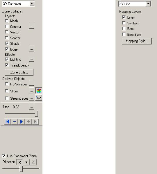
Figure 1-1. The Tecplot 360 Sidebar for a field plot (left) and a line plot (right).

The features available in the Sidebar are dependent upon the plot type.

For 3D Cartesian plots, you may add and subtract zone layers, derived objects, and effects for your plot. You may also use the Placement Plane for positioning some 3D objects (3D plots only).

For 2D Cartesian plots (not shown), you may add and subtract zone layers and some derived objects for your plot. For field plots (3D or 2D), you may animate transient data directly from the Sidebar. For Line plots you may add and subtract map layers. XY Line plots have more available map layers than polar line plots.

Plot Types

The Plot Type, combined with a frame’s dataset, active layers, and their associated attributes, define a plot. Each plot type represents one view of the data. There are five plot types available:

•3D Cartesian - 3D plots of surfaces and volumes.

•2D Cartesian - 2D plots of surfaces, where the vertical and horizontal axis are both dependent variables (i.e. x = f(A) and y = f(A), where A is another variable).

•XY Line - Line plots of independent and dependent variables on a Cartesian grid. Typically the horizontal axis (x) is the independent variable and the y-axis a dependent variable, y = f(x).

•Polar Line - Line plots of independent and dependent variables on a polar grid.

•Sketch - Create plots without data such as drawings, flow charts, and viewgraphs.

Interface

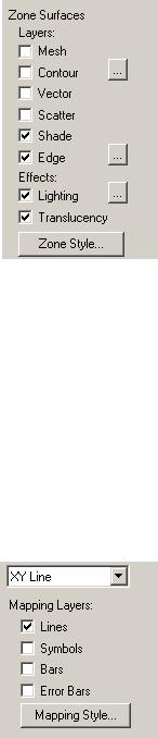
Zone Surfaces

Zone Layers

A layer is a way of representing a frame’s dataset. The complete plot is the sum of all the active layers, axes, text, geometries, and other elements added to the data plotted in the layers. The six zone layers for 2D and 3D Cartesian plot types are:

•Mesh - A grid of lines connecting the data points within each zone.

•Contour - Iso-valued lines, the region between these lines can be set to contour flooding.

•Vector - The direction and magnitude of vector quantities.

•Scatter - Symbols at the location of each data point.

•Shade - Used to tint each zone with a solid color, or to add lightsource shading to a 3D surface plot. Used in conjunction with the Lighting zone effect you may set Paneled or Gouraud shading.

Used in conjunction with the Translucency zone effect, you may create a translucent surface for your plot.

•Edge - Zone edges and creases for ordered data and creases for finite element data.

Zone Effects

For 3D Cartesian plot types, use the Sidebar to turn lighting and translucency on or off. Only shaded and flooded contour surface plot types are affected. Refer to Chapter 12: “Shade Layer” and Chapter 13: “Translucency and Lighting” for additional information.

Zone Style

Select the [Zone Style] button to launch the Zone Style dialog. The Zone Style dialog is used to customize the zone layers that you have added to your plot. Refer to the chapter for each zone layer for details on working with the Zone Style dialog.

Map Layers

A layer is a way of representing a frame’s dataset. The complete plot is the sum of all the active layers, axes, text, geometries, and other elements added to the data plotted in the layers.

The four XY Line map layers are:

•Lines - Plots a pair of variables, X and Y, as a set of line segments or a fitted curve.

•Symbols - A pair of variables, X and Y, as individual data points represented by a symbol you specify.

•Bars - A pair of variables, X and Y, as a horizontal or vertical bar chart.

•Error Bars - Allows you to add error bars to your plot.

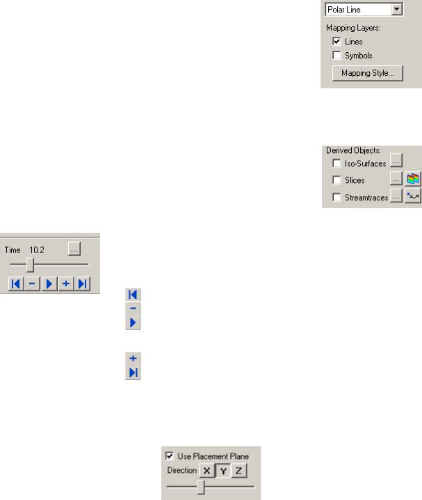
The two map layers for Polar Line are:

•Lines - A pair of variables, X and Y, as a set of line segments or a fitted curve.

•Symbols - A pair of variables, e.g. X and Y, as individual data points represented by a symbol you specify.

Select the [Mapping Style] button to launch the Mapping Style dialog. The Mapping Style dialog allows you to customize the style settings for each of the plot layers and specify the points to plot. The pages of the dialog are discussed in detail in Chapter 6: “XY and Polar Line Plots”.

Derived Objects

For Cartesian plot types (2D and 3D): Toggle-on Iso-surfaces, Slices, or Streamtraces from the Sidebar to add any or all of these elements to your plot. Their corresponding Details dialogs can be accessed via the Details [...] button. Refer to Chapter 16: “Iso-surfaces”, Chapter 14: “Slices”, or Chapter 15: “Streamtraces” for details on working with these objects.

Transient Controls

When working with transient data, simply press the Play button in the Sidebar to animate over time. The active frame will be animated from the Current Solution Time to the last time step. You may also drag the slider to change the Current Solution Time of your plot.

The Animation Controls have the following functions:

•– Jumps to the Starting Value.

•	– Jumps toward the Starting Value by one step.

• – Runs the animation as specified by the ‘Operation’ field of the Time Details dialog. The Play button becomes a Stop button while the animation is playing.

•– Jumps toward the Ending Value by one step.

• – Jumps to the Ending Value.

Use the Details [...] button to launch the Time Details dialog.

Placement Plane

When you are using certain tools to add objects to your plot, toggle-on “Use Placement Plane” in the

Sidebar to place them along a given plane (3D Plots only). Use the [X],[Y], and [Z] buttons to select the plane to use, and use the slider to reposition the Placement Plane. The Placement Plane will appear as a gray slice in your plot. The Placement Plane is available for:

Placing streamtraces (using the Add Streamtrace Tool )

Placing slices (using the Slice Tool )

Interface

Adding Contour Levels (using the Add Contour Level Tool )

Deleting Contour Levels (using the Remove Contour Level Tool )

Probing (using the Probing tool )

Snap Modes

Snap Modes allow you to place objects precisely by locking them to the nearest reference point, either on the axis grid or on the workspace paper.

•Snap to Grid - Constrain object movement to whole steps on the axis grid. This can be useful for aligning text and geometries with specific plot features.

•Snap to Paper - Constrain object movement to whole steps on the paper's ruler grid. This can be useful for positioning frames precisely for printing, or for absolute positioning of text, geometries, and other plot elements.

Details Button

The [Details] button is located immediately below the snap modes. It is context sensitive. Use this button to call up the dialog most directly applicable to your current action. When the currently selected tool is either the Selector or the Adjustor , but no objects are selected in the workspace, the [Details] button is labeled [Quick Edit]. Otherwise, the button is labeled Object Details when an object is selected and Tool Details when your mouse cursor is not in “selector” mode and an object is not selected.

Object Details

The [Object Details] button in the Sidebar calls up the dialog that most closely reflects the current state of the cursor. For example, if you select a legend and then [Object Details], the Legend dialog will open.

Tool Details

[Tool Details] calls up the dialog related to the current state of the cursor. For example, if a rotate tool is selected, [Tool Details] calls up the 3D Rotate dialog.

Redraw Buttons

The redraw buttons allow you to keep your plot up to date: [Redraw All] CTRL-D redraws all frames (SHIFT-[Redraw All] completely regenerates the workspace); [Redraw] CTRL-R redraws only the active frame.

Auto Redraw

Use Auto Redraw - When selected, the plot will be automatically redrawn, whenever style or data changes. Some users prefer to turn this option off while setting multiple style settings and then manually press the [Redraw] or [Redraw All] button on the Sidebar to see a full plot.

You can interrupt an auto-redraw at any time with a mouse click or key press.

Cache Graphics

Tecplot 360 uses OpenGL® to render plots. OpenGL provides for the ability to cache graphic instructions for rendering and can re-render the cached graphics much faster than if Tecplot 360 sends the instructions again. This is particularly true for interactive manipulation of a plot. However, this performance potential comes at the cost of using more memory. If the memory need is too high, the overall performance could be less. There are three graphics cache modes: cache all graphics, cache only lightweight graphics objects, and do not cache graphics.

When “Cache Graphics” is selected in the Sidebar, Tecplot 360 assumes there is enough memory to generate the graphics cache. Assuming this is true, Tecplot 360’s rendering performance will be optimal for interactive manipulation of plots.

When memory constraints are very limited, consider toggling-off “Cache Graphics”. If you intend to interact with the plot, also consider setting the Plot Approximation mode set to “All Frames Always Approximated”.

See Section “Graphics Cache” on page 487 for more information.

Plot Approximations

When Plot Approximation is selected and if the number of data points is above the point threshold, an approximate plot for style, data, and interactive view changes is rendered. The approximate plot is followed immediately by the full plot. This option provides for good interactive performance with the final plot always displayed in the full representation.

See Section “Plot Approximation” on page 486 for more information.

1 - 1.3 Toolbar

Each of the tools represented in the Toolbar changes the mouse mode and allows you to interactively edit your plot.

Double-click on a tool to launch the Details dialog associated with the tool.

Selector Tool

Use the Selector tool to select objects in your workspace. The selected objects can be modified using the Quick Edit dialog and (in some cases) the Selector tool itself.

The following objects can be moved (translated) using the Selector tool:

•frames

•axis grid area

•text

•geometries

•contour labels

•streamtraces

•streamtrace termination line

•legends

•3D frame axis

Interface

To select an object and open that object's attributes dialog, either double-click on any object or drag the cursor to select groups of objects (calls up Group Select dialog). Select the [OK] button, then select [Object Details].

Adjustor Tool

Use the Adjustor tool to perform any of the following modifications to your plot and data:

•Location of individual or groups of data points in the grid.

•Values of the dataset variables at a particular point.

•Length or placement of individual axes (2D Cartesian and XY Line plot types only).

•Spacing between an axis label and its associated axis (2D Cartesian and XY Line plot types only).

•Shape of a polyline.

For all other scenarios, the behavior of the Adjustor mode is identical to that of the Selector tool.

The Adjustor tool can alter your data. Be sure you want to use the Adjustor tool before dragging points in the data region.

To select multiple points - You can either SHIFT-click after selecting your initial point to select additional points, or you can draw a group select band to select the points within the band. (In line plots, you can select points from only one mapping at a time.)

Once you have selected all desired points, move the Adjustor over the selection handles of one of the points, then click-and-drag to the desired location of the first data point. The other selected points will move as a unit with respect to the chosen data point, maintaining their relative positions.

For XY Line plots, if several mappings are using the same data for one of the variables, adjusting one of the mappings will result in simultaneous adjustments to the others. You can avoid this by pressing the H or V key on your keyboard while adjusting the selected point. The H and V keys restrict the adjustment to the horizontal and vertical directions, respectively.

Group Select

The Group Select dialog is opened when you select a group of objects with the Selector or Adjustor tool.

The Group Select dialog allows you to specify the following object types (if the selection rectangle does not include a specific object, its associated check box is inactive):

•Text

•Geometries

•Frames

•Zones or Mappings

•Axis Grid Area

•Contour Labels

•Streamtraces

The Group Select dialog offers the following attribute filters:

• Geoms of Type - Choose geometries of a particular type from the drop-down menu.

•Geoms with Line Pattern - Choose all geometries having a particular line pattern.

•Text with Font - Choose all text displayed in a particular font.

•Objects with Color - Choose all objects of a particular color. You choose the appropriate color from the Select Color dialog.

Zoom Tool

Zoom into or away from the plot.

When a mouse-click occurs (without dragging), the zooming is centered at the location of your click.

There are two zoom modes: plot zooming and paper zooming.

For plot zooming - drag the magnifying glass cursor to draw a box around the region that you want to fit into the frame. The box may be larger than the frame. Making the box larger than the frame zooms away from the plot. The region within the view box will be resized to fit into the frame.

If Snap to Grid (located in the Sidebar) is selected, you cannot make the zoom box larger than the grid area.

To return to the previous view, choose “Last” from the View menu (CTRL-L). To restore the original 2D view, choose” Fit to Full Size (CTRL-F)”.

The results of plot zooming for the 2D plot type are dependent upon the axis mode selected in the Axis Details dialog (accessed via the Plot menu):

•2D Independent Axis Mode - Allows the selected region to expand to exactly fit in the frame. The axes are rescaled independently to fit the zoom box.

•2D Dependent Axis Mode - In dependent mode, the axes are not fit perfectly to the zoom box. The longest dimension from the zoom box is applied to an associated axis, and the other axis is resized according to the dependency relation.

For paper zooming - SHIFT-drag the magnifying glass cursor to draw a box about the region that you want to magnify. The plot is resized so that the longest dimension of the zoom box fits into the workspace. You can fit one or all frames to the workspace by using the “Fit Selected Frames to Workspace” or “Fit All Frames to Workspace” options from the View>Workspace menu. To return to the default paper view, choose “Fit Paper to Workspace” from the View>Workspace menu.

Clicking anywhere in your plot while the zoom tool is active will center the zoom around your click. Alternatively, CTRL-click centers the plot on the point that was clicked and zooms out.

Use the center mouse button and drag (or hold down the rollerball and drag) to interactively zoom into or out of the plot.

Translate Tool

Use the Translate/Magnify tool to translate or magnify data within a frame or the paper within the workspace.

Interface

While in Translate/Magnify mode, drag the cursor to move the data with respect to the frame, or SHIFTdrag to move the paper with respect to the workspace.

Use the right mouse button to interactively translate objects. You can rescale your image by pressing “+” to magnify, “-” to shrink. If you are SHIFT-dragging to move the paper, the rescale buttons “+” and “-” will magnify or shrink the paper, as long as you have the mouse button depressed.

Three-dimensional Rotation

There are six 3D rotation mouse modes:

Spherical - Drag the mouse horizontally to rotate about the Z-axis; drag the mouse vertically to control the tilt of the Z-axis.

Rollerball - Drag the mouse in a direction to move with respect to the current orientation on the screen. In this mode, your mouse acts much like a rollerball.

Twist - Drag the mouse clockwise around the image to rotate the image clockwise. Drag the mouse counterclockwise around the image to rotate the image counterclockwise.

X-axis - Drag the mouse to rotate the image about the X-axis.

Y-axis - Drag the mouse to rotate the image about the Y-axis.

Z-axis - Drag the mouse to rotate the image about the Z-axis.

Once you have selected a rotation mouse mode, you can quickly switch to any of the others using the following keyboard shortcuts:

	Drag	Rotate about the defined rotation origin with your current Rotate tool.

	ALT-drag	Rotate about the viewer position using your current Rotate tool.

	Middle-click-and-drag/ALT-	Smooth zoom in and out of the data.
	right click-and-drag	Smooth zoom in and out of the data.
	right click-and-drag

	Right-click-and-drag	Translate the data.

		This option can be used without first selecting a rotation mouse mode. Simply
	CTRL-right-click-and-drag	hover over your intended point of origin, and then CTRL-right-click-and-drag
		to translate the image.

	C	Move rotation origin to probed point, ignoring zones.

		Move rotation origin to probed point of data.
	O	This shortcut can be used without first selecting a rotation mouse mode.
	O	Simply hover over your intended point of origin, type O, and then CTRL-

		right-click-and-drag to rotate the image.

	R	Switch to Rollerball rotation.

	S	Switch to Spherical rotation.

	T	Switch to Twist rotation.

	X	Switch to X-axis rotation.

	Y	Switch to Y-axis rotation.

	Z	Switch to Z-axis rotation.

Slice Tool

Use the Slicing tool to add a slice interactively by clicking anywhere in your plot. You can also use this tool to control your slice(s) interactively.

The following keyboard/mouse options are available when the Slice tool is active:

		Primary Slices, Start End Slices Active - Turn on intermediate slices (if not
	+	already active) and adds a slice.
	+	Primary Slices active [ONLY] - Turns on Start/End Slices and adds a slice.

		Start/End Slices active [ONLY] - Turns on Start/End Slices and adds a slice.

		Primary Slices, Start End Slices Active - Removes start and end slices.
	-	Primary Slices active [ONLY] - Removes the primary slice.
		Start/End Slices active [ONLY] - Removes the Start and End Slices.

	Click/Drag	Updates the position of the primary slice (if active). If only start and end slices
	Click/Drag	are visible, click updates the position of the starting slice.


	ALT-click/ALT-drag	Determine the XYZ-location by ignoring zones and looking only at derived
	ALT-click/ALT-drag	volume objects (streamtraces, slices, iso-surfaces).
		volume objects (streamtraces, slices, iso-surfaces).

	SHIFT-click	Switches from one Primary slice to Start/End Slices by adding a slice.

	SHIFT-drag	Move the start or end slice (whichever is closest to the initial click location).
	SHIFT-drag	Show Start/End Slices is activated, if necessary.
		Show Start/End Slices is activated, if necessary.

	I, J, K (ordered zones only)	Switch to slicing constant I, J, or K-planes respectively.

	X, Y, Z	Switch to slicing constant X, Y, or Z-planes respectively.

	1-8	Numbers one through eight switch to the corresponding slice group.

Interface

Add Streamtrace

Select the Add Streamtrace tool to add a streamtrace interactively by clicking anywhere in your plot. Select the number of streamtraces to include with each click (rake) using 1-9 on the keyboard.

Keyboard Shortcuts

DSwitch to streamrods RSwitch to streamribbons SSwitch to surface lines VSwitch to volume lines

1-9Change the number of streamtraces to be added when placing a rake of streamtraces

SHIFT - Draws a rake on concave 3D volume surfaces. These rakes are normally not drawn, as they occur outside of the data

Refer to Chapter 15: “Streamtraces” for more information.

Streamtrace Termination Line

Select the Add Streamtrace Termination Line tool to add a streamtrace termination line interactively.

To draw a Streamtrace Termination Line:

•Move the cursor into the data region.

•Click once at the desired starting point for the line.

•Click again at each desired break point.

•When the polyline is complete, double-click on the last point of the polyline, or press ESC on your keyboard.

•The drawn polyline ends any streamtraces that pass through it.

Add Contour Level

Select the Add Contour Level tool to add a contour level by clicking anywhere in the active data region. A new contour level, passing through the specified location, is calculated and drawn.

The following keyboard and mouse shortcuts are related to the Add Contour Level tool.

ALT-click	Place a contour line by probing on a streamtrace, slice, or iso-surface.

Click	Place a contour line.

CTRL-Click	Replace the nearest contour line with a new line.

Drag	Move the new contour line.

-	Switch to the Delete Contour Level tool.

Delete Contour Level

Select the Delete Contour Level tool to delete a contour level by clicking anywhere in the active data region. The contour line nearest the specified location is deleted.

Use the “+” key to switch to the Add Contour Level tool and the “-” key to switch back to the Delete Contour Level tool.

Add Contour Labels

Select the Add Contour Label tool to switch to the Contour Label mode, enabling you to add a contour label by clicking anywhere in the active data region.

A contour label is added to the plot at the specified location; its level or value information is taken from the nearest contour line. This allows you to place labels at a slight offset from the lines they label.

The Contour type must be lines or lines and flood in order for this tool to be active. You can set the contour type on the Contour page of the Zone Style dialog.

Probe Tool

Select the Probe At Tool to probe for values of the dataset's variables at a particular point.

To obtain interpolated values of the dataset variables at the specified location, click at any point in the data region.

To obtain exact values for the data point nearest the specified location, CTRL-click at the desired location.

For XY plots, when you move into the axis grid area, the cursor cross hair is augmented by a vertical or horizontal line, depending on whether you are probing along the X-axis or the Y-axis. You can change the axis to probe simply by pressing X to probe the X-axis or Y to probe the Y-axis.

Insert Text

Select the Add Text tool to add text to any frame.

Insert Geometries

Use the corresponding geometry buttons in the Toolbar to insert geometries into your plot.

Polylines

Squares

Rectangles

Circle

Ellipse

Interface

Create New Frame

Select the Create Frame tool to create a new frame.

To add a frame:

•Click once in the workspace to anchor one corner of the frame.

•Drag the diagonal corner until the frame is the desired size and shape.

If you have data loaded before you create a new frame, you can attach the existing dataset to the new frame by changing the plot type.

Extract Discrete Points

Select the Extract Discrete Points tool to extract selected points to a data file or a new zone.

To select points:

•Click your left-hand mouse button at each location where you would like to extract a point.

•To end extraction, either double-click on the last point, or right click, or press the ESC key.

•The Extract Data Points dialog appears; use it to specify how many points to extract and how to save the data.

Extract Points along Polyline

Select the Extract Line tool to extract points along a specified polyline to a data file or a new zone.

To select points:

•Click your left-hand mouse button at each location where you would like to extract a point.

•To end extraction, either double-click on the last point, or right click, or press the ESC key.

•The Extract Data Points dialog appears; use it to specify how many points to extract and how to save the data.

Create Rectangular Zone

Select the Create Rectangular Zone tool to add 2D rectangular zones to the active dataset.

To create a rectangular zone:

•Click once in the active data region to anchor one corner of the zone.

•Drag the diagonal corner until the zone is the desired size and shape. The new zone created is IJ-ordered.

To specify the maximum I-index and J-index, use the Create Rectangular Zone dialog (accessed via

Data>Create Zone).

The active frame must have a dataset attached to it in order for this tool to be active. This tool is available in 2D plots only.

Create Circular Zone

Select the Create Circular Zone tool to add new 2D circular zones to the active dataset.

To create a circular zone:

•Click once in the active data region to specify the center of the zone.

•Drag until the zone has the desired radius. The new zone created is IJ-ordered.

To specify the maximum I-index and J-index, use the Create Circular Zone dialog (accessed via

Data>Create Zone).

The active frame must have a dataset attached to it in order for the Create Circular Zone tool to be active. This tool is available in 2D plots only.

1 - 1.4 Status Line

The status line appears along the bottom of the Tecplot 360 window to give “hover help”, as well as a progress bar and information when Tecplot 360 computes calculations. The hover help appears when you move the pointer over a tool in the Toolbar, a button or item in the sidebar, or a menu item, and gives a description of the control.

A progress bar and information about the calculation Tecplot 360 is completing appears in the status line during lengthy calculations or other longer operations.

1 - 1.5 Tecplot 360 Workspace

In the Tecplot 360 workspace, you can create sketches and plots. You can create each sketch or plot within a window called a frame. Each visible measure of the workspace is called a page. The current state of the workspace, including the sizing and positioning of frames, the number and contents of pages, the location of the data files used by each frame, and all current attributes for all frames, makes up a layout. By default, the workspace displays a representation of where the paper plots are drawn, as well as a reference grid and rulers. The frame most recently selected is called the active frame.

You can include multiple pages in your layout. To create a new page, modify pages or move between them, use the Quick Macro Panel. See Section 28 - 2.1 “Quick Macro Panel” for more information about the panel.

Interface

1 - 1.6 Quick Edit

The map and zone layer controls affecting how the individual layers are drawn can be altered using controls on the Sidebar. You can also control many of these attributes using the Quick Edit dialog.

The Quick Edit dialog is accessed via the [Quick Edit] button located at the bottom of the Sidebar when the mouse-mode is a standard arrow (i.e. you are using either the Selector Tool or Adjustor Tool). If you are in a different mouse mode, or you have selected a Text or Geometry object, the Object Details or Tool Details will be launched in lieu of the Quick Edit dialog.

To use the Quick Edit dialog, select one or more objects in the workspace, then select the appropriate button in the dialog to change the attributes of the selected object(s). The functionality of each button is described in the following sections.

Mesh

This area of the Quick Edit dialog controls whether the mesh is displayed for selected zones, and if so, using which types of mesh. The following options are available:

•Y - Show the mesh for the selected zones. The first time you turn on the Mesh layer by either the Quick Edit dialog or the Zone Style dialog, a dialog appears asking if you wish it activated. Select [Yes] to confirm turning on the layer.

•N - Turn off the mesh for the selected zones.

• Wire Frame - Mesh lines are drawn underlying all other field layers (i.e., Contour, Vector, Scatter, Shade); hidden lines are not removed.

• Overlay - Mesh lines are drawn above all other field plot layers except vectors and scatter symbols.

• Hidden - Similar to Overlay, except that in the 3D Cartesian, plot type hidden lines are removed from behind the mesh. In essence, the cells of the mesh are opaque. Surfaces and lines that are hidden behind another surface are removed from the plot.

Contour

This area of the Quick Edit dialog controls whether contours are displayed for selected zones, and if so, using which plot type. The following options are available:

•Y - Show the contours for the selected zones. The first time you turn on the Contour layer by either the Quick Edit dialog or the Zone Style dialog, a dialog appears asking if you wish it activated. Select [Yes] to confirm turning on the layer.

•N - Turn off the contour for the selected zones.

• Lines - Plots contour lines. If you choose this plot type, you can use the Cont Color attribute to specify Multi-Color to make the line color vary with the contour-variable value.

• Flood - Flood the area between adjacent contour lines with a color according to the value of the contour variable, number of contour levels, and the Color Map.

• Both Lines and Flood - Contour lines are drawn with color flooding between them.

• Average Cell - Each cell or element is flooded with one solid color based upon the average value of the contour variable at the data points of the cell or element.

• Primary Value - Each cell or element is flooded with one solid color based upon the primary cell value.

Vector

This area of the Quick Edit dialog controls whether vectors are displayed for selected zones, and if so, using which plot type. The following options are available:

•Y - Show the vectors for the selected zones. The first time you turn on the Vector layer by either the Quick Edit dialog or the Zone Style dialog, a dialog appears asking if you wish it activated. Select [Yes] to confirm turning on the layer.

•N - Turn off the vectors for the selected zones.

• Tail at Point - Display regular vectors – a simple stick vector with length proportional to the local magnitude. The tail of the vector is positioned at the data point.

+ 568 hidden pages

Tecplot 360 2011 R2 User Guide

Table of Contents

Introduction

1 - 1 Interface

1 - 1.1 Menubar

1 - 1.2 Sidebar

1 - 1.3 Toolbar

1 - 1.4 Status Line

1 - 1.5 Tecplot 360 Workspace

1 - 1.6 Quick Edit