Tecplot 360 2011 R2 User Guide

Tecplot, Inc.

Bellevue, WA

2011

User’s Manual

Release 2

COPYRIGHT NOTICE

TM

User’s Manual is f or use with Tecplot 360

Tecplot 360

Copyright © 1988-2011 Tecplot, Inc. All rights reserved worldwide. Except for personal use, this manual may not be reproduced, transmitted, transcribed, stored in a retrieval system, or translated in any form, in whole or in part, without the express written
permission of Tecplot, Inc., 3535 Factoria Blvd, Ste. 550; Bellevue, WA 98006 U.S.A.

The software discussed in this documentation and the documentation itself are furnished under license for utilization and duplication
information only. It is subject to change without notice. It should not be interpreted as a commitment by Tecplot, Inc. Tecplot, Inc. assumes no liability or responsibility for documentation errors or inaccuracies.

Tec plo t, I nc.
Post Office Box 52708
Bellevue, WA 98015-2708 U.S.A.
Tel:[phone] (within the U.S. or Canada), 00 1 [phone] (internationally)
email: [e-mail], [e-mail]
Questions, comments or concerns regarding this document: [e-mail]
For more information, visit http://www.tecplot.com

THIRD PARTY SOFTWARE COPYRIGHT NOTICES

LAPACK 1992-2007 LAPACK Copyright © 1992-2007 the University of Tennessee. All rights reserved. Redistribution and use in source and binary forms, with or without modification, are permitted provided that the following conditions are met: Redistribu­tions of source code must retain the above copyright notice, this list of conditions and the following disclaimer. Redistributions in binary form must reproduce the above copyright notice, this list of conditions and the following disclaimer listed in this cense in
the documentation and/or other materials provided with the distribution. Neither the name of the copyright holders nor the names of its contributors may be used to endorse or promote products derived from this software without pecific prior written per­mission. THIS SOFTWARE IS PROVIDED BY THE COPYRIGHT HOLDERS AND CONTRIBUTORS "AS IS" AND ANY EXPRESS OR IMPLIED WARRANTIES, INCLUDING, BUT NOT LIMITED TO, THE IMPLIED WARRANTIES OF MERCHANTABILITY
AND FITNESS FOR A PARTICULAR PURPOSE ARE DISCLAIMED. IN NO EVENT SHALL THE COPYRIGHT OWNER OR CONTRIBUTORS BE LIABLE FOR ANY DIRECT, INDIRECT, INCIDENTAL, SPECIAL, EXEMPLARY, OR CONSEQUENTIAL
DAMAGES (INCLUDING, BUT NOT LIMITED TO, PROCUREMENT OF SUBSTITUTE GOODS OR SERVICES; LOSS OF USE, DATA, OR PROFITS; OR BUSINESS INTERRUPTION) HOWEVER CAUSED AND ON ANY THEORY OF LIABILITY,
WHETHER IN CONTRACT, STRICT LIABILITY, OR TORT (INCLUDING NEGLIGENCE OR OTHERWISE) ARISING IN ANY WAY OUT OF THE USE OF THIS SOFTWARE, EVEN IF ADVISED OF THE POSSIBILITY OF SUCH DAMAGE. The University
of Tennessee. All Rights Reserved. SciPy 2001-2009 Enthought. Inc. All Rights Reserved. NumPy 2005 NumPy Developers. All Rights Reserved. VisTools and VdmTools 1992-2009 Visual Kinematics, Inc. All Rights Reserved. NCSA HDF & HDF5 (Hierarchical
Data Format) Software Library and Utilities Contributors: National Center for Supercomputing Applications (NCSA) at the University of Illinois, Fortner Software, Unidata Program Center (netCDF), The Independent JPEG Group (JPEG), Jean-loup Gailly
and Mark Adler (gzip), and Digital Equipment Corporation (DEC). Conditions of Redistribution: 1. Redistributions of source code must retain the above copyright notice, this list of conditions, and the following disclaimer. 2. Redistributions in binary form
must reproduce the above copyright notice, this list of conditions, and the following disclaimer in the documentation and/or materials provided with the distribution. 3. In addition, redistributions of modified forms of the source or binary code must carry
prominent notices stating that the original code was changed and the date of the change. 4. All publications or advertising materials mentioning features or use of this software are asked, but not required, to acknowledge that it was developed by The HDF
Group and by the National Center for Supercomputing Applications at the University of Illinois at Urbana-Champaign and credit the contributors. 5. Neither the name of The HDF Group, the name of the University, nor the name of any Contributor may be
used to endorse or promote products derived from this software without specific prior written permission from the University, THG, or the Contributor, respectively. DISCLAIMER: THIS SOFTWARE IS PROVIDED BY THE HDF GROUP (THG) AND THE
CONTRIBUTORS "AS IS" WITH NO WARRANTY OF ANY KIND, EITHER EXPRESSED OR IMPLIED. In no event shall THG or the Contributors be liable for any damages suffered by the users arising out of the use of this software, even if advised of the pos­sibility of such damage. Copyright © 1998-2006 The Board of Trustees of the University of Illinois, Copyright © 2006-2008 The HDF Group (THG). All Rights Reserved. PNG Reference Library Copyright © 1995, 1996 Guy Eric Schalnat, Gro up 42, Inc., Copy­right © 1996, 1997 Andreas Dilger, Copyright © 1998, 1999 Glenn Randers-Pehrson. All Rights Reserved. Tcl 1989-1994 The Regents of the Universi ty of California. Copyright © 1994 The Australian National University. Copyright © 1994-1998 Sun
Microsystems, Inc. Copyright © 1998-1999 Scriptics Corporation. All Rights Reserved. bmptopnm 1992 David W. Sanderson. All Rights Reserved. Netpbm 1988 Jef Poskanzer . All Rights Reserved. Mesa 1999-2003 Brian Paul. All Rights Reserved. W3C IPR
1995-1998 World Wide Web Consortium, (Massachusetts Institute of Technology, Institut National de Recherche en Informatique et en Automatique, Keio University). All Rights Reserved. Ppmtopict 1990 Ken Yap. All Rights Reserved. JPEG 1991-1998 Thomas
G. Lane. All Rights Reserved. Dirent API f or Microsoft Visual Studio (dirent.h) 2006-2006 Copyright © 2006 Toni Ronkko. Permission is hereby granted, free of charge, to any person obtaining a copy of this software and associated documentation files (the
``Software''), to deal in the Software without restriction, including without limitation the rights to use, copy, modify, merge, publish, distribute, sublicense, and/or sell copies of the Software, and to permit persons to whom the Software is furnished to do so.
Toni Ronkko. All Rights Reserved. ICU 1995-2009 Copyright © 1995-2009 International Business Machines Corporation and others. All rights reserved. Permission is hereby granted, free of charge, to any person obtaining a copy of this software and associated
documentation files (the "Software"), to deal in the Software without restriction, including without limitation the rights to use, copy, modify, merge, publish, distribute, and/or sell copies of the Software, and to permit persons to whom the Software is furnished
to do so, provided that the above copyri ght notice(s) and this permission notice appear in all copies of the Software and that both the above copyright notice(s) and this permission notice appear in supporting documentation. International Business Machines
Corporation and others. All Rights Reserved. QsLog 2010 Copyright © 2010, Razvan Petru. All rights reserved. QsLog Copyright (c) 2010, Razvan Petru. All rights reserved. Redist ribution and use in source and binary forms, with or without modification, are
permitted provided that the following onditions are met: Redistributions of source code must retain the above copyright noti ce, this list of conditions and the following disclaimer. Redistributions in binary form must reproduce the above copyright notice, this
list of conditions and the following disclaimer in the documentation and/or other materials provided with the distribution. The name of the contributors may not be used to endorse or promote products derived from this software without specific prior written
permission. THIS SOFTWARE IS PROVIDED BY THE COPYRIGHT HOLDERS AND CONTRIBUTORS "AS IS" AND ANY EXPRESS OR IMPLIED WARRANTIES, INCLUDING, BUT NOT LIMITED TO, THE IMPLIED WARRANTIES OF MERCHANTABIL­ITY AND FITNESS FOR A PARTICULAR PURPOSE ARE DISCLAIMED. IN NO EVENT SHALL THE COPYRIGHT HOLDER OR CONTRIBUTORS BE LIABLE FOR A
TIAL DAMAGES (INCLUDING, BUT NOT LIMITED TO, PROCUREMENT OF SUBSTITUTE GOODS OR SERVICES; LOSS OF USE, DATA, OR PROFITS; OR BUSINESS INTERRUPTION) HOWEVER CAUSED AND ON ANY THEORY OF LIABILITY,
WHETHER IN CONTRACT, STRICT LIABILITY, OR TORT (INCLUDING NEGLIGENCE OR OTHERWISE) ARISING IN ANY WAY OUT OF THE USE OF THIS SOFTWARE, EVEN IF ADVISED OF THE POSSIBILITY OF SUCH DAMAGE. Razvan Petru.
All Rights Reserved. VTK 1993-2008 Copyright © 1993-2008 Ken Martin, Will Schroeder, Bill Lorenson. All rights reserved. Redistribution and use in source and binary forms, with or without modification, are permitted provided that the following conditions
are met: Redistributions of source code must retain the above copyright notice, this list of conditions and the following disclaimer. Redistributions in binary form must reproduce the above copyright notice, this list of conditions and the following disclaimer
in the documentation and/or other materials provided with the distribution. Neither name of Ken Martin, Will Schroeder, or Bill Lorensen nor the names of any contributors may be used to endorse or promote products derived from this software without spe­cific prior written permission. THIS SOFTWARE IS PROVIDED BY THE COPYRIGHT HOLDERS AND CONTRIBUTORS ``AS IS'' AND ANY EXPRESS OR IMPLIED WARRANTIES, INCLUDING, BUT NOT LIMITED TO, THE IMPLIED WARRANTIES OF
MERCHANTABILITY AND FITNESS FOR A PARTICULAR PURPOSE ARE DISCLAIMED. IN NO EVENT SHALL THE AUTHORS OR CONTRIBUTORS BE LIABLE FOR ANY DIRECT, INDIRECT, INCIDENTAL, SPECIAL, EXEMPLARY, OR CONSE­QUENTIAL DAMAGES (INCLUDING, BUT NOT LIMITED TO, PROCUREMENT OF SUBSTITUTE GOODS OR SERVICES; LOSS OF USE, DATA, OR PROFITS; OR BUSINESS INTERRUPTION) HOWEVER CAUSED AND ON ANY THEORY OF LIABIL­ITY, WHETHER IN CONTRACT, STRICT LIABILITY, OR TORT (INCLUDING NEGLIGENCE OR OTHERWISE) ARISING IN ANY WAY OUT OF THE USE OF THIS SOFTWARE, EVEN IF ADVISED OF THE POSSIBILITY OF SUCH DAMAGE. Ken Martin,
Will Schroeder, Bill Lorenson. All Rights Reserved.

TRADEMARKS

®

Tec pl ot,

Tecplot 360,TM the Tecplot 360 logo, Preplot,TM Enjoy the View,TM Master the View,TM and FramerTM are registered trademarks or trademarks of Tecplot, Inc. in the United States and other countries.

3D Systems is a registered trademark or trademark of 3D Systems Corporation in the U.S. and/or other countries. Macintosh OS is a registered trademark or trademark of Apple, Incorporated in the U.S. and/or other countries. Reflection-X is a registered trade­mark or trademark of Attachmate Corporation in the U.S. and/or other countries. EnSight is a registered trademark or trademark of Computation Engineering Internation (CEI), Incorporated in the U.S. and/or other countries. EDEM is a registered trademark
or trademark of DEM Solutions Ltd in the U.S. and/or other countries. Exceed 3D, Hummingbird, and Exceed are registered trademarks or trademarks of Hummingbird Limited in the U.S. and/or other countries. Konqueror is a registered trademark or trade­mark of KDE e.V. in the U.S. and/or other countries. VIP and VDB are registered trademarks or trademarks of Halliburton in the U.S. and/or other countries. ECLIPSE FrontSim is a registered trademark or trademark of Schlumberger Information Solutions
(SIS) in the U.S. and/or other countries. Debian is a registere d trademark or trademark of Software in the Public Interest, Incorporated in the U.S. and/or other countries. X3D is a registered trademark or trade mark of Web3D Consortium in the U.S. and/or other
countries. X Window System is a registered trademark or trademark of X Consortium, Incorporated in the U.S. and/or other countries. ANSYS, Fluent and any and all ANSYS, Inc. brand, product, servic e and feature names, logos and slogans are registered
trademarks or trademarks of ANSYS Incorporated or its subsidiaries in the U.S. and/or other countries. PAM-CRASH is a registered trademark or trademark of ESI Gr oup in the U.S. and/or other countries. LS-DYNA is a registered trademark or trademark of
Livermore Software Technology Coroporation in the U.S. and/or other countries. MSC/NASTRAN is a registered trademark or trademark of MSC.Software Corporation in the U.S. and/or other countries. NASTRAN is a registered trademark or trademark of
National Aeronautics Space Administration in the U.S. and/or other countries. 3DSL is a registered trademark or trademark of StreamSim Technologies, Incorporated in the U.S. and/or other countries. SDRC/IDEAS Universal is a registered trademark or trade­mark of UGS PLM Solutions Incorporated or its subsidiaries in the U.S. and/or other countries. St ar-CCM+ is a registered trademark or trademark of CD-adapco in the U.S. and/or other countries. Reprise License Manager is a registered trademark or trade­mark of Reprise Software, Inc. in the U.S. and/or other countries. Python is a registered trademark or trademark of Python Software Foundation in the U.S. and/or other countries. Abaqus, the 3DS logo, SIMULIA and CATIA are registered trademarks or
trademarks of Dassault Systèmes or its subsidiaries in the U.S. and/or other countries. The Abaqus runtime libraries are a product of Dassault Systèmes Simulia Corp., Providence, RI, USA. © Dassault Systèmes, 2007 FLOW-3D is a registered trademark or
trademark of Flow Science, Incorpo rated in the U.S. and/or other countries. Adobe, Flash, Flash Pl ayer, Premier and PostScript are registered trademarks or trademarks of Adobe Systems, Incorporated in the U.S. and/or other countries. AutoCAD and DXF are
registered trademarks or trademarks of Autodesk, Incorporated in the U.S. and/or other countries. Ubuntu is a registered trademark or trademark of Canonical Limited in the U.S. and/or other countries. HP, LaserJet and PaintJet are registered trademarks or
trademarks of Hewlett-Packard Development Company, Limited Partnership in the U.S. and/or other countries. I BM, RS/6000 and AIX are registered trademarks or trademarks of International Business Machines Corporation in the U.S. and/or other countries.
Helvetica Font Family and Times Font Family are regist ered trademarks or trademarks of Linotype GmbH in the U.S. and/or other countries. Linux is a registered trademark or trademark of Linus Torvalds in the U.S. and/or other countries. ActiveX, Excel,
Microsoft, Visual C++, Visual Studio, Windows, Windows Metafile, Windows XP, Windows Vista, Windows 2000 and PowerPoint are registered trademarks or trademarks of Microsoft Corporation in the U.S. and/or other countries. Firefox is a registered trade­mark or trademark of The Mozilla Foundation in the U.S. and/or other countries. Netscape is a registered trademark or trademark of Netscape Communications Corporation in the U.S. and/or other countries. SUSE is a registered trademark or trademark of
Novell, Incorporated in the U.S. and/or other countries. Red Hat is a registered trademark or trademark of Red Hat, Incorporated in the U.S. and/or other countries. SPARC is a registered trademark or trademark of SPARC International, Incorporated in the
U.S. and/or other countries. Products bearing SPARC trademarks are based on an architecture developed by Sun Microsystems, Inc. Solaris, Sun and SunRaster are registered trademarks or trademarks of Sun MicroSystems, Incorporated in the U.S. and/or
other countries. Courier is a registered trademark or trademark of Monotype Imaging Incorporated in the U.S. and/or other countries. UNIX and Motif are registered trademarks or trademarks of The Open Group in the U.S. and/or other countries. Qt is a reg­istered trademark or trademark of Trolltech in the U.S. and/or other c ountries. Zlib is a registered trademark or trademark of Jean-loup Gailly and Mark Adler in the U.S. and/or other countries. OpenGL is a registered trademark or trademark of Silicon Graph­ics, Incorporated in the U.S. and/or other countries. JPEG is a registered trademark or trademark of Thomas G. Lane in the U.S. and/or other countries. SENSOR is a registered trademark or trademark of Coats Engineering in the U.S. and/or other countries.
SENSOR is licensed and distributed only by Coats Engineering and by JOA Oil and Gas, a world-wide authorized reseller. MySQL is a registered trademark or trademark of Oracle in the U.S. and/or other countries. MySQL is a trademark of Oracle Corpora­tion and/or its affiliates. All other product names mentioned herein are trademarks or registered trademarks of their respective owners.

NOTICE TO U.S. GOVERNMENT END-USERS

Use, duplication, or disclosure by the U.S. Government is subject to restrictions as set forth in subparagraphs (a) through (d) of the Commercial Computer-Restricted Rights clause at FAR 52.227-19 when applicable, or in subparagraph (c)(1)(ii) of the Rights in
Technical Data and Computer Software clause at DFARS 252.227-7013, and/or in similar or successor clauses in the DOD or NASA FAR Supplement. Contractor/manufacturer is Tecplot, Inc., 3535 Factoria Blvd, Ste. 550; Bellevue, WA 98006 U.S.A.

11-360-01-2

Rev 4/2011

TM

Version 2011 R2.

only

according to the license terms. The copyright for the software is held by Tecplot, Inc. Documentation is provided for

NY DIRECT, INDIRECT, INCIDENTAL, SPECIAL, EXEMPLARY, OR CONSEQUEN-

Table of Contents

Introduction to Tecplot 360

1 Introduction .................................................................................................... 13

Interface

Getting Help.......................................................................................................................35

...............................................................................................................................14

2 Using the Workspace ............................................................................... 37

Data Hierarchy

Interface Coordinate Systems ......................................................................................39

Frames..................................................................................................................................40

Workspace Management Options Menu.................................................................. 49

View Modification ...........................................................................................................51

Edit Menu ...........................................................................................................................54

.................................................................................................................. 37

3 Data Structure .............................................................................................. 57

Connectivity List

Ordered Data..................................................................................................................... 58

Finite Element Data.........................................................................................................61

Variable Location (Cell-centered or Nodal)............................................................. 62

Face Neighbors..................................................................................................................63

Working with Unorganized Datasets........................................................................ 63

.............................................................................................................. 57

3

Loading Your Data

4 Data Loaders .................................................................................................. 69

CGNS Loader

DEM Loader.......................................................................................................................74

DXF Loader ........................................................................................................................ 75

EnSight Loader.................................................................................................................. 76

Excel Loader.......................................................................................................................77

FEA Loader ........................................................................................................................81

FLOW-3D Loader.............................................................................................................88

FLUENT Loader ...............................................................................................................92

General Text Loader ........................................................................................................ 97

HDF Loader .....................................................................................................................106

HDF5 Loader ...................................................................................................................107

Kiva Loader......................................................................................................................109

PLOT3D Loader..............................................................................................................110

PLY Loader....................................................................................................................... 115

Tecplot-Format Loader.................................................................................................116

Text Spreadsheet Loader..............................................................................................123

Overwriting Data Files .................................................................................................124

.................................................................................................................... 70

Creating Plots

5Creating Plots .............................................................................................. 129

Creating Plots

Data Journaling...............................................................................................................130

Data Sharing ....................................................................................................................130

Dataset Information....................................................................................................... 131

Select Color.......................................................................................................................137

.................................................................................................................. 129

6 XY and Polar Line Plots ......................................................................... 143

Mapping Style and Creation

Line Map Layer...............................................................................................................149

Symbols Map Layer....................................................................................................... 163

XY Line Error Bars.........................................................................................................165

XY Line Bar Charts ........................................................................................................ 167

I, J, and K-indices ...........................................................................................................167

Line Legend...................................................................................................................... 168

Polar Drawing Options ................................................................................................170

......................................................................................144

7 Field Plots ....................................................................................................... 173

Field Plot Modification - Zone Style Dialog

..........................................................174

4

Time Aware ...................................................................................................................... 179

Data Point and Cell Labels..........................................................................................181

Three-dimensional Plot Control................................................................................182

8 Mesh Layer and Edge Layer ............................................................. 189

Mesh Layer

Edge Layer........................................................................................................................191

....................................................................................................................... 189

9 Contour Layer .............................................................................................. 193

Contour Layer Modification

Contour Details Dialog.................................................................................................195

Extract Contour Lines...................................................................................................204

.......................................................................................194

10 Vector Layer .................................................................................................. 207

Vec tor Variables

Vector Plot Modification ..............................................................................................208

Vec tor Arrowheads ........................................................................................................210

Vector Length................................................................................................................... 211

Reference Vectors ...........................................................................................................212

..............................................................................................................207

11 Scatter Layer ................................................................................................ 215

Scatter Plot Modification

Scatter Size/Font .............................................................................................................217

Reference Scatter Symbols...........................................................................................218

Scatter Legends ............................................................................................................... 219

.............................................................................................215

12 Shade Layer .................................................................................................. 221

Shade Layer Modification

...........................................................................................221

13 Translucency and Lighting ................................................................. 223

Transluc ency

Lighting Effects...............................................................................................................224

Three-dimensional Light Source............................................................................... 225

.................................................................................................................... 223

14 Slices .................................................................................................................. 227

Interactively Created Slices

Slices Extracted Directly to Zones ............................................................................232

.........................................................................................228

15 Streamtraces ................................................................................................ 235

Streamtrace Details dialog

Streamtrace Animation ................................................................................................245

Surface Streamtraces on No-slip Boundaries........................................................245

..........................................................................................236

5

Streamtrace Extraction as Zones ...............................................................................245

Streamtrace Errors .........................................................................................................245

16 Iso-surfaces .................................................................................................. 247

Iso-Surface Groups

Iso-Surface Definition ...................................................................................................248

Iso-Surface Style .............................................................................................................249

Iso-Surface Animation..................................................................................................249

Iso-Surface Extraction...................................................................................................250

........................................................................................................247

17 Axes .................................................................................................................... 251

Axis Display

Axis Variable Assignment........................................................................................... 251

Axis Range Options for XY Line, 2D, and 3D Cartesian Coordinates..........252

Axis Range Options for Polar Coordinates ........................................................... 254

Axis Grid Options..........................................................................................................256

Tick Mark Options.........................................................................................................258

Tick Mark Label Options.............................................................................................259

Axis Title Options .......................................................................................................... 263

Axis Line Options ..........................................................................................................263

Grid Area Options ......................................................................................................... 266

Time/Date Format Options.........................................................................................266

..................................................................................................................... 251

18 Text, Geometries, and Images ...................................................... 271

......................................................................................................................................271

Tex t

Geometries........................................................................................................................282

Images................................................................................................................................285

Text and Geometry Alignment..................................................................................287

Text and Geometry Links to Macros........................................................................287

Data Manipulation

19 Blanking ........................................................................................................... 291

Blanking Settings for Derived Objects

Value B lanking ................................................................................................................292

IJK Blanking .....................................................................................................................296

Depth Blanking ............................................................................................................... 298

20 Surface Clipping ......................................................................................... 301

Creating a Clipping Slice

Including Plot Objects in Clipping...........................................................................302

.............................................................................................302

.................................................................... 292

6

21 Data Operations ......................................................................................... 305

Data Alteration through Equations

Data Smoothing ..............................................................................................................316

Fourier Transform .......................................................................................................... 318

Coordinate Transformation ........................................................................................319

Two-dimensional Data Rotation ............................................................................... 320

Shift Pseudo Cell-centered Data................................................................................ 321

Zone Creation..................................................................................................................321

Data Extraction from an Existing Zone................................................................... 327

Zone Deletion ..................................................................................................................330

Variable Deletion ............................................................................................................ 330

Data Interpolation..........................................................................................................331

Irregular Data Point Triangulation ...........................................................................336

Data Spreadsheet............................................................................................................338

..........................................................................305

22 CFD Data Analysis .................................................................................... 341

Specifying Fluid Properties

Specifying Reference Values.......................................................................................345

Identifying Field Variables.......................................................................................... 345

Setting Geometry and Boundary Options ............................................................. 347

Unsteady Flow ................................................................................................................351

Calculating Variables ....................................................................................................353

Performing Integrations............................................................................................... 357

Calculating Turbulence Functions............................................................................371

Calculating Particle Paths and Streaklines.............................................................372

Analyzing Solution Error ............................................................................................ 382

Extracting Fluid Flow Features..................................................................................384

.........................................................................................341

23 Probing .............................................................................................................. 387

Field Plot Probing with the Mouse

Field Plot Probing by Specifying Coordinates and Indices..............................389

Field Plot Probed Data Viewing................................................................................391

Line Plot Probing with the Mouse............................................................................395

Data Editing .....................................................................................................................398

...........................................................................387

Final Output

24 Output ............................................................................................................... 405

Layout Files, Layout Package Files, Stylesheets

Plot Publishing for the Web ........................................................................................410

Data File Writing ............................................................................................................411

...................................................405

7

25 Printing ............................................................................................................. 415

Plot Printing

Setup................................................................................................................................... 416

Print Render Options....................................................................................................419

Print Preview...................................................................................................................420

..................................................................................................................... 415

26 Exporting ......................................................................................................... 421

The Tecplot Viewer

Vector Graphics Format ............................................................................................... 423

Image Format ..................................................................................................................426

X3D Export....................................................................................................................... 432

Movie Format .................................................................................................................. 432

Clipboard Exporting to Other Applications .........................................................435

Antialiasing Images.......................................................................................................436

........................................................................................................422

Scripting

27 Introduction to Scripting ..................................................................... 439

28 Macros ............................................................................................................... 441

Macro Creation

Macro Play Back .............................................................................................................443

Macro Debugging ..........................................................................................................445

Moving Macros Among Computers or Directories...........................................447

............................................................................................................... 441

29 Batch Processing ....................................................................................... 449

Batch Processing Setup

Batch Processing Using a Layout File .....................................................................450

Multiple Data File Processing.................................................................................... 450

Batch Processing Diagnostics..................................................................................... 451

.................................................................................................449

30 Working With Python Scripts ........................................................... 453

Combining Python scripts with macro commands

Using the Python Quick Scripts Panel ....................................................................454

Running an entire Python Module...........................................................................455

Modifying the Python Path.........................................................................................456

Python Installation Notes............................................................................................ 456

............................................453

8

Advanced Topics

31 Animation ........................................................................................................ 461

Animation Tools

Movie File Creation Manually................................................................................... 471

Movie File Creation with Macros .............................................................................472

Advanced Animation Techniques ............................................................................473

Movie File Viewing.......................................................................................................474

.............................................................................................................461

32 Customization .............................................................................................. 479

Configuration Files

Interactive Customization ...........................................................................................484

Performance Dialog.......................................................................................................486

Interface Configuration (UNIX) ................................................................................490

Tecplot. phy .......................................................................................................................490

Custom Character and Symbol Definition.............................................................491

........................................................................................................479

33 Add-ons ............................................................................................................ 495

Add-on Loading

Add-ons included in the Tecplot 360 distribution .............................................. 497

Working with Tecplot 360 Add-ons .........................................................................499

.............................................................................................................495

Appendices

A Command Line Options ........................................................................ 545

Tecplot 360 Command Line

Using Command Line Options in Windows Shortcuts.....................................547

Additional Command Line Options in UNIX......................................................548

B Tecplot 360 Utilities ................................................................................ 549

Excel Macro

Framer................................................................................................................................551

LPK View ..........................................................................................................................552

Preplot................................................................................................................................554

Raster Metafile to AVI (rmtoavi)...............................................................................554

Pltview ...............................................................................................................................555

...................................................................................................................... 549

CShortcuts ......................................................................................................... 557

Keyboard Shortcuts

Extended Mouse Operations...................................................................................... 561

.......................................................................................................557

........................................................................................545

9

DGlossary ........................................................................................................... 563

E PLOT3D Function Reference ............................................................. 573

Symbols

Scalar Grid Quality Functions....................................................................................574

Vector Grid Quality Functions...................................................................................577

Scalar Flow Variables....................................................................................................577

Vector Flow Variables ................................................................................................... 582

The Velocity Gradient Tensor.....................................................................................583

.............................................................................................................................573

F Limits of Tecplot 360 ............................................................................. 585

Hard Limits

Soft Limits.........................................................................................................................587

Limits When Working Remotely .............................................................................. 587

...................................................................................................................... 585

10

Part 1 Introduction

to Tecplot 360

1

Introduction

Tecplot 360 is a powerful tool for visualizing a wide range of technical data. It offers line plotting, 2D and
3D surface plots in a variety of formats, and 3D volumetric visualization. The user documentation for
Tecplot 360 includes these nine books:

• User’s Manual
Tecplot 360 features.

• Getting Started Manual
provided in the Getting Started Manual. These tutorials highlight how to work with key
features in Tecplot 360.

• Scripting Guide
working with Macro and Python files and commands.

• Quick Reference Guide
keyboard shortcuts, and more.

• Data Format Guide
360 file format.

• Add-on Developer’s Kit - User’s Manual
creating add-ons for Tecplot 360.

• Add-on Developer’s Kit - Reference Manual
functions included in the add-on kit.

• Installation Instructions
Tecplot 360 on your machine.

• Release Notes
features.

• Tecplot Talk
Add-on development, TecIO and more. Visit www.tecplottalk.com

(this document) - This manual provides a complete description of working with

- New Tecplot 360 users are encouraged to work through the tutorials

- This guide provides Macro and Python command syntax and information on

- This guide provides syntax for zone header files, macro variables,

- This guide provides information on outputting simulator data to Tecplot

- This manual provides instructions and examples for

- This manual provides the syntax for the

- These instructions give a detailed description of how to install

- These notes provide information about new and/or updated Tecplot 360

- A user-supported forum discussing Tecplot 360, Tecplot Focus, Python scripting,
for details.

13

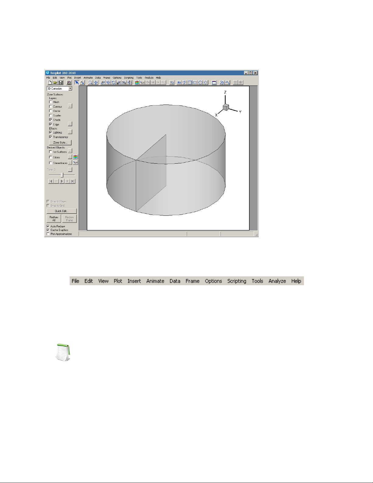
1 - 1 Interface

Five major sections make up the Tecplot 360 interface

Menu bar

and Toolbar

Workspace

Sidebar Status

1 - 1.1 Menubar

The menu bar offers rapid access to most of Tecplot 360’s features.

Tecplot 360’s features are organized into the following menus:

• File - Use the File menu to read or write data files and plot layouts, print and export plots, and

set configuration preferences.

• Edit - Use the Edit menu to select, undo, cut, copy, paste, and clear objects, open the Quick
Edit dialog, and change the draw order for selected items (push or pop).

Cut, Copy, and Paste work only within Tecplot 360. To place a graphic image of your
layout into another program, use Copy Plot to Clipboard. This option is available on
Windows® and Macintosh® platforms.

• View - Use the View menu to manipulate the point of view of your data, including scale, view
range, and 3D rotation. You can also use the View menu to copy and paste views between
frames.

The View menu includes the following convenient sizing options:

• Fit Everything (3D Only) - This options resizes plots so that all data points, text, and

geometries are included in the frame.

• Fit Surfaces (3D Only) - This option resizes plots so that all surfaces are included in the

frame, excluding any volume zones.

14

Interface

• Fit to Full Size - This option fits the entire plot into the frame. This option does not

affect the axis ranges.

• Nice Fit to Full Size - This option sets the axis range to begin and end on major axis

increments (if axes are dependent, the vertical axis length is adjusted to accommodate a
major tick mark).

• Data Fit - This option fits the data points to the frame.

• Make Current View Nice - This option modifies the range on a specified axis to fit the

minimum and maximum of the variable assigned to that axis, and then snaps the major
tick marks to the ends of the axis. (If axis dependency is not set as independent, this may
affect the range on another axis.)

• Center - This option moves the plot image so that the data points are centered within

the frame. (Only the data is centered; text, geometries, and the 3D axes are not
considered.)

• Plot - Use the Plot menu to control the style of your plots. The menu items available are
dependent upon the active plot type (chosen in the Sidebar).

• Insert - Use the Insert menu to add text, geometries (polylines, squares, rectangles, circles, and
ellipses), or image files. If you have a 3D zone, you may also use the Insert menu to insert a
slice. If the plot type is set to 2D or 3D Cartesian, you may insert a streamtrace.

• Animate - Use the Animate menu to animate IJK Planes, IJK Blanking, iso-surfaces, mappings,
slices, streamtraces, time, and zones.

• Data - Use the Data menu to create, manipulate, and examine data. Types of data
manipulation available in Tecplot 360 include zone creation, interpolation, triangulation, and
creation or alteration of variables.

• Frame - Use the Frame menu to create, edit, and control frames.

• Options - Use the Options menu to control the attributes of your workspace, including the
color map, paper grid, display options, and rulers.

• Scripting - Use the Scripting menu to play or record macros, and to access the Quick Macros
Panel dialog.

• Tools - Use the Tools menu to launch the Quick Edit dialog or an add-on.

• Analyze - Use the Analyze menu to examine grid quality, perform integrations, generate
particle paths, extract flow features, and estimate numerical errors.

• Help - Choose “Tecplot 360 Help” from the Help menu to get specific, complete help on
features or operations within Tecplot 360. By choosing “About Tecplot 360” from this menu,
you can obtain specific information about your license.

1 - 1.2 Sidebar

The Sidebar provides easy access for frequently used plot controls. The functions available in the Sidebar
depend on the plot type of the active frame. For 2D or 3D Cartesian plot types, you can add or subtract
zone layers, zone effects, and derived objects from your plot using the Sidebar. For line plots (XY and
polar) you can add or subtract mapping layers using the Sidebar.

To customize your plot, simply:

• Select a plot type from the Plot Types

• Use the toggle switches to add or subtract Zone Surfaces
the Zone Style/Mapping Style dialogs to further customize your plot by adding or subtracting

drop-down menu in the Sidebar.

, Zone Effects, or Derived Objects. Use

15

zones from specific plot layers/mappings, changing the way a zone or group of zones is
displayed, or changing various plot settings.

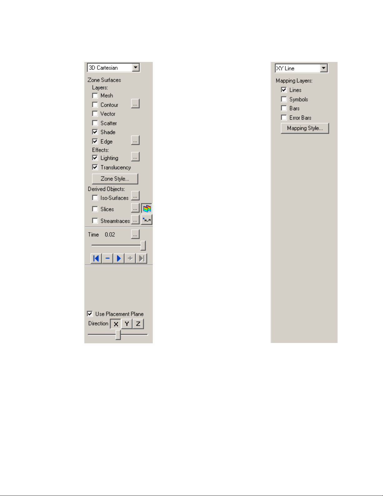
Figure 1-1. The Tecplot 360 Sidebar
for a field plot (left) and a line plot
(right).

The features available in the
Sidebar are dependent upon the
plot type.

For 3D Cartesian plots, you may
add and subtract zone layers,
derived objects, and effects for
your plot. You may also use the
Placement Plane for positioning
some 3D objects (3D plots only).

For 2D Cartesian plots (not
shown), you may add and subtract
zone layers and some derived
objects for your plot. For field plots
(3D or 2D), you may animate
transient data directly from the
Sidebar. For Line plots you may
add and subtract map layers. XY
Line plots have more available
map layers than polar line plots.

Plot Types

The Plot Type, combined with a frame’s dataset, active layers, and their associated attributes, define a plot.
Each plot type represents one view of the data. There are five plot types available:

• 3D Cartesian - 3D plots of surfaces and volumes.

• 2D Cartesian - 2D plots of surfaces, where the vertical and horizontal axis are both dependent
variables (i.e. x = f(A) and y = f(A), where A is another variable).

• XY Line - Line plots of independent and dependent variables on a Cartesian grid. Typically the
horizontal axis (x) is the independent variable and the y-axis a dependent variable, y = f(x).

• Polar Line - Line plots of independent and dependent variables on a polar grid.

• Sketch - Create plots without data such as drawings, flow charts, and viewgraphs.

16

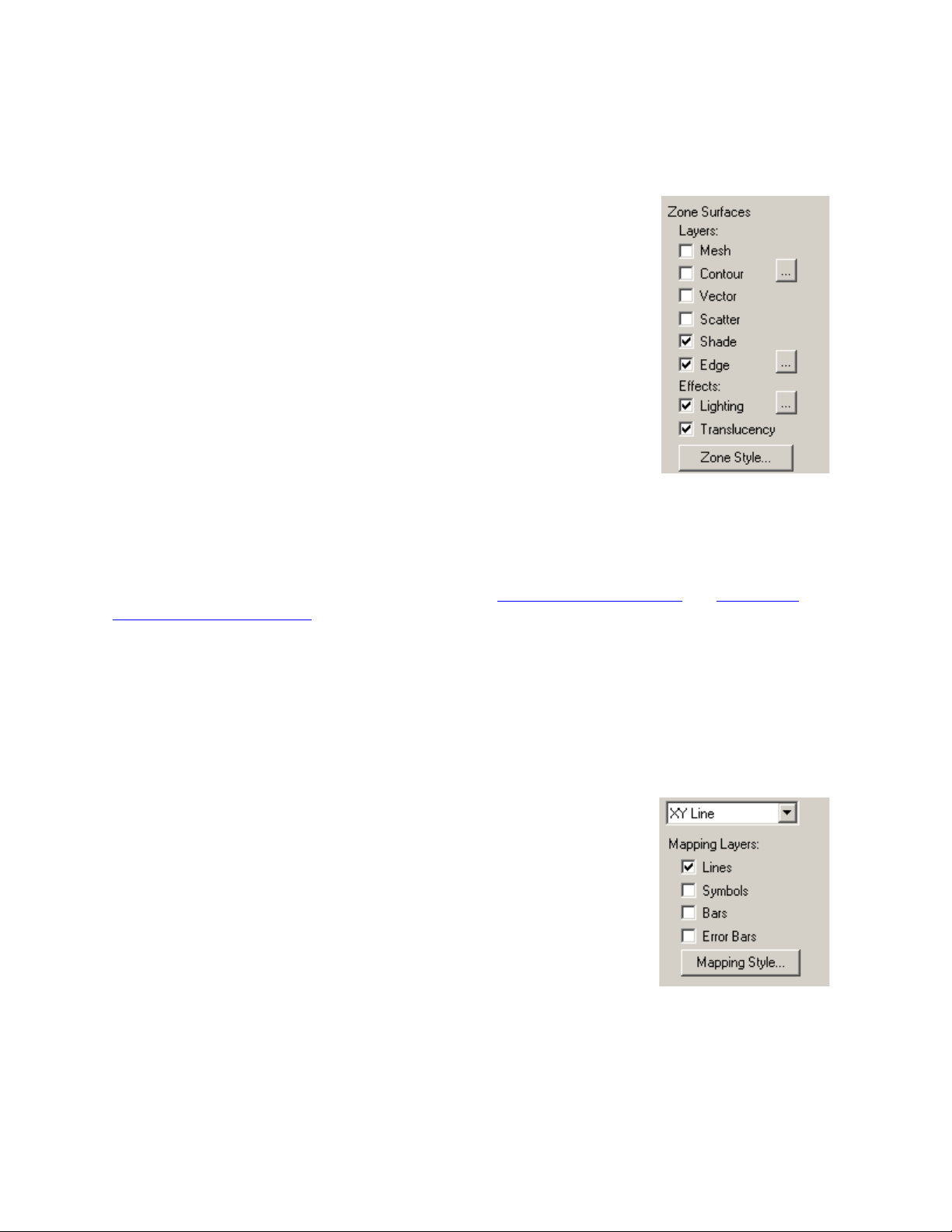
Zone Surfaces

Zone Lay ers

A layer is a way of representing a frame’s dataset. The complete plot is the
sum of all the active layers, axes, text, geometries, and other elements added
to the data plotted in the layers. The six zone layers for 2D and 3D Cartesian
plot types are:

• Mesh - A grid of lines connecting the data points within each zone.

• Contour - Iso-valued lines, the region between these lines can be set

to contour flooding.

• Vector - The direction and magnitude of vector quantities.

• Scatter - Symbols at the location of each data point.

• Shade - Used to tint each zone with a solid color, or to add light-

source shading to a 3D surface plot. Used in conjunction with the
Lighting zone effect you may set Paneled or Gouraud shading.
Used in conjunction with the Translucency zone effect, you may
create a translucent surface for your plot.

• Edge - Zone edges and creases for ordered data and creases for

finite element data.

Interface

Zone Effects

For 3D Cartesian plot types, use the Sidebar to turn lighting and translucency on or off. Only shaded and
flooded contour surface plot types are affected. Refer to Chapter 12: “Shade Layer”

“Translucency and Lighting” for additional information.

and Chapter 13:

Zone Style

Select the [Zone Style] button to launch the Zone Style dialog. The Zone Style dialog is used to customize
the zone layers that you have added to your plot. Refer to the chapter for each zone layer for details on
working with the Zone Style dialog.

Map Layers

A layer is a way of representing a frame’s dataset. The complete plot is the
sum of all the active layers, axes, text, geometries, and other elements added
to the data plotted in the layers.

The four XY Line map layers are:

• Lines - Plots a pair of variables, X and Y, as a set of line segments or

a fitted curve.

• Symbols - A pair of variables, X and Y, as individual data points

represented by a symbol you specify.

• Bars - A pair of variables, X and Y, as a horizontal or vertical bar

chart.

• Error Bars - Allows you to add error bars to your plot.

17

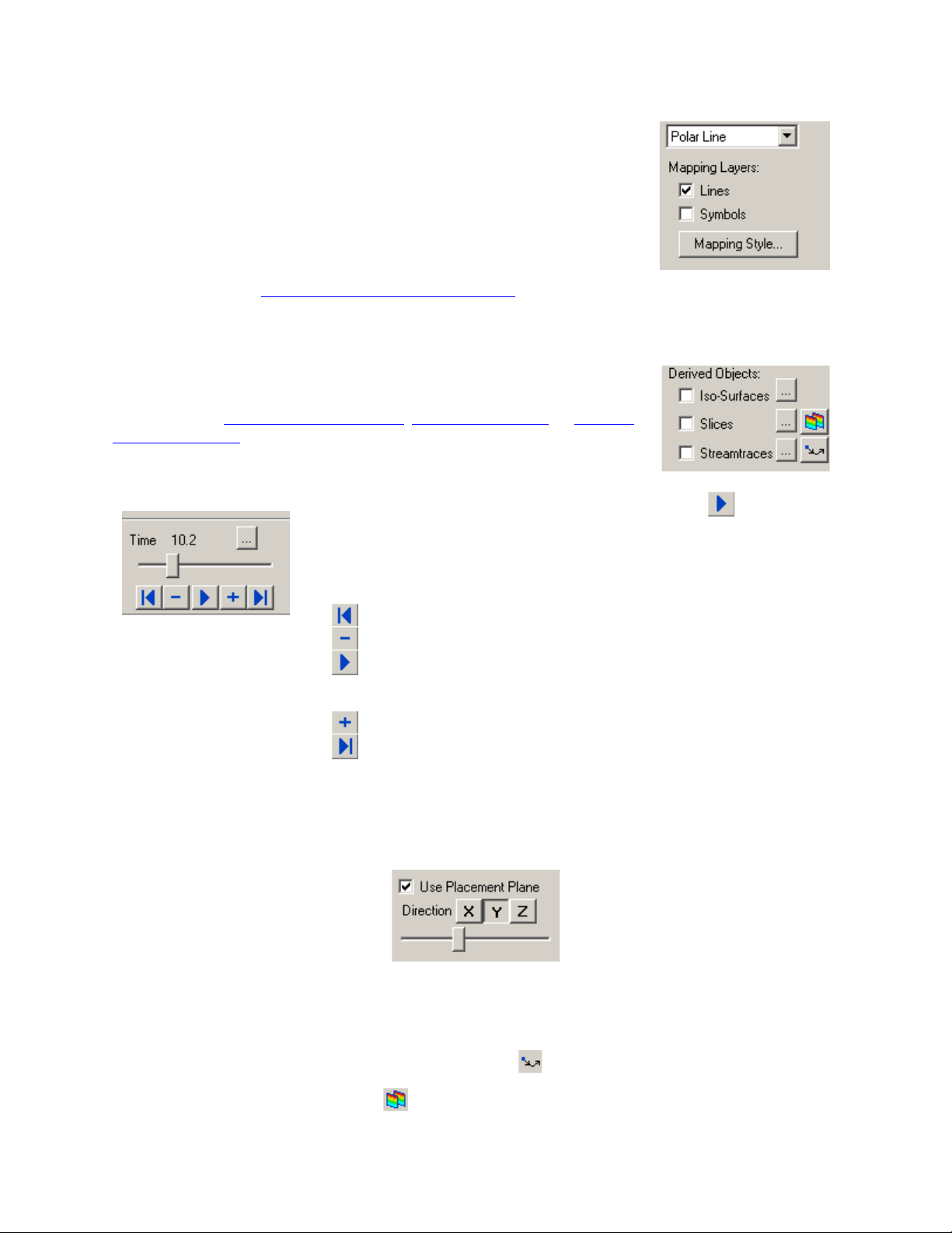
The two map layers for Polar Line are:

• Lines - A pair of variables, X and Y, as a set of line segments or a

fitted curve.

• Symbols - A pair of variables, e.g. X and Y, as individual data

points represented by a symbol you specify.

Select the [Mapping Style] button to launch the Mapping Style dialog. The
Mapping Style dialog allows you to customize the style settings for each of
the plot layers and specify the points to plot. The pages of the dialog are
discussed in detail in Chapter 6: “XY and Polar Line Plots”

.

Derived Objects

For Cartesian plot types (2D and 3D): Toggle-on Iso-surfaces, Slices, or
Streamtraces from the Sidebar to add any or all of these elements to your plot.
Their corresponding Details dialogs can be accessed via the Details [...]
button. Refer to Chapter 16: “Iso-surfaces”

15: “Streamtraces” for details on working with these objects.

, Chapter 14: “Slices”, or Chapter

Transient Controls

When working with transient data, simply press the Play button in the
Sidebar to animate over time. The active frame will be animated from the
Current Solution Time to the last time step. You may also drag the slider to
change the Current Solution Time of your plot.

The Animation Controls have the following functions:

• – Jumps to the Starting Value.

• – Jumps toward the Starting Value by one step.

• – Runs the animation as specified by the ‘Operation’ field of the
Time Details dialog. The Play button becomes a Stop button while the
animation is playing.

• – Jumps toward the Ending Value by one step.

• – Jumps to the Ending Value.

Use the Details [...] button to launch the Time Details dialog.

Placement Plane

When you are using certain tools to add objects to your plot, toggle-on “Use Placement Plane” in the

Sidebar to place them along a given plane (3D Plots only). Use the [X],[Y], and [Z] buttons to select the
plane to use, and use the slider to reposition the Placement Plane. The Placement Plane will appear as a
gray slice in your plot. The Placement Plane is available for:

Placing streamtraces (using the Add Streamtrace Tool )

Placing slices (using the Slice Tool )

18

Interface

Adding Contour Levels (using the Add Contour Level Tool )

Deleting Contour Levels (using the Remove Contour Level Tool )

Probing (using the Probing tool )

Snap Modes

Snap Modes allow you to place objects precisely by locking them to the nearest reference point, either on
the axis grid or on the workspace paper.

• Snap to Grid - Constrain object movement to whole steps on the axis grid. This can be useful
for aligning text and geometries with specific plot features.

• Snap to Paper - Constrain object movement to whole steps on the paper's ruler grid. This can
be useful for positioning frames precisely for printing, or for absolute positioning of text,
geometries, and other plot elements.

Details Button

The [Details] button is located immediately below the snap modes. It is context sensitive. Use this button
to call up the dialog most directly applicable to your current action. When the currently selected tool is
either the Selector or the Adjustor , but no objects are selected in the workspace, the [Details]
button is labeled [Quick Edit]. Otherwise, the button is labeled Object Details
and Tool Details

when your mouse cursor is not in “selector” mode and an object is not selected.

when an object is selected

Object Details

The [Object Details] button in the Sidebar calls up the dialog that most closely reflects the current state of
the cursor. For example, if you select a legend and then [Object Details], the Legend dialog will open.

Tool Details

[Tool Details] calls up the dialog related to the current state of the cursor. For example, if a rotate tool is
selected, [Tool Details] calls up the 3D Rotate dialog.

Redraw Buttons

The redraw buttons allow you to keep your plot up to date: [Redraw All] CTRL-D redraws all frames
(SHIFT-[Redraw All] completely regenerates the workspace); [Redraw] CTRL-R redraws only the active
frame.

Auto Redraw

Use Auto Redraw - When selected, the plot will be automatically redrawn, whenever style or data
changes. Some users prefer to turn this option off while setting multiple style settings and then manually
press the [Redraw] or [Redraw All] button on the Sidebar to see a full plot.

You can interrupt an auto-redraw at any time with a mouse click or key press.

19

Cache Graphics

Tecplot 360 uses OpenGL® to render plots. OpenGL provides for the ability to cache graphic instructions
for rendering and can re-render the cached graphics much faster than if Tecplot 360 sends the instructions
again. This is particularly true for interactive manipulation of a plot. However, this performance potential
comes at the cost of using more memory. If the memory need is too high, the overall performance could be
less. There are three graphics cache modes: cache all graphics, cache only lightweight graphics objects, and
do not cache graphics.

When “Cache Graphics” is selected in the Sidebar, Tecplot 360 assumes there is enough memory to
generate the graphics cache. Assuming this is true, Tecplot 360’s rendering performance will be optimal
for interactive manipulation of plots.

When memory constraints are very limited, consider toggling-off “Cache Graphics”. If you intend to
interact with the plot, also consider setting the Plot Approximation mode set to “All Frames Always
Approximated”.

See Section “Graphics Cache”

on page 487 for more information.

Plot Approximations

When Plot Approximation is selected and if the number of data points is above the point threshold, an
approximate plot for style, data, and interactive view changes is rendered. The approximate plot is
followed immediately by the full plot. This option provides for good interactive performance with the
final plot always displayed in the full representation.

See Section “Plot Approximation”

on page 486 for more information.

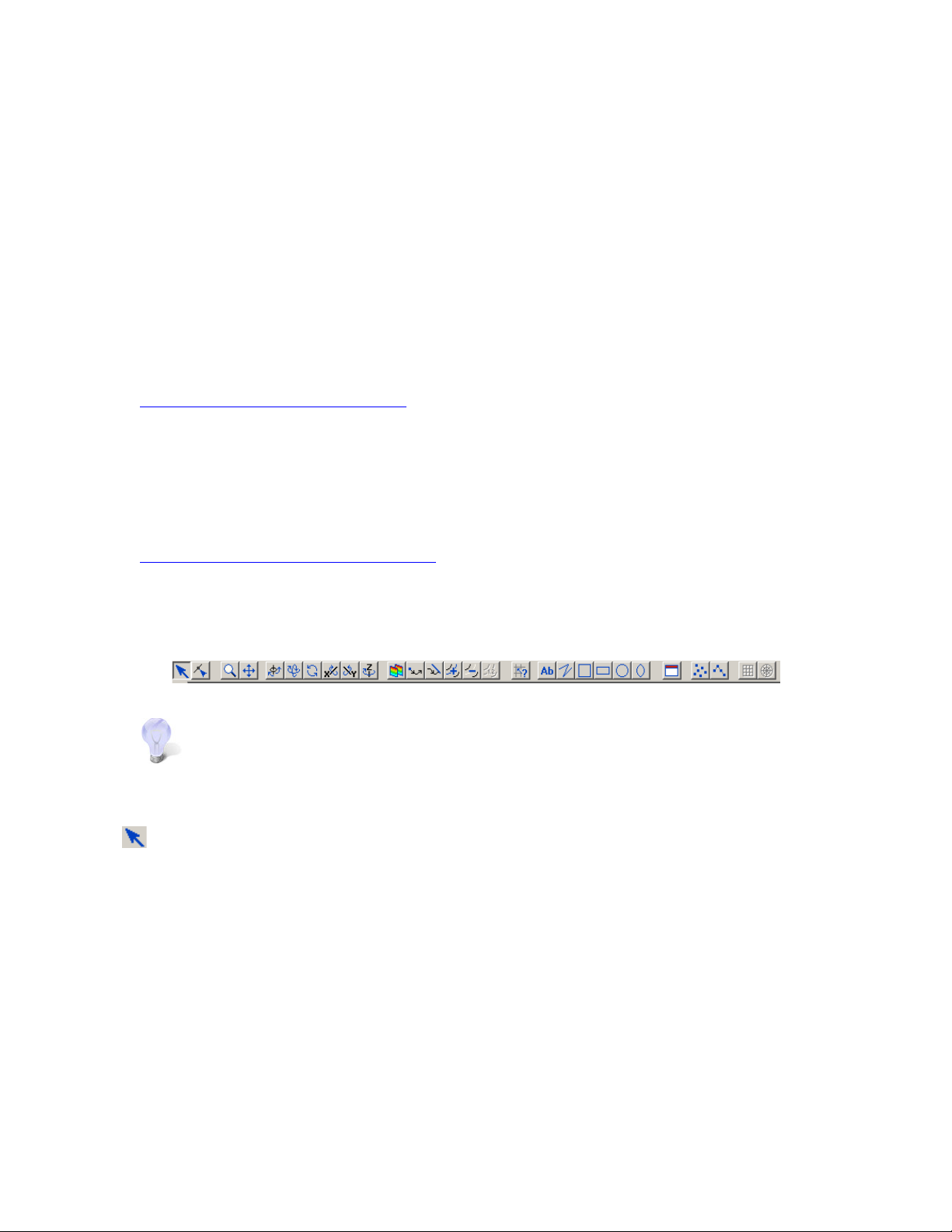
1 - 1.3 Toolbar

Each of the tools represented in the Toolbar changes the mouse mode and allows you to interactively edit
your plot.

Double-click on a tool to launch the Details dialog associated with the tool.

Selector Tool

Use the Selector tool to select objects in your workspace. The selected objects can be modified using

the Quick Edit dialog and (in some cases) the Selector tool itself.

The following objects can be moved (translated) using the Selector tool:

• frames

• axis grid area

• text

• geometries

• contour labels

• streamtraces

• streamtrace termination line

• legends

• 3D frame axis

20

Interface

To select an object and open that object's attributes dialog, either double-click on any object or drag the
cursor to select groups of objects (calls up Group Select dialog). Select the [OK] button, then select [Object
Details].

Adjustor Tool

Use the Adjustor tool to perform any of the following modifications to your plot and data:

• Location of individual or groups of data points in the grid.

• Values of the dataset variables at a particular point.

• Length or placement of individual axes (2D Cartesian and XY Line plot types only).

• Spacing between an axis label and its associated axis (2D Cartesian and XY Line plot types

only).

• Shape of a polyline.

For all other scenarios, the behavior of the Adjustor mode is identical to that of the Selector tool.

The Adjustor tool can alter your data. Be sure you want to use the Adjustor tool before
dragging points in the data region.

To select multiple points - You can either SHIFT-click after selecting your initial point to select additional
points, or you can draw a group select band to select the points within the band. (In line plots, you can
select points from only one mapping at a time.)

Once you have selected all desired points, move the Adjustor over the selection handles of one of the
points, then click-and-drag to the desired location of the first data point. The other selected points will
move as a unit with respect to the chosen data point, maintaining their relative positions.

For XY Line plots, if several mappings are using the same data for one of the variables,
adjusting one of the mappings will result in simultaneous adjustments to the others. You
can avoid this by pressing the
point. The

H and V keys restrict the adjustment to the horizontal and vertical directions,

H or V key on your keyboard while adjusting the selected

respectively.

Group Select

The Group Select dialog is opened when you select a group of objects with the Selector or Adjustor tool.

The Group Select dialog allows you to specify the following object types (if the selection rectangle does
not include a specific object, its associated check box is inactive):

• Text

• Geometries

• Frames

• Zones or Mappings

• Axis Grid Area

• Contour Labels

• Streamtraces

The Group Select dialog offers the following attribute filters:

• Geoms of Type - Choose geometries of a particular type from the drop-down menu.

21

• Geoms with Line Pattern - Choose all geometries having a particular line pattern.

• Text with Font - Choose all text displayed in a particular font.

• Objects with Color - Choose all objects of a particular color. You choose the appropriate color

from the Select Color dialog.

Zoom Tool

Zoom into or away from the plot.

When a mouse-click occurs (without dragging), the zooming is centered at the location of your click.

There are two zoom modes: plot zooming and paper zooming.

For plot zooming - drag the magnifying glass cursor to draw a box around the region that you want to fit
into the frame. The box may be larger than the frame. Making the box larger than the frame zooms away
from the plot. The region within the view box will be resized to fit into the frame.

If Snap to Grid (located in the Sidebar) is selected, you cannot make the zoom box
larger than the grid area.

To return to the previous view, choose “Last” from the View menu (CTRL-L). To restore the original 2D
view, choose” Fit to Full Size (CTRL-F)”.

The results of plot zooming for the 2D plot type are dependent upon the axis mode selected in the Axis
Details dialog (accessed via the Plot menu):

• 2D Independent Axis Mode - Allows the selected region to expand to exactly fit in the frame.
The axes are rescaled independently to fit the zoom box.

• 2D Dependent Axis Mode - In dependent mode, the axes are not fit perfectly to the zoom box.
The longest dimension from the zoom box is applied to an associated axis, and the other axis is
resized according to the dependency relation.

For paper zooming - SHIFT-drag the magnifying glass cursor to draw a box about the region that you
want to magnify. The plot is resized so that the longest dimension of the zoom box fits into the workspace.
You can fit one or all frames to the workspace by using the “Fit Selected Frames to Workspace” or “Fit All
Frames to Workspace” options from the View>Workspace menu. To return to the default paper view,
choose “Fit Paper to Workspace” from the View>Workspace menu.

Clicking anywhere in your plot while the zoom tool is active will center the zoom around
your click. Alternatively, CTRL-click centers the plot on the point that was clicked and
zooms out.

Use the center mouse button and drag (or hold down the rollerball and drag) to
interactively zoom into or out of the plot.

Translate Tool

Use the Translate/Magnify tool to translate or magnify data within a frame or the paper within the

workspace.

22

Interface

While in Translate/Magnify mode, drag the cursor to move the data with respect to the frame, or SHIFT­drag to move the paper with respect to the workspace.

Use the right mouse button to interactively translate objects. You can rescale your image
by pressing “+” to magnify, “-” to shrink. If you are SHIFT-dragging to move the paper,
the rescale buttons “+” and “-” will magnify or shrink the paper, as long as you have the
mouse button depressed.

Three-dimensional Rotation

There are six 3D rotation mouse modes:

Spherical - Drag the mouse horizontally to rotate about the Z-axis; drag the mouse vertically to

control the tilt of the Z-axis.

Rollerball - Drag the mouse in a direction to move with respect to the current orientation on the

screen. In this mode, your mouse acts much like a rollerball.

Twis t - Drag the mouse clockwise around the image to rotate the image clockwise. Drag the

mouse counterclockwise around the image to rotate the image counterclockwise.

X-axis - Drag the mouse to rotate the image about the X-axis.

Y-axis - Drag the mouse to rotate the image about the Y-axis.

Z-axis - Drag the mouse to rotate the image about the Z-axis.

Once you have selected a rotation mouse mode, you can quickly switch to any of the others using the
following keyboard shortcuts:

Drag Rotate about the defined rotation origin with your current Rotate tool.

ALT-drag Rotate about the viewer position using your current Rotate tool.

Middle-click-and-drag/ALT­right click-and-drag

Right-click-and-drag Translate the data.

Smooth zoom in and out of the data.

This option can be used without first selecting a rotation mouse mode. Simply

CTRL-right-click-and-drag

C Move rotation origin to probed point, ignoring zones.

hover over your intended point of origin, and then CTRL-right-click-and-drag
to translate the image.

23

Move rotation origin to probed point of data.

O

R Switch to Rollerball rotation.

S Switch to Spherical rotation.

T Switch to Twist rotation.

X Switch to X-axis rotation.

Y Switch to Y-axis rotation.

Z Switch to Z-axis rotation.

This shortcut can be used without first selecting a rotation mouse mode.
Simply hover over your intended point of origin, type O, and then
right-click-and-drag to rotate the image.

Slice Tool

Use the Slicing tool to add a slice interactively by clicking anywhere in your plot. You can also use

this tool to control your slice(s) interactively.

The following keyboard/mouse options are available when the Slice tool is active:

Primary Slices, Start End Slices Active - Turn on intermediate slices (if not

+

already active) and adds a slice.
Primary Slices active [ONLY] - Turns on Start/End Slices and adds a slice.
Start/End Slices active [ONLY] - Turns on Start/End Slices and adds a slice.

CTRL-

Primary Slices, Start End Slices Active - Removes start and end slices.

-

Click/Drag

ALT-click/ALT-drag

SHIFT-click

SHIFT-drag

I, J, K (ordered zones only) Switch to slicing constant I, J, or K-planes respectively.

X, Y, Z Switch to slicing constant X, Y, or Z-planes respectively.

1-8 Numbers one through eight switch to the corresponding slice group.

Primary Slices active [ONLY] - Removes the primary slice.
Start/End Slices active [ONLY] - Removes the Start and End Slices.

Updates the position of the primary slice (if active). If only start and end slices
are visible, click updates the position of the starting slice.

Determine the XYZ-location by ignoring zones and looking only at derived
volume objects (streamtraces, slices, iso-surfaces).

Switches from one Primary slice to Start/End Slices by adding a slice.

Move the start or end slice (whichever is closest to the initial click location).
Show Start/End Slices is activated, if necessary.

24

Add Streamtrace

Select the Add Streamtrace tool to add a streamtrace interactively by clicking anywhere in your plot.

Select the number of streamtraces to include with each click (rake) using 1-9 on the keyboard.

Keyboard Shortcuts

DSwitch to streamrods
RSwitch to streamribbons
SSwitch to surface lines
VSwitch to volume lines
1-9Change the number of streamtraces to be added when placing a rake of

streamtraces
SHIFT - Draws a rake on concave 3D volume surfaces. These rakes are normally not

drawn, as they occur outside of the data
Refer to Chapter 15: “Streamtraces”

for more information.

Streamtrace Termination Line

Select the Add Streamtrace Termination Line tool to add a streamtrace termination line

interactively.

Interface

To draw a Streamtrace Termination Line:

• Move the cursor into the data region.

• Click once at the desired starting point for the line.

• Click again at each desired break point.

• When the polyline is complete, double-click on the last point of the polyline, or press ESC on

your keyboard.

• The drawn polyline ends any streamtraces that pass through it.

Add Contour Level

Select the Add Contour Level tool to add a contour level by clicking anywhere in the active data

region. A new contour level, passing through the specified location, is calculated and drawn.

The following keyboard and mouse shortcuts are related to the Add Contour Level tool.

ALT-click Place a contour line by probing on a streamtrace, slice, or iso-surface.

Click Place a contour line.

CTRL-Click

Drag Move the new contour line.

-

Replace the nearest contour line with a new line.

Switch to the

Delete Contour Level tool.

25

Delete Contour Level

Select the Delete Contour Level tool to delete a contour level by clicking anywhere in the active
data region. The contour line nearest the specified location is deleted.

Use the “+” key to switch to the Add Contour Level tool and the “-” key to switch back to
the Delete Contour Level tool.

Add Contour Labels

Select the Add Contour Label tool to switch to the Contour Label mode, enabling you to add a

contour label by clicking anywhere in the active data region.

A contour label is added to the plot at the specified location; its level or value information is taken from
the nearest contour line. This allows you to place labels at a slight offset from the lines they label.

The Contour type must be lines or lines and flood in order for this tool to be active. You
can set the contour type on the Contour page of the Zone Style dialog.

Probe Tool

Select the Probe At Tool to probe for values of the dataset's variables at a particular point.

To obtain interpolated values of the dataset variables at the specified location, click at any point in the data
region.

To obtain exact values for the data point nearest the specified location, CTRL-click at the desired location.

For XY plots, when you move into the axis grid area, the cursor cross hair is augmented
by a vertical or horizontal line, depending on whether you are probing along the X-axis
or the Y -axis. You can change the axis to probe simply by pressing X to probe the X-axis
or Y to probe the Y-axis.

Insert Text

Select the Add Text tool to add text to any frame.

Insert Geometries

Use the corresponding geometry buttons in the Toolbar to insert geometries into your plot.

Polylines

Squares

Rectangles

26

Circle

Ellipse

Create New Frame

Select the Create Frame tool to create a new frame.

To add a frame:

• Click once in the workspace to anchor one corner of the frame.

• Drag the diagonal corner until the frame is the desired size and shape.

If you have data loaded before you create a new frame, you can attach the existing
dataset to the new frame by changing the plot type.

Extract Discrete Points

Select the Extract Discrete Points tool to extract selected points to a data file or a new zone.

To select points:

• Click your left-hand mouse button at each location where you would like to extract a point.

• To end extraction, either double-click on the last point, or right click, or press the ESC key.

• The Extract Data Points dialog appears; use it to specify how many points to extract and how

to save the data.

Interface

Extract Points along Polyline

Select the Extract Line tool to extract points along a specified polyline to a data file or a new zone.

To select points:

• Click your left-hand mouse button at each location where you would like to extract a point.

• To end extraction, either double-click on the last point, or right click, or press the ESC

• The Extract Data Points dialog appears; use it to specify how many points to extract and how

to save the data.

key.

Create Rectangular Zone

Select the Create Rectangular Zone tool to add 2D rectangular zones to the active dataset.

To create a rectangular zone:

• Click once in the active data region to anchor one corner of the zone.

• Drag the diagonal corner until the zone is the desired size and shape. The new zone created is

IJ-ordered.

To specify the maximum I-index and J-index, use the Create Rectangular Zone dialog (accessed via
Data>Create Zone).

The active frame must have a dataset attached to it in order for this tool to be active.
This tool is available in 2D plots only.

Create Circular Zone

Select the Create Circular Zone tool to add new 2D circular zones to the active dataset.

27

To create a circular zone:

• Click once in the active data region to specify the center of the zone.

• Drag until the zone has the desired radius. The new zone created is IJ-ordered.

To specify the maximum I-index and J-index, use the Create Circular Zone dialog (accessed via
Data>Create Zone).

The active frame must have a dataset attached to it in or der for the Create Circular Z one
tool to be active. This tool is available in 2D plots only.

1 - 1.4 Status Line

The status line appears along the bottom of the Tecplot 360 window to give “hover help”, as well as a
progress bar and information when Tecplot 360 computes calculations. The hover help appears when you
move the pointer over a tool in the Toolbar, a button or item in the sidebar, or a menu item, and gives a
description of the control.

A progress bar and information about the calculation Tecplot 360 is completing appears in the status line
during lengthy calculations or other longer operations.

1 - 1.5 Tecplot 360 Workspace

In the Tecplot 360 workspace, you can create sketches and plots. You can create each sketch or plot within
a window called a frame. Each visible measure of the workspace is called a page. The current state of the
workspace, including the sizing and positioning of frames, the number and contents of pages, the location
of the data files used by each frame, and all current attributes for all frames, makes up a layout. By default,
the workspace displays a representation of where the paper plots are drawn, as well as a reference grid
and rulers. The frame most recently selected is called the active frame.

You can include multiple pages in your layout. To create a new page, modify pages or move between
them, use the Quick Macro Panel. See Section 28 - 2.1 “Quick Macro Panel”
the panel.

for more information about

28

Interface

1 - 1.6 Quick Edit

The map and zone layer controls affecting how the individual layers are drawn can be altered using
controls on the Sidebar. You can also control many of these attributes using the Quick Edit dialog.

The Quick Edit dialog is accessed via the [Quick Edit] button located at the bottom of the Sidebar when
the mouse-mode is a standard arrow (i.e. you are using either the Selector Tool
are in a different mouse mode, or you have selected a Text or Geometry object, the Object Details

Details will be launched in lieu of the Quick Edit dialog.

To use the Quick Edit dialog, select one or more objects in the workspace, then select the appropriate
button in the dialog to change the attributes of the selected object(s). The functionality of each button is
described in the following sections.

or Adjustor Tool). If you

or Tool

Mesh

This area of the Quick Edit dialog controls whether the mesh is displayed for selected zones, and if so,
using which types of mesh. The following options are available:

• Y - Show the mesh for the selected zones. The first time you turn on the Mesh layer by either

the Quick Edit dialog or the Zone Style dialog, a dialog appears asking if you wish it
activated. Select [Yes] to confirm turning on the layer.

• N - Turn off the mesh for the selected zones.

29

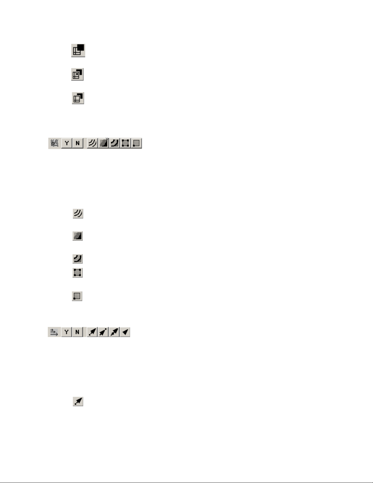
• Wire Frame - Mesh lines are drawn underlying all other field layers (i.e., Contour,

Vector, Scatter, Shade); hidden lines are not removed.

• Overlay - Mesh lines are drawn above all other field plot layers except vectors and scatter

symbols.

• Hidden - Similar to Overlay, except that in the 3D Cartesian, plot type hidden lines are

removed from behind the mesh. In essence, the cells of the mesh are opaque. Surfaces and
lines that are hidden behind another surface are removed from the plot.

Contour

This area of the Quick Edit dialog controls whether contours are displayed for selected zones, and if so,
using which plot type. The following options are available:

• Y - Show the contours for the selected zones. The first time you turn on the Contour layer by

either the Quick Edit dialog or the Zone Style dialog, a dialog appears asking if you wish it
activated. Select [Yes] to confirm turning on the layer.

• N - Turn off the contour for the selected zones.

• Lines - Plots contour lines. If you choose this plot type, you can use the Cont Color

attribute to specify Multi-Color to make the line color vary with the contour-variable value.

• Flood - Flood the area between adjacent contour lines with a color according to the value

of the contour variable, number of contour levels, and the Color Map.

• Both Lines and Flood - Contour lines are drawn with color flooding between them.

• Average Cell - Each cell or element is flooded with one solid color based upon the

average value of the contour variable at the data points of the cell or element.

• Primary Value - Each cell or element is flooded with one solid color based upon the

primary cell value.

Vector

This area of the Quick Edit dialog controls whether vectors are displayed for selected zones, and if so,
using which plot type. The following options are available:

• Y - Show the vectors for the selected zones. The first time you turn on the Vector layer by either

the Quick Edit dialog or the Zone Style dialog, a dialog appears asking if you wish it
activated. Select [Yes] to confirm turning on the layer.

• N - Turn off the vectors for the selected zones.

• Tail at Point - Display regular vectors – a simple stick vector with length proportional to

the local magnitude. The tail of the vector is positioned at the data point.

30

Interface

• Head at Point - Display regular vectors – a simple stick vector with length proportional to

the local velocity magnitude (the square root of the sum of the squares of the vector
components). The head of the vector is positioned at the data point.

• Anchor at Midpoint - Display regular vectors – a simple stick vector with length

proportional to the local velocity magnitude. The midpoint of the vector is positioned at the
data point.

• Head Only - Display vectors as heads only, without the vector shaft.

Scatter

This area of the Quick Edit dialog controls whether scatter symbols are displayed for selected zones, and
if so, whether to use plain or filled symbols. The following options are available:

• Y - Show the scatter symbols for the selected zones. The first time you turn on the Scatter layer

by either the Quick Edit dialog or the Zone Style dialog, a dialog appears asking if you wish it
activated. Select [Yes] to confirm turning on the layer.

• N - Turn off the scatter symbols for the selected zones.

• Plain - Use un-filled symbols for the scatter plot.

• Filled - Use filled symbols for the scatter plot.

Shade

This area of the Quick Edit dialog controls whether shading is used for selected zones. This option allows
you to turn off just the Shade layer for specific zones, without completely deactivating the zones. The
following options are available:

• Y - Show light-source shading for the selected zones. The first time you turn on the Shade layer

by either the Quick Edit dialog or the Zone Style dialog, a dialog appears asking if you wish it
activated. Select [Yes] to confirm turning on the layer.

• N - Turn off light-source shading for the selected zones.

Edge Border

This area of the Quick Edit dialog controls whether the zone edge border is displayed for selected ordered
zones, and if so, what edge type. The following options are available:

• Y - Show edges borders for the selected zones. The first time you turn on the Edge layer by

either the Quick Edit dialog or the Zone Style dialog, a dialog appears asking if you wish it
activated. Select [Yes] to confirm turning on the layer.

• N - Turn off edges for the selected zones.

• Show Entire Border - Shows border lines on all boundaries of the selected zone(s).

31

• Show Border Line - Shows the edge border line closest to the selected point.

• Hide Border Line - Hides the edge border line that is closest to the selected point.

• Show Only Nearest Border Line - Shows only the edge border line that is closest to the

selected point and hides all others.

• The first time you turn on the Line layer by either the Quick Edit dialog or the Mapping Style

dialog, a dialog appears asking if you wish it activated. Select [Yes] to confirm turning on the
layer.

Symbols Mapping Layer

This area of the Quick Edit dialog controls whether symbols are plotted at each data point, and whether
those symbols are filled or plain. The following options are available:

• Y - Show the symbol plots for the selected maps. The first time you turn on the Symbols layer

by either the Quick Edit dialog or the Mapping Style dialog, a dialog appears asking if you
wish it activated. Select [Yes] to confirm turning on the layer.

• N - Turn off the symbol plots for the selected maps.

• Plain - Use un-filled symbols for the scatter plot.

• Filled - Use filled symbols for the scatter plot.

XY Error Bars Mapping Layer

This area of the Quick Edit dialog controls whether error bars are displayed for the selected mappings,
and in which direction the error bars are drawn. The options are:

• Y - Show the error bars for the selected maps. The first time you turn on the Error Bars layer by

either the Quick Edit dialog or the Mapping Style dialog, a dialog appears asking if you wish
it activated. Select [Yes] to confirm turning on the layer.

• N - Turn off the error bars for the selected maps.

• Top - Error bar extends upward for positive values (and downward for negative values)

of the error bar variable.

• Bottom - Error bar extends downward for positive values (and upward for negative

values) of the error bar variable.

• Left - Error bar extends to the left for positive values (and to the right for negative values)

of the error bar variable.

• Right - Error bar extends to the right for positive values (and to the left for negative

values) of the error bar variable.

32

• Horizontal - Error bar extends both left and right.

Interface

• Vertical - Error bar extends both up and down.

• Cross - Error bar extends up, down, left, and right.

Bars Mapping Layer

This area of the Quick Edit dialog controls whether bars are plotted to represent each data point, and
whether those bars are filled or plain.

• Y - Show the selected maps as bar charts. The first time you turn on the Bars layer by either the

Quick Edit dialog or the Zone Style dialog, a dialog appears asking if you wish it activated.
Select [Yes] to confirm turning on the layer.

• N - Turn off bar charting for the selected maps.

• Plain - Use un-filled bars for the bar chart.

• Filled - Use filled bars for the bar chart.

Color

This area of the Quick Edit dialog controls color options for filled objects, lines, and text.

• Object-type - Use the Fill, Line, and Text radio buttons to identify the object-type to modify.

• Color - Select the [Color] button to activate the Select Color dialog. Multi color is not available

for line plots.

• X button - The behavior of the [X] button depends on the object-type selected.

• Fill - [X] turns off the fill color.

• Line - [X] causes the line color to match the fill color. If no fill color is specified, the [X]

button has no effect.

• Te xt - [X] has no effect.

Symbols

Use this region of the Quick Edit dialog to change the symbol for the Scatter Zone layer or Symbols Map
layer.

Use the [Size] button to specify the size of the scatter symbols as a percentage of the frame width (in the 2D
Cartesian plot type) or of the median-axis length (in the 3D Cartesian plot type).

33

Line Pattern

This area of the Quick Edit dialog controls the line pattern, pattern length, and line
thickness for all selected objects.

• Line Pttrn - Choose the line pattern for the selected zones.

• Pttrn Lngth - Specify the pattern length for the selected line pattern, as a
percentage of the frame width.

• Line Thcknss - Specify the line thickness for the vectors as a percentage of the
frame width.

Arrows

This area of the Quick Edit dialog controls arrowhead placement on polylines.

Arrowheads

This area of the Quick Edit dialog controls the type, size, and angle of arrowhead for both
selected vectors and selected polylines and vectors. The following options are available:

• Head Style - Choose the vector head style for the selected zones. The following
options are available:

• Plain - Display arrowheads as lines drawn from the head of the vector.

• Filled - Display arrowheads as filled triangles at the end of each vector.

• Hollow - Display arrowheads as hollow triangles at the end of each vector.

• Size - Specify the size of the arrowhead as a percentage of frame height.

• Angle (deg) - Specify the angle between the vector and the arrowhead.

• Enter Value - For both the [Size] and [Angle] buttons, you can choose “Enter” and type in an
exact percentage in the Enter Value dialog.

Font

This area of the Quick Edit dialog controls the font family and size used for selected text. (See Section 18 -

1.2 “Font Folders and Fallback” on page 273 for more information on how fonts work with Tecplot 360.)

The following options are available:

• Font menu - Select the font family.

• B, I, R - Select the boldface, italic, bold/italic, or regular version of the font.

• Size (%) - Specify the height for the text in frame units (i.e. as a percentage of frame height).

• Size (pt) - Specify the height for the text in points.

34

Getting Help

Order and Alignment

Use the Order and Alignment buttons of the Quick Edit dialog to align text within textboxes or the
alignment between selected geometries/textboxes.

• Left, Center, or Right - Use the Left, Center, or Right alignment buttons to align

text.

• To p or Bottom - Use the Top or Bottom alignment buttons to align selected geometries

and text with respect to one another.

• Push - Use the Push button to push the selected geometries, frames, or text to the bottom of the

draw order. If you select frames including the active frame and use the [Push] button, Tecplot
360 will activate the new topmost frame. Otherwise, the [Push] button will not affect the active
frame.

• Pop - Use the Pop button to pop the selected geometries or text to the top of the draw order. If

you select inactive frames and use the [Pop] button, Tecplot 360 will activate the newest
topmost frame. Otherwise, the [Pop] button will not affect the active frame.

For more information about active frames, see Section 2 - 3.1 “The Active Frame

Receives All Actions”.

1 - 2 Getting Help

Tecplot 360 features a fully integrated Help system. Quick help on menu items and Sidebar controls is
available from the status line or tool tips.

Detailed help is accessible by:

• Pressing the

Quick Edit dialog, or a menu, the
menu. Otherwise,

• Selecting “Contents” from the Help menu.

• Selecting Help on any dialog.

The Help dialog supports text search, has hypertext links, and provides detailed information on all menus
and dialogs.

Your an swer m ay be in Technical Support Notes at www.tecplot.com/support

If you are covered by Tecplot’s Software Maintenance Service, help is also available from 6:30 A.M. to 5
P.M. Pacific Standard Time from Tecplot Technical Support at 425.653.9393.

You may also send an e-mail to [e-mail]

F1 key anywhere in the Tecplot 360 window. If the pointer is over the Sidebar,

F1 key provides context-sensitive help on that control or

F1 calls up the Contents page of Help via your Web browser.

.

with your questions.

35

36

2

Using the Workspace

This chapter discusses the structures and features of Tecplot 360 that act the same regardless of the data
type or plot layers you are using. These include:

• Data Hierarchy

• Interface Coordinate Systems

and where they occur

• Frames

• Workspace Management Options Menu

your paper, as well as the ruler and grid, in order to precisely size and position objects. For in­depth information on Display Performance, refer to Section 32 - 3 “Performance Dialog”

• View Modification - The commands to zoom, translate, and fit plots within frames

• Edit Menu

to paste plot elements

- Areas in the workspace in which you can create plots and control formatting

- How Tecplot 360 manages data

- Tecplot 360’s use of different coordinate systems, and when

- Factors that determine the color and orientation of

- The commands to cut or copy plot elements from a workspace, and the command

2 - 1 Data Hierarchy

Tecplot 360 structures data in two levels: datasets, which display in frames, and zones, which make up a
dataset. Each dataset is composed of one or more zones, and each zone contains one or more variables. All
zones within a dataset contain the same set of variables.

37

This chart, Figure 2-1, displays a visual representation of Tecplot 360’s method of data hierarchy.

Figure 2-1. Data Hierarchy in Tecplot 360. Frames 1 & 2 display Dataset 1, and Dataset 1 contains three

zones from one data file. Frame 3 contains Dataset 2, which is composed of five zones (two
from data file 2 and three from data file 3).

2 - 1.1 Data Displays in Frames

Tecplot 360 always displays data in a window called a “frame”. By default, Tecplot 360 opens one frame
when you launch Tecplot 360 or open a new layout, but you can display multiple plots concurrently in
Tecplot 360 by adding additional frames. You can add frames to the workspace using the Frame menu.
You can display one dataset in one frame, or you can share one dataset between multiple frames. Using the
same dataset in multiple frames allows you to generate different plots of the same data. To learn more
about working with frames, go to Section 2 - 3 “Frames”

.

2 - 1.2 A Dataset Includes All Data in a Frame

A dataset is defined as “all of the data in a frame”. To create a dataset, load one or more data files into an
empty frame in Tecplot 360, or create a zone in a frame.

2 - 1.3 Datasets Are Made of Zones

A zone represents a subset of a dataset. A dataset can be composed of a single zone or several zones.
Zones are either defined in the data file or created directly in Tecplot 360. The number of zones in a dataset
is the sum of the number of zones in each of the data files included in the dataset.

Typically, a data file is divided into zones based on its physical coordinates. For example, a dataset of an
airplane many consist of a zone for each wing, each wheel, the nose, etc. Alternatively, zones may be

38

Interface Coordinate Systems

defined based on the material. For example, a dataset of a fluid tank may have a zone for the tank itself
and additional zones for each fluid inside the tank.

All zones in a given dataset must have the same variables defined for each data point.

2 - 2 Interface Coordinate Systems

Tecplot 360 incorporates a number of coordinate systems, including the paper, frame, and the physical
coordinate systems for the plot (2D, 3D, XY, or Polar). The origins of each coordinate system and their
relationship to one another is shown in Figure 2-2

.

Figure 2-2. Tecplot 360 Coordinate System. The physical coordinate system(s) of the dataset (for

example, 3D Cartesian or 2D Cartesian) are encompassed in the Frame Coordinate System.

The physical coordinate system (2D or 3D) depends on the plot type of the active frame. Two-dimensional
physical coordinates are often referred to as grid coordinates. The Grid coordinate system is aligned with
the coordinate system used by the plot axes; the Frame coordinate system is fixed to the frame and does
not change when the plot is zoomed, translated, or rotated.

In 2D Cartesian plots, objects such as text labels and geometries are drawn in either the Frame or the Grid
coordinate system. In 3D Cartesian plots, these objects are drawn in either the Frame coordinate system, or
in what is known as the Eye coordinate system. The eye coordinate system is aligned with the Grid
coordinate system; so objects drawn in the Eye coordinate system move with the data as you zoom and
translate, but remain fixed when you rotate the plot.

39

Figure 2-3 shows a 3D volume plot with streamribbons and a streamtrace termination line. This figure

illustrates how the termination points vary as the plot is rotated. Notice that the termination line itself
remains in place on the screen as the plot is rotated.

Figure 2-3. Rotating Volume streamtraces with a termination line in the eye coordinate system.

2 - 3 Frames

All plots and sketches display within frames. By default, the Tecplot 360 workspace contains one frame.
You may add additional frames, resize and reposition frames, modify background color, and specify
border and header appearance. Tecplot 360 acts upon only one frame, the The Active Frame Receives All

Actions, at any given time (except when frames are linked). The active frame displays with a darker and

thicker border than the inactive frames so that if you display multiple frames, you can easily see which
frame is active.

Tecplot 360 uses the height of the frame for objects scaled by frame units, such as font
size. When you enter a frame unit value into a dialog or when you set frame size and
position on the paper, you may specify a different unit system (inches, points,
centimeters, or pixels). Tecplot 360 automatically converts the values into frame units.

2 - 3.1 The Active Frame Receives All Actions

The active frame, indicated by default with a darker and thicker border, is the frame in your workspace
which operations affect. To make a frame the active frame, select anywhere inside that frame with your
Selector tool (or any other tool except the Create New Frame tool). Reference the following sections for
additional actions you can perform on frames.

2 - 3.2 Frame Creation

To create a new frame, which you can use to display a new dataset or another view of an already-loaded
data set, select the New Frame button in the toolbar. Or select “Create New Frame” from the Frame
menu. Selecting either the New Frame tool or “Create New Frame” in the Frame menu will change your
selector tool into a small “+” symbol. Click with this tool in your workspace where you want one corner of
your new frame, and drag across the workspace to where you would like the opposite corner of your new
frame.

Tecplot 360 will automatically make the new frame the active frame.

40

Frames

For optimal printing of your plot(s), draw frames that sit completely within the paper displayed in the
workspace. To view the paper coordinate system (to easily arrange frames for printing), go to
Options>Paper Setup and toggle-on “Show Paper on Screen”.

See Section 33 - 3.6 “Create Multiple Frames”

Data Set Inheritance After creating a new frame, you can assign the frame to share
the dataset of another frame by changing the frame order and the plot type of the new
frame. When you switch a frame without data out of Sketch plot type, Tecplot 360
searches for another frame with which to share data. It performs this search in the order
that the frames are drawn on-screen (which you can adjust by choosing “Order Fr ames”
from the Frame menu and choosing Draw Order from the List By menu), starting from
the top and moving down. The empty frame will inherit data from the first frame in the
draw order that contains data.

for information on simultaneously creating multiple frames.

2 - 3.3 Edit Active Frame

The Edit Active Frame dialog (accessed from the Frame menu) allows you to adjust the dimensions and
style of your active frame. When you are working with multiple frames, select a frame with your selector
tool to make that frame active. Then select “Edit Active Frame” from the Frame menu to adjust the
position and properties of that frame.

Frame Dimensions

You can size and position a frame by several methods. To use only your mouse, select the frame to activate
the resizing toggles (black boxes on the edges and corners of the frame). Click and drag on a resizing
toggle to resize a frame, or click and drag on an edge in a location without a resizing toggle to change the
frame location. To specify size or position with a dialog, select “Edit Active Frame” from the Frame menu.
To have Tecplot 360 resize frames for you, choose “Fit all Frames to Paper” from the Frame menu.

41

In the Edit Active Frame dialog, you may specify the exact
location for the frame’s left and top sides, along with width
and height.

• Left Side - Left edge of the frame, relative to the
workspace

• Top Side - Top edge of the frame, relative to the
workspace

• Width - Width of the frame (coordinates are: left
side to left side + width).

• Height - Height of the frame (coordinates are: top side to top side - height).

The units in the Frame Dimensions region of the dialog are based on the units set for the Ruler Spacing in
Options>Ruler/Grid.

You may also use the mouse or the arrow keys to resize and position frames. Click
anywhere on a frame’s header or border to activate resizing handles for the frame. To
scale frames proportionally (maintaining the vertical to horizontal aspect ratio) select the
frames, then press “+” on your keyboard to enlarge or “-” to reduce.

After selecting frames, you may position them using the arrow keys on your keyboard. You can move
frames up, down, left, or right in one-pixel increments for precise location.

To fit the active frame to the entire printable region of the paper (landscape
orientation), set Left Side=0.127, Top Side=0.125, Width=10.75, and Height=8.25. Or,
set Width=8.25 and Height=10.75 for portrait orientation. The pink border viewed
when “Show Paper on Screen” is toggled on in Options>Paper Setup marks the
printable region of the paper.

Frame Border and Header Controls

Use the Edit Active Frame dialog (accessed from the Frame menu) to adjust the frame border or header.

Toggling-off “Show Border” makes the frame border
invisible. To show a dashed line for invisible borders, go to
Options>Show Invisible Frame Borders. Use the
Thickness box in the Edit Active Frame dialog to adjust the
line thickness of the border.

Remember that Tecplot 360 uses a thicker border to
indicate the The Active Frame Receives All Actions

you change border settings, it may become difficult to determine which frame you have active.

The frame header displays when both “Show Border” and “Show Header” are toggled-on. If you turn off
the border by toggling-off “Show Border”, the header turns off as well.

The frame header contains user-configurable information which defaults to:

"&(FrameName) | &(date) | &(DataSetTitle)"

where FrameName is the frame’s name, date is the date the frame was created or revised, and DataSetTitle
is the title of the active dataset. You can change these defaults in your configuration file; see the

$!GLOBALFRAME command in the Scripting Guide.

, so if

42

Frames

Frame Background Color Modification

Select the Color box in the Edit Active Frame dialog (accessed from the Frame menu) to adjust the frame
background color. Toggle-off “Show Background” to set the frame background to transparent.

When you select a background color, a Question dialog will appear to ask you whether you would like to
modify all other basic color styles that match the frame background by default. Basic color styles include,
but are not limited to axis, text, vectors, and edges (layer, edges on slices, scatter). When inverting the
background color from black to white (or white to black), the dialog will ask whether to invert the colors
for other objects as well (for example, text or gridlines)

Selecting “Yes” in this dialog will modify the following features:

• For all line type basic colors that match the new basic frame color, the basic line color will be
set to the best show color of the basic frame color.

• For all fill type basic colors that match the new basic frame color, the fill color will be set to the
best show color of new frame color.

Exceptions:

• For geometries and text boxes - If the line and fill colors are the same and filling is active, then
both lines and fill follow the fill rules above.

• For zone, slice, iso-surface, and streamtrace object types - The basic color shading (fill) only
follows the fill rules above if lighting effects are not being used.

Frame Name Modification

Enter text in the Frame Name region of the Edit Active Frame dialog (accessed from the Frame menu) to
change the name of the active frame. The text entered here will display as the name of the frame.

2 - 3.4 Frame Linking

The Set Links for Active Frame dialog allows you to link specific style attributes either between frames or
within a frame. Linking between frames, on the Between Frames page of the dialog, allows you to quickly

make changes in one frame and propagate them to a number of other frames. Linking within frames, on
the Within Frame page, links attributes between similar objects within a frame.

43

Attribute Linking Between Frames

Use the Between Frames page of the Set Links for Active Frame dialog (accessed from Frame>Frame
Linking) to link the following attributes (shown below):

• Frame Size and Position - Use this option to overlay transparent frames. (See Section “Frame

Background Color Modification” on page 43.)

• Solution Time - All frames display the same solution time.

• X-Axis Range, Y-Axis Range (For XY Line and 2D plots) - Links the X-Axis or Y-Axis range
and the positioning of the left and right sides of the viewport.

• XY-Axis Position (For XY Line and 2D plots) - Links the positioning of the X and Y-Axes
between frames, including the method used for positioning the axes, such as aligning with an
opposing axis value.

• Polar Plot View - Link views for frames using the Polar Line plot type.

• 3D Plot View - Link the 3D axes and 3D view.

• Slice Positions - Link slice positions and slice planes for active slices (not slice style).

• Iso-Surface Locations - Link iso-surface values (but not iso-surface plot style).

• Contour Levels - Link the values and number of contour levels for 2D and 3D plots.

• Value Blanking Constraints - Link all value-blanking attributes.

It is not necessary to close and reopen the dialog between frames. Simply select another
frame with the dialog open to change the newly active frame.

Frame Linking Groups

You can segregate frames into groups so that only frames in that group receive changes made in the linked
attributes. By default, all frames are added to Group 1. Add a frame to a group by selecting the appropriate
group number from the “Frame is a Member of” drop-down menu on the Between Frames page of the Set

44

Frames

Links for Active Frame dialog. You can assign frames to groups 1-20. New frames added to a group take
on the characteristics of previous members of the group.

Figure 2-4. Five frames in two groups with different linking options.

Propagating Between Frame Link Attributes to Other Frames

Once link attributes are set in a frame group, you must set these same attributes in other frames for linking
to occur. Each frame may have each of the attributes selected or not linked. If you want all or a select group
of frames to have the same link attributes, select the appropriate [Apply Settings to All Frames] button to
quickly propagate the link settings. Alternatively, you can select each frame individually, making the same
selections on the Set Links for Active Frame dialog for each chosen frame.

When 2D or XY Line frames have dependent ax es and these axis ranges are linked, a
“best-fit” attempt is made to match the axis ranges between fr ames. Misalignments can
occur when the aspect ratios for the lengths of the axes is not the same between two
frames with linked X and Y-axes. Setting the X and Y-axes to be independent allows a
precise match.

Keep in mind, Within-Frame Linking only links attributes between similar objects within a
frame. These attributes are not linked to other frames. The [Apply Settings] buttons turn
on the same Within-Frame Linking properties in other frames.

45

Attribute Linking Within A Frame

The Within Frame page of the Set Links for Active Frame dialog (shown below) allows you to link the
following attributes:

• Axis Style - Link activation, colors, line styles, and font styles for objects associated with axes.

• Gridline Style - Link activation, colors, and line styles for gridlines.

• Zone/Map Color between Plot Layers - Link the color of meshes, contour lines, and other
zone layers for Cartesian plots, or link the color of lines, symbols, and other map layers for line
plots.

• Zone Line Pattern between Plot Layers - Link line pattern style and length for meshes, vector,
and contour lines for Cartesian plots.

2 - 3.5 Frame Deletion

Delete the active frame by going to Frame>Delete Active Frame, or by selecting the frame and then going
to Edit>Clear or pressing the Delete key. (If you have another tool active with your mouse, you will need
to change to the Selector Tool

To delete a group of frames, click and drag the mouse to encompass a group of frames, toggle-on
“Frames” in the Objects region of the Group Select dialog, and use either Edit>Clear or the Delete key to
delete the selected group of frames.

to select a frame.)

2 - 3.6 Pop Active Frame

To move the active frame to the top of the frame drawing order, select “Pop Active Frame” from the Frame
menu. The active frame will display in front of all other frames. If the active frame is already at the top (or
if you have only one frame), this action will have no effect.

You can also move your active frame to the front by selecting it again (after selecting it to make it active).
Use Edit>Undo to get back to the prior frame order.

2 - 3.7 Push Active Frame

To move the active frame to the bottom of the frame drawing order, select “Push Active Frame” from the
Frame menu. The active frame will display behind all other frames. If the active frame is already at the
bottom (or if you have only one frame), this action will have no effect.

46

Frames

2 - 3.8 Push Top Frame

To move the top-most (front-most) frame to the bottom of the drawing order, select “Push Top Frame”
from the Frame menu. This will move the frame displayed in front of all other frames to display behind all
other frames. If you have only one frame in your workspace, this action will have no effect.

2 - 3.9 Activate Next Frame

To change the active frame to the next one up in the frame drawing order (or to the bottom frame if the
active frame is at the top), select “Activate Next Frame” from the Frame menu. This action will not
rearrange the frame drawing order. If you have only one frame in your workspace, this action will have no
effect.

2 - 3.10 Activate Previous Frame

To change the active frame to the next frame down in the frame drawing order (or to the topmost frame, if
the active frame is at the bottom of the frame drawing order), select “Previous Active Frame” from the
Frame menu. This action will not rearrange the frame drawing order. If you have only one frame in your
workspace, this action will have no effect.

2 - 3.11 Activate Top Frame

To make the frame that displays in front of all other frames active, select “Activate Top Frame” from the
Frame menu. This action will not rearrange the frame drawing order. If you already have the top frame
active (or if you have only one frame in your workspace), this action will have no effect.

2 - 3.12 Order Frames

Use the Order Frames dialog (accessed from the Frame menu) to
rearrange the frame drawing order, with the buttons included in the
dialog. To rearrange your frames, select a frame in the dialog, and
then select a button to act on that frame.

• Pop Select [Pop] to move the selected frame to display in
front of all other frames.

• Push Select [Push] to move the selected frame to display
behind all other frames.

• Activate Select [Activate] to make the selected frame the
active frame. This button does not rearrange the frame
drawing order.

You can also double-click a frame in the list to pop that frame to
display in front of all other frames.

To sort the frame list by name or by the order in which the frames
were created, use the drop-down List By menu at the top of the dialog.

2 - 3.13 Fit All Frames to Paper

To resize all frames proportionally so that one dimension, either the horizontal or the vertical dimension,
is exactly filled, select “Fit All Frames to Paper” in the Frame menu. This action preserves the relative size
and position of all frames.

2 - 3.14 Save Frame Style

You may find it useful to save a particular frame style for later use or to share with another frame. You can
do this by selecting “Save Frame Style” in the Frame menu. This will open the Save Style dialog, in which

47

you can name and save the style of your active frame as a stylesheet (with the extension .sty). Use the Load

Frame Style action to retrieve your frame style in another frame or layout.

The Save Frame Style dialog has the following options:

• Use Relative Path - By default, Tecplot 360 saves the names of the image files used in the
stylesheet with their relative file paths. If you want to save your stylesheet using absolute file
paths, toggle-off “Use Relative Path”.

A stylesheet (saved frame style) does not contain any information about the frame’s
data or where that data set comes from.

• Options - The [Options] button launches the Save Style
Options dialog. Use the Save Style Options dialog to select

the aspects of the frame style to save.

2 - 3.15 Load Frame Style

To load a saved frame style into your active frame, select “Load Frame Style” in the Frame menu. With the
Load Frame Style dialog that appears, you can load all or part of a frame style (with the extension .sty) to

dictate the frame attributes of your active frame. This will affect only the The Active Frame Receives All

Actions. You must first Save Frame Style before loading the frame style into a frame.

Selecting the [Options] button in the Load Frame Style dialog will
open the Load Style Options dialog, with which you can customize
which frame details to load to your active frame.

In the Details to Load region of the Load Style Options dialog, specify
style items to paste.

In the Merge and Replace region of the dialog, select whether to
merge or replace the loaded frame styles with your current frame
styles.

• Merging replaces the selected portions of the style with the
saved settings and leaves the other portions “as-is”.

• Replacing replaces the selected portions of the style with
the saved settings and resets all other portions to the factory
defaults.

48

Workspace Management Options Menu

2 - 4 Workspace Management Options Menu

The workspace is the region in which you can create frames. The paper layout is a subset of the workspace
and is correlated to the printer settings.

The paper is turned off by default in Tecplot 360. Select “Show Paper on Screen” in the

Paper Setup dialog under the File menu to include the paper.

2 - 4.1 Paper Setup

Tecplot 360’s representation of paper in the workspace allows you to lay out plots precisely the way you
want them printed. If you place a frame on the paper and print the resulting plot, the frame appears in the
exact relative location on the printed paper.

You can control the size, orientation, and color of your paper by going to File>Paper Setup.

Paper Size Controls

Tecplot 360 offers the following six paper sizes:

• Letter - Standard U.S. letter size, 8 1/2 by 11 inches.

• Double - Standard U.S. ledger size, 11 by 17 inches.

• A4 - Standard European letter size, 21 by 29.7 centimeters.

• A3 - Standard European size, 29.7 by 42 centimeters.

• Custom 1 - Default is 8.5 by 14 inches.

• Custom 2 - Default is 8 by 10 inches.

All paper sizes may be customized using options in configuration or macro files. It is recommended that
you only change the dimensions of the Custom 1 and Custom 2 paper sizes. To change the Custom sizes
see the

$!PAPER command in the Scripting Guide.

Paper Orientation Controls

Layouts can be landscape or portrait plots. In landscape (the default), the long axis of the paper is
horizontal, while in portrait, the long axis is vertical. Portrait orientation uses the width of the specified

49

paper for the horizontal dimension, while landscape uses this for the vertical dimension. You specify the
orientation as part of paper set-up.

Screen Paper Controls

If you are creating plots for display on your screen, you can toggle-off the screen representation of the
paper and use the full workspace by deselecting “Show Paper on Screen”.

Dimensions (display only)

The units displayed in the “Dimensions” region of the Paper Setup dialog are determined by the units
established in Options>Ruler/Grid.

Paper Color Controls

You can set up your paper to show any color as a background color (the “paper fill color”) on your screen,
as well as use that color when printing to a color printer. When you are printing, the paper can be flooded
with your specified fill color. (By default, the paper fill color is ignored during printing.) To use the paper
fill color when printing, select “Use Paper Fill Color when Printing” from the Paper Setup dialog.

2 - 4.2 Grid and Ruler Set-Up

The workspace grid provides a convenient guide for placing
objects on your paper. When placing text or geometric shapes,
you can choose to snap the anchor points of the shapes to the
grid. Rulers provide a reference length for sizing objects.

To customize the ruler/grid settings, select “Ruler/Grid” from
the Options menu.

Workspace Grid Controls

Tecplot 360 allows you to select grid spacing from several pre­set sizes in centimeters (cm), inches (in), or points (pt) with the Grid Spacing drop-down menu. You can
also specify not to show the grid by toggling-off “Show Grid”.

The grid does not display if “Show Paper on Screen” or “Show Grid” are toggled-off .

Workspace Ruler Controls

You can select the ruler markings from several pre-set sizes in centimeters (cm), inches (in), or points (pt)
with the Ruler Spacing drop-down menu. You can also specify not to show the ruler by toggling-off
“Show Ruler”. With “Show Ruler” toggled-on, rulers appear on the bottom and right-hand sides of the
workspace.

2 - 4.3 Show Invisible Frame Borders

Select “Show Invisible Frame Borders” from the Options menu to temporarily turn on dashed lines to
mark all invisible frame borders. These dashed lines will not print with your plot.

50

View Modification

2 - 4.4 Show Sidebar or Toolbar

You may turn off the Sidebar by going to Options>Sidebar>None. Similarly, you may turn the Sidebar on
by going to Options>Sidebar>Standard. You may turn off or on the Toolbar by selecting
Options>Toolbar.

2 - 5 View Modification

Use the View menu to adjust the view of the active frame or to adjust the view of the entire workspace.
The View menu is discussed in the following subsections.

2 - 5.1 Redraw Frame

When “Auto Redraw” is toggled-off, go to View>Redraw Frame, select the [Redraw Frame] button from
the Sidebar or type CTRL-R to redraw the active frame.

2 - 5.2 Redraw All

When “Auto Redraw” is toggled-off, go to View>Redraw All, select the [Redraw All] button from the
Sidebar or type CTRL-D to redraw all frames in the workspace.

2 - 5.3 Zoom

There are two zoom modes: axis (dataset) zooming and paper zooming.

Plot Zooming

Activate plot zooming by selecting View>Zoom or the button from the Toolbar. Drag the magnifying
glass cursor to draw a box. The region within the view box will be resized to fit into the frame according to
the longest dimension of the view box. If “Snap to Grid” is selected (from the Sidebar), you cannot make
the zoom box larger than the grid area.

To return to the previous view: Select “Last” (CTRL-L) from the View menu or “Undo”
(CTRL-Z) from the Edit menu.

Paper Zooming

SHIFT-drag the magnifying glass cursor to draw a box about the region that you want to magnify. The plot
is resized such that the longest dimension of the zoom box fits into the workspace.

Alternatively, you can fit one or all frames to the workspace by using the “Fit Selected
Frames to Workspace” or the “Fit All Frames to Workspace” options of the
View>Workspace menu.

Mouse Zoom and Translation

The middle and right mouse buttons allow you to smoothly zoom and translate data. Your middle mouse
button zooms smoothly, and your right mouse button translates data. (Refer to the Quick Reference Guide
for additional functionality.)

51

2 - 5.4 Fit Everything (3D Only)

View>Fit Everything (CTRL-E) resizes the plot so that all data points, text, and geometries are included in
the frame. Use “Fit Everything” to restore the initial view of your data after extensive zooming, scaling, or
translating. Use View>Data Fit to neglect text and geometry in the resizing.

2 - 5.5 Fit to Full Size

View>Fit to Full Size (CTRL-E) resizes the plot so that all data points, text, and geometries are included in
the frame. Use “Fit to Full Size” to restore the initial view of your data after extensive zooming, scaling, or
translating. The “Fit to Full Size” operation is performed when your dataset is first displayed. Use
View>Data Fit to neglect text and geometry in the resizing.

2 - 5.6 Fit Surfaces (3D Only)

View>Fit Surfaces (CTRL-F) resizes the plot so that all surfaces are included in the frame, excluding any
volume zones. The “Fit Surfaces” operation is performed when your dataset is first displayed. If there are
no surfaces plotted, View>Fit Surfaces reverts to View>Fit Everything behavior and fits all data points,
text, and geometries to the frame.

2 - 5.7 Data Fit

View>Data Fit resizes the plot so all data points are included in the frame. Text and geometries are not
considered. The text and geometries must be set to grid coordinates to be included in the resizing.

2 - 5.8 Nice Fit to Full Size

View>Nice Fit to Full Size (CTRL-N) is available for 2D Cartesian, XY Line, and Sketch plot types only.
The command sets the axis range to begin and end on major axis increments. (If axes are dependent, the
vertical axis length is adjusted to accommodate a major tick mark.)

2 - 5.9 Make Current View Nice

View>Make Current View Nice (CTRL-K) is available for 2D Cartesian, XY Line, and Sketch plot types
only. The command modifies the range on a specified axis to fit the minimum and maximum of the
variable assigned to that axis, then snaps the major tick marks to the ends of the axis. (If axis dependency
is not independent, this may affect the range on another axis.)

2 - 5.10 Center

Centers the plot within the frame. Only the data is centered; text, geometry, and the 3D axes are not
considered. Neither the axes nor the plot is changed in size.

52

2 - 5.11 Translate/Magnify

The Translate/Magnify dialog (accessed via the View menu), allows
you to move and resize your plot within a frame (shown below).
Translating using this dialog moves the image of your data with
respect to the active frame. You can translate plots in any direction
within a frame.

The following options are available in the Translate/Magnify dialog:

• Up, Down, Left, Right - Use the arrows to translate the
image.

• Magnification Factor - Change magnification using the up
and down arrows to the right of the text field, or enter a
value in the text field.

• Step Size (%) - Control the step size for each arrow using
pre-set ranges from the drop-down, or enter your own
value.

The Translate/Magnify tool (located in the Toolbar) allows you to
translate/magnify the data within the frame or the entire workspace.
Use the SHIFT key to translate/magnify the workspace instead of the
data.

View Modification

When the Translate/Magnify tool is active, type +/- on your keyboard
to increase/decrease the scale of the image.

To use the Magnify tool on the workspace, hold the SHIFT key and click on the
workspace. Then, use the “+” or “-” keys on the keyboard to change the magnification of
the workspace. Single-click on the data to change the mode back to dataset
magnification.

2 - 5.12 Last

View>Last (CTRL-L) restores the previous view. The “Last” command allows you to step backward
through the resizings and repositionings of plots. Any time you change the view of a frame, either by
zooming, centering, translating, or fitting the plot, the previous view is placed in a view stack. Each frame
is allotted four view stacks, one for each plot type. Each view stack stores up to sixteen views, including
the active view.

2 - 5.13 Rotate

(3D Cartesian plot type only) Calls up the Rotate dialog for image rotation. For further information, see

Section “Three-dimensional Rotation”

on page 23.

2 - 5.14 3D View Options

(3D Cartesian plot type only): Calls up the 3D View Details dialog for setting the view position and angle
of 3D images. For further information, see Section “Three-dimensional Rotation”

on page 23.

2 - 5.15 Copy View

Use the View>Copy View menu option to copy the active frame view to the frame view buffer, where it
can then be pasted to other frames having the same plot type. The copied view includes all the attributes
of the view that are affected by the View menu: the amount of zoom, translation and scale, and (in 3D
Cartesian plot type) the amount of rotation and perspective projection.

53

2 - 5.16 Paste View

View>Paste View (CTRL-A) pastes a copied view onto the active frame. When you are working with
multiple frames attached to the same dataset, it is often useful to make your view changes to one frame
and then propagate those changes to the other frames.

2 - 5.17 View>Workspace Options

• Fit Selected Frames to Workspace (CTRL-SHIFT-F) - Resizes all frames proportionally so that
the selected frame(s) fill the workspace either vertically or horizontally.

• Fit All Frames to Workspace (CTRL-SHIFT-A) - Resizes all frames proportionally so that all
frame(s) fill the workspace either vertically or horizontally.

• Fit Paper to Workspace (CTRL-SHIFT-P) - Resizes paper to fill the workspace.

• Last Workspace View (CTRL-SHIFT-L) - Restores the workspace to the previous view. This
command undoes the last:

• SHIFT-Magnify

• Fit Selected Frames to Workspace

• Fit All Frames to Workspace

• Maximize Workspace (CTRL-SHIFT-M) - Maximizes the work area view by suppressing the
menu bar, status bar, and Sidebar. To restore the normal view, click anywhere in the
maximized workspace.

2 - 6 Edit Menu

You can duplicate frames, text, and geometries with the copy and paste options of the Edit menu (or their
keyboard equivalents, CTRL-C, CTRL-V). You can also cut objects from one location and paste them into
another, or throw them away completely.

2 - 6.1 Undo

All plot and mapping style modifications can be undone. In addition, you can undo a variety of other plot
alterations. As a rule, Tecplot 360 allows undo for reversible operations that can be restored without
significant impact on the operation’s performance. To undo an operation, select “Undo” from the Edit
menu, or press CTRL-Z in the workspace.

Specifically, the Undo option is allowed for the following conditions:

• All zone and map style changes.

• Some (though not all) frame control operations, push, and pop.

• Creating new frames.

• Moving and copying line maps.

• View operations.

• Some pick operations.

• Streamtrace actions.

• The following data alterations:

• Deleting zones and variables.

• Renaming datasets and zones.

• Creating rectangular or circular zones.

• Duplication zones.

54

Edit Menu

• Processing Equations. (Except equations containing derivatives.)

Undo is unavailable for all data operations once an Undo operation has been performed
on an un-allowed item. In addition, once an operation is performed that cannot be
undone, the entire undo history for that frame is erased.

2 - 6.2 Select All

To select all geometries, zones, text, or streamtraces in a frame, choose the “Select All” option from the
Edit menu. The Select All dialog box allows you to specify whether to select all frames, zones, text,
geometries, and/or streamtraces.

2 - 6.3 Quick Edit

Refer to Section 1 - 1.6 “Quick Edit”.

2 - 6.4 Push

Push the selected item to the bottom of the active draw stack. The plot is drawn on your screen from the
bottom of the draw stack to the top; elements lying further down in the stack may be partially obscured by
elements higher up. The following types of objects may be pushed: text, geometries, 2D or X-Y grid areas,
and frames.

2 - 6.5 Pop

Pop the selected item to the top of the active draw stack. The following types of objects may be popped:
text, geometries, 2D, or X-Y grid areas, and frames.

2 - 6.6 Cut

Edit>Cut or CTRL-X removes the selected item from the plot and the active dataset (if applicable), and
stores the removed item in the Paste buffer.

In Windows and Macintosh platforms, the Cut, Copy, and Paste options work only within
Tecplot 360. However, the Edit menu’s “Copy Plot to Clipboard” option allows you to
copy Tecplot 360 frames and paste them into other applications. See Section 26 - 6

“Clipboard Exporting to Other Applications” for a discussion of this feature.

2 - 6.7 Copy

Edit>Copy or CTRL-C stores the selected item in the Paste buffer. The Paste buffer is specific to Tecplot

360.

55

2 - 6.8 Paste

Use Edit>Paste or CTRL-V to add the contents of the Paste buffer to the active plot. If the object is being
copied into the same frame, the new object will be overlaid directly over the original object. Use the
Selector or the Adjustor tool to move the copied item to different locations in the frame.

Pasting from the Paste buffer is allowed only between compatible frames. Attempting to
copy an object into a frame that does not hold an appropriate data type results in an
error message.

2 - 6.9 Clear

Remove the selected item from the plot and from the active dataset. Cleared items are not stored in the
Paste buffer.

If you cut or clear the only T ecplot 360 frame in the workspace, Tecplot 360
automatically creates a blank frame to replace it.

56

3

Data Structure

Tecplot 360 accommodates two different types of data: Ordered Data and Finite Element Data.

3 - 1 Connectivity List

A connectivity list is used to define which nodes are included in each element of an ordered or cell-based
finite element zone. You should know your zone type and the number of elements in each zone in order to
create your connectivity list.

The number of nodes required for each element is implied by your zone type. For example, if you have a
finite element quadrilateral zone, you will have four nodes defined for each element. Likewise, you must
provide eight numbers for each cell in a BRICK zone, and three numbers for each element in a TRIANGLE
zone. If you have a cell that has a smaller number of nodes than that required by your zone type, simply
repeat a node number. For example, if you are working with a finite element quadrilateral zone and you
would like to create a triangular element, simply repeat a node in the list (e.g., 1,4,5,5).

In the example below, the zone contains two quadrilateral elements. Therefore, the connectivity list must
have eight values. The first four values define the nodes that form Element 1. Similarly, the second four
values define the nodes that form Element 2.

The connectivity list for this example would appear as follows:

ConnList[8] = {4,5,2,1, /* nodes for Element 1 */

57

5,6,3,2}; /* nodes for Element 2 */

It is important to provide your node list in either a clockwise or counter-clockwise order.
Otherwise, your cell will twist, and the element produced will be misshapen.

3 - 2 Ordered Data

Ordered data is defined by one, two, or three-dimensional logical arrays, dimensioned by IMAX, JMAX,
and KMAX. These arrays define the interconnections between nodes and cells. The variables can be either
nodal or cell-centered. Nodal variables are stored at the nodes; cell-centered values are stored within the
cells.

• One-dimensional Ordered Data (I-ordered, J-ordered, or K-ordered)

A single dimensional array where either IMAX, JMAX
or KMAX is greater than or equal to one, and the others
are equal to one. For nodal data, the number of stored
values is equal to IMAX * JMAX * KMAX. For cell­centered I-ordered data (where IMAX is greater than
one, and JMAX and KMAX are equal to one), the
number of stored values is (IMAX-1) - similarly for J­ordered and K-ordered data.

• Two-dimensional Ordered Data (IJ-ordered, JK-ordered, IK-ordered)

A two-dimensional array where two of the three
dimensions (IMAX, JMAX, KMAX) are greater than
one, and the other dimension is equal to one. For nodal
data, the number of stored values is equal to IMAX *
JMAX * KMAX. For cell-centered IJ-ordered data
(where IMAX and JMAX are greater than one, and
KMAX is equal to one), the number of stored values is
(IMAX-1)(JMAX-1) - similarly for JK-ordered and IK­ordered data.

58

Ordered Data

• Three-dimensional Ordered Data (IJK-ordered)

A three-dimensional array where all IMAX,
JMAX and KMAX are each greater than one. For
nodal ordered data, the number of nodes is the
product of the I-, J-, and K-dimensions. For
nodal data, the number of stored values is equal
to IMAX * JMAX * KMAX. For cell-centered data,
the number of stored values is (IMAX-1)(JMAX-

1)(KMAX-1).

3 - 2.1 Indexing Nodal Ordered Data

For nodal ordered data, the n-dimensional array of values are treated as a one dimensional array. For
example, given an IJK-ordered zone dimensioned by 10x20x30. To access the value at I=3, J=4, K=5 (one
based) you would use:

IMax = 10
JMax = 20
KMax = 30
I = 3
J = 4
K = 5
NodeIndex = I + (J-1)*IMax + (K-1)*IMax*JMax

3 - 2.2 Indexing Cell-centered Ordered Data

For cell-centered ordered data, the index that represents the cell center is the same as the nodal index that
represents the lowest indexed corner of the cell.

For example, the figure below shows an IJ-ordered zone dimensioned 3x4.

Figure 3-1. An IJ-ordered zone dimensioned 3x4. Cell index numbers are based on the point number in

the lowest corner of the the cell.

To access a cell-centered value for the cell in the upper right hand corner, use the following:

IMax = 3

59

JMax = 4
KMax = 1
I= 2
J= 3
K= 1
CellIndex= I + (J-1)*IMax + (K-1)*IMax*JMax

You’ll notice that the equations are exactly the same as with nodal data. As a result there are gaps of
unused values at IMax, JMax, and KMax that must be left unassigned. NOTE: The above equation is
generic for 1D, 2D and 3D data. It simplifies for the lower dimensions.

3 - 2.3 One-dimensional Ordered Data (I, J, or K)

Values for XY Line plots are usually arranged in a one-dimensional array indexed by one parameter: I for
I-ordered, J for J-ordered, or K for K-ordered, with the two remaining index values equal to one.

At each node, N variables (

V1, V2, ..., VN) are defined. If you arrange the data in a table where the values

of the variables (N values) at a node are given in a row, and there is one row for each node, the table would
appear something like that shown below.

V1 V2 V3 ... VN (Values at node I = 1)

V1 V2 V3 ... VN (Values at node I = 2)

V1 V2 V3 ... VN (Values at node I = 3)

V1 V2 V3 ... VN

V1 V2 V3 ... VN

V1 V2 V3 ... VN (Values at node I = IMax)

Table 3 - 1: Table of values for I-ordered Nodal Data (typical for XY plots).

See Chapter 15: “Setting Plot Style”

for more information on XY lines.

IJK-ordered Data Plotting

In one or two-dimensional datasets, all data points are typically plotted. However, for IJK-ordered data
you can designate which surface will be plotted by using the Surfaces page of the Zone Style dialog. You
may choose to plot just outer surfaces, or you may select combinations of I, J, and K-planes to be plotted.
Refer to Section 7 - 1.2 “Surfaces”

for in-depth information.

3 - 2.4 Logical versus Physical Representation of Data

A family of I-lines results by connecting all of the points with the same I-index, similarly for J-lines and K­lines. For IJ-ordered data, both families of lines are plotted in a two-dimensional coordinate system
resulting in a 2D mesh. When both the I and J-lines are plotted in a three-dimensional coordinate system, a

60

Finite Element Data

3D surface mesh plot results. An example of both meshes is shown below. As you can see, logical data
points can transform into an arbitrary shape in physical space.

92000

10

8

6

4

Y(M)

2

I

-

i

0

n

d

-2

0 5 10 15

d

e

n

i

-

x

J

X(M)

10

5

0

)

M

(

X

x

e

I

-

i

n

d

e

x

x

e

d

n

i

-

J

P
(

N

90000

)

88000

86000

10

15

Y

5

(

M

)

0

Figure 3-2. Left, a 2D mesh of IJ-ordered data points. Right, a 3D mesh of IJ-ordered data points.

3 - 3 Finite Element Data

While finite element data is usually associated with numerical analysis for modeling complex problems in
3D structures (heat transfer, fluid dynamics, and electromagnetics), it also provides an effective approach
for organizing data points in or around complex geometrical shapes. For example, you may not have the
same number of data points on different lines, there may be holes in the middle of the dataset, or the data
points may be irregularly (randomly) positioned. For such difficult cases, you may be able to organize
your data as a patchwork of elements. Each element can be independent of the other elements, so you can
group your elements to fit complex boundaries and leave voids within sets of elements. The figure below
shows how finite element data can be used to model a complex boundary.

Figure 3-3. This figure shows finite element data used to model a complex boundary. This plot file,

feexchng.plt, is located in your Tecplot 360 distribution under the examples/2D subdirectory.

Finite element data defines a set of points (nodes) and the connected elements of these points. The
variables may be defined either at the nodes or at the cell (element) center. Finite element data can be
divided into three types:

• Line data is a set of line segments defining a 2D or 3D line. Unlike I-ordered data, a single
finite element line zone may consist of multiple disconnected sections. The values of the
variables at each data point (node) are entered in the data file similarly to I-ordered data,
where the nodes are numbered with the I-index. This data is followed by another set of data

61

defining connections between nodes. This second section is often referred to as the
connectivity list. All elements are lines consisting of two nodes, specified in the connectivity
list.

• Surface data
3D surface. When using polygonal elements, the number of sides may vary from element to
element. In finite element surface data, you can choose (by zone) to arrange your data in three
point (triangle), four point (quadrilateral), or variable-point (polygonal) elements. The number
of points per node and their arrangement are determined by the element type of the zone. If a
mixture of quadrilaterals and triangles is necessary, you may repeat a node in the quadrilateral
element type to create a triangle, or you may use polygonal elements.

• Volume data
When using polyhedral elements, the number of sides may vary from element to element.
Finite element volume cells may contain four points (tetrahedron), eight points (brick), or
variable points (polyhedral). The figure below shows the arrangement of the nodes for
tetrahedral and brick elements. The connectivity arrangement for polyhedral data is governed
by the method in which the polyhedral facemap data is supplied.

is a set of triangular, quadrilateral, or polygonal elements defining a 2D field or a

is a set of tetrahedral, brick or polyhedral elements defining a 3D volume field.

Tetrahedral connectivity arrangement Brick connectivity arrangement

Figure 3-4. Connectivity arrangements for FE-volume datasets

In the brick format, points may be repeated to achieve 4, 5, 6, or 7 point elements. For example,
a connectivity list of “
quadrilateral-based pyramid element.

Section 4 - 5 “Finite Element Data”
about how to format your FE data in Tecplot’s data file format.

n1 n1 n1 n1 n5 n6 n7 n8” (where n1 is repeated four times) results in a

in the Data Format Guide provides detailed information

3 - 3.1 Finite Element Data Limitations

Working with finite element data has some limitations:

• XY-plots of finite element data treat the data as I-ordered; that is, the connectivity list is
ignored. Only nodes are plotted, not elements, and the nodes are plotted in the order in which
they appear in the data file.

• Index skipping in vector and scatter plots treats finite element data as I-ordered; the
connectivity list is ignored. Nodes are skipped according to their order in the data file.

3 - 4 Variable Location (Cell-centered or Nodal)

Data values can be stored at the nodes or at the cell centers.

• For finite element meshes, cell-centers are the centers (centroids) of elements.

• For many types of plots, cell-centered values are interpolated to the nodes internally.

62

Face Neighbors

3 - 5 Face Neighbors

A cell is considered a neighbor if one of its faces shares all nodes in common with the selected cell, or if it
is identified as a neighbor by face neighbor data in the dataset. The face numbers for cells in the various
zone types are defined below.

A

Figure 3-1. A: Example of node and face neighbors for an FE-brick cell or IJK-ordered cell. B: Example of

node and face numbering for an IJ-ordered/ FE-quadrilateral cell. C: Example of tetrahedron
face neighbors.

The implicit connections between elements in a zone may be overridden, or connections between cells in
adjacent zones established by specifying face neighbor criteria in the data file. Refer to Section

“TECFACE112”on page 30 of the Data Format Guide for additional information.

B

C

3 - 6 Working with Unorganized Datasets

Tecplot 360 loads unorganized data as a single I-ordered zone and displays them in XY Mode, by default.
Tecplot products consider an I-ordered zone irregular if it has more than one dependent variable. An I­ordered data set with one dependent variable (i.e. an XY or polar line) is NOT an irregular zone.

To check for irregular data, you can go to the Data>Data Set Info dialog (accessed via the Data menu). The
values assigned to: IMax, JMax, and KMax are displayed in the lower left quadrant of that dialog. If IMax
is greater than 1, and JMax and KMax are equal to 1, then your data is irregular.

It is also easy to tell if you have irregular data by looking at the plot. If you are looking at irregular data
with the Mesh layer turned on, the data points will be connected by lines in the order the points appear in
the data set.

You can organize your data set for Tecplot 360 in several ways.

1. Manually order the data file using a text editor.

Use the “Label Points and Cells” feature from the Plot menu to see if your data set can
be easily corrected using a text editor by correcting the values for I, J, and/or K.

2. Use the Data>Triangulate feature (2D only). See Section 21 - 12 “Irregular Data Point

Triangulation”.

3. Use one of the Data>Interpolation options. See Section 21 - 11 “Data Interpolation”

.

63

4. If you have multiple zones of irregular data that you would like to combine into one finite

element zone, use the Create Zone>Create Zone From Polylines from the Data menu. Refer
to Section 21 - 7.6 “FE Surface Zone Creation (from Polylines)”

for more information.

5. Special Cases (use when interpolation results appear skewed):

• Well data - If points are closely positioned along the depth axis and far apart in physical

space, use the Tetra Grid add-on to create a new zone with all points connected into 3D
zones. See Section 33 - 3.23 “Tetra Grid”

.

• Fluid Measurements - When measurements are taken of fluid properties or
containments, and interpolating to a rectangular zone does not yield good results, use
the Prism Grid add-on to create a 3D volume zone. See Section 33 - 3.17 “Prism Grid”

.

3 - 6.1 Example - Triangulate a Data Set

One common source of finite-element surface data is the triangulation option. If you have 2D data without
a mesh structure, it is probably simplest to enter your data points as an I-ordered dataset, then use the
triangulation feature to create a finite-element dataset. You can then edit the file—particularly the
connectivity list—to obtain the set of elements you want, rather than having to create the entire
connectivity list by hand.

We can triangulate a data set as follows:

1. Create a simple ordered data file, as follows:

VARIABLES = "X", "Y", "P", "T"

0.0 1.0 100.0 1.6

1.0 1.0 150.0 1.5

3.0 1.0 300.0 2.0

0.0 0.0 50.0 1.0

1.0 0.0 100.0 1.4

3.0 0.0 200.0 2.2

4.0 0.0 400.0 3.0

2.0 2.0 280.0 1.9

2. Save the file, with extension *.dat

3. Load the data file and switch the plot type to 2D Cartesian.

4. From the Data menu, choose “Triangulate”.

5. Select the simple ordered zone as the source zone, and select [Compute].

Irregular Data Point Triangulation

Figure 3-2 shows a plot of the resulting data. With triangulation, we obtain more elements (seven) than

when we created the dataset by hand (four), and the elements are triangles rather than quadrilaterals.

64

Working with Unorganized Datasets

Figure 3-2. Triangulated data from Table 4 - 1 of the Data Format Guide.

3 - 6.2 Example - Unorganized Three-Dimensional Volume

To use 3D volume irregular data in field plots, you must interpolate the data onto a regular, IJK-ordered
zone. (Tecplot 360 does not have a 3D equivalent for triangulation.) To interpolate your data, perform the
following steps:

1. Place your 3D volume irregular data into an I-ordered zone in a data file.

2. Read in your data file and create a 3D scatter plot.

3. From the Data menu, choose Create Zone>Rectangular. (Circular will also work.)

4. In the Create Rectangular Zone dialog, enter the I-, J-, and K-dimensions for the new zone; at

a minimum, you should enter 10 for each dimension. The higher the dimensions, the finer the
interpolation grid, but the longer the interpolating and plotting time.

5. Enter the minimum and maximum X, Y, and Z values for the new zone. The default values are
the minimums and maximums of the current (irregular) dataset.

6. Click [Create] to create the new zone, and [Close] to dismiss the dialog.

7. From the Data menu, choose Interpolate>Kriging. (Linear or Inverse distance Interpolation
also work.)

8. In the Kriging dialog, choose the irregular data zone as the source zone, and the newly
created IJK-ordered zone as the destination zone. Set any other kriging parameters as desired
(see Section 21 - 11.3 “Kriging”

9. Select the [Compute] button to perform the kriging.

for details).

Once the interpolation is complete, you can plot the new IJK-ordered zone as any other 3D volume zone.
You may plot iso-surfaces, volume streamtraces, and so forth. At this point, you may want to deactivate or
delete the original irregular zone so as not to conflict with plots of the new zone.

Figure 3-3

plotted on the resultant zone.

Figure 3-3. Irregular data interpolated into an IJK-ordered zone.

shows an example of irregular data interpolated into an IJK-ordered zone, with iso-surfaces

65

66

Part 2 Loading Your

Data

4

Data Loaders

Tecplot 360 allows you to load data in a number of formats with loaders that Tecplot 360 or third parties
have produced using the Add-on Developer’s Kit. Use the File>Load Data File(s) command to load a data
file. The Select Import Format dialog is shown below.

The Select Import Format dialog allows you to select from the following list of data loaders:

•

CGNS Loader

• DEM Loader

• DXF Loader

• EnSight Loader

• Excel Loader

• FEA Loader

• FLOW-3D Loader

69

• FLUENT Loader

• General Text Loader

• HDF Loader

• HDF5 Loader

• Kiva Loader

• PLOT3D Loader

• PLY Loader

• Tecplot-Format Loader

• Text Spreadsheet Loader

See also: the Data Format Guide and Section 4 - 17 “Overwriting Data Files”.

We post new data loaders on our website www.tecplot.com
your own data loaders using the Add-on Developer’s Kit (refer to Chapter 1: “Introduction”

User’s Manual for details).

as they become available. You can also build

in the ADK

4 - 1 CGNS Loader

The CGNS Loader supports files created with CGNSLib Version 3.1 or earlier with either ADF or HDF5
internal representation. You can choose to load either all or specific bases, zones, and solutions into
Tecplot zones. You can also select field variables individually, or define index ranges to load specific sub­zone blocks or planes for structured-grid zones.

CGNS Boundary Conditions can be loaded for both structured and unstructured data with the exception
that unstructured boundaries will only be loaded if they have corresponding sections.

Only CGNS bases and zones with valid grids can be read by the CGNS Loader. For unstructured grids, the
CGNS Loader supports BAR_2, TRI_3, QUAD_4, TETRA_4, PYRA_5, PENTA_6, HEXA_8, MIXED
element types and their combinations on every section. However, the CGNS Loader does not support
higher-order element types. Unstructured sections that are cell-centered and have more cells than are
declared in the CGNS Zone_t node will be ignored.

Only vertex and cell-centered field variable locations are supported. Cell-centered data can be read in
directly or averaged to the nodes when the file is read. For cell-centered structured grids, arithmetic
averaging is used. Rind data is used in the averaging if available. For cell-centered unstructured grids,
either Laplacian averaging or arithmetic averaging can be selected to average the cell data to the
surrounding nodes.

The CGNS Loader assigns strand IDs for zones by grouping them into time steps based on their solution
times. The first zone from each time step is assigned to strand 1, the second to strand 2, and so on until all
zones have been assigned to a strand. CGNS Base Names and Zone Names are converted to Tecplot zone
auxiliary data under the keys “CGNS.CGNSBase_t” and “CGNS.Zone_t,” respectively.

70

The CGNS Loader dialog has the following options:

• Files - Click the buttons to add or remove files from the list of files to be loaded.

• Load Preference - Choose to load either grid and solution data, or global convergence history

data. If a file contains both types of information, they must be loaded separately.

• Specify Options - Active when a valid file is entered or selected. This option allows you to

control the data loaded from your CGNS file, including loading only particular zones, field
variables, or partial zones.

CGNS Loader

If “Specify Options” is not selected, every base, zone, solution, and variable is loaded
into Tecplot 360.

• Load Cell-centered Data Directly - Toggle-on to load cell-centered data directly [default].

When the option is toggled-off, cell-centered data will be averaged to the nodes (using the
averaging method specified below).

• Averaging - This option is available only if “Load Cell-centered Directly” is not selected. When

the field variables are stored at cell centers, either Laplacian averaging or arithmetic averaging
may be used to average the cell data to the nodes they surround. This can result in a bias at the
boundary nodes. Arithmetic averaging is automatically used for ordered/structured zones.
When available, Rind data is used in the averaging.

• Select Zones - Launches the Load CGNS Options: Zones Dialog

, which allows you to select

specific zones and partial zones to load.

• Select Variables - Launches the Load CGNS Options: Variables dialog

, which allows you to

select specific field variables to load. Grid variables are always loaded automatically.

• CGNS Section Mapping - CGNS files sometimes have multiple node-maps (referred to as

sections) for each finite element zone. A zone may contain sections with different cell types
and cell dimensions.

• One Tecplot zone per CGNS zone/solution (default) - All sections will be combined

with the zone cell dimension into one Tecplot 360 zone.

• Load each section/boundary as separate Tecplot zone - A separate Tecplot 360 zone

will be created for each section or boundary regardless of cell dimension.

• Transient Options

71

• Assign Strand IDs to all zones - Toggle-on to assign Strand IDs to transient zones.

Refer to Section 7 - 2 “Time Aware”

for more information on working with transient

data.

4- 1.1 Load CGNS Options: Zones Dialog

Tecplot 360 zones are not always equivalent to CGNS zones. The Load CGNS Options: Zones dialog
allows you to specify zones to load from CGNS data files.

Each solution for a CGNS zone is considered a unique Tecplot 360 zone. The CGNS base (B), zone (Z), and
solution (S) hierarchy orders the zones. The integer preceding the word Zone is the Tecplot 360 zone
number assigned to that zone. The integer following Zone represents the order the zone was found in the
CGNS file.

Table 4 - 1

hierarchy information. “CGNS B, Z, S =” followed by three integers representing the CGNS order for the
base, zone, and solution, respectively. “CGNS Z, S =” and two integers are displayed if a single base is
found. The description also indicates whether the zone is ordered (structured) or finite element
(unstructured). I, J, and K-dimensions are provided for ordered zones; the number of nodes and elements
are provided for finite element zones.

describes the zone description listed in the dialog box. The zone description includes the CGNS

int Zone int {CGNS B, Z, S = x, y, z} [Ordered, FE]

Tec plot Zone
number

Table 4 - 1: Zone Description in the Load CGNS: Zones dialog

“Zone”

order in
CGNS file

x = Base number
y = Zone number
z = Structure number

“Ordered”
or
“FE”

By default, all zones are selected for reading and displayed in Zones to Load. Use the [Move], [Move All],
[Remove], or [Remove All] buttons to edit the list.

CGNS Loader Options: Index Ranges Dialog

The Load CGNS: Index Ranges dialog allows you to specify a sub-set of the selected ordered/structured
zone(s) to be loaded, or define a block, plane, or line of points for extraction on loading. To load a partial
zone or sub-zone, highlight the zone of interest in Zones to Load region of the CGNS Loader: Zones
dialog, and select the [Index Ranges for Zone(s)] button.

Each index requires Start, End, and Skip values. Start and End points are always loaded. If multiple zones
are selected prior to calling up the CGNS Loader: Index Ranges dialog, “Mx” (the maximum value for
each zone) is the default value for End. You may enter any value for End. However, if the value is greater
than the maximum index for a zone, End is replaced by the maximum index.

For multi-dimensional zones, more than one point must be specified to load for the I and J-directions. If
the inputs for Start, End, and Skip result in a single point in either direction, an error message appears.

72

CGNS Loader

4- 1.2 Load CGNS Options: Variables dialog

The CGNS Loader: Variables dialog includes the Variables from CGNS and Variables to Load boxes.

The “Variables from CGNS” list includes all field variables in the CGNS data file, independent of their
zone(s). The “Variables to Load” list contains the field variables that have been selected to be loaded into
Tecplot 360. Initially, both lists are the same. A Tecplot 360 variable number is assigned to each CGNS field
variable that appears in the “Variables to Load” list.

Because Tecplot 360 requires every zone to have the same number of variables, each zone that is loaded
into Tecplot 360 will include every variable in the “Variables to Load” list (regardless of whether the zone
included that field variable in the CGNS file). The variables that were not originally in the zone will be set
to zero. The field variables that do not appear in the “Variables to Load” list will not have a Tecplot 360
variable number assigned to them.

Use the [Move], [Move All], [Remove], or [Remove All] buttons to edit the Variables to Load list.

4- 1.3 Macro Commands for the CGNS loader

The syntax for loading CGNS data files with the Tecplot macro language is as follows:

$!READDATASET
‘ “STANDARDSYNTAX” “1.0”
“...any of the name value pairs in the following table...” ‘
DATASETREADER = ‘CGNS LOADER’

Each name/value pair should be in double quotes. Refer to the Scripting Guide for details on working with
the Tecplot macro language.

Keyword Available

Va l ue ( s )

STANDARDSYNTAX “1.0” n/a Must be the first instruction.

FILENAME_CGNSFILE “filename” n/a The name of the file to load.

AverageToNodes

AveragingMethod

“Yes”
“No”

“Laplacian”
“Arithmetic”

Default Notes

“Yes”

“Arithmetic”

Used to average the cell data to the
nodes they surround.

If AverageToNodes is set to “yes”,
specify the AveragingMethod to use.

73

SectionLoad

“Combine”
“SeparateZones”

“SeparateZones”

CGNS files may have multiple node­maps (or sections) for each finite element
zone. If you specify “Combine”, all
sections are combined with the zone
cell-dimension into one Tecplot zone. If
you specify “SeparateZones”, a separate
Tecplot zone is created for each section
or boundary regardless of cell
dimension.

LoadBCs

AssignStrandIDs

ZoneList “Z1, Z2, Z3-Z7, ...” All zones

VarList “V1, V2, V3-V7, ...” All variables

IIndexRange

JIndexRange

KIndexRange

LoadConvergenceHistory

“Yes”
“No”

“Yes”
“No”

“Zn, Min, Max,
Skip”

“Zn, Min, Max,
Skip”

“Zn, Min, Max,
Skip”

“Yes”
“No”

“No”

“Yes”

All

All

All

“No”

4 - 2 DEM Loader

Specify whether to load the boundary
conditions.

Set to “Yes” to automatically assign the
strandIDs to your data file.

Specify the zone number(s) of the
zone(s) you wish to load.

Specify the variable number(s) of the
variable(s) you wish to load.

If you are loading a subset of zones, you
may specify the index ranges for each
zone. Specify the zone number,
minimum, maximum, and skip value for
each index. Set Zn to “0” to apply the
index ranges to all zones.

Loads global convergence history data
in the CGNS file, if any, rather than grid
and solution data.

The DEM Loader allows you to load Digital Elevation Map files that have the same file format as the U.S.
Geological Survey’s standard DEM format. The DEM Loader will not accept Spatial Data Transfer
Standard (SDTS) formatted data.

DEM files are available on the Web for a number of states within the U.S. For more information, refer to
the following references:

• General: http://edc.usgs.gov/geodata/samples.html

• User’s Guide: http://edc.usgs.gov/products/elevation/dem.html

74

DXF Loader

The DEM Loader first launches a multi-file selection dialog. After choosing one or more DEM files to load,
you are presented with a simple dialog where you can set the I and J-skipping. Since DEM files are quite
large, you will likely want to set both of these to be 10 or more.

4 - 3 DXF Loader

The DXF Loader add-on can import AutoCAD® DXF™ (drawing interchange) files. When importing a file,
Tecplot 360 creates an appropriate geometry for each of the following entity types:

• Text

• Lines

• Arcs

• Circles

• Points

• Solid

• 3D faces

When importing a DXF file, no zones are created. Instead, the geometries representing
each entity type are simply added to the frame. Be aware that a typical DXF file can
contain several thousand geometries, and these are all included when you save a layout
file.

4 - 3.1 Load DXF File Dialog

The Load DXF File dialog has a variety of features, most of which are straightforward.

75

You can select any of the following:

• Import - Select any or all geometries to import: Text, Lines, Arcs, Circles, Points, Solids, 3D

Faces.

• Font - Select the font to use for text. (See Section 18 - 1.2 “Font Folders and Fallback”

page 273 for more information on how fonts work with Tecplot 360.)

• Attach Imported Items to Zone - Specify a zone to which all imported geometries will be

attached. Clicking the [Select Zone] button produces a menu of zone options.

• Polylines/Import as 2D - All lines and polylines are stored with three coordinates in DXF files.

If you select this option, the loader will add 2D line geometries for all lines and polylines in the
DXF file (the third coordinate will be ignored).

• Polylines/Import as 3D - If you select this option, the loader will add 3D line geometries for all

lines and polylines in the DXF file. To view a 3D DXF file, create or load a 3D zone, import your
DXF file, then choose “Fit Everything” from the View menu.

• Hide Invisible Layers - If this option is checked, objects in layers that are “off” in the DXF file

will be imported with the background color.

on

4 - 3.2 DXF Loader Limitations

The DXF Loader does not create any field data. Loading a DXF file only adds geometries to your existing
frame.

Since most geometries in Tecplot 360 are 2D, best results will be obtained by loading “flat” DXF files, such
as maps.

Binary AutoCAD

®

DWG™ are not supported in this release.

4 - 4 EnSight Loader

The EnSight Data Loader allows you to load EnSight Gold and EnSight 6 files of types case (.case or
.encase), geometry (.geo), or variable (.*). Geometry and variable files can be in either ASCII or binary

format, although binary is recommended. Files from earlier versions of EnSight need to be resaved in Gold
format using File>Save>Geometric Entities. To determine what format the files are in, view the case file
and look under the FORMAT section.

76

Excel Loader

EnSight data is stored in a case file, which contains references to all associated geometry and variable files.
Loading the case file will load all the associated files. EnSight parts are translated into Tecplot zones with
the caveat that unstructured parts with dissimilar element types (i.e. a volume element and a surface
element) will only load the primary element type. Unstructured zone names will be prefixed by the type
of zone they represent (point, line, surface, or volume). Vector, tensor, and tensor9 variables are expanded
into the appropriate number of variables with the variable name followed by a suffix. Complex
'imaginary' variables will have an 'I' following the name to distinguish them from the 'real' variable.

Invoking the EnSight data loader immediately displays a file open dialog that allows you to select the case
file. Simply choose the desired EnSight case file, and the associated data files will be loaded.

4- 4.1 Macro Commands for the EnSight Loader

The syntax for loading EnSight data files with the Tecplot macro language is as follows:

$!READDATASET
‘ “STANDARDSYNTAX” “1.0” “FILENAME_CASEFILE” “file name”’
DATASETREADER = ‘EnSight Loader’

Each name/value pair should be in double quotes. Refer to the Scripting Guide for details on working with
Tecplot 360’s macro language.

Keyword Available

Default Notes

Va l ue ( s )

STANDARDSYNTAX 1.0 n/a Must be the first instruction.

FILENAME_CASEFILE “filename”n/a

Specify the full or relative path of the case file
name.

Previous versions of the EnSight loader supported options for loading a subset of the data using IJK skip­ping, part selection, or variable selection. These options will not generate syntax errors, so old macros will
continue to work. However, IJK skipping is ignored, and part/variable selection is supported only for
Ensight 6 files.

4 - 5 Excel Loader

The Excel Loader can read numeric data from .xls files for Microsoft® Excel® version 5.0 or higher.

The Excel Loader is available for Windows platforms ONLY.

The Excel Loader is useful for basic formats only. Your Excel file must contain only values (no equations).
Tecplot 360 recommends the use of the Excel add-on from the Util/Excel folder as an easier method to open
Excel data with Tecplot 360 (see Section B - 1 “Excel Macro”
delimited files (Section 4 - 16 “Text Spreadsheet Loader”

). Use the Text Spreadsheet loader for

).

If your spreadsheet is arranged as Tab le F orm at

or Carpet Format, the Excel Loader is a point-and-click
operation. Once you have selected an Excel file to load into Tecplot 360, the Excel Loader leads you
through a series of dialogs, prompting you to specify a variety of attributes, including the data format in
the Excel spreadsheet, the variables to read into Tecplot 360, and zone information.

Refer to Section B - 1 “Excel Macro”
360 via the Excel interface.

for instructions on loading Excel data into Tecplot

77

4 - 5.1 Spreadsheet Data Formats

The Excel Loader will automatically identify blocks of data in Tab le F ormat or Carpet Format. The loader
will list blocks of data in standard notation for Microsoft Excel. For example, a block found on worksheet
sheet1, cells A1-D8, is listed as follows:

(sheet1! A1:D8).

If you select a user-defined format (or if the loader did not identify any carpet or table blocks), you will be
prompted to enter the names and number of variables, and one or more zones and associated properties.
You will also need to enter the location of the field data in the spreadsheet for each zone.

Table Format

Use Table format for data that will be plotted in line plots (i.e. data with an independent and one or more
dependent variables). Many spreadsheets containing data to be plotted in 2D or 3D Cartesian plots will
also satisfy the conditions of table format.

A table formatted dataset has the following characteristics:

• The dataset is arranged in one or more adjacent columns.

• Each column is the same length.

• Each cell contains numeric data.

• The first row is a header row containing the variable name for its corresponding column.

• The spreadsheet dataset is imported as a single I-ordered zone in
variables, where N is the number of columns in the table.

POINT format with N

The block of data must be surrounded by empty cells, text-filled cells, or table
boundaries. The loader will not recognize a block of data as being in table format if any
cell adjacent to the block contains a number.

The block of data can contain no empty cells. An empty cell will prevent the loader from
recognizing the block. You can satisfy this condition by filling blank cells with 0.0.

78

Figure 4-1 shows a block of data in table format in Excel.

Figure 4-1. A block of data in table format.

Excel Loader

Carpet Format

Use carpet format for spreadsheet data to be plotted in a 2D or 3D Cartesian plot. The carpet formatted
dataset, shown in Figure 4-2

• The spreadsheet dataset is imported as an IJ-ordered zone. See Chapter 6: “XY and Polar Line

Plots”.

In Figure 4-2
the spreadsheet cell 2B is index

• The top row in the block contains the values of the X-variable, the first column of the block

contains the values of the Y-variable, and the V-values are the interior data. This format is
useful if your dataset was generated from a function

• The block is a rectangular arrangement of numeric data in the spreadsheet, with a blank cell in

the upper left hand corner.

• There must be no blank cells within the block of data. An empty cell will prevent the loader

from recognizing the block. You can satisfy this condition by filling blank cells with

, has the following characteristics:

, the spreadsheet is imported as I=4 and J=4. The three variables are X, Y, and V. In

1, 1, cell 3B is index 2, 1.

f, such that f(X, Y) = V.

0.0.

79

• The block of data must be surrounded by empty cells, text-filled cells, or table boundaries. The

loader will not recognize a block of data as being in carpet format if any cell adjacent to the
block is filled with a number.

Figure 4-2. The carpet table shows values as a simple arithmetic function of X and Y.

Other Formats

The Other format option gives you a great deal of flexibility in loading data into Tecplot 360. A series of
dialogs leads you through the process of describing your data, similar to the way you would specify this
information in a Tecplot 360 ASCII file.

• Default format - The Excel Loader offers a semiautomatic option that requires only that you

specify the upper left and lower right corners of your data block. Once you’ve specified those
corners, it handles the data in the same way that Tecplot 360 handles an unformatted block in
an ASCII file. It assumes one zone of I-ordered data in

• Custom format - Using the Custom format option, you can specify characteristics of your

dataset. Custom format has the following features:

• It allows you to work with spreadsheets containing blank cells or text cells.

• For XY, IJ, and IJK-ordered data, specify the boundaries of the block to load, and how
many data points there are within that block (IMax, JMax, KMax).

• For finite element data, the number of data points is implied by the number of nodes
and number of elements.

• Allows you to load blocks of cells that you delimit interactively.

• It is the only option for loading finite element, IJK-ordered, or zone data from Excel. If a
user wants to read in data from an Excel spreadsheet into more than one Tecplot 360
zone, the custom format must be used. The default assumes that all data read should be
put in a single I-ordered zone.

POINT format.

4 - 5.2 Excel Loader Restrictions

A block of data is a rectangular group of numbers in the spreadsheet. The Excel Loader places the
following restrictions on blocks:

• Carpet and table format (which the loader detects and loads automatically) are narrowly
defined. All other formats must be loaded on the user-defined pathway.

• Numeric cells within each block should contain only numbers or numeric characters such as

-, and so forth. A cell containing “X=34” is interpreted by the loader as text, because it begins

with text.

• Cells containing formulas (therefore displaying calculated values) will be skipped by the
loader. You can convert the formulas to values within Excel, by pasting your table using the
“Paste Special” function, with “values only” selected.

• The spreadsheet file must have been written by Excel Version 5.0 or higher.

80

+,

FEA Loader

4 - 6 FEA Loader

Tecplot 360 includes the ability to load input and solution files from many popular finite element analysis
(FEA) solvers. Supported formats include:

Solver/File Format File Name/Extension

3D Systems STL .stl

ABAQUS Data .fil

ABAQUS Input .inp

ABAQUS Output Database .odb

ANSYS CDWRITE Input .cdb

ANSYS Result .rst,.rth,.rfl

Fluent/FIDAP Neutral .fdneut

LSTC-DYNA Input .dyn,.k

LSTC-DYNA Taurus State D3PLOT

MSC/NASTRAN Bulk Data .bdf

MSC/NASTRAN Output2 .op2

MSC/PATRAN Neutral .out

OpenFOAM n/a

PTC/Mechanica Design Study .neu

SDRC/IDEAS Universal .unv

ABAQUS formats are supported on Windows only. The file formats suported for each solver’s formats are:

Solver Version

3D Systems STL all

ABAQUS up to 6.10

ANSYS up to 13.0

Fluent up to 12.1

LSTC-DYNA up to 970.0

MSC/NASTRAN up to 2010

OpenFOAM 2.0, including comrpessed files

PTC/Mechanica Wildfire up to 4.0

SDRC/IDEAS NX up to Series 11

Files of each of these formats may be loaded by selecting “Load Data File” from the File menu, choosing
the file format from the resulting dialog, and selecting [OK]. FEA formats have “(FEA)” appended to the
format names. Choosing any one of these formats will display the main dialog for the corresponding FEA
Loader. The selected format will be displayed in the title bar.

81

The FEA Loader dialog for the ANSYS Result file format is shown here..

• Select the Browse [...] button to choose the file you wish to load.

For OpenFOAM cases, load the controlDict file in the case’s system directory. The
OpenFoam loader curerntly supports polyhedral and non-polyhedral data including
surfaces and boundaries, parallel data, and compressed data. If a file contains transient
data, this loader loads all time steps including step 0.

• Subdividing Zones - Each zone loaded from an FEA file typically represents the entire
solution at a particular time step or load increment. Sometimes a solution will consist of many
components that you may wish to display individually. To activate this option, choose the
“Subdivide Zones” toggle and select the desired subdivision option from the menu. Tecplot
360 provides you with two ways to subdivide zones: by Component and by Element Type.

• Subdividing Zones by Component - Some FEA file formats include the ability to

identify components or sub-regions. If this information is available, you may direct
Tecplot 360 to apply it by selecting the “by Component” option. Components within
each solution step will be identified by sequentially numbered zone names in Tecplot
360, for example, “Component 1 Step 1 Incr 1,” “Component 2 Step 1 Incr 1,” and so on.

• Subdividing Zones by Element Type - If component information is not available in a

solution file, the above option will produce only one component per solution step and
increment. In this case, it may still be possible to achieve the desired effect if sub-regions
in the solution are represented by different element types, such as shell elements and
brick elements. Selecting “by Element Type” from the subdivision option menu creates a
separate Tecplot 360 zone for each element type present in the solution file. Tecplot 360
zone names will then represent each element type, for example, “Quadrilaterals Step 1
Incr 1" and “Tetrahedrals Step 1 Incr 1." This makes it easy to operate on individual
components or sub-regions in Tecplot 360's Zone Style dialog by selecting the desired
zones by name.

• Selecting Zones and Variables to Load - See Section 4 - 6.1 “Selecting Zones and Variables to

Load” on page 83.

• Auto Assign Strand IDs for Zones - Regions or components of solutions throughout an
unsteady solution are tracked by Strand IDs. All zones that represent a particular region or
component are assigned the same Strand ID. Selecting this option directs Tecplot 360 to assign
Strand IDs to the loaded zones. This ensures that only the zones representing the chosen
solution time are displayed in Tecplot 360. Zones that do not have Strand IDs assigned are
displayed at all solution times. See also Section 7 - 2 “Time Aware”

• Add Zones to Existing Strands - If you are appending data to an existing dataset, select Auto
Assign Strand IDs to Zones to append the new zones to existing strands. This is appropriate
where the new data represents the same regions or components as are represented in the
existing dataset, such as an additional solution time level of an unsteady solution.

.

82

FEA Loader

4 - 6.1 Selecting Zones and Variables to Load

By default, Tecplot 360 loads all zones and variables present in the solution file, unless multiple steps or
increments are present. In this case, Tecplot 360 will not load step 0 increment 0 (which normally has no
solution data associated with it). If you wish to load step 0 increment 0, or a subset of the available zones
or variables, choose the “Select Zones and Variables” toggle in the main loader dialog. When you then
click OK, the FEA Loader Options dialog will be displayed, as shown below:

Use the [Move All], [Move], [Remove], and [Remove All] buttons to add or subtract zones or variables
from the list.

The Va r ia b l es page is displayed above. The Zones page displays the zone list. If you elect to subdivide
zones, the zones will be subdivided in the list. The figure below shows a zone list where “Subdivide Zones
by Component” has been chosen:

When you have selected the zones and variables you wish to load, select [OK].

83

The resulting Tecplot 360 zones for each step and increment in the file will be named accordingly in
Tecplot 360, beginning with Step 1 Incr 1. The precise meanings of “Step” and “Increment” are solver and
problem-dependent, but normally correspond to time steps in unsteady cases, load increments in steady­state cases, or frequencies or vibrational modes in harmonic analyses.

4 - 6.2 Appending Finite Element Data to an Existing Dataset

If you wish to add a finite element solution to data you have already loaded, select “Add to current data”
set in the Load Data File Warning dialog. The Load Data File Warning dialog will appear after you have
selected the file and zones and/or variables to load.

Zones from the file will be added sequentially at the end of the current zone list, and new variables, if any,
will be appended to the current variable list. The new zones will not be plotted initially. To plot the
appended zones, select them in the Zone Style dialog, click the [Zone Show] button, and choose
“Activate”.

84

FEA Loader

4 - 6.3 Post-processing Finite Element Data

When you load an FEA solution into Tecplot 360, the FEA Post-processing dialog may be displayed
(unless you are appending to an existing solution). You may re-display it at any time by selecting “FEA
Post-processing” from the Too ls menu.

The following formats will trigger the automatic display of the FEA Post-Processing
dialog:

• ABAQUS

• ANSYS Input

• ANSYS Results

• ESI/PAM-CRASH

• LSTC/DYNA

• MSC/Nastran

• MSC/Patran

• PTC/Mechanica

• SDRC/IDEAS

The three sections of this dialog allow you to: deform the plot using deformation read from the solution
file, animate the deformation, and derive new variables from the solution variables.

• Deforming the FEA Plot - Finite element solutions commonly include deformations
calculated from applied loads. When a solution is initially read in, the un-deformed geometry
is displayed. If the file contains deformation data, you can display the deformed geometry by
toggling-on “Deform Plots by Factor”. The deformation factor is displayed to the right of this
toggle. You may enter the deformation factor in this text field, or use the up or down arrows
next to it to change it. By default, the Deform Plot by Factor toggle is checked and the field is
set to “1”.

• Animating the FEA Plot - This feature is normally used only with steady-state deformations
after you have set the deformation factor as described above. If your FEA solution file contains
multiple steps of an unsteady solution, it is more likely that you will animate your entire
solution using Tecplot 360's zone or time animation features. For steady-state solutions, or for a
single step of an unsteady solution, the animation available via this dialog animates the
deformation of that step by sequentially applying positive or negative factors to the

85

deformation. To use this feature, choose whether to animate to the screen or to a file in the
Animate Deformation menu, enter the number of steps (frames) you wish to see in the
animation and the number of cycles, then click [Animate]. For one cycle, the animation will
begin at zero deformation, then step up to maximum deformation, then down to the negative
of that maximum, and then back to zero. Upon completion of the animation, the plot will be
restored to the previous deformed plot.

• Deriving New Variables from an FEA Solution - FEA solutions may consist of various types
of stress and strain, or gradients of scalar quantities such as temperature. The lowest section of
this dialog allows you to calculate certain other quantities of interest that may be derived from
these basic solution variables. For tensor quantities such as stress and strain, the principal
stresses or strains plus Von Mises stress are available. For vector quantities, the vector
magnitude may be calculated. Choose the derivation you want in the Derive list, and a list of
candidate source variables in the solution will be displayed in the From list. Choose the source
variable and click [Calculate] to add the desired quantity to the dataset. If Tecplot 360's
Calculate-on-demand feature is active, the variable will only actually be calculated when it is
displayed. In this case, you may notice no delay when you select [Calculate], but some delay
later when you choose to display the variable by selecting it, for example, as the contour
variable.

Animate Options

Select the [Animate] button from the FEA Post-processing dialog to launch the Animation Options
dialog. (See Chapter 31: “Animation”

for more details on animation.)

This allows you to specify options for saving the deformation animation to a file. The following options
are available:

• Width (pixels) - Enter a value in the text field to designate your exported image’s width. The
image region is rendered to the image file to the exact Width by Height specifications. This text
field initially displays the frame’s actual width.

• Height (pixels) - Displays the height of the image based on the value entered for Width,
preserving the shape of the region to be exported. (Calculated by Tecplot 360.)

• Animation Speed (frames/sec) - Applicable only to AVI files. Enter a value in the text field to
set your speed in frames per second.

• Use Multiple Color Tables - Selecting this check box will create a color table for each frame of
the animation. If this check box is not selected, Tecplot 360 will scan each frame in your AVI file
and create an optimal color table from 256 colors for the entire animation.

4 - 6.4 Abaqus Files in Layout Files

The Abaqus loader now uses Abaqus 6.10. As such, .odb files from older versions will be converted to the
current format. However, this conversion will not occur automatically for files loaded with a layout file or
via a macro command. To work around this, you will need to convert the older .odb file by loading it

86

FEA Loader

explicitly and saving the new .odb file. Then replace the file names in their layouts/macros with the new
names.

4 - 6.5 Macro Commands for the FEA loader

You may also load FEA data files with Tecplot 360’s macro language. The syntax is as follows:

$!READDATASET
‘ “STANDARDSYNTAX” “1.0”
“...any of the name value pairs in the following table...” ‘
DATASETREADER = ‘FEA LOADER’ See List below

The value for the DATASETREADER parameter should match the name of the loader as shown in the
Select Import Format dialog, or as listed below.

• ANSYS

• ANSYS

• FLUENT/FIDAP

• ABAQUS Input (FEA)

• ABAQUS .fil Data (FEA)

• ABAQUS Output Database (FEA)

• LSTC/DYNA Input (FEA)

• LSTC/DYNA Taurus State Database (FEA)

• MSC/NASTRAN Bulk Data (FEA)

• MSC/NASTRAN Output2 (FEA)

• MSC/Patran Neutral (FEA)

• OpenFOAM (FEA)

• PTC/Mechanica Design Study (FEA)

• SDRC/IDEAS Universal (FEA)

• 3D Systems STL (FEA)

®

CDWRITE Input (FEA)

®

Results (FEA)

®

Neutral (FEA)

Each name/value pair should be in double quotes. Refer to the Scripting Guide

for details on working with

Tecplot 360’s macro language.

Keyword Available Value(s) Notes

STANDARDSYNTAX 1.0 Required as the first instruction.

Append “Yes” or “No”

FILENAME_File “filename” Specify the full or relative path of the file name.

“DoNotSubdivide”

SubdivideZonesBy

AutoAssignStrandIDs “Yes” or “No” Set to “Yes” to have Tecplot 360 assign the strand IDs.

AddToExistingStrands “Yes” or “No” Available only if Append is set to “Yes”.

ZoneList “Z1,Z3,Z6-Z8,...”

VarNameList

“Component”
“ElementType”

“VarName1”+”VarNam
e2”+...

Specify whether to append the current dataset with the FEA
file(s).

Specify method of zone division.

Specify the list of zones to load. You may specify a comma­separated list or use a range (-).

Specify the list of variables to load. Use the “+” symbol
between each variable name.

87

Keyword Available Value(s) Notes

InitialPlotType

ShowFirstZoneOnly “Yes” or “No” Specify whether to show only the first zone.

“Cartesian3D”
“Cartesian2D”

Set the initial plot type.

Example

The following example loads “myfile.odb” with the Abaqus Output Database loader. Zones 1 & 2 are
loaded, along with the following variables: external force, stress, material ID, and part ID.

$!READDATASET
'"STANDARDSYNTAX" "1.0”
"FILENAME_File" "myfile.odb"
"SubdivideZonesBy" "Component"
"AutoAssignStrandIDs" "Yes"
"ZoneList" "1-2"
"VarNameList" "External Force"+"Stress"+"Material ID"+"Part ID"
"InitialPlotType" "Cartesian3D"
"ShowFirstZoneOnly" "No"'
DATASETREADER = 'ABAQUS Output Database (FEA)'

4 - 7 FLOW-3D Loader

The FLOW-3D loader allows you to load restart and selected FLOW-3D data files into Tecplot 360.

When working with FLOW-3D data in Tecplot 360, we recommend linking the solution
time between frames using Frame>Frame Linking.

To load FLOW-3D data, select “Load Data File(s)” from the File menu. In the Select Import dialog, select
the “FLOW-3D data” option.

The FLOW-3D Loader dialog has the following options:

• File - Use the [...] browse button to launch the Read FLOW-3D Data File dialog which will
allow you to navigate to the data file you would like to load. You may load data files with the
flsgrf extension only. Alternatively, you may type the full path of the data file in the File text
field.

• Data Selection - Use the Data Selection region of the dialog to specify whether to load restart
or selected data. You may also opt to Include Particle Data or to select a Data Subset.

88

FLOW-3D Loader

• Load Restart Data - Select this option to load restart data into Tecplot 360. Restart data

contains every simulation variable at a small number of time steps.

• Load Selected Data - Select this option to load selected data. Selected data typically

includes fewer variables than restart data. However, it usually has a larger number of
time steps. Selected data is used to output variables of interest at many time steps
without bloating the output file with "uninteresting" variables.

Selected data is available in the file only when you request it before the simulation run.

• Include Particle Data - Toggle-on “Include Particle Data” to load the particle data from

your data file.

• Data View - Use the Data View region of the dialog to specify whether to view the data as
external or internal flow. This option affects how the solid surfaces are drawn at block
boundaries. For external flows, surfaces are drawn only at blocked boundaries in the mesh.
This option is recommended for solutions that involve flow around obstructions in free space.
For internal flows, surfaces are drawn around open space in the mesh, and blocked surfaces
are eliminated. This option is recommended for solutions that involve flow into an enclosed
volume, such as casting results.

• Specify Additional Options - Select the “Specify Additional Options” toggle to launch the

FLOW-3D Loader Options
FLOW-3D Loader Options

the data file. The Options page of the dialog allows you to specify transient options, specify
boundary cell options, and calculate the complement of F.

dialog after selecting [OK] on the FLOW-3D Loader dialog. The
dialog allows you to load a subset of zones and/or variables from

4 - 7.1 FLOW-3D Loader Options

The FLOW-3D Loader Options dialog is launched when you select the “Specify Additional Options”
toggle in the FLOW-3D Loader

dialog.

Variables Page

Use the Zones page of the dialog to select which zones from your dataset to load into Tecplot 360. The box
on the left lists the available zones, and the box on the right lists the variables selected to load into Tecplot

360.

89

Zones Page

Similarly, use the Variables page of the dialog to select which variables to load.

Other Page

Use the Other page of the dialog to specify transient options, boundary options, and whether to calculate
the complement of F.

The page has the following options:

• Transient Options - Use the Transient Options region of the dialog to specify:

• Time Skip - Specify the interval between each loaded time step. A value of one loads all

time steps, a value of two loads every other time step, and so forth.

• Auto Assign Strand IDs - Select this option to allow Tecplot 360 to assign the Strand

IDs to your data. Regions or components of solutions throughout an unsteady solution
are tracked by Strand IDs. All zones that represent a particular region or component are
assigned the same Strand ID. Selecting this option directs Tecplot 360 to assign Strand
IDs to the loaded zones. This ensures that only the zones representing the chosen
solution time are displayed in Tecplot 360. Zones that do not have Strand IDs assigned
are displayed at all solution times. See also Section 7 - 2 “Time Aware”

• Add Zones to Existing Strands - If you are appending data to an existing dataset, select

Auto Assign Strand IDs to Zones in order for Tecplot 360 to append the new zones to
existing strands. This is appropriate where the new data represents the same regions or
components as are represented in the existing dataset, such as an additional solution
time level of an unsteady solution.

90

.

FLOW-3D Loader

For more information on working with transient data, refer to Section 7 - 2 “Time Aware”.

• Calculate Derived Variables - Use the Calculate Derived Variables region of the dialog to opt
to include the Complement of F. The complement of F is calculated as:

Complement of F = {1 - f} • {vf}

where f is the fluid fraction and vf is the volume fraction.

The Fluid Surface, where Fluid Surface = {vf}*{f}, is always calculated and added to the dataset.

• Include Boundary Cells On - Use the boundary cell region of the dialog to specify whether to
load boundary cells on the I, J, or K extrema. An additional layer of boundary cells will be
loaded on the given side of each block for each extremum selected.

• Load on Demand - Toggle-on “Cache unloaded data in temporary directory” to enable Tecplot
360 to create a temporary directory to cache the data. The data in the temporary directory is
formatted such that it may be quickly read back into Tecplot 360 as needed.

4 - 7.2 FLOW-3D Macro Commands

The $!READDATASET macro command extended for the FLOW-3D loader with the following options:

Keyword Values Default Notes

StandardSyntax 1.0 None

FILENAME_File Path to flow-3d results

DataGroup "Selected" or "Restart “Restart” "Specifies which data group to load from the file.

IncludeParticleData "Yes" or "No “No” "

DeriveCompOfF "Yes" or "No “No” "

Append "Yes" or "No “No” "

AutoAssignStrandIDs "Yes" or "No “Yes” "

ZoneList Set of zone numbers to

VarNameList Set of variable names to

DataView “Internal” or

IncludeBoundaryCells “YES/NO”

file

load from the file.

load from the file

“External”

“YES/NO”
“YES/NO”
“YES/NO”
“YES/NO”
“YES/NO”

none Specifies the path to the file to load.

All FLOW-3D refers to these as "blocks." Really, they are a set

All X, Y, X, and "Fluid Surface" are always loaded

External Specify whether to view the data as an internal or external

“Yes” for

all entries

of zones that will belong to the same StrandID.

flow solution.

Specify 6 boolean values for including boundary cells.
The values are use the following order for the boundary
cells:

IMIN, IMAX, JMIN, JMAX, KMIN, KMAX

Refer to Scripting Guide for additional information regarding Tecplot 360’s macro language.

4 - 7.3 FLOW-3D Auxiliary Data

The following auxiliary data is added to the dataset by the loader:

Auxiliary name Value

Common.UVar Number of variable "U"

Common.VVar Number of variable "V"

Common.WVar Number of variable "W"

Common.VectorVarsAreVelocity TRUE

Common.PressureVar Number of variable "P"

91

Auxiliary name Value

Common.DensityVar Number of variable "RHO"

Common.TemperatureVar Number of variable "TN"

Common.StagnationEnergyVar Number of variable "RHOE"

Common.TurbulentKineticEnergyVar Number of variable "TKE"

Auxiliary Data can be viewed on the Auxiliary Data Page of the Dataset Information dialog (accessed via
the Data menu).

4 - 8 FLUENT Loader

The FLUENT
files from earlier versions of FLUENT, you must first import them into FLUENT 5 or newer, then resave
them in the newer format.

Tecplot 360Engine does not automatically calculate CFD variables from your existing FLUENT data
variables. You may add the variables to your plots by performing calculations via the Analyze menu.
Refer to Chapter 22: “CFD Data Analysis”

Additionally, Tecplot 360 does not perform the same wall-boundary calculations that are performed by
FLUENT. Instead, the cell-centered data will be extrapolated to the boundary.

See also Section 7 - 2 “Time Aware”

The following options are available:

®

Data Loader reads FLUENT Version 5 and newer case (.cas) and data (.dat) files. To load

for details.

for information on working with transient datasets in Tecplot 360.

92

• Load Case and Data Files - Loads both a case and a data file. The grid comes from the case file,
and the solution comes from the data file.

• Load Case File Only - Loads the grid from a case file.

FLUENT Loader

• Load Residuals Only - Loads the residual data (convergence history) from a data file. The
residuals are not scaled or normalized.

• Load Multiple Case and Data Files [DEFAULT] - Displays the File List form in the dialog. You
can load matched pairs of case and data files, or one case file and any number of data files that
match it (that is, that have the same zones).

For all load options above, except Load Multiple Case and Data Files, the following controls are available:

• Case File - Type the name of the case file you wish to load, or click [Select], then select the
name of the file from the resulting dialog.

• Data File - The data (.dat) file contains the solution and the residual (convergence history)
data. Type the name of the data file, or click Select, then select the name of the file from the
resulting dialog.

For the Load Multiple Case and Data Files load option, the following controls are available:

• Add Files - Choose case and data files to load from a file selection dialog. Selected files are
appended to the file list.

• Remove - Remove files you have selected in the file list.

• Remove All - Remove all files in the file list.

• Flow is Unsteady - Indicates that the set of case and data files represents an unsteady solution.
The loader adds a TIME auxiliary data item to each loaded zone. Tecplot 360 does not use this
data, but other add-ons may.

• Flow Solution is Unsteady/Time Interval - The FLUENT data loader saves the problem time
of each solution as the solution time variable. There are two options for determining the time to
save for each one: (1) reading the flow-time entry from each .dat file, or (2) applying a constant
time interval to successive

.dat files.

• Read Time from Data Files - If this option is selected, Tecplot 360 reads the flow-data

parameter from each .dat file. If no .dat files are included (i.e. only .cas files are loaded),
the solution time variable will not be created for the zones.

• Apply Constant Time Interval - If this option is selected, Tecplot 360 applies the time

interval specified in the Time Interval text field to zones created from successive .cas

or

.dat files. The zones from the first .cas/.dat files are given time 0. Times for successive
files are calculated by incrementing the time of the previous files by the specified time
interval.

• Assign Strand IDs for Zones - Toggle-on to have Tecplot 360 assign Strand IDs to

transient zones. Common strand IDs will be assigned to each cell or boundary zone with
matching FLUENT zone IDs.

• Add Zones to existing Strands - Toggle-on to add the appended zones to StrandIDs in

the current dataset.

Add Zones to existing Strands is available only when the current dataset is being
appended and Assign Strand IDs for Zones is toggled-on.

• Time Interval - If “Apply Constant Time Interval” is selected, the time interval entered in the
text field is included.

For the load options other than Load Residuals, some or all of the following controls are available:

• Load Cells and Boundaries - Loads the cell (solution) and boundary zones from the case file.
Each fluid or solid cell zone and each boundary zone will be displayed as a separate zone in
Tecplot 360.

93

• Load Cells Only - Loads only the cell (solution) zones. Each zone will be displayed as a
separate zone in Tecplot 360.

• Load Boundaries Only - Loads only the boundary zones. Each zone will be displayed as a
separate zone in Tecplot 360.

• Select Zones and Variables to Load - Select in a separate dialog which zones and variables to
load. The option requires the loader to pre-scan all files, which can be time-consuming.

• Create All Zones As Polyhedral - Select this option to load all FLUENT zones as Tecplot 360
polytope (polygonal or polyhedron) zones. We recommend you select this option, as
converting all zones to polyhedral zones eliminates the possibility of hanging nodes and holes
in your iso-surfaces or slices. In this case, the number of faces per element is derived from the
element-type, and the number of nodes per face is derived from the face-type. The existence of
hanging nodes (determined from the existence of a cell-tree and/or face-tree section) adds to
the number of faces in the element and the number of nodes in the face that contains the
hanging node. Since polygons must have at least 3 nodes, line segment elements will not be
converted. When this option is not selected, only FLUENT polytope zones will become Tecplot
360 polytope zones. In this case, if hanging nodes are encountered, Tecplot 360 will create
larger faces, compress connectivity, and expand face neighbors.

• Include Particle Data - Some FLUENT simulations include the effects of discrete particles,
such as sand grains or water droplets. Select this option to load this particle data along with the
flow solution. All particles from a particular injection will be displayed in a single Tecplot 360
zone (one zone per injection). If you have chosen to select which zones and variables to load,
this option is disabled, but the particle zones and variables will be displayed in the selection
lists, allowing you to load them with the flow solution.

• Average to Nodes - Selecting this option directs the loader to average FLUENT's cell-centered
data to the grid nodes. This can speed up subsequent operations in Tecplot 360, especially
slicing. FLUENT stores solution data at cell centers (face centers for boundary zones). By
default, the FLUENT data loader loads the data cell-centered as well. However, you have the
option to average the data to the nodes using Arithmetic or Laplacian averaging. Arithmetic
averaging is faster, but calculates values at hanging nodes (nodes in the center of a cell face or
edge) only from those cells where the node is a corner. This can lead to discontinuous contours.
Laplacian averaging option takes additional neighboring cells into account, and results in
smoother contours when hanging nodes are present. By default, non-grid variables are stored
at cell centers, consistent with FLUENT.

• Arithmetic - A simple, fast arithmetic averaging will be performed.

• Laplacian - A more accurate, much slower averaging will be performed that accounts

for hanging nodes and cell sizes.

94

FLUENT Loader

If you chose the Select Zones and Variables to Load option, select only those zones and variables you wish
to load from the files Fluent Loader Options dialog.

This dialog has a Zones page and a Variables page. The left-hand list of each page shows, respectively, all
zones and variables contained in the files you selected. The right-hand list of each page shows the zones
and variables that will be loaded when you select [OK]. Use the [Move], [Move All], [Remove], or [Remove
All] buttons to edit the Zones/Variables to Load lists.

4- 8.1 Macro Commands for the FLUENT loader

The syntax for loading FLUENT data files with the Tecplot macro language is as follows:

$!READDATASET
‘ “STANDARDSYNTAX” “1.0”
“...any of the name value pairs in the following table...” ‘
DATASETREADER = ‘FLUENT DATA LOADER’

Each name/value pair should be in double quotes. Refer to the Scripting Guide for details on working with
the Tecplot macro language.

Keyword Available Value(s) Default Notes

STANDARDSYNTAX 1.0 n/a Must be the first instruction.

Append

LoadOption

FILENAME_CaseFile “filename”n/a

“Yes”
“No”

“CaseAndData”
“CaseOnly”
“ResidualsOnly”
“MultipleCaseAndData”

“No”

n/a

Specify whether to append the
current dataset with the
FLUENT file(s).

Specify whether to load case and
data files, a case file only,
residual data only, or multiple
case and data files.

Specify the full or relative path of
the case file name. Used if the
LoadOption is CaseAndData or
CaseOnly.

Specify the full or relative path of

FILENAME_DataFile “filename”n/a

the data file name. Used if the
LoadOption is CaseAndData or
ResidualsOnly.

95

Keyword Available Value(s) Default Notes

Specify the number of files,

FILELIST_Files “n” “file1” “file2”... “filen” n/a

“ReadTimeFromDataFiles”

UnsteadyOption

TimeInterval “<double>” “1.0”

“ApplyConstantTime
Interval”

“ReadTime
FromDataFiles”

followed by each file name. Only
available if the LoadOption is
MultipleCaseAndData.

Only available if LoadOption is
MultipleCaseAndData. For
“ApplyConstantTimeInterval”,
the TimeInterval parameter is
required.

Specify the value of the time
interval. Only available if the
UnsteadyOption is set to
ApplyConstantTimeInterval.

AssignStrandIDs

AddZonesToExisting
Strands

GridZones

ZoneList “Z1,Z2,...Z3-37” all zones

VarList “V1”+”V2”+”V3”+.... all variables

IncludeParticleData

“Yes”
“No”

“Yes”
“No”

“CellsAndBoundaries”
“CellsOnly”
“BoundariesOnly”
“SelectedZones”

“Yes”
“No”

“No”

“No”

“CellsAnd
Boundaries”

“No”

Only available if LoadOption is
MultipleCaseAndData.

Only applicable when Append is
set to “yes”.

If “SelectedZones” is specified,
either the ZoneList parameter,
the VarList parameter, or both
parameters are required.

Specify the list of zones to load.
You may specify a comma­separated list or use a range (-).
This option is only available if
GridZones is set to
SelectedZones.

Specify the list of variables to
load. Use the “+” symbol
between each variable number.
This option is only available if
GridZones is set to
SelectedZones.

Available only for CaseAndData
and MultipleCaseAndData load
options.

AllZonesArePoly

AverageToNodes

AveragingMethods

96

“Yes”
“No”

“Yes”
“No”

“Arithmetic”
“Laplacian”

“No”

“Yes”

“A r i t h m e t i c ”

Not available if the load option is
ResidualsOnly. Set to “Yes” to
convert all zones to Tecplot
polytope zones (polyhedral or
polygonal).

Specify whether to average the
cell-centered data to the grid
nodes.

Specify the averaging method to
use. Available only if
AverageToNodes is set to “yes”.

General Text Loader

4 - 9 General Text Loader

The General Text Loader add-on allows you to read ASCII text data files in a variety of formats. You can
specify variable and dataset title information or indicate specific places to read them from in your data file.
Instruction settings for reading a type of file can be saved and restored so they do not have to be entered
again each time a new file of the same type is loaded.

The following options are available:

• Titles - Launches the Dataset Title

• Va r ia b l es - Launches the Variable Import Instructions
dataset variable properties.

• Data - Launches the General Text Loader: Data
field properties.

• General Filters - Launches the General Text Loader: Filters
general filters when reading your file.

• Configuration File List - This list shows available configuration files. Configuration files can
be edited using a text editor, although this is not usually necessary and is not recommended.
The format of these files is listed on the Configuration page.

• Load - Loads a single configuration file from any location.

• Save - Saves a single configuration file to any location.

• Rename - Renames a configuration file.

• Delete - Deletes a configuration file.

• New - Creates a new, untitled configuration file.

• Data Preview

• View Raw Data - This displays the data exactly how it looks in the file without any

processing.

• View Processed Data - This displays the processed and filtered data that will be loaded.

• View Options - Launches the General Text Loader: View Options

select the viewing options.

dialog, which allows you to specify dataset title properties.

dialog which allows you to specify

dialog which allows you to specify dataset

dialog which allows you to specify

that allows you to

97

4 - 9.1 Dataset Title

The Dataset Title dialog allows you to specify options for General Text Loader titles.

• Use Title - Manually enter the dataset title, rather than have General Text Loader scan the file
for it.

• Use line number - Enter the line number of the dataset title in the file. The General Text
Loader skips white space on the line until text, and then reads until the delimiter indicated is
found. To include spaces in the title, enclose them in double quotes.

• Use first line containing keyword - Enter a keyword for the dataset title line. The title will
read the first line containing this keyword (case insensitive). General Text Loader searches for a
title on this line in the following order, (unless the delimiter is specified as fixed):

a. First, it will look for any text enclosed in double quotes. If it finds this, then the

enclosed text will be read as the title.

b. If no text in double quotes is found, the first non-white space text after the keyword

ending with the indicated delimiter will be used.

• Text Delimiter - The text delimiter indicates when the end of text has been reached. You can
set it to one of the following:

•Auto - Space, tab, comma, semicolon.

•Fixed - Each width number of characters on the line is a token field. White space

is removed from the beginning and end of the field.

•Width - If the delimiter is fixed, enter the width of each field here.

98

General Text Loader

4 - 9.2 Variable Import Instructions

The Variable Import Instructions dialog of the General Text Loader allows you to scan for the location of
the variable names in the data file, and enter which variables to load.

• Scan for variable names - Specify the following:

• Start line - Enter the starting line of variable names in the file.

• End line - Enter the ending line of the variable names in the file. This is typically the

same as the starting line.

• Delimiter - The delimiter indicates when the end of each variable name has been

reached.

You can set it to one of the following:

•Auto - Space, tab, comma, semicolon.

•Fixed - Each 'width=n' number characters on the line is a variable. White space is

removed from the beginning and end of the field. For example, if the line length is
60 and the width is ten, the columns 1-10, 11-20, 21-30, and so forth, are variable
names. Spaces are removed from the beginning and end of the variable names.

• Width - If the delimiter is fixed, enter the width of each field here.

• Enter Variable Names - Select this option to enter a list of variable names in the dialog box.
Variable names should be separated by carriage returns.

99

• Select Variables to Load - Launches the Variable to Load dialog.

• Variables to Skip - Displays a list of variables that will be skipped.

• Variables to Load - Displays a list of variables that will be loaded.

Use the [Move], [Move All], [Remove], or [Remove All] buttons to edit the “Variables to Load”
list.

100