


PrimeQ
OPERATOR’S MANUAL
Version 2.0
06/12
2


How to use this guide
Please read all the information in this guide before using the unit.
Le rogamos lea cuidadosamente la información contenida en este folleto antes de
manipular el aparato.
Veuillez lire attentivement toutes les instructions de ce document avant d’utiliser l’appareil.
This operator guide provides the basic information to get you started on the PrimeQ real-time PCR
system. It covers everything from taking the instrument out of the box, installing the application
software and system set-up, to setting up, running and analysing a range of real-time PCR
experiments. Background information is included at the start of each chapter to help familiarize the
user with the theory of operation and instrument setup.
This guide makes the assumption that the reader has a basic understanding of:
Laboratory techniques; including assay design and preparation
Microsoft Windows including terminology, common commands, file saving etc.
The guide is separated into the following main areas:
Chapter Title Content
Chapter 1 Safety and installation
information
Chapter 2 Introduction to PrimeQ
and real-time PCR
Chapter 3 Using Quansoft Introduction to Quansoft
Chapter 4 Data analysis Introduction/theory of data analysis
Instrument specifications
Warranty and certification
Site requirements; PC requirements
Installing Quansoft applications software
Filter installation
Overview of real-time PCR
Examples of fluorescent chemistries
PrimeQ system overview
PCR program setup
Plate layout setup
Analysis setup
Starting/running/stopping/editing an experiment
Quantification
Dissociation curve
Plus/minus scoring
Allelic discrimination
End-point analysis (Multi-read)
Multiplexing
Chapter 5 Technical information Maintenance and spare parts
Technical support
3

Chapter 6 Troubleshooting and
Glossary
Identifying problems with the instrument and/or the
PCR
Glossary of terms used in real-time PCR
4

5 6


Contents
Introduction ................................................................... ......................................... ................ 13
1
1.1 PrimeQ ............................................................................................................................. 15
1.1.1 PrimeQ features ...................................................................................................... 15
1.1.2 The thermal system ................................................................................................. 15
1.2 Quansoft .......................................................................................................................... 15
1.2.1 Experiment Editor .................................................................................................... 15
1.2.2 Plate Layout Editor .................................................................................................. 15
1.2.3 Program Editor ........................................................................................................ 16
1.2.4 PrimeQ reports ........................................................................................................ 16
1.2.5 Data Analysis .......................................................................................................... 16
1.3 Unpacking ........................................................................ ................................................ 17
1.4 Warning! .......................................................................................................................... 17
1.5 Uses of PrimeQ ................................................................................................................ 17
1.6 Plates ......................................................... ......................................... ............................. 17
1.7 Thermal seal .................................................................................................................... 18
1.8 Contacting us ................................................................................................................... 18
1.9 Installing the hardware ..................................................................................................... 18
1.9.1 Site requirements .................................................................................................... 19
1.9.2 Installing the instrument ........................................................................................... 19
1.9.3 Operator safety ........................................................................................................ 20
1.9.4 Installation ............................................................................................................... 20
1.10 Before switching on ..................................................................................................... 23
1.10.1 PrimeQ front view .................................................................................................... 23
1.10.2 Insert the block ........................................................................................................ 23
1.10.3 Fuses ...................................................................................................................... 23
1.10.4 Connections on the back of the unit ........................................................................ 24
1.11 Technical Specification ................................................................................................ 25
1.12 Working conditions ...................................................................................................... 26
1.13 Guarantee .................................................................................................................... 26
1.14 Installing the application software ................................................................................ 28
1.14.1 Set the decimal symbol to‘.’ ..................................................................................... 28
1.14.2 Loading Quansoft onto the PC ................................................................................ 29
1.14.3 Registering the software .......................................................................................... 29
1.14.4 Software upgrades .................................................................................................. 30
1.15 Using the LCD control panel ........................................................................................ 31
1.15.1 Function keys .......................................................................................................... 31
1.15.2 Power up screen ..................................................................................................... 31
1.15.3 Beeper .......................................................................... ........................... ................ 31
1.15.4 Before you start ....................................................................................................... 32
7

Start-up procedure ................................................................................................... 32
1.15.5
1.16 Installing the filter cartridges ........................................................................................ 32
1.16.1 The role of the filter cartridge ................................................................................... 32
1.16.2 Filter cartridge care instructions ............................................................................... 33
1.16.3 Filter cartridge installation ........................................................................................ 33
1.16.4 Adding a filter cartridge ............................................................................................ 34
1.16.5 Assigning filter descriptions in Quansoft .................................................................. 35
1.16.6 Editing filter descriptions .......................................................................................... 35
1.16.7 Removing a filter cartridge ....................................................................................... 35
1.16.8 Points to remember ................................................................................................. 36
1.17 Changing the instrument name .................................................................................... 36
1.18 LED power settings ...................................................................................................... 38
1.19 Inserting a plate ........................................................................................................... 38
1.19.1 Inserting a previously run plate ................................................................................ 38
1.19.2 Running a plate ....................................................................................................... 38
1.20 After use ...................................................................................................................... 39
2 Getting started ....................................................................................................................... 41
2.1 Introduction to PrimeQ ..................................................................................................... 43
2.1.1 Principle of a real-time PCR instrument ................................................................... 43
2.1.2 Principle of PrimeQ .................................................................................................. 43
2.1.3 Applications of PrimeQ ............................................................................................ 43
2.2 Introduction to Real-time PCR ......................................................................................... 44
2.2.1 PCR ......................................................................................................................... 44
2.2.2 Qualitative vs. real-time PCR ................................................................................... 44
2.2.3 Real-time PCR on PrimeQ....................................................................................... 45
2.3 Overview of fluorescent chemistries ................................................................................. 45
2.3.1 Intercalating dyes .................................................................................................... 46
2.3.2 Fluorescent labelled probes ..................................................................................... 46
2.3.3 Molecular Beacons .................................................................................................. 47
2.4 System overview .............................................................................................................. 48
2.5 Optics module .................................................................................................................. 48
2.5.1 The optical light path ............................................................................................... 49
2.5.2 Filter cartridges ........................................................................................................ 49
2.5.3 Adjustable LED intensity .......................................................................................... 49
2.6 Thermal cycling module ................................................................................................... 49
2.7 Scanning module ............................................................................................................. 50
3 Quansoft ................................................ ................................................................................ 51
3.1 Introducing Quansoft ........................................................................................................ 53
3.2 Software overview ............................................................................................................ 54
3.2.1 Home page .............................................................................................................. 55
8

The Editors .............................................................................................................. 55
3.2.2
3.3 Using Quansoft ................................................................................................................ 57
3.3.1 Home page .............................................................................................................. 57
3.3.2 Main screen ............................................................................................................. 58
3.3.3 Navigation bar ......................................................................................................... 58
3.3.4 Title bar functions .................................................................................................... 59
3.3.5 Menu bar functions .................................................................................................. 60
3.3.6 Accessing the editors .............................................................................................. 61
3.4 Setting up an experiment ................................................................................................. 62
3.4.1 An Overview ............................................................................................................ 62
3.4.2 Creating a new experiment ...................................................................................... 63
3.4.3 Setting up a program ............................................................................................... 64
3.4.4 Setting up a plate layout .......................................................................................... 74
3.4.5 Defining the analysis method ................................................................................... 83
3.4.6 Saving an experiment to the library ......................................................................... 87
3.5 Running an experiment .................................................................................................... 89
3.5.1 Starting the run ........................................................................................................ 89
3.5.2 Monitoring the run.................................................................................................... 92
3.5.3 Stopping or pausing a run ....................................................................................... 94
3.6 LED intensity settings ...................................................................................................... 95
3.7 Results Editor ................................................................................................................... 96
3.7.1 Post-run analysis main screen ................................................................................. 96
3.7.2 Viewing the results of a run ..................................................................................... 97
3.7.3 Editing a graph ........................................................................................................ 99
3.7.4 Changing the analysis parameters ........................................................................ 100
3.7.5 Log/Audit trail ........................................................................................................ 102
3.7.6 Report ................................................................................................................... 102
3.8 Exporting and printing results ......................................................................................... 104
3.8.1 Exporting ............................................................................................................... 104
3.8.2 Printing .................................................................................................................. 105
4 Data analysis ....................................................................................................................... 107
4.1 Introduction .................................................................................................................... 109
4.1.1 Amplification curve ................................................................................................ 109
4.1.2 Thresholds ............................................................................................................. 109
4.1.3 Fit points ................................................................................................................ 110
4.1.4 First derivative maximum ....................................................................................... 111
4.1.5 Standard curve ...................................................................................................... 111
4.1.6 Dissociation curve ................................................................................................. 111
4.2 Choosing an analysis method ........................................................................................ 113
4.3 Analysis method: None .................................................................................................. 115
9

Viewing the results ................................................................................................ 115
4.3.1
4.3.2 PrimeQ Report ...................................................................................................... 116
4.4 Passive reference dye (PRD) correction ........................................................................ 117
4.5 Analysis method: Baseline correction ............................................................................ 118
4.5.1 Assay requirements ............................................................................................... 118
4.5.2 Setup .......................................................... ........................................................... 118
4.5.3 Viewing the results ................................................................................................ 120
4.5.4 PrimeQ Report ...................................................................................................... 122
4.5.5 Quick guide to baseline correction analysis ........................................................... 122
4.6 Analysis method: Quantification ..................................................................................... 123
4.6.1 Assay requirements ............................................................................................... 123
4.6.2 Setup .......................................................... ........................................................... 123
4.6.3 Viewing the results ................................................................................................ 127
4.6.4 PrimeQ Report ...................................................................................................... 128
4.6.5 Using Cq values .................................................................................................... 128
4.6.6 Comparing Cq values using a standard curve ....................................................... 128
4.6.7 Comparing Cqs in relative quantification ............................................................... 132
4.6.8 Quick guide to quantification analysis .................................................................... 137
4.7 Analysis method: Dissociation curve .............................................................................. 138
4.7.1 Assay requirements ............................................................................................... 139
4.7.2 Setup .......................................................... ........................................................... 139
4.7.3 Viewing the results ................................................................................................ 145
4.7.4 PrimeQ Report ...................................................................................................... 146
4.7.5 Quick guide to dissociation curve analysis ............................................................ 146
4.8 Analysis method: Plus-minus scoring ............................................................................. 148
4.8.1 Assay requirements ............................................................................................... 148
4.8.2 Setup .......................................................... ........................................................... 148
4.8.3 Viewing the results ................................................................................................ 150
4.8.4 PrimeQ Report ...................................................................................................... 152
4.8.5 Quick guide to plus-minus scoring analysis ........................................................... 152
4.9 Analysis method: Allelic discrimination ........................................................................... 154
4.9.1 Assay requirements ............................................................................................... 154
4.9.2 Setup .......................................................... ........................................................... 154
4.9.3 Viewing the results ................................................................................................ 156
4.9.4 PrimeQ Report ...................................................................................................... 159
4.9.5 Quick guide to allelic discrimination analysis ......................................................... 159
4.10 Analysis method: Multi-read ....................................................................................... 161
4.10.1 Assay requirements ............................................................................................... 161
4.10.2 Setup ....................................................................... .............................................. 161
4.10.3 Viewing the results ................................................................................................ 162
10

PrimeQ Report ...................................................................................................... 164
4.10.4
4.10.5 Quick guide to multi-read analysis ......................................................................... 165
4.11 Multiplex assays ........................................................................................................ 166
4.11.1 Multiplex setup ...................................................................................................... 166
5 Technical information ........................................................................................................... 169
5.1 Operator maintenance ................................................................................................... 171
5.1.1 Cleaning PrimeQ ................................................................................................... 171
5.1.2 Fuses .................................................................................................................... 171
5.1.3 Insulation Testing .................................................................................................. 172
5.1.4 Mantenimiento ............................................................................ ........................... 172
5.1.5 Entretien utilisateur ................................................................................................ 172
5.2 Block Access.................................................................................................................. 174
5.3 User responsibilities ....................................................................................................... 175
5.3.1 LED ....................................................................................................................... 175
5.3.2 Filters .................................................................................................................... 175
5.3.3 Replacing the fuses ............................................................................................... 175
5.4 Consumables .......................................................... ....................................................... 175
5.5 Minimum computer requirements ................................................................................... 176
5.6 Accessories ................................................................................................................... 176
5.7 Replacement parts ......................................................................................................... 177
5.8 Packing the PrimeQ instrument...................................................................................... 178
5.8.1 Remove the filter cartridges ................................................................................... 178
5.8.2 Remove the block .................................................................................................. 178
5.8.3 Packing the instrument .......................................................................................... 179
5.9 Packaging ...................................................................................................................... 180
5.9.1 Returns authorization number ............................................................................... 180
5.9.2 De-contamination certificate .................................................................................. 180
6 Troubleshooting ............................................................ ....................................................... 181
6.1 Troubleshooting ............................................................................................................. 183
6.2 Real-time PCR Glossary ................................................................................................ 186
11

12

1 Introduction
Safety and installation information
About this chapter
This chapter provides information on general safety aspects,
definitions, advice and instructions for unpacking and installing your
instrument. It also gives general information about the instrument
and the control software, system requirements, basic procedures,
control mechanisms and software installation.
13

14

1.1 PrimeQ
PrimeQ - the real-time nucleic acid detection system from Techne - has been designed with the
advantage of an open chemistry format that allows the end user full flexibility in the methods and
research they wish to pursue. This is complimented by the user-friendly application software,
Quansoft, for easy setup of experiments and rapid analysis of data.
1.1.1 PrimeQ features
The white light source and PMT detector provide an impressive excitation range of 470nm
to 650nm and a detection range of 500nm to 710nm.
Multiplex - multiple wavelengths are detectable per sample using up to four paired excitation
and emission filters housed in individual cartridge systems.
Wide dynamic range up to at least nine orders of magnitude from starting copy number and
high sensitivity detecting down to 1.0nM fluorescein and single copy templates, depending
upon the assay.
1.1.2 The thermal system
96-well low-profile microplate format sealed with optical film.
Temperature-controlled optical heated lid can be set between 100°C and 115°C (or off).
Designed to minimize loss of sample and prevent sample condensation.
Ramp rates up to 2.2°C/sec.
Temperature range 4°C to 98°C.
Block uniformity of less than ±0.25°C.
1.2 Quansoft
Accompanying PrimeQ is Techne’s unique, intuitive wizard-based software, Quansoft. By
employing a series of user-friendly windows accessible from the home page, Quansoft enables
any real-time experiment to be created with ease.
1.2.1 Experiment Editor
By using combinations of plate layouts, thermal cycling programs and analysis parameters the
Quansoft Experiment Editor allows the user easy management of experimental protocols.
1.2.2 Plate Layout Editor
Within a matter of seconds a 96-well microplate can be assigned with blanks, controls, standards,
user-defined samples or unknown samples, all of which are colour-coded for ease of identification.
15

1.2.3 Program Editor
Individual cycle steps, stages or temperature ramps can be added quickly and easily together with
other parameters to build and display the thermal cycling program.
1.2.4 PrimeQ reports
Comprehensive, completely user-customizable reports can be generated from any of the analysis
methods. All result types including graphs can be exported to Microsoft
other programs currently used for publication purposes.
®
Word, PowerPoint or
1.2.5 Data Analysis
Choose the analysis types and parameters from:
None
Baseline
Quantification
Dissociation curve
Plus/minus scoring
Allelic discrimination
Multi-read (end point)
1.2.5.1 Quantification
A linearity of at least nine orders of magnitude can be achieved, allowing the user to quantify DNA
down to single copy template or to achieve absolute quantification of 1.0nM fluorescein in a
volume of 20µl.
1.2.5.2 Dissociation analysis
Using the easy-to-program ‘ramp’ function, PrimeQ will perform a dissociation curve that can be
used to determine the temperature at which the DNA strands dissociate. It provides the user with
extra confidence in genotyping experiments and in product verification analysis.
1.2.5.3 Plus/minus scoring
This analysis exploits PrimeQ’s fluorescence technology to determine with ease and accuracy the
presence or absence of a PCR product in any given sample.
1.2.5.4 Allelic discrimination
Users of PrimeQ have the option of this powerful technique capable of detecting single nucleotide
differences (SNPs). It can be used to discriminate between genotypes, mutations and
polymorphisms within or between samples simply by comparing the fluorescence signal obtained
using allele-specific, dye-labelled probes.
16

1.3 Unpacking
When unpacking the unit, check that the following have been removed from the packing:
This PrimeQ operator guide
A CD containing an electronic copy of this guide and Quansoft software
The PrimeQ unit
A thermal block
Filter cartridges in box
Mains lead(s)
Guarantee card
Decontamination certificate
USB cable
Keep the original packaging in case you ever need to return the unit for service or repair. Techne
accepts no responsibility for damage incurred during transportation unless the unit is correctly
packed and transported in its original packaging.
The instrument weighs 25kg (55lb). Take care when lifting – this is best done by two people.
1.4 Warning!
Position the unit so that the mains on/off switch is accessible. If a safety problem
should be encountered, switch off at the power socket and remove the plug from
the supply.
If you are using more than one unit in close proximity to each other, there must be
at least 100mm between the units to allow the cooling air to flow correctly.
1.5 Uses of PrimeQ
PrimeQ has many scientific laboratory applications. Aspects of the PCR process are claimed in
U.S. Patent Nos. 5,475,610 (claims 160-163 and 167) and 6,703,236 (claims 1-6) or
corresponding claims in their non-US counterparts. Use of PrimeQ in such processes is covered
by licenses granted to Techne by Applied Biosystems LLC (except for use in human in vitro
diagnostics).
1.6 Plates
Techne recommends only the type of low-profile plate described in this Guide using reaction
volumes between 15µl and 50µl. Plates must be able to withstand the temperatures you are using
without any danger of deforming to the point where they fracture. Only low-profile plates should be
used. If standard height PCR plates are used, PrimeQ may be damaged and the warranty will be
invalid. Likewise if you put sections of cut-up plate in the block you must balance the plate sections
with empty sealed plate sections or previously used plate sections to balance the pressure on the
heated lid.
During the final cool-down, a ring of condensation may form on the inside walls of the plate wells,
above the liquid level but below the top of the sample block. This is not usually a cause for
concern as the condensation does not form during cycling, due to the action of the heated lid.
17

1.7 Thermal seal
The specification given in this Guide is based on the use of an optical heat seal.
Other types of optical seal may be used; however any seal must be able to
withstand the temperatures you are using without any danger of deforming to the
point where it splits. The user should check the suitability of the seal to be used to
ensure there is minimal sample evaporation.
Where applicable, you should use a heat sealer which seals at a temperature of approximately
170ºC.
Place the plate in the heat sealer base plate, cover it with the seal. Seal the plate for 3-4 seconds;
rotate the plate 180 degrees; seal the plate again for a further 3-4 seconds.
The plate is now correctly sealed and ready for inserting into PrimeQ.
Always be certain that you use the film in the correct way. If you find that you have used the seal
the wrong way up DO NOT PLACE IT IN THE PRIMEQ UNIT as it will damage the heated lid and
this will invalidate the warranty.
Clean the heat sealer before you try to seal another plate.
When using the recommended brand of thermal seal, FHSFILM, and find that it has been applied
the wrong way, the user is advised to send the heat sealer back to their supplier for repair.
Should the user want to attempt in-house repair, the heat sealer should be left to cool and the
heating plate cleaned according to the manufacturer’s instructions.
1.8 Contacting us
If you have any questions about PrimeQ, our technical support resources can be accessed in the
following ways:
Internet: Visit our websites at www.techne.com or www.techneusa.com to find out the
answers to a range of frequently asked questions.
Email: Contact PrimeQHelp@bibby-scientific.com or PrimeQHelp@techneusa.com for
technical and applications assistance. For servicing enquiries contact service@bibby-
scientific.com or service@techneusa.com in the US.
Phone: For technical support call +44 (0)1785 810433. For servicing call +44 (0)1785
810475 or +1 609 589 2560 in the US.
Bibby Scientific Ltd.
Beacon Road
Stone
Staffordshire
ST15 0SA
UK
Tel: +44 (0)1785 812121
Fax: +44 (0)1785 810405
E-mail: sales@bibby-scientific.com
1.9 Installing the hardware
To protect the mechanisms within the PrimeQ, the thermal cycling block is packed and transported
separately from the instrument (in the main carton).
DO NOT PLUG IN THE POWER CABLE OR TRY TO SWITCH ON UNTIL YOU HAVE
INSTALLED THE BLOCK.
See the instructions in sections 1.10.
18

1.9.1 Site requirements
PrimeQ can operate on a laboratory bench top. The unit is 420mm wide x 518mm deep x 528mm
high and requires 100mm side clearance for operation. The unit weighs 25kg (55lb).
The unit should ideally be operated in the temperature range of 18°C to 30°C out of direct sunlight
and draughts. Operating humidity range should be RHa up to a maximum of 80% non-condensing.
The unit can be connected to a power supply with voltages from 100 to 230V AC.
The unit must be connected to a PC as described in section 1.14.
1.9.2 Installing the instrument
1.9.2.1 Warning
HIGH TEMPERATURES ARE DANGEROUS: they can cause serious burns to
operators and ignite combustible material.
Techne has taken great care in the design of these units to protect operators from
hazards, but users should pay attention to the following points:
USE CARE AND WEAR PROTECTIVE GLOVES TO PROTECT HANDS;
DO NOT put hot objects on or near combustible objects;
DO NOT operate the unit close to inflammable liquids or gases;
DO NOT place any liquid directly in your unit;
At all times USE COMMON SENSE.
1.9.2.2 Aviso
LAS TEMPERATURAS ELEVADAS SON PELIGROSAS: pueden causarle graves quemaduras y
provocar fuego en materiales combustibles.
Techne ha puesto gran cuidado en el diseño de estos aparatos para proteger al usuario de
cualquier peligro; aun así se deberá prestar atención a los siguientes puntos:
EXTREME LAS PRECAUCIONES Y UTILICE GUANTES PARA PROTEGERSE LAS
MANOS;
NO coloque objetos calientes encima o cerca de objetos combustibles;
NO maneje el aparato cerca de líquidos inflamables o gases;
NO introduzca ningún líquido directamente en el aparato;
UTILICE EL SENTIDO COMUN en todo momento.
1.9.2.3 Avertissement
DANGER DE TEMPERATURES ELEVEES : les opérateurs peuvent subir de graves brûlures et
les matériaux combustibles risquent de prendre feu.
Techne a apporté un soin tout particulier à la conception de ces appareils de façon à assurer une
protection maximale des opérateurs, mais il est recommandé aux utilisateurs de porter une
attention spéciale aux points suivants:
PROCEDER AVEC SOIN ET PORTER DES GANTS POUR SE PROTEGER LES MAINS.
NE PAS poser d’objets chauds sur ou près de matériaux combustibles.
NE PAS utiliser l’appareil à proximité de liquides ou de gaz inflammables.
NE PAS verser de liquide directement dans l’appareil.
FAIRE TOUJOURS PREUVE DE BON SENS.
19

1.9.3 Operator safety
All users of Techne equipment must have available the relevant literature needed
to ensure their safety.
It is important that only suitably trained personnel operate this equipment in
accordance with the instructions contained in this Guide and with general safety
standards and procedures. If the equipment is used in a manner not specified by
Techne, the protection provided by the equipment to the user may be impaired.
All Techne units have been designed to conform to international safety requirements and are fitted
with an over-temperature cut-out.
If a safety problem should be encountered, switch off at the power switch and remove the plug
from the supply.
1.9.3.1 Seguridad del usuario
Todos los usuarios de equipos Techne deben disponer de la información necesaria para asegurar
su seguridad.
De acuerdo con las instrucciones contenidas en este manual y con las normas y procedimientos
generales de seguridad, es muy importante que sólo personal debidamente capacitado opere
estos aparatos. De no ser así, la protección que el equipo le proporciona al usuario puede verse
reducida.
Todos los equipos Techne han sido diseñados para cumplir con los requisitos internacionales de
seguridad y traen incorporados un sistema de desconexión en caso de sobretemperatura. En
algunos modelos el sistema de desconexión es variable, lo que le permite elegir la temperatura
según sus necesidades. En otros, el sistema de desconexión viene ya ajustado para evitar daños
en el equipo.
En caso de que surgiera un problema de seguridad, desconecte el equipo de la red.
1.9.3.2 Sécurité de l’opérateur
Tous les utilisateurs de produits Techne doivent avoir pris connaissance des manuels et
instructions nécessaires à la garantie de leur sécurité.
Important : cet appareil doit impérativement être manipulé par un personnel qualifié et utilisé selon
les instructions données dans ce document, en accord avec les normes et procédures de sécurité
générales. Dans le cas où cet appareil ne serait pas utilisé selon les consignes précisées par
Techne, la protection pour l’utilisateur ne serait alors plus garantie.
Tous les appareils Techne sont conçus pour répondre aux normes de sécurité internationales et
sont dotés d’un coupe-circuit en cas d’excès de température. Sur certains modèles, ce coupecircuit est réglable pour s’adapter à l’application désirée. Sur d’autres modèles, il est pré-réglée en
usine pour assurer la protection de l’appareil.
Dans le cas d’un problème de sécurité, coupez l’alimentation électrique au niveau de la prise
murale et enlevez la prise connectée à l’appareil.
1.9.4 Installation
1. All Techne units are supplied with a mains cable. This is a plug-in lead type cable.
2. Before connecting the power supply, check the voltage against the rating plate. Connect the
mains cable to a suitable supply according to the table below.
Note that the unit must be earthed to ensure proper electrical safety.
100V to 230V
Live Black
Neutral White
Earth Green
20

The fused plug supplied with the mains cable is fitted with a 10 amp fuse to protect the
instrument and the operator.
The rating plate is on the rear of the unit.
Note: the unit can work in the range 100V to 230V.
3. Plug the mains cable into the socket on the rear of the unit.
4. Place the unit on a suitable bench or flat workspace, or in a fume cupboard if required,
ensuring that the air inlet vents on the underside are free from obstruction.
5. Symbols on or near the power switch of the unit have the following meanings:
O: power switch Off
I: power switch On
1.9.4.1 Instalación
1. Todos los aparatos Techne se suministran con un cable de alimentación. Puede ser fijo o
independiente del aparato.
2. Antes de conectarlo, compruebe que el voltaje corresponde al de la placa indicadora. Conecte
el cable de alimentación a un enchufe adecuado según la tabla expuesta a continuación.
El equipo debe estar conectado a tierra para garantizar la seguridad eléctrica.
100V - 230V
Linea Negro
Neutro Blanco
Tierra Verde
El fusible (10A) una vez instalado protege tanto al equipo como al usuario.
Los equipos funcionan a 100V y 230V.
La placa indicadora está situada en la parte posterior del equipo.
3. Conecte el cable a la toma de tensión en la parte posterior del equipo.
4. Sitúe el aparato en un lugar apropiado tal como una superficie de trabajo plana, o si fuera
necesario incluso en una campana con extractor de humos, asegurándose de que las entradas
de aire en la parte inferior no queden obstruidas.
5. Los símbolos que se encuentran en o cerca del interruptor de alimentación tienen los
siguientes significados:
O: Interruptor principal apagado
I: Interruptor principal encendido
1.9.4.2 Installation
1. Tous les appareils Techne sont livrés avec un câble d’alimentation qui peut être intégré à
l’appareil ou à raccorder.
2. Avant de brancher l’appareil, vérifiez la tension requise indiquée sur la plaque d’identification.
Raccordez le câble électrique à la prise appropriée en vous reportant au tableau ci-dessous.
Il est important que l’appareil soit relié à la terre pour assurer la protection électrique
requise.
100V - 230 V
Phase Noir
Neutre Blanc
Terre Vert
21

Le fusible (10A) à l’intérieur de l’appareil est destiné à assurer la protection de l’appareil et de
l’opérateur.
Les appareils fonctionner sur 100V et 230V
La plaque d’identification se trouve à l’arrière de l’appareil.
3. Raccordez le câble d’alimentation à la prise située à l’arrière de l’appareil.
4. Placez l’appareil sur un plan de travail ou surface plane, ou le cas échéant, dans une hotte
d’aspiration, en s’assurant que les trous d’aération situés sous l’appareil ne sont pas obstrués.
5. Les symboles situés sur ou à côté de l’interrupteur de l’appareil ont la signification suivante:
O: Arrêt
l: Marche
22
1.10 Before switching on
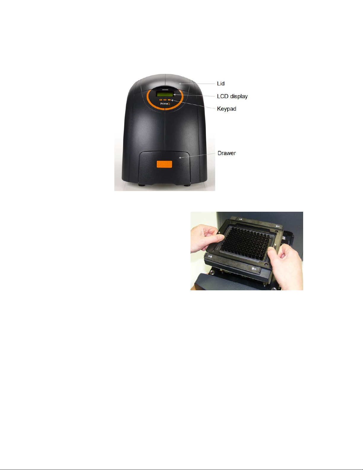
1.10.1 PrimeQ front view
1.10.2 Insert the block
Push firmly on the front of the drawer to open it
and insert the block.
Slide the quick release handles in the
direction shown on the top to the unlock
position.
Lift the block assembly into the unit. Never
lift or carry the block by one side, always
use both sides (or support the block from
underneath).
Ensure the block is fully engaged by
pushing all four corners of the block down
into the carrier.
Slide the quick release handles in the opposite direction to lock the block assembly in
position.
Push the drawer back into the unit.
1.10.3 Fuses
Ensure that the correct fuses are fitted for your voltage supply.
Fuses should only be changed by a competent person with training if necessary.
For voltages from 110 V to 130 V, use T10A fuses only.
23

1.10.4 Connections on the back of the unit
There are two cable connections: the mains power switch and
the USB socket located on the rear of the PrimeQ.
A. USB computer connection. Plug the USB lead into the
socket and connect the other end to your computer. The
lead must be less than 2 meters in length (the lead
supplied with the instrument is correct).
B. Power switch.
C. Fuses
D. Power connection. Ensure that the switch is in the off, O,
position. Plug the mains cable into the power socket.
When PrimeQ is sited in the correct position and all the
connections have been made, turn the switch to the on (I)
position on the PrimeQ.
24

1.11 Technical Specification
Thermal cycler
Block Format: 96 x 0.2ml well low-profile micro tube plate
Block Specification: 8 x Peltier block employing quad circuit technology
Block Uniformity at 50ºC: < ± 0.25ºC
Maximum Heating Ramp Rate: 2.2ºC/sec
Temperature Range: 4ºC to 98ºC
Sample Volume: 15µl to 50µl
Heated Lid: Adjustable between 100ºC and 115ºC or off
Optical detection system
Excitation Source: White LED
Detector: Photon counting photo multiplier tube (PMT)
Multiplex Dye Detection: Up to four dyes per reaction tube
to enhance performance
User Selected Filters: Maximum of four paired excitation/emission filter
Fluorescence Excitation Range: 470nm to 650nm
Fluorescence Detection Range: 500nm to 710nm
Dynamic Range: At least nine orders of magnitude from starting
Sensitivity: 1.0nM fluorescein in a 20µl sample
Dimensions
Weight: 25kg
Size and Footprint: 420mm x 528mm x 518mm (W x H x D)
Power Supply: 100V to 230V, 50/60Hz
Input Power: 715W
IP code: IP30
cartridges suitable for use with currently available
dyes
copy number.
Single initial template copy detection*
* Assay dependent
25

Computer requirements (Not Supplied)
The following are the recommended minimum PC specifications required for running PrimeQ:
CPU: Core 2 Duo or equivalent
Memory: 2Gb DDR RAM as a minimum
Storage: 40Gb DMA hard drive
Display: 1024 x 768 resolution minimum, 17 inch digital
monitor recommended.
Drive: DVD/CD-RW drive
®
Operating System: Microsoft
Windows
Connections: USB
Windows® XP Professional SP3 or later,
®
Vista, Windows® 7
Also useful:
Sound: Built-in sound, video and LAN facilities
Internet: Ethernet connection
Software: Internet Explorer, Microsoft® Office
PC must be operated in ‘always on’ mode, no hibernation or sleep mode allowed.
1.12 Working conditions
PrimeQ is designed to work safely under the following conditions:
Ambient temperature range: 5°C to 40°C
Humidity: Up to 80% relative humidity, non-condensing.
Notes:
The control specifications are quoted at an ambient temperature of 20°C.
The specification may deteriorate outside an ambient temperature range of 18°C to 30°C.
Warning:
The unit may be damaged if used in an ambient temperature above 40°C.
1.13 Guarantee
Please read this important GUARANTEE information.
Notwithstanding the description and specification(s) of the units contained in the Operator Guide,
Techne hereby reserves the right to make such changes as it sees fit to the units or to any
component of the units.
This Guide has been prepared solely for the convenience of Techne customers and nothing in this
Manual shall be taken as a warranty, condition or representation concerning the description,
merchantability, fitness for purpose or otherwise of the units or components.
The PrimeQ unit is guaranteed for a period of 2 years from the date of purchase.
26

Within these periods we undertake to supply replacements free of charge for parts which may on
examination prove to be defective, provided that the defect is not the result of misuse, accident or
negligence.
On all correspondence, please quote the Serial Number in full and/or the Sales Order Number.
Any instrument requiring service under this guarantee should be taken to the supplier through
whom it was purchased, or, in the case of difficulty, it should be carefully packed in its original
packing and consigned, carriage paid, to us. Techne takes no responsibility for returned goods
damaged in transit.
Returned goods will not be processed without a Returns Authorization Number.
Call the Service Department on +44 (0)1785 810475 or +1 609 589 2560 in the US for a Returns
Authorization Number.
Please write the Returns Authorization Number on the outside of any packing and ensure that a
copy of a Decontamination Certificate is visible.
Please register online or complete and return the Registration Card to the address on the card.
Returning the card or registering will help us to contact you with new information about Techne
products and product up-dates thus improving our service to you.
WARRANTY
Void
IF BROKEN
The Guarantee will be rendered invalid if any of the small labels shown
opposite are broken or missing when the unit arrives at the supplier’s under
any claim for warranty repairs.
27
1.14 Installing the application software
Always set your PC or laptop from which you are running PrimeQ so that standby is switched OFF.
This can easily be achieved through the control panel or:
Right click on the desktop and select Properties.
Select the Screen Saver tab and click on the Power button.
Activate the power scheme entitled Always On from the drop down menu and click Apply.
You may need to restart your computer.
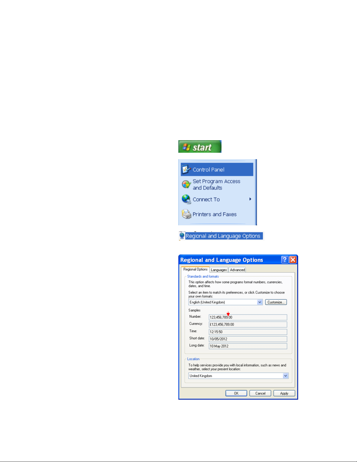
1.14.1 Set the decimal symbol to‘.’
Before installing this software please ensure that the decimal symbol on the computer is set to ‘.’.
If it is not then follow these instructions:
Click on the Start button:
Go to Control Panel:
Select Regional and Language Options:
Ensure the decimal in the number section
is set to a ‘.’
28
1.14.2 Loading Quansoft onto the PC
To install the Quansoft software onto the PC, follow these five basic steps:
1. Turn on the PC and log on as a user having administrator rights (to be able to install software).
2. Insert the Quansoft CD into the CD-ROM drive and wait for the auto-run function to
automatically start the setup (should auto-run fail to start, then the CD must be opened from
Explorer and the setup program (Setup.exe) initiated manually by double-clicking).
3. Click on the Install button and wait for the installation to complete. Quansoft files will
automatically be installed to C:\Programs\Techne\Quansoft. If you wish to change the
destination click the Browse button and choose accordingly. You will also be given the option
of creating a shortcut icon from the desktop for easy access.
4. Remove the disk from the drive.
5. Restart the computer, log on and then launch Quansoft from the Programs menu or via the
shortcut icon on the desktop.
The software can be easily uninstalled from the computer:
simply access the PC Control panel, click on Add/remove
programs and then select Quansoft.
If upgrading from one release of Quansoft to another, then
the previous release should first be uninstalled as described.
Note: the Release number should not be confused with the
version numbers which relate to each of the Quansoft editors.
Techne
Techne
Techne
Bibby Scientific
Bibby Scientific
Bibby Scientific
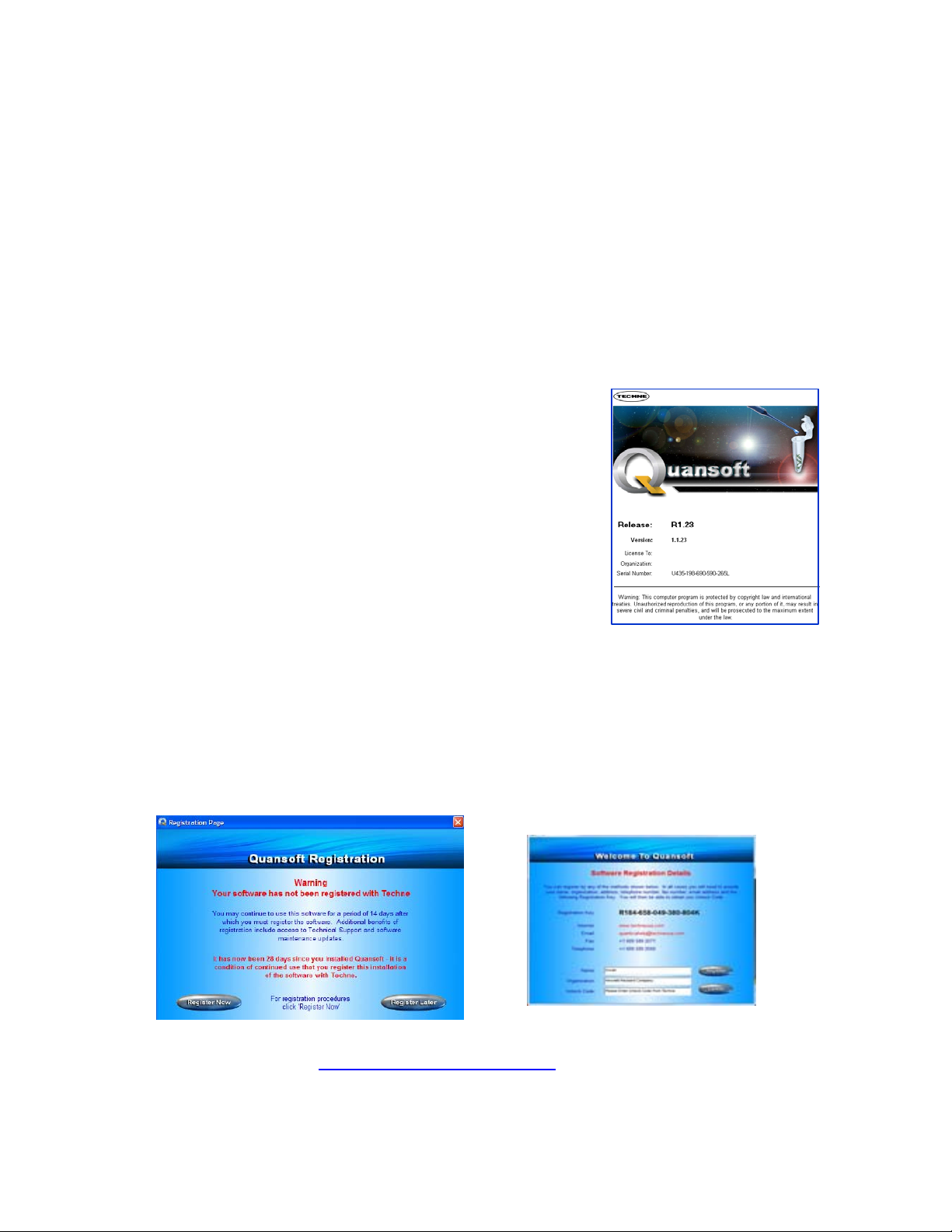
1.14.3 Registering the software
A registration welcome screen will appear when launching Quansoft for the first time. By
registering your software with Techne, you will be eligible for technical support and software
updates posted on the Techne website. However, the software can still be used for a 28-day trial
period without registration – simply click Register Later and the prompt screen will appear next
time the software is opened. On pressing Register Now, a form will be displayed requiring the
following fields to be completed: name, organization, unlock code and the instrument serial
number, should one be connected.
The unlock code can be obtained in one of three ways:
1. Internet: Clicking on www.techneusa.com/PrimeQregister in the registration panel, you will be
taken directly to the PrimeQ registration page.
a. Enter your details as listed on the screen.
29

b. An unlock code will be e-mailed to you within one working day.
Ensure you are online before attempting to do this.
2. E-mail: PrimeQhelp@bibby-scientific.com or PrimeQHelp@techneusa.com.
Send an email complete with details of your name, company or institution, mailing address, email address, telephone number, instrument and block serial number (if you have a PrimeQ)
together with the unique registration number.
Exit the registration procedure by pressing ’cancel’ and return when the unlock code has been
returned by email.
3. Phone: Provide us with your details and registration number by telephoning: +44 (0)1785
810433.
1.14.4 Software upgrades
Development of the PrimeQ control and analysis software is an ongoing process. To check your
version number, click ‘Help/About Quansoft’ and a splash screen displaying the current details will
appear.
Check the Techne websites at www.techne.com or www.techneusa.com for the most current
software updates. These updates can be downloaded free of charge for registered users.
30

1.15 Using the LCD control panel
1.15.1 Function keys
PrimeQ is controlled primarily from the PC using the application software, although some basic
functions can be performed via the LCD screen located on the front of the instrument.
The display indicates the instrument name, current status and basic information about any
experiment currently running such as its progression. The keypad has three function buttons:
Start/Pause: Starts the run or pauses if already running.
Stop: Stops the current run. The screen will ask for confirmation of the stop
command. This button can be deactivated from Quansoft to guard against
accidental stoppage.
ii
Info: Information about the program currently running on the unit can be obtained
at any time during the run.
1.15.2 Power up screen
The screen is a 20 character, four row LCD. There is a four button keypad.
1.15.3 Beeper
A beeper is used typically to:
Inform the user of any error made when interacting with the instrument (such as an invalid
key press).
Indicate a change of state of the instrument during a run (such as run completed).
31

1.15.4 Before you start
r
r
r
Check that:
1. All cables are connected between the instrument and PC.
2. All power cables are plugged in and comply with safety standards.
3. The Quansoft software has been installed on the PC.
1.15.5 Start-up procedure
1. Turn on the power to PrimeQ by pressing the switch at the back of the instrument. A welcome
beep can be heard.
2. Turn on the PC and wait for Windows to boot up.
3. Log in under your user name.
4. Double-click the Quansoft icon on the desktop to launch the software.
PrimeQ is now ready for use.
1.16 Installing the filter cartridges
1.16.1 The role of the filter cartridge
The role of the filter cartridge is to control the excitation and emission wavelengths of light using
filters and a dichroic mirror.
The excitation filter transmits only the wavelength of the light source that excites the
fluorophore.
The emission filter transmits only the wavelength of the light produced by the fluorescence
of the sample.
To and from fibre bundle
To and from fiber bundle
Dichroic mirro
Dichroic mirro
From light source
From light source
Excitation
Excitation
To detector
To detector
Emission filte
Emission
1. White light from the LED light source enters the cartridge and is separated by the excitation
filter.
2. Light of the desired wavelength is then turned 90° by a dichroic mirror and directed to the wells
via the fibre optic bundle.
3. Emitted light produced by the excited fluorophores is transmitted via the fibre optic bundle,
straight through the dichroic mirror and filtered by the emission filter such that only light at the
correct emission wavelength is allowed through.
4. Emitted light is passed on to the photo-multiplier tube (PMT) for detection.
The filters provided with the system are high-quality components with special anti-reflective
coatings. As with all filters, they will degrade over time, especially in climates with higher humidity
levels. This will ultimately lead to degradation in the instrument performance such that the
purchase of replacement filter cartridges is required (see section 5.6). Filters should last at least
three years, possibly as long as five depending on the frequency of use and conditions.
32

1.16.2 Filter cartridge care instructions
The filter cartridges must be handled with special care.
Only lift them from the foam in the box by the sides of the cartridges.
Avoid touching the filters.
Loose particles should be removed with a bulb puffer or filtered, pressurized air cleaner. If
necessary, gently wipe the surface using 100% alcohol and optical wipes; use a clean optical wipe
each cleaning motion.
1.16.3 Filter cartridge installation
The filter cartridges are positioned in a carousel with each cartridge having an identification label
visible from the access door. Installing filter cartridges into the carousel is a relatively simple
procedure that can be carried out by the user.
In Quansoft, access the filter settings screen by clicking on the Cartridge icon located on
the navigation bar of the Home Page (found under the Maintenance tab).
This will bring up the Cartridge Access and Editing screen. An instrument must be connected for
this screen to be displayed.
Cartridge position: Colour-coded for ease of identification.
Add/Remove/Edit/Replace: Launches a wizard which leads the user through the requested
procedure.
33

Excitation/emission wavelengths: As defined in the Add Cartridge settings box.
Dye name: Each cartridge can be assigned up to four different dye names of the user’s
choice (e.g. FAM, fluorescein, SYBR
®
Green etc.).
1.16.4 Adding a filter cartridge
In the Access and Editing screen of the Filter Wizard, click the Add button next to the
appropriate filter. The Add Cartridge screen will appear.
Set the wavelengths and bandwidths for the excitation and emission filters.
This information can be found on the side of the filter cartridge.
These filter details become the filter ID such that the fluorophores are viewed or chosen by the dye
name e.g. FAM or Cy5. The input table can hold details for the four filter positions of the carousel.
Click Next.
A screen appears prompting the user to perform a five-step procedure.
1. Lift the top lid of the PrimeQ.
2. Lift the cartridge/carousel cover.
3. Insert the cartridge and ensure that the magnets
engage to hold it in place; you will hear a “click” as
the magnets engage. It is important that the
cartridges are fitted correctly.
4. Close both lids.
5. Once the cartridges have been installed in the unit, it
is the user’s responsibility to assign filter descriptions
so that the application software knows what type of
filter is located in which position of the carousel.
34

1.16.5 Assigning filter descriptions in Quansoft
Once the cartridge has been fitted into the cartridge carousel, the system will check for the
presence of a new cartridge and then ask the user for the Dye Names. Up to four names can be
assigned to any given filter cartridge and the colour coding can be changed by clicking on the
Colour icon. The colour chosen here will be the colour of the dot representing the read points on
the thermal profile graph.
The assigned cartridge will now be available for use in the Program Editor (see section 3.4.3). It
is represented by the icon colour chosen during installation, although the colour can be changed
by double-clicking the icon in the read settings box. The user can choose to select a cartridge by
name or by wavelength. Simply click the Select by Name/Wavelength button to select which filter
to use.
1.16.6 Editing filter descriptions
Clicking the Edit button in the Cartridge Access & Editing screen brings up the settings boxes so
that it is possible to change the wavelength, bandwidth, name or icon colour for the filter. Perform
the steps in the same way as when adding a cartridge.
1.16.7 Removing a filter cartridge
If a cartridge is placed into the filter carousel without being installed via the software, a message
will warn the user of the presence of an illegal cartridge and the cartridge will be unavailable for
use. To remove this or any other cartridge, use the following procedure:
In the Access and Editing screen of the Filter Wizard, click Remove next to the appropriate
filter.
Click Yes to confirm the procedure and the Remove Cartridge screen will appear.
Follow the procedure as shown and click Finish to complete.
35

A message will appear informing the user to Please wait – checking cartridge status.
If the removal was performed correctly, the Cartridge Access and Editing table will be updated to
display “Not Fitted” next to the slot from which the cartridge was removed.
The table below gives details of the PrimeQ filter cartridges.
Filter
cartridge
FC01 460 500 FAM multiplex
FC02 485 520 FAM/SYBR®
FC03 530 560 HEX/TET/JOE/VIC/Yakima Yellow
FC04 580 615 ROX
FC05 640 685 Cy5/Quasar® 670
Excitation
wavelength (nm)
Emission
wavelength (nm)
Suitable dyes
1.16.8 Points to remember
Filter descriptions are stored in the instrument memory and do not need to be re-entered if
the connected instrument is changed to a different PC. Filter descriptions are uploaded from
the instrument when Quansoft is opened.
Changing the filter cartridge between experiments can only be carried out via the software –
it cannot be performed manually.
It is critically important that the correct excitation and emission filters are in the assigned
position of the carousel.
During multiplexing you must choose two fluorophores with different excitation and emission
wavelengths and measure the fluorescence with different filter cartridges.
Avoid combinations of fluorophores with overlapping spectra.
It is possible for some fluorophores to appear more than once on the dye list because more
than one filter pair could be used for its measurement. In this case, select the correct filter
by its wavelength properties.
1.17 Changing the instrument name
All PrimeQ units are shipped with the name “PrimeQ” stored in the instrument’s software. This can
be changed to a more appropriate name as required.
To change the instrument name, click on the Maintenance icon on the navigation bar. Then
click on the Instruments icon. The default supervisor password is techne – we suggest you
change this as soon as possible by clicking on the Security icon. Please ensure that you
keep a record of the password, as without it you will not be able to access these functions.
36

On the instrument screen, click on Change, type in the new name and then click OK.
Once the name has been changed you need to switch off the instrument before the new name can
appear on the LCD screen and take effect.
The maintenance screen also gives instrument-specific details including serial number, unique ID
and block cycle count. It also shows block constant (calibration) settings.
37

1.18 LED power settings
The LED light source has variable power settings. This prevents PMT blinding and brings
fluorescence into its linear range for certain applications. The role of this option is to cut down
excess light from the LED source in high fluorescence applications. The three power options are:
Low (50mA), Medium (100mA), and High (200mA).
The power level is specified by the user when programming the PCR in the application software
(at the same time as specifying the fluorophore filter); the default setting is Medium. The three set
power levels are not user-adjustable.
1.19 Inserting a plate
To insert a plate, push the orange panel to release the latch, and open the drawer by sliding
it towards you.
To close the drawer push it home until the latch clicks and the drawer stays shut.
1.19.1 Inserting a previously run plate
Users should note that when the thermal cycler plates are heated, the plastic may tend to distort
slightly. This means that if the plate is removed from the block then either returned or transferred
to another block, the fit can be poor. If returning or transferring a plate is unavoidable then the
following procedure is recommended to improve the fit:
If a heat seal has been used, place the plate in the heat-sealer and seal the plate for 3-4
seconds; rotate the plate 180 degrees; seal the plate for 3-4 seconds.
Insert the plate in the block and close the drawer.
1.19.2 Running a plate
Perform the loading procedure on the prepared plate following the instruction given when the
experimental run is started in the Quansoft operating software.
38

1.20 After use
When the samples have finished thermal cycling, remember that parts of the unit,
such as the tubes, blocks and associated accessories, may be very hot. Take the
precautions listed earlier.
Después de su uso
Cuando haya finalizado el calentamiento de muestras, recuerde que las piezas del equipo, tales
como tubos, bloques y demás accesorios, pueden estar muy calientes. Tome las precauciones
mencionadas anteriormente.
Après utilisation
Lorsque vous avez fini de chauffer les échantillons, n’oubliez pas que certaines parties de
l’appareil - les éprouvettes, leurs supports et autres accessoires - risquent d’être très chaudes. Il
est donc recommandé de toujours prendre les précautions citées plus haut.
39

40

2 Getting started
Introduction to PrimeQ and real-time PCR
About this chapter
This chapter gives a description of PrimeQ together with a basic
introduction to real-time PCR. It also provides examples of some of
the fluorescent chemistries that can be used with PrimeQ.
Forward primer
Forward primer
Forward primer
Forward primer
AGCTTAGGCCTAACCG
AGCTTAGGCCTAACCG
AGCTTAGGCCTAACCG
AGCTTAGGCCTAACCG
5’ 3’
5’ 3’
5’ 3’
5’ 3’
TCGAATCCGGATTGGCAGCTAAGGTTTCCAGATTCCAAATGCGCTA
TCGAATCCGGATTGGCAGCTAAGGTTTCCAGATTCCAAATGCGCTA
TCGAATCCGGATTGGCAGCTAAGGTTTCCAGATTCCAAATGCGCTA
TCGAATCCGGATTGGCAGCTAAGGTTTCCAGATTCCAAATGCGCTA
AGCTTAGGCCTAACCGTCGATTCCAAAGGTCTAAGGTTTACGCGAT
AGCTTAGGCCTAACCGTCGATTCCAAAGGTCTAAGGTTTACGCGAT
AGCTTAGGCCTAACCGTCGATTCCAAAGGTCTAAGGTTTACGCGAT
AGCTTAGGCCTAACCGTCGATTCCAAAGGTCTAAGGTTTACGCGAT
3’
3’
3’
3’
GATTCCAAATGCGCTA
GATTCCAAATGCGCTA
GATTCCAAATGCGCTA
GATTCCAAATGCGCTA
Reverse primer
Reverse primer
Reverse primer
Reverse primer
5’
5’
5’
5’
41

42

2.1 Introduction to PrimeQ
2.1.1 Principle of a real-time PCR instrument
A real-time polymerase chain reaction (PCR) system performs three main functions:
Cycles the PCR reagents through the specified temperature profile using a specially
designed thermal block.
Excites the fluorescent dye at the appropriate wavelength and at the appropriate point(s) in
the PCR program.
Detects the emitted fluorescence in each well during the specified read point - this
information is then fed back to the application software for analysis.
2.1.2 Principle of PrimeQ
PrimeQ is a real-time PCR system that combines a thermal cycler, solid state white light excitation
source and a highly sensitive fluorescence detection system all within the convenience of a
standard 96-well format. Combined with Quansoft, the system’s powerful analysis application
software, real-time quantification and analysis is made fast, easy and accurate. PrimeQ has been
designed with the advantage of an open chemistry format that gives the user full flexibility in the
methods and research they wish to pursue. The system is able to detect as little as 1.0nM
fluorescein and achieve a dynamic range of at least nine orders of magnitude†.
In line with the real-time principle, PrimeQ measures the amplification of DNA via a proportional
increase in fluorescence which is fed back to the application software. This allows the software to
calculate the starting DNA concentration by comparison to a set of standards. The system is
capable of measuring up to four different fluorophores per well in real time, thus opening up the
possibility of multiplex experiments, where multiple dyes are conveniently used within the same
reaction.
The time taken for PrimeQ to read a plate can be adjusted by varying the integration time. Read
times can be programmed from 250ms/well integration time (30 seconds/ 96-well plate) down to
just 50ms/well (10 seconds/plate) for brighter fluorophores. The default integration time is
150ms/well, which gives a read time of around 20 seconds for a 96 well plate.
2.1.3 Applications of PrimeQ
1. Quantitative real-time PCR: Monitoring the accumulation of a PCR product as the run
progresses by detecting the increase in fluorescence. Data collection in the early exponential
phase of the PCR allows the Quansoft software to accurately calculate initial template
quantities.
2. Qualitative (end-point) PCR: At the end of a run, the instrument is programmed to read the
plate a user-defined number of times for as many fluorophores as present in the samples. The
result indicates positive or negative amplification and the data can be analysed in a number of
ways to give a qualitative result.
3. Dissociation point determination: Samples are slowly heated from the annealing
temperature (typically 50 to 65°C) up to the denaturation temperature (~95°C) in small steps.
Fluorescence is measured at each step to determine the amount of dye bound to the dsDNA.
The point at which the two strands separate is associated with a decrease in the fluorescence
signal as the dye can no longer intercalate with the two strands. It is therefore possible to
determine the temperature at which 50% of the double-stranded DNA is dissociated (Tm).
Since the dissociation temperature of a DNA product is characteristic of the GC content, length
and sequence, the Tm can be a useful tool in product identification.
† The dynamic range is assay dependent.
43

2.2 Introduction to Real-time PCR
2.2.1 PCR
PCR is a powerful biochemical technique that has revolutionised biological research by allowing
minute amounts of DNA to be amplified millions of times in just a few hours. PCR allows the
selective amplification of a ‘target’ region of DNA lying between two specific DNA sequences
(primers). The DNA sequence lying between these primers does not need to be known, therefore
PCR allows researchers to amplify target DNA with relative ease and reproducibility.
The technique exploits the 5’ to 3’ polymerase activity of the enzyme Taq DNA polymerase
isolated from the thermophilic bacterium Thermus aquaticus. Once the primer binds to the
complementary region of the single-stranded target, the enzyme will catalyse the extension of
DNA to produce a complimentary second strand.
Forward primer
Forward primer
Forward primer
Forward primer
AGCTTAGGCCTAACCG
AGCTTAGGCCTAACCG
AGCTTAGGCCTAACCG
AGCTTAGGCCTAACCG
5’ 3’
5’ 3’
5’ 3’
5’ 3’
TCGAATCCGGATTGGCAGCTAAGGTTTCCAGATTCCAAATGCGCTA
TCGAATCCGGATTGGCAGCTAAGGTTTCCAGATTCCAAATGCGCTA
TCGAATCCGGATTGGCAGCTAAGGTTTCCAGATTCCAAATGCGCTA
TCGAATCCGGATTGGCAGCTAAGGTTTCCAGATTCCAAATGCGCTA
AGCTTAGGCCTAACCGTCGATTCCAAAGGTCTAAGGTTTACGCGAT
AGCTTAGGCCTAACCGTCGATTCCAAAGGTCTAAGGTTTACGCGAT
AGCTTAGGCCTAACCGTCGATTCCAAAGGTCTAAGGTTTACGCGAT
AGCTTAGGCCTAACCGTCGATTCCAAAGGTCTAAGGTTTACGCGAT
3’
3’
3’
3’
GATTCCAAATGCGCTA
GATTCCAAATGCGCTA
GATTCCAAATGCGCTA
GATTCCAAATGCGCTA
Reverse primer
Reverse primer
Reverse primer
Reverse primer
The classical PCR protocol consists of three temperature steps:
1. Denaturation (at 95°C): In its normal state, DNA
consists of two strands made up of complementary
bases. These strands need to be separated before
the PCR can progress. The first temperature step
is therefore designed to dissociate, or denature,
these two strands.
2. Annealing (typically between 55°C and 65°C):
This temperature step allows annealing of the
primers to complementary sequences on the
template DNA. The temperature will vary
according to the primer characteristics such as GC
content, length and sequence.
3. Extension (72°C): When the primers have
annealed to the complementary single-stranded
DNA, the enzyme Taq DNA polymerase extends
the DNA using its 5’ to 3’ polymerase activity. The
optimal temperature for this enzyme is 72°C.
This results in the production of two new copies of the target DNA which, assuming optimal
conditions, can be amplified exponentially by repeating steps 1 to 3.
The primers anneal to
complementary regions on
the template DNA.
5’
5’
5’
5’
2.2.2 Qualitative vs. real-time PCR
PCR quickly became an indispensable tool for scientists wanting to amplify and characterize
genetic material. However it has one major limitation in that the results are qualitative i.e. it can
determine if a target is present but not the amount. The traditional approach to quantification was
to compare known sample concentrations of starting DNA with unknown samples cycled at a
range of concentrations and cycle numbers. The problems associated with this ‘semi-quantitative’
approach are many, including the expense of multiple PCR runs, the increased risk of
contamination through the need for downstream processing of samples and the fact that end-point
measurements have a tendency to vary between replicates. As such, the very accuracy of the
post-run method of measurement is put into question. However, real-time PCR or quantitative
44

PCR (qPCR) extends the usefulness of the technology by permitting the reliable determination of
starting DNA template.
2.2.3 Real-time PCR on PrimeQ
Real-time PCR overcomes the limitations associated with the traditional methods by using
fluorescence labelling in conjunction with specialized amplification and detection systems to
quantify the amount of product being amplified during the PCR process. The fact that downstream
processing is eliminated saves both time and money while reducing the risk of contamination.
Further savings are to be found with the need for reduced replicates and that multiple reactions
can be combined within the same tube using different reporter dyes. However, the most notable
advantage over conventional approaches has to be its superiority in terms of accuracy and
sensitivity. As a result, this method has become a widely useful tool for the quantification of
messenger RNA or DNA levels in a wide range of biological samples.
PrimeQ provides a flexible approach to experiment setup by supporting real-time experiments for
monitoring the accumulation of PCR products during thermal cycling as well as end-point assays.
Quantitative PCR: The advantage of this approach is that amplification of the accumulated
product is measured in the early exponential phase of the reaction at a point when the
amplified product can accurately reflect the starting DNA or RNA levels. By the end of the
experiment, reagents could be limiting which may mean that small differences in the PCR
performance are magnified. Additional benefits of this approach are its high sensitivity and
wide dynamic range. PrimeQ can measure to a sensitivity level of 1.0nM fluorescein and
with a dynamic range of at least nine orders of magnitude.
End-point: This approach detects the presence or absence of an amplified product,
providing a qualitative positive or negative result. This approach can bring added flexibility to
the laboratory, allowing samples that have been run in a different thermal cycler to be
quickly screened for the presence of a PCR product by using PrimeQ as a plate reader.
In both approaches, the amount of product present in each reaction tube is visualized using
fluorescent reporter dyes.
2.3 Overview of fluorescent chemistries
An extremely sensitive system is required for the accurate visualization of small amounts of PCR
products. The conventional approach has been to use radioactivity, which although offering good
sensitivity, has obvious disadvantages in terms of safety and environmental risk. Fluorescence has
now taken over as the chemistry of choice due to its sensitivity, safety and the excellent flexibility it
lends to experimental setup.
Fluorescence is a molecular phenomenon in which a substance absorbs energy in the form of
light, causing it to first become excited and then to emit part of this absorbed energy as light of
another colour. This light will be of a lower energy and therefore a longer wavelength (λ) of that
absorbed.
Schematic representation
of fluorescence.
When considering which fluorescent chemistry to use on PrimeQ, there are two main options:
fluorescence-labelled probes that bind specifically to the target of interest or intercalating dyes that
bind between the two strands of double-stranded DNA. The fluorescence signal seen when the
45

dye is excited at the appropriate wavelength should be proportional to the quantity of target DNA
present. For each type of fluorescent chemistry, the fluorophore will emit a fluorescent light that is
characteristic of the fluorophore used. A range of spectrally distinct fluorophores are commercially
available, introducing the possibility of quantifying multiple targets with different probes in the
same reaction well, otherwise known as multiplexing.
2.3.1 Intercalating dyes
Intercalating dyes bind to the minor groove of double-stranded DNA (dsDNA) producing up to a
thousand-fold increase in fluorescence. Common examples include SYBR
®
Green I, EvaGreen®
and BRYT™Green. As these dyes bind all double-stranded PCR products, this is a universal
chemistry with the major advantage of not requiring the use of a fluorescently labelled probe. As
such, it is a relatively inexpensive approach and one that is ideal as a screening tool prior to probe
manufacture. However, these advantages bring their own disadvantages in that the ability to bind
all dsDNA means that both specific and non-specific PCR products, including primer-dimers, will
be reported.
The signal attributable to each PCR product can however be determined by dissociation curve
analysis, a technique that distinguishes PCR products on the basis of melting temperature (Tm).
PCR products of different lengths with different GC contents melt or dissociate at different specific
temperatures. Dissociation curve analysis thus allows the user, via the specific Tm, to establish
that the correct piece of DNA has been amplified. As only a single dye is used to detect all the
products, the chemistry is not open to multiplexing i.e. detection of multiple products.
Mode of action of SYBR
®
Green I:
When the DNA strands are
dissociated, the dye does not bind or
fluoresce.
®
SYBR
Green I binds non-specifically
to dsDNA. When excited, the emitted
fluorescence is relative to the amount
of dsDNA present.
The fluorescence will drop when the
strands start to dissociate. The
temperature at which 50% of the DNA
is single stranded is the Tm. Since the
Tm is influenced by GC content,
length and sequence, it will be
indicative of the identity of a PCR
product.
2.3.2 Fluorescent labelled probes
This approach is used when the most accurate quantification of PCR products is required or for
when there is more than one target in the reaction tube. Using dye-labelled oligonucleotides that
contain a region complimentary to the target sequence to be amplified, provides advantages in
terms of high specificity and low background. At the same time, the signal is also ensured to be
proportional to the amplified product and not the mass or the length. This chemistry is also
multiplex-compatible such that different ‘coloured’ dyes can be used to report different targets in
the same reaction well. Common examples of fluorescent probe chemistries are detailed below.
2.3.2.1 Hydrolysis probes
This chemistry exploits the 5’ nuclease activity of Taq DNA polymerase to cleave a probe during
PCR. The probes are designed as oligonucleotides that are complementary to a region of the
target located between the upstream and downstream primer binding sites. The probe contains a
fluorophore at the 5’ end and a quencher at the 3’ end; the close proximity of which means that
fluorescence is quenched prior to amplification due to the action of the quencher on the
fluorophore. The quencher absorbs the light emitted by the fluorophore with itself emitting either no
46
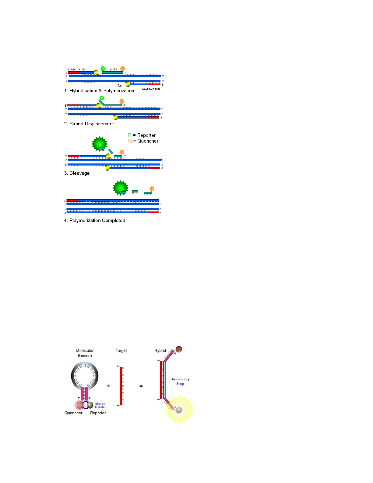
fluorescence signal or fluorescence at a longer wavelength which is not detected. The 5’
fluorophore is often called the reporter.
Mode of action of hydrolysis probes:
During the PCR, as the DNA polymerase extends the
upstream (forward) primer, it encounters the bound
probe.
The 5’ to 3’ exonuclease activity of the polymerase
cleaves the probe, releasing the fluorophore into
solution, where it is able to fluoresce.
The probe is blocked at the 3’ end to prevent
extension by the polymerase.
Each cycle of the PCR releases more fluorophore
such that the amount of fluorescence in any given
cycle should be proportional to the amount of specific
product present at any given time.
A particular advantage of the hydrolysis probe technology, aside of the specificity and sensitivity
afforded by all the fluorescent probe chemistries, is that the signal accumulation is irreversible.
Once a probe is cleaved, the quencher is permanently separated from dye and this is reflected in
the signal accordingly.
2.3.3 Molecular Beacons
As with the hydrolysis probe technology, molecular beacons use fluorophore/quencher pairs in
their mode of action. When free in solution, molecular beacons assume a hairpin structure that
brings the end-bound fluorophore and quencher into close proximity thereby quenching the
fluorescent signal. The molecular beacon binds to the amplicon produced during the PCR at a
specific temperature when the beacon-target duplex is thermodynamically more stable than the
hairpin structure. Binding of the beacon to its target disrupts the hairpin, resulting in spatial
separation of the fluorophore from the quencher and allowing it to fluoresce. This increase in
fluorescence is reversible as the beacon will dissociate at a higher temperature and close back to
a hairpin. The transition from hairpin to bound form is repeated each cycle.
Mode of action of molecular beacons:
When free in solution, molecular beacons
assume a hairpin-structure.
Binding of the beacon to its target
disrupts the hairpin, resulting in spatial
separation of the fluorophore from the
quencher and allowing it to fluoresce.
Molecular beacons combine the
specificity of a probe-based chemistry
with the versatility of a reversible binding
reaction.
47

2.4 System overview
PrimeQ is a real-time PCR unit into which the operator places a 96-well plate containing the
samples to be analysed. The unit is connected to a PC via the USB port on which the application
software (Quansoft) is run. The software allows the user to:
1. Create a PCR program defining dyes, read points, thermal cycling and analysis methods.
2. Run the program.
3. Analyse the fluorescence readings.
Thermal cycler:
Reader:
Software:
Consumable:
PrimeQ consists of three key parts: the optics module; a thermal cycler module and a scanning
module.
The specialized block cycles the temperature according to the predefined PCR program.
Allows fluorescence within each well of the plate to be read at
specified points during the PCR program. The reader excites the
samples at one wavelength and then detects the emitted fluorescence
at another.
The unit requires a PC installed with the application software,
Quansoft, for protocols to be defined and downloaded and for the
data to then be analysed.
The unit accommodates a low-profile 96-well plate (skirted or nonskirted) sealed with optical sealing film.
2.5 Optics module
The role of the optics module is to deliver excitation light into each well and measure the emitted
light at defined points in the PCR cycle. The light source is a solid state white light source with the
excitation and emission wavelengths controlled by a system of filters and a dichroic mirror housed
in the user-changeable filer cartridges. Four such filter cartridges can be accommodated at any
one time in the filter carousel.
48

2.5.1 The optical light path
r
r
r
Excitation light from the solid state white
light source (1) passes through a light
path and enters the filter cartridge. Only
light at the desired wavelength is allowed
to pass through the excitation filter (2).
The light is then reflected through 90° by
a dichroic mirror (3) and passed into a
fibre optic bundle (4). From there, the
light is directed into the wells of the
sample plate by the fibre optic bundle,
which excites the fluorophore present
specific to that wavelength.
Light emitted from the sample well
passes back up the fibre optic bundle,
straight through the dichroic mirror (3)
and then through the emission filter (5).
This filter blocks all wavelengths of light except the desired emission wavelength, which is passed
onto the photon counting photomultiplier tube (PMT) detector (6). Fluorescence levels are then
passed from the instrument to the PC via a USB connection where Quansoft analyses the data
using algorithms. Results can then be exported, printed or displayed graphically.
2.5.2 Filter cartridges
Each set, comprising excitation filter, emission filter and dichroic mirror, is mounted in a cartridge.
As detailed above, the role of the filter cartridge is to separate the excitation and emission spectra
appropriate for the fluorophore being used. The excitation filter transmits only those wavelengths
of light that excite the fluorophore, while the emission filter transmits only fluorescence produced
by the sample. The emission light is always of a longer wavelength (more to the red region of the
light spectrum) than the excitation light. As the filter carousel can hold multiple cartridges, the user
is able to change the filter to suit the chemistry being used – a procedure that is easily performed
from within the application software. Quansoft allows the user to install four filter cartridges in
PrimeQ.
To and from fibre bundle
To and from fiber bundle
2.5.3 Adjustable LED intensity
Dichroic mirro
Dichroic mirro
From light source
From light source
Excitation
Excitation
To detector
To detector
Emission filte
Emission
To allow the PrimeQ instrument to be optimized for the use of specific fluorophore combinations,
the user can choose to adjust the light intensity of the LED light source (50, 100 or 200mA
settings). This is useful for obtaining balanced results when using both bright and weak
chemistries/dyes in the same experiment.
2.6 Thermal cycling module
The thermal cycling module is an 8 Peltier thermal cycling block with quad circuit technology into
which the user places a low-profile 96-well sample plate. It is programmed from the application
software and is able to reach any temperature between 4° and 98°C.
49

PrimeQ’s thermal cycler block. accommodates a lowprofile 96-well plate.
Each block is internally calibrated so that if the block
is replaced, the temperature performance is
unchanged without having to recalibrate the
instrument
The thermal block fits into and can be accessed by
opening the PrimeQ sample drawer. This provides
the user with access to the block so that plates can
be loaded or unloaded or the block removed for
cleaning or replacement.
2.7 Scanning module
The scanning module delivers excitation light to the sample wells and then collects the emitted
light. It also plays a role in heating the top of the sample plate and in preventing sample
evaporation. It is made up of two basic components: the heated lid and the X-Y fibre optics.
Heated lid: This component is made up of a heated glass plate that comes into contact with
the top of the sample plate. Designed with a special optical coating, the heated glass plate
provides uniform heating at the uppermost surface of the sample plate and thereby prevents
sample loss due to evaporation and condensation. The heated lid also helps to hold the
sample plate flat, and by being located within a cover, it provides a light-tight chassis for the
X-Y fibre optics.
X-Y fibre optics: Excitation light is carried from the optics module to the sample wells
through a flexible fibre optic bundle. The X-Y mechanism scans each well in turn to
transport the light into and out of the sample wells. The same fibre optic bundle carries the
emitted light back from the well and into the optics module for delivery to the detector.
50

3 Quansoft
Using Quansoft
About this chapter
Accompanying PrimeQ is the intuitive, wizard-based software,
Quansoft. This chapter discusses the concepts behind this software
and looks at its application in the setting up and running of a realtime PCR experiment.
Read the first section for an overview of Quansoft in general terms
and a brief discussion of how the various parts fit together. The next
section helps the user to navigate around the software and reviews
its basic functions and commands. The final section gives a simple
step-by-step guide to the setting up, running and monitoring of a realtime PCR experiment.
51

52

3.1 Introducing Quansoft
PrimeQ is a real-time-PCR unit containing sophisticated thermal cycling and fluorescence
detection technology. The user interacts with the system via Quansoft, the user-friendly Windowsbased application software installed on a PC connected to the unit. The intuitive software allows
the user to perform three main functions:
1. Create a PCR program and define fluorescent reading points.
2. Run the program.
3. Detect and analyse the fluorescence readings.
At the heart of Quansoft lie the Editors; powerful software features that have been specially
designed to simplify setup, editing and customization of the experimental parameters. Plate layout,
thermal cycling program and analysis method parameters can all be conveniently accessed from
the Home page, with each Editor providing a flexible format and clear layout that makes viewing or
changing any aspect of the protocol simple and straightforward.
Quansoft Home page
By employing a series of user-friendly
windows, Quansoft enables any real-time PCR
experiment to be created with ease.
Experiment Editor
This powerful Quansoft feature acts much like
a shopping cart gathering together different
elements of an experiment. Using
combinations of plate layout and program
parameters, it offers the user a flexible
approach to the management of experiment
protocols.
Program Editor
Individual cycling steps/stages or ramps are
quickly added to build and display the thermal
program. Fluorescent reads can be added at
any step of a stage.
53

Plate Layout Editor
Within a matter of seconds, a 96-well
microplate can be assigned with various
sample types, including blanks, controls,
standards or user-defined samples, all of
which are colour-coded for ease of
identification.
Results Editor
Results for each stage of the program
containing fluorescent readings are shown on
individual tabs and can be analysed separately
using various analysis methods.
3.2 Software overview
The diagram below outlines the structure of Quansoft.
Home
Home
Page
Page
Analysis Wizard
Analysis Wizard
Program
Program
Editor
Editor
Click “Run” button
Click “Run” button
Real-time monitoring
Real-time monitoring
Analysis 2
Analysis 2
Analysis 1
Analysis 1
The starting point is the Home page, which provides easy access into the experiment setup. At the
heart is the Experiment Editor, whose role it is to act as a ‘shopping cart’ for the plate layout and
program elements. The Experiment Editor also incorporates the Analysis Wizard, which allows the
user to define the method of analysis and possible report options to be applied to the results postrun.
Experiment
Experiment
Editor
Editor
Run
Run
Screen
Screen
Results Editor
Results Editor
Report
Report
Experiment
Experiment
Analysis
Analysis
Plate Layout
Plate Layout
Editor
Editor
Layout
Layout
54

3.2.1 Home page
As shown in the schematic diagram above, the Quansoft Home page is the starting point for an
experiment, providing quick links to all of Quansoft’s most important features. Direct links into the
different editor functions allow the user to quickly create a new experiment, re-run a previous
experiment, edit a program or to analyse new or existing data. Basic maintenance and filter
changing functions can also be performed from links on the Home page.
3.2.2 The Editors
Quansoft consists of four editors: the Program Editor; the Plate Layout Editor; the Experiment
Editor and the Results Editor. These fit together to allow the creation, editing and analysis of a
real-time-PCR run. The first three, as shown above, are part of the experiment setup and allow the
user to set up the assay parameters. The Results Editor meanwhile, provides a platform by which
to view the results and to change or specify parameters for the analysis post-run and report
printout.
3.2.2.1 Experiment Editor
The Experiment Editor acts as a ‘shopping basket’ into which the components of the experiment
are gathered i.e. the program, plate layout and the analysis parameters. It provides a summary of
the setup thus acting as a gateway to browse, create or edit elements of the experiment. In
essence, the role of this editor is to simplify the management of the experiment protocols and to
provide a starting point for initiating a run on PrimeQ. Both the Plate Layout and Program Editors
can be accessed from the Experiment Editor, and when combined with a set of analysis
parameters, will produce a report of the results once the data has been collected. A copy of the
experiment can be stored as a template thus allowing the easy routine analysis of a specific
project. Experiments may also be shared between users with data from each user stored
individually as a Results file. These files are saved in a .qres format.
Quansoft’s Experiment Editor
acts as a ‘shopping basket’ for
the components of an
experiment.
3.2.2.2 Plate Layout Editor
As its name suggests, the Plate Layout Editor defines the plate layout for an experiment. The 96well plate can be left empty or assigned with blanks, controls, user-defined standards or test
samples, which are all colour-coded for ease of identification. If need be, the well layout can be set
up or changed after the run has completed and the data for analysis can be included/excluded
using the right click flagging function.
55

Quansoft’s Plate Layout Editor
is a flexible platform for defining
a plate layout.
In this editor, it is possible to set the name and value of samples used for a standard curve. When
placing standards in the layout, the user will be asked to fill in the value of each standard in the
Well Information table. To assign units to these standards, such as copies/well or ng DNA, options
are available in the drop-down list, or a custom unit can be defined. As with the experiment files, a
copy can be stored as a template saved in a .qpla format.
3.2.2.3 Program Editor
The Program Editor is the part of Quansoft where the user can define the temperatures, hold times
and reading parameters to be used in the PCR run. The minimum requirement in order to start a
run on PrimeQ is for the experiment to have a valid thermal cycling program – other settings such
as plate layout and analysis method can be defined and/or changed post-run. These files can be
saved to the Program Library in a .qprg format.
Quansoft’s Program Editor
provides a simple approach to
defining the thermal cycling
program and dye reads.
3.2.2.4 Results Editor
This editor displays the results data. Clicking on the Experiment tab allows analysis settings to be
redefined or report options to be changed. The role of this editor will be examined more closely in
Chapter 4.
56

Quansoft’s Results Editor
displays the results of the run,
which can be sent to report or
re-analysed with different
parameters.
3.3 Using Quansoft
3.3.1 Home page
The Quansoft Home page acts as a gateway to the software functions, providing quick and easy
links to both the Editors and their associated libraries. Other functions, such as basic instrument
maintenance, filter changing, and administrative tasks, can also be carried out from here.
57

3.3.2 Main screen
Shortcuts for experiment setup and data analysis:
Run an experiment: goes to the Experiment folder to select an experiment.
Create a new experiment: goes to the Experiment Editor from where the user
can create a new experiment or edit an existing one.
Create a new program: goes to the Program Editor from where the user can
create a new program or edit an existing one.
Create a new plate layout: goes to the Plate Layout Editor from where the user
can create a new layout or edit an existing one.
Analyse data: goes to the Results folder from where the user can open up the
results of an experiment in the Results Editor.
3.3.3 Navigation bar
Located on the left-hand side on the Home page, the navigation bar provides easy access to the
different editor libraries and the maintenance section of the software.
Home page icon:
Clicking the Home icon when in one of the libraries returns Quansoft back to the
Home page.
Library icons:
Clicking the Program icon opens the Programs directory in the library folder. The
Program Editor will open if the New button is pressed.
Clicking on the Plate Layout icon opens the Layouts directory in the library
folder. The Plate Layout Editor will open if the New button is pressed.
Clicking the Experiment icon opens the Experiments directory in the library
folder. The Experiment Editor will open if the New button is pressed.
Clicking the Results icon opens the Results directory in the library folder. The
Results Editor will open if a results file is opened.
Maintenance icons:
58
Clicking the Filters icon opens the Cartridge Access and Editing screen to allow
the installation, changing and naming of filters using the Filter Wizard.

Clicking the Security icon allows customizing of the supervisor password
(required for the administrative functions which are accessed under the
Instrument icon).
Clicking the Instrument icon will allow the user to view instrument-specific details
including, for example, the instrument serial number and block cycle count. The
default supervisor password is techne - we suggest that you change this as soon
as possible. Please ensure that you keep a record of the password as without it
you will not be able to access these functions.
3.3.3.1 Library view
Clicking on the Libraries tab, the navigation bar will display icons for each library: Programs (.qprg
files), Plate Layouts (.qpla files), Experiments (.qexp files) and Results (.qres files). The contents
can be browsed and previewed in the pane in the lower half of the screen, and by opening it up in
the relevant editor (either by double-clicking the file or browsing from within the relevant editor),
the files can be edited and analysed with ease. The libraries can be navigated by moving up and
down the directory structure with users able to create folders and organize data in the usual way.
3.3.4 Title bar functions
Shortcuts to frequently used library functions are also found on Quansoft’s Title bar.
The Home button returns the software to the Home page where there are quick
links to the other functions.
The New button will open a blank editor window depending on which library has
been selected (inactive for the Results library).
The Delete button can be used to delete selected files or folders from a library.
59

The Up button allows the user to navigate back to a previous folder (used if the
directory structure has been turned off).
The View button will change the way the files are displayed in the file view pane
(detail, large/small icon, list views).
The following buttons are displayed on the Title bar when using one of Quansoft’s Editors:
The Finish button (Results Editor) saves the changes made and closes the
editor.
The Save button will open the Save As window, allowing the user to save the file
under a new name.
The Open button allows the user to browse and select files from a library.
3.3.5 Menu bar functions
Quansoft’s menu bar offers many of the functions found in a typical MS Windows application.
Click the Quansoft icon to move, maximize,
minimize or restore the screen.
Click on the menu bar options beneath the Quansoft icon for drop-down menus offering the
following functions:
File: Contains file manager commands. Click the
appropriate function to open, close, delete, re-name or to
check the properties of a particular file. Greyed-out
commands are disabled.
Edit: Contains functions for the cutting, copying or pasting
of selected text or graphics.
60

View: Allows the user to change the way the files appear in
the file view. Choose to display simply as icons or display
with further details such as file name and size.
Tools: Provides direct access into the editor of choice simply click on the editor name. The Change Quansoft
folder… command allows the user to change the
destination of any saved files. Quansoft will automatically
save all files to My Documents\Quansoft; change the
destination here if required.
Help: Off- and on-line resources. Click Quansoft Help
(short cut key F1) for access to this Operator guide, or click
on Techne on the Web to link to the Techne website.
Clicking on About Quansoft will bring up details about the
software including the version and serial number.
Registered users of Quansoft will be kept informed of
software updates.
3.3.6 Accessing the editors
The user can access the Quansoft editors by the following routes:
Home page: Click the round shortcut icons as discussed in section 3.3.2.
Menu bar: Go to Tools and click on the editor of choice.
Library files: Clicking on a library file will open up that file within the relevant editor. Either
browse a library file from the Home page or browse from within an editor.
New or Browse: Clicking on these buttons in the program or plate layout pane of the
Experiment or Results Editor opens up the relevant editor within. Files can then be browsed,
edited or created from new.
Start menu: Click on the Windows Start button in the bottom left hand corner. Choose All
Programs/Techne/Quansoft/Editors and then select the editor of choice.
61

3.4 Setting up an experiment
3.4.1 An Overview
Schematic diagram showing the options available for setting up an experiment on PrimeQ.
The icons in the blue boxes represent the shortcut buttons available from the Home page.
START 1: Choose to set up an entirely new experiment in the Experiment Editor, browse or edit
previously saved plate layout or program templates or else access the Plate Layout and Program
Editors direct from the Home page.
START 2: A previous experiment can be opened and run with no changes to the parameters or
results from a previous run can be analysed directly.
62

3.4.2 Creating a new experiment
From the Home page click on Create a New Experiment.
A blank experiment template will open in the Experiment Editor.
The Experiment Editor allows the user to perform three important functions:
Define a program,
Define a plate layout
Define an analysis method
Note: only the setting of a program is essential for a run to be performed; plate layout and analysis
method can both be defined after the run is complete.
The options for setting up individual experiment components are:
1. Program Setup:
a. From New
b. Browse an existing template
c. Edit the selected template
63

2. Plate Layout Setup:
a. From New
b. Browse an existing template.
c. Edit the selected template
3. Analysis Method Selection
This chapter will look at each of these functions in turn.
3.4.3 Setting up a program
The PCR program is defined using the top-left area of the Experiment Editor main screen:
There are three ways to define a PCR program:
Click this button when the program is to be defined entirely from new.
Click Browse to search the Program library files for existing templates.
Click to edit the selected program template
3.4.3.1 Define a new program
To create a new program, click the New button.
The Program Editor will open up within the Experiment Editor with a blank program screen.
64

Run information: The user can enter a user name and add any other comments relevant to
the program.
Instrument settings: User-defined settings for heated lid temperature, disabling of the
instrument buttons, plate type, sample volume and whether to read entire plate or include a
final hold in the PCR program.
Program file view: Displays the structure of the program thereby providing the user with a
clear view of the overall protocol.
Temperature profile: Provides a summary plot showing the temperature profile for each
cycle of the stage (or the complete program when viewing at the Program level).
3.4.3.2 Run information
Enter a user name and any comments in the appropriate text boxes (optional).
Clicking on the padlock icon to a locked position prevents the user from
accidentally saving over the existing file – to save the changes the user must
use the File menu Save As… option and save the file under a different name.
3.4.3.3 Instrument settings
Define the general instrument settings for the run.
65

Heated Lid: Default 105°C. Set a temperature (possible temperature range from 100°C to
115°C).
Wait For…: Set a ‘wait for’ time (i.e. the time to wait while the lid heats up before the block
thermal program begins, hrs:min:sec). Or click the button to wait until heated, the program
will then start as soon as the lid reaches the set temperature.
Read Whole Plate: Default ON. Click to Read only filled wells. This can be useful to
reduce the time taken to read the plate if only a partially filled plate is in use. Note: a plate
layout must be defined in order to read only the filled wells.
Instrument Buttons: Default enabled. Click to disable (prevents against accidental
stoppage of the instrument using the instrument buttons, so that the program can only be
controlled from within the software).
Plate Type: Default Clear. Scroll down to select a different plate colour.
Sample Volume: Default 20µl. Change as appropriate (max 50µl, min 15µl).
Final Hold: Default OFF. Activate by clicking. Set time and temperature as appropriate.
3.4.3.4 Program
A program is set up in a logical fashion whereby temperatures and hold times are defined for each
stage, as would be done on a typical thermal cycler. The major difference is that the user will tell
the instrument when to take a fluorescent reading and which filter cartridge(s) should be used.
Each stage of the Program is made up of temperature steps
cycled x number of times.
Click Add Stage to open a new stage and label it
accordingly.
Click Add Step to add the relevant temperature steps to
each stage.
Click Add Ramp to add a ramp read (melt stage, see
section 3.4.3.6).
Steps with a dye read are highlighted in red; a ramp read is
highlighted in blue.
Level 1: Program
Name the program if desired (the default is New Program) and set the instrument settings.
Level 2: Stage
Click Add Stage. On doing so, a new stage folder will appear in the file view:
66

The default name New Stage can be changed if required.
When a stage name is highlighted in the program file view, the stage parameters box in the centre
of the screen allows the general parameters for that stage to be defined.
Heated Lid: The default is to keep the heated lid temperature unchanged. To change, click
the button and a time and temperature setting box will appear adjacent (possible
temperature range from 100°C to 115°C).
Number of Cycles: Define how many times the stage should cycle (range between 1 and
99).
Do Not Pause: Default ON. If a pause is required after this stage then click on this button.
To delete or rename a stage, right click on the stage folder and select the appropriate command.
Alternatively, highlight the stage and select the appropriate command from the Tools menu in the
tool bar.
Level 3: Step
Click on Add Step to add a temperature step to a stage.
When a step is highlighted in the program file view, the step parameters box in the centre of the
screen allows the parameters for that step to be defined.
67

Temperature: Set using the sliding thermometer or type a value in the box.
Hold Time: Shown in hrs:min:sec up to a maximum of 99:59:59 (minimum 00:00:01). The
default setting is seconds, therefore for a time in seconds, type in the number of seconds
and press the enter key. To set the time in hours, add “h” after the numerical value, e.g. 1h,
and for minutes add “m”.
Number of Reads: Displays the number of readings programmed for the step (maximum of
4).
Add Read: Fluorescence reads can be added by clicking on the Add Read button. See
section 3.4.3.5 for details of adding a read to a step.
Inc/Dec Temp: Used in programs where an incremental increase or decrease in
temperature is required. This function is useful in ‘Touchdown’ PCR, for example, where the
annealing temperature is kept high in the initial cycles and then gradually brought down with
the aim of reducing non-specific amplification.
Inc/Dec Time: Used in programs where an incremental increase or decrease in time with
each cycle is required such as long template PCR.
Max Heating Rate: Allows the heating rate to be set between 0.1°C/sec and 2.2°C/sec.
Note: If any special parameters are selected, including Inc/Dec Temp or Inc/Dec Time, then a blue
triangle will appear in the temperature profile plot.
To delete a step, right click on the step and select Delete. Alternatively, highlight the step and
select Delete from the Tools menu in the tool bar.
3.4.3.5 Adding a read to a step
The user must tell the instrument at which point in the thermal cycling program to collect
fluorescent readings and which filter cartridges to use. Reads can either be added at the same
time as the step parameters or added stage-by-stage after the thermal cycle program has been
completed.
To add a read to a step, highlight the step to display the step parameters box and click on
Add Read.
The filter programming options will then be displayed:
Select Cartridge by Name/Wavelength: This is the name given to the cartridge on filter
installation and is stored in the instrument memory. The filter cartridge can either be chosen
on the basis of its name (as given during filter installation) or by its ID wavelength. Click to
68

change between these options. If the user is creating a new protocol and the instrument is
not connected, it is not possible to select filter cartridges (the drop-down box is greyed-out).
The user will be prompted to choose the filters on connection to the instrument or when
trying to run the program.
Light Intensity: Choose low, medium or high depending on the type of fluorophore in use
and its concentration. Default: Medium.
Integration: This is the length of time during which fluorescent data is collected for each
well. This may need to be increased for weaker dyes or where there is a high level of
background fluorescence present in the chemistry. Increasing the integration time in the
latter case can improve the signal-to-noise ratio. The integration time can be changed from
250ms for weak dyes down to 50ms for stronger fluorophores (the default is set at 150ms).
Plot Colour: The colour displayed will depend on the selected filter cartridge and will default
to the colour which was chosen for that particular filter during installation. Double-click to
bring up other options.
Remove Read: As the name suggests.
Add Read: If another dye read is to be added (up to four dye reads can be added per step),
click here and repeat the process choosing the filters appropriate to the second dye. The
reads will be tabbed at the top of the settings box allowing the user to easily navigate
between them.
Repeat this procedure, adding reads where appropriate. The temperature profile graph will depict
the read points in the assigned colour.
Separate reads appear as individual tabs in the settings box; simply click to view or
change the parameters.
Any stages assigned a read will be shown in red in the program file view and the read will be
represented on the thermal profile plot by a circle in the chosen plot colour.
3.4.3.6 Setting up a ramp read stage
The Add Ramp button allows setup of a dissociation (melt) curve stage whereby the temperature
is raised in small increments between a defined range of temperatures; typically from the primer
annealing temperature up to the system denaturation temperature of 95°C.
By taking fluorescence readings at each temperature increment and then plotting a dissociation
curve, the point at which the dsDNA template melts into two strands can be identified. This
procedure is useful in product identification (the exact dissociation temperature is a characteristic
of the GC content, length etc.) and is commonly performed at the end of a PCR run where an
69

®
intercalating dye such as SYBR
Green I is used, for confirmation that the correct product has
been amplified.
Click Add Ramp to open the ramp read parameters box:
Start Temperature: Starting temperature of the ramp can be anywhere from 4°C.
End Temperature: The temperature can be set to ramp to any temperature up to 98°C.
Temperature Increment: The temperature can be increased in increments of between 0.1
and 5°C. The default is 0.5°C.
Hold Time: The user can choose run the ramp with a set hold at each temperature; this can
be any time up to a maximum of 99:59:59 hrs:min:sec. The default is 10 seconds.
Max Heating Rate: Allows the heating rate to be set between 0.1°C/sec and 2.2°C/sec.
Do Not Pause/Pause After Stage: If set to pause, the run will pause after each stage; click
to change to Do Not Pause.
Number of Reads: Displays the number of readings programmed for the ramp (maximum
of 4).
Number of Steps: Displays the total number of steps for the ramp stage. This will depend
on the temperature range and increment.
Set the start temperature, the end temperature and the temperature increment between
reads. These can be changed either by using the sliding thermometer or by typing in the
respective box and clicking the enter key. The number of steps will be shown in the top-right
according to the settings chosen.
Set the hold time and choose whether to set the heating rate or to program in a pause.
Add a read to the ramp stage by clicking Add Read in the ramp read parameters box. The
same principles apply for setting up a read in a ramp stage as for a typical temperature step,
described in section 3.4.3.5.
70

The read appears as a separate tab labelled according to the dye name. The temperature profile
plot shows the reads as colour-coded points.
Once the program is complete, clicking on the program name at the top level in the program file
view will show the complete thermal plot:
Any parts of the program, such as temperatures, hold times, read points, filters etc. can be edited
at any point prior to the run.
Click on Save to save the program to the Program Library.
Click Done to complete the program and return to the Experiment Editor.
The program will appear in the program pane of the Experiment Editor:
3.4.3.7 Browse for an existing program
The user can browse for an existing program file by clicking on the Browse button in the Program
pane of the Experiment Editor. This will open up the Program library folder and display any
existing templates (.qprg files).
71

Highlight a folder and click Open to open up the program file in Experiment Editor. The
template is ready to use.
3.4.3.8 Edit a program
A program already present in the Experiment Editor can be edited simply and easily by clicking the
Edit button in the Program pane of the Experiment Editor. Clicking the Edit button will open up the
program within the Program Editor thus providing all the same functionalities as if defining a
program from new. Any of the thermal cycling or read parameters can be defined or changed from
here.
Click Done to return to the Experiment Editor and the edited program will appear in the
Program pane.
3.4.3.9 Create a new program from the Home page
Clicking on Create a new program from the Home page provides a quick link through to the
Program Editor. Define the thermal cycling parameters, the filter cartridge settings and the read
points as detailed in section 3.4.3. The program must be saved to the Program Library to become
available for browsing.
3.4.3.10 Saving a program to the library folder
The program file can be saved at any point during the setup using typical Windows commands.
This function can be turned off by simply clicking the padlock icon or by choosing the File option in
the menu bar and clicking on Lock.
However, if the padlock icon in the top-left of the Editor screen is locked, the current file
in use is designated read only. This provides a useful tool to protect against the
accidental over-writing of files meaning that this file would have to be saved under a
different file name.
IMPORTANT: Certain characters must not be used in the file name otherwise it
may become corrupted and you may not be able to open the Results file. These
characters are: < > & ‘ “
72

On the menu bar in Program Editor, select File and then Save As…
Change the file name if required. The file (.qprg format) will automatically be saved to the
directory My Documents\Quansoft\Programs. Change the destination by browsing the file
directories shown in the Save in: drop-down menu.
The library files can be accessed by browsing within the Program Editor as shown in section
3.4.3.7 or accessing the library folders from the quick links on the navigation bar of the Home page
(detailed in section 3.3.3).
The destination of all Quansoft files can be changed using the Tools function located on the menu
bar on the Quansoft Home Page.
Click on Change Quansoft Folder… A box displaying the current destination folder
appears.
To accept this destination, press OK, or select Browse to change the location.
Click Cancel to abort the action and return to the Home page.
73

3.4.4 Setting up a plate layout
The role of the Plate Layout Editor is to define what types of samples go in to which wells of the
plate. It is represented in the top-right panel of the Experiment Editor. The plate layout can be
cleared or changed before or after the run.
As with the program setup, the plate layout can be defined in three ways:
Click this button when the plate layout is to be defined entirely from new.
Click Browse to search the plate layout library files for existing templates.
Click to edit the selected plate layout template.
3.4.4.1 Creating a new plate layout
To create a new plate layout, click the New button.
The Plate Layout Editor will open up within the Experiment Editor with a blank plate layout
template.
Run information: Add a user name and any comments as appropriate.
Sample types: Shows the active sample types in use: No Template Control (NTC)
Standard (STD) and Unknowns (UNK) are defaults. Clicking on the ‘Sample type’ icon takes
the user through to a settings box, which allows other sample types to be chosen or for
custom types to be created.
Next group/replicates: Permits up to 9 replicates to be set and these replicates are then
‘grouped’. To change the group name/order, adjust in Next group by scrolling down.
Well information: As a sample is allocated to each well, information about the sample will
appear in the adjacent table. A default name and number is assigned e.g. Standard 1, but
this can easily be changed by highlighting and over-typing. Concentrations can be added for
standards (units defined by the drop-down menu) and any comments added.
74

Show all wells: The well information table will show only the details for the currently
selected sample type, e.g. standards, unless this button is clicked. Click again to change
back.
Reset names: Allows any user-defined changes to the names to be returned to the default.
Function buttons: Icons on the left-hand side provide easy access to basic functions
(further details in section 3.4.4.6). Click once to activate.
3.4.4.2 Sample types overview
Before setting up a real-time PCR experiment, you must consider what types of samples are to be
used in the assay. Sample types generally fall into the following categories:
Standard (STD): Samples of known concentration are used to construct a standard curve in
order to extrapolate unknown sample concentrations.
o Standards should always be prepared carefully since the accuracy of a
quantification assay can be no better than the accuracy of the standards.
o Reduce the variability by using several points in the standard curve (at least three)
and when producing a dilution series, use serial dilutions no more than one order
of magnitude apart (1:10, 1:100 etc).
Unknown (UNK): Samples containing an unknown quantity of the template being reported.
No template control (NTC): Similar principle to a negative control but the missing component
is the template. A NTC controls for contamination and false-positives. For assays not using
an internal positive control (IPC), the calls for unknown sample can be based on a threshold
determined by the NTC. The threshold determines the minimum fluorescent signal that must
be achieved to assign a positive call to the sample.
Negative control (NEG): Sample wells with one or more of the components of the reaction
mixture missing. Useful in end-point assays as above and in checking for contamination and
false-positives.
Internal positive control (IPC): Particularly useful in plus/minus scoring. An IPC is a separate
PCR reaction requiring a different set of primers, probe and template. The template is
“spiked” into the PCR at a known concentration.
Positive control (POS): Used to confirm that the PCR reaction is successful. Preferably uses
the same template and primer pair as the unknown samples. Can be useful in end-point
assays for defining the range of results.
75

Calibrator (CAL): In relative quantification methods, the ratio of the DNA template in
different samples may be normalized to a calibrator sample. Particularly useful when
comparing Cq values (section 4.7).
Reference Gene (REF): A common gene that is expressed in all samples at the same level.
Can be useful in relative quantification methods.
3.4.4.3 Choosing sample types
No Template Control, Standard and Unknown sample types are set as
defaults in Quansoft, represented by the icons displayed above the
plate layout.
Sample types: Use this function to choose and define different sample types. Click
once to bring up the Sample Types box (this can also be accessed from the menu bar
by clicking Tools/Define Sample Types…).
To add a sample type to the Active list, simply highlight the sample type required from the
Available list and click the left arrow to move from the available into the active window. This
will then appear as an icon on the Plate Layout Editor main page next to the default icons
for standard (STD) and unknown (UNK).
To remove a sample type, simply highlight the sample name in the active list and click on
the right-pointing arrow to transfer it from the active to the available list.
3.4.4.4 Adding a custom sample type
From the Sample Types box, click on Add Custom and a settings box will appear.
For the custom sample type, choose the icon colour and assign a name and abbreviation.
Click OK when done.
76

The custom sample type will now appear in the available list. Move over to the active list using the
arrow if the sample type is to be used in the current experiment. Close the sample types setting
box and return to the Plate Layout main screen.
3.4.4.5 Replicates
Choose how many replicates there are for each sample from the scroll-down menu. The Next
group added to the plate layout will run in numerical order unless otherwise specified.
3.4.4.6 Assigning sample types to wells
Click on a sample type icon, for instance, the UNK icon, and the icon will become
highlighted to show it is active.
Click on or drag over the wells of the plate with the mouse and the corresponding colour and
number will appear in each well.
Information about each well will appear in the table to the right as the wells are filled.
Repeat with the other sample types, using the Erase or Clear functions (see below) to make
amendments at any time, or press Cancel to abort the procedure and return to the
Experiment Editor.
77

The function buttons provide various tools that can assist in assigning the plate layout by simply
clicking on the icon with the mouse so that it becomes highlighted. Clicking again de-activates the
function.
Erase: Clears individual wells that have been assigned a sample type.
Fill by row: Allows quick-filling of the plate row by row.
Fill by column: Allows quick-filling of the plate column-by-column.
Fill plate: Quick fill the remaining wells with the highlighted sample type.
Clear plate: Clears the plate of any assigned sample types.
Undo: Cancels the previous operation.
Rotate plate 180°: Useful if the plate was loaded into the instrument the opposite
way round to the designated layout.
These functions can also be accessed from the Tools option in the menu bar.
3.4.4.7 Well information table
As a sample is allocated to each well, information about the sample will appear in the adjacent
table. A default name and number is assigned e.g. Standard 1, but this can easily be changed by
highlighting and typing over the text. Use the Reset Names function to return any user-defined
changes to the default. Concentrations can be added for standards (units defined by the dropdown menu) and any comments added.
78

Choose to add user-defined names,
concentrations and units of standards or any
comments specific to a sample.
The Well Information table will contain a complete list of all the sample types in the plate, but to list
the details of just a selected sample type, click the Selected Sample Type button and then click
on a sample type icon to choose which sample information to display. For instance, to display only
the well information for the standards, click on the Selected Sample Type button and then click on
the red STD sample icon above the plate layout. When only the selected well information is being
shown, the function button will now display Select All Wells. Click on this button to return to
displaying the complete well information.
Press Done when complete. Quansoft will return to the Experiment Editor and the new plate
layout will appear in the plate layout pane. Press Cancel at any time to abort the procedure
and return to the Experiment Editor.
3.4.4.8 Importing/exporting plate layouts from/to Microsoft
®
Excel
Sample information can be copied into the Plate Layout Editor from an Excel spread sheet. The
Excel file must be in the following format to permit correct import of sample types and well
information:
79

To import from Excel into the Plate layout, select the cells to be copied and press Ctrl+C or
select Copy. Note that the headings (consisting of Well, Type, Name, Concentration and
Comment) also need to be copied for the data to considered valid while importing.
Go to the Plate Layout, select the Title bar of the Well Information table and press Ctrl+V to
import the data.
Sample information can also be directly imported from a .txt file.
On the Menu bar click on File then Import from file…. Browse
the file directories to find the correct file to import.
The .txt file must be in the format shown below for the data to be considered valid.
To export Well Information to Excel either click on the Menu bar or right mouse click on the
Well Information table and select Export to clipboard. Open up Excel and click on Paste.
80

3.4.4.9 Browse for an existing plate layout
The user can browse for an existing plate layout file by clicking on the Browse button in the Plate
layout pane of the Experiment Editor.
This will open up the Plate Layout library folder and display any existing templates (.qpla files).
Highlight a file and click Open
to open up the plate layout file
in Experiment Editor. The
template is ready for use.
3.4.4.10 Edit a plate layout
A plate layout already present in the Experiment Editor can be edited simply and easily by clicking
the Edit button in the Plate Layout pane of the Experiment Editor. Clicking on Edit takes the user
back into the Plate Layout Editor and allows any of the plate layout settings to be changed either
before or after the run.
Click Done to return to the Experiment Editor and the edited plate layout will appear in the
Plate Layout pane.
3.4.4.11 Create a new plate layout from the Home page
Clicking on Create a New Plate Layout from the Home Page provides a quick link through to the
Plate Layout Editor. Define the plate layout for each sample type and edit the well information as
detailed in section 3.4.4.
3.4.4.12 Saving a plate layout to the library folder
The plate layout file can be saved at any point during the setup using typical Windows commands.
This function can be turned off by simply clicking the padlock icon or by choosing the File option in
the menu bar and clicking on Lock.
On the menu bar in Plate Layout Editor, select File and then Save As…
However, if the padlock icon in the top-left of the Editor screen is locked, the current file
in use is designated read only. This provides a useful tool to protect against the
accidental over-writing of files meaning that this file would have to be saved under a
different file name.
81

IMPORTANT: Certain characters must not be used in the file name otherwise it may
become corrupted and you may not be able to open the Results file. These characters
are: < > & ‘ “
Change the file name as required. If an existing name is selected then a warning message
will appear asking if the file should be over-written. The file (.qpla format) will automatically
be saved to the directory My Documents\Quansoft\Plate Layouts. Change the destination by
browsing the file directories shown in the Save in: drop-down menu.
The library files can be accessed by browsing within the Plate Layout Editor as shown in section
3.4.4.9 or accessing the library folders from the quick links on the navigation bar of the Home page
(detailed in section 3.3.3).
The destination of all Quansoft files can be changed using the Tools function located on the menu
bar on the Quansoft Home page. See section 3.4.3.10 for further information.
3.4.4.13 Print a plate layout and well information
The plate layout and well information table can be printed; this can be useful for setting up the
experiment in the laboratory and allows the user to keep a record for their notebook.
On the menu bar in the Plate Layout Editor, select File and then Print.
The plate layout is printed at the top of the page followed by the
well information table.
82

3.4.5 Defining the analysis method
3.4.5.1 Selecting an analysis method
The Analysis Selection box in the Experiment Editor (also found in the Results Editor after the run
has finished) allows the user to define the method of analysis to be applied to readings gathered
during the PCR program.
Analysis Selection box: Displays the stage name as assigned in the program setup and
any analysis method setup. Only those stages that have been assigned with reads (set in
the Program Editor as described in section 3.4.3.5) are displayed since stages without reads
have no data to analyse.
Analysis wizards: Analysis can either be performed automatically using a series of default
settings or set and edited using the intuitive wizard function. This will lead the user through
each stage of the analysis setup.
Highlighting a stage name and pressing the Edit button will launch the Analysis Wizard and allow
a method to be assigned for that stage.
3.4.5.2 Assign the analysis method
Analysis methods can be set either before the run, or defined and/or modified after the run in the
Results Editor (section 3.7) using the parameters (PAR) functions.
Double-click on a stage name, or highlight a stage name and press the Edit button to
launch the Analysis Wizard Selection screen.
83
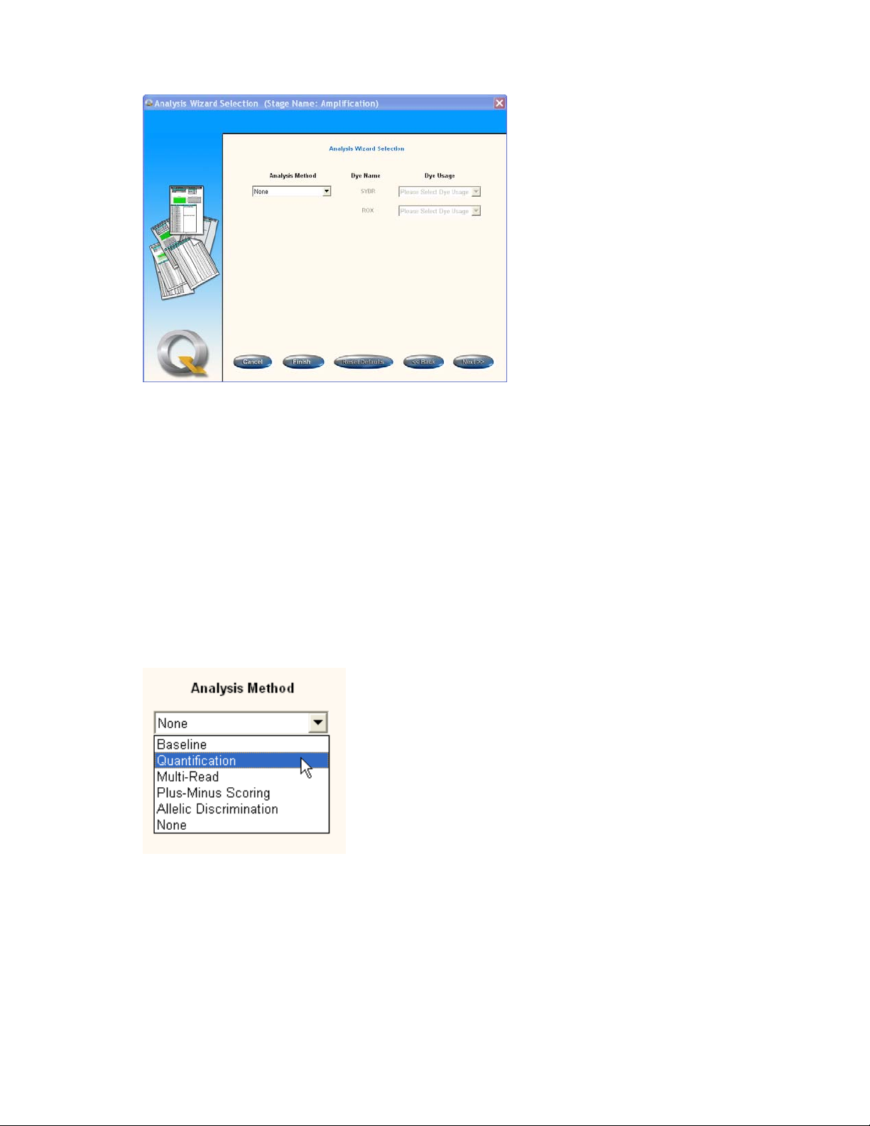
Analysis Method: The drop-down menu allows an analysis method to be selected.
Dye name: The name of the dyes selected in the program setup will be displayed.
Dye Usage: Assign a Dye Usage from the list in the drop-down menu. There will be one dye
usage box for each read present in the selection stage.
Cancel: Aborts the procedure and takes the user back to the Experiment Editor.
Finish: Accepts all the default analysis settings for the analysis method chosen and closes
the Wizard.
Reset defaults: Pressing this button returns all analysis parameter settings to the default.
Back/Next: Allows the user to move between screens in the Analysis Wizard.
The Analysis Method drop-down menu lists analysis types appropriate to the selected stage.
These will be dependent on the number of reads and the number of cycles programmed into the
run (see Choosing an analysis method in section 4.2)
PrimeQ supports the following analysis methods:
No analysis method defined (None)
Baseline correction
Quantification, including:
a. Absolute quantification
b. Relative quantification
c. Relative quantification cycles (Cq)
84

Dissociation curve
Plus/minus scoring
Allelic discrimination
Multi-read
See Chapter 4 for a specific discussion of each analysis method in terms of requirements, setup
and what each approach can reveal about the experimental data.
3.4.5.3 Assigning a dye usage
As there may be more than one dye reading in a single stage, the role of each dye needs to be
assigned. To do this, the Analysis Wizard Selection box has a drop-down menu containing a list of
definitions for each. All definitions are treated as reporters apart from the passive reference dye
(PRD). When the analysis method is undefined or set to ‘none’ then the dye usage selection boxes
are disabled (greyed-out).
It is important to note that if an instrument is not connected and the experiment is not a template
from a previous run then dyes cannot be assigned until an instrument is connected.
Click Next to move through to the Analysis Wizard specific to the analysis method chosen.
3.4.5.4 Analysis wizards
Clicking Next from the Analysis Wizard Selection box branches the Analysis Wizard into the
individual wizards tailored to the particular method of analysis chosen. The parameters displayed
will vary according to the analysis method selected and these are discussed in detail in Chapter 4.
In general the Analysis Wizard will lead the user through the setup procedure as follows:
1. Open the Analysis Wizard:
In the Analysis Selection box in the Experiment Editor, highlight the stage name and click
Edit. The Analysis Wizard Selection screen will appear.
Choose the type of analysis required from the drop-down menu and assign a use for each
dye.
Click Next to open the selected Wizard. The Wizard screens have the following format:
85

2. Passive reference dye (PRD) correction:
Check the box if this correction method is required (only available if a PRD was selected in
the dye usage table). The purpose of the PRD is to normalize the reporter fluorescence and
make well-to-well comparisons more accurate. The readings are normalized by dividing the
fluorescence of the reporter in each well by that of the PRD. This correction method is
applicable to all the analysis types available on PrimeQ (see section 4.4 for more details).
Click Next.
3. Baseline correction method:
This contains a number of options and allows the user to adjust the data for any background
fluorescence. The correction uses the fluorescence readings in the early cycles of the PCR
while fluorescence levels are low, averages out the early noise and subtracts it from
subsequent readings. As with PRD correction, baseline correction can be useful for
correcting the data prior to performing an analysis and so helping to increase the accuracy
of the assay. See Chapter 4 for more details.
Click Next.
4. Set the analysis parameters:
Select suitable parameters for the analysis type chosen e.g. Cq calculation method, which
reads to use for end-point scoring etc. This screen helps the user decide how to choose the
parameters and/or set thresholds accordingly.
5. Report options:
Clicking Next leads through to a window that provides options for choosing which graphs
and tables appear in the report. Separate analysis methods and their report options are
discussed in Chapter 4. The user can choose to select the option to run straight through to
report – see section 3.7.6.3 for more information.
6. Summary:
Clicking Next takes the user through to a page summarizing the settings. Change any
details using the Back function.
Click Finish to complete the setup and return to the Experiment Editor.
Once the Analysis Wizard has completed, the Experiment Editor pane is updated with the selected
analysis method.
86

3.4.6 Saving an experiment to the library
The experiment is now complete with a program file, plate layout and analysis method all defined.
While the program and plate layout can be saved as separate files (shown in 3.4.3.10 and
3.4.4.12), the experiment can also be saved as a consolidated .qexp file at any point during the
setup in the Experiment Editor.
This function can be turned off by simply clicking the padlock icon or by choosing the File option in
the menu bar and clicking on Lock.
On the menu bar in the Experiment Editor, select File and then Save As…
Change the file name as required. If an existing name is selected and the padlock icon is
The .qexp file will automatically be saved to the directory My Documents\Quansoft\Experiments.
Change the destination by browsing the file directories shown in the Save in: drop-down menu.
The library files can be accessed by the quick links on the navigation bar of the Home page
(detailed in section 3.3.3) or by clicking on the Run an Experiment on the Home page, which will
automatically open the Experiment Library folder for browsing.
The destination of all Quansoft files can be changed using the Tools function located on the menu
bar on the Quansoft Home Page. See section 3.4.3.10 for further information.
If the padlock icon in the top-left of the Experiment Editor screen is locked, the current
file in use is designated read only. This provides a useful tool to protect against the
accidental over-writing of files meaning that this file would have to be saved under a
different file name.
IMPORTANT: Certain characters must not be used in the file name otherwise it may
become corrupted and you may not be able to open the Results file. These characters
are: < > & ‘ “
closed, then a warning message will appear asking if the file should be over-written.
3.4.6.1 Editing an experiment
Previous experiments saved in the Experiments folder can be edited for new runs.
Access the Experiment library by clicking on Run an Experiment on the Home Page or
using the Experiment shortcut icon on the navigation bar.
Files can be previewed by clicking on the file name and the contents will be displayed in the lower
pane of the screen.
Double-click on an experiment file to open it in the Experiment Editor. Files are located in
C:\My Documents\ Quansoft\ Experiments.
The experiment opens in the Experiment Editor window.
Each element can be edited in the same way as if creating a blank plate layout, program or setting
up a new analysis.
87

Click Edit in the program or plate layout pane of the Experiment Editor and the appropriate
editor will open.
Change settings in any step/stage, alter readings and so forth or delete the current template
and import another from the library files.
Analysis: Either double-click the name or highlight and press Edit. Make any changes in the
same way as when setting up the analysis. Change the title of experiment if you do not want
to over-write the original file and add any comments if required.
88

3.5 Running an experiment
3.5.1 Starting the run
3.5.1.1 Preparing the system
Turn on the power to PrimeQ using the power switch at the rear of the instrument. An idle
screen will appear on the instrument’s LCD display.
Turn on the PC and log in under a user name.
Double-click the Quansoft icon located on the PC desktop to open the software.
If the instrument has not been used previously, the filter cartridges will need to be installed
(section 1.16).
Prepare and insert the sample plate (as described in section 1.19).
3.5.1.2 Opening the experiment file
Open up the experiment of choice in the Experiment Editor using one of the following options:
Set up a new experiment: Click on Create a New Experiment from the Home Page and
set up a new experiment as detailed in section 3.4.2.
Run an existing experiment: Choose Run an Experiment from the Home Page and
browse the experiment library files (.qexp). Edit any element of an experiment or browse for
separate program (.qprg) or plate layout (.qpla) library files.
Use an experiment from a previous run: An experiment file can be created from a results
file of a previous run by opening a results file in the Results Library (accessible from the
navigator bar of the Quansoft Home page) and selecting Save As Experiment File from the
File menu.
The most important element of the experiment to be considered pre-run is the program as thermal
cycling parameters and read points must be defined to acquire the data. The plate layout and
analysis methods can both be set up or edited post-run.
89

3.5.1.3 Running an experiment
3.5.1.4 Run to report
Unless otherwise informed, the system will wait for an acknowledgment from the user that the run
has ended before proceeding on to analysis and report generation. If Quansoft is required to run
straight through to report generation with no prompt or user intervention then select the Run to
Report option found under Tools on the Experiment Editor menu bar.
Note: running to report is only possible where the analysis type can use the
default parameters or user-defined settings and does not require user
intervention.
3.5.1.5 Starting the run
Click on the Run button in the bottom-right corner of the Experiment Editor window. A
message will appear asking for the action to be confirmed:
Click Yes to confirm.
If the experiment has not already been saved or a previously run experiment is being used and
has been edited, a message will appear asking if the experiment should be saved:
90

Save to the Experiment library folder if required (see section 3.4.6). Note that saving will
over-write the previous version of the experiment.
IMPORTANT: Certain characters must not be used in the file name otherwise it may
become corrupted and you may not be able to open the Results file. These characters
are: < > & ‘ “
A box will now appear asking to save the results in the Results library.
Change the file name of the Results file if required. The file will automatically be saved to
the directory My Documents\Quansoft\Results but the destination can be changed by
browsing the file directory shown in the Save in: drop-down menu. A final message will
appear asking whether to start the run.
Click OK to confirm and the run will initiate
3.5.1.6 Warning messages
The user will be alerted if:
The plate drawer has not been accessed (an indication that a plate has not been loaded).
The lid of the unit is open.
The plate drawer is open.
A prompt will appear requiring the user to confirm that the relevant action has been taken i.e. close
the lid/drawer or load the plate.
91

3.5.1.7 Additional information
If the instrument was not connected when the experiment was created, the correct cartridges will
need to be selected for each read. To select the cartridges, go into the Program Editor from the
Experiment Editor and assign cartridges to each read. Alternately when the run button is pressed
the following error window will appear:
Selecting OK will take the user to the correct window where all of the reads can be assigned a
filter cartridge.
3.5.2 Monitoring the run
3.5.2.1 From the instrument
Progress and current status is reported via the display screen on the front of the instrument.
Cycle cc/mm: Reflects the current cycle number out of the total number for that stage eg.
7/33 is the 7th cycle out of 33. This re-sets after each stage.
xxhyy: Indicates the calculated time remaining for the entire PCR run where xx is hours and
yy is minutes.
Sample: Indicates the current block temperature.
Status: Indicates the current thermal status e.g. ramping or holding.
During a run, pressing the keypad will have the following effect:
Attempts to pause run. The screen will ask for confirmation of the pause command.
Attempts to stop run. The screen will ask for confirmation of the stop command.
Displays the Run Information screen. This displays details of the instrument,
experiment and stage names.
92
ii

3.5.2.2 From the Run Screen
As the PCR is in progress, the Run Screen displays the current status of the program in real time.
Fluorescence data is shown on a per-well basis with the different stages of the run (which have
readings) being displayed as separate tabs. The user can select an individual well to show the
fluorescence data for that well only. The readings are time-stamped and saved in the results data.
If Run to report was chosen from the menu bar, on completion of the run the software will
automatically analyse the data and produce a report based on the user-defined settings.
Instrument information: Displays various details identifying the instrument, experiment
and program. The block temperature, lid temperature and time to completion are also
shown.
Program profile graph: Contains a profile of the PCR program depicting all cycles in the
run. The red line shows the temperature profile while the coloured circles are the dye
reading points (more than one dye is represented by different colours as defined during the
program setup). A vertical line provides the user with a visual representation of how far the
run has progressed. The program name and the stage the program is currently in are both
displayed at the bottom.
Results tabs: Each stage in the program that has been assigned with a read has a tab
labelled with the stage name given during the program setup. The current stage is located
uppermost but the user can click between tabs while the run is in progress to view results
for other stages.
Dye to view: Where multiple readings are being taken, change the reporter being displayed
using the drop-down menu. Only dyes assigned in the setup will be displayed so if only a
single reporter has been assigned, this option will be disabled.
Status lights: Indicate the instrument status
Instrument stopped or faulty
Instrument paused
Instrument run in progress
93
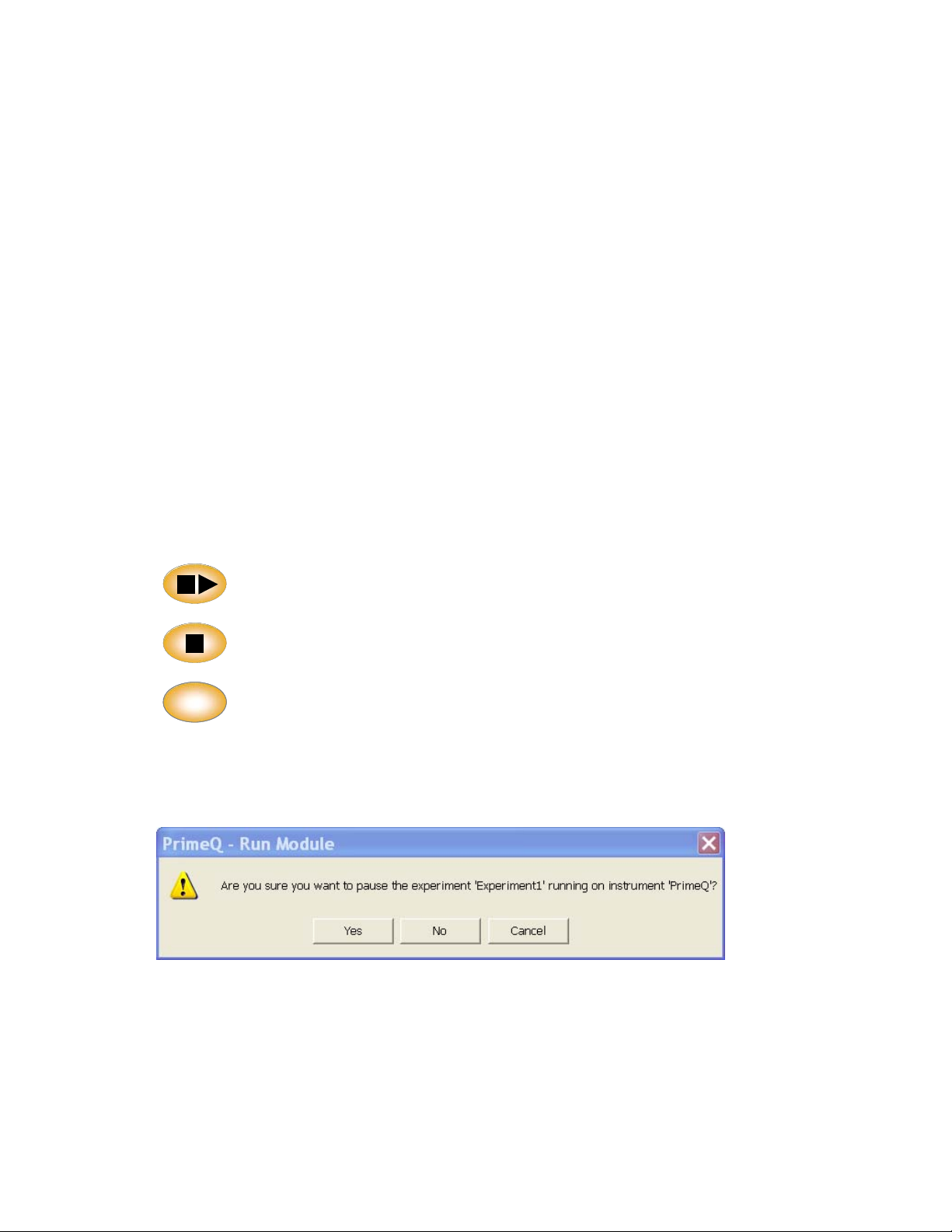
Fluorescence graph: Data for a particular stage will be displayed in the graph. Choose to
display readings for the entire plate or just for selected wells. Change the dye being viewed
using the Dye to View option.
Well view: A fluorescence curve is displayed in each well as the PCR progresses. Highlight
a well(s) with the mouse to display the fluorescence data for that well(s) in the adjacent
graph. To return to viewing all filled wells, click just outside the top left-hand corner of the
plate view. Click again to leave all wells viewed but deselected (highlighted).
Stop/Pause: These commands can be activated from either the PC or the instrument
(provided the instrument buttons were not disabled in the Program setup). If the stop button
is pressed then the user is queried as to whether the run should be stopped. If confirmed,
the instrument is sent an abort command and the software moves into the analysis with
whatever readings have been collected up to that point.
+10 Cycles: Adds 10 cycles to the current stage and is useful if the PCR is progressing
slower than expected.
Skip to Next: Skips the remainder of the current stage and starts the next stage. The
program profile updates accordingly. Note: if skipping to a Ramp Read stage it is
recommended that the skip occurs at the lowest temperature step in the previous cycle.
3.5.3 Stopping or pausing a run
3.5.3.1 From the instrument
The run can be stopped from the instrument LCD control buttons as long as they were not
disabled during program setup.
Press to pause the run. The screen will ask for confirmation of the pause
command.
Press to stop. The screen will ask for confirmation of the stop command.
ii
3.5.3.2 From the Run Screen
The run can be paused or stopped from the Run Screen within Quansoft.
Click the Stop or Pause buttons and confirm the command when prompted.
When a run is paused, the temperature will be held at whatever point the pause was confirmed.
If a run is stopped prematurely, the software does not progress to the analysis screen but alerts
the user as to what has occurred via an information dialogue box.
Information only.
94

3.6 LED intensity settings
Please note the following:
If the fluorescent counts on the raw data plot of the Run Screen or Results Editor are above
100,000 counts using the Medium LED setting, it is recommended that the Low setting be
used for the assay instead.
Similarly, if there are less than 1,000 counts on the Medium setting, use the High LED
setting instead.
95

3.7 Results Editor
3.7.1 Post-run analysis main screen
At the end of a run, if an analysis method was assigned to a stage with a read, the analysed
readings (calculated using either the software defaults or parameters set by the user prior to the
run) will be presented in the Results Editor. If no analysis method was setup, only the raw
fluorescence data will be displayed.
The appearance of the main screen closely resembles that of the Experiment Editor, displaying the
program, plate layout and analysis information in their respective panes and allows the user to
change the plate layout and analysis parameters post-run. The main screen, as shown, is always
the first, left-hand tab.
A. Program pane: Allows the user to view the program settings but not to edit the program (since
the program has completed). As such, the New and Browse functions are greyed-out.
Click View to open the Program within the Program Editor. The program will appear as it did
on setup, the only difference being that the user cannot edit or change any settings.
B. Plate layout pane: Appears as it does in the Experiment Editor and has the same functionality
in terms of editing the layout, browsing for a template from the library files or designing a
layout from new (section 3.4).
C. Analysis Selection: Appears as it does in the Experiment Editor and also has the same
functionality.
Click Edit to enter the Analysis Wizard to view the settings or to change the method of
analysis. The results tab appropriate to the stage will then be updated accordingly. The user
can change any of the parameters and re-analyse the results as many times as desired as
long as the experimental design supports a particular analysis method.
D. Results tabs: The results for each of the program stages assigned a read can be viewed by
clicking on the appropriate tab. The results for each stage are analysed according to the
defined analysis parameters as discussed in Chapter 4.
96

3.7.2 Viewing the results of a run
Click on a results tab on the Results Editor main screen to view the results for a particular stage.
The stage name tab, called here Amplification, brings up the results relevant to that stage
analysed according to the user-defined settings.
A. User and experiment ID: A user name can be entered and comments specific to the
experiment can be added in the Comments box.
B. Results tabs: To the left of the main screen tab are a series of Results Editor tabs. The
uppermost (active) tab displays the Result Editor page as shown. The tabs then list the stages
in the order that they ran. Clicking on the tabs will display the results and graphs relevant to
that particular stage. It is also possible to move between stages from the Results Editor menu
bar.
From the Analysis option, click on Show Stage and then the name of the stage to be
displayed.
Also found on the results tabs is the Log/Audit Trail tab, which provides details of the run
useful for GLP purposes (see section 3.7.5), while the Report tab displays the information
sent to the PrimeQ report (see section 3.7.6).
C. Combine replicates: Clicking this button combines replicate readings to provide an average
for a sample. The button will then change to Show all Samples – click to revert to the
expanded data.
D. Dye to View: Where multiple readings have been taken, the reporter being displayed in the
graphs and results table can be changed using the drop-down menu. This option is disabled if
only one reporter is being used. Note that a PRD is not regarded as a reporter so if one of the
dyes was selected as a PRD in the Analysis Wizard, it will not be listed as available for
viewing.
E. Plate layout: The plate layout is always displayed and shows the colour-coded well types
(standards, unknowns etc.) as defined in the Plate Layout Editor.
Fluorescent readings appear on a per-well basis with a small graph displayed inside each
sample well.
Wells can be selected as in Microsoft
®
Excel (click, ctrl-click, shift-click, drag, select
column/row/all), with only the selected wells appearing on the relevant analysis graphs.
97

Hover the mouse over a particular well for information about the sample type given in a tool-
tip.
Selected wells are persistent between dyes.
Click outside the well plate on the top left hand corner for all filled wells to be viewed;
clicking again leaves all wells viewed but not selected (highlighted).
Right mouse brings up a menu containing Flag wells (or ‘Unflag’ if flagged already). A
flagged well has a cross displayed and is removed from all calculations (appears in the
results table as a strike-through). This is an important tool for selectively eliminating a well
from the calculations.
F. Results table: Contains the calculated results for the run.
The results table can be maximized for improved visibility.
Use the Combine Replicates function to display an average of replicate readings (click
again to revert).
The calculated results will vary according to the method of analysis – see Chapter 4 for
analysis-specific explanation.
G. Graphical display of data: The graphs displayed in the Results Editor will vary according to
the analysis method chosen and the report options selected during setup (further details for
each analysis method can be found in Chapter 4).
The icons found at the top-right of each graph allow the user to:
Maximize a pane – the graph will fill half the screen so aiding visibility.
Minimize a pane – will revert a maximized graph to normal size.
Close a pane – remaining panes will be automatically rearranged.
Brings up the analysis parameters relevant to the graph (see Changing the
analysis parameters in section 3.7.4).
H. Graph icons: Clicking the icons at the top-left allow the user to open any graphs or results
that either have not been shown automatically or that have been actively closed. While
specific icons do appear for specific analysis methods (see Chapter 4), the following examples
are common to all or most analysis methods.
Displays a graph of raw data showing fluorescence plotted against cycle number.
Displays a graph of the background corrected data
Displays a graph showing the block temperature
Displays the results table
Displays a graph of the standard curve (where applicable).
The PrimeQ Report can be printed simply by selecting the Print option within the
Report tab or selecting the print icon.
I. Show All Wells: Clicking this button restores the graphical display of data from all wells if
previously only one or a few wells have been highlighted. This is particularly useful if one of
98

the graphs has been maximized as the user does not have to return to the plate layout display
to re-select the data.
J. Finish/save icons: The results file can be saved at any point during the setup using typical
Windows commands.
However, if the padlock icon in the top-left of the Results Editor screen is locked,
the current file in use is designated read only. This provides a useful tool to protect
against the accidental over-writing of files meaning that if a file of the same name
exists in the destination folder, this file would have to be saved under a different
name. This function can be turned off by clicking on the padlock icon.
The user can also choose to save the experiment as just an experiment file i.e. minus the
results. On the File option on the menu bar, choose Save as Experiment File and the data will
be saved as a .qexp file into the default Experiment Library folder. If the padlock icon is locked
then the file cannot be given the same name as an existing file in the destination folder. Assign
a different name or ‘unlock’ the padlock by clicking the icon in the top-left of the Results Editor.
The user can finish the analysis at any time by selecting the Finish icon. If there have been
any changes made since the results file was last saved, the user will be prompted to save the
file.
3.7.3 Editing a graph
Simple changes to a graph can be made using the right-click mouse function while on the graph
of choice. This will bring up basic options for changing the appearance of a graph.
Change Series Colour: A palette will appear allowing the user to change the colour of the
data points.
Graph scale: Clicking will display the Format Axis settings box. This allows the user to
change the title and scale of the X- or Y-axes. Change as required and then press Done to
finish. This option can also be accessed direct from the menu bar – click on Analysis and
then Graph Scale…
Copy: Copies the graph to the clipboard.
Flag: Removes selected data from the graphical display and subsequent analysis.
Print: Right click and select Print to print any graph.
Change the Graph scale as follows:
X- and Y-axis graph scale: Clicking will display the Format Axis settings box. This allows
the user to change the titles and scales of either the X- or Y-axis.
99

If more sophisticated editing functions are required, access the Graph Properties… option
from the Results Editor menu bar. Select Analysis and then Graph Properties…
The graph editing box is equipped with many features that allow the user to edit different aspects
of the graph including its appearance, the data itself or the print and export options. One of the
most important features is the Export tab which enables the user to export the graphs in different
file formats.
3.7.4 Changing the analysis parameters
A flexible approach to data analysis is provided with the option to re-analyse the results of a run
using different analysis parameters or with a different analysis method entirely (as long as the
experiment design supports the analysis method).
3.7.4.1 Edit analysis parameters
The settings for an analysis method can be viewed and changed from within the Results Editor by
clicking the PAR button next to the graph.
100
 Loading...