
AN3984
Application note
IIR filter design equations for Sound Terminal® devices
Introduction
The purpose of this document is to provide a tool to calculate the IIR filter coefficients to
program the Sound Terminal
For each filter the procedure and the formulas to calculate the coefficient will be described;
the Matlab code is given in Appendix A: Matlab code (functions) on page 24.
A generalized set of equations can be formulated for the design of first-order low-pass and
high-pass filters and of second-order filters.
A specialized set of equations is devised for designing parametric biquad EQ filters. As with
any other filter design procedure, the desired characteristics of the filter are to be made
available.
The parameters governing the characteristics of each filter are:
■ fc: filter cutoff frequency which is the -3dB corner frequency or the midpoint frequency in
a peak or notch filter
■ fs: sampling frequency
■ Q: quality factor (not applicable for low and high-shelf filters)
■ Slope: applicable only for low and high-shelf filters
■ Gain: the boost or the attenuation at f = fc
These parameters can be used to determine the coefficients of the digital filter transfer
function.
®
devices from STMicroelectronics.
September 2011 Doc ID 022240 Rev 1 1/46
www.st.com

Contents AN3984
Contents
1 Overview . . . . . . . . . . . . . . . . . . . . . . . . . . . . . . . . . . . . . . . . . . . . . . . . . . 5
2 Filter stability . . . . . . . . . . . . . . . . . . . . . . . . . . . . . . . . . . . . . . . . . . . . . . . 6
2.1 Definition . . . . . . . . . . . . . . . . . . . . . . . . . . . . . . . . . . . . . . . . . . . . . . . . . . 6
2.2 First-order filter . . . . . . . . . . . . . . . . . . . . . . . . . . . . . . . . . . . . . . . . . . . . . . 6
2.3 Second-order filter . . . . . . . . . . . . . . . . . . . . . . . . . . . . . . . . . . . . . . . . . . . 6
3 First-order filter design (LPF and HPF) . . . . . . . . . . . . . . . . . . . . . . . . . . 7
4 Second-order filter design . . . . . . . . . . . . . . . . . . . . . . . . . . . . . . . . . . . . 8
4.1 Low-pass and high-pass filters . . . . . . . . . . . . . . . . . . . . . . . . . . . . . . . . . . 8
4.1.1 Low-pass filter . . . . . . . . . . . . . . . . . . . . . . . . . . . . . . . . . . . . . . . . . . . . . 8
4.1.2 High-pass filter . . . . . . . . . . . . . . . . . . . . . . . . . . . . . . . . . . . . . . . . . . . . . 9
4.2 Peak filters . . . . . . . . . . . . . . . . . . . . . . . . . . . . . . . . . . . . . . . . . . . . . . . . 10
4.2.1 Peak filter - negative gain (cut) . . . . . . . . . . . . . . . . . . . . . . . . . . . . . . . 10
4.2.2 Peak filter - positive gain (boost) . . . . . . . . . . . . . . . . . . . . . . . . . . . . . . 11
4.3 Shelf filters . . . . . . . . . . . . . . . . . . . . . . . . . . . . . . . . . . . . . . . . . . . . . . . . 12
4.3.1 Low-shelf filter . . . . . . . . . . . . . . . . . . . . . . . . . . . . . . . . . . . . . . . . . . . . 12
4.3.2 High-shelf filter . . . . . . . . . . . . . . . . . . . . . . . . . . . . . . . . . . . . . . . . . . . . 13
4.4 Notch filter . . . . . . . . . . . . . . . . . . . . . . . . . . . . . . . . . . . . . . . . . . . . . . . . 13
4.5 All-pass filter . . . . . . . . . . . . . . . . . . . . . . . . . . . . . . . . . . . . . . . . . . . . . . . 14
4.6 Band-pass filter . . . . . . . . . . . . . . . . . . . . . . . . . . . . . . . . . . . . . . . . . . . . 14
5 Examples . . . . . . . . . . . . . . . . . . . . . . . . . . . . . . . . . . . . . . . . . . . . . . . . . 15
5.1 1st-order low-pass filter . . . . . . . . . . . . . . . . . . . . . . . . . . . . . . . . . . . . . . . 15
5.2 1
5.3 2
5.4 2
5.5 Low-shelf filter . . . . . . . . . . . . . . . . . . . . . . . . . . . . . . . . . . . . . . . . . . . . . 19
5.6 High-shelf filter . . . . . . . . . . . . . . . . . . . . . . . . . . . . . . . . . . . . . . . . . . . . . 20
st
-order high-pass filter . . . . . . . . . . . . . . . . . . . . . . . . . . . . . . . . . . . . . . 16
nd
-order low-pass filter . . . . . . . . . . . . . . . . . . . . . . . . . . . . . . . . . . . . . . 17
nd
-order high-pass filter . . . . . . . . . . . . . . . . . . . . . . . . . . . . . . . . . . . . . 18
5.7 Notch filter . . . . . . . . . . . . . . . . . . . . . . . . . . . . . . . . . . . . . . . . . . . . . . . . 21
5.8 All-pass filter . . . . . . . . . . . . . . . . . . . . . . . . . . . . . . . . . . . . . . . . . . . . . . . 22
5.9 Band-pass filter . . . . . . . . . . . . . . . . . . . . . . . . . . . . . . . . . . . . . . . . . . . . 23
2/46 Doc ID 022240 Rev 1

AN3984 Contents
Appendix A Matlab code (functions). . . . . . . . . . . . . . . . . . . . . . . . . . . . . . . . . . . 24
A.1 Code structure. . . . . . . . . . . . . . . . . . . . . . . . . . . . . . . . . . . . . . . . . . . . . . 24
A.2 Peak filter (PeakFilterAPW.m) . . . . . . . . . . . . . . . . . . . . . . . . . . . . . . . . . . 25
A.3 Low-pass and high-pass filter (LHPassFilterAPW.m) . . . . . . . . . . . . . . . . 27
A.4 Low and high-shelf filter (ShelfFilterAPW.m). . . . . . . . . . . . . . . . . . . . . . . 30
A.5 Notch filter (NotchFilterAPW.m) . . . . . . . . . . . . . . . . . . . . . . . . . . . . . . . . 33
A.6 All-pass filter (AllPassFilterAPW.m). . . . . . . . . . . . . . . . . . . . . . . . . . . . . . 35
A.7 Band-pass filter (BandPassFilterAPW.m) . . . . . . . . . . . . . . . . . . . . . . . . . 37
A.8 Float to hex conversion (myFloat2Hex.m) . . . . . . . . . . . . . . . . . . . . . . . . . 39
A.9 Max coefficient limit value calculator (LimitVal.m) . . . . . . . . . . . . . . . . . . . 40
A.10 Display coefficient and error messages (Display_Coeff.m). . . . . . . . . . . . 41
Appendix B Abbreviations and acronyms . . . . . . . . . . . . . . . . . . . . . . . . . . . . . . 44
6 Revision history . . . . . . . . . . . . . . . . . . . . . . . . . . . . . . . . . . . . . . . . . . . 45
Doc ID 022240 Rev 1 3/46

List of figures AN3984
List of figures
Figure 1. 1st-order low-pass filter - magnitude response . . . . . . . . . . . . . . . . . . . . . . . . . . . . . . . . . . 15
Figure 2. 1
Figure 3. 2
Figure 4. 2
Figure 5. Low-shelf filter - magnitude response. . . . . . . . . . . . . . . . . . . . . . . . . . . . . . . . . . . . . . . . . 19
Figure 6. High-shelf filter - magnitude response . . . . . . . . . . . . . . . . . . . . . . . . . . . . . . . . . . . . . . . . 20
Figure 7. Notch filter - magnitude response. . . . . . . . . . . . . . . . . . . . . . . . . . . . . . . . . . . . . . . . . . . . 21
Figure 8. All-pass filter - phase response . . . . . . . . . . . . . . . . . . . . . . . . . . . . . . . . . . . . . . . . . . . . . 22
Figure 9. Band-pass filter - magnitude response . . . . . . . . . . . . . . . . . . . . . . . . . . . . . . . . . . . . . . . . 23
Figure 10. Code structure . . . . . . . . . . . . . . . . . . . . . . . . . . . . . . . . . . . . . . . . . . . . . . . . . . . . . . . . . . 24
st
-order high-pass filter - magnitude response . . . . . . . . . . . . . . . . . . . . . . . . . . . . . . . . . 16
nd
-order low-pass filter - magnitude response . . . . . . . . . . . . . . . . . . . . . . . . . . . . . . . . . 17
nd
-order high-pass filter - magnitude response. . . . . . . . . . . . . . . . . . . . . . . . . . . . . . . . . 18
4/46 Doc ID 022240 Rev 1
AN3984 Overview
1 Overview
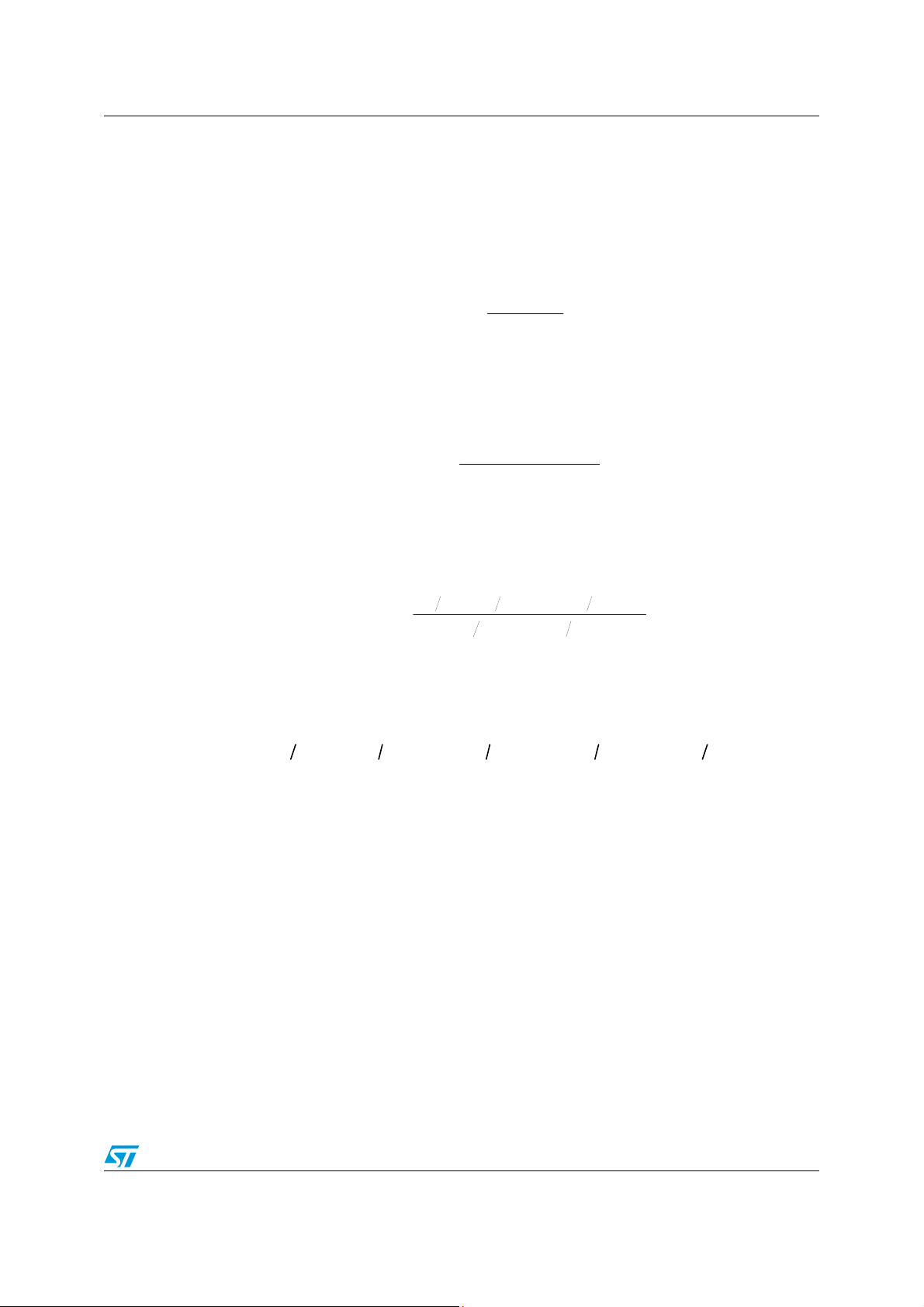
The transfer function for a first-order filter in the digital z-domain is:
Equation 1
1
−
zbb
⋅+
)z(H
=
For a second-order filter (a biquad) the transfer function is:
Equation 2
)(
=
zH
This equation can be modified normalizing the a0 coefficient; the new equation is:
Equation 3
()() ()
)(
=
zH
() ()
1
10
1
−
zaa
⋅+
10
1
10
1
10
0100
1
01
2
−−
⋅+⋅+
zbzbb
2
2
−−
⋅+⋅+
zazaa
2
1
02
2
−−
⋅+⋅+
zabzabab
02
2
−−
⋅+⋅+
zaazaa
The most straightforward implementation form using Equation 3 is:
Equation 4
() () () () ()
]2n[yaa]1n[yaa]2n[xab]1n[xab]n[xab]n[y
−⋅−−⋅−−⋅+−⋅+⋅=
0201020100
Doc ID 022240 Rev 1 5/46
Filter stability AN3984
2 Filter stability
2.1 Definition
A filter is said to be stable in the z-domain if the roots (or poles) of the filter lie inside the unit
circle.
This definition of stability can be translated in terms of the filter coefficients.
2.2 First-order filter
For a first-order filter, the stability condition that needs to be satisfied is that the pole of the
filter lies within the unit circle.
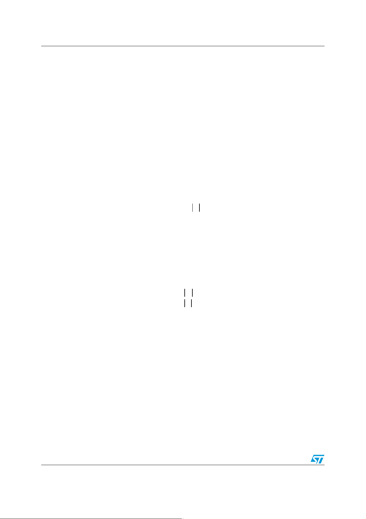
In terms of the coefficients, the condition can be given as:
Equation 5
11<a
2.3 Second-order filter
For a 2nd-order filter, two conditions must be satisfied to ensure filter stability and translated
in terms of the filter coefficients they are:
Equation 6
a+<<
1
2
)1(
aa
21
6/46 Doc ID 022240 Rev 1
AN3984 First-order filter design (LPF and HPF)
3 First-order filter design (LPF and HPF)
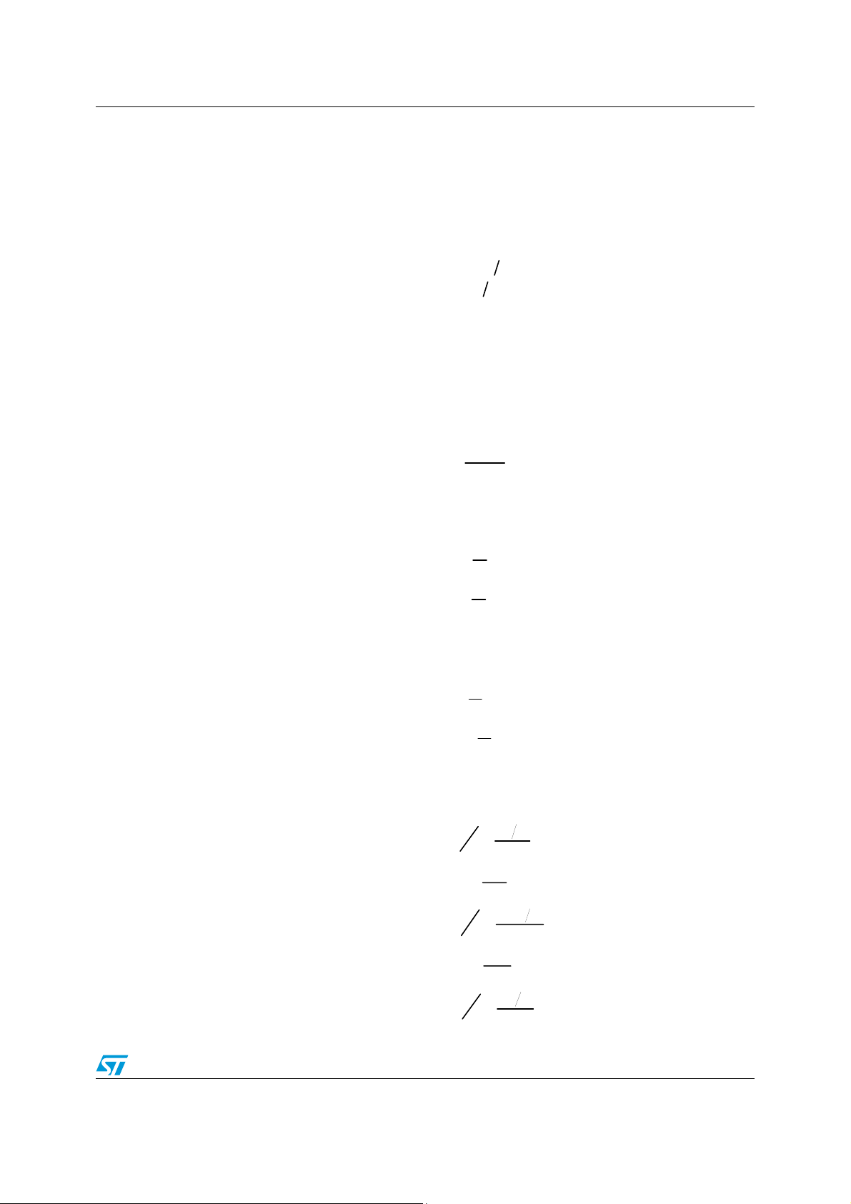
The preliminary step to obtain the coefficients for the first-order low-pass filter or high-pass
filter is to define three constants obtained from the filter parameters:
Equation 7
ff
⋅⋅=
2
πω
K
α
()
=
ω
K
+=
1
scc
2tan
c
In a first-order filter both the coefficients a
and b2 are null.
2
The denominator coefficients are identical for both an LPF and an HPF designed for the
same cutoff frequency and they are computed as follows:
Equation 8
a
=11
0
()
K
a
1
−
−=
α
The numerator for an LPF can be calculated as follows:
Equation 9
K
b==
0
α
K
b
1
α
The numerator for an HPF can be calculated as follows:
Equation 10
1
b
0
α
1
−==b
1
α
The coefficient used in APWorkbench can be calculated by applying these formulas:
Equation 11
b
()
b
1
t Coefficien
2
t bCoefficien
=
2
a
1
t Coefficien
2
=
t aCoefficien
2
b
0
t Coefficien
2
Doc ID 022240 Rev 1 7/46
2
1
=
a
0
()
b
2
a
0
()
2
a
−
1
=
a
0
−
a
2
a
0
()
2
b
0
=
a
0
Second-order filter design AN3984
4 Second-order filter design
4.1 Low-pass and high-pass filters
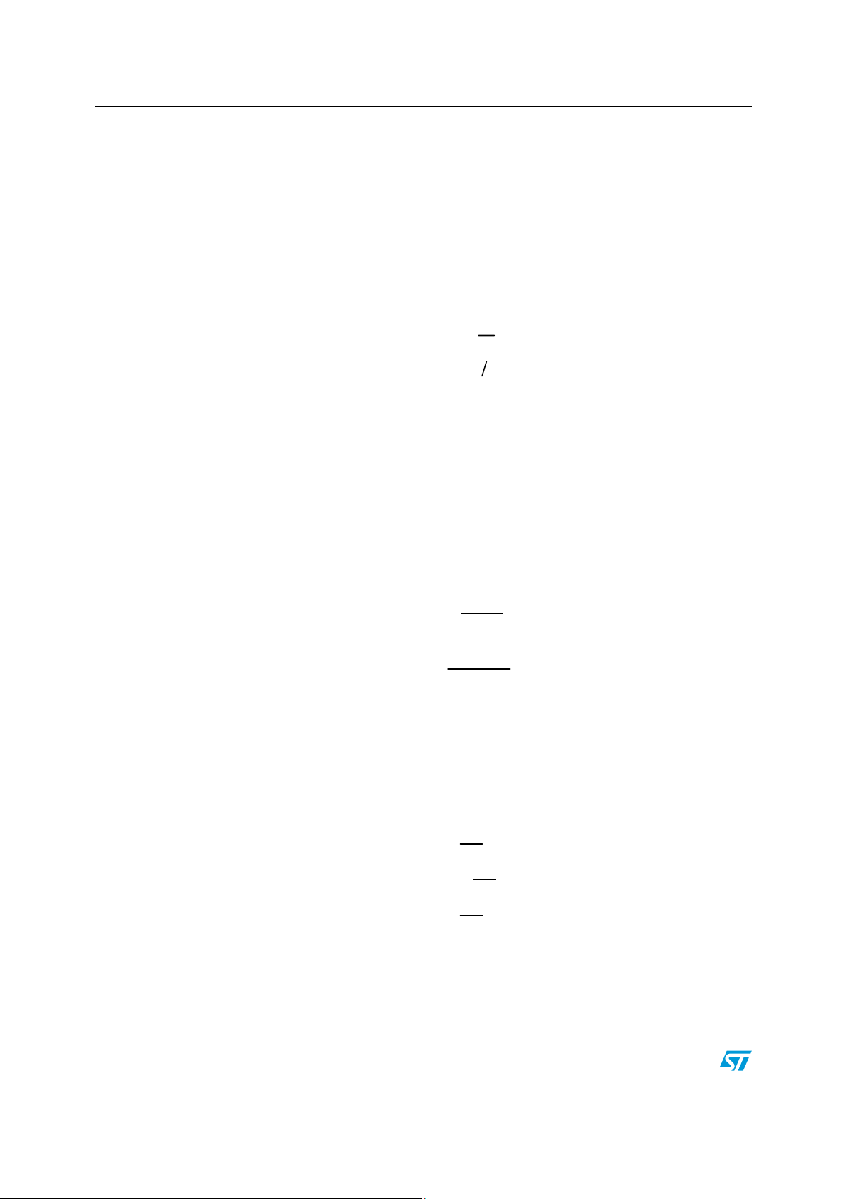
The preliminary step to obtain the coefficients for a second-order filter is the calculation of
these coefficients obtained from the filter parameters:
Equation 12
f
c
πϑ
⋅⋅=
2
c
K
=
=
α
DE
The denominator coefficients are the same for both an LPF and an HPF if designed for the
same cutoff frequency. They are computed as follows:
f
s
ω
()
2tan
c
2
KW
K
+=
1
K
W
++=
1
Q
Equation 13
4.1.1 Low-pass filter
The numerator coefficient for a second-order LPF can be calculated as follows:
Equation 14
=
1
a
0
−
1
W
()
⋅=
2
a
1
a
2
DE
K
1
=
=
b
0
b
1
=
b
2
DE
2
DE
W
W
Q
DE
⋅=
W
DE
W
+−
8/46 Doc ID 022240 Rev 1
AN3984 Second-order filter design
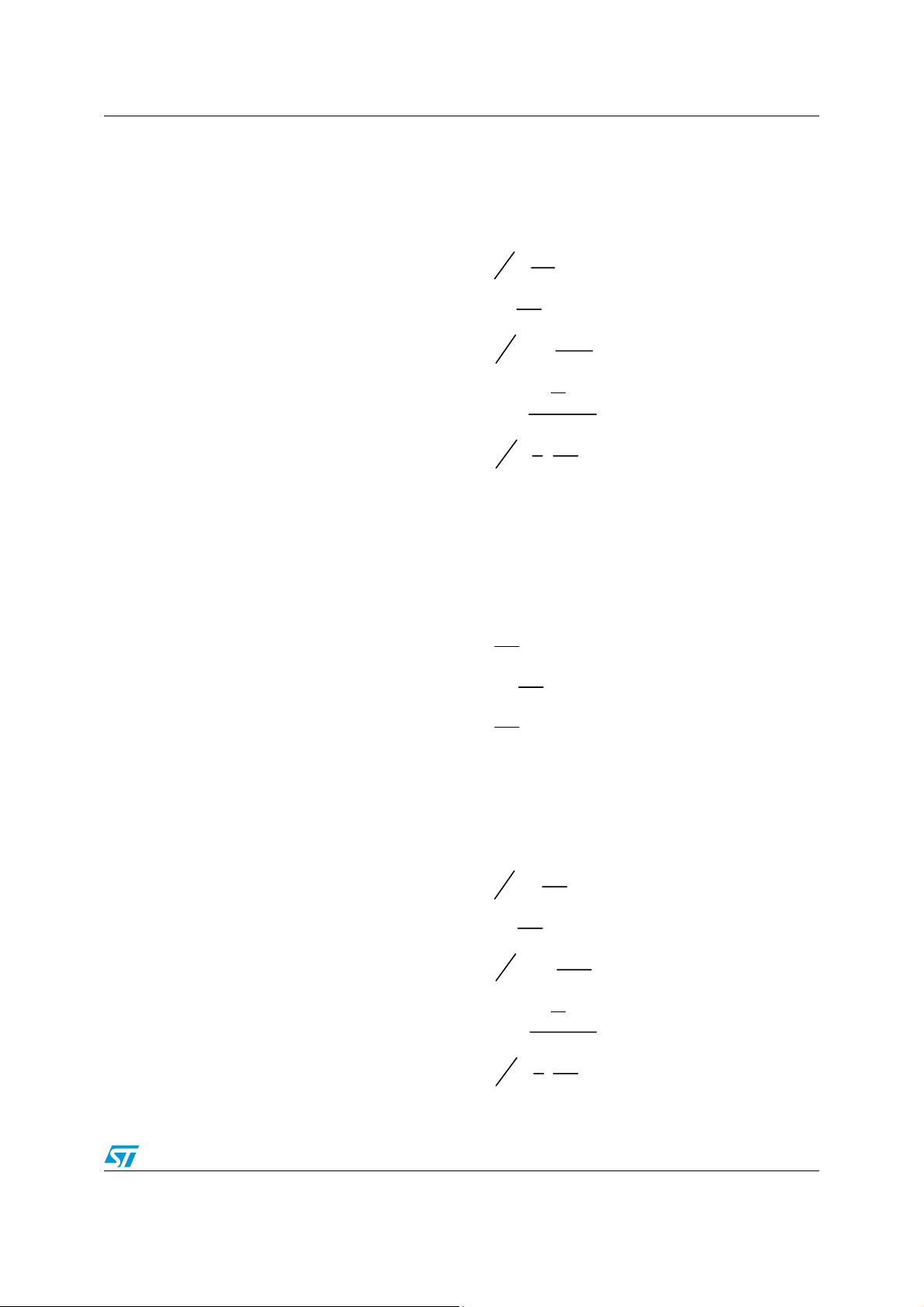
For a second-order LPF, the coefficients given in APWorkbench can be calculated as
follows:
Equation 15
W
b
1
t Coeffi cien
=
2
DE
W
t bCoeffi cien
=
2
DE
W
1
a
1
t Coeffi cien
2
t aCoeffi cien
−=
2
b
0
t Coeffi cien
2
−
1
⋅−=
DE
K
1
W
+−
Q
DE
W
1
⋅=
DE
2
4.1.2 High-pass filter
The numerator coefficient for a second-order HPF can be calculated as follows:
Equation 16
1
b
=
0
DE
W
2
⋅−=
b
1
b
DE
1
=
2
DE
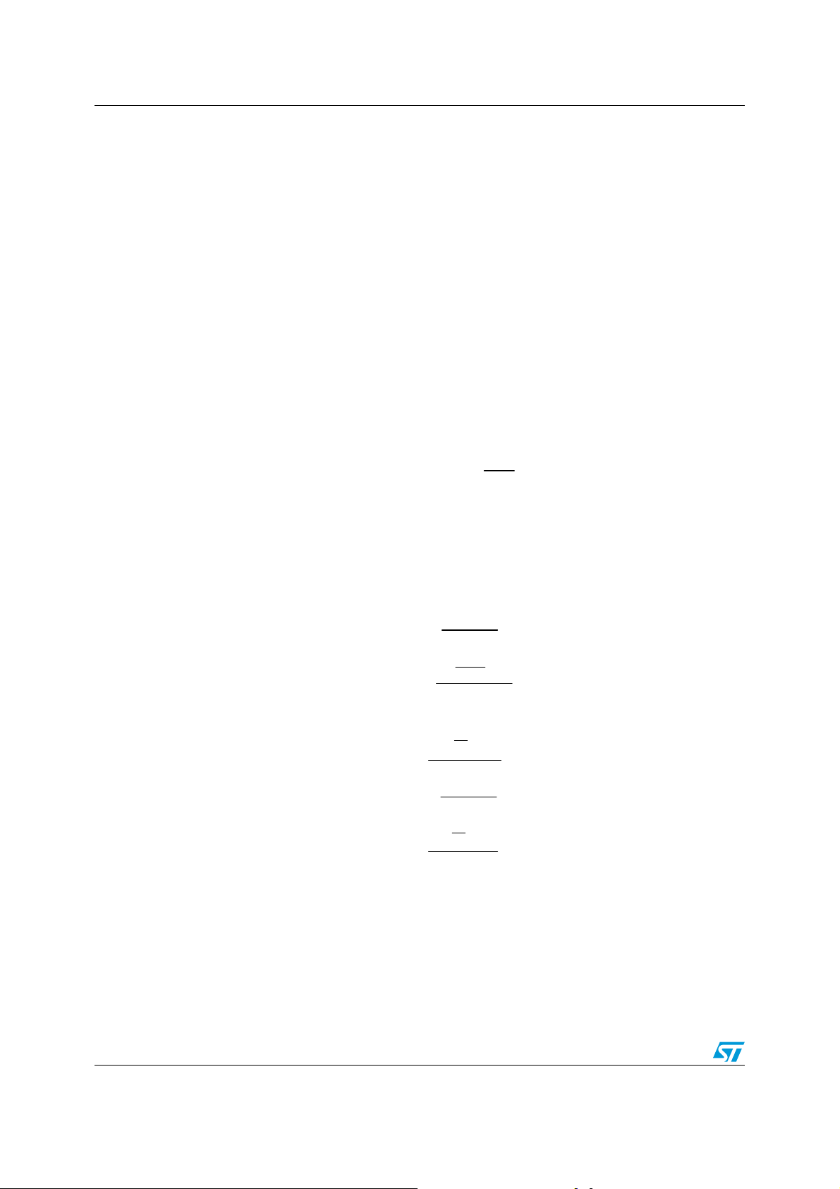
For a second-order HPF, the coefficients given in APWorkbench can be calculated as
follows:
Equation 17
b
1
t Coefficien
2
t bCoefficien
2
a
1
t Coefficien
t aCoefficien
2
b
0
t Coefficien
1
−=
DE
1
=
DE
−
W
1
⋅−=
1
2
2
DE
K
+−
1
−=
W
Q
DE
1
1
⋅=
DE
2
Doc ID 022240 Rev 1 9/46
Second-order filter design AN3984
4.2 Peak filters
The first step is the calculation of the constant gain obtained from the gain filter parameter
(GdB is expressed in dB).
Equation 18
The filter coefficients are different if the gain is positive or negative.
4.2.1 Peak filter - negative gain (cut)
The cut value is calculated with the following equation:
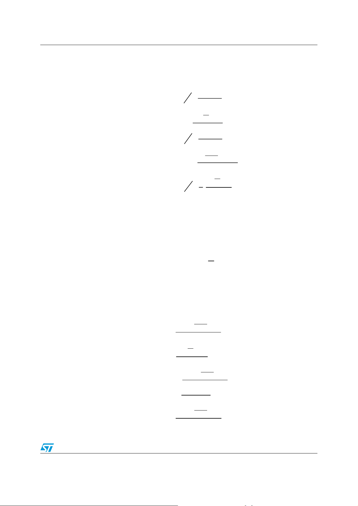
Equation 19
The filter coefficient can be calculated as follows:
Equation 20
a
0
a
1
a
2
b
0
b
1
b
2
GainGain
=
1
()
W
⋅=
4
CutValue
⎛
1
⎜
⎜
=
⎜
CutValue
⎜
⎝
⎛
⎜
1
⎜
⎝
=
CutValue
()
W
⋅=
2
CutValue
K
Q
=
CutValue
dB
Q
⎛
KCutValue +⎟
⎜
⋅+= 1
Gain
⎝
−
1
Q
+−
W
Gain
⎞
K
⎟
++
W
⎟
Q
⎠
−
1
+−
W
)1(
)115129 254.0exp( ⋅=
⎞
W
⎠
⎞
⎟
⎟
⎟
⎟
⎠
10/46 Doc ID 022240 Rev 1
AN3984 Second-order filter design
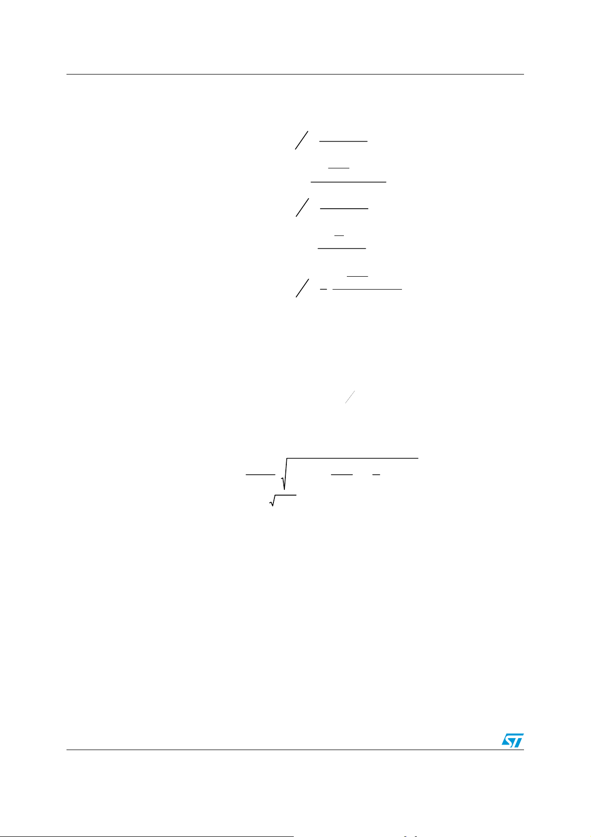
The coefficients in the APWorkbench are consequently calculated as follows:
Equation 21
−
W
b
1
=
t Coefficien
2
=
t bCo effic ien
2
a
1
=
t Coefficien
2
−=
t aCo effic ien
2
b
0
t Coefficien
2
1
CutVa lue
K
+−
W
Q
CutValue
−
1
W
CutVa lue
Q
1
Gain
CutValue
1
1
⋅=
2
CutValue
)1(
WK
+⋅−
K
W
++
Q
4.2.2 Peak filter - positive gain (boost)
The boost value is calculated with the following equation:
Equation 22
K
BoostValue ++= 1
W
Q
The filter coefficient can be calculated as follows:
Equation 23
=
a
1
0
Gain
+⋅+
=
a
1
=
a
2
b
0
b
1
=
b
2
K
BoostValue
⎛
K
⎜
1
⎜
Q
⎝
BoostValue
K
⋅=
2
BoostValue
W
⋅=
2
BoostValue
K
BoostValue
Q
+−
W
Gain
−
1
Gain
Q
W
)1(
⎞
⎟
⎟
⎠
+⋅+
W
Q
+⋅−
W
)1(
)1(
Doc ID 022240 Rev 1 11/46
Second-order filter design AN3984
The coefficients in the APWorkbench are consequently calculated as follows:
Equation 24
W
−
b
1
t Coefficien
=
2
=
t bCoefficien
2
a
1
t Coefficien
=
2
−=
t aCoefficien
2
BoostValue
b
0
t Coefficien
2
1
Boo stValue
Gain
Q
BoostValue
−
1
W
BoostValue
K
W
+−
1
Q
Gain
1
1
2
⋅=
BoostValue
Q
WK
+⋅−
)1(
+⋅+
WK
4.3 Shelf filters
The coefficient gain is defined in Equation 25.
Equation 25
The coefficients α and β are calculated as follows:
Equation 26
4.3.1 Low-shelf filter
The coefficients for an LSF can be calculated as follows:
Equation 27
10
Gain =
sin
α
2
αβ
2
()()
0
1
()()
2
0
1
2
⎛
()
ϑ
⎛
c
⎜
⎜
Gain
⎜
⎜
⎝
⎝
Gain
⋅⋅=
GainGaina
()()
Ga inGaina
GainGaina
()()()
()()()
()()()
Ga in
dB
(
⎛
+⋅=
⎜
⎝
)
40
11
⎞
⎛
⎞
⎟
−⋅
⎜
⎟
⎟
SGain
⎝
⎠
⎠
βϑ
+⋅−++=
cos11
c
ϑ
⋅++−⋅−=
cos112
c
βϑ
−⋅−++=
cos11
c
GainGainGai nb
Gai nGainGainb
GainGainGai nb
cos11
⋅+−−⋅⋅=
cos112
co s11
⎞
⎞
⎟
21
+
⎟
⎟
⎠
⎠
βϑ
+⋅−−+⋅=
c
ϑ
c
βϑ
−⋅−−+⋅=
c
The coefficient to load in APWorkbench can be calculated by applying the calculation
already shown in Equation 11.
12/46 Doc ID 022240 Rev 1

AN3984 Second-order filter design
4.3.2 High-shelf filter
The coefficients for an HSF can be calculated as follows:
Equation 28
()()
0
()()
1
()()
2
0
1
2
GainGaina
Gai nGaina
GainGaina
()()()
()()()
()()()
cos11
cos11
GainGainGai nb
Gai nGainGainb
GainGainGai nb
βϑ
+⋅−−+=
c
ϑ
⋅+−−⋅=
cos112
c
βϑ
−⋅−−+=
c
βϑ
+⋅−++⋅=
co s11
c
ϑ
⋅+−−⋅⋅−=
cos112
c
βϑ
−⋅−++⋅=
cos11
c
The coefficient to load in APWorkbench to program a HSF can be computed by applying the
formulas shown in Equation 11.
4.4 Notch filter
The first step is to define the constant α
Equation 29
(a)
:
()
ϑ
sin
α
Qc⋅=2
The coefficients for a notch filter can be calculated as follows:
Equation 30
α
1
+=
a
0
ϑ
cos2
a
a
b
b
b
⋅−=
1
1
2
1
=
0
1
1
=
2
c
α
−=
ϑ
cos2
⋅−=
The coefficients to load in APWorkbench can be calculated using Equation 11.
a. ϑc is defined in Equation 12
Doc ID 022240 Rev 1 13/46

Second-order filter design AN3984
4.5 All-pass filter
Equation 29 allows calculating the constant α.
The coefficients for an APF can be calculated as follows:
Equation 31
1
α
+=
a
0
cos2
ϑ
⋅−=
a
1
1
a
2
1
−=
b
0
1
+=
b
2
c
α
−=
α
cos2
ϑ
=⋅−=
ab
c
11
α
The coefficients to load in APWorkbench can be calculated using Equation 11.
4.6 Band-pass filter
Equation 29 allows calculating the constant α while Equation 32 is used to calculate the
normalized gain.
Equation 32
⎛
⎞
Ga in
dB
⎜
⎟
⎝
(b)
⎠
:
NormGain
=2010
The coefficients for a BPF can be calculated as follows
Equation 33
a
+=
α
1
0
a
a
b
⋅−=
ϑ
1
2
0
1
cos2
c
−=
α
1
NormGainb
⋅=
α
=
0
NormGainbb
⋅−=−=
α
02
The coefficients to load in APWorkbench can be calculated using Equation 11.
b. α is defined in Equation 29, ϑc is defined in Equation 12.
14/46 Doc ID 022240 Rev 1

AN3984 Examples
5 Examples
5.1 1st-order low-pass filter
Input data:
● Cutoff freq: 1 kHz
● Coefficient range: 4
● Processing frequency: 96 kHz
Output data:
Filter coefficients
'Coeff 1: b1/2' 'Coeff 2: b2' 'Coeff 3: -a1/2' 'Coeff 4: -a2' 'Coeff 5: b0/2'
'0081d6' '000000' '0efc52' '000000' '0081d6'
Figure 1. 1st-order low-pass filter - magnitude response
Magnitude Respons e (dB)
0
-5
-10
Magnitude (dB)
-15
-20
-1
10
Frequency ( kHz)
0
10
1
10
Doc ID 022240 Rev 1 15/46

Examples AN3984
5.2 1st-order high-pass filter
Input data:
● Cutoff freq: 1 kHz
● Coefficient range: 4
● Processing frequency: 96 kHz
Output data:
Filter coefficients
'Coeff 1: b1/2' 'Coeff 2: b2' 'Coeff 3: -a1/2' 'Coeff 4: -a2' 'Coeff 5: b0/2'
'f081d6' '000000' '0efc52' '000000' '0f7e29'
Figure 2. 1st-order high-pass filter - magnitude response
Magnitude Respons e (dB)
0
-5
-10
Magnitude (dB)
-15
-20
-1
10
Frequency ( kHz)
0
10
1
10
16/46 Doc ID 022240 Rev 1

AN3984 Examples
5.3 2nd-order low-pass filter
Input data:
● Cutoff freq: 1 kHz
● Coefficient range: 4
● Quality factor (Q): 2
● Processing frequency: 96 kHz
Output data:
Filter coefficients
'Coeff 1: b1/2' 'Coeff 2: b2' 'Coeff 3: -a1/2' 'Coeff 4: -a2' 'Coeff 5: b0/2'
'0008a0' '0008a0' '1f6af3' 'e10794' '000450'
Figure 3. 2nd-order low-pass filter - magnitude response
15
10
5
0
-5
-10
-15
Magnitude (dB)
-20
-25
-30
-35
-40
-1
10
Magnitude Respons e (dB)
0
Frequency ( kHz)
10
1
10
Doc ID 022240 Rev 1 17/46

Examples AN3984
5.4 2nd-order high-pass filter
Input data:
● Cutoff freq: 1 kHz
● Coefficient range: 4
● Quality factor (Q): 2
● Processing frequency: 96 kHz
Output data:
Filter coefficients
'Coeff 1: b1/2' 'Coeff 2: b2' 'Coeff 3: -a1/2' 'Coeff 4: -a2' 'Coeff 5: b0/2'
'e08c6b' '1f7394' '1f6af3' 'e10794' '0fb9ca'
Figure 4. 2nd-order high-pass filter - magnitude response
20
10
0
-10
Magnitude (dB)
-20
-30
-40
-1
10
Magnitude Respons e (dB)
0
Frequency ( kHz)
10
1
10
18/46 Doc ID 022240 Rev 1

AN3984 Examples
5.5 Low-shelf filter
Input data:
● Cutoff freq: 1 kHz
● Gain: -10 dB
● Coefficient range: 4
● Slope: 2
● Processing frequency: 96 kHz
Output data:
Filter coefficients
'Coeff 1: b1/2' 'Coeff 2: b2' 'Coeff 3: -a1/2' 'Coeff 4: -a2' 'Coeff 5: b0/2'
'e0f9f2' '1e8e49' '1efbb2' 'e1cc06' '0fc87d'
Figure 5. Low-shelf filter - magnitude response
5
0
-5
Magnitude (dB)
-10
-15
-20
-1
10
Magnitude Respons e (dB)
0
Frequency ( kHz)
10
1
10
Doc ID 022240 Rev 1 19/46

Examples AN3984
5.6 High-shelf filter
Input data:
● Cutoff freq: 1 kHz
● Gain: -10 dB
● Coefficient range: 4
● Slope: 2
● Processing frequency: 96 kHz
Output data:
Filter coefficients
'Coeff 1: b1/2' 'Coeff 2: b2' 'Coeff 3: -a1/2' 'Coeff 4: -a2' 'Coeff 5: b0/2'
'f61151' '09aea8' '1f732a' 'e1063e' '052110'
Figure 6. High-shelf filter - magnitude response
5
0
-5
Magnitude (dB)
-10
-15
-1
10
Magnitude Respons e (dB)
0
Frequency ( kHz)
10
1
10
20/46 Doc ID 022240 Rev 1

AN3984 Examples
5.7 Notch filter
Input data:
● Cutoff freq: 1 kHz
● Quality factor: 0.5
● Coefficient range: 4
● Processing frequency: 96 kHz
Output data:
Filter coefficients
'Coeff 1: b1/2' 'Coeff 2: b2' 'Coeff 3: -a1/2' 'Coeff 4: -a2' 'Coeff 5: b0/2'
'e2075a' '1e091b' '1df8a5' 'e3edc8' '0f048d'
Figure 7. Notch filter - magnitude response
Magnitude Respons e (dB)
0
-10
-20
-30
Magnitude (dB)
-40
-50
-60
-1
10
Frequency ( kHz)
0
10
1
10
Doc ID 022240 Rev 1 21/46

Examples AN3984
5.8 All-pass filter
Input data:
● Cutoff freq: 1 kHz
● Quality factor: 5
● Coefficient range: 4
● Processing frequency: 96 kHz
Output data:
Filter coefficients
'Coeff 1: b1/2' 'Coeff 2: b2' 'Coeff 3: -a1/2' 'Coeff 4: -a2' 'Coeff 5: b0/2'
'e046a7' '200000' '1fb958' 'e06a75' '0fcac5'
Figure 8. All-pass filter - phase response
Phase Res ponse
0
-1
-2
-3
Phase (radians )
-4
-5
-6
-1
10
Frequency ( kHz)
0
10
1
10
22/46 Doc ID 022240 Rev 1

AN3984 Examples
5.9 Band-pass filter
Input data:
● Cutoff freq: 1 kHz
● Gain: +6 dB
● Quality factor: 3
● Coefficient range: 4
● Processing frequency: 96 kHz
Output data:
Filter coefficients
'Coeff 1: b1/2' 'Coeff 2: b2' 'Coeff 3: -a1/2' 'Coeff 4: -a2' 'Coeff 5: b0/2'
'000000' 'ff4fc0' '1f9650' 'e0b0ab' '00581f'
Figure 9. Band-pass filter - magnitude response
10
5
0
-5
-10
-15
Magnitude (dB)
-20
-25
-30
-35
-40
-1
10
Magnitude Respons e (dB)
0
Frequency ( kHz)
10
1
10
Doc ID 022240 Rev 1 23/46

Matlab code (functions) AN3984
Appendix A Matlab code (functions)
A.1 Code structure
Figure 10. Code structure
Start
Filter data
(cutoff freq, gain,…)
Coefficient
calculation
Coefficient limit
calculation
Float to Hex
Conversion
Coefficients and Filter
stability check
Display coefficient
End
24/46 Doc ID 022240 Rev 1

AN3984 Matlab code (functions)
A.2 Peak filter (PeakFilterAPW.m)
%-------------------------------------------------------------------------%
% function [Coeff_Hex, CoeffAPW, LimitVal] = PeakFilterAPW(Fc, Gain, Q,
% CoeffRange, Fs)
%
% Args:Fc -> Cutoff Frequency
% Gain -> Gain
% Q -> Quality factor
% CoeffRange -> Coefficient Range (1, 2 or 4)
% Fs -> Sample frequency
% Return: Coeff_Hex -> APW filter Coeff - Hex
% CoeffAPW -> APW filter Coeff - Floating Point
% LimitVal -> Limit coeff value
% Description: Generates the APWorkbench coeff for a Peak Filter
%
% STMicroelectronics - Agrate (ITALY)
% MSH - Audio & Sound BU
% Revision: 1.1
% Date: 23 June 2011
%-------------------------------------------------------------------------%
%% Function code
function [Coeff_Hex, CoeffAPW, LimitValue] = PeakFilterAPW(Fc, Gain, Q, ...
CoeffRange, Fs)
format long
if (nargin <5)
Fs = 96000;
end
Teta = (2*pi*Fc)/Fs; %Angle from frequency
K = tan(Teta/2);
W = K*K;
%% Process Gain
Gain = Gain* 0.115129254;
NormGain = exp(Gain);
Doc ID 022240 Rev 1 25/46

Matlab code (functions) AN3984
%% Coefficint Calculation
if NormGain<1
% Negative NormGain - Cut
fCutValue = 1+(1/NormGain/Q)*K+W; % Boost/NormGain
Coeff_4 = ((1+(1/Q)*K+W)/fCutValue)/2.0; % b0/2
Coeff_0 = (W-1)/fCutValue; % b1/2
Coeff_1 = (1-(1/Q)*K+W)/fCutValue; % b2
Coeff_3 = ((1-(1/NormGain/Q)*K+W)/fCutValue)*-1.0; % -a2
Coeff_2 = (Coeff_0)*-1.0; % -a1/2
else
% Positive NormGain - Boost
fBoostValue = 1+(1/Q)*K+W; % Boost/NormGain
Coeff_4 = ((1+(NormGain/Q)*K+W)/fBoostValue)/2.0; % b0/2
Coeff_0 = (W-1)/fBoostValue; % b1/2
Coeff_1 = (1-(NormGain/Q)*K+W)/fBoostValue; % b2
Coeff_3 = ((1-(1/Q)*K+W)/fBoostValue)*-1.0; % -a2
Coeff_2 =(Coeff_0)*-1.0; % -a1/2
end
%% Coefficient Matrix
CoeffAPW = [Coeff_0 Coeff_1 Coeff_2 Coeff_3 Coeff_4];
%% Coefficient Limit Value
LimitValue = LimitVal(CoeffRange);
%% Coefficient Matrix - Hex format
Coeff_Hex = myFloat2Hex(CoeffAPW, CoeffRange);
26/46 Doc ID 022240 Rev 1

AN3984 Matlab code (functions)
A.3 Low-pass and high-pass filter (LHPassFilterAPW.m)
%-------------------------------------------------------------------------%
% function [Coeff_Hex, CoeffAPW] = LHPassFilterAPW(CutOff_Freq, Q,
% FType, Order, CoeffRange, Fc)
% Args:Fc -> Cutoff Frequency
% Q -> Quality factor
% FType -> 0->LowPassFilter; 1->HighPass Filter
% Order -> 1=1st order; 2=2nd order
% CoeffRange -> Coefficient Range (1, 2 or 4)
% Fc -> Sample frequency
% Return: Coeff_Hex -> APW filter Coeff - Hex
% CoeffAPW -> APW filter Coeff - Floating point
% LimitVal -> Limit coeff value
% Description: Generates the APWorkbench coeff for a LHPassFilter
%
% STMicroelectronics - Agrate (ITALY)
% MSH - Audio & Sound BU
% Revision: 1.1
% Date: 23 June 2011
%-------------------------------------------------------------------------%
%% Function code
function [Coeff_Hex, CoeffAPW, LimitValue] = LHPassFilterAPW(Fc, Q, ...
FType, Order, CoeffRange, Fs)
format long
if (nargin <6)
Fs = 96000;
end
Teta = (2*pi*Fc)/Fs; %Angle from frequency
K = tan(Teta/2);
alpha = 1+K;
a2 = 0;
b2 = 0;
a0 = 1.0;
a1 = -(1-K)/alpha;
Doc ID 022240 Rev 1 27/46

Matlab code (functions) AN3984
if Order == 1 %1st Order Filter
if FType ==0 % Low Pass Filter
b0 = K/alpha;
b1 = b0;
Coeff_0 = (b1/2.0)/a0;
Coeff_1 = (b2)/a0; % Always =0!!!
Coeff_2 = (-a1/2.0)/a0;
Coeff_3 = (-a2)/a0; % Always =0!!!
Coeff_4 = (b0/2.0)/a0;
else
% High Pass Filter
b0 = 1/alpha;
b1 = -b0;
Coeff_0 = (b1/2.0)/a0;
Coeff_1 = (b2)/a0; % Always =0!!!
Coeff_2 = (-a1/2.0)/a0;
Coeff_3 = (-a2)/a0; % Always =0!!!
Coeff_4 = (b0/2.0)/a0;
end
else % 2nd Order Filter
Teta = (2*pi*Fc)/Fs; %Angle from frequency
K = tan(Teta/2);
W = K*K;
DE = 1+(1/Q)*K+W;
Coeff_3 = ((1-(1/Q)*K+W)/DE)*-1.0; % -a2
Coeff_2 = ((W-1)/DE)*-1.0; % -a1/2
if FType ==0 % Low Pass Filter 2nd Order
Coeff_4 = (W/DE)/2.0; % b0/2
Coeff_0 = W/DE; % b1/2
Coeff_1 = W/DE; % b2
else
% High Pass Filter 2nd Order
Coeff_4 = (1/DE)/2.0; % b0/2
Coeff_0 = -1/DE; % b1/2
28/46 Doc ID 022240 Rev 1

AN3984 Matlab code (functions)
Coeff_1 = 1/DE; % b2
end
end
%% Coefficient Matrix
CoeffAPW = [Coeff_0 Coeff_1 Coeff_2 Coeff_3 Coeff_4];
%% Coefficient Limit Value
LimitValue = LimitVal(CoeffRange);
%% Coefficient Matrix - Hex format
Coeff_Hex = myFloat2Hex(CoeffAPW, CoeffRange);
Doc ID 022240 Rev 1 29/46

Matlab code (functions) AN3984
A.4 Low and high-shelf filter (ShelfFilterAPW.m)
%-------------------------------------------------------------------------%
% function [CoeffAPW] = ShelfFilterAPW(Fc, Gain, Slope, FType,
% CoeffRange, Fs)
% Args:Fc -> Cutoff Frequency
% Gain -> Gain
% Slope -> Slope
% FType -> Filter type (Low or High Shelf)
% CoeffRange -> Coefficient Range (1, 2 or 4)
% Fs -> Sample frequency
% Return: Coeff_Hex -> APW filter Coeff - Hex
% CoeffAPW -> APW filter Coeff - Floating Point
% LimitVal -> Limit coeff value
% Description: Generates APWorkbench coeff for a Low or a High
% Shelf Filter
%
% STMicroelectronics - Agrate (ITALY)
% MSH - Audio & Sound BU
% Revision: 1.1
% Date: 23 June 2011
%-------------------------------------------------------------------------%
%% Function code
function [Coeff_Hex, CoeffAPW, LimitValue] = ShelfFilterAPW(Fc, Gain, ...
Slope, FType,...
CoeffRange, Fs)
format long
% if FType=0 =>LowShelf
% if FType=1 =>HighShelf
if (nargin < 6)
Fs = 96000;
end
Teta = (2*pi*Fc)/Fs; %Angle from frequency
SinTeta = sin(Teta);
30/46 Doc ID 022240 Rev 1

AN3984 Matlab code (functions)
CosTeta = cos(Teta);
% Normalized Gain
NormGain = 10^(Gain/40);
% alpha and beta
alpha = (SinTeta/2)*sqrt((NormGain+(1/NormGain))*(1.0/Slope-1.0)+2.0);
beta = 2*sqrt(NormGain)*alpha;
%% Coefficient Calculation
if FType == 0
% FType = 0 => LowShelf
b0 = NormGain*((NormGain+1)-(NormGain-1)*CosTeta + beta);
b1 = 2*NormGain*((NormGain-1)-(NormGain+1)*CosTeta);
b2 = NormGain*((NormGain+1)-(NormGain-1)*CosTeta - beta);
a0 = (NormGain+1)+(NormGain-1)*CosTeta + beta;
a1 = -2*((NormGain-1)+(NormGain+1)*CosTeta);
a2 = (NormGain+1)+(NormGain-1)*CosTeta-beta;
else
% FType = 1 => HighShelf
b0 = NormGain*((NormGain+1)+(NormGain-1)*CosTeta + beta);
b1 = -2*NormGain*((NormGain-1)+(NormGain+1)*CosTeta);
b2 = NormGain*((NormGain+1)+(NormGain-1)*CosTeta - beta);
a0 = (NormGain+1)-(NormGain-1)*CosTeta + beta;
a1 = 2*((NormGain-1)-(NormGain+1)*CosTeta);
a2 = (NormGain+1)-(NormGain-1)*CosTeta-beta;
end
% APW Coefficient - Reworked coefficient
Coeff_0 = (b1/2.0)/a0;
Coeff_1 = (b2)/a0;
Coeff_2 = (-a1/2.0)/a0;
Coeff_3 = (-a2)/a0;
Coeff_4 = (b0/2.0)/a0;
Doc ID 022240 Rev 1 31/46

Matlab code (functions) AN3984
%% Coefficient Matrix
CoeffAPW = [Coeff_0 Coeff_1 Coeff_2 Coeff_3 Coeff_4];
%% Coefficient Limit Value
LimitValue = LimitVal(CoeffRange);
%% Coefficient Matrix - Hex format
Coeff_Hex = myFloat2Hex(CoeffAPW, CoeffRange);
32/46 Doc ID 022240 Rev 1

AN3984 Matlab code (functions)
A.5 Notch filter (NotchFilterAPW.m)
%-------------------------------------------------------------------------%
% function [Filter_Coeff, CoeffAPW] = NotchFilterAPW(Fc, Q, CoeffRange,
% Fs)
% Args:Fc -> Cutoff Frequency
% Gain -> Gain
% Q -> Quality factor
% CoeffRange -> Coefficient Range (1, 2 or 4)
% Fs -> Sample frequency
% Return: Coeff_Hex -> APW filter Coeff - Hex
% CoeffAPW -> APW filter Coeff - Floating Point
% LimitVal -> Limit coeff value
%
% Description: Generates the APWorkbench coeff for a Notch Filter
%
% STMicroelectronics - Agrate (ITALY)
% MSH - Audio & Sound BU
% Revision: 1.1
% Date: 23 June 2011
%-------------------------------------------------------------------------%
%% Function code
function [Coeff_Hex, CoeffAPW, LimitValue] = NotchFilterAPW(Fc, Q, ...
CoeffRange, Fs)
format long
if (nargin == 3)
Fs = 96000;
end
Teta = (2*pi*Fc)/Fs; %Angle from frequency
SinTeta = sin(Teta);
CosTeta = cos(Teta);
alpha = SinTeta/(2*Q);
%% Coefficint Calculation
b0 = 1;
b1 = -2*CosTeta;
Doc ID 022240 Rev 1 33/46

Matlab code (functions) AN3984
b2 = 1;
a0 = 1+alpha;
a1 = -2*CosTeta;
a2 = 1-alpha;
% APW Coefficient - Reworked coefficient
Coeff_0 = (b1/2.0)/a0;
Coeff_1 = (b2)/a0;
Coeff_2 = (-a1/2.0)/a0;
Coeff_3 = (-a2)/a0;
Coeff_4 = (b0/2.0)/a0;
%% Coefficient Matrix
CoeffAPW = [Coeff_0 Coeff_1 Coeff_2 Coeff_3 Coeff_4];
%% Coefficient Limit Value
LimitValue = LimitVal(CoeffRange);
%% Coefficient Matrix - Hex format
Coeff_Hex = myFloat2Hex(CoeffAPW, CoeffRange);
34/46 Doc ID 022240 Rev 1

AN3984 Matlab code (functions)
A.6 All-pass filter (AllPassFilterAPW.m)
%-------------------------------------------------------------------------%
% function [Coeff_Hex, CoeffAPW] = AllPassFilterAPW(Fc, Q, CoeffRange,
% Fs)
% Args:Fc -> Cutoff Frequency
% Q -> Quality factor
% CoeffRange -> Coefficient Range (1, 2 or 4)
% Fs -> Sample frequency
% Return: Coeff_Hex -> APW filter Coeff - Hex
% CoeffAPW -> APW filter Coeff - Floating Point
% LimitVal -> Limit coeff value
%
% Description: Generates the APWorkbench coeff for a All Pass Filter
%
% STMicroelectronics - Agrate (ITALY)
% MSH - Audio & Sound BU
% Revision: 1.1
% Date: 23 June 2011
%-------------------------------------------------------------------------%
%% Function code
function [Coeff_Hex, CoeffAPW, LimitValue] = AllPassFilterAPW(Fc, Q, ...
CoeffRange, Fs)
format long
if (nargin < 4)
Fs = 96000;
end
Teta = (2*pi*Fc)/Fs; %Angle from frequency
SinTeta = sin(Teta);
CosTeta = cos(Teta);
alpha = SinTeta/(2*Q);
%% Coefficint Calculation
b0 = 1-alpha;
b1 = -2*CosTeta;
b2 = 1+alpha;
Doc ID 022240 Rev 1 35/46

Matlab code (functions) AN3984
a0 = 1+alpha;
a1 = b1;
a2 = 1-alpha;
% APW Coefficient - Reworked coefficient
Coeff_0 = (b1/2.0)/a0;
Coeff_1 = (b2)/a0;
Coeff_2 = (-a1/2.0)/a0;
Coeff_3 = (-a2)/a0;
Coeff_4 = (b0/2.0)/a0;
%% Coefficient Matrix
CoeffAPW = [Coeff_0 Coeff_1 Coeff_2 Coeff_3 Coeff_4];
%% Coefficient Limit Value
LimitValue = LimitVal(CoeffRange);
%% Coefficient Matrix - Hex format
Coeff_Hex = myFloat2Hex(CoeffAPW, CoeffRange);
36/46 Doc ID 022240 Rev 1

AN3984 Matlab code (functions)
A.7 Band-pass filter (BandPassFilterAPW.m)
%-------------------------------------------------------------------------%
% function [Filter_Coeff, CoeffAPW] = BandPassFilterAPW(Fc, Q, CoeffRange,
% Fs)
% Args:Fc -> Cutoff Frequency
% Gain -> Gain
% Q -> Quality factor
% CoeffRange -> Coefficient Range (1, 2 or 4)
% Fs -> Sample frequency
% Return: Coeff_Hex -> APW filter Coeff - Hex
% CoeffAPW -> APW filter Coeff - Floating Point
% LimitVal -> Limit coeff value
%
% Description: Generates the APWorkbench coeff for a Band Pass Filter
%
% STMicroelectronics - Agrate (ITALY)
% MSH - Audio & Sound BU
% Revision: 1.1
% Date: 23 June 2011
%-------------------------------------------------------------------------%
%% Function code
function [Coeff_Hex, CoeffAPW, LimitValue] = BandPassFilterAPW(Fc, Gain,...
Q, CoeffRange, Fs)
format long
if (nargin == 3)
Fs = 96000;
end
Teta = (2*pi*Fc)/Fs; %Angle from frequency
SinTeta = sin(Teta);
CosTeta = cos(Teta);
alpha = SinTeta/(2*Q);
NormGain = 10^(Gain/20);
%% Coefficint Calculation
Doc ID 022240 Rev 1 37/46

Matlab code (functions) AN3984
b0 = alpha*NormGain;
b1 = 0;
b2 = -b0;
a0 = 1+alpha;
a1 = -2*CosTeta;
a2 = 1-alpha;
% APW Coefficient - Reworked coefficient
Coeff_0 = (b1/2.0)/a0;
Coeff_1 = (b2)/a0;
Coeff_2 = (-a1/2.0)/a0;
Coeff_3 = (-a2)/a0;
Coeff_4 = (b0/2.0)/a0;
%% Coefficient Matrix
CoeffAPW = [Coeff_0 Coeff_1 Coeff_2 Coeff_3 Coeff_4];
%% Coefficient Limit Value
LimitValue = LimitVal(CoeffRange);
%% Coefficient Matrix - Hex format
Coeff_Hex = myFloat2Hex(CoeffAPW, CoeffRange);
38/46 Doc ID 022240 Rev 1

AN3984 Matlab code (functions)
A.8 Float to hex conversion (myFloat2Hex.m)
%-------------------------------------------------------------------------%
% function [floatN] = myFloat2Hex(hexN, range)
% Args:hexN -> hexadecimal number to be converted in string format
% without the 0x, i.e. 0x123456 => '123456' (24 bits
% only)
% range -> coefficients range 4, 2, 1
% Return: floatN -> floating point notation number
%
% Description: converts a fixed point hexadecimal number into a
% floating point one
%
% STMicroelectronics - Agrate (ITALY)
% MSH - Audio & Sound BU
% Revision: 1.1
% Date: 23 June 2011
%-------------------------------------------------------------------------%
function [hexN] = myFloat2Hex(floatN, range)
format long
quantizerSetup.mode = 'fixed';
% quantizerSetup.roundmode = 'nearest';
quantizerSetup.roundmode = 'ceil';
quantizerSetup.overflowmode = 'saturate';
%Quantizer to translate from hex to num
if(range == 1)
quantizerquantizerSetup.format = ([24 23]);
elseif(range == 2)
quantizerquantizerSetup.format = ([24 22]);
elseif(range == 4);
quantizerquantizerSetup.format = ([24 21]);
end
q = quantizer(quantizerquantizerSetup);
Doc ID 022240 Rev 1 39/46

Matlab code (functions) AN3984
hexN = num2hex(q,floatN);
A.9 Max coefficient limit value calculator (LimitVal.m)
%-------------------------------------------------------------------------%
% function [LimitValue] = LimitVal(CoeffRange)
%
% Args:CoeffRange -> APW filter Coeff Range
%
% Return: LimitValue -> APW filter limit value
%
% Description: From the CoeffRange it calculates the LimitValue
%
% STMicroelectronics - Agrate (ITALY)
% MSH - Audio & Sound BU
% Revision: 1.1
% Date: 23 June 2011
%-------------------------------------------------------------------------%
%% Function code
function [LimitValue] = LimitVal(CoeffRange)
format long
switch CoeffRange
case 1 % Coefficient +/- 1
LimitValue = 0.99999;
case 2 % Coefficient +/- 2
LimitValue = 1.99999;
case 4 % Coefficient +/- 4
LimitValue = 3.99999;
end
40/46 Doc ID 022240 Rev 1

AN3984 Matlab code (functions)
A.10 Display coefficient and error messages (Display_Coeff.m)
%-------------------------------------------------------------------------%
% function []=Display_Coeff(Filter_Coeff, CoeffAPW, LimitValue)
% Args:Filter_Coeff -> APW filter Coeff - Hex
% CoeffAPW -> APW filter Coeff - Floating
% LimitVal -> Limit coeff value
% Return: Display -> APW filter Coeff - Hex
%
% Description: Display Filter Coefficient (HEX)
%
% STMicroelectronics - Agrate (ITALY)
% MSH - Audio & Sound BU
% Revision: 1.1
% Date: 23 june 2011
%-------------------------------------------------------------------------%
function []=Display_Coeff(Filter_Coeff, CoeffAPW, LimitValue)
a0 = 1;
a1 =-2*CoeffAPW(3);
a2 = -CoeffAPW(4);
b0 =2*CoeffAPW(5);
b1 =2*CoeffAPW(1);
b2 = CoeffAPW(2);
Coeff = [b0 b1 b2 a0 a1 a2];
%% Check for stability and Limit
Error = 0;
if ((abs(b0)>=LimitValue) || (abs(b1)>=LimitValue)|| (abs(b2)>=LimitValue))
Error = 1;
end
if abs(a2)>1 && (abs(a1)>1+a2)
Error = 2;
end
Doc ID 022240 Rev 1 41/46

Matlab code (functions) AN3984
counter = 1;
while counter<=5
if imag(CoeffAPW(counter))~=0
Error = 3;
end
counter = counter+1;
end
% Filter coefficiners or Error message.
switch Error
case 0 % No error
h=fvtool(Coeff(1:3),Coeff(4:6));
disp(' ');
disp(' ');
disp('******************************************************************************
*****************');
disp(' Filter Coefficients');
disp('******************************************************************************
*****************');
Label = {'Coeff 1: b1/2', 'Coeff 2: b2', 'Coeff 3: -a1/2', 'Coeff 4: -a2',
'Coeff 5: b0/2'};
TABLE_data = {Filter_Coeff(1,:) Filter_Coeff(2,:) Filter_Coeff(3,:) ...
Filter_Coeff(4,:) Filter_Coeff(5,:)};
% TABLE_data = num2cell(TABLE_data);
TABLE = [Label; TABLE_data];
disp (TABLE);
case 1 % The coefficient range must be changed
disp(' ');
disp(' ');
disp('******************************************************************************
*****************');
disp(' Error!!!');
disp(' The coefficient range must be increased');
disp('******************************************************************************
*****************');
42/46 Doc ID 022240 Rev 1

AN3984 Matlab code (functions)
case 2 % The filter is not stable
disp(' ');
disp(' ');
disp('******************************************************************************
*****************');
disp(' Error!!! The Filter is not stable!');
disp(' Please check the filter parameters');
disp('******************************************************************************
*****************');
case 3 % A CoeffAPW coeff is not real
disp(' ');
disp(' ');
disp('******************************************************************************
*****************');
disp(' Error!!!');
disp(' Please check the filter parameters');
disp('******************************************************************************
*****************');
end
Doc ID 022240 Rev 1 43/46

Abbreviations and acronyms AN3984
Appendix B Abbreviations and acronyms
The abbreviations and acronyms used throughout this application note are defined as
follows:
● fc: cutoff frequency
● fs: sampling frequency
● Q: filter quality factor
● G: gain
● LPF: low-pass filter
● HPF: high-pass filter
● LSF: low-shelf filter
● HSF: high-shelf filter
● APF: all-pass filter
● BPF: band-pass filter
44/46 Doc ID 022240 Rev 1

AN3984 Revision history
6 Revision history
Table 1. Document revision history
Date Revision Changes
26-Sep-2011 1 Initial release.
Doc ID 022240 Rev 1 45/46

AN3984
Please Read Carefully:
Information in this document is provided solely in connection with ST products. STMicroelectronics NV and its subsidiaries (“ST”) reserve the
right to make changes, corrections, modifications or improvements, to this document, and the products and services described herein at any
time, without notice.
All ST products are sold pursuant to ST’s terms and conditions of sale.
Purchasers are solely responsible for the choice, selection and use of the ST products and services described herein, and ST assumes no
liability whatsoever relating to the choice, selection or use of the ST products and services described herein.
No license, express or implied, by estoppel or otherwise, to any intellectual property rights is granted under this document. If any part of this
document refers to any third party products or services it shall not be deemed a license grant by ST for the use of such third party products
or services, or any intellectual property contained therein or considered as a warranty covering the use in any manner whatsoever of such
third party products or services or any intellectual property contained therein.
UNLESS OTHERWISE SET FORTH IN ST’S TERMS AND CONDITIONS OF SALE ST DISCLAIMS ANY EXPRESS OR IMPLIED
WARRANTY WITH RESPECT TO THE USE AND/OR SALE OF ST PRODUCTS INCLUDING WITHOUT LIMITATION IMPLIED
WARRANTIES OF MERCHANTABILITY, FITNESS FOR A PARTICULAR PURPOSE (AND THEIR EQUIVALENTS UNDER THE LAWS
OF ANY JURISDICTION), OR INFRINGEMENT OF ANY PATENT, COPYRIGHT OR OTHER INTELLECTUAL PROPERTY RIGHT.
UNLESS EXPRESSLY APPROVED IN WRITING BY TWO AUTHORIZED ST REPRESENTATIVES, ST PRODUCTS ARE NOT
RECOMMENDED, AUTHORIZED OR WARRANTED FOR USE IN MILITARY, AIR CRAFT, SPACE, LIFE SAVING, OR LIFE SUSTAINING
APPLICATIONS, NOR IN PRODUCTS OR SYSTEMS WHERE FAILURE OR MALFUNCTION MAY RESULT IN PERSONAL INJURY,
DEATH, OR SEVERE PROPERTY OR ENVIRONMENTAL DAMAGE. ST PRODUCTS WHICH ARE NOT SPECIFIED AS "AUTOMOTIVE
GRADE" MAY ONLY BE USED IN AUTOMOTIVE APPLICATIONS AT USER’S OWN RISK.
Resale of ST products with provisions different from the statements and/or technical features set forth in this document shall immediately void
any warranty granted by ST for the ST product or service described herein and shall not create or extend in any manner whatsoever, any
liability of ST.
ST and the ST logo are trademarks or registered trademarks of ST in various countries.
Information in this document supersedes and replaces all information previously supplied.
The ST logo is a registered trademark of STMicroelectronics. All other names are the property of their respective owners.
© 2011 STMicroelectronics - All rights reserved
STMicroelectronics group of companies
Australia - Belgium - Brazil - Canada - China - Czech Republic - Finland - France - Germany - Hong Kong - India - Israel - Italy - Japan -
Malaysia - Malta - Morocco - Philippines - Singapore - Spain - Sweden - Switzerland - United Kingdom - United States of America
www.st.com
46/46 Doc ID 022240 Rev 1
 Loading...