ST AN2350 Application note

AN2350

Application note

Guidelines for the control of a multiaxial planar robot

with ST10F276

Introduction

This application note describes how to implement a PID control with the ST10F276 16-bit
microcontroller for the control of a multiaxial planar robot.

The document provides guidelines for the complete development of a control system, able
to fulfill all the requirements needed to drive an industrial manipulator.

The first chapter is an introduction to the robotic manipulators. It focuses on their working
space, forward kinematics and the problem of the inverse kinematics. In particular it
describes the main characteristics of an industrial wafer handler used as a case study for a
multiaxial planar manipulator family.

The second chapter is a brief description of the ST10F276 16-bit microcontroller with a
focus on its architecture and its peripherals. Moreover, an overview is given of the control
board, named Starter Development Kit - ST10F276 and its three dedicated connectors for
motion control.

The third chapter provides an overview of the hardware and mechanical equipment of a
wafer handler. More specifically, it describes the encoder conditioning and motor driver
circuits.

The fourth chapter is dedicated to the description of the basic routines for implementing PID
control. The inverse kinematics of the wafer handler and the planning of the trajectory are
also explained. The implementation of the teach and repeat technique and the homing
procedure are shown.

See associated datasheets and technical literature for details of the components related to
the devices and board used in this application note:

http://www.st.com/stonline/books/ascii/docs/9944.htm (L6205 Product Page)

November 2006 Rev 1 1/41

www.st.com

Contents AN2350

Contents

1 An overview on robotics . . . . . . . . . . . . . . . . . . . . . . . . . . . . . . . . . . . . . . 3

1.1 Structure of a manipulator . . . . . . . . . . . . . . . . . . . . . . . . . . . . . . . . . . . . . 3

1.1.1 Kinematics analysis . . . . . . . . . . . . . . . . . . . . . . . . . . . . . . . . . . . . . . . . . 5

1.1.2 Singularity . . . . . . . . . . . . . . . . . . . . . . . . . . . . . . . . . . . . . . . . . . . . . . . . 6

1.2 The industrial wafer handler . . . . . . . . . . . . . . . . . . . . . . . . . . . . . . . . . . . . 6

1.2.1 Forward kinematics . . . . . . . . . . . . . . . . . . . . . . . . . . . . . . . . . . . . . . . . . 7

1.2.2 Inverse kinematics . . . . . . . . . . . . . . . . . . . . . . . . . . . . . . . . . . . . . . . . . . 9

2 The SDK-ST10F276 control board . . . . . . . . . . . . . . . . . . . . . . . . . . . . . 12

2.1 Brief description of the SDK-ST10F276 . . . . . . . . . . . . . . . . . . . . . . . . . . 12

2.1.1 User Interfaces . . . . . . . . . . . . . . . . . . . . . . . . . . . . . . . . . . . . . . . . . . . . 13

2.1.2 On board motor control connectors . . . . . . . . . . . . . . . . . . . . . . . . . . . . 13

2.2 ST10F276 16-bit microcontroller - architectural overview . . . . . . . . . . . . 14

2.2.1 Basic CPU concepts . . . . . . . . . . . . . . . . . . . . . . . . . . . . . . . . . . . . . . . 15

2.2.2 Memory organization . . . . . . . . . . . . . . . . . . . . . . . . . . . . . . . . . . . . . . . 16

2.2.3 On-chip peripheral blocks . . . . . . . . . . . . . . . . . . . . . . . . . . . . . . . . . . . 16

2.2.4 Managing Interrupts (hardware) . . . . . . . . . . . . . . . . . . . . . . . . . . . . . . 16

3 Hardware and mechanical equipments . . . . . . . . . . . . . . . . . . . . . . . . . 17

3.1 The Dual DC motor and the power stage . . . . . . . . . . . . . . . . . . . . . . . . . 17

3.2 Cables and connectors . . . . . . . . . . . . . . . . . . . . . . . . . . . . . . . . . . . . . . . 20

3.3 The encoders and the conditioning circuit . . . . . . . . . . . . . . . . . . . . . . . . 20

3.4 Schematics of the driver board and the interface board. . . . . . . . . . . . . . 23

4 Control algorithm . . . . . . . . . . . . . . . . . . . . . . . . . . . . . . . . . . . . . . . . . . 27

4.1 Motion and path planning . . . . . . . . . . . . . . . . . . . . . . . . . . . . . . . . . . . . . 27

4.2 PID position control algorithm . . . . . . . . . . . . . . . . . . . . . . . . . . . . . . . . . 32

4.3 Homing procedure . . . . . . . . . . . . . . . . . . . . . . . . . . . . . . . . . . . . . . . . . . 35

4.4 Teach and Repeat procedure . . . . . . . . . . . . . . . . . . . . . . . . . . . . . . . . . . 38

5 Revision history . . . . . . . . . . . . . . . . . . . . . . . . . . . . . . . . . . . . . . . . . . . 40

2/41

AN2350 An overview on robotics

1 An overview on robotics

1.1 Structure of a manipulator

A manipulator, from a mechanical point of view, can be seen as an open kinematic chain
constituted of rigid bodies (links) connected in cascade by revolute or prismatic joints, which
represent the degrees of mobility of the structure. These manipulators are also known as
serial manipulators.

Only relatively few commercial robots are composed of a closed kinematic chain (parallel)
structure. In this case there is a sequence of links that realize a loop. From this point on, we
refer only to serial manipulators.

In the chain mentioned above, it is possible to identify two end-points: one end-point is
referred to as the base, and it is normally fixed to ground, the other end-point of the chain is
named the end-effector and is the functional part of the robot. The structure of an end
effector, and the nature of the programming and hardware that drives it, depends on the
intended task.

The overall motion of the structure is realized through a composition of elementary motions
of each link respect to previous one.

A revolute joint allows a relative rotation about a single axis, and a prismatic joint permits a
linear motion along a single axis, namely an extension or retraction.

It is assumed throughout that all joints have only a single degree-of-freedom: the angle of
rotation in the case of a revolute joint, and the amount of linear displacement in the case of
a prismatic joint.

The degrees of mobility must be suitably distributed along the mechanical structure in order
to furnish the needed degrees of freedom (DOF) to execute a task. If there are more
degrees of mobility than degrees of freedom the manipulator is said to be redundant.

The workspace of a point H of the end-effector is the set of all points which H occupies as
the joint variables are varied through their entire ranges. The point H is usually chosen as
either the center of the end-effector, or the tip of a finger, or the end of the manipulator itself.
The workspace is also called work volume or work envelope.

Size and shape of the workspace depend on the coordinate geometry of the robot arm, and
also on the number of degrees of freedom.

The workspace of a robot is a fundamental criterion in evaluating manipulator geometries.
Manipulator workspace may be described in terms of the dexterous workspace and the
accessible workspace. Dexterous workspace is the volume of space which the robot can
reach with all orientations. That is, at each point in the dexterous workspace, the end­effector can be arbitrarily oriented.

The accessible workspace is the volume of space which the robot can reach in at least one
orientation. In the dexterous workspace the robot has complete manipulative capability.
However, in the accessible workspace, the manipulator's operational capacity is limited
because of the terminal device can only be placed in a restricted range of orientations.

In other words, the dexterous workspace is a subset of the accessible workspace.

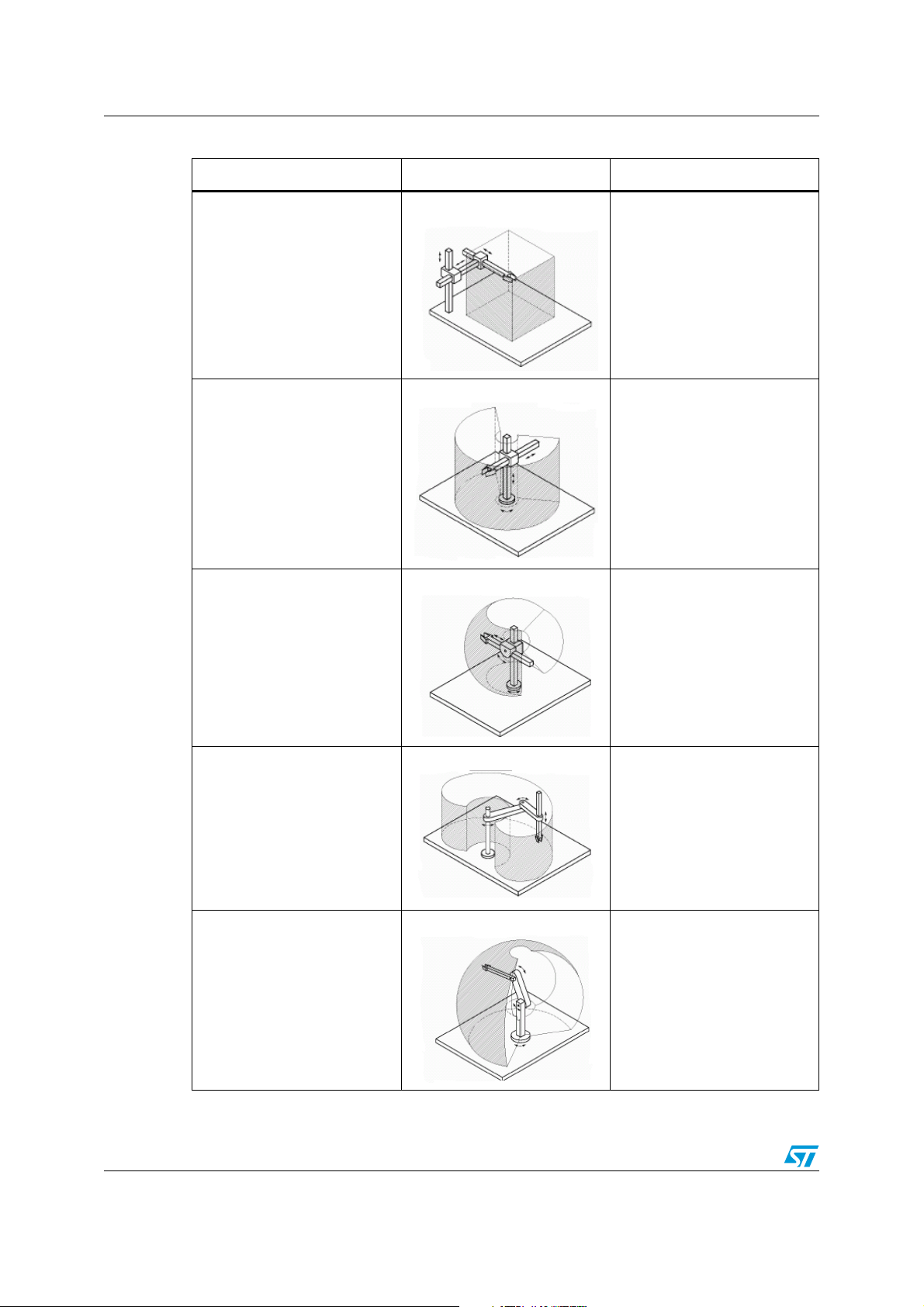
Ta bl e 1 shows a classification of the manipulators accordingly to the type and sequence of

the degrees of mobility of the structure, and of their workspaces.

3/41

An overview on robotics AN2350

Table 1. Open chain manipulators classification

Type Workspace Joints

– Three prismatic joints

Cartesian

Cylindrical

– A Cartesian degree of

freedom corresponds to every
joint

– One revolute joint and two

prismatic joints

– Cylindrical coordinates

Spherical

SCARA

Anthropomorphic

– Two revolute joints and one

prismatic joint

– Spherical coordinates

– Two revolute joints and one

prismatic joint

– Selective Compliance

Assembly Robot Arm

– Three revolute joints
– It is the most dexterous

structure

4/41

AN2350 An overview on robotics

1.1.1 Kinematics analysis

Robot arm kinematics deals with the analytical study of the geometry of motion of a robot
arm with respect to a fixed reference coordinate system as a function of time without regard
to the forces/moments that causes the motion.

Thus, it deals with the analytical description of the spatial displacement of the robot as a
function of time, in particular the relations between the joint space and the position and
orientation of the end-effector of a robot arm.

In kinematics, we consider two issues:

1. Forward analysis: for a given manipulator, given the joint angle vector
q(t)=(q1(t), q2(t), …., qN(t))
and the geometric link parameters, where n is the number of degrees of freedom,
what is the position and orientation of the end-effector with respect to a reference
coordinate system?

2. Inverse analysis: given a desired position and orientation of the end effector and the
geometric link parameters with respect to a reference coordinate system, can the
manipulator reach the desired manipulator hand position and orientation. And if it can,
how many different manipulator configurations will satisfy the same condition?

For serial robots, the forward analysis problem is usually easy and straightforward.
Unfortunately, the inverse analysis problem is of much more interest. For example, in
industrial applications, the end-effector must follow some desired path; then, we need to find
the joint angles for each position in the path.

T

For redundant robots, the inverse kinematics problem has then an infinite number of
solutions. The extra degrees of freedom can then be used for other purposes, for example
for fault tolerance, obstacle avoidance, or to optimize some performance criteria.

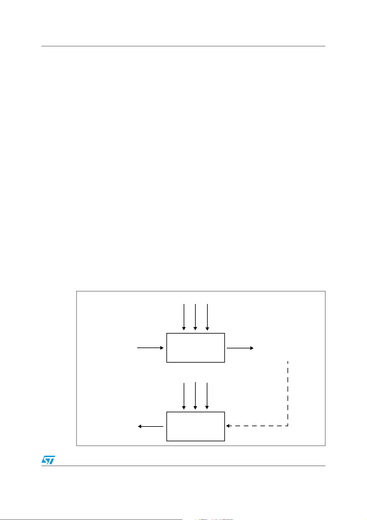
A simple block diagram indicating the relationship between these two problems is shown in
the following figure.

Figure 1. The direct and inverse kinematics problems

Link parameters

Position and

Joint angles
q

(t), q2(t), ..., qN(t)

1

Direct

kinematics

Link parameters

orientation
of the end-effector

Joint angles
q1(t), q2(t), ..., qN(t)

Inverse

kinematics

5/41

An overview on robotics AN2350

Since the links of a robot arm may rotate and/or translate with respect to a reference
coordinate frame, the total spatial displacement of the end-effector is due to the angular
rotations and linear translations of the links.

Denavit and Hartenberg proposed a systematic and generalized approach of utilizing matrix
algebra to describe and represent the spatial geometry of the links of a robot arm with
respect to a fixed reference frame. This method uses a 4 x 4 homogeneous transformation
matrix to describe the relationship between two adjacent rigid mechanical links and reduces
the direct kinematics problem to finding an equivalent 4 x 4 homogeneous transformation
matrix that relates the spatial displacement of the hand coordinate frame to the reference
coordinate frame. These homogeneous transformation matrices are also useful in deriving
the dynamic equation of motion of a robot arm.

In general, the inverse kinematics problem can be solved by several techniques. Most
commonly used approaches are matrix algebraic, iterative, or geometric. A geometric
approach based on both the link coordinate systems and the manipulator configuration has
been used for the industrial wafer handler to which this application note refers.

1.1.2 Singularity

A significant issue in kinematic analysis surrounds so-called singular configurations.
Physically, these configurations correspond to situations where the robot joints have been
aligned in such a way that there is at least one direction of motion (the singular direction[s])
for the end effector that physically cannot be achieved by the mechanism. This occurs at
workspace boundaries, and when the axes of two (or more) joints line up and are
redundantly contributing to an end effector motion, at the cost of another end effector DOF
being lost.

1.2 The industrial wafer handler

This section describes the main characteristics of an industrial wafer handler, used as a
case study for a multiaxial planar manipulator family.

The structure of the manipulator consists of two arms with six joints (one prismatic joint and
five revolute joints) arranged in order to have the motion axes parallel to each other.

The illustration below shows the relation between the axis control and the robot
components.

6/41

AN2350 An overview on robotics

Figure 2. The structure of the wafer handler

Paddle 1

1

H axis

Y axis

Link 2

2

Link 1 Link 1

3

4

5

8

Z axis

6

1. Paddle

2. Link 2

7

3. Link 1

4. Dual Motor Cover

The robot uses 6 electric motors placed as follows:

● Z Axis Motor (Vertical elevation)

● X Axis Motor (Rotation entire robot)

● Dual Motors (Link 2 and Link 1)

Paddle 0

Link 2

A axis

W axis

X axis

5. Torso Beam

6. Robot Body Mounting Flange

7. Chassis Skin

8. Z-Tube

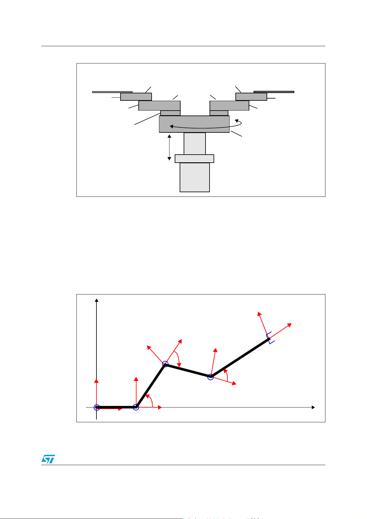
1.2.1 Forward kinematics

Accordingly to the Denavit-Hartenberg convention, an orthonormal cartesian coordinate
system (x

, yi, zi) has been established for each link, in order to characterize the forward

i

kinematics through a D-H homogeneous transformation matrix.

Figure 3. The Denavit Hartenberg convention for one arm

y

y

y

0

1

x

0

y

4

x

4

x

2

y

2

θ

2

x

1

θ

3

y

3

θ

4

x

3

x

Regarding the base coordinates (x
prismatic joint. The origin O

of the base coordinates has been placed at the same height of

0

, y0, z0) , the z0 axis lies along the axis of motion of the

0

7/41

An overview on robotics AN2350

the end effector, when the prismatic joint is at its lower level. The x0 axis lies along the
longitudinal direction of the link 1.

Since all the motion axes are parallel to each other, the origins of the other coordinate
frames have been placed at the same height of the origin O

.

0

The Denavit-Hartenberg parameters are described in the following table:

Table 2. The Denavit Hartenberg parameters for one arm

Link ai [mm] α [rad] di [mm] θ [rad]

1 154 0 d1 0

2 133 0 0 2

3 133 0 0 3

4 215 0 0 4 =- 3/2

In this application note we refer only to one arm, without considering the Z Axis (Vertical
elevation - prismatic joint) and X Axis (Rotation entire robot - revolute joint).

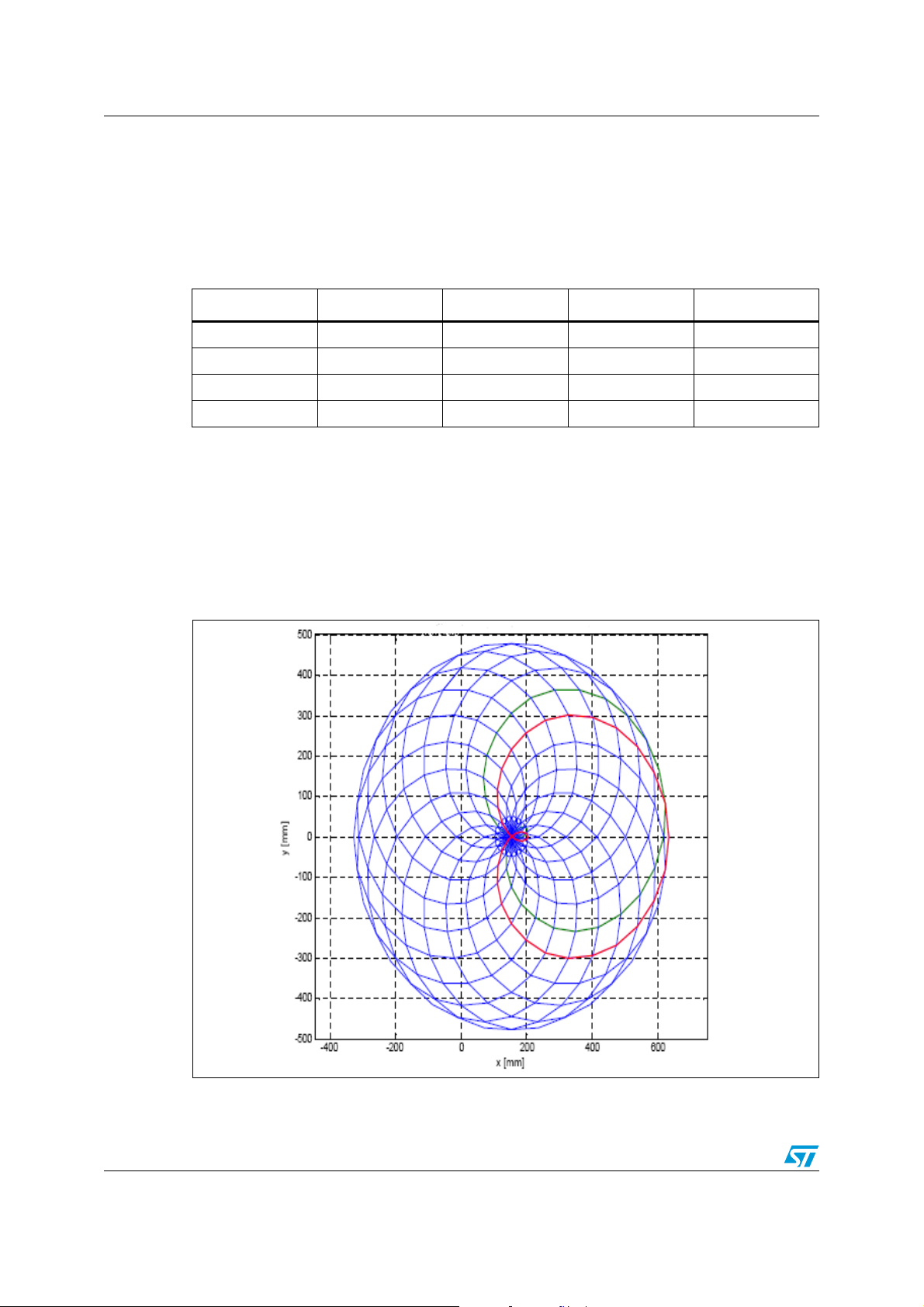
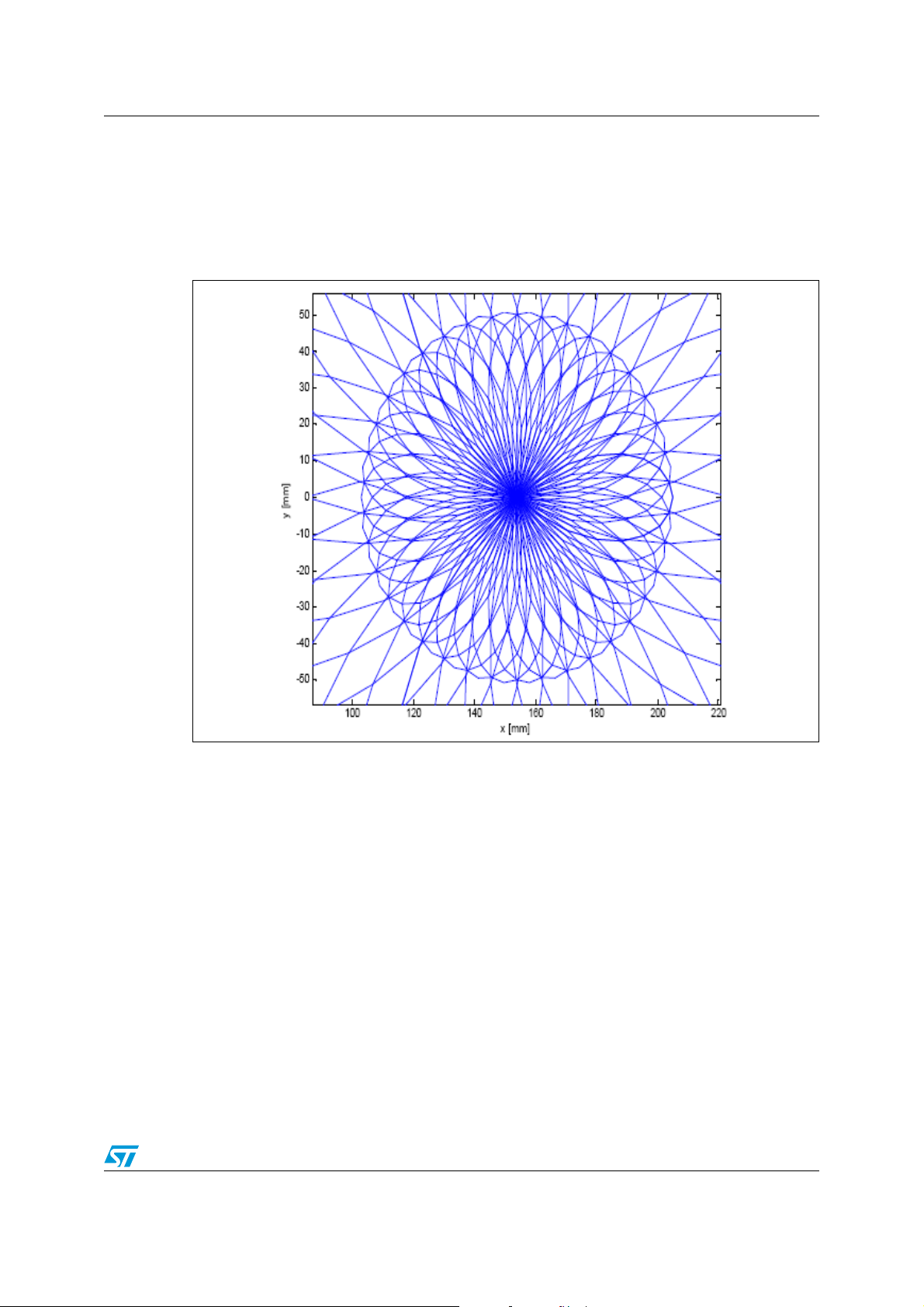
Through a motion simulation it has been possible to obtain the workspace of the
manipulator: for each value of the angle of the joint 1, the joint 2 performs a complete
revolution. As shown in the Figure 4, the workspace has a circular form. Nevertheless
because the joint 3 is under-actuated, there are some regions of the workspace
characterized of different orientations of the end-effector.

Figure 4. The workspace of the wafer handler

8/41

AN2350 An overview on robotics

Out from the circumference, with origin (154 mm, 0 mm) and radius 51 mm, the manipulator
is able to reach a point of the workspace with two possible configurations of the joint
variables; the points inside this circumference are reachable with four possible
configurations of the joint variables as shown in Figure 5.

The center of the workspace is reachable with every orientation.

Figure 5. A detail of the central area of the wafer handler workspace

1.2.2 Inverse kinematics

A geometric approach based on the link coordinate systems and on the manipulator
configuration has been used for the manipulator. Since we refer to the control of only one
arm (link 1 - shoulder, link 2 - elbow), the origin of the base coordinates has been placed in
such way that the z

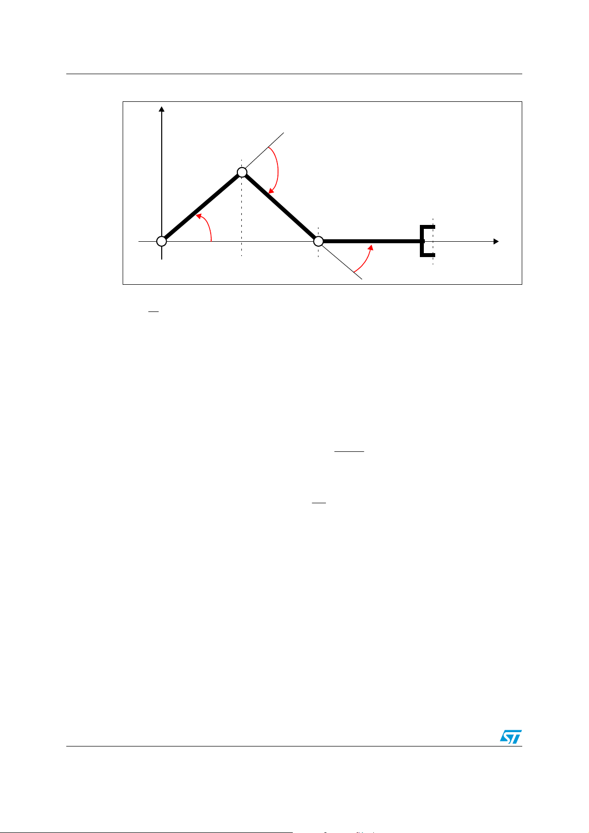
First of all, we consider the manipulator in the configuration described in the following figure.

axis lies along the rotation axis of the revolute joint of the shoulder.

0

9/41

An overview on robotics AN2350

α

Figure 6. The geometric approach for the inverse kinematics

y

α

= -2α’

2

l

1

α

’

1

l

2

1

l

3

/ 2 = α’

x

3

1

x

1

x

2

α

= -

α

3

2

There is a mechanical connection between the link 3 and the link 2, which imposes

2

α

3

Since

. This implies that the joint 3 can not be actuated independently from the joint 2.

−=

2

lll==

21

⎧

=

lx

⎪
⎨
⎪
⎩

cos

'

α

11

'

cos2cos

=+=

cos2

αα

llxx

1212

'

α

+=+=

lllxx

3

1323

From the last equation and from geometric considerations follows:

−

'

α

arccos

=

1

'

αα

−=

2

12

α

α

3

2

2

lx

33

2

l

'

α

=−=

1

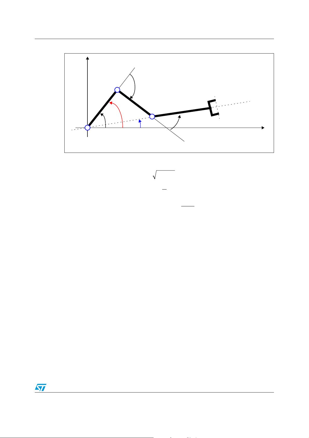
Consider now a rotation of an angle ϕ:

x

10/41

AN2350 An overview on robotics

l

Figure 7. The inverse kinematics after a rotation

y

α

= -2α’

2

l

l

1

α

1

α

’

1

Knowing the position of the end-effector in the workspace, it is possible to deduce its
distance from the origin and the angle ϕ:

2

1

l

3

ϕ

α

= -

α

3

22

yxz

+=

/ 2 = α’

2

Ζ

1

x

α

while
manipulator.

and

2

y

atn

=

ϕ

x

lz

−

arccos

+=

ϕα

1

α

remains the same, because they are independent from the rotation of the

3

3

2

11/41

The SDK-ST10F276 control board AN2350

2 The SDK-ST10F276 control board

2.1 Brief description of the SDK-ST10F276

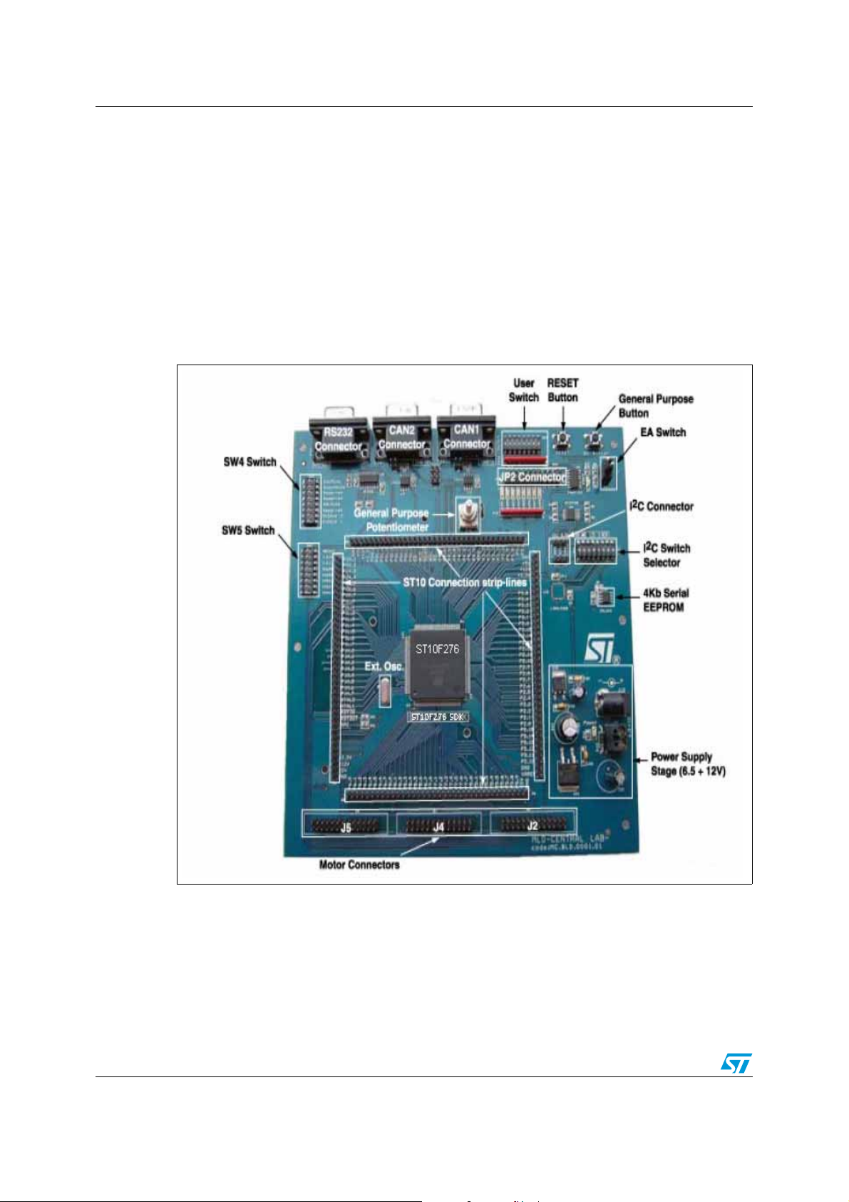
The SDK-ST10F276 is a two-layer, low-cost development board with an ST10F276 16-bit
Embedded Flash Memory Microcontroller (see Figure 8). It is considered a general purpose
application board used for developing advanced motor control solutions and processing
external data (e.g., sensor outputs).

Three dedicated connectors for motion control allow the user to control different kinds of
motors by plugging in external power motor boards.

Figure 8. The SDK-ST10F276 board

12/41

AN2350 The SDK-ST10F276 control board

2.1.1 User Interfaces

The main interfaces used to communicate with the SDK-ST10F276 platform include:

● Two CAN 2.0B interfaces which operate on one or two CAN buses (30 or 2x15

message objects)

● One RS232 connector for serial signal communication with external devices

● One I2C connector for additional external device management

● Three dedicated connectors for motion control (external power motor boards)

● A series of general purpose LEDs and DIP switches

● One potentiometer and a push-button

For the user's convenience, the ST10 I/O pins on the Development board are split into four
main connectors located on each side of the ST10 device

The five general purpose Light Emitting Diodes (LEDs) may be used for end-user
applications.

They can be activated via the JP2 connector, or by using a series of dip switches on the
board.

The potentiometer and push-button may be set in different and independent ways for
general purpose uses.

2.1.2 On board motor control connectors

The SDK-ST10F276 board provides an embedded solution (3 modular connectors) for
power requirements up to 3000W, so they are well-suited for driving motors (e.g. BLDC,
Brushless Direct Current) via an appropriate external motor board. The various power
boards that can be connected to the SDK-ST10F276 are optimized in order to support a
wide variety of advanced motor control applications.

Each of the three power connectors on the SDK-ST10F276 development board has 26 pins
(see Figure 9). When a connector is used with a compatible motor board, the user can drive
motors with the following signals:

● PWM

● Hall Effect sensor/GPIO

● Power/Brake

● Encoder

● Tachometer/Resolver

● Shutdown, and Alarm

13/41

The SDK-ST10F276 control board AN2350

Figure 9. One of the 26 pin connectors of the SDK-ST10F276 board

J2

P8.0
P8.2
P1L.1
P1L.3
P1L.5
P5.15
P5.1
P2.13
P4.0
P4.2

HALL1
HALL3/GPIO1
L1/ENABLE
L2
L3/GPIO4
T2EUD
DINAMO/RES1
EC1
SHUT DOWN
ALARM

GND

11
13
15
17
19
21
23
25

1
3
5
7
9

10
12
14
16
18
20
22
24
26

PWM0

2

HALL2/GPIO2

4

H1/BRAKE

6

H2/FW\REV

8

H3/GPIO3
T2IN
SENSE
RES2
EC2
Set Point ENC

P7.0
P8.1
P1L.0
P1L.2
P1L.4
P3.7
P5.0
P5.2
P2.14
P2.1

+ 12V

1

C5

2

GND

100nF

2.2 ST10F276 16-bit microcontroller - architectural overview

The ST10F276 is a high performance 64MHz 16-bit microcontroller with DSP functions.

ST10F276 architecture combines the advantages of both RISC and CISC processors with
an advanced peripheral subsystem. The following block diagram gives an overview of the
different on-chip components and of the advanced, high bandwidth internal bus structure of
the ST10F276. (see Figure 10).

14/41

AN2350 The SDK-ST10F276 control board

Figure 10. ST10F276 functional block diagram

2.2.1 Basic CPU concepts

The main core of the CPU includes a 4-stage instruction pipeline, a 16-bit arithmetic and
logic unit (ALU) and dedicated SFRs.

Several areas of the processor core have been optimized for performance and flexibility.
Functional blocks in the CPU core are controlled by signals from the instruction decode
logic. The core improvements are summarized below:

● High instruction bandwidth / fast execution

● High function 8-bit and 16-bit arithmetic and logic unit

● Extended bit processing and peripheral control

● High performance branch, call, and loop processing

● Consistent and optimized instruction formats

● Programmable multiple priority interrupt structure

15/41

The SDK-ST10F276 control board AN2350

2.2.2 Memory organization

The memory space of the ST10F276 is organized as a unified memory. Code memory, data
memory, registers and I/O ports are organized within the same linear address space. The
main characteristics are summarized below:

● 512K Bytes of on-chip single voltage Flash memory with Erase/Program controller

● 320K Bytes of on-chip extension single voltage Flash memory with Erase/Program

controller (XFLASH)

● Up to 100K Erase/Program cycles

● Up to 16 MB of linear address space for code and data (5 MB with CAN or I

● 2K Bytes of on-chip internal RAM (IRAM)

● 66K Bytes of on-chip extension RAM (XRAM)

2

C)

2.2.3 On-chip peripheral blocks

The ST10F276 generic peripherals are:

● Two General Purpose Timer Blocks (GPT1 and GPT2)

● Serial channel: Two Synchronous/Asynchronous, two High-Speed Synchronous, I

standard interface

● A Watchdog Timer

● Two 16-channel Capture / Compare units (CAPCOM1 and CAPCOM2)

● A 4-channel Pulse Width Modulation unit and 4-channel XPWM

● A 10-bit Analog / Digital Converter

● Up to 111 General Purpose I/O lines

2

C

Each peripheral also contains a set of Special Function Registers (SFRs), which control the
functionality of the peripheral and temporarily store intermediate data results. Each
peripheral has an associated set of status flags. Individually selected clock signals are
generated for each peripheral from binary multiples of the CPU clock.

2.2.4 Managing Interrupts (hardware)

● 8-channel Peripheral Event Controller for single cycle, interrupt-driven data transfer

● 16-levels of priority for the Interrupt System with 56 sources, and a sampling rate down

to 15.6ns at 64MHz

Note: Refer to the ST10 information listed in the Introduction on page 1 for device details.

16/41

AN2350 Hardware and mechanical equipments

3 Hardware and mechanical equipments

3.1 The Dual DC motor and the power stage

Each arm of the wafer handler is controlled by a dual DC motor (see Figure 17 on page 24);
they are mounted in the same chassis with two armatures which rotate on the same axis
and having concentric drive hubs, as shown in the Figure 12.

Figure 11. The Dual DC motor

The upper armature is connected to the outer drive hub and controls the shoulder (link 1),
while the lower armature is connected to the inner drive hub and controls the elbow (link 2)
through a drive belt with a transmission ratio of 1/2.

17/41

Hardware and mechanical equipments AN2350

Figure 12. The chassis of the dual DC motor

Each DC motor is driven by a monolithic solution (L6205PD) that is a dual full bridge driver.
In order to increase the current capability, the two full bridges inside the driver have been
connected in parallel mode.

A current controller IC (L6506) has been used for both the monolithic drivers in order to
sense the current motor. When the sensed motor current exceeds its current rate, the
current controller disables the power drivers.

Each motor is driven through a PWM signal generated by the microcontroller; the velocity
and the direction of rotation of each DC motor depends on the duty cycle of such signal. For
duty cycles over 50%, the motor moves in one direction, while for duty cycles under 50%,
the motor moves in the opposite direction. For a duty cycle of 50% the motor is stopped.

The driver board has been developed in order to control three links, even if the control
algorithm refers to the control of only one arm (two links).

In the driver board there is also placed a DC/DC converter that generates all the needed
voltages to supply all the circuits and the SDK-ST10F276 board. A detail of the schematic of
the power stage is shown in the following figure.

18/41

AN2350 Hardware and mechanical equipments

Figure 13. A detail of the power stage

19/41

Hardware and mechanical equipments AN2350

3.2 Cables and connectors

On the chassis skin of the wafer handler are present six 15 pin D-SUB male connectors.
Four of them (named A, W, Y, H) are used for the links of the two arms, while the other two,
named X and Z, are used respectively for the torso beam and the Z elevation. The four
harness connectors of the links are located under the torso beam.

The wafer handler is furnished of cables, each of one presents on one side a 15 pin D-SUB
female connector, and on the other side a 25 pin D-SUB female connector. The former is
connected to the wafer handler, while the latter is connected to the driver board. The table
below shows the pins assignment and the related description.

Table 3. The sectors of the absolute encoder

Pin DB15 Connector Pin DB25 Connector Wire Description

1 1 Green

2 2 Orange

33Violet

4 16 Not used

59White

610Grey

7 7 Not used

88Red

9 14 Yellow VREF-

10 15 Blue VREF+

11 19 Not used

12 21 Black

13 23 Not used

14 24 Black (motor) Motor +

15 25 White (motor) Motor -

Incremental encoder
(sin)

Incremental encoder
(cos)

Absolute encoder
(bit b1)

Absolute encoder
(bit b2)

Absolute encoder

)

(bit b

0

2.5V supply for encoder
read head

Ground for encoder
read head

3.3 The encoders and the conditioning circuit

Each joint of the arm of the manipulator has an encoder ring as shown in Figure 14. In this
ring it is possible to identify four sector named A, B, C and D, and the encoder read head.

20/41

AN2350 Hardware and mechanical equipments

Figure 14. The encoder ring of one DC motor

The sectors D, A and B represent the absolute encoder, while the sector C represents the
incremental encoder.

The opaque parts of each sector of the absolute encoder are placed according to a Gray
code, in order to offer absolute position of the link with a resolution of 45 degrees. In this way
it is possible to identify 8 angular positions accordingly to the scheme below, where the
sector D (white wire) represents the most significant bit of the encoder, while the sector A
(grey wire) represents the least significant bit.

Table 4. The sectors of the absolute encoder

Angular position

10000

20011

30113

40102

51106

61117

71015

81004

Sector D

(white wire)

b

2

Sector B

(Violet wire)

b

1

Sector A

(Grey wire)

b

0

Absolute

encoder values

b

2b1b0

In order to capture every transition, in each bit of the absolute encoder has been developed
a logic circuit with NAND ports. A detail of the conditioning circuit for one of the absolute
encoders of the wafer handler is shown in Figure 15. In this way the output of this circuit can
be associated to an external interrupt of the microcontroller, while the output bits of the
absolute encoder can be associated to three GPIOs (General Purpose Input Output) in
order to read its value.

21/41

Hardware and mechanical equipments AN2350

Figure 15. The conditioning circuit for one absolute encoder

The sector C represents the incremental 12-bit encoder, whose outputs are two sinusoidal
signals (available in orange and green wires) shifted to each other by 90 degrees, with an
offset of 2.5 V and a peak-to-peak voltage of 1.1 V.

Since these signals can not be directly managed by the microcontroller, it has been
necessary to develop a conditioning circuit whose outputs are digital signals.

This conditioning circuit for each sinusoidal signal consists of a comparator whose output is
at a logical high level (5 V) every time the input signal level is over 2.5 V, and at logical low
level (0 V) every time the level of the input signal is below 2.5 V. A detail of the conditioning
circuit for one of the incremental encoders of the wafer handler is shown in the following
figure.

22/41

AN2350 Hardware and mechanical equipments

Figure 16. The conditioning circuit for one incremental encoder

Using a trimmer it is possible to have a square wave with a duty cycle of 50% as output.

In this way from the two input sinusoidal signals it is possible to obtain two square signals
shifted each other of 90 degrees, through which it is possible to count 4096 pulses for each
rotation of the joint.

The conditioning circuit presents also a D flip-flop through which it is possible to obtain the
direction of rotation of the joint.

3.4 Schematics of the driver board and the interface board.

The driver board presents three 25 pin D-SUB male connectors to which are plugged the
cables of the wafer handler. In the same board there are 26 pin male connectors, used to
interface the SDK-ST10F276 board through three flat cables.

Figure 17 and Figure 18 show the schematic of the driver board.

23/41

Hardware and mechanical equipments AN2350

Figure 17. Driver board schematic (page 1)

5

25 pin D-SUB male connectors

green_1 orange_1

1 2

violet_1

3 4
5 6

C11_0C10_0

J1

+2.5V

7 8

white_1

9 10
11 12
13 14

+5V

15 16

C4_0

17 18
19
21
23 24

D D

25

motor-_1

CON25A

green_2 orange_2

1 2

J2

violet_2

3 4

C13_0C12_0

5 6

7 8

white_2

9 10
11 12
13 14

+5V

C5_0

15 16

470uF/6.3V

17 18
19
21
23 24
25

motor-_2

CON25A

green_3

1 2

C6_0
470uF/6.3V

+5V

+5V

white_3

+5V

motor-_3

C1_0
100uF

2

IN1

EN_A

B_1

dir_rot_1

IN3

EN_B

B_2

dir_rot_2

IN5

EN_C

B_3

dir_rot_3

J3

violet_3

3 4

5 6

7 8

9 10

11 12
13 14
15 16
17 18
19
21
23 24
25

CON25A

U0

LD25

312

VIN

VOUT

GND

To the interface board

bit0_1_A
abs_enc_1
IN1
bit2_1_A
bit1_1_A
EN_A
bit0_1_
bit1_1_
bit2_1_

J_J1

A_1

1 2

+5V

J_J2

1 2

GND

bit0_2_A
abs_enc_2
IN3
bit2_2_A
bit1_2_A
EN_B
bit0_2_
bit1_2_
bit2_2_

J_J3

A_2

1 2

+5V

J_J4

1 2

GND

bit0_3_A
abs_enc_3
IN5
bit2_3_A
bit1_3_A
EN_C
bit0_3_
bit1_3_
bit2_3_

J_J5

A_3

1 2

+5V

J_J6

1 2

GND

C14_0 C15_0

C C

B B

A A

C7_0

grey_1

470nF/6.3V

1

R1

20

1.6M

22

2

motor+_1

+2.5V
grey_2

C8_0
470uF/6.3V

1

20

R2

22

1.6M

motor+_2

2

orange_3

+2.5V

C9_0

grey_3

470uF/6.3V

1

20

R3

22

+5V

Vcc

1.6M

motor+_3

2

GND

+2.5V

+5V

+2.5V

D1_0
C2_0
100nF

LED

C3_0
470uF/6.3V

2

R0
470

1

J4

1

2

3

4

5

6

7

8

9

10

11

12

13

14

15

16

17

18

Motor_1 ARM_1

19

20

21

22

23

24
25 26

CON26A

GND

J5

1

2

3

4

5

6

7

8

9

10
11

12
13

14
15

16

Motor_2 ARM_1

17

18
19

20
21

22
23

24
25 26

CON26A

GND

J6

1

2

3

4

5

6

7

8

9

10
11

12
13

14
15

16
17

18

Motor_1 ARM_2

19

20
21

22
23

24
25 26

CON26A

GND

5

C9_1 100uF/6.3V

+2.5V

C1_1
100nF

+2.5V

C5_1
100nF

+2.5V

C1_2
100nF

+2.5V

C5_2
100nF

C12_3100uF/6.3V

+2.5V

C1_3
100nF

+2.5V

C5_3
100nF

4

+5V

+5V

+5V

+5V

C3_1 100nF

2

C2_1100nF

R2_1

4.7k

3

U1B

7

+

LM339

green_1

6

-

12

10K

R1_1

U1A

5

+

LM339

orange_1

4

-

10K

R3_1

U1C

9

+

LM339

green_2

8

-

10K

R1_2

U1D

11

+

LM339

orange_2

10

-

10K

R3_2

+5V

C2_3

100nF

8

U2A

3

+

LM393

green_3

2

-

4

10K

R1_3

U2B

5

+

LM393

orange_3

6

-

10K

R3_3

4

U4

1

1

1

5 6

D

U3C

253

CK

+5V

2

1

2

+5V

2

1

14

+5V

2

1

13

+5V

2

1

1

+5V

2

1

7

R4_1

4.7k

3 4

R2_2

4.7k

9 8

R4_2

4.7k

11 10

R2_3

4.7k

1 2

R4_3

4.7k

13 12

GND

74HC14

7 14

74V1G79

+5V

A_1
B_1

dir_rot_1

U3B
74HC14

+5V

U5

A_2

1

D

U3D

253

CK

GND

74HC14

74V1G79

+5V

A_2

B_2

dir_rot_2

U3E
74HC14

+5V

U6

A_3

1

D

U3A

253

GND

CK

74HC14

74V1G79

+5V

U3F

A_3

B_3

dir_rot_3

74HC14

C10_1
22nF

C11_1
22nF

C8_2
22nF

C9_2
22nF

C10_3
22nF

C11_3
22nF

Vcc

Vcc

Vcc

C4_1 100nF

4

Q

J7

1
2
3
4
5

CON5

C4_2 100nF

4

Q

J8

1
2
3
4
5

CON5

C4_3 100nF

4

Q

J9

1
2
3
4
5

CON5

3

+5V

C6_1 100nF

white_1

dir_rot_1A_1

dir_rot_2

dir_rot_3

1 2

U7A
74HC14

bit2_1

7 14

R5_1
12k

violet_1

3 4

U7B
74HC14

bit1_1

R6_1
12k

grey_1

5 6

U7C

R7_1

74HC14

bit0_1

12k

+5V

C6_2 100nF

white_2

1 2

U9A
74HC14

bit2_2

7 14

R5_2
12k

violet_2

3 4

U9B
74HC14

bit1_2

R6_2
12k

grey_2

5 6

U9C

R7_2

74HC14

bit0_2

12k

+5V

C6_3 100nF

white_3

violet_3

grey_3

3

U8A

1 2

74HC14

bit2_3

7 14

R5_3
12k

U8B

3 4

74HC14

bit1_3

R6_3
12k

U8C

5 6

74HC14

R7_3

bit0_3

12k

13 12

11 10

9 8

13 12

11 10

9 8

13 12

11 10

9 8

2

JP2_1

bit2_1_A

12

bit2_1_

U7F
74HC14

JP1_1

bit1_1_A

12

bit1_1_

U7E
74HC14

JP0_1

bit0_1_A

12

bit0_1_

U7D
74HC14

JP2_2

bit2_2_A

12

bit2_2_

U9F
74HC14

JP1_2

bit1_2_A

12

bit1_2_

U9E
74HC14

JP0_2

bit0_2_A

12

bit0_2_

U9D
74HC14

JP2_3

bit2_3_A

12

U8F

bit2_3_

74HC14

JP1_3

bit1_3_A

12

U8E

bit1_3_

74HC14

JP0_3

bit0_3_A

12

U8D

bit0_3_

74HC14

2

+5V

147

1

U10A

21312

74HCT10

3

U10B

bit1_1

456

74HCT10

bit0_1

9

U10C

10118

74HCT10

bit2_1

1

U11A

21312

74HCT10

+5V

147

3

U11B

456

74HCT10

9

U11C

bit1_2

10118

74HCT10

bit0_2

1

U12A

21312

74HCT10

bit2_2

3

U12B

456

74HCT10

+5V

147

9

U12C

10118

74HCT10

1

U13A

bit1_3

21312

74HCT10

bit0_3

3

U13B

456

bit2_3

74HCT10

+5V

147

9

U13C

10118

74HCT10

Title

WAFER HANDLER DRIVER BOARD

Size Document Number Rev

Date: Sheet

C7_1 100nF

C7_2 100nF

C7_3 100nF

C9_3 100nF

1

+5V

C8_1 100nF

147
1
2

U14A

6

74HCT20

4
5

9

10

U14B

8

74HCT20

12
13

+5V

C8_3 100nF

147
1
2

U15A

6

74HCT20

4
5

9

10

U15B
74HCT20

12
13

12Friday, March 31, 2006

1

J_J7

abs_enc_1

12

J_J8

abs_enc_2

12

J_J9

abs_enc_3

12

8

of

24/41

Hardware and mechanical equipments AN2350

Figure 18. Driver board schematic (page 2)

5

100nF SMD 1026

C10_A

IN1

U16A

D D

C C

B B

A A

1 7

IN3

U16B

IN3

3 5

+5V

R0_A
12k 0.25W

R4_A

CW

Spectrol74W 50k

C2_A

2.2nF P5

+24V

U22
L5973D

8 1

12

3

C14

+

2

10uF

4

12

C17

22nF

12

C18

12

220pF

R6

4K7

GND

IN5

IN5

U16C

6 2

Spectrol74W 50k

+5V Vcc

GND

10k 5% 0.25W SMD 1026

IN2IN1

74V2G14

4 8

IN4

74V2G14

4 8

VIN VOUT
INH
SYNC
COMP

VREF

6

10k 5% 0.25W SMD 1026

IN6

74V2G14

+5V

R0_C
12k 0.25W

R4_C

CW

C13

2.2nF P5

R1_A

U17

5
6
7
8

4

1
3
2

+5V

R2_B
20k 1% SMD 1026

R3_B

CW

CW

Spectrol74W 5k

L1 22uH

1 2

21

5

FB

D0
STPS2L25U

GND

7

R1_C

U19

5
6
7
8

4

1
3
2

In1
In2
In3
In4

EN

R/C
Sync
Osc_Out

In1
In2
In3
In4

EN

R/C
Sync
Osc_Out

+5V

20

VCC

L6506

+5V

+5V

20

VCC

L6506

4

C1_A 100nF SMD 1026

11

16

Out1

NC

15

Out2

14

Out3

13

Out4

12

Vsense1

17

Vsense2

18

Vref1

19

Vref2

GND NC

9 10

t=150us

C3_B

68nF SMD 1026

12

R4

12

5K6

+

12

R5
1K8

C1_C 100nF SMD 1026

11

16

Out1

NC

15

Out2

14

Out3

13

Out4

12

Vsense1

17

Vsense2

18

Vref1

19

Vref2

GND NC

9 10

SENSE_A
SENSE_B

68nF SMD 1026

+5V

C15
100uF/6.3V

Sanyo
Poscap

SENSE_C

t=150us

Spectrol74W 5k

12

C16
100nF

C3_C

J10

1
2
3
4

CON4

t=150us

Spectrol74W 5k

JP1

J11

1
2

CON2

+5V

R3_C

50 mils

+5V

R2_A

20k 1% SMD 1026

R3_A

C3_A

C19

100uF/6.3V

100uF/6.3V

passo 50 mils

R2_C
20k 1% SMD 1026

CW

10k 5% 0.25W SMD 1026

+5V

R5_A

EN_A

R6_D

CW

10k 5% 0.25W SMD 1026

+5V

R5_B

EN_B

C20

10k 5% 0.25W SMD 1026

R5_C

+5V

EN_C

3

Kemet Electronics 220nF/100V CER P5

Siemens Matsushita 220nF/100V POLIEST

4.7k 5% 0.25W SMD 1026
R6_A

C9_A

47uF/6.3V

Kemet Electronics 220nF/100V CER P5

Siemens Matsushita 220nF/100V POLIEST

4.7k 5% 0.25W SMD 1026
R6_B

C9_B

R6_ER6_F

47uF/6.3V

Kemet Electronics 220nF/100V CER

Siemens Matsushita 220nF/100V POLIEST

4.7k 5% 0.25W SMD 1026

R6_C

C9_C

47uF/6.3V

POWER SUPPLY-24VDC

N.C.

Contact N.A.

DB9 female
connector

P2

6

IN1A

7

IN2A

14

IN1B

15

IN2B

5

ENA

16

ENB

SENSE_A

C8_A

470pF SMD 1026

6

IN1A

7

IN2A

14

IN1B

15

IN2B

5

ENA

16

ENB

SENSE_B

C8_B

470pF SMD 1026

6

IN1A

7

IN2A

14

IN1B

15

IN2B

5

ENA

16

ENB

SENSE_C

C8_C

470pF SMD 1026

CN1

2
1

+24V

1
6
2
7
3
8
4
9
5

C4_A

1

10

11

20

GND

GND

GND

GND

1k 1%

C4_B

1

10

11

20

GND

GND

GND

GND

1k 1%

C4_C

1

10

11

20

GND

GND

GND

GND

1k 1%

1 2

R8

47K

1 2

R9

2.2K
Panasonic FA 100uF/63V P5

R12_A

R12_B

R12_C

C5_A

17

VBOOT

C5_B

17

VBOOT

C5_C

17

VBOOT

D2

2

Siemens Matsushita 10nF/100V CER

4

L6205PD

SENSEB

SENSEA

8

13

0.22 Ohm 2W 1%

R8_A

D1_B1N4148

Siemens Matsushita 10nF/100V CER

4

L6205PD

SENSEB

SENSEA

8

13

0.22 Ohm 2W 1%

R8_B

D1_C1N4148 D2_C1N4148

Siemens Matsushita 10nF/100V CER

4

L6205PD

SENSEB

SENSEA

8

13

0.22 Ohm 2W 1%

R8_C

Vin

1N4007

M1

C12

R7_A

VCP

U18

R7_B

VCP

U20

R7_C

VCP

U21

K1

D2_A1N4148D1_A1N4148

100 ohm SMD 1026

C6_A

D2_B1N4148

100 ohm SMD 1026

C6_B

100 ohm SMD 1026

C6_C

3

6
1

2

RELAY DPDT

1

C7_A

470uF/35V

19

2

VSB

VSA

motor+_1

9

OUT1A

3

OUT2A

12

OUT1B

18

OUT2B

C7_B

470uF/35V

19

2

VSB

VSA

9

OUT1A

3

OUT2A

12

OUT1B

18

OUT2B

C7_C

470uF/35V

19

2

VSB

VSA

9

OUT1A

3

OUT2A

12

OUT1B

18

OUT2B

4

+24V

5
8

7

+24V

D1
LED

2

R7
1K

1

motor-_1

+24V

motor+_2
motor-_2

motor+_3
motor-_3

CN2

2
1

AUXILIARY-24VDC

motor+_1
motor-_1

motor+_2
motor-_2

motor+_3
motor-_3

5

4

To avoid electromagnetic interference, all the signals have been shielded. For this reason an
interface board with three 26 pin female shielded connectors has been developed, in order
to be plugged in the male connectors of the SDK-ST10F276 board. The schematic of the
interface board is shown below.

25/41

3

2

1

Hardware and mechanical equipments AN2350

Figure 19. The interface board schematic

26/41

Control algorithm AN2350

4 Control algorithm

4.1 Motion and path planning

Path planning problems generally involve computing a continuous sequence (a path) of
configurations (generalized coordinates) between an initial configuration (start) and a final
configuration (goal) respecting certain constraints.

The term motion planning is usually distinguished from path planning in that the computed
path is parameterized by time (i.e. a trajectory). The consideration of time is often important
for problems requiring time-parameterized solution trajectories.

The aim of the motion planning is to generate the inputs of the motion control system in
order to ensure the correct execution of the planned trajectory by the manipulator.

The path planning can be realized in the joint space or in the workspace. The latter has
been used in this work according to the scheme of the following figure.

Figure 20. General scheme for the path planning

As can be seen, all the reference points necessary to the control of the desired trajectory
are calculated off-line. The trajectory planning algorithm generates a temporal sequence of
variables that specify the position and orientation of the end-effector in the workspace.
Because the control of the manipulator is realized as control of the joints, from this
sequence of variables it is necessary to perform the kinematics inversion to build a
sequence of variables in the joint space. These joint variables must be opportunely
converted in incremental encoder pulses, because the position closed loop control is
performed on the feedback of the incremental encoders of the two joints.

The path planning method used in this work is the straight-line motion. In this method the
end-effector of the robot travels in a straight line between the start and stop points, using a
trapezoidal velocity profile, in which the motion controller must command the motor driver to

27/41

Control algorithm AN2350

gradually ramp-up the motor velocity, until it reaches the desired speed and then, gradually
ramp-down it until it stops after the task is complete, as shown in Figure 21:

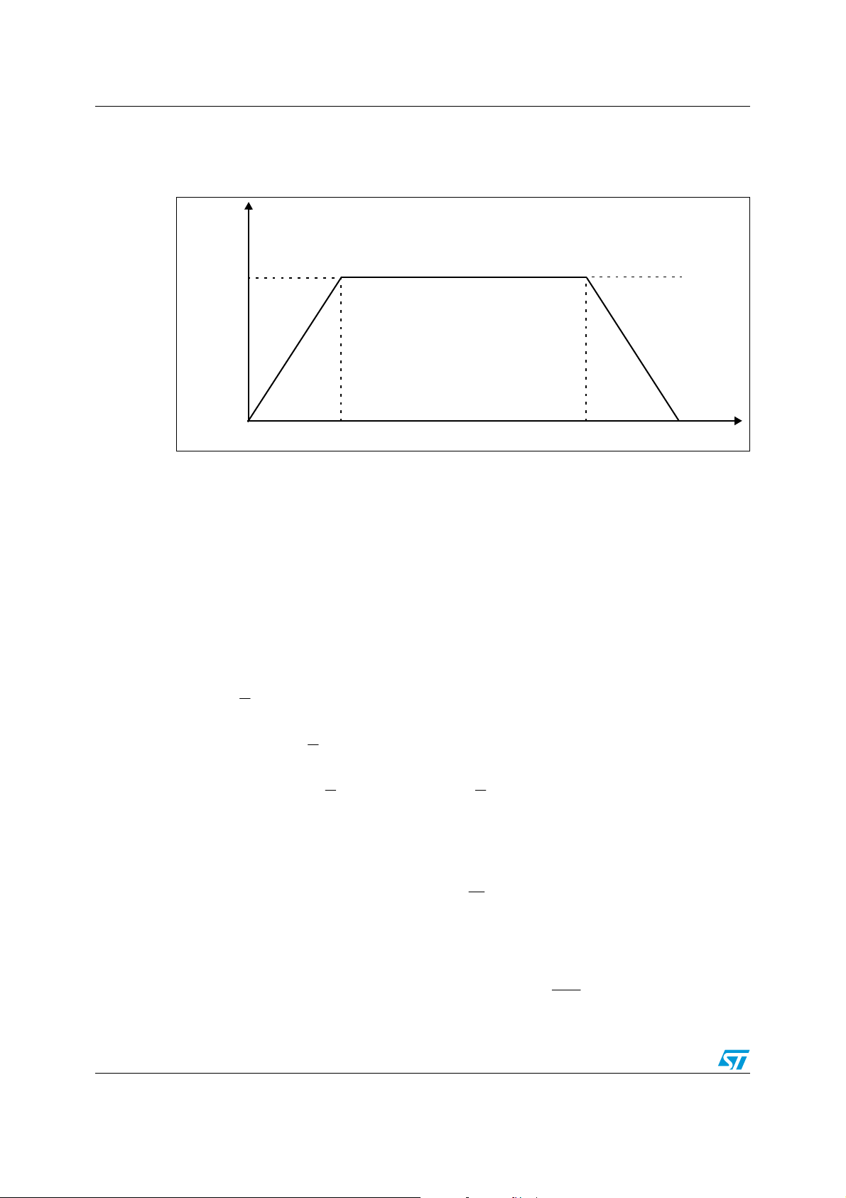
Figure 21. Example of trapezoidal velocity profile

Motor
Speed

The trapezoidal velocity profile is analytically expressed as follows:

where t
trajectory, and is the time slot during which the end effector moves at desired
speed v

Integrating it respect to the time, it is possible to obtain the function that describes the space
covered in the workspace.

Accelerate Cruising speed

t

1

at

⎧
⎪

=

)(

tv

⎨

c

⎪

c

⎩

is the time slot for the ramp-up, t3 is the total time for the execution of the entire

1

(also called the cruising speed).

c

)(t

tt −=

132

TimeStart

)(t )(

Decelerate

Stop

t

2

<≤

tt0

1

−<≤

)( t

tttv

131

<≤−+−−

ttttttav

31313

t

3

1

⎧

2

at

⎪

2

⎪
⎪

=

)(

ts

⎨

c

⎪
⎪
⎪

⎩

The time t
a (that represent the known parameters)

and the total time t
stop point as follows:

28/41

can be obtained from the knowledge of the cruising speed and the acceleration

1

1

)t-(t

1

2

2

1

)2(

can be obtained from the distance s

3

2

113

2

cc

<≤

tt0

1

−<≤+

)(t at

tttv

131

1

)(at

2

v

c

=1t

2

1313

<≤−+−+−++−

)(t )t-a(t

tttttttvttv

313

a

between the start point and the

max

s

tvtvts

cc

t )(s t

max

+=⇒−==

3133max

1

v

c

Control algorithm AN2350

=

−

Now follows the algorithm used for the motion planning in order to build a trajectory table
whose points (as joint variables after the reversal kinematics and expressed as incremental
encoder pulses) are given as inputs to the PID control interrupt service routine every T
(fixed in 20 ms).

),(

Let the coordinates of the start point and the coordinates of the stop
point, v
possible to obtain the time t

yx ),(22yx

11

the cruising speed and a the acceleration. From the previous equations it is

c

and the time t3 , where:

1

2

12max

2

)()( yyxxs −+−=

12

,

R

Consider as the generic straight-line that intersect the two points and

, where

),(

yx

22

is the angular coefficient and

is the intersection with the Y axis.

It is possible that the cruising speed it is not compatible with the imposed acceleration and
the distance to cover: this implies that the velocity profile is not trapezoidal. For this reason a
convergent loop procedure has been developed (shown in the following scheme) that
redefines the values of t

cmxy +

, vc , and t3 .

1

),(

yx

11

yy

m

=

⎛

1

⎜

yyc

−+=

⎜

2

⎝

21

12

−

xx

12

⎞

xxyy

+−

))((

1212

⎟

xx

−

12

⎟

)(

⎠

29/41

Control algorithm AN2350

Figure 22. Convergent loop procedure for a trapezoidal velocity profile

Acceleration a

Cruising Speed v

Max Distance S

≥ t3 / 2

t

1

max

c

t

N

= vc / a

1

t

= t1 + s

3

max

/ v

c

Y

t1 = t3 / 2 - T

R

vc = t1 . a

t

= t1 + s

3

At the generic sampling time T
is equal to ; so the point of the trajectory to reach in a straight-line motion
at time T

in the workspace, can be obtained resolving the following system:

i

)(

Tss =

ii

, the covered distance, accordingly to the previous equation,

i

⎧
⎨
⎩

/ v

max

c

),( yx

2

i

2

1

+=

cmxy

2

−+−=

yyxxs

)()(

1

Knowing it is possible to obtain the corresponding joint variables

),( yx

inverse kinematics equations. These joint variables must be opportunely converted in
incremental encoder pulses, because the position closed loop control is performed on the
feedback of the incremental encoders of the two joints.

During the trajectory planning it is very important that the manipulator avoids crossing the
kinematics singularities of the accessible workspace since they could make the continuation
of the trajectory impossible.

For this wafer handler, these singularities are distributed along the circle with radius 51 mm
and center in the origin of the base coordinates. The motion singularity appears only when
the manipulator, during the motion, crosses the point of the circle assuming a configuration
with the arms aligned, as shown in the following figure.

30/41

α

and α2 with the

1

Control algorithm AN2350

Figure 23. The kinematics singularities of the wafer handler during motion

This problem happens only when the manipulator moves along a straight-line passing
through the origin (c = 0) and when the abscissas and are of opposite sign. The

x

1

x

2

problem has been solved making a change of orientation in the origin in order to cross the
kinematics singularity with an alternative configuration as shown in Figure 24.

Figure 24. How to solve the kinematics singularities during the motion

31/41

Control algorithm AN2350

As shown in the figure above, the trajectory in this case is made of three tracts.

● A straight-line tract with a trapezoidal velocity profile that brings the end-effector from

the start point to the origin .

● A change of the configuration in which the entire arm is rotated of 180°. We can see

how the position of the end-effector remains the same while its orientation is changed.

● A straight-line tract with a trapezoidal velocity profile that brings the end-effector from

the origin to the stop point .

Figure 25. Motion path planning scheme to avoid singularities

),(11yx )0,0(

)0,0(

),(22yx

Start point (x1, y1)

Stop point (x2, y2)

Motion path planning

Straight-line motion

(x1,y1) ⇒ (x2,y2)

Trajectory table as

encoder pulses

N

c=0

Y

Y

sign(x1)

=

sign(x2)

Straight-line motion

(x1,y1) ⇒ (0,0)

Configuration change

180° rotation

Straight-line motion

(0,0) ⇒ (x2, y2)

4.2 PID position control algorithm

The points of the trajectory table have to be given as input one by one to the control
algorithm every T
routine (ISR) is performed every 1ms.

The trajectory table is composed of two arrays; one for the shoulder (shoulder_array[ ]) and
one for the elbow (elbow_array[ ]), obviously of the same dimension.

The control ISR has been associated to the compare unit CC2, while the scanning of the
trajectory table has been associated to the compare unit CC3.

The incremental encoders of the shoulder and the elbow have been associated to the GPT1
timers T2 and T4, respectively, used in incremental interface mode.

32/41

, that has been fixed in 20 ms, while the PID control interrupt service

R

Control algorithm AN2350

To ensure that the point has been reached, a check on the error has been performed in a
such way that if the total error (as sum of the error of the shoulder and of the elbow) is higher
than a fixed value (MAX_ERR_POS=150 ) no new point is passed. The figures below show
the general schemes for the control algorithm ISR and for the scanning of the trajectory
table.

The variables sh_pulses_desired, elb_pulses_desired, total_error, index, flag_error are
global variables.

33/41

Control algorithm AN2350

Figure 26. PID position control ISR

Reload of Compare unit CC2

and Reset errors

T2

sh_pulses_desired

T4

elb_pulses_desired

Encoder feedback for

shoulder and error

computation

error_shoulder

PID_Position_Control

for the shoulder

P

, Ish, D

sh

sh

Encoder feedback for

elbow and error

computation

error_elbow

PID_Position_Control

for the elbow

P

, I

elb

, D

elb

elb

Compute total error as

abs(error shoulder)

+

abs(error_elbow)

PW0

(max 90% - min 10%)

or

(max 65% - min 35%)

PW1

(max 90% - min 10%)

or

(max 65% - min 35%)

34/41

total_error

>

MAX_ERR_POS

Y

flag_error =1

N

flag_error =0

Control algorithm AN2350

Figure 27. Trajectory table scanning ISR

Reload of compare unit CC3

index++;

Start Timer T6

if(flag_error)

Y

Exit

N

sh_pulses_desired=shoulder_array[index];

elb_pulses_desired=elbox_array[index];

Stop and Reset Timer T6

Redefine upper and lower PWM limit

(min PWM=10% - maw PWM=90%)

To avoid oscillations due to external events that could change the motion direction, an
additional control algorithm is performed using the ISR associated to timer T6, every 200ms.
This implies that if for 10 times no new reference point is given to the control ISR, in the ISR
associated to timer T6 the values of PWM are strongly limited until the stop point is reached,
drastically reducing the oscillations.

4.3 Homing procedure

The Homing procedure is the most important task a manipulator must execute at start-up. It
can be seen as a calibration and alignment phase to the end of which, the manipulator is in
a configuration that allows it to perform the other tasks correctly.

For the wafer handler there are many possible home alignment configurations according to
the position in which it is placed and to the tasks that it must execute.

For our purpose a homing position has been chosen in which the controlled arm is
completely extended. This configuration corresponds to an end effector position at the point
of coordinates (481,0).

The homing procedure has been performed through the absolute encoder feedback of the
two links, using three GPIOs (one for each bit of the absolute encoder) and one Capture pin
(to capture every transition in each bit), for each link. The homing procedure is performed
first for the shoulder and then for the elbow. The figures below show the value of the
absolute encoder for the shoulder and for the elbow.

35/41

Control algorithm AN2350

Figure 28. Values of the absolute encoder for the shoulder

X

Homing position

7

6

2

3

Figure 29. Values of the absolute encoder for the elbow

7

5

5

4

0

1

X

Homing position

6

2

Y

Y

4

Values in the different sectors represent the decimal value of the bits of the absolute
encoder.

As we can see, the homing position for the shoulder is characterized by a transition between
the sectors with values 7 and 5, while the elbow by a transition between the sectors with
values 7 and 6.

At the startup of the homing procedure the absolute encoder of the shoulder is read and the
ISR associated to the Capture unit CC16 is enabled. Accordingly to the sector in which the
shoulder is positioned, the shoulder is moved with a fixed PWM. Every time there is a
transition, in the ISR the absolute encoder is read. If the transition is right, then the motor of
the shoulder is stopped (PWM=50%) and the timer T2 of the incremental encoder is reset.
This value is then passed to the control algorithm.

36/41

3

0

1

bbb

012

Control algorithm AN2350

Now the shoulder is controlled in its home position, the same procedure is executed for the
elbow, using the Capture unit CC22. The control of the shoulder ensures that during the
home procedure for the elbow there's no movement of the shoulder.

The scheme below shows the homing procedure.

Figure 30. The homing procedure

Read Absolute Encoder

of the shoulder and

enable interrupt CC16

Read Absolute Encoder

for the shoulder

ISR for the

shoulder

while(!home_position_sh)

{

Move shoulder with fixed PWM

}

Stop the shoulder

Reset incremental encoder

of the shoulder (T2)

Enable interrupt for control

algorithm, and disable

interrupt CC16

sh_pulses_desired

Read Absolute Encoder

of the elbow and enable

interrupt CC22

while(!home_position_elb)

{

Move elbow with fixed PWM

}

This is the right

transition?

Y

home_position_sh=true;

Exit

Read Absolute Encoder

for the elbow

This is the right

transition?

N

Control

Algorithm

ISR for the

elbow

N

Stop the elbow

Reset incremental encoder

of the elbow (T4)

Disable interrupt CC22

elb_pulses_desired

37/41

Y

home_position_elb=true;

Exit

Control algorithm AN2350

4.4 Teach and Repeat procedure

Robots are mainly programmed using a technique known as teach and repeat. Using this
technique the control system stores internal joint poses specified by a human operator and
then recalls them in sequence to execute a task. In this way it is possible to store complex
trajectories allowing the robot can execute them with a good reliability and repeatability.

During the teach phase the control of the manipulator is disabled and the human operator
can move the arm as he wants. With a periodic task of 20 ms (associated to the Compare
Unit CC8 and the timer T0) the value of the incremental encoders of the two joints (the
shoulder and the elbow) are stored in the two corresponding arrays: shoulder_array_teach[]
and elbow_array_teach[]. The teach phase duration depends on the size of the two arrays.
Using 3 KByte of the XRAM2 for each array, it is possible to store a trajectory of 30 seconds.
In the repeat phase the couple of points of the two arrays are passed to the control algorithm
as explained before, as well the scanning of the two arrays. The scheme for teach and
repeat procedure is shown in the figure below.

38/41

Control algorithm AN2350

Figure 31. The teach and repeat procedure

Teach Procedure

Execute homing procedure

Stop the control

Stop the motors (PWM=50%)

Reset timer T0

Enable interrupt CC8

index=0;

Start timer T0

while index<1500

Disable interrupt CC8

Stop timer T0

ISR for teach

Reload of Compare unit

CC8

Read Incremental

Encoder for the shoulder

(T2)

Store T2 in

shoulder array teach[]

Read Incremental

Encoder for the elbow

(T4)

Store T4 in

elbow-array-teach[]

index++

Execute homing procedure

Reset Timer T0

Enable interrupts CC2 and CC3

Start timer T0

elbow_array_teach[]

shoulder_array_teach[]

39/41

Repeat Procedure

Control

Algorithm

Revision history AN2350

5 Revision history

Table 5. Document revision history

Date Revision Changes

30-Nov-2006 1 Initial release.

40/41

AN2350

Please Read Carefully:

Information in this document is provided solely in connection with ST products. STMicroelectronics NV and its subsidiaries (“ST”) reserve the
right to make changes, corrections, modifications or improvements, to this document, and the products and services described herein at any
time, without notice.

All ST products are sold pursuant to ST’s terms and conditions of sale.

Purchasers are solely responsible for the choice, selection and use of the ST products and services described herein, and ST assumes no
liability whatsoever relating to the choice, selection or use of the ST products and services described herein.

No license, express or implied, by estoppel or otherwise, to any intellectual property rights is granted under this document. If any part of this
document refers to any third party products or services it shall not be deemed a license grant by ST for the use of such third party products
or services, or any intellectual property contained therein or considered as a warranty covering the use in any manner whatsoever of such
third party products or services or any intellectual property contained therein.

UNLESS OTHERWISE SET FORTH IN ST’S TERMS AND CONDITIONS OF SALE ST DISCLAIMS ANY EXPRESS OR IMPLIED
WARRANTY WITH RESPECT TO THE USE AND/OR SALE OF ST PRODUCTS INCLUDING WITHOUT LIMITATION IMPLIED
WARRANTIES OF MERCHANTABILITY, FITNESS FOR A PARTICULAR PURPOSE (AND THEIR EQUIVALENTS UNDER THE LAWS
OF ANY JURISDICTION), OR INFRINGEMENT OF ANY PATENT, COPYRIGHT OR OTHER INTELLECTUAL PROPERTY RIGHT.

UNLESS EXPRESSLY APPROVED IN WRITING BY AN AUTHORIZED ST REPRESENTATIVE, ST PRODUCTS ARE NOT
RECOMMENDED, AUTHORIZED OR WARRANTED FOR USE IN MILITARY, AIR CRAFT, SPACE, LIFE SAVING, OR LIFE SUSTAINING
APPLICATIONS, NOR IN PRODUCTS OR SYSTEMS WHERE FAILURE OR MALFUNCTION MAY RESULT IN PERSONAL INJURY,
DEATH, OR SEVERE PROPERTY OR ENVIRONMENTAL DAMAGE. ST PRODUCTS WHICH ARE NOT SPECIFIED AS "AUTOMOTIVE
GRADE" MAY ONLY BE USED IN AUTOMOTIVE APPLICATIONS AT USER’S OWN RISK.

Resale of ST products with provisions different from the statements and/or technical features set forth in this document shall immediately void
any warranty granted by ST for the ST product or service described herein and shall not create or extend in any manner whatsoever, any
liability of ST.

ST and the ST logo are trademarks or registered trademarks of ST in various countries.

Information in this document supersedes and replaces all information previously supplied.

The ST logo is a registered trademark of STMicroelectronics. All other names are the property of their respective owners.

© 2006 STMicroelectronics - All rights reserved

STMicroelectronics group of companies

Australia - Belgium - Brazil - Canada - China - Czech Republic - Finland - France - Germany - Hong Kong - India - Israel - Italy - Japan -

Malaysia - Malta - Morocco - Singapore - Spain - Sweden - Switzerland - United Kingdom - United States of America

www.st.com

41/41