

Page 1
SPSS® Trends 13.0
Page 2

For more information about SPSS®software products, please visit our Web site at http://www.spss.com or contact
SPSS Inc.
233 South Wacker Drive, 11th Floor
Chicago, IL 60606-6412
Tel: (312) 651
Fax: (312) 651-3668
SPSS is a registered trademark and t he other product names are the t rademarks of SPSS Inc. for its proprietary computer
software. No m
the trademark and license rights in the software and the copyrights in the published materials.
The SOFTWARE and documentation are provided with RESTRICTED R IGHTS. Use, duplication , or disclosure by the
Governmentis
clause at 52.227-7013. Contractor/manufacturer is SPSS Inc., 233 South Wacker Drive, 11th Floor, Chicago, IL 60606-6412.
General notice: Other product names mentioned herein are used for identification purposes only and may be trademarks of
their respec
TableLook is a trademark of SPSS Inc.
Windows is a registered trademark of Microsoft Corporation.
DataDirect, D
Portions of this product were created using LEADTOOLS © 1991–2000, LEAD Technologies, Inc. ALL RIGHTS RESERVED.
LEAD, LEADTOOLS, and LEADVIEW are registered trademarks of LEAD Technologies, Inc.
Sax Basic is a t
All rights reserved.
Portions of this product were based on the work of the FreeType Team (http://www.freetype.org).
A portion of th
software is provided “as is,” without express or implied warranty.
A portion of the SPSS software contains Sun Java Runtime libraries. Copyright © 2003 by Sun Microsystems, Inc. All rights
reserved. The
licensed from IBM and are available at http://oss.software.ibm.com/icu4j/.
SPSS Trends™ 13.0
Copyright © 20
All rights reserved.
Printed in the United States of America.
No part of this p
electronic, mechanical, photocopying, recording, or otherwise, without the prior written permission of the publisher.
1234567890 07060504
ISBN 1-56827-
-3000
aterial describing such software may be produced or distributed without the written permission of the owners of
subject to restrictions as set forth in subdivision (c) (1) (ii) of The Rights in Technical Data and Computer Software
tive companies.
ataDirect Connect, INTERSOLV,and SequeLink are registered trademarks of DataDirect Technologies.
rademark of Sax Software Corporation. Copyright © 1993–2004 by Polar Engineering and Consulting.
e SPSS software contains zlib technology. Copyright © 1995–2002 by Jean-loup Gailly and Mark Adler. The zlib
Sun Java Runtime libraries include code licensed from RSA Security, Inc. Some portions of the libraries are
04 by SPSS Inc.
ublication may be reproduced, stored in a retrieval system, or transmitted, in any form or by any means,
352-5
Page 3

Preface
SPSS 13.0 is a comprehensive system for analyzing data. The Trends optional
add-on mod
The Trends add-on module must be used with the SPSS 13.0 Base system and is
completely integrated into that system.
Installation
To install the Trends add-on module, run the License Authorization Wizard using the
authorization code that you received from SPSS Inc. For more information, see the
installa
Compatibility
SPSS is designed to run on many computer systems. See the installation instructions
that cam
requirements.
ule provides the additional analytic techniques described in this manual.
tion instructions supplied with the SPSS Base system.
e with your system for specific information on minimum and recommended
Serial N
Your ser
this serial number when you contact SPSS Inc. for information regarding support,
payment, or an upgraded system. The serial number was provided with your Base
system
Customer Service
If you have any questions concerning your shipment or account, contact your local
office
your serial number ready for identification.
umbers
ial number is your identification number with SPSS Inc. You will need
.
, listed on the SPSS Web site at http://www.spss.com/worldwide. Please have
iii
Page 4

Training Seminars
SPSS Inc. provides both public and onsite training seminars. All seminars feature
hands-on workshops. Seminars will be offered in major cities on a regular basis. For
more informa
tion on these seminars, contact your local office, listed on the SPSS
Web site at http://www.spss.com/worldwide.
Technical S
The service
upport
s of SPSS Technical Support are available to registered customers.
Customers may contact Technical Support for assistance in using SPSS or for
installation help for one of the supported hardware environments. To reach Technical
Support, s
ee the SPSS Web site at http://www.spss.com, or contact your local office,
listedontheSPSSWebsiteathttp://www.spss.com/worldwide.Bepreparedto
identify yourself, your organization, and the serial number of your system.
Additional Publications
Additional copies of SPSS product manuals may be purchased directly from SPSS
Inc. Visit the SPSS Web Store at http://www.spss.com/estore, or contact your local
SPSS offi
ce, listed on the SPSS Web site at http://www.spss.com/worldwide.For
telephone orders in the United States and Canada, call SPSS Inc. at 800-543-2185.
For telephone orders outside of North America, contact your local office, listed
on the SP
SS Web site.
The SPSS Statistical Procedures Companion, by Marija Norušis, has been
published by Prentice Hall. A new version of this book, updated for SPSS 13.0, is
planned
.TheSPSS Advanced Statistical Procedures Companion, also based on SPSS
13.0, is forthcoming. The SPSS Guide to Data Analysis forSPSS13.0isalsoin
development. Announcements of publications available exclusively through Prentice
Hall wi
your home country, and then click
ll be available on the SPSS Web site at http://www.spss.com/estore (select
Books).
Tel l Us
Your co
Your Thoughts
mments are important. Please let us know about your experiences with SPSS
products. We especially like to hear about new and interesting applications using
the SPSS system. Please send e-mail to [email protected] or write to SPSS Inc.,
iv
Page 5

Attn.: Director of Product Planning, 233 South Wacker Drive, 11th Floor, Chicago,
IL 60606-6412.
About This Manual
This manual documents the graphical user interface for the procedures included in
the Trends add-on module. Illustrations of dialog boxes are taken from SPSS for
Windows. Di
alog boxes in other operating systems are similar. Detailed information
about the command syntax for features in this module is provided in the SPSS
Command Syntax Reference, available from the Help menu.
Contacting SPSS
If you would like to be on our mailing list, contact one of our offices, listed on our
Web site at http://www.spss.com/worldwide.
v
Page 6

Page 7

Contents
Part I: User
's Guide
1Overview 1
TimeSeriesAnalysis........................................... 2
ReasonsforAnalyzingTimeSeries ............................ 2
A Model-B
HowTrendsCanHelp.......................................... 4
ModelIdentification........................................ 4
Parameter
Diagnosis ............................................... 6
2TrendsPr
Defining
Data Tran
New Serie
Historic
Reusing M
Changing
Performa
alandValidationPeriods ................................. 9
uildingStrategy................................... 3
Estimation ...................................... 5
ocedures Common Features 7
TimeSeriesData....................................... 7
sformations.......................................... 7
sNames............................................ 8
odels............................................. 10
SettingswithCommandSyntax.......................... 11
nceConsiderations ................................... 12
3 Exponential Smoothing 15
Custom E
xponentialSmoothingModels ........................... 17
vii
Page 8

ExponentialSmoothingParameters .............................. 18
SavingPredictedValuesandResiduals ........................... 20
EXSMOOTHCommandAdditionalFeatures......................... 21
4 Autoregres
AutoregressionOptions ....................................... 25
SavingPredictedValuesandResiduals ........................... 27
Autoregression Performance and Embedded Missing Data. . . . . . . . . . . . . 28
AREGCommandAdditionalFeatures.............................. 28
sion 23
5ARIMA 31
ARIMA Opt
Saving Pr
ARIMA Per
ARIMA Com
ions.............................................. 34
edictedValuesandResiduals ........................... 36
formanceandEmbeddedMissingData................... 37
mandAdditionalFeatures ............................ 38
6 Seasonal Decomposition 39
Seasona
SEASON C
lDecompositionSave.................................. 41
ommandAdditionalFeatures........................... 41
7 Spectral Plots 43
SPECTR
ACommandAdditionalFeatures........................... 46
viii
Page 9

Part II: Exa
mples
8 Exponential Smoothing 49
Using Expo
RelatedProcedures.......................................... 90
RecommendedReadings ...................................... 90
nential Sm oothing to Predict Future Sales . . . . . . . . . . . . . . . . . 49
Prelimina
UnderstandingYourData................................... 50
Building and Analyzing Exponential Smoothing Models . . . . . . . . . . . . 53
Test i ng t h e
UsingtheModeltoPredictFutureSales ....................... 84
Summary............................................... 89
9 Autoregre
Determining Significan t Predictors in the Presence of Autocorrelation . . . . 91
Preliminaries............................................ 91
AnalysisfromOrdinaryLeast-SquaresRegression................ 92
Applying A
Summary.............................................. 105
Related Pr
ocedures......................................... 105
ries............................................ 49
Predictive Ability of the Model . . . . . . . . . . . . . . . . . . . . . . 78
ssion 91
utoregressiontotheProblem ....................... 99
10 ARIMA 107
TheARIMAModel.......................................... 107
Autoregression(ARIMA).................................. 107
Differen
cing(ARIMA) .................................... 108
ix
Page 10

Moving-average(ARIMA)................................. 109
SeasonalOrders........................................ 110
StepsinUsingARIMA ....................................... 110
Identification........................................... 110
Estimation............................................. 111
Diagnosis ............................................. 11
Preliminaries .............................................. 112
Using Seasonal ARIMA with Predictors to Model Catalog Sales . . . . . . . . 113
PlottingtheCatalogSalesSeries............................ 114
Identifying a
CreatingtheModel...................................... 124
ModelDiagnosis........................................ 126
Adding Predic
Testing the Predictive Ability of the Model . . . . . . . . . . . . . . . . . . . . . 129
Summary.............................................. 136
Using Intervention Analysis to Determine Change in Market Share . . . . . . 137
PlottingtheMarketShareSeries............................ 137
InterventionAnalysisStrategy.............................. 139
Identifying a M
DeterminingtheInterventionPeriod.......................... 144
CreatingInterventionVariables............................. 148
Running the Ana
ModelDiagnosis........................................ 152
AssessingtheIntervention ................................ 155
Summary.............................................. 156
RelatedProcedures......................................... 157
RecommendedReadings ..................................... 157
Model...................................... 116
torstotheModel............................. 128
odel...................................... 140
lysis..................................... 151
2
11 Seasonal Decomposition 159
RemovingSeasonalityfromSalesData........................... 159
Preliminaries........................................... 159
x
Page 11

DeterminingandSettingthePeriodicity....................... 160
RunningtheAnalysis..................................... 166
Understandi
Summary.............................................. 169
Related Proc
ngtheOutput................................. 167
edures ......................................... 170
12 Spectral Plots 171
Using Spect
Running the
Understanding the Periodogram and Spectral Density . . . . . . . . . . . . 173
Summary.............................................. 176
RelatedProcedures......................................... 176
ral Plots to Verify Expectations about Periodicity . . . . . . . . . . 171
Analysis..................................... 171
xi
Page 12

Appendices
A Durbin-Watson Significance Tables 177
B Guide to ACF/PACF Plots 201
Bibliogr
aphy 207
Index 209
xii
Page 13
Part 1: User's Guide
Page 14

Page 15

Overview
SPSS Trends performs comprehensive forecasting and time series analyses. Its
graphical u
that you will find Trends easy to use.
The range of analytical techniques available in Trends extends from simple, basic
tools to mo
Plots. With facilities i n the SPSS Base system, you can easily produce a variety of
series and autocorrelation plots that you can enhance using the SPSS Chart Editor.
Smoothing
high-quality forecasts with a minimum of effort.
Decomposition. Yo u can break down a series into its components, saving the seasonal
factors an
further analysis.
ser interface, comprehensive manual, and online Help system ensure
re sophisticated types of analysis. These include:
.
You can use simple but efficient smoothing techniques that can yield
d trend, cycle, and error components automatically—ready to use in
Chapter
1
Regression. You can build regression models using a variety of techniques, including
those in t
fitting. Trends adds a special facility for regression with autocorrelated errors.
ARIMA Modeling. You can apply the powerful techniques of ARIMA modeling in
a fully in
quicklyleadyoutothebestmodel.
Spectral Analysis. You can examine a time series as a combination of periodic cycles
of vario
he SPSS Base system, such as ordinary least-squares regression and curve
teractive environment in which identification, estimation, and diagnosis
us lengths.
1
Page 16

2
Chapter 1
Time Series A
A time serie
regularly over a period of time. In a series of inventory data, for example, the
observations might represent daily inventory levels for several months. A series
showing the
over a few years. A series of total sales figures might consist of one observation per
month for many years. What each of these examples has in common is that some
variable w
the form of the data for a typical time series is a single sequence or list of observations
representing measurements taken at regular intervals.
Tab l e 1- 1
Daily inventory time series
Time Week Day Inventor
t
1
t
2
t
3
t
4
t
5
t
6
t
60
nalysis
s is a set of observations obtained by measuring a single variable
market share of a product might consist of weekly market share taken
as observed at regular, known intervals over a certain length of time. Thus,
y
level
1 Monday 160
1Tuesday
1 Wednesday 129
1 Thursday 122
1 Friday 108
2 Monday
...
12 Friday 120
135
150
Reasons for Analyzing Time Series
One of the most important reasons for doing time series analysis is to forecast future
s of the series. The parameters of the model that explained the past values may
value
also predict whether and how much the next few values will increase or decrease.
The ability to make such predictions successfully is obviously important to any
ness or scientific field.
busi
Another reason for analyzing time series data is to evaluate the effect of some event
that intervenes and changes the normal behavior of a series. Intervention analysis
ines the pattern of a time series before and after the occurrence of such an event.
exam
The goal is to see if the outside event h ad a significant impact on the series pattern.
Page 17

If it did, there is a significant upward or downward shift in the values of the series
after the occurrence of the event. For this reason, such series are called interrupted
time series
. Weekly numbers of automobile fatalities before and after a new seat
belt law, monthly totals of armed robberies before and after a new gun law, and daily
measurements of productivity before and after initiation of an incentive plan are
examples o
f interrupted time series. What they have in common is a hypothetical
interruption in their usual pattern after the specific time when some outside event
occurred. Since the time of the outside event is known and the pattern before and
after the e
vent is observable, you can evaluate the impact of the interruption.
A Model-Building Strategy
No matter what the primary goal of the time series analysis, the approach basically
starts wi
for building a model is the one developed by Box and Jenkins (Box and Jenkins,
1976), who defined three major stages of model building: identification, estimation,
and diag
usefulness of this strategy specifically for ARIMA model building, the general
principles can be extended to all model building.
This tentative model type includes initial judgements about the number and kind of
parameters involved and how they are combined. In making these judgements, you
should
the series and its autocorrelation function to find out whether the series shows any
upward or downward trend, whether some sort of data transformation might simplify
analy
its parameters. This stage usually involves using a computerized model-fitting routine
to est
can then be used to see how well they would have predicted the observed values. If
the parameter estimates are unsatisfactory on statistical grounds, you return to the
iden
behavior of the series.
the d
residual, or error, series. This information tells you whether the model can be used
th building a model that will explain the series. The most popular strategy
nostic checking. Although Box and Jenkins originally demonstrated the
ication involves selecting a tentative model type with which to work.
Identif
be parsimonious. The methods usually employed at this stage include plotting
sis, and whether any kind of seasonal pattern is apparent.
Estimation is the process of fitting the tentative model to the data and estimating
imate the parameters and test them for significance. The estimated parameters
tification stage, since the tentative model could not satisfactorily explain the
Diagnosis is the stage in which you examine how well the tentative model fits
ata. Methods used at this stage include plots and statistics describing the
3
Overview
Page 18

4
Chapter 1
with confidence or whether you should return to the first stage and try to identify a
better model.
How Trends Can Help
SPSS Trends is designed to help you accomplish the goals of model identification,
model parameter estimation, and model diagnosis.
Model Identification
The most useful tools for identifying a model are plots of the series itself or of various
correlation functions. The SPSS Base system provides many plots that are helpful for
analyzing
Plotting the Series. Withthe Sequence Charts procedure in the SPSS Base system, you
can plot the values of your series horizontally or vertically. You have the option of
plotting
adjacent (or seasonally adjacent) points in the series.
time series, such as sequence charts and autocorrelation plots.
the series itself, a log transformation of the series, or the differences between
Plotting Correlation Functions. The Base system provides facilities for plotting
correlat
transformation of the function, or the differences between adjacent (or seasonally
adjacent) points. Confidence limits are included on the plots, and the values and
standar
facilities are available:
The Autocorrelations procedure displays and plots the autocorrelation function
The Cross-Correlations procedure displays and plots the cross-correlation
ion functions. As with the series plots, you can show the function itself, a log
d errors of the correlation function are displayed in the Viewer. The following
and the p
lags. It also displays the Box-Ljung statistic and i ts probability level at each
lagintheViewer.
functi
artial autocorrelation function among the values of a series at different
ons of two or more time series at different lags.
Page 19

Parameter Estimation
SPSS Trends includes techniques for estimating the coefficients of your model. You
can group these techniques loosely under the general areas of smoothing, regression
methods, Bo
their component frequencies.
Smoothing. The Exponential Smoothing procedure uses exponential smoothing
methods to e
Forecasts and forecast error values for one or more time series are produced using the
most recent data in the series, previous forecasts and their errors, and estimates of
trend and s
or let Trends find them for you. The output includes statistics arranged to help you
evaluate the estimates.
Trends al
estimate multiplicative or additive seasonal factors for periodic time series. New
series containing seasonally adjusted values, seasonal factors, trend and cycle
componen
file so that you can perform further analyses.
x-Jenkins or ARIMA analysis, and decomposition of cyclic data into
stimateuptothreeparametersfor a wide variety of common models.
easonality. You can specify your own estimates for any of the parameters
so includes the Seasonal Decomposition procedure, which lets you
ts, and error components can be automatically added to your working data
5
Overview
Regression Methods. The Regression procedure in the SPSS Base system is useful
when you
want to analyze time series using ordinary least-squares regression.
Additional procedures for regression methods include:
The Curve Estimation procedure, which is part of the Base system, fits selected
curves t
o time series and produces forecasts, forecast error values, and confidence
interval values. The curve is chosen from a variety of trend-regression models
that assume that the observed series is some function of the passage of time.
The Autoregression procedure, which is part of Trends, allows you t o estimate
sion models reliably when the error from the regression is correlated
regres
between one time point and the next—a common situation in time series
analysis. Autoregression offers two traditional methods (Prais-Winsten and
ane-Orcutt) as well as an innovative maximum-likelihood method that is
Cochr
able to handle missing data embedded in the series.
enkins Analysis.
Box-J
The ARIMA procedure lets you estimate nonseasonal and
seasonal univariate ARIMA models. You can include predictor variables in the
model to evaluate the effect of some outside event or influence while estimating the
icients of the ARIMA process. ARIMA produces maximum-likelihood estimates
coeff
Page 20

6
Chapter 1
and can process time series with missing observations. It uses the traditional ARIMA
model syntax, so you can describe your model just as it would be described in a
book on ARIM
A analysis. Summary statistics for the parameter estimates help you
to evaluate the model. New series containing forecasts as well as their errors and
confidence limits are automatically created.
Diagnosis
Seasonal-A
djustment Methods.
The Seasonal Decomposition procedure lets you
estimate multiplicative or additive seasonal factors for periodic time series using the
ratio-to-moving-average (Census I) method of seasonal decomposition. Seasonal
Decomposi
tion automatically creates new series in your working data file containing
seasonally adjusted values, seasonal factors, trend and cycle components, and error
components so that you can perform further analyses.
Frequenc
y-Component Analysis.
The Spectral Plots procedure lets you decompose
a time series into its harmonic components, a set of regular periodic functions
at different wavelengths or periods. By noting the prominent frequencies in this
model-fr
ee analysis, you can detect features of a periodic or cyclic series that
would be obscured by o ther methods. Spectral Plots provides statistics, plots, and
methods of tailoring them for univariate and bivariate spectral analysis, including
periodo
grams, spectral density estimates, gain and phase spectra, popular spectral
windows for smoothing the periodogram, and optional user-defined filters. Plots can
be produced by period, frequency, or both.
The ability to diagnose how well the model fits the data is a vital part of time series
analysis. Several facilities are available to assist you in evaluating models:
The automatic residual and confidence-interval series generated along with the
forecasts help you to assess the accuracy of your models.
Standard errors and other statistics help you to judge the significance of the
cients estimated for your model.
coeffi
In reg
ressionanalysisandelsewhere,youfrequentlyneedtodeterminewhether
the residuals from a model are normally distributed. The SPSS Base system
offers Normal P-P and Normal Q-Q plots, which compare the observed values of
es against the values that would be observed if the series were normally
aseri
distributed. They give you quick and effective visual checks for normality.
Page 21

Chapter
2
Trends Proce
Features
Defining T
ime Series Data
A time seri
regularly over a period of time. The form of the data for a typical time series is a single
sequence or list of observations representing measurements taken at regular intervals.
When you de
corresponds to a separate variable. For example, to define a time series in the Data
Editor, click the
observat
A property of time series data is that the observations are taken at equally spaced
time intervals.
If you ope
arranged in a column in the spreadsheet. If you already have a spreadsheet with time
series arranged in rows, you can open it anyway and use Transpose on the Data menu
to flip t
es is a set of observations obtained by measuring a single variable
fine time series data for use with SPSS Trends, each series
Variable View tab and enter a variable name in any blank row. Each
ion in a time series corresponds to a case in SPSS (a row in the Data Editor).
n a spreadsheet containing time series data, each series should be
he rows into columns.
dures Common
Data Transformations
A number of data transformation procedures provided in the SPSS Base system are
in time series analysis.
useful
The De
fine Dates procedure (on the Data menu) generates date variables used
to establish periodicity and to distinguish between historical, validation, and
forecasting periods. Trends is designed to work with the variables created by
the Def
ine Dates procedure.
7
Page 22

8
Chapter 2
TheCreateTimeSeriesprocedure(ontheTransformmenu)createsnewtime
series vari
ables as functions of existing time series variables. It includes functions
that use neighboring observations for smoothing, averaging, and differencing.
For example, you can perform a difference transformation on a nonstationary
series to pr
The Replac
oduce a series that is stationary and suitable for analysis.
e Missing Values procedure (on the Transform menu) replaces systemand user-missing values with estimates based on one of several methods. Missing
data at the beginning or end of a series pose no particular problem; they simply
shorten th
e useful length of the series. Gaps in the middle of a series (embedded
missing data) can be a much more serious problem. In particular, Autoregression
(other than the maximum-likelihood method), Exponential Smoothing, Seasonal
Decompos
ition, and Spectral Plots can not be run in the presence of embedded
missing data.
See the SP
transformations for time series.
New Serie
All of th
generate new series containing such things as predicted values and residuals. Each
procedure reports the names of any new series that it creates. The first three letters of
the seri
fit con
err is a
ucl and lcl contain upper and lower confidence limits.
sep is the standard error of the fit or predicted series.
sas, saf,andstc are series components extracted by the Seasonal Decomposition
SS Base User’s Guide for detailed information concerning data
s Names
e Trends procedures, with the exception of Spectral Plots, can automatically
es name indicate the type of series:
tains the predicted value according to the current model.
residual or error series. (Normally the fit series plus the err series equals
the original series.)
procedure.
Page 23

9
Historical a
It is often u
a validation period. You develop a model on the basis of the observations in the
historical period and then test it to see how well it works in the validation period.
When you are
efficient than comparing models based on the entire sample.
The facilities in the Select Cases dialog box (available through the Data menu) and
theSavedi
make it easy to set aside part of your data for validation purposes.
Select Cases. Specifies a range of observations for analysis. The selection Based on
time or cas
you have attached them to your time series or using observation numbers if you have
not. You normally define a historical period in this way.
Save. Spe
that save new series containing such things as fit values and residuals allow you to
predict values for observations past the end of the series being analyzed. To define a
validati
Trends then uses the model developed from the historical period to “forecast” values
throughthevalidationperiodsothatyoucancomparetheseforecaststotheactual
data. Fo
generating one-step-ahead forecasts, refer to “Forecasts” below.
Trends Procedu
res Common Features
nd Validation Periods
sefultodivideyourtimeseriesintoahistorical or estimation period and
not sure which model to choose, this technique is sometimes more
alog box (available through the main dialog box for many procedures)
e range
cifies a range of observations for forecasts or validation. Trends procedures
on period, select the default
recasts created in this way are n-step-ahead forecasts. For information on
allows you to specify a range of observations using date variables if
Predict from estimation period through last case.
sts
Foreca
sts are ubiquitous in time series analysis—both real forecasts and the
Foreca
validation “forecasts” discussed above. It is often useful to distinguish between
“one-step-ahead” forecasts and “n-step-ahead” forecasts. One-step-ahead forecasts
use—an
d require—information in the time period immediately preceding the period
being forecast, while n-step-ahead forecasts are based on older information. You can
produce either type of forecast in Trends.
orecasts—that is, forecasts for observations beyond the end of existing
Real f
series—are always n-step-ahead forecasts. To generate these forecasts, specify the
forecast range in a Save dialog box using the
atically extend the series to allow room for the forecast observations. (This
autom
Predict through alternative. Trends will
Page 24

10
Chapter 2
type of forecast can be generated by ARIMA and Exponential Smoothing and by
Curve Estimation in the Base system.)
Validation f
orecasts can be either one- or n-step-ahead. To generate n-step-ahead
validation forecasts, simply specify the historical period in the Select Cases dialog
box and the validation period in the Save dialog box, as discussed above. If you
need one-st
ep-ahead validation forecasts, you must use a certain amount of SPSS
command syntax:
1. Specify the historical period in the Select Cases dialog box.
2. Estimate the model in which you are interested. Instead of executing it directly, click
Paste button to paste its command syntax into a syntax window.
the
3. Execute the command from the syntax window by clicking the
toolbar.
4. Go back t
o the Select Cases dialog box and specify both the historical and validation
periods. Generally this means to select
5. Activate the syntax window and edit the command that you executed in step 3. Leave
the command name (
with the s
ingle specification
execute the command by clicking Run. Trends generates a fit variable through both
the historical and validation periods, based on the coefficients estimated in step 3
for the h
istorical period.
Reusing Models
When you click OK or Paste in SPSS, current dialog box settings are saved. When
you retu
still there (unless you have opened a different data file). This persistence of dialog
box settings is especially helpful as you develop models for time series data, since
you can
You ca
You can switch variables to repeat your analysis or chart with different variables
rn to a dialog box you have used once, all of your previous specifications are
selectively modify model specifications as needed:
n change one or more specifications in the dialog box (or in any subdialog
box) and repeat the analysis with the new specifications.
but with the same specifications.
Run button on the
All cases.
EXSMOOTH, ARIMA,orAREG), but replace all of its specifications
/APPLY FIT (for EXSMOOTH use /APPLY). Then
Page 25

11
Trends Procedu
You can use the Select Cases facility to restrict the analysis to a range of cases or
to process a
ll cases instead of restricting the analysis to a previously specified
res Common Features
range. You can then repeat an analysis or chart with identical specifications
but a different range of observations.
You can use a transformation procedure, such as Replace Missing Values, or edit
data values
in the Data Editor and then repeat an analysis or chart with identical
specifications but modified data.
Reusing Command Syntax
If you are using command syntax instead of the dialog boxes, you can still reuse and
selectively modify models using the APPLY subcommand. When it is used, the APPLY
subcomman
d is usually the first specification after the name of the command or after
the name of a command and a series. It means run this command as before, with
the following changes. If you want to change any specifications from the previous
model, co
ntinue the command with a slash and enter only those specifications you
want to add or change.
For commands that estimate coefficients that you can apply to prediction (
AREG,and
EXSMOOTH), you have the option of applying the coefficients estimated for
ARIMA,
a previous model to a new model, either as initial estimates or as “final” coefficients
to be used in calculating predicted values and residuals.
You can a
lso apply specifications or coefficients from an earlier model rather than
from the previous specification of the same command by specifying the model name.
See the SPSS Command Syntax Reference for a complete discussion of the
subcomm
and and models.
APPLY
Changing Settings with Command Syntax
Several SPSS commands determine settings that affect the operation of Trends
ures. In particular, the
proced
operation of most subsequent analytical procedures in Trends. If you execute such
commands from a syntax window and later execute Trends procedures from the
boxes, you cannot necessarily assume that the settings you established in the
dialog
syntax window remain in effect. The following are areas where this might occur:
The Select Cases dialog box can generate a USE command.
TSET, USE,andPREDICT commands modify the
Page 26

12
Chapter 2
The Save dialog box for any Trends procedure and for Curve Estimation in the
Base system
Trends dial
can generate a
og boxes routinely generate a
are specified in the dialog box. Never assume that your
survive the use of a dialog box without inspecting the journal file for a
command gen
erated by the dialog box.
The existence and name of the journal file can be verified on the General tab in the
Options dialog box (Edit menu).
Performance Considerations
New Series
PREDICT command.
TSET command to reflect settings that
TSET specifications
TSET
Many Trend
s procedures automatically generate new series. This facility can be a
great aid—but not always. Possible difficulties with saving new series include:
Trendsmustreadandwritetheentirefileanextratimetoaddthenewseries.
Your file becomes larger—in some cases, dramatically so—and subsequent
processin
Most of th
g therefore takes longer.
e time, you do not need most of the new series. Merely keeping track
of their names becomes a problem.
When you use procedures on the
Analyze
Time Seri
es
submenu, it’s a good idea always to open the Save subdialog box and give a moment’s
thought to the creation of new variables. The default for these procedures is to add
new varia
are not yet certain of the models you want to use, the
bles permanently to your data file. If you are doing preliminary analysis and
Replace existing alternative for
new variables gives you the benefits of residuals and predicted values but does not
keep all
into the Save subdialog box and choose the
of them around. Once you have settled on a model, you may want to go back
Add to file alternative.
Page 27

13
Trends Procedu
General Techniques for Efficiency
res Common Features
For any iterative procedures in Trends, you may find it useful to:
Relax the convergence c riteria for the procedure. These are specified in the
Options dial
Perform exp
Restore the
og box for the specific procedure.
loratory analysis to determine the best model.
stricter convergence criteria for the final estimation of your
coefficients.
The general
point is that some estimation algorithms used in Trends require a lot of
processing and will take a long time if you use them blindly. Take advantage of the
interactive character of Trends. Loosen things up for speed while you are exploring
your data,
and then—when you are ready to estimate your final coefficients—exploit
the full accuracy of the Trends algorithms.
Page 28

Page 29

Chapter
3
Exponential
This procedure produces fit/forecast values and residuals for one or more time series,
using an algorithm that smoothes out irregular components of time series data. A
variety of models differing in trend (none, linear, or exponential) and seasonality
(none, additive, or multiplicative) are available.
Example. Inventory-intensive businesses often employ statistical techniques for
projecting future inventory. The Exponential Smoothing procedure can be used
both to develop a model of the inventory time series and to produce fast forecasts
basedonthatmodel.
Statistics. Initial seasonal indices, initial level parameter, initial trend parameter, error
degrees of freedom. For each model: model parameters, sum of squared errors.
Data. The variables and any seasonal factors should be numeric.
Assumptions. The variables should not contain any embedded missing data.
Creating an Exponential Smoothing Model
Smoothing
E From the menus choose:
Analyze
Time Series
Exponential Smoothing
15
Page 30
16
Chapter 3
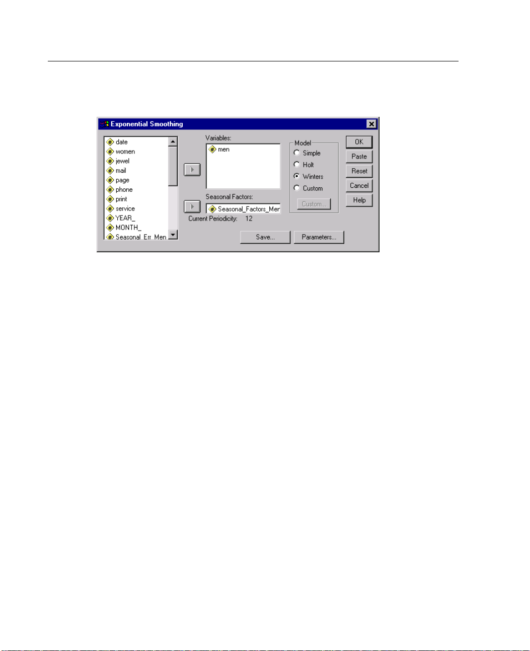
Figure 3-1
Exponential Smoothing dialog box
E Select o
ne or more variables from the available list and move them into the Variables
list. Note that the list includes only numeric variables.
E Select the type of model to use. These models differ in their trend and seasonal
components.
Simple. The simple model assumes that the series has no trend and no seasonal
variation.
Holt. The Holt model assumes that the series has a linear trend and no seasonal
on.
variati
s.
Winter
The Winters model assumes that the series has a linear trend and
multiplicative seasonal variation (its magnitude increases or decreases with the
overall level of the series). The Winters model is unavailable unless you have
defined
Custom
dates with the Define Dates dialog box, available from the Data menu.
.
A custom model allows you to specify the trend and seasonality
components.
For seas
onal models, the series must contain at least four full seasons of data.
The following options are also available:
For models with seasonal components, you can specify a set of seasonal factors or
allow T
rends to determine them for you.
Page 31
17
Click Save to specify how new variables are to be saved or to select options
for predict
Click Param
ing cases.
to set the parameter values for the model, or specify a grid
eters
search to determine the best-fitting parameter values.
Custom Exponential Smoothing Models
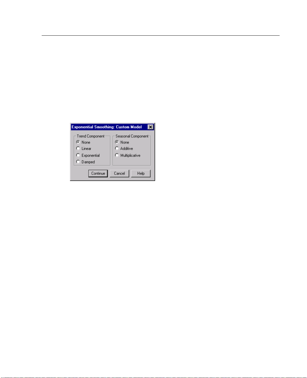
Figure 3-2
Exponential Smoothing Custom Model dialog box
Trend Component. Choices for the custom trend component include no trend, linear
trend, ex
None. Th
Linear.
Exponential. The mean level of the series increases or decreases exponentially
Damped. The mean level of the series increases or decreases with time, but the
ponential trend, and damped trend.
e level of the series does not show any overall linear trend.
The mean level of the series increases or decreases linearly (at a constant
rate) with time.
with time.
rate of c
hange declines. A trend that is dying out.
Exponential Sm
oothing
Seasonal Component. Choices for the custom seasonal component include no
seasonality, additive seasonality, and multiplicative seasonality.
None. Theseriesdoesnotshowperiodicvariation at the periodicity defined for it.
Additive. The series has seasonal variation that is additive: the magnitude of
seasonal variation does not depend on the overall level of the series.
Multiplicative. The series shows periodic variation at the periodicity defined for it,
and the s
ize of the periodic variation depends on the overall level of the series.
Page 32
18
Chapter 3
The Holt model in the main Exponential Smoothing dialog box is equivalent to
selecting Linear for Trend Component and None for Seasonal Component in the
Custom dial
Component and Multiplicative for Seasonal Component.
og box. The Winters model is equivalent to selecting
Linear for Trend
Exponentia
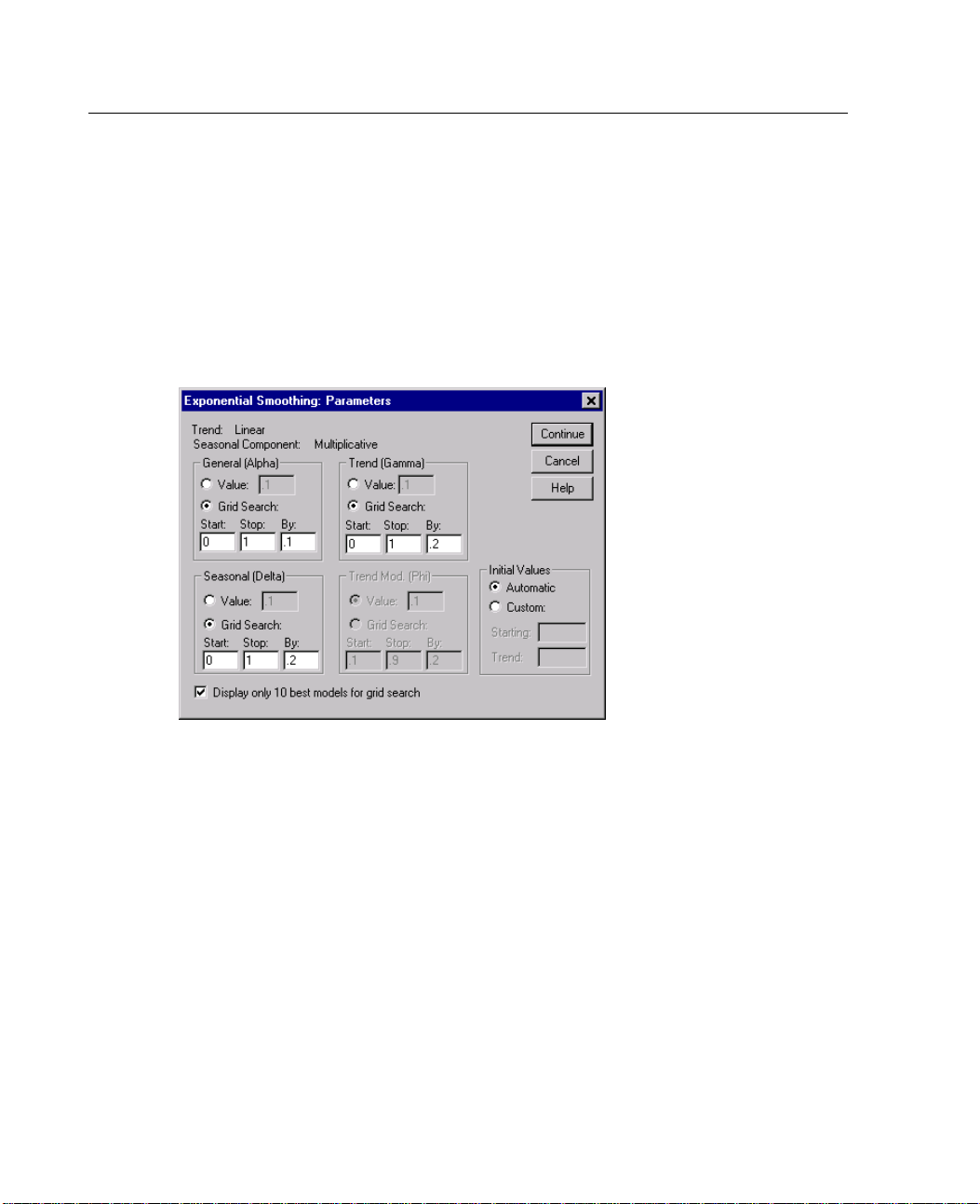
Figure 3-3
Exponential Smoothing Parameters dialog box
Alpha. Exponential smoothing parameter that controls the relative weight given to
recent observations, as opposed to the overall series mean. When alpha equals 1,
the single most recent observation is used exclusively; when alpha equals 0, old
observations count just as heavily as recent ones. Alpha is used for all models.
l Smoothing Parameters
Gamma. Exponential smoothing parameter that controls the relative weight given to
recent observations in estimating the present series trend. It ranges from 0 to 1,
with higher values giving more weight to recent values. Gamma is used only for
exponential smoothing models with a linear or exponential trend, or a damped trend
and no seasonal component. It is not used for the simple model.
Delta. Exponential smoothing parameter that controls the relative weight given to
recent observations in estimating the present seasonality. It ranges from 0 to 1, with
values near 1 giving higher weight to recent values. Delta is used for all exponential
Page 33

19
Exponential Sm
oothing
smoothing models with a seasonal component. It is not used for the simple or Holt
models.
Phi. Expone
ntial smoothing parameter that controls the rate at which a trend is
"damped," or reduced in magnitude over time. It ranges from 0 to 1 (but cannot
equal 1), with values near 1 representing more gradual damping. Phi is used for
exponentia
l smoothing models with a damped trend. It is not used for the simple,
Holt, or Winters models.
Value. Values for alpha, gamma and delta can be any value between and including 0
and 1. For p
Grid Search. The parameter is assigned a starting value in the Start box, an increment
hi, the value can be any value between but not including 0 and 1.
value in the By box, and an ending value in the Stop box. Enter these values after
selecting
Grid Search. The ending value must be greater than the starting value, and
the increment value must be less than their difference.
Initial Values. You can specify the starting and trend values used in smoothing the
series by
Automat
selecting one of the following:
ic.
The program calculates suitable starting and trend values from the
data. This is usually desirable.
Custom. Enter a number in the Start text box and, for models with a trend, a
number in the Trend text box. Poor choice of initial values can result in an
inferior
solution.
Display only 10 best models f or grid search. The parameter value(s) and sum of squared
errors (SSE) are displayed for only the 10 parameter combinations with the lowest
SSE rega
rdless of the number of parameter combinations tested. If this option is not
selected, all tested parameter combinations are displayed.
Page 34
20
Chapter 3
Saving Predi
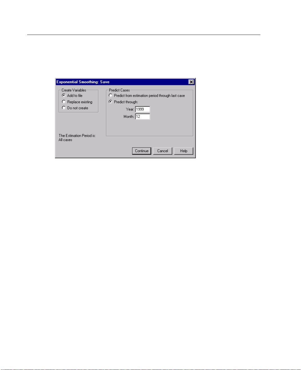
Figure 3-4
Exponential Smoothing Save dialog box
Create Variables. Allows you to choose how to treat new variables.
Addtofile. The new series are saved as regular variables in your working data
file. Variable names are formed from a three-letter prefix, an underscore, and a
number.
Replace existing. The new series are saved as temporary variables in the working
data file, and any existing temporary variables created by Trends commands
are dropped. Variable names are formed from a three-letter prefix, a pound
sign (#), and a number.
Do not create. Thenewseriesarenotaddedtotheworkingdatafile.
cted Values and Residuals
Predict Cases. Allows you to use the estimated model to predict values of the
dependent variable:
Predict from estimation period through last case. Predicts values for all cases from
the estimation period through the end of the file but does not create new cases. If
you are analyzing a range of cases that start after the beginning of the file, cases
prior to that range are not predicted. If no estimation period has been defined,
all cases are used to predict values.
Predict through. Predicts values through the specified date, time, or observation
number, based on the cases in the estimationperiod.Thiscanbeusedtoforecast
values beyond the last case in the time series. The text boxes that are available
Page 35

21
for specifying the end of the prediction period depend on the currently defined
date variab
les.
EXSMOOTH Command Additional Features
The SPSS command language also allows you to:
Specify initial seasonal factor estimates for seasonal models. Seasonal factors
can be specified numerically by providing as many additive or multiplicative
numbersast
See the SPSS Command Syntax Reference for complete syntax information.
he seasonal periodicity.
Exponential Sm
oothing
Page 36

Page 37

Chapter
4
Autoregress
The Autoregression procedure estimates true regression coefficients from time series
with first(Prais-Winsten and Cochrane-Orcutt) transform the regression equation to remove
the autocorrelation. The third (maximum likelihood) uses the same algorithm that
the ARIMA p
(ML) estimation is more demanding computationally but gives better results—and it
can tolerate missing data in the series.
Example.
per-capita income and the price level of the spirits in question for that year? A
standard regression analysis may not be valid in this case because the variables
represen
any two trending series will correlate simply because of the trends, regardless of
whether they are causally related or not. Autoregression allows you to remove the
autocor
relationships between dependent variables and candidate regressors.
order autocorrelated errors. It offers three algorithms. Two algorithms
rocedure uses for estimating autocorrelation. Maximum-likelihood
Is the consumption of alcoholic spirits in any given year related to real
t time series. Most time series have some trend, either up or down, and
relation inherent in many time series and ascertain any statistically significant
ion
Statistics. For the Prais-Winsten and Cochrane-Orcutt estimation methods: rho
value w
iteration; R, R
and regression statistics for the ordinary least-square and final Prais-Winsten or
Cochra
coefficients, adjusted sum of squares, and Marquardt constant at each iteration. For
the final maximum-likelihood parameter estimates: regression statistics, correlation
matri
residual variance, model standard error, log-likelihood, Akaike’s information
criterion, and Schwartz’s Bayesian criterion.
Metho
(equivalenttoanARIMA(1,0,0)model).
ith standard error, Dubin-Watson statistic, and mean squared error at each
2
,adjustedR2, standard error of the estimate, analysis-of-variance table,
ne-Orcutt estimates. For the maximum-likelihood method: rho, regression
x, covariance matrix, residual sum of squares, adjusted residual sum of squares,
ds.
Prais-Winsten, Cochrane-Orcutt, and Exact maximum-likelihood
23
Page 38
24
Chapter 4
Data. The dependent variable and any independent variables should be numeric.
Assumptions. Unless the maximum-likelihood method is used, the dependent variable
and any inde
pendent variables should not contain any embedded missing data. The
time series to be modeled should be stationary.
Stationary. A condition that must be met by the time series to which you fit an
ARIMA model
. Pure MA series will be stationary; however, AR and ARMA
series might not be. A stationary series has a constant mean and a constant
variance over time.
To C reate a
E From the m
Analyze
Time Series
Autoregression...
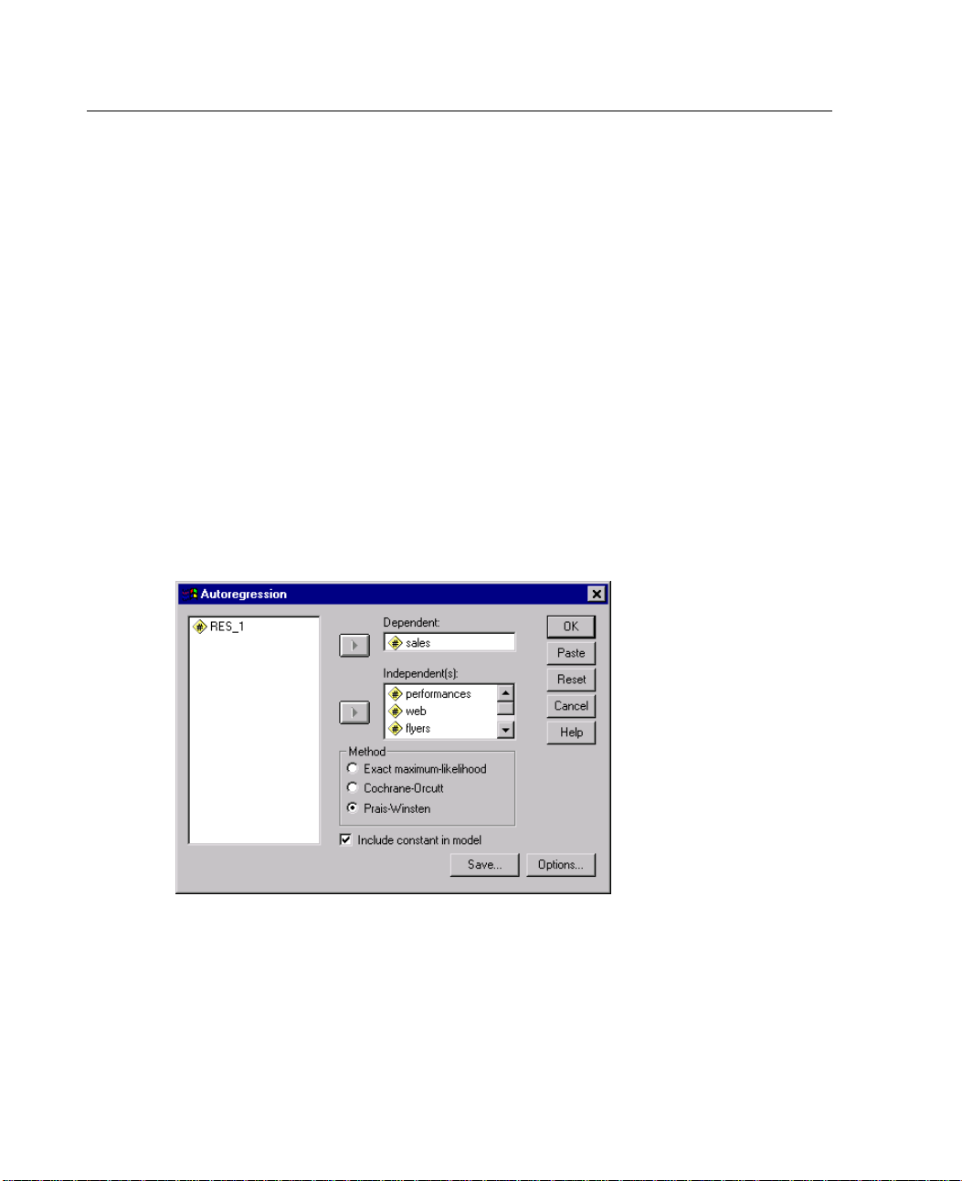
Figure 4-1
Autoregre
E Select a variable from the available list and move it into the Dependent list. Note that
n Autoregression Model
enus choose:
ssion dialog box
the list includes only numeric variables.
E Select one or more variables from the available list and move them into the
Independent(s) list.
Page 39
25
Autoregressio
E
Select one of the Method options to choose an estimation technique. Available
methods are Exact maximum-likelihood, Cochrane-Orcutt, and Prais-Winsten.
Exact maximum-likelihood. An estimation technique that for a given model and set
of data finds the parameter estimates that are "most likely" to have produced the
observed da
ta. This method can handle missing data within the series and can be
used when one of the independent variables is the lagged dependent variable.
Cochrane-Orcutt. A simple and widely used estimation procedure for estimating a
regression equation whose errors follow a first-order autoregressive process. It
cannot be u
Prais-Wi
sed when a series contains embedded missing values.
nsten.
A generalized least-squares method for estimating a regression
equation whose errors follow a first-order autoregressive process. It cannot
be used when a series contains embedded missing values. Generally, the
Prais-Win
sten method is preferable to the Cochrane-Orcutt method.
The following options are also available:
Deselect Include constant in model if you do not want to estimate a constant term.
Click Save to specify how new variables are to be saved or to select options
for predic
Click Opt
ting cases.
to select the initial value of the autoregressive parameter, set
ions
convergence criteria, or choose how to display parameters in the output.
n
Autoregression Options
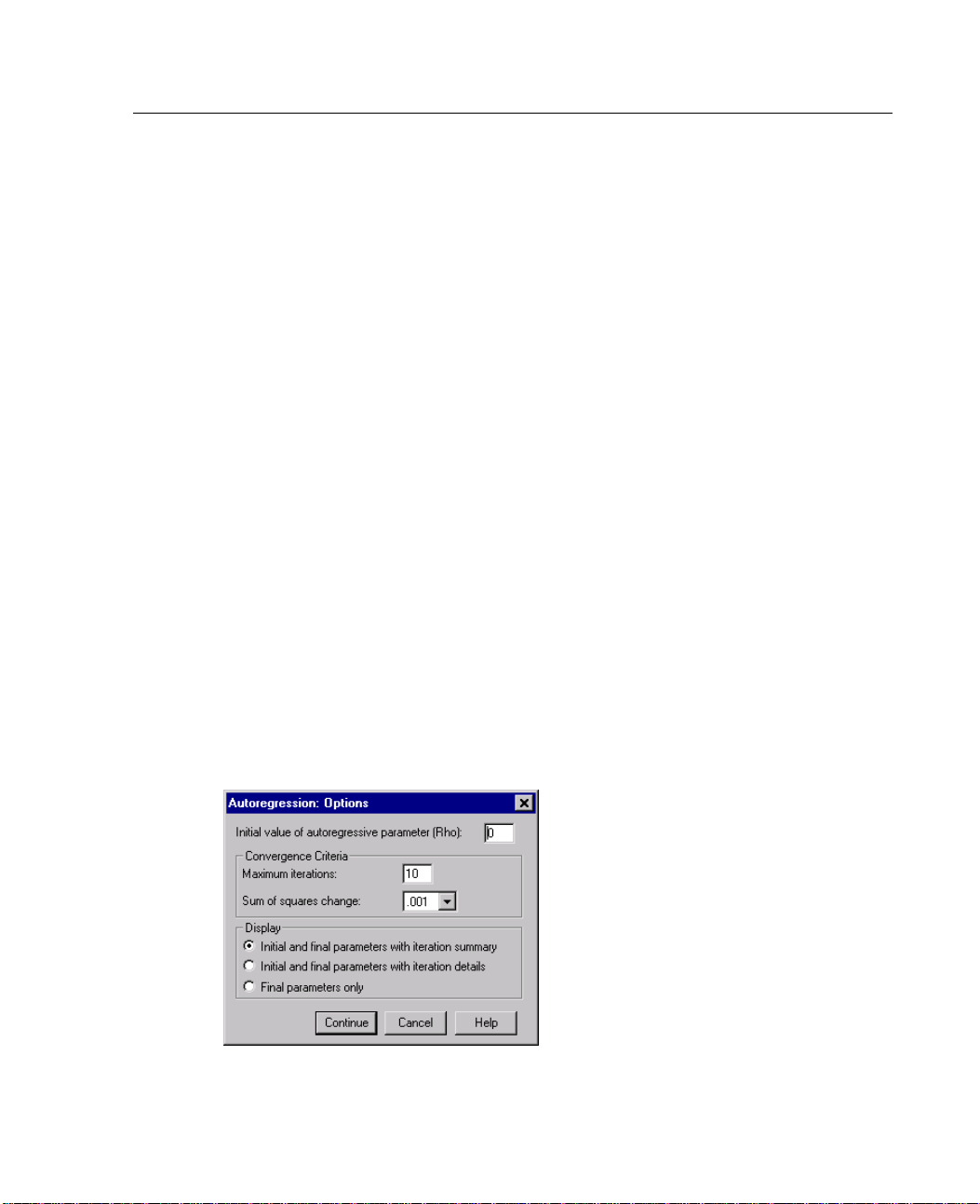
Figure 4-2
Autoregression Options dialog box
Page 40

26
Chapter 4
Initial value of autoregressive parameter. The value from which the iterative search for
the optimal value of rho begins. You can specify any number less than 1 and greater
than -1, alt
Convergence Criteria. Allowsyoutospecifythecriteriausedtodeterminewhen
hough negative values of rho are uncommon in this procedure.
iteration ceases.
Maximum iterations. The iterative algorithm stops after the number of specified
iterations even if the algorithm has not converged. You can specify a positive
integer in
Sum of squa
this text box.
res change.
The iterative algorithm stops if the adjusted sums of
squares does not decrease by 0.001% from one iteration to the next. You can
choose a smaller or larger value f or more or less precision in the parameter
estimates
. For greater precision, it may be necessary to increase the maximum
iterations.
Display. A
Initial a
llows you to control the information that is printed in the output.
nd final parameters with iteration summary.
Displays the initial and final
parameter estimates, goodness-of-fit statistics, the number of iterations, and
the reason that iteration terminated.
Initial and final parameters with iteration details. Displays the initial and final
paramete
r estimates, the parameter estimates after each iteration, goodness-of-fit
statistics, the number of iterations, and the reason that iteration terminated.
Final parameters only. Displays the final parameter estimates and goodness-of-fit
statistics.
Page 41
27
Saving Predi
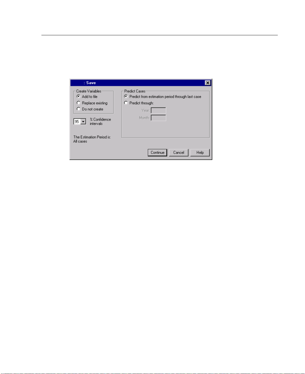
Figure 4-3
Save dialog box
Create Variables. Allows you to choose how to treat new variables.
Addtofile. The new series are saved as regular variables in your working data
file. Variable names are formed from a three-letter prefix, an underscore, and a
number.
Replace existing. The new series are saved as temporary variables in the working
data file, and any existing temporary variables created by Trends commands
are dropped. Variable names are formed from a three-letter prefix, a pound
sign (#), and a number.
Do not create. Thenewseriesarenotaddedtotheworkingdatafile.
cted Values and Residuals
Autoregressio
n
Confidence intervals. Displays confidence limits for the forecast. As long as the
process remains the same, you should expect N% of the series to remain between the
upper and lower confidence limits. Choose a level from the drop-down list.
Predict Cases. Allows you to use the estimated model to predict values of the
dependent variable.
Predict from estimation period through last case. Predicts values for all cases from
the estimation period through the end of the file but does not create new cases. If
you are analyzing a range of cases that start after the beginning of the file, cases
Page 42

28
Chapter 4
prior to that range are not predicted. If no estimation period has been defined,
all cases ar
Predict thr
eusedtopredictvalues.
ough.
Predicts values through the specified date, time, or observation
number, based on the cases in the estimationperiod.Thiscanbeusedtoforecast
values beyond the last case in the time series. The text boxes that are available
for specify
ing the end of the prediction period depend on the currently defined
date variables.
Autoregression Performance and Embedded Missing Data
When you request maximum-likelihood estimation with the Autoregression
procedure, Trends uses the same algorithms as in ARIMA. This means
that Autor
maximum-likelihood estimation is requested, but it may take a while.
To reduce processing time when your series has embedded missing data, you can
follow th
Options dialog box does not have controls for initial values, you need to use command
syntax to apply initial estimates the second time you run the Autoregression
procedu
procedure). The command is:
egression can process series with embedded missing data when
e same steps outlined for ARIMA. However, since the Autoregression
re (see step 3 of the process for improving the performance of the A RIMA
AREG /AP
Again, i
PLY INITIAL.
f processing time is not a consideration, you can simply use the
Autoregression procedure directly on the series with embedded missing data.
Alternatively, if you do not need the best-quality estimates, you can stop after
fying the model and estimating the coefficients for the series without missing
identi
data (see step 2 of the process for improving the performance of the ARIMA
procedure) and get results as good as you would with most other packages.
AREG Command Additional Features
The SPSS command language also allows you to:
Use the final estimate of rho from a previous execution of Autoregression as the
l estimate for iteration.
initia
Exerc
ise more precise control over convergence criteria.
Page 43

29
Autoregressio
See the SPSS Command Syntax Reference for complete syntax information.
n
Page 44

Page 45

ARIMA
This procedure estimates nonseasonal and seasonal univariate ARIMA
(Autoregre
models) with or without fixed regressor variables. The procedure produces
maximum-likelihood estimates and can process time series with missing observations.
Chapter
5
ssive Integrated Moving Average) models (also known as “Box-Jenkins”
Example. Y
to know if and when random fluctuations in product quality exceed their usual
acceptable levels. You’ve tried modeling product quality scores with an exponential
smoothin
data—that the model does little more than predict the overall mean and hence is of
little use. ARIMA models are well suited for describing complex time series. After
building
with the upper and lower confidence intervals produced by the model. Scores that fall
outside of the confidence intervals may indicate a true decline in product quality.
Statist
moving average), regression coefficients, adjusted sum of squares, and Marquardt
constant. For the final maximum-likelihood parameter estimates: residual sum of
square
log-likelihood, Akaike’s information criterion, Schwartz’s Bayesian criterion,
regression statistics, correlation matrix, and covariance matrix.
Data. T
Assumptions. The time series to be modeled should be stationary.
Stationary. A condition that must be met by the time series to which you fit an
ou are in charge of quality control at a manufacturing plant and need
g model but found—presumably because of the highly erratic nature of the
an appropriate ARIMA model, you can plot the product quality scores along
ics.
For each iteration: seasonal and nonseasonal lags (autoregressive and
s, adjusted residual sum of squares, residual variance, model standard error,
he dependent variable and any independent variables should be numeric.
ARIMA m
series might not be. A stationary series has a constant mean and a constant
variance over time.
odel. Pure MA series will be stationary; however, AR and ARMA
31
Page 46
32
Chapter 5
Obtaining an ARIMA Analysis
E From the menus choose:
Analyze
Time Series
ARIMA
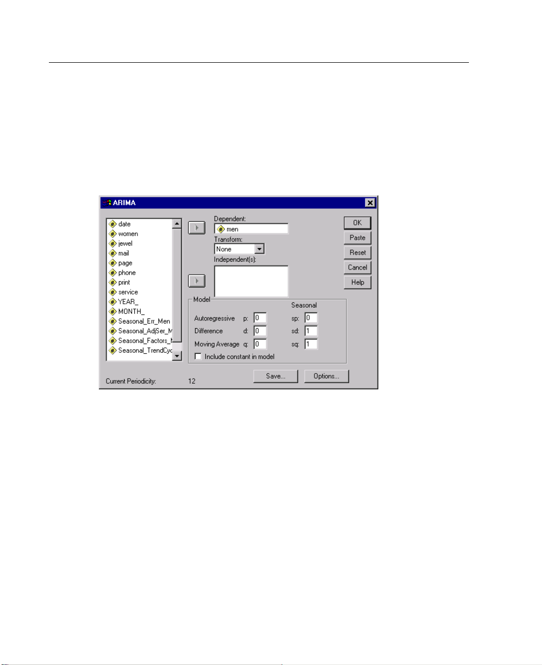
Figure 5-1
ARIMA dialog box
E Select one variable from the available list a nd move it into the Dependent list. Note
that the list includes only numeric variables.
E Specify values for the parameters of the ARIMA model: Autoregressive, Difference,
and Movi
ng Average. These parameters are commonly referred to as p, d, and q,
respectively.
Autoregressive. The number of autoregressive parameters in the model. Specify a
gative integer. Each parameter measures the independent effect of values
non-ne
with a specified lag. Thus, an autoregressive order of 2 means that a series value
is affected by the preceding two values (independently of one another).
Page 47

ARIMA
Difference. d is the number of times the series must be differenced to make
it stationa
ry. Specify a non-negative integer. Enter 0 if the process is already
stationary.
Moving Average. q is the order of moving average of the process. Specify a
non-negative integer. Enter 0 for an autoregressive process, 1 for a first-order
moving aver
Transform. To analyze the dependent variable in a logarithmic scale, select one of
age, 2 for a second-order moving average, etc.
the alternatives o n the drop-down list. If you select a log transformation, ARIMA
transform
s the predicted values (fit) and confidence intervals (lcl and ucl) that it
creates back into the original metric but leaves the residuals (err) in the log metric
for diagnostic purposes.
33
Seasonal.
The seasonal column contains text boxes in which you can specify the
corresponding parameters (sp, sd, and sq) of the process at seasonal lags. These
values can be 0 or a positive integer, usually 1. The Seasonal boxes are unavailable if
no period
icity is defined. The current periodicity is displayed at the bottom of the
dialog box.
Optionally, you can:
Select one or more independent variables and move them into the Independent(s)
list. Note that the list includes only numeric variables.
Deselect Include constant in model if you do not want to estimate a constant term.
Click Save to specify how new variables are to be saved or to select options
for predi
Click Op
cting cases.
to select convergence criteria, set initial values for the model, select
tions
the forecasting method, or choose how to display parameters in the output.
Page 48
34
Chapter 5
ARIMA Option
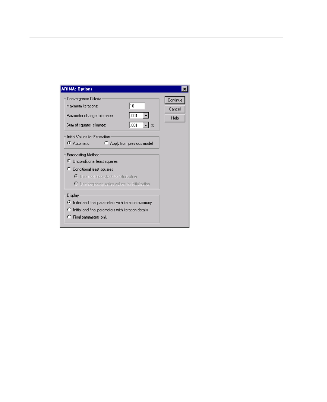
Figure 5-2
ARIMA Options dialog box
Convergence Criteria. Allowsyoutospecifythecriteriausedtodeterminewhen
iteration ceases.
Maximum iterations. The iterative algorithm stops after the number of specified
iterations even if the algorithm has not converged. You can specify a positive
integer in this text box.
Parameter change tolerance. Iteration stops if no parameter changes by more than
0.001 from one iteration to the next. You can choose a smaller or larger value for
more or less precision in the parameter estimates. For greater precision, it may
also be necessary to increase the maximum iterations.
Sum of squares change. The iterative algorithm stops if the adjusted sums of
squares does not decrease by 0.001% from one iteration to the next. You can
choose a smaller or larger value f or more or less precision in the parameter
estimates. For greater precision, it may be necessary to increase the maximum
iterations.
s
Page 49

ARIMA
Initial Values for Estimation. Allows you to select how initial values for the model are
determined.
Automatic. ARIMA chooses initial values.
Apply from previous model. The parameter estimates from the previous execution
of ARIMA (in the same session) are used as initial estimates. This can save time
if the data a
Forecasting Method. Allows you to specify the forecasting method to use.
Unconditional least squares. The forecasts are unconditional least squares
forecasts.
Condition
nd model are similar to the last one used.
They are also called finite memory forecasts.
al least squares.
The forecasts are conditional least squares forecasts.
They are also called infinite memory forecasts
Use model constant for initialization. The forecasts are computed by assuming
that the unobserved past errors are 0 and that the unobserved past values of the
response s
Use begin
eries are equal to the mean.
ning series values for initialization.
The beginning series values are used
to initialize the recursive conditional least squares forecasting algorithm.
35
Display. A
Initial a
llows you to control the information that is printed in the output.
nd final parameters with iteration summary.
Displays the initial and final
parameter estimates, goodness-of-fit statistics, the number of iterations, and
the reason that iteration terminated.
Initial and final parameters with iteration details. Displays the initial and final
parameter
estimates, the parameter estimates after each iteration, goodness-of-fit
statistics, the number of iterations, and the reason that iteration terminated.
Final parameters only. Displays the final parameter estimates and goodness-of-fit
statistics.
Page 50
36
Chapter 5
Saving Predi
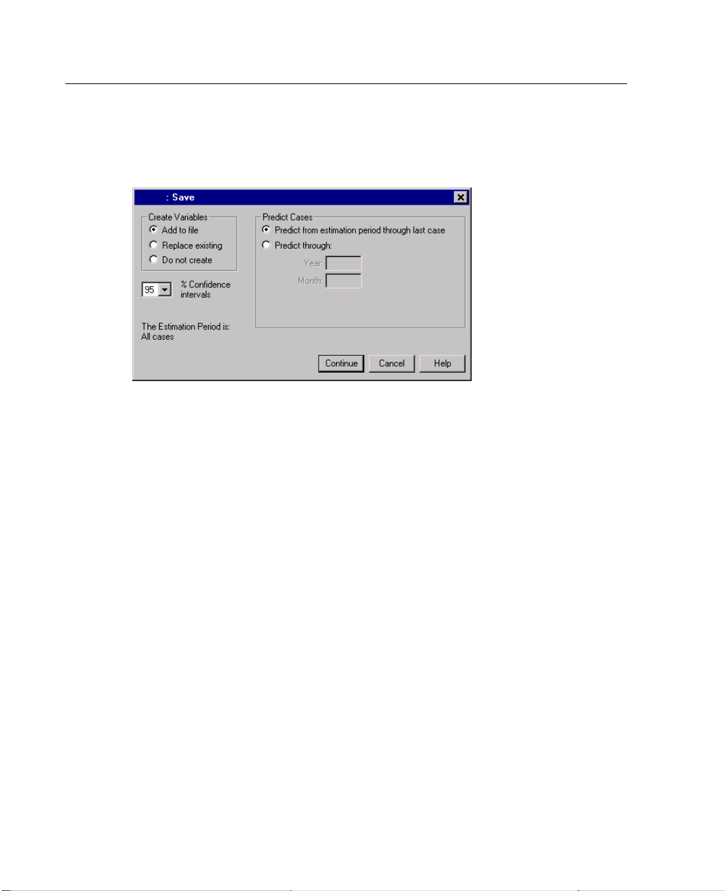
Figure 5-3
Save dialog box
Create Variables. Allows you to choose how to treat new variables.
Addtofile. The new series are saved as regular variables in your working data
file. Variable names are formed from a three-letter prefix, an underscore, and a
number.
Replace existing. The new series are saved as temporary variables in the working
data file, and any existing temporary variables created by Trends commands
are dropped. Variable names are formed from a three-letter prefix, a pound
sign (#), and a number.
Do not create. Thenewseriesarenotaddedtotheworkingdatafile.
cted Values and Residuals
Confidence intervals. Displays confidence limits for the forecast. As long as the
process remains the same, you should expect N% of the series to remain between the
upper and lower confidence limits. Choose a level from the drop-down list.
Predict Cases. Allows you to use the estimated model to predict values of the
dependent variable.
Predict from estimation period through last case. Predicts values for all cases from
the estimation period through the end of the file but does not create new cases. If
you are analyzing a range of cases that start after the beginning of the file, cases
Page 51

prior to that range are not predicted. If no estimation period has been defined,
all cases ar
Predict thr
eusedtopredictvalues.
ough.
Predicts values through the specified date, time, or observation
number, based on the cases in the estimationperiod.Thiscanbeusedtoforecast
values beyond the last case in the time series. The text boxes that are available
for specify
ing the end of the prediction period depend on the currently defined
date variables.
ARIMA Performance and Embedded Missing Data
In the presence of embedded missing data, the SPSS Trends ARIMA procedure uses
a technique called Kalman filtering, which requires considerably more calculation
than the si
a single embedded missing value increases ARIMA processing time greatly—in
extreme cases, by a factor of 10.
If you wan
can use the following procedure to reduce processing time:
1. Make a copy of the series with valid data interpolated in place of the embedded
missing data.
mpler technique used when no embedded missing data are present. Even
t to use ARIMA on a series that contains embedded missing data, you
37
ARIMA
2. Identify the correct model and estimate the coefficients for the series without missing
data. AR
IMA can use a much faster algorithm when no embedded missing data
are present.
3. Once you have found the correct model, run ARIMA on the original series to get
the best possible estimates for the coefficients, using Kalman filtering to handle the
missing
previous model
data. This time, open the ARIMA Options dialog box and select
for Initial Values for Estimation. This should reduce the number
Apply from
of iterations needed this time.
Most ARIMA packages allow only the first two steps. You can always stop there
with Tr
ends ARIMA too, but you have the option of using the Kalman filtering
algorithm to get the best possible estimates.
Page 52

38
Chapter 5
Note that the results obtained by following the steps above are the same as the
results you would obtain if you used the ARIMA procedure directly on the series with
embedded mi
The only difference is processing time.
ssing data, without first estimating initial values from interpolated data.
ARIMA Comma
The SPSS co
Specify co
parameters (either regular or s easonal) are estimated only for specified orders.
Exercise more precise control over convergence criteria.
See the SPS
nd Additional Features
mmand language also allows you to:
nstrained models in which autoregressive or moving average
S Command Syntax Reference for complete syntax information.
Page 53

Chapter
6
Seasonal Dec
The Seasonal Decomposition procedure decomposes a series into a seasonal
component, a combined trend and cycle component, and an “error” component. The
procedure is an implementation of the Census Method I, otherwise known as the
ratio-to-moving-average method.
Example. A scientist is interested in analyzing monthly measurements of the ozone
level at a particular weather station. The goal is to determine if there is any trend in
the data. In order to uncover any real trend, the scientist first needs to account for the
variation in readings due to seasonal effects. The Seasonal Decomposition procedure
can be used to remove any systematic seasonal variations. The trend analysis is then
performed on a seasonally adjusted series.
Statistics. The set of seasonal factors.
Data. The variables should be numeric.
Assumptions. The variables should not contain any embedded missing data. At least
one periodic date component must be defined.
omposition
Estimating Seasonal Factors
E From the menus choose:
Analyze
Time Series
Seasonal Decomposition...
39
Page 54
40
Chapter 6
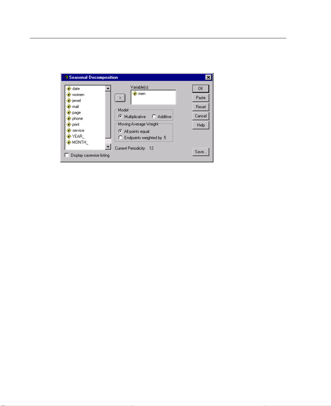
Figure 6-1
Seasonal Decomposition dialog box
E Selectone or more variables from the available list and move them into the Variable(s)
list. Note that the list includes only numeric variables.
Model. The Seasonal Decomposition procedure offers two different approaches for
modeling the seasonal factors: multiplicative or additive.
Multiplicative. The seasonal component is a factor by which the seasonally
adjusted series is multiplied to yield the original series. In effect, Trends
estimates seasonal components that are proportional to the overall level of the
series. Observations without seasonal variation have a seasonal component of 1.
Additive. The seasonal adjustments are added to the seasonally adjusted series
to obtain the observed values. This adjustment attempts to remove the seasonal
effect from a series in order to look at other characteristics of interest that may
be "masked" by the seasonal component. In effect, Trends estimates seasonal
components that do not depend on the overall level of the series. Observations
without seasonal variation have a seasonal component of 0.
Moving Average Weight. The Moving Average Weight options allow you to specify
how to treat the series when computing moving averages. These options are available
only if the periodicity of the series is even. If the periodicity is odd, all points are
weighted equally.
Page 55
41
All points equal. Moving averages are calculated with a span equal to the
periodicit
the periodicity is odd.
Endpoints weighted by .5. Moving averages for series with even periodicity are
calculated with a span equal to the periodicity plus 1 and with the endpoints
of the span w
Optionally, you can:
Click Save to specify how new variables should be saved.
Seasonal De
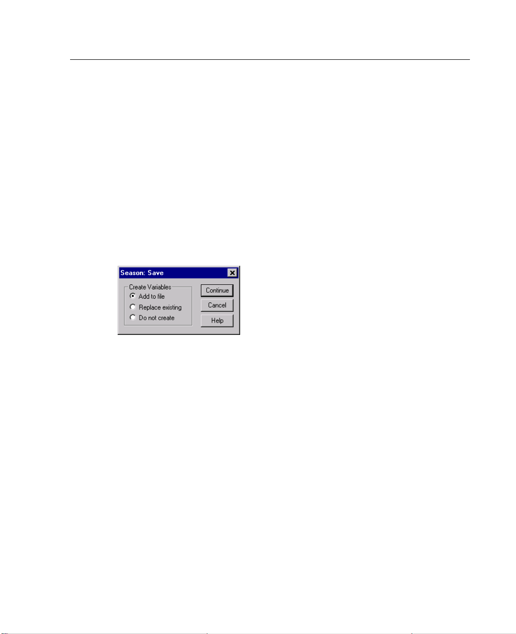
Figure 6-2
SeasonSavedialogbox
Seasonal Decom
y and with all points weighted equally. This method is always used if
eightedby0.5.
composition Save
position
Create Variables. Allows you to choose how to treat new variables.
Add to file. The new series created by Seasonal Decomposition are saved as
regular variables in your working datafile.Variablenamesareformedfroma
three-letter prefix, an underscore, and a number.
Replace existing. The new series created by Seasonal Decomposition are saved as
temporary variables in your working data file. At the same time, any existing
temporary variables created by the Trends procedures are dropped. Variable
names are formed from a three-letter prefix, a pound sign (#), and a number.
Do not create. Thenewseriesarenotaddedtotheworkingdatafile.
SEASON Command Additional F eatures
The SPSS command language also allows you to:
Specify any periodicity within the SEASON command rather than select one of the
alternatives offered by the Define Dates procedure.
Page 56

42
Chapter 6
See the SPSS Command Syntax Reference for complete syntax information.
Page 57

Chapter
7
Spectral Plo
The Spectral Plots procedure is used to identify periodic behavior in time series.
Instead of analyzing the variation from one time point to the next, it analyzes the
variation of the series as a whole into periodic components of different frequencies.
Smooth series have stronger periodic components at low frequencies; random
variation (“white noise”) spreads the component strength over all frequencies.
Series that include missing data cannot be analyzed with this procedure.
Example. The rate at which new houses are constructed is an important barometer of
the state of the economy. Data for housing starts t ypically exhibit a strong seasonal
component. But are there longer cycles present in the data that analysts need to be
aware of when evaluating current figures?
Statistics. Sine and cosine transforms, periodogram value, and spectral density
estimate for each frequency or period component. When bivariate analysis is selected:
real and imaginary parts of cross-periodogram, cospectral density, quadrature
spectrum, gain, squared coherency, and phase spectrum for each frequency or period
component.
ts
Plots. For univariate and bivariate analyses: periodogram and spectral density.
For bivariate analyses: squared coherency, quadrature spectrum, cross amplitude,
cospectral density, phase spectrum, and gain.
Data. The variables should be numeric.
43
Page 58
44
Chapter 7
Assumptions. The variables should not contain any embedded missing data. The
timeseriestobeanalyzedshouldbestationaryandanynon-zeromeanshouldbe
subtracted
Stationar
out from the series.
y.
A condition that must be met by the time series to which you fit an
ARIMA model. Pure MA series will be stationary; however, AR and ARMA
series might not be. A stationary series has a constant mean and a constant
variance o
ver time.
Obtaining a Spectral Analysis
E From the menus choose:
Graphs
Time Serie
Spectral.
Figure 7-1
Spectral Plots dialog box
s
..
E Selec
t one or more variables from the available list and move them to the Variable(s)
list. Note that the list includes only numeric variables.
E Select one of the Spectral Windo w options to choose how to smooth the periodogram
in order t o obtain a spectral density estimate. Available smoothing options are
-Hamming, Tukey, Parzen, Bartlett, Daniell (Unit), and None.
Tukey
Page 59

45
Spectral Plots
Tukey-Hamming. The weights are Wk = .54Dp(2 pi fk) + .23Dp (2 pi fk + pi/p) +
.23Dp (2 pi f
k - pi/p), for k = 0, ..., p, where p is the integer part of half the span
and Dp is the Dirichlet kernel of order p.
Tukey. The weights are Wk = 0.5Dp(2 pi fk) + 0.25Dp (2 pi fk + pi/p) + 0.25Dp(2
pi fk - pi/p), for k = 0, ..., p, where p is the integer part of half the span and
Dp is the Dir
Parzen. Th
ichlet kernel of order p.
e weights are Wk = 1/p(2 + cos(2 pi fk)) (F[p/2] (2 pi fk))**2, for k= 0,
... p, where p is the integer part of half the span and F[p/2] is the Fejer kernel
of order p/2.
Bartlett. The shape of a spectral window for which the weights of the upper half
of the wind
ow are computed as Wk = Fp (2*pi*fk), for k = 0, ... p, where p is
the integer part of half the span and Fp is the Fejer kernel of order p. The lower
half is symmetric with the upper half.
Daniell (Unit). The shape of a spectral window for which the weights are all
equal to 1
None. No s
.
moothing. If this option is chosen, the spectral density estimate is
the same as the periodogram.
Bivariat
e analysis – first variable with each.
If you have selected two or more variables,
you can select this option to request bivariate spectral analyses.
The first variable in the Variable(s) list is treated as the independent variable, and
all remai
Each ser
ning variables are treated as dependent variables.
ies after the first is analyzed with the first series independently of other
series named. Univariate analyses of each series are also performed.
Span. The
range of consecutive values across which the smoothing is carried out.
Generally, an odd integer is used. Larger spans smooth the spectral density plot
more than smaller spans.
Center v
ariables.
Adjusts the series to have a mean of 0 before calculating the
spectrum and to remove the large term that may be associated with the series mean.
Plot. Periodogram and spectral density are available for both univariate and bivariate
analyse
Period
s. All other choices are available only for bivariate analyses.
ogram.
Unsmoothed plot of spectral amplitude (plotted on a logarithmic
scale) against either frequency or period. Low-frequency variation characterizes
a smooth series. Variation spread evenly across all frequencies indicates "white
"
noise.
Page 60

46
Chapter 7
Spectral density. A periodogram that has been smoothed to remove irregular
variation.
Cospectral
density.
The real part of the cross-periodogram, which is a measure of
the correlation of the in-phase frequency components of two time series.
Quadrature spectrum. The imaginary part of the cross-periodogram, which is a
measure of the correlation of the out-of-phase frequency components of two time
series. The
Cross ampl
components are out of phase by pi/2 radians.
itude.
The square root of the sum of the squared cospectral density
and the squared quadrature spectrum.
Gain. The quotient of dividing the cross amplitude by the spectral density for one
of the series. Each of the two series has its own gain value.
Squared coherency. Theproductofthegainsofthetwoseries.
Phase spectrum. A measure of the extent to which each frequency component
of one seri
By frequency. All plots are produced by frequency, ranging from frequency 0 (the
es leads or lags the other.
constant or mean term) to frequency 0.5 (the term for a cycle of two observations).
By period.
All plots are produced by period, ranging from 2 (the term for a cycle of
two observations) to a period equal to the number of observations (the constant or
mean term). Period is displayed on a logarithmic scale.
SPECTRA Command Additional Features
The SPSS command language also allows you to:
Save computed spectral analysis variables to the working data file for later use.
Specify custom weights for the spectral window.
Produce plots by both frequency and period.
Print a complete listing of each value shown in the plot.
See the SPSS Command Syntax Reference for complete syntax information.
Page 61
Part 2: Examples
Page 62

Page 63

Chapter
8
Exponential
Smoothing
Using Exponential Smoothing to Predict Future Sales
A catalog company is interested in forecasting monthly sales of its men’s clothing
s end, the company collected monthly sales of men’s clothing for a
onential Smoothing procedure to predict monthly sales of men’s
ples that follow, it is more convenient to use variable names rather than
Prelimina
E From the menus choose:
line. To thi
10-year period. This information is collected in catalog_seasfac.sav, found in the
\tutorial\sample_files\ subdirectory of the directory in which you installed SPSS.
Use the Exp
clothing for the following year.
ries
In the exam
variable labels.
Edit
Options...
49
Page 64
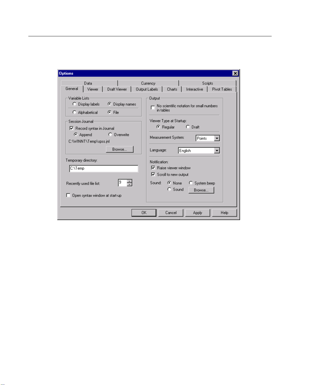
50
Chapter 8
Figure 8-1
Options dialog box
Unders
E Select Display names in the Variable Lists group.
E Click OK.
tanding Your Data
st step in analyzing a time series is to plot it. Visual inspection of a time series
The fir
can often be a powerful guide in choosing an appropriate exponential smoothing
model. In particular:
Does the series have an overall trend? Does the trend appear constant or does
it appear to be dying out with time?
Does the series show seasonality? Do the seasonal fluctuations seem to grow with
r do they appear constant over successive periods?
time o
Page 65
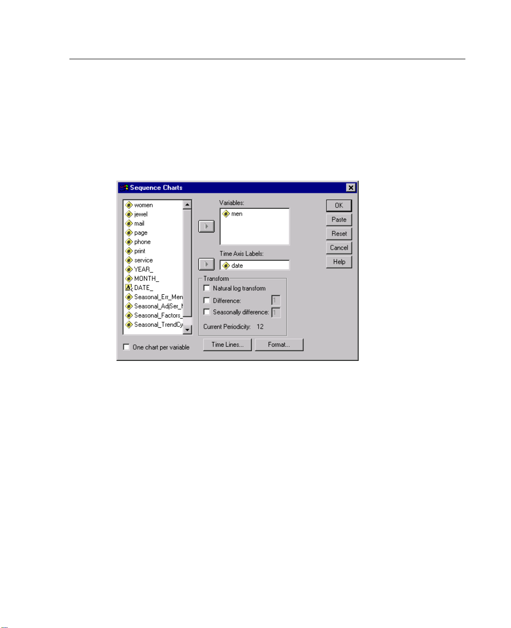
51
To obtain a plot of men’s clothing sales over time:
E From the menus choose:
Graphs
Sequence...
Figure 8-2
Sequence Charts dialog box
Exponential Sm
oothing
E Select
E Select
E Click T
men and move it into the Variables list.
date and move it into the Time Axis Labels list.
ime Lines
.
Page 66
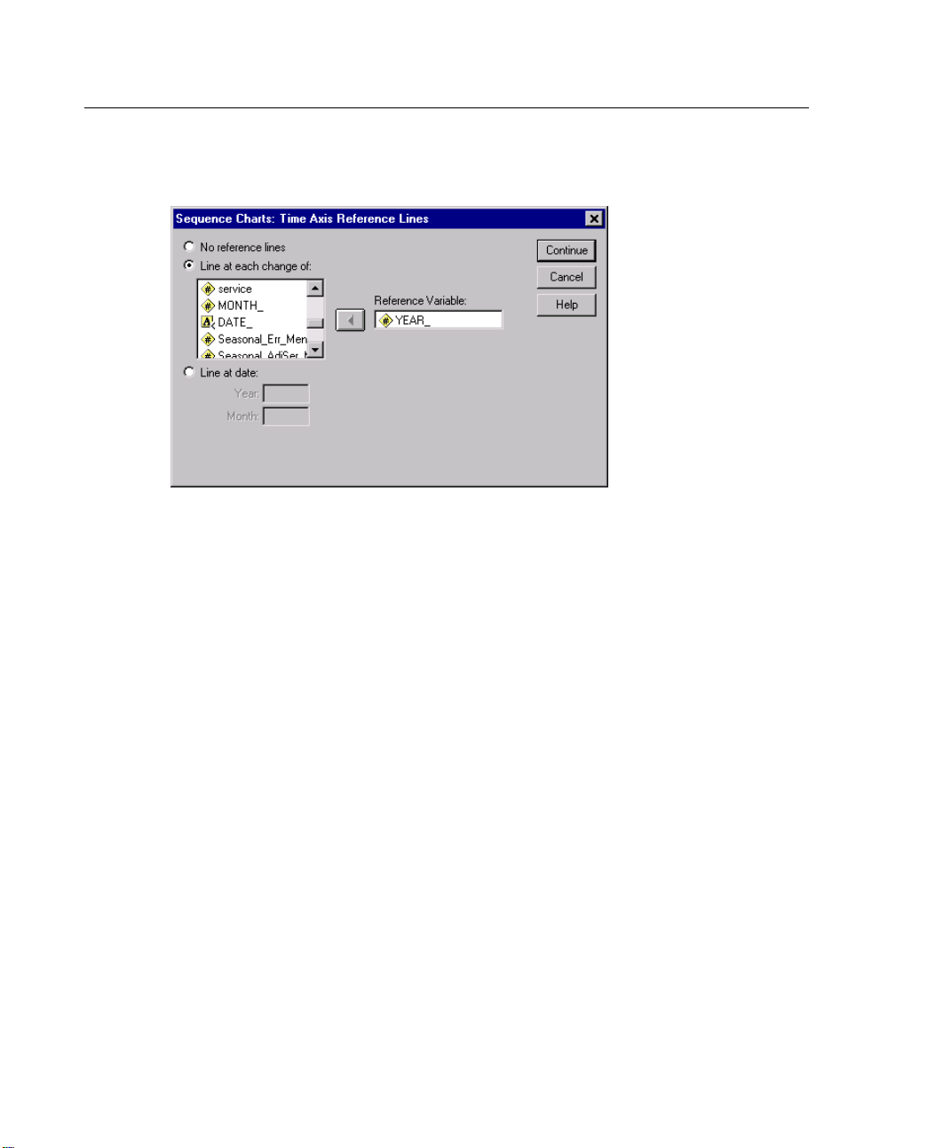
52
Chapter 8
Figure 8-3
Sequence Charts Time Axis Reference Lines dialog box
E Select Line at each change of.
E Select YEAR_ and move it into the Reference Variable list.
These cho
ices result in a vertical reference line at the start of each year, which is
useful for identifying annual seasonality.
E Click Continue.
E Click OK in the Sequence Charts dialog box.
Page 67
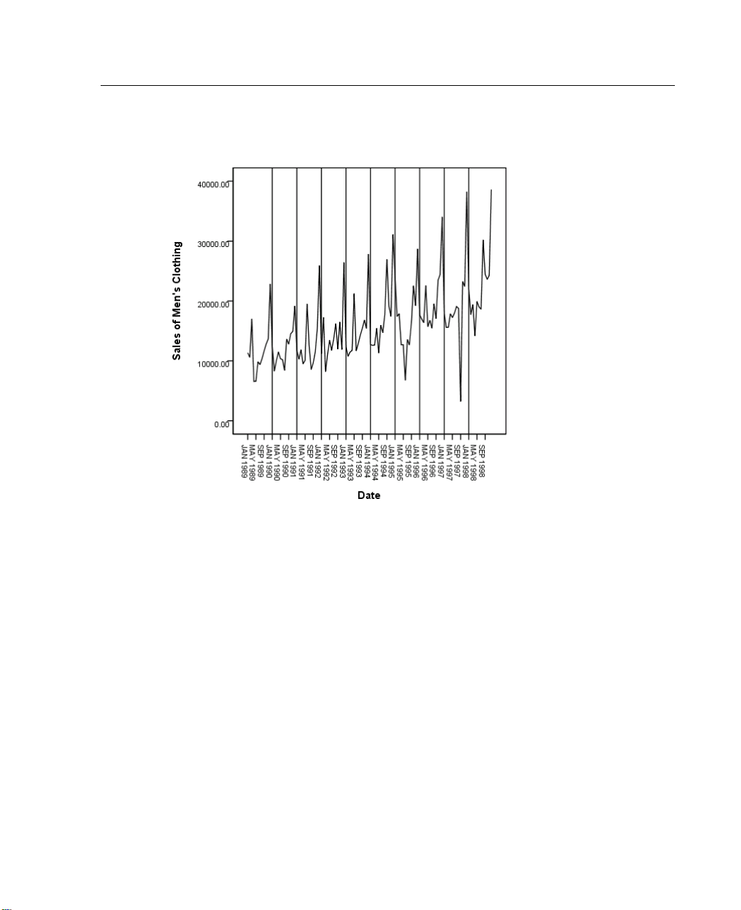
53
Figure 8-4
Sales of men’s clothing (in U.S. dollars)
Exponential Sm
oothing
The ser
ies shows a global upward trend; that is, the series values tend to increase over
time. The upward trend is seemingly constant, which indicates a linear trend.
The series also has a distinct seasonal pattern with annual highs in December. This
is easy
to see because of the vertical reference lines positioned at the start of each
year. The seasonal variations appear to grow with the upward series trend, which
suggests multiplicative rather than additive seasonality.
Building and Analyzing Exponential Smoothing Models
Building a best-fit exponential smoothing model involves determining the model
type—does the model need to include trend and/or seasonality—and then obtaining
st-fit parameters for the chosen model.
the be
Page 68
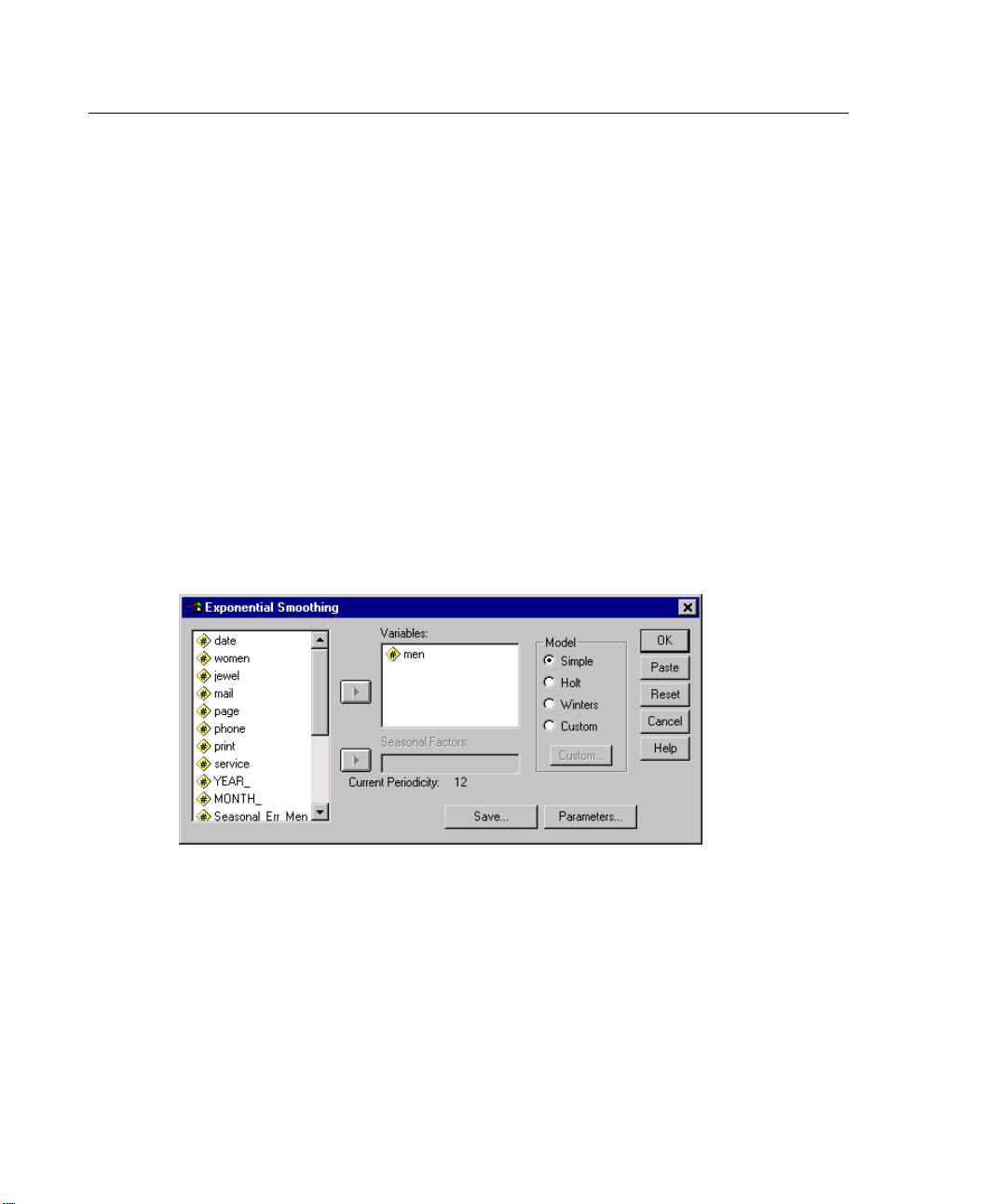
54
Chapter 8
The plot of men’s clothing sales over time suggested a model with both a linear
trend component and a multiplicative seasonality component. This implies a Winters
model. Firs
t, however, we will explore a simple model (no trend and no seasonality)
and then a Holt model (incorporates linear trend but no seasonality). This will give
you practice in identifying when a model is not a good fit to the data, which is an
essential
skill in successful model building.
Building and Analyzing a Simple Model
To build an exponential smoothing model:
E From the menus choose:
Analyze
Time Series
Exponential Smoothing...
Figure 8-5
Exponential Smoothing dialog box
E Select
E Select
E Click Pa
men and move it into the Variables list.
Simple in the Model group.
rameters
.
Page 69
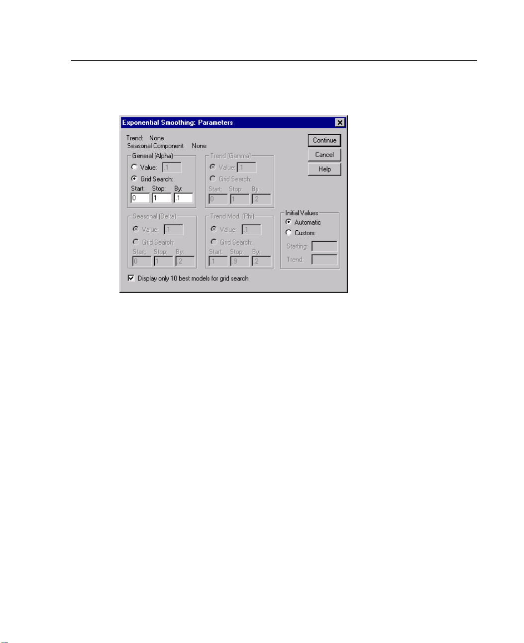
55
Exponential Sm
Figure 8-6
Exponential Smoothing Parameters dialog box
E Select Grid Search in the General (Alpha) group. Leave the Start, Stop, and By text
boxes wi
The
th their default values of 0, 1, and 0.1, respectively.
Grid Search option provides a convenient method for determining the best-fit
oothing
model parameters by calculating goodness-of-fit measures for each of the grid values.
The curr
ent selections result in values of alpha ranging from 0 to 1 in increments of
0.1.
Leave the default choice for displaying only the 10 best-fit models. The analysis is
rformed for each of the points in the grid, but the output is limited to displaying
still pe
results for the 10 best models.
E Click Continue.
E Click OK in the Exponential Smoothing dialog box.
Page 70
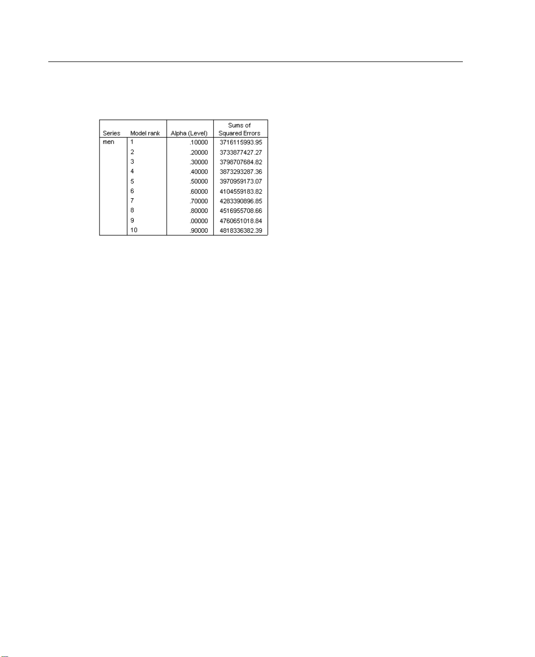
56
Chapter 8
Figure 8-7
Exponential smoothing , no trend or seasonality
The model output lists the 10 best-fitting values of alpha, along with the associated
sums of squared errors (SSE) for each value. Each value of alpha corresponds to a
different model, with models ranked according to their SSE value. A lower rank
implies a smaller SSE and thus a model that gives a better fit to the data. The SSE
measure of error is lowest when alpha is 0.1, indicating that an alpha of 0.1 gives
the best fit to the data for this class of models. This low value of alpha indicates that
the overall level of the series is best predicted when all observations have roughly
equal weight.
To see how well the simple model fits the data, you’ll need to reopen the Sequence
Charts dialog box. A convenient shortcut for reopening previous dialog boxes is as
follows:
E Click the Dialog Recall toolbar icon.
E Select the entry for the desired dialog box, which in this case is Sequence Charts.
Page 71
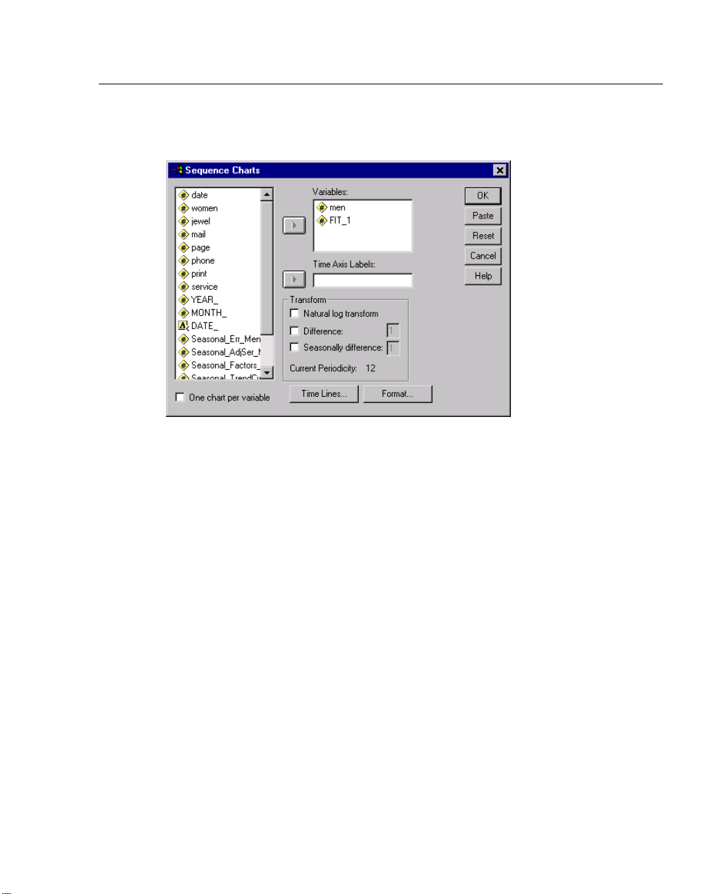
57
Figure 8-8
Sequence Charts dialog box
. This will restore the dialog box to its default settings, thus removing
E Click R
eset
the timeline settings used previously.
E Select men and FIT_1 and move them into the Variables list.
Exponential Sm
oothing
E Click OK.
Page 72
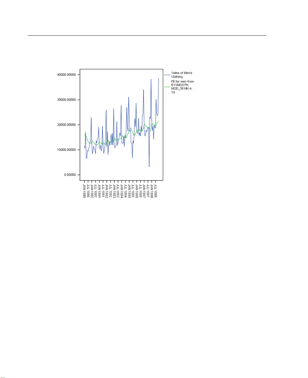
58
Chapter 8
Figure 8-9
Predictions from exponential smoothing, no trend or seasonality
Notice that the model, as expected, does not account for the observed seasonality. In
addition, it predicts an initial downward trend in contrast to the data, which exhibits a
continuing upward trend.
Examining the autocorrelations and partial autocorrelations for the residuals of the
best-fit simple model provides more quantitative insight than viewing the sequence
charts. Significant structure in either of these correlation functions would imply
that the underlying model is incomplete.
E From the menus choose:
Graphs
Time Series
Autocorrelations...
Page 73
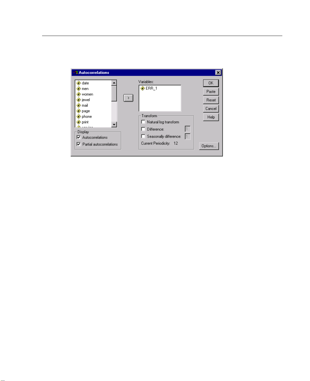
59
Exponential Sm
Figure 8-10
Autocorrelations dialog box
E Select the error variable ERR_1 associated with the fit from the simple model.
E Click OK.
oothing
Page 74
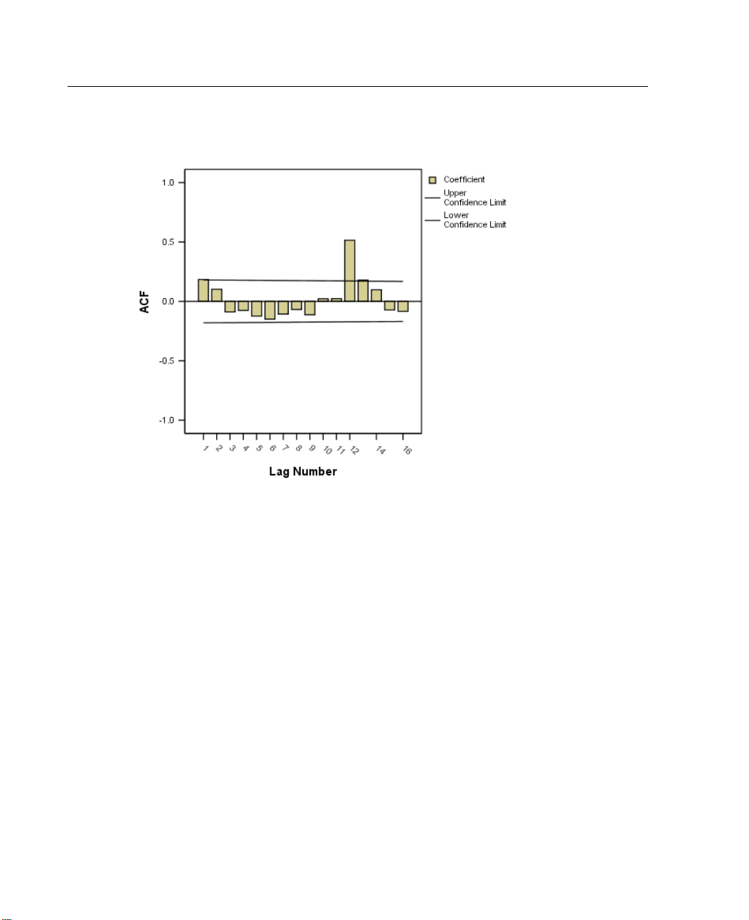
60
Chapter 8
Figure 8-11
Residual autocorrelation plot for simple model
The autocorrelation function shows a significant peak at a lag of 12. This is no
surprise, since the simple model doesn’t account for seasonality and there is a strong
annual seasonal component in the data.
Page 75
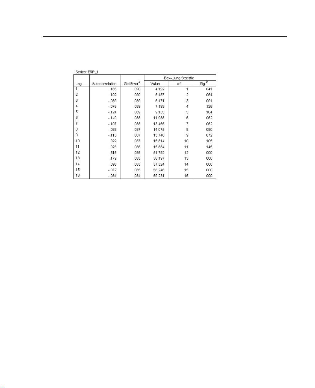
61
Exponential Sm
Figure 8-12
Residual autocorrelation statistics for simple model
oothing
Notice also that the Box-Ljung statistic at a lag of 12 is statistically significant. In
eassociatedp value is 0 to the stated precision. This underscores the fact that
fact, th
the lag 12 autocorrelation is significant and represents structure not accounted for
in the present model.
Page 76
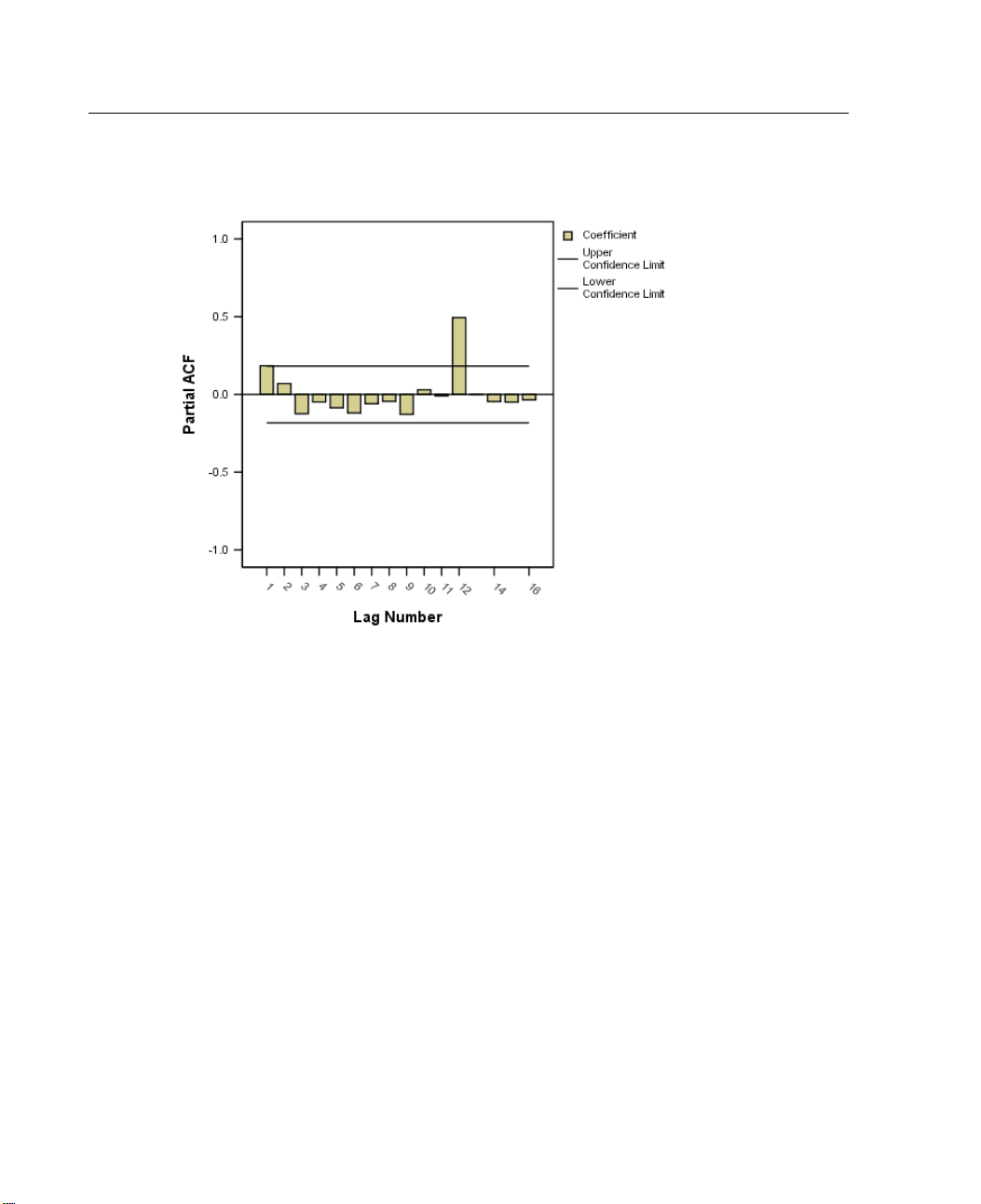
62
Chapter 8
Figure 8-13
Residual partial autocorrelation plot for simple model
The partial autocorrelation function removes the indirect effect of all intervening
lags, providing the best measure of a direct relationship between time series values
separated by a given lag. The partial autocorrelation function for the simple model
shows the same significant peak at a lag of 12 as the autocorrelation function. This
provides definitive proof that the residuals of the simple model contain the structure
of the annual seasonality of the time series.
Summary
Given the poor fit of the simple model to the data and the presence of significant
structure in the model’s residuals, you can conclude that the simple model is not
a good choice for modeling the data.
The initial plot of the time series suggested a model with both trend and
seasonality, neither of which is present in the simple model. Next, we will use the
Holt model to extend the present model with a trend component.
Page 77
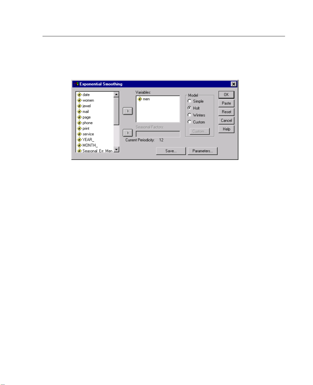
63
Building and Analyzing a Holt Model
Figure 8-14
Exponential
E To build a Holt model, open the Exponential Smoothing dialog box.
E Select Holt in the Model group.
E Click Parameters.
Smoothing dialog box
Exponential Sm
oothing
Page 78
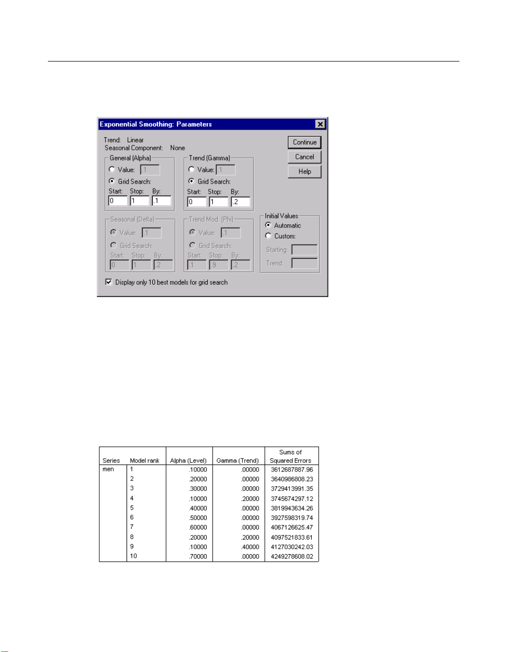
64
Chapter 8
Figure 8-15
Exponential Smoothing Parameters dialog box
E SelectGrid Search in both the General (Alpha) and Trend (Gamma) groups. Leave the
Start, S
top, and By text boxes with their default values.
The current grid search results in evaluating 66 models, one for each of the possible
combinations of alpha and gamma—11 values of alpha and 6 values of gamma.
E Click Continue.
E Click OK in the Exponential Smoothing dialog box.
Figure 8-16
Exponential smoothing, linear trend and no seasonality
Page 79
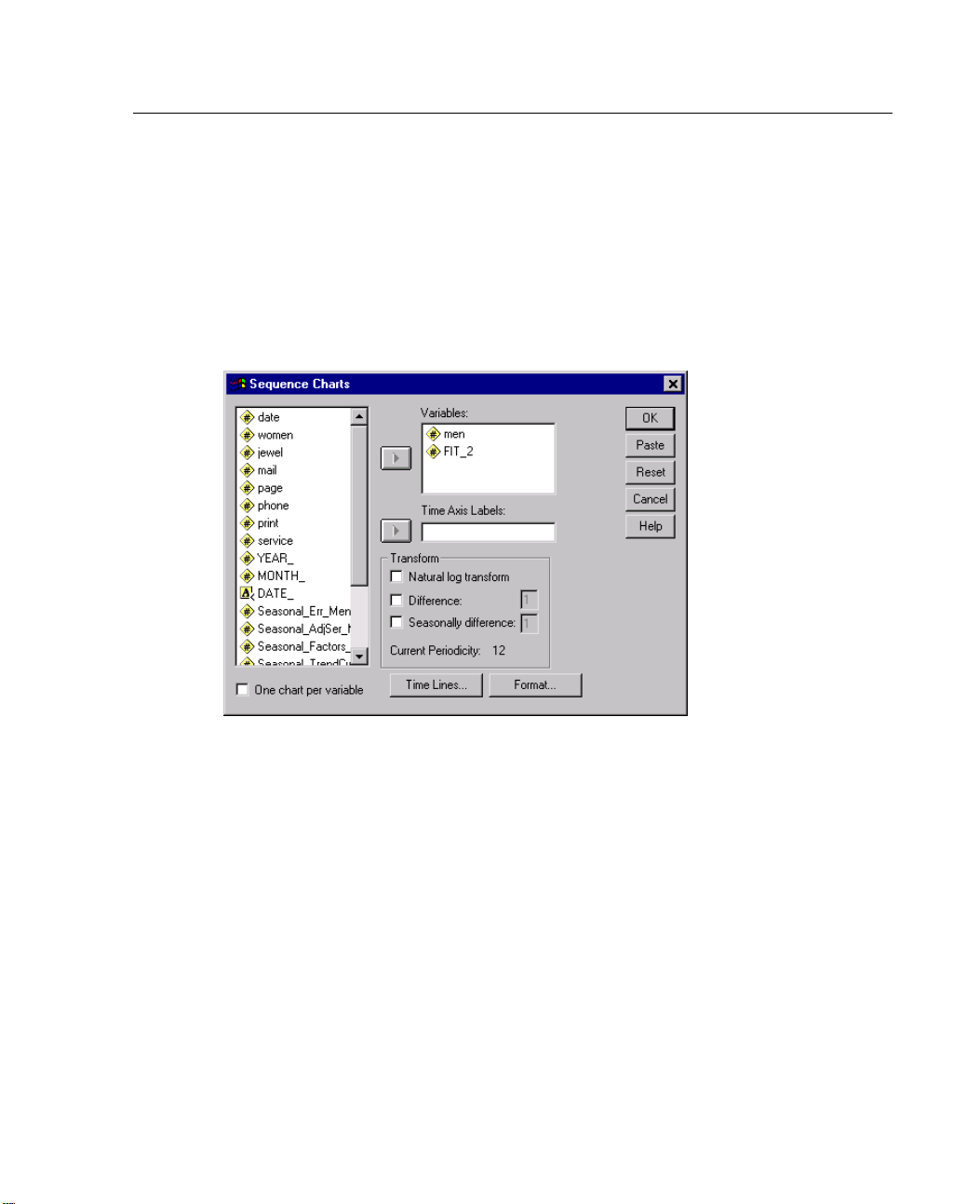
65
Exponential Sm
oothing
The SSE measure of error is lowest when alpha is 0.1 and gamma is 0. The low
values of alpha and gamma mean that all observations have roughly equal weight in
modeling bo
th the overall level of the series and the series trend. The SSE for the
best-fitting Holt model is 3612687888, which is slightly better than the SSE for the
best-fitting simple model of 3716115994. The Holt model then appears to give a
better fit
Figure 8-17
Sequence Charts dialog box
tothedatathanthesimplemodel.
E To see how well the Holt model fits the data, open the Sequence Charts dialog box.
E Deselect the variable associated with the simple model (FIT_1) from the Variables list
and select the variable corresponding to the Holt model (FIT_2).
E Click OK.
Page 80
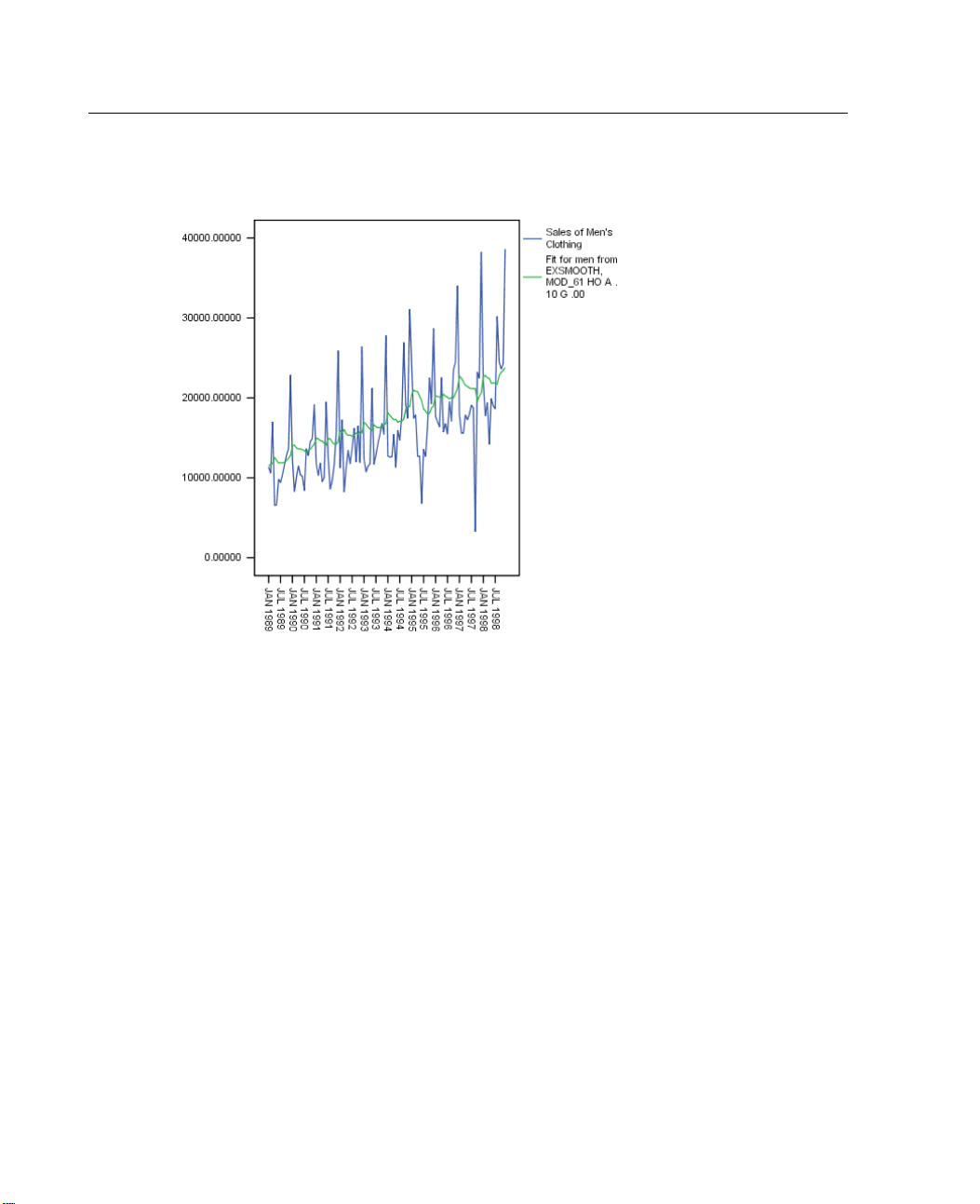
66
Chapter 8
Figure 8-18
Predictions from exponential smoothing, linear trend and no seasonality
Notice that the model does a good job of capturing the trend component of the data.
As expected, though, it does not account for the observed seasonality. As in the case
of the simple model, examination of the autocorrelations and partial autocorrelations
of the residuals provides more quantitative insight.
Page 81
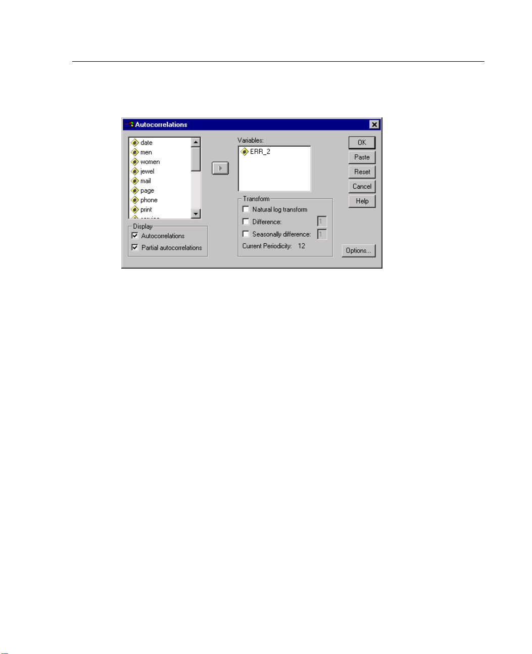
67
Exponential Sm
Figure 8-19
Autocorrelations dialog box
E Examine the autocorrelations of the residuals by opening the Autocorrelations
oothing
dialog box.
E Deselect the variable associated with the simple model (ERR_1) from the Variables
list and
E Click O
select the variable corresponding to the Holt model (ERR_2).
.
K
Page 82
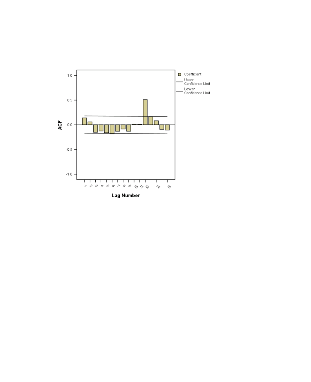
68
Chapter 8
Figure 8-20
Residual autocorrelation plot for Holt model
The autocorrelation function shows a significant peak at a lag of 12, just as in the
case of the simple model. This is no surprise, since the Holt model (like the simple
model) doesn’t account for seasonality.
Page 83
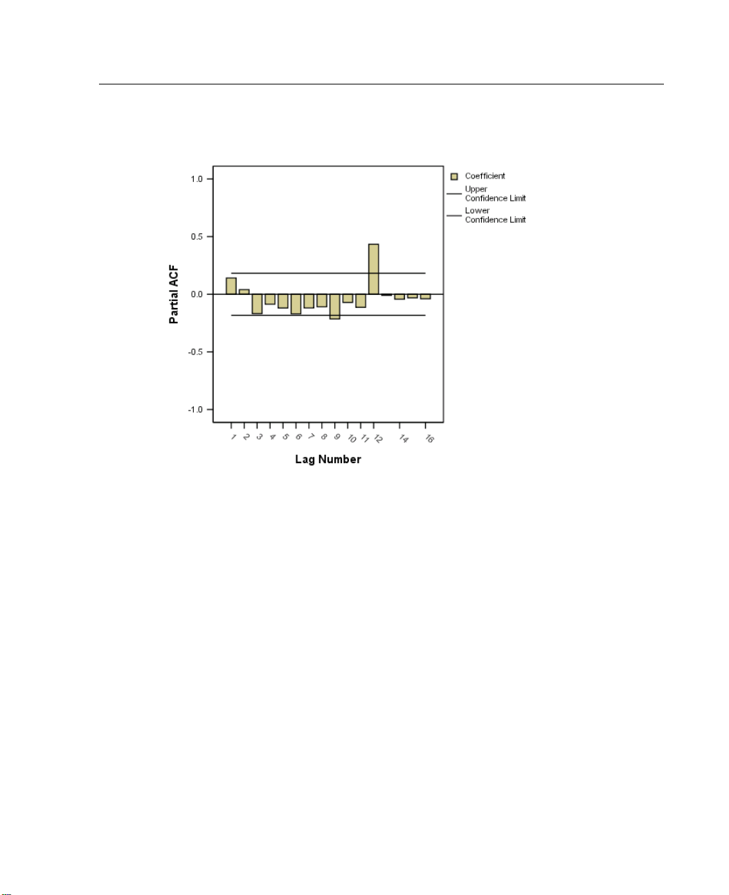
69
Figure 8-21
Residual partial autocorrelation plot for Holt model
Exponential Sm
oothing
The partial autocorrelation function for the Holt model exhibits the same significant
peak at a lag of 12 as the autocorrelation function. This shows that the residuals of
the Holt model, like those of the simple model, contain the structure of the annual
seasonality of the time series.
Summary
Given the presence of significant structure in the residuals of the Holt model
corresponding to the seasonality component, you can conclude that the Holt model,
although better than the simple model, is not a good choice for modeling the data.
Recall that the initial plot of men’s clothing sales over time suggested a model
incorporating a linear trend and multiplicative seasonality—a Winters model.
Page 84
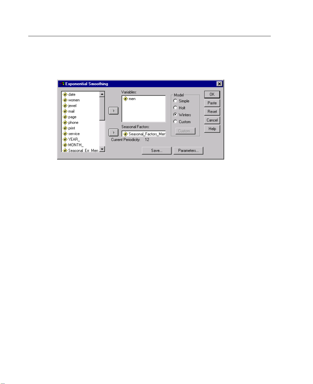
70
Chapter 8
Building and Analyzing a Winters Model
Figure 8-22
Exponential
E To build a Winters model, open the Exponential Smoothing dialog box.
E Select Winters in the Model group.
E Select Seasonal_Factors_Men and move it into the Seasonal Factors list.
E Click Parameters.
Smoothing dialog box
Page 85
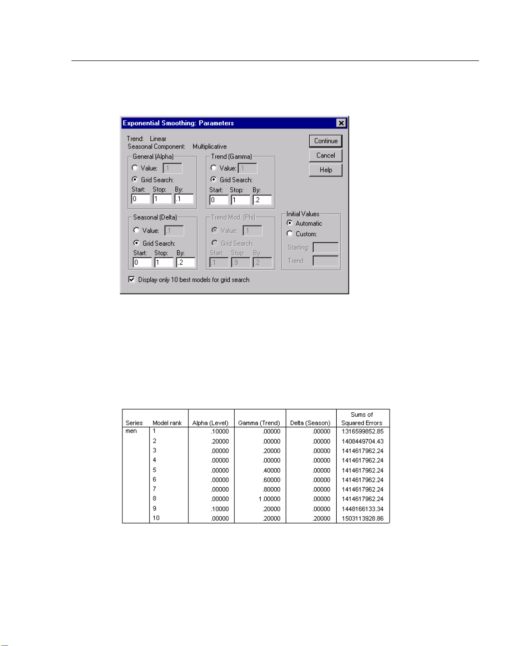
71
Exponential Sm
Figure 8-23
Exponential Smoothing Parameters dialog box
E Select Grid Search in the General (Alpha), Trend (Gamma), and Seasonal (Delta)
groups.
E Click C
Leave the Start, Stop, and By text boxes with their default values.
.
ontinue
oothing
in the Exponential Smoothing dialog box.
E Click O
Figure 8-24
Exponential smoothing, linear trend and multiplicative seasonality
K
Page 86
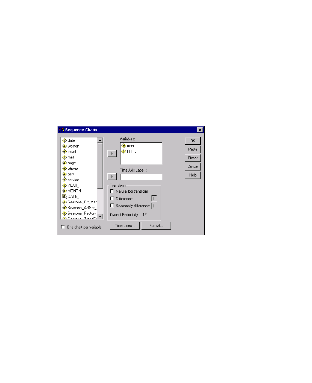
72
Chapter 8
The SSE measure o f error is lowest when alpha is 0.1, gamma is 0, and delta is 0.
The low values of alpha, gamma, and delta mean that all observations have roughly
equal weigh
t in modeling the overall level of the series, the series trend, and the
seasonality. The SSE for the best-fit Winters model is significantly less than the
corresponding values for both the Holt (SSE of 3612687888) and simple (SSE of
371611599
4) models. This is the first indication that the Winters model provides a
substantially better fit to the data.
Figure 8-2
Sequence C
E To see how well the Wintersmodel fits the data, open the Sequence Charts dialog box.
E Deselect the variable associated with the Holt model (FIT_2) from the Variables list
and se
E Clic
5
harts dialog box
lect the variable corresponding to the Winters model (FIT_3).
OK.
k
Page 87
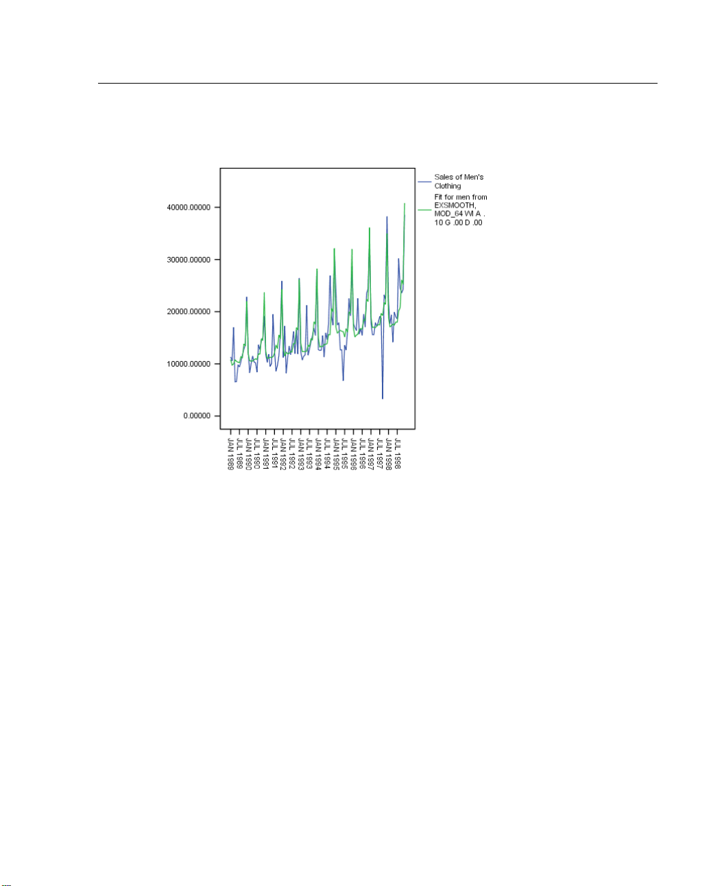
73
Exponential Sm
Figure 8-26
Predictions from exponential smoothing, linear trend and multiplicative seasonality
oothing
Notice that the model does a good job of capturing both the trend and the seasonality
of the data. The data set covers a period of 10 years and includes 10 seasonal peaks
occurring in December of each year. The 10 peaks present in the predicted results
match up well with the 10 annual peaks in the real data.
The results also underscore the limitations of the Exponential Smoothing procedure,
since there is significant structure that is not accounted for. If you are primarily
interested in modeling a long-term trend with seasonal variation, then exponential
smoothing may be a good choice. To model a more complex structure, consider
using the ARIMA procedure. An examination of the autocorrelations and partial
autocorrelations of the residuals will provide stronger evidence for or against the
Winters model.
Page 88
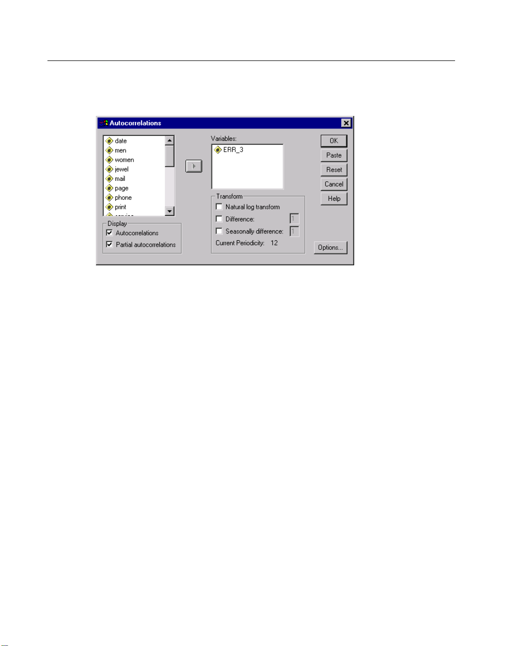
74
Chapter 8
Figure 8-27
Autocorrelations dialog box
E Examine the autocorrelations of the residuals by opening the Autocorrelations
dialog box.
E Deselect the variable associated with the Holt model (ERR_2) from the Variables list
and sele
ct the variable corresponding to the Winters model (ERR_3).
E Click O
.
K
Page 89
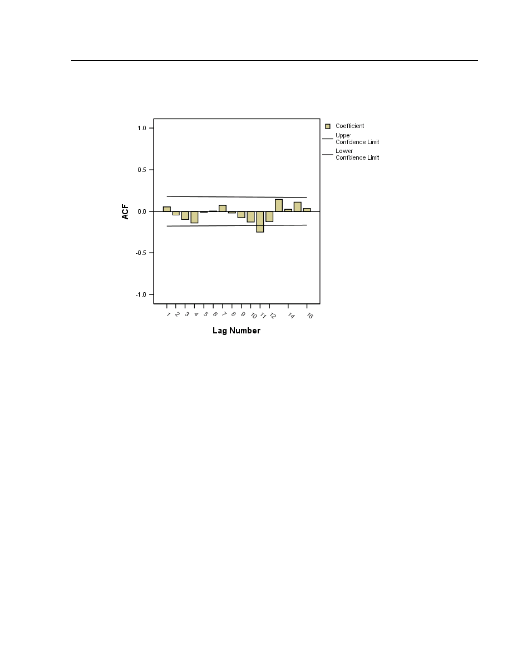
75
Figure 8-28
Residual autocorrelation plot for Winte r s model
Exponential Sm
oothing
The Winters model has adequately described the annual seasonal component, so there
is no longer a significant peak at a lag of 12 in the autocorrelation function; the
peak is within the confidence bounds.
Page 90
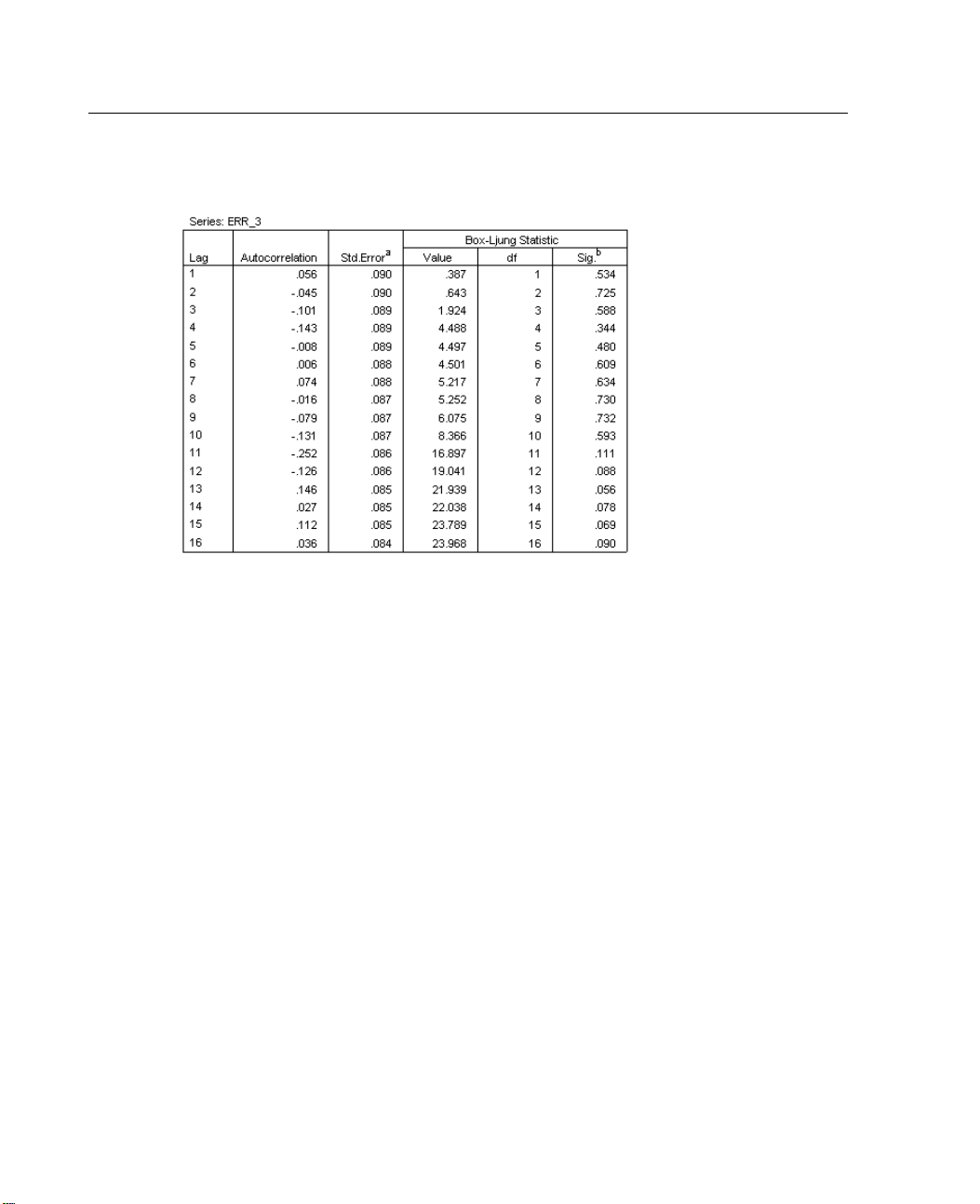
76
Chapter 8
Figure 8-29
Residual autocorrelation statistics for Winters model
Notice also that the Box-Ljung statistic a t a lag of 12 is no longer statistically
significant.
Page 91
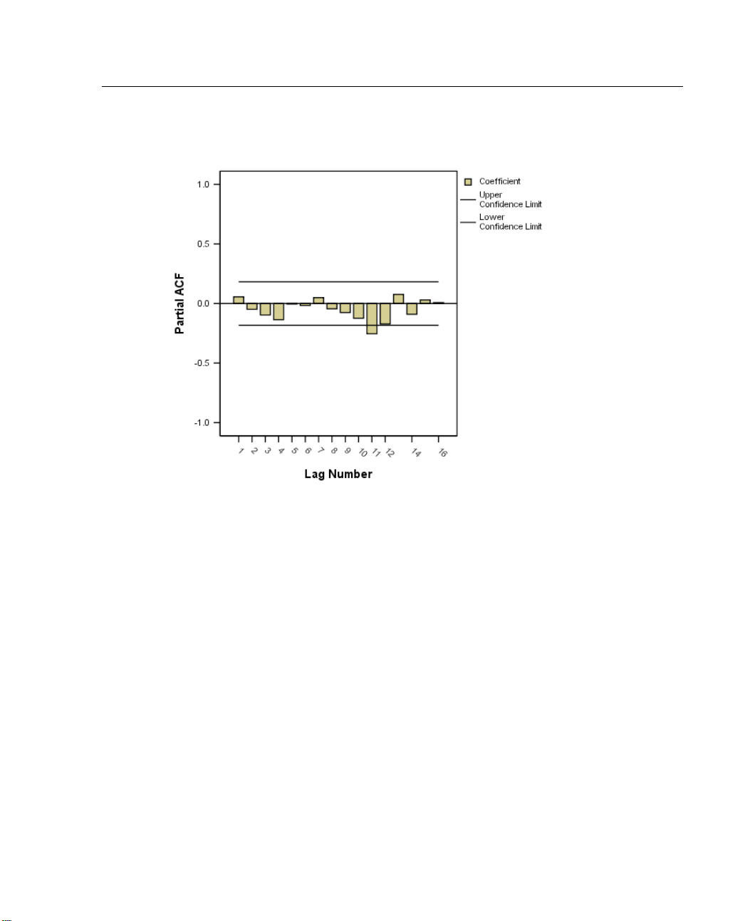
77
Figure 8-30
Residual partial autocorrelation plot for Winters model
Exponential Sm
oothing
The partial autocorrelation function no longer has a significant peak at a lag of 12.
The pea
k at a lag of 11, however, is outside the confidence limits and appears
significant. This would suggest periodic behavior with an 11-month cycle.
The Box-Ljung statistic at a lag of 11, however, isn’t statistically significant. In
on, analysis of the catalog company’s records shows no good business reason to
additi
expect an 11-month cycle. With reasonable confidence, you can then reject the lag
11 peak as irrelevant.
Summa
ry of Model Building
models incorporating different assumptions about trend and seasonality have
Three
been considered, and the results clearly indicate a Winters model over a Holt or
simple model. Not only does the best-fit Winters model give a good visual fit to
ata, but the residuals, as analyzed through their autocorrelations and partial
the d
autocorrelations, show no significant structure.
Page 92

78
Chapter 8
Although the initial plot of the time series suggested linear trend and multiplicative
seasonality, a more thorough analysis would also consider a custom model with linear
trend and ad
ditive seasonality. The results of that analysis show, however, that the
SSE for the best-fit Winters model is lower, giving us confidence that the Winters
model is truly the best exponential smoothing model for our data.
Testing the Predictive Ability of the Model
You can judge the forecasting performance of your model by using holdouts. A
holdout is a historical series point that is not used in the computation of the model
parameter
model to predict values that you actually know, you get an idea of how well the model
forecasts. This method can be illustrated by holding out the data from January, 1998,
through D
model, and the model i s then used to forecast sales in 1998.
To perform a holdout analysis, first select the modeling period:
s, thus removing its effect on the computation of forecasts. By forcing the
ecember, 1998. The data prior to January, 1998, are used to build the
E From the menus choose:
Data
Select Cases...
Page 93
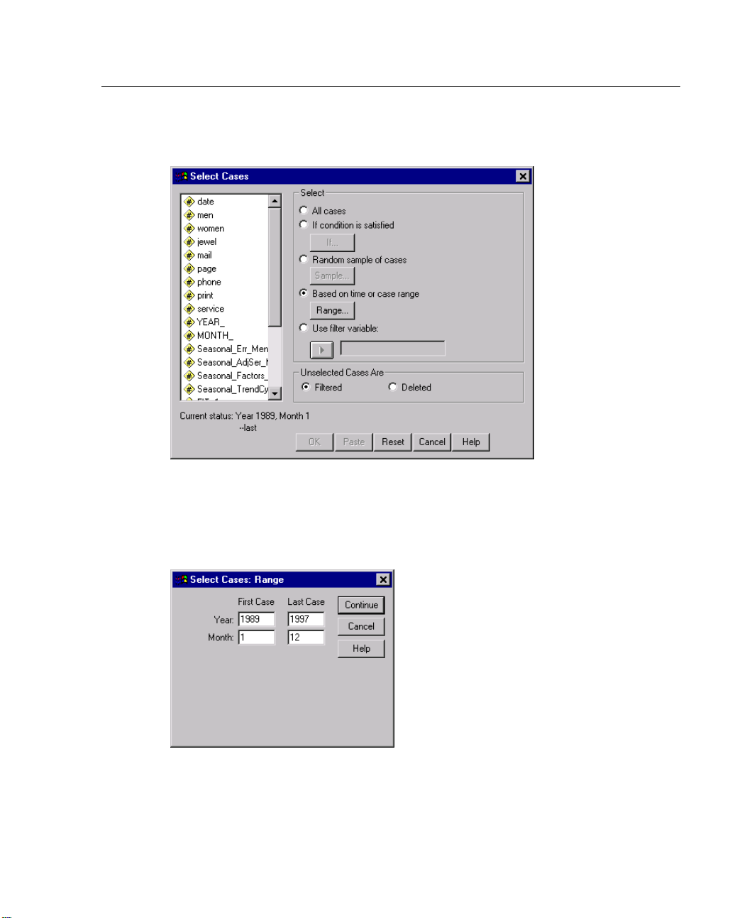
79
Figure 8-31
Select Cases dialog box
Basedontimeorcaserangein the Select group.
E Selec
t
Exponential Sm
oothing
.
E Click R
Figure 8-32
Select Cases Range dialog box
E Enter 1989 for the year associated with the first case and 1 for the month associated
ange
with the first case.
Page 94
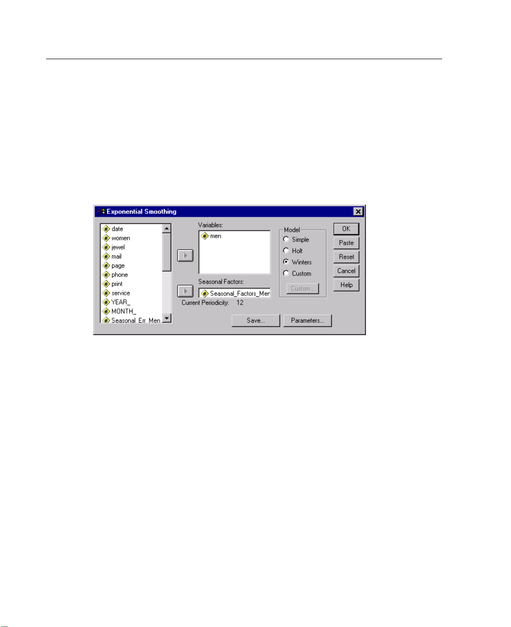
80
Chapter 8
E
Enter 1997 for the year associated with the last case and 12 for the month associated
with the last case.
These choice
E Click Conti
E Click OK in t
Figure 8-33
Exponential Smoothing dialog box
E Open the Exponential Smoothing dialog box.
E Click OK.
s will result in a model based on the period 01/1989 through 12/1997.
.
nue
he Select Cases dialog box.
This results in rerunning the Winters model using the data from 01/1989 to 12/1997
to determi
ne the best-fit parameters. The analysis also includes predictions of sales of
men’s clothing during the holdout period (01/1998 to 12/1998) using the parameters
from the best-fit model.
Page 95
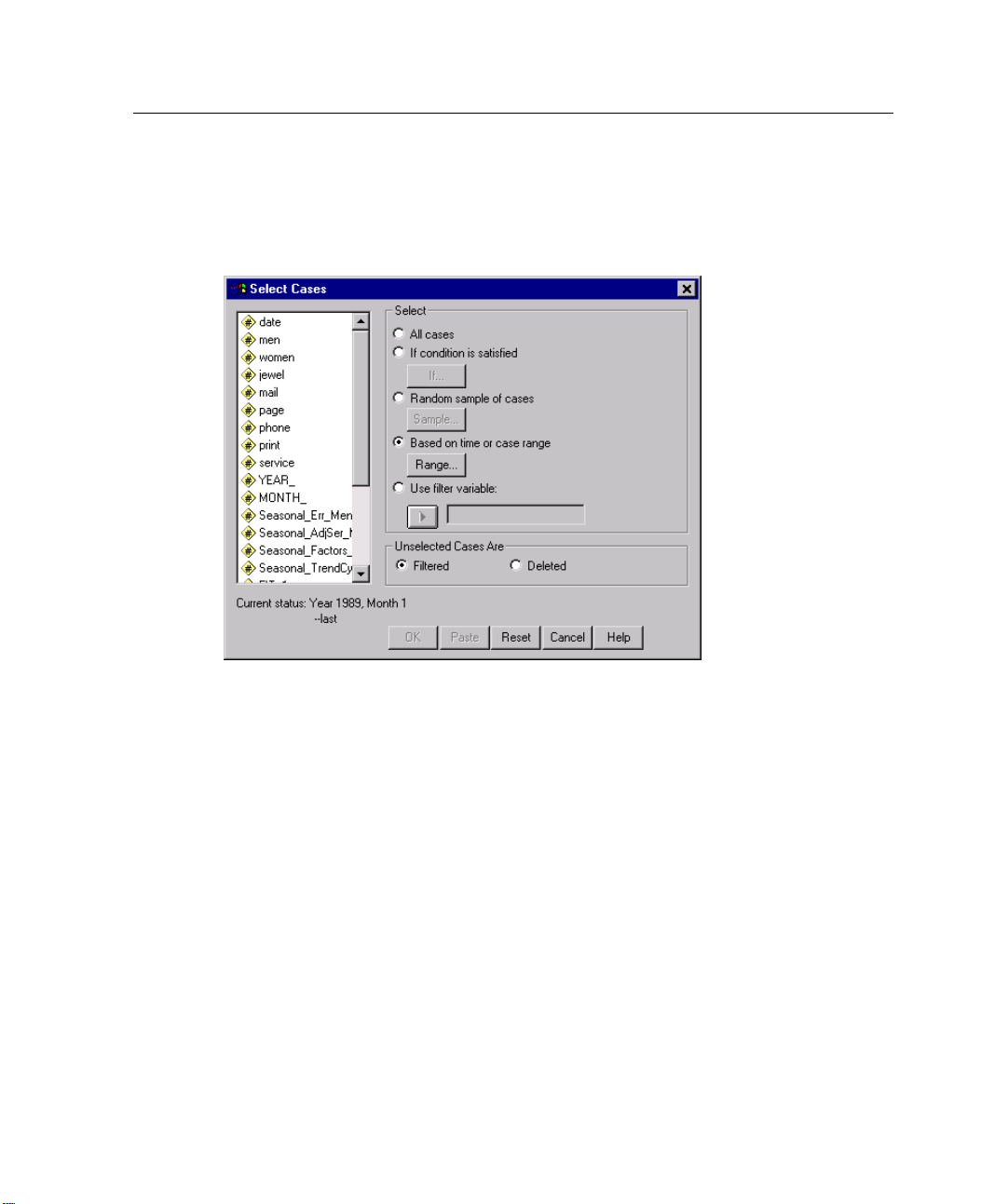
81
Exponential Sm
oothing
Comparison of the model predictions for the holdout period with the actual data is
best done by limiting the cases to the holdout period itself.
Figure 8-34
Select Cases dialog box
E Open t
E Click
he Select Cases dialog box.
Range.
Page 96
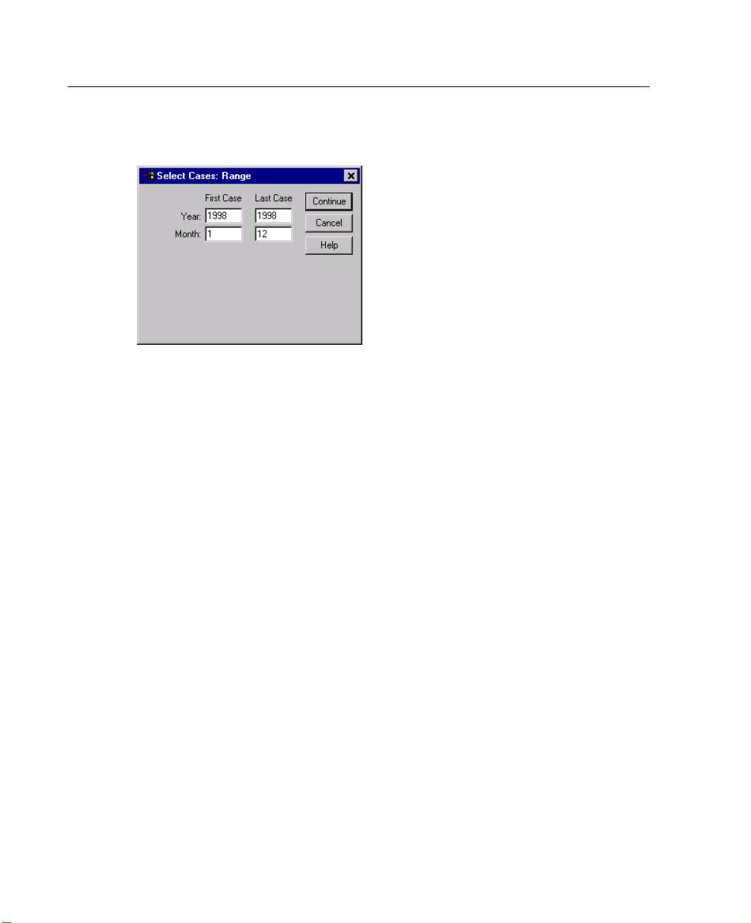
82
Chapter 8
Figure 8-35
Select Cases Range dialog box
E Enter 1998 for the year associated with the first case and 1 for the month associated
with the first case.
E Enter 1998 for the year associated with the last case and 12 for the month associated
with the last case.
E Click Continue.
E Click OK in the Select Cases dialog box.
Page 97
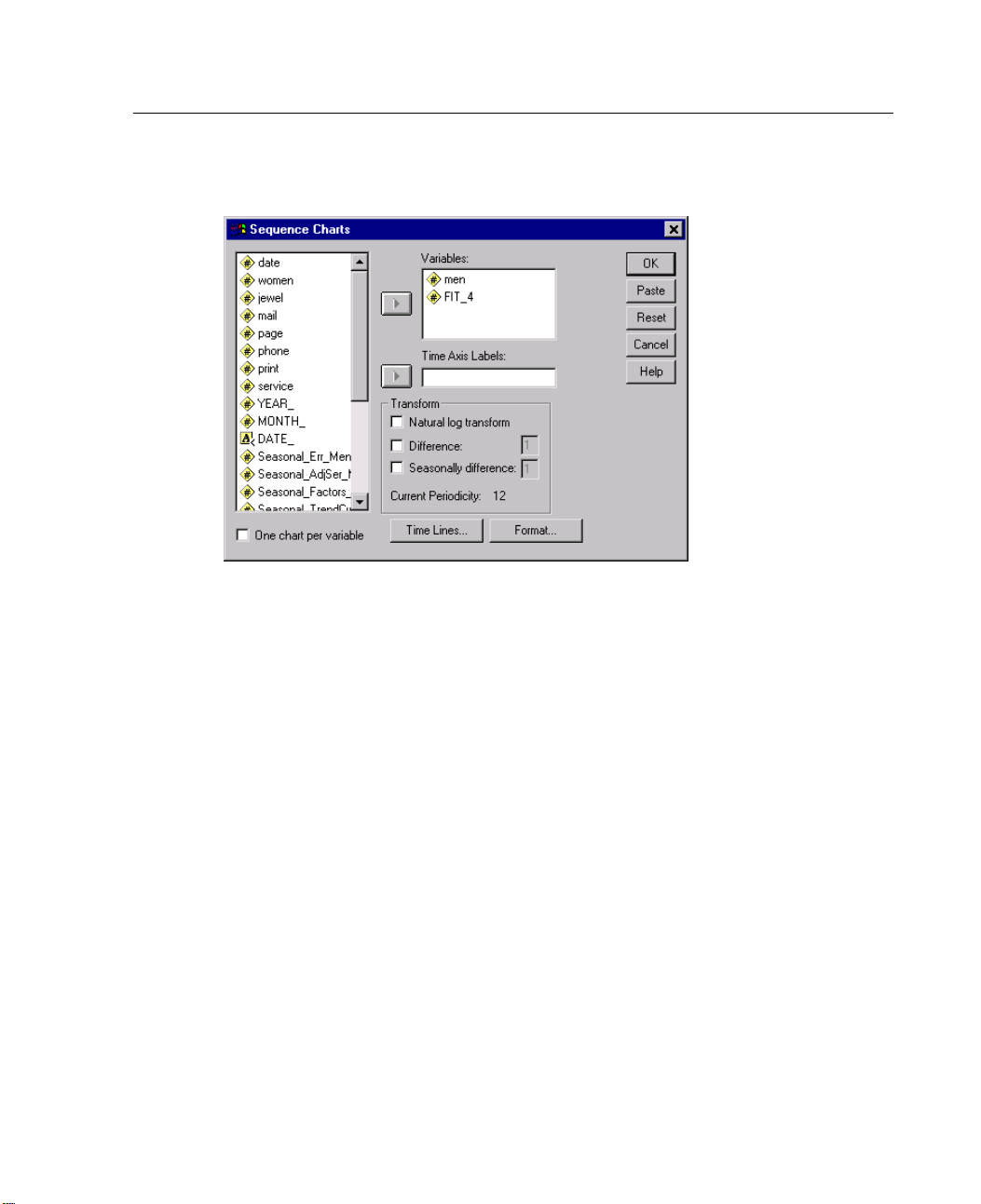
83
Exponential Sm
Figure 8-36
Sequence Charts dialog box
E Open th
E Desele
e Sequence Charts dialog box.
ct the variable associated with the original Winters model (FIT_3) from
the Variables list and select the variable corresponding to the Winters model with
holdouts (FIT_4).
oothing
E Click OK.
Page 98
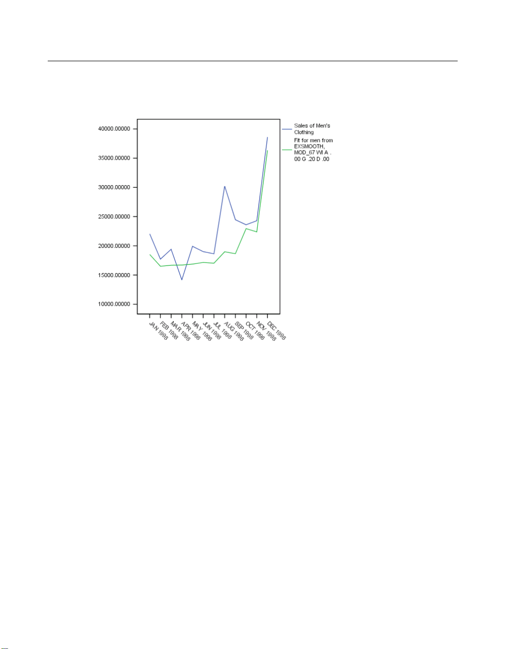
84
Chapter 8
Figure 8-37
Forecast from Winters model w ith holdouts
han the value for August, 1998, the forecast values show good agreement
Other t
with the known values, indicating that the model has satisfactory predictive ability.
A review of the company records shows that a 20%-off promotion was in effect for
the mai
ling of August, 1998, which may explain why sales were unusually high for
that month. You expect that the model will behave well in the absence of special
events such as occasional promotions but may need to be modified if accounting
ecialeventsisimportant.
for sp
Using the Model to P redict Future Sales
You’ve determined that a Winters model is the best exponential smoothing model for
data and obtained satisfactory results regarding its predictive ability. Now it’s
your
time to use the model to predict future sales.
Page 99
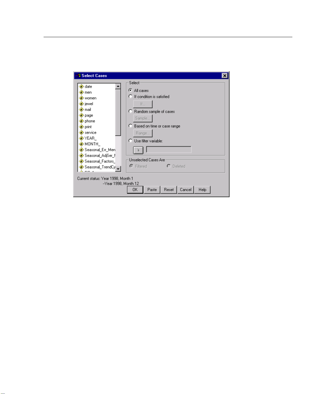
85
Figure 8-38
Select Cases dialog box
To pred
ict future values of sales of men’s clothing, first include all cases by
performing the following steps:
Exponential Sm
oothing
E Open the Select Cases dialog box.
E Select All Cases in the Select group.
E Click OK.
Page 100
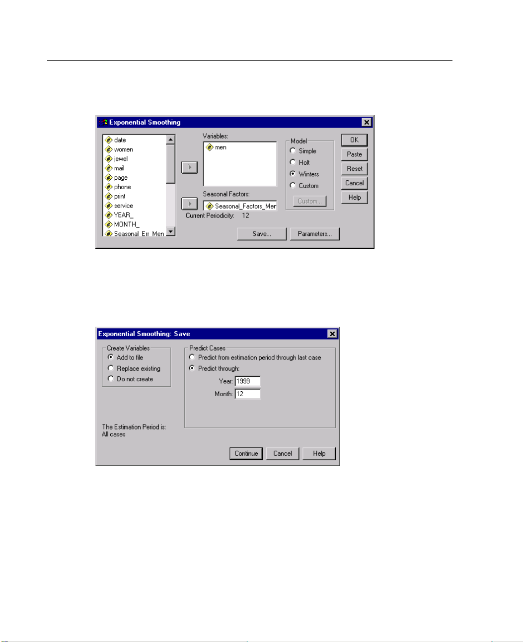
86
Chapter 8
Figure 8-39
Exponential Smoothing dialog box
E Open the
E Click Sa
Figure 8-40
Exponential Smoothing Save dialog box
E Select Addtofilein the Create Variables group.
Exponential Smoothing dialog box.
.
ve
This causes the forecast values to be saved as regular variables in your working
data file.
E Select Predict through in the Predict Cases group.
E Enter 1999 for the year and 12 for the month.
 Loading...