Spss REGRESSION MODELS 12.0 User Manual

™

SPSS Regre

ssion Models

12.0

For more information about SPSS®software products, please visit our Web site at

http://www.

SPSS Inc.
233 South Wacker Drive, 11th Floor
Chicago, IL 60
Tel: [phone]
Fax: [phone]

SPSS is a regis
of SPSS Inc. for its proprietary computer software. No material describing such
software may be produced or distributed without the written permission of the
owners of the
the published materials.

The SOFTWARE and documentation are provided with RESTRICTED RIGHTS.
Use, duplica
in subdivision (c) (1) (ii) of The Rights in Technical Data and Computer Software
clause at 52.227-7013. Contractor/manufacturer is SPSS Inc., 233 South Wacker
Drive, 11th

General notice: Other product names mentioned herein are used for identification
purposes only and may be trademarks of their respective companies.

TableLook i
Windows is a registered trademark of Microsoft Corporation.
DataDirect, DataDirect Connect, INTERSOLV, and SequeLink are registered
trademarks
Portions of this product were created using LEADTOOLS © 1991-2000, LEAD
Technologies, Inc. ALL RIGHTS RESERVED.
LEAD, LEADTO
Technologies, Inc.
Portions of this product were based on the work of the FreeType Team
(http://ww

SPSS Regression Models™ 12.0
Copyright © 2003 by SPSS Inc.
All rights re
Printed in the United States of America.

No part of this publication may be reproduced, stored in a retrieval system, or
transmitted
recording, or otherwise, without the prior written permission of the publisher.

spss.com or contact

606-6412

tered trademark and the other product names are the trademarks

trademark and license rights in the software and the copyrights in

tion, or disclosure by the Government is subject to restrictions as set forth

Floor, Chicago, IL 60606-6412.

s a trademark of SPSS Inc.

of DataDirect Technologies.

OLS, and LEADVIEW are registered trademarks of LEAD

w.freetype.org).

served.

, in any form or by any means, electronic, mechanical, photocopying,

Preface

SPSS 12.0 is a powerful software package for microcomputer data management and
analysis. The Regression Models option is an add-on enhancement that provides

nal statistical analysis techniques. The procedures in Regression Models must

additio
be used with the SPSS 12.0 Base and are completely integrated into that system.

The Regression Models option includes procedures for:

 Logistic regression
 Multinomial logistic regression
 Nonlinear regression
 Weighted least-squares regression
 Two-stage least-squares regression

ation

Install

To insta
features in the installation instructions supplied with the SPSS Base. (To start,
double-click on the SPSS Setup icon.)

Compatibility

SPSS is designed to run on many computer systems. See the materials that came with
your system for specific information on minimum and recommended requirements.

ll Regression Models, follow the instructions for adding and removing

iii

Serial Numbers

Your serial number is your identification number with SPSS Inc. You will need
this serial number when you contact SPSS Inc. for information regarding support,
payment, or a

n upgraded system. The serial number was provided with your Base

system.

Customer Se

If you have a

rvice

ny questions concerning your shipment or account, contact your local
office, listed on the SPSS Web site at http://www.spss.com/worldwide. Please have
your serial number ready for identification.

Training Seminars

SPSS Inc. provides both public and onsite training seminars. All seminars feature
hands-on workshops. Seminars will be offered in major cities on a regular basis. For
more infor

mation on these seminars, contact your local office, listed on the SPSS

Web site at http://www.spss.com/worldwide.

Technica

The servi

l Support

ces of SPSS Technical Support are available to registered customers.
Customers may contact Technical Support for assistance in using SPSS products
or for installation help for one of the supported hardware environments. To reach
Technic

al Support, see the SPSS Web site at http://www.spss.com, or contact your
local office, listed on the SPSS Web site at http://www.spss.com/worldwide.Be
prepared to identify yourself, your organization, and the serial number of your system.

Additional Publications

Additional copies of SPSS product manuals may be purchased directly from SPSS
Inc. Visit our Web site at http://www.spss.com/estore, or contact your local SPSS

, listed on t he SPSS Web site at http://www.spss.com/worldwide. For telephone

office
orders in the United States and Canada, call SPSS Inc. at 800-543-2185. For
telephone orders outside of North America, contact your local office, listed on the
SPSS We

bsite.

iv

The SPSS Statistical Procedures Companion, by Marija Norušis, is being prepared
for publication by Prentice Hall. It contains overviews of the procedures in the SPSS
Base, plus Lo

gistic Regression, General Linear Models, and Linear Mixed Models.

Further information will be available on the SPSS Web site at http://www.spss.com

Store, select your country, and click Books).

(click

Tell Us Your Thou ghts

Your comments are important. Please send us a letter and let us know about your
experiences with SPSS p roducts. We especially like to hear about new and interesting
applicati

ons using the SPSS system. Please send e-mail to [email protected] or
write to SPSS Inc., Attn.: Director of Product Planning, 233 South Wacker Drive,
11th Floor, Chicago, IL 60606-6412.

About This Manual

This manual documents the graphical user interface for the procedures included in
the Regression Models module. Illustrations of dialog boxes are taken from SPSS
for Windo

ws. Dialog boxes in other operating systems are similar. The Regression
Models command syntax is included in the SPSS 12.0 Command Syntax Reference,
available on the product CD-ROM.

Contacting SPSS

If you would like t o be on our mailing list, contact one of our offices, listed on
our Web site at http://www.spss.com/worldwide. We will send you a copy of our
newslet

ter and let you know about SPSS Inc. activities in your area.

v

Contents

1 Choosing a Pr

ocedure for Binary Logistic

Regression Models 1

2 Logistic Regression 3

LogisticRegressionDataConsiderations ......................... . 4

ObtainingaLogisticRegressionAnalysis ......................... . 4

LogisticRegressionVariableSelectionMethods.................... . 6

LogisticRegressionDefineCategoricalVariables................... . 7

LogisticRegressionSaveNewVariables ......................... . 9

LogisticRegressionOptions................................... .10

LOGISTICREGRESSIONCommandAdditionalFeatures............... .11

3 Multinomial Logistic Regression 13

MultinomialLogisticRegressionDataConsiderations................ .13

ObtainingaMultinomialLogisticRegression....................... .14

MultinomialLogisticRegressionModels.......................... .15

MultinomialLogisticRegressionReferenceCategory................ .17

MultinomialLogisticRegressionStatistics........................ .18

MultinomialLogisticRegressionCriteria.......................... .19

MultinomialLogisticRegressionOptions.......................... .21

MultinomialLogisticRegressionSave............................ .22

NOMREGCommandAdditionalFeatures.......................... .23

vii

4 Probit Analysis 25

robitAnalysisDataConsiderations............................. .25

P

btainingaProbitAnalysis.................................... .26

O

robitAnalysisDefineRange.................................. .28

P

robitAnalysisOptions....................................... .28

P

ROBITCommandAdditionalFeatures........................... .29

P

5N

onlinear Regression 31

NonlinearRegressionDataConsiderations........................ .32

ObtainingaNonlinearRegressionAnalysis........................ .32

NonlinearRegressionParameters .............................. .34

NonlinearRegressionCommonModels .......................... .35

NonlinearRegressionLossFunction............................. .36

NonlinearRegressionParameterConstraints...................... .37

NonlinearRegressionSaveNewVariables........................ .38

NonlinearRegressionOptions ................................. .39

InterpretingNonlinearRegressionResults........................ .40

NLRCommandAdditionalFeatures.............................. .40

6 Weight Estimation 43

WeightEstimationDataConsiderations .......................... .43

ObtainingaWeightEstimationAnalysis .......................... .44

WeightEstimationOptions.................................... .46

WLSCommandAdditionalFeatures ............................. .46

viii

7 Two-Stage Least-Squares Regression 47

wo-Stage Least-Squares Regression Data Considerations . . . . . . . . . . . . 48

T

btaining a Two-Stage Least-Squares Regression Analysis . . . . . . . . . . . . 48

O

wo-StageLeast-SquaresRegressionOptions..................... .50

T

SLSCommandAdditionalFeatures............................. .50

2

Appendix

A Categorical Variable Coding Schemes 51

Deviation................................................. .51

Simple ................................................... .52

Helmert .................................................. .53

Difference ................................................ .54

Polynomial................................................ .54

Repeated................................................. .55

Special .................................................. .56

Indicator ................................................. .57

Index 59

ix

Chapter

1

ChoosingaPr

ocedure for Binary

Logistic Regression Models

Binary log
procedure or the Multinomial Logistic Regression procedure. Each procedure has
options not available in the other. An important theoretical distinction is that the
Logistic R
and goodness-of-fit tests using data at the individual case level, regardless of how the
data are entered and whether or not the number of covariate patterns is smaller than the
total num
aggregates cases to form subpopulations with identical covariate patterns for the
predictors, producing predictions, residuals, and goodness-of-fit tests based on these
subpopu
on only a limited number of values—so that there are several cases at each distinct
covariate pattern—the subpopulation approach can produce valid goodness-of-fit tests
and inf

istic regression models can be fitted using either the Logistic Regression

egression procedure produces all predictions, residuals, influence statistics,

ber of cases, while the Multinomial Logistic Regression procedure internally

lations. If all p redictors are categorical or any continuous predictors take

ormative residuals, while the individual case level approach cannot.

ic Regression

Logist

 Hosme
 Stepw
 Contra
 Altern
 Classi
 Model f
 Saves p

provides the following unique features:

r-Lemeshow test of goodness of fit for the model

ise analyses

sts to define model parameterization
ative cut points for classification
fication plots

itted on one set of cases to a held-out set of cases

redictions, residuals, and influence statistics

1

2

Chapter 1

Multinomial Log istic Regression provides the following unique features:

 Pearson and deviance chi-square tests for goodness of fit of the model
 Specification of subpopulations for grouping of data for goodness-of-fit tests
 Listing of counts, predicted counts, and residuals by subpopulations
 Correction of variance estimates for over-dispersion
 Covariance matrix of the parameter estimates
 Tests of linear combinations of parameters
 Explicit specification of nested models
 Fit 1-1 matched conditional logistic regression models using differenced variables

Chapter

2

Logistic Reg

Logistic regression is useful for situations in which you want to be able to predict
the presenc
predictor variables. It is similar to a linear regression model but is suited to models
where the dependent variable is dichotomous. Logistic regression coefficients can
be used to e
Logistic regression is applicable to a broader range of research situations than
discriminant analysis.

Example.

(CHD)? Given a sample of patients measured on smoking status, diet, exercise,
alcohol use, and CHD status, you could build a model using the four lifestyle variables
to predic
then be used to derive estimates of the odds ratios for each factor to tell you, for
example, how much more likely smokers are to develop CHD than nonsmokers.

Statist

categorical variable: parameter coding. For each step: variable(s) entered or
removed, iteration history, –2 log-likelihood, goodness of fit, Hosmer-Lemeshow
goodne
table, correlations between variables, observed groups and predicted probabilities
chart, residual chi-square. For each variable in the equation: coefficient (B), standard
error o
exp(B), log-likelihood if term removed from model. For each variable not in the
equation: score statistic. For each case: observed group, predicted probability,
predi

e or absence of a characteristic or outcome based on values of a set of

stimate odds ratios for each of the independent variables in the model.

What lifestyle characteristics are risk factors for coronary heart disease

t the presence or absence of CHD in a sample of patients. The model can

ics.

For each analysis: total cases, selected cases, valid cases. For each

ss-of-fit statistic, model chi-square, improvement chi-square, classification

f B, Wald statistic, estimated odds ratio (exp(B)), confidence interval for

cted group, residual, standardized residual.

ression

Methods. You can estimate models using block entry of variables or any of the

following stepwise methods: forward conditional, forward LR, forward Wald,

ard conditional, backward LR, or backward Wald.

backw

3

4

Chapter 2

Logistic Reg

Data. The de

interval level or categorical; if categorical, they should be dummy or indicator coded
(there is an option in the procedure to recode categorical variables automatically).

Assumption

same sense that discriminant analysis does. However, your solution may be more
stable if your predictors have a multivariate normal distribution. Additionally, as
with other
biased estimates and inflated standard errors. The procedure is most effective when
group membership is a truly categorical variable; if group membership is based
on values
should consider using linear regression to take advantage of the richer information
offered by the continuous variable itself.

Related p

for multicollinearity. If assumptions of multivariate normality and equal
variance-covariance matrices are met, you may be able to get a quicker solution using
the Disc
you can also use the Loglinear p rocedure. If your dependent variable is continuous,
use the Linear Regression procedure. You can use the ROC Curve procedure to plot
probab

ression Data Considerations

pendent variable should be dichotomous. Independent variables can be

s.

Logistic regression does not rely on distributional assumptions in the

forms of regression, multicollinearity among the predictors can lead to

of a continuous variable (for example, “high IQ” versus “low IQ”), you

rocedures.

riminant Analysis procedure. If all of your predictor variables are categorical,

ilities saved with the Logistic Regression procedure.

Use the Scatterplot procedure to screen your data

Obtaining a Logistic Regression Analysis

E From the menus choose:

e

Analyz

Regres

Binary

sion

Logistic...

5

Logistic Regre

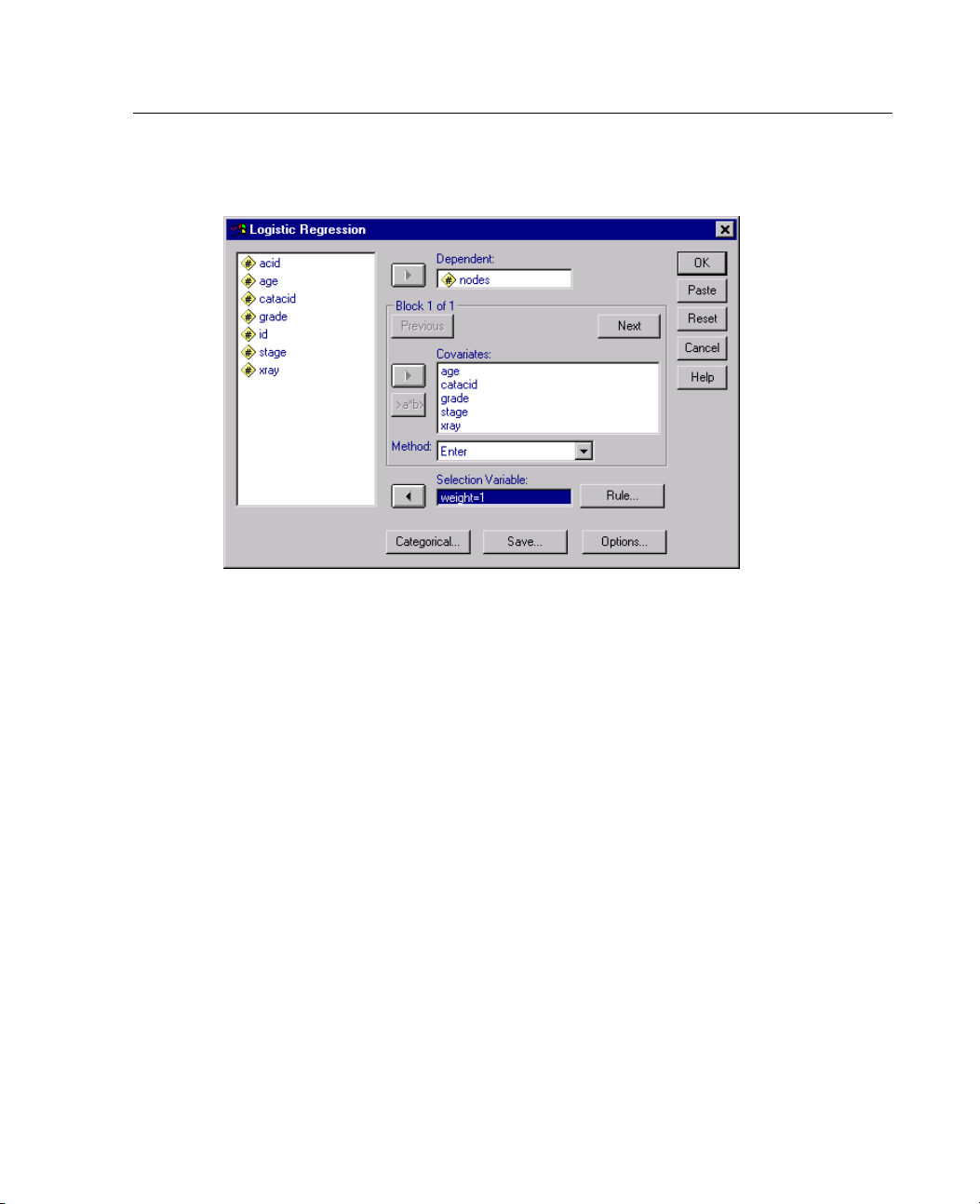
Figure 2-1

Logistic Regression dialog box

E Select one dichotomous dependent variable. This variable may be numeric or short

.

string

ssion

E Select

one or more covariates. To include interaction terms, select all of the variables

involved in the interaction and then select

>a*b>.

To enter variables in groups (blocks), select the covariates for a block, and click

ify a new block. Repeat until all blocks have been specified.

to spec
Optionally, you can select cases for a nalysis. Choose a selection variable, and click

Rule.

Next

6

Chapter 2

Logistic Regression Set Rule

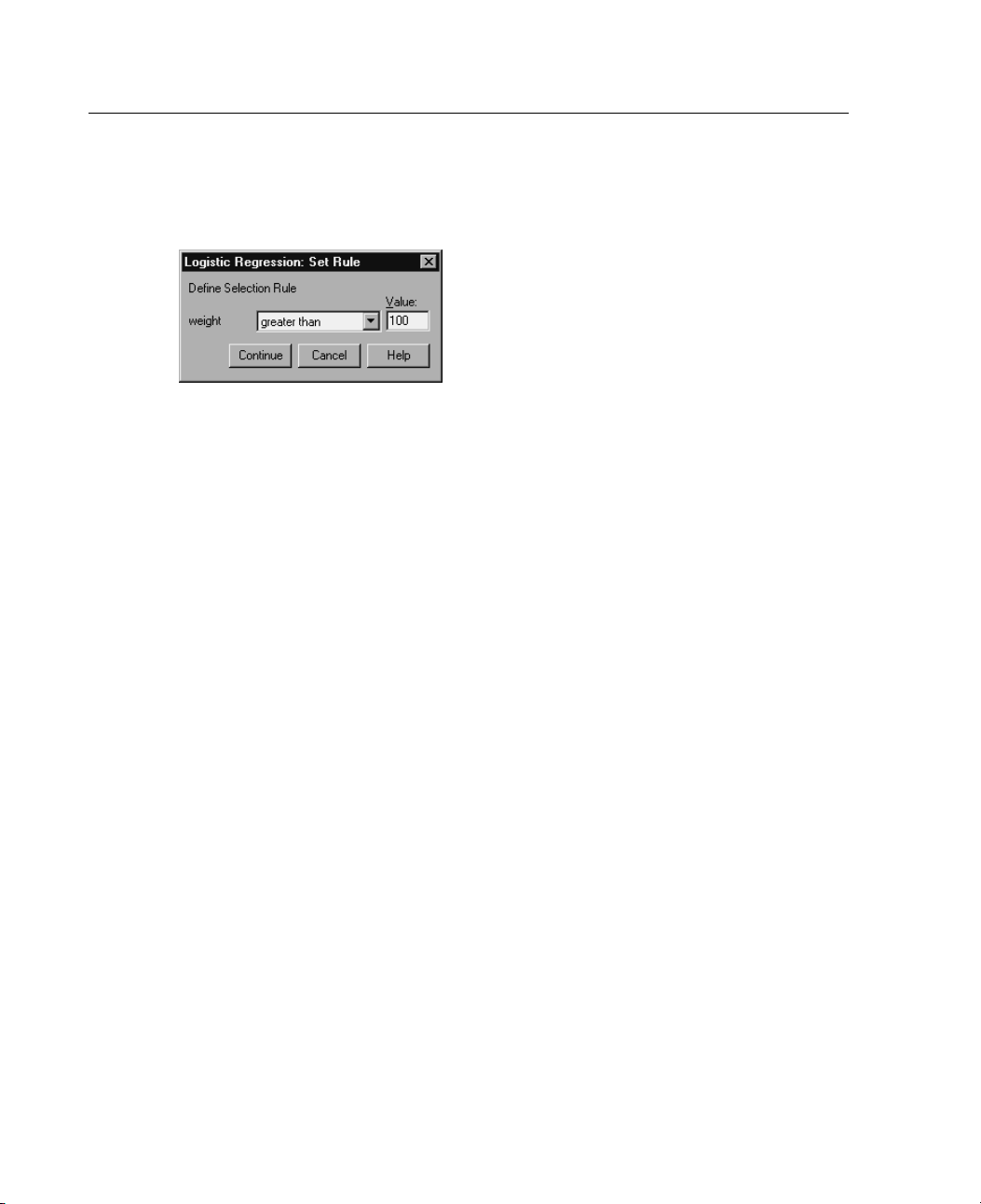
Figure 2-2

Logistic Reg

ression Set Rule dialog box

Cases defined by the selection rule are included in model estimation. For example, if
you select

ed a variable and

equals and specified a value of 5, then only the cases for

which the selected variable has a value equal to 5 are included in estimating the model.

Statistics and classification results are generated for both selected and unselected

cases. Th

is provides a mechanism for classifying new cases based on previously
existing data, or for partitioning your data into training and testing subsets, to perform
validation on the model generated.

Logistic Regression Variable Selection Methods

Method selection allows you to specify how independent variables are entered into
the analysis. Using different methods, you can construct a variety of regression
models f

 Enter.

 Forward Selection (Condit ional). Stepwise selection method with entry testing

 Forwar

 Forwa

rom the same set of variables.

A procedure for variable selection in which all variables in a block are

enteredinasinglestep.

based on the significance of the score statistic, and removal testing based on the
probabi

lity of a likelihood-ratio statistic based on conditional parameter estimates.

d Selection (Likelihoo d Ratio).

Stepwise selection method with entry
testing based on the significance of the score statistic, and removal testing based
on the probability of a likelihood-ratio statistic based on the maximum partial

hood estimates.

likeli

rd Selection (Wald).

Stepwise selection method with entry testing based
on the significance of the score statistic, and removal testing based on the
probability of the Wald statistic.

7



Backward Elimination (Conditional). Backward stepwise selection. Removal

testing is b

ased on the probability of the likelihood-ratio statistic based on

conditional parameter estimates.

 Backward Elimination (Likelih ood Ratio). Backward stepwise selection. Removal

testing is based on the probability of the likelihood-ratio statistic based on the
maximum par

 Backward E

tial likelihood estimates.

limination (Wald).

Backward stepwise selection. Removal testing is

based on the probability of the Wald statistic.

The significance values in your output are based on fitting a single model. Therefore,
the signif

icance values are generally invalid when a stepwise method is used.

All independent variables selected are added to a single regression model.
However, you can specify different entry methods for different subsets of variables.
For exampl

e, you can enter one block of variables into the regression model using
stepwise selection and a second block using forward selection. To add a second block
of variables to the regression model, click

Next.

Logistic Regression Define Categorical Variables

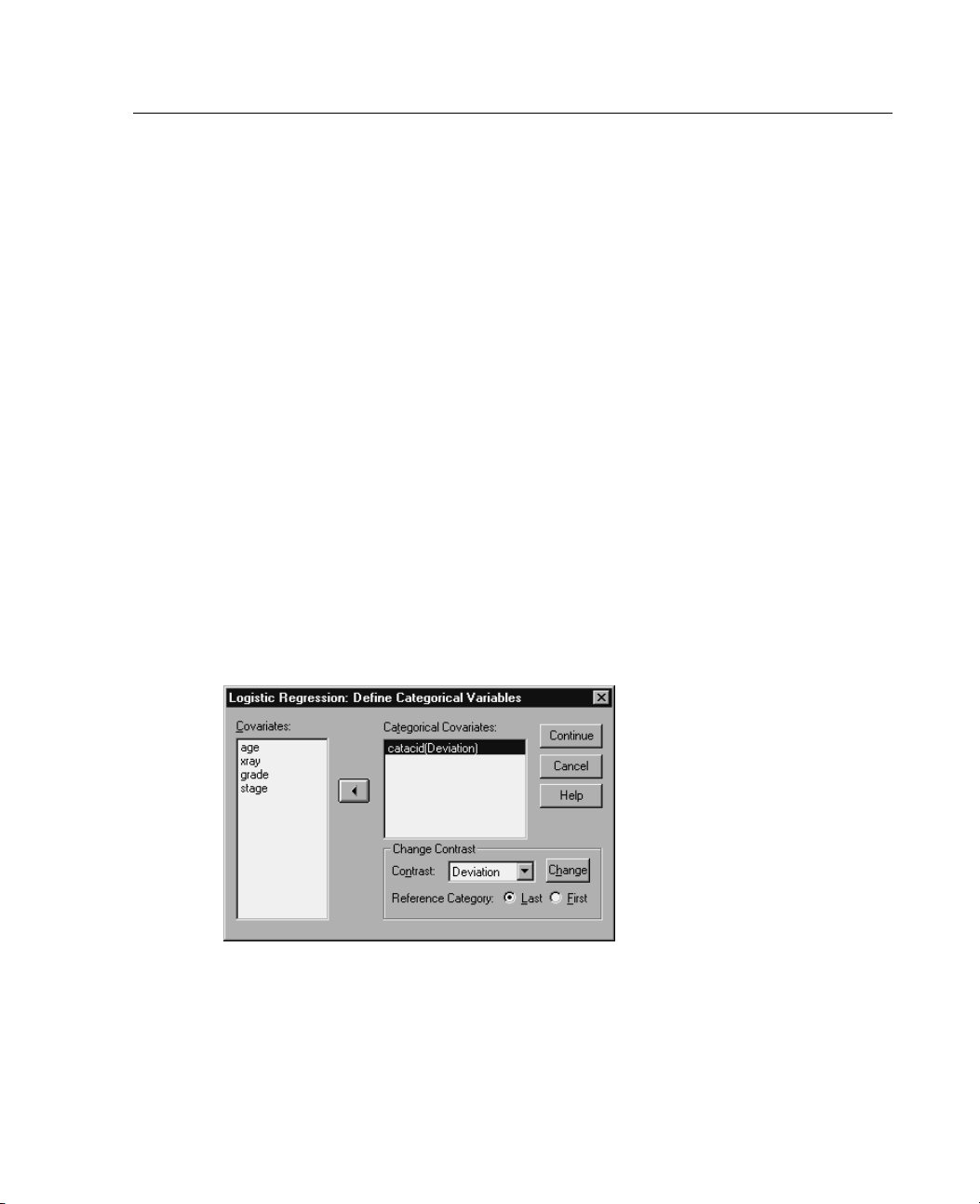
Figure 2-

Logistic

3

Regression Define Categorical Variables dialog box

Logistic Regre

ssion

8

Chapter 2

You can specify details of how the Logistic Regression procedure will handle
categorical variables:

.

Covariates

Contains a list of all of the covariates specified in the main dialog box,
either by themselves or as part of an interaction, in any layer. If some of these are
string variables or are categorical, you can use them only as categorical covariates.

Categorica

lCovariates.

Lists variables identified as categorical. Each variable
includes a notation in parentheses indicating the contrast coding to be used. String
variables (denoted by the symbol < following their names) are already present in
the Catego

rical Covariates list. Select any other categorical covariates from the

Covariates list and move them into the Categorical Covariates list.

Change Contrast. Allows you to change the contrast method. Available contrast

methods ar

 Indicato

e:

r.

Contrasts indicate the presence or absence of category membership.

The reference category is represented in the contrast matrix as a row of zeros.

 Simple. Each category of the predictor variable (except the reference category) is

compared to the reference category.

 Difference. Each category of the predictor variable except the first category is

compared

to the average effect of previous categories. Also known as reverse

Helmert contrasts.

 Helmert. Each category of the predictor variable except the last category is

compared to the average effect of subsequent categories.

 Repeated. Each category of the predictor variable except the first category is

compared

 Polynom

to the category that precedes it.

ial.

Orthogonal polynomial contrasts. Categories are assumed to be

equally spaced. Polynomial contrasts are available for numeric variables only.

 Deviation. Each category of the predictor variable except the reference category is

compared to the overall effect.

If you select Deviation, Simple,orIndicator,selecteitherFirst or Last as the reference
categor

y. Note that the method is not actually changed until you click

Change.

String covariates must be categorical covariates. To remove a string variable from
the Categorical Covariates list, you must remove all terms containing the variable
from the

Covariates list in the main dialog box.

9

Logistic Reg

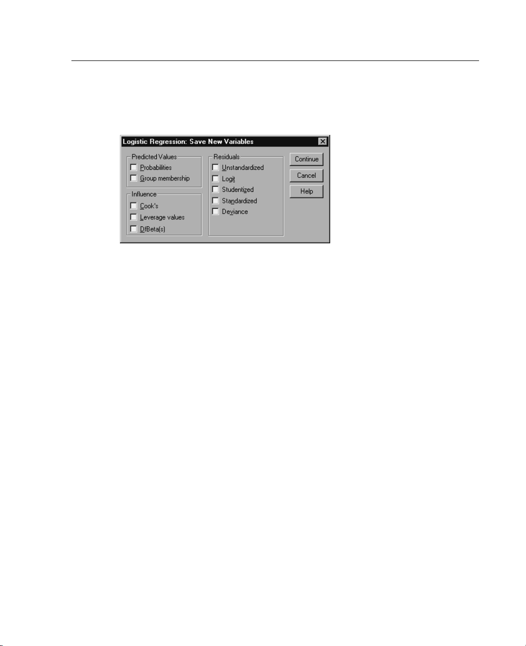
Figure 2-4

Logistic Regression Save New Variables dialog box

You can save results of the logistic regression as new variables in the working data file:

Predicted Values. Saves values predicted by the model. Available options are

Probabilities and Group membership.

 Probabilities. For each case, saves the predicted probability of occurrence of the

event. A table in the output displays name and contents of any new variables.

 Predicted Group Membership. Thegroupwiththelargestposterior probability,

based on discriminant scores. The group the model predicts the case belongs to.

ression Save New Variables

Logistic Regre

ssion

Influence. Saves values from statistics that measure the influence of cases on predicted

values. Available options are Cook's, Leverage values, and DfBeta(s).

 Cook's. The logistic regression analog of Cook's influence statistic. A measure

of how much the residuals of all cases would change if a particular case were
excluded from the calculation of the regression coefficients.

 Leverage Value. The relative influence of each observation on the model's fit.
 DfBeta(s). The difference in beta value is the change in the regression coefficient

that results from the exclusion of a particular case. A value is computed for each
term in the model, including the constant.

Residuals. Saves residuals. Available options are Unstandardized, Logit, Studentized,

Standardized, and Deviance.

 Unstandardized Residuals. The difference between an observed value and the

valuepredictedbythemodel.

10

Chapter 2



Logit Residual. The residual for the case if it is predicted in the logit scale. The

logit resid

ual is the residual divided by the predicted probability times 1 minus

the predicted probability.

 Studentized Residual. The change in the model deviance if a case is excluded.
 Standardized Resid uals. The residual divided by an estimate of its standard

deviation. Standardized residuals which are also known as Pearson residuals,
have a mean o

 Deviance.

f 0 and a standard deviation of 1.

Residuals based on the model deviance.

Logistic Regression Options

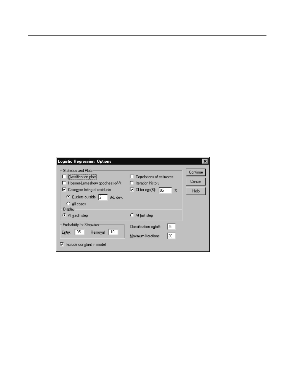
Figure 2-5

Logistic Regression Options dialog box

You can s

Statistics and Plots. Allows you to request statistics and plots. Available options

pecify options for your logistic regression analysis:

are Classification plots, Hosmer-Lemeshow goodness-of-fit, Casewise listing of

als, Correlations of estimates, Iteration history, and CI for exp(B). Select one of

residu
the alternatives in the Display group to display statistics and plots either At each step
or, only for the final model, At last step.

 Hosmer-Lemeshow goodness-of-fit statistic . This goodness-of-fit statistic is more

robust than the traditional goodness-of-fit statistic used in logistic regression,

cularly for models with continuous covariates and studies with small sample

parti

11

Logistic Regre

ssion

sizes. It is based on grouping cases into deciles of risk and comparing the
observed pr

Probability for Stepwis e. Allows you to control the criteria by which variables are

obability with the expected probability within each decile.

entered into and removed from the equation. You can specify criteria for Entry or
Removal of v

 Probabili

ariables.

ty for St epwise.

A variable is entered into the model if the probability of
its score statistic is less than the Entry value, and i s removed if the probability is
greater than the Removal value. To override the default settings, enter positive
values for

Classification cutoff. Allows you to determine the cut point for classifying cases.

Entry and Removal. Entry must be less than Removal.

Cases with predicted values that exceed the classification cutoff are classified as
positive,

while those with predicted values smaller than the cutoff are classified as

negative. To change the default, enter a value between 0.01 and 0.99.

Maximum Iterations. Allows you to change the maximum number of times that the

model ite

Include constant in model. Allows you to indicate whether the model should include a

rates before terminating.

constant term. If disabled, the constant term will equal 0.

LOGISTIC REGRESSION Command Additional Features

The SPSS command language also allows you to:

 Identify casewise output by the values or variable labels of a variable.
 Control the spacing of iteration reports. Rather than printing parameter estimates

after eve

 Change t
 Specify
 Conserv

scratch file during processing.

ry iteration, you can request parameter estimates after every nth iteration.

he criteria for terminating iteration and checking for redundancy.
a variable list for casewise listings.
e memory by holding the data for each split file group in an external

Chapter

3

Multinomial

Multinomial Logistic Regression is useful for situations in which you want to be
able to clas
of regression is similar to logistic regression, but it is more general because the
dependent variable is not restricted to two categories.

Example. I

what type of film a moviegoer is likely to see. By performing a Multinomial Logistic
Regression, the studio can determine the strength of influence a person's age, gender,
and datin
advertising campaign of a particular movie toward a group of people likely to go see it.

Statistics. Iteration history, parameter coefficients, asymptotic covariance and

correlat
log-likelihood. Pearson and deviance chi-square goodness of fit. Cox and Snell,
Nagelkerke, and McFadden R
by respo
residuals) and proportions by covariate pattern and response category.

sify subjects based on values of a set of predictor variables. This type

n order to market films more effectively, movie studios want to predict

g status has upon the type of film they prefer. The studio can then slant the

ion matrices, likelihood-ratio tests for model and partial effects, –2

nse category. Crosstabulation: observed and predicted frequencies (with

Logistic Regression

2

. Classification: observed versus predicted frequencies

Multin

Methods. A multinomial logit model is fit for the full factorial model or a

user-sp
maximum-likelihood algorithm.

ecified model. Parameter estimation is performed through an iterative

omial Logistic Regression Data Considerations

Data. T

factors or covariates. In general, factors should be categorical variables and covariates
should be continuous variables.

he dependent variable should be categorical. Independent variables can be

13

14

Chapter 3

Assumptions. It is assumed that the odds ratio of any two categories are independent

of all other response categories. For example, if a new product is introduced to a
market, thi

s assumption states that the market shares of all other products are affected
proportionally equally. Also, given a covariate pattern, the responses are assumed to
be independent multinomial variables.

Obtaining a Multinom ial Logistic Regression

E From the menus choose:

Analyze

Regression

Multinomial Logistic...

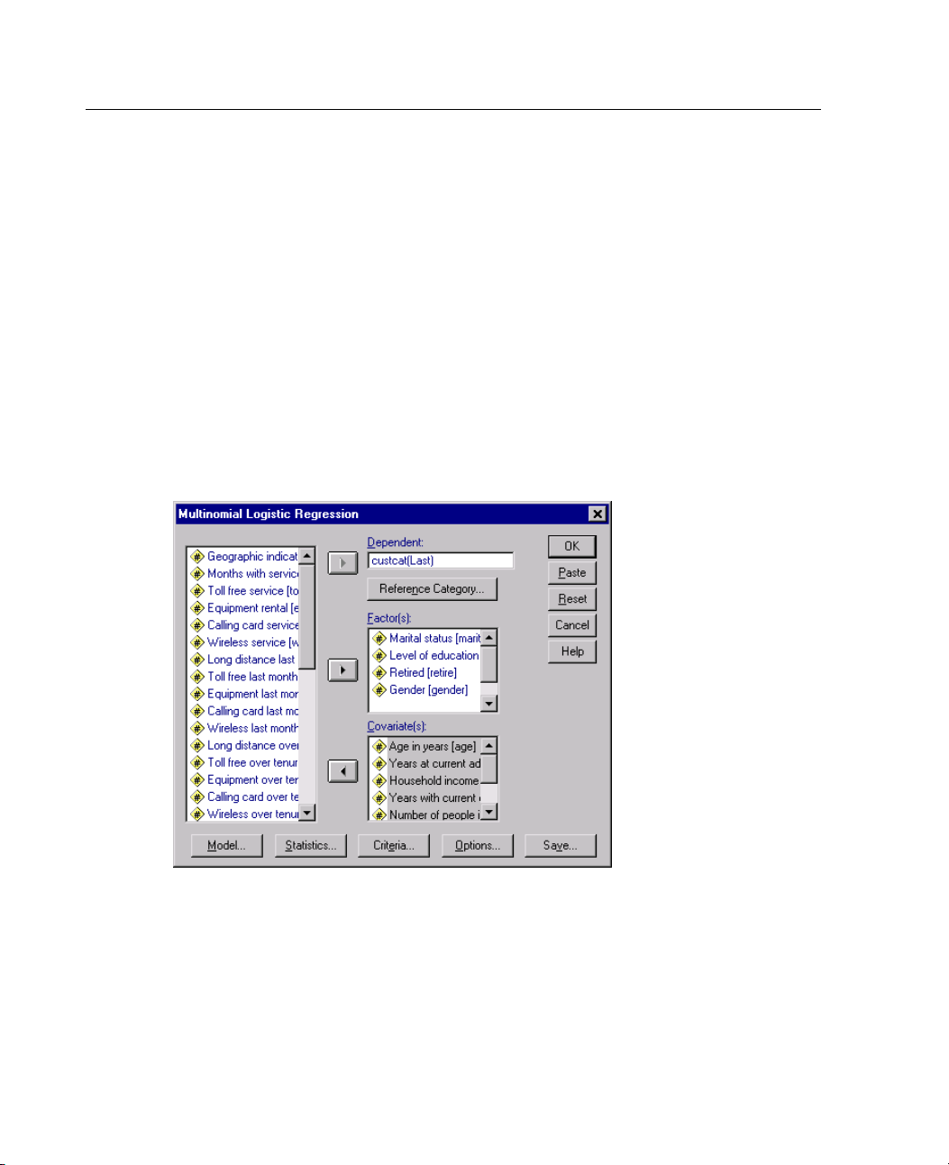
Figure 3-1

Multinomial Logistic Regression dialog box

E Select one dependent variable.
E Factors are optional and can be either numeric or categorical.
E Covariates are optional but must be numeric if specified.

15

Multinomial

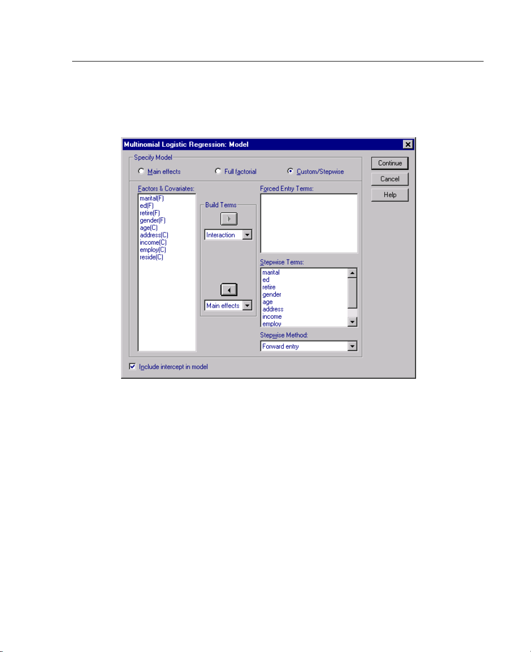
Figure 3-2

Multinomial Logistic Regression Model dialo g box

Logistic Regression Models

Multinomial Lo

gistic Regression

By default, the Multinomial Logistic Regression procedure produces a model with
the factor and covariate main effects, but you can specify a custom model or request
stepwise model selection with this d ialog box.

Specify Model. A main-effects model contains the covariate and factor main effects

but no interaction effects. A full factorial model contains all main effects and all
factor-by-factor interactions. It does not contain covariate interactions. Youcan create
a custom model to specify subsets of factor interactions or covariate interactions, or
request stepwise selection of model terms.

Factors and Covariates. The factors and covariates are listed with (F) for factor and

(C) for covariate.

Forced Entry Terms. Terms added to the forced entry list are always included in the

model.

16

Chapter 3

Stepwise Terms. Terms added to the stepwise list are included in the model according

to one of the following user-selected methods:

 Forward entry. This method begins with no stepwise terms in the model. At each

step, the most significant term is added to the model until none of the stepwise
terms left o

ut of the model would have a statistically significant contribution if

addedtothemodel.

 Backward elimination. This method begins by entering all terms specified on the

stepwise list into the model. At each step, the least significant stepwise term
is removed

from the model until all of the remaining stepwise terms have a

statistically significant contribution to the model.

 Forward stepwise. This method begins with the model that would be selected by

the forward entry method. From there, the algorithm alternates between backward
eliminati

on on the stepwise terms in the model and forward entry on the terms left

out of the model. This continues until no terms meet the entry or removal criteria.

 Backward stepwise. This method begins with the model that would be selected by

the b ackward elimination method. From there, the algorithm alternates between
forward e

ntry on the terms left out of the model and backward elimination on
the stepwise terms in the model. This continues until no terms meet the e ntry or
removal criteria.

Include intercept in model. Allows you to include or exclude an intercept term for the

model.

Build Terms

For the selected factors and covariates:

Interac

Main effects. Creates a main-effects term for each variable selected.
All 2-way. Creates all possible two-way interactions of the selected variables.

All 3-wa

All 4-way. Creates all possible four-way interactions of the selected variables.
All 5-way. Creates all possible five-way interactions of the selected variables.

tion.

Creates the highest-level interaction term of all selected variables.

y.

Creates all possible three-way interactions of the selected variables.

17

Multinomial

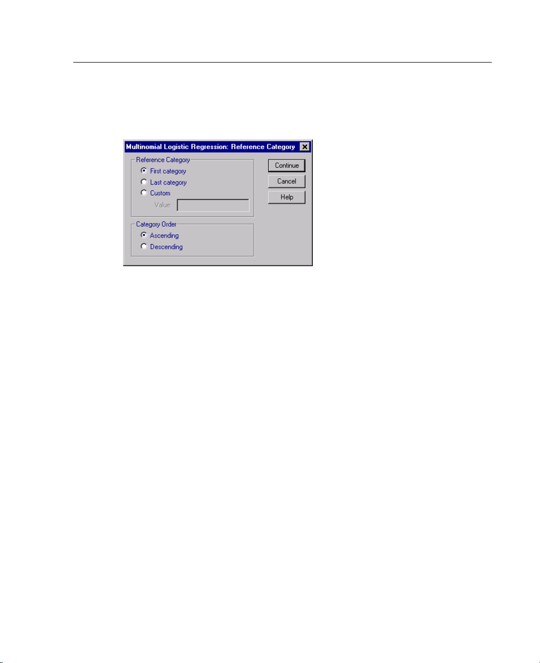
Figure 3-3

Multinomial Logistic Regression Reference Category dialog box

By default, the M ultinomial Logistic Regression procedure makes the last category
the reference category. This dialog box gives you control of the reference category
and the way in which categories are ordered.

Reference Category. Specify the first, last, or a custom category.
Category Order. In ascending order, the lowest value defines the first category and the

highest value defines the last. In descending order, the highest value defines the first
category and the lowest value defines the last.

Multinomial Lo

Logistic Regression Reference Category

gistic Regression

18

Chapter 3

Multinomial

Figure 3-4

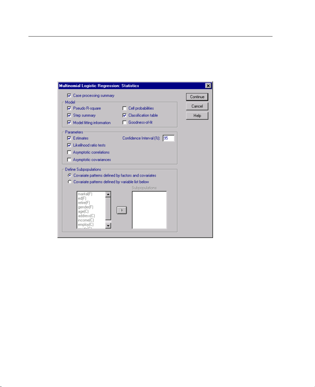
Multinomial Logistic Regression Statistics dialog box

Logistic Regression Statistics

You can specify the following statistics for your Multinomial Logistic Regression:

Case pro cessing summary. This table contains information about the specified

categorical variables.

Model. Statistics for the overall model.

 Summary statistics. Prints the Cox and Snell, Nagelkerke, and McFadden R

2

statistics.

 Step summary. This table summarizes the effects entered or removed at each step

in a stepwise method. It is not produced unless a stepwise model is specified in
the Model dialog box.

 Model fitting information. This table compares the fitted and intercept-only

or null models.

19

Multinomial Lo



Cell probabilities. Prints a table of the observed and expected frequencies (with

residual) a

 Classifica

 Goodness of

nd proportions by covariate pattern and response category.

tion table.

fit chi-square statistics.

Prints a table of the observed versus predicted responses.

Prints Pearson and likelihood-ratio chi-square

gistic Regression

statistics. Statistics are computed for the covariate patterns determined by all
factors and covariates or by a user-defined subset of the factors and covariates.

Parameters. Statistics related to the model parameters.

 Estimates. Prints estimates of the model parameters, with a user-specified level of

confidence.

 Likelihood ratio test. Prints likelihood-ratio tests for the model partial effects. The

test for the

 Asymptoti

 Asymptoti

Define Subp

overall model is printed automatically.

c correlations.

c covariances.

opulations.

Prints matrix of parameter estimate correlations.
Prints matrix of parameter estimate covariances.

Allows you to select a subset of the factors and covariates in
order to define the covariate patterns used by cell probabilities and the goodness-of-fit
tests.

Multinomial Logistic Regression Criteria

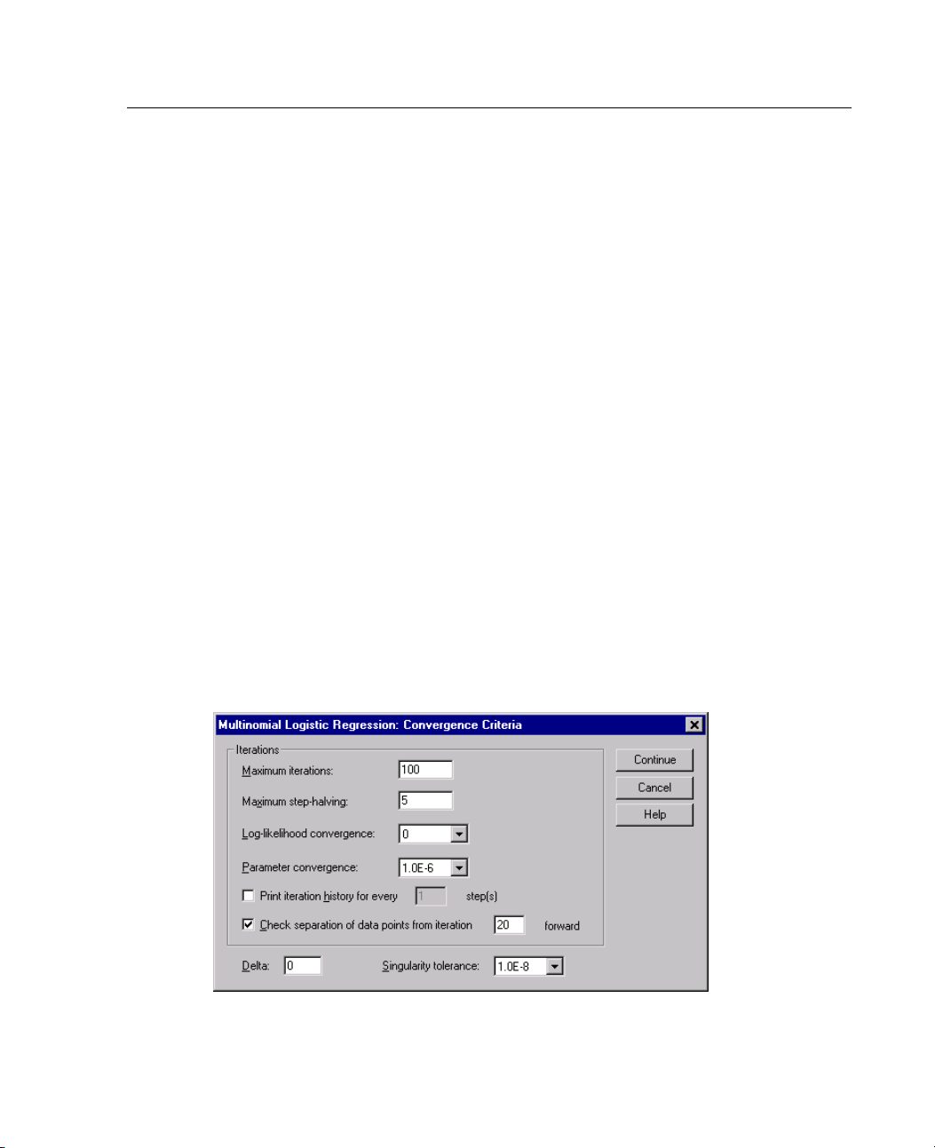
Figure 3-5

Multinomi

al Logistic Regression Convergence Criteria dialog box

20

Chapter 3

You can specify the following criteria for your Multinomial Logistic Regression:

Iterations. Allows you to specify the maximum number of times you want to cycle

through the

algorithm, the maximum number of steps in the step-halving, the
convergence tolerances for changes in the log-likelihood and parameters, how often
the progress of the iterative algorithm is printed, and at what iteration the procedure
should begi

 Log-likel

n checking for complete or quasi-complete separation of the data.

ihood Convergence.

Convergenceisassumediftherelativechangein
the log-likelihood function is less thanthespecifiedvalue. Thevaluemust
be positive.

 Parameter Convergenc e. The algorithm is assumed to have reach the c orrect

estimates

if the absolute change or relative change in the parameter estimates is

less than this value. The criterion is not used if the value is 0.

Delta. All

ows you to specify a non-negative value less than 1. This value is added to
each empty cell of the crosstabulation of response category by covariate pattern. This
helps to stabilize the algorithm and prevent bias in the estimates.

Singular

ity tole rance.

Allows you to specify the tolerance used in checking for

singularities.

21

Multinomial

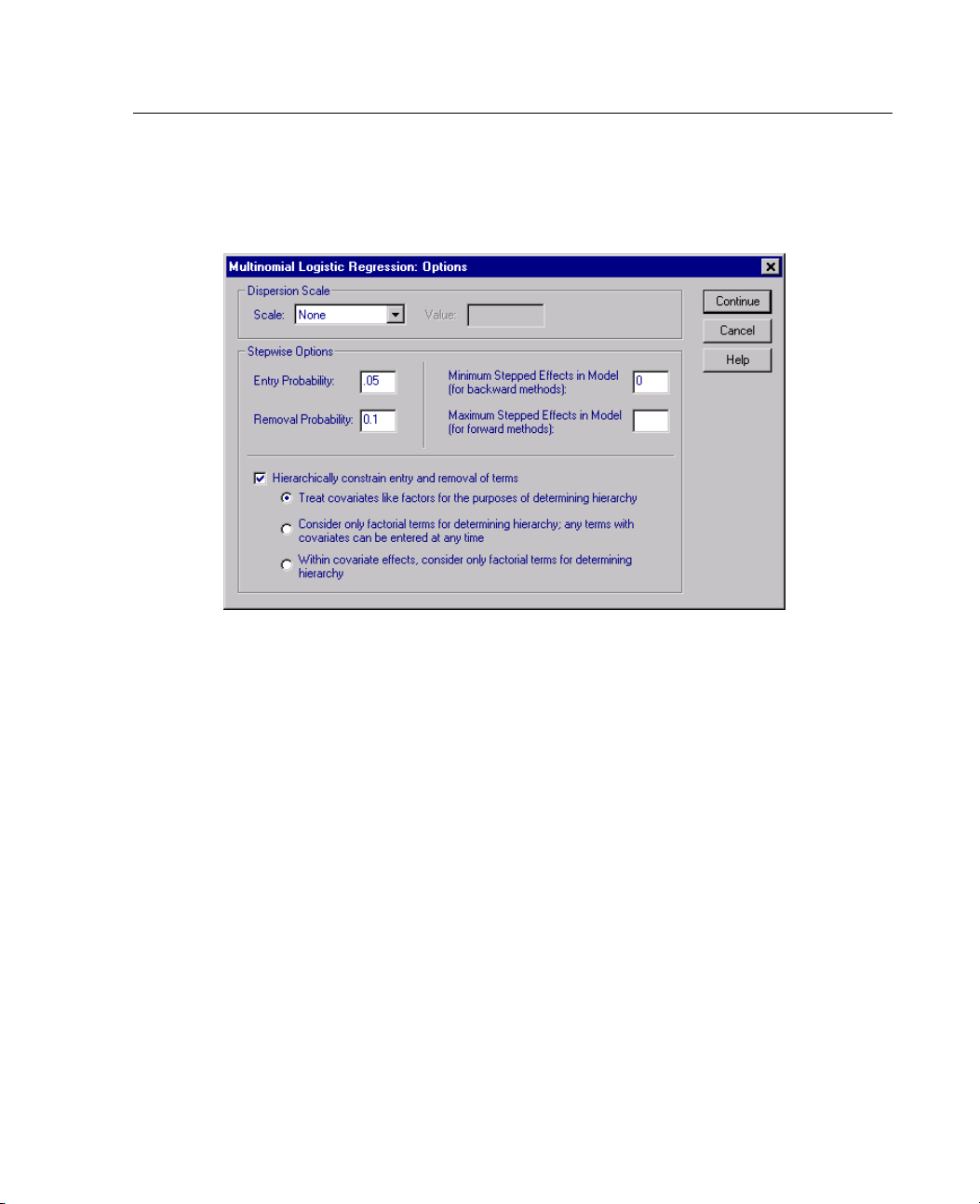
Figure 3-6

Multinomial Logistic Regression Options dialog box

You can specify the following options for your Multinomial Logistic Regression:

Logistic Regression Options

Multinomial Lo

gistic Regression

Dispersion Scale. Allows you to specify the dispersion scaling value that will be

used to

correct t he estimate of the parameter covariance matrix.

Deviance estimates

the scaling value using the deviance function (likelihood-ratio chi-square) statistic.

Pearson estimates the scaling value using the Pearson chi-square statistic. You can

pecify your own scaling value. It must be a positive numeric value.

also s

Stepwise Options. These options give you control of the statistical criteria when

stepwise methods are used to build a model. They are ignored unless a stepwise

is specified in the Model dialog box.

model

 Entr

y Probability.

This is the probability of the likelihood-ratio statistic for variable
entry. The larger the specified probability, t he easier it is for a variable to enter
the model. This criterion is ignored unless the forward entry, forward stepwise,

ckward stepwise method is selected.

or ba

22

Chapter 3



Removal Probability. This is the probability of the likelihood-ratio statistic for

variable re

moval. The larger the specified probability, the easier it is for a variable
to remain in the model. This criterion is ignored unless the backward elimination,
forward stepwise, or backward stepwise method is selected.

 Minimum Stepped Effe ct in Model. When using the backward elimination or

backward st

epwise methods, this specifies the minimum number of terms to

include in the model. The intercept is not counted as a model term.

 Maximum S tep ped Effect in Model. When using the forward entry or forward

stepwise methods, this specifies the maximum number of terms to include in the
model. The

 Hierarch

intercept is not counted as a model term.

ically constrain entry and removal of terms.

This option allows you to
choose whether to place restrictions on the inclusion of model terms. Hierarchy
requires that for any term to be included, all lower order terms that are a part of
the term t

o be included must be in the model first. For example, if the hierarchy
requirement is in effect, the factors Marital status and Gender must both be in the
model before the Marital Status*Gender interaction can be added. The three
radio but

ton options determine the role of covariates in determining hierarchy.

Multinomial Logistic Regression Save

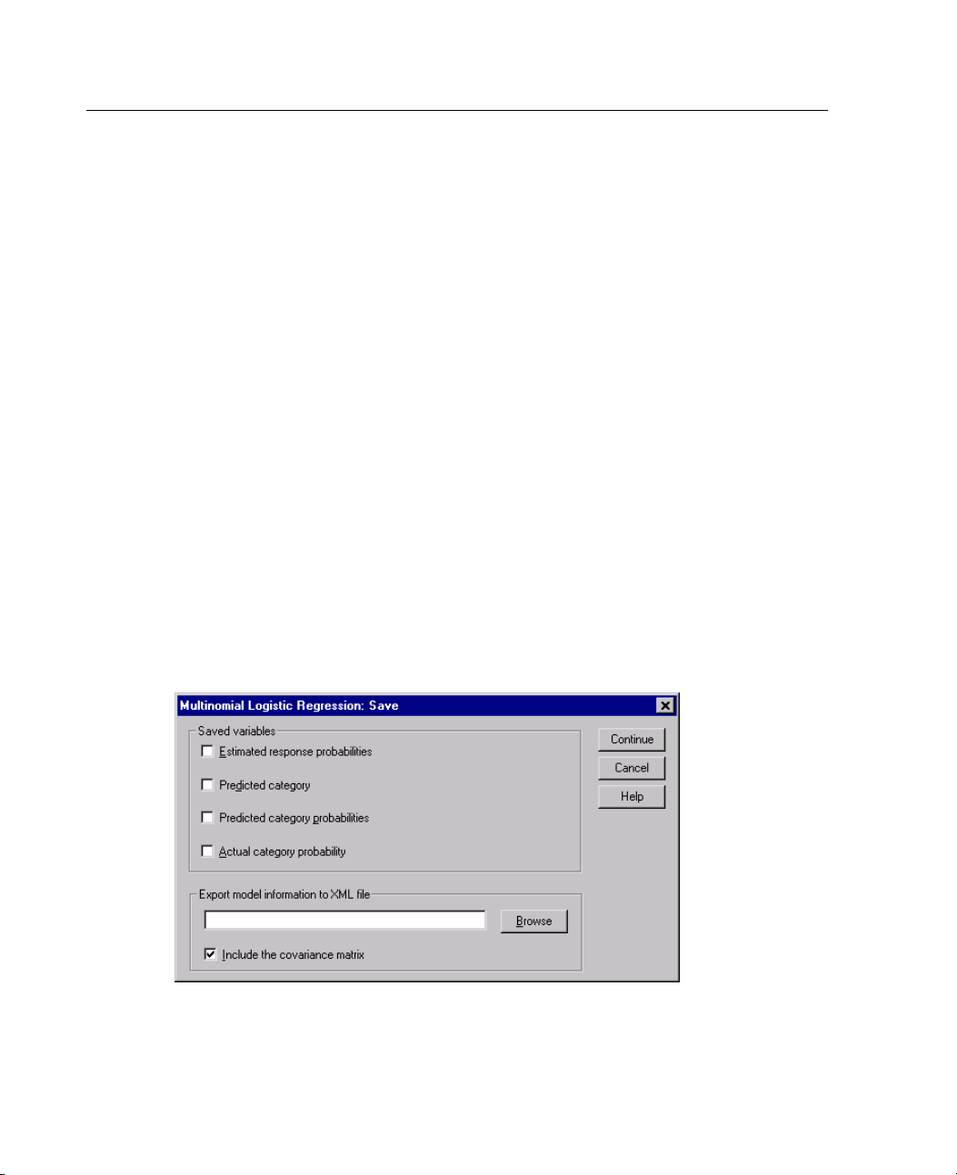
Figure 3-7

Multinomial Logistic Regression Save dialog box

23

The Save dialog box allows you to save variables to the working file and export
model information to an external file.

Saved varia

 Estimated r

bles.

esponse probabilities.

These are the estimated probabilities of
classifying a factor/covariate pattern into the response categories. There are as
many estimated probabilities as there are categories of the response variable; up
to 25 will be

 Predicted

saved.

category.

This is the response category with the largest expected

probability for a factor/covariate pattern.

 Predicted cate gor y probabilities. This is the maximum of the estimated response

probabilities.

 Actual category probability. This is the estimated probability of classifying a

factor/co

Export mod

variate pattern into the observed category.

el information to XML file.

Parameter estimates and (optionally) their
covariances are exported to the specified file. SmartScore and future releases of
WhatIf? will be able to use this file.

NOMREG Command Additional Features

Multinomial Lo

gistic Regression

The SPSS command language also allows you to:

 Specify the reference category of the dependent variable.
 Include cases with user-missing values.
 Customize hypothesis tests by specifying null hypotheses as linear combinations

of parame

ters.

Chapter

4

Probit Analy

This procedure measures the relationship between the strength of a stimulus and the
proportion
situations where you have a dichotomous output that is thought to be influenced or
caused by levels of some independent variable(s) and is particularly well suited to
experimen
required to induce a certain proportion of responses, such as the median effective dose.

Example. How effective is a new pesticide at killing ants, and what is an appropriate

concentr
of ants to different concentrations of the pesticide and then record the number of ants
killed and the number of ants exposed. Applying probit analysis to these data, you
can deter
you can determine what the appropriate concentration of pesticide would be if you
wanted to be sure to kill, say, 95% of exposed ants.

Statist

error, Pearson goodness-of-fit chi-square, observed and expected frequencies, and
confidence intervals for effective levels of independent variable(s). Plots: transformed
respon

of cases exhibiting a certain response to the stimulus. It is useful for

tal data. This procedure will allow you to estimate the strength of a stimulus

ation to use? You might perform an experiment in which you expose samples

mine the strength of the relationship between concentration and killing, and

ics.

Regression coefficients and standard errors, intercept and standard

se plots.

sis

Probit

®

This pr
Murray, Saunders & Wright to estimate the model parameters.

ocedure uses the algorithms proposed and implemented in NPSOL

by Gill,

Analysis Data Considerations

or each value of the independent variable (or each combination of values for

Data. F

multiple independent variables), your response variable should be a count of the
number of cases with those values that show the response of interest, and the total

25

26

Chapter 4

observed variable should be a count of the total number of cases with those values for
the independent variable. The factor variable should be categorical, coded as integers.

s.

Assumption

Observations should be independent. If you have a large number of
values for the independent variables relative to the number of observations, as you
might in an observational study, the chi-square and goodness-of-fit statistics may
not be valid

Related procedu res. Probit analysis is closely related to logistic regression; in fact, if

.

you choose the logit transformation, this procedure will essentially compute a logistic
regressio

n. In general, probit analysis is appropriate for designed experiments,
whereas logistic regression is more appropriate for observational studies. The
differences in output reflect these different emphases. The probit analysis procedure
reports e

stimates of effective values for various rates of response (including median
effective dose), while the logistic regression procedure reports estimates of odds
ratios for independent variables.

Obtaining a Probit A nalysis

E From the menus choose:

Analyze

Regression

Probit...

27

Probit Analysi

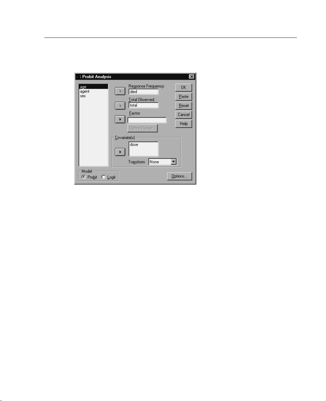
Figure 4-1

Probit Analysis dialog box

E Select a response frequency variable. This variable indicates the number of cases

exhibiting a response to the test stimulus. The values of this variable cannot be
negative.

s

E Select a total observed variable. This variable indicates the number of cases to which

the stimulus was applied. The values of this variable cannot be negative and cannot
be less than the values of the response frequency variable for each case.

Optionally, you can select a Factor variable. If you do, click

Define Range to define

the groups.

E Select one or more covariate(s). This variable contains the level of the stimulus

applied to each observation. If you want to transform the covariate, select a
transformation from the Transform drop-down list. If no transformation is applied
and there is a control group, then the control group is included in the analysis.

E Select either the Probit or Logit model.

 Probit Model. Applies the probit transformation (the inverse of the cumulative

standard normal distribution function) to the response proportions.

 Logit Model. Applies the logit (log odds) transformation to the response

proportions.

28

Chapter 4

Probit Analy

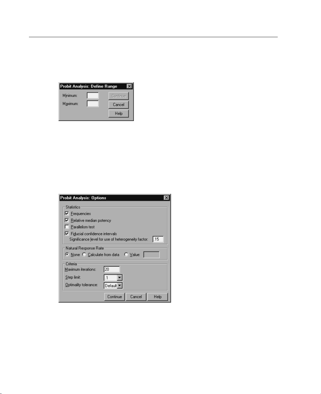
Figure 4-2

Probit Analysis Define Range dialog box

This allows you to specify the levels of the factor variable that will be analyzed. The
factor levels must be coded as consecutive integers, and all levels in the range that
you specify will be analyzed.

sis Define Range

Probit Analysis Options

Figure 4-

Probit An

3

alysis Options dialog box

You can specify options for your probit analysis:

Statistics. Allows you to request the following optional statistics: Frequencies,

ive median potency, Parallelism test, and Fiducial confidence intervals.

Relat

29

Probit Analysi



Relative Median Potency. Displays the ratio of median potencies for each pair

of factor le

vels. Also shows 95% confidence limits for each relative median
potency. Relative median potencies are not available if you do not have a factor
variable or if you have more than one covariate.

 Parallelism Test. A test of the hypothesis that all factor levels have a common

slope.

 Fiducial C

onfidence In tervals.

Confidence intervals for the dosage of agent

required to produce a certain probability of response.

Fiducial co

nfidence intervals and Relative median potency are unavailable if you have
selected more than one covariate. Relative median potency and Parallelism test are
available only if you have selected a factor variable.

Natural Re

sponse Rate.

Allows you to indicate a natural response rate even in the
absence of the stimulus. Available alternatives are None, Calculate from data,
or Value.

 Calculate from Data. Estimate the natural response rate from the sample data.

Your data should contain a case representing the control level, for which the
value of t

he covariate(s) is 0. Probit estimates the natural response rate using the

proportion of responses for the control level as an initial value.

 Value. Sets the natural response rate in the model (select this item when you know

the natural response rate in advance). Enter the natural response proportion (the
proporti

on must be less than 1). For example, if the response occurs 10% of the

time when the stimulus is 0, enter 0.10.

s

a.

Criteri

Allows you to control parameters of the iterative parameter-estimation
algorithm. You can override the defaults for Maximum iterations, Step limit, and
Optimality tolerance.

PROBIT Command Additional Features

The SPSS command language also allows you to:

 Request an analysis on both the probit and logit models.
 Control the treatment of missing values.
 Transform the covariates by bases other than base 10 or natural log.

Chapter

5

Nonlinear Re

Nonlinear regression is a method of finding a nonlinear model of the relationship
between the
linear regression, which is restricted to estimating linear models, nonlinear regression
can estimate models with arbitrary relationships between independent and dependent
variables
procedure is not necessary for simple polynomial models of the form Y = A + BX**2.
By defining W = X**2, we get a simple linear model, Y = A + BW, which can be
estimate

Example. Can population be predicted based on time? A scatterplot shows that there

seems to be a strong relationship between population and time, but the relationship is
nonlinea
procedure. By setting up an appropriate equation, such as a logistic population growth
model, we can get a good estimate of the model, allowing us to make predictions
about po

Statistics. For each iteration: parameter estimates and residual sum of squares. For

each model: sum of squares for regression, residual, uncorrected total and corrected
total,
matrix of parameter estimates.

dependent variable and a set of independent variables. Unlike traditional

. This is accomplished using iterative estimation algorithms. Note that this

d using traditional methods such as the Linear Regression procedure.

r, so it requires the special estimation methods of the Nonlinear Regression

pulation for times that were not actually measured.

parameter estimates, asymptotic standard errors, and asymptotic correlation

gression

Note: Constrained nonlinear regression uses the algorithms proposed and

®

implemented in NPSOL
model p

arameters.

by Gill, Murray, Saunders, and Wright to estimate the

31

32

Chapter 5

Nonlinear Re

Data. The de

variables, such as religion, major, or region of residence, need to be recoded to binary
(dummy) variables or other types of contrast variables.

Assumption

describes the relationship between dependent and independent variables.
Additionally, the choice of good starting values is very important. Even if you've
specified
your model may fail to converge or you may get a locally optimal solution rather
than one that is globally optimal.

Related pr

a linear model, which can be analyzed using the Linear Regression procedure. If you
are uncertain what the proper model should be, the Curve Estimation procedure can
help to id

gression Data Considerations

pendent and independent variables should be quantitative. Categorical

s.

Results a re valid only if you have specified a function that accurately

the correct functional form of the model, if you use poor starting values,

ocedures.

entify useful functional relations in your data.

Many models that appear nonlinear at first can be transformed to

Obtaining a Nonlinear Regression Analysis

E From the menus choose:

Analyze

Regressi

Nonlinea

on

r...

33

Nonlinear Regr

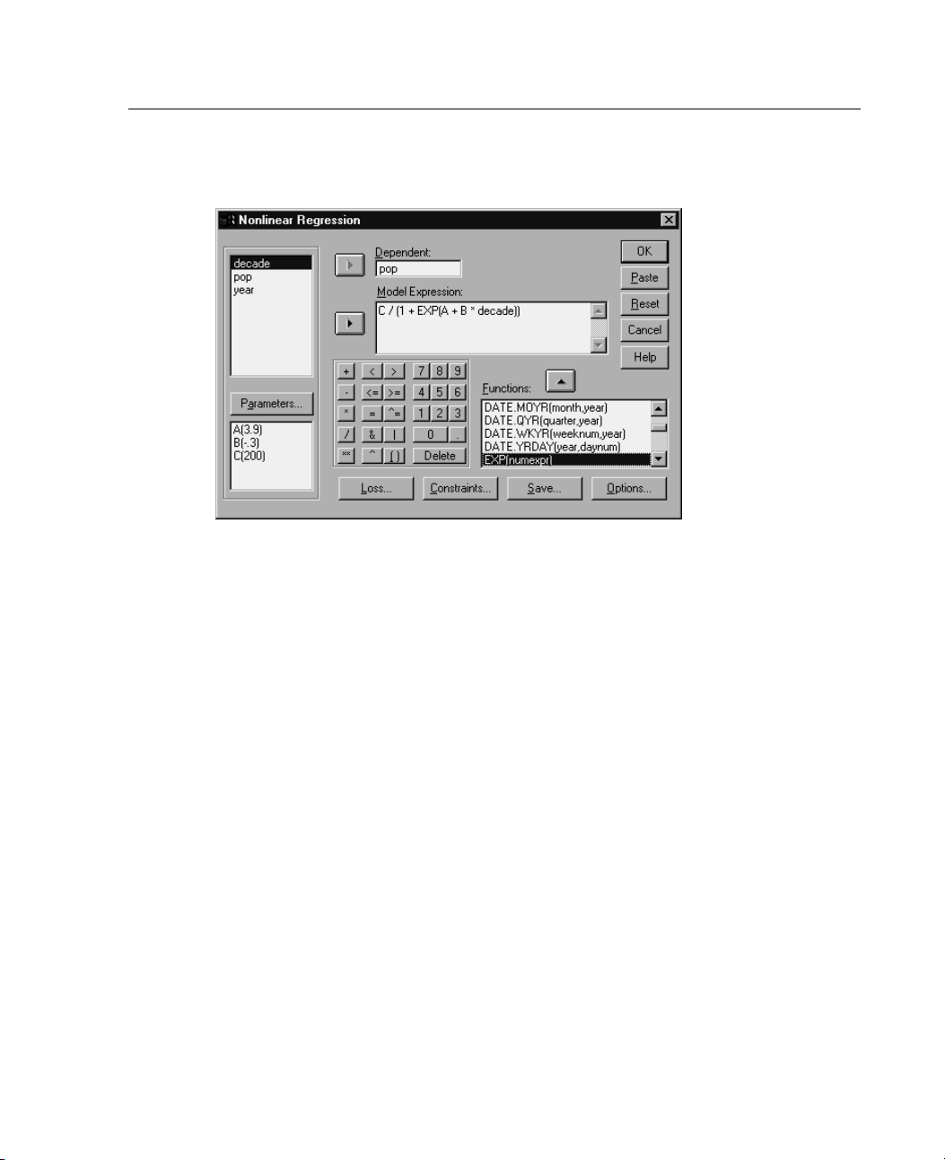
Figure 5-1

Nonlinear Regression dialog box

E Select

one numeric dependent variable from the list of variables in your working

data file.

E To build a model expression, enter the expression in the Model field or paste

components (variables, parameters, functions) into the field.

ession

Condit

E Identify parameters in your model by clicking Parameters.

Asegmen

ted model (one that takes different forms in different parts of its domain)

must be specified by using conditional logic within the single model statement.

ional Logic (Nonlinear Regression)

You can
within a model expression or a loss function, you form the sum of a series of terms,
one for each condition. Each term consists of a logical expression (in parentheses)
multip

For example, consider a segmented model that equals 0 for X<=0, X for 0<X<1, and
1 for X>=1. The expression for this is:

(X<=0)

specify a segmented model using conditional logic. To use conditional logic

lied by the expression that should result when that logical expression is true.

*0 + (X>0 & X < 1)*X + (X>=1)*1.

34

Chapter 5

The logical expressions in parentheses all evaluate to 1 (true) or 0 (false). Therefore:
If X<=0, the above reduces to 1*0 + 0*X + 0*1=0.
If 0<X<1, it r

educes to 0*0 + 1*X +0*1 = X.
If X>=1, it reduces to 0*0 + 0*X + 1*1 = 1.
More complicated examples can be easily built by substituting different logical

expression

s and outcome expressions. Remember that double inequalities, such as

0<X<1, must be written as compound expressions, such as (X>0 & X < 1).
String variables can be used within logical expressions:
(city='New

York')*costliv + (city='Des Moines')*0.59*costliv

This yields one expression (the value of the variable costliv) for New Yorkers and
another (59% of that value) for Des Moines residents. String constants must be
enclosed in

quotation marks or apostrophes, as shown here.

Nonlinear Regression Parameters

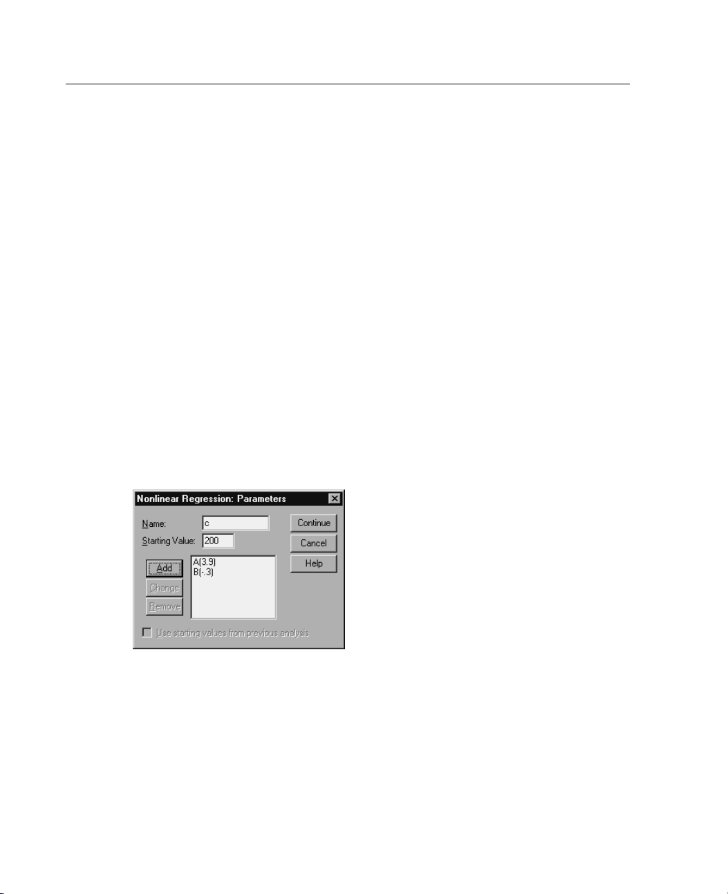
Figure 5-2

Nonlinear Regression Parameters dialog box

Parameters are the parts of your model that the Nonlinear Regression procedure
estimates. Parameters can be additive constants, multiplicative coefficients,
exponen

ts, or values used in evaluating functions. All parameters that you have
defined will appear (with their initial values) on the Parameters list in the main
dialog box.

35

Name. You must specify a name for each parameter. This name must be a valid

SPSS variable name and must be the name used in the model expression in the main
dialog box.

Starting Value. Allows you to specify a starting value for the parameter, preferably

as close as possible to the expected final solution. Poor starting values can result in
failure to c

onverg e or in convergence on a solution that is local (rather than global) or

is physically impossible.

Use starting values from previous analysis. If you have already run a nonlinear

regressio

n from this dialog box, you can select this option to obtain the initial values
of parameters from their values in the previous run. This permits you to continue
searching when the algorithm is converging slowly. (The initial starting values will
still app

ear on the Parameters list in the main dialog box.)

Note: This selection persists in this dialog box for the rest of your session. If you
change the model, be sure to deselect it.

Nonlinear Regression Common Models

The table below provides example model syntax for many published nonlinear
regression models. A model selected at random is n ot likely to fit your data well.
Appropr
constraints in order to converge.

Tab l e 5- 1

Example model syntax

Name Model ex

AsymptoticRegression b1+b2*exp(b3*x)
Asymptotic Regression b1 –( b2 *( b3 ** x ))
Density ( b1 + b2 * x )**(–1/ b3 )
Gauss b1 *(1– b3 *exp( –b2 * x **2))
Gompertz b1 *exp( –b2 * exp( –b3 * x ))
Johnson-Schumacher b1 *exp( –b2 / ( x + b3))
Log-Modified (b1+b3*x)**b2
Log-Logistic b1 –ln (1+ b2 *exp( –b3 * x ))

iate starting values for the parameters are necessary, and some models require

pression

Nonlinear Regr

ession

36

Chapter 5

Name Model expression

Metcherlich Law of Diminishing
Returns

MichaelisMenten b1*x/(x+b2)
Morgan-Mercer-Florin (b1*b2+b3*x**b4)/(b2+x**b4)
Peal-Reed
Ratio of Cubics
RatioofQuadratics (b1+b2*x+b3*x**2)/(b4*x**2)
Richards b1 /((1+ b3 *exp(– b2 * x ))**(1/ b4 ))
Verhulst b1/(1+b3*exp(–b2*x))
VonBertalanffy (b1**(1–b4)–b2*exp(–b3*x))**(1/(1–b4))
Weibull b1–b2*exp(–b3*x**b4)
Yield Density (b1 + b2 * x + b3 * x **2)**(–1)

b1+b2*exp(–b3*x)

b1 /(1+ b2 *exp(–( b3 * x + b4 * x **2+ b5 * x **3)))
( b1 + b2 * x + b3 * x **2+ b4 * x **3)/( b5 * x **3)

Nonlinear Regression Loss Function

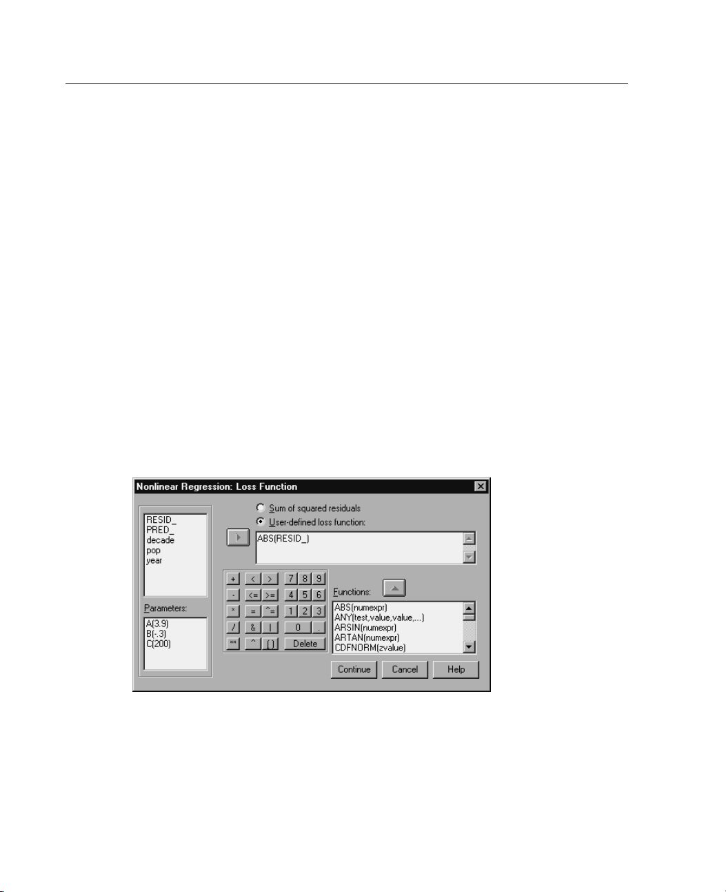
Figure 5-3

Nonlinear Regression Loss Function dialog box

The loss function in nonlinear regression is the function that is minimized by the
algorithm. Select either

Sum of squared residuals to minimize the sum of the squared

residuals or User-defined loss function to minimize a different function.

37

If you select User-defined loss function, you must define the loss function whose sum
(across all cases) should be minimized by the choice of parameter values.

 Most loss functions involve the special variable RESID_, which represents the

residual. (The default Sum of squared residuals loss function could be entered

RESID_**2.)Ifyouneedtousethepredictedvalueinyourloss

explicitly

as

function, it is equal to the dependent variable minus the residual.

 It is possible to specify a conditional loss function using conditional logic.

You can eith

er type an expression in the User-defined loss function field or paste
components of the expression into the field. String constants must be enclosed in
quotation marks or apostrophes, and numeric constants must be typed in American
format, wi

th the dot as a decimal delimiter.

Nonlinear Regression Param eter Constraints

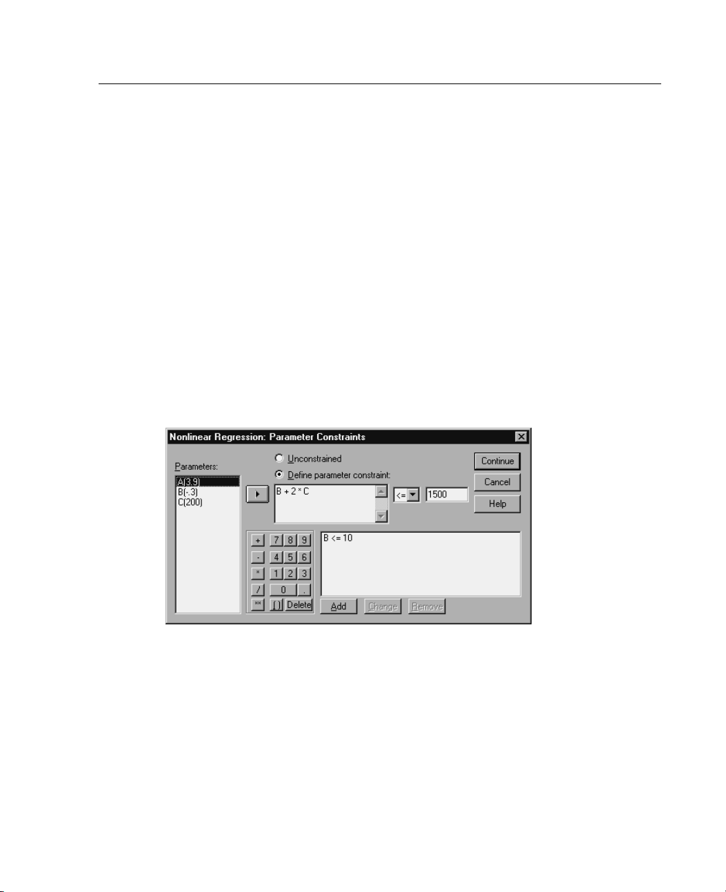
Figure 5-4

Nonlinear Regression Parameter Constraints dialog box

Nonlinear Regr

ession

A constraint is a restriction on the allowable values for a parameter during the

ive search for a solution. Linear expressions are evaluated before a step is taken,

iterat
so you can use linear constraints to prevent steps that might result in overflows.
Nonlinear expressions are evaluated after a step is taken.

38

Chapter 5

Each equation or inequality requires the following elements:

 An expression involving at least one parameter in the model. Type the expression

or use the key

pad, which allows you to paste numbers, operators, or parentheses

into the expression. You can either type in the required parameter(s) along with
the rest of the expression or paste from the Parameters list at the left. You cannot
use ordinar

 One of the t
 Anumericc

y variables in a constraint.

hree logical operators <=, =, or >=.

onstant, to which the expression is compared using the logical
operator. Type the constant. Numeric constants must be typed in American
format, with the dot as a decimal delimiter.

Nonlinear

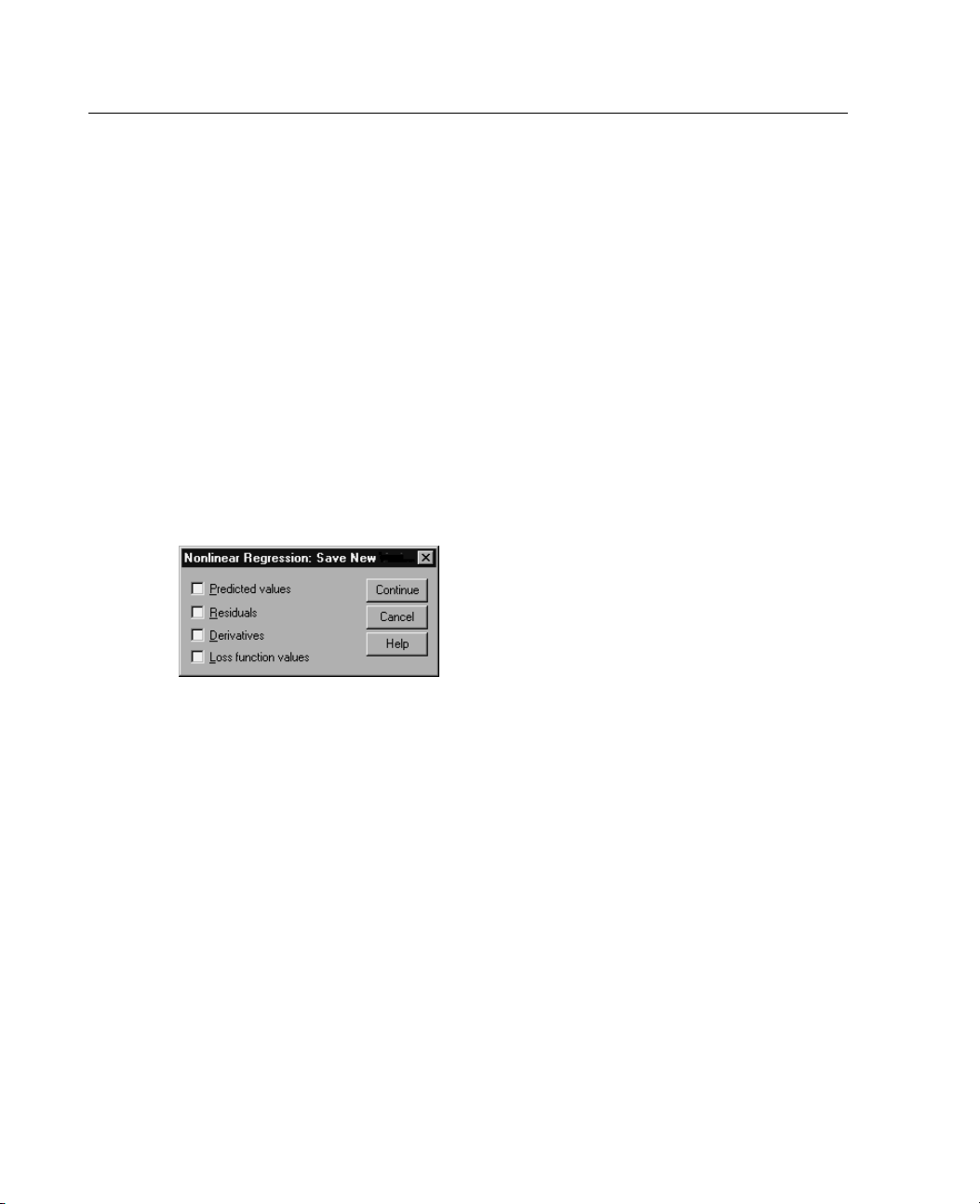
Figure 5-5

Nonlinear Regression Save New Variables dialog box

You can save a number of new variables to your active data file. Available options are
Predicte
can be used in subsequent analyses to test the fit of the model or to identify problem
cases.

 Predicted Values. Saves predicted values with thevariablenamepred_.
 Residuals. Saves residuals with the variable name resid.
 Derivatives. One derivative is saved for each model parameter. Derivative names

 Loss Functio n Values. This option is available if you specify your own loss

Regression Save New Variables

d values, Residuals, Derivatives, and Loss function values. These variables

are created by prefixing 'd.' to the first six characters of parameter names.

functio

n. The variable name loss_ is assigned to the values of the loss function.

39

Nonlinear Re

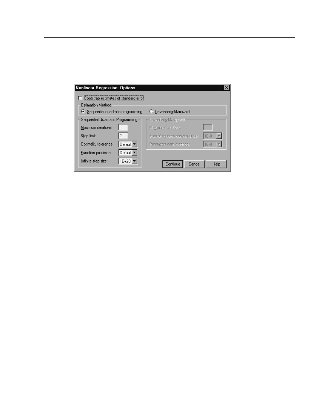
Figure 5-6

Nonlinear Regression Options dialog box

Options allow you to control various aspects of your nonlinear regression analysis:

ap Estimates.

Bootstr

repeated samples from the original data set. This is done by sampling (with
replacement) to get many samples of the same size as the original data set. The

ear equation is estimated for each of these samples. The standard error of each

nonlin
parameter estimate is then calculated as the standard deviation of the bootstrapped
estimates. Parameter values from the original data are used as starting values for each

rap sample. This requires the sequential quadratic programming algorithm.

bootst

gression Options

A method of estimating the standard error of a statistic using

Nonlinear Regr

ession

Estimation Method. Allows you to select an estimation method, if possible. (Certain

choices in this or other dialog boxes require the sequential quadratic programming

ithm.) Available alternatives include Sequential quadratic programming and

algor
Levenberg-Marquardt.

 Sequential Quadratic Programming. This method is available for constrained and

strained models. Sequential quadratic programming is used automatically

uncon
if you specify a constrained model, a user-defined loss function, or bootstrapping.
You can enter new values for Maximum iterations and Step limit, and you can

40

Chapter 5

change the selection in the drop-down lists for Optimality tolerance, Function
precision,

 Levenberg-

and Infinite step size.

Marquardt.

This is the default algorithm for unconstrained models.
The Levenberg-Marquardt method is not available if you specify a constrained
model, a user-defined loss function, or bootstrapping. Y ou can enter new values
for Maximum

iterations, and you can change theselectioninthedrop-downlists

for Sum-of-squares convergence and Parameter convergence.

Interpreting Nonlinear Regression Results

Nonlinear regression problems often present computational difficulties:

 The choice of initial values for the parameters influences convergence. Try to

choose ini
final solution.

 Sometimes one algorithm performs better than the other on a particular problem.

In the Options dialog box, select the other algorithm if it is available. (If you
specify a
Levenberg-Marquardt algorithm.)

 When iteration stops only because the maximum number of iterations has

occurred, the “final” model is probably not a good solution. Select

values fr

or, better yet, choose different initial values.

 Models that require exponentiation of or by large data values can cause overflows

or underflows (numbers t oo large or too small for the computer to represent).
Sometim
constraints on the parameters.

tial values that are reasonable and, if possible, close to the expected

loss function or certain types of constraints, you cannot use the

om previous analysis

in the Parameters dialog box to continue the iteration

es you can avoid these by suitable choice of initial values or by imposing

Use starting

NLR Command Additional Features

The SPSS command language also allows you to:

 Name a file from which to read initial values for parameter estimates.
 Specify more than one model statement and loss function. This makes it easier to

yasegmentedmodel.

specif

 Supply

your own derivatives rather than use those calculated by the program.

41

Nonlinear Regr



Specify the number of bootstrap samples to generate.

 Specify additional iteration criteria, including setting a critical value for derivative

checking and

defining a convergence criterion for the correlation between the

ession

residuals and the derivatives.

Additional

criteria for the

CNLR (constrained nonlinear regression) command allow

you to:

 Specify the maximum number of minor iterations allowed within each major

iteration.

 Set a criti
 Set a step l
 Specify a c

cal value for derivative checking.

imit.
rash tolerance to determine if initial values are within their specified

bounds.

Chapter

6

Weight Estim

Standard linear regression models assume that variance is constant within the
population
are high on some attribute show more variability than cases that are low on that
attribute—linear regression using ordinary least squares (OLS) no longer provides
optimal mo
another variable, the Weight Estimation procedure can compute the coefficients of
a linear regression model using weighted least squares (WLS), such that the more
precise o
determining the regression coefficients. The Weight Estimation procedure tests a
range of weight transformations and indicates which will give the best fit to the data.

Example.

prices? Because stocks with higher share values often show more variability than
those with low share values, ordinary least squares will not produce optimal estimates.
Weight e
of price changes in calculating the linear model.

under study. When this is not the case—for example, when cases that

del estimates. If the differences in variability can be predicted from

bservations (that is, those with less variability) are given greater weight in

What are the effects of inflation and unemployment on changes in stock

stimation allows you to account for the effect of share price on the variability

ation

Statistics. Log-likelihood values for each power of the weight source variable

, multiple R, R-squared, adjusted R-squared, ANOVA table for WLS model,

tested
unstandardized and standardized parameter estimates, and log-likelihood for the
WLS model.

Weight Estimation Data Considerations

Data. The dependent and independent variables should be quantitative. Categorical

variables, such as religion, major, or region of residence, need to be recoded to binary
(dumm
quantitative and should be related to the variability in the dependent variable.

y) variables or other types of contrast variables. The weight variable should be

43

44

Chapter 6

Assumptions. For each value of the independent variable, the distribution of the

dependent variable must be normal. The relationship between the dependent variable
andeachind

ependent variable should be linear, a nd all observations should be
independent. The variance of the dependent variable can vary across levels of the
independent variable(s), but the differences must be predictable based on the weight
variable.

Related procedures. The Explore procedure can be used to screen your data. Explore

provides tests for normality and homogeneity of variance, as well as graphical
displays.

If your dependent variable seems to have equal variance across levels
of independent variables, you can use the Linear Regression procedure. If your
data appear to violate an assumption (such as normality), try transforming them.
If your da

ta are not related linearly and a transformation does not help, use an
alternate model in the Curve Estimation procedure. If your dependent variable is
dichotomous—for example, whether a particular sale is completed or whether an item
is defec

tive—use the Logistic Regression procedure. If your dependent variable is
censored—for example, survival time after surgery—use Life Tables, Kaplan-Meier,
or Cox Regression, available in the SPSS Advanced Models option. If your data
are not i

ndependent—for example, if you observe the same person under several
conditions—use the Repeated Measures procedure, available in the SPSS Advanced
Models option.

Obtaining a Weight Estimation Analysis

E From the menus choose:

Analyze

Regression

Weight Estimation...

45

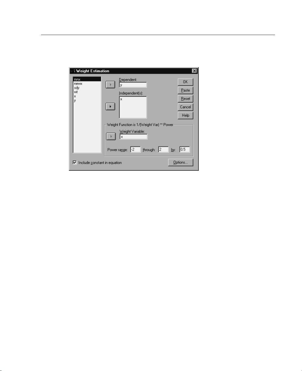
Figure 6-1

Weight Estimation dialog box

E Select one dependent variable.
E Select one or more independent variables.

Weight Estimat

ion

E Select the variable that is the source of heteroscedasticity as the weight variable.

 Weight Variable. The data are weighted by the reciprocal of this variable raised to

a power. The regression equation is calculated for each of a specified range of
power values and indicates the power that maximizes the log-likelihood function.

 Power Range. This is used in conjunction with the weight variable to compute

weights. Several regression equations will be fit, one for each value in the power
range. The values entered in the Power range test box and the through text box
must be between -6.5 and 7.5, inclusive. The power values range from the low to
high value, in increments determined by the value specified. The total number of
values in the power range is limited to 150.

46

Chapter 6

Weight Estim

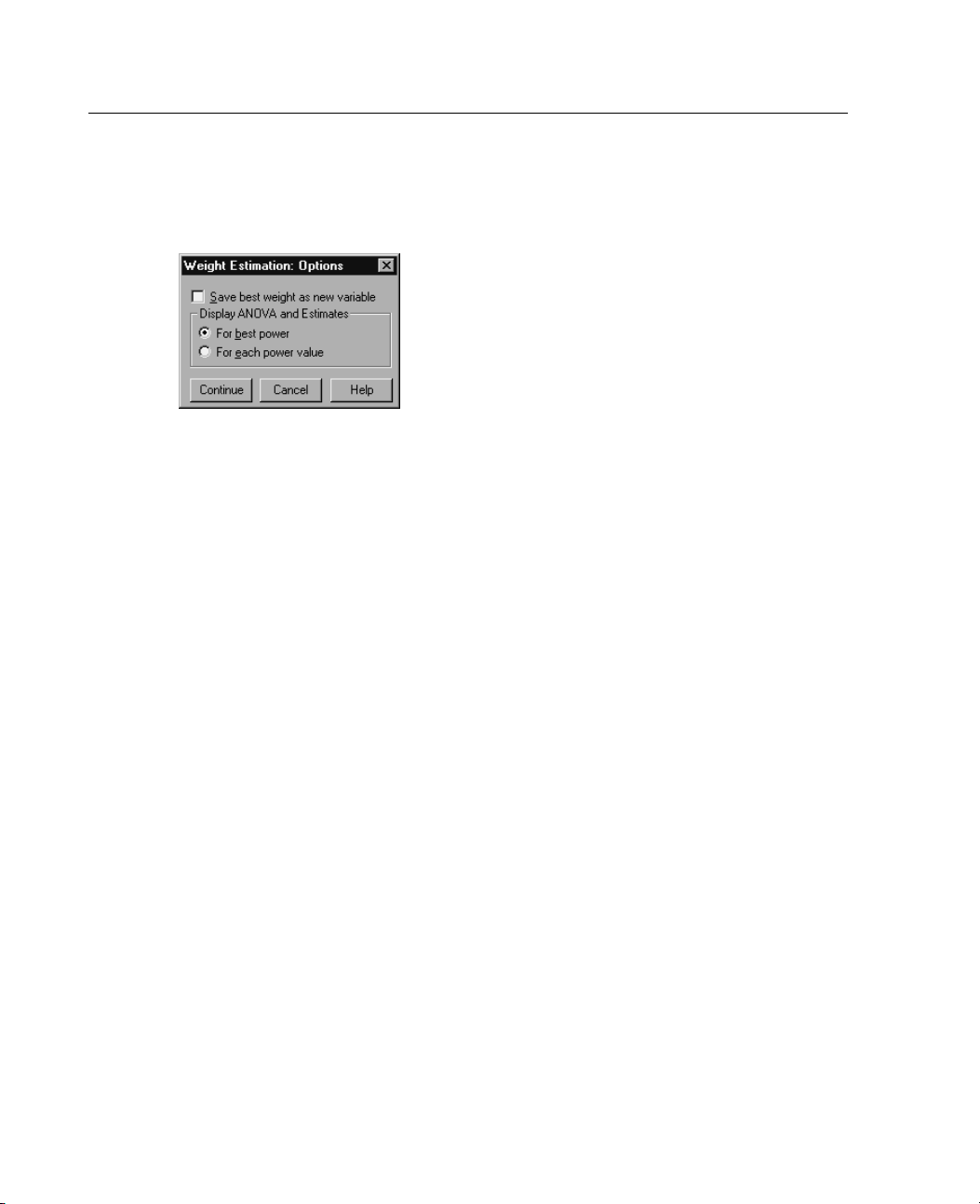
Figure 6-2

Weight Estimation Options dialog box

You can specify options for your weight estimation analysis:

Save best weight as new variable. Addstheweightvariabletotheactivefile.This

variable is called WGT_n,wheren is a number chosen to give the variable a unique
name.

Display ANOVA a nd Estimates. Allows you to control how statistics are displayed in

the output. Available alternatives are For best power and For each power value.

ation Options

WLS Command Additional Features

The SPSS command language also allows you to:

 Provideasinglevalueforthepower.
 Specify a list of power values, or mix a range of values with a list of values for

the power.

Chapter

7

Two-Stage Le
Regression

Standard l
uncorrelated with the independent variable(s). When this is not the case (for example,
when relationships between variables are bidirectional), linear regression using
ordinary l
least-squares regression uses instrumental variables that are uncorrelated with the
error terms to compute estimated values of the problematic predictor(s) (the first
stage), a
of the dependent variable (the second stage). Since the computed values are based
on variables that are uncorrelated with the errors, the results of the two-stage model
are opti

Example. Is the demand for a commodity related to its price and consumers' incomes?

The d ifficulty in this model is that price and demand have a reciprocal effect on each
other. T
two-stage least-squares regression model might use consumers' incomes and lagged
price to calculate a proxy for price that is uncorrelated with the measurement errors in
demand
whichisthenestimated.

inear regression models assume that errors in the dependent variable are

east squares (OLS) no longer provides optimal model estimates. Two-stage

nd then uses those computed values to estimate a linear regression model

mal.

hat is, price can influence demand and demand can also influence price. A

. This proxy is substituted for price itself in the originally specified model,

ast-Squares

Statistics. For each model: standardized and unstandardized regression coefficients,

2

le R, R

multip
predicted values, and residuals. Also, 95% confidence intervals for each regression
coefficient, and correlation and covariance matrices of parameter estimates.

,adjustedR2, standard error of the estimate, analysis-of-variance table,

47

48

Chapter 7

Two-Stage Le

Data. The de

variables, such as religion, major, or region of residence, need to be recoded to binary
(dummy) variables or other types of contrast variables. Endogenous explanatory
variables s

Assumptions. For each value of the independent variable, the distribution of the

dependent variable must be normal. The variance of the distribution of the dependent
variable s
between the dependent variable and each independent variable should be linear.

Related procedures. If you believe that none of your predictor variables is correlated

with the er
procedure. If your data appear to violate one of the assumptions (such as normality
or constant variance), try transforming them. If your data a re not related linearly
and a tran
procedure. If your dependent variable is dichotomous, such as whether a particular
sale is completed or not, use the Logistic Regression procedure. If your data are
not inde
conditions—use the Repeated Measures procedure, available in the SPSS Advanced
Models option.

ast-Squares Regression Data Considerations

pendent and independent variables should be quantitative. Categorical

hould be quantitative (not categorical).

hould be constant for all values of the independent variable. The relationship

rors in your dependent variable, you can use the Linear Regression

sformation does not help, use an alternate model in the Curve Estimation

pendent—for example, if you observe the same person under several

Obtaining a Two-Stage Least-Squares Regression Analysis

E From the menus choose:

Analyze

Regression

2-Stage Least Squ ares...

49

Two-Stage Leas

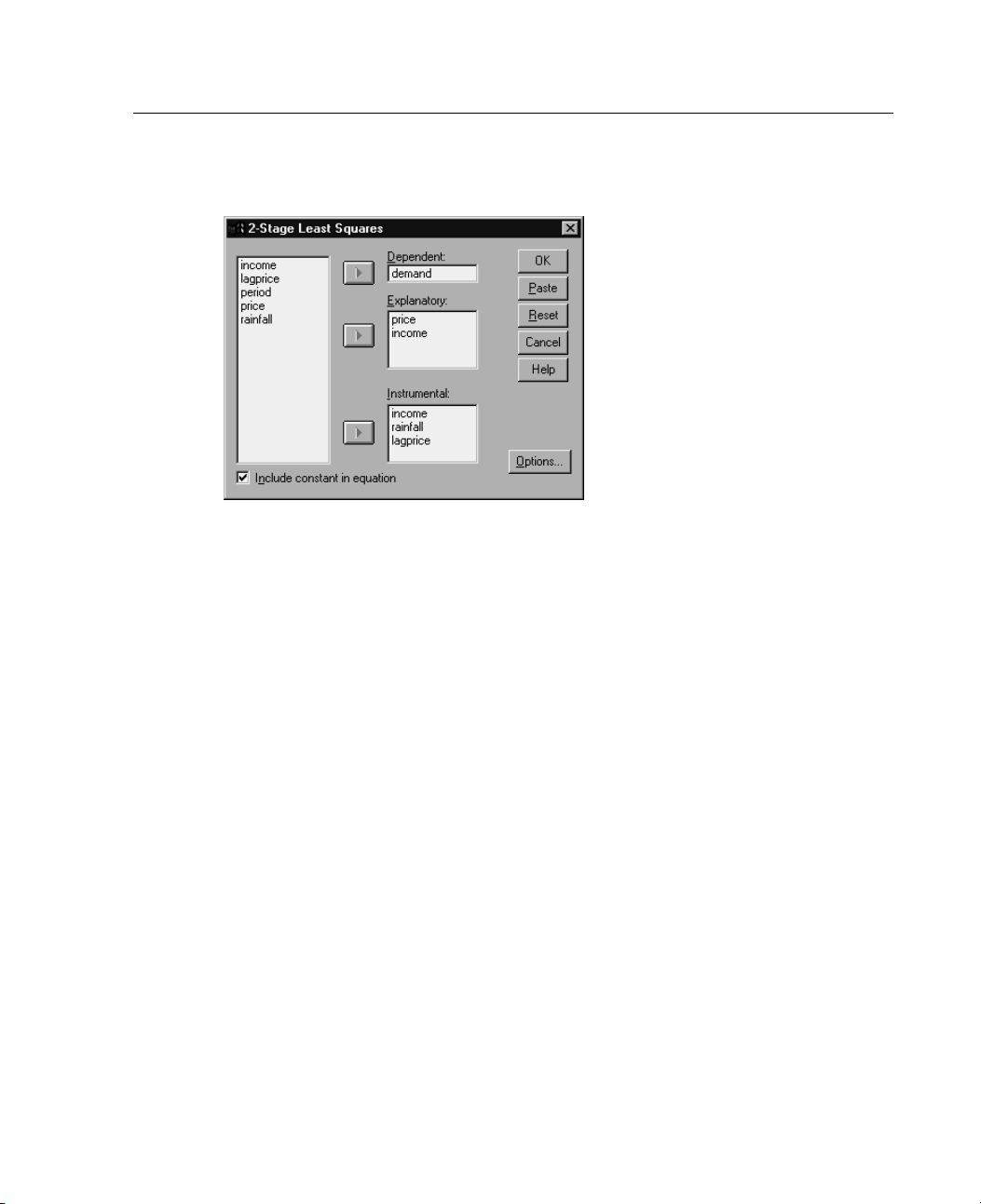
Figure 7-1

2-Stage Least Squares dialog box

E Select one dependent variable.
E Select one or more explanatory (predictor) variables.
E Select one or more instrumental variables.

 Instrumental. These are the variables used to compute the predicted values for the

t-Squares Regression

endogenous variables in the first stage of two-stage least squares analysis. The
same var

iables may appear in both the Explanatory and Instrumental list boxes.
The number of instrumental variables must be at least as many as the number of
explanatory variables. If all explanatory and instrumental variables listed are the

he results are the same as results from the Linear Regression procedure.

same, t

Explanatory variables not specified as instrumental are considered endogenous.
Normally, all of the exogenous variables in the Explanatory list are also specified as

mental variables.

instru

50

Chapter 7

Two-Stage Le

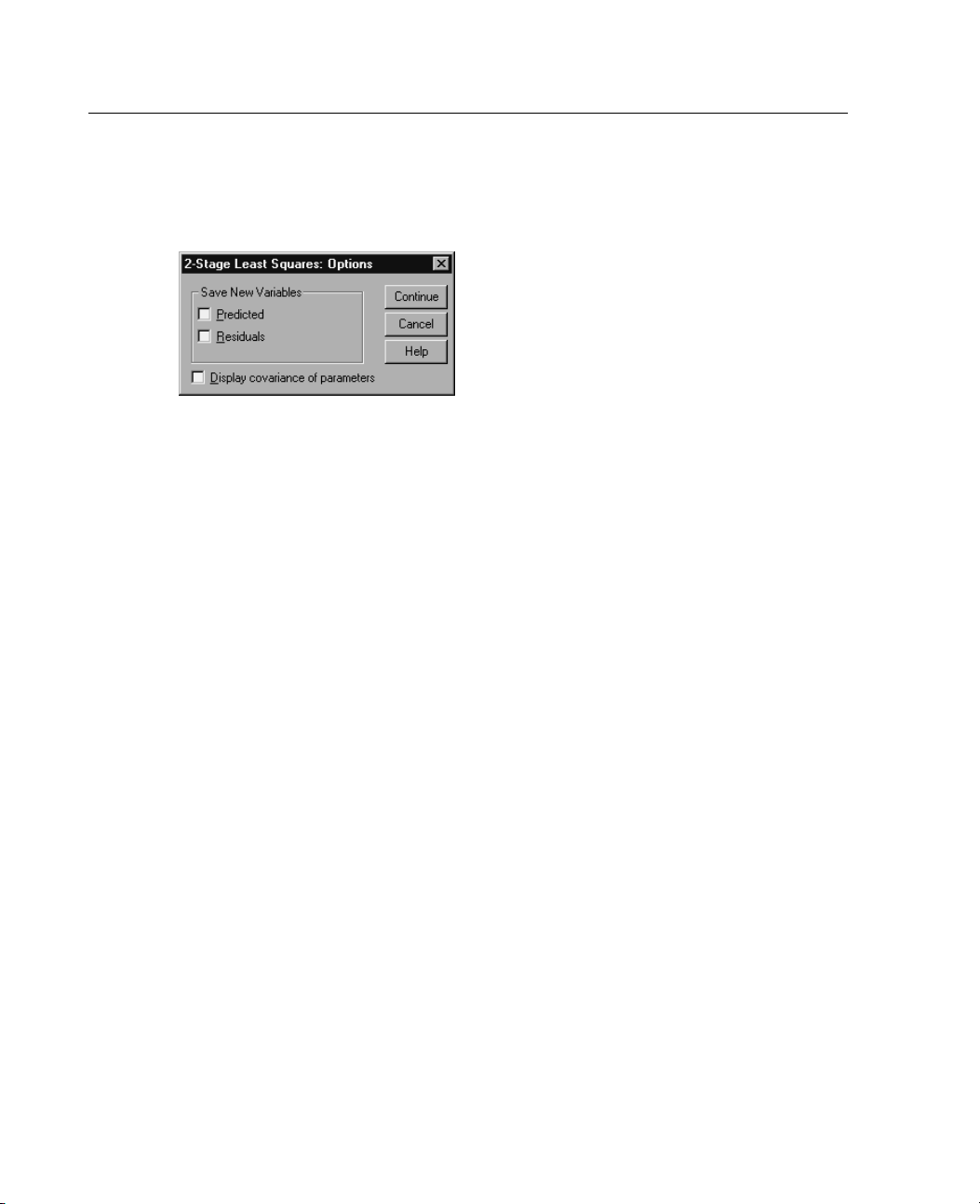
Figure 7-2

2-Stage Least Squares Options dialog box

You can select the following options for your analysis:

Save New Variables. Allows you to add new variables to your active file. Available

options are Predicted and Residuals.

Display covariance of parame ters. Allows you to print the covariance matrix of the

parameter estimates.

ast-Squares Regression Options

2SLS Command Additional Features

The SPSS command language also allows you to estimate multiple equations
simultaneously.

Appendix

A

Categorical
Schemes

S procedures, you can request automatic replacement of a categorical

ded, usually on the

n from the grand mean.

(1/k 1/k

( 1–1/k –1/k

( –1/k 1–1/k

..
..

( –1/k –1/k

Deviatio

In many SPS
independent variable with a set of contrast variables, which will then be entered or
removed from an equation as a block. You can specify how the set of contrast variables
is to be co
illustrates how different contrast types requested on CONTRAST actually work.

n

Deviatio

mean

df(1)
df(2)

df(k–1)

Variable Coding

CONTRAST subcommand. This appendix explains and

In matrix terms, these contrasts have the form:

...
...
...

...

1/k 1/k )
–1/k –1/k )
–1/k –1/k )

1–1/k –1/k )

where k is the number of categories for the independent variable and the last category
is omitted by default. For example, the deviation contrasts for an independent variable
with three categories are as follows:

( 1 /3 1/3 1/3 )
( 2/3 –1/3 –1/3 )

( –1 /3 2/3 –1/3 )

51

52

Appendix A

Simple

To omit a category other than the last, specify the number of the omitted category in
parentheses after the DEVIATION keyword. For example, the following subcommand
obtains the

/CONTRAST(FACTOR)=DEVIATION(2)

deviations for the first and third categories and omits the second:

Suppose that factor has three categories. The resulting contrast matrix will be

( 1 /3 1/3 1/3 )
( 2/3 –1/3 –1/3 )

( –1 /3 –1/3 2/3 )

Simple contrasts. Compares each level of a factor to the last. The general matrix

form is

mean

df(1) ( 1 0
df(2) ( 0 1

df(k–1) ( 0 0

(1/k 1/k

..
..

...
...
...

...

1/k 1/k )

0–1)
0–1)

1–1)

where k is the number of categories for the independent variable. For example, the
simple contrasts for an independent variable with four categories are as follows:

( 1/4 1/4 1/4 1/4 )

(100–1)
(010–1)
(001–1)

To use another category instead of the last as a reference category, specify in
parentheses after the SIMPLE keyword the sequence number of the reference category,
which is not necessarily the value associated with that category. For example, the

53

Helmert

Categorical Va

riable Coding Schemes

following CONTRAST subcommand obtains a contrast matrix that omits the second
category:

/CONTRAST(FACTOR) = SIMPLE(2)

Suppose that factor has four categories. The resulting contrast matrix will be

( 1/4 1/4 1/4 1/4 )

(1 –1 0 0)
(0 –1 1 0)
(0 –1 0 1)

Helmert contrasts. Compares categories of an independent variable with the mean of

the subsequent categories. The general matrix form is

mean

df(1) ( 1
df(2) ( 0 1

..
..

df(k–2) ( 0 0 1 –1/2 –1/2
df(k–1) ( 0 0

(1/k 1/k

–1/(k–1)

...
...
...

...

1/k 1/k )
–1/(k–1) –1/(k–1) )
–1/(k–2) –1/(k–2) )

1–1)

where k is the number of categories of the independent variable. For example, an
independent variable with four categories has a Helmert contrast matrix of the
following form:

( 1/4 1/4 1/4 1/4 )

( 1 –1/3 –1/3 –1/3 )
( 0 1 –1/2 –1/2 )
(001–1)

54

Appendix A

Difference

Difference

variable with the mean of the previous categories of the variable. The general matrix
form is

df(k–1)

where k is the number of categories for the independent variable. For example, the
difference contrasts for an independent variable with four categories are as follows:

( –1/2 –1/2 1 0 )
( –1/3 –1/3 –1/3 1 )

Polynomial

Orthogonal polynomial contrasts. The first degree of freedom contains the linear effect

across all categories; the second degree of freedom, the quadratic effect; the third
degree of freedom, the cubic; and so on, for the higher-order effects.

You can specify the spacing between levels of the treatment measured by the given
categorical variable. Equal spacing, which is the default if you omit the metric, can be
specified as consecutive integers from 1 to k,wherek is the number of categories. If
the variable drug has three categories, the subcommand

or rever se Helmert contrasts.

mean

df(1) ( –1 1 0
df(2) ( –1/2 –1/2 1

..
..

( 1/4 1/4 1/4 1/4 )

(–1100)

(1/k 1/k 1/k

( –1/(k–1) –1/(k–1) –1/(k–1)

Compares categories of an independent

...

1/k )

...
...

...

0)

0)

1)

/CONTRAST(DRUG)=POLYNOMIAL

is the same as

/CONTRAST(DRUG)=POLYNOMIAL(1,2,3)

55

Categorical Va

riable Coding Schemes

Equal spacing is not always necessary, however. For example, suppose that
drug represents different dosages of a drug given to three groups. If the dosage
administer

ed to the second group is twice that given to the first group and the dosage
administered to the third group is three times that given to the first group, the
treatment categories are equally spaced, and an appropriate metric for this situation
consists o

/CONTRAST(DRUG)=POLYNOMIAL(1,2,3)

f consecutive integers:

If, however, the dosage administered to the second group is four times that given to
the first g

roup, and the dosage administered to the third group is seven times that

given to the first group, an appropriate metric is

/CONTRAST

In either c

(DRUG)=POLYNOMIAL(1,4,7)

ase, the result of the contrast specification is that the first degree of freedom
for drug contains the linear effect of the dosage levels and the second degree of
freedom contains the quadratic effect.

Polynomi

al contrasts are especially useful in tests of trends and for investigating
the nature of response surfaces. You can also use polynomial contrasts to perform
nonlinear curve fitting, such as curvilinear regression.

Repeated

Compares adjacent levels of an independent variable. The general matrix form is

where k is the number of categories for the independent variable. For example, the
repeated contrasts for an independent variable with four categories are as follows:

mean

df(1) ( 1 –1 0
df(2) ( 0 1 –1

df(k–1) ( 0 0 0

(1/k 1/k 1/k

..
..

...
...
...

...

1/k 1/k )

00)

00)

1–1)

56

Appendix A

Special

( 1/4 1/4 1/4 1/4 )

(1 –1 0 0)
(0 1 –1 0)
(0 0 1 –1)

These contrasts are useful in profile analysis and wherever difference scores are
needed.

A user-defined contrast. Allows entry of special contrasts in the form of square

matrices with as many rows and columns as there are categories of the given
independent variable. For MANOVA and LOGLINEAR, the first row entered is always
the mean, or constant, effect and represents the set of weights indicating how to
average other independent variables, if any, over the given variable. Generally, this
contrastisavectorofones.

The remaining rows of the matrix contain the special contrasts indicating the
desired comparisons between categories of the variable. Usually, orthogonal contrasts
are the most useful. Orthogonal contrasts are statistically independent and are
nonredundant. Contrasts are orthogonal if:

 For each row, contrast coefficients sum to 0.
 The products of corresponding coefficients for all pairs of disjoint rows also

sum to 0.

For example, suppose that treatment has four levels and that you want to compare the
various levels of treatment with each other. An appropriate special contrast is

( 1 1 1 1 ) weights for mean calculation

st

( 3 –1 –1 –1 ) compare 1
(0 2 –1 –1) compare2ndwith 3rdand 4
( 0 0 1 –1 ) compare 3rdwith 4

with 2ndthrough 4

th

th

th

which you specify by means of the following CONTRAST subcommand for MANOVA,

LOGISTICREGRESSION,andCOXREG:

57

Categorical Va

/CONTRAST(TREATMNT)=SPECIAL( 1111

3-1-1-1
0 2 -1 -1
001-1)

riable Coding Schemes

For LOGLINEAR, you need to specify:

/CONTRAST(T

Each row excep

REATMNT)=BASIS SPECIAL( 1111

3-1-1-1
0 2 -1 -1
001-1)

t the means row sums to 0. Products of each pair of disjoint rows

sumto0aswell:

Rows 2 and 3: (3)(0) + (–1)(2) + (–1)(–1) + (–1)(–1) = 0
Rows 2 and 4: (3)(0) + (–1)(0) + (–1)(1) + (–1)(–1) = 0
Rows 3 and 4: (0)(0) + (2)(0) + (–1)(1) + (–1)(–1) = 0

The special contrasts need not be orthogonal. However, they must not be linear
combinations of each other. If they are, the procedure reports the linear dependency

nd ceases processing. Helmert, d ifference, and polynomial contrasts are all

a
orthogonal contrasts.

ndicator

I

ndicator variable coding.

I

LOGLINEAR or MANOVA. The number of new variables coded is k–1. Cases in the

Also known as dummy coding, this is not available in

reference category are coded 0 for all k–1 variables. A case in the ithcategory is

th

coded 0 for all indicator variables except the i

, which is coded 1.

Index

asymptotic regression, 35

in Nonlinea

backward elimination, 6

in Logistic Regression, 6

binary logistic regression, 1
categorical covariates, 7

cell probabilities tables, 18

in Multinomi

cells with zero observations, 19

in Multinomial Logistic Regression, 19

classification, 13

in Multinomial Logistic Regression, 13

classification tables, 18

in Multinomia

confidence intervals, 18

in Multinomial Logistic Regression, 18

constant term, 10

in Linear Regression, 10

constrained regression

in Nonlinear Re

contrasts, 7

in Logistic Regression, 7

convergence criterion, 19

in Multinomial Logistic Regression, 19

Cook's D, 9

in Logistic Reg

correlation matrix, 18

in Multinomial Logistic Regression, 18

covariance matrix, 18

in Multinomial Logistic Regression, 18

covariates

in Logistic Regr

Cox and Snell R-square, 18

in Multinomial Logistic Regression, 18

custom models, 15

in Multinomial Logistic Regression, 15

delta, 19

as correction fo

density model, 35

in Non linear Regression, 35

deviance function, 21

for estimating dispersion scaling value, 21

r Regression, 35

al Logistic Regression, 18

l Logistic Regression, 18

gression, 37

ression, 9

ession, 7

r cells with zero observations, 19

DfBeta, 9

in Logistic

dispersion scaling value, 21

in Multinomial Logistic Regression, 21

fiducial confidence intervals, 28

in Probit Analysis, 28

forward selection, 6

in Logistic R

full factorial models, 15

in Multinomial Logistic Regression, 15

Gauss model, 35

in Nonlinear Regression, 35

Gompertz model, 35

in Nonlinear R

goodness of fit, 18

in Multinomial Logistic Regression, 18

Hosmer-Lemeshow goodness-of-fit statistic, 10

in Logistic Regression, 10

intercept, 15

include or exc

iteration history, 19

in Multinomial Logistic Regression, 19

iterations, 10, 19, 28

in Logistic Regression, 10
in Multinomial Logistic Regression, 19
in Probit Analy

Johnson-Schumacher m o del, 35

in Nonlinear Regression, 35

leverage values, 9

in Logistic Regression, 9

likelihood ratio, 18, 21

for estimating
goodness of fit, 18

Linear Regression, 43, 47

Two-Stage Least-Squares Regression, 47
weight estimation, 43

logistic regression, 1

binary, 1

Logistic Regression, 3 , 6

assumptions, 4
categorical covariates, 7

Regression, 9

egression, 6

egression, 35

lude, 15

sis, 28

dispersion scaling value, 21

59

60

Index

classification cutoff, 10
coefficients, 3
command addi

tional features, 11
constant term, 10
contrasts, 7
data considerations, 4
define selection rule, 6
dependent variable, 4
display optio

ns, 10
example, 3
Hosmer-Lemeshow goodness-of-fit statistic, 10
influence measures, 9
iterations, 10
predicted values, 9
probability fo

r stepwise, 10
related procedures, 4
residuals, 9
saving new variables, 9
set rule, 6
statistics, 3
statistics and

plots, 10
string covariates, 7
variable selection methods, 6

log-likelihood, 18, 43

in Multinomial Logistic Regression, 18
in We ight Estimation, 43

log-modified mo

del, 35
in Non linear Regression, 35

main-effects models, 15

in Multinomial Logistic Regression, 15

McFadden R-square, 18

in Multinomial Logistic Regression, 18

Metcherlich law

of diminishing returns, 35

in Non linear Regression, 35

Michaelis Menten model, 35

in Non linear Regression, 35

Morgan-Mercer-Florin model, 35

in Non linear Regression, 35

Multinomial Logi

stic Regression, 13, 13, 15, 18,

19, 22, 23
assumptions, 13
command additionalfeatures,23
criteria, 19
exporting model information, 22
models, 15

reference category, 17
save, 22
statistics,

18

Nagelkerke R-square, 18

in Multinomial Logistic Regression, 18

nonlinear models, 35

in Nonlinear Regression, 35

Nonlinear Regression, 31, 35

assumptions,

32
bootstrap estimates, 39
command additionalfeatures,40
common nonlinear models, 35
conditional logic, 33
data considerations, 32
derivatives, 3

8
estimation methods, 39
example, 31
interpretation of results, 40
Levenberg-Marquardt algorithm, 39
loss function, 36
parameter c ons

traints, 37
parameters, 34
predicted values, 38
related procedures, 32
residuals, 38
save new variables, 38
segmented model

,33
sequential quadratic programming, 39
starting values, 32, 34
statistics, 31

parallelism test, 28

in Probit Analysis, 28

parameter const

raints

in Nonlinear Regression, 37

parameter estimates, 18

in Multinomial Logistic Regression, 18

Peal-Reed model, 35

in Nonlinear Regression, 35

Pearson chi-squa

re, 18, 21
for estimating dispersion scaling value, 21
goodness of fit, 18

Probit Analysis, 25

assumptions, 25
command additionalfeatures,29
criteria, 28

61

Index

data considerations, 25
define range, 28
example, 25
fiducial confidence intervals, 28
iterations, 28
natural response r ate, 28
parallelism test, 28
related procedures, 25
relative medi

an potency, 28

statistics, 25, 28

ratio of cubics model, 35

in Non linear Regression, 35

ratio of quadratics m odel, 35

in Non linear Regression, 35

reference cate

gory

in Multinomial Logistic Regression, 17

relative median potency, 28

in Probit Analysis, 28

Richards model, 35

in Non linear Regression, 35

separation, 19

in Multinomial Logistic Regression, 19

singularity, 19

in Multinomial Logistic Regression, 19

step-halving, 19

in Multinomial Logistic Regression, 19

stepwise select

ion, 6 , 15
in Logistic Regression, 6
in Multinomial Logistic Regression, 15

string covariates, 7

in Logistic Regression, 7

Two-Stage Least-Squares Regression, 47, 48, 50, 50

assumptions, 48
command addi

tional features, 50
covariance of parameters, 50
data considerations, 48
example, 47
instrumental variables, 47
related procedures, 48
saving new var

iables, 50

statistics, 47

Verhulst model, 35

in Nonlinear Regression, 35

Von Bertalanffy model, 35

in Nonlinear Regression, 35

Weibull m odel

,35

in Nonlinear Regression, 35

Weight Estimation, 43

assumptions, 43
command additionalfeatures,46
data considerations, 43
display ANOVA a

nd estimates, 46
example, 43
iteration history, 46
log-likelihood, 43
related procedures, 43
save best weights as new variable, 46
statistics, 43

yield density model, 35

in Nonlinear Regression, 35