Spss CONJOINT 8.0 User Manual

SPSS Conjoint™ 8.0

For more information about SPSS® software products, please visit our WWW site at
http://www.spss.com or contact

Marketing Depart ment
SPSS Inc.
233 South Wacker Drive, 11th Floor
Chicago, IL 60606-6412
Tel: [phone]
Fax: [phone]

SPSS is a registered trademark and the other product names are the trademarks of SPSS Inc.
for its proprietary computer software. No material describing such software may be produced
or distributed without the written permission of the owners of the trademark and license rights
in the software and the copyrights in the published materials.

The SOFTWARE and documentation are provided with RESTRICTED RIGHTS. Use,
duplication, or disclosure by the Government is subject to restrictions as set forth in
subdivision (c)(1)(ii) of The Rights in Technical Data and Computer Software clause at

52.227-7013. Contractor/manufacturer is SPSS Inc., 233 South Wacker Drive, 11th Floor,
Chicago, IL 60606.

General notic e : Other product names mentione d herein are used for identifi c ation purposes
only and may be trademarks of their respective companies.

Windows is a registered trademark of Microsoft Corporation.
SPSS Conjoint

™

8.0

Copyright © 1997 by SPSS Inc.
All rights reserved.
Printed in the United States of America.

No part of this publication may be reproduced, stored in a retrieval system, or transmitted, in
any form or by any means, electronic, mechanical, photocopying, recording, or otherwise,
without the prior written permission of the publisher.

7 8 9 0 05 04 03 02
ISBN 1-56827-212-X

Preface

SPSS® 8.0 is a powerful software package for data management and analysis. The
Conjoint option is an add-on enhancement that provides a comprehensive set of
procedures for conjoint analysis. The procedures in Conjoint must be used with the
SPSS Base system and are comp letely integrated into that system.

The Conjoint option includes:

 Procedures for developing and producing profiles for use in conjoint studies.
 Four different models for conjoint analysis.
 Graphic summary of conjoint results.

Compatibility

The SPSS system is designed to operate on many computer systems. See th e materials
that came with your system for specific informati on o n mini mum an d recommen ded
requirements.

Customer Service

If you have any questions concerning your shipment or account, contact your local
office, listed on page v. Please have y our serial nu mber ready for i dentification when
calling.

iii

Training Seminars

SPSS Inc. provides both public and onsite training seminars. All seminars feature
hands-on workshops. Seminars will be offered in major cities on a regular basis. For
more information on these seminars, call your local office, listed on page v.

Technical Support

The services of SPSS Technical Support are available to registered customers.
Customers may contact T echni cal Support for assistance in using SP SS products or for
installation help for one of the supported hardware environments. To reach Technical
Support, see the SPSS home page on the W orld Wide W e b at http://www.spss.com, or
call your local office, listed on page v. Be prepared to identify yourself, your
organization, and the serial number of your system.

Tell Us Your Thoughts

Your comments are important. Please send us a letter and let us know about your
experiences with SPSS produc ts. We especially like to hear abou t new and i ntere sting
applications using the SPSS syst em. W rite to SPS S Inc. Marketing Department, Attn.:
Director of Product Planning, 444 N. Michigan Avenue, Chicago, IL 60611.

About This Manual

This manual is divided into two parts. The first part provides a guide to the various
statistical techniques available with the Conjoint option and how to obtain the
appropriate statistical analyses with the dialog box interface. The second part is a
Syntax Reference section that provides complete command syntax for all of the
commands included in the Conjoint option. Most features of the system can be
accessed through the dialog box interface, but some functi onality can be accessed only
through command syntax.

This manual contains two in dexes: a subject index and a syntax index . The subj ect
index covers both secti ons of the manua l. The syntax i ndex ap plies only to t he Synt ax
Reference section.

iv

Contents

1 Introduction to Conjoint Analysis 1

Why Use Conjoint Analysis? . . . . . . . . . . . . . . . . . . . . . . . . . . 2

The Full-Concept Method . . . . . . . . . . . . . . . . . . . . . . . . . . . . 4

An Orthogonal Array . . . . . . . . . . . . . . . . . . . . . . . . . . . . 5

The Experimental Stimuli. . . . . . . . . . . . . . . . . . . . . . . . . . 5

Collecting and Analyzing the Data . . . . . . . . . . . . . . . . . . . . 6

2 Designing the Conjoint Study:

Generating an Orthogonal Design

The Carpet-Cleaner Study. . . . . . . . . . . . . . . . . . . . . . . . . . . . 8

An Orthogonal Array . . . . . . . . . . . . . . . . . . . . . . . . . . . . . . .9

Generating an Orthogonal Design . . . . . . . . . . . . . . . . . . . . . . . 9

Entering Simulation Cases . . . . . . . . . . . . . . . . . . . . . . . . 11

What’s Next? . . . . . . . . . . . . . . . . . . . . . . . . . . . . . . . . . . 12

How to Obtain an Orthogonal Design . . . . . . . . . . . . . . . . . . . . 12

Output File Specification . . . . . . . . . . . . . . . . . . . . . . . . . 14

Define Values . . . . . . . . . . . . . . . . . . . . . . . . . . . . . . . 15

Options . . . . . . . . . . . . . . . . . . . . . . . . . . . . . . . . . . . 16

Additional Features Available with Command Syntax . . . . . . . . 17

7

vii

3 Creating the Experimental Stimuli:

Displaying the Design

Creating the Carpet-Cleaner Profiles . . . . . . . . . . . . . . . . . . . . 19

How to Display an Orthogonal Design . . . . . . . . . . . . . . . . . . . 22

How to Display Orthogonal Design Titles . . . . . . . . . . . . . . . 23

Additional Features Available with Command Syntax . . . . . . . . 24

4 Analyzing Preferences:

Using the Conjoint Procedure

Collecting the Data. . . . . . . . . . . . . . . . . . . . . . . . . . . . . . . 25

Analyzing Carpet-Cleaner Preference. . . . . . . . . . . . . . . . . . . . 26

Relative Importance . . . . . . . . . . . . . . . . . . . . . . . . . . . 29

The Holdouts and Simulations . . . . . . . . . . . . . . . . . . . . . 30

Subfile Summary . . . . . . . . . . . . . . . . . . . . . . . . . . . . . 31

The Utility File . . . . . . . . . . . . . . . . . . . . . . . . . . . . . . . 34

How to Obtain a Conjoint Analysis . . . . . . . . . . . . . . . . . . . . . . 34

Minimum Specifications . . . . . . . . . . . . . . . . . . . . . . . . . 35

Specifying the Files. . . . . . . . . . . . . . . . . . . . . . . . . . . . 35

Specifying How Data Were Recorded . . . . . . . . . . . . . . . . . 35

Optional Specifications . . . . . . . . . . . . . . . . . . . . . . . . . 37

19

25

viii

Syntax Reference 39

Introduction . . . . . . . . . . . . . . . . . . . . . . . . . . . . . . . . . . 41

CONJOINT . . . . . . . . . . . . . . . . . . . . . . . . . . . . . . . . . . . 45

ORTHOPLAN . . . . . . . . . . . . . . . . . . . . . . . . . . . . . . . . . . 56

PLANCARDS . . . . . . . . . . . . . . . . . . . . . . . . . . . . . . . . . . 61

Bibliography 69

Subject Index 71

Syntax Index 75

ix

Introduction to Conjoint Analysis

Market research is frequently concerned with finding out which characteristics of a
product or service are most important to consumers. The ideal product or service, of
course, would have all the best characteristics, but realistically, tradeoffs have to be
made. The product with the most expensive features, for example, cannot have the
lowest price.

Conjoint analysis is a technique for measuring consumer preferences about the
attributes of a product or service. There are tw o general approaches to collect ing data
for conjoint analysis—the two-factor-at-a-time tradeoff method and the multiple
factor full-concept method. With the tradeoff method, respondents are asked to rank
the cells of a series of matrices, each matrix crossin g the levels of one factor wi th the
levels of another.

The two-factor-at-a-time tradeoff method is hardly ever used today. The full­concept method, which will be explained in detail in this chapter, is considered a more
realistic, ecologically valid method because all factors are considered at the same
time. The three conjoint analysis proced ures—Generate Orthogonal Design, Displ ay
Design, and Conjoint—are designed for the full-concept method. For more
explanation of the tradeoff method and comparisons with the full-concept method, see
Aaker and Day (1986).

Chapter

1

1

2

Chapter 1

Why Use Conjoint Analysis?

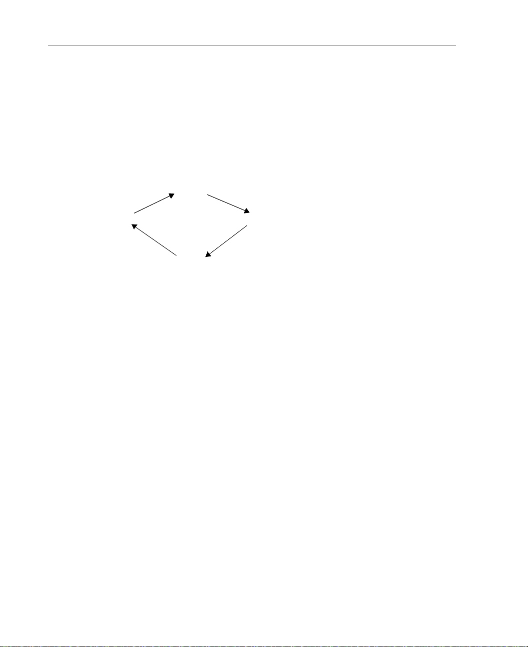
The Deming Cycle, origin ated by W. Edwards Deming and pictured in Figure 1-1, is a
convenient model for thinking about the production of consumer goods.

Figure 1-1
The Deming Cycle

design

research

sales

manufacturing

Design and manufacturing are the responsib ility of la boratories an d engineers. Sales is
the responsibility of the sales department. Market researc h is the responsibility of the
marketing department.

Effective market research is integral to the design, manufacture, and sale of
successful products. It identifies the needs and wants of target markets, ensuring that
products will sell because they meet the needs of buyers.

Conjoint analysis is a mar ket research to ol for devel oping effect ive product design.
Using conjoint analysis, the researcher can answer questions such as: What product
attributes are important or unimportant to the consumer? What levels of product
attributes are the most or least desirable ones in the consumer’s mind? What is the
market share of preference for leading competitors’ products versus our existing or
proposed product? Answers to these quest ions ar e of cruci al i mport ance in the design
and launch of a successful product.

The virtue of conjoint analysis is t hat it asks the responden t t o make cho ices in t he
same fashion as the consumer presumably does—by trading off features, one against
another.

For example, suppose that you want to book an airline flight. You have the choice
of sitting in a cramped seat or a spaciou s seat. If this were t he only considera tion, your
choice would be clear. You would probably prefer a spacious seat. Or suppose you
have a choice of ticket prices: $225 or $800. On price alone, taking nothing else into
consideration, the lower price would be preferable. Finally, suppose you can take

Introduction to Conjoint Analysis

either a direct flight, which takes two hours, or a flight with one layo ver, which ta kes
five hours. Most people would choose the direct flight.

The drawback of the above approach is that choice alternatives are presented on
single attributes alone, one at a time. Conjoint analysis presents choice alternatives
between products defined by sets of attributes. This is illustrated by the following
choice: would you prefer a flight that is cramped, costs $225, and has one layover, or
a flight that is spacious, co sts $800, and is direct? Extending this, we see that if
comfort, price, and duration are the relevant attributes, there are potentially eight
products:

Comfort Price Duration

1 cramped $225 2 hours
2 cramped $225 5 hours
3 cramped $800 2 hours
4 cramped $800 5 hours
5 spacious $225 2 hours
6 spacious $225 5 hours
7 spacious $800 2 hours
8 spacious $800 5 hours

3

Given the above alternatives, pr oduct 4 is pro bably the least pr eferred while product 5
is probably the most preferred. The preferences of respondents for the other product
offerings are implicitly determined by what is important to the respondent.

Using conjoint analysis, you can determine both the relat ive importance of each
attribute as well as which levels of each attribute are most preferred. If the most
preferable product is not feasible for some reason, such as cost, you would know the next
most preferred alternative. If you have other information on the r esponden ts, such as
background demographics, you might be able to ident i fy market segments f or which
distinct products can be packaged. For example, the business traveler and the student
traveler might have different preferences that could be met by distinct produ ct offering s.

SPSS Conjoint uses the full-concept a p proach for conjoint analysis. In the full­concept approach, respondents rank alternative products def ined by particular lev els of
all attributes, as in the example above. The full-concept approach in Conjoint uses
what are termed fractional factorial designs, which present a suitable fraction of all
possible alternatives. Fractional designs are used when presenting all alternatives
would be too time-consuming, cost too much, or fatigue the respondent, thereby
potentially invalidating the responses. The Generate Orthogonal Design procedure
automatically generates main-effects orthogonal fractional factorial plans. The Display

4

Chapter 1

Design procedure enables you to generate physical profiles that can be sorted by the
respondent to arrive at a ranking.

The Conjoint procedure performs conj oint analysis usi ng the ordinary least-squares
estimation method. This method has been fo und t o perf orm as well as other metho ds,
and it has the advantage of being easier to use and interpret.

Output from conjoint analysis includes importance ratings of the attributes, part­worth estimates showing preferences for attribute alternatives, and correlations
relating predicted rankings from the conjoint model with observed rankings.

You can specify holdout cards, which are useful for vali da ti ng t he conj oint model .
You can also specify simulation cards, whic h represent actual or prospective produc ts
for which the Conjoint procedure can be used to estimate market share of preference
using several popular models.

The Full-Concept Method

In the full-concept (also known as full-profile) method, the respondent is asked to rank,
order, or score a set of profiles, or cards, according to preference. On each of these
profiles, all factors of interest are represented and a different combination of factor levels
(features) appears. In this way, a full co ncept (that is, a complete product or service) is
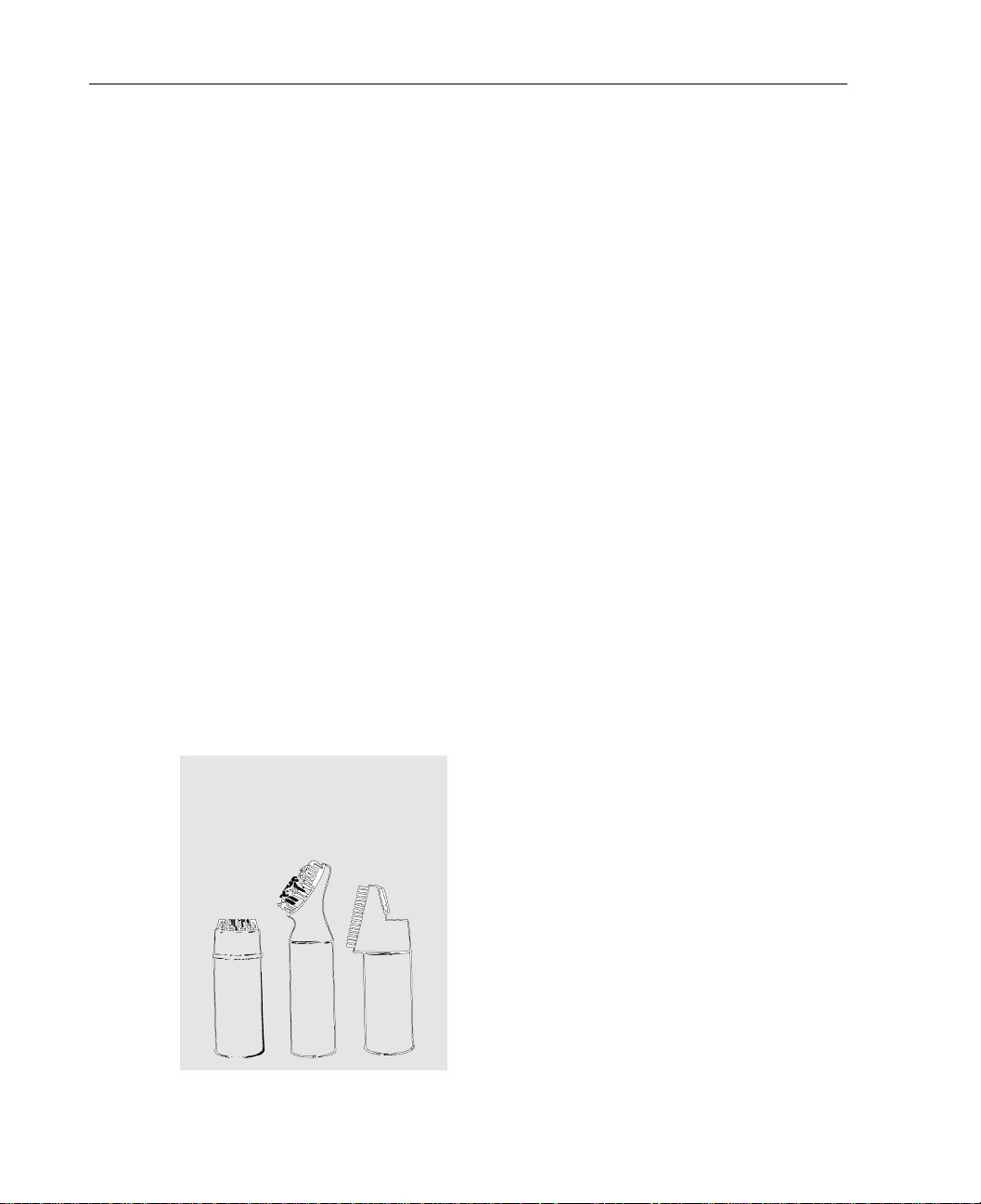
described on each profile. An example of such a profile is shown in Figure 1-2.

Figure 1-2

Full-concept profile (drawings reprinted with permission from Green and Wind, 1973)

A New Carpet Cleaner
Package Design A*

Brand Name GLORY
Price $1.19
Good Housekeeping Seal? YES
Moneyback Guarantee? NO

*Package Designs

AB

C

The respondent’s task is to rank or score each profile from most to least preferred, most
to least likely to purchase, or some other preference scale. From these rankings or
scores, conjoint analysis derives utility scores for each fa ctor level. These utility scores,
analogous to regression coefficients, are called part-worths and can be used to find the
relative importance of each factor. Such information can be very useful when deciding
which combination of factor levels is best for a new product or service and when
predicting various outcomes, such as sales, given certain combinations of factor levels.

An Orthogonal Array

A potential problem with the full-concept method soon becomes obvious if more than
a few factors are involved and each factor has more than a couple of levels. The total
number of profiles resulting from all possibl e combinati ons of the levels becomes too
great for respondents to rank or scor e in a meanin gful way. For this reason, frequen tly
only a subset of all possible profiles is used in the experiment. The subset, called an
orthogonal array, is a type of design in which only main effects are considered and
interactions are assumed to be negligible.

The Generate Orthogonal Design procedure generates an orthogonal main-effects
plan. From the factors and levels specified, Generate Orthogonal Design can either
create a new working data file containing the orthogonal plan or it can replace the
current working data file.

5

Introduction to Conjoint Analysis

The Experimental Stimuli

As discussed in “Collecting and Analyzing the Data” below, data collection in a full­concept design requires that the stimuli be presented to each subject on a set of
individual profiles. Once the orthogonal array is chosen, each example of a complete
product must be put on a separate profile. This helps the respondent to focus on only
the one product current ly under evalua tion. The st imuli should al so be standardi zed by
making sure that the profiles are all similar in physical appearance except for the
different combinations of features.

The Display Design procedure accomplishes these tasks by taking the design generated
by Generate Orthogonal Design or entered by the user and printing the full-concept
profiles in a ready-to-use format. The information in Figure 1-2 was produced mainly with
the Display Design procedur e, and th e drawings were then added to the profile.

6

Chapter 1

Collecting and Analyzing the Data

Each respondent in the study is given a complete set of the profiles and is asked to
indicate his or her preference for the product. The researcher can ask the respondent to
indicate preference in one of several ways. The respondent can be asked to assign a
score to each profile, where the higher the score, the greater the preference.
Alternatively , the responden t can be asked to a ssign a rank to each profile ranging from
1 to n, where n equals the total number of profiles and a lower rank means greater
preference. A slight va riant of this is to ask the respondent to order the profiles from
most to least preferred.

Whichever method is used, the dat a are then recorded for each subject. T he Conjoint
procedure is then used to estimate ut ility scores for ea ch individu al respondent an d for
the whole sample. The results show such things as which combination of features is
most preferred, which particular features most influence preference of the total
product, and the relative importance of each factor. Since each factor level has a part­worth score, you can also predict the effects of factor level c ombinations that were not
actually presented in the experiment.

The information obtained from a conjoint analysis can be applied to a wide variety
of market research questions. It can be used t o investigate areas such as product de sign,
market share, strategic advertising, cost-benefit analysis, and market segmentation.

Although the focus of this manual is on market research applications, conjoint
analysis can be useful in almost any scientific or business field where measuring
people’s perceptions or judgments is important.

This chapter briefly introduced conjoint analysis. Chapter 2 through Chapter 4
demonstrate how a research question about people’s preferences can be addressed
using SPSS Conjoint.

Chapter

Designing the Conjoint Study: Generating an Orthogonal Design

In conjoint analysis studies, the researcher assumes that the product being evaluated
can be defined in terms of a few important characteristics. It is further assumed that
when a consumer makes a decision about such a product, the decision is based on
tradeoffs among t hese char ac ter ist ics. Since any one product probably won’t contain
all of the best characteristics and none of the worst, the consumer decides which
characteristics are important and which are unimportant. The purpose of conjoint
analysis is to estimate utility scores, called part-worths, for these characteristics.
Utility scores are measure s of how important e ach characteristic is to the responde nt’ s
overall preference of a product.

The characteristics of a product are described in terms of its factors and factor

levels. The factors are the general attribute categories of the product, such as color,
size, or price. In other areas of data analysis, they are commonly known as the
independent variables. The factor level s (also calle d features) are the specific values
of the factors for a particular product, such as blue, large, and $10. In other areas of
data analysis, these are the values of the independent variables.

For each case presented to the subj ects, on e factor l eve l is l is ted for ea ch fact or in
the study. The total number of cases needed to represent all possible combinations of
factor levels is thus equal to the number of levels of factor 1 times the number of
levels of factor 2 times the number of levels of factor n. The obvious problem with
this is that if profiles, or cards, are included for every possible combination of levels,
there are too many pro files for the subjects t o rank or score. This is why many conjoint
studies use only a small subset of all possible combinations, called an orthogonal
array. This chapter describes the generation of an orthogonal design for a study of
consumer preferences about carpet cleaners.

2

7

8

Chapter 2

The Carpet-Cleaner Study

Throughout this chapter and the next two chapters, we’ll be using a popular example
of conjoint analysis by Green and W ind (1973). In their example, a company interest ed
in marketing a new carpet cleaner wants to examine the influence of five factors on
consumer preference—package design, b rand name, price, a Good House keeping seal,
and a money-back guarantee. There are three factor levels for packag e design, each one
differing in the location of the applicator brush; three brand names (K2R, Glory, and
Bissell); three price le vels; and two levels (eithe r no or yes) for each of the last two
factors. Table 2-1 displays the variables used in the carpet-cleaner study, with their
variable labels an d values.

Table 2-1

Variables in the carpet-cleaner study

Va ri able name Variable label Value labe ls

package
brand Brand name K2R, Glory, Bissell
price Price $1.19, $1.3 9, $1.59
seal Good Housekeeping seal No, yes
money Money-back guarantee No, yes

Package design A*, B*, C*

There could be other factors and factor levels that characterize carpet cleaners, but
these are the only ones that management is intere sted in. Th us, they are the only ones
that are considered in the analysis. This is an important point in conjoint analys is. Just
as in other experimental designs, you want to choose only those factors (independent
variables) that you think will most influence the subject’s preference (the dependent
variable). Likewise, if a factor has more than a few levels, you want to select only a
sample of realistic levels that will most li kely influ ence preferenc e of the product. For
example, a consumer is unlikely to have a strong preference for one cleaner over
another because of price if the prices differ by less than five cents.

Designing the Conjoint Study: Generating an Orthogonal Design

An Orthogonal Array

Even after careful selection of the factors and levels for the study, there are frequently
still too many cases for a subject t o judge in a meaningful way. For example, the carpet­cleaner study would require 108 cases —clearly too demanding a
task. Luckily, an alternative to the full factorial design, ca lled an orthogonal array,
can be used.

An orthogonal array is a subset of all of the possible combinations that still allows
estimation of the part-worths for all main effects. In teractions, where the part-worth for
a level of one factor depends on the level of another factor, are assumed to be
negligible. In an orthogonal array, each level of one factor occurs with each level of
another factor with equal or at least proportional frequencies, assuring independence
of the main effects.

An orthogonal array represents the most parsimonious way to estimate all main
effects. Even though it is true that estimation improves as the number of profiles
increases, information is not really lost by om itting some combinations. This is
because once you have part-worth s (utilities) for each factor level, you can use them in
prediction equations for those combinations that subjects did not evaluate. One
restriction on the number of profiles is that it must sufficiently exceed the number of
factors to allow for error degrees of freedom.

9

33322××××()

Generating an Orthogonal Design

You can generate an orthogonal array design for the factors and factor levels you
specify. Unlike most SPSS procedures, a working data file is not required before
generating an orthogonal design. If you have not opened a working data file, SPSS
creates one, generating variable names, variable labels, and value labels from the
options that you select in the dialog boxes.

If you have already opened a working dat a file, yo u can eith er repla ce it or creat e a
new data file. The orthogonal design is displayed in the Data Editor.

10

Chapter 2

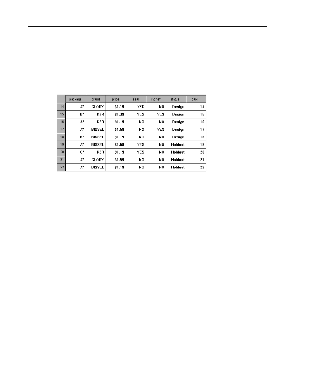
Figure 2-1 shows the Data Editor, displaying the orthogonal design for the carpet­cleaner example. The factors are displ ayed as the variables an d the cases created by the
procedure. Each case in the Data Editor represents one case in the orthogonal design.

Figure 2-1

Orthogonal design for the carpet-cleaner example

By default, the minimum number of cases necessary for an orthogonal array is
generated. The procedure determines the number of cases that needs to be administered
to allow estimation of the utilities. You can also specify a minimum number of cases
to generate. You might want to do this because the default number of minimum cases
is too small to be useful, or because you have experi mental design consi derations t hat
require a certain minimum number of cases. In this example, a minimum of 18 cases
was specified.

In addition to the cases in the desi gn, you c an specify holdout cases. Holdout cases
are judged by the subjects but are not used by the conjoint analysis to es timate utilities.
They are used as a check on the validity of the estimated utilities. The holdout cases
are generated from another random plan, not the experimental orthogonal plan.
Holdout cases always appear after th e experimental cases, unless you sp ecify that they
are to be mixed randomly with the other cases.

The orthogonal plan is saved like any other data file f or use in display ing the design
as profiles for subjects, and in the conjoint analysis.

Notice that two additional variable s,
assigns a sequential number to each profile for your convenience.

card_ and status_, appear in the data file. Card_

Status_ indicates

whether a case is part of the experimental orthogonal design (the first 18 cases in
Figure 2-1 above), a holdout case (cases 19–22 in the example), or a simulation case.

Designing the Conjoint Study: Generating an Orthogonal Design

Entering Simulation Cases

After you have generated an orthogonal design, you can create simulation cases.
These are combinations that are not rated by the subjects but are included in the
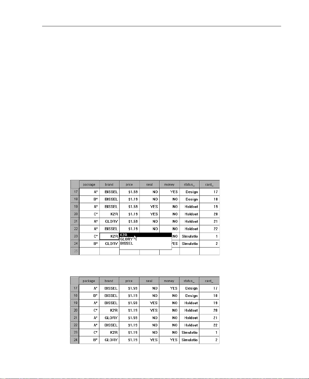
conjoint analysis, based on the ratings of the experimental profiles. Enter the cases
directly into the Data Editor, just as you would enter any data. The simplest way to
enter simulation cases is to use the value labels created when you generated the
experimental design, as displayed i n Figure 2- 2. To enter simulation cases using value
labels, be sure that
click the right mouse button to display the list of value labels for that variab le. Sel ect
the value label that you want to enter from the list. To enter the value into the cell,
double-click the lef t mouse button or press Ente
data into the Data Editor, see the SPSS Base User’s Guide. Figure 2-3 displays the
design for the carpet-cleaner study with two simulation cases added.

Figure 2-2

Entering values using value labels

Value Labels is selected on the Utilities menu. Select the cell, and

11

r. For more information about entering

Figure 2-3

Carpet-cleaner data including simulation cases

12

Chapter 2

What’s Next?

Thus far, we’ve generated an orthogonal plan of 18 cases, plus 4 holdouts and 2
simulations. To analyze the rankings of these profiles later, the plan must be saved. T o
save the file, select
any other data file. All factor names, factor levels, variable and value labels, the exact
factorial combination of each sequential case, the
and any data you have entered can be saved and used to display subject profiles and
can be used by a conjoint analysis.

Save Data from the File menu, and save the file just as you would

How to Obtain an Orthogonal Design

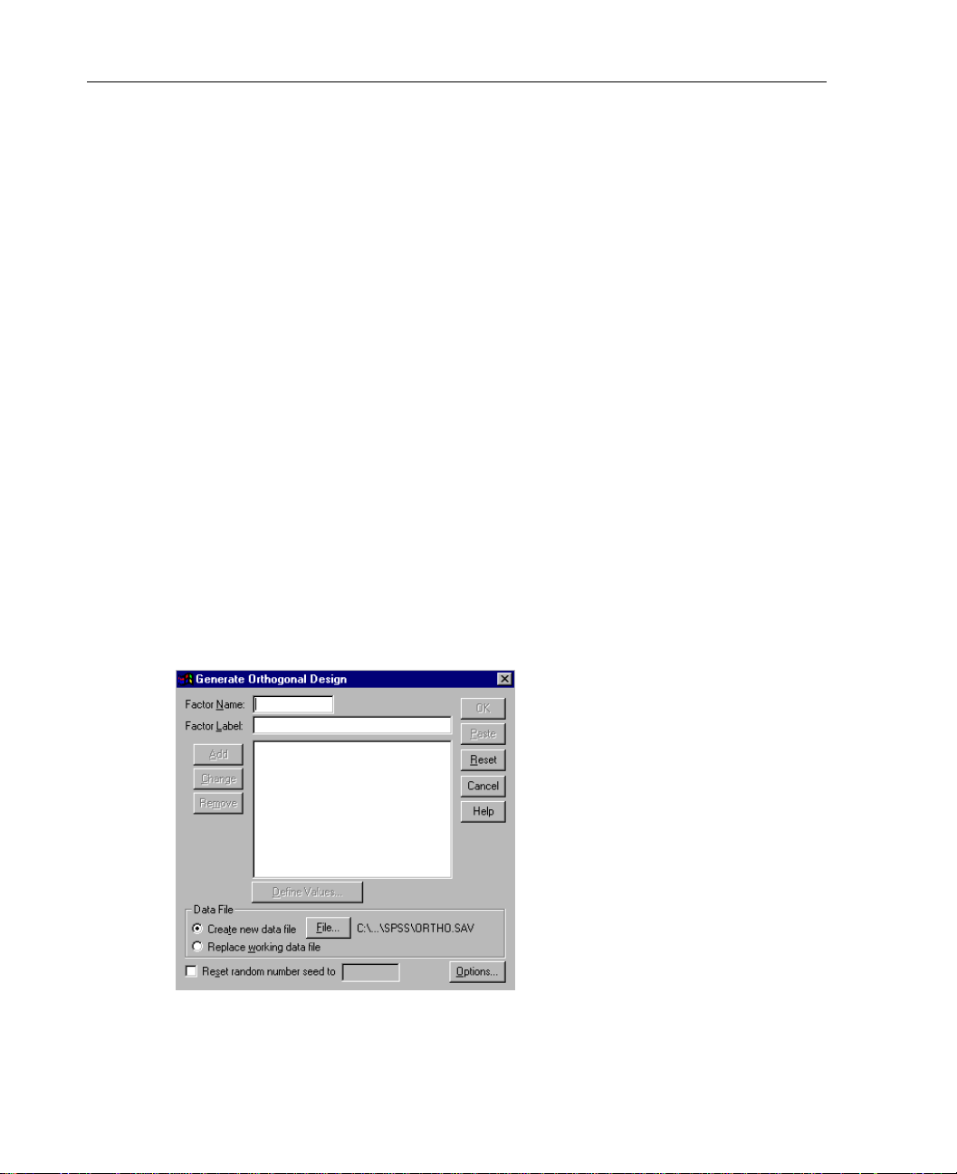
The Generate Orthogonal Design procedure generates a data file containing an
orthogonal main-effects design that permits the statistical testing of several factors
without testing every combination of factor levels. This design can be displayed with
the Display Design procedure, and t he data file may be used by other S PSS procedures,
such as Conjoint.

card_ variable, the status_ variable,

Figure 2-4

Generate Orthogonal Design dialog box

13

Designing the Conjoint Study: Generating an Orthogonal Design

 To obtain an orthogonal design, from the menus choose:

Data

Orthogonal Design 

Generate...

This opens the Generate Orthogonal Design dialog box, as shown in Figure 2-4.

 Define at least one factor. Enter a name for Factor Name. Factor names can be any

valid SPSS variable name, except

status_ or card_. You can also assign an optional

factor label.

 Click Add to add the factor name and an optional label. To delete a factor, select it in

the list and click
click

Change.

 Define values for the factors. (See “Define Values” on p. 15.)

Remove. To modify a factor name or label, select it in the list and then

Data File. Allows you to control the destination of the orthogonal desig n. Y ou can ei ther

create a new data file containing the ortho gonal desi gn, or you can replac e the current
working data file.

 Create new data file. Creates a new data file containing the factors and cases

generated by the plan. By default, this dat a f ile is named
to the current directory. Click

File to specify a different name and destination for

ortho.sav, and it is saved

the file.

 Replace working data file. Replaces the workin g data file with the generated plan.

You can choose to reset the random number seed.

 Reset random number seed to. Resets the random number seed to the specified

value. The seed can be any integer value from 0 through 2,000,000,000. Within a
session, SPSS uses a different seed each time you generate a set of random
numbers, producing different results. If you want to duplicate the same random
numbers, you should set the seed value before you generate your first design, and
reset the seed to the same value each subsequent time you generate the design.

To define values and value labels for a factor or factors, select the factor or factors in
the list and then click

Options to specify the minimum number of cases in the orthogonal design and

Click

Define Values in the main dialog box.

to select holdout cases.

14

Chapter 2

Output File Specification

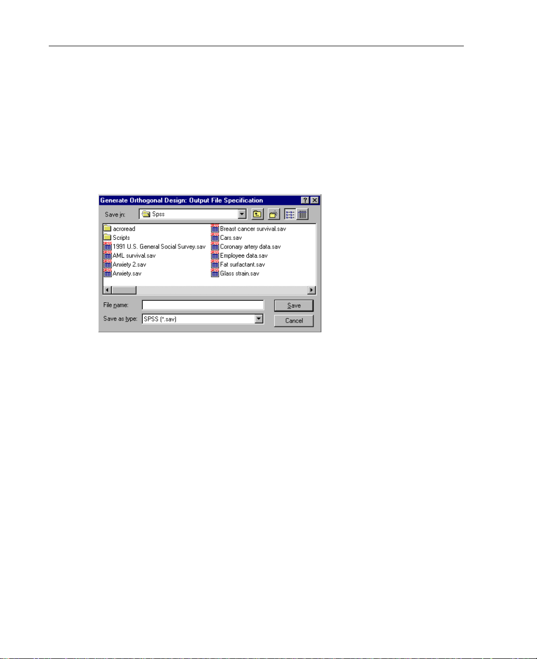
The Generate Orthogonal Design Output File Specification dialog box allows you to
specify a destination file for the orthogonal design. Figure 2-5 shows the Generate
Orthogonal Design Output File Specification dialog box for Windows.

Figure 2-5

Generate Orthogonal Design Output File Specification dialog box (Windows version)

See the SPSS Base User’s Guide for information on how to save data files.

Define Values

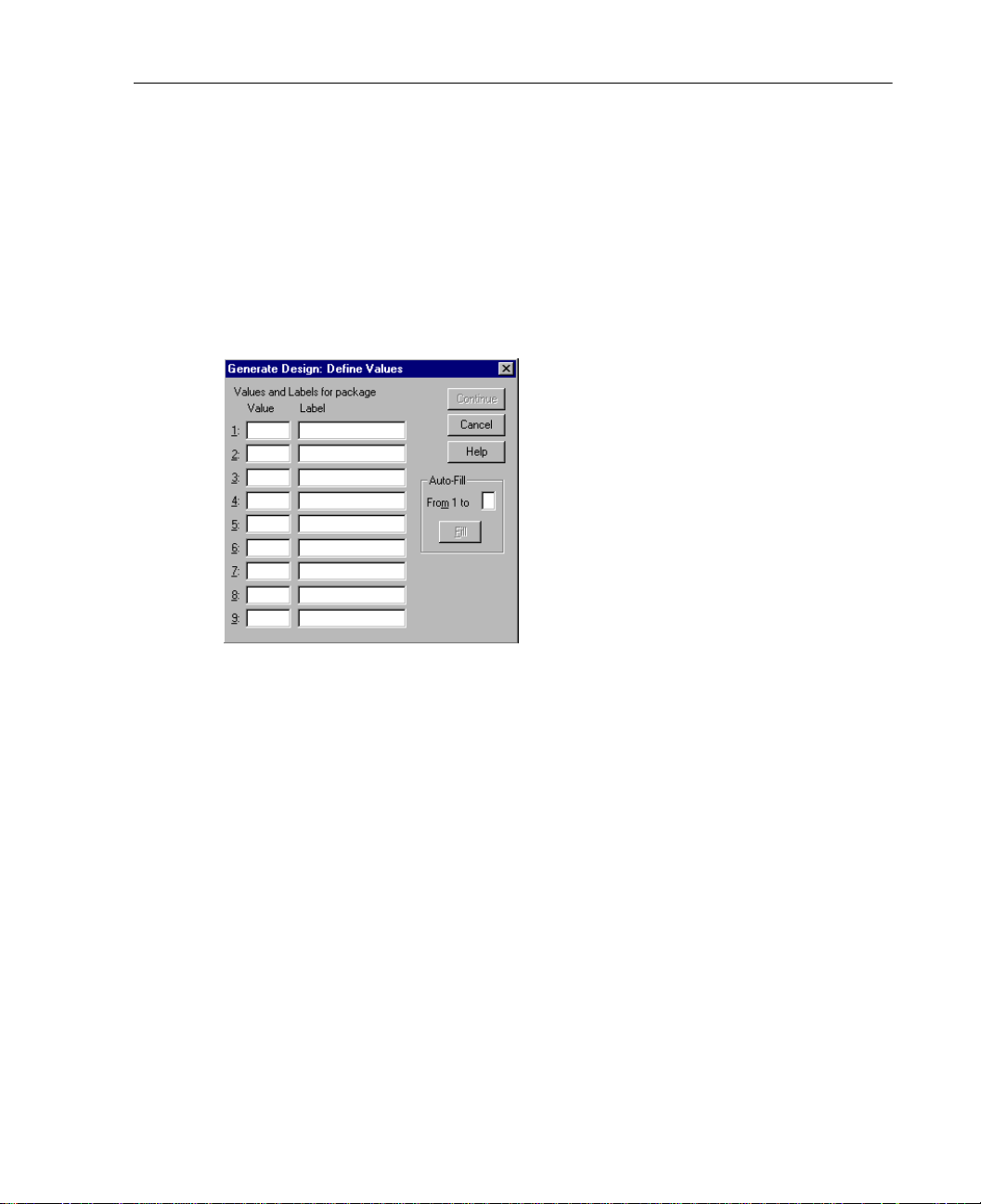
You must assign values to each level of the selected factor or factors. Select one or
more factors and click
dialog box, as shown in Figure 2-6.

Figure 2-6

Generate Design Define Values dialog box

15

Designing the Conjoint Study: Generating an Orthogonal Design

Define Values. This opens the Generate Design Define Values

If you have selected one factor, the factor name will be displayed after

Labels for
for Selected Variables

labels. Enter the label names for

. If you have selected multiple factors, the text displays Values and Labels

.

Enter each value of the factor for

Value. You can elect to give the values descriptive

Label. If you do not assign labe ls to the values, labels

Values and

that correspond to the values are automatically assi gned (that is, a va lue of 1 is assigned
a label of 1, a value of 3 is assigned a label of 3, and so on).

Auto-Fill. Allows you to automatic ally fill the Value boxes with consecutive values

beginning with 1. Enter the maximum value for

From 1 to, and click Fill t o fi ll in the

values.

16

Chapter 2

Options

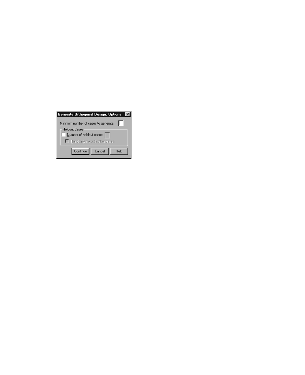
The Generate Orthogon al Design Option s dialog bo x, shown in Figu re 2-7, all ows you
to specify a minimum number of cases to be include d in the orthogonal design and to
select holdout cases.

Figure 2-7

Generate Orthogonal Design Options dialog box

Minimum number of cases to generate. Specifies a minimum number of cases for the

plan. Select a positive integer less than or equal to the total number of cases that can
be formed from all possible combi nati ons of t he fact or le vel s. If you do not explicitly
specify the minimum number of cases to generate, the minimum number of cases
necessary for the orthogonal plan is generated. If the Orthoplan procedure cannot
generate at least the number of profiles requested for the minimum, it will generate the
largest number it can that fits the specified factors and le vels. Note that the design does
not necessarily include exactly the number of specified cases, but rather the smallest
possible number of cases in the orthogonal design using this value as a minimum.

Holdout Cases. You can define holdout cases that are rated by subjects but are not

included in the conjoint analysis.

 Number of holdout cases. Creates holdout cases in addition to the regular plan cases.

Holdout cases are judged by the subjects, but are not used when the Conjoint
procedure estimates utilities. You can specify any positive integer less than or
equal to the total number of cases that can be formed from all possible
combinations of factor levels. If you do not specify a holdout value, no holdout
cases are produced. Holdout cases are generated from anothe r random plan, not the
main-effects experimental plan. The holdout cases do not duplicate the
experimental profiles or each other.

 Randomly mix with other cases. Randomly mixes holdout cases with the

experimental cases. When this option is deselected, holdout cases appear
separately after the experimental cases in the file.

Designing the Conjoint Study: Generating an Orthogonal Design

Additional Features Available with Command Syntax

You can customize your orthogonal design if you paste your selections into a syntax
window and edit the re sulting
User’s Guide). SPSS command language also allows you to:

 Append the orthogonal de sign to the existing working dat a file, rather than creati ng

a new file.

 Specify simulation cases b efore gener ating t he orthogon al design , rather than afte r

the design has been created.

See the Syntax Reference section of this manual for command syntax rules and for
complete

ORTHOPLAN command syntax.

ORTHOPLAN command syntax (see the SPSS Base

17

Chapter

3

Creating the Experimental Stimuli: Displaying the Design

As described in Chapter 1, once you h ave your d esig n plan, you need to put each ful l
concept on a separate p rofile to administer to respondents. Each case in the orthogonal
design is displayed as a profile.

You can display subject pr ofil es easily. Profiles can be c usto mize d t o l ook as you
want them to look. Each concept can be produced as a se parate page and yo u can add
titles and/or footers at the top or bottom of each profile. You can also control spacing
so that graphics or pictorial stimuli can be added to the profiles.

Creating the Carpet-Cleaner Profiles

Before printing each profile on a se parate page, you might want to look at them either
online or on a printo ut in a more condensed fo rmat. Figure 3-1 displ ays the orthogonal
design generated in Chapter 2. Th is format is an easy way t o get an idea of wha t your
output will look like so t hat yo u can go back and make any additions or changes that
you want. You can also view your plan file by displaying it in the Data Editor.

19

20

Chapter 3

Figure 3-1

Profiles displayed in listing format

Title: A Carpet Cleaner
Card 1
brand name Glory
moneyback guarantee? no
package design A*
price $1.39
Good Housekeeping Seal? yes
Card 2
brand name K2R
moneyback guarantee? no
package design B*
price $1.19
Good Housekeeping Seal? no
...

Card 22 (Holdout)
brand name Bissell
moneyback guarantee? no
package design A*
price $1.19
Good Housekeeping Seal? no

Simulations:

Card 1
brand name K2R
moneyback guarantee? no
package design C*
price $1.19
Good Housekeeping Seal? no
Card 2
brand name Glory
moneyback guarantee? yes
package design B*
price $1.19
Good Housekeeping Seal? yes

21

Creating the Experimental Stimuli: Displaying the Design

Once you’re sure that the output looks satisfactory, you can display the design again,
this time with each profile on a separate page. Figure 3-2 shows the design displayed
in this format for the first two profiles.

Figure 3-2

Profiles displayed in single-profile format

A New Carpet Cleaner

brand name Glory
moneyback guarantee? no
package design A*
price $1.39
Good Housekeeping Seal? yes

*Package Designs:

A New Carpet Cleaner

brand name K2R
moneyback guarantee? no
package design B*
price $1.19
Good Housekeeping Seal? no

*Package Designs:

Note that profiles that ar e ra ted by the sub jects, inclu ding h oldout p rofil es, ar e print ed
in single-profile format. Simulation profiles, however, are printed only in listing
format, since these profiles never actually get rated.

The last line on e ach pr ofil e in Figu re 3 -2 i s

*Package Designs. Using a footer like

this allows you to reserve space to manually add pictorial representations. Pictures can
sometimes be a very important part of conveying the concept to the subject. In this
example, any verbal description of the different package designs falls short when
compared to the drawings.

When you administer these profiles to subjects, you need to know the number of the
profile to accurately record and analyze the data. This number is the sequential number
of the profile as it appears in the plan file. You can either put this number on the front
of the profile as part of the title or footer, or you can simply write the number on the back
of each profile yourself. It is important to be able to easily identify each profile’s
position in the plan file so that the conjoint analysis knows what factor levels are on what
profiles by matching the order of the ranking or scores with the order in the plan file.

22

Chapter 3

How to Display an Orthogonal Design

The Display Design procedure allows you to print an experimental design. You can
print the desig n in either a rough-dra ft list ing format or as profiles that you can present
to subjects in a conjoint study. This procedure can display designs created with the
Generate Orthogonal Design procedur e or any designs displayed i n a working data file.

 To display an orthogonal design, from the menus choose:

Data

Orthogonal Design 

Display...

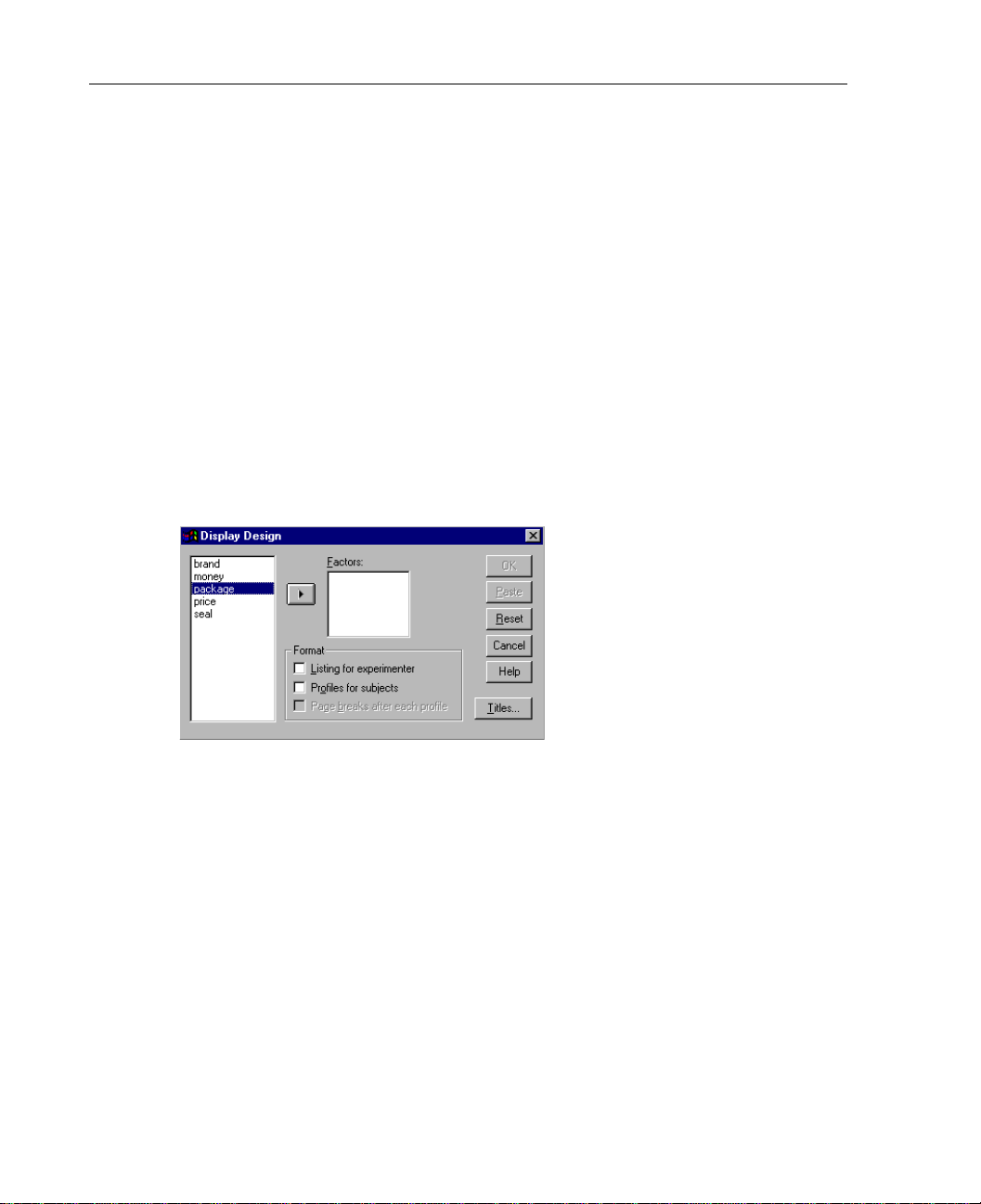
This displays the Display Design dialog box, as shown in Figure 3-3.

Figure 3-3
Display Design dialog box

 Move one or more factors into the Factors list.

 Select a format for disp laying the profiles in the o utput.

 You can choose to define headers and footers for the profiles. (See “How to Display

Orthogonal Design Titles” on p. 23.)

Format. You can choose one or more of the following format options:

 Listing for experimenter. Displays the design in a draft format that differentiates

holdout profiles from ex perimental p rofiles and lists si mulation pr ofiles separately
following the experimental and holdout profiles.

Creating the Experimental Stimuli: Displaying the Design

 Profiles for subjects. Produces profiles that can be presented to subjects. This

format does not differentiate holdout profiles and does not produce simulation
profiles.

 Page breaks after each profile. Begins each new profile on a new page.

How to Display Orthogonal Design Titles

You can define text that appears at either the top or t he bottom of th e output or profi le.
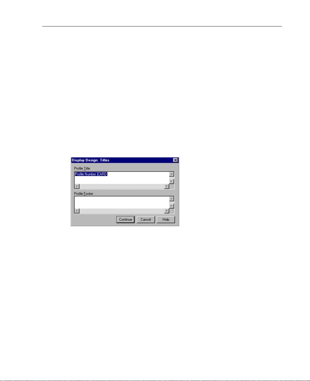
T o define titles, click
in Figure 3-4.

Figure 3-4

Display Design Titles dialog box

Titles. This opens the Display Design T itles dialog box, as shown

23

Profile Title. Enter a profile title up to 80 characters long. Titles app ear at the top of the

output if you have se lected
if you have selected
displays the profile number at the top of each profile. The variable

Listing for experimenter, and at the top of each new profile

Profiles for subjects in the main dialog box. The default title

)CARD prints the

profile number and is available only if you are displaying profiles for subjects.

Profile Footer. Enter a profile footer up to 80 characters long. Footers appear at the

bottom of the output if you have selected
of each profile if you have selected
are displaying profiles for subjects, you can enter

Listing for experimenter and at the bottom

Profiles for subjects in the main dialog box. If you

)CARD to print the profile number

in the footer.

24

Chapter 3

Additional Features Available with Command Syntax

You can customize your display design if you paste your selections into a syntax
window and edit the resulting
User’s Guide). SPSS command language also allows you to:

 Write profiles for subjects to an external file (using the OUTFILE subcommand).

See the Syntax Reference section of this manual for command syntax rules and for
complete

PLANCARDS command syntax.

PLANCARDS command syntax (see the SPSS Base

Analyzing Preferences: Using the Conjoint Procedure

In Chapter 2 and Chapter 3, we generated an orthogonal design and printed the
experimental stimuli for a full-concept conjoint analysis study. In this chapter, we’ll
see how the data are collected and analyzed.

Chapter

4

Collecting the Data

Since there is typically a great deal of between-subject variati on in preferences, much
of conjoint analysis focuses on the sin gle subject. To generalize the results, a random
sample of subjects from the target population is selected so that group results can be
examined.

The size of the sample in co njoint studi es varies greatly. Cattin and Wit tink (1982)
report that the sample size in commer cial conjoi nt studies usually r anges from 100 t o
1000, with 300 to 550 the most typical range. Akaah and Korgaonkar (1988) report
that smaller sample sizes (less than 100) are typical. As always, the sample size should
be large enough to ensure reliability.

Once the sample is chosen, the researcher administers the set of full-concep t cards,
or profiles, to each respondent. The Conjoint procedure allows t hree methods o f data
recording. In the first method, subjects are asked to assign a preference score to each
profile. This kind of method is typical when a Likert scale is used or when the subj ects
are asked to assign a number from 1 to 100 to indicate preference. In the second
method, subjects are asked to assign a rank to ea ch profil e ran ging from 1 to t he t otal
number of profiles. In the third method, subjects are asked to sort the profiles i n terms
of preference. With this last method, the researche r records the prof ile numbers in the
order given by each subject.

25

26

Chapter 4

Analyzing Carpet-Cleaner Preference

Once the data are collected, the Conjoint procedure c an be used to estimate part-worths
for each factor level. These part-worth scores indicate the influence o f each factor level
on the respondent’s preference for a particular combin ation. They are comput ed by the
procedure through a set of regressions of the ranki ngs or scores on the profiles. Since
they are all expressed in a common unit, the part-worth scores can be added together
to give the total utility of a combination. To be useful, the total utilities should be
highly correlated with the observed preference data.

In this release of SPSS, a graphical user interface is not yet available for the Conjoint
procedure. Examples in this chapter demonstrate conjoint analysis using SPSS
command syntax. Figure 4-1 shows the set of SPSS commands for analyzing the carpet­cleaner data. Preference data for 10 subjects are defined. In this example, the sequence
method of data collection was used. That is, subjects were asked to sort the profiles from
the most to the least preferred. Subject 1, for example, liked profile 13 most of all, so 13
is the first data point. Once again, this shows why it is important for the preference data
to match the sequential order of the profiles in the plan file. The
will look at the 13th profile in that plan file for information on what factor levels subject
1 liked best. The
subcommand indicates that the preference data are located in the working data file.

PLAN subcommand identifies the plan system file, and the DATA

CONJOINT command

Figure 4-1

CONJOINT command for carpet-cleaner example

DATA LIST FREE /ID PREF1 TO PREF22.

BEGIN DATA

01 13 15 01 20 14 07 11 19 03 10 17 08 05 09 06 12 04 21 18 02 22 16

02 15 07 18 02 12 03 11 20 16 21 06 22 08 17 19 01 14 04 09 05 10 13

03 02 18 14 16 22 13 20 10 15 03 01 06 09 05 07 12 19 08 17 21 11 04

04 13 10 20 14 02 18 16 22 15 03 01 09 05 06 08 17 11 07 19 04 12 21

05 13 18 02 10 20 15 09 05 03 07 11 04 12 22 14 16 01 06 19 21 17 08

06 15 02 03 12 18 07 20 10 11 04 09 05 13 16 14 22 08 06 01 21 19 17

07 13 07 15 18 02 03 10 20 14 11 19 17 12 01 09 05 04 06 08 16 21 22

08 15 07 13 04 06 16 08 22 05 09 21 18 10 03 02 20 14 11 17 19 01 12

09 20 09 10 11 04 05 13 15 02 03 12 18 07 01 21 14 16 22 08 06 17 19

10 08 21 19 17 04 11 12 07 01 06 09 05 03 15 14 16 22 20 10 13 02 18

END DATA.

CONJOINT PLAN=’ CP LAN.SAV’

/DATA=* /SEQUENC E= PREF1 TO PREF22 /SUBJE CT=ID

/FACTORS=PACKA GE BRAND (DISCRETE) PRIC E (LINEAR LESS)

SEAL (LINEAR MORE) MONEY (LINEAR MORE)

/PRINT=ALL /UTILITY=’RUGUTIL.SAV’.

SAVE OUTFILE=’RUGRANKS.SAV’.

The

FACTORS subcommand specifies a model describing the expected relationship

between the preference data and the factor levels. The factors specified refer to
variables defined in the plan system file named on the

PLAN subcommand.

27

Analyzing Preferences: Using the Conjoint Procedure

Four different kinds of models can be specified on FACTORS: DISCRETE, LINEAR,

IDEAL, and ANTIIDEAL. DISCRETE is u sed when the factor levels are categorical and no

assumption is made about the relationship between the levels and the data.
assumed by default if you don’t include a model specifi cati on on

FACTORS. LINEAR

DISCRETE is

indicates that the data are expected to be linearly related to the factor. Price is typically
linear, since consumers frequently prefer lower prices. You can also specify keywords

MORE or LESS after DISCRETE or LINEAR to indicate an expected direction of the

relationship.

IDEAL and ANTIIDEAL are quadratic function models. The IDEAL model has

an ideal factor level, and distance from this ideal point is associated with decreasing
preference. When plotted, the

ANTIIDEAL is very similar. The only difference is that preference increases with distance

IDEAL function usually has an upside-down U shape.

from the point, so this point is hypothesized t o be t he worst level of the factor. When
plotted, the

For our example, the

and a

price, since it is expected that the higher the price, the lower the preference. For seal

ANTIIDEAL function is usually U-shaped.

DISCRETE model was specified for factors package and brand,

LINEAR model for factors price, seal, and money. LESS was specified for factor

and money, the levels were ordered No first and Yes second in the plan file. Thus,

MORE is used for these factors, since it is expected that Yes (the higher level) will be

associated with higher preference.

Separate output for each subject as well as the group is obtained by using the

SUBJECT subcommand. Figure 4-2 shows the output for the first subject. The output

shows the utility (part-worth) scores and their st andard errors for each factor level. As
mentioned previously, by adding these values, the total utility of a specific
combination can be computed.

For example, the total util ity of a cleaner with packag e design B*, bran d K2R, price

$1.19, and no seal of approval or money-back guarantee is:

utility(package B*) + utility(K2R) + utility($1.19) + utility(no seal)
+ utility(no mo ney-back) + constant

or:

0.6667–()1.3333–()2.4792+ + 9.000 5.0000 12.062–()+ + + 2.4172=

If the cleaner had package design C*, brand Bissell, price of $1.59, a seal of approval,
and a money-back guarantee, the total utility would be:

0.6667 0.3333 3.3125 18.0000 10.0000 12.062–()+ + + + + 20.2505=

28

Chapter 4

The total utilities should correspond closely to the observed data. For RANK and

SEQUENCE data, however, remember that the relationship is reversed. Low values

indicate high preference and will therefore produce high utilities. Conversely, high
values indicate low preference and yield low utilities.

The total utilities might be a little off from the observed data due to the lack of fit. The
standard error for each utility is one indication of how well the model fits that particular
subject’s data. Looking at subject 1, we can see that the standard errors for

price are

relatively high, and thus a linear model was probably not best for this factor for this subject.

Figure 4-2

CONJOINT results for subject 1

SUBJECT NAME: 1.00

Importance Utility(s.e.) Factor ** Reversed ( 1 reversal )

++ PACKAGE package design

7.21 II .0000( .6303) I A*
++ -.6667( .6303) I B*
I .6667( .6303) I C*
I
+--+ BRAND brand name

12.61 I I -1.3333( .6303) I K2R
+--+ 1.0000( .6303) I Glory
I .3333( .6303) I Bissell
I
++ PRICE ** price

4.50 II 2.4792(3.2476) I- $1.19
++ 2.8958(3.7934) I- $1.39
I 3.3125(4.3392) I- $1.59
I B = 2.0833(2.7291)
I
+---------+ SEAL Good Housekeeping Seal?
I48.65 I 9.0000( .9454) I-- no
+---------+ 18.0000(1.8908) I---- yes
I B = 9.0000( .9454)
I
+-----+ MONEY moneyback guarantee?
I27.03I 5.0000( .9454) I- no
+-----+ 10.0000(1.8908) I-- yes
I B = 5.0000( .9454)
I

-12.062(4.2150) CONSTANT

Pearson’s R = .962 Significance = .0000

Kendall’s tau = .869 Significance = .0000
Kendall’s tau = .667 for 4 holdouts Significance = .0871

Simulation results:

Card: 1 2

Score: 3.8 18.8

Some additional results for each factor in the CONJOINT output are the value of B, the
linear regression coefficient o r sl ope for linear and quadratic models, and the value of
C, the quadratic term for
predicted score can be calculated by multiplying the factor value by B. For quadratic
models, the predicted sc ore can be calculate d by multiplying th e factor value by B, and
adding that value to the product of C and the square of the factor value.

For

IDEAL and ANTIIDEAL models, the value of the ideal point is also displayed.

Relative Importance

Since the part-worth scores are expressed on a common scale, the factors can be
compared by looking at the ranges (highest–lowest ) of these util ities.
these ranges to compute importance scores for each factor. These are listed in the
leftmost column of Figure 4-2 along with a bar chart to give you an idea of how the
factors compare.

The importance scores are computed by taking the utility range for the particular

factor and dividing it by the sum of all the uti lity ranges. Fr om Figure 4- 2, we can see
that subject 1 thought a Good Ho usekeeping seal was ver y important (48.6 5), whereas
the price was not (4.50). By using the importance scores, the total utility of any
combination, even ones not rated by subjects, can be predicted.

Notice also that there are two asterisks (**) displayed next to
that the direction speci f ie d (
expensive cleaners. “Reversals” are marked in this way when ever a specified

LESS direction is not observed, or when a predicted IDEAL or ANTIIDEAL function is

reversed.

The Pearson’s R and Kendall’s tau statistics displayed at the bottom of each
subject’s output is another indication of how well the model fits the data. They are
correlations between the observed and estimated preferences. As such, these
coefficients should always be very high.

In many conjoint analyses, the number of parameters is close to the number of
profiles rated, which will artificially inflate the correlation between observed and
estimated scores. In these cases, the correlation between observed and estimated scores
for the holdout profiles may giv e a better indi cation of the fi t of the model, since these
profiles were not used to estimate scores. Keep in mind, however, that holdouts will
always produce lower correlation coefficients.

29

Analyzing Preferences: Using the Conjoint Procedure

IDEAL and ANTIIDEAL models. For LINEAR models, the

CONJOINT uses

price. This indicates

LESS) was not observed. This subject preferred the more

MORE or

30

Chapter 4

The Holdouts and Simulations

Four of the profiles in the carpet-cleaner example were holdout profiles. This means
that they were rated by the subjects but that the Conjoint procedure did not use them
when estimating the utilities. Instead, the Conjoint procedure computes correlations
between the observed and predicted rank orders for these profiles as a check on the
validity of the u tilities.

There were two other combinations in the plan file, the simulations. These
combinations were never printed by
Results for these two hypothetical profiles are estimated by the Conjoint procedure
based on the ratings of the experimental profiles. As can be seen from the bottom of
Figure 4-2,
profile for each subject. With preference scores estimated by
score, the greater the preference, regardless of how the observed data were scaled.
Thus, for subject 1, we see that simulation profile 1 w ould not have been rated
favorably but simulation profile 2 would have been rated very favorably.

Simulations do not have to be entered during the same session as the experimental
profiles, nor do they have to already be part of the accessed plan file, as they were in
this example. Adding a saved plan file to some n ew simulations and then accessing the
preference data file, as i n Figure 4-3, produces simul ated judgments of the new profi les
by using the part-worths estimated from the rankings of the experimental profiles.
Keyword
the simulation analysis. The commands in Figure 4-3 reproduce the same results for
the two simulation profiles previously analyzed.

CONJOINT computes an estimated preference score for each simulation

SIMULATION is available on the PRINT subcommand to limit output to just

PLANCARDS or administered to the subjects.

CONJOINT, the higher the

Figure 4-3

Running future simulations

DATA LIST FREE /PAC KAG E BRAND PRICE SEAL MONE Y CARD_.

BEGIN DATA

3 1 1.19 1 1 1

2 2 1.19 2 2 2

END DATA.

COMPUTE STATUS_=2.

ADD FILES FILE=’CPLAN.SAV’ /FILE=*.

CONJOINT PLAN=* /DA TA=’RUGRANKS.SAV ’

/SEQUENCE=PREF1 TO PREF22

/SUBJECT=ID

/FACTORS=PACKA GE BRAND (DISCRETE) PRIC E (LINEAR LESS)

SEAL (LINEAR MORE) MONEY (LINEAR MORE)

/PRINT=SIMULATION.

Subfile Summary

When using the SUBJECT subcommand, you get the results discussed in this chapter
for each subject as well as averaged results for the whole group. Figure 4-4 shows the
group results for the carpet-cleaner study. Across all subjects in this study, package
design was clearly the most important factor.

Figure 4-4

Group results from CONJOINT

SUBFILE SUMMARY
Averaged
Importance Utility Factor
+---------+ PACKAGE package design
I35.63 I -2.2333 -I A*
+---------+ 1.8667 I- B*
I .3667 I C*
I
+---+ BRAND brand name

14.91 I I .3667 I K2R
+---+ -.3500 I Glory
I -.0167 I Bissell
I
+-------+ PRICE price
I29.41 I -6.5946 ---I $1.19
+-------+ -7.7029 ---I $1.39
I -8.8113 ----I $1.59
I B = -5.5417
I
+--+ SEAL Good Housekeeping Seal?

11.17 I I 2.0000 I- no
+--+ 4.0000 I-- yes
I B = 2.0000
I
+-+ MONEY moneyback guarantee?

8.87 I I 1.2500 I- no
+-+ 2.5000 I- yes
I B = 1.2500
I

12.8696 CONSTANT

31

Analyzing Preferences: Using the Conjoint Procedure

Pearson’s R = .982 Significance = .0000
Kendall’s tau = .892 Significance = .0000
Kendall’s tau = .667 for 4 holdouts Significance = .0871

Simulation results:
Card: 1 2
Score: 10.3 14.3

32

Chapter 4

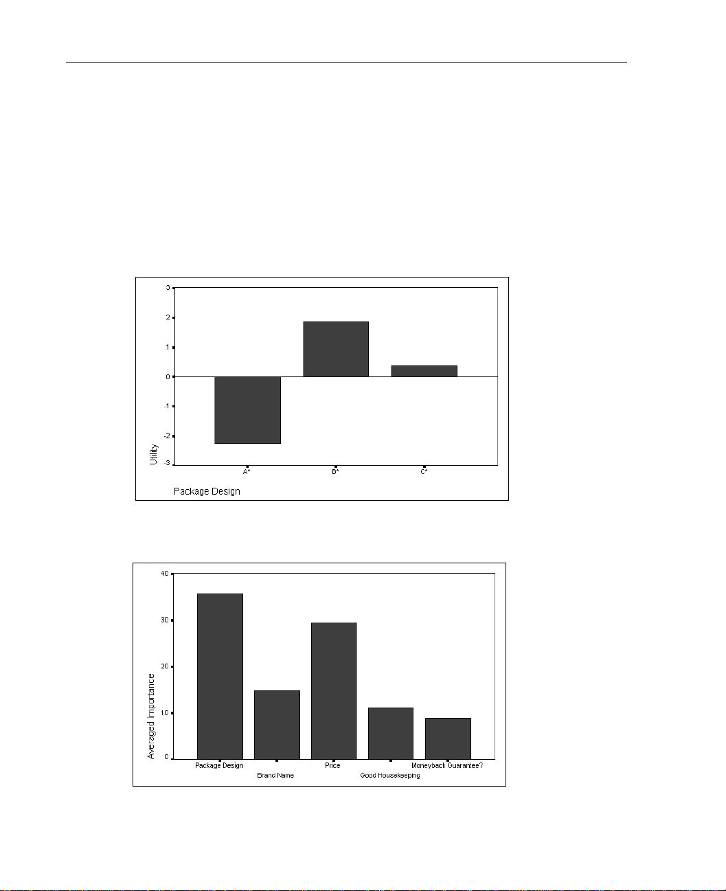
The PLOT subcommand provides another way for you to look at the group re sults. The

SUMMARY keyword produces one bar chart for every variable, showing the utility

scores for each category of that variable, and a chart showing the summary importance
scores for each variable. You can also request charts of the utility and importance
scores by subjects with the
utilities for

Figure 4-5

Summary utilities for package

package and Figure 4-6 shows the importance summary.

SUBJECT keyword. Figure 4-5 displays the summary

Figure 4-6

Importance summary

33

Analyzing Preferences: Using the Conjoint Procedure

Figure 4-7 shows some additional group statistics. The Conjoint procedure displays
summary results on reversals and simulations. The simulation summary gives the
probabilities of choosing particular simulation profiles as the most preferred profiles
under three different probability-of-choice models. The maximum utility model is
simply the probability o f choosing a profi le as the most pref erred. The BTL (Bradley-
Terry-Luce) model computes the probability of choosing a profile as the most
preferred by dividing the profile’s utility by the sum of all the simulation total utilities.
The logit model is similar to BTL but uses the natural log of the utilities instead of the
utilities. Across the 10 subjects in this study , all three models indicated that simulation
profile 2 would be more preferred.

Figure 4-7

Reversal and simulation summary

Reversal Summary:
2 subjects had 2 reversals
3 subjects had 1 reversals

Reversals by factor:
PRICE 3
MONEY 2
SEAL 2
BRAND 0
PACKAGE 0

Reversal index:
Page Reversals Subject
49 1 1.00
50 2 2.00
51 0 3.00
52 0 4.00
53 0 5.00
54 1 6.00
55 0 7.00
56 0 8.00
57 1 9.00
58 2 10.00

Simulation Summary (10 subjects/ 10 subjects with non-negative scores)
Card Max Utility BTL Logit
1 30.00% 43.07% 30.92%
2 70.00 56.93 69.08

34

Chapter 4

The Utility File

The UTILITY subcommand, shown in Figure 4-1, writes out an SPSS data file
containing for each subject the utilities for
functions for

LINEAR, IDEAL, and ANTIIDEAL factors (labeled B and C in the output),

DISCRETE factors, the slope and quadratic

the regression constant, and the estimat ed preference scores. Thes e values can then be
used in further analyses or for making additional plots and graphs with other
procedures.

How to Obtain a Conjoint Analysis

Conjoint analysis is a technique for measuring people’s preferences of stimuli with
multiple attributes. It provides a means of determining which combinations of
attributes are most preferred , whic h indi vidual at tributes most influenc e preference of
the total item, and the relative importance of each factor . Conjo int analysis also allows
you to predict the ef fects of fact or le vel co mbinat ions that we re not actual ly p resented
in the experiment.

In this release of SPSS, a graphical user interface is not yet available for the
Conjoint procedure. To obtain a conjoint analysis, you must enter SPSS commands
into a syntax window, and then run them. To obtain a conjoint analysis:

 From the menus choose:

File

New 

SPSS Syntax...

This opens an SPSS syntax window.

 Enter the commands that you want to run in the syntax window.

 Select the commands that you want to run, and then click the Run Syntax too l ( ) on

the toolbar.

See the SPSS Base User’s Guide for more informat ion about ru nning commands in
syntax windows. See the Syntax Refe rence section of this manual for comman d syntax
rules and for complete

CONJOINT command syntax.

Minimum Specifications

The minimum specifications for a Conjoint analysis include the specification of two
files—a data file and a plan file—and the specification of how data were recorded.
Files are specified with the
recording is specified with the
following syntax shows a minimal specification for a conjoint analysis of the carpet­cleaner study:

CONJOINT PLAN=* /DATA=’RUGRANKS.SAV’
/SEQUENCE=PRE F1 TO PREF 22.

Specifying the Files

The Conjoint procedure requires two files—a plan file and a da ta file. The plan file can
be created using the Orthoplan procedure, as in th e example shown in Figure 4-1, or it
can be entered into the Data Editor like any data file. If only a plan file or a data file is
specified, the
file as the other. The plan file is specified with the
is specified with the

For example, the command

CONJOINT PLAN=’CPLAN.SAV’ /DATA=’RUGRANKS.SAV’

specifies that the plan file to be used in the conjoint analy sis is cplan.sav, and the data
file to be used in the analysis is
working data file as the data file, specify:

CONJOINT PLAN=’CPLAN.SAV’ /DATA=*

The asterisk (*) indicates that the working data file should be used as the data file. You
can also eliminate the
automatically be used as the data file. Si milarly, you can specify a data file and use the
current working data file as the plan file. For example:

CONJOINT PLAN=* /DATA=’RUGRANKS.SAV’

CONJOINT command reads the specified file and uses the working data

35

Analyzing Preferences: Using the Conjoint Procedure

PLAN and DATA subcommands. The method of data

SEQUENCE/RANK/SCORE subcommands. The

PLAN subcommand, and the data file

DATA subcommand.

rugranks.sav. T o speci fy a plan file and use the current

DATA subcommand altogether, and the working data file will

Specifying How Data Were Recorded

You must specify the way in which preference data were recorded. Data can be
recorded in one of three ways: sequentially , as rankings, or as preference scores. These

36

Chapter 4

three methods are indicated by the SEQUENCE, RANK, and SCORE subcommands.
You must specify one, and only one, of these subcommands.

SEQUENCE Subcommand

The SEQUENCE subcommand indicates that data were recorded sequentially so that
each data point in the data file is a profile number, starting with the most preferred
profile and ending with t he least pr eferred profi le. Th is is h ow data are recor ded if t he
subject is asked to order the profiles from the most to the least preferred. The
researcher records which profile numb er was firs t, which pr ofi l e numbe r was second,
and so on. The data in the carpet- cleaner study were reco rded this way, as specified by
the following syntax:

CONJOINT PLAN=’CPLAN.SAV’

/DATA=* /SEQUENCE=PREF1 TO PREF22.

RANK Subcommand

The RANK subcommand indicates that each data point is a ranking, starting with the
ranking of profile 1, then the ranking of profile 2, and so on. This is how the data are
recorded if the subject is asked to assign a rank to each profile, ranging from 1 to n,
where n is the number of profiles. A lower rank implies greater preference. For
example, if the carpet-cleaner study had recorded data this way , and t he variables in the
study were named

CONJOINT PLAN=’CPLAN.SAV’

/DATA=* /RANK=RANK1 TO RANK22.

rank1 to rank22, it would be specified by the following syntax:

SCORE Subcommand

The SCORE subcommand indicate s that ea ch data point i s a preferenc e score assigned
to the profiles, starting with the score of profile 1, then the score of profile 2, and so
on. This type of data might be generated, for example, by asking subjects to assign a
number from 1 to 100 to show ho w much they lik ed the profile. A higher score impl ies
greater preference. For example, if the carpet-cleaner study had recorded data th is way,
and the variables in the study were na med
the following syntax:

CONJOINT PLAN=’CPLAN.SAV’

/DATA=* /SCORE =S CORE1 TO SCORE22.

score1 to score22, it would be specified by

Optional Specifications

In addition to the minimum required specifications, the CONJOINT command contains
optional subcommands that allow you to specify a subject identification variable,
specify a model for each factor, control analyses included in your output, and write a
utility file to a specified file.

SUBJECT Subcommand

The SUBJECT subcommand allows you to specify a subject identificatio n variab le . If
you do not specify a subject variable, the
come from one subject. In the carpet-cleaner study, the subject identification variable
is named

FACTOR Subcommand

The FACTOR subcommand allows you to specify the model describing the expected
relationship between factors and the rankings or scores. You can specify one of four
models:

id, as specified with the following syntax:

CONJOINT PLAN=CPLAN
/DATA=* /SEQUE NCE =PREF1 TO PREF22 /SUB JECT=ID

37

Analyzing Preferences: Using the Conjoint Procedure

CONJOINT com mand assumes that all data

DISCRETE. The DISCRETE model indicates that the factor levels are cate gorical and that

no assumption is made about the relationship between the factor and the scores or
ranks. If you do not speci fy a mod el for a factor,

LINEAR. The LINEAR model indicates an expected linear relationship between the

CONJOINT assumes a discrete model.

factor and the scores or ranks. You can specify the expected direction of the linear
relationship with the keywords
a factor are expected to be preferred, while

MORE and LESS. MORE indicates that hig her levels of

LESS indicates that lower levels of a factor

are expected to be preferred.

IDEAL. The IDEAL model indicates an expected quad ratic relationship with a decreasing

preference between the factor and the scores or ranks.

ANTIIDEAL. The ANTIIDEAL model indicates an expected qu adratic relationship wit h an

increasing preference between the fac tor and the scores or ran ks. In the c arpet-cleaner
study , the factors
model.

Price, seal, and money were all expe cted to have a linear relation ship to the

package and brand are categorical, and therefore assigned a discrete

38

Chapter 4

preference scores. Seal and money are expected to have a posi t iv e l ine ar r elationship,
as indicated by the keyword
relationship, as in di cat ed by the keyword
and

money, which correspond to the existence of a Good Housekeeping seal and a

money-back guarantee, preference is expected to increase. However, as price
increases, preference is expected to decrease. Following is the syntax specifying the
factors for the carpet-cleaner study:

/FACTORS=PACKAGE BRAND (DISCRETE) PRICE (LINEAR LESS) SEAL

(LINEAR MORE) MONEY (LINEAR MORE)

PRINT Subcommand

The PRINT subcommand allows you to control whether the output includes the analysis
of the experimental data , results of simulati on data, both, or none. If you do not spe cify
a

PRINT subcommand, the results of both t he experimental data and th e simulation data

are printed. The carpet-cleaner example included the results of both the experimental
and simulation data:

/PRINT=ALL

MORE, while price is expected to have a negative linear

LESS. That is, with the hi gher l ev els of seal

UTILITY Subcommand

The UTILITY subcommand writes a utility data file containing one case for each
subject. The utility file can be opened in the Data Editor and displayed or e dited like
any data file. The following syntax creates a utility file named

/UTILITY=’RUGUTIL.SAV’

rugutil.sav:

Syntax Reference

Introduction

This syntax reference guide describes the SPSS command language underlying SPSS
Conjoint. Most of the features of these commands are implemented in the dialog boxes and
can be used directly from the dialog boxes for
paste the syntax into a syntax window and edit it or build a command file, which you ca n
save and reuse. The features that are available only in command syntax are summarized fol­lowing the discussion of the dialog box interface in the corresponding chapter on each sta­tistical procedure. In contrast to the other procedures,
syntax.

A Few Useful Terms

All terms in the SPSS command language fall into one or more of the following categories:

Keyword. A word already defined by SPSS to identify a command, subcommand, or speci-

fication. Most keywords are, or resemble, common English words.

Command. A specific instruction that controls the execution of SPSS.
Subcommand. Additional instructions for SPSS commands. A command can contain more

than one subcommand, each with its own specifications.

Specifications. Instructions added to a command or subcommand. Specifications may

include subcommands, keywords, numbers, arithmetic operators, variable names, special
delimiters, and so forth.

Each command begins wit h a command keyword (which may contain more than one
word). The command keyword is followed by a t le ast one bl ank space an d t hen any addi­tional specifications. Each command ends with a command termi nator , which is a period.
For example:

Command

Subcommands

MEANS

TABLES=salnow BY jobcat
/CELLS=MEAN.

Command terminator

ORTHOPLAN and PLANCARDS. Or you can

CONJOINT is available only through

Specifications

Keywords

Syntax Diagrams

Each SPSS command described in this manual includes a syntax diagram that shows all of
the subcommands, keywords, and specifications allowed for that command. These syntax
diagrams are also available in the online Help system for easy reference when entering
commands in a syntax window. By remembering the following rules, you can use the
syntax diagram as a quick reference for any command:

41

42 Introduction

• Elements shown in all capital letters are keywords defined by SPSS to identify commands,

subcommands, functions, operators, a nd ot her spe cifica tion s.

• Elements in lower case describe specifications you supply.

• Elements in boldface type are defaults. A default indicated with two asterisks (**) is in

effect when the keyword is not specified. (Boldface is not used in the online Help system
syntax diagrams.)

• Parentheses, apostrophes, and quotation marks are required where indicated.

• Elements enclosed in square brackets (

• Braces (

{ }) indicate a choice among elements. You can specify any one of the elements

[]) are optional.

enclosed within the aligned braces.

• Ellipses indicate that an element can be repeated.

• Most abbreviations are obvious; for example,

varname stands for variable name and varlist

stands for a list of variables.

• The command terminator is not shown in the syntax diagrams.

Syntax Rules

Keep in mind the following simple rules when writing an d editing commands in a syntax
window:

• Each command must begin on a new line and end with a period.

• Subcommands are separated by slashes. The slash before the first subcommand in a

command is optional in most commands.

• SPSS keywords are not case-sensitive, and three-letter abbreviations can be used for most

keywords.

• Variable names must be spelled out in full.

• You can use as many lines as you want to specify a single comma nd. However, text

included within apostrophes or quotation marks must be contained on a single line.

• You can add space or break lines at almost any point where a single blank is allowed, such

as around slashes, parentheses, arithmetic operators, or between variable names.

• Each line of syntax cannot exceed 80 characters.

• The period must be used as the decimal indicator, regardless of your language settings-

LANG environment variable setting.

For example,

FREQUENCIES
VARIABLES=JOBCAT SEXRACE
/PERCENTILES=25 50 75
/BARCHART.

and

freq var=jobca t se xr ac e /p er ce nt =2 5 50 75 /b ar .

are both acceptable alternatives that generate the same re sults. The second example uses
three-letter abbreviations and lower case, and the command is on one line.

Introduction 43

Batch Mode and INCLUDE Files

If your SPSS commands are contained in a command file t hat is specified on the SPSS

INCLUDE command, For SPSS command files run in batch mode (see the SPSS Base System

User’s Guide) or via the SPSS

• Each command must begin in the first column of a new line.

• Continuation lines within a command must be indented at least one space.

• The period at the end of the command is optional.

If you generate command syntax by past ing di alo g box choi c es into a syn tax wi ndow, the for­mat of the commands is suitable for all modes of operation.

INCLUDE command, the syntax rules are slightly different:

CONJOINT

CONJOINT [PLAN={* }]
{file}

[/DATA={* }]
{file}

/{SEQUENCE}=varlist
{RANK }
{SCORE }

[/SUBJECT=variable]
[/FACTORS=varlist[’labels’] ([{DISCRETE[{MORE}]}]

{ {LESS} }
{LINEAR[{MORE}] }
{ {LESS} }
{IDEAL }
{ANTIIDEAL }
[values[’labels’]])]

varlist...

[/PRINT={ALL** } [SUMMARYONLY]]
{ANALYSIS }
{SIMULATION }
{NONE }

[/UTILITY=file]
[/PLOT={[SUMMARY] [SUBJECT] [ALL]}]

{[NONE**] }

**Default if subcommand or keyword is omitted.

Example:

CONJOINT PLAN=’CARPLAN.SAV’
/FACTORS=SPEED (LINEAR MORE) WARRANTY (DISCRETE MORE)
PRICE (LINEAR LESS ) SE AT S
/SUBJECT=SUBJ /RANK=RANK1 TO RANK15 /UTILITY=’UTIL.SAV’.

Overview

CONJOINT analyzes score or rank data from full-concept conjoint studies. A plan file

generated by
or ranked in terms of preference. A variety of continuous and discrete models is available
to estimate utilities for each individual subject and for the group. Simu lation estimates for
concepts not rated can also be computed.

ORTHOPLAN or entered by the user describes the set of full concepts scored

1

2CONJOINT

Options

Data Input. You can analyze data recorded as rankings of an ordered s et of profiles, or cards,

as the profile numbers arranged in rank order, or as preference scores of an ordere d set of
profiles.

Model Specification. You can specify how each factor is expected to be related to the scores or

ranks.

Display Output. The output can include the analysis of the experimental data, results of simu-

lation data, or both.

Writing an External File. An SPSS data file containing utility estimates and associated statistics

for each subject can be written for use in further analyses or graphs.

Basic Specification

• The basic specification is CONJOINT, a PLAN or DATA subcommand, and a SEQUENCE,

RANK, or SCORE subcommand to describe the type of data.
CONJOINT requires two files: a plan file and a data file. If only the PLAN subcommand or

•

the

DATA subcommand, but not both, is specified, CONJOINT will read the file specified

on the

PLAN or DATA subcommand and use the working data file as the other file.

• By default, estimates are computed using the

plan file (except those named

STATUS_ and CARD_). Output includes Kendall’s tau and

Pearson’s product-moment correlation coefficients measuring the relationship between
predicted and actual scores. Significance levels for one-tailed tests are displayed.

DISCRETE model for all variables in the

Subcommand Order

• Subcommands can appear in any order.

Syntax Rules

• Multiple FACTORS subcommands are all executed. For all other subcommands, only the

last occurrence is executed.

Operations

• Both the plan and data files can be external SPSS data files. In this case, CONJOINT can

be used before a working data file is defined.

• The variable

holdout profiles, and 2 for simulation profiles. Holdout profiles are judged by the subjects
but are not used when
the validity of the estimated utilities. Simulation profiles are factor-level combinations
that are not rated by the subjects but are estimated by

STATUS_ in the plan file must equal 0 for experimental profiles, 1 for

CONJOINT estimates utilities. Instead, they are used as a check on

CONJOINT based on the ratings of

CONJOINT 3

the experimental profiles. If there is no

STATUS_ variable, all profiles in the plan file are

assumed to be experimental profiles.

• All variables in the pl an file except

STATUS_ and CARD_ are used by CONJOINT as factors.

• In addition to the estimates for each individual su bject, average estimates fo r ea ch split-

file group identified in the data file are computed. The plan file cannot have a split-file
structure.

• Factors are tested for orthogonality by

CONJOINT. If all of the factors are not orthogonal,

a matrix of Cramér’s V statistics is displayed to describe the nonorthogonality.

• When

SEQUENCE or RANK data are used, CONJOINT internally reverses the ranking scale

so that the coefficients computed are positive.

• The plan file cannot be sorted or modified in any way once the data are co llected, since

the sequence of profiles in the plan file must match the sequence of values in the data file
in a one-to-one correspondence. (
the plan file, not the value of

CONJOINT uses the order of pr ofile s as they appear i n

CARD_, to determine profile order.) If RANK or SCORE is

the data-recording method, the first response from the first subject in the data file is the
rank or score of the first profile in the plan file. If

SEQUENCE is the data-recording meth-

od, the first response from the first subject in the data file is the profile number (deter­mined by the order of profiles in the plan file) of the most preferred profile.

Limitations

• Factors must be numeric.

• The plan file cannot contain missing values or case weights. In the working data file,

profiles with missing values on the
at the end. If any preference data (the ranks, scores, or profile numbers) are missing, that
subject is skipped.

• Factors must have at least two levels. The maximum number of levels for each factor is 99.

SUBJECT variable are grouped together and averaged

Example

CONJOINT PLAN=’CARPLAN.SAV’
/FACTORS=SPEE D (L IN EA R MO RE ) WA RRA NT Y (D IS CR ET E MO RE )
PRICE (LINEAR LESS ) SE AT S
/SUBJECT=SUBJ /RANK=RANK1 TO RANK15 /UTILITY=’UTIL.SAV’.

• The PLAN subcommand specifies the SPSS data file CARPLAN.SAV as the plan file con-

taining the full-concept profiles. Since there is no
file is assumed to contain the subjects’ rankings of these profiles.

FACTORS subcommand specifies the ways in which the factors are expected to be re-

• The

lated to the rankings. For example, speed is expected to be linearly related to the rankings,
so that cars with higher speeds will receive lower (more-preferred) rankings.

• The

SUBJECT subcommand specifies the variable SUBJ in the working data file as an

identification variable. All consecutive cases with the same value on this variable are
combined to estimate utilities.

DATA subcommand, the working data

4CONJOINT

RANK subcommand specifies that each data point is a ranking of a specific profile

• The

and identifies the variables in the working data file that contain these rankings.

UTILITY writes out an external data file named UTIL.SAV containing the utility estimates

•

and associated statistics for each subject.

PLAN Subcommand

PLAN identifies the file containing the full-concept profiles.

•

PLAN is followed by the name of an exter nal SPSS data file containing the plan or an

asterisk to indicate the working data file.

• If the

• The file is specified in the usual manner for your operating system.

• The plan file is a specially prepared file generated by

• The sequence of the profiles in the plan file must match the sequence of values in the data

• Any simulation profiles (

• All variables in the plan file except

PLAN subcommand is omitted, the working data file is assumed by default. However,

you must specify at least one external SPSS data file on a

PLAN or a DATA subcommand.

The working data file cannot be specified as both the plan and the data file.

ORTHOPLAN or e ntered by the user.

The plan file can contain the variables
factors of the conjoint study. The value of
value of

STATUS_ is 0, 1, or 2, dependin g on whethe r the profi le is an exper imental pr ofile

CARD_ and STATUS_, and it must contain the

CARD_ is a profile identification number. The

(0), a holdout profile (1), or a s imulation profil e (2).

file (see “Operations” on p. 2).

STATUS_=2) must follow experimental and holdout profiles in

the plan file.

CARD_ and STATUS_ are used as f actors by CONJOINT.

Example

DATA LIST FREE /CARD_ WARRANTY SEATS PRICE SPEED STATUS_.
BEGIN DATA
1 1 4 14000 130 2
2 1 4 14000 100 2
3 3 4 14000 130 2
4 3 4 14000 100 2
END DATA.
ADD FILES FILE=’ CA RP LA N. SA V’ /F IL E= *.
CONJOINT PLAN=* /DATA=’DATA.SAV’
/FACTORS=PRICE (ANTIIDEAL) SPEED (LINEAR) WARRANTY (DISCRETE MORE)
/SUBJECT=SUBJ /R AN K= RA NK 1 TO RAN K1 5 /P RI NT =S IM UL AT IO N.

• DATA LIST defines six variables—a CARD_ identification variable, four factors, and a

STATUS_ variable.

• The data between

tains a

CARD_ identification number and the specific combinatio n of factor levels of interest.

• The variable

with

STATUS_ equal to 2 as simulation profiles.

BEGIN DATA and END D ATA are four simulation profiles. Each one con-

STATUS_ is equal to 2 for all cases (profiles). CONJOINT interprets profiles

CONJOINT 5

• The

ADD FILES command joins an old plan file, CARPLAN.SAV, with the working data

file. Note that the working data file is indicated last on the
the simulation profiles are appended to the end of

PLAN subcommand on CONJOINT defines the new working data file as the plan file.

• The

The

DATA subcommand specifies a data file from a previous CONJOINT analysis.

CARPLAN.SAV.

ADD FILES command so that

DATA Subcommand

DATA identifies the file containing the subjects’ preference scores or rankings.

DATA is followed by the name of an external SPSS data file containing the data or an

•

asterisk to indicate the current working data file.

• If the

• The file is specified in the usual manner for your operating system.

• One variable in the data file can be a subject identification variable. All other variables

• The subject resp onses ca n be in the f orm of ranks as signed to an order ed seque nce of pro-

• Tied ranks or scores are allowed.

DATA subcommand is omitted, the working data file is assumed by default. However,

you must specify at least one external SPS S data file o n a

DATA or a PLAN subcommand.

The working data file cannot be specified as both the plan and the data file.

are the subject responses and are equal in number to the number of experimental and hold­out profiles in the plan file.

files, scores assi gned to an orde red s eque nce of pr ofile s, or prof ile n umbe rs in prefe rence
order from most to least liked.

CONJOINT issues a warning if tied ranks are present and

then proceeds with the analysis. Data recorded in

SEQUENCE format, however, cann ot

have ties, since each profile number must be u nique.

6CONJOINT

Example

DATA LIST FREE /SUBJ RANK1 TO RANK15.
BEGIN DATA
01 3 7 6 1 2 4 9 12 15 13 14 5 8 10 11
02 7 3 4 9 6 15 10 13 5 11 1 8 4 2 12
03 12 13 5 1 14 8 11 2 7 6 3 4 15 9 10
04 3 6 7 4 2 1 9 12 15 11 14 5 8 10 13
05 9 3 4 7 6 10 15 13 5 12 1 8 4 2 11
50 12 13 8 1 14 5 11 6 7 2 3 4 15 10 9
END DATA.
SAVE OUTFILE=’RANKINGS.SAV’.
DATA LIST FREE /CARD_ WARRANTY SEATS PRICE SPEED.
BEGIN DATA
1 1 4 14000 130
2 1 4 14000 100
3 3 4 14000 130
4 3 4 14000 100
5 5 2 10000 130
6 1 4 10000 070
7 3 4 10000 070
8 5 2 10000 100
9 1 4 07000 130
10 1 4 07000 100
11 5 2 07000 070
12 5 4 07000 070
13 1 4 07000 070
14 5 2 10000 070
15 5 2 14000 130
END DATA.
CONJOINT PLAN=* /DATA=’RANKINGS.SAV’
/FACTORS=PRICE (ANTIIDEAL) SPEED (LINEAR)
WARRANTY (DISCRET E MO RE )
/SUBJECT=SUBJ /R AN K= RA NK 1 TO RAN K1 5.

• The first set of DATA LIST and BEGIN–END DATA commands creates a data file containing

the rankings. This file is saved in the external file

• The second set of

DATA LIST and BEGIN–END DATA commands defines the plan file as the

RANKINGS.SAV.

working data file.

CONJOINT command uses the working data file as the plan file and RANKINGS.SAV

• The

as the data file.

SEQUENCE, RANK, or SCORE Subcommand

The SEQUENCE, RANK, or SCORE subcommand is specified to indicate the way in which
the preference data were recorded.

SEQUENCE Each data point in the data file is a profile number, starting with the most-

preferred profile and ending with the least-preferred profile. This is how the
data are recorded if the subject is asked to order the deck of profiles from
most to least preferred. The researcher records which profile number was
first, which profile number was second, and s o on.

RANK Each data point is a ranking, starting with the ranking of profile 1, then the

ranking of profile 2, and so on. This is how the data are recorded if the

CONJOINT 7

subject is as ke d t o a ss ign a ran k to each profile , ran gin g fro m 1 t o n, where
n is the number of profiles. A lower rank implies greater preference.

SCORE Each data point is a preference score assigned to the profiles, starting with

the score of profile 1, then the score of profile 2, a nd so on. These type s of
data might be generated, for example, by asking subjects to use a Likert scale
to assign a score to each profile or by asking subjects to assign a number from
1 to 100 to show how much they like the profile. A higher score implies great­er preference.

• You must specify one, and only one, of these three subcommands.

• After each subcommand, the names of the variables con taining the preference data ( the

profile numbers, ranks, or scores) are listed. There must be as many variable names listed
as there are experimental and holdout profiles in the plan file.

Example

CONJOINT PLAN=* /DATA=’DATA.SAV’
/FACTORS=PRICE (ANTIIDEAL) SPEED (LINEAR) WARRANTY (DISCRETE MORE)
/SUBJECT=SUBJ
/RANK=RANK1 TO RAN K1 5.

• The RANK subcomma nd indicates th at the data are ran kings of an orde red sequence of

profiles. The first data point after

SUBJ is variable RANK1, which is the ranking given by

subject 1 to profile 1.

• There are 15 profiles in the plan file, so there must be 15 variables listed on the

RANK

subcommand.

• The example uses the

TO keyword to refer to the 15 rank variables.

SUBJECT Subcommand

SUBJECT specifies an identification variable. All consecutive cases having the same value

on this variable are combined to estimate the utilities.

SUBJECT is not specified, all data are assumed to come fr om one subject and only a

• If

group summary i s displayed.

SUBJECT is followed by the name of a variable in the working data file.

•

• If the same

SUBJECT value appears later in the data file, it is treated as a different subject.

FACTORS Subcommand

FACTORS specifies the way in which each factor is expected to be related to the rankings or

scores.

FACTORS is not specified, the DISCRETE model is assumed for all factors.

• If

• All variables in the plan file except

are not specified on

FACTORS.

CARD_ an d STATUS_ are used as factors, even if they

8CONJOINT

FACTORS is followed by a variable list and a m odel specification in parentheses that

•

describes the expected relationship between scores or ranks and factor levels for that vari­able list.

• The model specification consists of a model name and, for the

DISCRETE and LINEAR

models, an optional MORE or LESS keyword to indicate the direction of the expected
relationship. Values and value labels can also be specified.

MORE and LESS keywords will not affect estimates of utilities. They are used simply to

•

identify subjects whose estimates do not match the expected direction.

The four available models are:

DISCRETE No assumption. The factor levels are categorical and no assumption is made

about the relationship between the factor and the scores or ranks. This is the
default. Spe cify keyword

MORE after DISCRETE to indicate that higher lev-

els of a factor are expected to be more preferred. Specify keyword

DISCRETE to indicate that lower levels of a factor are expected to be more

preferred.

LINEAR Linear rela tions hip. The scores or ranks are expected to be linear ly related

to the factor. Specify keyword

MORE after LINEAR to indicate that higher

levels of a factor are expected to be more preferred. Specify keyword
after LINEAR to indicate that lower levels of a factor are expected to be more
preferred.

IDEAL Quadratic relationship, decreasing preferen ce. A quadratic relationship is

expected between the scores or ranks and the factor. It is assumed that there
is an ideal level for the factor, and distance from this ideal point, in either
direction, is associated with decreasing preference. Factors described with
this model should have at least three levels.

ANTIIDEAL Quadratic relationship, increasing preference. A quadratic relationship is

expected between the scores or ranks and the factor. It is assumed that there
is a worst level for the factor, and distance from this point, in either direction,
is associated with increasing preference. Factors described with this model
should have at least three levels.

DISCRETE model is assumed for those variables not listed on the FACTORS subcom-

• The

mand.

• When a

MORE or LESS keyword is us ed with DISCRETE or LINEAR, a reversal is noted

when the expected direction does not occur.

• Both

IDEAL and ANTIIDEAL create a quadratic function for the factor. The only difference

is whether preference increases or decreases with distance from the point. The estimated
utilities are the same for these two models. A reversal is noted when the expected model
(

IDEAL or ANTIIDEAL) does not occur.

• The optional value and value label lists allow you to recode data and/or replace value

labels. The new values, in the order in which they appear on the value list, replace existing
values starting with the smallest existing value. If a new value is not specified for an
existing value, the value remains unchanged.

LESS after

LESS

CONJOINT 9

• New value labels are specified in apostrophes or quotation marks. New values without

new labels retain existing labels; new value labels without new values are assigned to
values in the order in which they appear, starting with the smallest existing value.

• A table is displayed for each factor that is recoded, showing the original and recoded

values and the value labels.

• If the factor levels are coded in discrete categories (for example, 1, 2, 3), these are the val-

ues used by

CONJOINT in computations, even if the value labels contain the actual values

(for example, 80, 100, 130). V alue labels are neve r used i n compu tations . You ca n recod e
the values as described above to change the coded values to the real values. Recoding
does not affect

ANTIIDEAL factors.

DISCRETE factors but does change the coefficients of LINEAR, IDEAL, and

• In the output, variables are described in the following order:

DISCRETE variables in the order in which they appear on the FACTORS subcommand.

1. All

2. All

LINEAR variables in the order in which they appear on the FACTORS subcommand.

3. All

IDEAL and ANTIIDEAL factors in the order in which they appear on the FACTORS sub-

command.

Example

CONJOINT DATA=’DATA.SAV’
/FACTORS=PRICE (LINEAR LESS) SPEED (IDEAL 70 100 130)
WARRANTY (DISCRETE MORE)
/RANK=RANK1 TO RANK15.

• The FACTORS subcommand specifies the expected relationships. A linear relationship is

expected between price and rankings, so that the higher the price, the lower the preference
(higher ranks). A quadratic relationship is expected between speed levels and ranki ngs,
and longer warranties are expected to be associated with greater preference (lower ranks).

SPEED factor has a new value list. If the existing values were 1, 2, and 3, 70 replaces

• The

1, 100 replaces 2, and 130 replaces 3.

• Any variable in the plan file (except

CARD_ and STATUS_) not listed on the FACTORS

subcommand uses the DISCRETE model.

PRINT Subcommand

PRINT controls whether your output includes the analysis of the experimental data, the results

of the simulation data, both, or none.
The following keywords are available:

ANALYSIS Only the results of the experimental data analysis.
SIMULATIONS Only the results of the simulation data analysis. The results of three

simulation models—maximum utility, Bradley-Terry-Luce (BTL),
and logit—are displayed.

10 CONJOINT

SUMMARYONLY Only the summaries in the output, not the individual subjects. Thus, if

you have a large number of subjects, you can see the summary results
without having to generate output for each subject.

ALL The results of both the experimental data and simulation data

analyses.

NONE No results are written to the display file. This keyword is useful if you

ALL is the default.

are interested only in writing the utility file (see “UTILITY Subcom­mand” below).

UTILITY Subcommand

UTILITY writes a utility file to the file specified. The utility file is an SPSS data file.

UTILITY is not specified, no utility file is written.

• If

UTILITY is followed by the name of the file to be written.

•

• The file is specified in the usual manner for your operating system.

• The utility file contains one case for each subject.

The variables written to the utility file are in the following order:

• Any

• Any

• The constant for the regression equation for the subject. The regression equation constant

• For

• For

• For

• The estimated ranks or scores for all profiles in the plan file. The names of the estimated

If the variable names created are too long, letters are truncated from the end of the original
variable name before new suffixes are appended.

SPLIT FILE variables in the working data file.
SUBJECT variable.

is named

ities estimated with

CONSTANT.

DISCRETE factors, all of the utilities estimated for the subject. The names of the util-

DISCRETE factors are formed by appending a digit after the factor

name. The first utility gets a 1, the second a 2, and so on.

LINEAR factors, a single coefficient. The name of the coefficient for LINEAR factors

is formed by appe ndi ng

_L to the factor name. (To calculate the predicted score, multiply

the factor value by the coefficient.)

IDEAL or ANTIIDEAL factors, two coefficients. The name of the two coe fficients for

IDEAL or ANTIIDEAL factors are formed by appending _L and _Q, respectively, to the fac-

tor name. (To use these coefficients in calculating the predicted score, multiply the factor
value by the first and add that to the product of the second coefficient and the square of
the factor value.)

ranks or scores are of the form

SCOREn for experimental and holdout profiles, or SIMULn

for simulation profiles, where n is the position in the plan file. The name is
experimental and holdout profiles even if the data are ranks.

SCORE for

CONJOINT 11

PLOT Subcommand

The PLOT subcommand produces high-resolution plots in addition to the output usually pro­duced by

• If high-resolution graphics is turned off, the plots are not produced and a warning is

The following keywords are available for this subcommand:

SUMMARY Plots a high-resolution bar chart of the importance values for all variables,

SUBJECT Plots a clustered bar chart of the importance values for each factor,

ALL Plots both summary and subject charts.
NONE Does not plot any high-resolution charts. This is the default if the subcom-

CONJOINT.

displayed (see the

Reference Guide).

plus a utility bar chart for each variable. This is the default if the

command is specified with no keywords.

clustered by subjects, and one clustered bar chart for each factor showing
the utilities for each factor level, clustered by subjects. If no

command was specified naming the variables, no plots are produced and a
warning is displayed.

mand is omitted.

HIGHRES subcommand of the SET command in the SPSS Base Syntax

PLOT sub-

SUBJECT sub-

ORTHOPLAN

ORTHOPLAN [FACTORS=varlist [’labels’] (values [’labels’])...]

[{/REPLACE }]
{/OUTFILE=file}

[/MINIMUM=value]

[/HOLDOUT=value] [/MIXHOLD={YES}]
{NO }

Example:

ORTHOPLAN FACT OR S= SP EE D ’H ig he st pos si bl e sp ee d’
(70 ’70 mph’ 100 ’100 mph’ 130 ’130mph’)
WARRANTY ’Length of warranty’
(’1 year’ ’3 year’ ’5 year’)
SEATS (2, 4)
/MINIMUM=9 /HOLDOUT=6.

Overview

ORTHOPLAN generates an orthogonal main-effects plan for a full-concept conjoint analysis.

It can append or replace an existing working data file, or build a working data file if one
does not already exist. The generated plan can be listed in full-conc ept profile, or card,
format using

CONJOINT.

PLANCARDS. The file created by ORTHOPLAN can be used as the plan file for

Options

Number of Cases. You can specify the minimum number of cases to be generated in the plan.
Holdout and Simulation Cases. In addition to the experimental main-effects cases, you can

generate a specified number of holdout cases and identify input data as simulation cases.

Basic Specification

• The basic specification is ORTHOPLAN followed by FACTORS, a variable list, and a val-

ue list in parentheses.
each case representing a profile in the conjoint experimental plan and consisting of a new
combination of the factor values. By default, the smallest possible orthogonal plan is
generated.

• If you are appending to an existing working data file that has previously defined values,

the

FACTORS subcommand is optional.

ORTHOPLAN will generate cases in the working data file, with

12

ORTHOPLAN 13

Subcommand Order

• Subcommands can be named in any order.

Operations

• ORTHOPLAN builds a working data file if one does not already exist by using the variable

and value information on the

• When

ORTHOPLAN appends to a working data file and FACTORS is not used, the factor

levels (value s) mu st be de f ine d on a pr e vious

• New variables

ORTHOPLAN if they do not already exist. STATUS_=0 for experimental cases, 1 for hold-

STATUS_ and CARD_ are created and added to the working data file by

out cases, and 2 for simulation cases. Holdout cases are judged by the subjects but are not
used when

CONJOINT estimates utilities. Instead, they are used as a check on the validity

of the estimated utilities. Simulation cases are entered by th e us er. They are factor-le vel
combinations that are not rated by the subjects but are estimated by
the ratings of the experimental cases.
the generated plan.

• Duplication between experimental and simulation cases is reported.

• If a user-entered experimental case (

copy of the case is kept.

• Occasionally,

ORTHOPLAN may generate duplicate experimental cases. One way to

handle these duplicates is simply to edit or delete them, in which case the plan is no longer
orthogonal. Alternatively, you can try running

ORTHOPLAN might prod uce a plan withou t duplicates. See the SEED subc ommand on
SET in the SPSS Base Syntax Reference Guide for mor e information on the random seed

generator.

SPLIT FILE and WEIGHT commands are ignored by ORTHOPLAN.

• The

FACTORS subcommand.

ORTHOPLAN or VALUE LABELS command.

CONJOINT based on

CARD_ contains the case identification numbers in

STATUS_=0) is duplicated by ORTHOPLAN, only one

ORTHOPLAN again. With a different seed,

Limitations

• Missing data are not allowed.

• A maximum of 10 factors and 9 levels can be specified per factor.

• A maximum of 81 cases can be generated by

ORTHOPLAN.

Example

ORTHOPLAN FACT OR S= SP EE D ’H ig he st poss ib le spe ed ’
(70 ’70 mph’ 100 ’100 mph’ 130 ’130mph’)
WARRANTY ’Length of warranty’
(’1 year’ ’3 year’ ’5 year’)
SEATS (2, 4) /MINIMU M= 9 /H OL DO UT= 6 /O UT FI LE =’ CA RP LA N. SA V’ .

14 ORTHOPLAN

FACTORS subcommand defines the factors and levels to be used in building the file.

• The

Labels for some of the factors and some of the levels of each factor are also supplied.

MINIMUM subcommand specifies that the orthogonal plan should contain at least nine

• The

full-concept cases.

•

HOLDOUT specifies that six holdout cases should be generated. A new variable,
STATUS_, is created by ORTHOPLAN to distinguish these holdout cases from the regular

experimental cases. Another variable,

CARD_, is created to assign identification numbers

to the plan cases.

OUTFILE subcommand saves the plan generated by ORTHOPLAN as a data file so it

• The

can be used at a later date with

CONJOINT.

Example

DATA LIST FREE /SPEED WARRANTY SEATS.
VALUE LABELS speed 70 ’70 mph’ 100 ’100 mph’ 130 ’130 mph’
/WARRANTY 1 ’1 year’ 3 ’3 year’ 5 ’5 year’
/SEATS 2 ’2 seats’ 4 ’4 seats’.
BEGIN DATA
130 5 2
130 1 4
END DATA.
ORTHOPLAN
/OUTFILE=’CARPLAN.SAV’.

• In this example, ORTHOPLAN appends the plan to the working data file and uses the vari-

ables and values previously defined in the working data file as the factors and levels of
the plan.

• The data between

assigned a value of 2 on the newly created

OUTFILE subcommand saves the plan generated by ORTHOPLAN as a data file so it

• The

can be used at a later date with

BEGIN DA TA and END DATA are assumed to be simulation cases and are

STATUS_ variable.

CONJOINT.

FACTORS Subcommand

FACTORS specifies the variables to be used as factors and the values to be used as levels in

the plan.

FACTORS is required for building a new working data file or replacing an existing one. It

•

is optional for appending to an existing file.

• The keyword

a list of values for each variable, and optional value labels.

• The list of values and the value labels are enclosed in parentheses. Values can be numeric

or they can be strings enclosed in apostrophes.

• The optional variable and value labels are enclosed in apostrophes.

• If the

than

STATUS_ and CARD_) is used as a factor, and level information is obtained from the

value labels that are defined in the working data file.
value information either from a
mand. (See the

FACTORS is followed by a variable list, an optional label for each variable,

FACTORS subcommand is not used, every variable in the working data file (other

ORTHOPLAN must be able to find

FACTORS subc omman d or fr om a VALUE LABELS com-

VALUE LABELS command in the SPSS Base Syntax Reference Guide.)

ORTHOPLAN 15

Example

ORTHOPLAN FACT OR S= SP EE D ’H ig he st poss ib le spe ed ’
(70 ’70 mph’ 100 ’100 mph’ 130 ’130mph’)
WARRANTY ’Length of warranty’
(1 ’1 year’ 3 ’3 year’ 5 ’5 year’)
SEATS ’Number of sea ts ’ (2 ’2 sea ts ’ 4 ’4 sea ts ’)
EXCOLOR ’Exterio r co lo r’
INCOLOR ’Interio r co lo r’ (’R ED ’ ’BL UE ’ ’S IL VE R’ ).

• SPEED, WARRANTY, SEATS, EXCOLOR, and INCOLOR are specified as the factors. They

are given the labels Highest possible speed, Length of warranty, Number of seats, Exterior
color, and Interior color.

• Following each factor and its label are the list of values and the value labels in parentheses.

Note that the values for tw o of the factors ,

EXCOLOR and INCOLOR, are the same and thus

need to be specified only once after both factors are listed.

REPLACE Subcommand

REPLACE can be specified to indicate that the working data file, if present, should be re-

placed by the generated plan. There is no further specification after the

• By default, the working data file is not replaced. Any new variables s pecified on a

subcommand plus the variables STATUS_ and CARD_ are appended to the working data file.

REPLACE should be used when the current wo rking data file h as nothing to do with the

•

plan file to be built. The working data file will be replaced with one that has variables

STATUS_, CARD_, and any other variables specified on the FACTORS subcommand .

REPLACE is specified, the FACTORS subcommand is required.

• If

REPLACE keyword.

FACTORS

OUTFILE Subcommand

OUTFILE saves the orthogonal design to an SPSS data file. The only specification is a name

for the output file.

• By default, a new data file is not created. Any new variables specified on a

command plus the va r i abl e s

• The output data file contains variables

fied on the

• The file created by

FACTORS subcommand.

OUTFILE can be used by other SPSS commands, such as PLANCARDS

STATUS_ and CARD_ are appended to the working data file.

STATUS_, CARD_, and any other varia bles speci-

and CONJOINT.

• If both

OUTFILE and REPLACE are specified, REPLACE is ignored.

MINIMUM Subcommand

MINIMUM specifies a minimum number of cases for the plan.

• By default, the minimum number of cases necessary for the orthogonal plan is generated.

FACTORS sub-

16 ORTHOPLAN

MINIMUM is followed by a positive integer less than or equal to the total number of cases

•

that can be formed from all possible combinations of the factor levels.

ORTHOPLAN cannot generate at least the number of cases requested on MINIMUM, it

• If

will generate the largest number it can that fits the specified factors and levels.

HOLDOUT Subcommand

HOLDOUT creates holdout cases in addition to the regular plan cases. Holdout cases are

judged by the subjects but are not used when

HOLDOUT is not specified, no holdout cases are produced.

• If

HOLDOUT is followed by a positive integer less than or equal to the total number of cases

•

CONJOINT estimates utilities.

that can be formed from all possible combinations of factor levels.

• Holdout cases are generated from another random plan, not the main-effects experimental

plan. The holdout cases will not duplicate the experimental cases or each other.

• The experimental and holdout cases wi ll be randomly m ixed in the gene rated plan or

the holdout cases will be listed after the experimental cases, depending on subcommand

MIXHOLD. The value of STATUS_ for holdout cases is 1. Any sim ulation cases will fol-

low the experimental and holdout cases.

MIXHOLD Subcommand

MIXHOLD indicates whether holdout cases should be randomly mixed with the experimental

cases or should appear separately after the experimental plan in the file.

MIXHOLD is not specified, the default is NO, meaning holdout cases will appear after

• If

the experimental cases in the file.

MIXHOLD followed by keyword YES requests that the holdout cases be randomly mixed

•

with the experimental cases.

MIXHOLD specified without a HOLDOUT subcommand has no effect.

•

PLANCARDS

PLANCARDS [FACTORS=varlist]
[/FORMAT={LIST}]

{CARD}
{BOTH}

[/TITLE=’string’]
[/FOOTER=’string’]
[/OUTFILE=file]
[/PAGINATE]

Example:

PLANCARDS FORM AT =B OT H/ OUT FI LE =’ DE SI GN .F RM ’
/TITLE=’Car for Sale’ /FOOTER=’Type )card’
/PAGINATE.

Overview

PLANCARDS produces full-concept profiles, or cards, from a plan file for a conjoint analysis

study. The plan file can be ge nerated by
profiles can be used as the experimental stimuli that subjects judge in terms of preference.

ORTHOPLAN or entered by the user. The printed

Options

Format. Y ou can produce profiles in the us ual listing-file format, in single-profile format, or

both.

Titles and Footers. You can specify title and footer labels that appear at the top and bottom

of the listing or, for single-card format, at the top and bottom of eac h profile. You can
include an identifying profile number as part of the title or footer.

Pagination. You can control whether profiles written in single-profile format should begin a

new page at the beginning of each profile.

Basic Specification

• The basic specificat ion is PLANCARDS. This produces a standard listing of profiles in

your listing file using all variables in the working data file except
as factors.

17

STATUS_ and CARD_

18 PLANCARDS

Subcommand Order

• Subcommands can be named in any order.

Operations

• PLANCARDS assumes that the working data file represents a plan for a full-concept

conjoint study. Each “case” in such a file is one profile in the conjoint experimental plan.

• Factor and factor-level labels in the working data file, generated by

VARIABLE and VALUE LABELS commands, are used in the output.

the

• The SPSS command

SPLIT FILE is ignored for single-profile format. In listing-file format,

ORTHOPLAN or by

each subfile represents a different plan, and a new listing begins for each one.

• The

WEIGHT command is ignored by PLANCARDS.

Limitations

• Missing values are not recognized as missing and are treated like other values.

Example

ORTHOPLAN FACT OR S= SP EE D ’H ig he st pos si bl e sp ee d’
(70 ’70 mph’ 100 ’100 mph’ 130 ’130mph)
WARRANTY ’Length of wa rr an ty ’ (’ 1 ye ar ’ ’3 yea r’ ’5 ye ar ’)
SEATS ’Number of sea ts ’ (2 , 4) /MI NI MU M= 9 /H OL DO UT =6 .
PLANCARDS FORM AT =B OT H /O UT FI LE =’ DE SI GN .F RM ’
/TITLE=’Car for Sale’ /FOOTER=’Type )card’ /PAGINATE.

• ORTHOPLAN generates a set of profiles (cases) for a full-concept conjoint analysis in the

working data file.

PLANCARDS produces a standa rd listing file containing the profiles in the output file

•

DESIGN.FRM.

• Each profile in

n at the bottom, where n is a profile identification number.

• The

PAGINATE subcommand specifies that each new profile in the DESIGN.FRM file

should begin on a new page. This makes the profiles in the file convenient to use as the
actual profiles the experimenter hands to the subjects.

DESIGN.FRM will have the title Car for Sale at the top and the label Type

PLANCARDS 19

Example

DATA LIST FREE/ COST NEWNESS EXPER NAME REP
GUARAN TRIAL TRUST.
VARIABLE LABELS
COST ’Product cost’
NEWNESS ’Product new ne ss ’
EXPER ’Brand exper ie nc e’
NAME "Manufacturer’s Name"
REP "Distributor ’s rep ut at io n"
GUARAN ’Money-back Guarantee’
TRIAL ’Free sample /t ri al ’
TRUST ’Endorsed by a trusted person’.
VALUE LABELS
COST 1 ’LOW’ 2 ’HIGH’/
NEWNESS 1 ’NEW’ 2 ’OLD ’/
EXPER 1 ’SOME’ 2 ’NONE ’/
NAME 1 ’ESTABLISHED’ 2 ’UNKNOWN’/
REP 1 ’GOOD’ 2 ’UNKNOW N’ /
GUARAN 1 ’YES’ 2 ’NO’/
TRIAL 1 ’YES’ 2 ’NO’/
TRUST 1 ’YES’ 2 ’NO’.
BEGIN DATA
1 2 2 1 2 2 2 1
2 2 2 1 1 1 2 1
2 2 1 2 2 1 1 1
2 1 2 1 2 2 1 2
2 1 1 2 2 2 2 1
2 1 2 2 1 1 2 2
1 1 2 2 1 2 1 1
1 1 1 1 2 1 2 2
1 2 1 2 1 2 2 2
1 1 1 1 1 1 1 1
2 2 1 1 1 2 1 2
1 2 2 2 2 1 1 2
END DATA.
PLANCARDS TITL E= ’ ’ ’P ro fi le #)C ARD ’ /F OO TE R= ’R AN K: ’ ’ ’.

• In this example, the plan is entered and defined by the user rather than by ORTHOPLAN.

PLANCARDS uses the information in the working data file to produce a set of profiles in

•

the standard listing file. See Figure 1 on p. 20 for the output produced by this command.
(The variables and values in this example were taken from Akaah & Korgaonkar, 1988).

FACTORS Subcommand

FACTORS identifies the variables to be used as factors and the order in which their labels are

to appear in the output. String variables are permitted.

• Keyword

• By default, if

named
file. (See the

FACTORS is followed by a variable list.

FACTORS is not specified, all variables in the working data file except those

STATUS_ or CARD_ are used as factors in the order in which they appear in the

ORTHOPLAN command for information on variables STATUS_ and CARD_.)

20 PLANCARDS

FORMAT Subcommand

FORMAT specifies whether the profiles should use standard listing-file format, single-profile

format, or both.

• The keyword

• The default output is

• With

LIST format, holdout profiles are differentiated from experimental profiles, and sim-

ulation profiles are listed separately following the experimental and holdout profiles.

CARD format, holdout profiles are not differentiated and simulation profiles are not

With
produced.

CARD or BOTH is specified without an OUTFILE subcommand, th e sing le prof iles ar e

• If

included in the listing file.

Example

PLANCARDS FORM AT =B OT H
/TITLE=’ ’ ’Profile #)CARD’ /FOOTER=’RANK:’.

• The listing-file and single-profile output for the f irst two profiles are sh own in Figure 1

and Figure 2.

Figure 1 Listing-file format

Plancards:
Title:

Profile #)CARD
Card 1
Product cost LOW
Product newness OLD
Brand experience NONE
Manufacturer’s Name ESTABLISHED
Distributor’s repu tation UNKNOWN
Money-back Guarant ee NO
Free sample/trial NO
Endorsed by a trusted person YES
Card 2
Product cost HIGH
Product newness OLD
Brand experience NONE
Manufacturer’s Name ESTABLISHED
Distributor’s repu tation GOOD
Money-back Guarant ee YES
Free sample/trial NO
Endorsed by a trusted person YES

. . .
Footer: RANK:

FORMAT is followed by LIST, CARD, or BOTH. (ALL is an alias for BOTH.)

LIST (listing-file format).

Figure 2 Single-profile format

Profile #1

Product cost LOW

Product newness OLD

Brand experience NONE

Manufacturer’s Name ESTABLISHED

Distributor’s re putation UNKNOWN

Money-back Guarantee NO

Free sample/tria l NO

Endorsed by a trusted person YES

RANK:

Profile #2

Product cost HIGH

Product newness OLD

Brand experience NONE

Manufacturer’s Name ESTABLISHED

Distributor’s re putation GOOD

Money-back Guarantee YES

Free sample/tria l NO

Endorsed by a trusted person YES

RANK:

. . .

PLANCARDS 21

OUTFILE Subcommand

OUTFILE names an external file where profiles in single-profile format are to be written.

• By default, profiles are written to the listing file; no external file is written.

OUTFILE keyword is followed by the name of an external file. The file is specified in

• The

the usual manner for your system.

• Profiles are written to an external file in single-profile format unless otherwise specified

on the

FORMAT subcommand.

TITLE Subcommand

TITLE specifies a string to be used at the top of th e output in listing format or at the top of

each new profile in profile format.

TITLE is not used, no title appears above the first attribute.

• If

• The keyword

• Quotation marks can be used to enclose the string instead of apostrophes when you want

to use an apostrophe in the title.

• Multiple strings per

arate line.

• Use an empty string (’ ’) to cause a blank line.

• Multiple

TITLE subcommands can be specified; each one will appear on a separate line.

TITLE is followed by a string enclosed in apostrophes.

TITLE subcommand can be specified; each one will appear on a sep-

22 PLANCARDS

• If the special character seq uence

)CARD is speci fied anywhere i n the title, PLANCARDS will

replace it with the sequential profile number in single-profile-formatted output. Having the
profile number automatically printed on the profile will help the experimenter to record the
data accurate ly. This character sequen ce is no t tr an s la te d in l is ti ng -fi l e form a t.

FOOTER Subcommand

FOOTER specifies a string to be used at the bottom of the output in listing format or at the

bottom of each profile in profile format.

FOOTER is not used, nothing appears after the last attribute.

• If

FOOTER is followed by a string enclosed in apostrophes.

•

• Quotation marks c an be used to enclose the string inst ea d of apostrophes when you want

to use an apostrophe in the footer.

• Multiple strings per

separate line.

• Use an empty string (’ ’) to cause a blank line.

• Multiple

FOOTER subcommands can be specified; each one will appear on a separate line.

• If the special character sequence

will replace it with the sequential profile number in single-profile-formatted output. Hav­ing the profile number automatically printed on the profile will help the experimenter to
record the data accurately. This character sequence is not translated in listing-file format.

Example

PLANCARDS
TITLE=’Profile # )CARD’ ’ ’
’Circle the number in the scale at the bottom that’
’indicates how likely you are to purchase this item.’ ’ ’
/FOOTER= ’0 1 2 3 4 5 6 7 8 9 10’
’Not at all May or may Certainly’
’likely to not would’
’purchase purchase purchase’
’------------------------------------------’
/FORMAT=CARD.

FOOTER subcommand can be specified; each one will appear on a

)CARD is specified anywhere in the footer, PLANCARDS

The above example would produce the following output for the first profile:

PLANCARDS 23

Profile # 1
Circle the number in the scale at the bottom that

indicates how likely you are to purchase this item.

Product cost LOW
Product newness OLD
Brand experience NONE
Manufacturer’s Name ESTABLISHED
Distributor’s re putation UNKNOWN
Money-back Guarantee NO
Free sample/tria l NO
Endorsed by a trusted person YES

0 1 2 3 4 5 6 7 8 9 10
Not at all May or may Certainly
likely to not would
purchase purchase purchase

------------------------------------------

PAGINATE Subcommand

PAGINATE indicates that each new profile in single-profile f ormat should begin on a new

page.

•

PAGINATE is ignored in listing-file format.

PAGINATE is not specified with the profile format, the profiles will not have carriage

• If

control characters that cause page breaks after each profile.

PAGINATE has no additional specifications.

•

Bibliography

Aaker, D. A., and G. S. Day. 1986. Marketing research. New York: John Wiley and Sons.
Akaah, I., and P. K. Korgaonkar. 1988. A conjoi nt investiga tion of the relativ e importa nce of

risk relievers in direct marketing. Journal of Advertising Research, August–Septem ber).

Barlow, R. E., D. J. Barthol o mew , D . J. B rem ne r , and H . D . Bru nk . 197 2. Statistical infer-

ence under order restrictions. New York: John Wiley and Sons.

Bell, E. H. 1961. Social foundations of human behavior: Introduction to the study of soci-

ology. New York: Harper & Row.

Benzecri, J. P. 1969. Statistical analysis as a tool to make patterns emerge from data. In:

Methodologies of Pattern Recognition, S. Watanabe, ed. New York: Academic Press.

Bishop, Y. M., S. E. Feinberg, and P. W. Holland. 1975. Discrete multivariate analysis.

Cambridge, Mass.: MIT Press.

Cattin, P., and D. R. Wittink. 1982. Commercial use of conjoint analysis: A survey. Journal

of Marketing, Summer.

Green, P. E., and Y. W ind. 1973. Multiattribute decisions in marketing: A measurement

approach. Hinsdale, Ill.: Dryden Press.

Lebart L., A. Morineau, and K. M. Warwick. 1984. Multivariate descriptive statistical

analysis. New York: John Wiley and Sons.

Lingoes, J. C. 1968. The multivariate analysis of qualitative data. Multivariate Behavioral

Research, 3: 61–94.
Wolter, K. M. 1985. Introduction to variance estimation. Berlin: Springer-Verlag.
Young, F. W. 1981. Quantitative analysis of qualitative data. Psychometrika, 40: 357 –387.

69

Subject Index

anti-ideal model

in conjoint analysis, 27–29
in Conjoint procedure, 37

bar charts

in conjoint analysis, 32

batch processing

syntax rules, 43

BTL (Bradley-Terry-Luce) model, 33

)CARD variable

in Display Design procedure, 23

card_ variable

in Generate Orthogonal Design procedure, 13
in plan files, 12

command syntax

batch processing, 43
INCLUDE files, 43

conjoint analysis, 1–6, 25–34

anti-ideal model, 27–29
bar charts, 32
data files, 26
data recording methods, 25
discrete model, 27–29
displaying designs, 19–24
factors, 26–29
fractional factorial, 3–4

full-concept method, 1, 3–5
generating orthogonal designs, 7–17
ideal model, 27–29
linear model, 27–29
plan files, 26
plots, 32
results for subjects, 31–33
sample size, 25
tradeoff method, 1
utility data files, 34

Conjoint procedu re, 34–38

anti-ideal model, 37
data files, 35
data recording, 35–36
discrete mode l, 37
factors, 37–3 8
ideal model, 37
linear model, 37
minimum specifications, 35
plan files, 35
rank data, 36
running with syntax, 34
score data, 36
sequentially recorded data, 36
subject identification variable, 37
utility data files, 38

correlation coefficients

in conjoint analysis, 29

71

72

Subject Index

Data Editor

displaying plan files, 19
entering simulation cases, 11

data files

appending orthogonal designs, 59
in conjoint analysis, 26
in Conjoint procedure, 35
in Generate Orthogonal Design procedure, 13–14
saving orthogonal designs, 12, 14
saving profiles in Display Design procedure, 65
utility, 34

discrete model

in conjoint analysis, 27–29
in Conjoint procedure, 37

Display Design procedure, 3–4, 5, 22–24

)CARD variable, 23
footers, 23
holdout profiles, 22–23
listing format, 22
saving profil es, 24
saving profiles in data files, 65
simulation profiles, 22–23
single-profile format, 23
titles, 23

duplicate cases

in Generate Orthogonal Design procedure, 57

factor level s

in conjoint analysis, 4–6, 26
in orthogonal designs, 7

factors, 7–12

in conjoint analysis, 26–29
in Conjoint procedure, 37–38
in Generate Orthogonal Design procedure, 13

in orthogonal designs, 9–10
features. See factor levels
footers

in Display Design proce du r e, 23

on profiles, 21
formats

in Display Design proce du r e, 22

Generate Orthogonal Design procedure, 3–4, 5,

12–17
appending to working data files, 59
creating data files, 13
defining factor labels, 15
defining factor values, 15
defining fa ctors, 13
duplicate cases, 57
holdout cases, 16
minimum cases, 16
random number seed, 13
saving data files, 14
simulation cases, 17
See also orthogonal designs, 12

holdout cases, 10–12

in Generate Orthogonal Design procedure, 16

holdout profiles, 21, 30

in Display Design procedure, 22–23

ideal model

in conjoint analysis, 27–29
in Conjoint procedure, 37

importance score s, 29

charts, 32

INCLUDE files, 43

syntax rules, 43

Kendall’s tau

in conjoint analysis, 29

linear model

in conjoint analysis, 27–29
in Conjoint procedure, 37

listing forma t, 19–20

in Display Design procedure, 22

logit model, 33

73

Subject Index

max utility model, 33
minimum cases

in orthogonal designs, 10

orthogonal array, 5, 9
orthogonal designs

displaying, 3–4, 19–24
generating, 3–4, 7–17
listing format, 19–20
minimum cases , 10
single-profile format, 21
See also Display Design procedure; Generate Or-

thogonal De sign procedure

ORTHOPLAN. See Generate Orthog on al D es ign

procedure

output files

in Generate Orthogonal De sign procedure, 14

part-worths, 7, 26, 27–2 9

in conjoint analys is, 5

Pearson’s R

in conjoint analys is, 29

plan files

in conjoint analys is, 26

in Conjoint procedure, 35
PLANCARDS. See Display Design procedure
plots

in conjoint analys is, 32
profiles

displaying, 19–24

footers, 21

in listing format, 19–20

in single-profile format, 21, 23

saving, 24

saving in dat a files, 65

sequential numbering, 21

random number seed

in Generate Orthogonal De sign procedure, 13
rank data

in Conjoint procedure, 36

score data

in Conjoint procedure, 36
sequence method, 26
sequentially recorded data

in Conjoint procedure, 36
simulation cases, 11

in Generate Orthog ona l De s i gn pr oce dure, 17
simulation profiles, 21, 30, 33

BTL model, 33

in Display Design procedure, 22–23

logit model, 33

max utility model, 33
single-profile format, 21

in Display Design procedure, 23
status_ variable

in Generate Orthog ona l De s i gn pr oce dure, 13

in orthogona l designs, 12
syntax

diagrams, 41–42

INCLUDE files, 43

rules, 41–42

running Conjoint procedure, 34

titles

in Display Design procedure, 23
total utility, 26, 27–29

utility data files

in conjoint analysis, 34

in Conjoint procedure, 38
utility scores, 7, 26, 27–29

charts, 32

in conjoint analysis, 4–5

value labels

in entering cases, 11
working data files

appending orthogonal desi gns, 59

in Generate Orthogonal design procedure, 9

Syntax Index

ALL (keyword)

CONJOINT command,

ANALYSIS (keyword)

CONJOINT command,

ANTIIDEAL (keyword)

CONJOINT command,

BOTH (keyword)

PLANCARDS command,

)CARD (keyword)

PLANCARDS command,

CARD (keyword)

PLANCARDS command,

CONJOINT (command), 45

DATA subcommand, 49
FACTOR subcommand, 51
PLAN subcommand, 48
PRINT subcommand , 53
RANK subcommand, 50
SCORE subcommand, 50
SEQUENCE subcommand, 50
SUBJECT subcommand, 51
UTILITY subcommand, 54
with ORTHOPLAN command, 45, 48

54

53

52

64

65

64

FACTOR (subcommand)

CONJOINT command,
with UTILITY subcommand, 54

FACTORS (subcommand)

ORTHOPLAN command,
PLANCARDS command, 63
with REPLACE subcommand, 59

FOOTER (subcommand)

PLANCARDS command,

FORMAT (subcommand)

PLANCARDS command,

HOLDOUT (subcommand)

ORTHOPLAN command,
with MIXHOLD subcommand, 60

IDEAL (keyword)

CONJOINT command,

LESS (keyword)

CONJOINT command,

LINEAR (keyword)

CONJOINT command,

LIST (keyword)

PLANCARDS command,

51

58

66

64

60

52

52

52

64

DATA (subcommand)

CONJOINT command,
with PLAN subcommand, 49

DISCRETE (keyword)

CONJOINT command,

49

52

MINIMUM (subcommand)

ORTHOPLAN command,

MIXHOLD (subcommand)

ORTHOPLAN command,
with HOLDOUT subcommand, 60

75

59

60

76

Syntax Index

MORE (keyword)

CONJOINT command,

52

NONE (keyword)

CONJOINT command,

54

ORTHOPLAN (command), 56

CARD_ variable, 57
duplicate cases, 57
FACTORS subcommand, 58
holdout cases, 57
HOLDOUT subcommand, 60
minimum number of cases, 59
MINIMUM subcommand, 59
MIXHOLD subcommand, 60
REPLACE subcommand, 59
replacing active system file, 59
STATUS_ variable, 57
value labels, 58
with CONJOINT command, 45, 48
with PLANCARDS command, 62
with SET SEED command, 57
with VALUE LABELS command, 58

OUTFILE (subcommand)

PLANCARDS command,

65

PRINT (subcommand)

CONJOINT command,

53

REPLACE (subcommand)

ORTHOPLAN command,
with FACTORS subcommand, 59

SEQUENCE (subcommand)

CONJOINT command,

50

SIMULATIONS (keyword)

CONJOINT command,

53

SUBJECT (subcommand)

CONJOINT command,

51

TITLE (subcommand)

PLANCARDS command,

UTILITY (subcommand)

CONJOINT command,

54

with FACTOR subcommand, 54

59

65

PAGINATE (subcommand)

PLANCARDS command,

67

PLAN (subcommand)

CONJOINT command,

48

with DATA subcommand, 49

PLANCARDS (command), 61

FACTORS subcommand, 63
FOOTER subcommand, 66
FORMAT subcommand, 64
OUTFILE subcommand, 65
PAGINATE subcommand, 67
sequential profile numbers, 66
TITLE subcommand, 65
with ORTHOPLAN command, 62
with VALUE LABELS command, 62
with VARIABLE LABELS command, 62

VALUE LABELS (command)

with ORTHOPLAN command,
with PLANCARDS command, 62

VARIABLE LABELS (command)

with PLANCARDS command,

58

62