Spss CONJOINT 14.0 User Manual

SPSS Conjoint™ 14.0

For more information about SPSS®software products, please visit our Web site at http://www.spss.com or contact

SPSS Inc.

233 South Wacker Drive, 11th Floor

Chicago, IL 60606-6412

Tel: [phone]

Fax: [phone]

SPSS is a registered trademark and the other product names are the trademarks of SPSS Inc. for its proprietary computer software. No

material describing such software may be produced or distributed without the written permission of the owners of the trademark and

license rights in the software and the copyrights in the published materials.

The SOFTWARE and documentation are provided with RESTRICTED RIGHTS. Use, duplication, or disclosure by the Government is

subject to restrictions as set forth in subdivision (c) (1) (ii) of The Rights in Technical Data and Computer Software clause at 52.227-7013.

Contractor/manufacturer is SPSS Inc., 233 South Wacker Drive, 11th Floor, Chicago, IL 60606-6412.

General notice: Other product names mentioned herein a re used for identification purposes only and may be trademarks of th eir

respective companies.

TableLook is a trademark of SPSS Inc.

Windows is a registered t rademark of Microsoft Corporation.

DataDirect, DataDirect Connect, INTERSOLV, and SequeLink are registered trademarks of DataDirect Technologies.

Portions of this product were created using LEADTOOLS © 1991–2000, LEAD Technologies, Inc. ALL RIGHTS RESERVED.

LEAD, LEADTOOLS, and LEADVIEW are registered trademarks of LEAD Technologies, Inc.

Sax Basic is a trademark of Sax Software Corporation. Copyright © 1993–2004 by Polar Engineering and Consulting. All rights reserved.

Portions of this product were based on the work of the FreeType Team (http://www.freetype.org).

A portion of the SPSS software contains zlib technology. Copyright © 1995–2002 by Jean-loup Gailly and Mark Adler. The zlib

software is provided “as is,” without express or implied warranty.

A portion of the SPSS software contains Sun Java Runtime libraries. Co pyright © 2003 by Sun Microsys tems, Inc. All rights reserved.

The Sun Java Runtime libraries include code licensed from RSA Security, Inc. Some portions of the libraries are licensed from IBM and

are available at http://oss.software.ibm.com/icu4j/ .

SPSS Conjoint™ 14.0

Copyright © 2005 by SPSS Inc.

All rights reserved.

Printed in the United States of America.

No part of this publication may be reproduced, stored in a retrieval system, or transmitted, in any form or by any means, electronic,

mechanical, photocopying, recording, or otherwise, without the prior written permission of the publisher.

1234567890 08070605

ISBN 1-56827-370-3

Preface

SPSS 14.0 is a comprehensive system for analyzing data. The SPSS Conjoint optional
add-on module provides the additional analytic techniques described in this manual.
The Conjoint add-on module must be used with the SPSS 14.0 Base system and is
completely integrated into that system.

Installation

To install the SPSS Conjoint add-on module, run the License Authorization Wizard
using the authorization code that you received from SPSS Inc. For more information,
see the installation instructions supplied with the SPSS Conjoint add-on module.

Compatibility

SPSS is designed to run on many computer systems. See the installation instructions
that came with your system for specific information on minimum and recommended
requirements.

Serial Numbers

Your serial number is your identification number with SPSS Inc. You will need this
serial number when you contact SPSS Inc. for information regarding support, payment,
or an upgraded system. The serial number was provided with your Base system.

Customer Service

If you have any questions concerning your shipment or account, contact your local
office, listed on the SPSS Web site at http://www.spss.com/worldwide.Pleasehave
your serial number ready for identification.

iii

Training Seminars

SPSS Inc. provides both public and onsite training seminars. A ll seminars feature
hands-on workshops. Seminars will be offered in major cities on a regular basis. For
more information on these seminars, contact your local office, listed on the SPSS Web
site at http://www.spss.com/worldwide.

Technical Support

The services of SPSS Technical Support are available to maintenance customers.
Customers may contact Technical Support for assistance in using SPSS or for
installation help for one of the supported hardware environments. To reach Technical
Support, see the SPSS Web site at http://www.spss.com, or contact your local office,
listed on the SPSS Web site at http://www.spss.com/worldwide. Be prepared to identify
yourself, your organization, and the serial number of your system.

Additional Publications

Additional copies of SPSS product manuals may be purchased dir ectly from SPSS Inc.
Visit the SPSS Web Store at http://www.spss.com/estore, or contact your local SPSS
office,listedontheSPSSWebsiteathttp://www.spss.com/worldwide. For telephone
orders in the United States and Canada, call SPSS Inc. at 800-543-2185. For telephone
orders outside of North America, contact your local office, listed on the SPSS Web site.

The SPSS Statistical Procedures Companion, by Marija Norušis, has been published

by Prentice Hall. A new version of this book, updated for SPSS 14.0, is planned.
The SPSS Advanced Statistical Procedures Companion, also based on SPSS 14.0, is
forthcoming. The SPSS Guide to Data Analysis for SPSS 14.0 is also in development.
Announcements of publications available exclusively through Prentice Hall will be
available on the SPSS Web site at http://www.spss.com/estore (select your home
country, and then click

Books).

Tell Us Your Thoughts

Your comments are important. Please let us know about your experiences with SPSS
products. We especially like to hear about new and interesting applications using the
SPSS Conjoint add-on module. Please send e-mail to [email protected] or write to
SPSS Inc., Attn.: Director of Product Planning, 233 South Wacker Drive, 11th Floor,
Chicago, IL 60606-6412.

iv

About This Manual

This manual documents the graphical user interface for the procedures included in the
SPSS Conjoint add-on module. Illustrations of dialog boxes are taken from SPSS for
Windows. Dialog boxes in other operating systems are similar. Detailed information
about the command syntax for features in the SPSS Conjoint add-on module is available
in two forms: integrated into the overall Help system and as a separate document in
PDF form in the SPSS 14.0 Command Syntax Reference, available from the Help menu.

Contacting SPSS

If you would like to be on our mailing list, contact one of our offices, listed on our Web
site at http://www.spss.com/worldwide.

v

Contents

1 Introduction to Conjoint Analysis 1

TheFull-ProfileApproach........................................ 2

AnOrthogonalArray........................................ 2

TheExperimentalStimuli..................................... 3

CollectingandAnalyzingtheData.............................. 3

2 Generating an Orthogonal Design 5

DefiningValuesforanOrthogonalDesign............................ 7

OrthogonalDesignOptions....................................... 8

ORTHOPLANCommandAdditionalFeatures.......................... 9

3Displayin

DisplayDesignTitles........................................... 12

PLANCARDSCommandAdditionalFeatures......................... 13

g a Design 11

4 Running a Conjoint Analysis 15

Requirements ............................................... 15

SpecifyingthePlanFileandtheDataFile........................ 16

SpecifyingHowDataWereRecorded.......................... 16

OptionalSubcommands ........................................ 18

vii

5 Using Conjoint Analysis to Model Carpet-Cleaner

Preference 21

GeneratinganOrthogonalDesign................................. 22

CreatingtheExperimentalStimuli:DisplayingtheDesign ............... 26

RunningtheAnalysis .......................................... 29

Utility Scores . . . . . . . . . . . . . . . . . . . . . . . . . . . . . . . . . . . . . . . . . . . . . . . . 32

Coefficients ................................................. 33

RelativeImportance........................................... 33

Correlations................................................. 34

Reversals................................................... 35

RunningSimulations........................................... 36

Preference Probabilities of Simulations . . . . . . . . . . . . . . . . . . . . . . . . . . . . 37

Bibliography 39

Index 41

viii

Introduction to Conjoint Analysis

Conjoint analysis is a market research tool for developing effective product design.
Using conjoint analysis, the researcher can answer questions such as: What product
attributes are important or unimportant to the consumer? What levels of product
attributes are the most or least desirable in the consumer’s mind? What is the market
share of preference for leading competitors’ products versus our existing or proposed
product?

The virtue of conjoint analysis is that it asks the respondent to make choices in the
same fashion as the consumer presumably does—by trading off features, one against
another.

For example, suppose that you want to book an airline flight. You have the choice of
sitting in a cramped seat or a spacious seat. If this were the only consideration, your
choice would be clear. You would probably prefer a spacious seat. Or suppose you
have a choice of ticket prices: $225 or $800. On price alone, taking nothing else into
consideration, the lower price would be preferable. Finally, suppose you can take
either a direct flight, which takes two hours, or a flight with one layover, which takes
five hours. Most people would choose the direct flight.

The drawback to the above approach is that choice alternatives are presented on
single attributes alone, one at a time. Conjoint analysis presents choice a lternatives
between products defined by sets of attributes. This is illustrated by the following
choice: would you prefer a flight that is cramped, costs $225, and has one layover, or a
flight that is spacious, costs $800, and is direct? If comfort, price, and duration are the
relevant attributes, there are potentially eight products:

Chapter

1

Product Comfort Price Duration

1cramped

2cramped

3cramped

4cramped

$225

$225

$800

$800

2 hours

5 hours

2 hours

5 hours

1

2

Chapter 1

Product Comfort Price Duration

5

6 spacious

7 spacious

8 spacious

spacious

$225

$225

$800

$800

2 hours

5 hours

2 hours

5 hours

Given the above alternatives, product 4 is proba
is probably the most preferred. The preferences of respondents for the other product
offerings are implicitly determined by what is important to the respondent.

Using conjoint analysis, you can determine bo
attribute as well as which levels of each attribute are most preferred. If the most
preferable product is not feasible for some reason, such as cost, you would know the
next most preferred alternative. If you have
as background demographics, you might be able to identify market segments for which
distinct products can be packaged. For example, the business traveler and the student
traveler might have different preference

The Full-Profile Approach

SPSS Conjoint uses the full-profile (also known as full-concept) approach,where
respondents rank, order, or score a set of profiles, or cards, according to preference.
Each profile describes a complete product or service and consists of a different
combination of factor levels for all factors (attributes) of interest.

An Orthogonal Array

A potential problem with the full-profile approach soon becomes obvious if more than
a few factors are involved and each factor has more than a couple of levels. The total
number of profiles resulting from all possible combinations of the levels becomes too
great for respondents to rank or score in a meaningful way. To solve this problem, the
full-profile approach uses what is termed a fractional factorial design, which presents
a suitable fraction of all possible combinations of the factor levels. The resulting
set, called an orthogonal array,isdesignedtocapturethemaineffectsforeach
factor level. Interactions between levels of one factor with levels of another factor are
assumed to be negligible.

bly the least preferred, while product 5

th the relative importance of each

other information on the respondents, such

s that could be met by distinct product offerings.

The Generate Orthogonal Design procedure is used to generate an orthogonal array
and is typically the starting point of a conjoint analysis. It also allows you to generate
factor-level combinations, known as holdout cases, which are rated by the subjects
but are not used to build the preference model. Instead, they are used as a check on
the validity of the model.

The Experimental Stimuli

Each set of factor levels in an orthogonal design represents a different version of the
product under study and should be presented to the subjects in the form of an individual
product profile. This helps the respondent to focus on only the one product currently
under evaluation. The stimuli should be standardized by making sure that the profiles
are all similar in physical appearance except for the different combinations of features.

Creation of the product profiles is facilitated with the Display Design procedure. It
takes a design generated by the Generate Orthogonal Design procedure, or entered by
the user, and produces a set of product profiles in a ready-to-use format.

Collecting and Analyzing the Data

3

Introduction to Conjoint Analysis

Since there is typically a great deal of between-subject variation in preferences, much
of conjoint analysis focuses on the single subject. To generalize the results, a random
sample of subjects from the target population is selected so that group results can
be examined.

The size of the sample in conjoint studies varies greatly. In one report (Cattin and
Wittink, 1982), the authors state that the sample size in commercial conjoint studies
usually ranges from 100 to 1,000, with 300 to 550 the most typical range. In another
study (Akaah and Korgaonkar, 1988), it is found that smaller sample sizes (less
than 100) are typical. As always, the sample size should be large enough to ensure
reliability.

Once the sample is chosen, the researcher administers the set of profiles, or cards, to
each respondent. The Conjoint procedure allows for three methods of data recording.
In the first method, subjects are asked to assign a preference score to each profile.
This type of method is typical when a Likert scale is used or when the subjects are
asked to assign a number from 1 to 100 to indicate preference. In the second method,
subjects are asked to assign a rank to each profile ranging from 1 to the total number
of profiles. In the third method, subjects are asked to sort the profiles in terms of

4

Chapter 1

preference. With this last method, the researcher records the profile numbers in the
order given by each subject.

Analysis of the data is done with the Conjoint procedure (available only through
command syntax) and results in a utility score, called a part-worth, for each factor
level. These utility scores, analogous to regression coefficients, provide a quantitative
measure of the preference for each factor level, with larger values corresponding to
greater preference. Part-worths are expressed in a common unit, allowing them to be
added together to give the total utility, or overall preference, for any combination of
factor levels. The part-worths then constitute a model for predicting the preference
of any product profile, including profiles, referred to as simulation cases,thatwere
not actually presented in the experiment.

The information obtained from a conjoint analysis can be applied to a wide variety
of market research questions. It can be used to investigate areas such as product design,
market share, strategic advertising, cost-benefit analysis, and market segmentation.

Although the focus of this manual is on market research applications, conjoint
analysis can be useful in almost any scientific or business field in which measuring
people’s perceptions or judgments is important.

Chapter

Generating an Orthogonal Design

Generate Orthogonal Design generates a data file containing an orthogonal main-effects
design that permits the statistical testing of several factors without testing every
combination of factor levels. This design can be displayed with the Display Design
procedure, and the data file can be used by other SPSS procedures, such as Conjoint.

Example. A low-fare airline startup is interested in determining the relative importance

to potential customers of the various factors that comprise its product offering. Price is
clearly a primary factor, but how important are other factors, such as seat size, number
of layovers, and whether or not a beverage/snack service is included? A survey asking
respondents to rank product profiles representing all possible factor combinations is
unreasonable given the large number of profiles. The Generate Orthogonal Design
procedure creates a reduced set of product profiles that is small enough to include in a
survey but large enough to assess the relative importance of each factor.

2

To Generate an Orthogonal Design

E From the menus choose:

Data

Orthogonal Design

Generate...

5

6

Chapter 2

Figure 2-1

Generate Orthogonal Design dialog box

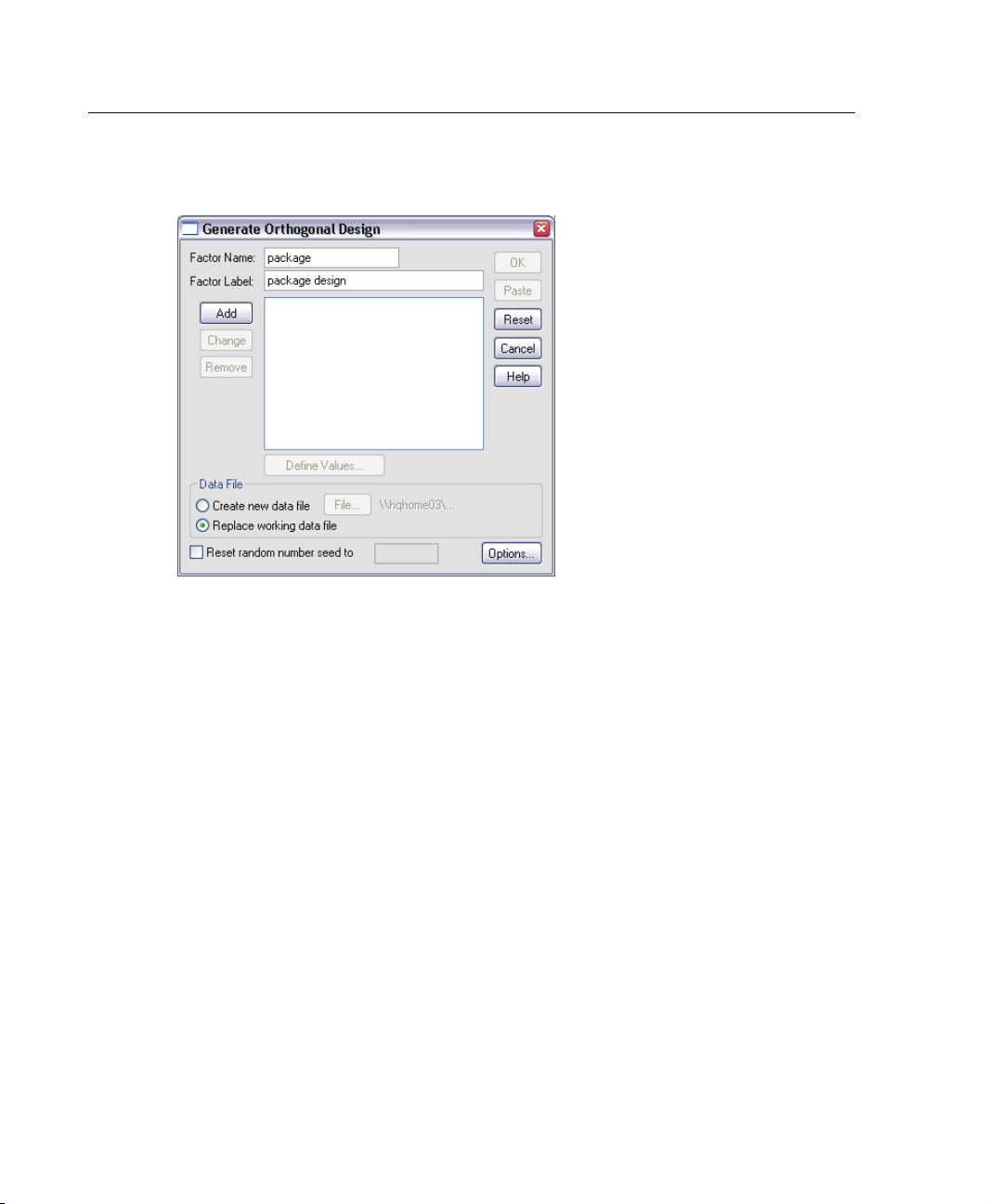
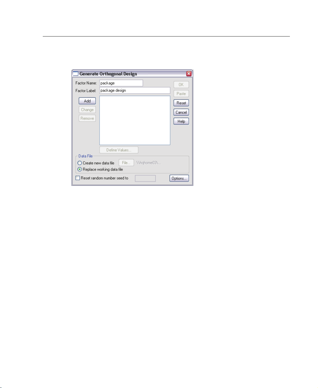
E Define at least one factor. Enter a name in the Factor Name text box. Factor names

can be any valid SPSS variable name, except status_ or card_. Youcanalsoassign
an option

al factor label.

d

E Click Ad

to add the factor name and an optional label. To delete a factor, select it in
the list and click Remove. To modify a factor name or label, select it in the list, modify
the name or label, and click Change.

E Define values for each factor by selecting the factor and clicking Define Values.

Data File. Allows you to control the destination of the orthogonal design. You can

either c

reate a new dataset containing the orthogonal design, or you can replace the

active dataset.

 Create new data file. Creates a new data file containing the factors and cases

generat
to the current directory. Click

ed by the plan. By default, this data file is named ortho.sav,anditissaved

File to specify a different name and destination for

the file.

Replace workin g data file. Replaces the active dataset with the generated plan.



 Reset random number seed to. Resets the random number seed to the specified

value. The seed can be any integer value from 0 through 2,000,000,000. Within
a session, SPSS uses a different seed each time you generate a set of random
numbers, producing different results. If you want to duplicate the same random
numbers, you should set the seed value before you generate your first design and
reset the seed to the same value each subsequent time you generate the design.

Optionally, you can:

 Click Options to specify the minimum number of cases in the orthogonal design

and to select holdout cases.

Defining Values for an Orthogonal Design

Figure 2-2

Generate Design Define Values dialog box

7

Generating an Orthogonal Design

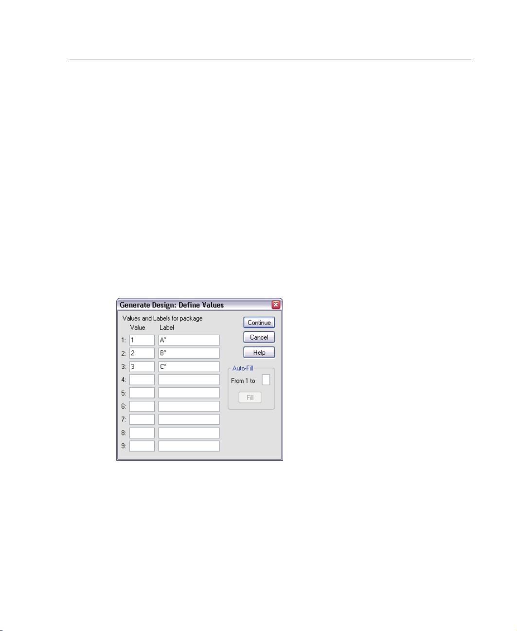
You must assign values to each level o f the selected factor or factors. If you have
selected one factor, the factor name will be displayed after Values and Labels for. If you
have selected multiple factors, the text displays

Values and Labels for Selected Variables.

Enter each value of the factor. You can elect to give the values descriptive labels.
If you do not assign labels to the values, labels that correspond to the values are
automatically assigned (that is, a value of 1 is assigned a label of 1, a value of 3 is
assigned a label of 3, and so on).

8

Chapter 2

Auto-Fill. Allows you to automatically fill the Value boxes with consecutive values

beginning with 1. Enter the maximum value and click Fill to fill in the values.

Orthogonal Design Options

Figure 2-3

Generate Orthogonal Design Options dialog box

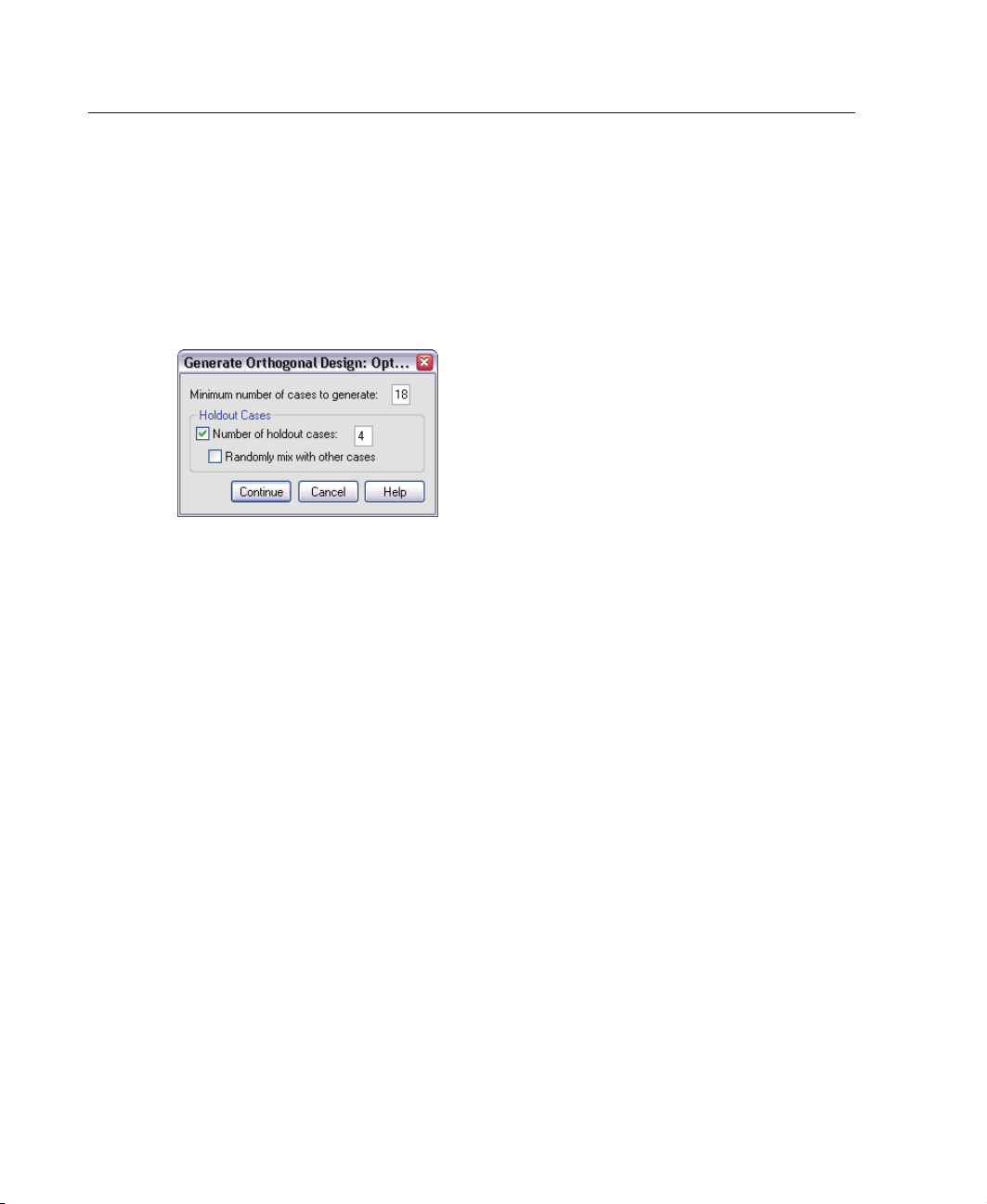
Minimum number of cases to generate. Specifiesaminimumnumberofcasesforthe

plan. Select a positive integer less than or equal to the total number of cases that can be
formed from all possible combinations of the factor levels. If you do not explicitly
specify the minimum number of cases to generate, the minimum number of cases
necessary for the orthogonal plan is generated. If the Orthoplan procedure cannot
generate at least the number of profiles requested for the minimum, it will generate the
largest number it can that fits the specified factors and levels. Note that the design does
not necessarily include exactly the number of specified cases but rather the smallest
possible number of cases in the orthogonal design using this value as a minimum.

Holdout Cases. You can define holdout cases that are rated by subjects but are not

included in the conjoint analysis.

 Number of holdout cases. Creates holdout cases in addition to the regular plan

cases. Holdout cases are judged by the subjects but are not used when the
Conjoint procedure estimates utilities. You can specify any positive integer less
than or equal to the total number of cases that can be formed from all possible
combinations of factor levels. Holdout cases are generated from another random
plan, not the main-effects experimental plan. The holdout cases do not duplicate
the experimental profiles or each other. By default, no holdout cases are produced.

 Randomly mix with other cases. Randomly mixes holdout cases with the

experimental cases. When this option is deselected, holdout cases appear
separately, following the experimental cases.

ORTHOPLAN Command Additional Features

The SPSS command language also allows you to:

 Append the orthogonal design to the active dataset rather than creating a new one.

 Specify simulation cases before generating the orthogonal design rather than after

the design has been created.

See the SPSS Command Syntax Reference for complete syntax information.

9

Generating an Orthogonal Design

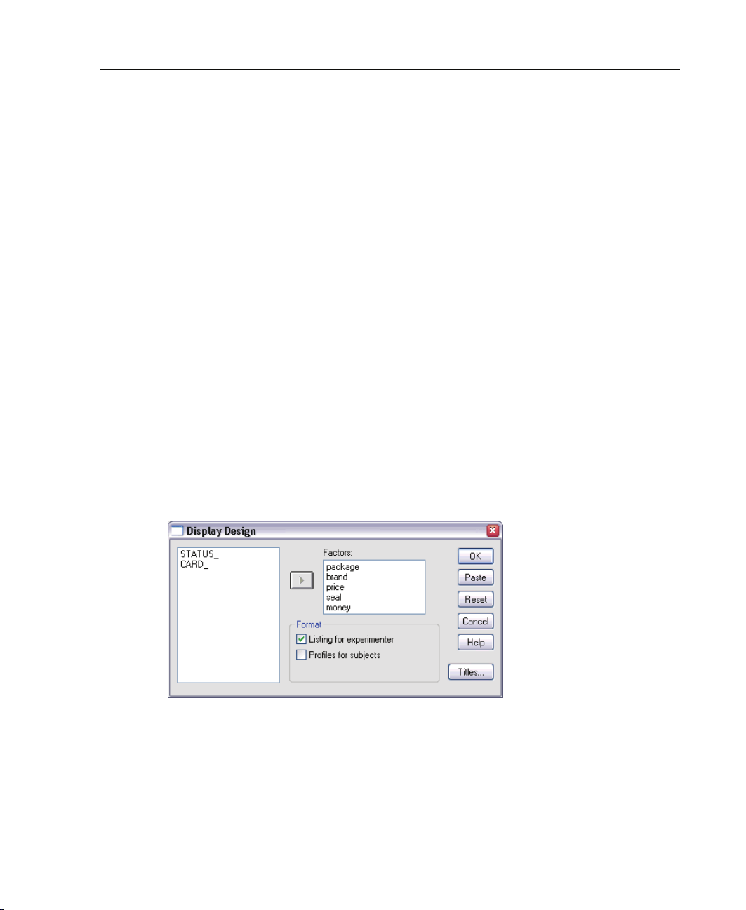
Displaying a Design

The Display Design procedure allows you to print an experimental design. You can
print the design in either a rough-draft listing format or as profiles that you can present
to subjects in a conjoint study. This procedure can display designs created with the
Generate Orthogonal Design procedure or any designs displayed in an active dataset.

To Display an Orthogonal Design

E From the menus choose:

Data

Orthogonal Design

Display...

Figure 3-1

Display Design dialog box

Chapter

3

E Move one or more factors into the Factors list.

E Select a format for displaying the profiles in the output.

11

12

Chapter 3

Format. You can choose one or more of the following format options:

 Listing for experimenter. Displays the design in a draft f ormatthatdifferentiates

holdout profiles from experimental profilesandlistssimulationprofilesseparately
following the experimental and holdout profiles.

 Profiles for subjects. Produces profiles that can be presented to subjects. This format

does not differentiate holdout profiles and does not produce simulation profiles.

Optionally, you can:

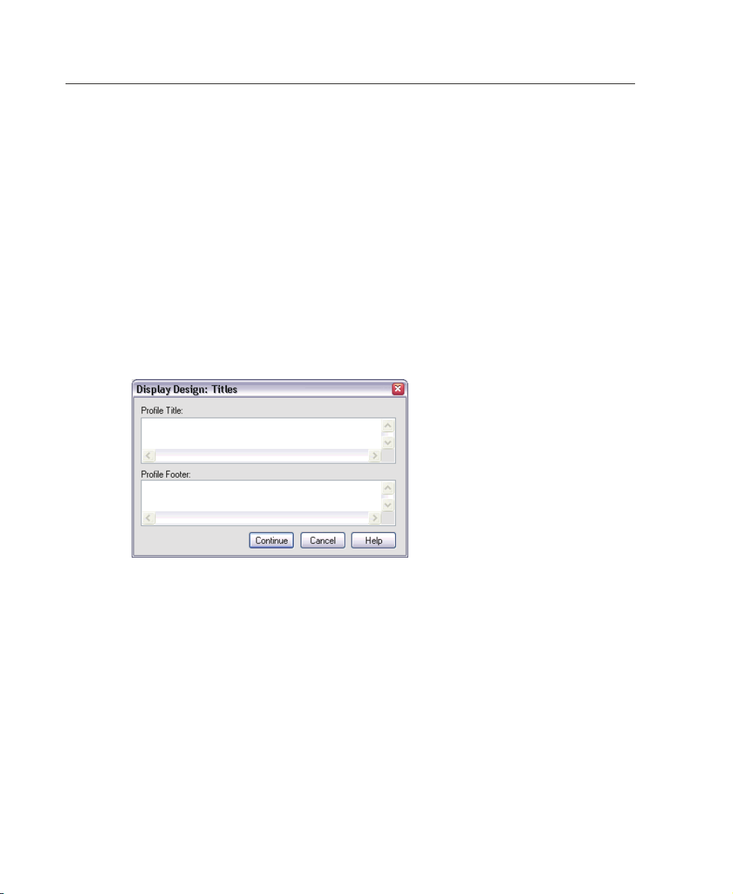
 Click Titles to define headers and footers for the profiles.

Display Design Titles

Figure 3-2

Display Design Titles dialog box

Profile Title. Enter a profile title up to 80 characters long. Titles appear at the top

of the output if you have selected Listing for experimenter andatthetopofeachnew
profile if you have selected

subjects

, if the special character sequence )CARD is specified anywhere in the title, the

Profiles for subjects in the main dialog box. For Profiles for

procedure will replace it with the sequential profile number. This character sequence is
not translated for

Profile F ooter. Enter a profile footer up to 80 characters long. Footers appear at the

bottom of the output if you have select

Listing for experimenter.

ed

Listing for experimenter and at the bottom of

each profile if you have selected Pro f iles for subjects in the main dialog box. For Profiles

for subjects

footer, the procedure will replace
sequence is not translated for

, if the special character sequence )CARD is specified anywhere in the

it with the sequential profile number. This character

Listing for experimenter.

PLANCARDS Command Additional Features

The SPSS command language also allows you to:

 Write profiles for subjects to an external file (using the OUTFILE subcommand).

See the SPSS Command Syntax Reference for complete syntax information.

13

Displaying a Design

Running a Conjoint Analysis

In this release of SPSS, a graphical user interface is not yet available for the Conjoint
procedure. To obtain a conjoint analysis, you must enter command syntax for a

CONJOINT command into a syntax window, and then run it.

 For an example of command syntax for a CONJOINT command in the context of a

complete conjoint analysis—including generating and displaying an orthogonal
design—see “Using Conjoint A nalysis to Model Carpet-Cleaner Preference”.

 For complete command syntax information about the CONJOINT command, see

the SPSS Command Syntax Reference.

To Run a Command from a Syntax Window

Chapter

4

From the menus choose:

File

New

SPSS Syntax...

This opens an SPSS syntax window.

E Enter the command syntax for the CONJOINT command.

E Highlight the command in the syntax window, and click the Run button (the

right-pointing triangle) on the Syntax Editor toolbar.

See the SPSS Base User’s Guide for more information about running commands in
syntax windows.

Requirements

The Conjoint procedure requires two files—a data file and a plan file—and the
specification of how data were recorded (for example, each data point is a preference
score from 1 to 100). The plan file consists of the set of product profiles to be rated

15

16

Chapter 4

by the subjects and should be generated using the Generate Orthogonal Design
procedure. The data file c ontains the preference scores or rankings of those profiles
collected from the subjects. The plan and data files are specified with the PLAN and

DATA subcommands, respectively. The method of data recording is specified with the
SEQUENCE, RANK,orSCORE subcommands. The following command syntax shows a

minimal specification:

CONJOINT PLAN='CPLAN.SAV' /DATA='RUGRANKS.SAV'

/SEQUENCE=PREF1 TO PREF22.

Specifying the Plan File and the Data File

The CONJOINT command provides a number of options for specifying the plan file and
the data file.

 You can explicitly specify the filenames for the two files. For example:

CONJOINT PLAN='CPLAN.SAV' /DATA='RUGRANKS.SAV'

 Ifonlyaplanfileordatafileisspecified,theCONJOINT command reads the

specified file and uses the active dataset as the other. For example, if you specify a
data file but omit a plan file (you cannot omit both), the active dataset is used as
theplan,asshowninthefollowingexample:

CONJOINT DATA='RUGRANKS.SAV'

 You can use the asterisk (*) in place of a filename to indicate the active dataset, as

shown in the following example:

CONJOINT PLAN='CPLAN.SAV' /DATA=*

The active dataset is used as the preference data. Note that you cannot use the
asterisk (*) for both the plan file and the data file.

Specifying How Data Were Recorded

You must specify the way in which preference data were recorded. Data can be
recorded in one of three ways: sequentially, as rankings, or as preference scores. These
three methods are indicated by the SEQUENCE, RANK,andSCORE subcommands.
You must specify one, and only one, of these subcommands as part of a
command.

CONJOINT

17

Running a Conjoint Analysis

SEQUENCE Subcommand

The SEQUENCE subcommand indicates that data were recorded sequentially so that
each data point in the data file is a profile number, starting with the most preferred
profile and ending with the least preferred profile. This is how data are recorded if the
subject is asked to order the profiles from the most to the least preferred. The researcher
records which profile number was first, which profile number was second, and so on.

CONJOINT PLAN=* /DATA='RUGRANKS.SAV'

/SEQUENCE=PREF1 TO PREF22.

The variable PREF1 contains the profile number for the most preferred profile out



of 22 profiles in the orthogonal plan. The variable PREF22 contains the profile
number for the least preferred profile in the plan.

RANK Subcommand

The RANK subcommand indicates that each data point is a ranking, starting with the
ranking of profile 1, then the ranking of profile 2, and so on. This is how the data are
recorded if the subject is asked to assign a rank to each profile, ranging from 1 to n,
where n is the number of profiles. A lower rank implies greater preference.

CONJOINT PLAN=* /DATA='RUGRANKS.SAV'

/RANK=RANK1 TO RANK22.

The variable RANK1 contains the ranking of profile 1, out of a total of 22 profiles



in the orthogonal plan. The variable RANK22 contains the ranking of profile 22.

SCORE Subcommand

The SCORE subcommand indicates that each data point is a preference score assigned
to the profiles, starting with the score of profile 1, then the score of profile 2, and so
on. This type of dat

a might be generated, for example, by asking subjects to assign
a number from 1 to 100 to show how much they liked the profile. A higher score
implies greater preference.

CONJOINT PLAN=* /DATA='RUGRANKS.SAV'

/SCORE=SCORE1 TO SCORE22.

The variable SCORE1 contains the score for profile 1, and SCORE22 contains



the score for profile 22.

18

Chapter 4

Optional Subcommands

The CONJOINT command offers a number of optional subcommands that provide
additional control and functionality beyond what is required.

SUBJECT Subcommand

The SUBJECT subcommand allows you to specify a variable from the data file to
be used as an identifier for the subjects. If you do not specify a subject variable,
the

CONJOINT commandassumesthatallofthecasesinthedatafilecomefrom

one subject. The following example specifies that the variable ID,fromthefile
rugranks.sav, is to be used as a subject identifier.

CONJOINT PLAN=* /DATA='RUGRANKS.SAV'

/SCORE=SCORE1 TO SCORE22 /SUBJECT=ID.

FACTORS Subcommand

The FACTORS subcommand allows you to specify the model describing the expected
relationship between factors and the rankings or scores. If you do not specify a model
for a factor,

DISCRETE. The DISCRETE model indicates that the factor levels are categorical and

CONJOINT assumes a discrete model. You can specify one of four models:

that no assumption is made about the relationship between the factor and the scores or
ranks. This is the default.

LINEAR. The LINEAR model indicates an expected linear relationship between the

factor and the scores or ranks. You can specify the expected direction of the linear
relationship with the keywords MORE and LESS. MORE indicates that higher levels of a
factor are expected to be preferred, while

LESS indicates that lower levels of a factor

are expected to be preferred. Specifying MORE or LESS will not affect estimates of
utilities. They are used simply to identify subjects whose estimates do not match
the expected direction.

IDEAL. The IDEAL model indicates an expected quadratic relationship between the

scores or ranks and the factor. It is assumed that there is an ideal level for the factor,
and distance from this ideal point (in either direction) is associated with decreasing
preference. Factors described with this model should have at least three levels.

19

Running a Conjoint Analysis

ANTIIDEAL. The ANTIIDEAL model indicates an expected quadratic relationship

between the scores or ranks and the factor. It is assumed that there is a worst level for
the factor, and distance from this point (in either direction) is associated with increasing
preference. Factors described with this model should have at least three levels.

The following command syntax provides an example using the

CONJOINT PLAN=* /DATA='RUGRANKS.SAV'

/RANK=RANK1 TO RANK22 /SUBJECT=ID
/FACTORS=PACKAGE BRAND (DISCRETE) PRICE (LINEAR LESS)

Note that both package and brand are modeled as discrete.



SEAL (LINEAR MORE) MONEY (LINEAR MORE).

FACTORS subcommand:

PRINT Subcommand

The PRINT subcommand allows you to control the content of the tabular output. For
example, if you have a large number of subjects, you can choose to limit the output
to summary results only, omitting detailed output for each subject, as shown in the
following example:

CONJOINT PLAN=* /DATA='RUGRANKS.SAV'

/RANK=RANK1 TO RANK22 /SUBJECT=ID
/PRINT=SUMMARYONLY.

You can also choose whether the output includes analysis of the experimental data,
results for any simulation cases included in the plan file, both, or none. Simulation
cases are not rated by the subjects but represent product profiles of interest to you. The
Conjoint procedure uses the analysis of the experimental data to make predictions
about the relative preference for each of the simulation profiles. In the following
example, detailed output for each subject is suppressed, and the output is limited to
results of the simulations:

CONJOINT PLAN=* /DATA='RUGRANKS.SAV'

/RANK=RANK1 TO RANK22 /SUBJECT=ID
/PRINT=SIMULATION SUMMARYONLY.

20

Chapter 4

PLOT Subcommand

The PLOT subcommand controls whether plots are included in the output. Like
tabular output (PRINT subcommand), you can control whether the output is limited to
summary results or includes results for each subject. By default, no plots are produced.
In the following example, output includes all available plots:

CONJOINT PLAN=* /DATA='RUGRANKS.SAV'

/RANK=RANK1 TO RANK22 /SUBJECT=ID
/PLOT=ALL.

UTILITY Subcommand

The UTILITY subcommand writes an SPSS data file containing detailed information
for each subject. It includes the utilities for DISCRETE factors, the slope and quadratic
functions for

LINEAR, IDEAL,andANTIIDEAL factors, the regression constant, and

the estimated preference scores. These values can then be used in further analyses or
for making additional plots with other procedures. The following example creates
a utility file named rugutil.sav:

CONJOINT PLAN=* /DATA='RUGRANKS.SAV'

/RANK=RANK1 TO RANK22 /SUBJECT=ID
/UTILITY='RUGUTIL.SAV'.

Chapter

Using Conjoint Analysis to Model Carpet-Cleaner Preference

In a popular example of conjoint analysis (Green and Wind, 1973), a company
interested in marketing a new carpet cleaner wants to examine the influence of
five factors on consumer preference—package design, brand name, price, a Good
Housekeeping seal, and a money-back guarantee. There are three factor levels for
package design, each one differing in the location of the applicator brush; three brand
names (K2R, Glory,andBissell); three price levels; and two levels (either no or yes)
for each of the last two factors. The following table displays the variables used in the
carpet-cleaner study, with their variable labels and values.

Tab l e 5 -1

Variables in the carpet-cleaner study

5

Variable name Variable label Value label

package

brand

price

seal
money

There could be other factors and factor levels that characterize carpet cleaners, but these
are the only ones of interest to management. This is an important point in conjoint
analysis. You want to choose only those factors (independent variables) that you think
most influence the subject’s preference (the dependent variable). Using conjoint
analysis, you will develop a model for customer preference based on these five factors.

This example makes use of the information in the following data files:

carpet_prefs.sav contains the d ata collected from the subjects; carpet_plan.sav
contains the product profiles being surveyed; conjoint.sps contains the command

package design A*, B*, C*

brand name K2R, Glory, Bissell

price

Good Housekeeping seal

money-back guarantee

21

$1.19, $1.39, $1.59
no, yes

no, yes

22

Chapter 5

syntax necessary to run the analysis. The files are located in the tutorial\sample_files
folder of the SPSS installation folder.

Generating an Orthogonal Design

The first step in a conjoint analysis is to create the combinations of factor levels that are
presented as product profiles to the subjects. Since even a small number of factors and
a few levels for each factor will lead to an unmanageable number of potential product
profiles, you need to generate a representative subset known as an orthogonal array.

The Generate Orthogonal Design procedure creates an orthogonal array—also
referred to as an orthogonal design—and stores the information in an SPSS data
file. Unlike most SPSS procedures, an active dataset is not required before running
the Generate Orthogonal Design procedure. If you do not have an active dataset,
you have the option of creating one, generating variable names, variable labels, and
value labels from the options that you select in the dialog boxes. If you already have
an active dataset, you can either replace it or save the orthogonal design a s a separate
SPSS data file.

To create an orthogonal design:

E From the menus choose:

Data

Orthogonal Design

Generate...

Using Conjoint Analysis to Model Carpet-Cleaner Preference

Figure 5-1

Generate Orthogonal Design dialog box

E Enter package in the Factor Name text box, and enter package design in the Factor

Labeltextbox.

23

E Click Add.

This create

E Click Defi

s an item labeled package ‘package design’ (?). Select this item.

ne Values

.

24

Chapter 5

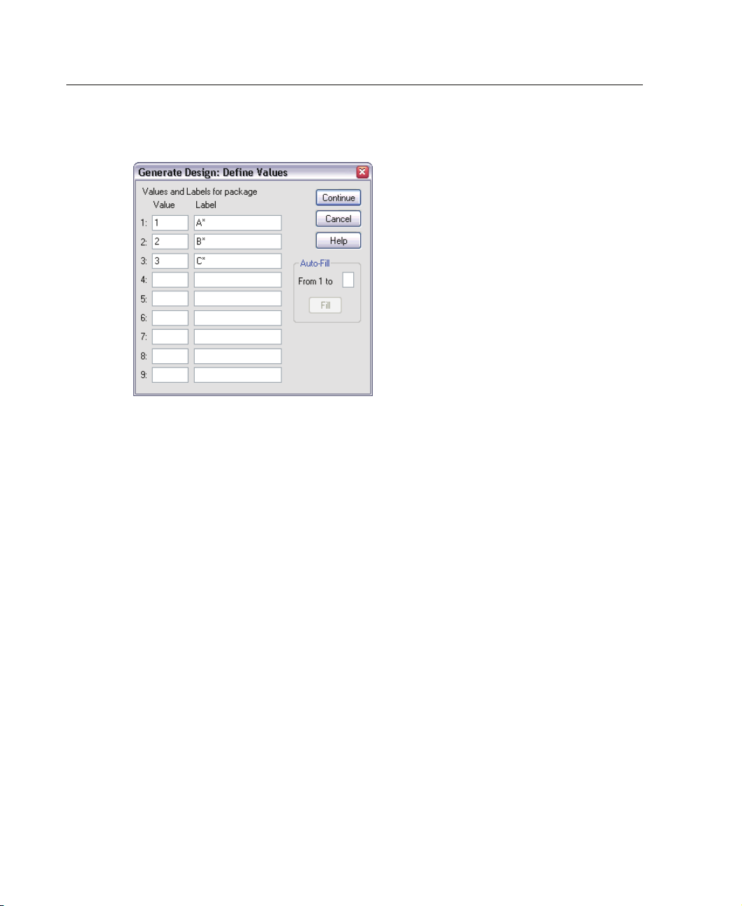
Figure 5-2

Generate Design Define Values dialog box

E Enter the values 1, 2,and3 to represent the package designs A*, B*,andC*.Enterthe

labels A*, B*,andC* as well.

E Click Continue.

You’ll now want to repeat this process for the remaining factors, brand, price, seal,
and money. Use the values and labels from the following table, which includes the
values you’ve already entered for package.

Factor Values Labels

package 1,2,3 A*,B*,C*

brand 1, 2, 3 K2R, Glory, Bissell

price

seal 1, 2
money

1.19, 1.39, 1.59

1, 2

$1.19, $1.39, $1.59
no, yes

no, yes

Once you have completed the factor specifications:

E Select Replace working data file in the Data File group in the Generate Orthogonal

Design dialog box. The generated design will replace the active dataset.

Using Conjoint Analysis to Model Carpet-Cleaner Preference

Select Reset random number seed to and enter the value 2000000.

E

Generating an orthogonal design requires a set of random numbers. If you want to
duplicate a design—in this case, the design used for the present case study—you need
to set the seed value before you generate the design and reset it to the same value each
subsequent time you generate the design. The design used for this case study was
generated with a seed value of 2000000.

E Click Options.

Figure 5-3

Generate Orthogonal Design Options dialog box

25

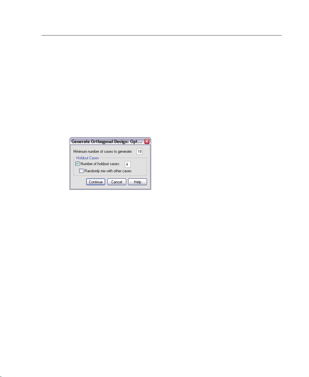
E In the Minimum Number of Cases to Generate text box, type 18.

By default, the minimum number of cases necessary for an orthogonal array is
generated. The procedure determines the number of cases that need to be administered
to allow estimation of the utilities. You can also specify a minimum n

umber of cases to
generate, as you’ve done here. You might want to do this because the default number
of minimum cases is too small to be useful or because you have experimental design
considerations that require a certain minimum number o f cases.

E Select Number of holdout cases and type 4.

Holdout cases are judged by the subjects but are not used by the conjoint analysis to
estimate utilities. They are used as a check on the validity of the estimated utilities.
The holdout cases are generated from another random plan, not the experimental
orthogonal plan.

E Click Continue in the Generate Orthogonal Design Options dialog box.

E Click OK in the Generate Orthogonal Design dialog box.

26

Chapter 5

Figure 5-4

Orthogonal design for the carpet-cleaner example

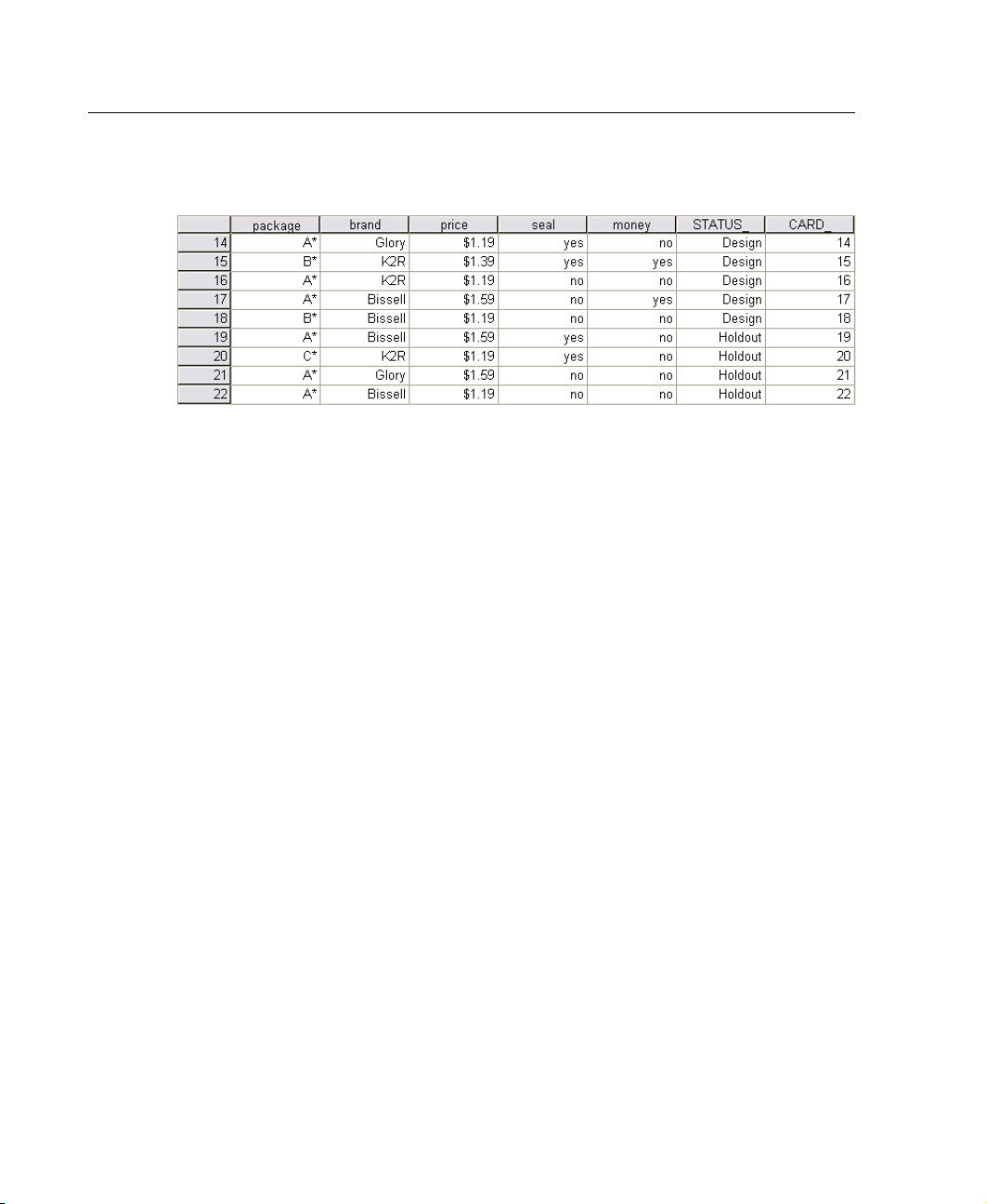
The orthogonal design is displayed in the Data Editor and is best viewed by displaying
value labels rather than the actual data values. This is accomplished by choosing

Value Labels from the View menu.

The variables in the data file are the factors used to specify the design. Each case

represents one product profile in the design. Notice that two additional variables,
CARD_ and STATUS_, appear in the data file. CARD_ assigns a sequential number to
each profile that is used to identify the profile. STATUS_ indicates whether a profile is
part of the experimental design (the first 18 cases), a holdout case (the last 4 cases), or
a simulation case (to be discussed in a later t opic in this case study).

The orthogonal design is a required input to the analysis of the data. Therefore, you

will want to save your design as an SPSS data file. For convenience, the current design
has been saved in carpet_plan.sav (orthogonal designs are also referred to as plans).

Creating the Experimental Stimuli: Displaying the Design

Once you have created an orthogonal design, you’ll want to u se it to create the product
profiles to be rated by the subjects. You can obtain a listing of the profiles in a single
table or display each profile in a separate table.

To display an orthogonal design:

E From the menus choose:

Data

Orthogonal Design

Display...

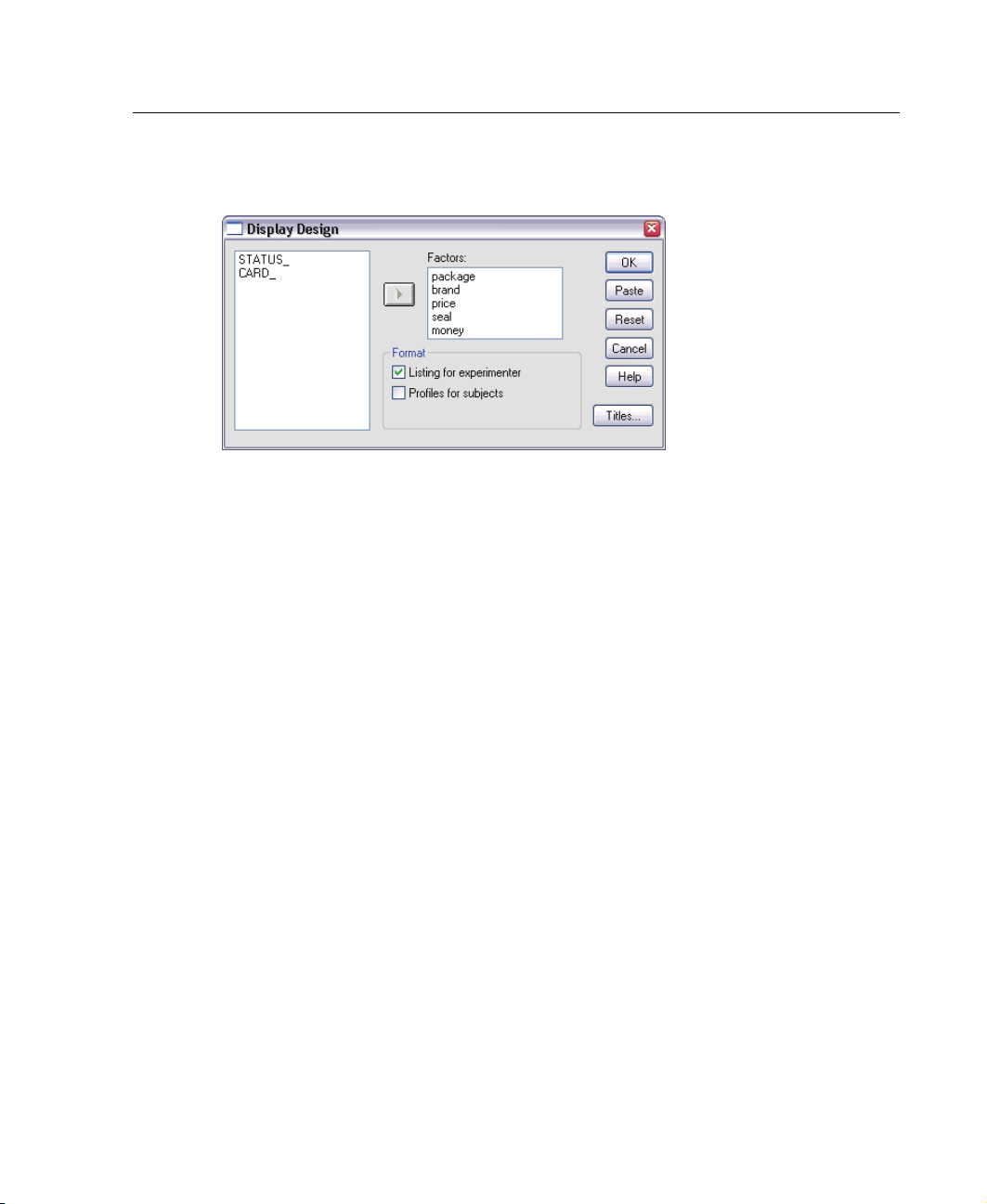
Figure 5-5

Display Design dialog box

27

Using Conjoint Analysis to Model Carpet-Cleaner Preference

E Select pack

age, brand, price, seal,andmoney for the factors.

The information contained in t he variables STATUS_ and CARD_ is automatically
included in the output, so they don’t need to be selected.

E Select Listing for experimenter in the Format group. This results in displaying the entire

orthogonal d

E Click OK.

esigninasingletable.

28

Chapter 5

Figure 5-6

Display of orthogonal design: Single table layout

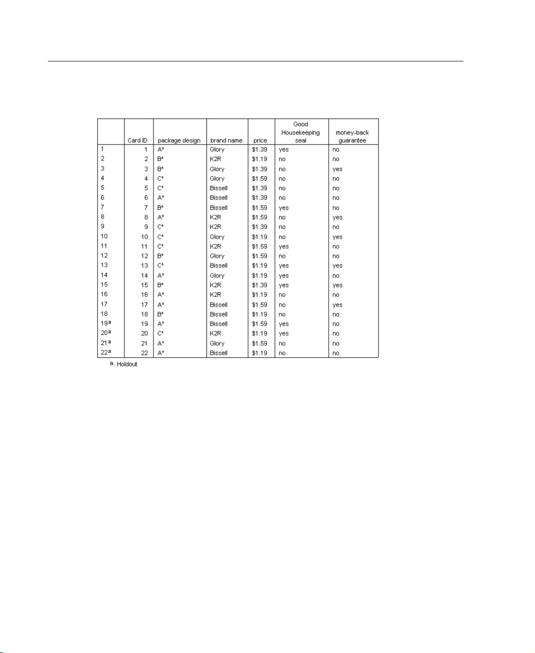
The output resembles the look of the orthogonal design as shown in the Data
Editor—one row for each profile, with the factors as columns. Notice, however, that
the column headers are the variable labels rather than the variable names that you see
in the Data Editor. Also notice that the holdout cases are identified with a footnote.
This is of interest to the experimenter, but you certainly don’t want the subjects to
know which, if any, cases are holdouts.

Depending on how you create and deliver your final product profiles, you may want
to save this table as an HTML, Word/RTF, Excel, or PowerPoint file. This is easily
accomplished by selecting the table in the Viewer, right clicking, and selecting

Export.

Also, if you’re using the exported version to create the final product profiles, be sure to
edit out the footnotes for the h oldout cases.

Perhaps the needs for your survey are better served by generating a separate table
for each product profile. This choice lends itself nicely to exporting to PowerPoint,
since each table (product profile) is placed on a separate PowerPoint slide.

Using Conjoint Analysis to Model Carpet-Cleaner Preference

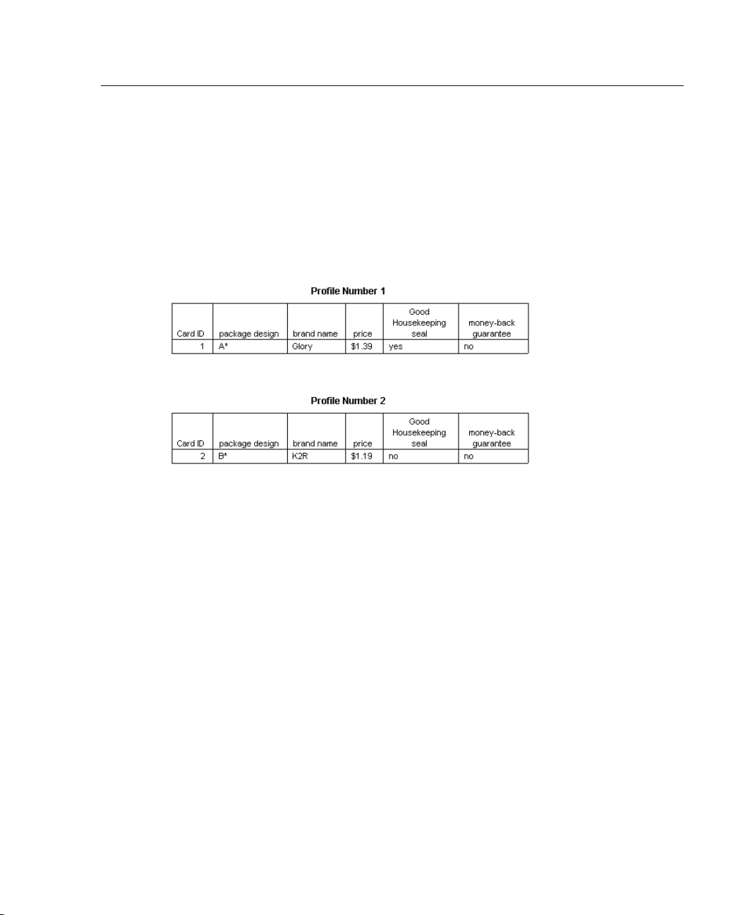
To display each profile in a separate table:

E Click the Dialog Recall button and select Display Design.

E Deselect Listing for experimenter and select Profiles for subjects.

E Click OK.

Figure 5-7

Display of orthogonal design: Multitable layout

29

The informat

ion for each product profile is displayed in a separate table. In addition,
holdout cases are indistinguishable from the rest of the cases, so there is no issue of
removing identifiers for holdouts as with the single table layout.

Running the Analysis

You’ve generated an orthogonal design and learned how to display the associated
product profiles. You’re now ready to learn how to run a conjoint analysis.

30

Chapter 5

Figure 5-8

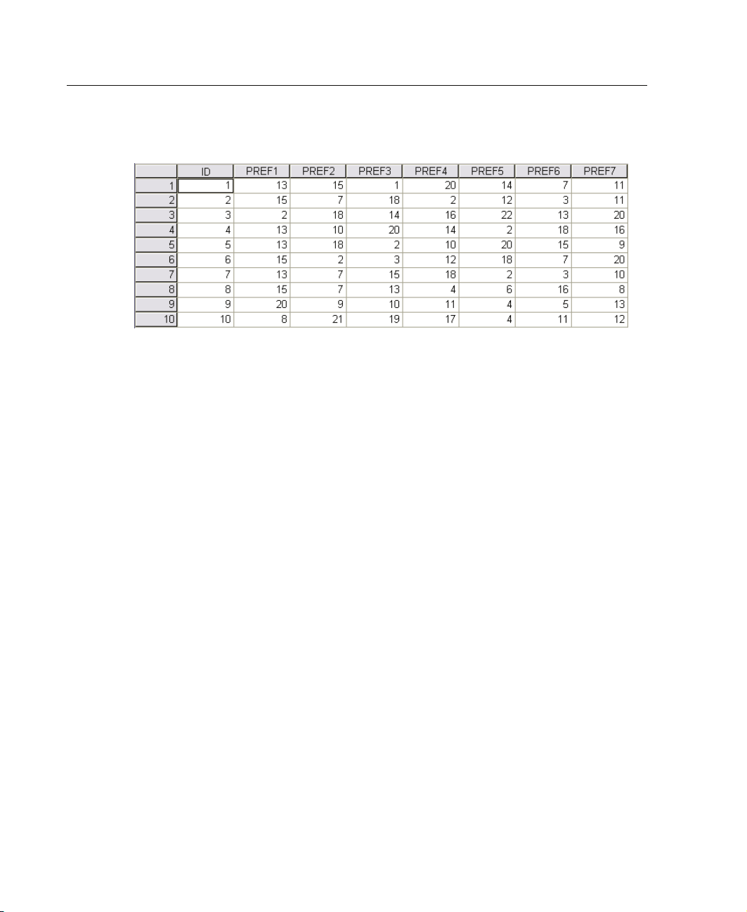
Preference data for the carpet-cleaner example

The preference data collected from the subjects is stored in carpet_prefs.sav.Thedata
consist of responses from 10 subjects, each identified by a unique value of the variable
ID. Subjects were asked to rank the 22 product profiles from the most to the least
preferred. The variables PREF1 through PREF22 contain the IDs of the associated
product profiles, that is, the card IDs from carpet_plan.sav. Subject 1, for example,
liked profile 13 most of all, so PREF1 has the value 13.

Analysis of the data is a task that requires the use of command syntax—specifically,

the

CONJOINT command. The necessary command syntax has been provided in the

file conjoint.sps.

CONJOINT PLAN='file specification'

/DATA='file specification'
/SEQUENCE=PREF1 TO PREF22
/SUBJECT=ID
/FACTORS=PACKAGE BRAND (DISCRETE)

PRICE (LINEAR LESS)
SEAL (LINEAR MORE) MONEY (LINEAR MORE)

/PRINT=SUMMARYONLY.

The PLAN subcommand specifies the file containing the orthogonal design—in



this example, carpet_plan.sav.

 The DATA subcommand specifies the file containing the preference data—in this

example, carpet_prefs.sav. If you choose the preference data as the active dataset,
you can replace the file specification with an asterisk (*), without the quotation
marks.

 The SEQUENCE subcommand specifies that each data point in the preference data

is a profile number, starting with the most-preferred profile andendingwiththe
least-preferred profile.

31

Using Conjoint Analysis to Model Carpet-Cleaner Preference

The SUBJECT subcommand specifies that the variable ID identifies the subjects.



 The FACTORS subcommand specifies a model describing the expected relationship

between the preference data and the factor levels. The specified factors refer to
variables defined in the plan file named on the

 The keyword DISCRETE is used when the factor levels are categorical and no

PLAN subcommand.

assumption is made about the relationship between the levels and the data. This
is the case for the factors package and brand that represent package design and
brand name, respectively.
of the four alternatives (
included on the

 The keyword LINEAR, used for the remaining factors, indicates that the data are

FACTORS subcommand.

DISCRETE is assumed if a factor is not labeled with one

DISCRETE, LINEAR, IDEAL, ANTIIDEAL), or is not

expected to be linearly related to the factor. For example, preference is usually
expected to be linearly related to price. You can also specify quadratic models (not
used in this example) with the keywords

 The keywords MORE and LE SS, following LINEAR, indicate an expected direction

IDEAL and ANTIIDEAL.

for the relationship. Since we expect higher preference for lower prices, the
keyword

LESS is used for price. However, we expect higher preference for either a

Good Housekeeping seal of approval or a money-back guarantee, so the keyword

MORE is used for seal and money (recall that the levels for both of these factors

weresetto1forno and2foryes).

Specifying

MORE or LESS does not change the signs of the coefficients or affect

estimates of the utilities. These keywords are used simply to identify subjects
whose estimates do not match the expected direction. Similarly, choosing

IDEAL

instead of ANTIIDEAL, or vice versa, does not affect coefficients or utilities.

 The PRINT subcommand specifies that the output contains information for the

group of subjects only as a whole (

SUMMARYONLY keyword). Information for

each subject, separately, is suppressed.

Try running this command syntax. Make sure that you have included valid paths to
carpet_prefs.sav and carpet_plan.sav. For a complete description of all options, see

CONJOINT commandintheSPSS Command Syntax Reference.

the

32

Chapter 5

Utility Scores

Figure 5-9

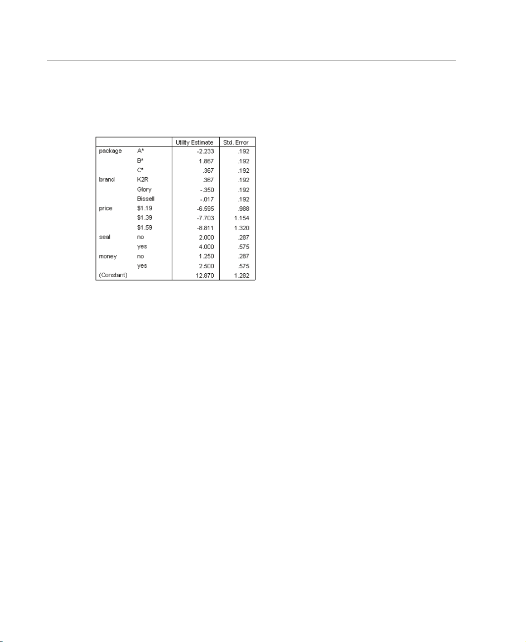
Utility scores

This table shows the utility (part-worth) scores and their standard errors for each factor
level. Hig
relationship between price and utility, with higher prices corresponding to lower utility
(larger negative values mean lower utility). The presence of a seal of approval or
money-bac

Since the utilities are all expressed in a common unit, they can be added together
to give the total utility of any combination. For example, the total utility of a
cleaner w
money-back guarantee is:

her utility values indicate greater preference. As expected, there is an inverse

k guarantee corresponds to a higher utility, as anticipated.

ith package design B*,brandK2R,price$1.19, and no seal of approval or

utility(package B*) + u tility(K2R) + utility($1.19)

+ utility(no seal) + utility(no money-back) + constant

or

1.867 + 0.367 + (–6.595) + 2.000 + 1.250 + 12.870 = 11.759

If the cleaner had package design C*,brandBissell,price$1.59, a seal of approval,
and a money-back guarantee, the total utility would be:

0.367 + (–0.017) + (–8.811) + 4.000 + 2.500 + 12.870 = 10.909

Coefficients

Figure 5-10

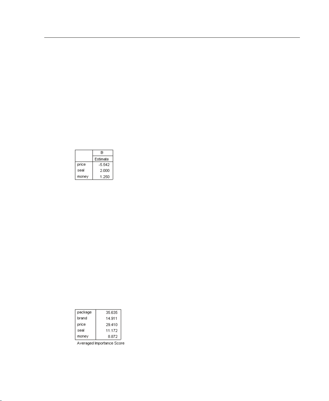
Coefficients

This table shows the linear regression coefficients for those factors specified as

LINEAR (for IDEAL and ANTIIDEAL models, there would also be a quadratic term).

The utility for a particular factor level is determined by multiplying the level by the
coefficient. For example, the predicted utility for a price of $1.19 was listed a s –6.595
in the utilities table. This is simply the value of the price l evel, 1.19, multiplied by the
price coefficient, –5.542.

33

Using Conjoint Analysis to Model Carpet-Cleaner Preference

Relative Importance

The range of the utility values (highest to lowest) for each factor provides a measure of
how important the factor was to overall preference. Factors with greater utility ranges
play a more significant role than those with smaller ranges.

Figure 5-11

Importance values

34

Chapter 5

This table provides a measure of the relative importance of each factor known as an
importance score or value. The values are computed by taking the utility range for
each factor separately and dividing by the sum of the utility ranges for all factors. The
values thus represent percentages and have the property that they sum to 100. The
calculations, it should be noted, are done separately for each subject, and the results
are then averaged over all of the subjects.

Note that while overall or summary utilities and regression coefficients from
orthogonal designs are the same with or without a

SUBJECT subcommand, importances

will generally differ. For summary results without a SUBJECT subcommand, the
importances can be computed directly from the summary utilities, just as one can
do with individual subjects. However, when a

SUBJECT subcommand is used, the

importances for the individual subjects are averaged, and these averaged importances
will not in general match those computed using the summary utilities.

The results show that package design has the most influence on overall preference.
This means that there is a large difference in preference between product profiles
containing the most desired packaging and those containing the least desired packaging.
The results also show that a money-back guarantee plays the least important role in
determining overall preference. Price plays a significant role but not as significant as
package design. Perhaps this is because the range of prices is not that large.

Correlations

Figure 5-12

Correlation coefficients

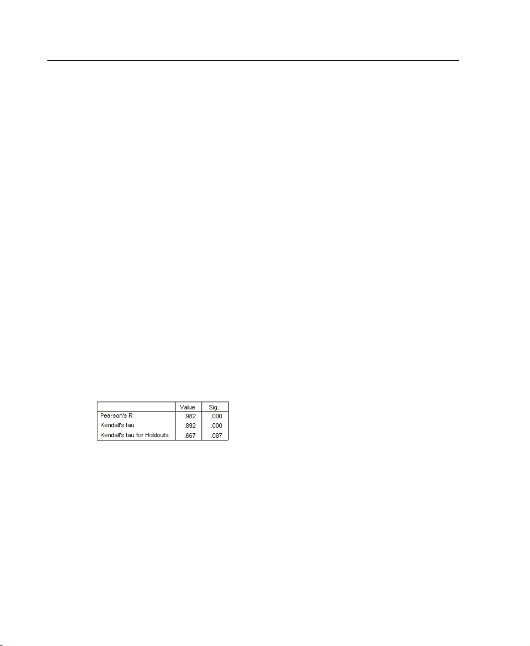
This table displays two statistics, Pearson’s R and Kendall’s tau, which provide
measures of the correlation between the observed and estimated preferences.

The table also displays Kendall’s tau for just the holdout profiles. Remember that
the holdout profiles (4 in the present example) were rated by the subjects but not used
by the Conjoint procedure for estimating utilities. Instead, the Conjoint procedure
computes correlations between the observed and predicted rank orders for these
profiles as a check on the validity of the utilities.

profiles rated, which will artificially inflate the correlation between observed and
estimated scores. In these cases, the correlations for the holdout profiles may give a
better indication of the fit of the model. Keep in mind, however, that holdouts will
always produce lower correlation coefficients.

Reversals

When specifying LINEAR models for price, seal,andmoney, we chose an expected
direction (LESS or MORE) for the linear relationship between the value of the variable
and the preference for that value. The Conjoint procedure keeps track of the number
of subjects whose preference showed the opposite of the expected relationship—for
example, a greater preference for higher prices, or a lower preference for a money-back
guarantee. These cases are referred to as reversals.

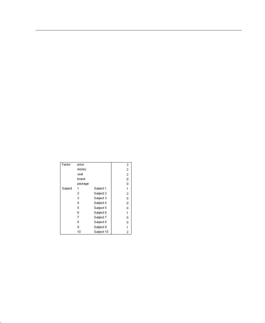
Figure 5-13

Number of reversals by factor and subject

35

Using Conjoint Analysis to Model Carpet-Cleaner Preference

In many conjoint analyses, the number of parameters is close to the number of

This table displays the number of reversals for each factor and for each subject. For
exampl

e, three subjects showed a reversal for price. That is, they preferred product

profiles with higher prices.

36

Chapter 5

Running Simulations

The real power of conjoint analysis is the ability to predict preference for product
profiles that weren’t rated by the subjects. These are referred to as simulation cases.
Simulation cases are included as part of the plan, along with the profiles from the
orthogonal design and any holdout profiles.

The simplest way to enter simulation cases is from the Data Editor, using the value
labels created when you generated the experimental design.

To enter a simulation case in the plan file:

E On a new row in the Data Editor window, select a cell and select the desired value from

the list (value labels can be displayed by choosing Value Labels from the View menu).
Repeat for all of the variables (factors).

E Select Simulation forthevalueoftheSTATUS_ variable.

E Enter an integer value, to be used as an identifier, for the CARD_ variable. Simulation

cases should be numbered separately from the other cases.

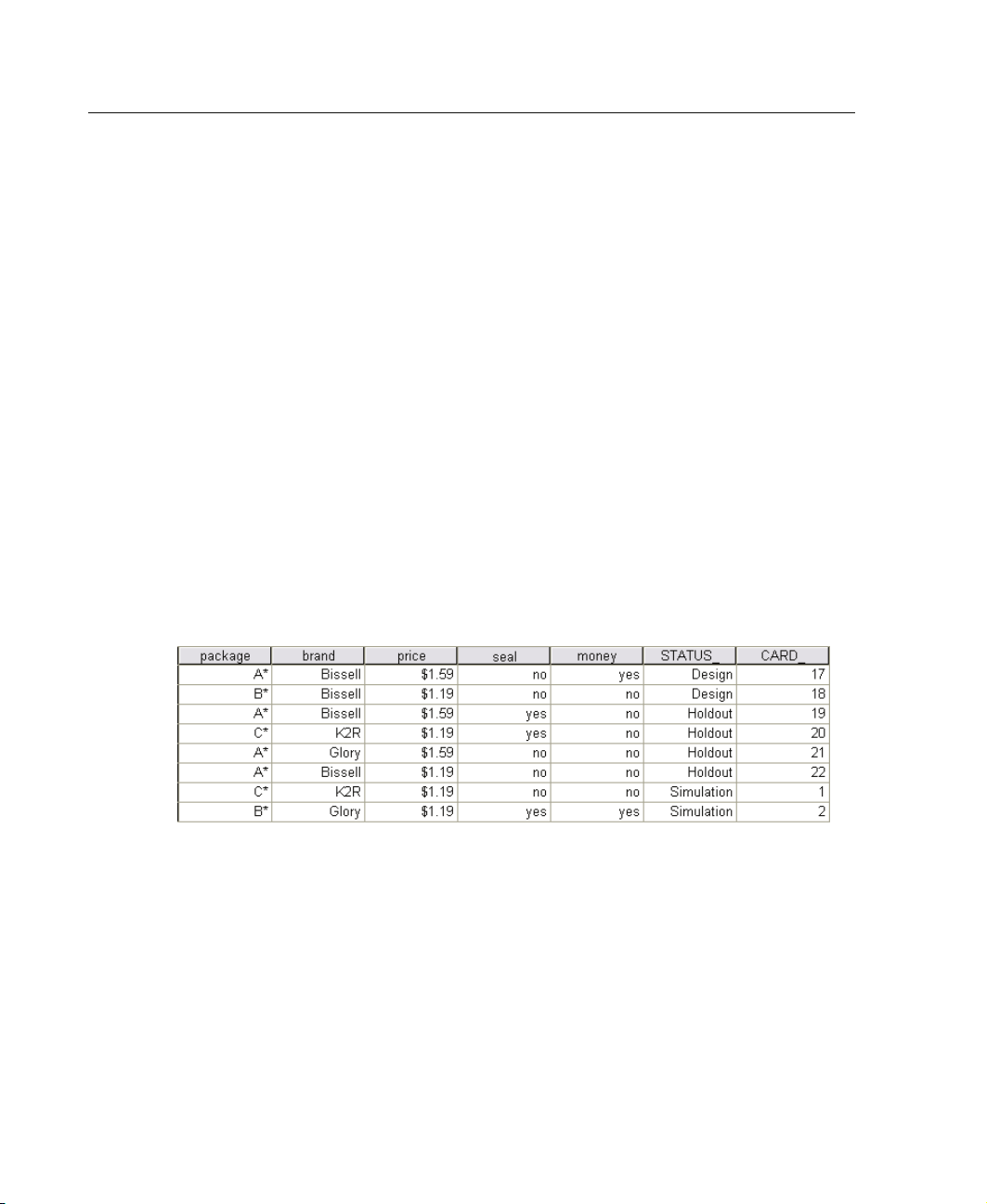
Figure 5-14

Carpet-cleaner data including simulation cases

The figure shows a part of the plan file for the carpet-cleaner study, with two simulation
cases added. For convenience, these have been included in carpet_plan.sav.

The analysis of the simulation cases is accomplished with the same command
syntax used earlier, that is, the syntax in the file conjoint.sps. In fact, if you ran the
syntax described earlier, you would have noticed that the output also includes results
for the simulation cases, since they are included in carpet_plan.sav.

You can choose to run simulations along with your initial analysis—as done
here—or run simulations at any later point simply by including simulation cases in
your plan file and rerunning

CONJOINT. For more information, see the CO NJOINT

command in the SPSS Command Syntax Reference.

Using Conjoint Analysis to Model Carpet-Cleaner Preference

Preference Probabilities of Simulations

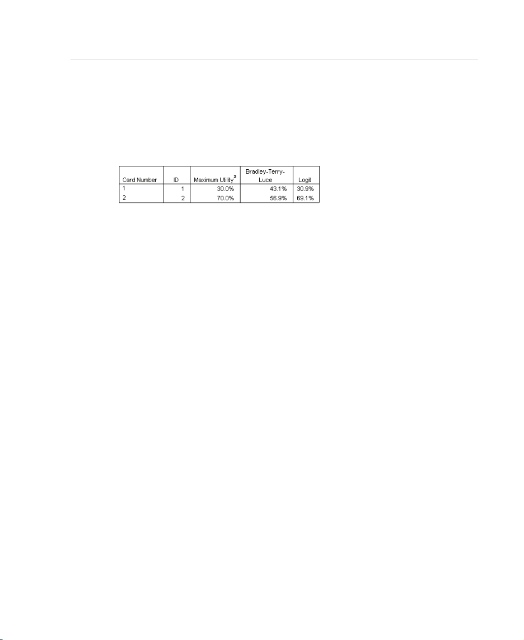
Figure 5-15

Simulation results

This table gives the predicted probabilities of choosing each of the simulation cases
as the most preferred one, under three different probability-of-choice models. The
maximum utility model determines the probability as the number of respondents
predicted to choose the profile divided by the total number of respondents. For each
respondent, the predicted choice is simply the profile with the largest total utility.
The BTL (Bradley-Terry-Luce) model determines the probability as the ratio of a
profile’s utility to that for all simulation profiles, averaged across all respondents.
The logit model is similar to BTL but u ses the natural log of the utilities instead of
the utilities. Across the 10 subjects in this study, all three models indicated that
simulation profile 2 would be preferred.

37

Bibliography

Akaah, I. P., and P. K. Korgaonkar. 1988. A conjoint investigation of the relative
importance of risk relievers in direct marketing. Journal of Advertising Research,
28:4, 38–44.

Cattin, P., and D. R. Wittink. 1982. Commercial use of conjoint analysis: A survey.
Journal of Marketing, 46:3, 44–53.

Green, P. E., and Y. Wind. 1973. Multiattribute decisions in marketing: A measurement
approach. Hinsdale, Ill.: Dryden Press.

39

Index

anti-ideal model, 31

BTL (Bradley-Terry-Luce) model

)CARD

in Display Design

card_ variable

in Generate Orthogonal Design
coefficients
command syntax

CONJOINT command
correlation coefficients

data files

in Generate Orthogonal Design
discrete model
Display Design

)CARD

footers

listing format

saving profiles

single-profile format

titles

, 33

, 12

, 12

, 12

, 12

, 30

, 34

, 31

, 3, 11, 26

, 11

, 13

, 11

, 37

, 5

, 5

Generate Orthogonal Design

data files
defining factor names, labels, and values
holdout cases
minimum cases
random number seed
simulation cases

holdout cases

in Generate Orthogonal Design

ideal model
importance scores
importance values

Kendall’s tau

linear model
listing format

in Display Design

logit model

, 5

, 8

, 8

, 9

, 2

, 31

, 33
, 33

, 34

, 31

, 37

, 3, 5, 22

, 5

, 8

, 11

, 7

factor levels
factors
footers

in Display Design
full-profile approach

, 2, 21–22

, 2, 21–22

, 12

, 2

max utility model

orthogonal array
orthogonal designs

displaying
generating
holdout cases

41

, 37

, 2

, 11, 26

, 5, 22

, 8

42

Index

minimum cases, 8

part-worths
Pearson’s R

random number seed

in Generate Orthogonal Design

reversals

sample size
simulation cases

in Generate Orthogonal Design

simulation results

BTL (Bradley-Terry-Luce) model
logit model
max utility model

single-profile format

in Display Design

status_ variable

in Generate Orthogonal Design

syntax

CONJOINT command

, 4

, 34

, 35

, 3

, 4, 19, 36

, 37

, 37

, 11

, 30

, 5

, 9

, 37

, 5

titles

in Display Design

total utility

utility scores

, 32

, 12

, 4, 32