Spss CLASSIFICATION TREES 13.0 User Manual

SPSS Classification Trees™ 13.0

For more information about SPSS®software products, please visit our Web site at http://www.spss.com or contact

SPSS Inc.
233 South Wacker Drive, 11th Floor
Chicago, IL 60606-6412
Tel: (312) 651
Fax: [phone]

SPSS is a registered trademark and t he other product names are the t rademarks of SPSS Inc. for its proprietary computer
software. No m
the trademark and license rights in the software and the copyrights in the published materials.

The SOFTWARE and documentation are provided with RESTRICTED R IGHTS. Use, duplication , or disclosure by the
Governmentis
clause at 52.227-7013. Contractor/manufacturer is SPSS Inc., 233 South Wacker Drive, 11th Floor, Chicago, IL 60606-6412.

General notice: Other product names mentioned herein are used for identification purposes only and may be trademarks of
their respec

TableLook is a trademark of SPSS Inc.
Windows is a registered trademark of Microsoft Corporation.
DataDirect, D
Portions of this product were created using LEADTOOLS © 1991–2000, LEAD Technologies, Inc. ALL RIGHTS RESERVED.
LEAD, LEADTOOLS, and LEADVIEW are registered trademarks of LEAD Technologies, Inc.
Sax Basic is a t
All rights reserved.
Portions of this product were based on the work of the FreeType Team (http://www.freetype.org).
A portion of th
software is provided “as is,” without express or implied warranty.
A portion of the SPSS software contains Sun Java Runtime libraries. Copyright © 2003 by Sun Microsystems, Inc. All rights
reserved. The
licensed from IBM and are available at http://oss.software.ibm.com/icu4j/.

SPSS Classification Trees™ 13.0
Copyright © 20
All rights reserved.
Printed in the United States of America.

No part of this p
electronic, mechanical, photocopying, recording, or otherwise, without the prior written permission of the publisher.

1234567890 07060504

ISBN 1-56827-

-3000

aterial describing such software may be produced or distributed without the written permission of the owners of

subject to restrictions as set forth in subdivision (c) (1) (ii) of The Rights in Technical Data and Computer Software

tive companies.

ataDirect Connect, INTERSOLV,and SequeLink are registered trademarks of DataDirect Technologies.

rademark of Sax Software Corporation. Copyright © 1993–2004 by Polar Engineering and Consulting.

e SPSS software contains zlib technology. Copyright © 1995–2002 by Jean-loup Gailly and Mark Adler. The zlib

Sun Java Runtime libraries include code licensed from RSA Security, Inc. Some portions of the libraries are

04 by SPSS Inc.

ublication may be reproduced, stored in a retrieval system, or transmitted, in any form or by any means,

354-1

Preface

SPSS 13.0 is a comprehensive system for analyzing data. The Classification Trees
optional a
manual. The Classification Trees add-on module must be used with the SPSS 13.0
Basesystemandiscompletelyintegratedintothatsystem.

Installation

To install the Classification Trees add-on module, run the License Authorization
Wizard using the authorization code that you received from SPSS Inc. For more
informat

Compatibility

SPSS is designed to run on many computer systems. See the installation instructions
that cam
requirements.

dd-on module provides the additional analytic techniques described in this

ion, see the installation instructions supplied with the SPSS Base system.

e with your system for specific information on minimum and recommended

Serial N

Your ser
this serial number when you contact SPSS Inc. for information regarding support,
payment, or an upgraded system. The serial number was provided with your Base
system

Customer Service

If you have any questions concerning your shipment or account, contact your local
office
your serial number ready for identification.

umbers

ial number is your identification number with SPSS Inc. You will need

.

, listed on the SPSS Web site at http://www.spss.com/worldwide. Please have

iii

Training Seminars

SPSS Inc. provides both public and onsite training seminars. All seminars feature
hands-on workshops. Seminars will be offered in major cities on a regular basis. For
more informa

tion on these seminars, contact your local office, listed on the SPSS

Web site at http://www.spss.com/worldwide.

Technical S

The service

upport

s of SPSS Technical Support are available to registered customers.
Customers may contact Technical Support for assistance in using SPSS or for
installation help for one of the supported hardware environments. To reach Technical
Support, s

ee the SPSS Web site at http://www.spss.com, or contact your local office,
listedontheSPSSWebsiteathttp://www.spss.com/worldwide.Bepreparedto
identify yourself, your organization, and the serial number of your system.

Additional Publications

Additional copies of SPSS product manuals may be purchased directly from SPSS
Inc. Visit the SPSS Web Store at http://www.spss.com/estore, or contact your local
SPSS offi

ce, listed on the SPSS Web site at http://www.spss.com/worldwide.For
telephone orders in the United States and Canada, call SPSS Inc. at 800-543-2185.
For telephone orders outside of North America, contact your local office, listed
on the SP

SS Web site.

The SPSS Statistical Procedures Companion, by Marija Norušis, has been
published by Prentice Hall. A new version of this book, updated for SPSS 13.0, is
planned

.TheSPSS Advanced Statistical Procedures Companion, also based on SPSS

13.0, is forthcoming. The SPSS Guide to Data Analysis forSPSS13.0isalsoin
development. Announcements of publications available exclusively through Prentice
Hall wi
your home country, and then click

ll be available on the SPSS Web site at http://www.spss.com/estore (select

Books).

Tel l Us

Your co

Your Thoughts

mments are important. Please let us know about your experiences with SPSS
products. We especially like to hear about new and interesting applications using
the SPSS system. Please send e-mail to [email protected] or write to SPSS Inc.,

iv

Attn.: Director of Product Planning, 233 South Wacker Drive, 11th Floor, Chicago,
IL 60606-6412.

About This Manual

This manual documents the graphical user interface for the procedures included in
the Classification Trees add-on module. Illustrations of dialog boxes a re taken from
SPSS for Win

dows. Dialog boxes in other operating systems are similar. Detailed
information about the command syntax for features in this module is provided in the
SPSS Command Syntax Reference, available from the Help menu.

Contacting SPSS

If you would like to be on our mailing list, contact one of our offices, listed on our
Web site at http://www.spss.com/worldwide.

v

Contents

1 Creating Cl

SelectingCategories .......................................... 7

Validation................................................... 9

Tree-GrowingCriteria......................................... 10

GrowthLimits ........................................... 11

CHAIDCriteria........................................... 12

CRT Criter

QUESTCriteria........................................... 16

PruningTrees ........................................... 17

Surrogates

Options.................................................... 19

MisclassificationCosts.................................... 19

Profits................................................. 21

Prior Probabilities . . . . . . . . . . . . . . . . . . . . . . . . . . . . . . . . . . . . . . . . 23

Scores................................................. 25

Missing Valu

SavingModelInformation...................................... 29

Output .................................................... 30

TreeDisplay............................................. 31

Statistics............................................... 3

Charts................................................. 39

SelectionandScoringRules................................ 45

assification Trees 1

ia............................................. 15

............................................. 18

es .......................................... 27

4

2 Tree Editor 49

WorkingwithLargeTrees...................................... 51

TreeMap............................................... 51

vii

ScalingtheTreeDisplay ................................... 52

NodeSummaryWindow ................................... 53

Controlling Inform atio n Displayed in the Tree . . . . . . . . . . . . . . . . . . . . . . . 55

ChangingTreeColorsandTextFonts.............................. 56

CaseSelectionandScoringRules ............................... 58

FilteringCases........................................... 58

SavingSelectionandScoringRules........................... 59

3 Data Assumptions and Requirements 63

EffectsofMeasurementLevelonTreeModels...................... 63

PermanentlyAssigningMeasurementLevel..................... 67

EffectsofValueLabelsonTreeModels............................ 68

AssigningValueLabelstoAllValues .......................... 70

4 U sing Class

ification Trees to Evaluate

Credit Risk 73

Creating t

Evaluating

heModel........................................... 73

Building t

SelectingTargetCategories................................. 74

SpecifyingTreeGrowingCriteria............................. 75

Selecting A

SavingPredictedValues................................... 78

Model Summa

TreeDiagram............................................ 81

TreeTable.............................................. 82

Gains for No

GainsChart............................................. 85

heCHAIDTreeModel.............................. 73

dditionalOutput................................. 76

theModel ......................................... 79

ryTable..................................... 80

des.......................................... 83

viii

IndexChart............................................. 86

RiskEstimateandClassification.............................. 87

Predicted Va

RefiningtheModel........................................... 89

SelectingCasesinNodes .................................. 89

Examining th

AssigningCoststoOutcomes................................ 95

Summary .................................................. 98

lues......................................... 88

eSelectedCases............................... 91

5 Building a Scoring Model 99

Building th

Evaluating

ApplyingtheModeltoAnotherDataFile.......................... 106

Summary ................................................. 110

6MissingVal

MissingValueswithCHAID ................................... 112

Missing Va

Summary ................................................. 121

eModel........................................... 99

theModel ........................................ 102

Model Summa

TreeModelDiagram ..................................... 103

RiskEstimate........................................... 105

ues in Tree Models 111

CHAIDResults.......................................... 115

lueswithCRT...................................... 116

CRT Result

s............................................ 119

ry ........................................ 102

ix

Glossary 12

Index 125

3

x

Chapter

1

Creating Cla

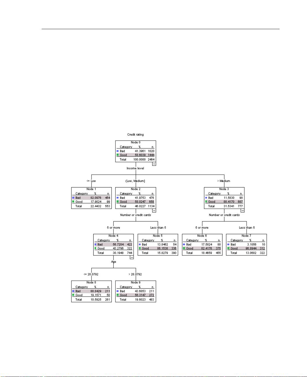
Figure 1-1

Classification tree

ssification Trees

1

2

Chapter 1

The Classification Tree procedure creates a tree-based classification model. It
classifies cases into groups or predicts values of a dependent (target) variable based
on values of

independent (predictor) variables. The procedure provides validation

tools for exploratory and confirmatory classification analysis.

The procedure can be used for:

Segmentation. Identify persons who are likely to be members of a particular group.
Stratification. Assign cases into one of several categories, such as high-, medium-, and

low-risk g

Prediction. Create rules and use them to predict future events, such as the likelihood

roups.

that someone will default on a loan or the potential resale value of a vehicle or home.

Data reduc

tion and variable screen ing.

Select a useful subset of predictors from a large

set of variables for use in building a formal parametric model.

Interaction identificat ion. Identify relationships that pertain only to specific subgroups

and specif

Category merging and discretizing continuous variables. Recode group predictor

y these in a formal parametric model.

categories and continuous variables with minimal loss of information.

Example. A bank wants to categorize credit applicants according to whether or not

they repr

esent a reasonable credit risk. Based on various factors, including the known
credit ratings of past customers, you can build a model to predict if future customers
are likely to default on their loans.

A tree-based analysis provides some attractive features:

 It allows you to identify homogeneous groups with high or low risk.
 It makes it easy to construct rules for making predictions about individual cases.

3

Creating Class

Data Considerations

The dependent and independent variables can be:

Data.

 Nominal. A variable can be treated as nominal when its values represent categories

with no intri

nsic ranking; for example, the department of the company in which

ification Trees

an employee works. Examples of nominal variables include region, zip code, or
religious affiliation.

 Ordinal. A variable can be treated as ordinal when its values represent categories

with some in

trinsic ranking; for example, levels of service satisfaction from
highly dissatisfied to highly satisfied. Examples of ordinal variables include
attitude scores representing degree of satisfaction or confidence and preference
rating sco

 Scale. Av

res.

ariable can be treated as scale when its values represent ordered
categories with a meaningful metric, so that distance comparisons between values
are appropriate. Examples of scale variables include age in years and income in
thousand

Frequenc

sofdollars.

y weights

If weighting is in effect, fractional weights are rounded to the
closest integer; so, cases with a weight value of less than 0.5 are assigned a weight of
0 and are therefore excluded from the analysis.

Assumptions. This procedure assumes that the appropriate measurement level has

been ass

igned to all analysis variables, and some features assume that all values of the

dependent variable included in the analysis have defined value labels.

 Measurement level. Measurement level affects the tree computations; so, all

es should be assigned the appropriate measurement level. By default,

variabl
SPSS assumes that numeric variables are scale and string variables are nominal,
which may not accurately reflect the true measurement level. An icon next to
each va

riable in the variable list identifies the variable type.

4

Chapter 1

Scale

Nominal

Ordinal

You can temporarily change the measurement level for a variable by right-clicking
the variable in the source variable list and selecting a measurement level from the
context menu.

 Value labels. The dialog box interface for this procedure assumes that either all

nonmissing values of a categorical (nominal, ordinal) dependent variable have
defined value labels or none of them do. Some features are not available unless at
least two nonmissing values of the categorical dependent variable have value
labels. If at least two nonmissing values have defined value labels, any cases with
other values that do not have value labels will be excluded from the analysis.

To Obtain Classification Trees

E From the menus choose:

Analyze

Classify

Tree...

5

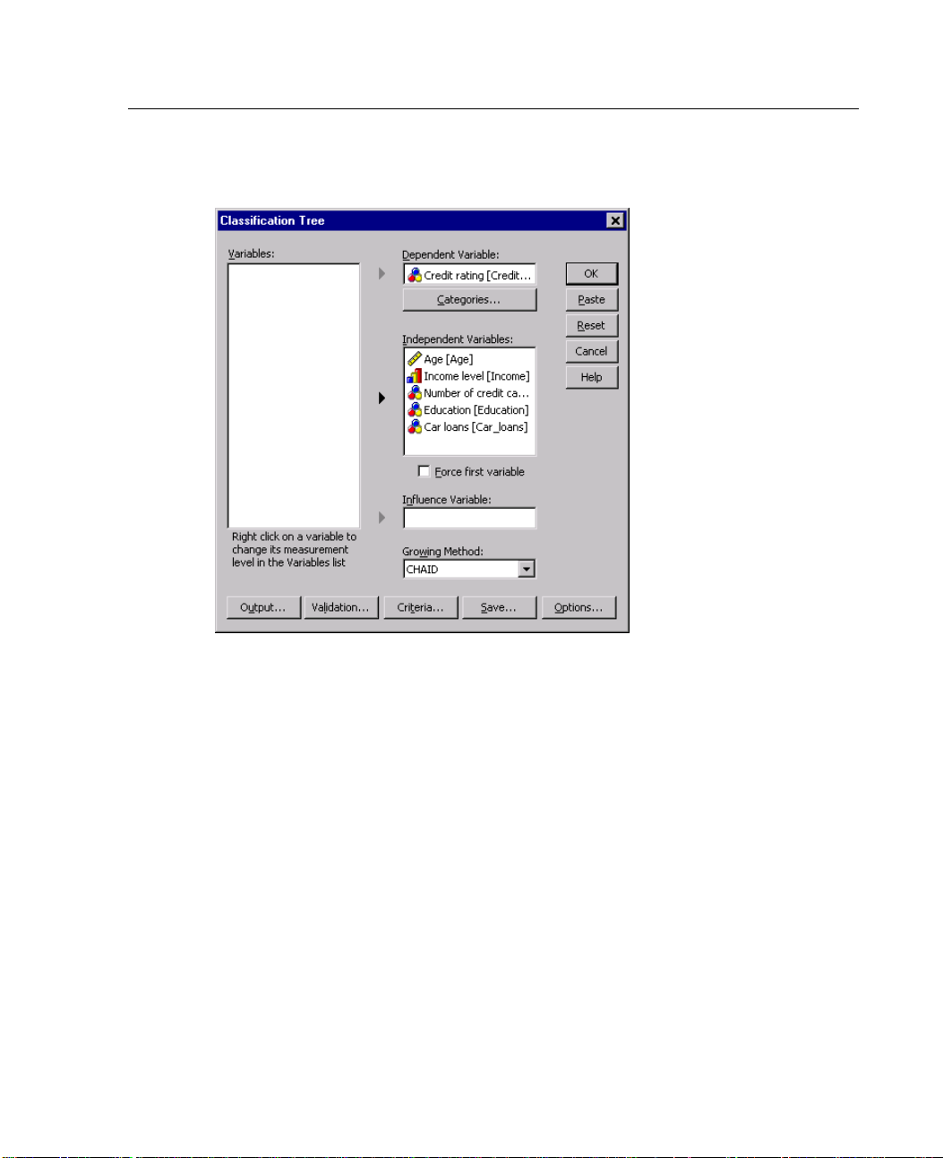
Figure 1-2

Classification Tree dialog box

Creating Class

ification Trees

E Select a dependent variable.
E Select one or more independent variables.
E Select a growing method.

Optionally, you can:

 Change the measurement level for any variable in the source list.
 Force the first variable in the independent variables list into the model as the

first split variable.

 Select an influence variable that defines how much influence a case has on the

rowing process. Cases with lower influence values have less influence;

tree-g
cases with higher values have more. Influence variable values must be positive.

 Validate the tree.
 Customize the tree-growing criteria.

6

Chapter 1



Save terminal node numbers, predicted values, and predicted probabilities

as variable

 Save the mod

Changing Measurement Level

E Right-click the variable in the source list.
E Select a measurement level from the pop-up context menu.

s.

el in XML (PMML) format.

This change

s the measurement level temporarily for use in the Classification Tree

procedure.

Growing Met

The availab

CHAID. Chi-squared Automatic Interaction Detection. At each step, CHAID

hods

le growing methods are:

chooses the independent (predictor) variable that has the strongest interaction with
the depend

ent variable. Categories of each predictor are merged if they are not

significantly different with respect to the dependent variable.

Exhaustive CHAID. A modification of CHAID that examines all possible splits for

each predi

CRT. Classification and Regression Trees. CRT splits the data into segments that are

ctor.

as homogeneous as possible with respect to the dependent variable. A terminal node
in which a

ll cases have the same value for the dependent variable is a homogeneous,

"pure" node.

QUEST. Quick, Unbiased, Efficient Statistical Tree. A method that is fast and avoids

other met

hods' bias in favor of predictors with many categories. QUEST can be

specified only if the dependent variable is nominal.

There are benefits and limitations with each method, including:

CHAID* CRT QUEST

Chi-square-based** X
Surrogate independent (predictor)

variables

XX

7

Tree pruning X X
Multiway node splitting X
Binary node splitting X X
Influence variables X X
Prior probabilities X X
Misclassification costs X X X
Fast calculation X X

*Includes Exhaustive CHAID.
**QUEST also uses a chi-square measure for nominal independent variables.

Selecting Categories

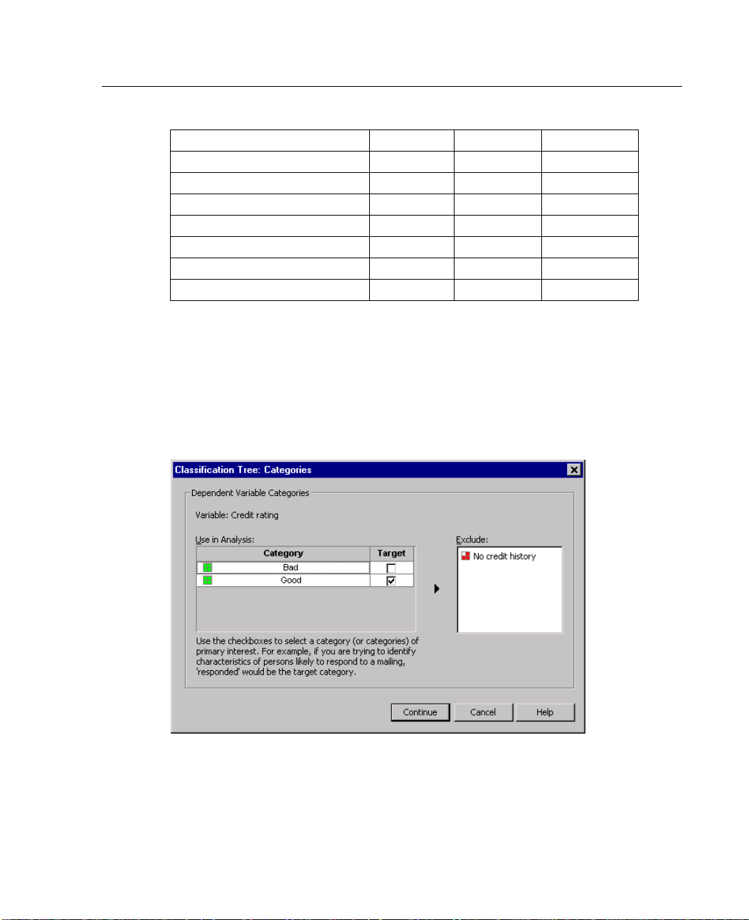
Figure 1-

Categori

3

es dialog box

Creating Class

CHAID* CRT QUEST

ification Trees

ategorical (nominal, ordinal) dependent variables, you can:

For c

 Con
 Ide

trol which categories are included in the analysis.

ntify the target categories of interest.

8

Chapter 1

Including/Excluding Categories

You can limit the analysis to specific categories of the dependent variable.

 Cases with values of the dependent variable in the Exclude list are not included

in the analys

 For nominal

is.

dependent variables, you can also include user-missing categories in
the analysis. (By default, user-missing categories are displayed in the Exclude
list.)

Tar get Cat e

Selected (c

gories

hecked) categories are treated as the categories of primary interest in the
analysis. For example, if you are primarily interested in identifying those individuals
most likely to default on a loan, you might select the “bad” credit-rating category
as the targ

 There is n

et category.

o default target category. If no category is selected, some classification

rule options and gains-related output are not available.

 If multiple categories are selected, separate gains tables and charts are produced

for each target category.

 Designating one or more categories as target categories has no effect on the tree

model, ri

Categories and Value Labels

sk estimate, or misclassification results.

This dialog box requires defined value labels for the dependent variable. It is not
availabl

e unless at least two values of the categorical dependent variable have defined

value labels.

To Inclu d

E In the ma

e/Exclude Categories and Select Target Categories

in Classification Tree dialog box, select a categorical (nominal, ordinal)

dependent variable with two or more defined value labels.

E Click Categories.

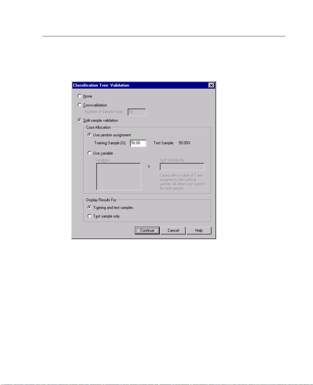
9

Validation

Figure 1-4

Validation dialog box

Creating Class

ification Trees

Validation allows you to assess how well your tree structure generalizes to a larger
population. Two validation methods are available: crossvalidation and split-sample

ation.

valid

Crossvalidation

Crossvalidation divides the sample into a number of subsamples, or folds.Tree

ls are then generated, excluding the data from each subsample in turn. The first

mode
tree is based on all of the cases except those in the first sample fold, the second tree
is based on all of the cases except those in the second sample fold, and so on. For

tree, misclassification risk is estimated by applying the tree to the subsample

each
excluded in generating it.

10

Chapter 1



You can specify a maximum of 25 sample folds. The higher the value, the fewer

the number o

 Crossvalid

f cases excluded for each tree model.

ation produces a single, final tree model. The crossvalidated risk
estimate for the final tree is calculated as the average of the risks for all of the
trees.

Split-Samp

With split-

le Validation

sample validation, the model is generated using a training sample and

tested on a hold-out sample.

 You can specify a training sample size, expressed as a percentage of the total

sample siz

 If you use

e, or a variable that splits the sample into training and testing samples.

a variable to define training and testing samples, cases with a value
of 1 for the variable are assigned to the training sample, and all other cases are
assigned to the testing sample. The variable cannot be the dependent variable,
weight var

 You can di

iable, influence variable, or a forced independent variable.

splay results for both the training and testing samples or just the
testing sample.

 Split-sample validation should be used with caution on small data files (data files

with a small number of cases). Small training sample sizes may yield poor
models, s

ince there may not be enough cases in some categories to adequately

grow the tree.

Tree-Growing Criteria

The available growing criteria may depend on the growing method, level of
measurement of the dependent variable, or a combination of the two.

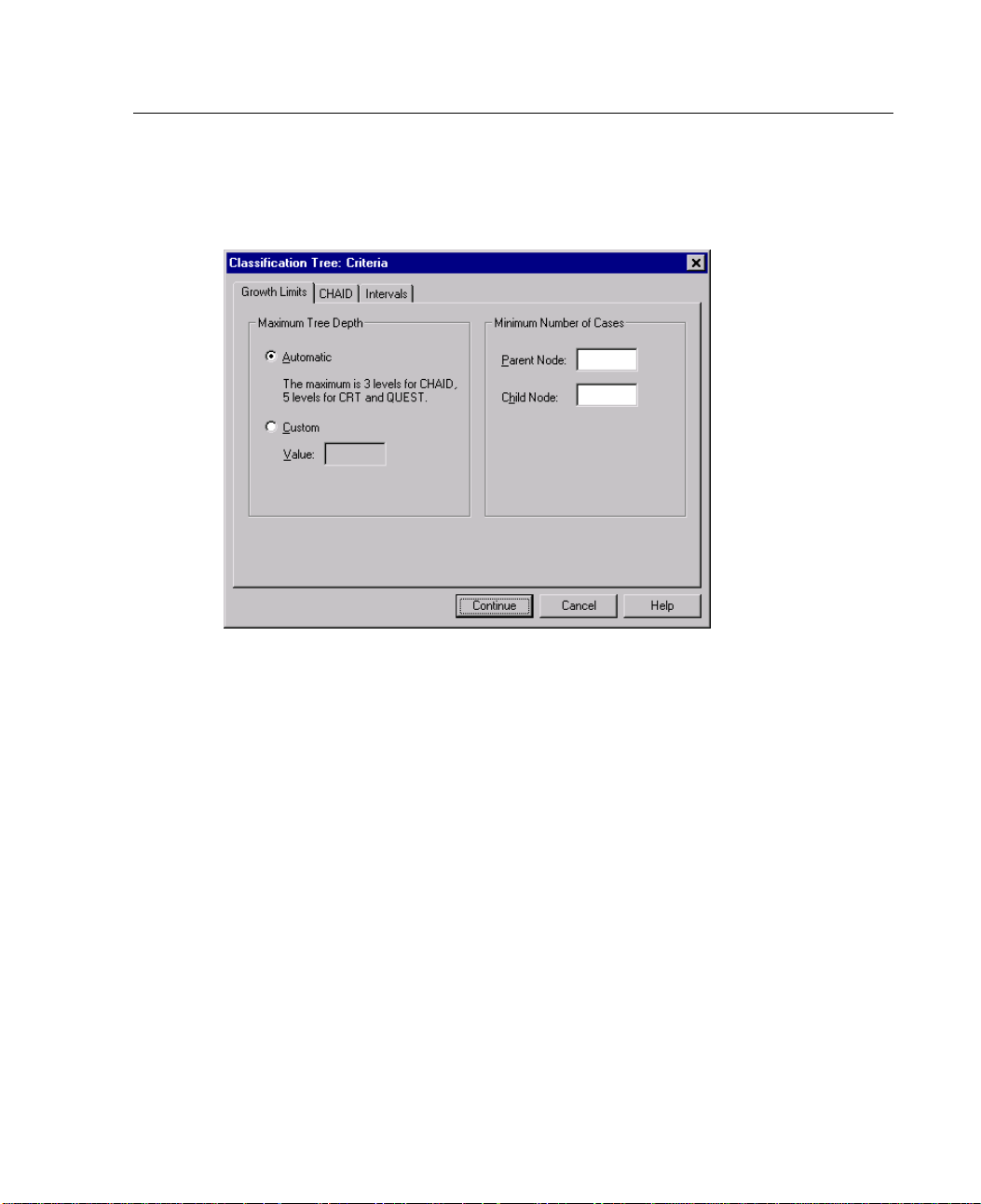
11

Growth Limits

Figure 1-5

Criteria dia

logbox,GrowthLimitstab

Creating Class

ification Trees

The Growth Limits tab allows you to limit the number of levels in the tree and control
the minimum number of cases for parent and child nodes.

Maximum Tree Depth. Controls the maximum number of levels of growth beneath

the roo

tnode.The

Automatic setting limits the tree to three levels beneath the root

node for the CHAID and Exhaustive CHAID methods and five levels for the CRT
and QUEST methods.

Minimum Number of Cases. Controls the minimum numbers of cases for nodes. Nodes

o not satisfy these criteria will not be split.

that d

 Incr
 Decr

easing the minimum values tends to produce trees with fewer nodes.

easing the minimum values produces trees with more nodes.

For data files with a small number of cases, the default values of 100 cases for parent
nodes and 50 cases for child nodes may sometimes result in trees with no nodes

the root node; in this case, lowering the minimum values may produce more

below
useful results.

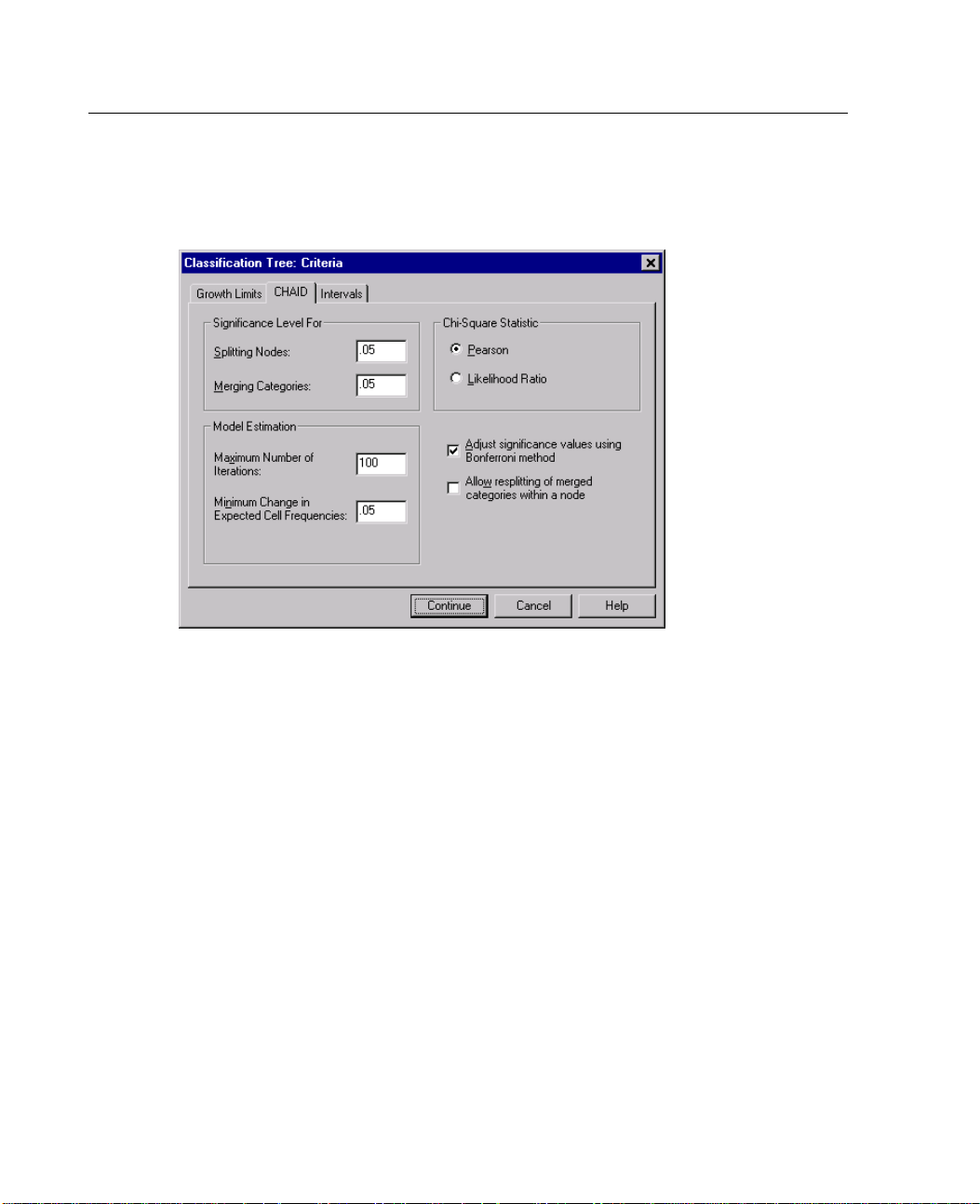
12

Chapter 1

CHAID Criteria

Figure 1-6

Criteria dia

log box, CHAID tab

For the CHAID and Exhaustive CHAID methods, you can control:

Significance Level. You can control the significance value for splitting nodes and

merging categories. For both criteria, the default significance level is 0.05.

 For splitting nodes, the value must be greater than 0 and less than 1. Lower values

tend to produce trees with fewer nodes.

 For merging categories, the value must be greater than 0 and less than or equal to

1. To pr

event merging of categories, specifyavalueof1.Forascaleindependent
variable, this means that the number of categories for the variable in the final tree
is the specified number of intervals (the default is 10). For more information,

cale Intervals for CHAID Analysis” on p. 14.

see “S

13

Creating Class

Chi-Square Statistic. For ordinal dependent variables, chi-square for determining node

ification Trees

splitting and category merging is calculated using the likelihood-ratio method. For
nominal dep

 Pearson. T

endent variables, you can select the method:

his method provides faster calculations but should be used with caution

on small samples. This is the default method.

 Likelihood ratio. This method is more robust that Pearson but takes longer to

calculate. For small samples, this is the preferred method.

Model Estimation. For nominal and ordinal dependent variables, you can specify:

 Maximum number of iterations. The default is 100. If the tree stops growing

because the

maximum number of iterations has been reached, you may want to
increase the maximum or change one or more of the other criteria that control
tree growth.

 Minimum change in expected cell frequencies. The value must be greater than 0

and less th

an 1. The default is 0.05. Lower values tend to produce trees with

fewer nodes.

Adjust significance values using B onferroni method. For multiple comparisons,

signific

ance values for merging and splitting criteria are adjusted using the Bonferroni

method. This is the default.

Allow resplitting of merged categories within a node. Unless you explicitly prevent

category merging, the procedure will attempt to merge independent (predictor)
variable

categories together to produce the simplest tree that describes the model.
This option allows the procedure to resplit merged categories if that provides a better
solution.

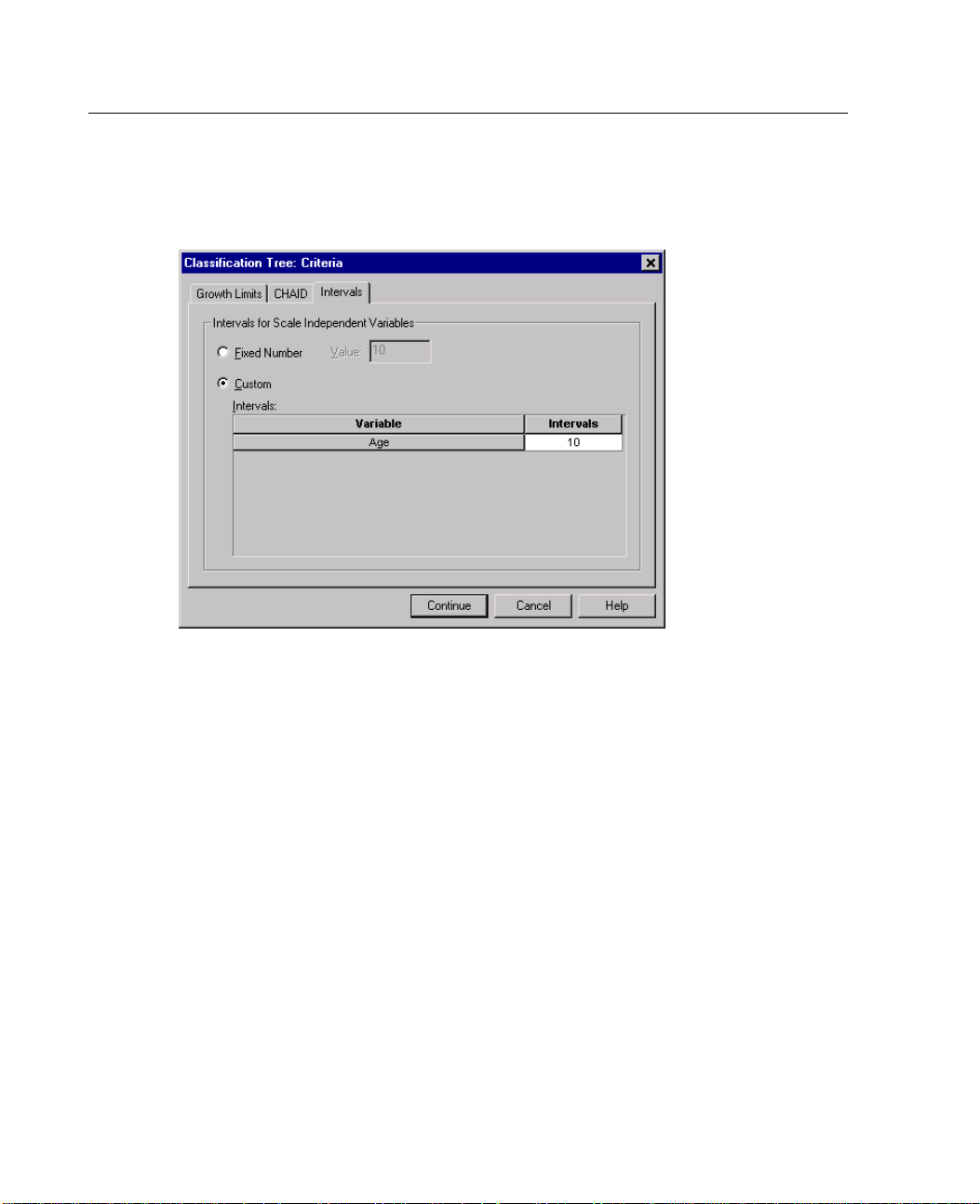
14

Chapter 1

Scale Intervals for CHAID Analysis

Figure 1-7

Criteria dia

log box, Intervals tab

In CHAID analysis, scale independent (predictor) variables are always banded into
discrete groups (for example, 0–10, 11–20, 21–30, etc.) prior to analysis. You can

l the initial/maximum number of groups (although the procedure may merge

contro
contiguous groups after the initial split):

 Fixed number. All scale independent variables are initially banded into the same

number

 Custo

of groups. The default is 10.

m.

Each scale independent variable is initially banded into the number

of groups specified for that variable.

To Specify Intervals for Scale Independent Variables

E In the main Classification Tree dialog box, select one or more scale independent

variables.

E For the growing method, select CHAID or Exhaustive CHAID.
E Click Criteria.

15

E

Click the Intervals tab.
In CRT and QUEST analysis, all splits are binary and scale and ordinal independent

variables a
for scale independent variables.

CRT Criteri

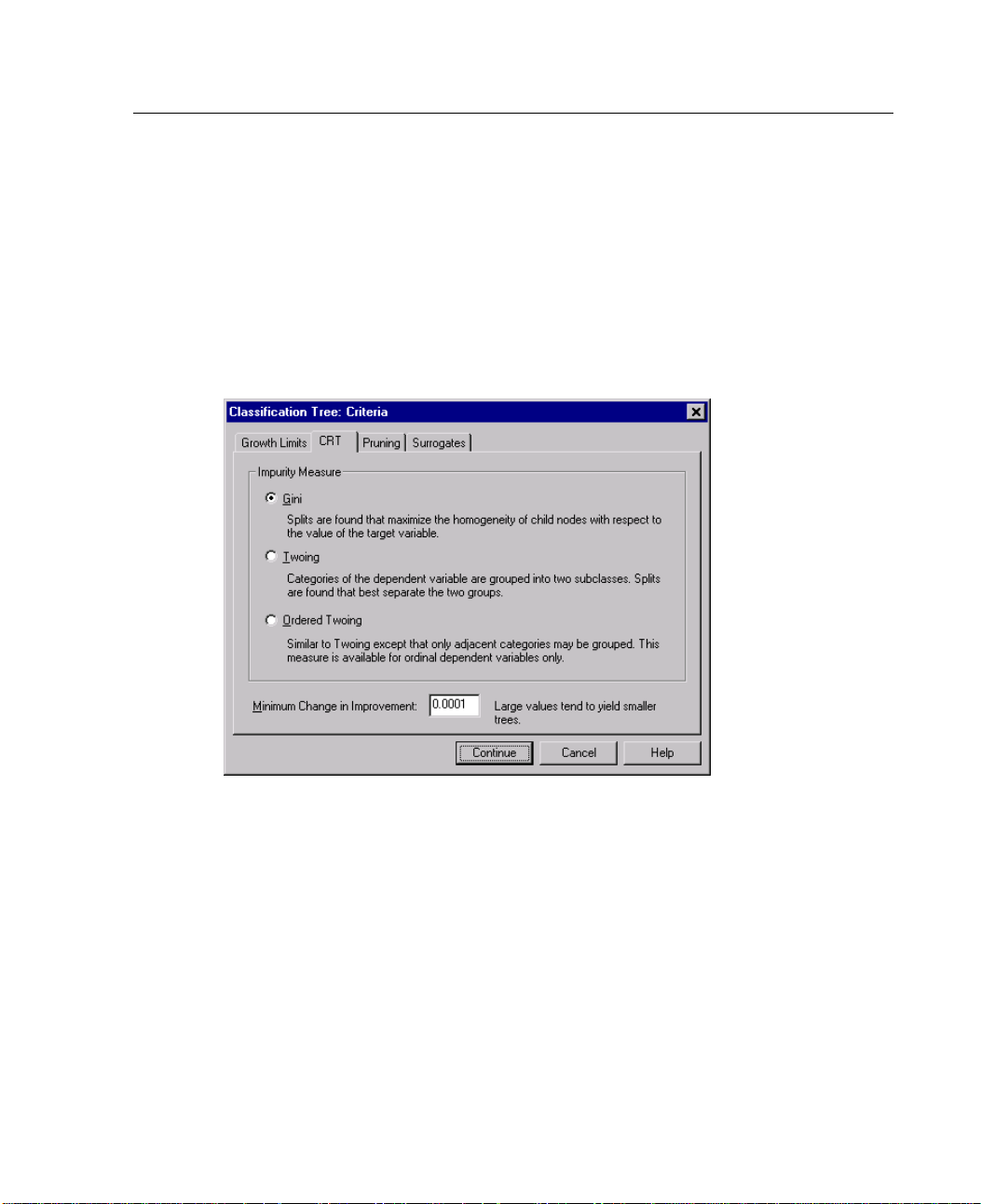
Figure 1-8

Criteria dialog box, CRT tab

Creating Class

ification Trees

re handled the same way; so, you cannot specify a number of intervals

a

The CRT growing method attempts to maximize within-node homogeneity. The
extent to which a node does not represent a homogenous subset of cases is an
indication of impurity. For example, a terminal node in which all cases have the
same value for the dependent variable is a homogenous node that requires no further
splitting because it is “pure.”

You can select the method used to measure impurity and the minimum decrease in

impurity required to split nodes.

Impurity M easure. For scale dependent variables, the least-squared deviation (LSD)

measure of impurity is used. It is computed as the within-node variance, adjusted for
any frequency weights or influence values.

16

Chapter 1

For categorical (nominal, ordinal) dependent variables, you can select the impurity
measure:

 Gini. Splits are found that maximize the homogeneity of child nodes with respect

to the value of the dependent variable. Gini is based on squared probabilities
of membersh

ip for each category of the dependent variable. It reaches its
minimum (zero) when all cases in a node fall into a single category. This is
the default measure.

 Twoing. Categories of the dependent variable are grouped into two subclasses.

Splits are

 Ordered t

found that best separate the two groups.

woing.

Similar to Twoing except that only adjacent categories can be

grouped. This measure is available only for ordinal dependent variables.

Minimum cha nge in improvement. This is the minimum decrease in impurity required

to split a n

ode. The default is 0.0001. Higher values tend to produce trees with

fewer nodes.

QUEST Cri

teria

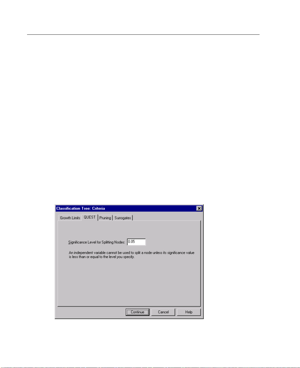
Figure 1-9

Criteria dialog box, QUEST tab

17

E In the main Classification Tree dialog box, select a nominal dependent variable.
E For the growing method, select QUEST.
E Click Criteria.
E Click the QUEST tab.

Pruning Tr

Creating Class

ification Trees

For the QUEST method, you can specify the significance level for splitting nodes. An
independent variable cannot be used to split nodes unless the significance level is
less than or

equal to the specified value. The value must be greater than 0 and less
than 1. The default is 0.05. Smaller values will tend to exclude more independent
variables from the final model.

To Specify QUEST Criteria

ees

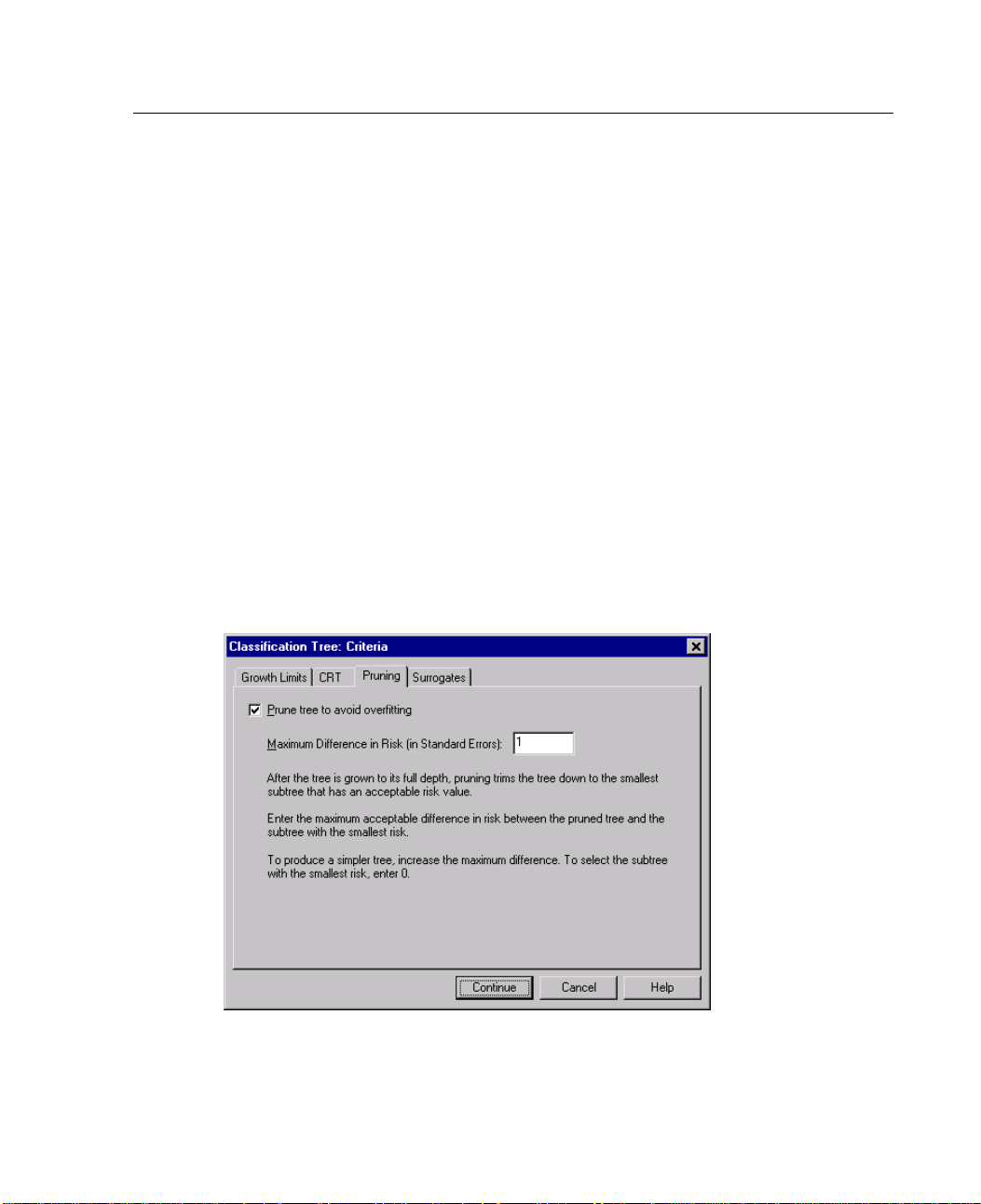
Figure 1-10

Criteria dialog box, Pruning tab

18

Chapter 1

With the CRT and QUEST methods, you can avoid overfitting the model by pruning
the tree: the tree is grown until stopping criteria are met, and then it is trimmed
automatica

lly to the smallest subtree based on the specified maximum difference in
risk. The risk value is expressed in standard errors. The default is 1. The value must
be non-negative. To obtain the subtree with the minimum risk, specify 0.

Pruning versus Hiding Nodes

When you create a pruned tree, any nodes pruned from the tree are not available in
the final tree. You can interactively hide and show selected child nodes in the final
tree, but y

ou cannot show nodes that were pruned in the tree creation process. For

more information, see “Tree Editor” in Chapter 2 on p. 49.

Surrogat

es

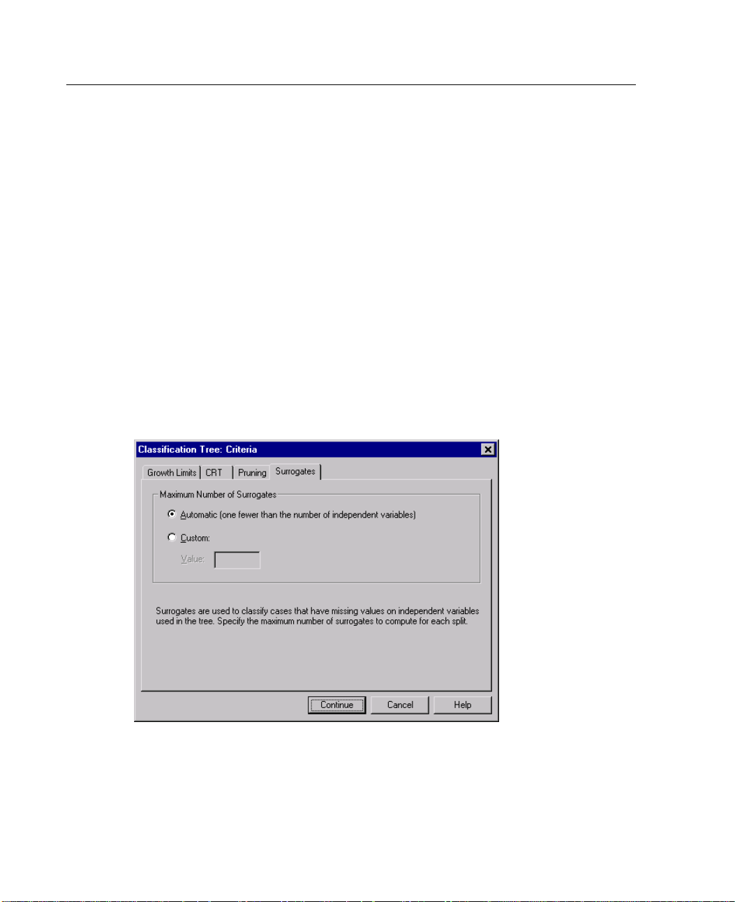
Figure 1-11

Criteria dialog box, Surrogates tab

CRTandQUESTcanusesurrogates for independent (predictor) variables. For cases in which the value for that variable is missing, other independent variables having high associations with the original variable are used for classification. These

19

alternative predictors are called surrogates. You can specify the maximum number of
surrogates to use in the model.

 By default, the maximum number of surrogates is one less than the number of

independent variables. In other words, for each independent variable, all other
independen

 If you don’

t variables may be used as surrogates.

t want the model to use surrogates, specify 0 for the number of

surrogates.

Options

Available options may depend on the growing method, the level of measurement of
the dependent variable, and/or the existence of defined value labels for values of
the depend

Misclassification Costs

Figure 1-12

Options dialog box, Misclassification Costs tab

ent variable.

Creating Class

ification Trees

20

Chapter 1

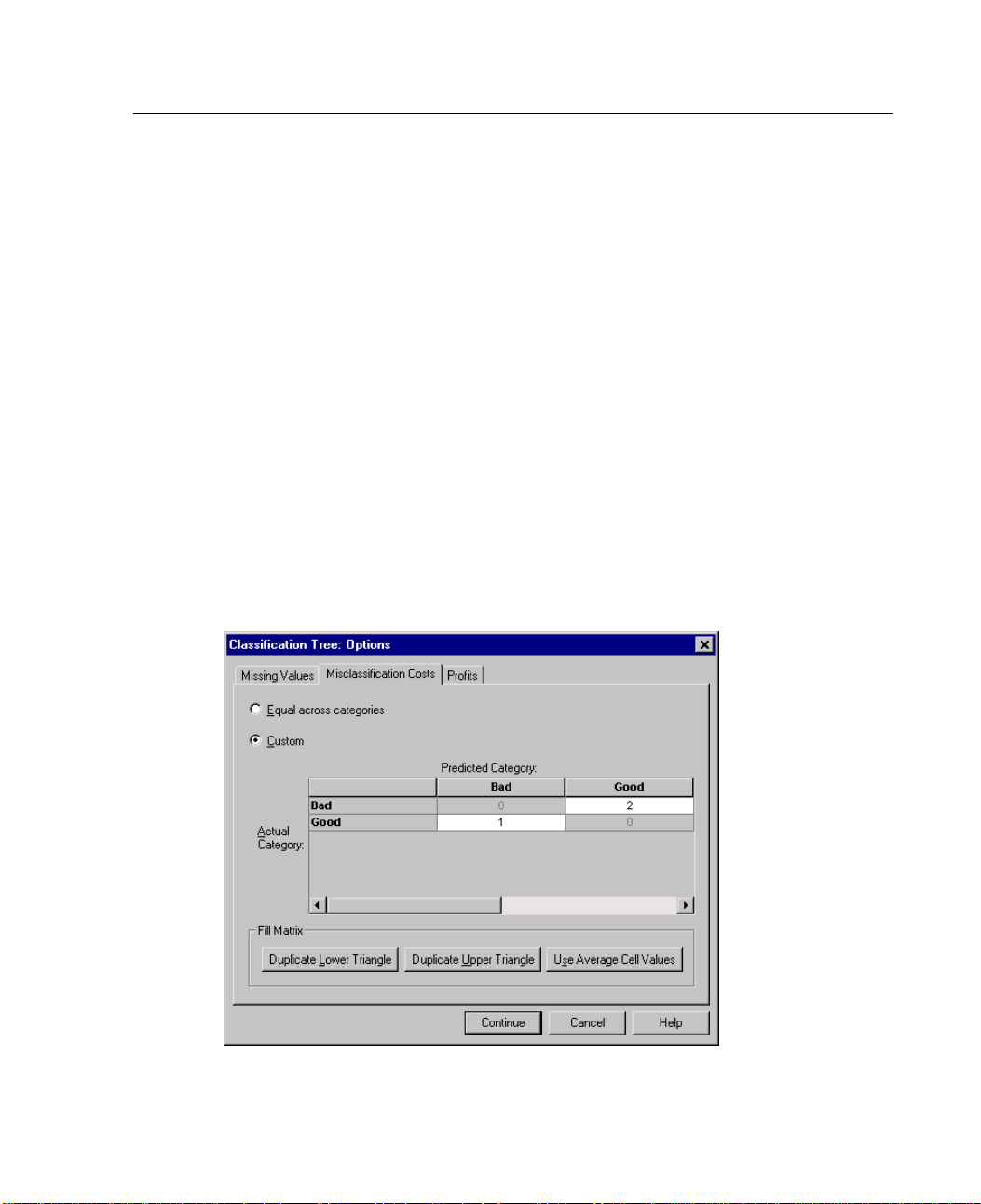
For categorical (nominal, ordinal) dependent variables, misclassification costs allow
you to include information about the relative penalty associated with incorrect
classifica

 The cost of

tion. For example:

denying credit to a creditworthy customer is likely to be different

from the cost of extending credit to a customer who then defaults on the loan.

 Thecostofmisclassifyinganindividual with a high risk of heart disease as

low risk is probably much higher than the cost of misclassifying a low-risk
individual

 The cost of

as high-risk.

sendingamassmailingtosomeonewhoisn’tlikelytorespondis
probably fairly low, while the cost of not sending the mailing to someone who is
likely to respond is relatively higher (in terms of lost revenue).

Misclassi

This dialo

fication Costs and Value Labels

g box is not available unless at least two values of the categorical dependent

variable have defined value labels.

To Specify

E In the ma

Misclassification Costs

in Classification Tree dialog box, select a categorical (nominal, ordinal)

dependent variable with two or more defined value labels.

E Click Options.
E Click the Misclassification Costs tab.
E Click Custom.
E Enter one or more misclassification costs in the grid. Values must be non-negative.

(Correct classifications, represented on the diagonal, are always 0.)

Fill Matrix. In many instances, you may want costs to be symmetric—that is, the

cost of m

isclassifying A as B is the same as the cost of misclassifying B as A. The

following controls can make it easier to specify a symmetric cost matrix:

 Duplicate Lower Triangle. Copies values in the lower triangle of the matrix (below

the diag

onal) into the corresponding upper-triangular cells.

21

Profits

Creating Class



Duplicate Upper Triangle. Copies values in the upper triangle of the matrix (above

the diagona

 Use Average

l) into the corresponding lower-triangular cells.

Cell Values.

For each cell in each half of the matrix, the two values

ification Trees

(upper- and lower-triangular) are averaged and the average replaces both
values. For example, if the cost of misclassifying A as B is 1 and the cost of
misclassif

ying B as A is 3, then this control replaces both of those values with the

average (1+3)/2 = 2.

Figure 1-1

Options di

3

alog box, Profits tab

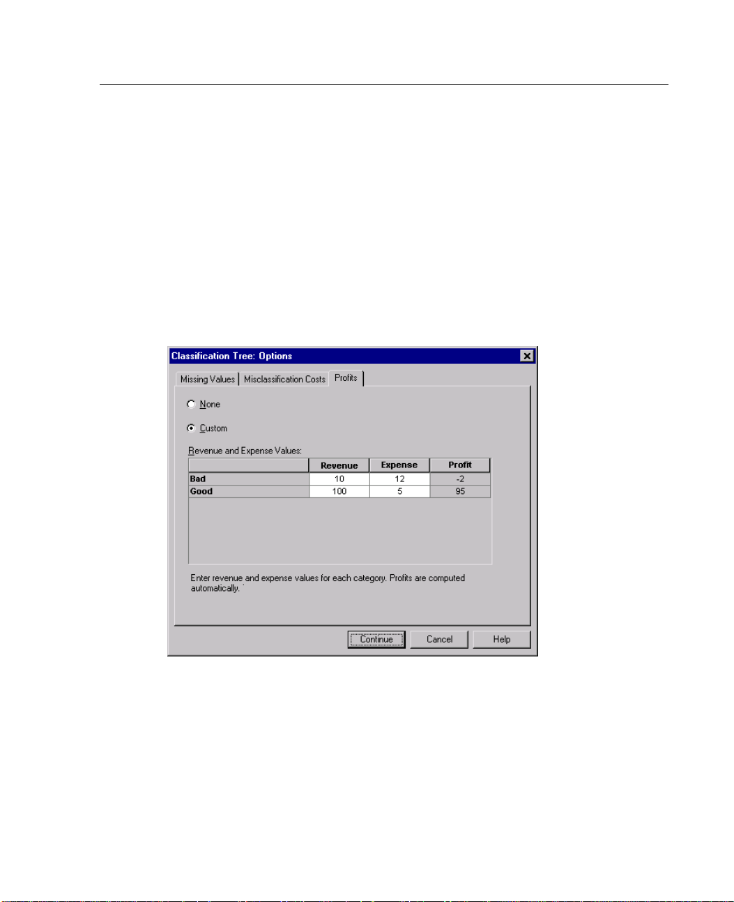
For categorical dependent variables, you can assign revenue and expense values to

s of the dependent variable.

level

 Prof

it is computed as revenue minus expense.

22

Chapter 1



Profit values affect average profit and ROI (return on investment) values in gains

tables. The

 Revenue and

y do not affect the basic tree model structure.

expense values must be numeric and must be specified for all

categories of the dependent variable displayed in the grid.

Profits and Value Labels

This dialog box requires defined value labels for the dependent variable. It is not
available unless at least two values of the categorical dependent variable have defined
value labe

ls.

To Specify Profits

E In the main Classification Tree dialog box, select a categorical (nominal, ordinal)

dependent

E Click Opt

variable with two or more defined value labels.

.

ions

E Click the
E Click Cus
E Enter rev

the grid.

Profits tab.

.

tom

enue and expense values for all dependent variable categories listed in

23

Prior Probabilities

Figure 1-14

Options dial

og box, Prior Probabilities tab

Creating Class

ification Trees

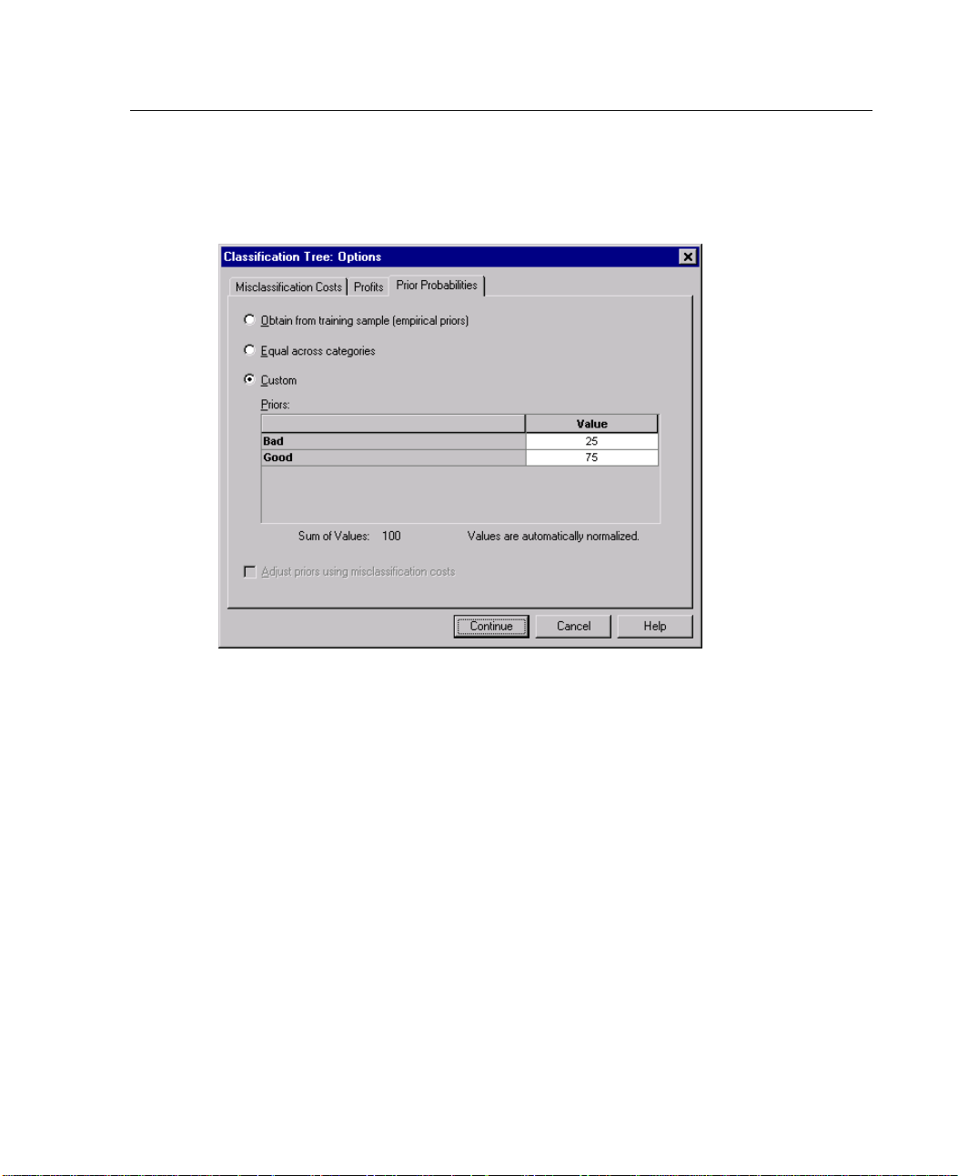
For CRT and QUEST trees with categorical dependent variables, you can specify

robabilities of group membership. Prior probabilities are estimates of

prior p
the overall relative frequency for each category of the dependent variable prior to
knowing anything about the values of the independent (predictor) variables. Using

probabilities helps to correct any tree growth caused by data in the sample that is

prior
not representative of the entire population.

Obtain from training sample (empirical priors). Use t his setting if the distribution

of dependent variable values in the data file is representative of the population

ibution. If you are using split-sample validation, the distribution of cases in the

distr
training sample is used.

Note: Since cases are randomly assigned to the training sample in split-sample

dation, you won’t know the actual distribution of cases in the training sample in

vali
advance. For more information, see “Validation” on p. 9.

24

Chapter 1

Equal across categories. Use this setting if categories of the dependent variable are

represented equally in the population. Forexample,iftherearefourcategories,
approximat

ely 25% of the cases are in each category.

Custom. Ent

er a non-negative value for each category of the dependent variable listed
in the grid. The values can be proportions, percentages, frequency counts, or any
other values that represent the distribution of values across categories.

Adjust priors using misclassification costs. If you define custom misclassification

costs, you

can adjust prior probabilities based on those costs. For more information,

see “Misclassification Costs” on p. 19.

Profits an

This dialo

d Value Labels

g box requires defined value labels for the dependent variable. It is not
available unless at least two values of the categorical dependent variable have defined
value labels.

To Specify Prior Probabilities

E In the main Classification Tree dialog box, select a categorical (nominal, ordinal)

dependent variable with two or more defined value labels.

E For the growing method, select CRT or QUEST.
E Click Options.
E Click the Prior Probabilities tab.

25

Scores

Figure 1-15

Options dial

og box, Scores tab

Creating Class

ification Trees

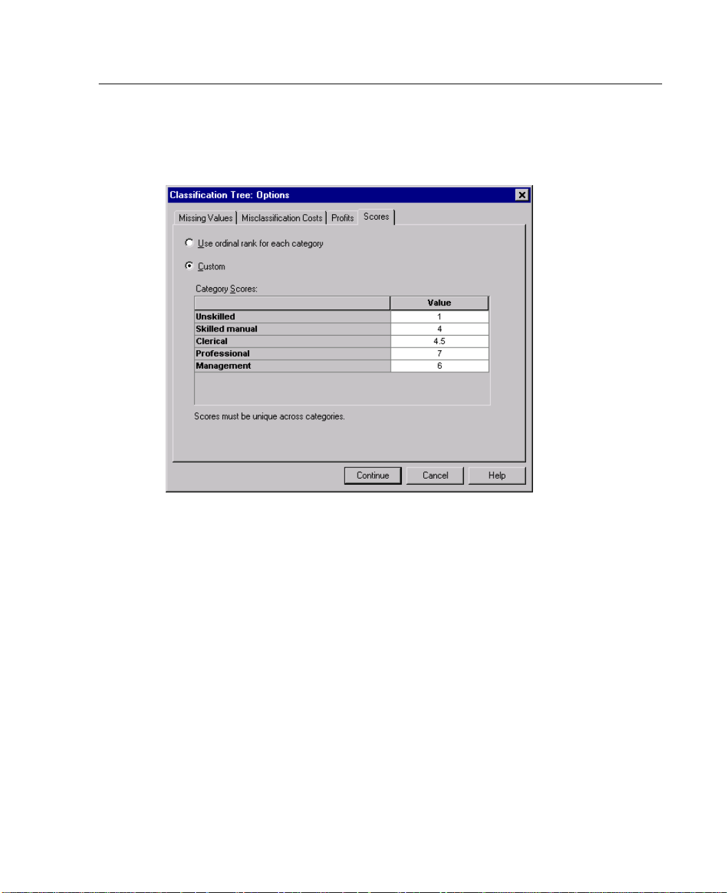
For CHAID and Exhaustive CHAID with an ordinal dependent variable, you can

custom scores to each category of the dependent variable. Scores define the

assign
order of and distance between categories of the dependent variable. You can use
scores to increase or decrease the relative distance between ordinal values or to

e the order of the values.

chang

 Use o

rdinal rank for each category.

The lowest category of the dependent variable
is assigned a score of 1, the next highest category is assigned a score of 2, and so
on. This is the default.

 Custom. Enter a numeric score value for each category of the dependent variable

d in the grid.

liste

26

Chapter 1

Example

Value Label Original Value Score

Unskilled 1 1
Skilled manual 2 4
Clerical 3
Professional 4 7
Management

5

4.5

6

 The scor

es increase the relative distance between Unskilled and Skilled manual

and decrease the relative distance between Skilled manual and Clerical.

 The scores reverse the order of Management and Professional.

Scores and Value Labels

This dialog box requires defined value labels for the dependent variable. It is not
available unless at least two values of the categorical dependent variable have defined
value la

bels.

To Specify Scores

E In the main Classification Tree dialog box, select an ordinal dependent variable

with two

E For the
E Click O
E Click t

or more defined value labels.

growing method, select

.

ptions

Scores tab.

he

CHAID or Exhaustive CHAID.

27

Missing Values

Figure 1-16

Options dial

og box, Missing Values t ab

Creating Class

ification Trees

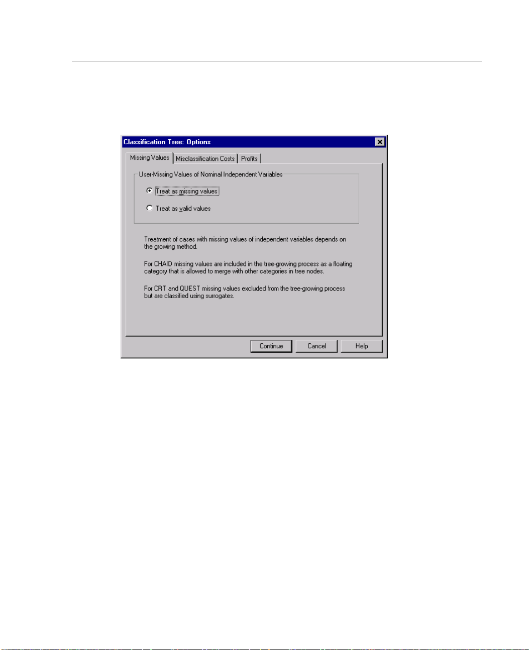
The Missing Values tab controls the handling of nominal, user-missing, independent

ctor) variable values.

(predi

 Handl

ing of ordinal and scale user-missing independent variable values varies

between growing methods.

 Handling of nominal dependent variables is specified in the Categories dialog

box. For more information, see “Selecting Categories” on p. 7.

 For ordinal and scale dependent variables, cases with system-missing or

issing dependent variable values are always excluded.

user-m

s missing values.

Treat a

User-missing values are treated like system-missing values.

The handling of system-missing values varies between growing methods.

Treat as valid values. User-missing values of nominal independent variablesare treated

as ordinary values in tree growing and classification.

28

Chapter 1

Method-Dependent Rules

If some, but not all, independent variable values are system- or user-missing:

 For CHAID and Exhaustive CHAID, system- and user-missing independent

variable val

ues are included in the analysis as a single, combined category. For
scale and ordinal independent variables, the algorithms first generate categories
using valid values and then decide whether to merge the missing category with its
most simila

 For CRT and

r (valid) category or keep it as a separate category.

QUEST, cases with missing independent variable values are
excluded from the tree-growing process but are classified using surrogates if
surrogates are included in the method. If nominal user-missing values are
treated as

missing, they are also handled in this manner. For more information,

see “Surrogates” on p. 18.

To Specify Nominal, Inde pen den t User-Missing Treatment

E In the main Classification Tree dialog box, select at least one nominal independent

variable.

E Click Options.
E Click the Missing Values tab.

29

Saving Model

Figure 1-17

Save dialog box

Information

Creating Class

ification Trees

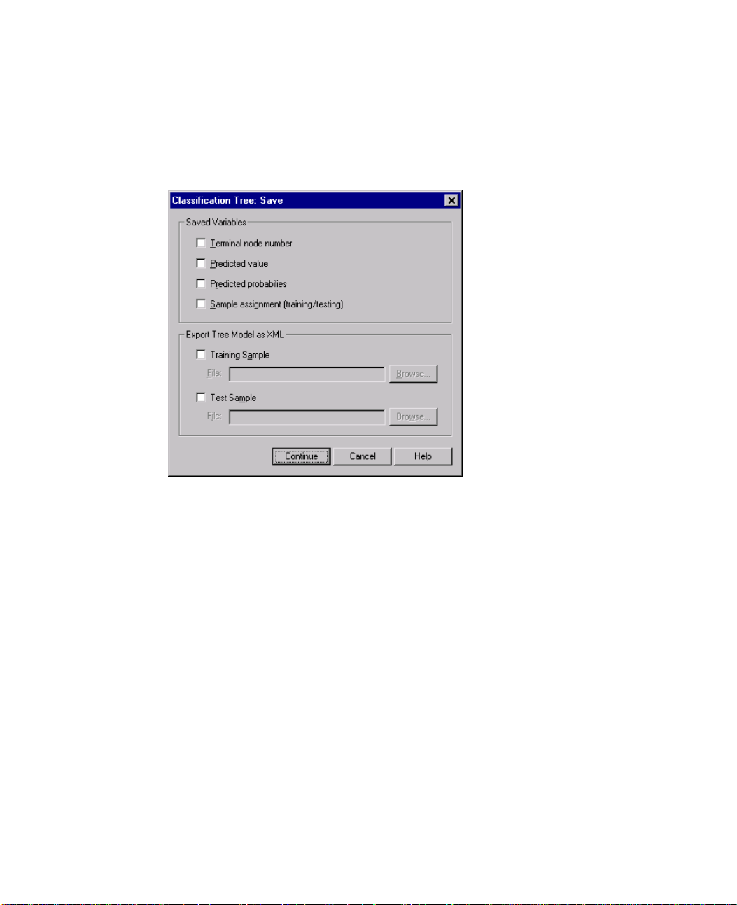
You can save information from the model as variables in the working data file, and
you can

Saved Variables

Term i n

also save the entire model in XML (PMML) format to an external file.

al node number.

The terminal node to which each case is assigned. The value is

thetreenodenumber.

Predicted value. The class (group) or value for the dependent variable predicted

by the m

Predicted probabilities. The probability associated with the model’s prediction. One

odel.

variable is saved for each category of the dependent variable. Not available for

dependent variables.

scale

Sample assignment (training/testing). For split-sample validation, this variable

indicates whether a case was used in the training or testing sample. The value is 1

etrainingsampleand0forthetestingsample. Not available unless you have

for th
selected split-sample validation. For more information, see “Validation” on p. 9.

30

Chapter 1

Output

Export Tree Model as XML

YoucansavetheentiretreemodelinXML (PMML) format. SmartScore and the
server version of SPSS (a separate product) can use this model file to apply the model
informatio

Training sa

n to other data files for scoring purposes.

mple.

Writes the model to the specified file. For split-sample validated

trees, this is the model for the training sample.

Test sampl e . Writes the model for the test sample to the specified file. Not available

unless you have selected split-sample validation.

Available output options depend on the growing method, the measurement level of
the dependent variable, and other settings.

31

Tree Display

Figure 1-18

Output dialo

gbox,Treetab

Creating Class

ification Trees

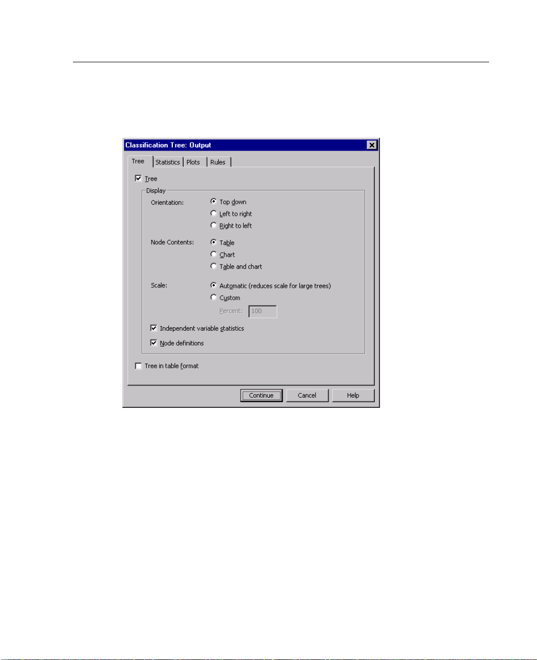
n control the initial appearance of the tree or completely suppress the tree

You ca
display.

Tree. By default, the tree diagram is included in the output displayed in the Viewer.

Deselect (uncheck) this option to exclude the tree diagram from the output.

Display. These options control the initial appearance of the tree diagram in the Viewer.

these attributes can also be modified by editing the generated tree.

All of

 Orie

ntation.

The tree can be displayed top down with the root node at the top,

left to right, or right to left.

32

Chapter 1



Node contents. Nodes can display tables, charts or both. For categorical dependent

variables,

tables display frequency counts and percentages, and the charts are bar
charts. For scale dependent variables, tables display means, standard deviations,
number of cases, and predicted values, and the charts are histograms.

 Scale. By default, large trees are automatically scaled down in an attempt to fit

the tree on t

 Independe

he page. You can specify a custom scale percentage of up to 200%.

nt variable statistics.

For CHAID and Exhaustive CHAID, statistics
include F value (for scale dependent variables) or chi-square value (for
categorical dependent variables) as well as significance value and degrees of
freedom. F

or CRT, the improvement value is shown. For QUEST, F, significance
value, and degrees of freedom are shown for scale and ordinal independent
variables; for nominal independent variables, chi-square, significance value,
and degre

 Node def

es of freedom are shown.

initions.

Node definitions display the value(s) of the independent variable

used at each node split.

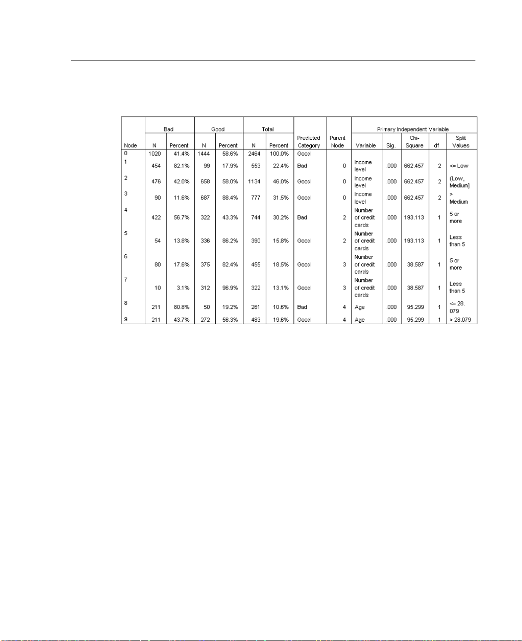
Tree in table format. Summary information for each node in the tree, including parent

node numb

er, independent variable statistics, independent variable value(s) for the
node, mean and standard deviation for scale dependent variables, or counts and
percentages for categorical dependent variables.

33

Figure 1-19

Tree in table format

Creating Class

ification Trees

34

Chapter 1

Statistics

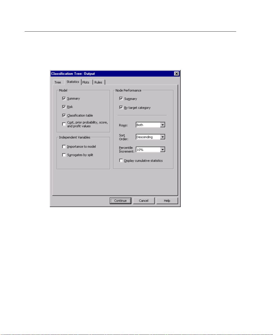
Figure 1-20

Output dialo

g box, Statistics tab

able statistics tables depend on the measurement level of the dependent variable,

Avail
the growing method, and other settings.

Model

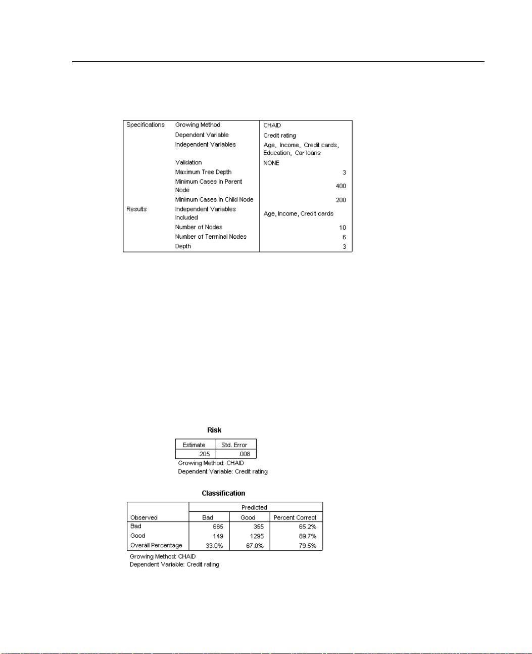
The summary includes the method used, the variables included in the

ry.

Summa

model, and the variables specified but not included in the model.

35

ification Trees

Figure 1-21

Model summary table

Risk. Ris

 For cate

k estimate and its standard error. A measure of the tree’s predictive accuracy.

gorical dependent variables, the risk estimate is the proportion of cases

Creating Class

incorrectly classified after adjustment for prior probabilities and misclassification
costs.

 For scale dependent variables, the risk estimate is within-node variance.

Classification table. For categorical (nominal, ordinal) dependent variables, this table

shows the number of cases classified correctly and incorrectly for each category of
the depe

ndent variable. Not available for scale dependent variables.

Figure 1-22

Risk and classification tables

36

Chapter 1

Cost, prior probability, score, and profit values. For categorical dependent variables, this

table shows the cost, prior probability, score, and profit values used in the analysis.
Not availab

Independent Variables

le for scale dependent variables.

Importance to model.

variable ac

cording to its importance to the model. Not available for QUEST or

For the CRT growing method, ranks each independent (predictor)

CHAID methods.

Surrogates by split. For the CRT and QUEST growing methods, if the model includes

surrogate

s, lists surrogates for each split in the tree. Not available for CHAID

methods. For more information, see “Surrogates” on p. 18.

Node Perfo

Summary.

rmance

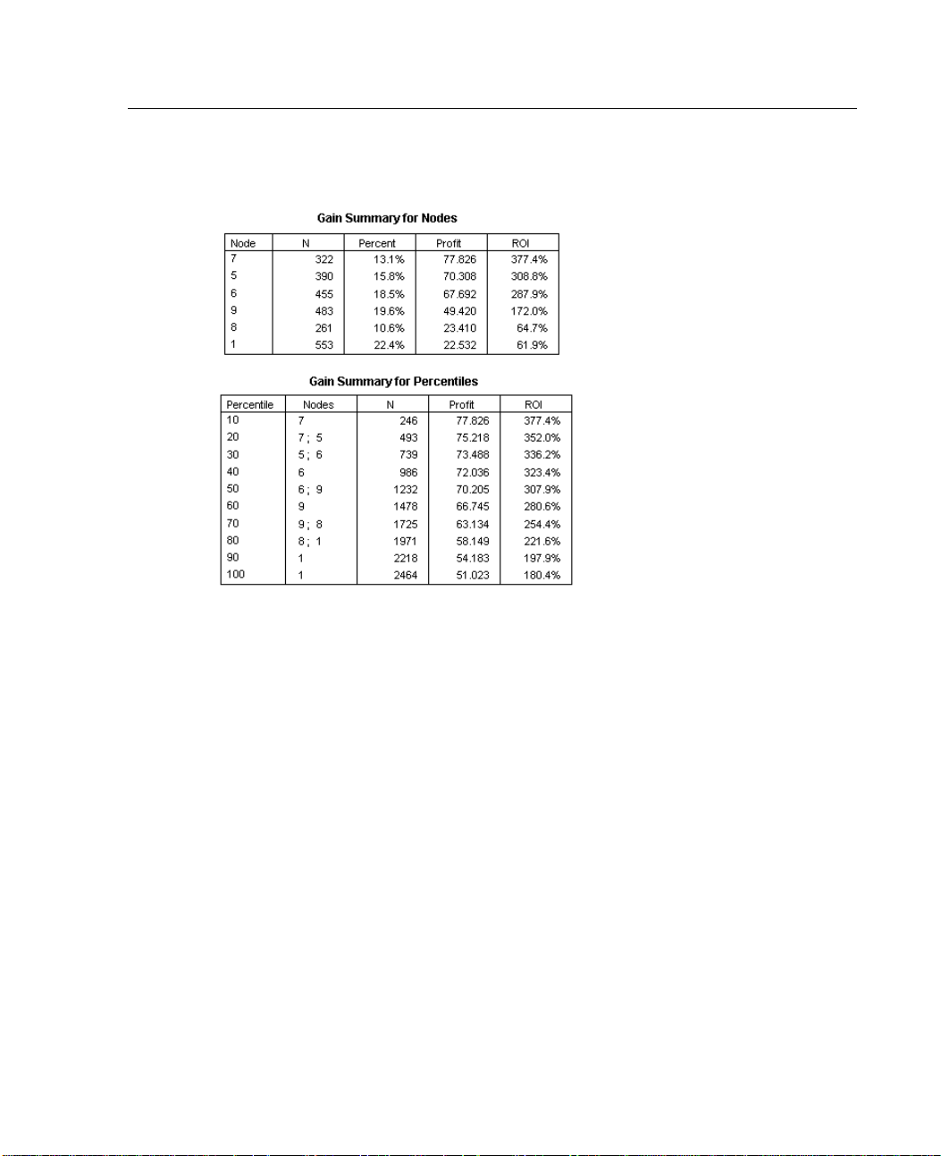
or scale dependent variables, the table includes the node number, the

F
number of cases, and the mean value of the dependent variable. For categorical
dependent variables with defined profits, the table includes the node number, the
number of

cases, the average profit, and the ROI (return on investment) values.
Not available for categorical dependent variables without defined profits. For more
information, see “Profits” on p. 21.

37

Creating Class

Figure 1-23

Gain summary tables for nodes and percentiles

ification Trees

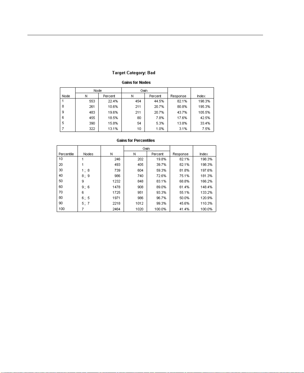
By target category. For categorical dependent variables with defined target categories,

the table includes the percentage gain, the response percentage, and the index
percentage (lift) by node or percentile group. A separate table is produced for each
target category. Not available for scale dependent variables or categorical dependent
variables without defined target categories. For more information, see “Selecting
Categories” on p. 7.

38

Chapter 1

Figure 1-24

Target category gains for nodes and percentiles

Rows. The node performance tables can display results by terminal nodes, percentiles,

or both. If you select both, two tables are produced for each targetcategory. Percentile

s display cumulative values for each percentile, based on sort order.

table

Percentile increment. For percentile tables, you can select the percentile increment:

1, 2, 5, 10, 20, or 25.

ay cumul ative statistics.

Displ

For terminal node tables, displays additional columns

in each table with cumulative results.

39

Charts

Figure 1-25

Output dialo

gbox,Plotstab

Creating Class

ification Trees

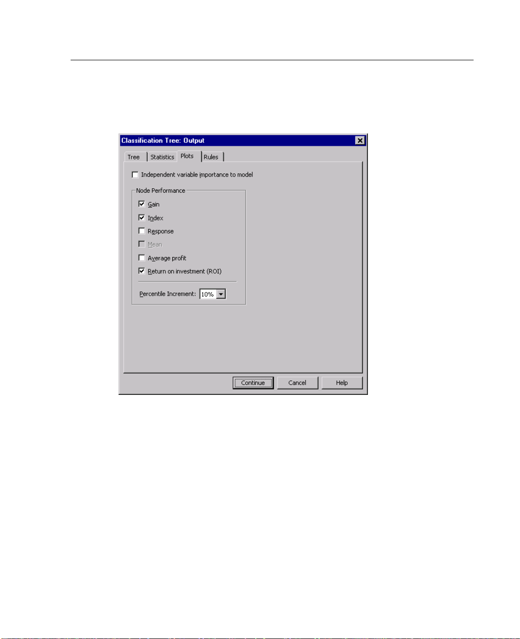
able charts depend on the measurement level of the dependent variable, the

Avail
growing method, and other settings.

Importance to model. Bar chart of model importance by independent variable

(predictor). Available only with the CRT growing method.

Node Performance

Gain is the percentage of total cases in the target category in each node,

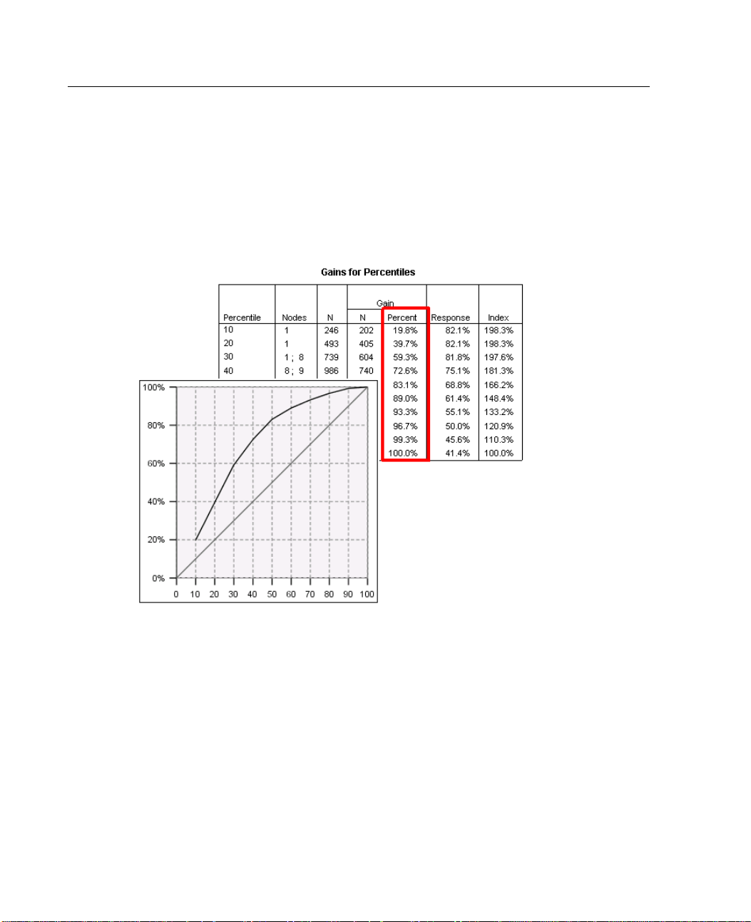
Gain.

computed as: (node target n/total target n) x 100. The gains chart is a line chart of

lative percentile gains, computed as: (cumulative percentile target n /total

cumu
target n) x 100. A separate line chart is produced for each target category. Available

40

Chapter 1

only for categorical dependent variables with defined target categories. For more
information, see “Selecting Categories” on p. 7.

The gains chart plots the same values that you would see in the Gain Percent column
in the gains

Figure 1-26

Gains for percentiles table and gains chart

for percentiles table, which also reports cumulative values.

Response. The percentage of cases in the node in the specified target category.

The response chart is a line chart of cumulative percentile response, computed as:
(cumulative percentile target n / cumulative percentile total n) x 100. Available only
for categorical dependent variables with defined target categories.

The response chart plots the same values that you would see in the Response column
in the gains for percentiles table.

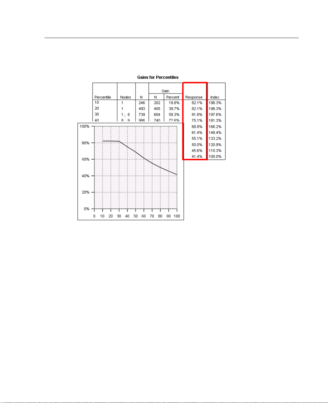
41

Figure 1-27

Gains for percentiles table and response chart

Creating Class

ification Trees

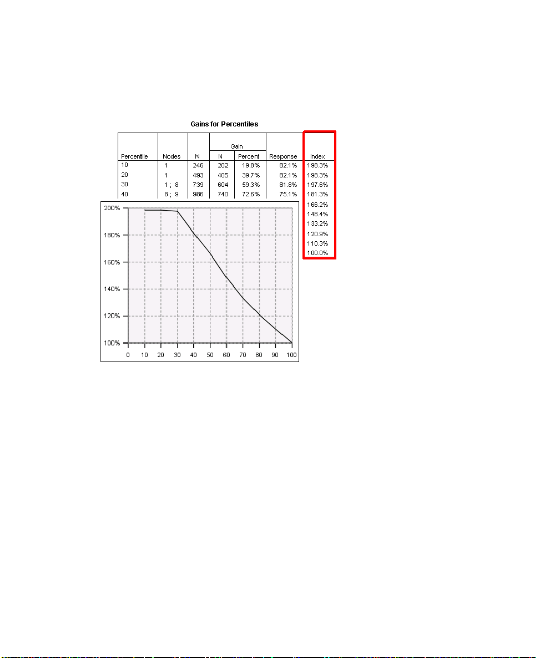
Index is the ratio of the node response percentage for the target category

Index.

compared to the overall target category response percentage for the entire sample.
The index chart is a line chart of cumulative percentile index values. Available only

egorical dependent variables. Cumulative percentile index is computed as:

for cat
(cumulative percentile response percent / total response percent) x 100. A separate
chart is produced for each target category, and target categories must be d efined.

The index chart plots the same values that you would see in the Index column in

ins for percentiles table.

the ga

42

Chapter 1

Figure 1-28

Gains for percentiles table and index chart

Mean. Line chart of cumulative percentile mean values for the dependent variable.

Available only for scale dependent variables.

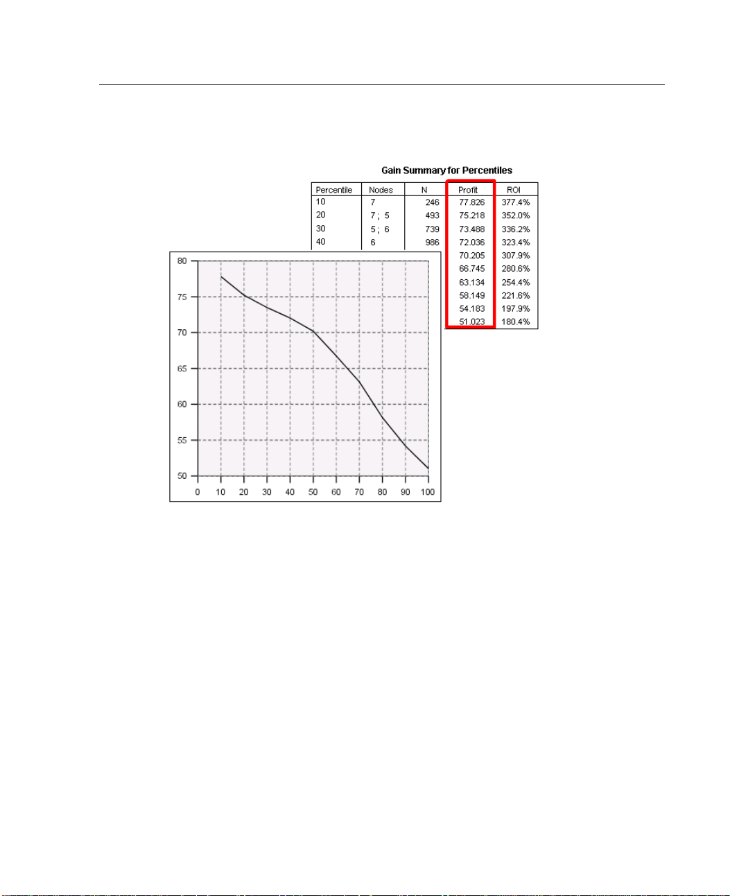
Average profit. Line chart of cumulative average profit. Available only for categorical

dependent variables with defined profits. For more information, see “Profits” on p. 21.

The average profit chart plots the same values that you would see in the Profit column
in the gain summary for percentiles table.

43

Figure 1-29

Gain summary for percentiles table and average profit chart

Creating Class

ification Trees

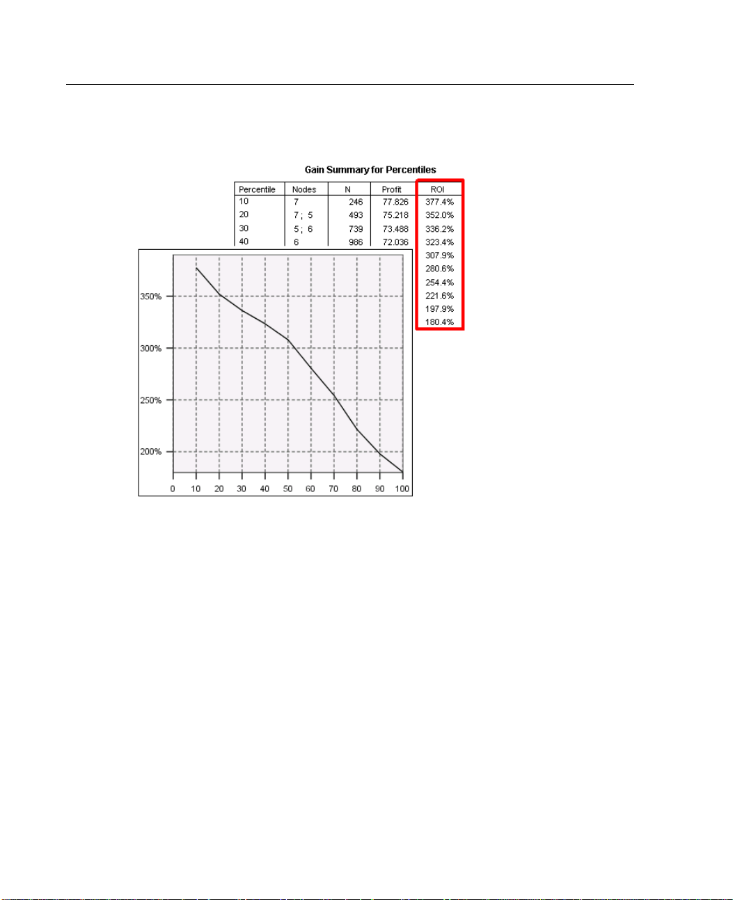
Return on investment (ROI). Line chart of cumulative ROI (return on investment).

ROI is computed as the ratio of profits to expenses. Available only for categorical
dependent variables with defined profits.

The ROI chart plots the same values that you would see in the ROI column in the gain
summary for percentiles table.

44

Chapter 1

Figure 1-30

Gain summary for percentiles table and ROI chart

Percentile increment. For all percentile charts, this setting controls the percentile

increments displayed on the chart: 1, 2, 5, 10, 20, or 25.

45

Selection and Scoring Rules

Figure 1-31

Output dialo

gbox,Rulestab

Creating Class

ification Trees

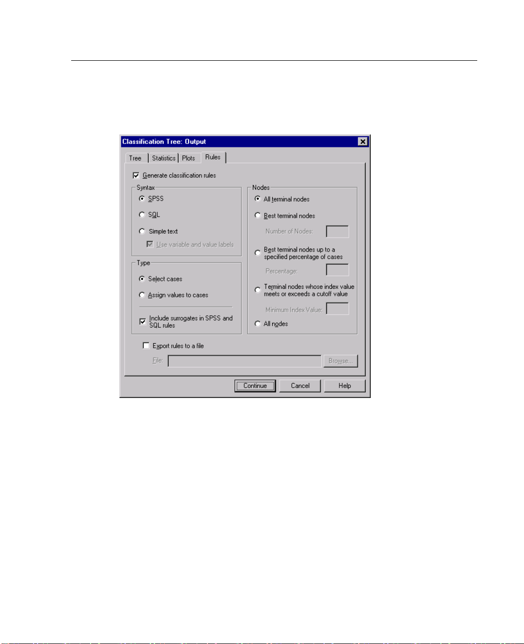
The Ru

les tab provides the ability to generate selection or classification/prediction
rules in the form of SPSS command syntax, SQL, or simple (plain English) text. You
can display these rules in the Viewer and/or save the rules to an external file.

Syntax. Controls the form of the selection rules in both output displayed in the Viewer

lectionrulessavedtoanexternalfile.

and se

.

 SPSS

SPSS command language. Rules are expressed as a set of commands that

define a filter condition that can be used to select subsets of cases or as

COMPUTE

statements that can be used to score cases.

46

Chapter 1



SQL. Standard SQL rules are generated to select or extract records from a database

or assign va

lues to those records. The generated SQL rules do not include any

table names or other data source information.

 Simple text. Plain English pseudo-code. Rules are expressed as a set of logical

“if...then” statements that describe the model’s classifications or predictions
for each nod

e. Rules in this form can use defined variable and value labels or

variable names and data values.

Type. For SPSS and SQL rules, controls the type of rules generated: selection or

scoring ru

 Select ca

les.

ses.

The rules can be used to select cases that meet node membership
criteria. For SPSS and SQL rules, a single rule is generated to select all cases that
meet the selection criteria.

 Assign values to cases. The rules can be used to assign the model’s predictions

to cases th

at meet node membership criteria. A separate rule is generated for

each node that meets the node membership criteria.

Include s

urrogates in SPSS and SQL rules.

For CRT and QUEST, you can include
surrogate predictors from the model in the rules. Rules that include surrogates can be
quite complex. In general, if you just want to derive conceptual information about
your tree

, exclude surrogates. If some cases have incomplete independent variable
(predictor) data and you want rules that mimic your tree, include surrogates. For more
information, see “Surrogates” on p. 18.

Nodes. Controls the scope of the generated rules. A separate rule is generated for

each nod

 All ter

 Best te

e included in the scope.

minal nodes.

rminal nodes.

Generates rules for each terminal node.

Generates rules for the top n terminal nodes based on index
values. If the number exceeds the number of terminal nodes in the tree, rules are
generated for all terminal nodes. (See note below.)

 Best terminal nodes up to a specified percentage of cases. Generates rules for

al nodes for the top n percentage of cases based on index values. (See

termin
note below.)

 Terminal nodes whose index value meets or exceeds a cutoff value. Generates rules

for all terminal nodes with an index value greater than or equal to the specified

An index value greater than 100 means that the percentage of cases in

value.

47

Creating Class

ification Trees

the target category in that node exceeds the percentage in the root node. (See
note below.

 All nodes. G

)

enerates rules for all nodes.

Note 1: Node selection based on index values is available only for categorical
dependent variables with defined target categories. If you have specified multiple
target cate

gories, a separate set of rules is generated for each target category.

Note 2: For SPSS and SQL rules for selecting cases (not rules for assigning values),

All nodes and All terminal nodes will effectively generate a rule that selects all cases

used in the a

Export rule

You can als

nalysis.

s to a file.

Saves the rules in an external text file.

o generate and save selection or scoring rules interactively, based on
selected nodes in the final tree model. For more information, see “Case Selection and
Scoring Rules” in Chapter 2 on p. 58.

Note:Ifyo

u apply rules in the form of SPSS command syntax to another data file,
that data file must contain variables with the same names as the independent variables
included in the final model, measured in the same metric, with the same user-defined
missing v

alues (if any).

Tree Editor

With the Tree Editor, you can:

 Hide and show selected tree branches.
 Control display of node content, statistics displayed at node splits, and other

information.

 Change node, background, border, chart, and font colors.
 Change font style and size.
 Change tree alignment.
 Select subsets of cases for further analysis based on selected nodes.
 Create and save rules for selecting or scoring cases based on selected nodes.

Chapter

2

To edit a tree model:

E Double-click the tree model in the Viewer window.

or

E Right-cli

SPSS Tree Object

Open

Hiding and S

To hide (col

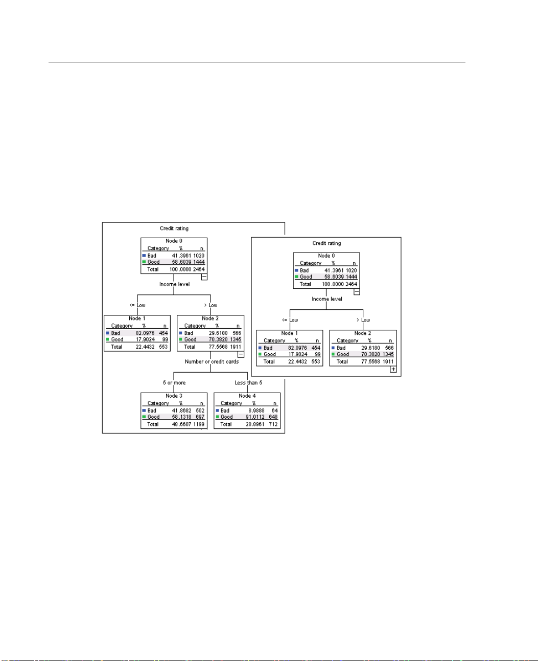
E Click the m

node.

All nodes beneath the parent node on that branch will be hidden.

ck the tree model in the Viewer window, and from the context menu choose:

howing Nodes

lapse) all the child nodes in a branch beneath a parent node:

inus sign (–) in the small box below the lower right corner of the parent

49

50

Chapter 2

To show (expand) the child nodes in a branch beneath a parent node:

E Click the plus sign (+) in the small box below the lower right corner of the parent node.

Note: Hiding the child n odes on a branch is not the same as pruning a tree. If you
want a pruned

tree, you must request pruning before you create the tree, and pruned
branches are not included in the final tree. For more information, see “Pruning
Trees” in Chapter 1 on p. 17.

Figure 2-1

Expanded and collapsed tree

Selecting Multiple Nodes

You can select cases, generate scoring and selections rules, and perform other actions
based on the currently selected node(s). To select multiple nodes:

E Click a node you want to select.
E Ctrl-click the other nodes you want to select.

You can multiple-select sibling nodes and/or parent nodes in one branch and child
nodes in another branch. You cannot, however, use multiple selection on a parent
node and a ch

ild/descendant of the same node branch.

Working with Large Trees

Treemodelsmaysometimescontainsomanynodesandbranchesthatitisdifficultor
impossibl
you may find useful when working with large trees:

 Tree map. You can use the tree map, a much smaller, simplified version of the

 Scaling. You can zoom out and zoom in by changing the scale percentage for the

 Node and branch display. You can make a tree more compact by displaying only

e to view the entire tree at full size. There are a number of features that

tree, to na

vigate the tree and select nodes. For more information, see “Tree

Map” on p. 51.

tree display. For more information, see “Scaling the Tree Display” on p. 52.

tables or o

nly charts in the nodes and/or suppressing the display of node labels
or independent variable information. For more information, see “Controlling
Information Displayed in the Tree” on p. 55.

51

Tre e Ed i t or

Tree Map

E From the Tree Editor menus choose:

Thetreem

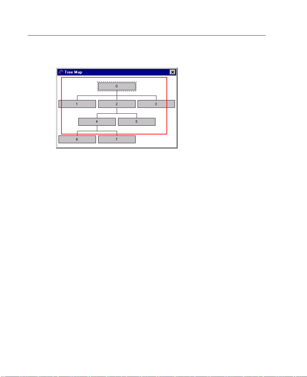
ap provides a compact, simplified view of the tree that you can use to

navigate the tree and select nodes.

To use the tree map window:

View

Tree Map

52

Chapter 2

Figure 2-2

Tree map window

 The currently selected node is highlighted in both the Tree Model Editor and

thetreemapwindow.

 The portion of the tree that is currently in the Tree Model Editor view area is

indicate

d with a red rectangle in the tree map. Right-click and drag the rectangle

to change the section of the tree displayed in the view area.

 If you select a node in the tree map that isn’t currently in the Tree Editor view

area, the view shifts to include the selected node.

 Multiple node selection works the same in the tree map as in the Tree Editor:

ick to select multiple nodes. You cannot use multiple selection on a parent

Ctrl-cl
node and a child/descendant of the same node branch.

Scaling the Tree Display

By default, trees are automatically scaled to fit in the Viewer window, which can
result in some trees that are initially very difficult to read. You can select a preset

etting or enter your own custom scale value of between 5% and 200%.

scale s

Tre e Ed i t or

To change the scale of the tree:

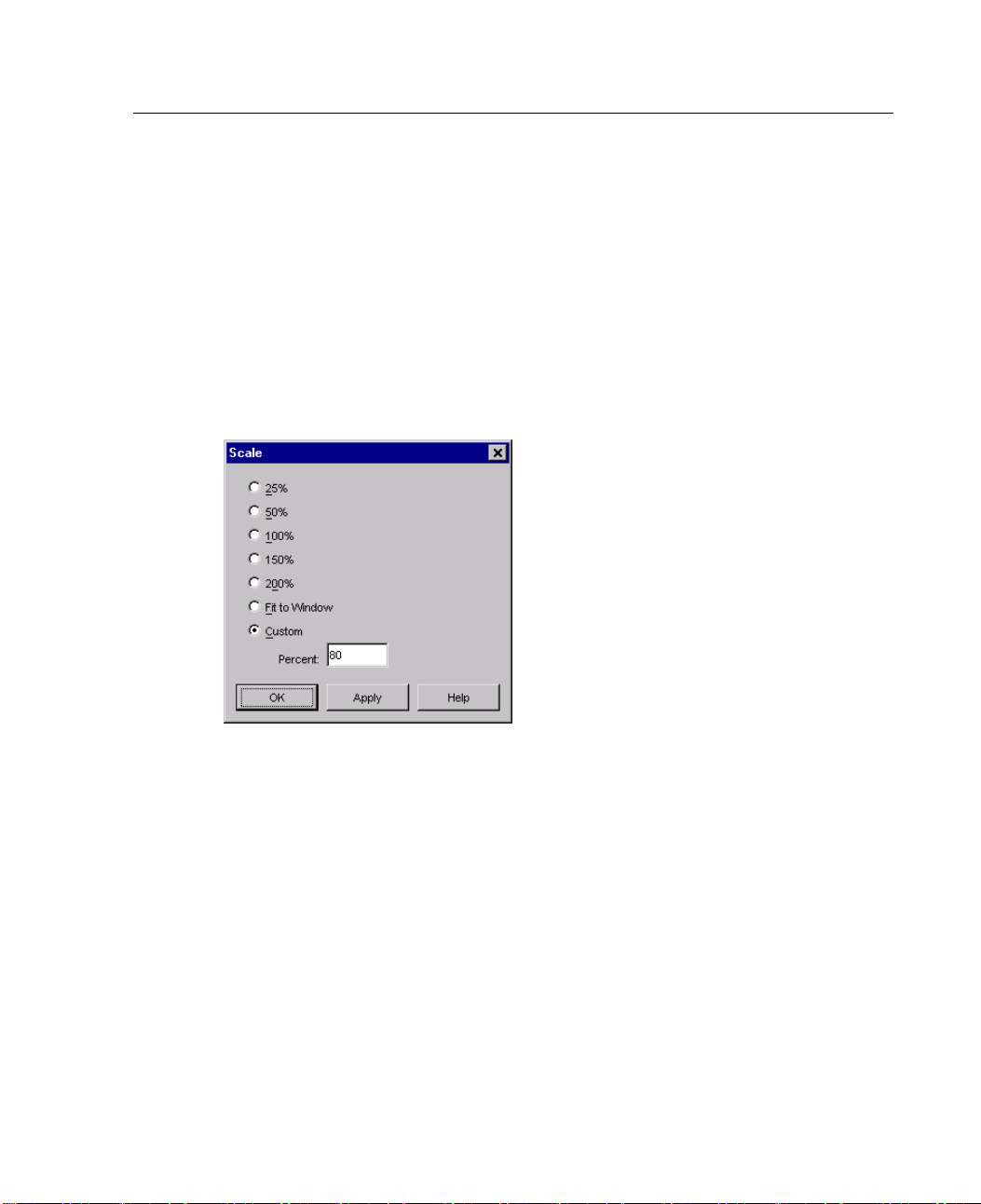
E Select a scale percentage from the drop-down list on the toolbar, or enter a custom

percentage value.

or

E From the Tree Editor menus choose:

View

Scale...

Figure 2-3

Scaledialogbox

53

You can also specify a scale value before you create the tree model. For more
information, see “Output” in Chapter 1 on p. 30.

Node Summary Window

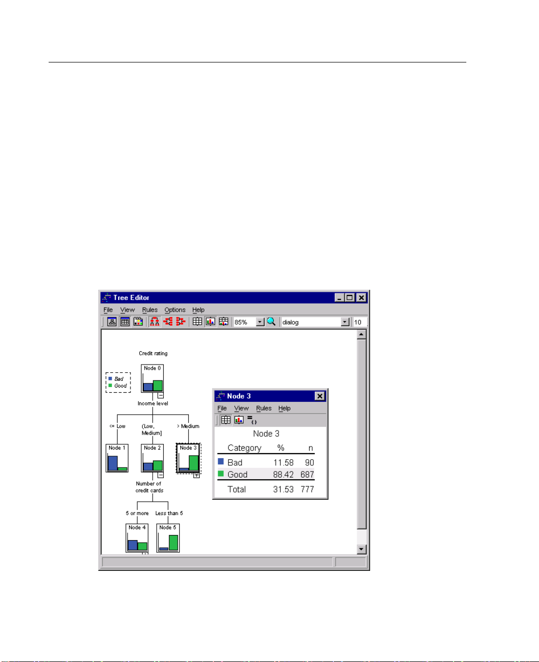
The node summary window provides a larger view of the selected nodes. You can
also use the summary window to view, apply, or save selection or scoring rules
based on the selected nodes.

 Use the View menu in the node summary window to switch between views

of a summary table, chart, or rules.

54

Chapter 2



Use the Rules menu in the node summary window to select the type of rules you

want to see.

For more information, see “Case Selection and Scoring Rules” on

p. 58.

 All views in the node summary window reflect a combined summary for all

selected nodes.

To use the node summary window:

E Select the nodes in the Tree Editor. To select multiple nodes, use Ctrl-click.
E From the menus choose:

View

Summary

Figure 2-4

Tree with charts in nodes and table for selected node in summary window

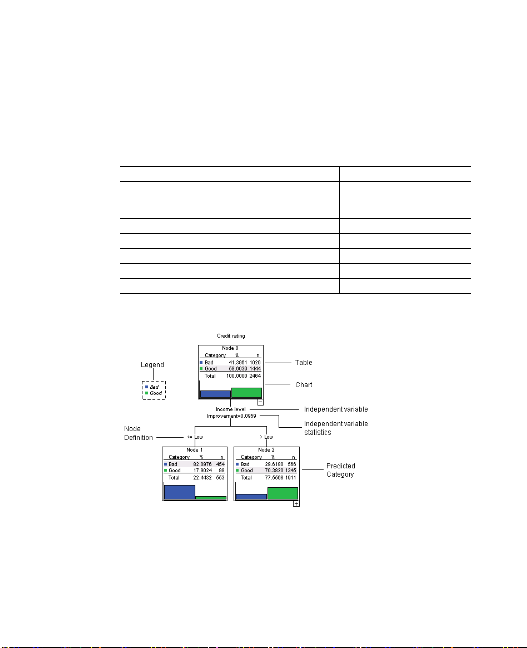
55

Tre e Ed i t or

Controlling

The Options
contents, independent variable (predictor) names and statistics, node definitions, and
other settings. Many of these settings can be also be controlled from the toolbar.

Setting Options Men

Highlight predicted category (categorical dependent
variable)

Tables and/or charts in node Node Contents
Significance test values and p values Independent Variable Statistics
Independent (predictor) variable names Independent Variables
Independent (predictor) value(s) for node s Node Definitions
Alignment (top-down, left-right, right-left) Orientation
Chart legend Legend

Figure 2-5

Tree elements

Information Displayed in the Tree

menu in the Tree Editor allows you to control the display of node

u Selection

Highlight Predicted

56

Chapter 2

Changing Tre

You can chan

 Node border
 Branch colo
 Tree backgr
 Predicted c
 Node chart c

You can also c
Note: You cannot change color or font attributes for individual nodes or branches.

Color changes apply to all elements of the same type, and font changes (other than
color) appl

To change co

E Use the too

elements. (ToolTips describe each control on the toolbar when you put the mouse
cursor on the control.)

or

e Colors and Text Fonts

ge the following colors in the tree:

, background, and text color
r and branch text color
ound color

ategory highlight color (categorical dependent variables)

olors

hange the type font, style, and size for all text in the tree.

ytoallchartelements.

lors and text font attributes:

lbar to change font attributes for the entire tree or colors for different tree

E Double-click anywhere in the Tree Editor to open the Properties window, or from

the menus choose:

View

Propertie

For borde

E

the

E For font colors and attributes, click the Text tab.
E For node chart colors, click the Node Charts tab.

s

r, branch, node background, predicted category, and tree background, click

Color tab.

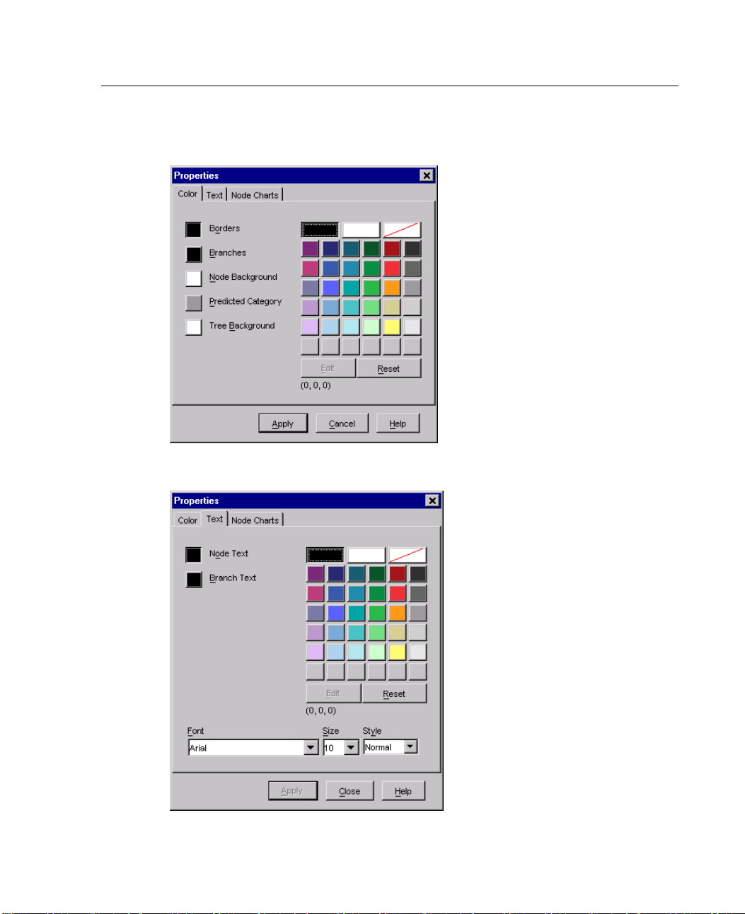
Figure 2-6

Properties window, Color tab

Figure 2-7

Properties window, Text tab

57

Tre e Ed i t or

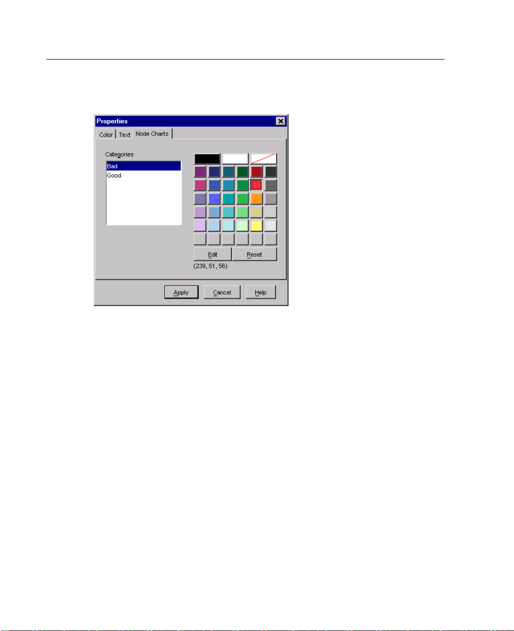
58

Chapter 2

Figure 2-8

Properties window, Node Charts tab

Case Selection and Scoring Rules

You can use the Tree Editor to:

 Select subsets of cases based on the selected node(s). For more information, see

“Filtering Cases” on p. 58.

 Generate case selection rules or scoring rules in SPSS or SQL format. For more

ation, see “Saving Selection and Scoring Rules” on p. 59.

inform

You can also automatically save rules based on various criteria when you run the
Classification Tree procedure to create the tree model. For more information, see

tion and Scoring Rules” in Chapter 1 on p. 45.

“Selec

Filtering Cases

If you want to know more about the cases in a particular node or group of nodes, you

ect a subset of cases for further analysis based on the selected nodes.

can sel

E Sele

ct the nodes in the Tree Editor. To select multiple nodes, use Ctrl-click.

E

From the menus choose:

Rules

Filter Cases...

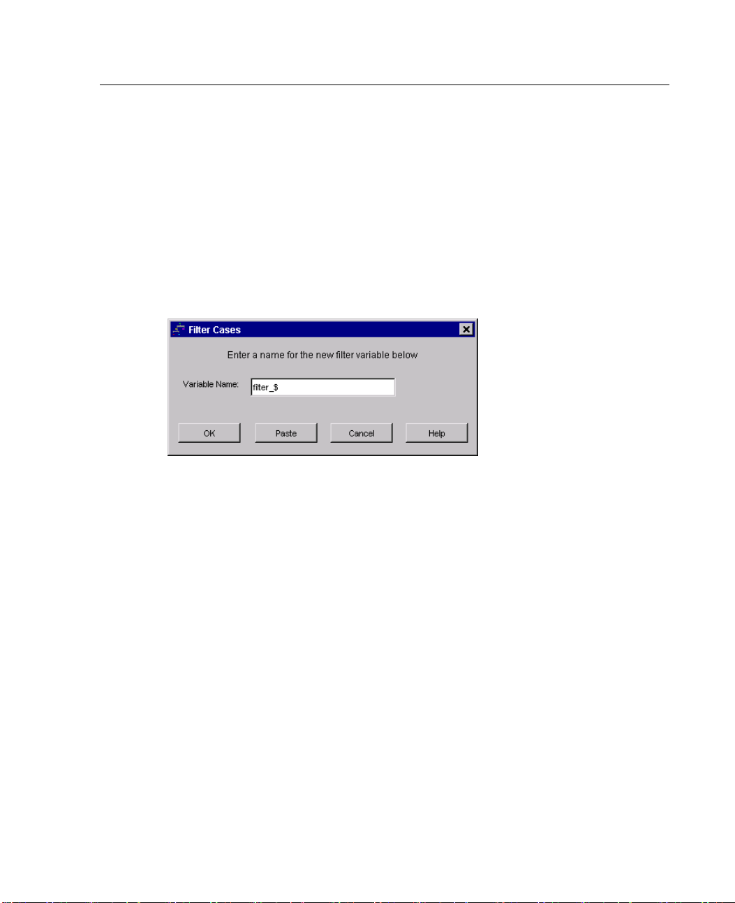
Enter a filter variable name. Cases from the selected nodes will receive a value of 1

E

for this vari

able. All other cases will receive a value of 0 and will be excluded from

subsequent analysis until you change the filter status.

E Click OK.

59

Tre e Ed i t or

Saving Se

Figure 2-9

Filter Case

s dialog box

lection and Scoring Rules

You can sa
rules to a different data source. The rules are based on the selected nodes in the
Tree Editor.

Syntax.

andselectionrulessavedtoanexternalfile.

 SPSS. SPSS command language. Rules are expressed as a set of commands that

 SQL. Standard SQL rules are generated to select/extract records from a database

ve case selection or scoring rules in an external file and then apply those

Controls the form of the selection rules in both output displayed in the Viewer

define a

filter condition that can be used to select subsets of cases or as

COMPUTE

statements that can be used to score cases.

or assign values to those records. The generated SQL rules do not include any

ames or other data source information.

table n

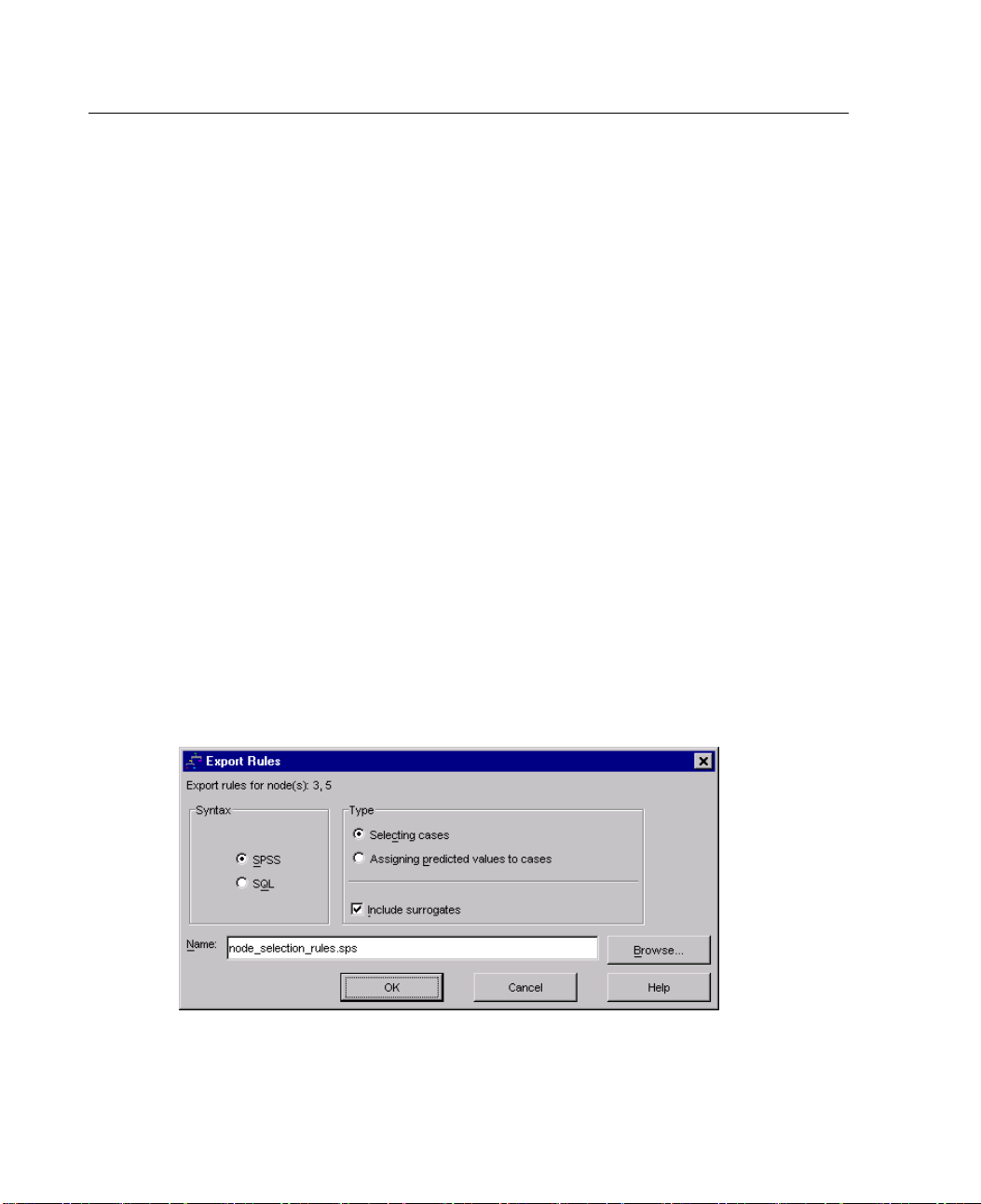
Type. You can create selection or scoring rules.

60

Chapter 2



Select cases. The rules can be used to select cases that meet node membership

criteria. F

or SPSS and SQL rules, a single rule is generated to select all cases that

meet the selection criteria.

 Assign values to cases. The rules can be used to assign the model’s predictions

to cases that meet node membership criteria. A separate rule is generated for
each node th

at meets the node membership criteria.

Include surrogates. For CRT and QUEST, you can include surrogate predictors from

the model in the rules. Rules that include surrogates can be quite complex. In
general, i

f you just want to derive conceptual information about your tree, exclude
surrogates. If some cases have incomplete independent variable (predictor) data and
you want rules that mimic your tree, include surrogates. For more information,
see “Surro

gates” in Chapter 1 on p. 18.

To save ca

E Select t
E From the

Rules

Export...

Select the type of rules you want and enter a filename.

E

Figure 2-

Export Ru

se selection or scoring rules:

he nodes in the Tree Editor. To select multiple nodes, use Ctrl-click.

menus choose:

10

les dialog box

61

Tre e Ed i t or

Note: If you apply rules in the form of SPSS command syntax to another data file,
that data file must contain variables with the same names as the independent variables
included in

the final model, measured in the same metric, with the same user-defined

missing values (if any).

Chapter

3

Data Assumpt

ions and

Requirements

The Classification Tree procedure assumes that:

 The appropriate measurement level has been assigned to all analysis variables.
 For categorical (nominal, ordinal) dependent variables, value labels have been

defined for all categories that should be included in the analysis.

We’ll use the file tree_textdata.sav to illustrate the importance of both of these
requirements. This data file reflects the default state of data read or entered into SPSS
before defining any attributes, such as measurement level or value labels. This file is
located in the tutorial\sample_files directory of the SPSS installation directory.

Effects of Measurement Level on Tree Models

Both variables in this data file are numeric. By default, numeric variables are assumed
to have a scale measurement level. But (as we will see later) both variables are really
categorical variables that rely on numeric codes to stand for category values.

E To run a Classification Tree analysis, from the menus choose:

Analyze

Classify

Tree...

63

64

Chapter 3

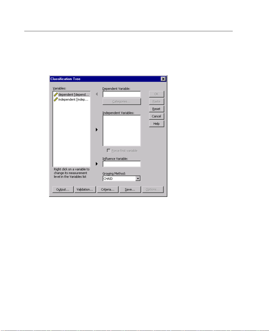
The icons next to the two variables in the source variable list indicate that they will
be treated as scale variables.

Figure 3-1

Classification Tree main dialog box with two scale variables

E Select dependent as the dependent variable.
E Select independent as the independent variable.
E Click OK to run the procedure.
E Open the Classification Tree dialog box a gain and click Reset.
E Right-click dependent inthesourcelistandselectNominal from the context menu.
E Dothesameforthevariableindependent in the source list.

65

Data Assumptio

ns and Requiremen ts

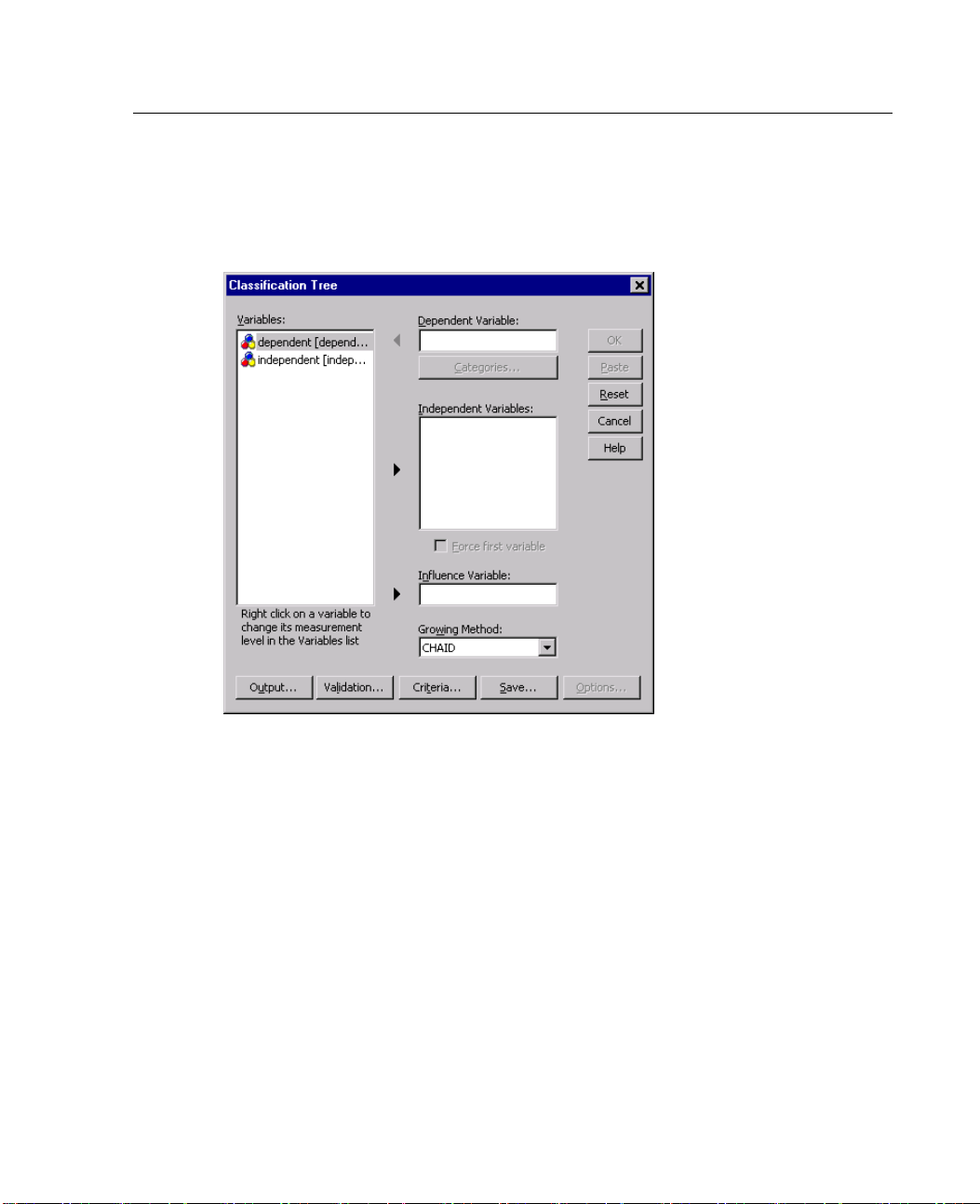
Now the icons next to each variable indicate that they will be treated as nominal
variables.

Figure 3-2

Nominal icons in source list

E Select dependent as the dependent variable and independent as the independent

variable, and click OK to run the procedure again.

66

Chapter 3

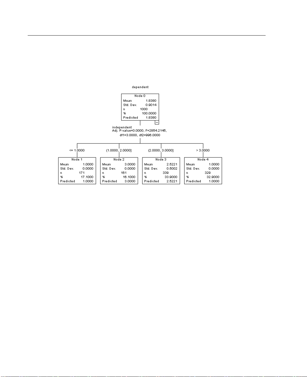
Now let’s compare the two trees. First, we’ll look at the tree in which both numeric
variables are treated as scale variables.

Figure 3-3

Tree with both variables treated as scale

 Each node of tree shows the “predicted” value, which is the mean value for the

dependent variable at that node. For a variable that is actually categorical, the
mean may not be a meaningful statistic.

 The tree has four child nodes, one for each value of the independent variable.

Tree models will often merge similar nodes, but for a scale variable, only contiguous
values can be merged. In this example, no contiguous values were considered similar
enough to merge any nodes together.

67

Data Assumptio

ns and Requiremen ts

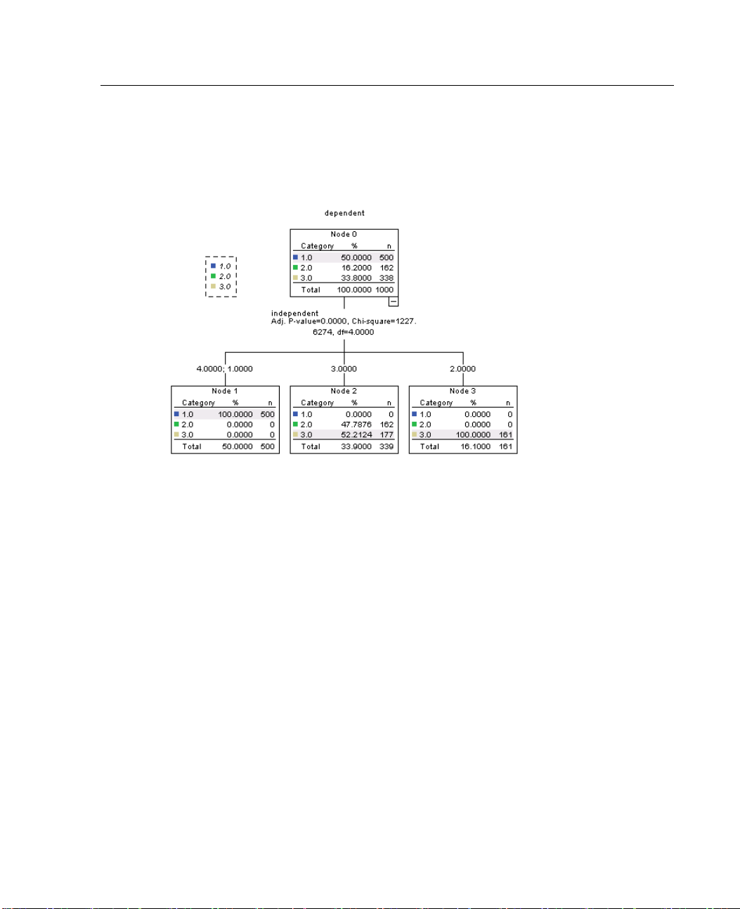
The tree in which both variables are treated as nominal is somewhat different in

several respects.

Figure 3-4

Tree with both variables treated as nominal

 Instead of a predicted value, each node contains a frequency table that shows the

number of cases (count and percentage) for each category of the dependent
variable.

 The “predicted” category—the category with the highest count in each node—is

highlighted. For example, the predicted category for node 2 is category 3.

 Instead of four child nodes, there are only three, with two values of the

independent variable merged into a single node.

The two independent values merged into the same node are 1 and 4. Since, by
definition, there is no inherent order to nominal values, merging of noncontiguous
values is allowed.

Permanently Assigning Measurement Level

When you change the measurement level for a variable in the Classification
Tree dialog box, the change is only temporary; it is not saved with the data file.
Furthermore, you may not always know what the correct measurement level should
be for all variables.

68

Chapter 3

Define Variable Properties can help you determine the correct measurement level
for each variable and permanently change the assigned measurement level. To use
Define Vari

able Properties:

E From the me

Data

Define Variable Properties...

Effects of V

The Classif
of a categorical (nominal, ordinal) dependent variable have defined value labels or
none of them do. Some features are not available unless at least two nonmissing
values of t
nonmissing values have defined value labels, any cases with other values that do not
have value labels will be excluded from the analysis.

The origin
the dependent variable is treated as nominal, the tree model uses all nonmissing
values in the analysis. In this example, those values are 1, 2, and 3.

But what ha
the dependent variable?

E In the Data Editor window, click the Variable View tab.
E Click the Values cell for the variable dependent.

nus choose:

alue Labels on Tree Models

ication Tree dialog box interface assumes that either all nonmissing values

he categorical dependent variable have value labels. If at least two

al data file in this example contains no defined value labels, and when

ppens when we define value labels for some, but not all, values of

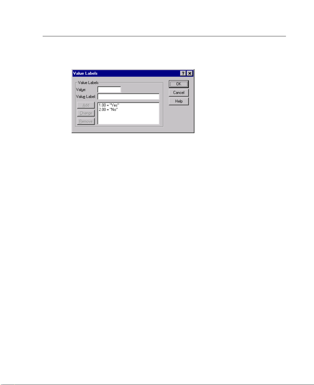
69

Data Assumptio

Figure 3-5

Defining value labels for dependent variable

E First, enter 1 for Value and Yes for Value Label, and t hen click Add.
E Next, enter 2 for Value and No for Value Label, and then click Add again.
E Then click OK.
E Open the Classification Tree dialog box again. The dialog box should still have

ns and Requiremen ts

dependent selected as the dependent variable, with a nominal measurement level.

E Click OK to run the procedure again.

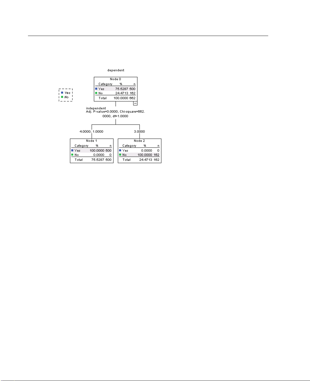
70

Chapter 3

Figure 3-6

Tree for nominal dependent variable with partial value labels

Now only the two dependent variable values with defined value labels are included
in the tr

ee model. All cases with a value of 3 for the dependent variable have been

excluded, which might not be readily apparent if you aren’t familiar with the data.

Assigni

ng Value Labels to All Values

To avoid
Variable Properties to assign value labels to all dependent variable values found
in the data.

accidental omission of valid categorical values from the analysis, use Define

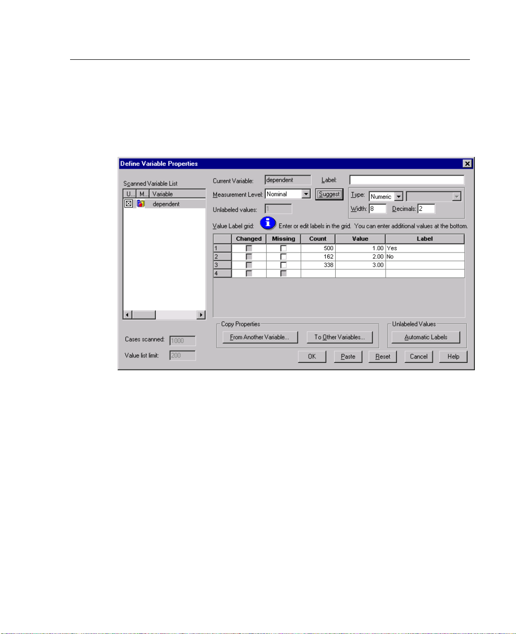
71

Data Assumptio

ns and Requiremen ts

When the data dictionary information for the variable name isdisplayedintheDefine
Variable Properties dialog box, you can see that although there are over 300 cases
with a value

Figure 3-7

Variable with partial value labels in Define Variable Properties dialog box

of 3 for that variable, no value label has been defined for that value.

Chapter

4

Using Classi

fication Trees to

Evaluate Credit Risk

Abankmain
out loans from the bank, including whether or not they repaid the loans or defaulted.
Using classification trees, you can analyze the characteristics of the two groups
of custome
default on their loans.

Thecreditdataarestoredintree_credit.sav,locatedinthetutorial\sample_files

director

Creating t he Model

The Classification Tree Procedure offers several different methods for creating tree
models. F

tains a database of historic informationoncustomerswhohavetaken

rs and build models to predict the likelihood that loan applicants will

y of the SPSS installation directory.

or this example, we’ll use the default method:

Buildin

CHAID. Chi-squared Automatic Interaction Detection. At each step, CHAID

chooses the independent (predictor) variable that has the strongest interaction with
the depe
significantly different with respect to the dependent variable.

g the CHAID Tree Model

E To run a

Analyze

ndent variable. Categories of each predictor are merged if they are not

Classification Tree analysis, from the menus choose:

Classify

Tree...

73

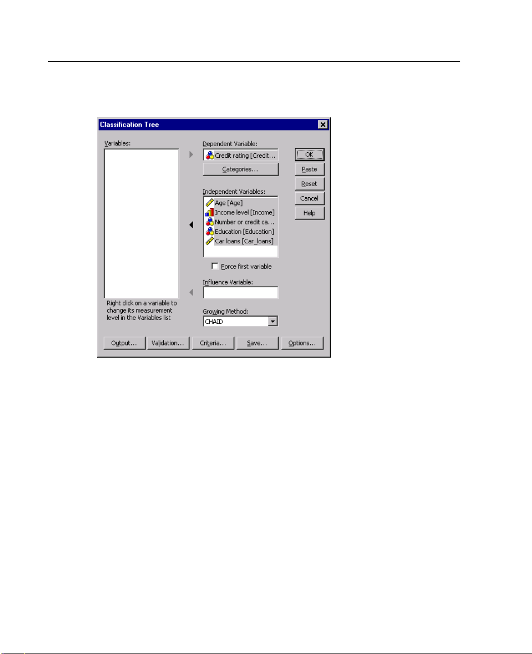
74

Chapter 4

Figure 4-1

Classification Tree dialog box

E Select Credit rating as the dependent variable.
E Select all the remaining variables as independent variables. (The procedure will

automatically exclude any variables that don’t make a significant contribution to

al model.)

the fin
At this point, you could run the procedure and produce a basic tree model, but we’re

going to select some additional output and make a few minor adjustments to the

ia used to generate the model.

criter

Selecting Target Categories

E Click the Categories button right below the selected dependent variable.

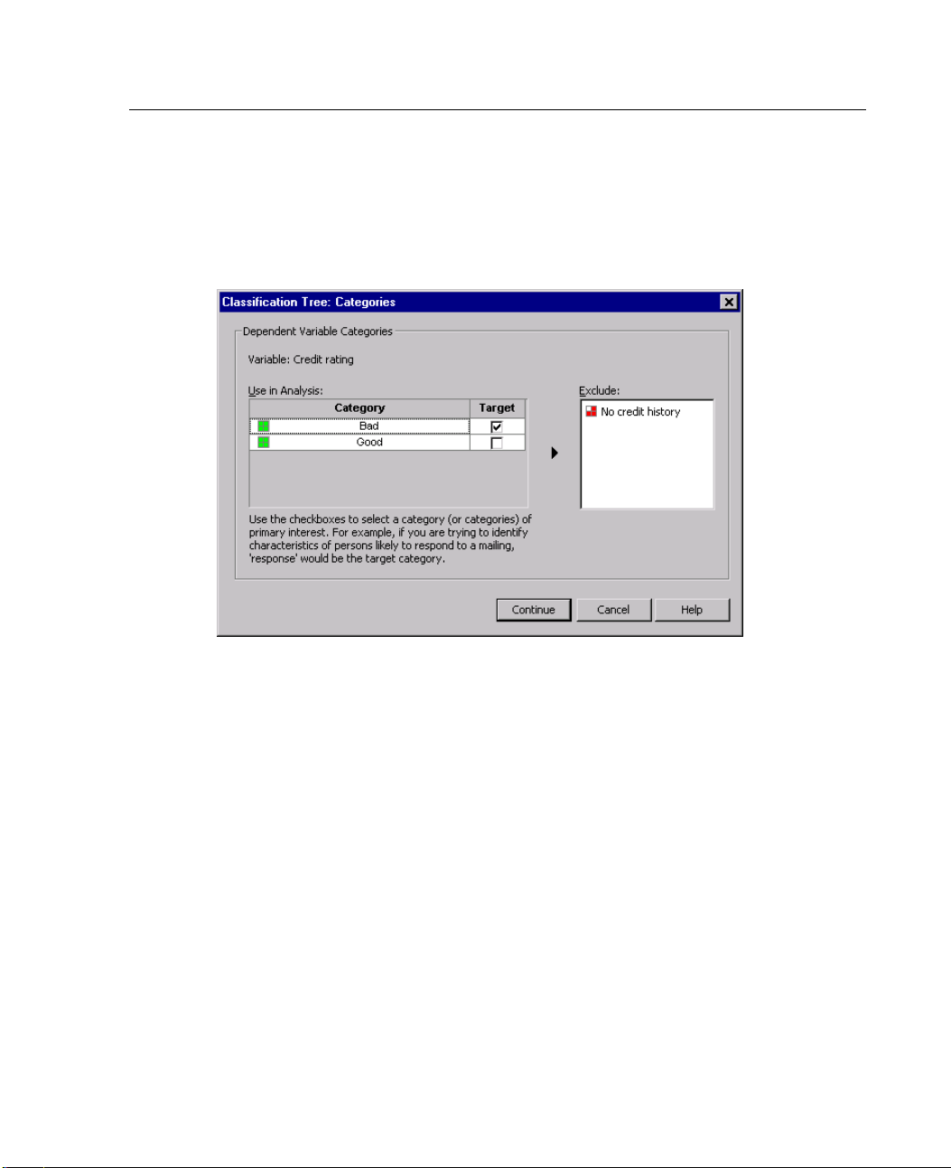
75

Using Classifi

cation Trees to Evaluate Credit Risk

This opens the Categories dialog box, where you can specify the dependent variable
target categories of interest. Target categories do not affect the tree model itself, but
some output

Figure 4-2

Categories dialog box

and options are available only if you have selected target categories.

E Select (check) the Target check box for the Bad category. Customers with a bad credit

(defaulted on a loan) will be treated as the target category of interest.

rating

.

E Click C

ontinue

Specifying Tree Growing Criteria

For t his example, we want to keep the tree fairly simple, so we’ll limit the tree growth

ing the minimum number of cases for parent and child nodes.

by rais

E In the m

ain Classification Tree dialog box, click

Criteria.

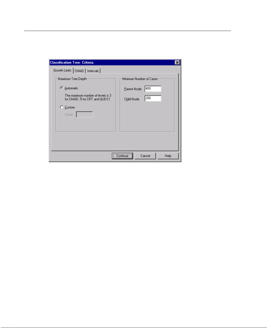
76

Chapter 4

Figure 4-3

Criteria dialog box, Growth Limits tab

E In the Minimum Number of Cases group, type 400 for Parent Node and 200 for

Child N

ode.

.

E Click C

ontinue

Selecting Additional Output

E In the main Classification Tree dialog box, click Output.

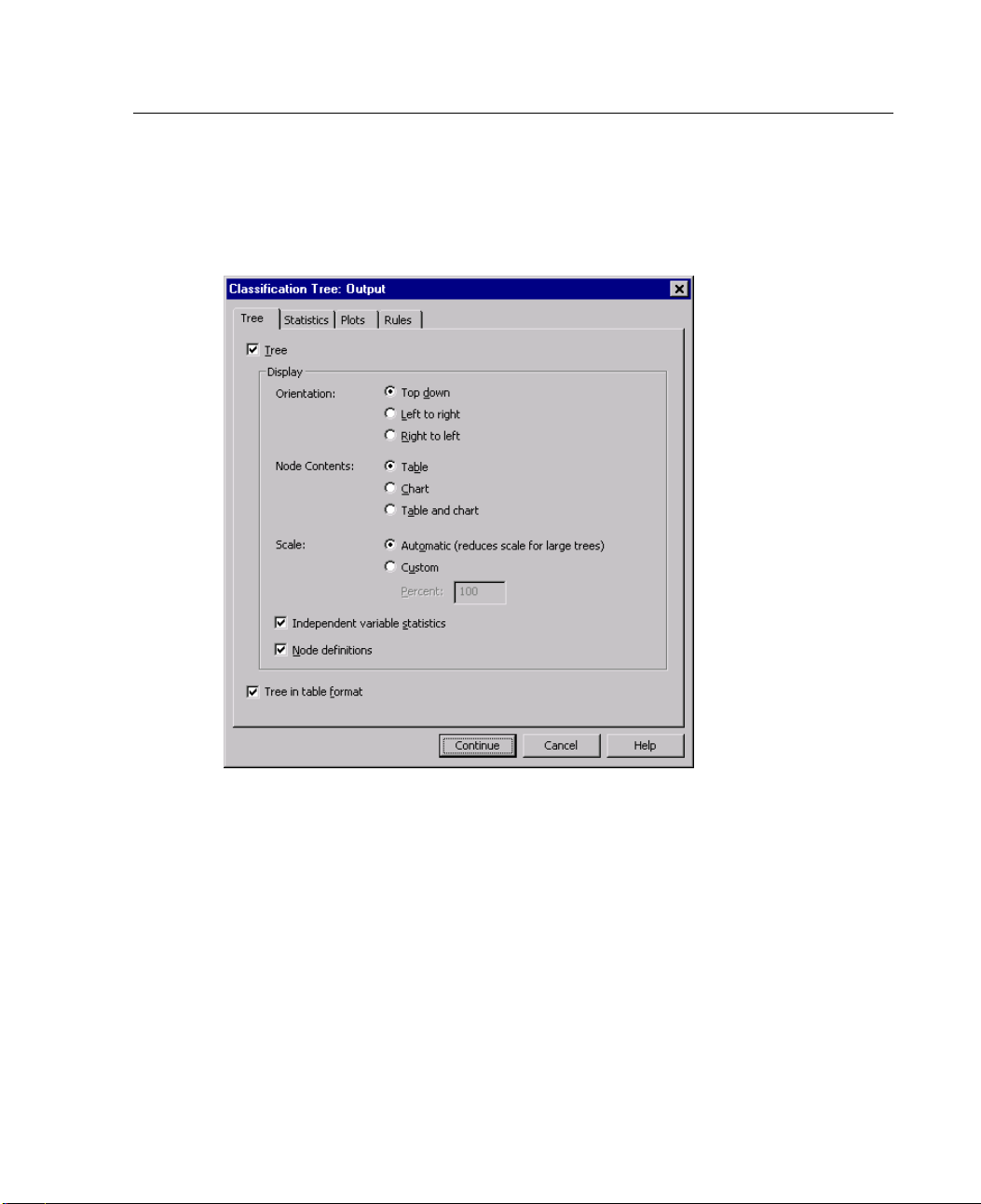
77

Using Classifi

cation Trees to Evaluate Credit Risk

This opens a tabbed dialog box, where you can select various types of additional
output.

Figure 4-4

Output dialog box, Tree t ab

E On the Tree tab, select (check) Tree in table format.
E Then click the Plots tab.

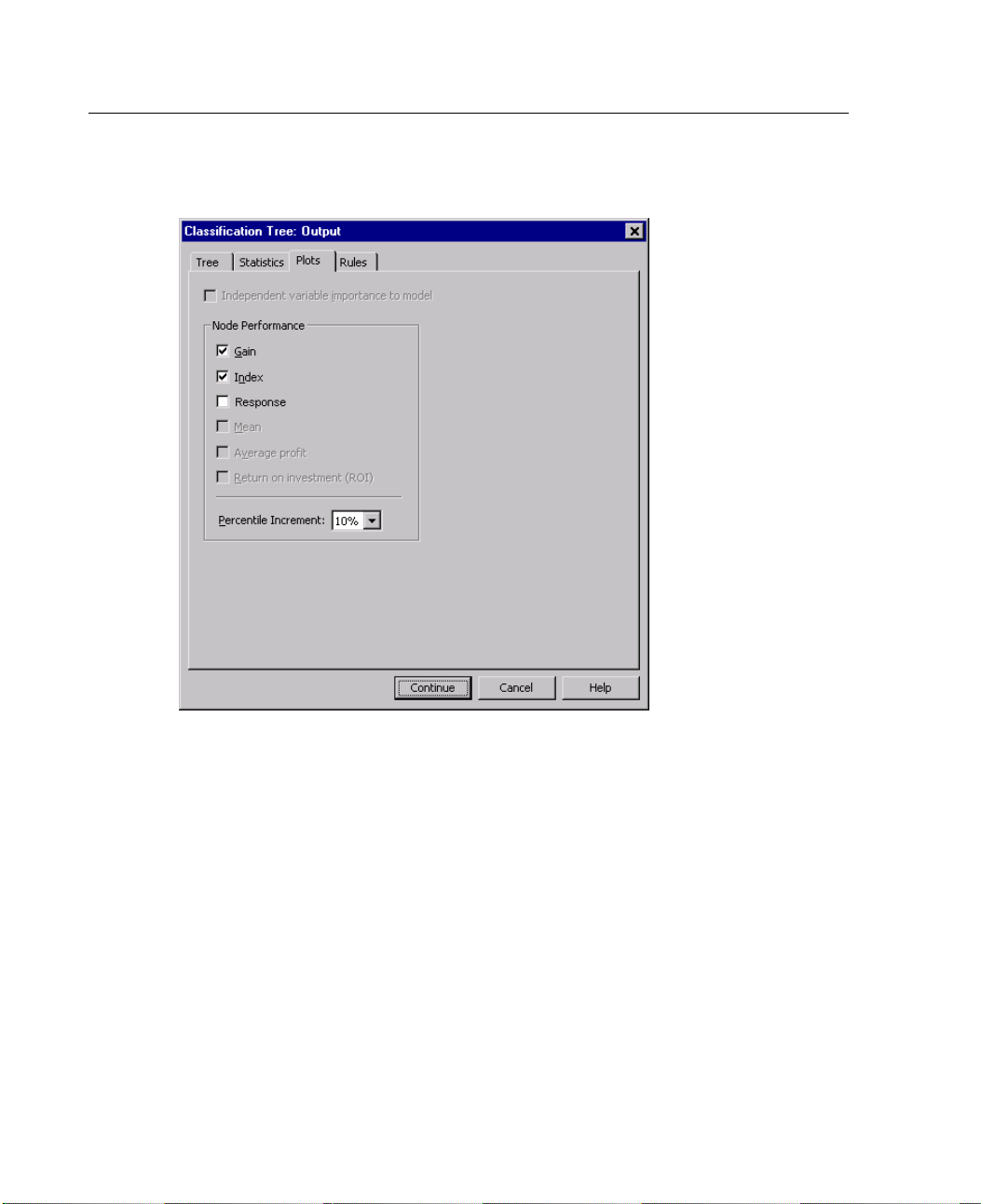
78

Chapter 4

Figure 4-5

Output dialog box, Plots tab

Saving

E Select (check) Gain and Index.

Note: These charts require a target category for the dependent variable. In this
exampl

e, the Plots tab isn’t accessible until after you have specified one or more

target categories.

E Click Continue.

Predicted Values

You can
example, you can save the credit rating predicted for each case and then compare
those predictions to the actual credit ratings.

save variables that contain information about model predictions. For

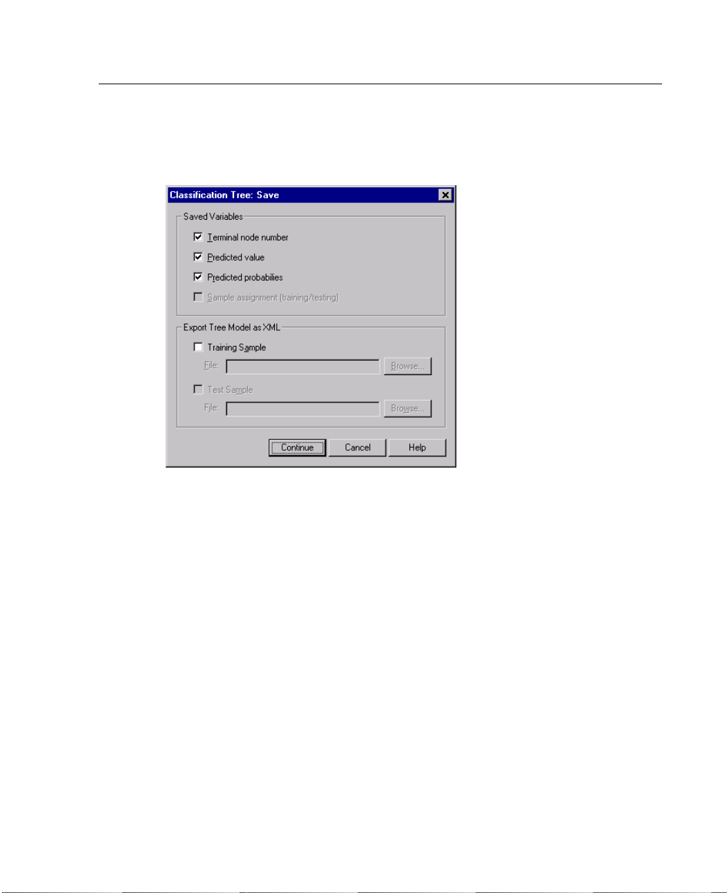
79

Using Classifi

E

In the main Classification Tree dialog box, click Save.

Figure 4-6

Save dialog b

E Select

(check)

ox

Terminal node number, Predicted value,andPredicted probabilities.

cation Trees to Evaluate Credit Risk

.

E Click C
E In the ma

ontinue

in Classification Tree dialog box, click

Evaluating the Model

For this example, the model results include:

 Tables that provide information about the model.
 Tree diagram.
 Charts that provide an indication of model performance.
 Model prediction variables added to the working data file.

OK to run the procedure.

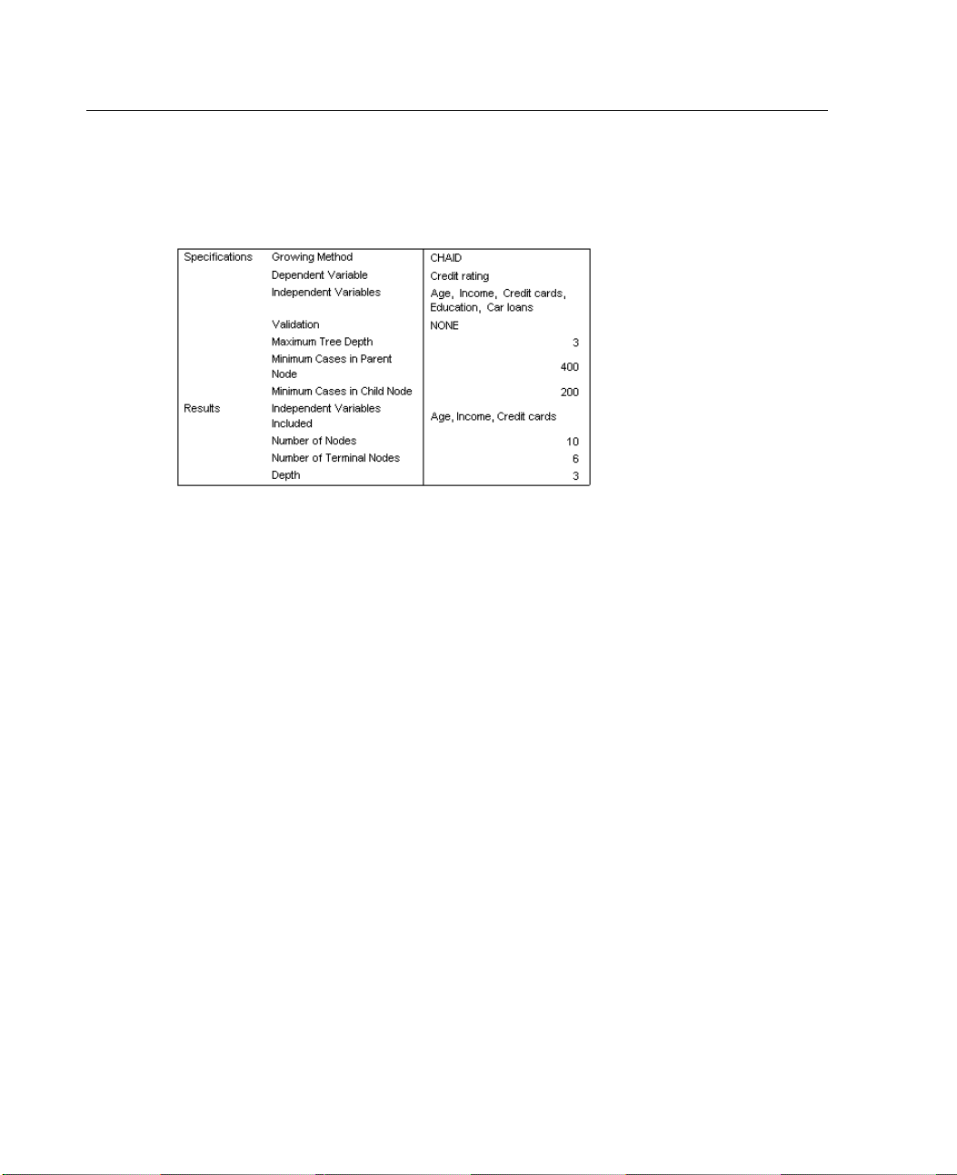
80

Chapter 4

Model Summary Table

Figure 4-7

Model summar

y

The model summary table provides some very broad information about the
specific

 The Spec

ations used to build the model and the resulting model.

ifications section provides information on the settings used to generate

the tree model, including the variables used in the analysis.

 The Results section displays information on the number of total and terminal

nodes, depth of the tree (number of levels below the root node), and independent
variable

s included in the final model.

Five independent variables were specified, but only three were included in the
final model. The variables for education andnumberofcurrentcar loans did not
makeasig

nificant contribution to the model, so they were automatically dropped

from the final model.

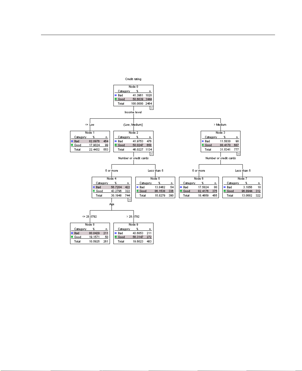
81

Tree Diagram

Figure 4-8

Tree diagram

forcreditratingmodel

Using Classifi

cation Trees to Evaluate Credit Risk

Thetreediagramisagraphicrepresentationofthetreemodel.Thistreediagram
shows that:

 Using the CHAID method, income level is the best predictor of credit rating.
 For the low income category, income level is the only significant predictor of

credit rating. Of the bank customers in this category, 82% have defaulted on
loans. Since there are no child nodes below it, this is considered a terminal node.

 For the medium and high income categories, the next best predictor is number

of credit cards.

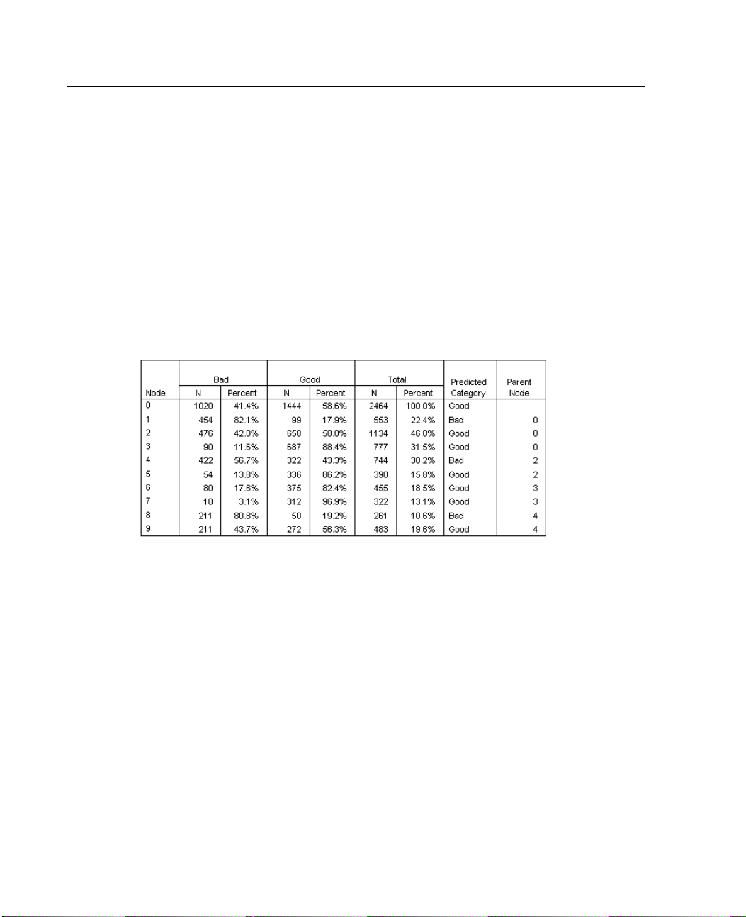
82

Chapter 4



For medium income customers with five or more credit cards, the model includes

one more pre

dictor: age. Over 80% of those customers 28 or younger have a bad

credit rating, while slightly less than half of those over 28 have a bad credit rating.

Tree Table

You can use th

e Tree Editor to hide and show selected branches, change colors and
fonts, and select subsets of cases based on selected nodes. For more information, see
“Selecting Cases in Nodes” on p. 89.

Figure 4-9

Tree table f

or credit r ating

The tree table, as the name suggests, provides most of the essential tree diagram
information in the form of a table. For each node, the table displays:

 The number and percentage of cases in each category of the dependent variable.
 The predicted category for the dependent variable. In this example, the predicted

category is the credit rating category with more than 50% of cases in that node,
since there are only two possible credit ratings.

 The parent node for each node in the tree. Note that node 1—the low income

level node—is not the parent node of any node. Since it is a terminal node,
it has no child nodes.

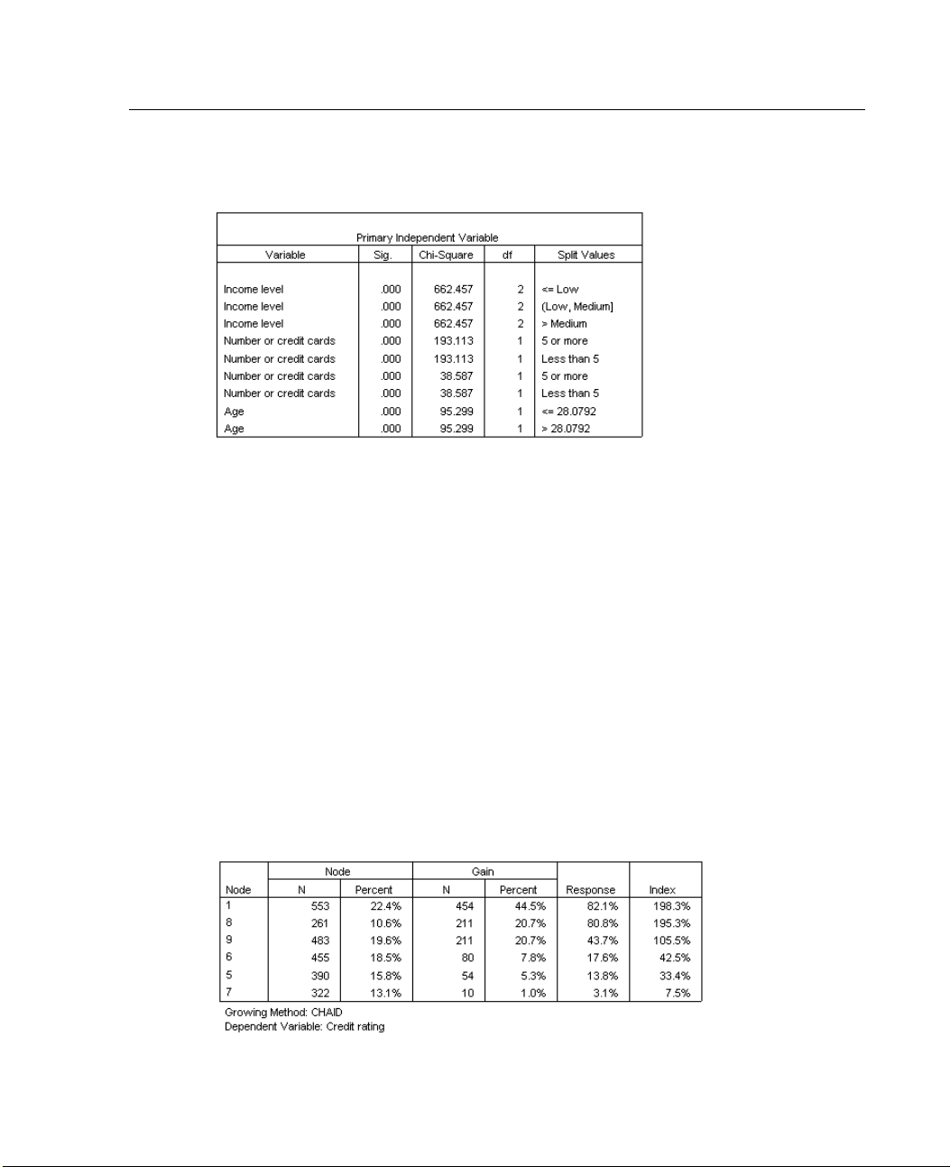
83

Using Classifi

Figure 4-10

Tree table for credit rating (con tinued)

 The independent variable used to split the node.
 The chi-square value (since the tree was generated with the CHAID method),

cation Trees to Evaluate Credit Risk

degrees of freedom ( df), and significance level (Sig.) for the split. For most
practica

l purposes, you will probably be interested only in the significance level,

which is less than 0.0001 for all splits in this model.

 The value(s) of the independent variable for that node.

Note: For ordinal and scale independent variables, you may see ranges in the tree
and tree ta

ble expressed in the general form (value1, value2], which basically means
“greater than value1 and less than or equal to value2.” In this example, income level
has only three possible values—Low, Medium,andHigh—and (Low, Medium] simply
means Med

ium. In a similar fashion, >Medium means High.

Gains for Nodes

Figure 4-11

Gains for nodes

84

Chapter 4

The gains for nodes table provides a summary of information about the terminal
nodes in the model.

 Only the terminal nodes—nodes at which the tree stops growing—are listed in

this table. Frequently, you will be interested only in the terminal n odes, since
they represe

 Since gain v

nt the best classification predictions for the model.

alues provide information about target categories, this table is
available only if you specified one or more target categories. In this example,
there is only one target category, so there is only one gains for nodes table.

 Node N is the number of cases in each terminal node, and Node Percent is the

percentage o

 Gain N is the

f the total number of cases in each node.

number of cases in each terminal node in the target category, and
Gain Percent is the percentage of cases in the target category with respect to the
overall number of cases in the target category—in this example, the number and
percentage

 For categor

of cases with a bad credit rating.

ical dependent variables, Response is the percentage of cases in
the node in the specified target category. In this example, these are the same
percentages displayed for the Bad category in the tree diagram.

 For categorical dependent variables, Index is the ratio of the response percentage

for the targe

t category compared to the response percentage for the entire sample.

Index Values

The index value is basically an indication of how far the observed target category
percentage f

or that node differs from the expected percentage for the target category.
The target category percentage in the root node represents the expected percentage
before the effects of any of the independent variables are considered.

An index val

ue of greater than 100% means that there are more cases in the target
category than the overall percentage in the target category. Conversely, an index
value of less than 100% means there are fewer cases in the target category than
the overal

l percentage.

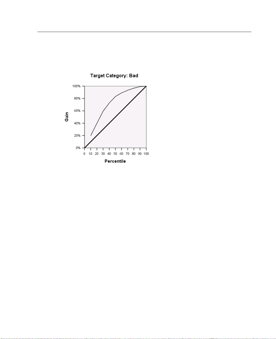
85

Gains Chart

Figure 4-12

Gains chart f

This gains chart indicates that the model is a fairly good one.
Cumulative gains charts always start at 0% and end at 100% as you go from one end

to the ot
leveloff. A model that provides no information will follow the diagonal reference line.

Using Classifi

or bad credit rating target category

cation Trees to Evaluate Credit Risk

her. For a good model, the gains chart will rise steeply toward 100% and then

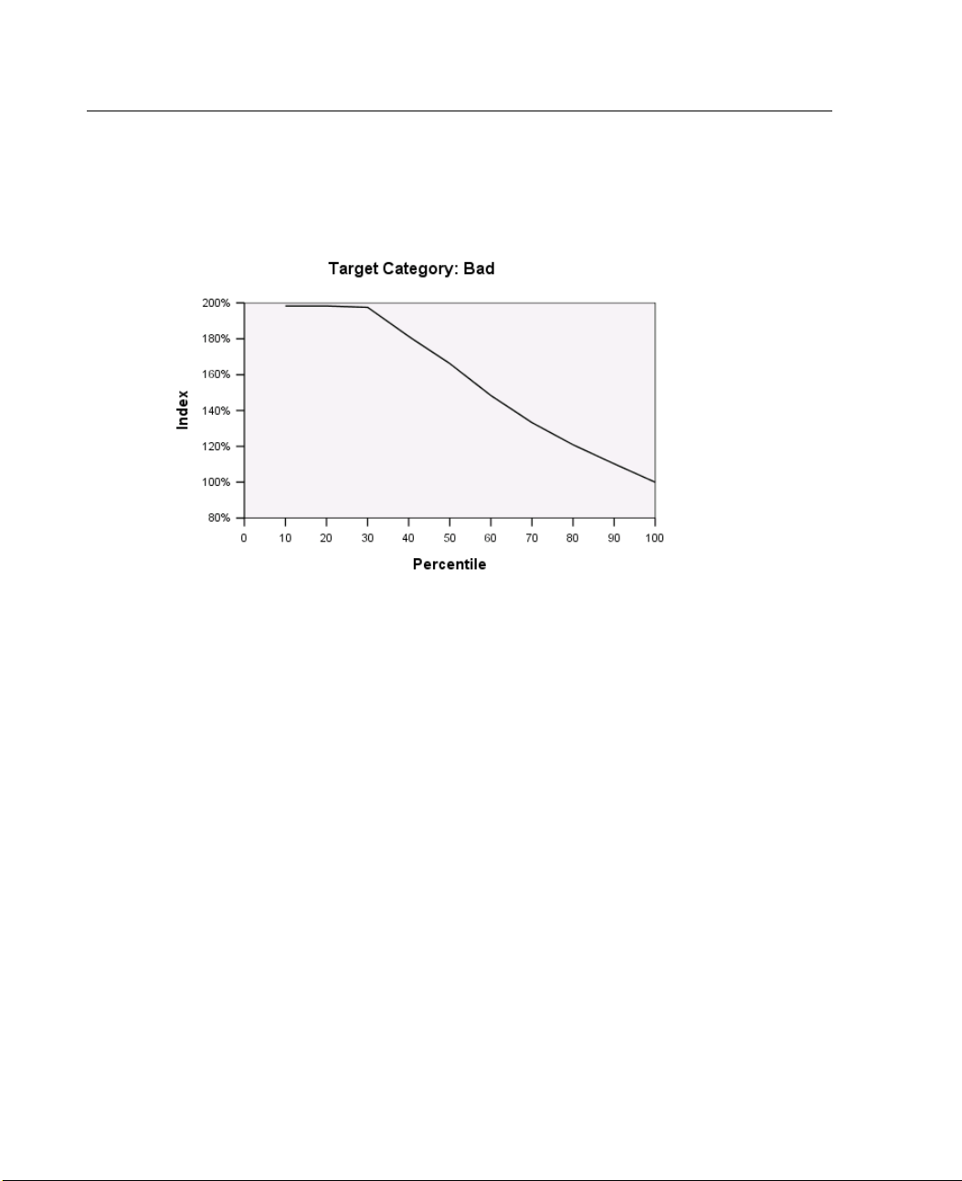
86

Chapter 4

Index Chart

Figure 4-13

Index chart f

or bad credit rating target category

The index chart also indicates that the model is a good one. Cumulative index charts
tend to start above 100% and gradually descend until they reach 100%.

For a goo

d model, the index value should start well above 100%, remain on a high
plateau as you move along, and then trail off sharply toward 100%. For a model that
provides no information, the line will hover around 100% for the entire chart.

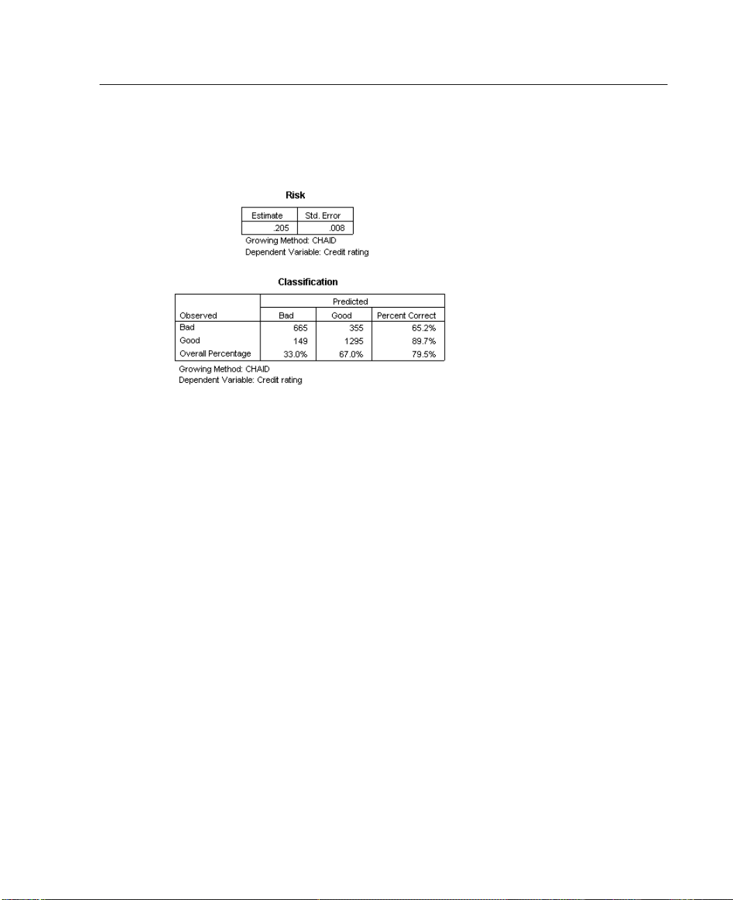
87

Risk Estimate and Classification

Figure 4-14

Risk and clas

The risk a
works.

 The risk estimate of 0.205 indicates that the category predicted by the model

(good or b
misclassifying a customer is approximately 21%.

 The results in the classification table are consistent with the risk estimate. The

table shows that the model classifies approximately 79.5% of the customers
correctl

sification tables

nd classification tables provide a quick evaluation of how well the model

ad credit rating) is wrong for 20.5% of the cases. So the “risk” of

y.

Using Classifi

cation Trees to Evaluate Credit Risk

The classification table does, however, reveal one potential problem with this model:
for those customers with a bad credit rating, it predicts a bad rating for only 65% of
them, whi

ch means that 35% of customers with a bad credit rating are inaccurately

classified with the “good” customers.

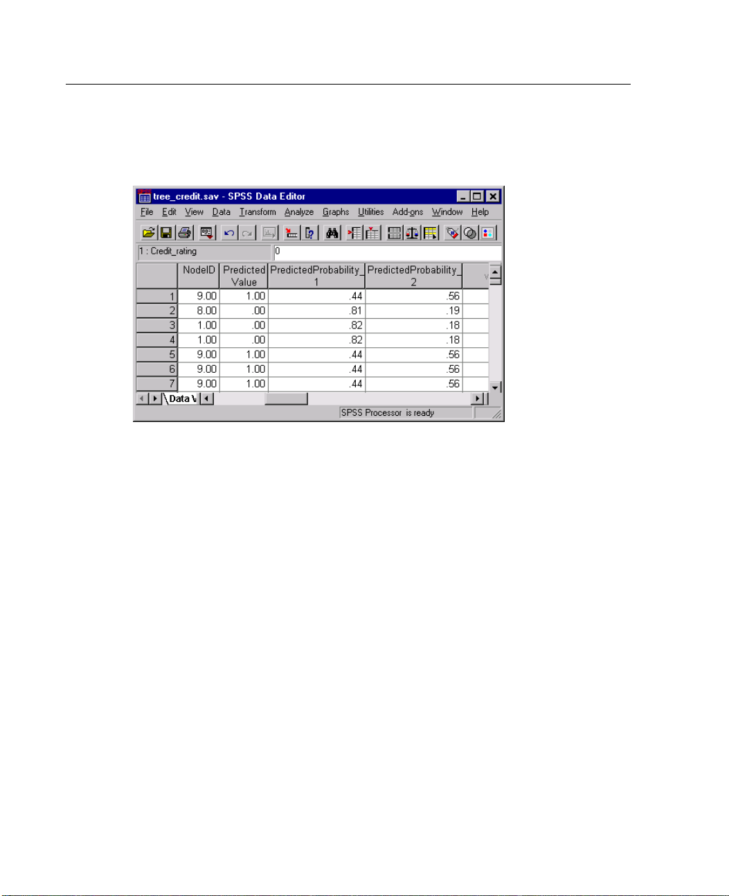
88

Chapter 4

Predicted Values

Figure 4-15

New variable

s for predicted values and probabilities

Four new variables have been created in the working data file:

NodeID. The terminal node number for each case.
PredictedValue. The predicted value of the dependent variable for each case. Since

the dependent variable is coded 0 = Bad and 1 = Good, a predicted value of 0 means
that the case is predicted to have a bad credit rating.

PredictedProbability. The probability that the case belongs in each category of the

dependent variable. Since there are only two possible values for the dependent
variable, two variables are created:

 PredictedProbability_1. The probability that the case belongs in the bad credit

rating category.

 PredictedProbability_2. The probability that the case belongs in the good credit

rating category.

The predicted probability is simply the proportion of cases in each category of the
dependent variable for the terminal node that contains each case. For example, in
node 1, 82% of the cases are in the bad category and 18% are in the good category,
resulting in predicted probabilities of 0.82 and 0.18, respectively.

89

For a categorical dependent variable, the predicted value is the category with the
highest proportion of cases in the terminal node for each case. For example, for the
first case,

the predicted value is 1 (good credit rating), since approximately 56% of
the cases in its terminal node have a good credit rating. Conversely, for the second
case, the predicted value is 0 (bad credit rating), since approximately 81% of cases in
its termin

al node have a bad credit rating.

If you have defined costs, however, the relationship between predicted category and
predicted probabilities may not be quite so straightforward. For more information,
see “Assig

ning Costs to Outcomes” on p. 95.

Refining the Model

Overall, the model has a correct classification rate of just under 80%. This is reflected
in most of
in the node—is the same as the actual category for 80% or more of the cases.

There is, however, one terminal node where cases are fairly evenly split between good
and bad cr
of the cases in that node actually have a good credit rating. That means that almost
half of the cases in that node (44%) will havethe wrong predicted category. And if the
primary c

the terminal nodes, where the predicted category—the highlighted category

edit ratings. In node 9, the predicted credit rating is “good,” but only 56%

oncern is identifying bad credit risks, this node doesn’t perform very well.

Using Classifi

cation Trees to Evaluate Credit Risk

Selecting Cases in Nodes

Let’s look at the cases in node 9 to see if the data reveal any useful additional
informa

E Double
E Click no
E From the

Rules

tion.

-clickthetreeintheViewertoopentheTreeEditor.
de 9 to select it. (If you want to select multiple nodes, use Ctrl-click).

Tree Editor menus choose:

Filter Cases...

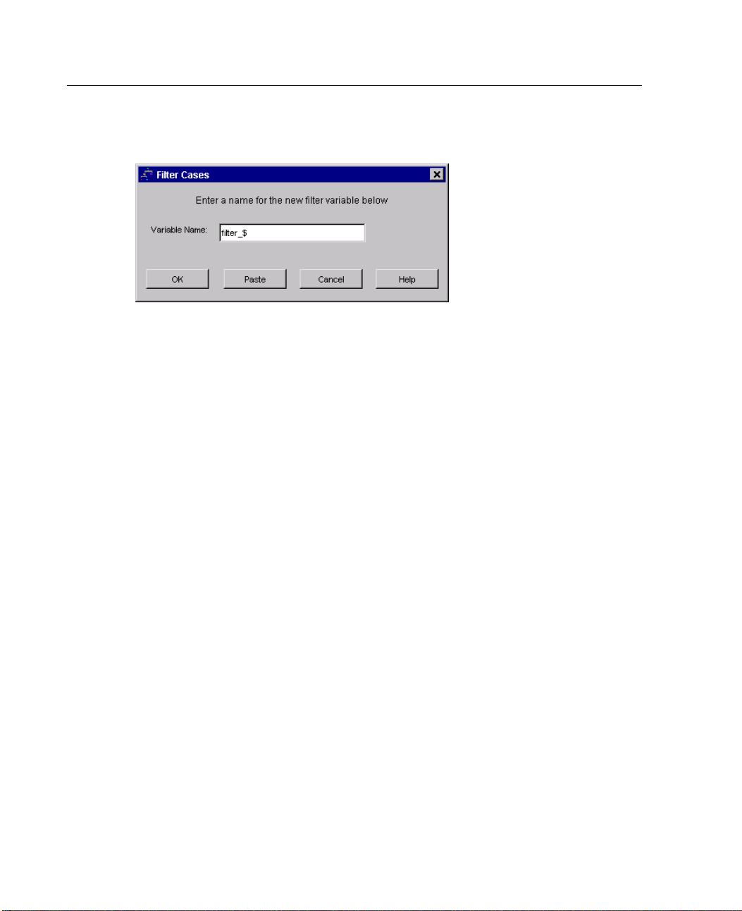
90

Chapter 4

Figure 4-16

Filter Cases dialog box

The Filter Cases dialog box will create a filter variable and apply a filter setting based
on the valu

 Cases fro
 All other c

es of that variable. The default filter variable name is filter_$.

m the selected nodes will receive a value of 1 for the filter variable.

ases will receive a value of 0 and will be excluded from subsequent

analyses until you change the filter status.

In this exam

ple, that means cases that aren’t in node 9 will be filtered out (but not

deleted) for now.

E Click OK to create the filter variable and apply the filter condition.