

Page 1
SPSS Categories® 13.0
Jacqueline J. Meulman
Jacqueline J. Meulman
Willem J. Heiser
Willem J. Heiser
SPSS Inc
SPSS Inc
Page 2

For more information about SPSS®software products, please visit our Web site at http://www.spss.com or contact
SPSS Inc.
233 South Wacker Drive, 11th Floor
Chicago, IL 60606-6412
Tel: (312) 651
Fax: (312) 651-3668
SPSS is a registered trademark and t he other product names are the t rademarks of SPSS Inc. for its proprietary computer
software. No m
the trademark and license rights in the software and the copyrights in the published materials.
The SOFTWARE and documentation are provided with RESTRICTED R IGHTS. Use, duplication , or disclosure by the
Governmentis
clause at 52.227-7013. Contractor/manufacturer is SPSS Inc., 233 South Wacker Drive, 11th Floor, Chicago, IL 60606-6412.
General notice: Other product names mentioned herein are used for identification purposes only and may be trademarks of
their respec
TableLook is a trademark of SPSS Inc.
Windows is a registered trademark of Microsoft Corporation.
DataDirect, D
Portions of this product were created using LEADTOOLS © 1991–2000, LEAD Technologies, Inc. ALL RIGHTS RESERVED.
LEAD, LEADTOOLS, and LEADVIEW are registered trademarks of LEAD Technologies, Inc.
Sax Basic is a t
All rights reserved.
Portions of this product were based on the work of the FreeType Team (http://www.freetype.org).
A portion of th
software is provided “as is,” without express or implied warranty.
A portion of the SPSS software contains Sun Java Runtime libraries. Copyright © 2003 by Sun Microsystems, Inc. All rights
reserved. The
licensed from IBM and are available at http://oss.software.ibm.com/icu4j/.
SPSS Categories® 13.0
Copyright © 20
All rights reserved.
Printed in the United States of America.
No part of this p
electronic, mechanical, photocopying, recording, or otherwise, without the prior written permission of the publisher.
1234567890 07060504
ISBN 1-56827-
-3000
aterial describing such software may be produced or distributed without the written permission of the owners of
subject to restrictions as set forth in subdivision (c) (1) (ii) of The Rights in Technical Data and Computer Software
tive companies.
ataDirect Connect, INTERSOLV, and SequeLink are registered trademarks of DataDirect Technologies.
rademark of Sax Software Corporation. Copyright © 1993–2004 by Polar Engineering and Consulting.
e SPSS software contains zlib technology. Copyright © 1995–2002 by Jean-loup Gailly and Mark Adler. The zlib
Sun Java Runtime libraries include code licensed from RSA Security, Inc. Some portions of the libraries are
04 by SPSS Inc.
ublication may be reproduced, stored in a retrieval system, or transmitted, in any form or by any means,
351-7
Page 3

Preface
SPSS 13.0 is a comprehensive system for analyzing data. The Categories optional
add-on mod
The Categories add-on module must be used with the SPSS 13.0 Base system and is
completely integrated into that system.
Installation
To install the Categories add-on module, run the License Authorization Wizard using
the authorization code that you received from SPSS Inc. For more information, see
the insta
Compatibility
SPSS is designed to run on many computer systems. See the installation instructions
that cam
requirements.
ule provides the additional analytic techniques described in this manual.
llation instructions supplied with the SPSS Base system.
e with your system for specific information on minimum and recommended
Serial N
Your ser
this serial number when you contact SPSS Inc. for information regarding support,
payment, or an upgraded system. The serial number was provided with your Base
system
Customer Service
If you have any questions concerning your shipment or account, contact your local
office
your serial number ready for identification.
umbers
ial number is your identification number with SPSS Inc. You will need
.
, listed on the SPSS Web site at http://www.spss.com/worldwide. Please have
iii
Page 4

Training Seminars
SPSS Inc. provides both public and onsite training seminars. All seminars feature
hands-on workshops. Seminars will be offered in major cities on a regular basis. For
more informa
tion on these seminars, contact your local office, listed on the SPSS
Web site at http://www.spss.com/worldwide.
Technical S
The service
upport
s of SPSS Technical Support are available to registered customers.
Customers may contact Technical Support for assistance in using SPSS or for
installation help for one of the supported hardware environments. To reach Technical
Support, s
ee the SPSS Web site at http://www.spss.com, or contact your local office,
listedontheSPSSWebsiteathttp://www.spss.com/worldwide.Bepreparedto
identify yourself, your organization, and the serial number of your system.
Additional Publications
Additional copies of SPSS product manuals may be purchased directly from SPSS
Inc. Visit the SPSS Web Store at http://www.spss.com/estore, or contact your local
SPSS offi
ce, listed on the SPSS Web site at http://www.spss.com/worldwide.For
telephone orders in the United States and Canada, call SPSS Inc. at 800-543-2185.
For telephone orders outside of North America, contact your local office, listed
on the SP
SS Web site.
The SPSS Statistical Procedures Companion, by Marija Norušis, has been
published by Prentice Hall. A new version of this book, updated for SPSS 13.0, is
planned
.TheSPSS Advanced Statistical Procedures Companion,alsobasedon
SPSS 13.0, is forthcoming. The SPSS Guide to Data Analysis for SPSS 13.0 is also in
development. Announcements of publications available exclusively through Prentice
Hall wi
your home country, and then click
ll be available on the SPSS Web site at http://www.spss.com/estore (select
Books).
Tel l Us
Your co
Your Thoughts
mments are important. Please let us know about your experiences with SPSS
products. We especially like to hear about new and interesting applications using
the SPSS system. Please send e-mail to [email protected] or write to SPSS Inc.,
iv
Page 5

Attn.: Director of Product Planning, 233 South Wacker Drive, 11th Floor, Chicago,
IL 60606-6412.
About This Manual
This manual documents the graphical user interface for the procedures included in
the Categories add-on module. Illustrations of dialog boxes are taken from SPSS for
Windows. Di
alog boxes in other operating systems are similar. Detailed information
about the command syntax for features in this module is provided in the SPSS
Command Syntax Reference, available from the Help menu.
Contacting SPSS
If you would like to be on our mailing list, contact one of our offices, listed on our
Web site at http://www.spss.com/worldwide.
Acknowledgments
The optimal scaling procedures and their SPSS implementation were developed
by the Data Theory Scaling System Group (DTSS), consisting of members of the
departme
nts of Education and Psychology of the Faculty of Social and Behavioral
Sciences at Leiden University.
Willem Heiser, Jacqueline Meulman, Gerda van den Berg, and Patrick Groenen
were invo
lved with the original 1990 procedures. Jacqueline Meulman and
Peter Neufeglise participated in the development of procedures for categorical
regression, correspondence analysis, categorical principal components analysis, and
multidi
mensional scaling. In addition, Anita van der Kooij contributed especially
to CATREG, CORRESPONDENCE, and CATPCA,andFrankBusingandWillem
Heiser, to the PROXSCAL procedure. The development of PROXSCAL has profited
from tec
hnical comments and suggestions from Jacques Commandeur and Patrick
Groenen.
v
Page 6

Page 7

Contents
Part I: User
's Guide
1 I ntroduction to SPSS O ptimal Scaling
Procedures for Categorical Data 1
WhatIsOptimalScaling?....................................... 1
WhyUseOptimalScaling? ...................................... 2
OptimalScalingLevelandMeasurementLevel ...................... 2
SelectingtheOptimalScalingLevel............................ 3
Tran sfor
CategoryCodes .......................................... 5
Which Proc
Categoric
CategoricalPrincipalComponentsAnalysis .................... 10
NonlinearCanonicalCorrelationAnalysis ...................... 11
Correspon
MultipleCorrespondenceAnalysis ........................... 14
MultidimensionalScaling .................................. 15
AspectRatioinOptimalScalingCharts ........................... 16
RecommendedReadings ...................................... 16
mationPlots . ... ... ... ... ... ... ... ... ... ... ... ... .. 4
edureIsBestforYourApplication? ...................... 8
alRegression..................................... 9
denceAnalysis.................................. 12
2 Categoric
CategoricalRegression ....................................... 19
DefineScaleinCategoricalRegression ........................... 21
CategoricalRegressionDiscretization ............................ 23
al Regression (CATREG) 19
vii
Page 8

CategoricalRegressionMissingValues ........................... 24
CategoricalRegressionOptions ................................. 25
CategoricalRegressionOutput.................................. 26
CategoricalRegressionSave................................... 28
CategoricalRegressionTransformationPlots....................... 29
CATREGCommandAdditionalFeatures............................ 29
3 Categorica
l Principal Components Analysis
(CATPCA) 31
DefineScaleandWeightinCATPCA.............................. 34
Categorical Princ ipal Components Analysis Discretization . . . . . . . . . . . . . 36
Categorical Princ ipal Components Analysis Missing Values . . . . . . . . . . . . 38
Categorical Princ ipal Components Analysis Options . . . . . . . . . . . . . . . . . . 39
Categorical Princ ipal Components Analysis Output . . . . . . . . . . . . . . . . . . . 42
Categorical Princ ipal Components Analysis Save . . . . . . . . . . . . . . . . . . . . 44
Categorical Princ ipal Components Analysis Object Plots. . . . . . . . . . . . . . . 45
Categorical Princ ipal Components Analysis Category Plots. . . . . . . . . . . . . 46
Categorical Princ ipal Components Analysis Loadin g Plots . . . . . . . . . . . . . 47
CATPCACommandAdditionalFeatures............................ 48
4 Nonlinear Canonical Correlation Analysis
(OVERALS) 4
Nonlinear
Define Ran
Define Ran
CanonicalCorrelationAnalysis.......................... 49
geandScale....................................... 53
ge............................................... 54
9
viii
Page 9

NonlinearCanonicalCorrelationAnalysisOptions ................... 54
OVERALSCommandAdditionalFeatures........................... 56
5 Correspond
DefineRowRangeinCorrespondenceAnalysis..................... 61
DefineColumnRangeinCorrespondenceAnalysis................... 62
CorrespondenceAnalysisModel ................................ 63
CorrespondenceAnalysisStatistics.............................. 66
CorrespondenceAnalysisPlots ................................. 67
CORRESPONDENCECommandAdditionalFeatures................... 68
6 Multiple C
Define Variable Weight in Multiple Correspondence Analysis . . . . . . . . . . . 73
MultipleCorrespondenceAnalysisDiscretization.................... 74
MultipleCorrespondenceAnalysisMissingValues................... 75
MultipleCorrespondenceAnalysisOptions......................... 77
MultipleCorrespondenceAnalysisOutput ......................... 80
MultipleCorrespondenceAnalysisSave........................... 82
MultipleCorrespondenceAnalysisObjectPlots..................... 82
MultipleCorrespondenceAnalysisVariablePlots.................... 83
MULTIPLE CORRESPONDENCE Command Additional Features . . . . . . . . . . 85
ence Analysis 59
orrespondence Analysis 71
7 Multidime
ProximitiesinMatricesacrossColumns........................... 90
nsional Scaling (PROXSCAL) 87
ix
Page 10

ProximitiesinColumns........................................ 91
ProximitiesinOneColumn ..................................... 92
CreateProximitiesfromData ................................... 93
MeasuresDialogBox......................................... 94
DefineaMultidimensionalScalingModel.......................... 95
MultidimensionalScalingRestrictions ............................ 97
MultidimensionalScalingOptions................................ 98
MultidimensionalScalingPlots,Version1.......................... 99
MultidimensionalScalingPlots,Version2......................... 101
MultidimensionalScalingOutput ............................... 101
PROXSCALCommandAdditionalFeatures ........................ 103
Part II: Exam
ples
8 Categorical Regression 107
Example: C
Example: Oz
RecommendedReadings ..................................... 157
arpetCleanerData ................................. 107
A Sta ndard L
ACategoricalRegressionAnalysis .......................... 117
Discretizi
SelectionofTransformationType............................ 132
OptimalityoftheQuantifications ............................ 145
Effects of T
inearRegressionAnalysis....................... 108
oneData........................................ 130
ngVariables .................................... 131
ransformations................................. 148
x
Page 11

9 Categorical
Example: Examining Interrelations of Social Systems . . . . . . . . . . . . . . . . 159
RunningtheAnalysis..................................... 160
NumberofDimensions ................................... 165
Quantifica
ObjectScores.......................................... 169
ComponentLoadings..................................... 170
Additional D
Example:SymptomatologyofEatingDisorders..................... 175
RunningtheAnalysis..................................... 177
Transformat
ModelSummary ........................................ 194
ComponentLoadings..................................... 194
Object Score s
ExaminingtheStructureoftheCourseofIllness ................ 198
Recommended R
Principal Components Analysis 159
tions ......................................... 167
imensions.................................... 172
ionPlots..................................... 190
.......................................... 196
eadings ..................................... 213
10 Nonlinear Canonical Correlation Analysis 217
Example: An
Examining t
AccountingforSimilaritybetweenSets....................... 226
ComponentLoadings..................................... 230
Transformat
SingleversusMultipleCategoryCoordinates................... 235
CentroidsandProjectedCentroids........................... 236
An Alternati
GeneralSuggestions..................................... 247
Recommended R
AnalysisofSurveyResults.......................... 217
heData...................................... 218
ionPlots..................................... 231
veAnalysis................................... 241
eadings ..................................... 248
xi
Page 12

11 Corresponde
Normalization.............................................. 250
Example:SmokingBehaviorbyJobCategory...................... 251
RunningtheAnalysis..................................... 252
CorrespondenceTable.................................... 255
Dimensional
Biplot................................................. 257
ProfilesandDistances.................................... 258
Row and Colum
PermutationsoftheCorrespondenceTable.................... 262
ConfidenceStatistics..................................... 263
Supplementa
Example:PerceptionsofCoffeeBrands .......................... 270
RunningtheAnalysis..................................... 271
Dimensionali
Contributions........................................... 277
Plots................................................. 279
Symmetrical N
Example:FlyingMileagebetweenCities.......................... 283
CorrespondenceTable.................................... 292
Row and Column S
RecommendedReadings ..................................... 294
nce Analysis 249
ity.......................................... 256
nScores.................................. 260
ryProfiles................................... 264
ty.......................................... 276
ormalization ................................ 281
cores.................................. 293
12 Multiple Correspondence Analysis 297
Example:CharacteristicsofHardware........................... 297
RunningtheAnalysis..................................... 298
Model Summary
ObjectScores.......................................... 302
DiscriminationMeasures.................................. 304
........................................ 301
xii
Page 13

CategoryQuantifications.................................. 305
AMoreDetailedLookatObjectScores....................... 307
Omission of O
RecommendedReadings ..................................... 315
utliers...................................... 310
13 Multidimensional Scaling 317
Example:AnExaminationofKinshipTerms........................ 317
ChoosingtheNumberofDimensions......................... 318
AThree-Di
A Three-Dimensional Solution with Nondefault Transformations . . . . 335
Discussion............................................. 340
RecommendedReadings ..................................... 341
mensionalSolution.............................. 328
Bibliography 343
Index 351
xiii
Page 14

Page 15
Part 1: User's Guide
Page 16

Page 17

Chapter
1
Introductio
ntoSPSS
Optimal Scaling P rocedures for
Categorical Data
SPSS Categories procedures use optimal scaling to analyze data that are difficult or
impossible for standard statistical procedures to analyze. This chapter describes what
each proc
relationships between the procedures, and the relationships of these procedures to
their standard statistical counterparts.
Note:The
Theory Scaling System Group (DTSS), consisting of members of the departments
of Education and Psychology, Faculty of Social and Behavioral Sciences, Leiden
Univers
What Is Optimal Scaling?
edure does, the situations in which each procedure is most appropriate, the
se procedures and their SPSS implementation were developed by the Data
ity.
The idea behind optimal scaling is to assign numerical quantifications to the
ries of each variable, thus allowing standard procedures to be used to obtain
catego
a solution on the quantified variables.
The optimal scale values are assigned to categories of each variable based on the
zing criterion of the procedure in use. Unlike the original labels of the nominal
optimi
or ordinal variables in the analysis, these scale values have metric properties.
In most Categories procedures, the optimal quantification for each scaled variable
ined through an iterative method called alternating least squares in which,
is obta
after the current quantifications are used to find a solution, the quantifications are
updated using that solution. The updated quantifications are then used to find a new
1
Page 18

2
Chapter 1
solution, which is used to update the quantifications, and so on, until some criterion is
reached that signals the process to stop.
Why Use Optimal Scaling?
Categorical data are often found in marketing research, survey research, and
research in the social and behavioral sciences. In fact, many researchers deal almost
exclusive
data, they often do not perform well for data sets that feature:
Too few observations
Too many variables
Toomanyvaluespervariable
ly with categorical data.
While adaptations of most standard models exist specifically to analyze categorical
By quantify
situations. Moreover, they are useful even when specialized techniques are
appropriate.
output is often based on graphical displays. Optimal scaling techniques offer excellent
exploratory analyses, which complement other SPSS models well. By narrowing the
focus of yo
the basis of an analysis that centers on interpretation of model parameters.
Optimal S
This can b
When specifying the level, you specify not the level at which variables are measured
but the level at which they are scaled. The idea is that the variables to be quantified
may have
For Cate
The nom
ing categories, optimal scaling techniques avoid problems in these
Rather tha
n interpreting parameter estimates, the interpretation of optimal scaling
ur investigation, visualizing your data through optimal scaling can form
caling Level and Measurement Level
e a very confusing concept when you first use Categories procedures.
nonlinear relations regardless of how they are measured.
gories purposes, there are three basic levels of measurement:
inal level implies that a variable’s values represent unordered categories.
Examples of variables that might be nominal are region, zip code area, religious
affiliation, and multiple choice categories.
Page 19

3
Introduction t
The ordinal level implies that a variable’s values represent ordered categories.
Examples in
clude attitude scales representing degree of satisfaction or confidence
o SPSS Optimal Scaling Procedures for Categorical Data
and preference rating scores.
The numerical level implies that a variable’s values represent ordered categories
with a meaningful metric so that distance comparisons between categories are
appropriat
For example
e. Examples include age in years and income in thousands of dollars.
, suppose that the variables region, job,andage are coded as shown
in the following table.
Tab l e 1-1
Coding scheme for region, job , and age
Region Job Age
1 North 1 intern 20 twenty years old
2 South 2 sales rep 22 twenty-two years old
3East 3
4 West 27 twenty-seven years old
manager
twenty-five years old
25
The values shown represent the categories of each variable. Region would be a
nominal variable. There are four categories of region, with no intrinsic ordering.
Values 1
through 4 simply represent the four categories; the coding scheme is
completely arbitrary. Job,ontheotherhand,couldbeassumedtobeanordinal
variable. The original categories form a progression from intern to manager. Larger
codes r
epresent a job higher on the corporate ladder. However, only the order
information is known—nothing can be said about the distance between adjacent
categories. In contrast, age could be assumed to be a numerical variable. In the case
, the distances between the values are intrinsically meaningful. The distance
of age
between 20 and 22 is the same as the distance between 25 and 27, while the distance
between 22 and 25 is greater than either of these.
Selecting the Optimal Scaling Level
It is important to understand that there are no intrinsic properties of a variable that
automatically predefine what optimal scalinglevelyoushouldspecifyforit.Youcan
ore your data in any way that makes sense and makes interpretation easier. By
expl
Page 20

4
Chapter 1
analyzing a numerical-level variable at the ordinal level, for example, the use of a
nonlinear transformation may allow a solution in fewer dimensions.
The followin
g two examples illustrate how the “obvious” level of measurement
might not be the best optimal scaling level. Suppose that a variable sorts objects into
age groups. Although age can be scaled as a numerical variable, it may be true
that for peo
ple younger than 25 safety has a positive relation with age, whereas for
people older than 60 safety has a negative relation with age. In this case, it might be
better to treat age as a nominal variable.
As another
example, a variable that sorts persons by political preference appears
to be essentially nominal. However, if you order the parties from political left to
political right, you might want the quantification of parties to respect this o rder
by using an
ordinal level of analysis.
Even though there are no predefined properties of a variable that make it
exclusively one level or another, there are some general guidelines to help the novice
user. Wit
h single-nominal quantification, you don’t usually know the order of the
categories but you want the analysis to impose one. If the order of the categories is
known, you should try ordinal quantification. If the categories are unorderable, you
might try
multiple-nominal quantification.
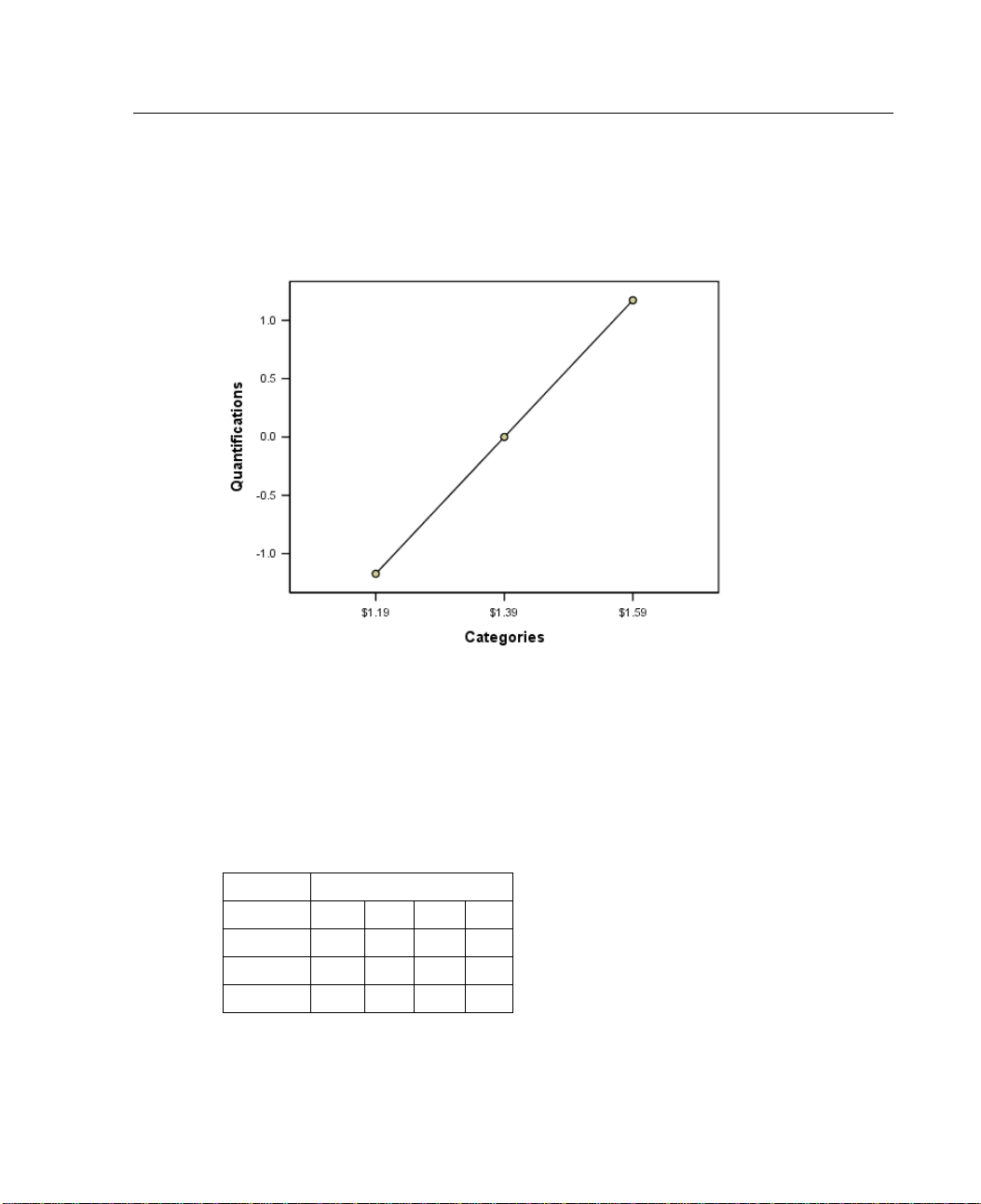
Transformation Plots
The different levels at which each variable can be scaled impose different restrictions
on the qu
quantifications and the original categories resulting from the selected optimal scaling
level. For example, a linear transformation plot results when a variable is treated as
numeri
Transformationplots for variables treated nominally that are U-shaped (or the inverse)
display a quadratic relationship. Nominal variables could also yield transformation
plots w
following figure displays a sample transformation plot.
optim
collapsing these categories into one category may be warranted. Alternatively, if a
variable treated as nominal receives quantifications that display an increasing trend,
an ord
antifications. Transformation plots illustrate the relationship between the
cal. Variables treated as ordinal result in a nondecreasing transformation plot.
ithout apparent trends by changing the order of the categories c ompletely. The
Transformation plots a re particularly suited to determining how well the selected
al scaling level performs. If several categories receive similar quantifications,
inal transformation may result in a similar fit. If that trend is linear, numerical
Page 21
5
Introduction t
o SPSS Optimal Scaling Procedures for Categorical Data
treatment may be appropriate. However, if collapsing categories or changing scaling
levels is warranted, the analysis will not change significantly.
Figure 1-1
Transformation plot of price (numerical)
Category Codes
Somecareshouldbetakenwhencodingcategorical variables because some coding
schemes may yield unwanted output or incomplete analyses. Possible coding schemes
for job
Tab l e 1
ative coding schemes for job
Altern
Category A B C D
intern 1 1
sales rep 2 2 6
manager
are displayed in the following table.
-2
Scheme
1
5
5
3773
Page 22

6
Chapter 1
Some Categories procedures require that the range of every variable used be defined.
Any value outside this range is treated as a missing value. The minimum category
value is alw
ays 1. The maximum category value is supplied by the user. This value
is not the number of categories for a variable—it is the largest category value. For
example, in the table, scheme A has a maximum category value of 3 and scheme B
has a maxim
um category value of 7, yet both schemes code the same three categories.
The variable range determines which categories will be omitted from the analysis.
Any categories with codes outside the defined range are omitted from the analysis.
This is a si
mple method for omitting categories but can result in unwanted analyses.
An incorrectly defined maximum category can omit valid categories from the analysis.
For example, for scheme B, defining the maximum category value to be 3 indicates
that job h
as categories coded from 1 to 3; the manager category is treated as missing.
Because no category has actually been coded 3, the third category in the analysis
contains no cases. If you wanted to omit all manager categories, this analysis would
be appro
priate. However, if managers are to be included, the maximum category must
be defined as 7, and missing values must be coded with values above 7 or below 1.
For variables treated as nominal or ordinal, the range of the categories does not
he results. For nominal variables, only the label and not the value associated
affect t
with that label is important. For ordinal variables, the order of the categories is
preserved in the quantifications; the category values themselves are not important. All
coding
schemes resulting in the same category ordering will have identical results.
For example, the first three schemes in the table are functionally equivalent if job is
analyzed at an ordinal level. The order of the categories is identical in these schemes.
Scheme
D, on the other hand, inverts the second and third categories and will yield
different results than the other schemes.
Although many coding schemes for a variable are functionally equivalent, schemes
mall differences between codes are preferred because the codes have an
with s
impact on the amount of output produced by a procedure. All categories coded
with values between 1 and the user-defined maximum are valid. If any of these
ories are empty, the corresponding quantifications will be either system missing
categ
or zero, depending on the procedure. Although neither of these assignments affect
the analyses, output is produced for these categories. Thus, for scheme B, job has
categories that receive system-missing values. For scheme C, there are also four
four
categories receiving system-missing indicators. In contrast, for scheme A there are no
system-missing quantifications. Using consecutive integers as codes for variables
ated as nominal or ordinal results in much less output without affecting the results.
tre
Page 23

7
Introduction t
o SPSS Optimal Scaling Procedures for Categorical Data
Coding schemes for variables treated as numerical are more restricted than the
ordinal case. For these variables, the differences between consecutive categories are
important.
Tab l e 1-3
Alternativ
Category A B C
Any recod
The following table displays three coding schemes for age.
e coding schemes for age
Scheme
20 20 1 1
22 22 3 2
25 25
27 27 8 4
63
ing of numerical variables must preserve the differences between the
categories. Using the original values is one method for ensuring preservation of
differences. However, this can result in many categories having system-missing
ors. For example, scheme A employs the original observed values. For all
indicat
Categories procedures except for Correspondence Analysis, the maximum category
value is 27 and the minimum category value is set to 1. The first 19 categories are
empty a
nd receive system-missing indicators. The output can quickly become rather
cumbersome if the maximum category is much greater than 1 and there are many
empty categories between 1 and the maximum.
To redu
ce the amount of output, recoding can be done. However, in the numerical
case, the Automatic Recode facility should not be used. Coding to consecutive
integers results in differences of 1 between all consecutive categories, and, as a
t, all quantifications will be equally spaced. The metric characteristics deemed
resul
important when treating a variable as numerical are destroyed by recoding to
consecutive integers. For example, scheme C in the table corresponds to automatically
ding age. The difference between categories 22 and 25 has changed from three to
reco
one, and the quantifications will reflect the latter difference.
An alternative recoding scheme that preserves the differences between categories
subtract the smallest category value from every category and add 1 to each
is to
difference. Scheme B results from this transformation. The smallest category value,
20, has been subtracted from each category, and 1 was added to each result. The
sformed codes have a minimum of 1, and all differences are identical to the
tran
original data. The maximum category value is now 8, and the zero quantifications
before the first nonzero quantification a re all eliminated. Yet, the nonzero
Page 24

8
Chapter 1
quantifications corresponding to each category resulting from scheme B are identical
to the quantifications from scheme A.
Which Procedure Is Best for Your Application?
The techniques embodied in four of these procedures (Correspondence Analysis,
Multiple Correspondence Analysis, Categorical Principal Components Analysis, and
Nonlinear
data analysis known as dimension reduction. That is, relationships between
variables are represented in a few dimensions—say two or three—as often as
possible.
would be too difficult to fathom in their original richness and complexity. In market
research applications, these techniques can be a form of perceptual mapping.A
major adv
levels of optimal scaling.
Categorical Regression describes the relationship between a categorical response
variable
each predictor variable on the response variable is described by the corresponding
regression weight. As in the other procedures, data can be analyzed with different
levels o
Multidimensional Scaling describes relationshipsbetweenobjectsinasfew
dimensions as possible, starting either with a matrix of proximities between the
objects
Canonical Correlation Analysis) fall into the general area of multivariate
This enables you to describe structures or patterns in the relationships that
antage of these procedures is that they accommodate data with different
and a combination of categorical predictor variables. The influence of
f optimal scaling.
or with the original data from which the proximities are computed.
ing are brief guidelines for each of the procedures:
Follow
Use Cat
egorical Regression to predict the values of a categorical dependent
variable from a combination of categorical independent variables.
Use Categorical Principal Components Analysis to account for patterns of
variation in a single set of variables of mixed optimal scaling levels.
Use Nonlinear Canonical Correlation Analysis to assess the extent to which two
or more
Use Co
sets of variables of mixed optimal scaling levels are correlated.
rrespondence Analysis to analyze two-way contingency tables or data that
can be expressed as a two-way table, such as brand preference or sociometric
choice data.
Page 25

9
Use Multidimensional Scaling to analyze proximity data to find a least-squares
Categorica
The use of Ca
is to predict a dependent (response) variable from a set of independent (predictor)
variables. As with all optimal scaling procedures, scale values are assigned to
each categ
to the regression. The solution of a categorical regression maximizes the squared
correlation between the transformed response and the weighted combination of
transfor
Relation to other Categories procedures. Categorical regression with optimal scaling is
comparable to optimal scaling canonical correlation analysis with two sets, one of
which con
is derived by comparing each set to an unknown variable that lies somewhere between
all of the sets. In categorical regression, similarity of the transformed response and
the line
Introduction t
o SPSS Optimal Scaling Procedures for Categorical Data
Use Multiple Correspondence Analysis to analyze a categorical multivariate data
matrix when
you are willing to make no stronger assumption that all variables are
analyzed at the nominal level.
representation of the objects in a low-dimensional space.
l Regression
tegorical Regression is most appropriate when the goal of your analysis
ory of every variable such that these values are optimal with respect
med predictors.
tains only the dependent variable. In the latter technique, similarity of sets
ar combination of transformed predictors is assessed directly.
Relation to standard techniques. In standard linear regression, categorical variables can
either be recoded as indicator variables or be treated in the same fashion as interval
ariables. In the first approach, the model contains a separate intercept and slope
level v
for each combination of the levels of the categorical variables. This results in a large
number of parameters to interpret. In the second approach, only one parameter is
ted for each variable. However, the arbitrary nature of the category codings
estima
makes generalizations impossible.
If some of the variables are not continuous, alternative analyses are available. If
sponse is continuous and the predictors are categorical, analysis of variance
the re
is often employed. If the response is categorical and the predictors are continuous,
logistic regression or discriminant analysis may be appropriate. I f the response and
edictors are both categorical, loglinear models are often used.
the pr
Page 26

10
Chapter 1
Regression with optimal scaling offers three scaling levels for each variable.
Combinations of these levels can account for a wide range of nonlinear relationships
for which an
offers greater flexibility than the standard approaches with minimal added complexity.
In addition, nonlinear transformations of the predictors usually reduce the
dependenci
matrix for the predictors with the eigenvalues of the correlation matrix for the
optimally scaled predictors, the latter set will usually be less variable than the former.
In other wo
of the predictor correlation matrix smaller and the smaller eigenvalues larger.
y single “standard” method is ill-suited. Consequently, optimal scaling
es among the predictors. If you compare the eigenvaluesof the correlation
rds, in categorical regression, optimal scaling makes the larger eigenvalues
Categoric
al Principal Components Analysis
The use of
you want to account for patterns of variation in a single set of variables of mixed
optimal scaling levels. This technique attempts to reduce the dimensionality of
asetofva
values are assigned to each category of every variable so that these values are optimal
with respect to the principal components solution. Objects in the analysis receive
compone
patterns among the objects in the analysis and can reveal unusual objects in the
data. The solution of a categorical principal components analysis maximizes the
correl
of components (dimensions) specified.
An important application of categorical principal components is to examine
prefer
preference. In the usual SPSS data configuration, rows are individuals, columns are
measurements for the items, and the scores across rows are preference scores (on a 0
to 10 s
may want to treat the individuals as variables. Using the Transpose procedure, you
can transpose the data. The raters become the variables, and all variables are declared
nal. There is no objection to using more variables than objects in CATPCA.
ordi
Relation to other Categories procedures. If all variables are declared multiple nominal,
categorical principal components analysis produces an analysis equivalent to a
mult
Categorical Principal Components Analysis is most appropriate when
riables while accounting for as much of the variation as possible. Scale
nt scores based on the quantified data. Plots of the component scores reveal
ations of the object scores with each of the quantified variables for the number
ence data, in which respondents rank or rate a number of items with respect to
cale, for example), making the data row-conditional. For preference data, you
iple correspondence analysis run on the same variables. Thus, categorical
Page 27

11
Nonlinear
Introduction t
o SPSS Optimal Scaling Procedures for Categorical Data
principal components analysis can be seen as a type of multiple correspondence
analysis in which some of the variables are declared ordinal or numerical.
Relation to
standard techn iques.
If all variables are scaled on the numerical level,
categorical principal components analysis is equivalent to standard principal
components analysis.
More genera
lly, categorical principal components analysis is an alternative to
computing the correlations between non-numerical scales and analyzing them using a
standard principal components or factor-analysis approach. Naive use of the usual
Pearson co
rrelation coefficient as a measure of association for ordinal data can lead to
nontrivial bias in estimation of the correlations.
Canonical Correlation Analysis
Nonlinear
different applications. The goal of nonlinear canonical correlation analysis is to
analyze the relationships between two or more sets of variables instead of between
the varia
may have two sets of variables, where one set of variables might be demographic
background items on a set of respondents and a second set might be responses to a
set of at
ordinal, and numerical. Optimal scaling canonical correlation analysis determines the
similarity among the sets by simultaneously comparing the canonical variables from
each se
Canonical Correlation Analysis is a very general procedure with many
bles themselves, as in principal components analysis. For example, you
titude items. The scaling levels in the analysis can be any mix of nominal,
t to a compromise set of scores assigned to the objects.
Relation to other Categories procedures. If there are two or more sets of variables
with only one variable per set, optimal scaling canonical correlation analysis is
lent to optimal scaling principal components analysis. If all variables in
equiva
a one-variable-per-set analysis are multiple nominal, optimal scaling canonical
correlation analysis is equivalent to multiple correspondence analysis. If there are two
f variables, one of which contains only one variable, optimal scaling canonical
sets o
correlation analysis is equivalent to categorical regression with optimal scaling.
Relation to standard techniques. Standard canonical correlation analysis is a statistical
ique that finds a linear combination of one set of variables and a linear
techn
combination of a second set of variables that are maximally correlated. Given
this set of linear combinations, canonical correlation analysis can find subsequent
Page 28

12
Chapter 1
independent sets of linear combinations, referred to as canonical variables, up to a
maximum number equal to the number of variables in the smaller set.
If there are t
wo sets of variables in the analysis and all variables are defined to be
numerical, optimal scaling canonical correlation analysis is equivalent to a standard
canonical correlation analysis. Although SPSS does not have a canonical correlation
analysis pr
ocedure, many of the relevant statistics can be obtained from multivariate
analysis of variance.
Optimal scaling canonical correlation analysis has various other applications.
If you have
two sets of variables and one of the sets contains a nominal variable
declared as single nominal, optimal scaling canonical correlation analysis results can
be interpreted in a similar fashion to regression analysis. If you consider the variable
to be multi
ple nominal, the optimal scaling analysis is an alternative to discriminant
analysis. Grouping the variables in more than two sets provides a variety of ways
to analyze your data.
Correspondence Analysis
The goal of correspondence analysis is to make biplots for correspondence tables.
In a correspondence table, the row and column variables are assumed to represent
unorder
Both variables are inspected for their nominal information only. That is, the only
consideration is the fact that some objects are in the same category while others
are not.
same variable.
tables
in the correspondence analysis solution is the minimum of r minus 1 or c minus 1,
whichever is less. In other words, you could perfectly represent the row categories or
the col
speaking, however, you would like to represent the row and column categories of
a two-way table in a low-dimensional space, say two dimensions, for the reason
that t
spatial representations.
stati
are represented in the low-dimensional representation. Provided that the quality of
ed categories; therefore, the nominal optimal scaling level is always used.
Nothing is assumed about the distance or order between categories of the
One specific use of correspondence analysis is the analysis of two-way contingency
.Ifatablehasr active rows and c active columns, the number of dimensions
umn categories of a contingency table in a space of dimensions. Practically
wo-dimensional plots are more easily comprehensible than multidimensional
When fewer than the maximum number of possible dimensions is used, the
stics produced in the analysis describe how well the row and column categories
Page 29

13
Introduction t
o SPSS Optimal Scaling Procedures for Categorical Data
representation of the two-dimensional solution is good, you can examine plots of the
row points and the column points to learn which categories of the row variable are
similar, wh
ich categories of the column variable are similar, and which row and
column categories are similar to each other.
Relation to other Categories procedures. Simple correspondence analysis is limited to
two-way tab
les. If there are more than two variables of interest, you can combine
variables to create interaction variables. For example, for the variables region, job,
and age, you can combine region and job to create a new variable rejob with the 12
categorie
s shown in the following table. This new variable forms a two-way table
with age (12 rows, 4 columns), which can be analyzed in correspondence analysis.
Tab l e 1-4
Combinations of region and job
Category Code Category Definition Category Code Category Definition
1 North, intern 7 East, intern
2 North, sales rep 8 East, sales rep
3 North, manager 9 East, manager
4 South, intern 10 West, intern
5
6 South, manager 12 West, manager
South, sales rep 11 West, sales rep
One shortcoming of this approach is that any pair of variables can be combined. We
can combine job and age, yielding another 12-category variable. Or we can combine
and age, which results in a new 16-category variable. Each of these interaction
region
variables forms a two-way table with the remaining variable. Correspondence
analyses of these three tables will not yield identical results, yet each is a valid
ach. Furthermore, if there are four or more variables, two-way tables comparing
appro
an interaction variable with another interaction variable can be constructed. The
number of possible tables to analyze can get quite large, even for a few variables. You
elect one of these tables to analyze, or you can analyze all of them. Alternatively,
can s
the Multiple Correspondence Analysis procedure can be used to examine all of the
variables simultaneously without the need to construct interaction variables.
tion to standard techniques.
Rela
The SPSS Crosstabs procedure can also be used to
analyze contingency tables, with independence as a common focus in the analyses.
However, even in small tables, detecting the cause of departures from independence
be difficult. The utility of correspondence analysis lies in displaying such
may
Page 30

14
Chapter 1
patterns for two-way tables of any size. If there is an association between the row
and column variables—that is, if the chi-square value is significant—correspondence
analysis ma
y help reveal the nature of the relationship.
Multiple Correspondence Analysis
Multiple Correspondence Analysis tries to produce a solution in which o bjects within
thesameca
are plotted far apart. Each object is as close as possible to the category points of
categories that apply to the object. In this way, the categories divide the objects into
homogeneo
objects in the same categories into the same subgroups.
For a one-dimensional solution, multiple correspondence analysis assigns optimal
scale val
that overall, on average, the categories have maximum spread. For a two-dimensional
solution, multiple correspondence analysis finds a second set of quantifications of the
categori
spread, and so on. Because categories of a variable receive as many scorings as there
are dimensions, the variables in the analysis are assumed to be multiple nominal in
optimal
Multiple correspondence analysis also assigns scores to the objects in the analysis
in such a way that the category quantifications are the averages, or centroids, of the
object s
tegory are plotted close together and objects in different categories
us subgroups. Variables are considered homogeneous when they classify
ues (category quantifications) to each category of each variable in such a way
es of each variable unrelated to the first set, attempting again to maximize
scaling level.
cores of objects in that category.
Relation to other Categories procedures. Multiple correspondence analysis is also
known as homogeneity analysis or dual scaling. It gives comparable, but not
cal, results to correspondence analysis when there are only two variables.
identi
Correspondence analysis produces unique output summarizing the fit and quality of
representation of the solution, including stability information. Thus, correspondence
sis is usually preferable to multiple correspondence analysis in the two-variable
analy
case. Another difference between the two procedures is that the input to multiple
correspondence analysis is a data matrix, where the rows are objects and the columns
riables, while the input to correspondence analysis can be the same data matrix,
are va
a general proximity matrix, or a joint contingency table, which is an aggregated
matrix in which both the rows and columns represent categories of variables. Multiple
espondence analysis can also be thought of as principal components analysis of
corr
data scaled at the multiple nominal level.
Page 31

15
Multidi
Introduction t
Relation to standard techniques. Multiple correspondence analysis can be thought of
o SPSS Optimal Scaling Procedures for Categorical Data
as the analysis of a multiway contingency table. Multiway contingency tables can
also be anal
yzed with the SPSS Crosstabs procedure, but Crosstabs gives separate
summary statistics for each category of each control variable. With multiple
correspondence analysis, it is often possible to summarize the relationship between
all of the v
ariables with a single two-dimensional plot. An advanced use of multiple
correspondence analysis is to replace the original category values with the optimal
scale values from the first dimension and perform a secondary multivariate analysis.
Since mult
iple correspondence analysis replaces category labels with numerical scale
values, many different procedures that require numerical data can be applied after
the multiple correspondence analysis. For example, the Factor Analysis procedure
produces
a first principal component that is equivalent to the first dimension of
multiple correspondence analysis. The component scores in the first dimension are
equal to the object scores, and the squared component loadings are equal to the
discrim
ination measures. The second multiple correspondence analysis dimension,
however, is not equal to the second dimension of factor analysis.
mensional Scaling
The use
analysis is to find the structure in a set of distance measures between objects or
cases. This is accomplished by assigning observations to specific locations in a
concep
match the given (dis)similarities as closely as possible. The result is a least-squares
representation of the objects in that low-dimensional space, which, in many cases,
will h
of Multidimensional Scaling is most appropriate when the goal of your
tual low-dimensional space so that the distances between points in the space
elp you further understand your data.
Relation to other Categories procedures. When you have multivariate data from which
you create distances and then analyze with multidimensional scaling, the results
milar to analyzing the data using categorical principal components analysis
are si
with object principal normalization. This kind of PCA is also known as principal
coordinates analysis.
tion to standard techniques.
Rela
The Categories Multidimensional Scaling procedure
(PROXSCAL) offers several improvements upon the scaling procedure available
in the Base system (ALSCAL). PROXSCAL offers an accelerated algorithm for
ain models and allows you to put restrictions on the common space. Moreover,
cert
Page 32

16
Chapter 1
PROXSCAL attempts to minimize normalized raw stress rather than S-stress (also
referred to as strain). The normalized raw stress is generally preferred because it is a
measure bas
ed on the distances, while the S-stress is based on the squared distances.
Aspect Ratio in Optimal Scaling Charts
Aspect ratio in optimal scaling plots is isotropic. In a two-dimensional plot, the
distance r
unit in dimension 2. If you change the range of a dimension in a two-dimensional
plot, the system changes the size of the other dimension to keep the physical distances
equal. Iso
epresenting one unit in dimension 1 is equal to the distance representing one
tropic aspect ratio cannot be overridden for the optimal scaling procedures.
Recommended Readings
See the following texts for general information on optimal scaling techniques:
Barlow, R
inference under order restrictions. New York: John Wiley and Sons.
Benzécri, J. P. 1969. Statistical analysis as a tool to make patterns emerge from data.
In: Metho
Press, 35 –74.
Bishop, Y. M., S. E. Feinberg, and P. W. Holland. 1975. Discrete multivariate
analysis
De Leeuw, J. 1984. The Gifi system of nonlinear multivariate analysis. In: Data
analysis and informatics III, E. Diday, and Coll., eds., 415–424.
De Leeuw
Multivariate Analysis, S. DasGupta, and J. Sethuraman, eds. Calcutta: Indian
Statistical Institute.
De Leeuw
generalizations of principal components analysis. In: Data analysis and informatics,
E. Diday, and Coll., eds. Amsterdam: North-Holland, 231–242.
.E.,D.J.Bartholomew,D.J.Bremner,andH.D.Brunk.1972.Statistical
dologies of pattern recognition, S. Watanabe, ed. New York: Academic
. Cambridge, Mass.: MIT Press.
, J. 1990. Multivariate analysis with optimal scaling. In: Progress in
, J., and J. Van Rijckevorsel. 1980. HOMALS and PRINCALS—Some
Page 33

17
Introduction t
o SPSS Optimal Scaling Procedures for Categorical Data
De Leeuw, J., F. W. Young, and Y. Takane. 1976. Additive structure in
qualitative data: An alternating least squares method with optimal scaling features.
Psychometr
ika, 41, 471–503.
Gifi,A.1990.Nonlinear multivariate analysis. Chichester: John Wiley and Sons.
Heiser, W. J., and J. J. Meulman. 1995. Nonlinear methods for the analysis of
homogeneit
y and heterogeneity. In: Recent advances in descriptive multivariate
analysis, W. J. Krzanowski, ed. Oxford: Oxford University Press, 51–89.
Israels, A. 1987. Eigenvalue techniques for qualitative data. Leiden: DSWO Press.
Krzanowski
,W.J.,andF.H.C.Marriott. 1994.Multivariate analysis: Part I,
distributions, ordination and inference. London: Edward Arnold.
Lebart, L., A. Morineau, and K. M. Warwick. 1984. Multivariate descriptive
statistic
al analysis. New York: John Wiley and Sons.
Max, J. 1960. Quantizing for minimum distortion. Proceedings IEEE (Information
Theory),6,7–12.
Meulman, J
. 1986. A distance approach to nonlinear multivariate analysis. Leiden:
DSWO Press.
Meulman, J. 1992. The integration of multidimensional scaling and multivariate
analysis w
ith optimal transformations of the variables. Psychometrika, 57, 539–565.
Nishisato, S. 1980. Analysis of categorical data: Dual scaling and its applications.
Toronto: University of Toronto Press.
Nishisat
o, S. 1994. Elements of dual scaling: An introduction to practical data
analysis. Hillsdale, N.J.: Lawrence Erlbaum Associates, Inc.
Rao, C. R. 1973. Linear statistical inference and its applications. New York: John
Wiley & So
ns.
Rao, C. R. 1980. Matrix approximations and reduction of dimensionality in
multivariate statistical analysis. In: Multivariate Analysis, V ol. 5, P. R. Krishnaiah,
ed. Amst
erdam: North-Holland, 3 –22.
Roskam, E. E. 1968. Metric analysis of ordinal data in psychology. Voorschoten:
VAM .
Shepard
, R. N. 1966. Metric structures in ordinal data. JournalofMathematical
Psychology, 3, 287–315.
Page 34

18
Chapter 1
Wolter, K. M. 1985. Introduction to variance estimation. Berlin: Springer-Verlag.
Young, F. W. 1981. Quantitative analysis of qualitative data. Psychometrika,46,
357–387.
Page 35

Chapter
2
Categorical
Regression (CATREG)
Categorical Regression
Categorical regression quantifies categorical data by assigning numerical values to
the catego
variables. Categorical regression is also known by the acronym CATREG, for
categorical regression.
Standard
differences between a response (dependent) variable and a weighted combination of
predictor (independent) variables. Variables are typically quantitative, with (nominal)
categori
variables serve to separate groups of cases, and the technique estimates separate
sets of parameters for each group. The estimated coefficients reflect how changes
in the pr
combination of predictor values.
An alternative approach involves regressing the response on the categorical
predict
variable. However, for categorical variables, the category values are arbitrary. Coding
the categories in different ways yield different coefficients, making comparisons
across
CATREG extends the standard approach by simultaneously scaling nominal,
ordinal, and numerical variables. The procedure quantifies categorical variables so
that th
treats quantified categorical variables in the same way as numerical variables. Using
nonlinear transformations allow variables to be analyzed at a variety of levels to find
the be
ries, resulting in an optimal linear regression equation for the transformed
linear regression analysis involves minimizing the sum of squared
cal data recoded to binary or contrast variables. As a result, categorical
edictors affect the response. Prediction of the response is possible for any
or values themselves. Consequently, one coefficient is estimated for each
analyses of the same variables difficult.
e quantifications reflect characteristics of the original categories. The procedure
st-fitting model.
Example. Categorical regression could be used to describe how job satisfaction
depends on job category, geographic region, and amount of travel. You might find
high levels of satisfaction correspond to managers and low travel. The resulting
that
19
Page 36

20
Chapter 2
regression equation could be used to predict job satisfaction for any combination of
the three independent variables.
Statistics
and plots.
Frequencies, regression coefficients, ANOVA table, iteration
history, category quantifications, correlations between untransformed p redictors,
correlations between transformed predictors, residual plots, and transformation plots.
Data. CATRE
G operates on category indicator variables. The category indicators
should be positive integers. You can use the Discretization dialog box to convert
fractional-value variables and string variables into positive integers.
ns.
Assumptio
Only one response variable is allowed, but the maximum number of
predictor variables is 200. The data must contain at least three valid cases, and the
number of valid cases must exceed the number of predictor variables plus one.
Related pr
ocedures.
CATREG is equivalent to categorical canonical correlation
analysis with optimal scaling (OVERALS) with two sets, one of which contains only
one variable. Scaling all variables at the numerical level corresponds to standard
multiple
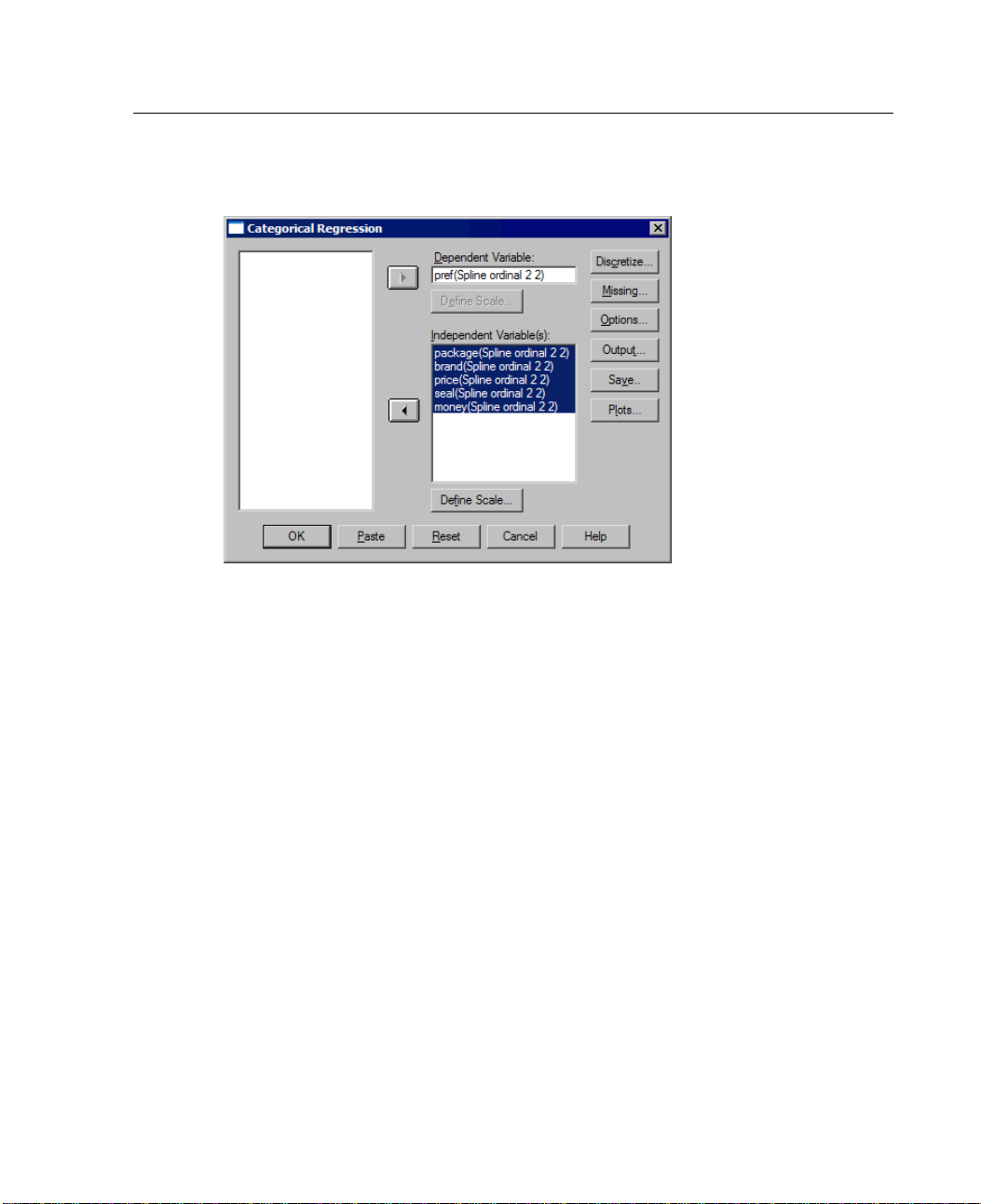
To Obtain a Categorical Regression
E From the menus choose:
Analyze
Regressi
regression analysis.
on
Optimal S
caling...
Page 37
21
Categorical Re
Figure 2-1
Categorical Regression dialog box
E Select the dependent variable and independent variable(s).
E Click OK.
gression (CATREG)
Optionally, change the scaling level for each variable.
Define Scale in Categorical Regression
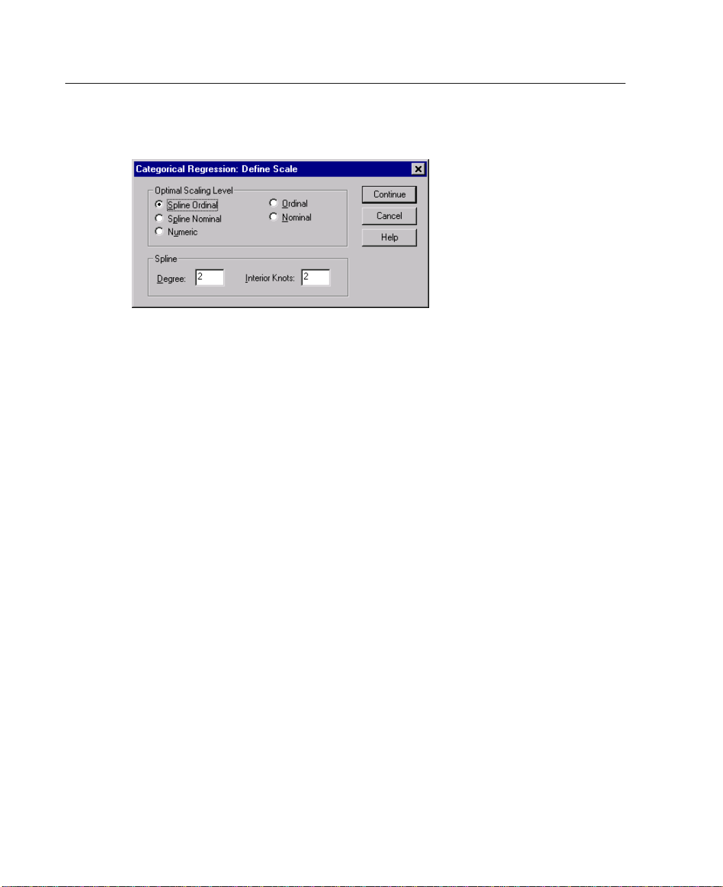
You can set the optimal scaling level for the dependent and independent variables.
By default, they are scaled as second-degree monotonic splines (ordinal) with two
interior knots. Additionally, you can set the weight for analysis variables.
Page 38
22
Chapter 2
Figure 2-2
Define Scale dialog box
Optimal Scaling Level. You can also select the scaling level for quantifying each
variable
Spline Or
.
dinal.
The order of the categories of the observed variable is preserved in
the optimally scaled variable. Category points will be on a straight line (vector)
through the origin. The resulting transformation is a smooth monotonic piecewise
polynomi
al of the chosen degree. The pieces are specified by the user-specified
number and procedure-determined placement of the interior knots.
Spline Nominal. The only information in the observed variable that is preserved in
the optimally scaled variable is the grouping of objects in categories. The order
of the ca
tegories of the observed variable is not preserved. Category points will
be on a straight line (vector) through the origin. The resulting transformation is a
smooth, possibly nonmonotonic, piecewise polynomial of the chosen degree.
The piec
es are specified by the user-specified number and procedure-determined
placement of the interior knots.
Ordinal. The order of the categories of the observed variable is preserved in the
optimally scaled variable. Category points will be on a straight line (vector)
h the origin. The resulting transformation fits better than the spline ordinal
throug
transformation but is less smooth.
Nominal. The only information in the observed variable that is preserved in the
optimally scaled variable is the grouping of objects in categories. The order of
tegories of the observed variable is not preserved. Category points will be
the ca
Page 39

23
Numeric. Ca
Categoric
The Discre
variables. Fractional-value variables are grouped into seven categories (or into the
number of distinct values of the variable if this number is less than seven) with an
approxim
always converted into positive integers by assigning category indicators according
to ascending alphanumeric order. Discretization for string variables applies to
these in
arethenusedintheanalysis.
Categorical Re
on a straight line (vector) through the origin. The resulting transformation fits
better than
The order of the categories and the equal distances between category numbers of
the observed variable are preserved in the optimally scaled variable. Category
points will
at the numeric level, the analysis is analogous to standard principal components
analysis.
the spline nominal transformation but is less smooth.
tegories are treated as ordered and equally spaced (interval level).
be on a straight line (vector) through the origin. When all variables are
gression (CATREG)
al Regression Discretization
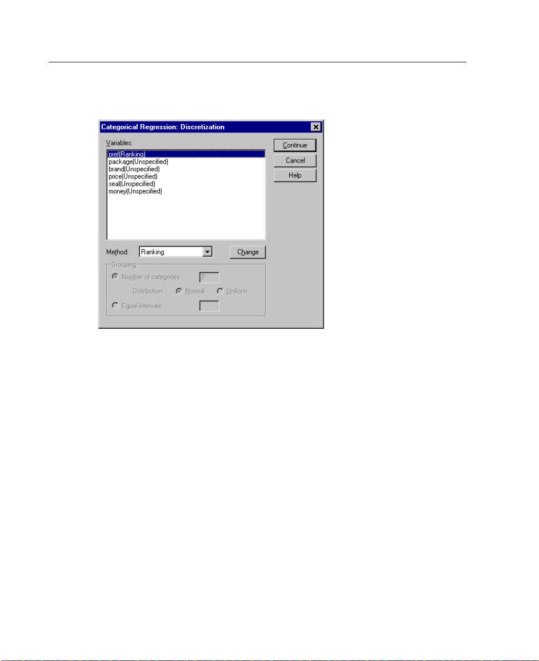
tizationdialogboxallowsyoutoselectamethodofrecodingyour
ately normal distribution unless otherwise specified. String variables are
tegers. Other variables are left alone by default. The discretized variables
Page 40
24
Chapter 2
Figure 2-3
Discretization dialog box
.
Method
Groupi
Rankin
Multip
Choose between grouping, ranking, and multiplying.
ng.
Recode into a specified number of categories or recode by interval.
g.
The variable is discretized by ranking the cases.
lying.
The current values of the variable are standardized, multiplied by 10,
rounded, and have a constant added so that the lowest discretized value is 1.
g.
Groupin
Number
The following options are availablewhen discretizing variables by grouping:
of categories.
Specify a number of categories and whether the values of
the variable should follow an approximately normal or uniform distribution
across those categories.
Equal intervals. Variables are recoded into categories defined by these equally
ntervals. You must specify the length of the intervals.
sized i
Categorical Regression Missing Values
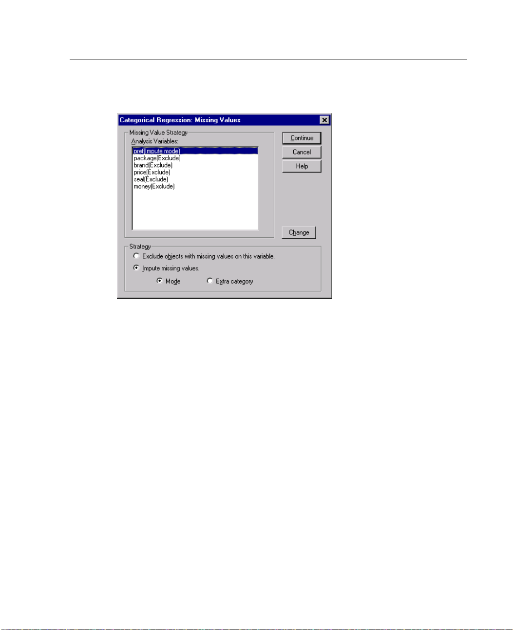
The Missing Values dialog box allows you to choose the strategy for handling missing
in analysis variables and supplementary variables.
values
Page 41
25
Categorical Re
Figure 2-4
Missing Values dialog box
Strategy. Choose to exclude objects with missing values (listwise deletion) or impute
gression (CATREG)
missing values (active treatment).
Exclude objects with missing values on this variable. Objects with missing values
on the selected variable are excluded from the analysis. This strategy is not
available for supplementary variables.
Impute missing values. Objects with missing values on the selected variable have
those values imputed. You can choose the method of imputation. Select
Mode to
replace missing values with the most frequent category. When there are multiple
modes, the one with the smallest category indicator is used. Select
Extra category
to replace missing values with the same quantification of an extra category.
This implies that objects with a missing value on this variable are considered to
belong to the same (extra) category.
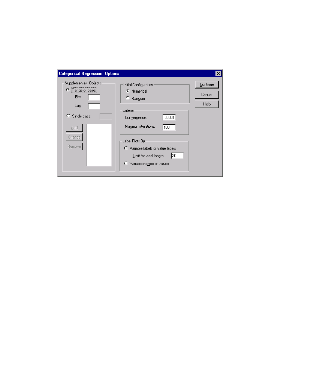
Categorical Regression Options
The Options dialog box allows you to select the initial configuration style, specify
iteration and convergence criteria, select supplementary objects, and set the labeling
of plots.
Page 42
26
Chapter 2
Figure 2-5
Options dialog box
Supplementary Objects. This allows you to specify the objects that you want to treat as
supplem
entary. Simply type the number of a supplementary object and click
Add.
You can not weight supplementary objects (specified weights are ignored).
Initial Configuration. If no variables are treated as nominal, select the Numerical
configu
ration. If at least one variable is treated as nominal, select the
configuration.
Criteria. You can specify the maximum number of iterations that the regression may
ugh in its computations. You can also select a convergence criterion value. The
go thro
regression stops iterating if the difference in total fit between the last two iterations is
less than the convergence value or if the maximum number of iterations is reached.
Label P
lots By.
Allows you to specify whether variables and value labels or variable
names and values will be used in the plots. You can also specify a maximum length
for labels.
Categorical Regression Output
The Output dialog box allows you to select the statistics to display in the output.
Random
Page 43
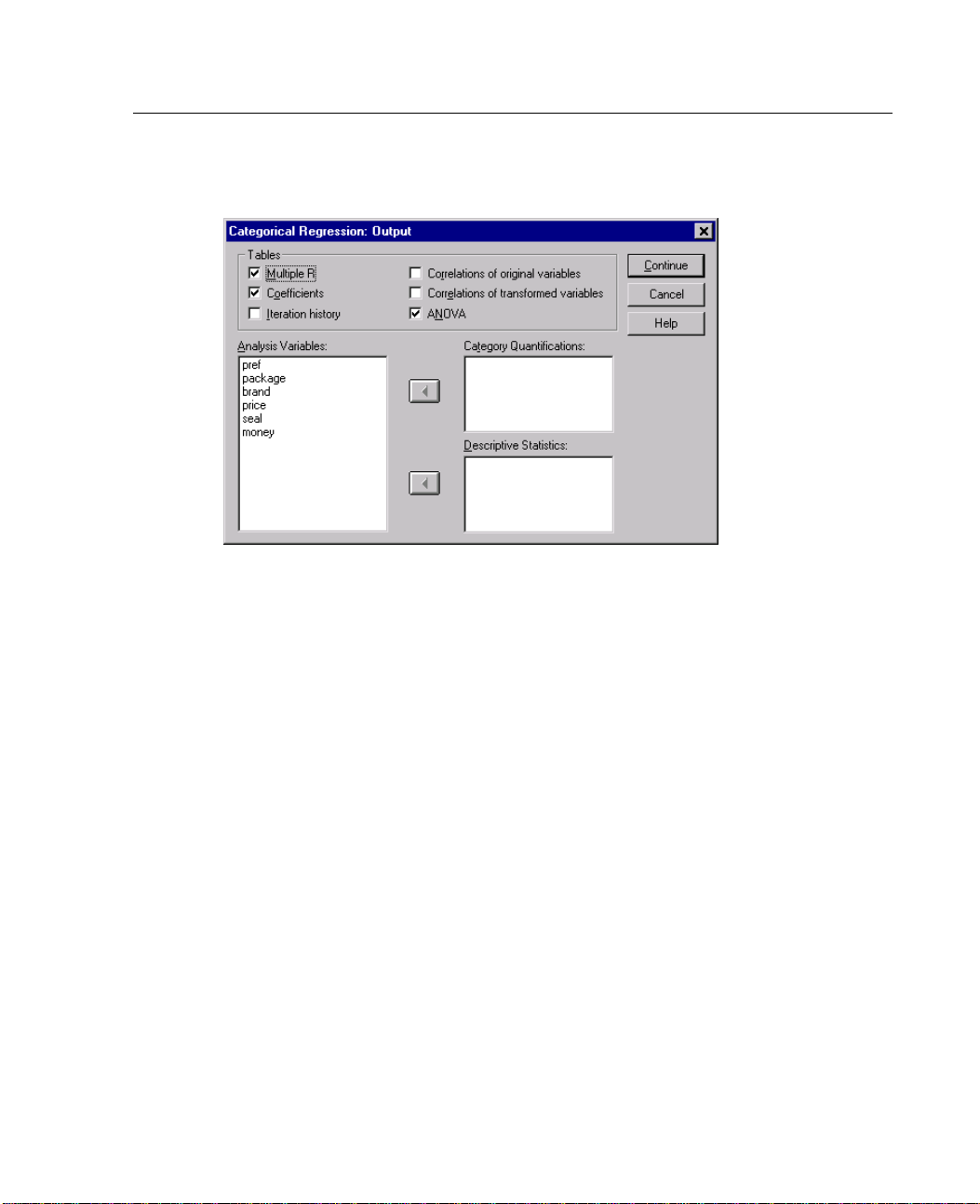
27
Categorical Re
Figure 2-6
Output dialog box
gression (CATREG)
Tables. Produces tables for:
Multiple R. Includes R
2
,adjustedR2, and adjusted R2taking the optimal scaling
into account.
Coefficients. This option givesthree tables: a Coefficientstable that includes betas,
standard error of the betas, t values, and significance; a Coefficients-Optimal
Scaling table with the standard error of the betas taking the optimal scaling
degrees of freedom into account; and a table with the zero-order, part, and partial
correlation, Pratt’s relative importance measure for the transformed predictors,
and the tolerance before and after transformation.
Iteration history. For each iteration, including the starting values for the algorithm,
the multiple R and regression error are shown.TheincreaseinmultipleR is
listed starting from the first iteration.
Correlations of the original variables. A matrix showing the correlations between
the untransformed variables is displayed.
Page 44
28
Chapter 2
Correlations of the transformed variables. A matrix showing the correlations
between the
ANOVA. This
transformed variables is displayed.
option includes regression and residual sums of squares, mean
squares, and F. T wo ANOVA tables are displayed: one with degrees of freedom
for the regression equal to the number of predictor variables and one with degrees
of freedom f
Category Quantifications. Tables showing the transformed values of the selected
or the regression taking the optimal scaling into account.
variables are displayed.
Descriptiv
of the selected variables are displayed.
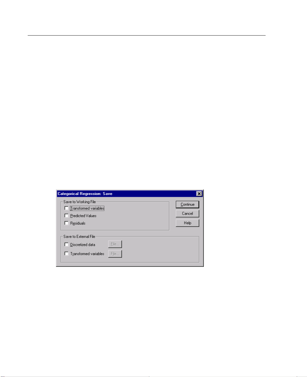
Categoric
The Save di
Figure 2-7
Save dialog box
Save to Working File. You can save the transformed values of the variables,
model-predicted values, and residuals to the working file.
e Statistics.
Tables showing the frequencies, missing values, and modes
al Regression Save
alog box allows you to save results to the working file or an external file.
Save to
External File.
to external files.
You can save the discretized data and transformed variables
Page 45
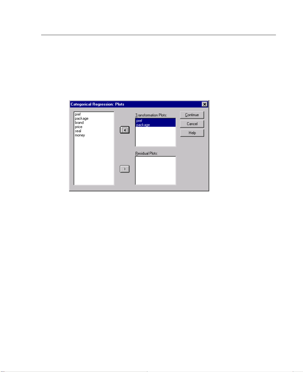
29
Categorical
The Plots di
transformation and residual plots.
Figure 2-8
Plots dialo
Transformation Plots. For each of these variables, the category quantifications are
plotted
horizontal axis but do not affect the computations. These categories are identified by
breaks in the line connecting the quantifications.
Categorical Re
gression (CATREG)
Regression Transformation Plots
alog box allows you to specify the variables that will produce
gbox
against the original category values. Empty categories appear on the
al Plots.
Residu
variable predicted from all predictor variables except the predictor variable
in question) are plotted against category indicators and the optimal category
fications multiplied with beta against category indicators.
quanti
For each of these variables, residuals (computed for the dependent
CATREG Command Additional Features
You can customize your categorical regression if you paste your selections into
ax window and edit the resulting
asynt
language also allows you to:
Specify rootnames for the transformed variables when saving them to the working
data f
ile (with the
SAVE subcommand).
CATREG command syntax. SPSS command
Page 46

Page 47

Chapter
3
Categorical
Components Analysis (CATPCA
This proce
dimensionality of the data. Categorical principal components analysis is also known
by the acronym CATPCA, for categorical principal components analysis.
The goal of
into a smaller set of uncorrelated components that represent most of the information
found in the original variables. The technique is most useful when a large number
of variab
(subjects and units). By reducing the dimensionality, you interpret a few components
rather than a large number of variables.
Standard
numeric variables. On the other hand, the optimal-scaling approach allows variables
to be scaled at different levels. Categorical variables are optimally quantified in the
specifi
can be modeled.
dure simultaneously quantifies categorical variables while reducing the
principal components analysis is to reduce an original set of variables
les prohibits effective interpretation of the relationships between objects
principal components analysis assumes linear relationships between
ed dimensionality. As a result, nonlinear relationships between variables
Principal
)
Example. Categorical principal components analysis could be used to graphically
display
(high, medium, and low), and job satisfaction. You might find that two dimensions
account for a large amount of variance. The first dimension might separate job
catego
from amount of travel. You also might find that high job satisfaction is related to a
medium amount of travel.
Statis
variance accounted for by centroid coordinates, vector coordinates, total per variable
and per dimension, component loadings for vector-quantified variables, category
quant
the relationship between job category, job division, region, amount of travel
ry from region, whereas the second dimension might separate job division
tics and plots.
ifications and coordinates, iteration history, correlations of the transformed
Frequencies, missing values, optimal scaling level, mode,
31
Page 48

32
Chapter 3
variables and eigenvalues of the correlation matrix, correlations of the original
variables and eigenvalues of the correlation matrix, object scores, category plots, joint
category pl
ots, transformation plots, residual plots, projected centroid plots, object
plots, biplots, triplots, and component loadings plots.
Data. String variable values are always converted into positive integers by ascending
alphanumer
ic order. User-defined missing values, system-missing values, and values
less than 1 are considered missing; you can recode or add a constant to variables with
values less than 1 to make them nonmissing.
ns.
Assumptio
The data must contain at least t hree valid cases. The analysis is based
on positive integer data. The discretization option will automatically categorize
a fractional-valued variable by grouping its values into categories with a close to
“normal”
distribution and will automatically convert values of string variables into
positive integers. You can specify other discretization schemes.
Related procedures. Scaling all variables at the numeric level corresponds to standard
principa
l components analysis. Alternate plotting features are available by using
the transformed variables in a standard linear principal components analysis. If all
variables have multiple nominal scaling levels, categorical principal components
s is identical to multiple correspondence analysis. If sets of variables are of
analysi
interest, categorical (nonlinear) canonical correlation analysis should be used.
To Obtai
E From th
Analyze
Data Reduction
Optimal Scaling...
n a Categorica l Principal Components Analysis
e menus choose:
Page 49
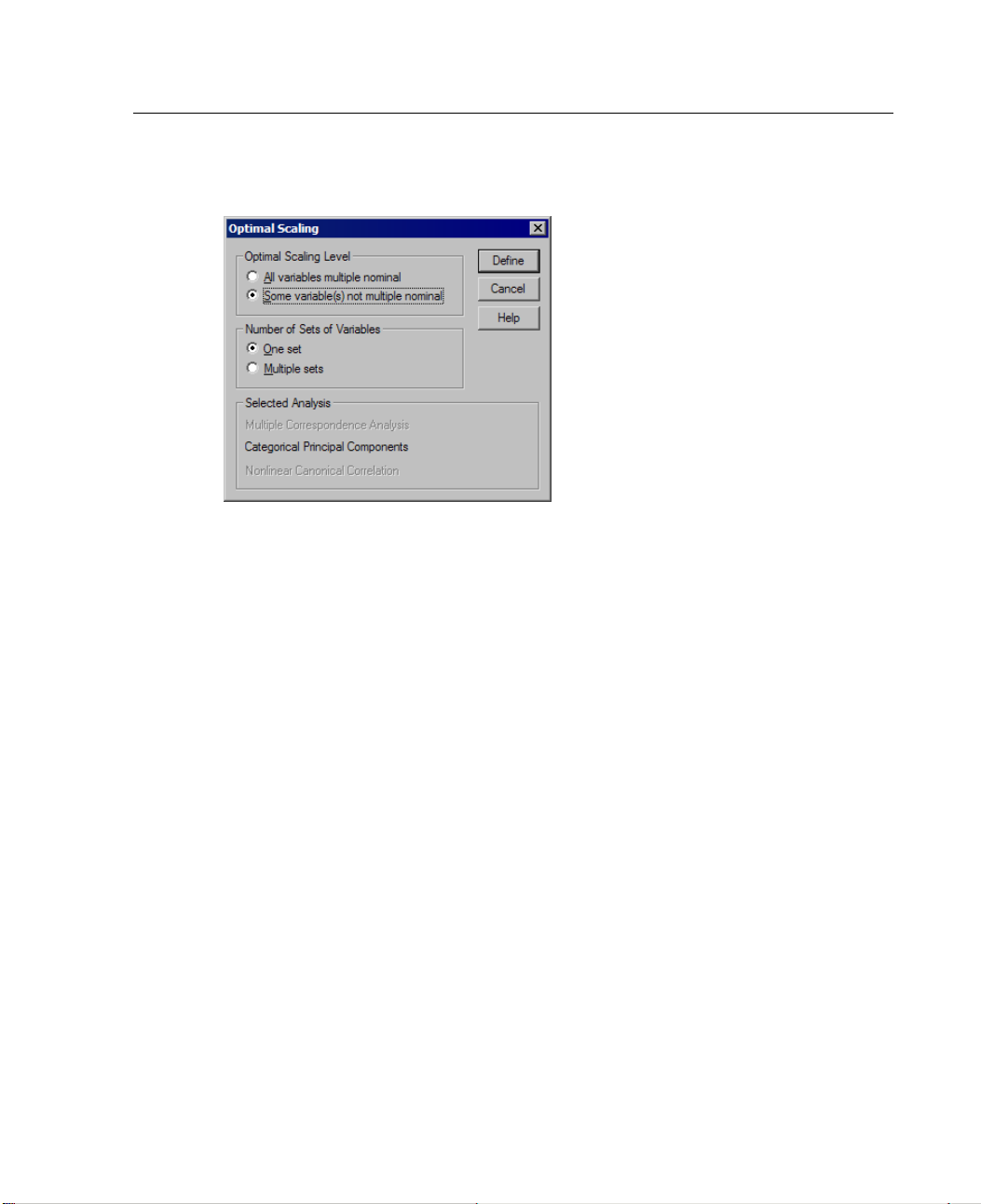
33
Categorical Pr
Figure 3-1
Optimal Scaling dialog box
E Select Some variable(s) not multiple nominal.
E Select One set.
E Click Define.
incipal Components Analysis (CATPCA)
Page 50
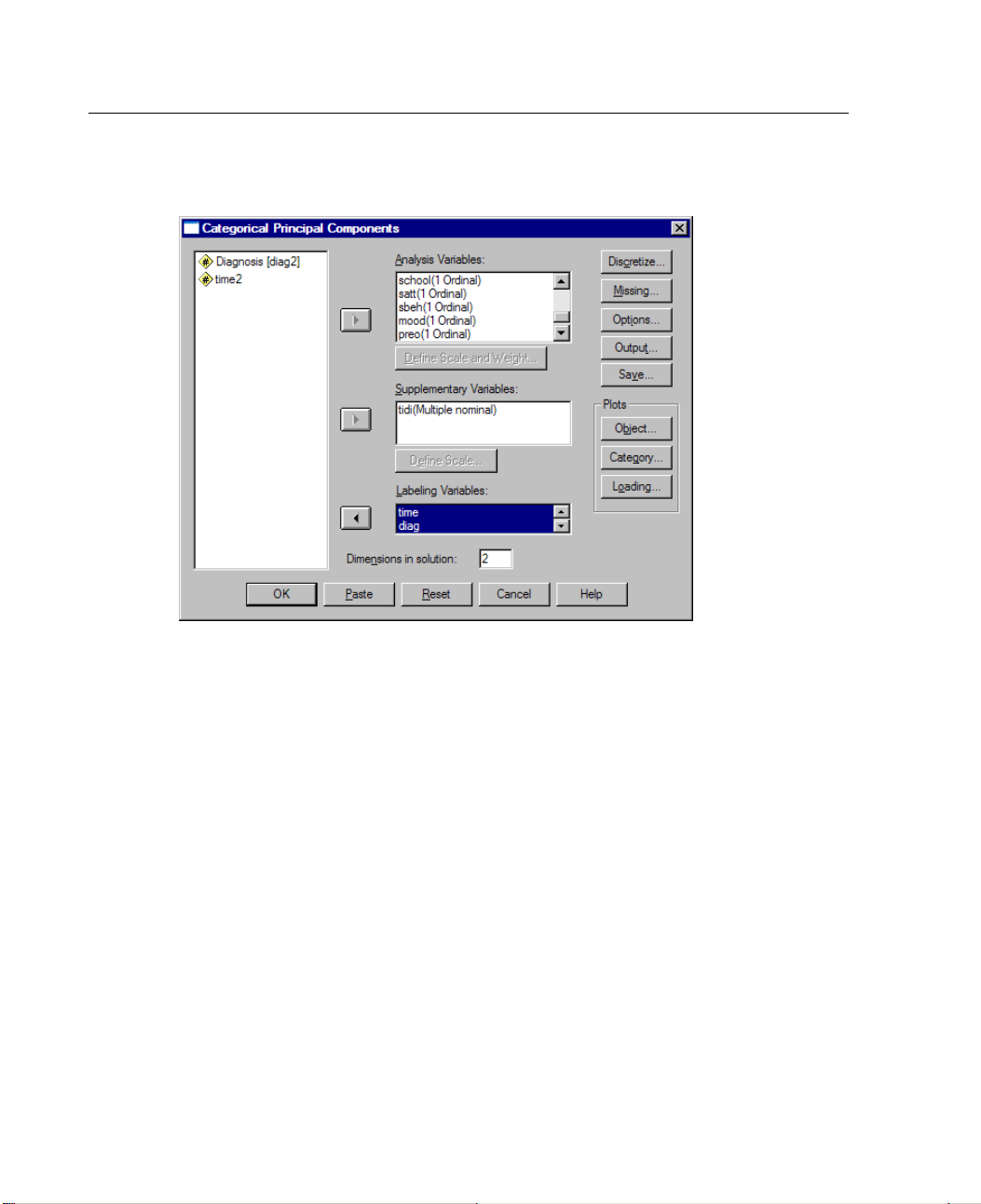
34
Chapter 3
Figure 3-2
Categorical Principal Components dialog box
E Select at least two analysis variables and specify the number of dimensions in the
solution.
E Click OK.
You may optionally specify supplementary variables, which are fitted into the solution
found, or labeling variables for the plots.
Define Scale and Weight in CATPCA
You can set the optimal scaling level for analysis variables and supplementary
variables. By default, they are scaled as second-degree monotonic splines (ordinal)
with two interior knots. Additionally, you can set the weight for analysis variables.
Page 51
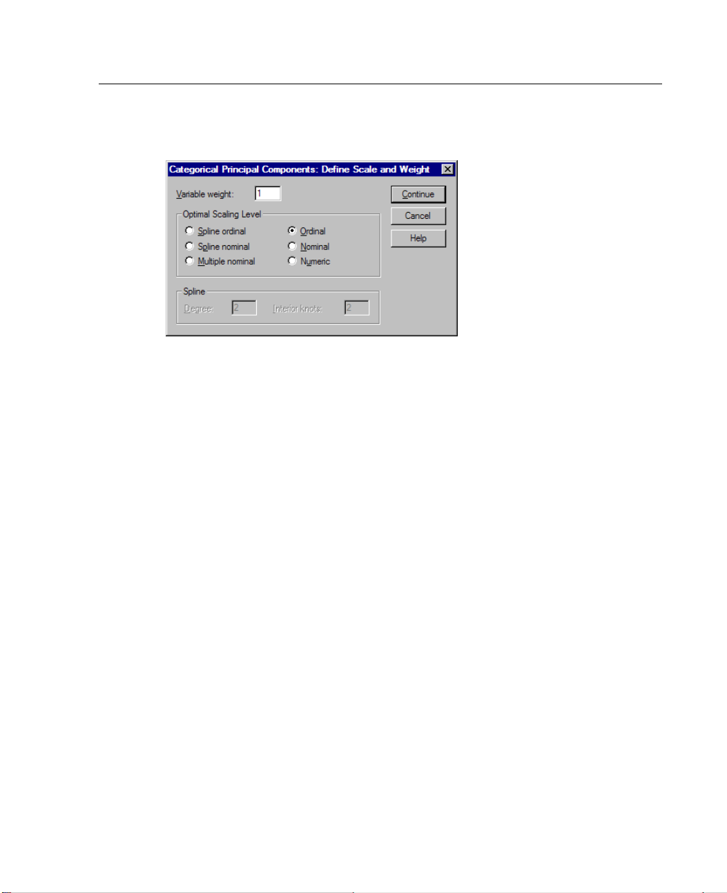
35
Categorical Pr
Figure 3-3
Define Scale a nd Weight dialog box
Variable weight. You can choose to define a weight for each variable. The value
incipal Components Analysis (CATPCA)
specified must be a positive integer. The default value is 1.
Optimal S
caling Level.
You can also select the scaling level to be used to quantify
each variable.
Spline ordinal. The order of the categories of the observed variable is preserved in
the optim
ally scaled variable. Category points will be on a straight line (vector)
through the origin. The resulting transformation is a smooth monotonic piecewise
polynomial of the chosen degree. The pieces are specified by the user-specified
number a
Spline
nd procedure-determined placement of the interior knots.
nominal.
The only information in the observed variable that is preserved in
the optimally scaled variable is the grouping of objects in categories. The order
of the categories of the observed variable is not preserved. Category points will
be on a s
traight line (vector) through the origin. The resulting transformation is a
smooth, possibly nonmonotonic, piecewise polynomial of the chosen degree.
The pieces are specified by the user-specified number and procedure-determined
placem
Multi
ent of the interior knots.
ple nominal.
The only information in the observed variable that is preserved
in the optimally scaled variable is the grouping of objects in categories. The order
of the categories of the observed variable is not preserved. Category points will
he centroid of the objects in the particular categories. Multiple indicates
be in t
that different sets of quantifications are obtained for each dimension.
Page 52

36
Chapter 3
Ordinal. The order of the categories of the observed variable is preserved in the
optimally s
through the origin. The resulting transformation fits better than the spline ordinal
transformation but is less smooth.
Nominal. The only information in the observed variable that is preserved in the
optimally s
the categories of the observed variable is not preserved. Category points will be
on a straight line (vector) through the origin. The resulting transformation fits
better tha
Numeric.
The order of the categories and the equal distances between category numbers of
the observed variable are preserved in the optimally scaled variable. Category
points wi
at the numeric level, the analysis is analogous to standard principal components
analysis.
caled variable. Category points will be on a straight line (vector)
caled variable is the grouping of objects in categories. The order of
n the spline nominal transformation but is less smooth.
Categories are treated as ordered and equally spaced (interval level).
ll be on a straight line (vector) through the origin. When all variables are
Categori
cal Principal Components Analysis Discretization
The Disc
variables. Fractional-valued variables are grouped into seven categories (or into the
number of distinct values of the variable if this number is less than seven) with an
approxi
always converted into positive integers by assigning category indicators according
to ascending alphanumeric order. Discretization for string variables applies to
these i
arethenusedintheanalysis.
retizationdialogboxallowsyoutoselectamethodofrecodingyour
mately normal distribution, unless specified otherwise. String variables are
ntegers. Other variables are left alone by default. The discretized variables
Page 53
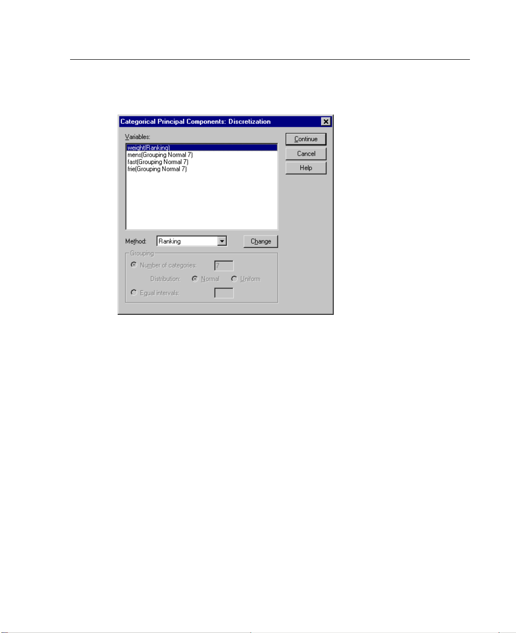
37
incipal Components Analysis (CATPCA)
Figure 3-4
Discretization dialog box
.
Method
Groupi
Rankin
Multip
Choose between grouping, ranking, and multiplying.
ng.
Recode into a specified number of categories or recode by interval.
g.
The variable is discretized by ranking the cases.
lying.
The current values of the variable are standardized, multiplied by 10,
Categorical Pr
rounded, and have a constant added such that the lowest discretized value is 1.
g.
Groupin
The following options are available when you are discretizing variables
by grouping:
Number of categories. Specify a number of categories and whether the values of
iable should follow an approximately normal or uniform distribution
the var
across those categories.
Equal intervals. Variables are recoded into categories defined by these equally
sized intervals. You must specify the length of the intervals.
Page 54
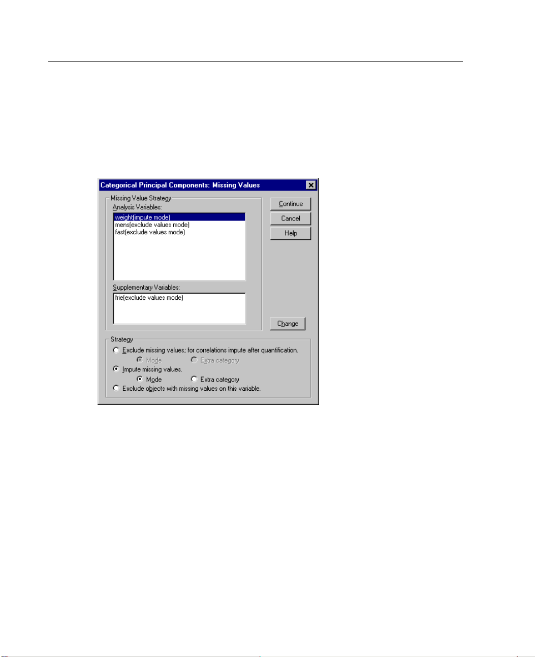
38
Chapter 3
Categorical
The Missing
values in analysis variables and supplementary variables.
Figure 3-5
Missing Val
Principal Components Analysis Missing Values
Values dialog box allows you to choose the strategy for handling missing
ues dialog box
g Value Strategy.
Missin
Choose to exclude missing values (passive treatment), impute
missing values (active treatment), or exclude objects with missing values (listwise
deletion).
Exclude missing values; for correlations impute after quantification. Objects with
missing values on the selected variable do not contribute to the analysis for this
ble. If all variables are given passive treatment, then objects with missing
varia
values on all variables are treated as supplementary. If correlations are specified
in the Output dialog box, then (after analysis) missing values are imputed with the
frequent category,or mode, of the variable for the correlations of the original
most
variables. For the correlations of the optimally scaled variables, you can choose
the method of imputation. Select
ptimally scaled variable. Select
the o
Mode to replace missing values with the mode of
Extra category to replace missing values with
Page 55

39
Categori
Categorical Pr
incipal Components Analysis (CATPCA)
the quantification of an extra category. This implies that objects with a missing
value on thi
Impute miss
those values imputed. You can choose the method of imputation. Select
s variable are considered to belong to the same (extra) category.
ing values.
Objects with missing values on the selected variable have
Mode to
replace missing values with the most frequent category. When there are multiple
modes, the o
ne with the smallest category indicator is used. Select
Extra category
to replace missing values with the same quantification of an extra category.
This implies that objects with a missing value on this variable are considered to
belong to t
Exclude o
he same (extra) category.
bjects with missing values on this variable.
Objects with missing values
on the selected variable are excluded from the analysis. This strategy is not
available for supplementary variables.
cal Principal Components Analysis Options
The Optio
and convergence criteria, select a normalization method, choose the method for
labeling plots, and specify supplementary objects.
ns dialog box allows you to select the initial configuration, specify iteration
Page 56
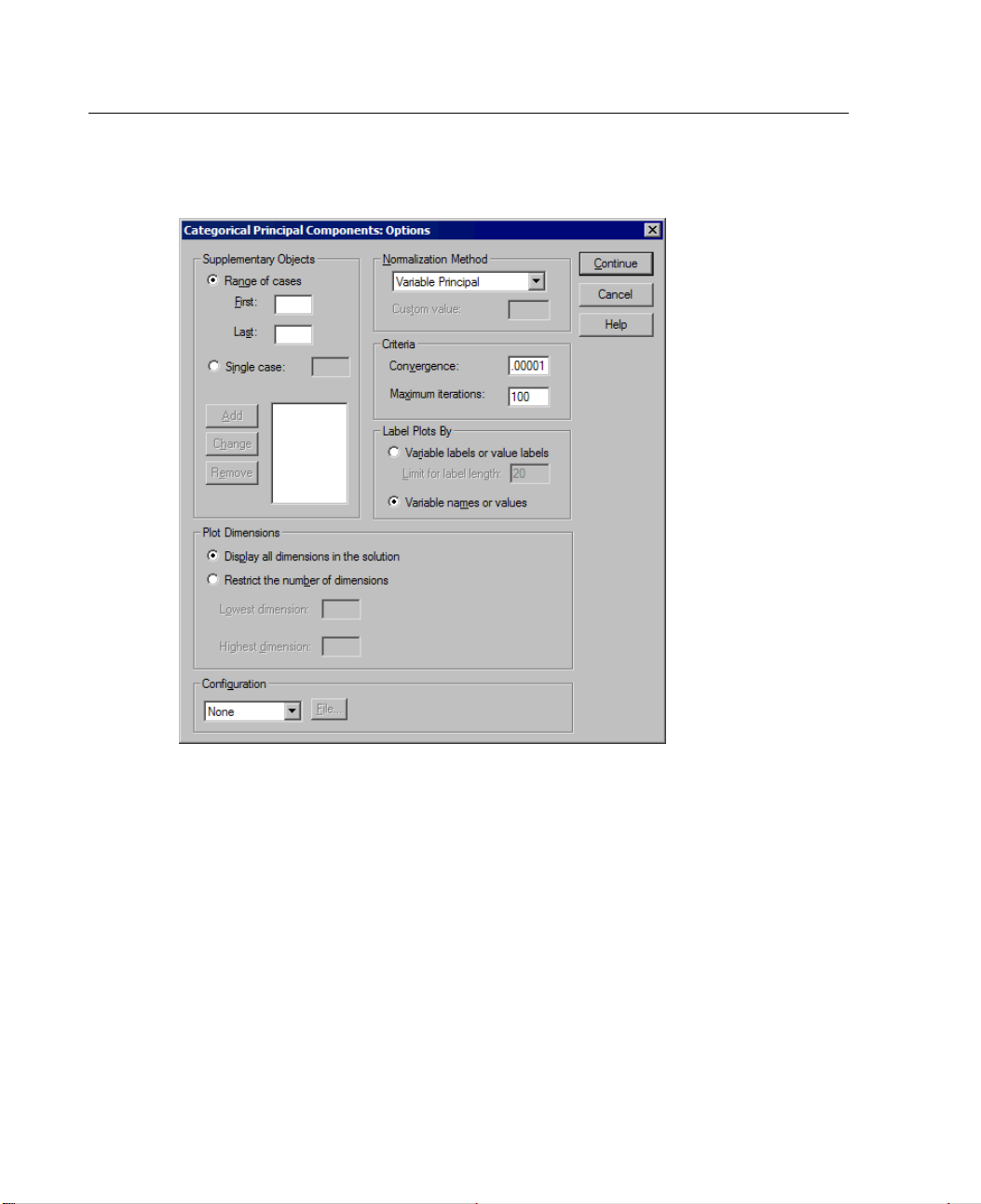
40
Chapter 3
Figure 3-6
Options dialog box
Supplementary Objects. Specify the case number of the object, or the first and last case
numbers of a range of objects, that you want to make supplementary and then click
Add. Continue until you have specified all of your supplementary objects. If an object
is specified as supplementary, then case weights are ignored for that object.
Normalization Method. You can specify one of five options for normalizing the
object scores and the variables. Only one normalization method can be used in
a given analysis.
Variable Principal. This option optimizes the association between variables. The
coordinates of the variables in the object space are the component loadings
(correlations with principal components, such as dimensions and object scores).
This is useful when you are primarily interested in the correlation between the
variables.
Page 57

41
Categorical Pr
Object Principal. This option optimizes distances between objects. This is useful
when you are
primarily interested in differences or similarities between the
incipal Components Analysis (CATPCA)
objects.
Symmetrical. Use this normalization option if you are primarily interested in the
relation between objects and variables.
Independent. Use this normalization option if you want to examine distances
between obj
Custom. Yo
ects and correlations between variables separately.
u can specify any real value in the closed interval [–1, 1]. A value of 1
is equal to the Object Principal method, a value of 0 is equal to the Symmetrical
method, and a value of –1 is equal to the Variable Principal method. By
specifyin
g a value greater than –1 and less than 1, you can spread the eigenvalue
over both objects and variables. This method is useful for making a tailor-made
biplot or triplot.
Criteria. You can specify the maximum number of iterations the procedure can go
through i
n its computations. You can also select a convergence criterion value. The
algorithm stops iterating if the difference in total fit between the last two iterations is
less than the convergence value or if the maximum number of iterations is reached.
ts By.
Label Plo
Allows you to specify whether variables and value labels or variable
names and values will be used in the plots. You can also specify a maximum length
for labels.
Plot Dime
Display
nsions.
Allows you to control the dimensions displayed in the output.
all dimensions in the solution.
All dimensions in the solution are displayed
in a scatterplot matrix.
Restrict the number of dimensions. The displayed dimensions are restricted to
plotted pairs. If you restrict the dimensions, you must select the lowest and
highest
dimensions to be plotted. The lowest dimension can range from 1 to the
number of dimensions in the solution minus 1 and is plotted against higher
dimensions. The highest dimension value can range from 2 to the number of
dimens
ions in the solution and indicates the highest dimension to be used
in plotting the dimension pairs. This specification applies to all requested
multidimensional plots.
Page 58

42
Chapter 3
Configuration. You can read data from a file containing the coordinates of a
configuration. The first variable in the file should contain the coordinates for the
first dimen
sion, the second variable should contain the coordinates for the second
dimension, and so on.
Initial. The configuration in the file specified will be used as the starting point
of the analy
Fixed. The
sis.
configuration in the file specified will be used to fit in the variables.
The variables that are fitted in must be selected as analysis variables, but because
the configuration is fixed, they are treated as supplementary variables (so they do
not need to
be selected as supplementary variables).
Categorical Principal Components Analysis Output
The Output dialog box allows you to produce tables for object scores, component
loadings
variance accounted for per variable and per dimension, category quantifications for
selected variables, and descriptive statistics for selected variables.
, iteration history, correlations of original and transformed variables, the
Page 59
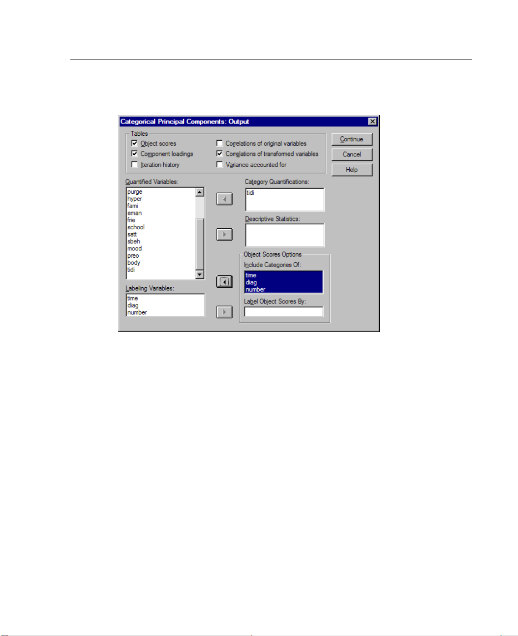
43
Categorical Pr
Figure 3-7
Output dialog box
incipal Components Analysis (CATPCA)
Object scores. Displays the object scores and has the following options:
Include Categories Of. Displays the category indicators of the analysis variables
selected.
Label Object Scores By. From the list of variables specified as labeling variables,
you can select one to label the objects.
Component loadings. Displays the component loadings for all variables that were not
given multiple nominal scaling levels.
Iteration history. For each iteration, the variance accounted for, loss, and increase
in variance accounted for are shown.
Correlations of original variables. Shows the correlation matrix of the original variables
and the eigenvalues of that matrix.
Correlations of transformed variables. Shows the correlation matrix of the transformed
(optimally scaled) variables and the eigenvalues of that matrix.
Page 60
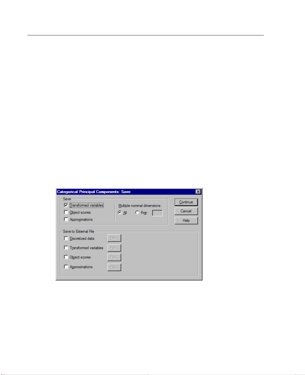
44
Chapter 3
Variance accounted for. Displays the amount of variance accounted for by centroid
coordinates, vector coordinates, and total (centroid and vector coordinates combined)
per variabl
e and per dimension.
Category Qu
antifications.
Gives the category quantifications and coordinates for each
dimension of the variable(s) selected.
Descriptive Statistics. Displays frequencies, number of missing values, and mode of
the variable(s) selected.
Categorical Principal Components Analysis Save
The Save dialog box allows you to add the transformed variables, object scores, and
approximations to the working data file or as new variables in external files and save
the discre
Figure 3-8
Save dialog box
tized data as new variables in an external data file.
Save. Save selections to the working data file. If any variable has been given the
multiple nominal scaling level, the number of dimensions to be saved must be
specified.
Save to External File. Save selections to a new external file. Specify a filename for
each selected option by clicking
File. Each file specified must have a different name.
Page 61
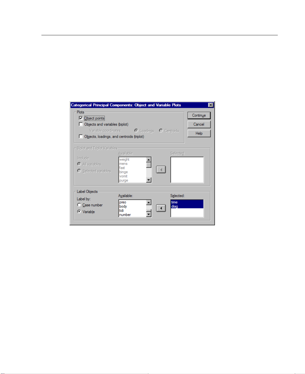
45
Categorical
The Object a
desired and the variables for which plots will be produced.
Figure 3-9
Object and V
Categorical Pr
incipal Components Analysis (CATPCA)
Principal Components Analysis Object Plots
nd Variable Plots dialog box allows you to specify the types of plots
ariable Plots dialog box
Object points. A plot of the object points is displayed.
s and variables (biplot).
Object
The object points are plotted with your choice of the
variable coordinates—component loadings or variable centroids.
Objects, loadings, and centroids (triplot). The object points are plotted with the
ids of multiple nominal-scaling-level variables and the component loadings
centro
of other variables.
Biplot and Triplot Variables. You can choose to use all variables for the biplots and
ots or select a subset.
tripl
Page 62
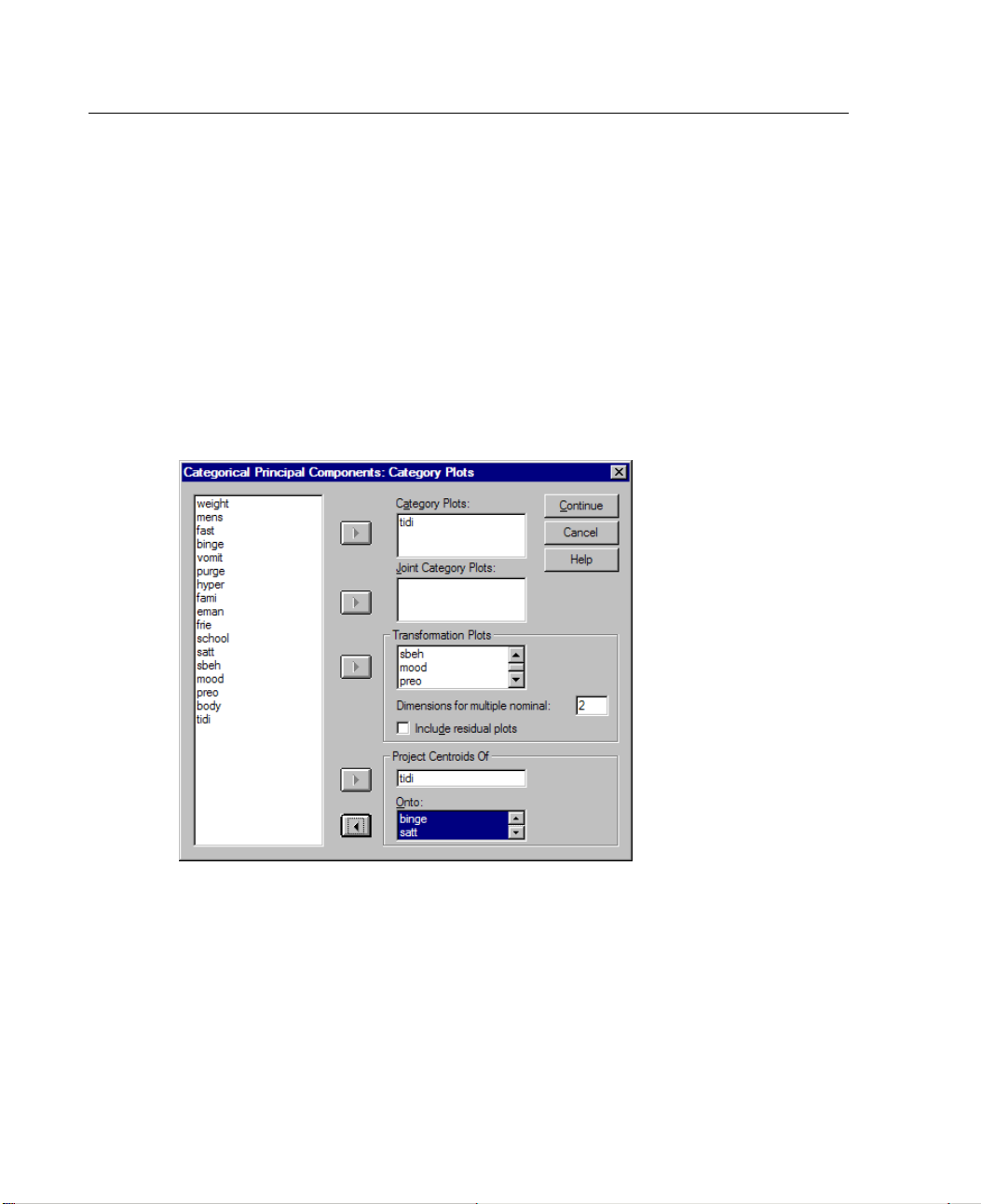
46
Chapter 3
Label Objects. You can choose to have objects labeled with the categories of selected
variables ( you may choose category indicator values or value labels in the Options
dialog box)
or with their case numbers. One plot is produced per variable if
Variable is
selected.
Categorica
The Catego
variables for which plots will be produced.
Figure 3-1
Category P
l Principal Components Analysis Category Plots
ry Plots dialog box allows you to specify the types of plots desired and the
0
lots dialog box
Category Plots. For each variable selected, a plot of the centroid and vector coordinates
is plotted. For variables with multiple nominal scaling levels, categories are in the
oids of the objects in the particular categories. For all other scaling levels,
centr
categories are on a vector through the origin.
Joint Category Plots. This is a single plot of the centroid and vector coordinates of
selected variable.
each
Page 63
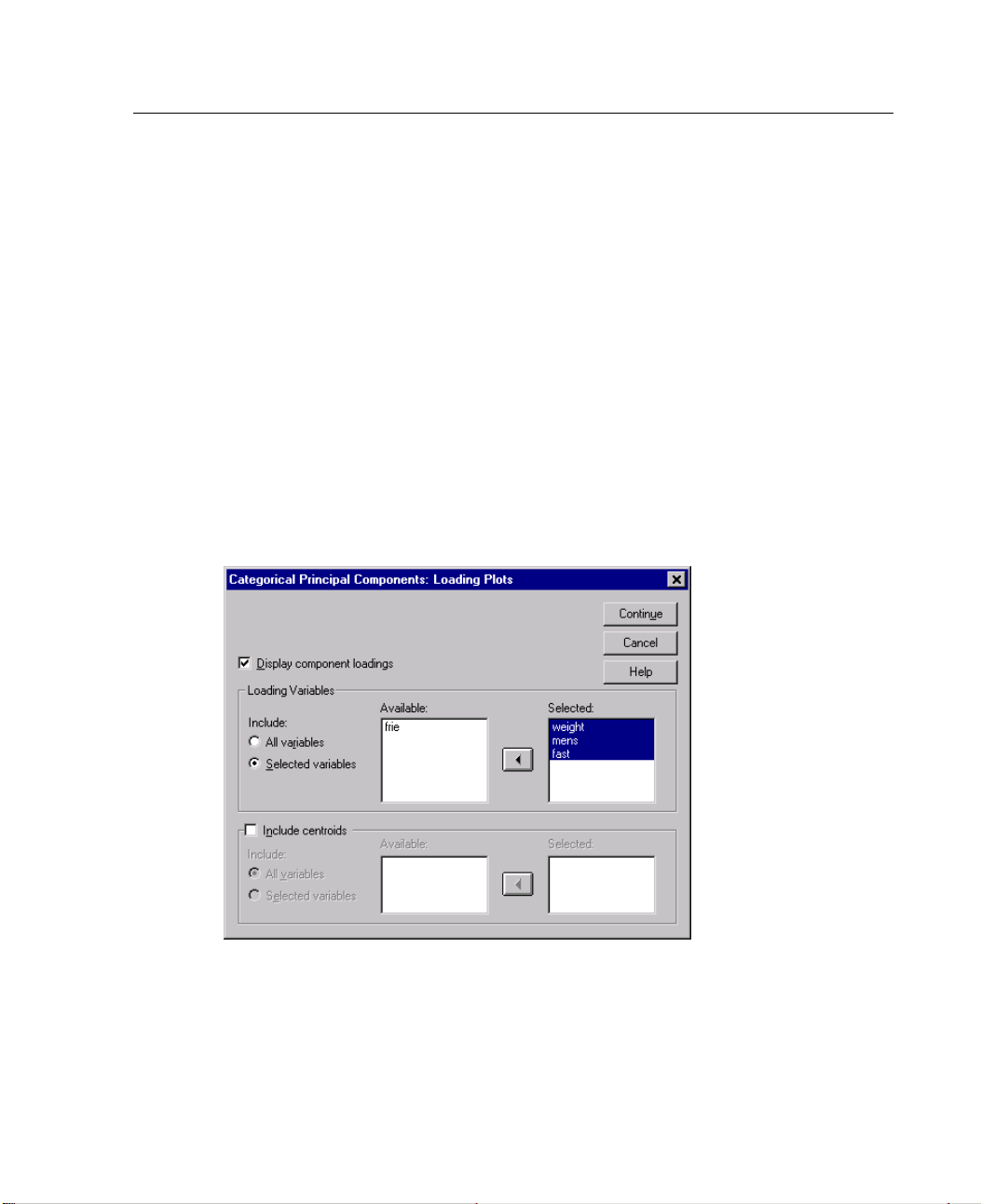
47
Categorical Pr
Transformation Plots. Displays a plot of the optimal category quantifications versus the
incipal Components Analysis (CATPCA)
category indicators. You can specify the numberofdimensionsdesiredforvariables
with multip
le nominal scaling levels; one plot will be generated for each dimension.
You can also choose to display residual plots for each variable selected.
Project Centroids Of. You may choose a variable and project its centroids onto selected
variables.
Variables with multiple nominal scaling levels cannot be selected to project
on. When this plot is requested, a table with the coordinates of the projected centroids
is also displayed.
Categorical Principal Components Analysis Loading Plots
The Loading Plots dialog box allows you to specify the variables which will be
included in the plot, and whether or not to include centroids in the plot.
Figure 3-11
Loading Plots dialog box
Display component loadings. If selected, a plot of the component loadings is displayed.
Loading Variables. You can choose to use all variables for the component loadings
r select a subset.
plot o
Page 64

48
Chapter 3
Include centroids. Variables with multiple nominal scaling levels do not have
component loadings, but you may choose to include the centroids of those variables
in the plot.
You can choose to use all multiple nominal variables or select a subset.
CATPCA Command Additional Features
You can customize your categorical principal components analysis if you paste your
selection
SPSS command language also allows you to:
Specify rootnames for the transformed variables, object scores, and
Specify a maximum length for labels for each plot separately (with the PLOT
Specify a separate variable list for residual plots (with the PLOT subcommand).
s into a syntax window and edit the resulting
approxima
tionswhensavingthemtotheworkingdatafile(withthe
subcommand).
subcommand).
CATPCA command syntax.
SAVE
Page 65

Chapter
4
Nonlinear Ca
nonical
Correlation Analysis (OVERALS)
Nonlinear
Canonical Correlation Analysis
Nonlinea
correlation analysis with optimal scaling. The purpose of this procedure is to
determine how similar sets of categorical variables are to one another. Nonlinear
canonica
where the second set does not contain a single response variable, but multiple ones.
The goal
among two sets of numerical variables in a low dimensional space. Initially, the
variables in each set are linearly combined such that the linear combinations have
amaxima
are determined that are uncorrelated with the previous combinations and that have
the largest correlation possible.
First, OVERALS allows more than two sets of variables. Second, variables can be
scaled as either nominal, ordinal, or numerical. As a result, nonlinear relationships
betwee
between the variable sets, the sets are compared to an unknown compromise set
defined by the object scores.
r canonical correlation analysis corresponds to categorical canonical
l correlation analysis is also known by the acronym OVERALS.
Standard canonical correlation analysis is an extension of multiple regression,
is to explain as much as possible of the variance in the relationships
l correlation. Given these combinations, subsequent linear combinations
The opt
imal scaling approach expands the standard analysis in three crucial ways.
n variables can be analyzed. Finally, instead of maximizing correlations
le.
Examp
used to graphically display the relationship between one set of variables containing
job category and years of education and another set of variables containing region of
resi
Categorical canonical correlation analysis with optimal scaling could be
dence and gender. You might find that years of education and region of residence
49
Page 66

50
Chapter 4
discriminate better than the remaining variables. You might also find that years of
education discriminates best on the first dimension.
Statistics
and plots.
Frequencies, centroids, iteration history, object scores, category
quantifications, weights, component loadings, single and multiple fit, object scores
plots, category coordinates plots, component loadings plots, category centroids plots,
transforma
Data. Use integers to code categorical variables (nominal or ordinal scaling level). To
tion plots.
minimize output, use consecutive integers beginning with 1 to code each variable.
Variables
scaled at the numerical level should not be recoded to consecutive integers.
To minimize output, for each variable scaled at the numerical level, subtract the
smallest observed value from every value and add 1. Fractional values are truncated
after the
Assumptions. Variables can be classified into two or more sets. Variables in the
decimal.
analysis are scaled as multiple nominal, single nominal, ordinal, or numerical. The
maximum n
umber of dimensions used in the procedure depends on the optimal
scaling level of the variables. If all variables are specified as ordinal, single nominal,
or numerical, the maximum number of dimensions is the minimum of the number of
observa
tions minus 1 and the total number of variables. However, if only two sets of
variables are defined, the maximum number of dimensions is the number of variables
in the smaller set. If some variables are multiple nominal, the maximum number of
dimens
ions is the total number of multiple nominal categories plus the number of
nonmultiple nominal variables minus the number of multiple nominal variables. For
example, if the analysis involves five variables, one of which is multiple nominal with
tegories, the maximum number of dimensions is (4 + 4 – 1), or 7. If you
four ca
specify a number greater than the maximum, the maximum value is used.
Related procedures. If each set contains one variable, nonlinear canonical correlation
sis is equivalent to principal components analysis with optimal scaling. If
analy
each of these variables is multiple nominal, the analysis corresponds to multiple
correspondence analysis. If two sets of variables are involved and one of the sets
ins only one variable, the analysis is identical to categorical regression with
conta
optimal scaling.
Page 67
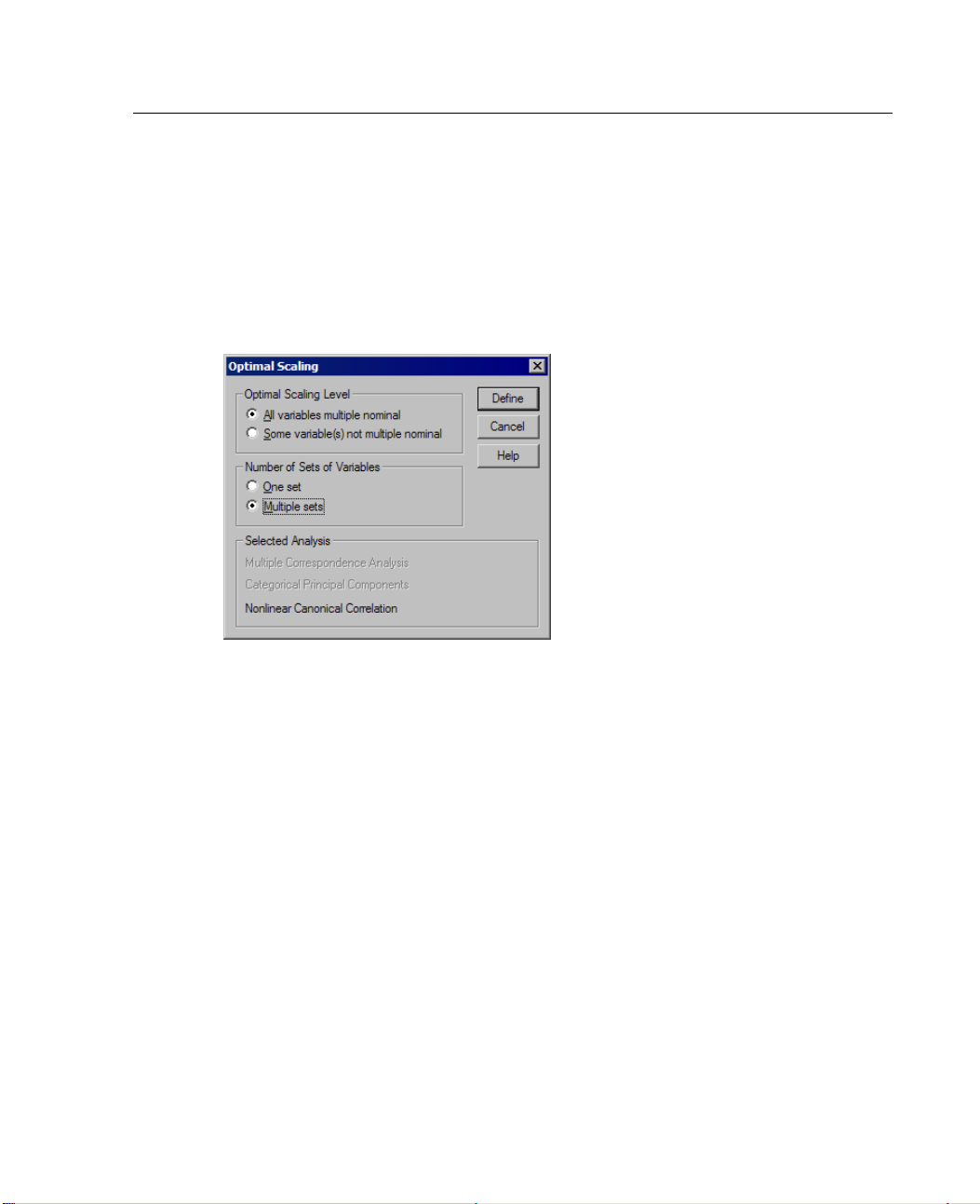
51
Nonlinear Cano
To Obtain a Nonlinea r Canonical Correlation Analysis
E From the menus choose:
Analyze
Data Reduction
Optimal Scaling...
Figure 4-1
Optimal Scaling dialog box
nical Correlation Analysis (OVERALS)
E Select either All variables multiple nominal or Some variable(s) not multiple nominal.
E Select Multiple sets.
E Click Define.
Page 68
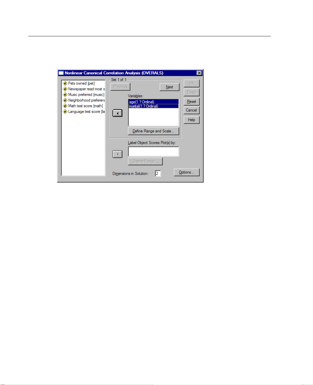
52
Chapter 4
Figure 4-2
Nonlinear Canonical Correlation Analysis (OVERALS) dialog box
E Define at least two sets of variables. Select the variable(s) that you want to include in
the first set. To move to the next set, click Next, and select the variables that you want
to include in the second set. You can add additional sets as desired. Click
Previous to
return to the previously defined variable set.
E Define the value range and measurement scale (optimal scaling level) for each
selected variable.
E Click OK.
Optionally, you can:
Select one or more variables to provide point labels for object scores plots. Each
variable produces a separate plot, with the points labeled by the values of that
variable. You must define a range for each of these plot label variables. Using the
dialog box, a single variable cannot be used both in the analysis and as a labeling
variable. If labeling the object scores plot with a variable used in the analysis
is desired, use the Compute facility on the Transform menu to create a copy of
Page 69
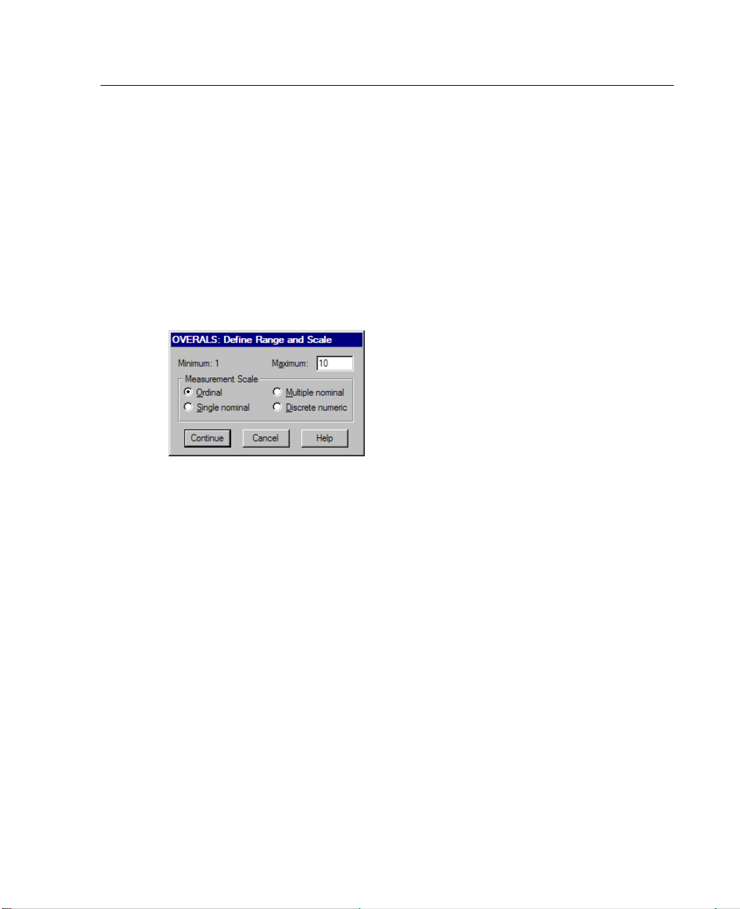
53
that variable. Use the new variable to label the plot. Alternatively, command
syntax can b
Specify the
eused.
number of dimensions you want in the solution. In general, choose as
few dimensions as needed to explainmost of the variation. If the analysis involves
more than two dimensions, SPSS produces three-dimensional plots of the first
three dimen
sions. Other dimensions can be displayed by editing the chart.
Define Range and Scale
Figure 4-3
Define Range and Scale dialog box
You must define a range for each variable. The maximum value specified must be an
integer. Fractional data values are truncated in the analysis. A category value that is
outside
Automatic Recode facility on the Transform menu to create consecutive categories
beginning with 1 for variables treated as nominal or ordinal. Recoding to consecutive
intege
output for variables treated as numerical, for each variable, subtract the minimum
value from every value and add 1.
of the specified range is ignored in the analysis. To minimize output, use the
rs is not recommended for variables scaled at the numerical level. To minimize
Nonlinear Cano
nical Correlation Analysis (OVERALS)
You mus
Ordin
t also select the scaling to be used to quantify each variable.
al.
The order of the categories of the observed variable is preserved in
the quantified variable.
Single nominal. In the quantified variable, objects in the same category receive
thesamescore.
Multiple nominal. The quantifications can be different for each dimension.
Discrete numeric. Categories are treated as ordered and equally spaced. The
ences between category numbers and the order of the categories of the
differ
observed variable are preserved in the quantified variable.
Page 70
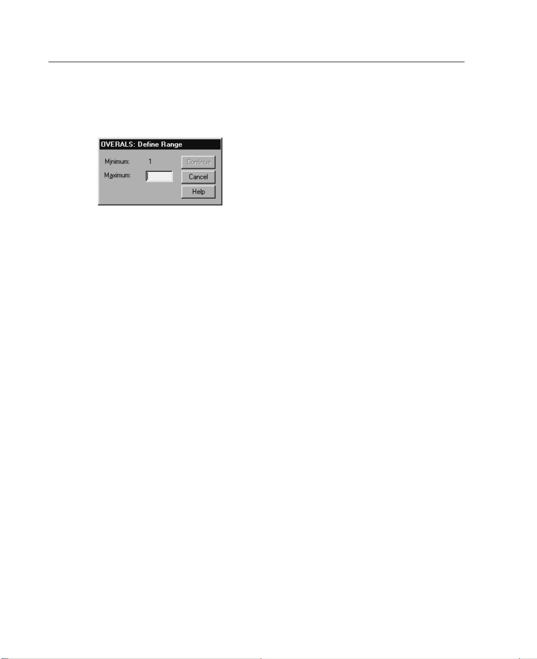
54
Chapter 4
Define Range
Figure 4-4
Define Range dialog box
You must define a range for each variable. The maximum value specified must be an
integer. Fractional data values are truncated in the analysis. A category value that
is outsid
use the Automatic Recode facility on the Transform menu to create consecutive
categories beginning with 1.
You must a
plots. However, labels for categories with data values outside of the defined range
for the variable do appear on the plots.
e of the specified range is ignored in the analysis. To minimize output,
lso define a range for each variable used to label the object scores
Nonlinear Canonical Correlation Analysis Options
The Options dialog box allows you to select optional statistics and plots, save object
scores as new variables in the working data file, specify iteration and convergence
a, and specify an initial configuration for the analysis.
criteri
Page 71
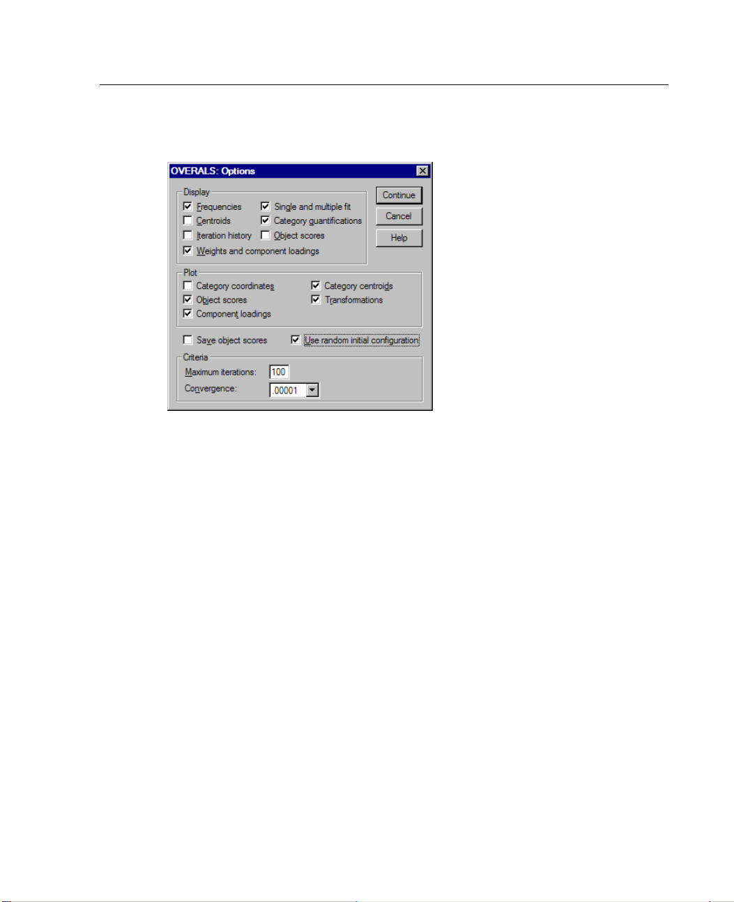
55
Nonlinear Cano
Figure 4-5
Options dialog box
nical Correlation Analysis (OVERALS)
Display. Available statistics include marginal frequencies (counts), centroids, iteration
history, weights and component loadings, category quantifications, object scores, and
single and multiple fit statistics.
Centroids. Category quantifications, and the projected and the actual averages of
the object scores for the objects (cases) included in each set for those belonging
to the same category of the variable.
Weights and Component Loadings. The regression coefficients in each dimension
for every quantified variable in a set, where the object scores are regressed on the
quantified variables, and the projection of the quantified variable in the o bject
space. Provides an indication of the contribution each variable makes to the
dimension within each set.
Single and Mul tiple Fit. Measures of goodness of fit of the single- and
multiple-category coordinates/category quantificationswith respect to the objects.
Category Quantifications. Optimal scale values assigned to the categories of
avariable.
Object Scores. Optimal score assigned to an object (case) in a particular
dimension.
Plot. Yo u can produce plots of category coordinates, object scores, component
loadings, category centroids, and transformations.
Page 72

56
Chapter 4
Save object scores. You can save the object scores as new variables in the working
data file. Object scores are saved for the number of dimensions specified in the
main dialog
Use random initial configuration. A random initial configuration should be used if all
box.
or some of the variables are single nominal. If this option is not selected, a nested
initial con
Criteria. You can specify the maximum number of iterations the nonlinear canonical
figuration is used.
correlation analysis can go through in its computations. You can also select a
convergen
ce criterion value. The analysis stops iterating if the difference in total fit
between the last two iterations is less than the convergence value or if the maximum
number of iterations is reached.
OVERALS Command Additional Features
You can customize your nonlinear canonical correlation analysis if you paste your
selections into a syntax window and edit the resulting OVERALS command syntax.
SPSS comm
Specify
dimensions (using the
Specify the number of value label characters used to label points on the plots
(with the
Designate more than five variables as labeling variables for object scores plots
(with th
Select
plots (with the
Select variables to provide point labels for the quantification score plot (with the
PLOT subcommand).
Specify the number of cases to be included in the analysis, if you do not want to
use all c
Specif
subcommand).
Specify the number of dimensions to be saved, rather than saving all extracted
dimensions (with the
and language also allows you to:
the dimension pairs to be plotted, rather than plotting all extracted
NDIM keywordonthePLOT subcommand).
PLOT subcommand).
PLOT subcommand).
e
variables used in the analysis as labeling variables for the object scores
PLOT subcommand).
ases in the working data file (with the
y rootnames for variables created by saving object scores (with the
SAVE subcommand).
NOBSERVATIONS subcommand).
SAVE
Page 73

57
Nonlinear Cano
Write category quantifications to a matrix file (using the MATRIX subcommand).
Produce low-resolution plots that may be easier to read than the usual
high-resolu
Produce cen
tion plots (using the
troid and transformation plots for specified variables only (with the
SET command).
nical Correlation Analysis (OVERALS)
PLOT subcommand).
Page 74

Page 75

Chapter
5
Corresponde
One of the goals of correspondence analysis is to describe the relationships between
two nominal variables in a correspondence table in a low-dimensional space,
while simultaneously describing the relationships between the categories for each
variable. For each variable, the distances between category points in a plot reflect
the relationships between the categories with similar categories plotted close to each
other. Projecting points for one variable on the vector from the origin to a category
point for the other variable describe the relationship between the variables.
An analysis of contingency tables often includes examining row and column
profiles and testing for independencevia the chi-square statistic. However, the number
of profiles can be quite large, and the chi-square test does not reveal the dependence
structure. The Crosstabs procedure offers several measures of association and tests of
association but cannot graphically represent any relationships between the variables.
Factor analysis is a standard technique for describing relationships between
variables in a low-dimensional space. However, factor analysis requires interval
data, and the number of observations should be five times the number of variables.
Correspondence analysis, on the other hand, assumes nominal variables and can
describe the relationships between categories of each variable, as well as the
relationship between the variables. In addition, correspondence analysis can be used
to analyze any table of positive correspondence measures.
nce Analysis
Example. Correspondence analysis could be used to graphically display the
relationship between staff category and smoking habits. You might find that with
regard to smoking, junior managers differ from secretaries, but secretaries do not
differ from senior managers. You might also find that heavy smoking is associated
with junior managers, whereas light smoking is associated with secretaries.
59
Page 76

60
Chapter 5
Statistics and plots . Correspondence measures, row and column profiles, singular
values, row and column scores, inertia, mass, row and column score confidence
statistics
, singular value confidence statistics, transformation plots, row point plots,
column point plots, and biplots.
Data. Categorical variables to be analyzed are scaled nominally. For aggregated data
or for a corr
espondence measure other than frequencies, use a weighting variable with
positive similarity values. Alternatively, for table data, use syntax to read the t able.
Assumptions. The maximum number of dimensions used in the procedure depends
on the numb
er of active rows and column categories and the number of equality
constraints. If no equality constraints are used and all categories are active, the
maximum dimensionality is one fewer than the number of categories for the variable
with the f
ewest categories. For example, if one variable has five categories and
the other has four, the maximum number of dimensions is three. Supplementary
categories are not active. For example, if one variable has five categories, two of
which are
supplementary, and the other variable has four categories, the maximum
number of dimensions is two. Treat all sets of categories that are constrained to be
equal as one category. For example, if a variable has fivecategories, three of which are
constra
ined to be equal, that variableshould be treated as having three categories when
determining the maximum dimensionality. Two of the categories are unconstrained,
and the third category corresponds to the three constrained categories. If you specify
anumbe
r of dimensions greater than the maximum, the maximum value is used.
Related procedures. If more than two variables are involved, use multiple
correspondence analysis. If the variables should be scaled ordinally, use categorical
pal components analysis.
princi
To Obtain a Correspondence Analysis
E From the menus choose:
e
Analyz
Data Re
duction...
pondence Analysis...
Corres
Page 77
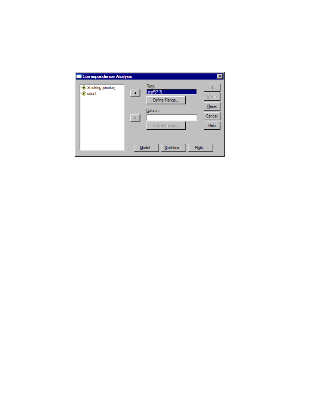
61
Figure 5-1
Correspondence Analysis dialo g box
E Select a row variable.
E Select a column variable.
E Define the ranges for the variables.
E Click OK.
Correspondenc
eAnalysis
Define Row Range in Correspondence Analysis
You must define a range for the row variable. The minimum and maximum values
specified must be integers. Fractional data values are truncated in the analysis. A
categor
y value that is outside of the specified range is ignored in the analysis.
Page 78
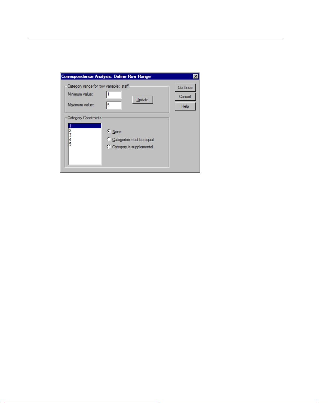
62
Chapter 5
Figure 5-2
Define Row Range dialog box
All categories are initially unconstrained and active. You can constrain row categories
to equal other row categories, or you can define a row category as supplementary.
Categories must be equal. Categories must have equal scores. Use equality
constraints if the obtained order for the categories is undesirable or
counter
intuitive. The maximum number of row categories that can be constrained
to be equal is the total number of active row categories minus 1. To impose
different equality constraints on sets of categories, use syntax. For example, use
syntax
toconstraincategories1and2tobeequalandcategories3and4tobe
equal.
Category is supplemental. Supplementary categories do not influence the analysis
but are represented in the space defined by the active categories. Supplementary
ries play no role in defining the dimensions. The maximum number of
catego
supplementary row categories is the total number of row categories minus 2.
Define Column Range in Correspondence Analysis
You must define a range for the column variable. The minimum and maximum values
specified must be integers. Fractional data values are truncated in the analysis. A
ory value that is outside of the specified range is ignored in the analysis.
categ
Page 79
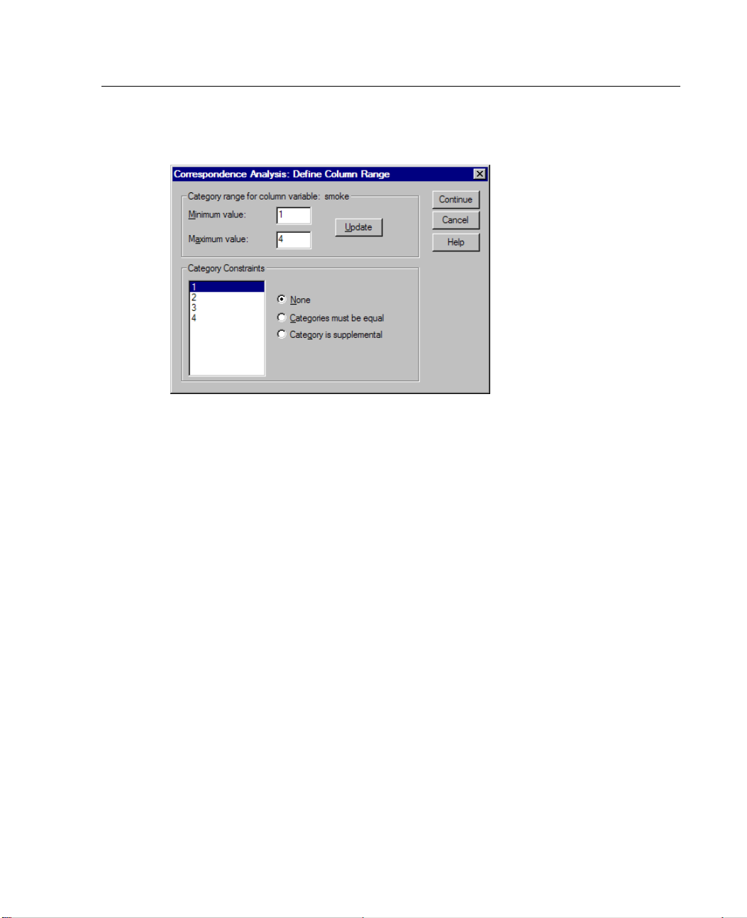
63
Correspondenc
Figure 5-3
Define Column Range dialog box
eAnalysis
All categories are initially unconstrained and active. You can constrain column
categories to equal other column categories, or you can define a column category
as suppl
Catego
ementary.
ries must be equal.
Categories must have equal scores. Use equality
constraints if the obtained order for the categories is undesirable or
counterintuitive. The maximum number of column categories that can be
ained to be equal is the total number of active column categories minus 1.
constr
To impose different equality constraints on sets of categories, use syntax. For
example, use syntax to constrain categories 1 and 2 to be equal and categories
3and4t
Categ
obeequal.
ory is supplemental.
Supplementary categories do not influence the analysis
but are represented in the space defined by the active categories. Supplementary
categories play no role in defining the dimensions. The maximum number of
ementary column categories is the total number of column categories
suppl
minus 2.
Correspondence Analysis Model
The Model dialog box allows you to specify the number of dimensions, the distance
measure, the standardization method, and the normalization method.
Page 80
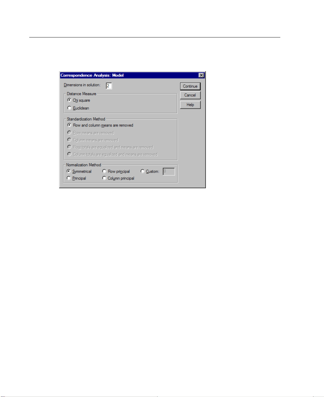
64
Chapter 5
Figure 5-4
Model dialog box
Dimensions in solution. Specify the number of dimensions. In general, choose as few
dimensions as needed to explain most of the variation. The maximum number of
dimensions depends on the number of active categories used in the analysis and on
the equality constraints. The maximum number of dimensions is the smaller of:
The number of active row categories minus the number of row categories
constrained to be equal, plus the number of constrained row category sets.
The number of active column categories minus the number of column categories
constrained to be equal, plus the number of constrained column category sets.
Distance Measure. You can select the measure of distance among the rows and
columns of the correspondence table. Choose one of the following alternatives:
Chi square. Use a weighted profile distance, where the weight is the mass of the
rows or columns. This measure is required for standard correspondence analysis.
Euclidean. Use the square root of the sum of squared differences between pairs of
rows and pairs of columns.
Standardization Method. Choose one of the following alternatives:
Row and column means are removed. Both the rows and columns are centered.
This method is required for standard correspondence analysis.
Page 81

65
Correspondenc
Row m eans are removed. Only the rows are centered.
Column means are removed. Only the columns are centered.
Row totals are equalized and means are removed. Before centering the rows, the
row margins a
Column tota
re equalized.
ls are equalized and means are removed.
Before centering the columns,
eAnalysis
the column margins are equalized.
Normalizat
Symmetrica
ion M ethod.
l.
Choose one of the following alternatives:
For each dimension, the row scores are the weighted average of the
column scores divided by the matching singular value, and the column scores
are the weighted average of row scores divided by the matching singular value.
Use this met
hod if you want to examine the differences or similarities between
the categories of the two variables.
Principal. The distances between row points and column points are
approximations of the distances in the correspondence table according to the
selected d
istance measure. Use this method if you want to examine differences
between categories of either or both variables instead of differences between
the two variables.
Row principal. The distances between row points are approximations of the
distance
s in the correspondence table according to the selected distance measure.
The row scores are the weighted average of the column scores. Use this method
if you want to examine differences or similarities between categories of the
row varia
Column p
ble.
rincipal.
The distances between column points are approximations of
the distances in the correspondence table according to the selected distance
measure. The column scores are the weighted average of the row scores. Use this
method i
f you want to examine differences or similarities between categories of
the column variable.
Custom. You must specify a value between –1 and 1. A value of –1 corresponds
to column principal. A value of 1 corresponds to row principal. A value of 0
ponds to symmetrical. All other values spread the inertia over both the
corres
row and column scores to varying degrees. This method is useful for making
tailor-made biplots.
Page 82

66
Chapter 5
Corresponde
The Statistics dialog box allows you to specify the numerical output produced.
Figure 5-5
Statistics d
Correspondence table. A crosstabulation of the input variables with row and column
marginal
Overview of row points. For each row category, the scores, mass, inertia, contribution
to the inertia of the dimension, and the contribution of the dimension to the inertia
of the poi
Overview of column points. For each column category, the scores, mass, inertia,
contribution to the inertia of the dimension, and the contribution of the dimension to
the iner
nce Analysis Statistics
ialog box
totals.
nt.
tia of the point.
Row profiles. For each row category, the distribution across the categories of the
column variable.
Column p
rofiles.
For each column category, the distribution across the categories of
the row variable.
Permutations of the correspondence table. The correspondence table reorganized such
that the
rows and columns are in increasing order according to the scores on the
first dimension. Optionally, you can specify the maximum dimension number for
which permuted tables will be produced. A permuted table for each dimension from
1tothe
Confidence Statistics for Row points. Includes standard deviation and correlations
number specified is produced.
for all nonsupplementary row points.
Page 83
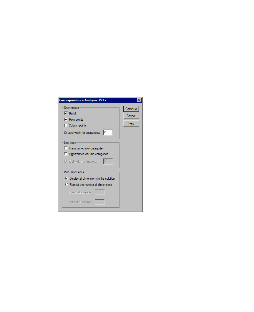
67
Confidence Statistics for Column points. Includes standard deviation and correlations
for all nonsupplementary column points.
Correspondence Analysis Plots
The Plots dialog box allows you to specify which plots are produced.
Figure 5-6
Plots dialog box
Correspondenc
eAnalysis
Scatterplots. Produces a matrix of all pairwise plots of the dimensions. Available
scatterplots include:
Biplot. Produces a matrix of joint plots of the row and column points. If principal
normalization is selected, the biplot is not available.
Row points. Produces a matrix of plots of the row points.
Column points. Produces a matrix of plots of the column points.
Optionally, you can specify how many value label characters to use when labeling the
s. This value must be a non-negative integer less than or equal to 20.
point
Page 84

68
Chapter 5
Line plots. Produces a plot for every dimension of the selected variable. Available
line plots include:
Transformed row categories. Produces a plot of the original row category values
against their corresponding row scores.
Transformed column categories. Produces a plot of the original column category
values agai
nst their corresponding column scores.
Optionally, you can specify how many value label characters to use when labeling the
category axis. This value must be a non-negative integer less than or equal to 20.
ions.
Plot Dimens
Display al
Allows you to control the dimensions displayed in the output.
l dimensions in the solution.
All dimensions in the solution are displayed
in a scatterplot matrix.
Restrict the number of dimensions. The displayed dimensions are restricted to
plotted pairs. If you restrict the dimensions, you must select the lowest and
highest di
mensions to be plotted. The lowest dimension can range from 1 to the
number of dimensions in the solution minus 1, and is plotted against higher
dimensions. The highest dimension value can range from 2 to the number
of dimensi
ons in the solution, and indicates the highest dimension to be used
in plotting the dimension pairs. This specification applies to all requested
multidimensional plots.
CORRESPO
You can customize your correspondence analysis if you paste your selections into a
syntax window and edit the resulting CORRESPONDENCE command syntax. SPSS
command
Specif
Specify the number of value-label characters used to label points for each type of
Specify the number of value-label characters used to label points for each type of
Write a
NDENCE Command Additional Features
language also allows you to:
y table data as input instead of using casewise data (using the
=ALL
scatterplot matrix or biplot matrix (with the
line plo
OUTFILE subcommand).
subcommand).
PLOT subcommand).
t (with the
PLOT subcommand).
matrix of row and column scores to an SPSS matrix data file (with the
TABLE
Page 85

69
Correspondenc
Write a matrix of c onfidence statistics (variances and covariances) for the
singular va
lues and the scores to an SPSS matrix data file (with the
eAnalysis
OUTFILE
subcommand).
Specify multiple sets of categories to be equal (with the EQUAL subcommand).
Page 86

Page 87

Chapter
6
Multiple Cor
Multiple Correspondence Analysis quantifies nominal (categorical) data by assigning
numerical values to the cases (objects) and categories so that objects within the same
category are close together and objects in different categories are far apart. Each
object is as close as possible to the category points of categories that apply to the
object. In this way, the categories divide the objects into homogeneous subgroups.
Variables are considered homogeneous when they classify objects in the same
categories into the same subgroups.
Example. Multiple Correspondence Analysis could be used to graphically display the
relationship between job category, minority classification, and gender. You might
find that minority classification and gender discriminate between people but that
job category does not. You might also find that the Latino and African-American
categories are similar to each other.
Statistics and plots. Object scores, discrimination measures, iteration history,
correlations of original and transformed variables, category quantifications,
descriptive statistics, object points plots, biplots, category plots, joint category plots,
transformation plots, and discrimination measures plots.
respondence Analysis
Data. String variable values are always converted into positive integers by ascending
alphanumeric order. User-defined missing values, system-missing values, and values
less than 1 are considered missing; you can recode or add a constant to variables with
values less than 1 to make them nonmissing.
Assumptions. All variables have the multiple nominal scaling level. The data must
contain at least three valid cases. The analysis is based on positive integer data.
The discretization option will automatically categorize a fractional-valued variable
by grouping its values into categories with a close to “normal” distribution and
will automatically convert values of string variables into positive integers. You can
specify other discretization schemes.
71
Page 88
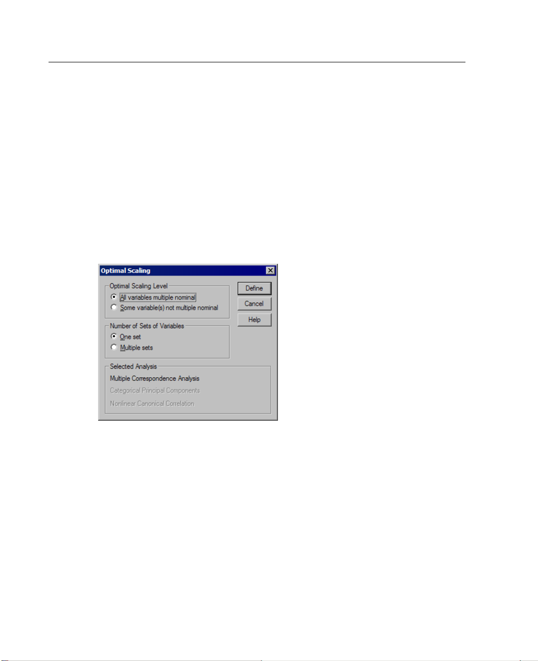
72
Chapter 6
Related procedures. For two variables, Multiple Correspondence Analysis is analogous
to Correspondence Analysis. If you believethat variables possess ordinal or numerical
properties
, Categorical Principal Components Analysis should be used. If sets of
variables are of interest, Nonlinear Canonical Correlation Analysis should be used.
To Obtain a M
E From the me
Analyze
Data Reduction
Optimal Scaling...
Figure 6-1
Optimal Sca
E Select All variables multiple nominal.
E Select One set.
ultiple Correspondence Analysis
nus choose:
ling dialog box
E Click Define.
Page 89
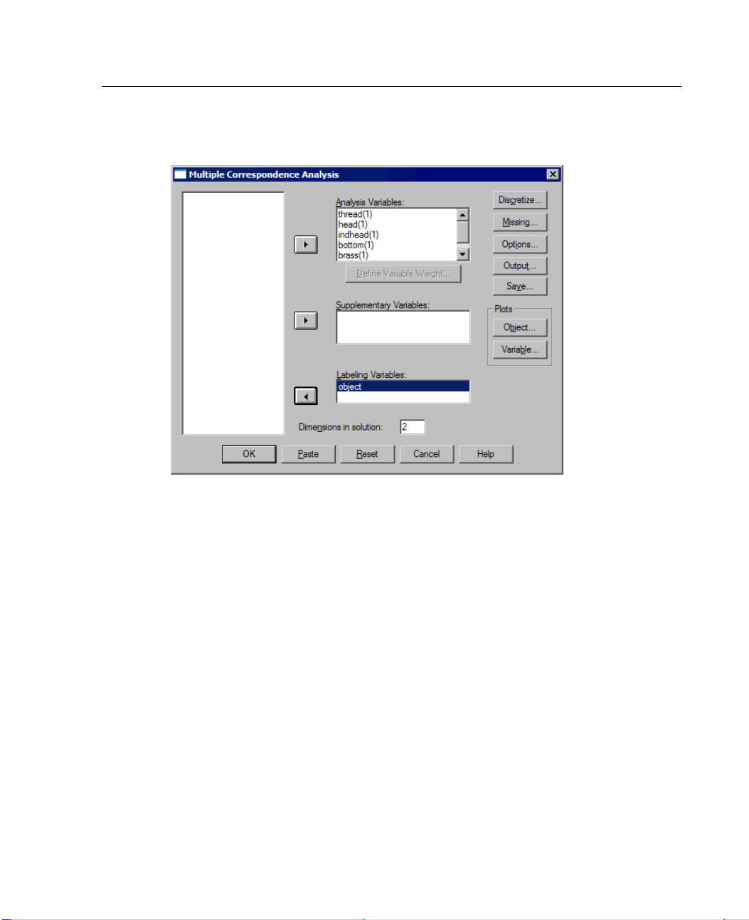
73
Multiple Corre
Figure 6-2
Multiple Correspondence Analysis dialog box
E Select at least two analysis variables and specify the number of dimensions in the
spondence Analysis
solution.
E Click OK.
You may optionally specify supplementary variables, which are fitted into the solution
found, or labeling variables for the plots.
Define Variable Weight in M ultiple Correspondence Analysis
You can set the weight for analysis variables.
Page 90
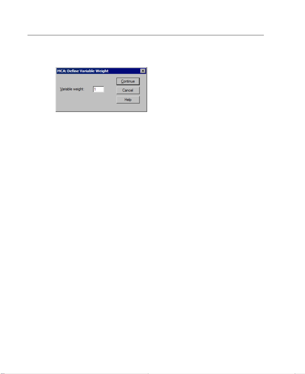
74
Chapter 6
Figure 6-3
Define Variable Weight dialog box
Variable weight. You can choose to define a weight for each variable. The value
specified must be a positive integer. The default value is 1.
Multiple Correspondence Analysis Discretization
The Discretization dialog box allows youtoselectamethodofrecodingyour
variables. Fractional-valued variables are grouped into seven categories (or into the
number of
approximately normal distribution unless otherwise specified. String variables are
always converted into positive integers by assigning category indicators according
to ascen
these integers. Other variables are left alone by default. The discretized variables
arethenusedintheanalysis.
distinct values of the variable if this number is less than seven) with an
ding alphanumeric order. Discretization for string variables applies to
Page 91
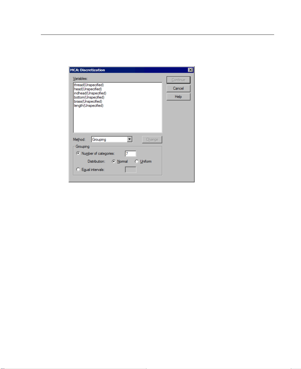
75
Multiple Corre
Figure 6-4
Discretization dialog box
Method. Choose between grouping, ranking, and multiplying.
Grouping. Recode into a specified number of categories or recode by interval.
Ranking. The variable is discretized by ranking the cases.
Multiplying. The current values of the variable are standardized, multiplied by 10,
spondence Analysis
rounded, and have a constant added so that the lowest discretized value is 1.
Grouping. The following options are available when discretizing variables by grouping:
Number of categories. Specify a number of categories and whether the values of
the variable should follow an approximately normal or uniform distribution
those categories.
across
Equal i
ntervals.
Variables are recoded into categories defined by these equally
sized intervals. You must specify the length of the intervals.
Multiple Correspondence Analysis Missing Values
The Missing Values dialog box allows you to choose the strategy for handling missing
values in analysis variables and supplementary variables.
Page 92
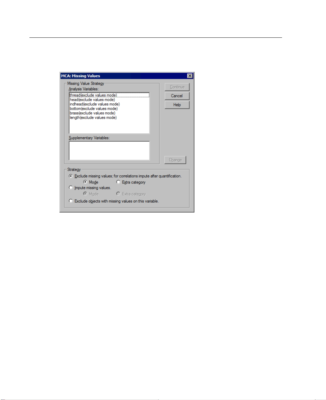
76
Chapter 6
Figure 6-5
Missing Values dialog box
Missing Value Strategy. Choose to exclude missing values (passive treatment), impute
missing values (active treatment), or exclude objects with missing values (listwise
on).
deleti
Exclu
de missing values; for correlations impute after quantification.
Objects with
missing values on the selected variable do not contribute to the analysis for this
variable. If all variables are given passive treatment, then objects with missing
s on all variables are treated as supplementary. If correlations are specified
value
in the Output dialog box, then (after analysis) missing values are imputed with the
most frequent category, or mode, of the variable for the correlations of the original
bles. For the correlations of the optimally scaled variables, you can choose
varia
the method of imputation. Select
the optimally scaled variable. Select
uantification of an extra category. This implies that objects with a missing
the q
Mode to replace missing values with the mode of
Extra category to replace missing values with
value on this variable are considered to belong to the same (extra) category.
Page 93

77
Impute missing values. Objects with missing values on the selected variable have
those value
s imputed. You can choose the method of imputation. Select
replace missing values with the most frequent category. When there are multiple
modes, the one with the smallest category indicator is used. Select
to replace m
issing values with the same quantification of an extra category.
This implies that objects with a missing value on this variable are considered to
belong to the same (extra) category.
Exclude objects with missing values on this variable. Objects with missing values
on the sele
cted variable are excluded from the analysis. This strategy is not
available for supplementary variables.
Multiple Correspondence Analysis Options
The Options dialog box allows you to select the initial configuration, specify iteration
and convergence criteria, select a normalization method, choose the method for
labeling
plots, and specify supplementary objects.
Multiple Corre
spondence Analysis
Mode to
Extra category
Page 94
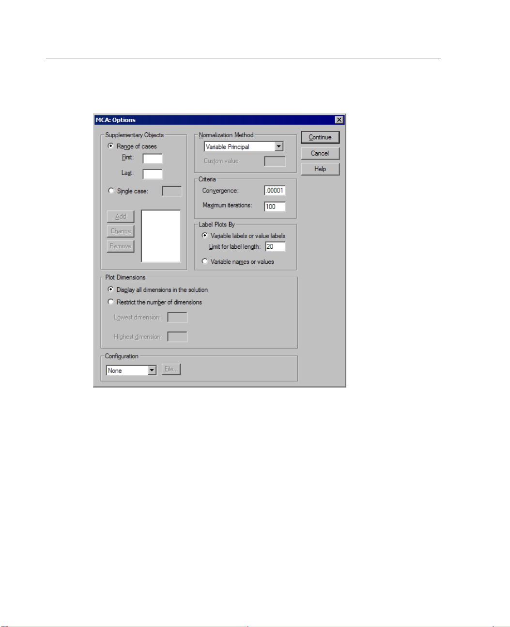
78
Chapter 6
Figure 6-6
Options dialog box
Supplementary Objects. Specify the case number of the object, or the first and last case
numbers of a range of objects, that you want to make supplementary, and then click
Add. Continue until you have specified all of your supplementary objects. If an object
is specified as supplementary, then case weights are ignored for that object.
Normalization Method. You can specify one of five options for normalizing the
object scores and the variables. Only one normalization method can be used in
a given analysis.
Variable Principal. This option optimizes the association between variables. The
coordinates of the variables in the object space are the component loadings
(correlations with principal components, such as dimensions and object scores).
This is useful when you are interested primarily in the correlation between the
variables.
Page 95

79
Multiple Corre
Object Principal. This option optimizes distances between objects. This is useful
when you are
interested primarily in differences or similarities between the
spondence Analysis
objects.
Symmetrical. Use this normalization option if you are interested primarily in the
relation between objects and variables.
Independent. Use this normalization option if you want to examine distances
between obj
Custom. Yo
ects and correlations between variables separately.
u can specify any real value in the closed interval [–1, 1]. A value of 1
is equal to the Object Principal method, a value of 0 is equal to the Symmetrical
method, and a value of –1 is equal to the Variable Principal method. By
specifyin
g a value greater than –1 and less than 1, you can spread the eigenvalue
over both objects and variables. This method is useful for making a tailor-made
biplot or triplot.
Criteria. You can specify the maximum number of iterations the procedure can go
through i
n its computations. You can also select a convergence criterion value. The
algorithm stops iterating if the difference in total fit between the last two iterations is
less than the convergence value or if the maximum number of iterations is reached.
ts By.
Label Plo
Allows you to specify whether variables and value labels or variable
names and values will be used in the plots. You can also specify a maximum length
for labels.
Plot Dime
Display
nsions.
Allows you to control the dimensions displayed in the output.
all dimensions in the solution.
All dimensions in the solution are displayed
in a scatterplot matrix.
Restrict the number of dimensions. The displayed dimensions are restricted to
plotted pairs. If you restrict the dimensions, you must select the lowest and
highest
dimensions to be plotted. The lowest dimension can range from 1 to the
number of dimensions in the solution minus 1 and is plotted against higher
dimensions. The highest dimension value can range from 2 to the number of
dimens
ions in the solution and indicates the highest dimension to be used
in plotting the dimension pairs. This specification applies to all requested
multidimensional plots.
Page 96

80
Chapter 6
Configuration. You can read data from a file containing the coordinates of a
configuration. The first variable in the file should contain the coordinates for the
first dimen
sion, the second variable should contain the coordinates for the second
dimension, and so on.
Initial. The configuration in the file specified will be used as the starting point
of the analy
Fixed. The
sis.
configuration in the file specified will be used to fit in the variables.
The variables that are fitted in must be selected as analysis variables, but, because
the configuration is fixed, they are treated as supplementary variables (so they do
not need to
be selected as supplementary variables).
Multiple Correspondence Analysis Output
The Output dialog box allows you to produce tables for object scores, discrimination
measures
category quantifications for selected variables, and descriptive statistics for selected
variables.
, iteration history, correlations of original and transformed variables,
Page 97
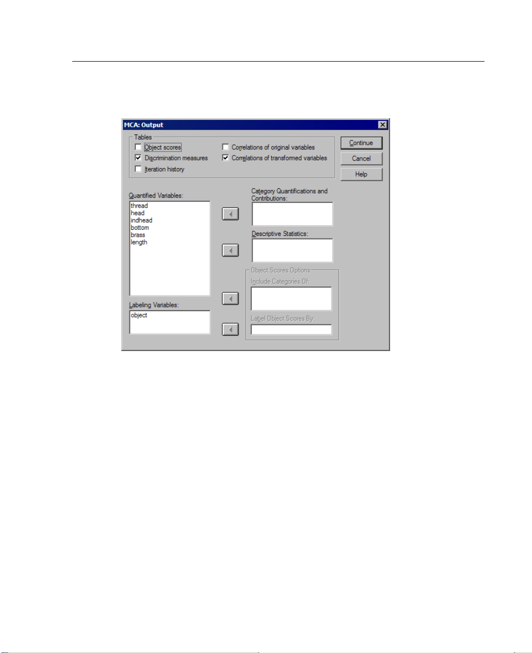
81
Figure 6-7
Output dialog box
Multiple Corre
spondence Analysis
Object scores. Displays the object scores, including mass, inertia, and contributions,
and has
Inclu
the following options:
de Cate gories Of.
Displays the category indicators of the analysis variables
selected.
Label Object Scores By. From the list of variables specified as labeling variables,
you can select one to label the objects.
Discrimination measures. Displays the discrimination measures per variable and
per dim
Iteration history. For each iteration, the variance accounted for, loss, and increase
ension.
in variance accounted for are shown.
lations of original variables.
Corre
Shows the correlation matrix of the original variables
and the eigenvalues of that matrix.
Correlations of transformed variables. Shows the correlation matrix of the transformed
mally scaled) variables and the eigenvalues of that matrix.
(opti
Page 98
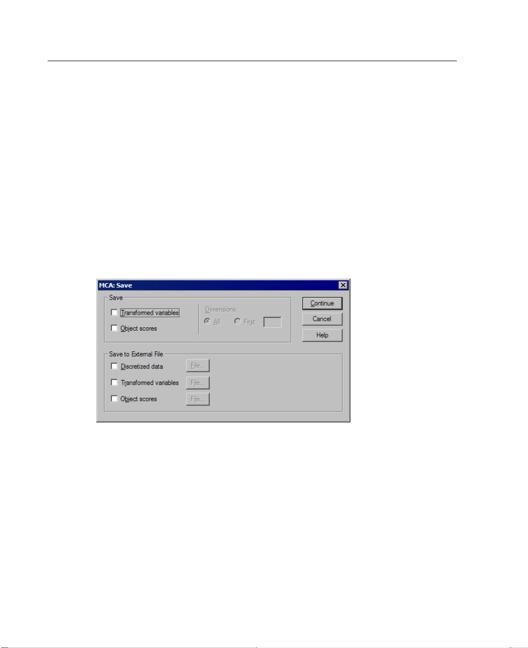
82
Chapter 6
Category Quantifications and Contributions. Gives the category quantifications
(coordinates), including mass, inertia, and contributions, for each dimension of
the variabl
Descriptive Statistics. Displays frequencies, number of missing values, and mode of
the variable(s) selected.
e(s) selected.
Multiple Correspondence Analysis Save
The Save dialog box allows you to add the transformed variables and object scores to
the working data file or as new variables in external files and to save the discretized
data as new
Figure 6-8
Save dialog box
variables in an external data file.
Save. S
saved must be specified.
Save to External File. Save selections to a new external file. Specify a filename for
each se
ave selections to the working data file. The number of dimensions to be
lected option by clicking
File. Each file specified must have a different name.
Multiple Correspondence Analysis Object Plots
The Object Plots dialog box allows you to specify the types of plots desired and the
bles for which plots will be produced.
varia
Page 99
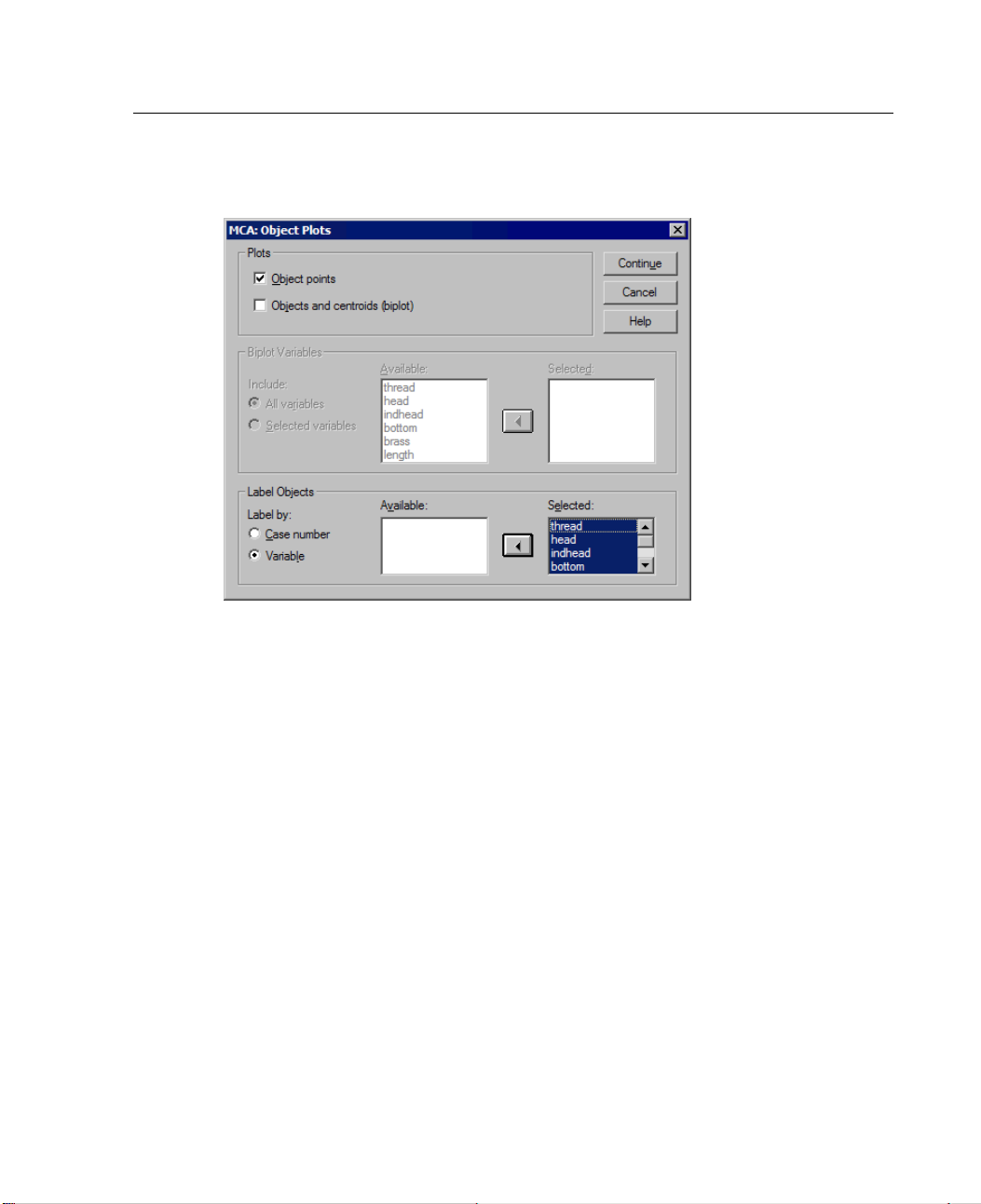
83
Figure 6-9
Object Plots dialog box
Object points. A plot of the object points is displayed.
Multiple Corre
spondence Analysis
Objects and centroids (biplot). The object points are plotted with the variable centroids.
Biplot Variables. You can choose to use all variables for the biplots or select a subset.
Label Objects. You can choose to have objects labeled with the categories of selected
variables ( you may choose category indicator values or value labels in the Options
dialog box) or with their case numbers. One plot is produced per variable if
selected.
Multiple Correspondence Analysis Variable Plots
The Variable Plots dialog box allows you to specify the types of plots desired and the
variables for which plots will be produced.
Variable is
Page 100
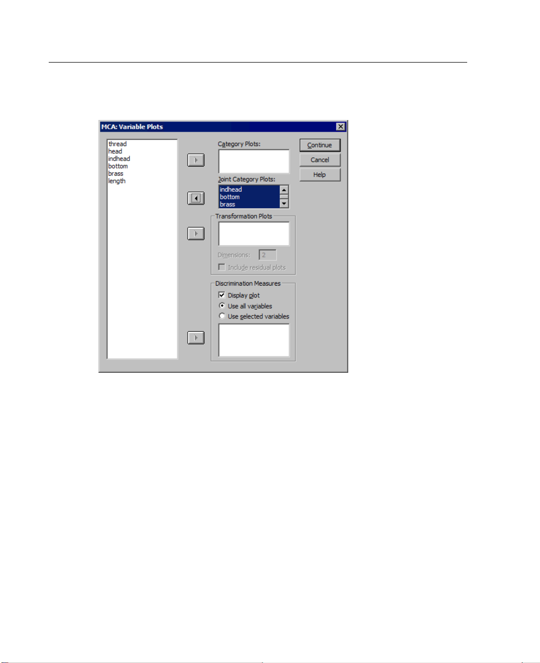
84
Chapter 6
Figure 6-10
Variable Plots dialog box
Category Plots. For each variable selected, a plot of the centroid coordinates is plotted.
Categories are in the centroids of the objects in the particular categories.
Joint Category Plots. This is a single plot of the centroid coordinates of each selected
variable.
Transformation Plots. Displays a plot of the optimal category quantifications versus
the category indicators. You can specify the number of dimensions desired; one
plot will be generated for each dimension. You can also choose to display residual
plots for each variable selected.
Discrimination M easures. Produces a single plot of the discrimination measures for
the selected variables.
 Loading...