

Page 1

SPSS Categories® 11.0
Jacqueline J. Meulman
Willem J. Heiser
SPSS Inc.
Page 2

For more information about SPSS® software products, please visit our Web site at
http://www.spss.com or contact
SPSS Inc.
233 South Wacker Drive, 11th Floor
Chicago, IL 60606-6412
Tel: (312) 651-3000
Fax: (312) 651-3668
SPSS is a registered trademark and the other product names are the trademarks of SPSS
Inc. for its proprietary computer software. No material describing such software may be
produced or distributed without the written permission of the owners of the trademark
and license rights in the software and the copyrights in the published materials.
The SOFTWARE and documentation are provided with RESTRICTED RIGHTS.
Use, duplication, or disclosure by the Government is subject to restrictions as set
forth in subdivision (c)(1)(ii) of The Rights in Technical Data and Computer
Software clause at 52.227-7013. Contractor/manufacturer is SPSS Inc., 233 South
Wacker Drive, 11th Floor, Chicago, IL 60606-6412.
General notice: Other product names mentioned herein are used for identification
purposes only and may be trademarks of their respective companies.
TableLook is a trademark of SPSS Inc.
Windows is a registered trademark of Microsoft Corporation.
Portions of this product were created using LEADTOOLS © 1991–2000, LEAD
Technologies, Inc. ALL RIGHTS RESERVED.
LEAD, LEADTOOLS, and LEADVIEW are registered trademarks of LEAD
Technologies, Inc.
Portions of this product were based on the work of the FreeType Team
(http://www.freetype.org).
®
SPSS Categories
11.0
Copyright © 2001 by SPSS Inc.
All rights reserved.
Printed in the United States of America.
No part of this publication may be reproduced, stored in a retrieval system, or transmitted, in any form or by any means, electronic, mechanical, photocopying, recording,
or otherwise, without the prior written permission of the publisher.
1 2 3 4 5 6 7 8 9 0 05 04 03 02 01
ISBN 1-56827-276-6
Page 3

Preface
SPSS 11.0 is a powerful software package for microcomputer data management and
analysis. The Categories option is an add-on enhancement that provides a comprehensive set of procedures for optimal scaling. The procedures in Categories must be
used with the SPSS 11.0 Base and are completely integrated into that system.
The Categories option includes procedures for:
• Categorical regression
• Categorical principal components analysis
• Nonlinear canonical correlation analysis
• Correspondence analysis
• Homogeneity analysis
• Multidimensional scaling
Installation
Compatibility
Serial Numbers
To install Categories, follow the instructions for adding and removing features in the
installation instructions supplied with the SPSS Base. (To start, double-click on the
SPSS Setup icon.)
The SPSS system is designed to operate on many computer systems. See the materials
that came with your system for specific information on minimum and recommended
requirements.
Your serial number is your identification number with SPSS Inc. You will need this
serial number when you call SPSS Inc. for information regarding support, payment, or
an upgraded system. The serial number was provided with your Base system. Before
using the system, please copy this number to the registration card.
iii
Page 4

Registration Card
Don’t put it off: fill out and send us your registration card. Until we receive your
registration card, you have an unregistered system. Even if you have previously sent a
card to us, please fill out and return the card enclosed in your Categories package.
Registering your system entitles you to:
• Technical support services
• New product announcements and upgrade announcements
Customer Service
If you have any questions concerning your shipment or account, contact your local
office, listed on page vi. Please have your serial number ready for identification when
calling.
Training Seminars
SPSS Inc. provides both public and onsite training seminars for SPSS. All seminars
feature hands-on workshops. SPSS seminars will be offered in major U.S. and
European cities on a regular basis. For more information on these seminars, call your
local office, listed on page vi.
Technical Support
The services of SPSS Technical Support are available to registered customers.
Customers may call Technical Support for assistance in using SPSS products or for
installation help for one of the supported hardware environments. To reach Technical
Support, see the SPSS Web site at http://www.spss.com, or call your local office, listed
on page vi. Be prepared to identify yourself, your organization, and the serial number
of your system.
Additional Publications
Except for academic course adoptions, additional copies of SPSS product manuals can
be purchased directly from SPSS Inc. Visit our Web site at http://www.spss.com, or
contact your local SPSS office, listed on page vi.
SPSS product manuals may also be purchased from Prentice Hall, the exclusive distributor of SPSS publications. To order, fill out and mail the Publications order form
included with your system, or call 800-947-7700. If you represent a bookstore or have
an account with Prentice Hall, call 800-382-3419. In Canada, call 800-567-3800. Outside of North America, contact your local Prentice Hall office.
iv
Page 5

Tell Us Your Thoughts
Your comments are important. Please let us know about your experiences with SPSS
products. We especially like to hear about new and interesting applications using the
SPSS system. Please send e-mail to [email protected], or write to SPSS Inc., Attn:
Director of Product Planning, 233 South Wacker Drive, 11th Floor, Chicago, IL
60606-6412.
About This Manual
This manual is divided into two sections. The first section documents the graphical
user interface and provides examples of the statistical techniques available. In addition, this section offers advice on interpreting the output. The second part of the manual
is a Syntax Reference section that provides complete command syntax for all of the
commands included in the Categories option. Most features of the system can be accessed through the dialog box interface, but some functionality can be accessed only
through command syntax.
This manual contains two indexes: a subject index and a syntax index. The subject
index covers both sections of the manual. The syntax index applies only to the Syntax
Reference section.
Acknowledgments
Contacting SPSS
The optimal scaling procedures and their SPSS implementation were developed by the
Data Theory Scaling System Group (DTSS), consisting of members of the departments
of Education and Psychology of the Faculty of Social and Behavioral Sciences at
Leiden University.
Willem Heiser, Jacqueline Meulman, Gerda van den Berg, and Patrick Groenen
were involved with the original 1990 procedures. Jacqueline Meulman and Peter
Neufeglise participated in the development of procedures for categorical regression,
correspondence analysis, categorical principal components analysis, and multidimensional scaling. In addition, Anita van der Kooij contributed especially to
CATREG, CORRESPONDENCE, and CATPCA, and Frank Busing and Willem
Heiser, to the PROXSCAL procedure. The development of PROXSCAL has profited
from technical comments and suggestions from Jacques Commandeur and Patrick
Groenen.
If you would like to be on our mailing list, contact one of our offices, listed on page vi,
or visit our Web site at http://www.spss.com. We will send you a copy of our newsletter
and let you know about SPSS Inc. activities in your area.
v
Page 6

SPSS Inc.
Chicago, Illinois, U.S.A.
Tel: 1.312.651.3000
or 1.800.543.2185
www.spss.com/corpinfo
Customer Service:
1.800.521.1337
Sales:
1.800.543.2185
[email protected]
Training:
1.800.543.6607
Technical Support:
1.312.651.3410
[email protected]
SPSS Federal Systems
Tel: 1.703.740.2400
or 1.800.860.5762
www.spss.com
SPSS Argentina srl
Tel: +5411.4814.5030
www.spss.com
SPSS Asia Pacific Pte. Ltd.
Tel: +65.245.9110
www.spss.com
SPSS Australasia Pty. Ltd.
Tel: +61.2.9954.5660
www.spss.com
SPSS Belgium
Tel: +32.163.170.70
www.spss.com
SPSS Benelux BV
Tel: +31.183.651777
www.spss.com
SPSS Brasil Ltda
Tel: +55.11.5505.3644
www.spss.com
SPSS Czech Republic
Tel: +420.2.24813839
www.spss.cz
SPSS Denmark
Tel: +45.45.46.02.00
www.spss.com
SPSS East Africa
Tel: +254 2 577 262
spss.com
SPSS Finland Oy
Tel: +358.9.4355.920
www.spss.com
SPSS France SARL
Tel: +01.55.35.27.00
www.spss.com
SPSS Germany
Tel: +49.89.4890740
www.spss.com
SPSS BI Greece
Tel: +30.1.6971950
www.spss.com
SPSS Iberica
Tel: +34.902.123.606
SPSS.com
SPSS Hong Kong Ltd.
Tel: +852.2.811.9662
www.spss.com
SPSS Ireland
Tel: +353.1.415.0234
www.spss.com
SPSS BI Israel
Tel: +972.3.6166616
www.spss.com
SPSS Italia srl
Tel: +800.437300
www.spss.it
SPSS Japan Inc.
Tel: +81.3.5466.5511
www.spss.co.jp
SPSS Korea DataSolution Co.
Tel: +82.2.563.0014
www.spss.co.kr
SPSS Latin America
Tel: +1.312.651.3539
www.spss.com
SPSS Malaysia Sdn Bhd
Tel: +603.6203.2300
www.spss.com
SPSS Miami
Tel: 1.305.627.5700
SPSS.com
SPSS Mexico SA de CV
Tel: +52.5.682.87.68
www.spss.com
SPSS Norway AS
Tel: +47.22.99.25.50
www.spss.com
SPSS Polska
Tel: +48.12.6369680
www.spss.pl
SPSS Russia
Tel: +7.095.125.0069
www.spss.com
SPSS San Bruno
Tel: 1.650.794.2692
www.spss.com
SPSS Schweiz AG
Tel: +41.1.266.90.30
www.spss.com
SPSS BI (Singapore) Pte. Ltd.
Tel: +65.346.2061
www.spss.com
SPSS South Africa
Tel: +27.21.7120929
www.spss.com
SPSS South Asia
Tel: +91.80.2088069
www.spss.com
SPSS Sweden AB
Tel: +46.8.506.105.50
www.spss.com
SPSS Taiwan Corp.
Taipei, Republic of China
Tel: +886.2.25771100
www.sinter.com.tw/spss/main
SPSS (Thailand) Co., Ltd.
Tel: +66.2.260.7070
www.spss.com
SPSS UK Ltd.
Tel: +44.1483.719200
www.spss.com
vi
Page 7

Contents
1 Introduction to SPSS Optimal Scaling Procedures for
Categorical Data 1
What Is Optimal Scaling? 1
Why Use Optimal Scaling? 1
Optimal Scaling Level and Measurement Level 2
Selecting the Optimal Scaling Level 3
Transformation Plots 4
Category Codes 5
Which Procedure Is Best for Your Application? 7
Categorical Regression 8
Categorical Principal Components Analysis 9
Nonlinear Canonical Correlation Analysis 9
Correspondence Analysis 10
Homogeneity Analysis 12
Multidimensional Scaling 13
Displays with More than Two Dimensions 14
Three-Dimensional Scatterplots 14
Scatterplot Matrices 15
Aspect Ratio in Optimal Scaling Charts 16
2 Categorical Regression (CATREG) 17
To Obtain a Categorical Regression 18
Define Scale in Categorical Regression 19
To Define the Scale in CATREG 20
Categorical Regression Discretization 20
Categorical Regression Missing Values 22
Categorical Regression Options 23
Categorical Regression Output 24
Categorical Regression Save 25
Categorical Regression Plots 26
CATREG Command Additional Features 26
vii
Page 8

3 Categorical Principal Components Analysis (CATPCA) 27
To Obtain a Categorical Principal Components Analysis 28
Define Scale and Weight in CATPCA 29
To Define the Scale and Weight in CATPCA 31
Categorical Principal Components Discretization 32
Categorical Principal Components Missing Values 33
Categorical Principal Components Category Plots 34
Categorical Principal Components Object and Variable Plots 35
Categorical Principal Components Loading Plots 36
Categorical Principal Components Output 37
Categorical Principal Components Save 38
Categorical Principal Components Options 39
CATPCA Command Additional Features 40
4 Nonlinear Canonical Correlation Analysis (OVERALS) 41
To Obtain a Nonlinear Canonical Correlation Analysis 42
Define Range and Scale in OVERALS 44
To Define an Optimal Scaling Range and Scale in OVERALS 45
Define Range in OVERALS 45
To Define an Optimal Scaling Range in OVERALS 46
Nonlinear Canonical Correlation Analysis Options 46
OVERALS Command Additional Features 48
5 Correspondence Analysis 49
To Obtain a Correspondence Analysis 50
Define Row Range in Correspondence Analysis 51
To Define a Row Range in Correspondence Analysis 51
Define Column Range in Correspondence Analysis 52
To Define a Column Range in Correspondence Analysis 53
Correspondence Analysis Model 54
Correspondence Analysis Statistics 56
Correspondence Analysis Plots 57
CORRESPONDENCE Command Additional Features 58
viii
Page 9

6 Homogeneity Analysis (HOMALS) 59
To Obtain a Homogeneity Analysis 60
Define Range in Homogeneity Analysis 62
To Define an Optimal Scaling Range in Homogeneity Analysis 62
Homogeneity Analysis Options 63
HOMALS Command Additional Features 64
7 Multidimensional Scaling (PROXSCAL) 65
To Obtain a Multidimensional Scaling 66
Proximities in Matrices across Columns 67
Proximities in Columns 68
Proximities in One Column 69
Create Proximities from Data 70
Measures Dialog Box 71
Define a Multidimensional Scaling Model 72
Multidimensional Scaling Restrictions 74
Multidimensional Scaling Options 75
Multidimensional Scaling Plots, Version 1 76
Multidimensional Scaling Plots, Version 2 78
Multidimensional Scaling Output 78
PROXSCAL Command Additional Features 80
8 Categorical Regression Examples 81
Example 1: Carpet Cleaner Data 81
A Standard Linear Regression Analysis 82
A Categorical Regression Analysis 84
Example 2: Ozone Data 93
Categorizing Variables 94
Selection of Transformation Type 95
Optimality of the Quantifications 101
Effects of Transformations 102
ix
Page 10

9 Categorical Principal Components Analysis Examples 107
Example 1: Interrelations of Social Systems 108
Number of Dimensions 110
Quantifications 111
Object Scores 112
Component Loadings 114
Additional Dimensions 115
Example 2: Symptomatology of Eating Disorders 118
Transformation Plots 121
Model Summary 122
Component Loadings 123
Object Scores 124
Examining the Structure of the Course of Illness 126
10 Nonlinear Canonical Correlation Analysis Examples 131
Example: An Analysis of Survey Results 131
Examining the Data 132
Accounting for Similarity between Sets 134
Component Loadings 138
Transformation Plots 138
Single versus Multiple Category Coordinates 140
Centroids and Projected Centroids 142
An Alternative Analysis 145
General Suggestions 149
11 Correspondence Analysis Examples 151
Example 1: Smoking Behavior by Job Category 152
Profiles and Distances 156
Inertia 157
Row and Column Scores 158
Dimensionality 159
Supplementary Profiles 160
Contributions 162
Permutations of the Correspondence Table 165
Confidence Statistics 166
Normalization 168
x
Page 11

Example 2: Perceptions of Coffee Brands 171
Principal Normalization 172
Dimensionality 172
Contributions 173
Plots 175
Symmetrical Normalization 177
Example 3: Flying Mileage between Cities 178
Row and Column Scores 181
12 Homogeneity Analysi s Examples 183
Example: Characteristics of Hardware 184
Multiple Dimensions 185
Object Scores 186
Discrimination Measures 188
Category Quantifications 189
A More Detailed Look at Object Scores 191
Omission of Outliers 194
13 Multidimensional Scaling Examples 197
Example: An Examination of Kinship Terms 197
Choosing the Number of Dimensions 198
A Three-Dimensional Solution 199
A Three-Dimensional Solution with Nondefault Transformations 205
Discussion 208
Syntax Reference 209
Introduction 211
ANACOR 215
CATPCA 225
CATREG 243
CORRESPONDENCE 255
HOMALS 267
OVERALS 275
xi
Page 12

PRINCALS 285
PROXSCAL 295
Bibliography 313
Subject Index 317
Syntax Index 323
xii
Page 13

1
Introduction to SPSS Optimal Scaling Procedures for Categorical Data
SPSS Categories procedures use optimal scaling to analyze data that are difficult or impossible for “standard” statistical procedures to analyze.
each procedure does, the situations in which each procedure is most appropriate, the relationships between the procedures, and the relationships of these procedures to their
“standard” statistical counterparts.
What Is Optimal Scaling?
The idea behind optimal scaling is to assign numerical quantifications to the categories
of each variable, thus allowing “standard” procedures to be used to obtain a solution on
the quantified variables.
The optimal scale values are assigned to categories of each variable based on the
optimizing criterion of the procedure in use. Unlike the original labels of the nominal
or ordinal variables in the analysis, these scale values have metric properties.
In most Categories procedures, the optimal quantification for each scaled variable is
obtained through an iterative method called alternating least squares in which, after
the current quantifications are used to find a solution, the quantifications are updated
using that solution. The updated quantifications are then used to find a new solution,
which is used to update the quantifications, and so on until some criterion is reached
that signals the process to stop.
Why Use Optimal Scaling?
1
This chapter describes what
Categorical data are often found in marketing research, survey research, and research
in the social and behavioral sciences. In fact, many researchers deal almost exclusively
with categorical data.
1. These procedures and their SPSS implementation were developed by the Data Theory Scaling System Group (DTSS), consisting of members of the departments of Education and Psychology, Faculty of Social and Behavioral Sciences, Leiden
University.
1
Page 14
2 Chapter 1
While adaptations of most standard models exist specifically to analyze categorical
data, they often do not perform well for data sets that feature:
• Too few observations
• Too many variables
• Too many values per variable
By quantifying categories, optimal scaling techniques avoid problems in these situations. Moreover, they are useful even when specialized techniques are appropriate.
Rather than interpreting parameter estimates, the interpretation of optimal scaling
output is often based on graphical displays. Optimal scaling techniques offer excellent
exploratory analyses, which complement other SPSS models well. By narrowing the
focus of your investigation, visualizing your data through optimal scaling can form the
basis of an analysis that centers on interpretation of model parameters.
Optimal Scaling Level and Measurement Level
This can be a very confusing concept when you first use Categories procedures. When
specifying the level, you specify not the level at which variables are measured, but the
level at which they are scaled. The idea is that the variables to be quantified may have
nonlinear relations regardless of how they are measured.
For Categories purposes, there are three basic levels of measurement:
•The nominal level implies that a variable’s values represent unordered categories.
Examples of variables that might be nominal are region, zip code area, religious af-
filiation, and multiple choice categories.
•The ordinal level implies that a variable’s values represent ordered categories. Ex-
amples include attitude scales representing degree of satisfaction or confidence and
preference rating scores.
•The numerical level implies that a variable’s values represent ordered categories
with a meaningful metric, so that distance comparisons between categories are appropriate. Examples include age in years and income in thousands of dollars.
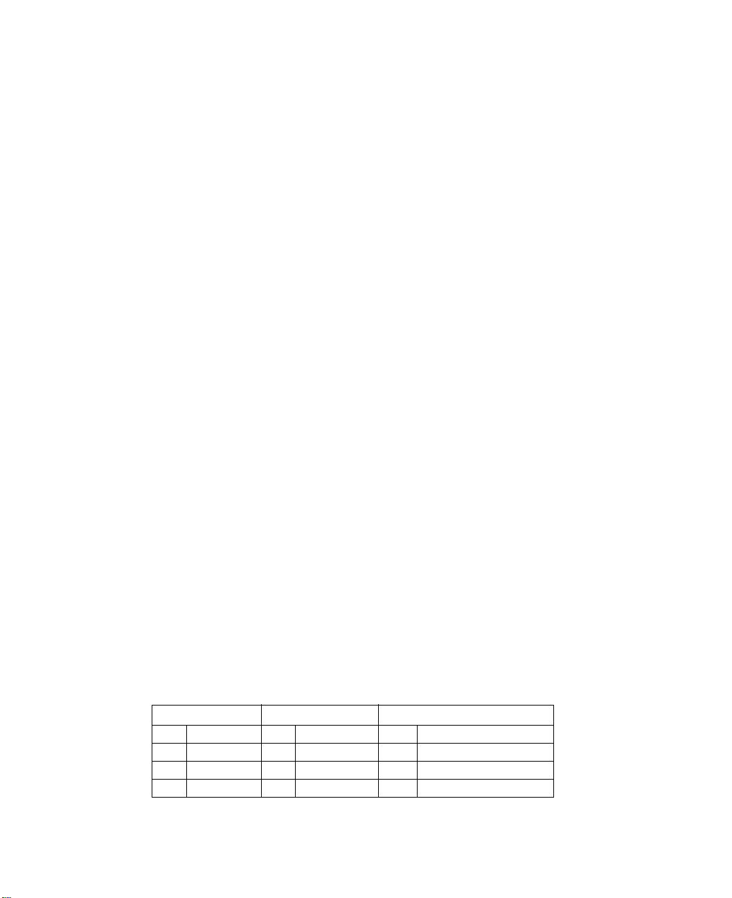
For example, suppose the variables
Table 1.1 Coding scheme for region, job, and age
Region Job Age
1 North 1 intern 20 twenty years old
2 South 2 sales rep 22 twenty-two years old
3 East 3 manager 25 twenty-five years old
4 West 27 twenty-seven years old
region, job, and age are coded as shown in Table 1.1.
Page 15

Introduction to SPSS Optimal Scaling Procedures for Categorical Data 3
The values shown represent the categories of each variable. Region would be a nominal
variable. There are four categories of
through 4 simply represent the four categories; the coding scheme is completely arbitrary.
Job, on the other hand, could be assumed to be an ordinal variable. The original
categories form a progession from intern to manager. Larger codes represent a job higher
on the corporate ladder. However, only the order information is known—nothing can be
said about the distance between adjacent categories. In contrast,
to be a numerical variable. In the case of
trinsically meaningful. The distance between 20 and 22 is the same as the distance between 25 and 27, while the distance between 22 and 25 is greater than either of these.
Selecting the Optimal Scaling Level
It is important to understand that there are no intrinsic properties of a variable that automatically predefine what optimal scaling level you should specify for it. You can explore
your data in any way that makes sense and makes interpretation easier. By analyzing a
numerical-level variable at the ordinal level, for example, the use of a nonlinear transformation may allow a solution in fewer dimensions.
The following two examples illustrate how the “obvious” level of measurement
might not be the best optimal scaling level. Suppose that a variable sorts objects into age
groups. Although age can be scaled as a numerical variable, it may be true that for people younger than 25 safety has a positive relation with age, whereas for people older than
60 safety has a negative relation with age. In this case, it might be better to treat age as
a nominal variable.
As another example, a variable that sorts persons by political preference appears to
be essentially nominal. However, if you order the parties from political left to political
right, you might want the quantification of parties to respect this order by using an ordinal level of analysis.
Even though there are no predefined properties of a variable that make it exclusively
one level or another, there are some general guidelines to help the novice user. With single-nominal quantification, you don’t usually know the order of the categories but you
want the analysis to impose one. If the order of the categories is known, you should try
ordinal quantification. If the categories are unorderable, you might try multiple-nominal
quantification.
region, with no intrinsic ordering. Values 1
age could be assumed
age, the distances between the values are in-
Page 16
4 Chapter 1
Transformation Plots
The different levels at which each variable can be scaled impose different restrictions on
the quantifications. Transformation plots illustrate the relationship between the quantifications and the original categories resulting from the selected optimal scaling level.
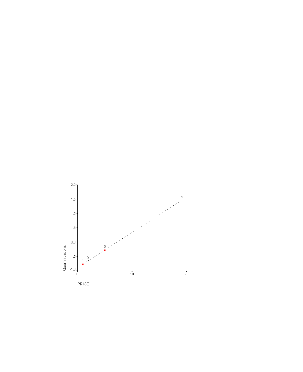
For example, a linear transformation plot results when a variable is treated as numerical.
Variables treated as ordinal result in a nondecreasing transformation plot. Transformation plots for variables treated nominally that are U-shaped (or the reverse) display a
quadratic relationship. Nominal variables could also yield transformation plots without
apparent trends by changing the order of the categories completely. Figure 1.1 displays
a sample transformation plot.
Transformation plots are particularly suited to determining how well the selected
optimal scaling level performs. If several categories receive similar quantifications, collapsing these categories into one category may be warranted. Alternatively, if a variable
treated as nominal receives quantifications that display an increasing trend, an ordinal
transformation may result in a similar fit. If that trend is linear, numerical treatment may
be appropriate. However, if collapsing categories or changing scaling levels is warranted, the analysis will not change significantly.
Figure 1.1 Transformation plot of price (numerical)
Although HOMALS does not currently offer the transformation plot in Figure 1.1 as an
option, creating this plot is a straightforward procedure. For each variable, create a new
variable containing the values (and labels) of the categories. Create a new variable containing the quantifications for that variable from the Categories analysis. Use the line facility with the data in the chart representing the values of individual cases. You can use
the quantifications for the line in the chart and use the categories to label the chart.
Page 17

Category Codes
Some care should be taken when coding categorical variables, because some coding
schemes may yield unwanted output or incomplete analyses. Possible coding schemes
for
Table 1.2 Alternative coding schemes for job
Category A B C D
intern 1 1 5 1
sales rep 2 2 6 5
manager 3 7 7 3
Some Categories procedures require that the range of every variable used be defined.
Any value outside this range is treated as a missing value. The minimum category value
is always 1. The maximum category value is supplied by the user. This value is not the
number of categories for a variable; it is the largest category value. For example, in
Table 1.2, scheme A has a maximum category of 3 and scheme B has a maximum category value of 7, yet both schemes code the same three categories.
Any categories with codes outside the defined range are omitted from the analysis. This
is a simple method for omitting categories but can result in unwanted analyses. An
incorrectly defined maximum category can omit valid categories from the analysis. For
example, for scheme B, defining the maximum category value to be 3 indicates that
has categories coded from 1 to 3; the manager category is treated as missing. Because
no category has actually been coded
cases. If you wanted to omit all manager categories, this analysis would be appropriate.
However, if managers are to be included, the maximum category must be defined as 7,
and missing values must be coded with values above 7 or below 1.
the results. For nominal variables, only the label and not the value associated with that
label is important. For ordinal variables, the order of the categories is preserved in the
quantifications; the category values themselves are not important. All coding schemes
resulting in the same category ordering will have identical results. For example, the first
three schemes in Table 1.2 are functionally equivalent if
level. The order of the categories is identical in these schemes. Scheme D, on the other
hand, inverts the second and third categories and will yield different results than the
other schemes.
Introduction to SPSS Optimal Scaling Procedures for Categorical Data 5
job are displayed in Table 1.2.
Scheme
The variable range determines which categories will be omitted from the analysis.
job
3, the third category in the analysis contains no
For variables treated as nominal or ordinal, the range of the categories does not affect
job is analyzed at an ordinal
Page 18

6 Chapter 1
Although many coding schemes for a variable are functionally equivalent, schemes
with small differences between codes are preferred because the codes have an impact on
the amount of output produced by a procedure. All categories coded with values
between 1 and the user-defined maximum are valid. If any of these categories are empty,
the corresponding quantifications will be either system missing or zero, depending on
the procedure. Although neither of these assignments affect the analyses, output is produced for these categories. Thus, for scheme B,
job has four categories that receive
system-missing values. For scheme C, there are also four categories receiving systemmissing indicators. In contrast, for scheme A there are no system-missing quantifications. Using consecutive integers as codes for variables treated as nominal or ordinal
results in much less output without affecting the results.
Coding schemes for variables treated as numerical are more restricted than the ordinal case. For these variables, the differences between consecutive categories are
important. Table 1.3 displays three coding schemes for
Table 1.3 Alternative coding schemes for age
Scheme
Category A B C
20 20 1 1
22 22 3 2
25 25 6 3
27 27 8 4
age.
Any recoding of numerical variables must preserve the differences between the categories. Using the original values is one method for ensuring preservation of differences.
However, this can result in many categories having system-missing indicators. For example, scheme A in Table 1.3 employs the original observed values. For all Categories
procedures except for correspondence analysis, the maximum category value is 27 and
the minimum category value is set to 1. The first 19 categories are empty and receive
system-missing indicators. The output can quickly become rather cumbersome if the
maximum category is much greater than 1 and there are many empty categories between
1 and the maximum.
To reduce the amount of output, recoding can be done. However, in the numerical
case, the Automatic Recode facility should not be used. Coding to consecutive integers
results in differences of 1 between all consecutive categories and as a result, all quantifications will be equally spaced. The metric characteristics deemed important when
treating a variable as numerical are destroyed by recoding to consecutive integers. For
example, scheme C in Table 1.3 corresponds to automatically recoding
age. The differ-
ence between categories 22 and 25 has changed from three to one, and the
quantifications will reflect the latter difference.
An alternative recoding scheme that preserves the differences between categories is to
subtract the smallest category value from every category and add one to each difference.
Page 19

Introduction to SPSS Optimal Scaling Procedures for Categorical Data 7
Scheme B results from this transformation. The smallest category value, 20, has been
subtracted from each category, and 1 was added to each result. The transformed codes
have a minimum of 1, and all differences are identical to the original data. The maximum
category value is now eight, and the zero quantifications before the first nonzero quantification are all eliminated. Yet, the nonzero quantifications corresponding to each
category resulting from scheme B are identical to the quantifications from scheme A.
Which Procedure Is Best f or Your Application?
The techniques embodied in four of these procedures (Correspondence Analysis, Homogeneity Analysis, Categorical Principal Components Analysis, and Nonlinear Canonical
Correlation Analysis) fall into the general area of multivariate data analysis known as
dimension reduction. That is, relationships between variables are represented in a few
dimensions—say two or three—as often as possible. This enables you to describe structures or patterns in the relationships that would be too difficult to fathom in their original
richness and complexity. In market research applications, these techniques can be a form
of perceptual mapping. A major advantage of these procedures is that they accommo-
date data with different levels of optimal scaling.
Categorical Regression describes the relationship between a categorical response
variable and a combination of categorical predictor variables. The influence of each predictor variable on the response variable is described by the corresponding regression
weight. As in the other procedures, data can be analyzed with different levels of optimal
scaling.
Multidimensional Scaling describes relationships between objects in as few dimensions as possible, starting either with a matrix of proximities between the objects or with
the original data from which the proximities are computed.
Following are brief guidelines for each of the procedures:
• Use Categorical Regression to predict the values of a categorical dependent variable
from a combination of categorical independent variables.
• Use Categorical Principal Components Analysis to account for patterns of variation
in a single set of variables of mixed optimal scaling levels.
• Use Nonlinear Canonical Correlation Analysis to assess the extent to which two or
more sets of variables of mixed optimal scaling levels are correlated.
• Use Correspondence Analysis to analyze two-way contingency tables or data that can
be expressed as a two-way table, such as brand preference or sociometric choice data.
• Use Homogeneity Analysis to analyze a categorical multivariate data matrix when
you are willing to make no stronger assumption that all variables are analyzed at the
nominal level.
• Use Multidimensional Scaling to analyze proximity data to find a least-squares representation of the objects in a low-dimensional space.
Page 20

8 Chapter 1
Categorical Regression
The use of Categorical Regression is most appropriate when the goal of your analysis is
to predict a dependent (response) variable from a set of independent (predictor) variables. As with all optimal scaling procedures, scale values are assigned to each category
of every variable such that these values are optimal with respect to the regression. The
solution of a categorical regression maximizes the squared correlation between the
transformed response and the weighted combination of transformed predictors.
Relation to other Categories procedures. Categorical regression with optimal scaling is
comparable to optimal scaling canonical correlation analysis with two sets, one of which
contains only the dependent variable. In the latter technique, similarity of sets is derived
by comparing each set to an unknown variable that lies somewhere between all of the
sets. In categorical regression, similarity of the transformed response and the linear
combination of transformed predictors is assessed directly.
Relation to standard techniques. In standard linear regression, categorical variables can
either be recoded as indicator variables or can be treated in the same fashion as interval
level variables. In the first approach, the model contains a separate intercept and slope
for each combination of the levels of the categorical variables. This results in a large
number of parameters to interpret. In the second approach, only one parameter is estimated for each variable. However, the arbitrary nature of the category codings makes
generalizations impossible.
If some of the variables are not continuous, alternative analyses are available. If the
response is continuous and the predictors are categorical, analysis of variance is often
employed. If the response is categorical and the predictors are continuous, logistic
regression or discriminant analysis may be appropriate. If the response and the predictors are both categorical, loglinear models are often used.
Regression with optimal scaling offers three scaling levels for each variable. Combinations of these levels can account for a wide range of nonlinear relationships for which
any single “standard” method is ill-suited. Consequently, optimal scaling offers greater
flexibility than the standard approaches with minimal added complexity.
In addition, nonlinear transformations of the predictors usually reduce the dependencies among the predictors. If you compare the eigenvalues of the correlation matrix for
the predictors with the eigenvalues of the correlation matrix for the optimally scaled predictors, the latter set will usually be less variable than the former. In other words, in
categorical regression, optimal scaling makes the larger eigenvalues of the predictor
correlation matrix smaller and the smaller eigenvalues larger.
Page 21

Introduction to SPSS Optimal Scaling Procedures for Categorical Data 9
Categorical Prin cipal Components Analysis
The use of Categorical Principal Components Analysis is most appropriate when you
want to account for patterns of variation in a single set of variables of mixed optimal
scaling levels. This technique attempts to reduce the dimensionality of a set of variables
while accounting for as much of the variation as possible. Scale values are assigned to
each category of every variable such that these values are optimal with respect to the
principal components solution. Objects in the analysis receive component scores based
on the quantified data. Plots of the component scores reveal patterns among the objects
in the analysis and can reveal unusual objects in the data. The solution of a categorical
principal components analysis maximizes the correlations of the object scores with each
of the quantified variables, for the number of components (dimensions) specified.
An important application of categorical principal components is to examine preference data, in which respondents rank or rate a number of items with respect to
preference. In the usual SPSS data configuration, rows are individuals, columns are
measurements for the items, and the scores across rows are preference scores (on a 0 to
10 scale, for example), making the data row-conditional. For preference data, you may
want to treat the individuals as variables. Using the
transpose the data. The raters become the variables, and all variables are declared ordinal. There is no objection to using more variables than objects in CATPCA.
TRANSPOSE procedure, you can
Relation to other Categories procedures. If all variables are declared multiple nominal,
categorical principal components analysis produces an analysis equivalent to a homogeneity analysis run on the same variables. Thus, categorical principal components analysis can be seen as a type of homogeneity analysis in which some of the variables are
declared ordinal or numerical.
Relation to standard techniques. If all variables are scaled on the numerical level, cate-
gorical principal components analysis is equivalent to standard principal components
analysis.
More generally, categorical principal components analysis is an alternative to computing the correlations between non-numerical scales and analyzing them using a
standard principal components or factor-analysis approach. Naive use of the usual Pearson correlation coefficient as a measure of association for ordinal data can lead to
nontrivial bias in estimation of the correlations.
Nonlinear Canonical Correlation Analysis
Nonlinear canonical correlation analysis is a very general procedure with many different
applications.
The goal of nonlinear canonical correlation analysis is to analyze the relationships
between two or more sets of variables instead of between the variables themselves, as in
principal components analysis. For example, you may have two sets of variables, where
Page 22

10 Chapter 1
one set of variables might be demographic background items on a set of respondents,
while a second set of variables might be responses to a set of attitude items. The scaling
levels in the analysis can be any mix of nominal, ordinal, and numerical. Optimal scaling
canonical correlation analysis determines the similarity among the sets by simultaneously comparing the canonical variables from each set to a compromise set of scores
assigned to the objects.
Relation to other Categories procedures. If there are two or more sets of variables with
only one variable per set, optimal scaling canonical correlation analysis is equivalent to
optimal scaling principal components analysis. If all variables in a one-variable-per-set
analysis are multiple nominal, optimal scaling canonical correlation analysis is equivalent to homogeneity analysis. If there are two sets of variables, one of which contains
only one variable, optimal scaling canonical correlation analysis is equivalent to categorical regression with optimal scaling.
Relation to standard techniques. Standard canonical correlation analysis is a statistical
technique that finds a linear combination of one set of variables and a linear combination
of a second set of variables that are maximally correlated. Given this set of linear combinations, canonical correlation analysis can find subsequent independent sets of linear
combinations, referred to as canonical variables, up to a maximum number equal to the
number of variables in the smaller set.
If there are two sets of variables in the analysis and all variables are defined to be
numerical, optimal scaling canonical correlation analysis is equivalent to a standard
canonical correlation analysis. Although SPSS does not have a canonical correlation
analysis procedure, many of the relevant statistics can be obtained from multivariate
analysis of variance.
Optimal scaling canonical correlation analysis has various other applications. If you
have two sets of variables and one of the sets contains a nominal variable declared as
single nominal, optimal scaling canonical correlation analysis results can be interpreted
in a similar fashion to regression analysis. If you consider the variable to be multiple
nominal, the optimal scaling analysis is an alternative to discriminant analysis. Grouping the variables in more than two sets provides a variety of ways to analyze your data.
Correspondence Analysis
The goal of correspondence analysis is to make biplots for correspondence tables. In a
correspondence table, the row and column variables are assumed to represent unordered
categories; therefore, the nominal optimal scaling level is always used. Both variables
are inspected for their nominal information only. That is, the only consideration is the
fact that some objects are in the same category, while others are not. Nothing is assumed
about the distance or order between categories of the same variable.
Page 23

Introduction to SPSS Optimal Scaling Procedures for Categorical Data 11
One specific use of correspondence analysis is the analysis of two-way contingency
tables. If a table has r active rows and c active columns, the number of dimensions in the
correspondence analysis solution is the minimum of r minus 1 or c minus 1, whichever
is less. In other words, you could perfectly represent the row categories or the column
categories of a contingency table in a space of dimensions. Practically
min r c,()1–
speaking, however, you would like to represent the row and column categories of a twoway table in a low-dimensional space, say two dimensions, for the reason that twodimensional plots are more easily comprehensible than multidimensional spatial
representations.
When fewer than the maximum number of possible dimensions is used, the statistics
produced in the analysis describe how well the row and column categories are represented in the low-dimensional representation. Provided that the quality of representation
of the two-dimensional solution is good, you can examine plots of the row points and
the column points to learn which categories of the row variable are similar, which categories of the column variable are similar, and which row and column categories are
similar to each other.
Relation to other Categories procedures. Simple correspondence analysis is limited to
two-way tables. If there are more than two variables of interest, you can combine variables to create interaction variables. For example, for the variables in Table 1.1, you
can combine
region and job to create a new variable rejob with the 12 categories in Table
1.4. This new variable forms a two-way table with age (12 rows, 4 columns), which can
be analyzed in correspondence analysis.
Table 1.4 Combination s of region and job
Category
Code
1 North, intern 7 East, intern
2 North, sales rep 8 East, sales rep
3 North, manager 9 East, manager
4 South, intern 10 West, intern
5 South, sales rep 11 West, sales rep
6 South, manager 12 West, manager
Category
Definition
Category
Code
Category
Definition
One shortcoming of this approach is that any pair of variables can be combined. We can
combine job and age, yielding another 12 category variable. Or we can combine region
and age, which results in a new 16 category variable. Each of these interaction variables
forms a two-way table with the remaining variable. Correspondence analyses of these
three tables will not yield identical results, yet each is a valid approach. Furthermore, if
there are four or more variables, two-way tables comparing an interaction variable with
another interaction variable can be constructed. The number of possible tables to analyze can get quite large, even for a few variables. You can select one of these tables to
Page 24

12 Chapter 1
analyze, or you can analyze all of them. Alternatively, the Homogeneity Analysis procedure can be used to examine all of the variables simultaneously without the need to
construct interaction variables.
Relation to standard techniques. The SPSS Crosstabs procedure can also be used to an-
alyze contingency tables, with independence as a common focus in the analyses. However, even in small tables, detecting the cause of departures from independence may be
difficult. The utility of correspondence analysis lies in displaying such patterns for twoway tables of any size. If there is an association between the row and column variables—
that is, if the chi-square value is significant—correspondence analysis may help reveal
the nature of the relationship.
Homogene ity Analysis
Homogeneity analysis tries to produce a solution in which objects within the same category are plotted close together and objects in different categories are plotted far apart.
Each object is as close as possible to the category points of categories that apply to the
object. In this way, the categories divide the objects into homogeneous subgroups. Variables are considered homogeneous when they classify objects in the same categories
into the same subgroups.
For a one-dimensional solution, homogeneity analysis assigns optimal scale values
(category quantifications) to each category of each variable in such a way that overall,
on average, the categories have maximum spread. For a two-dimensional solution,
homogeneity analysis finds a second set of quantifications of the categories of each variable unrelated to the first set, attempting again to maximize spread, and so on. Because
categories of a variable receive as many scorings as there are dimensions, the variables
in the analysis are assumed to be multiple nominal in optimal scaling level.
Homogeneity analysis also assigns scores to the objects in the analysis in such a way
that the category quantifications are the averages, or centroids, of the object scores of
objects in that category.
Relation to other Categories procedures. Homogeneity analysis is also known as multi-
ple correspondence analysis or dual scaling. It gives comparable, but not identical, results to correspondence analysis when there are only two variables. Correspondence
analysis produces unique output summarizing the fit and quality of representation of the
solution, including stability information. Thus, correspondence analysis is usually preferable to homogeneity analysis in the two-variable case. Another difference between the
two procedures is that the input to homogeneity analysis is a data matrix, where the rows
are objects and the columns are variables, while the input to correspondence analysis
can be the same data matrix, a general proximity matrix, or a joint contingency table,
which is an aggregated matrix where both the rows and columns represent categories of
variables.
Page 25

Homogeneity analysis can also be thought of as principal components analysis of
data scaled at the multiple nominal level.
Relation to standard techniques. Homogeneity analysis can be thought of as the analysis
of a multiway contingency table. Multiway contingency tables can also be analyzed with
the SPSS Crosstabs procedure, but Crosstabs gives separate summary statistics for each
category of each control variable. With homogeneity analysis, it is often possible to
summarize the relationship between all the variables with a single two-dimensional plot.
An advanced use of homogeneity analysis is to replace the original category values
with the optimal scale values from the first dimension and perform a secondary multivariate analysis. Since homogeneity analysis replaces category labels with numerical
scale values, many different procedures that require numerical data can be applied after
the homogeneity analysis. For example, the Factor Analysis procedure produces a first
principal component that is equivalent to the first dimension of homogeneity analysis.
The component scores in the first dimension are equal to the object scores, and the
squared component loadings are equal to the discrimination measures. The second
homogeneity analysis dimension, however, is not equal to the second dimension of factor analysis.
Multidimensional Scaling
Introduction to SPSS Optimal Scaling Procedures for Categorical Data 13
The use of multidimensional scaling is most appropriate when the goal of your analysis
is to find the structure in a set of distance measures between objects or cases. This is accomplished by assigning observations to specific locations in a conceptual low-dimensional space such that the distances between points in the space match the given
(dis)similarities as closely as possible. The result is a least-squares representation of the
objects in that low-dimensional space which, in many cases, will help you further understand your data.
Relation to other Categories procedures. When you have multivariate data from which
you create distances and then analyze with multidimensional scaling, the results are similar to analyzing the data using categorical principal components analysis with object principal normalization. This kind of PCA is also known as principal coordinates analysis.
Relation to standard techniques. The Categories multidimensional scaling procedure
(PROXSCAL) offers several improvements upon the scaling procedure available in the
Base system (ALSCAL). PROXSCAL offers an accelerated algorithm for certain models and allows you to put restrictions on the common space. Moreover, PROXSCAL attempts to minimize normalized raw stress, rather than S-stress (also referred to as
strain). The normalized raw stress is generally preferred because it is a measure based
on the distances, while the S-stress is based on the squared distances.
Page 26
14 Chapter 1
Displays with More than Two Dimensions
All of the optimal scaling procedures involving dimension reduction allow you to select
the number of dimensions included in the analysis. For analyses with three or more dimensions, these procedures produce three-dimensional scatterplots or matrices of scatterplots.
Three-Dimensional Scatterplots
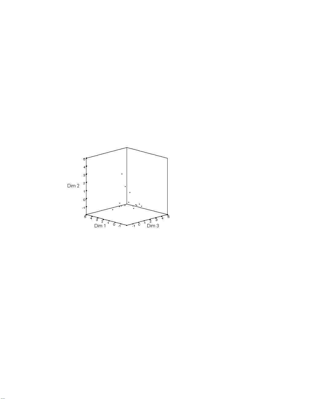
Figure 1.2 shows a three-dimensional plot of object scores produced by a homogeneity
analysis with four dimensions.
Figure 1.2 Three-dimensional plot of object scores
Although only the first three dimensions are displayed on the scatterplot, information
about all dimensions is included when the chart is created. You can choose to display
different combinations of dimensions on the scatterplot by selecting
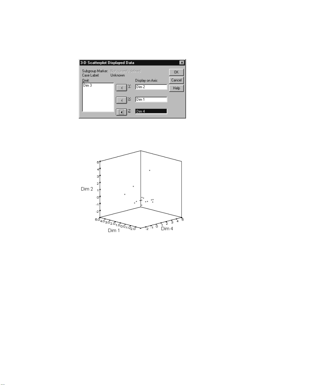
Series menu in the Chart Editor. Figure 1.3 shows the 3-D Scatterplot Displayed Data
dialog box, with dimension 4 selected to be displayed in place of dimension 3. The plot
displaying these selections is shown in Figure 1.4.
Displayed from the
Page 27
Introduction to SPSS Optimal Scaling Procedures for Categorical Data 15
Figure 1.3 3-D Scatterplot Displayed Data dialog box
Figure 1.4 Three-dimensional plot of object scores, displaying dimensions 1, 2, and 4
Scatterplot Matrices
To view more than three dimensions on a single plot, it is useful to graphically display
two-dimensional scatterplots for all dimensions in a matrix scatterplot. To convert a
chart into a scatterplot matrix, use the scatterplot gallery in the Chart Editor. This option
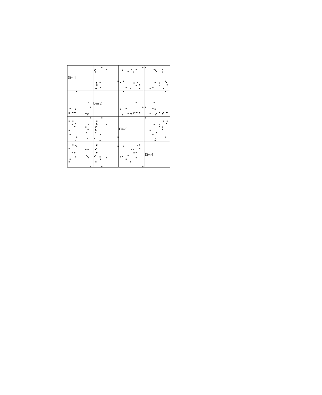
offers great flexibility in converting one chart type to another. A scatterplot matrix displaying four dimensions is shown in Figure 1.5.
Page 28
16 Chapter 1
Figure 1.5 Scatterplot matrix displaying object scores for four dimensions
In contrast to the other dimension reduction techniques, correspondence analysis produces a matrix of scatterplots similar to Figure 1.5 for all analyses. If you desire individual two- or three-dimensional scatterplots, use the Scatter option on the Gallery menu in
the Chart Editor. Alternatively, to omit or add dimensions to an existing scatterplot matrix, use the
for information on editing charts and using the chart gallery).
Displayed command on the Series menu (see the SPSS Base User’s Guide
Aspect Ratio in Optimal Scaling Charts
Aspect ratio in optimal scaling plots is isotropic. In a two-dimensional plot, the distance
representing one unit in dimension 1 is equal to the distance representing one unit in dimension 2. If you change the range of a dimension in a two-dimensional plot, the system
changes the size of the other dimension to keep the physical distances equal. Isotropic
aspect ratio cannot be overridden for the optimal scaling procedures.
Page 29

1
2
Categorical Regression (CATREG)
Categorical regression quantifies categorical data by assigning numerical values
to the categories, resulting in an optimal linear regression equation for the transformed variables. Categorical regression is also known by the acronym CATREG,
for categorical regression.
Standard linear regression analysis involves minimizing the sum of squared differences between a response (dependent) variable and a weighted combination of
predictor (independent) variables. Variables are typically quantitative, with (nominal)
categorical data recoded to binary or contrast variables. As a result, categorical variables serve to separate groups of cases, and the technique estimates separate sets of
parameters for each group. The estimated coefficients reflect how changes in the predictors affect the response. Prediction of the response is possible for any combination
of predictor values.
An alternative approach involves regressing the response on the categorical predictor values themselves. Consequently, one coefficient is estimated for each variable.
However, for categorical variables, the category values are arbitrary. Coding the categories in different ways yield different coefficients, making comparisons across
analyses of the same variables difficult.
CATREG extends the standard approach by simultaneously scaling nominal, ordinal, and numerical variables. The procedure quantifies categorical variables such that
the quantifications reflect characteristics of the original categories. The procedure
treats quantified categorical variables in the same way as numerical variables. Using
nonlinear transformations allow variables to be analyzed at a variety of levels to find
the best-fitting model.
Example. Categorical regression could be used to describe how job satisfaction depends on job category, geographic region, and amount of travel. You might find that
high levels of satisfaction correspond to managers and low travel. The resulting regression equation could be used to predict job satisfaction for any combination of the three
independent variables.
Statistics and plots. Frequencies, regression coefficients, ANOVA table, iteration history, category quantifications, correlations between untransformed predictors, correlations between transformed predictors, residual plots, and transformation plots.
17
Page 30
18 Chapter 2
Data. CATREG operates on category indicator variables. The category indicators should
be positive integers. You can use the Discretization dialog box to convert fractional-value variables and string variables into positive integers.
Assumptions. Only one response variable is allowed, but the maximum number of predictor variables is 200. The data must contain at least three valid cases, and the number
of valid cases must exceed the number of predictor variables plus one.
Related procedures. CATREG is equivalent to categorical canonical correlation
analysis with optimal scaling (OVERALS) with two sets, one of which contains only
one variable. Scaling all variables at the numerical level corresponds to standard
multiple regression analysis.
To Obtain a Categorical Regression
From the menus choose:
Analyze
Regression
Optimal Scaling…
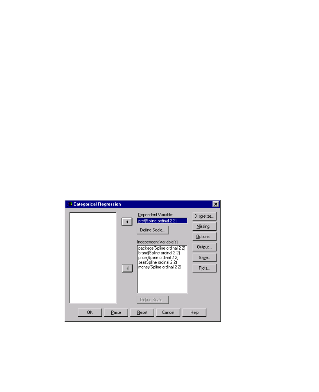
Figure 2.1 Categorical Regression dialog box
Select the dependent variable and independent variable(s).
Click OK.
Optionally, change the scaling level for each variable.
Page 31

Define Scale in Categorical Regression
You can set the optimal scaling level for the dependent and independent variables. By
default, they are scaled as second-degree monotonic splines (ordinal) with two interior
knots. Additionally, you can set the weight for analysis variables.
Optimal Scaling Level. You can also select the scaling level for quantifying each
variable.
• Spline Ordinal. The order of the categories of the observed variable is preserved in
the optimally scaled variable. Category points will be on a straight line (vector)
through the origin. The resulting transformation is a smooth monotonic piecewise
polynomial of the chosen degree. The pieces are specified by the user-specified number and procedure-determined placement of the interior knots.
• Spline Nominal. The only information in the observed variable that is preserved in
the optimally scaled variable is the grouping of objects in categories. The order of the
categories of the observed variable is not preserved. Category points will be on a
straight line (vector) through the origin. The resulting transformation is a smooth,
possibly nonmonotonic, piecewise polynomial of the chosen degree. The pieces are
specified by the user-specified number and procedure-determined placement of the
interior knots.
• Ordinal. The order of the categories of the observed variable is preserved in the opti-
mally scaled variable. Category points will be on a straight line (vector) through the
origin. The resulting transformation fits better than the spline ordinal transformation
but is less smooth.
• Nominal. The only information in the observed variable that is preserved in the opti-
mally scaled variable is the grouping of objects in categories. The order of the categories of the observed variable is not preserved. Category points will be on a straight
line (vector) through the origin. The resulting transformation fits better than the
spline nominal transformation but is less smooth.
• Numeric. Categories are treated as ordered and equally spaced (interval level). The
order of the categories and the equal distances between category numbers of the observed variable are preserved in the optimally scaled variable. Category points will
be on a straight line (vector) through the origin. When all variables are at the numeric
level, the analysis is analogous to standard principal components analysis.
Categorical Regression (CATREG) 19
Page 32
20 Chapter 2
To Define the Scale in CATREG
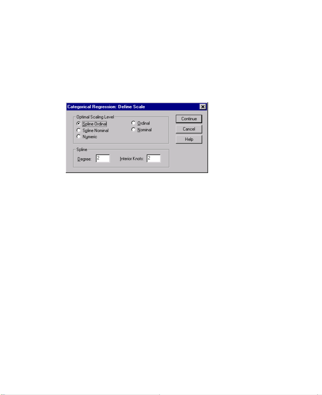
Select one or more variables on the variables list in the Categorical Regression dialog box.
Click Define Scale.
Figure 2.2 Categorical Regression Define Scale dialog box
Select the optimal scaling level to be used in the analysis.
Click Continue.
Categorical Regression Discretization
The Discretization dialog box allows you to select a method of recoding your variables.
Fractional-value variables are grouped into seven categories (or into the number of distinct values of the variable, if this number is less than seven) with an approximately normal distribution, unless specified otherwise. String variables are always converted into
positive integers by assigning category indicators according to ascending alphanumeric
order. Discretization for string variables applies to these integers. Other variables are left
alone by default. The discretized variables are then used in the analysis.
Page 33
Categorical Regression (CATREG) 21
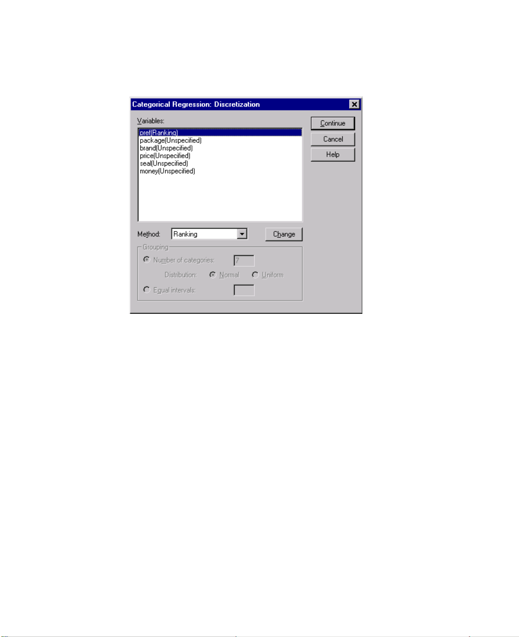
Figure 2.3 Categorical Regression Discretization dialog box
Method. Choose between grouping, ranking, or multiplying.
• Grouping. Recode into a specified number of categories or recode by interval.
• Ranking. The variable is discretized by ranking the cases.
• Multiplying. The current values of the variable are standardized, multiplied by 10,
rounded, and have a constant added such that the lowest discretized value is 1.
Grouping. The following options are available when discretizing variables by grouping:
• Number of categories. Specify a number of categories and whether the values of the
variable should follow an approximately normal or uniform distribution across those
categories.
• Equal intervals. Variables are recoded into categories defined by these equally sized
intervals. You must specify the length of the intervals.
Page 34
22 Chapter 2
Categorical Regression Missing Values
The Missing Values dialog box allows you to choose the strategy for handling missing
values in analysis variables and supplementary variables.
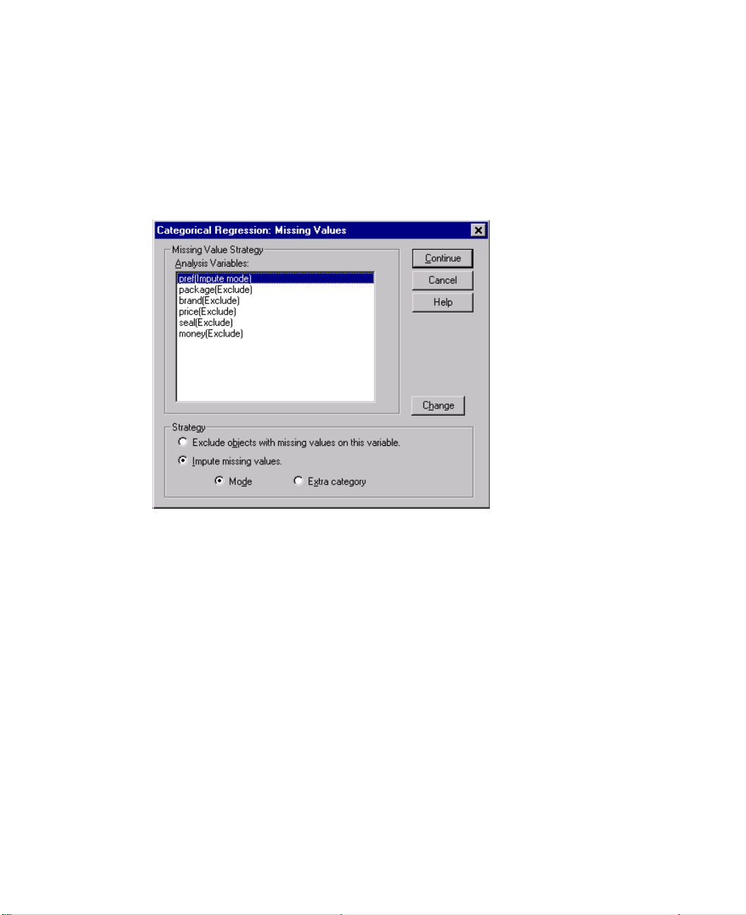
Figure 2.4 Categorical Regression Missing Values dialog box
Strategy. Choose to impute missing values (active treatment) or exclude objects with
missing values (listwise deletion).
• Impute missing values. Objects with missing values on the selected variable have
those values imputed. You can choose the method of imputation. Select
Mode to re-
place missing values with the most frequent category. When there are multiple
modes, the one with the smallest category indicator is used. Select
Extra category to
replace missing values with the same quantification of an extra category. This implies that objects with a missing value on this variable are considered to belong to the
same (extra) category.
• Exclude objects with missing values on this variable. Objects with missing values
on the selected variable are excluded from the analysis. This strategy is not available
for supplementary variables.
Page 35
Categorical Regression Options
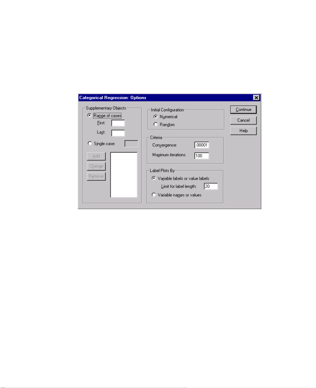
The Options dialog box allows you to select the initial configuration style, specify iteration
and convergence criteria, select supplementary objects, and set the labeling of plots.
Figure 2.5 Categorical Regression Options dialog box
Categorical Regression (CATREG) 23
Supplementary Objects. This allows you to specify the objects that you want to treat as
supplementary. Simply type the number of a supplementary object and click
Add. You
cannot weight supplementary objects (specified weights are ignored).
Initial Configuration. If no variables are treated as nominal, select the
uration. If at least one variable is treated as nominal, select the
Numerical config-
Random configuration.
Criteria. You can specify the maximum number of iterations the regression may go
through in its computations. You can also select a convergence criterion value. The regression stops iterating if the difference in total fit between the last two iterations is less
than the convergence value or if the maximum number of iterations is reached.
Label Plots By. Allows you to specify whether variables and value labels or variable names
and values will be used in the plots. You can also specify a maximum length for labels.
Page 36
24 Chapter 2
Categorical Regression Ou tput
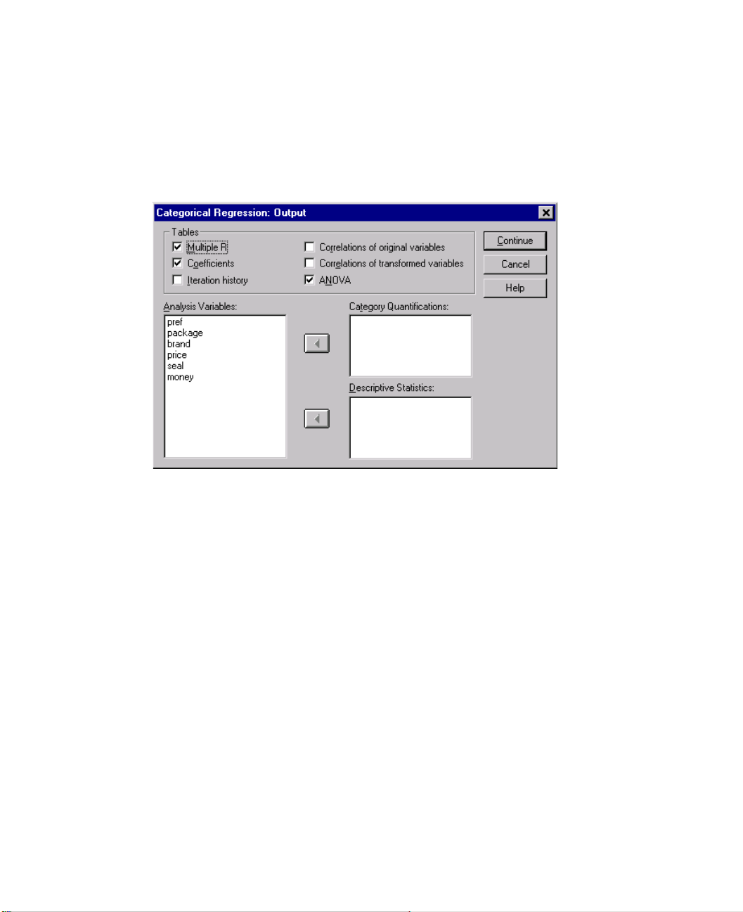
The Output dialog box allows you to select the statistics to display in the output.
Figure 2.6 Categorical Regression Output dialog box
Tab le s. Produces tables for:
2
• Multiple R. Includes R
, adjusted R2, and adjusted R2 taking the optimal scaling into
account.
• Coefficients. This option gives three tables: a Coefficients table that includes betas,
standard error of the betas, t values, and significance; a Coefficients-Optimal Scaling
table with the standard error of the betas taking the optimal scaling degrees of freedom into account; and a table with the zero-order, part, and partial correlation, Pratt’s
relative importance measure for the transformed predictors, and the tolerance before
and after transformation.
• Iteration history. For each iteration, including the starting values for the algorithm,
the multiple R and regression error are shown. The increase in multiple R is listed
starting from the first iteration.
• Correlations of the original variables. A matrix showing the correlations between the
untransformed variables is displayed.
• Correlations of the transformed variables. A matrix showing the correlations
between the transformed variables is displayed.
Page 37
• ANOVA. This option includes regression and residual sums of squares, mean squares,
and F. Two ANOVA tables are displayed: one with degrees of freedom for the
regression equal to the number of predictor variables and one with degrees of freedom for the regression taking the optimal scaling into account.
Category Quantifications. Tables showing the transformed values of the selected
variables are displayed.
Descriptive Statistics. Tables showing the frequencies, missing values, and modes of
the selected variables are displayed.
Categorical Regression Save
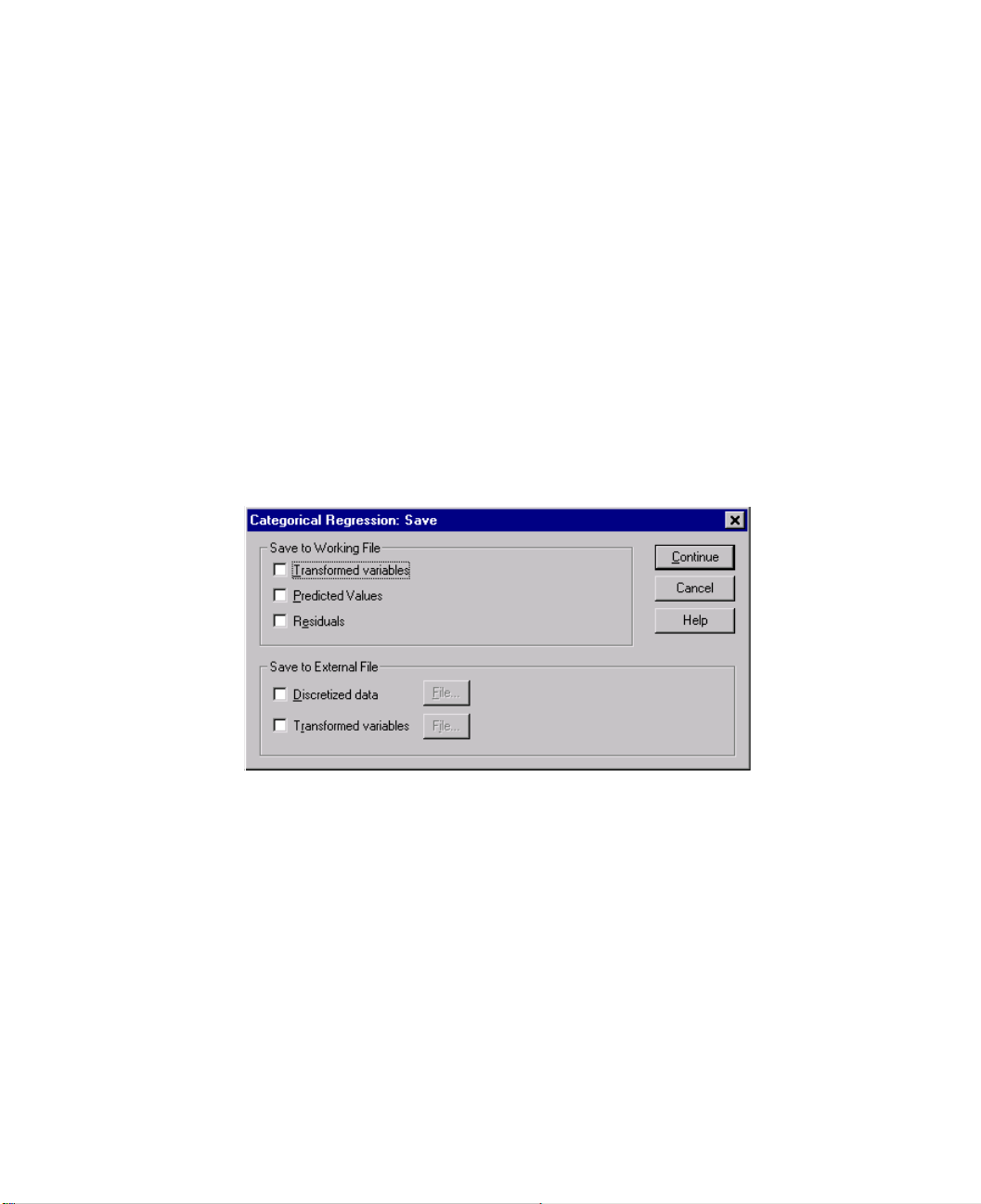
The Save dialog box allows you to save results to the working file or an external file.
Figure 2.7 Categorical Regression Save dialog box
Categorical Regression (CATREG) 25
Save to Working File. You can save the transformed values of the variables, modelpredicted values, and residuals to the working file.
Save to External File. You can save the discretized data and transformed variables to
external files.
Page 38
26 Chapter 2
Categorical Regression Plots
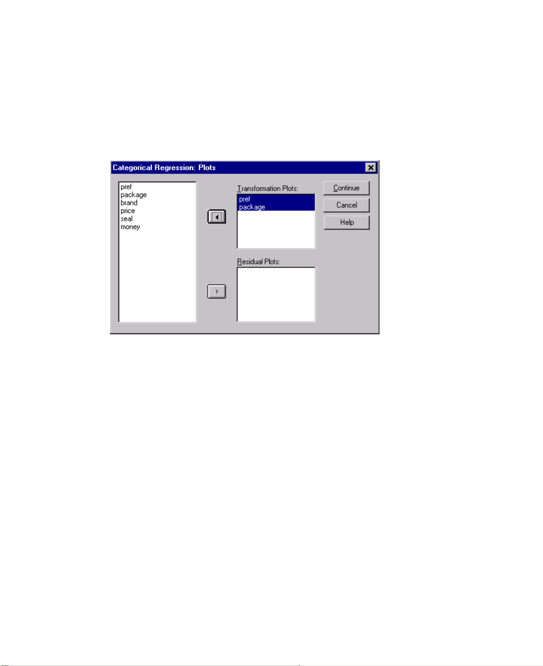
The Plot dialog box allows you to specify the variables that will produce transformation
and residual plots.
Figure 2.8 Categorical Regression Plot dialog box
Transformation Plots. For each of these variables, the category quantifications are plotted against the original category values. Empty categories appear on the horizontal axis
but do not affect the computations. These categories are identified by breaks in the line
connecting the quantifications.
Residual Plots. For each of these variables, residuals (computed for the dependent variable predicted from all predictor variables except the predictor variable in question) are
plotted against category indicators and the optimal category quantifications multiplied
with beta against category indicators.
CATREG Command Additional Features
You can customize your categorical regression if you paste your selections into a syntax
window and edit the resulting
also allows you to:
• Specify rootnames for the transformed variables when saving them to the working
data file (with the
SAVE subcommand).
CATREG command syntax. SPSS command language
Page 39

3
Categorical Principal Components Analysis (CATPCA)
This procedure simultaneously quantifies categorical variables while reducing the dimensionality of the data. Categorical principal components analysis is also known by
the acronym CATPCA, for categorical principal components analysis.
The goal of principal components analysis is to reduce an original set of variables
into a smaller set of uncorrelated components that represent most of the information
found in the original variables. The technique is most useful when a large number of
variables prohibits effective interpretation of the relationships between objects (subjects and units). By reducing the dimensionality, you interpret a few components rather
than a large number of variables.
Standard principal components analysis assumes linear relationships between
numeric variables. On the other hand, the optimal-scaling approach allows variables to
be scaled at different levels. Categorical variables are optimally quantified in the specified dimensionality. As a result, nonlinear relationships between variables can be
modeled.
Example. Categorical principal components analysis could be used to graphically display the relationship between job category, job division, region, amount of travel (high,
medium, and low), and job satisfaction. You might find that two dimensions account for
a large amount of variance. The first dimension might separate job category from region,
whereas the second dimension might separate job division from amount of travel. You
also might find that high job satisfaction is related to a medium amount of travel.
Statistics and plots. Frequencies, missing values, optimal scaling level, mode, variance
accounted for by centroid coordinates, vector coordinates, total per variable and per dimension, component loadings for vector-quantified variables, category quantifications
and coordinates, iteration history, correlations of the transformed variables and eigenvalues of the correlation matrix, correlations of the original variables and eigenvalues
of the correlation matrix, object scores, category plots, joint category plots, transformation plots, residual plots, projected centroid plots, object plots, biplots, triplots, and
component loadings plots.
Data. String variable values are always converted into positive integers by ascending
alphanumeric order. User-defined missing values, system-missing values, and values
less than 1 are considered missing; you can recode or add a constant to variables with
values less than 1 to make them nonmissing.
27
Page 40
28 Chapter 3
Assumptions. The data must contain at least three valid cases. The analysis is based on
positive integer data. The discretization option will automatically categorize a fractionalvalue variable by grouping its values into categories with a close to “normal” distribution
and will automatically convert values of string variables into positive integers. You can
specify other discretization schemes.
Related procedures. Scaling all variables at the numeric level corresponds to standard
principal components analysis. Alternate plotting features are available by using the
transformed variables in a standard linear principal components analysis. If all variables
have multiple nominal scaling levels, categorical principal components analysis is identical to homogeneity analysis. If sets of variables are of interest, categorical (nonlinear)
canonical correlation analysis should be used.
To Obtain a Categorical Principal Components Analysis
From the menus choose:
Analyze
Data Reduction
Optimal Scaling...
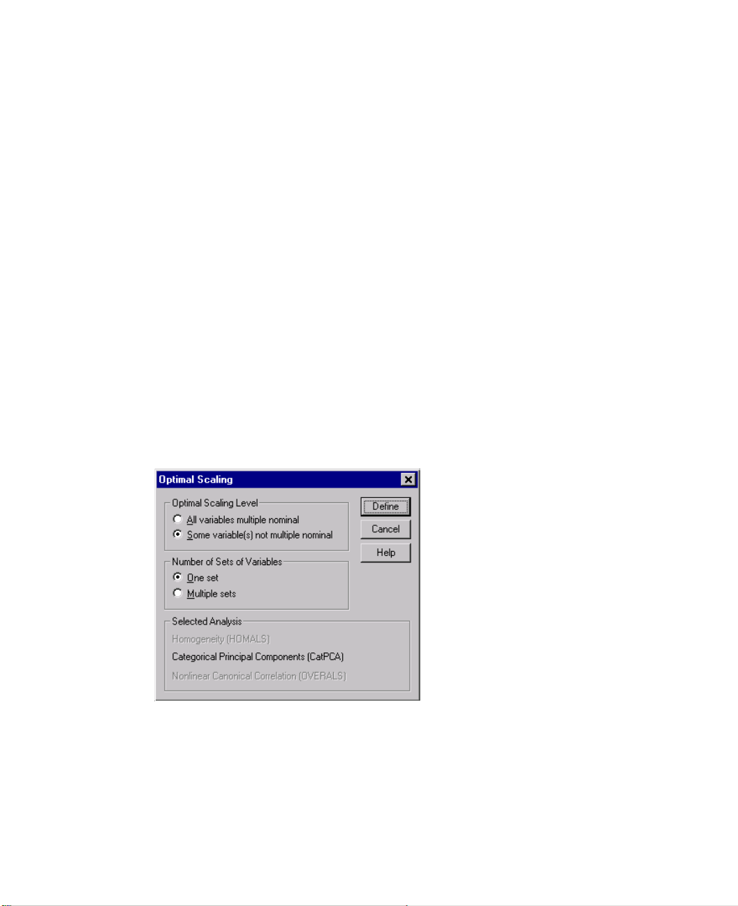
Figure 3.1 Optimal Scaling dialog box
Select Some variable(s) not multiple nominal.
Select One set.
Click Define.
Page 41
Categorical Principal Components Analysis (CATPCA) 29
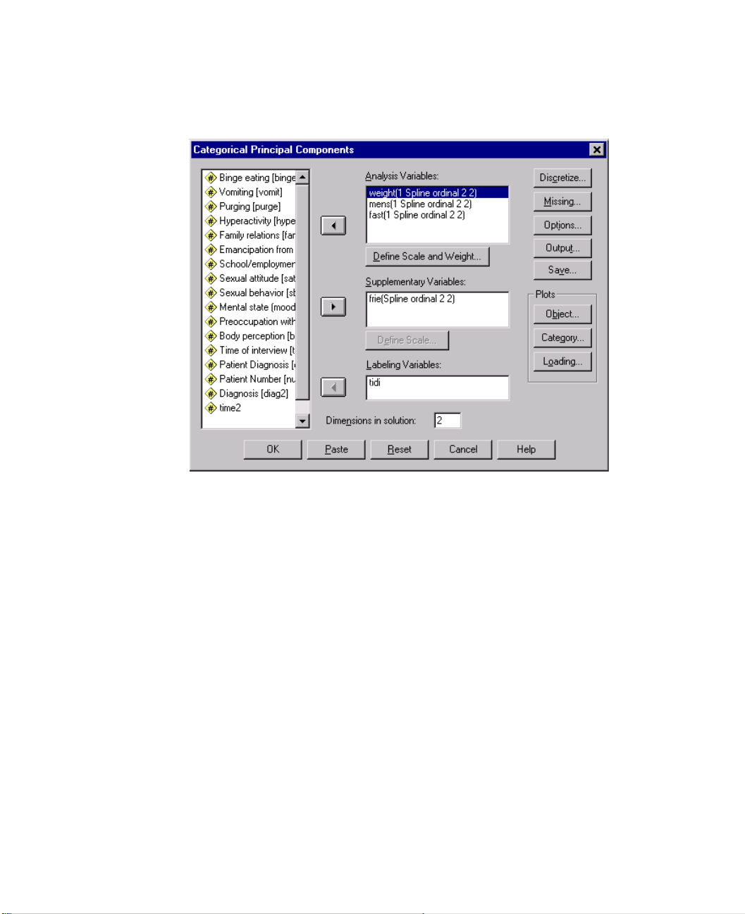
Figure 3.2 Categorical Principal Components dialog box
Select at least two analysis variables and specify the number of dimensions in the
solution.
Click OK.
You may optionally specify supplementary variables, which are fitted into the solution
found, or labeling variables for the plots.
Define Scale and Weight in CATPCA
You can set the optimal scaling level for analysis variables and supplementary variables.
By default, they are scaled as second-degree monotonic splines (ordinal) with two interior knots. Additionally, you can set the weight for analysis variables.
Variable weight.
fied must be a positive integer. The default value is 1.
Optimal Scaling Level. You can also select the scaling level to be used to quantify each
variable.
You can choose to define a weight for each variable. The value speci-
Page 42

30 Chapter 3
• Spline ordinal. The order of the categories of the observed variable is preserved in
the optimally scaled variable. Category points will be on a straight line (vector)
through the origin. The resulting transformation is a smooth monotonic piecewise
polynomial of the chosen degree. The pieces are specified by the user-specified number and procedure-determined placement of the interior knots.
• Spline nominal. The only information in the observed variable that is preserved in the
optimally scaled variable is the grouping of objects in categories. The order of the
categories of the observed variable is not preserved. Category points will be on a
straight line (vector) through the origin. The resulting transformation is a smooth,
possibly nonmonotonic, piecewise polynomial of the chosen degree. The pieces are
specified by the user-specified number and procedure-determined placement of the
interior knots.
• Multiple nominal. The only information in the observed variable that is preserved in
the optimally scaled variable is the grouping of objects in categories. The order of the
categories of the observed variable is not preserved. Category points will be in the
centroid of the objects in the particular categories. Multiple indicates that different
sets of quantifications are obtained for each dimension.
• Ordinal. The order of the categories of the observed variable is preserved in the opti-
mally scaled variable. Category points will be on a straight line (vector) through the
origin. The resulting transformation fits better than the spline ordinal transformation
but is less smooth.
• Nominal. The only information in the observed variable that is preserved in the opti-
mally scaled variable is the grouping of objects in categories. The order of the categories of the observed variable is not preserved. Category points will be on a straight
line (vector) through the origin. The resulting transformation fits better than the
spline nominal transformation but is less smooth.
• Numeric. Categories are treated as ordered and equally spaced (interval level). The
order of the categories and the equal distances between category numbers of the observed variable are preserved in the optimally scaled variable. Category points will
be on a straight line (vector) through the origin. When all variables are at the numeric
level, the analysis is analogous to standard principal components analysis.
Page 43
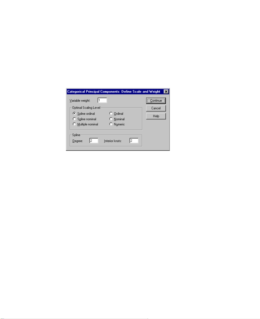
Categorical Principal Components Analysis (CATPCA) 31
To Define the Scale and Weight in CATPCA
Select a variable in the Analysis Variables list in the Categorical Principal Components
dialog box.
Click Define Scale and Weight.
Figure 3.3 Categorical Principal Components Define Scale and Weight dialog box
Enter the weight value for the variable.
Select the optimal scaling level to be used in the analysis. If you choose a spline trans-
formation, you must also specify the degree of the polynomial and the number of interior
knots.
Click Continue.
You can alternatively define the scaling level for supplementary variables by selecting
them from the list and clicking
Define Scale.
Page 44
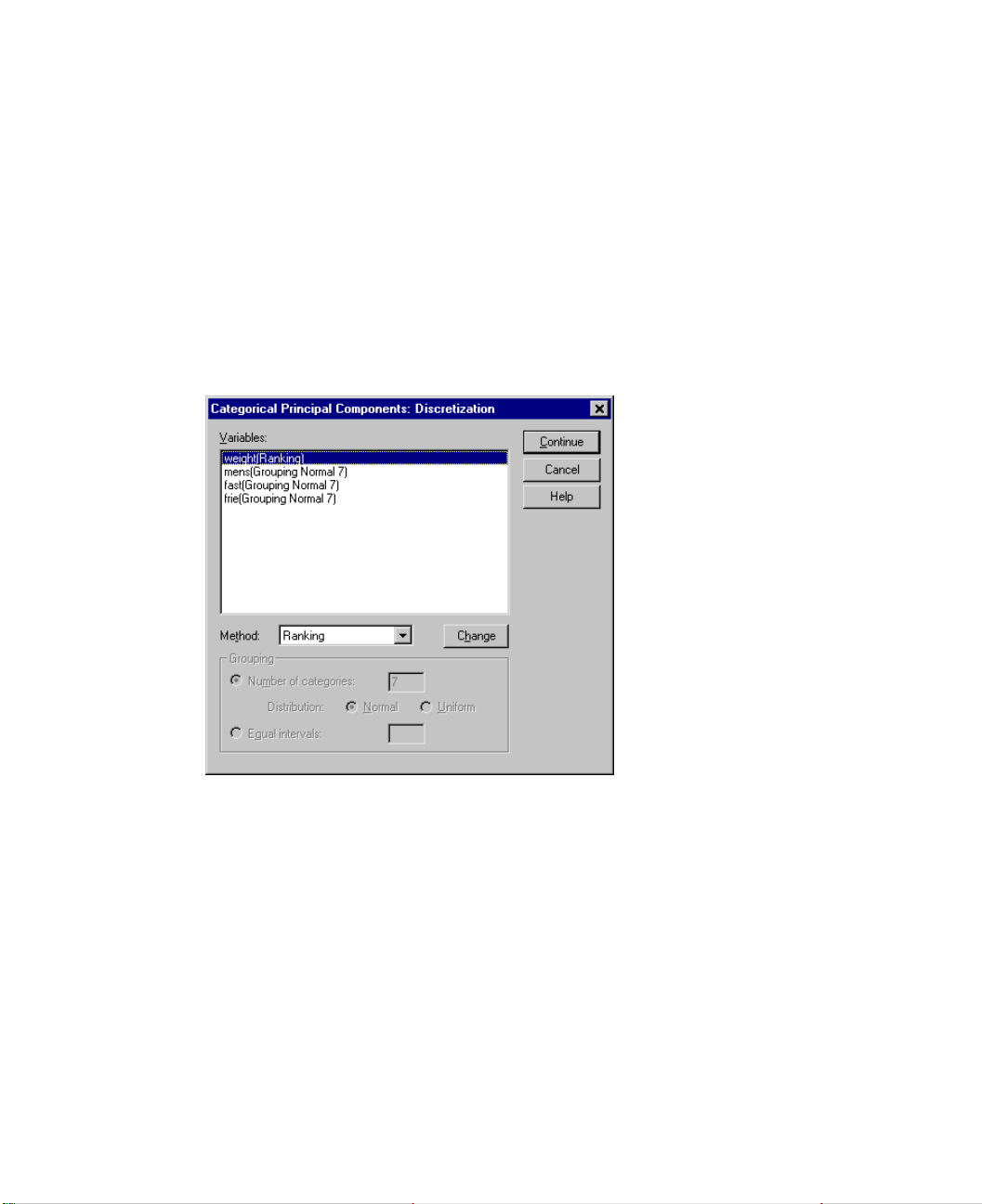
32 Chapter 3
Categorical Principal Components Discretization
The Discretization dialog box allows you to select a method of recoding your variables.
Fractional-value variables are grouped into seven categories (or into the number of distinct values of the variable if this number is less than seven) with an approximately normal distribution, unless specified otherwise. String variables are always converted into
positive integers by assigning category indicators according to ascending alphanumeric
order. Discretization for string variables applies to these integers. Other variables are left
alone by default. The discretized variables are then used in the analysis.
Figure 3.4 Categorical Principal Components Discretization dialog box
Method. Choose between grouping, ranking, and multiplying.
• Grouping. Recode into a specified number of categories or recode by interval.
• Ranking. The variable is discretized by ranking the cases.
• Multiplying. The current values of the variable are standardized, multiplied by 10,
rounded, and have a constant added such that the lowest discretized value is 1.
Grouping. The following options are available when discretizing variables by grouping:
• Number of categories. Specify a number of categories and whether the values of the
variable should follow an approximately normal or uniform distribution across those
categories.
• Equal intervals. Variables are recoded into categories defined by these equally sized
intervals. You must specify the length of the intervals.
Page 45
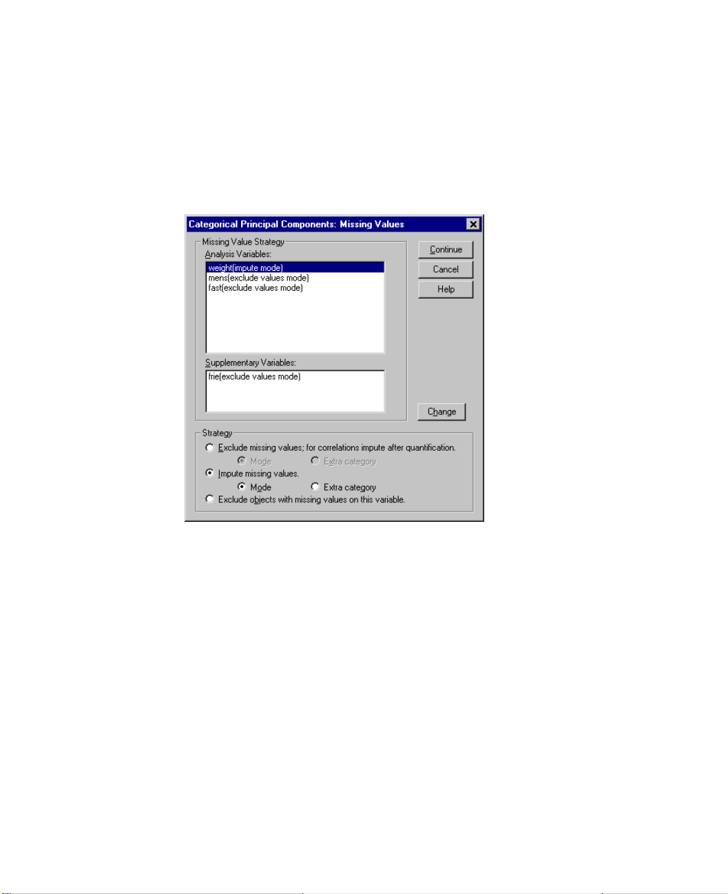
Categorical Principal Components Analysis (CATPCA) 33
Categorical Principal Components Missing Values
The Missing Values dialog box allows you to choose the strategy for handling missing
values in analysis variables and supplementary variables.
Figure 3.5 Categorical Principal Components Missing Values dialog box
Strategy. Choose to exclude missing values (passive treatment), impute missing values
(active treatment), or exclude objects with missing values (listwise deletion).
• Exclude missing values; for correlations impute after quantification. Objects with
missing values on the selected variable do not contribute to the analysis for this variable. If all variables are given passive treatment, then objects with missing values on
all variables are treated as supplementary. If correlations are specified in the Output
dialog box, then (after analysis) missing values are imputed with the most frequent
category, or mode, of the variable for the correlations of the original variables. For
the correlations of the optimally scaled variables, you can choose the method of imputation. Select
scaled variable. Select
Mode to replace missing values with the mode of the optimally
Extra category to replace missing values with the quantifica-
tion of an extra category. This implies that objects with a missing value on this variable are considered to belong to the same (extra) category.
Page 46
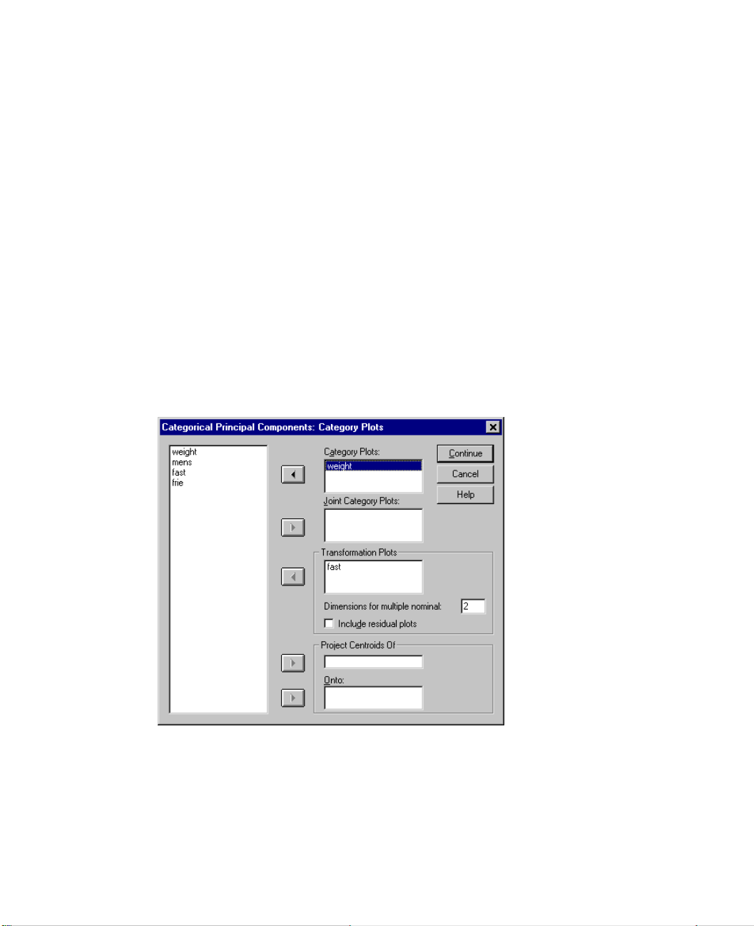
34 Chapter 3
• Impute missing values. Objects with missing values on the selected variable have
those values imputed. You can choose the method of imputation. Select
place missing values with the most frequent category. When there are multiple
modes, the one with the smallest category indicator is used. Select
replace missing values with the same quantification of an extra category. This implies that objects with a missing value on this variable are considered to belong to the
same (extra) category.
• Exclude objects with missing values on this variable. Objects with missing values
on the selected variable are excluded from the analysis. This strategy is not available
for supplementary variables.
Categorical Principal Components Category Plots
The Category Plots dialog box allows you to specify the types of plots desired and the
variables for which plots will be produced.
Figure 3.6 Categorical Principal Components Category Plots dialog box
Mode to re-
Extra category to
Category Plots. For each variable selected, a plot of the centroid and vector coordinates
is plotted. For variables with multiple nominal scaling levels, categories are in the centroids of the objects in the particular categories. For all other scaling levels, categories
are on a vector through the origin.
Page 47
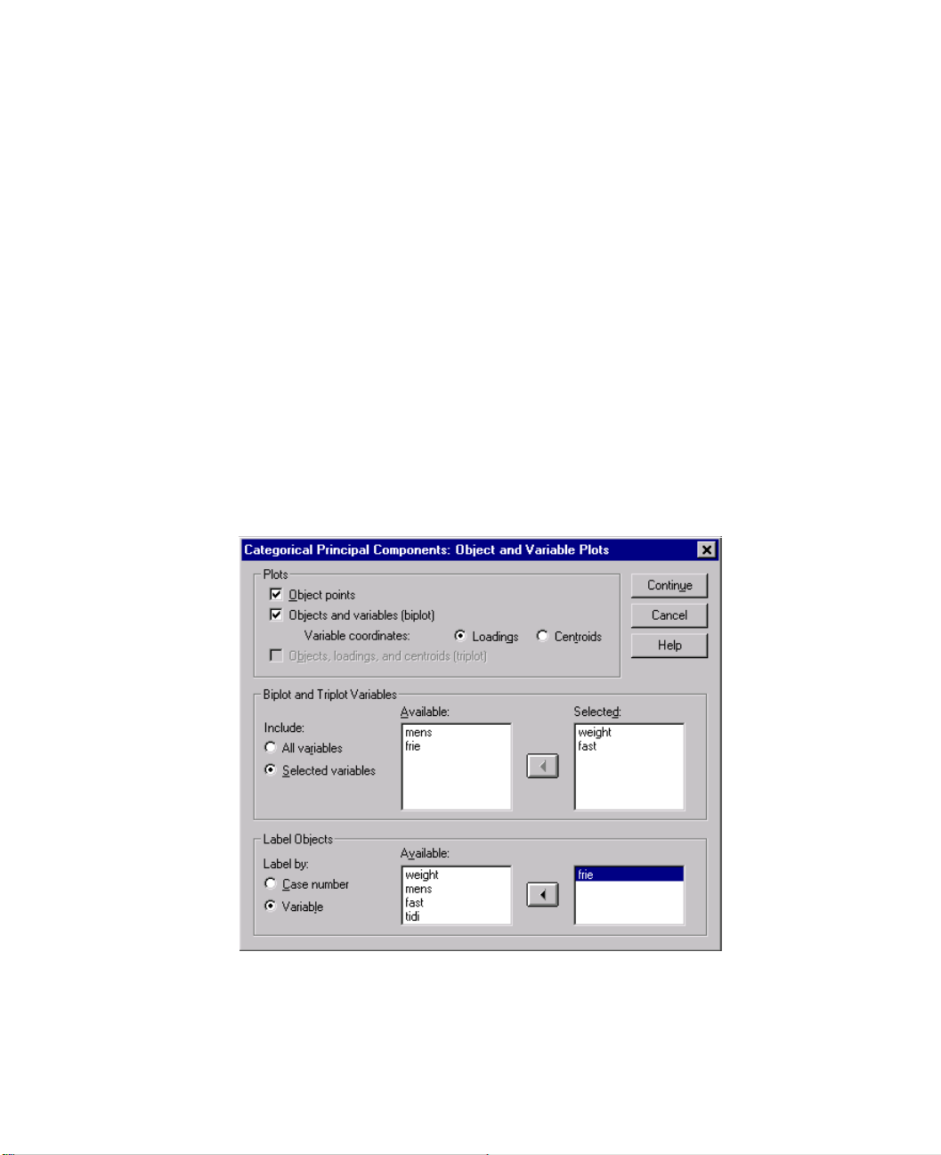
Categorical Principal Components Analysis (CATPCA) 35
Joint Category Plots. This is a single plot of the centroid and vector coordinates of each
selected variable.
Transformation Plots. Displays a plot of the optimal category quantifications versus the
category indicators. You can specify the number of dimensions desired for variables
with multiple nominal scaling levels; one plot will be generated for each dimension. You
can also choose to display residual plots for each variable selected.
Project Centroids Of. You may choose a variable and project its centroids onto selected
variables. Variables with multiple nominal scaling levels cannot be selected to project
on. When this plot is requested, a table with the coordinates of the projected centroids is
also displayed.
Categorical Principal Components Object and Variable Plots
The Object and Variable Plots dialog box allows you to specify the types of plots desired
and the variables for which plots will be produced.
Figure 3.7 Categorical Principal Components Object and Variable Plots dialog box
Page 48
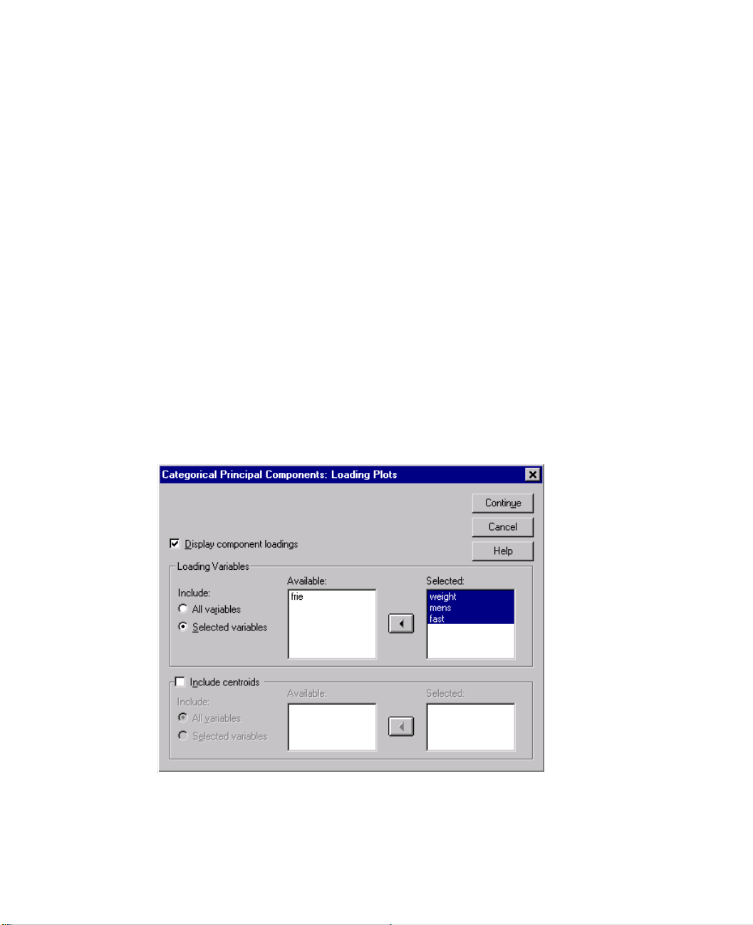
36 Chapter 3
Object points. A plot of the object points is displayed.
Objects and variables (biplot). The object points are plotted with your choice of the vari-
able coordinates—component loadings or variable centroids.
Objects, loadings, and centroids (triplot). The object points are plotted with the centroids of multiple nominal-scaling-level variables and the component loadings of other
variables.
Biplot and Triplot Variables. You can choose to use all variables for the biplots and
triplots, or select a subset.
Label Objects. You can choose to have objects labeled with the categories of selected
variables (you may choose category indicator values or value labels in the Options dialog
box) or with their case numbers. One plot is produced per variable, if
Categorical Principal Components Loading Plots
The Loading Plots dialog box allows you to specify the variables which will be included
in the plot, and whether or not to include centroids in the plot.
Figure 3.8 Categorical Principal Components Loading Plots dialog box
Var iable is selected.
Display component loadings. If selected, a plot of the component loadings is displayed.
Loading Variables. You can choose to use all variables for the component loadings plot
or select a subset.
Page 49
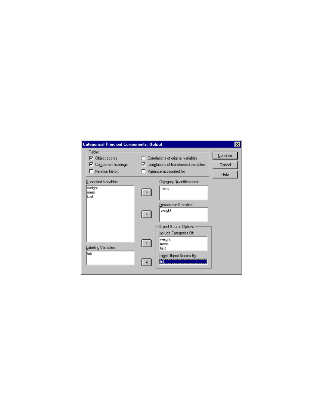
Include centroids. Variables with multiple nominal scaling levels do not have component loadings, but you may choose to include the centroids of those variables in the plot.
You can choose to use all multiple nominal variables or select a subset.
Categorical Principal Components Output
The Output dialog box allows you to produce tables for object scores, component loadings, iteration history, correlations of original and transformed variables, the variance
accounted for per variable and per dimension, category quantifications for selected variables, and descriptive statistics for selected variables.
Figure 3.9 Categorical Principal Components Output dialog box
Categorical Principal Components Analysis (CATPCA) 37
Object scores. Displays the object scores and has the following options:
• Include Categories Of. Displays the category indicators of the analysis variables
selected.
• Label Object Scores By. From the list of variables specified as labeling variables, you
can select one to label the objects.
Component loadings. Displays the component loadings for all variables that were not
given multiple nominal scaling levels.
Page 50
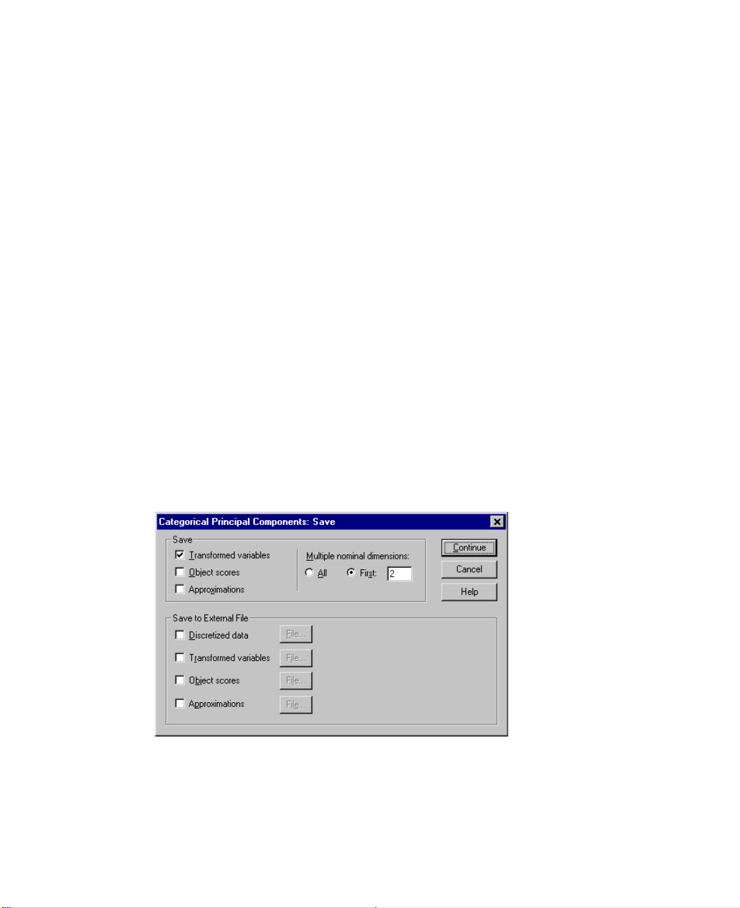
38 Chapter 3
Iteration history. For each iteration, the variance accounted for, loss, and increase in
variance accounted for are shown.
Correlations of original variables. Shows the correlation matrix of the original variables
and the eigenvalues of that matrix.
Correlations of transformed variables. Shows the correlation matrix of the transformed
(optimally scaled) variables and the eigenvalues of that matrix.
Variance accounted for. Displays the amount of variance accounted for by centroid coordinates, vector coordinates, and total (centroid and vector coordinates combined) per
variable and per dimension.
Category Quantifications. Gives the category quantifications and coordinates for each
dimension of the variable(s) selected.
Descriptive Statistics. Displays frequencies, number of missing values, and mode of the
variable(s) selected.
Categorical Principal Components Save
The Save dialog box allows you to add the transformed variables, object scores, and approximations to the working data file or as new variables in external files and save the
discretized data as new variables in an external data file.
Figure 3.10 Categorical Principal Components Save dialog box
Save. Save selections to the working data file. If any variable has been given the multiple nominal scaling level, the number of dimensions to be saved must be specified.
Save to External File. Save selections to a new external file. Specify a filename for each
selected option by clicking
File. Each file specified must have a different name.
Page 51
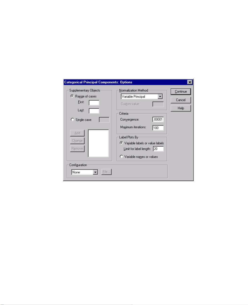
Categorical Principal Components Analysis (CATPCA) 39
Categorical Principal Components Options
The Options dialog box allows you to select the initial configuration, specify iteration
and convergence criteria, select a normalization method, choose the method for labeling
plots, and specify supplementary objects.
Figure 3.11 Categorical Principal Components Options dialog box
Supplementary Objects. Specify the case number of the object, or the first and last case
numbers of a range of objects, that you want to make supplementary and then click
Continue until you have specified all of your supplementary objects. If an object is specified as supplementary, then case weights are ignored for that object.
Normalization Method. You can specify one of five options for normalizing the object
scores and the variables. Only one normalization method can be used in a given analysis.
• Variable Principal. This option optimizes the association between variables. The co-
ordinates of the variables in the object space are the component loadings (correlations
with principal components, such as dimensions and object scores). This is useful
when you are primarily interested in the correlation between the variables.
• Object Principal. This option optimizes distances between objects. This is useful
when you are primarily interested in differences or similarities between the objects.
• Symmetrical. Use this normalization option if you are primarily interested in the re-
lation between objects and variables.
Add.
Page 52

40 Chapter 3
• Independent. Use this normalization option if you want to examine distances be-
tween objects and correlations between variables separately.
• Custom. You can specify any real value in the closed interval [–1, 1]. A value of 1 is
equal to the Object Principal method, a value of 0 is equal to the Symmetrical method, and a value of –1 is equal to the Variable Principal method. By specifying a value
greater than –1 and less than 1, you can spread the eigenvalue over both objects and
variables. This method is useful for making a tailor-made biplot or triplot.
Criteria. You can specify the maximum number of iterations the procedure can go
through in its computations. You can also select a convergence criterion value. The algorithm stops iterating if the difference in total fit between the last two iterations is less
than the convergence value or if the maximum number of iterations is reached.
Configuration. You can read data from a file containing the coordinates of a configuration. The first variable in the file should contain the coordinates for the first dimension,
the second variable should contain the coordinates for the second dimension, and so on.
• Initial. The configuration in the file specified will be used as the starting point of the
analysis.
• Fixed. The configuration in the file specified will be used to fit in the variables. The
variables that are fitted in must be selected as analysis variables, but because the configuration is fixed, they are treated as supplementary variables (so they do not need
to be selected as supplementary variables).
Label Plots By. Allows you to specify whether variables and value labels or variable
names and values will be used in the plots. You can also specify a maximum length for
labels.
CATPCA Command Add itional Features
You can customize your categorical principal components analysis if you paste your selections into a syntax window and edit the resulting
command language also allows you to:
• Specify rootnames for the transformed variables, object scores, and approximations
when saving them to the working data file (with the
• Specify a maximum length for labels for each plot separately (with the
subcommand).
• Specify a separate variable list for residual plots (with the
CATPCA command syntax. SPSS
SAVE subcommand).
PLOT
PLOT subcommand).
Page 53

4
Nonlinear Canonical Correlation Analysis (OVERALS)
Nonlinear canonical correlation analysis corresponds to categorical canonical correlation analysis with optimal scaling. The purpose of this procedure is to determine how
similar sets of categorical variables are to one another. Nonlinear canonical correlation
analysis is also known by the acronym OVERALS.
Standard canonical correlation analysis is an extension of multiple regression,
where the second set does not contain a single response variable, but multiple ones. The
goal is to explain as much as possible of the variance in the relationships among two
sets of numerical variables in a low dimensional space. Initially, the variables in each
set are linearly combined such that the linear combinations have a maximal correlation.
Given these combinations, subsequent linear combinations are determined that are
uncorrelated with the previous combinations and that have the largest correlation
possible.
The optimal scaling approach expands the standard analysis in three crucial ways.
First, OVERALS allows more than two sets of variables. Second, variables can be
scaled as either nominal, ordinal, or numerical. As a result, nonlinear relationships
between variables can be analyzed. Finally, instead of maximizing correlations
between the variable sets, the sets are compared to an unknown compromise set defined
by the object scores.
Example. Categorical canonical correlation analysis with optimal scaling could be used
to graphically display the relationship between one set of variables containing job category and years of education and another set of variables containing minority classification and gender. You might find that years of education and minority classification
discriminate better than the remaining variables. You might also find that years of education discriminates best on the first dimension.
Statistics and plots. Frequencies, centroids, iteration history, object scores, category
quantifications, weights, component loadings, single and multiple fit, object scores
plots, category coordinates plots, component loadings plots, category centroids plots,
transformation plots.
Data. Use integers to code categorical variables (nominal or ordinal scaling level). To
minimize output, use consecutive integers beginning with 1 to code each variable. Variables scaled at the numerical level should not be recoded to consecutive integers. To
41
Page 54

42 Chapter 4
minimize output, for each variable scaled at the numerical level, subtract the smallest
observed value from every value and add 1. Fractional values are truncated after the
decimal.
Assumptions. Variables can be classified into two or more sets. Variables in the analysis
are scaled as multiple nominal, single nominal, ordinal, or numerical. The maximum
number of dimensions used in the procedure depends on the optimal scaling level of the
variables. If all variables are specified as ordinal, single nominal, or numerical, the maximum number of dimensions is the minimum of the number of observations minus 1 and
the total number of variables. However, if only two sets of variables are defined, the
maximum number of dimensions is the number of variables in the smaller set. If some
variables are multiple nominal, the maximum number of dimensions is the total number
of multiple nominal categories plus the number of nonmultiple nominal variables minus
the number of multiple nominal variables. For example, if the analysis involves five
variables, one of which is multiple nominal with four categories, the maximum number
of dimensions is (4 + 4 – 1), or 7. If you specify a number greater than the maximum,
the maximum value is used.
Related procedures. If each set contains one variable, nonlinear canonical correlation
analysis is equivalent to principal components analysis with optimal scaling. If each of
these variables is multiple nominal, the analysis corresponds to homogeneity analysis.
If two sets of variables are involved and one of the sets contains only one variable, the
analysis is identical to categorical regression with optimal scaling.
To Obtain a Nonlinear Canonical Correlation Analysis
From the menus choose:
Analyze
Data Reduction
Optimal Scaling...
Page 55
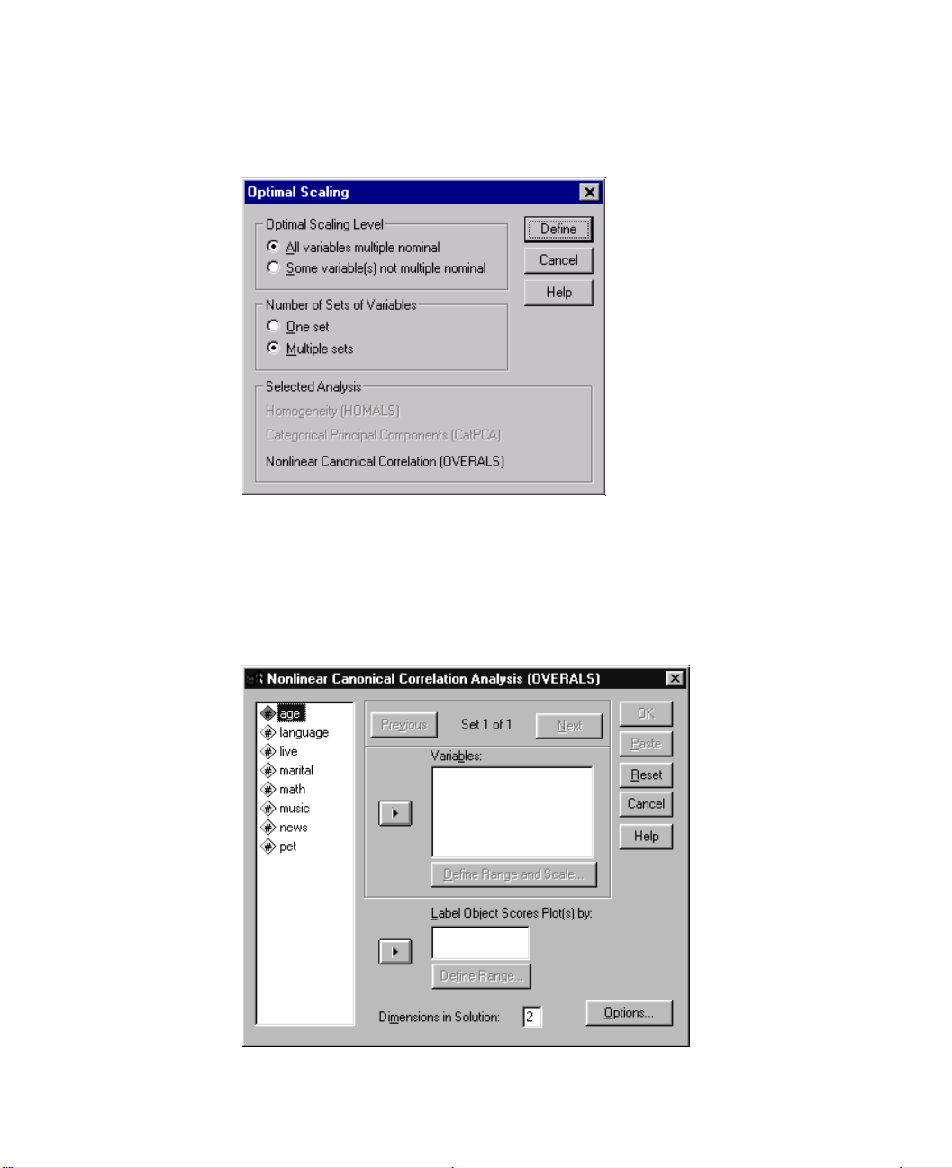
Nonlinear Canonical Correlation Analysis (OVERALS) 43
Figure 4.1 Optimal Scaling dialog box
Select Multiple sets.
Select either Some variable(s) not multiple nominal or All variables multiple nominal.
Click Define.
Figure 4.2 Nonlinear Canonical Correlation Analysis (OVERALS) dialog box
Page 56

44 Chapter 4
Define at least two sets of variables. Select the variable(s) that you want to include in
Define the value range and measurement scale (optimal scaling level) for each selected
Click OK.
the first set. To move to the next set, click
to include in the second set. You can add additional sets as desired. Click
Next, and select the variables that you want
Previous to
return to the previously defined variable set.
variable.
Optionally, you can:
• Select one or more variables to provide point labels for object scores plots. Each variable produces a separate plot, with the points labeled by the values of that variable.
You must define a range for each of these plot label variables. Using the dialog box,
a single variable cannot be used both in the analysis and as a labeling variable. If labeling the object scores plot with a variable used in the analysis is desired, use the
Compute
facility on the Transform menu to create a copy of that variable. Use the
new variable to label the plot. Alternatively, command syntax can be used.
• Specify the number of dimensions you want in the solution. In general, choose as few
dimensions as needed to explain most of the variation. If the analysis involves more
than two dimensions, SPSS produces three-dimensional plots of the first three dimensions. Other dimensions can be displayed by editing the chart.
Define Range and Scale in OVERALS
You must define a range for each variable. The maximum value specified must be an
integer. Fractional data values are truncated in the analysis. A category value that is
outside of the specified range is ignored in the analysis. To minimize output, use the
Automatic Recode facility on the Transform menu to create consecutive categories
beginning with 1 for variables treated as nominal or ordinal. Recoding to consecutive
integers is not recommended for variables scaled at the numerical level. To minimize
output for variables treated as numerical, for each variable, subtract the minimum
value from every value and add 1.
You must also select the scaling to be used to quantify each variable.
Ordinal. The order of the categories of the observed variable is preserved in the quantified variable.
Single nominal. Objects in the same category receive the same score. When all variables
are single nominal, the first dimension of this solution is the same as that of the first homogeneity analysis dimension.
Page 57
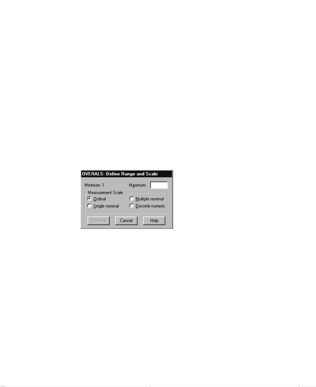
Nonlinear Canonical Correlation Analysis (OVERALS) 45
Multiple nominal. The quantifications can be different for each dimension. When all
variables are multiple nominal and there is only one variable in each set, categorical canonical correlation analysis with optimal scaling produces the same results as homogeneity analysis.
Discrete numeric. Categories are treated as ordered and equally spaced. The differences
between category numbers and the order of the categories of the observed variable are
preserved in the quantified variable. When all variables are at the numerical level and
there are two sets, the analysis is analogous to classical canonical correlation analysis.
To De fine an Optimal Scaling Range and Scale in OVERALS
In the OVERALS dialog box, select one or more variables in the Variables list.
Click Define Range and Scale.
Figure 4.3 OVERALS Define Range and Scale dialog box
Enter the maximum value for the variable. A minimum value of 1 is displayed. This
minimum value cannot be changed.
Select the measurement (optimal scaling) scale to be used in the analysis.
Click Continue.
Define Range in OVERALS
You must define a range for each variable used to label the object scores plots. The
maximum value specified must be an integer. Fractional data values are truncated in
the analysis. Labels for category values outside of the specified range for a labeling
variable do not appear in the plots. All cases with such category values are labeled with
a single label corresponding to a data value outside of the defined range.
Page 58
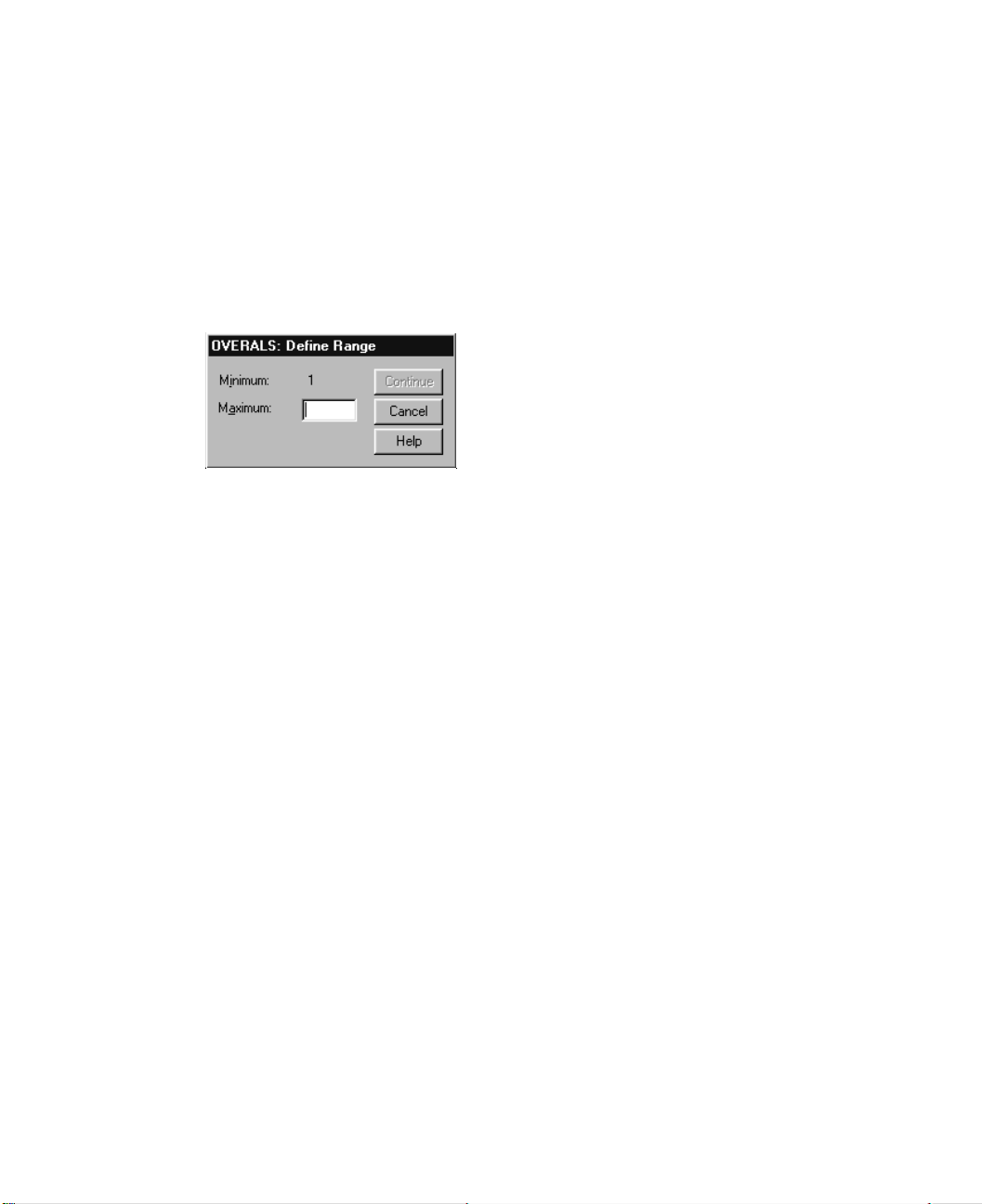
46 Chapter 4
To Define an Optimal Scaling Range in OVERALS
Select a variable for Label Object Scores Plot(s) By in the Nonlinear Canonical Corre-
lation Analysis (OVERALS) dialog box.
Click Define Range.
Figure 4.4 OVERALS Define Range dialog box
Enter the maximum value for the variable. A minimum value of 1 is displayed. This
minimum value cannot be changed.
Click Continue.
Nonlinear Canonical Correlation Analys is Options
The Options dialog box allows you to select optional statistics and plots, save object
scores as new variables in the working data file, specify iteration and convergence criteria, and specify an initial configuration for the analysis.
Page 59
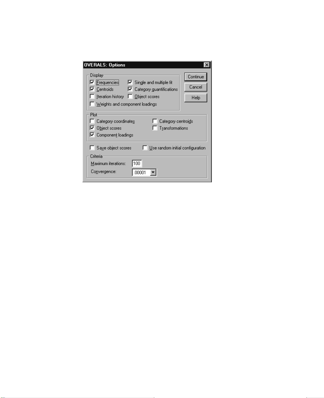
Nonlinear Canonical Correlation Analysis (OVERALS) 47
Figure 4.5 OVERALS Options dialog box
Display. Available statistics include marginal frequencies (counts), centroids, iteration
history, weights and component loadings, category quantifications, object scores, and
single and multiple fit statistics.
Plot. You can produce plots of category coordinates, object scores, component loadings,
category centroids, and transformations.
Save object scores. You can save the object scores as new variables in the working data
file. Object scores are saved for the number of dimensions specified in the main dialog
box.
Use random initial configuration. A random initial configuration should be used if all or
some of the variables are single nominal. If this option is not selected, a nested initial
configuration is used.
Criteria. You can specify the maximum number of iterations the nonlinear canonical correlation analysis can go through in its computations. You can also select a convergence
criterion value. The analysis stops iterating if the difference in total fit between the last
two iterations is less than the convergence value or if the maximum number of iterations
is reached.
Page 60

48 Chapter 4
OVERALS Command Additional Features
You can customize your nonlinear canonical correlation analysis if you paste your selections into a syntax window and edit the resulting
command language also allows you to:
• Specify the dimension pairs to be plotted, rather than plotting all extracted dimensions (using the
• Specify the number of value label characters used to label points on the plots (with
PLOT subcommand).
the
• Designate more than five variables as labeling variables for object scores plots (with
the
PLOT subcommand).
• Select variables used in the analysis as labeling variables for the object scores plots
(with the
• Select variables to provide point labels for the quantification score plot (with the
PLOT subcommand).
• Specify the number of cases to be included in the analysis, if you do not want to use
all cases in the working data file (with the
• Specify rootnames for variables created by saving object scores (with the
subcommand).
• Specify the number of dimensions to be saved, rather than saving all extracted dimensions (with the
• Write category quantifications to a matrix file (using the
• Produce low-resolution plots that may be easier to read than the usual high-resolution
plots (using the
• Produce centroid and transformation plots for specified variables only (with the
PLOT subcommand).
NDIM keyword on the PLOT subcommand).
PLOT subcommand).
SAVE subcommand).
SET command).
OVERALS command syntax. SPSS
NOBSERVATIONS subcommand).
SAVE
MATRIX subcommand).
Page 61

5
Correspondence Analysis
One of the goals of correspondence analysis is to describe the relationships between
two nominal variables in a correspondence table in a low-dimensional space, while simultaneously describing the relationships between the categories for each variable. For
each variable, the distances between category points in a plot reflect the relationships
between the categories with similar categories plotted close to each other. Projecting
points for one variable on the vector from the origin to a category point for the other
variable describe the relationship between the variables.
An analysis of contingency tables often includes examining row and column profiles and testing for independence via the chi-square statistic. However, the number of
profiles can be quite large, and the chi-square test does not reveal the dependence structure. The Crosstabs procedure offers several measures of association and tests of
association but cannot graphically represent any relationships between the variables.
Factor analysis is a standard technique for describing relationships between variables in a low-dimensional space. However, factor analysis requires interval data, and
the number of observations should be five times the number of variables. Correspondence analysis, on the other hand, assumes nominal variables and can describe the
relationships between categories of each variable, as well as the relationship between
the variables. In addition, correspondence analysis can be used to analyze any table of
positive correspondence measures.
Example. Correspondence analysis could be used to graphically display the relation-
ship between staff category and smoking habits. You might find that with regard to
smoking, junior managers differ from secretaries, but secretaries do not differ from senior managers. You might also find that heavy smoking is associated with junior managers, whereas light smoking is associated with secretaries.
Statistics and plots. Correspondence measures, row and column profiles, singular val-
ues, row and column scores, inertia, mass, row and column score confidence statistics,
singular value confidence statistics, transformation plots, row point plots, column point
plots, and biplots.
Data. Categorical variables to be analyzed are scaled nominally. For aggregated data or
for a correspondence measure other than frequencies, use a weighting variable with
positive similarity values. Alternatively, for table data, use syntax to read the table.
49
Page 62
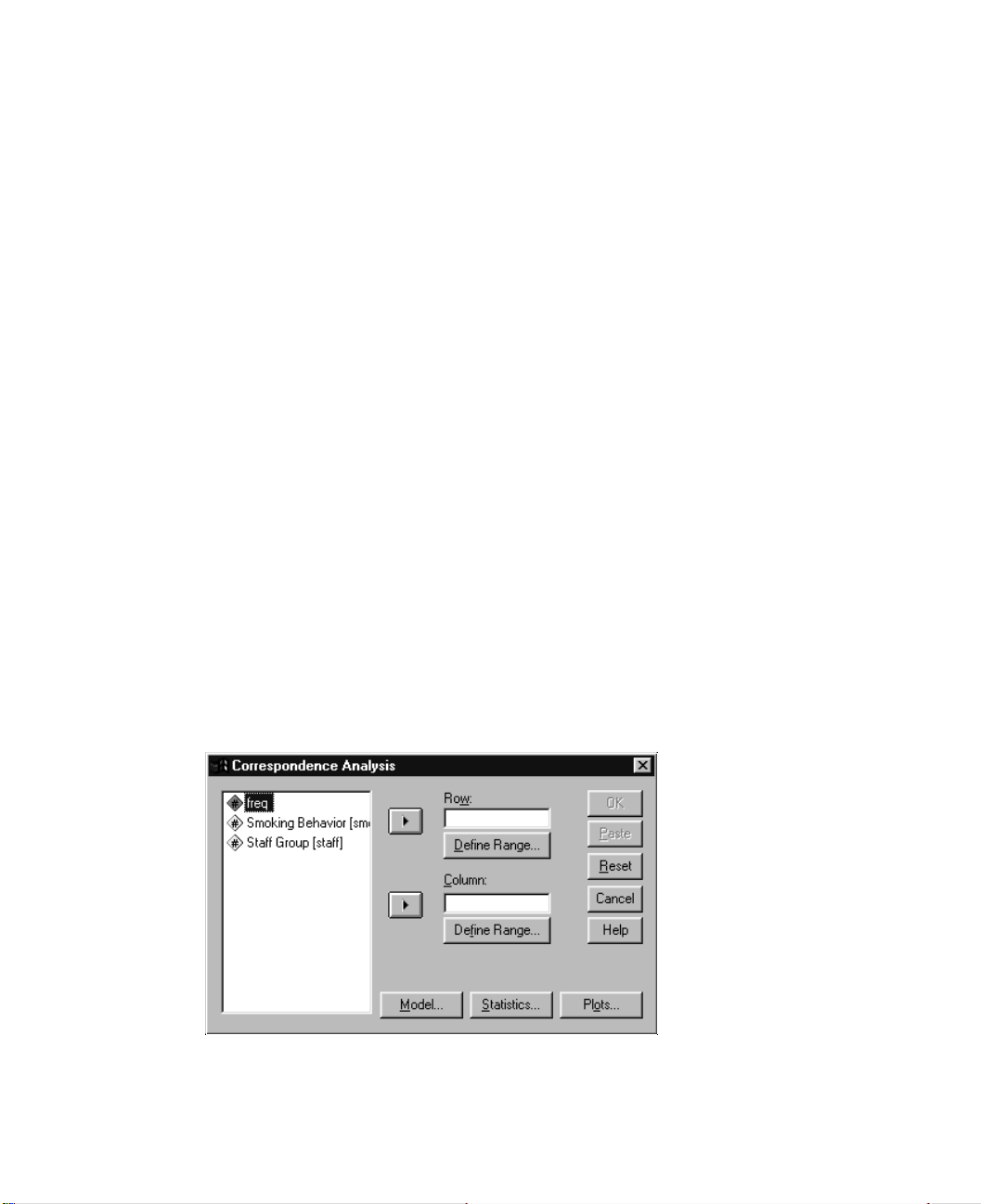
50 Chapter 5
Assumptions. The maximum number of dimensions used in the procedure depends on
the number of active rows and column categories and the number of equality constraints.
If no equality constraints are used and all categories are active, the maximum dimensionality is one fewer than the number of categories for the variable with the fewest categories. For example, if one variable has five categories and the other has four, the
maximum number of dimensions is three. Supplementary categories are not active. For
example, if one variable has five categories, two of which are supplementary, and the
other variable has four categories, the maximum number of dimensions is two. Treat all
sets of categories that are constrained to be equal as one category. For example, if a variable has five categories, three of which are constrained to be equal, that variable should
be treated as having three categories when determining the maximum dimensionality.
Two of the categories are unconstrained, and the third category corresponds to the three
constrained categories. If you specify a number of dimensions greater than the maximum, the maximum value is used.
Related procedures. If more than two variables are involved, use homogeneity analysis.
If the variables should be scaled ordinally, use principal components analysis with optimal scaling.
To Obtain a Correspondence Analysis
From the menus choose:
Analyze
Data Reduction
Correspondence Analysis…
Figure 5.1 Correspondence Analysis dialog box
Page 63

Select a row variable.
Select a column variable.
Define the ranges for the variables.
Click OK.
Define Row Range in Correspondence Analysis
You must define a range for the row variable. The minimum and maximum values specified must be integers. Fractional data values are truncated in the analysis. A category
value that is outside of the specified range is ignored in the analysis.
All categories are initially unconstrained and active. You can constrain row catego-
ries to equal other row categories, or you can define a row category as supplementary.
• Categories must be equal. Categories must have equal scores. Use equality con-
straints if the obtained order for the categories is undesirable or counterintuitive. The
maximum number of row categories that can be constrained to be equal is the total
number of active row categories minus 1. To impose different equality constraints on
sets of categories, use syntax. For example, use syntax to constrain categories 1 and
2 to be equal and categories 3 and 4 to be equal.
• Category is supplemental. Supplementary categories do not influence the analysis
but are represented in the space defined by the active categories. Supplementary categories play no role in defining the dimensions. The maximum number of supplementary row categories is the total number of row categories minus 2.
Correspondence Analysis 51
To Define a Row Range in Correspondence Analys is
Select the row variable in the Correspondence Analysis dialog box.
Click Define Range.
Page 64
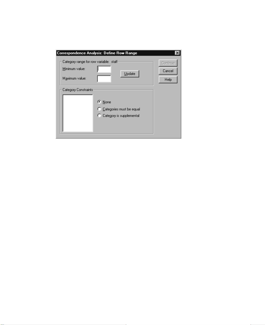
52 Chapter 5
Click Update.
Figure 5.2 Correspondence Analysis Define Row Range dialog box
Enter the minimum and maximum values for the row variable.
Click Continue.
Optionally, you can specify equality constraints on the row variable categories and define categories to be supplementary. For each category to be constrained or supplementary, select the category from the list of categories generated by
Category is supplemental or Categories must be equal. For equality constraints, at least
two categories must be designated as equal.
Define Column Range in Correspondence Analysis
You must define a range for the column variable. The minimum and maximum values
specified must be integers. Fractional data values are truncated in the analysis. A category value that is outside of the specified range is ignored in the analysis.
All categories are initially unconstrained and active. You can constrain column categories to equal other column categories or you can define a column category as
supplementary.
• Categories must be equal. Categories must have equal scores. Use equality con-
straints if the obtained order for the categories is undesirable or counterintuitive. The
maximum number of column categories that can be constrained to be equal is the to-
tal number of active column categories minus 1. To impose different equality con-
Update and choose
Page 65
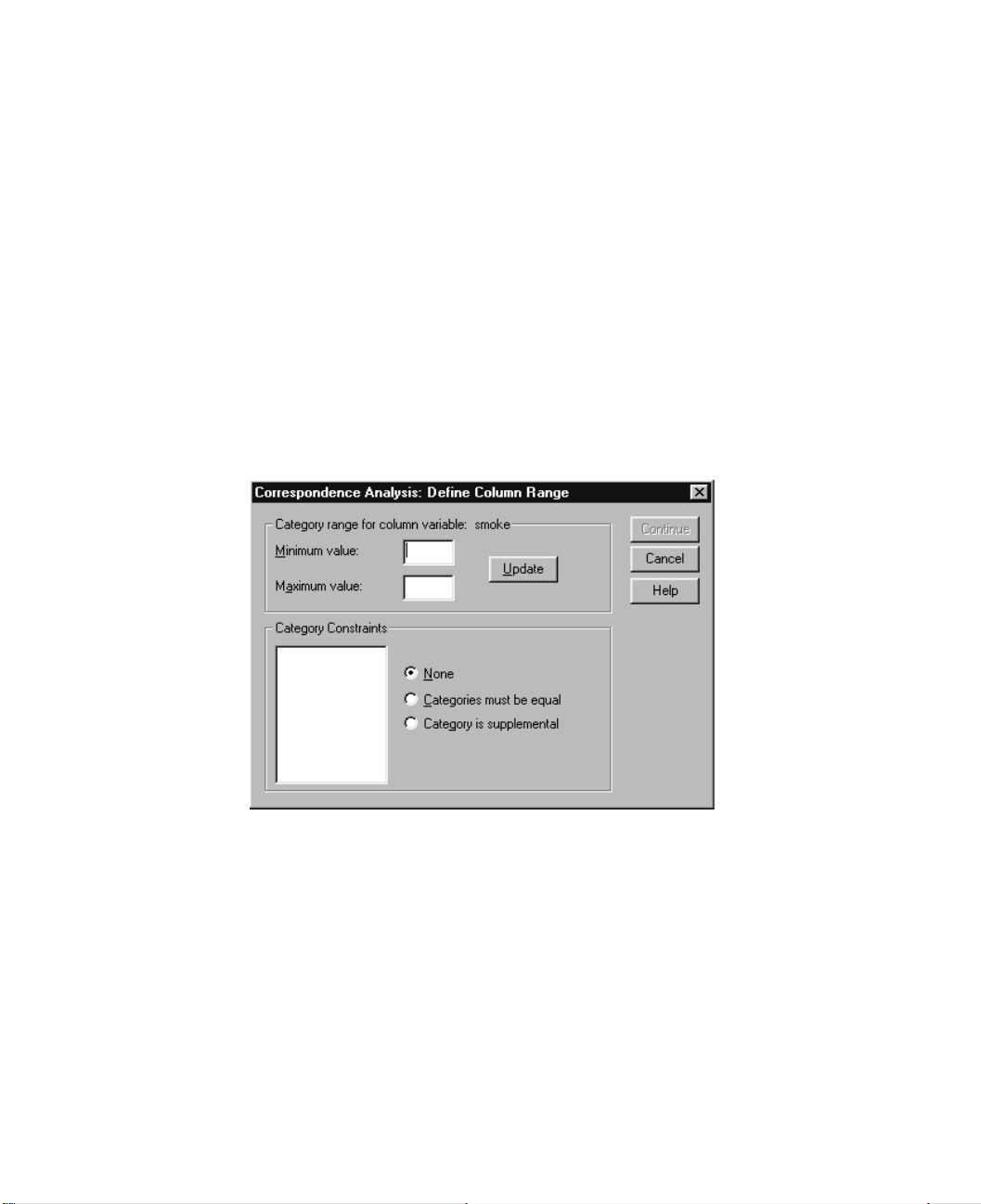
straints on sets of categories, use syntax. For example, use syntax to constrain
categories 1 and 2 to be equal and categories 3 and 4 to be equal.
• Category is supplemental. Supplementary categories do not influence the analysis
but are represented in the space defined by the active categories. Supplementary categories play no role in defining the dimensions. The maximum number of supplementary column categories is the total number of column categories minus 2.
To Define a Column Range in Corre spondence Analysis
Select the column variable in the Correspondence Analysis dialog box.
Click Define Range.
Figure 5.3 Correspondence Analysis Define Column Range dialog box
Correspondence Analysis 53
Enter the minimum and maximum values for the column variable.
Click Update.
Click Continue.
Optionally, you can specify equality constraints on the column variable categories and
define categories to be supplementary. For each category to be constrained or supplementary, select the category from the list of categories generated by
Category is supplemental or Categories must be equal. For equality constraints, at least
Update and choose
two categories must be designated as equal.
Page 66
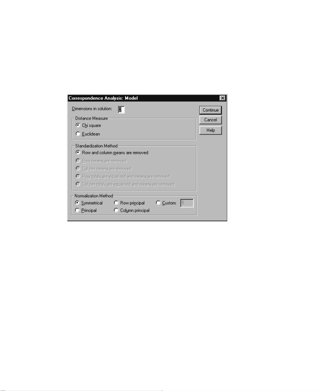
54 Chapter 5
Correspondence Analysis Model
The Model dialog box allows you to specify the number of dimensions, the distance
measure, the standardization method, and the normalization method.
Figure 5.4 Correspondence Analysis Model dialog box
Dimensions in solution. Specify the number of dimensions. In general, choose as few
dimensions as needed to explain most of the variation. The maximum number of dimensions depends on the number of active categories used in the analysis and on the equality
constraints. The maximum number of dimensions is the smaller of:
• The number of active row categories minus the number of row categories constrained
to be equal, plus the number of constrained row category sets
• The number of active column categories minus the number of column categories constrained to be equal, plus the number of constrained column category sets
Distance Measure. You can select the measure of distance among the rows and columns
of the correspondence table. Choose one of the following alternatives:
• Chi square. Use a weighted profile distance, where the weight is the mass of the rows
or columns. This measure is required for standard correspondence analysis.
• Euclidean. Use the square root of the sum of squared differences between pairs of
rows and pairs of columns.
Page 67

Correspondence Analysis 55
Standardization Method. Choose one of the following alternatives:
• Row and column means are removed. Both the rows and columns are centered. This
method is required for standard correspondence analysis.
• Row means are removed. Only the rows are centered.
• Column means are removed. Only the columns are centered.
• Row totals are equalized and means are removed. Before centering the rows, the row
margins are equalized.
• Column totals are equalized and means are removed. Before centering the columns,
the column margins are equalized.
Normalization Method. Choose one of the following alternatives:
• Symmetrical. For each dimension, the row scores are the weighted average of the col-
umn scores divided by the matching singular value, and the column scores are the
weighted average of row scores divided by the matching singular value. Use this
method if you want to examine the differences or similarities between the categories
of the two variables.
• Principal. The distances between row points and column points are approximations
of the distances in the correspondence table according to the selected distance measure. Use this method if you want to examine differences between categories of either
or both variables instead of differences between the two variables.
• Row principal. The distances between row points are approximations of the distances
in the correspondence table according to the selected distance measure. The row
scores are the weighted average of the column scores. Use this method if you want
to examine differences or similarities between categories of the row variable.
• Column principal. The distances between column points are approximations of the
distances in the correspondence table according to the selected distance measure. The
column scores are the weighted average of the row scores. Use this method if you
want to examine differences or similarities between categories of the column
variable.
• Custom. You must specify a value between –1 and 1. A value of –1 corresponds to
column principal. A value of 1 corresponds to row principal. A value of 0 corresponds to symmetrical. All other values spread the inertia over both the row and column scores to varying degrees. This method is useful for making tailor-made biplots.
Page 68
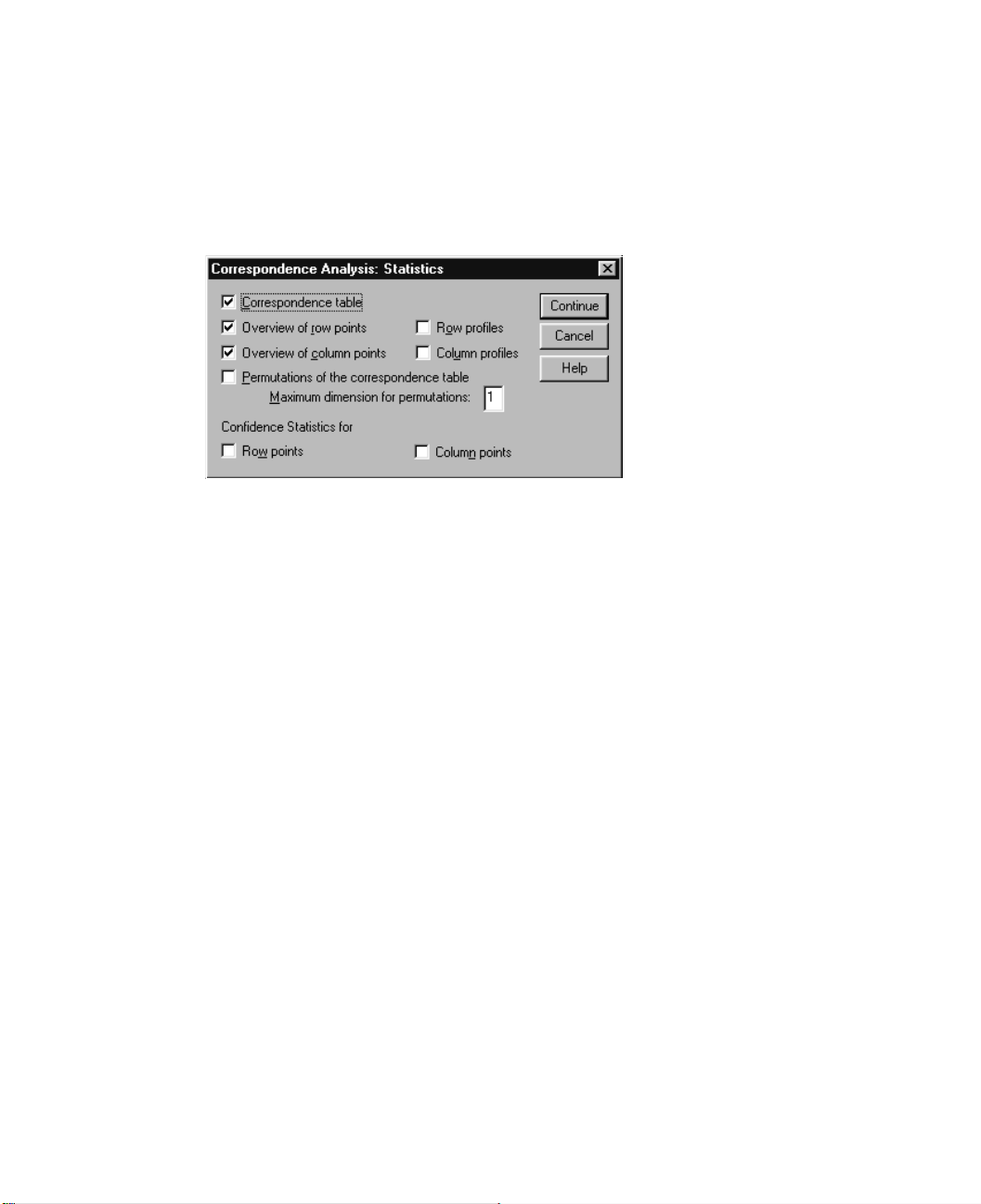
56 Chapter 5
Correspondence Analysis Statistics
The Statistics dialog box allows you to specify the numerical output produced.
Figure 5.5 Correspondence Analysis Statistics dialog box
Correspondence table. A crosstabulation of the input variables with row and column
marginal totals.
Overview of row points. For each row category, the scores, mass, inertia, contribution to
the inertia of the dimension, and the contribution of the dimension to the inertia of the
point.
Overview of column points. For each column category, the scores, mass, inertia, contribution to the inertia of the dimension, and the contribution of the dimension to the inertia
of the point.
Row profiles. For each row category, the distribution across the categories of the column
variable.
Column profiles. For each column category, the distribution across the categories of the
row variable.
Permutations of the correspondence table. The correspondence table reorganized such
that the rows and columns are in increasing order according to the scores on the first dimension. Optionally, you can specify the maximum dimension number for which permuted tables will be produced. A permuted table for each dimension from 1 to the
number specified is produced.
Confidence Statistics for Row points. Includes standard deviation and correlations for
all nonsupplementary row points.
Confidence Statistics for Column points. Includes standard deviation and correlations
for all nonsupplementary column points.
Page 69
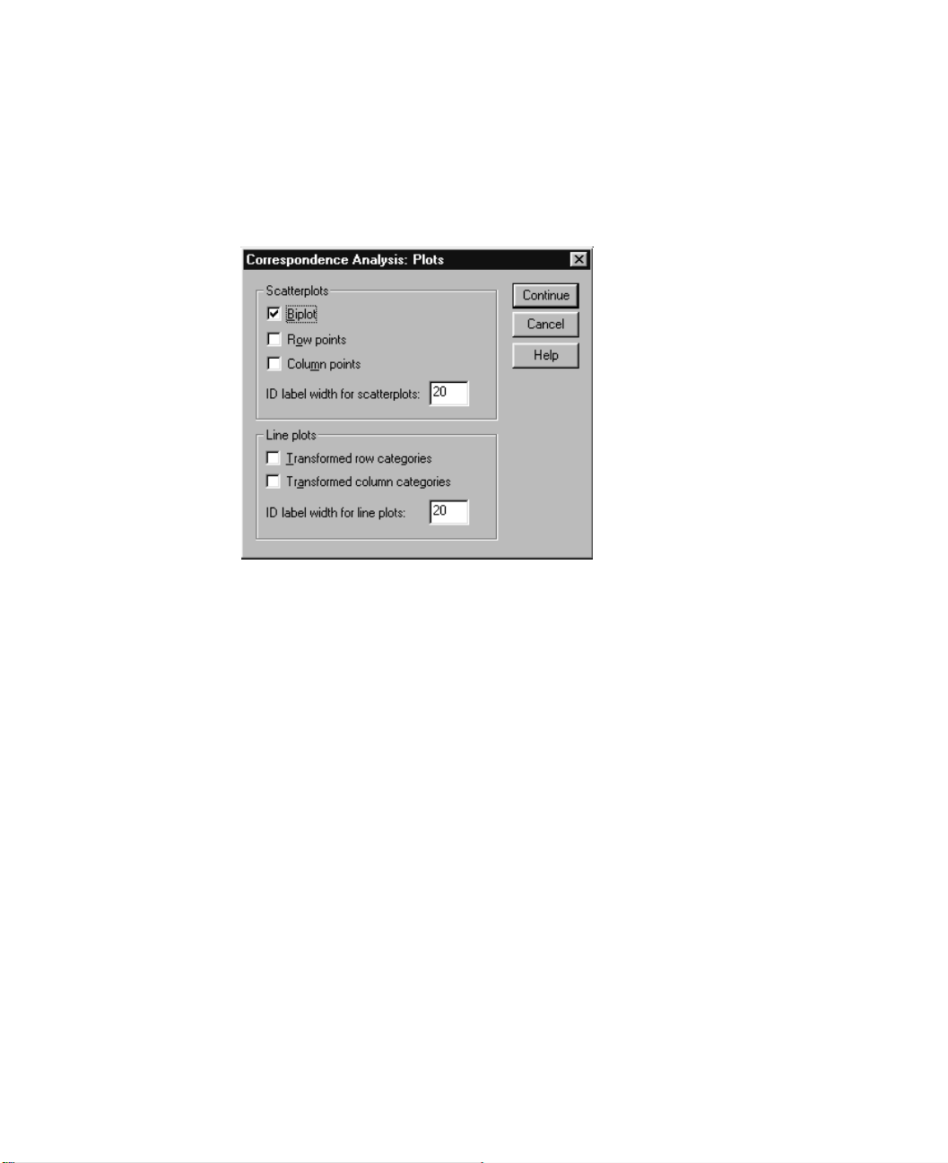
Correspondence Analysis Plots
The Plots dialog box allows you to specify which plots are produced.
Figure 5.6 Correspondence Analysis Plots dialog box
Scatterplots. Produces a matrix of all pairwise plots of the dimensions. Available scatterplots include:
• Biplot. Produces a matrix of joint plots of the row and column points. If principal nor-
malization is selected, the biplot is not available.
• Row points. Produces a matrix of plots of the row points.
• Column points. Produces a matrix of plots of the column points.
Correspondence Analysis 57
Optionally, you can specify how many value label characters to use when labeling the
points. This value must be a non-negative integer less than or equal to 20.
Line plots. Produces a plot for every dimension of the selected variable. Available line
plots include:
• Transformed row categories. Produces a plot of the original row category values
against their corresponding row scores.
• Transformed column categories. Produces a plot of the original column category val-
ues against their corresponding column scores.
Optionally, you can specify how many value label characters to use when labeling the
category axis. This value must be a non-negative integer less than or equal to 20.
Page 70

58 Chapter 5
CORRESPONDENCE Command Additional Features
You can customize your correspondence analysis if you paste your selections into a syntax window and edit the resulting
mand language also allows you to:
• Specify table data as input instead of using casewise data (using the
subcommand).
• Specify the number of value-label characters used to label points for each type of
scatterplot matrix or biplot matrix (with the
• Specify the number of value-label characters used to label points for each type of line
plot (with the
PLOT subcommand).
• Write a matrix of row and column scores to an SPSS matrix data file (with the
OUTFILE subcommand).
• Write a matrix of confidence statistics (variances and covariances) for the singular
values and the scores to an SPSS matrix data file (with the
• Specify multiple sets of categories to be equal (with the
CORRESPONDENCE command syntax. SPSS com-
TABLE = ALL
PLOT subcommand).
OUTFILE subcommand).
EQUAL subcommand).
Page 71

6
Homogeneity Analysis (HOMALS)
Homogeneity analysis quantifies nominal (categorical) data by assigning numerical
values to the cases (objects) and categories. Homogeneity analysis is also known by the
acronym HOMALS, for homogeneity analysis by means of alternating least squares.
The goal of HOMALS is to describe the relationships between two or more nominal
variables in a low-dimensional space containing the variable categories as well as the
objects in those categories. Objects within the same category are plotted close to each
other, whereas objects in different categories are plotted far apart. Each object is as
close as possible to the category points for categories that contain that object.
Homogeneity analysis is similar to correspondence analysis but is not limited to two
variables. As a result, homogeneity analysis is also known in the literature as multiple
correspondence analysis. Homogeneity analysis can also be viewed as a principal components analysis of nominal data.
Homogeneity analysis is preferred over standard principal components analysis
when linear relationships between the variables may not hold or when variables are
measured at a nominal level. Moreover, output interpretation is more straightforward
in HOMALS than in other categorical techniques, such as crosstabulation tables and
loglinear modeling. Because variable categories are quantified, techniques that require
numerical data can be applied to the quantifications in subsequent analyses.
Example. Homogeneity analysis could be used to graphically display the relationship
between job category, minority classification, and gender. You might find that minority
classification and gender discriminate between people, but that job category does not.
You might also find that the Latino and African-American categories are similar to
each other.
Statistics and plots. Frequencies, eigenvalues, iteration history, object scores, category
quantifications, discrimination measures, object scores plots, category quantifications
plots, discrimination measures plots.
Data. All variables are categorical (nominal optimal scaling level). Use integers to code
the categories. To minimize output, use consecutive integers beginning with 1 to code
each variable.
Assumptions. All variables in the analysis have category quantifications that can be
different for each dimension (multiple nominal). Only one set of variables will be used
in the analysis. The maximum number of dimensions used in the procedure is either the
59
Page 72
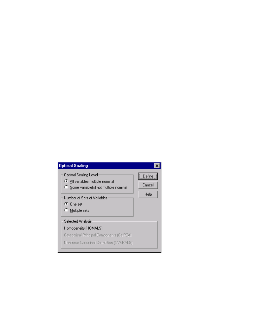
60 Chapter 6
total number of categories minus the number of variables with no missing data, or the
number of cases minus 1, whichever is smaller. For example, if one variable has five categories and the other has four (with no missing data), the maximum number of dimensions is seven ((5 + 4) – 2). If you specify a number greater than the maximum, the
maximum value is used.
Related procedures. For two variables, homogeneity analysis is analogous to correspondence analysis. If you believe that variables possess ordinal or numerical properties,
principal components with optimal scaling should be used. If you are interested in sets
of variables, nonlinear canonical correlation analysis should be used.
To Obtain a Homogeneity Analysis
From the menus choose:
Analyze
Data Reduction
Optimal Scaling...
Figure 6.1 Optimal Scaling dialog box
In the Optimal Scaling dialog box, select All variables multiple nominal.
Select One set.
Click Define.
Page 73
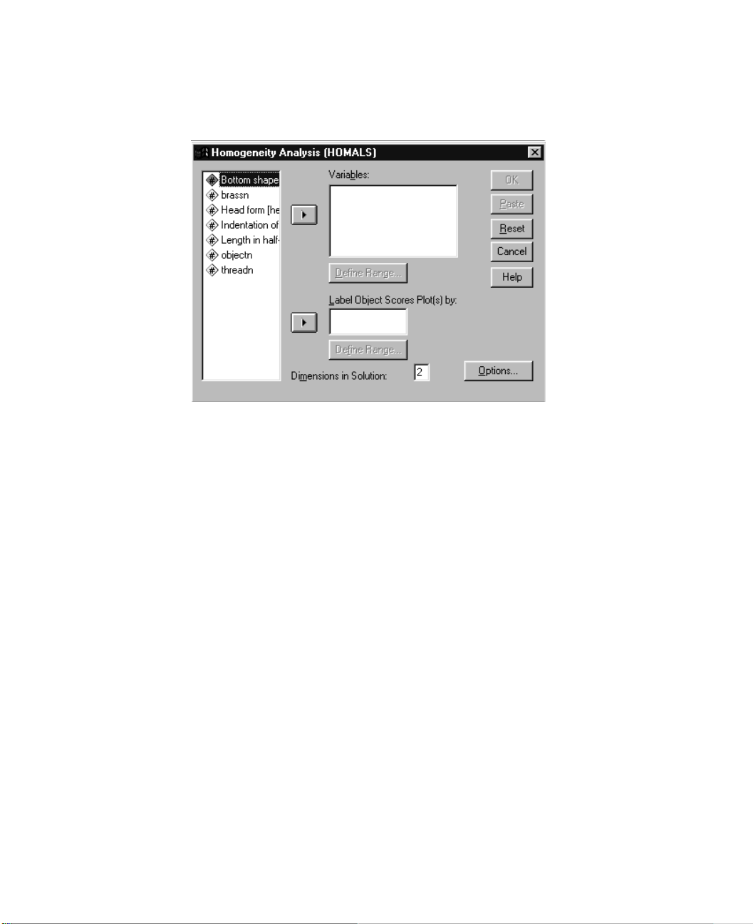
Figure 6.2 Homogeneity Analysis (HOMALS) dialog box
Select two or more variables.
Define the ranges for the variables.
Homogeneity Analysis (HOMALS) 61
Click OK.
Optionally, you can:
• Select one or more variables to provide point labels for object scores plots. Each vari-
able produces a separate plot, with the points labeled by the values of that variable.
You must define a range for each of these plot label variables. Using the dialog box,
a single variable cannot be used both in the analysis and as a labeling variable. If labeling the object scores plot with a variable used in the analysis is desired, use the
Compute
facility on the Transform menu to create a copy of that variable. Use the
new variable to label the plot. Alternatively, command syntax can be used.
• Specify the number of dimensions you want in the solution. In general, choose as few
dimensions as needed to explain most of the variation. If the analysis involves more
than two dimensions, SPSS produces three-dimensional plots of the first three dimensions. Other dimensions can be displayed by editing the chart.
Page 74
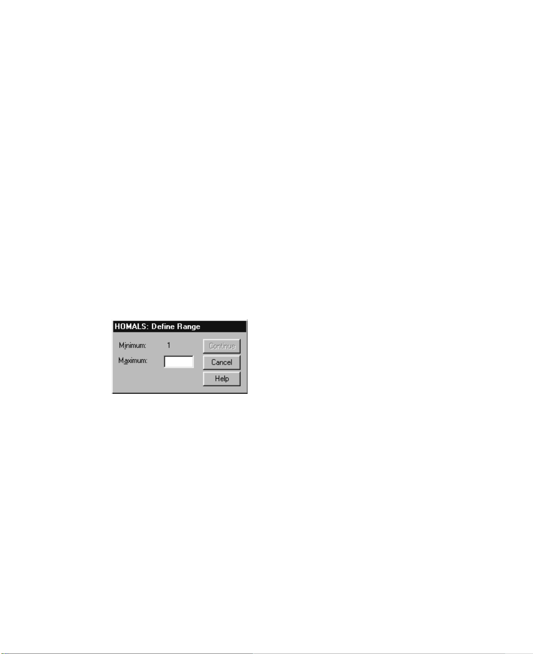
62 Chapter 6
Define Range in Homogeneity Analysis
You must define a range for each variable. The maximum value specified must be an
integer. Fractional data values are truncated in the analysis. A category value that is outside of the specified range is ignored in the analysis. To minimize output, use the Automatic Recode facility on the Transform menu to create consecutive categories beginning
with 1.
You must also define a range for each variable used to label the object scores plots.
However, labels for categories with data values outside of the defined range for the variable do appear on the plots.
To Define an Optimal Scaling Range in Homogeneity Analysis
Select one or more variables in the Variables list in the Homogeneity Analysis
(HOMALS) dialog box.
Click Define Range.
Figure 6.3 HOMALS Define Range dialog box
Enter the maximum value for the variable. A minimum value of 1 is displayed. This
minimum value cannot be changed.
Click Continue.
Page 75
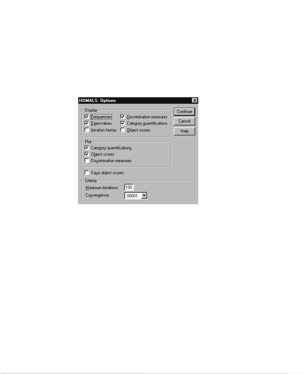
Homogeneity Analysis Options
The Options dialog box allows you to select optional statistics and plots, save object
scores as new variables in the working data file, and specify iteration and convergence
criteria.
Figure 6.4 HOMALS Options dialog box
Homogeneity Analysis (HOMALS) 63
Display. These options control what statistics are included in the output. Available statistics include marginal frequencies, eigenvalues, iteration history, discrimination measures, category quantifications, and object scores.
Plot. These options produce plots of category quantifications, object scores, and discrimination measures.
Save object scores. You can save the object scores as new variables in the working data
file. Object scores are saved for the number of dimensions specified in the main dialog
box.
Criteria. You can specify the maximum number of iterations the homogeneity analysis
can go through in its computations. You can also select a convergence criterion value.
The homogeneity analysis stops iterating if the difference in total fit between the last two
iterations is less than the convergence value, or if the maximum number of iterations is
reached.
Page 76

64 Chapter 6
HOMALS Command Additional Features
You can customize your homogeneity analysis if you paste your selections into a syntax
window and edit the resulting
also allows you to:
• Specify the dimension pairs to be plotted, rather than plotting all extracted dimensions (using the
NDIM keyword on the PLOT subcommand).
• Specify the number of value label characters used to label points on the plots (with
PLOT subcommand).
the
• Designate more than five variables as labeling variables for object scores plots (with
the
PLOT subcommand).
• Select variables used in the analysis as labeling variables for the object scores plots
(with the
PLOT subcommand).
• Select variables to provide point labels for the quantification score plot (with the
PLOT subcommand).
• Specify the number of cases to be included in the analysis if you do not want to use
all cases in the working data file (with the
• Specify rootnames for variables created by saving object scores (with the
subcommand).
• Specify the number of dimensions to be saved, rather than saving all extracted dimensions (with the
SAVE subcommand).
• Write category quantifications to a matrix file (using the
• Produce low-resolution plots that may be easier to read than the usual high-resolution
plots (using the
SET command).
HOMALS command syntax. SPSS command language
NOBSERVATIONS subcommand).
SAVE
MATRIX subcommand).
Page 77

7
Multidimensional Scaling (PROXSCAL)
Multidimensional scaling attempts to find the structure in a set of proximity measures
between objects. This is accomplished by assigning observations to specific locations
in a conceptual low-dimensional space such that the distances between points in the
space match the given (dis)similarities as closely as possible. The result is a leastsquares representation of the objects in that low-dimensional space, which, in many
cases, will help you to further understand your data.
Example. Multidimensional scaling can be very useful in determining perceptual relationships. For example, when considering your product image, you can conduct a survey in order to obtain a data set that describes the perceived similarity (or proximity)
of your product to those of your competitors. Using these proximities and independent
variables (such as price), you can try to determine which variables are important to how
people view these products, and adjust your image accordingly.
Statistics and plots. Iteration history, Stress measures, Stress decomposition, coordinates of the common space, object distances within the final configuration, individual
space weights, individual spaces, transformed proximities, transformed independent
variables, Stress plots, common space scatterplots, individual space weight scatterplots, individual spaces scatterplots, transformation plots, Shepard residual plots, and
independent variables transformation plots.
Data. Data can be supplied in the form of proximity matrices or variables that are converted into proximity matrices. The matrices may be formatted in columns or across
columns. The proximities may be treated on the ratio, interval, ordinal, or spline scaling
levels.
Assumptions. At least three variables must be specified. The number of dimensions
may not exceed the number of objects minus one. Dimensionality reduction is omitted
if combined with multiple random starts. If only one source is specified, all models are
equivalent to the identity model; therefore, the analysis defaults to the identity model.
Related procedures. Scaling all variables at the numerical level corresponds to standard multidimensional scaling analysis.
65
Page 78
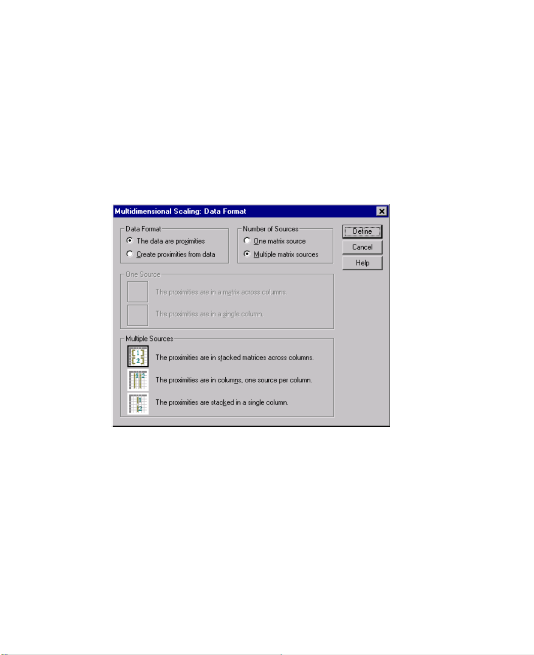
66 Chapter 7
To Obtain a Multidimensional Scaling
From the menus choose:
Analyze
Scale
Multidimensional Scaling (PROXSCAL)...
This opens the Data Format dialog box.
Figure 7.1 Multidimensional Scaling Data Format dialog box
You must specify the format of your data:
Data Format. Specify whether your data consist of proximity measures or you want to
create proximities from the data.
Number of Sources. If your data are proximities, specify whether you have a single
source or multiple sources of proximity measures.
One Source. If there is one source of proximities, specify whether your data set is formatted with the proximities in a matrix across the columns or in a single column with
two separate variables to identify the row and column of each proximity.
Multiple Sources. If there are multiple sources of proximities, specify whether the data
set is formatted with the proximities in stacked matrices across columns, in multiple columns with one source per column, or in a single column.
Page 79
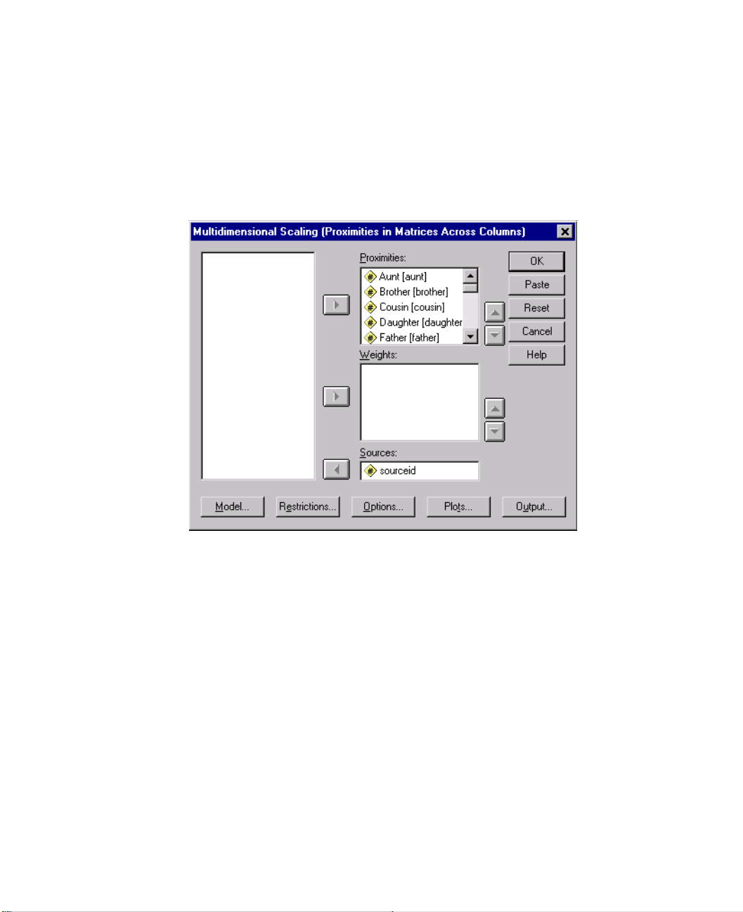
Proximities in Matrices across Columns
If you select the proximities in matrices data model for either one source or multiple
sources in the Data Format dialog box, the main dialog box will appear as follows:
Figure 7.2 Proximities in Matrices across Columns dialog box
Multidimensional Scaling (PROXSCAL) 67
Select three or more proximities variables. Please be sure that the order of the variables
in the list matches the order of the columns of the proximities.
Optionally, select a number of weights variables equal to the number of proximities
variables. Again, be sure that the order of the weights matches the order of the proximities they weight.
If there are multiple sources, optionally, select a sources variable. The number of cases
in each proximities variable should equal the number of proximities variables times the
number of sources.
Additionally, you can define a model for the multidimensional scaling, place restrictions
on the common space, set convergence criteria, specify the initial configuration to be
used, and choose plots and output.
Page 80
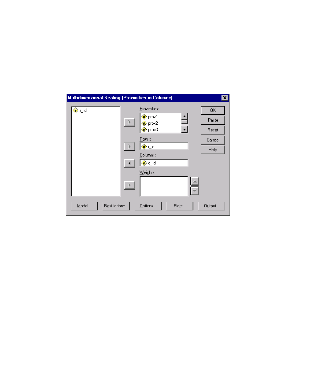
68 Chapter 7
Proximities in Columns
If you select the multiple columns model for multiple sources in the Data Format dialog
box, the main dialog box will appear as follows:
Figure 7.3 Proximities in Columns dialog box
Select two or more proximities variables. Each variable is assumed to be a matrix of
proximities from a separate source.
Select a rows variable. This defines the row locations for the proximities in each prox-
imities variable.
Select a columns variable. This defines the column locations for the proximities in each
proximities variable. Cells of the proximity matrix that are not given a row/column designation are treated as missing.
Optionally, select a number of weights variables equal to the number of proximities
variables.
Additionally, you can define a model for the multidimensional scaling, place restrictions
on the common space, set convergence criteria, specify the initial configuration to be
used, and choose plots and output.
Page 81
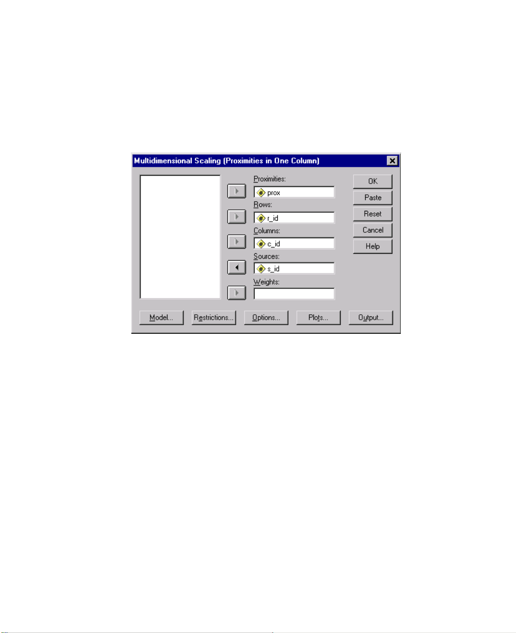
Proximities in One Column
If you select the one column model for either one source or multiple sources in the Data
Format dialog box, the main dialog box will appear as follows:
Figure 7.4 Proximities in One Column dialog box
Multidimensional Scaling (PROXSCAL) 69
Select a proximities variable. It is assumed to be one or more matrices of proximities.
Select a rows variable. This defines the row locations for the proximities in the proxim-
ities variable.
Select a columns variable. This defines the column locations for the proximities in the
proximities variable.
If there are multiple sources, select a sources variable. For each source, cells of the prox-
imity matrix that are not given a row/column designation are treated as missing.
Optionally, select a weights variable.
Additionally, you can define a model for the multidimensional scaling, place restrictions
on the common space, set convergence criteria, specify the initial configuration to be
used, and choose plots and output.
Page 82
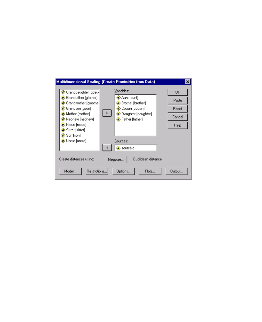
70 Chapter 7
Create Proximities from Data
If you choose to create proximities from the data in the Data Format dialog box, the main
dialog box will appear as follows:
Figure 7.5 Create Proximities from Data dialog box
If you create distances between variables (see the Measures dialog box), select at least
three variables. These will be used to create the proximity matrix (or matrices, if there
are multiple sources). If you create distances between cases, only one variable is needed.
If there are multiple sources, select a sources variable.
Optionally, choose a measure for creating proximities.
Additionally, you can define a model for the multidimensional scaling, place restrictions
on the common space, set convergence criteria, specify the initial configuration to be
used, and choose plots and output.
Page 83
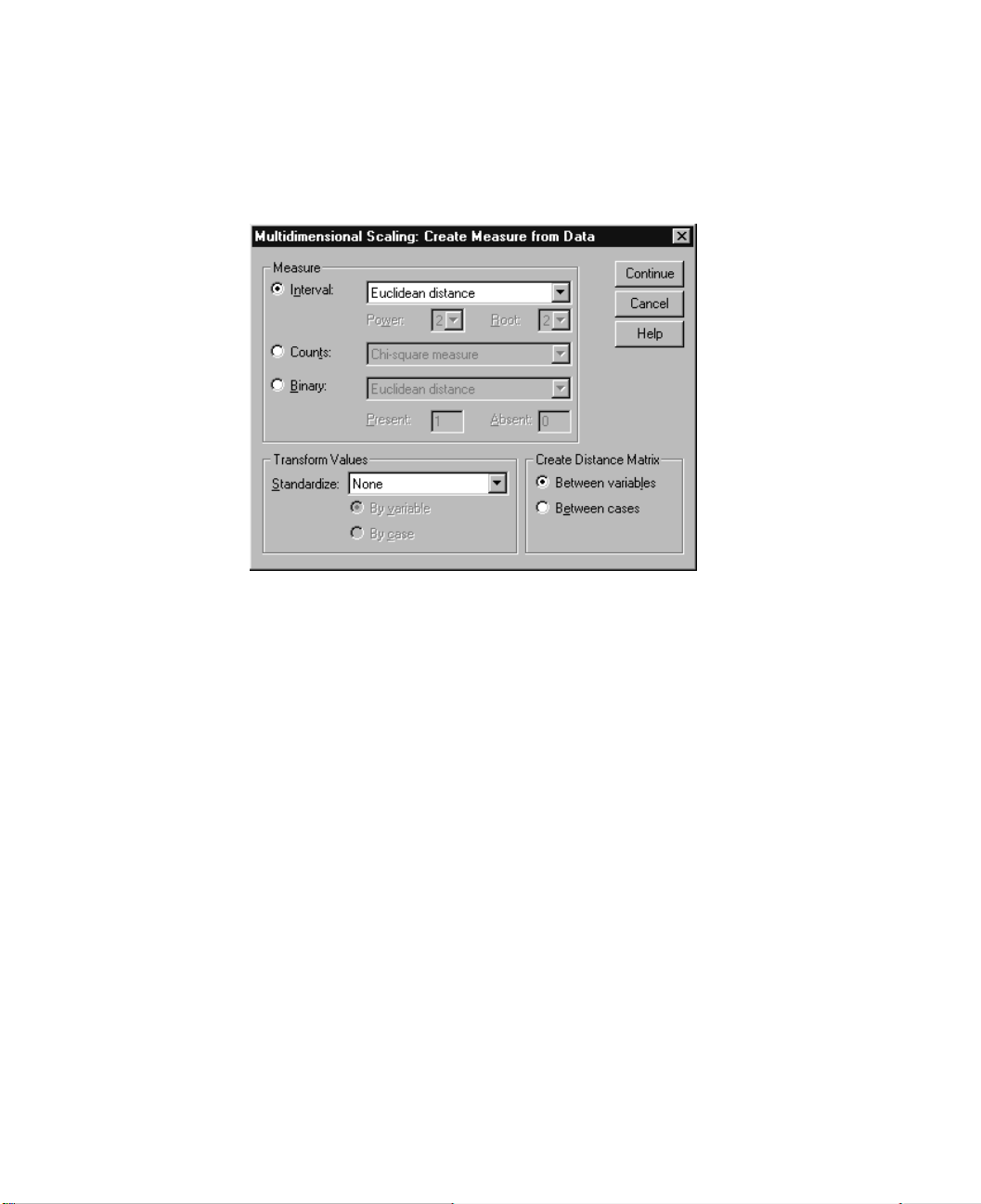
Measures Dialog Box
Figure 7.6 Multidimensional Scaling Create Measure from Data dialog box
Multidimensional Scaling (PROXSCAL) 71
Multidimensional scaling uses dissimilarity data to create a scaling solution. If your data
are multivariate data (values of measured variables), you must create dissimilarity data
in order to compute a multidimensional scaling solution. You can specify the details of
creating dissimilarity measures from your data.
Measure. Allows you to specify the dissimilarity measure for your analysis. Select one
alternative from the Measure group corresponding to your type of data, and then select
one of the measures from the drop-down list corresponding to that type of measure.
Available alternatives are:
• Interval. Euclidean distance, squared Euclidean distance, Chebychev, Block,
Minkowski, or Customized.
• Counts. Chi-square measure or Phi-square measure.
• Binary. Euclidean distance, Squared Euclidean distance, Size difference, Pattern dif-
ference, Variance, or Lance and Williams.
Create Distance Matrix. Allows you to choose the unit of analysis. Alternatives are Between variables or Between cases.
Transform Values. In certain cases, such as when variables are measured on very different scales, you may want to standardize values before computing proximities (not applicable to binary data). Select a standardization method from the Standardize drop-down
list (if no standardization is required, select
None).
Page 84
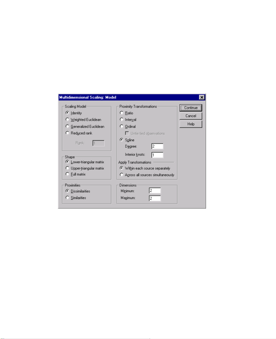
72 Chapter 7
Define a Multidimensional Scaling Model
The Model dialog box allows you to specify a scaling model, its minimum and maximum number of dimensions, the structure of the proximity matrix, the transformation to
use on the proximities, and whether proximities are transformed within each source separately, or unconditionally on the source.
Figure 7.7 Multidimensional Scal ing Model dialog box
Scaling Model. Choose from the following alternatives.
• Identity. All sources have the same configuration.
• Weighted Euclidean. This model is an individual differences model. Each source
has an individual space in which every dimension of the common space is weighted
differentially.
• Generalized Euclidean. This model is an individual differences model. Each source
has an individual space that is equal to a rotation of the common space, followed by
a differential weighting of the dimensions.
• Reduced rank. This is a Generalized Euclidean model for which you can specify the
rank of the individual space. You must specify a rank that is greater than or equal to
1 and less than the maximum number of dimensions.
Page 85

Multidimensional Scaling (PROXSCAL) 73
Shape. Specify whether the proximities should be taken from the lower-triangular part
or the upper-triangular part of the proximity matrix. You may specify that the full matrix
be used, in which case the weighted sum of the upper-triangular part and the lower-triangular part will be analyzed. In any case, the complete matrix should be specified, including the diagonal, though only the specified parts will be used.
Proximities. Specify whether your proximity matrix contains measures of similarity or
dissimilarity.
Proximity Transformations. Choose from the following alternatives.
• Ratio. The transformed proximities are proportional to the original proximities. This
is only allowed for positively valued proximities.
• Interval. The transformed proximities are proportional to the original proximities,
plus an intercept term. The intercept assures all transformed proximities to be
positive.
• Ordinal. The transformed proximities have the same order as the original proximities.
You may specify whether tied proximities should be kept tied or allowed to become
untied.
• Spline. The transformed proximities are a smooth nondecreasing piecewise polyno-
mial transformation of the original proximities. You may specify the degree of the
polynomial and the number of interior knots.
Apply Transformations. Specify whether only proximities within each source are compared with each other, or the comparisons are unconditional on the source.
Dimensions. By default, a solution is computed in two dimensions (Minimum=2, Maximum=2). You may choose an integer minimum and maximum from 1 to the number of
objects minus 1, so long as the minimum is less than or equal to the maximum. The procedure computes a solution in the maximum dimensions and then reduces the dimensionality in steps, until the lowest is reached.
Page 86
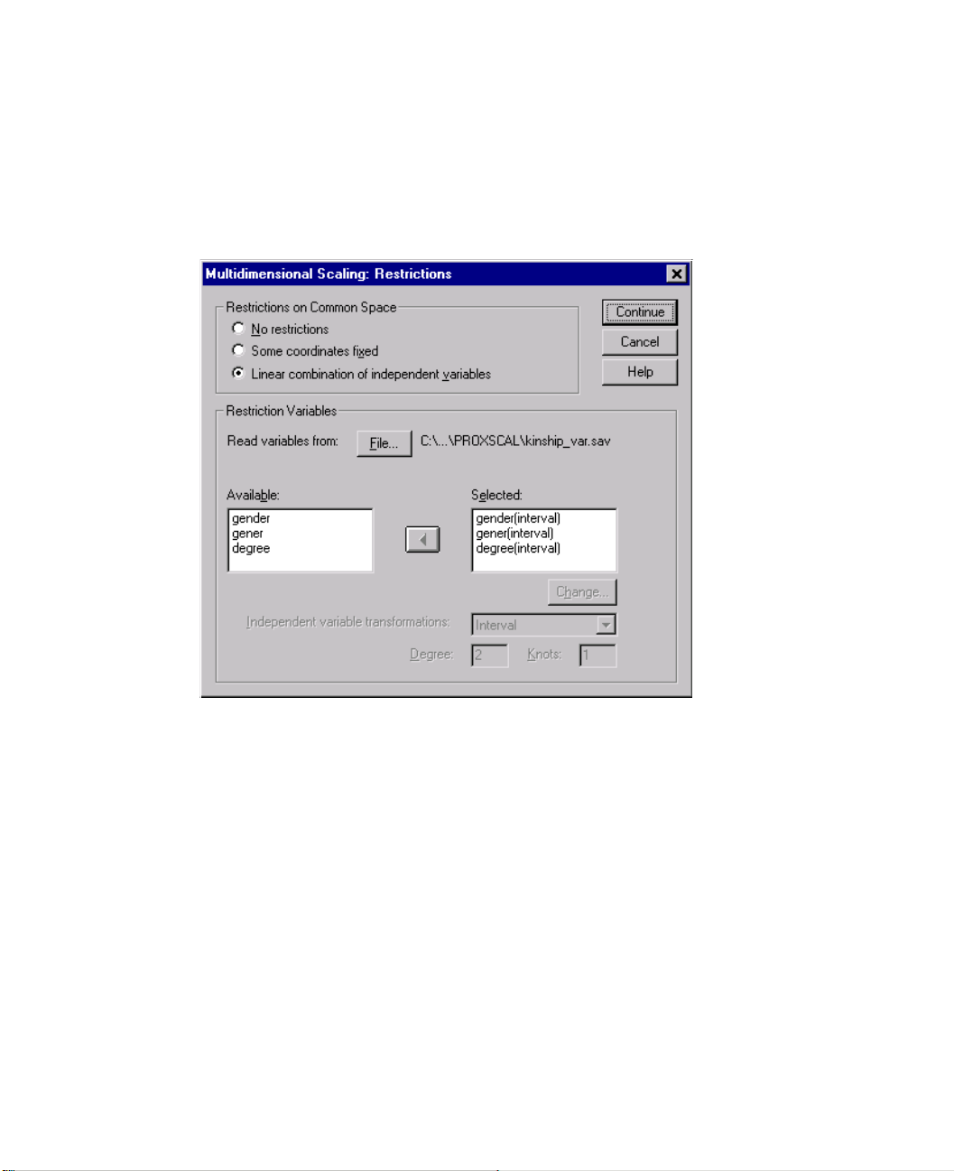
74 Chapter 7
Multidimensional Scaling Restrictions
The Restrictions dialog box allows you to place restrictions on the common space.
Figure 7.8 Multidimensional Scaling Restrictions dialog box
Restrictions on Common Space. Specify the type of restriction desired.
• No restrictions. No restrictions are placed on the common space.
• Some coordinates fixed. The first variable selected contains the coordinates of the
objects on the first dimension. The second variable corresponds to coordinates on the
second dimension, and so on. A missing value indicates that a coordinate on a dimension is free. The number of variables selected must equal the maximum number of
dimensions requested.
• Linear combination of independent variables. The common space is restricted to be
a linear combination of the variables selected.
Restriction Variables. Select the variables that define the restrictions on the common
space. If you specified a linear combination, you may specify an interval, nominal, ordinal, or spline transformation for the restriction variables. In either case, the number of
cases for each variable must equal the number of objects.
Page 87
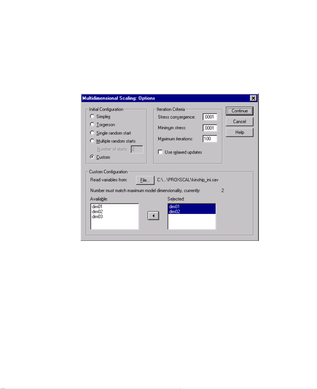
Multidimensional Scaling Options
The Options dialog box allows you to select the kind of initial configuration, specify iteration and convergence criteria, and select standard or relaxed updates.
Figure 7.9 Multidimensional Scaling Options dialog box
Multidimensional Scaling (PROXSCAL) 75
Initial Configuration. Choose one of the following alternatives.
• Simplex. Objects are placed at the same distance from each other in the maximum di-
mension. One iteration is taken to improve this high-dimensional configuration, followed by a dimensionality reduction operation to obtain an initial configuration that has
the maximum number of dimensions that you specified in the Model dialog box.
• Torgerson. A classical scaling solution is used as the initial configuration.
• Single random start. A configuration is chosen at random.
• Multiple random starts. Several configurations are chosen at random, and the solu-
tion with the lowest normalized raw Stress is shown.
• Custom. You may select variables that contain the coordinates of your own initial con-
figuration. The number of variables selected should equal the maximum number of
dimensions specified, with the first variable corresponding to coordinates on dimension 1, the second variable corresponding to coordinates on dimension 2, and so on.
The number of cases in each variable should equal the number of objects.
Page 88
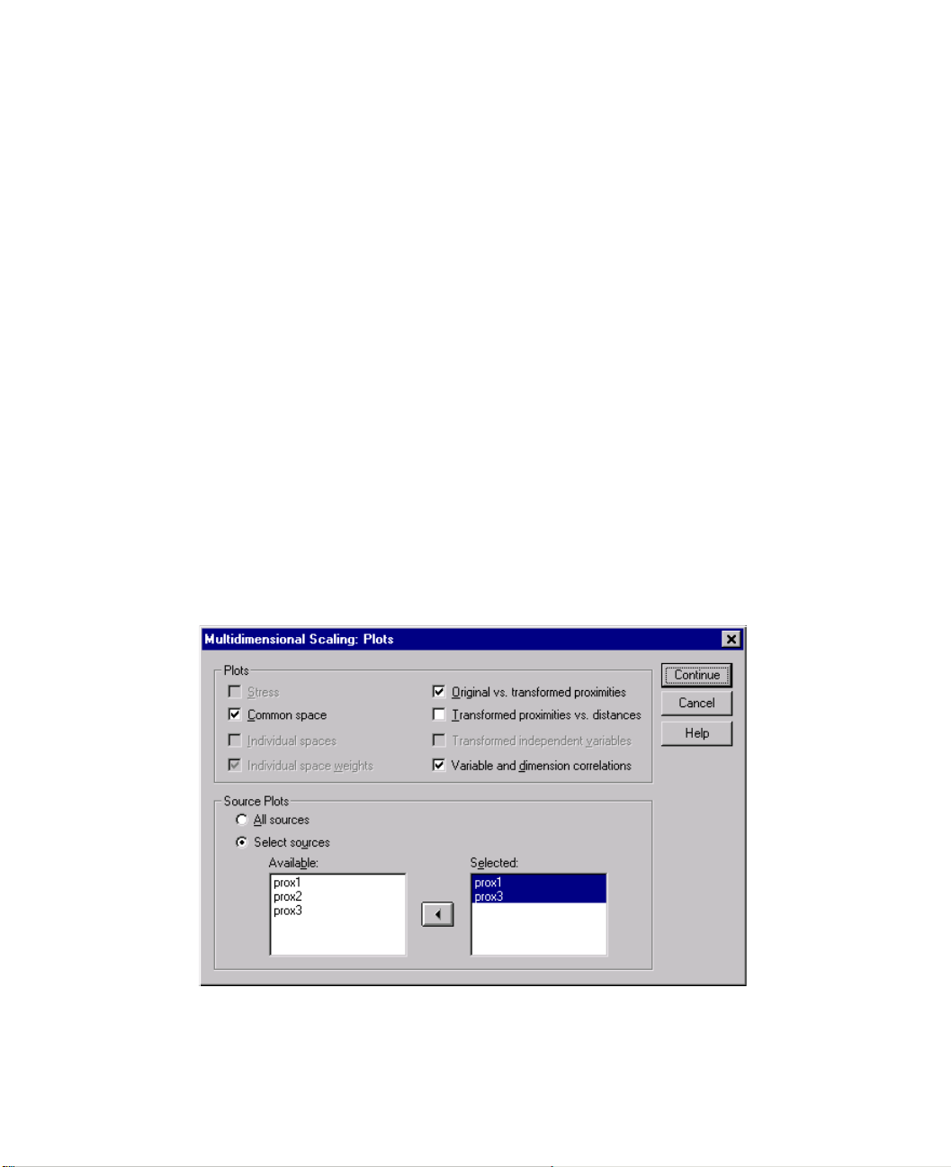
76 Chapter 7
Iteration Criteria. Specify the iteration criteria values.
• Stress convergence. The algorithm will stop iterating when the difference in consecutive normalized raw Stress values is less than the number specified here, which must
lie between 0.0 and 1.0.
• Minimum stress. The algorithm will stop when the normalized raw Stress falls below
the number specified here, which must lie between 0.0 and 1.0.
• Maximum iterations. The algorithm will perform the number of iterations specified
here, unless one of the above criteria is satisfied first.
• Use relaxed updates. Relaxed updates will speed up the algorithm; these cannot be
used with models other than the identity model, or with restrictions.
Multidimensional Scaling Plots, Version 1
The Plots dialog box allows you to specify which plots will be produced. If you have the
Proximities in Columns data format, the following Plots dialog box is displayed. For Individual space weights, Original vs. transformed proximities, and Transformed proximities vs. distances plots, you may specify the sources for which the plots should be
produced. The list of available sources is the list of proximities variables in the main dialog box.
Figure 7.10 Multidimensional Scaling Plots dialog box, version 1
Page 89

Multidimensional Scaling (PROXSCAL) 77
Stress. A plot is produced of normalized raw Stress versus dimensions. This plot is produced only if the maximum number of dimensions is larger than the minimum number
of dimensions.
Common space. A scatterplot matrix of coordinates of the common space is displayed.
Individual spaces. For each source, the coordinates of the individual spaces are dis-
played in scatterplot matrices. This is only possible if one of the individual differences
models is specified in the Model dialog box.
Individual space weights. A scatterplot is produced of the individual space weights.
This is only possible if one of the individual differences models is specified in the Model
dialog box. For the weighted Euclidean model, the weights are printed in plots with one
dimension on each axis. For the generalized Euclidean model, one plot is produced per
dimension, indicating both rotation and weighting of that dimension. The reduced rank
model produces the same plot as the generalized Euclidean model, but reduces the number of dimensions for the individual spaces.
Original vs. transformed proximities. Plots are produced of the original proximities versus the transformed proximities.
Transformed proximities vs. distances. The transformed proximities versus the distances are plotted.
Transformed independent variables. Transformation plots are produced for the independent variables.
Variable and dimension correlations. A plot of correlations between the independent
variables and the dimensions of the common space is displayed.
Page 90
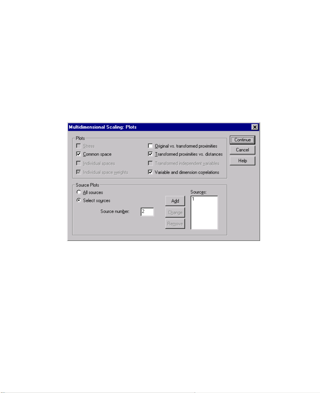
78 Chapter 7
Multidimensional Scaling Plots, Version 2
The Plots dialog box allows you to specify which plots will be produced. If your data
format is anything other than Proximities in Columns, the following Plots dialog box is
displayed. For Individual spaces weights, Original vs. transformed proximities, and
Transformed proximities vs. distances plots, you may specify the sources for which the
plots should be produced. The source numbers entered must be values of the sources
variable specified in the main dialog box, and range from 1 to the number of sources.
Figure 7.11 Multidimensional Scaling Plots dialog box, version 2
Multidimensional Scaling Output
The Output dialog box allows you to control the amount of displayed output and save
some of it to separate files.
Page 91
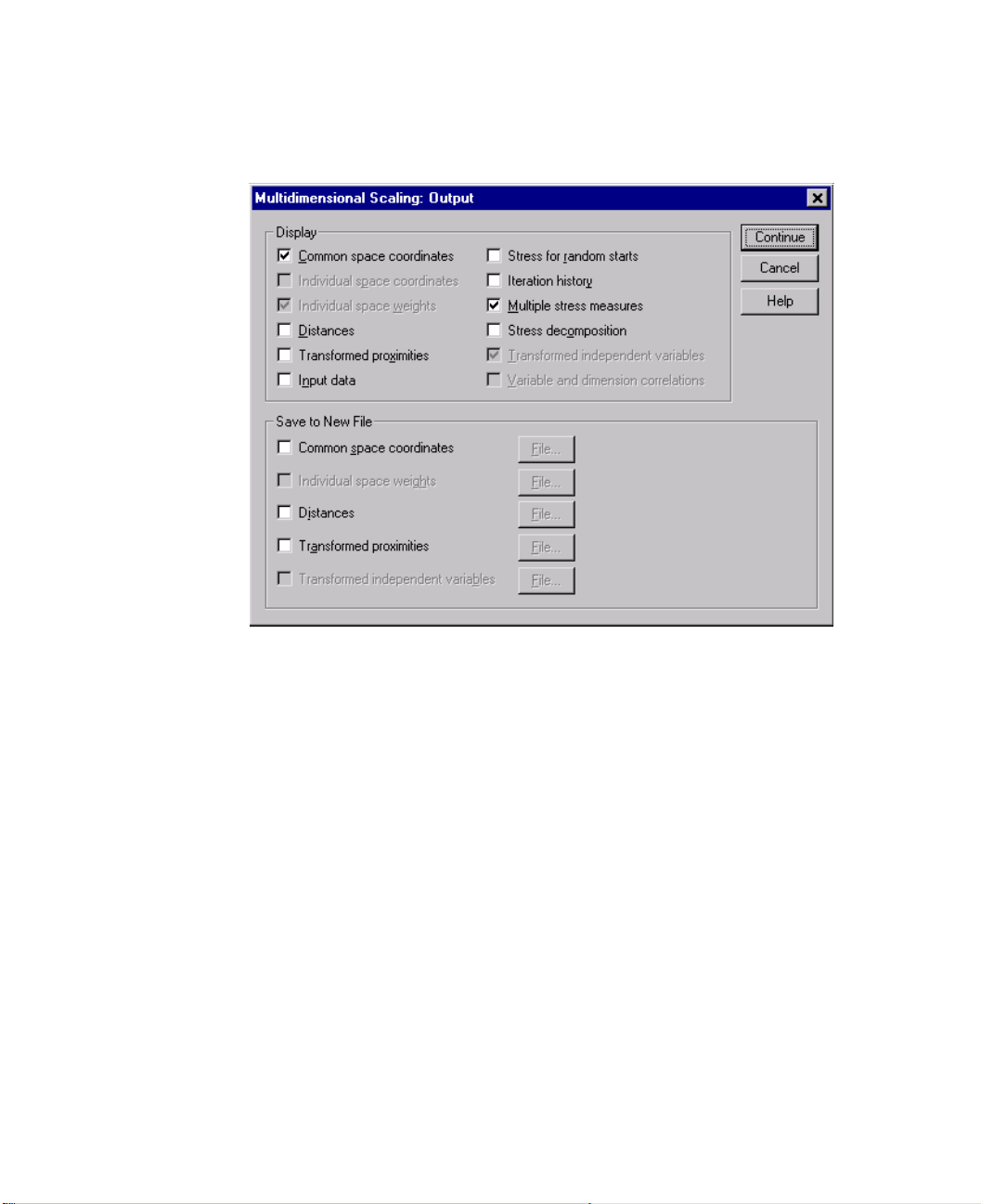
Multidimensional Scaling (PROXSCAL) 79
Figure 7.12 Multidimensional Scaling Output dialog box
Display. Select one or more of the following for display.
• Common space coordinates. Displays the coordinates of the common space.
• Individual space coordinates. The coordinates of the individual spaces are displayed,
only if the model is not the identity model.
• Individual space weights. Displays the individual space weights, only if one of the
individual differences models is specified. Depending on the model, the space
weights are decomposed in rotation weights and dimension weights, which are also
displayed.
• Distances. Displays the distances between the objects in the configuration.
• Transformed proximities. Displays the transformed proximities between the objects
in the configuration.
• Input data. Includes the original proximities, and, if present, the data weights, the ini-
tial configuration, and the fixed coordinates or the independent variables.
• Stress for random starts. Displays the random number seed and normalized raw
Stress value of each random start.
• Iteration history. Displays the history of iterations of the main algorithm.
Page 92

80 Chapter 7
• Multiple stress measures. Displays different Stress values. The table contains values
for normalized raw Stress, Stress-I, Stress-II, S-Stress, Dispersion Accounted For
(DAF), and Tucker’s Coefficient of Congruence.
• Stress decomposition. Displays an objects and sources decomposition of the final
normalized raw Stress, including the average per object and the average per source.
• Transformed independent variables. If a linear combination of independent variables
restriction was selected, the transformed independent variables and the corresponding regression weights are displayed.
• Variable and dimension correlations. If a linear combination restriction was select-
ed, the correlations between the independent variables and the dimensions of the
common space are displayed.
Save to New File. You can save the common space coordinates, individual space
weights, distances, transformed proximities, and transformed independent variables to
separate SPSS data files.
PROXSCAL Command Additional Features
You can customize your multidimensional scaling of proximities analysis if you paste
your selections into a syntax window and edit the resulting
tax. SPSS command language also allows you to:
• Specify separate variable lists for transformations and residuals plots (with the
subcommand).
• Specify separate source lists for individual space weights, transformations, and residuals plots (with the
• Specify a subset of the independent variables transformation plots to be displayed
(with the
PLOT subcommand).
PLOT subcommand).
PROXSCAL command syn-
PLOT
Page 93

Categorical Regression Examples
8
The goal of categorical regression with optimal scaling is to describe the relationship
between a response and a set of predictors. By quantifying this relationship, values of
the response can be predicted for any combination of predictors.
In this chapter, two examples serve to illustrate the analyses involved in optimal
scaling regression. The first example uses a small data set to illustrate the basic concepts. The second example uses a much larger set of variables and observations in a
practical example.
Example 1: Carpet Cleaner Data
In a popular example by Green and Wind (1973), a company interested in marketing a
new carpet cleaner wants to examine the influence of five factors on consumer preference—package design, brand name, price, a Good Housekeeping seal, and a money-
back guarantee. There are three factor levels for package design, each one differing in
the location of the applicator brush; three brand names (K2R, Glory, and Bissell); three
price levels; and two levels (either no or yes) for each of the last two factors. Table 8.1
displays the variables used in the carpet-cleaner study, with their variable labels and
values.
Table 8.1 Explanatory variables in the carpet-cleaner study
Variable label Value labels
package
brand
price
seal
money
Ten consumers rank 22 profiles defined by these factors. The variable pref contains the
rank of the average rankings for each profile. Low rankings correspond to high
preference. This variable reflects an overall measure of preference for each profile.
Using categorical regression, you will explore how the five factors in Table 8.1 are
related to preference. This data set can be found in
Package design A*, B*, C*
Brand name K2R, Glory, Bissell
Price $1.19, $1.39, $1.59
Good Housekeeping seal No, yes
Money-back guarantee No, yes
carpet.sav.
81
Page 94

82 Chapter 8
A Standard Linear Regression Analysis
To produce standard linear regression output, from the menus choose:
Analyze
Regression
Linear...
Dependent:
Independent(s): package, brand, price, seal, money
Statistics...
Descriptives (deselect)
Save...
Residuals
; Standardized
pref
The standard approach for describing the relationships in this problem is linear regression. The most common measure of how well a regression model fits the data is R
statistic represents how much of the variance in the response is explained by the weighted
combination of predictors. The closer R
on the five predictors results in an R
2
is to 1, the better the model fits. Regressing pref
2
of 0.707, indicating that approximately 71% of the
2
. This
variance in the preference rankings is explained by the predictor variables in the linear
regression.
Figure 8.1 Model summary for standard linear regression
Model
1
Adjusted
R RSquare
.841 .707 .615 3.9981
RSquare
Std.Errorof
theEstimate
The standardized coefficients are shown in Figure 8.2. The sign of the coefficient indicates whether the predicted response increases or decreases when the predictor increases, all other predictors being constant. For categorical data, the category coding
determines the meaning of an increase in a predictor. For instance, an increase in money,
package, or seal will result in a decrease in predicted preference ranking. money is coded
1 for no money-back guarantee and 2 for money-back guarantee. An increase in money
corresponds to the addition of a money-back guarantee. Thus, adding a money-back
guarantee reduces the predicted preference ranking, which corresponds to an increased
predicted preference.
Page 95
Categorical Regression Examples 83
Figure 8.2 Regression coefficients
Standardized
Coefficients
Model
(Constant)
1
Packagedesign
Brandname
Price
GoodHousekeepingseal
Money-backguarantee
Beta
-.560 -4.015 .001
.056 .407 .689
.366 2.681 .016
-.330 -2.423 .028
-.197 -1.447 .167
t Sig.
4.352 .000
The value of the coefficient reflects the amount of change in the predicted preference
ranking. Using standardized coefficients, interpretations are based on the standard deviations of the variables. Each coefficient indicates the number of standard deviations that
the predicted response changes for a one standard deviation change in a predictor, all
other predictors remaining constant. For example, a one standard deviation change in
brand yields an increase in predicted preference of 0.056 standard deviations. The standard deviation of pref is 6.44, so pref increases by . Changes in
0.056 6.44 0.361=×
package yield the greatest changes in predicted preference.
A regression analysis should always include an examination of the residuals. To
produce residual plots, from the menus choose:
Graphs
Scatter...
Select Simple. Click Define.
Y Axis:
zre_1
X Axis: zpr_1
Then, recall the Simple Scatterplot dialog box and click Reset to clear the previous
selections.
Y Axis: zre_1
X Axis: package
The standardized residuals are plotted against the standardized predicted values in
Figure 8.3. No patterns should be present if the model fits well. Here you see a U-shape
in which both low and high standardized predicted values have positive residuals. Standardized predicted values near 0 tend to have negative residuals.
Page 96
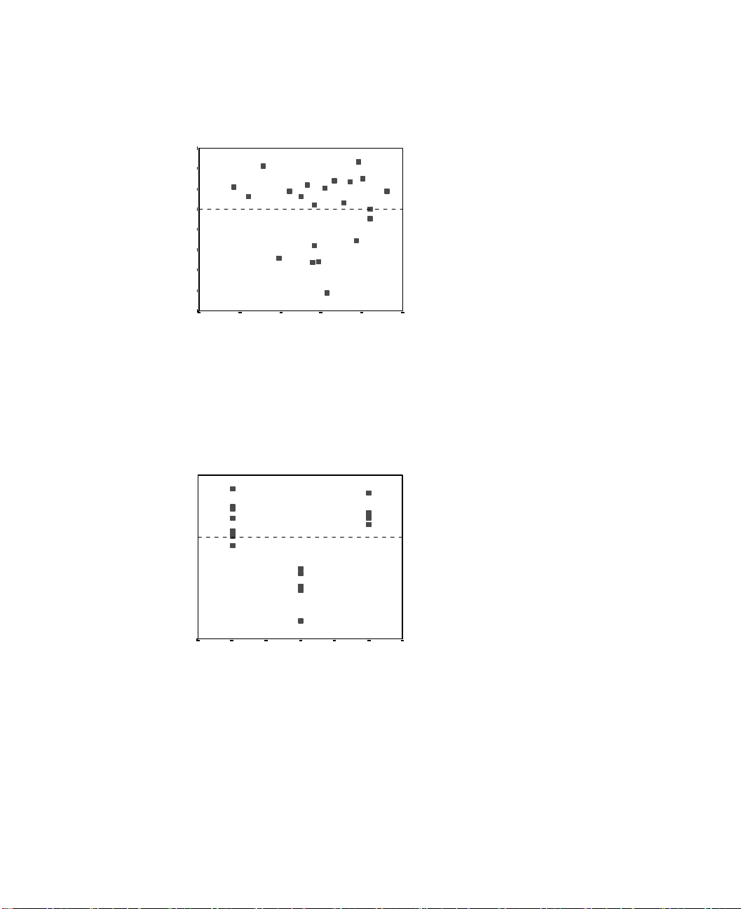
84 Chapter 8
Figure 8.3 Residuals versus predicted values
1.5
1.0
.5
0.0
-.5
-1.0
-1.5
-2.0
-2.5
StandardizedResidual
210-1-2-3
StandardizedPr e dic t ed Value
This shape is more pronounced in the plot of the standardized residuals against package
in Figure 8.4. Every residual for Design B* is negative, whereas all but one of the residuals is positive for the other two designs. Because the regression model fits one parameter for each variable, the relationship cannot be captured by the standard approach.
Figure 8.4 Residuals versus package
1.5
1.0
.5
0.0
-.5
-1.0
-1.5
-2.0
-2.5
StandardizedResidual
Pac kageDes ign
A Categorical Regression Ana lysis
The categorical nature of the variables and the nonlinear relationship between pref and
package suggest that regression on optimal scores may perform better than standard re-
gression. The U-shape of Figure 8.4 indicates that a nominal treatment of package
should be used. All other predictors will be treated at the numerical scaling level.
4332211
Page 97

Categorical Regression Examples 85
The response variable warrants special consideration. You want to predict the values
of pref. Thus, recovering as many properties of its categories as possible in the quantifications is desirable. Using an ordinal or nominal scaling level ignores the differences
between the response categories. However, linearly transforming the response categories preserves category differences. Consequently, scaling the response numerically is
generally preferred and will be employed here.
To produce the following categorical regression output, from the menus choose:
Analyze
Regression
Optimal Scaling...
Dependent:
Independent(s): package, brand, price, seal, money
Select pref. Click Define Scale.
Optimal Scaling Level
~ Numeric
Select
Optimal Scaling Level
~ Nominal
Select brand, price, seal, and money. Click Define Scale.
Optimal Scaling Level
~ Numeric
Output...
Display
; Correlations of original predictors
; Correlations of transformed predictors
Frequencies (deselect)
ANOVA table (deselect)
Save...
Save to Working File
; Transformed variables
; Residuals
Plots...
Transformation Plots:
pref
package. Click Define Scale.
package, price
Page 98
86 Chapter 8
Intercorrelations
The intercorrelations among the predictors are useful for identifying multicollinearity in
the regression. Variables that are highly correlated will lead to unstable regression estimates. However, due to their high correlation, omitting one of them from the model only
minimally affects prediction. The variance in the response that can be explained by the
omitted variable is still explained by the remaining correlated variable. However, zeroorder correlations are sensitive to outliers and also cannot identify multicollinearity due
to a high correlation between a predictor and a combination of other predictors.
Figure 8.5 and Figure 8.6 show the intercorrelations of the predictors for both the
untransformed and transformed predictors. All values are near 0, indicating that multicollinearity between individual variables is not a concern.
Notice that the only correlations that change involve package. Because all other predictors are treated numerically, the differences between the categories and the order of
the categories are preserved for these variables. Consequently, the correlations cannot
change.
Figure 8.5 Original predictor correlations
Packagedesign
Brandname
Price
Good
Housekeeping
seal
Money-back
guarantee
Package
design
1.000 -.189 -.126 .081 .066
-.189 1.000 .065 -.042 -.034
-.126 .065 1.000 .000 .000
.081 -.042 .000 1.000 -.039
.066 -.034 .000 -.039 1.000
Brand
name
Price
Figure 8.6 Transformed predictor correlations
Packagedesign
Brandname
Price
Good
Housekeeping
seal
Money-back
guarantee
Package
design
1.000 -.156 -.089 .032 .102
-.156 1.000 .065 -.042 -.034
-.089 .065 1.000 .000 .000
.032 -.042 .000 1.000 -.039
.102 -.034 .000 -.039 1.000
Brand
name
Price
Good
Housekeeping
seal
Good
Housekeeping
seal
Money-back
guarantee
Money-back
guarantee
Page 99
Categorical Regression Examples 87
Model Fit and Coefficients
2
The Categorical Regression procedure yields an R
of 0.948, indicating that almost 95%
of the variance in the transformed preference rankings is explained by the regression on
the optimally transformed predictors. Transforming the predictors improves the fit over
the standard approach.
Figure 8.7 Model summary for categorical regression
MultipleR RSquare
.974 .948 .932
Adjusted
RSquare
Figure 8.8 shows the standardized regression coefficients. Categorical regression standardizes the variables, so only standardized coefficients are reported. These values are
divided by their corresponding standard errors, yielding an F test for each variable.
However, the test for each variable is contingent upon the other predictors being in the
model. In other words, the test determines if omission of a predictor variable from the
model with all other predictors present significantly worsens the predictive capabilities
of the model. These values should not be used to omit several variables at one time for
a subsequent model. Moreover, alternating least squares optimizes the quantifications,
implying that these tests must be interpreted conservatively.
Figure 8.8 Standardized coefficients for transformed predictors
Standardized
Coefficients
Packagedesign
Brandname
Price
GoodHousekeepingseal
Money-backguarantee
Beta
4.530E-02 .058 .614
Std.Error
-.748 .058 165.495
.371 .057 41.986
-.350 .057 37.702
-.159 .057 7.669
F
The largest coefficient occurs for package. A one standard deviation increase in package
yields a 0.748 standard deviation decrease in predicted preference ranking. However,
package is treated nominally, so an increase in the quantifications need not correspond
to an increase in the original category codes.
Standardized coefficients are often interpreted as reflecting the importance of each
predictor. However, regression coefficients cannot fully describe the impact of a predictor or the relationships between the predictors. Alternative statistics must be used
in conjunction with the standardized coefficients to fully explore predictor effects.
Page 100

88 Chapter 8
Correlational Analyses
To interpret the contributions of the predictors to the regression, it is not sufficient to
only inspect the regression coefficients. In addition, the correlations, partial correlations, and part correlations should be inspected. Figure 8.9 contains these correlational
measures for each variable.
The zero-order correlation is the correlation between the transformed predictor and
the transformed response. For this data, the largest correlation occurs for package. However, if you can explain some of the variation in either the predictor or the response, you
will get a better representation of how well the predictor is doing.
Figure 8.9 Zero-order, part, and partial correlations (transformed variables)
Correlations
Zero-Order Partial Part
Packagedesign
Brandname
Price
GoodHousekeepingseal
Money-backguarantee
-.816 -.955 -.733
.206 .192 .045
.441 .851 .369
-.370 -.838 -.350
-.223 -.569 -.158
Other variables in the model can confound the performance of a given predictor in predicting the response. The partial correlation coefficient removes the linear effects of
other predictors from both the predictor and the response. This measure equals the correlation between the residuals from regressing the predictor on the other predictors and
the residuals from regressing the response on the other predictors. The squared partial
correlation corresponds to the proportion of the variance explained relative to the residual variance of the response remaining after removing the effects of the other variables.
For example, in Figure 8.9, package has a partial correlation of –0.955. Removing the
effects of the other variables, package explains of the vari-
–0.955()20.91 91 %==
ation in the preference rankings. Both price and seal also explain a large portion of variance if the effects of the other variables are removed.
Figure 8.10 displays the partial correlations for the untransformed variables. All of
the partial correlations increase when optimal scores are used. In the standard approach,
package explained 50% of the variation in pref when other variable effects were
removed from both. In contrast, package explains 91% of the variation if optimal scaling
is used. Similar results occur for price and seal.
 Loading...