

Page 1

SPSS®Base
12.0 User’s Guide
Page 2

For more information about SPSS®software products, please visit our Web site at
http://www.
SPSS Inc.
233 South Wacker Drive, 11th Floor
Chicago, IL 60
Tel: (312) 651-3000
Fax: (312) 651-3668
SPSS is a regis
of SPSS Inc. for its proprietary computer software. No material describing such
software may be produced or distributed without the written permission of the
owners of the
the published materials.
The SOFTWARE and documentation are provided with RESTRICTED RIGHTS.
Use, duplica
in subdivision (c) (1) (ii) of The Rights in Technical Data and Computer Software
clause at 52.227-7013. Contractor/manufacturer is SPSS Inc., 233 South Wacker
Drive, 11th
General notice: Other product names mentioned herein are used for identification
purposes only and may be trademarks of their respective companies.
TableLook i
Windows is a registered trademark of Microsoft Corporation.
DataDirect, DataDirect Connect, INTERSOLV, and SequeLink are registered
trademarks
Portions of this product were created using LEADTOOLS © 1991-2000, LEAD
Technologies, Inc. ALL RIGHTS RESERVED.
LEAD, LEADTO
Technologies, Inc.
Portions of this product were based on the work of the FreeType Team
(http://ww
SPSS® Base 12.0 User’s Guide
Copyright © 2003 by SPSS Inc.
All rights re
Printed in the United States of America.
No part of this publication may be reproduced, stored in a retrieval system, or
transmitted
recording, or otherwise, without the prior written permission of the publisher.
spss.com or contact
606-6412
tered trademark and the other product names are the trademarks
trademark and license rights in the software and the copyrights in
tion, or disclosure by the Government is subject to restrictions as set forth
Floor, Chicago, IL 60606-6412.
s a trademark of SPSS Inc.
of DataDirect Technologies.
OLS, and LEADVIEW are registered trademarks of LEAD
w.freetype.org).
served.
, in any form or by any means, electronic, mechanical, photocopying,
Page 3

SPSS 12.0
Preface
SPSS 12.0 is a comprehensive system for analyzing data. SPSS can take data from
almost any type of file and use them to generate tabulated reports, charts and plots of
utions and trends, descriptive statistics, and complex statistical analyses.
distrib
This manual, the SPSS Base 12.0 User's Guide, documents the graphical user
interface of SPSS for Windows. Complete information about using interactive
graphic
release 12.0 of SPSS. Examples using the statistical procedures found in SPSS
Base12.0 are provided in the Help system, installed with the software. Algorithms
used in
Some extended features of the system can be accessed only via command syntax.
(Those
syntax is documented in the SPSS 12.0 Command Syntax Reference,providedon
the product CD-ROM.
scanbefoundinSPSS Interactive Graphics 10.0, which is compatible with
the statistical procedures are available on the product CD-ROM.
In addition, beneath the menus and dialog boxes, SPSS uses a command language.
features are not available in the Student Version.) Complete command
iii
Page 4

SPSS Options
The following options are available as add-on enhancements to the full (not Student
Version) SPSS Base system:
SPSS Regress
ion Models™
provides techniques for analyzing data that do not fit
traditional linear statistical models. It includes procedures for probit analysis, logistic
regression, weight estimation, two-stage least-squares regression, and general
nonlinear r
SPSS Advanced Models™ focusesontechniquesoftenusedinsophisticated
egression.
experimental and biomedical research. It includes procedures for general linear
models (GLM
), linear mixed models, variance components analysis, loglinear
analysis, ordinal regression, actuarial life tables, Kaplan-Meier survival analysis,
and basic and extended Cox regression.
s™
SPSS Table
creates a variety of presentation-quality tabular reports, including
complex stub-and-banner tables and displays of multiple response data.
SPSS Trends™ performs comprehensive forecasting and time series analyses with
multiple c
urve-fitting models, smoothing models, and methods for estimating
autoregressive functions.
SPSS Categories® performs optimal scaling procedures, including correspondence
analysis
SPSS Conjoint™ performs conjoint analysis.
SPSS CHAID™ simplifies tabular analysis of categorical data, develops predictive
models, s
.
creens out extraneous predictor variables, and produces easy-to-read tree
diagrams that segment a population into subgroups that share similar characteristics.
SPSS Exact Tests™ calculates exact p values for statistical tests when small or very
unevenl
SPSS Missing Value Analysis™ describes patterns of missing data, estimates means
y distributed samples could make the usual tests inaccurate.
and other statistics, and imputes values for missing observations.
s™
SPSS Map
turns your geographically distributed data into high-quality maps with
symbols, colors, bar charts, pie charts, and combinations of themes to present not
only what is happening but where it is happening.
iv
Page 5

SPSS Complex Samples™ allows survey, market, health and public opinion
researchers, as well as social scientists who use sample survey methodology, to
incorporate
The SPSS family of products also includes applications for data entry, text analysis,
classification, neural networks, and flowcharting.
Compatibility
SPSS is designed to run on many computer systems. See the materials that came with
your system for specific information on minimum and recommended requirements.
Serial Numbers
Your serial number is your identification number with SPSS Inc. You will need
this serial number when you contact SPSS Inc. for information regarding support,
payment, o
system.
their complex sample designs into data analysis.
r an upgraded system. The serial number was provided with your Base
Customer
Service
If you hav
office, listed on the SPSS Web site at http://www.spss.com/worldwide/.Pleasehave
your serial number ready for identification.
Training Seminars
SPSS Inc. provides both public and onsite training seminars. All seminars feature
hands-on workshops. Seminars will be offered in major cities on a regular basis. For
more inf
Web site at http://www.spss.com/worldwide/.
ormation on these seminars, contact your local office, listed on the SPSS
e any questions concerning your shipment or account, contact your local
v
Page 6

Technical Support
The services of SPSS Technical Support are available to registered customers.
Customers may contact Technical Support for assistance in using SPSS products
or for instal
Technical Support, see the SPSS Web site at http://www.spss.com, or contact your
local office, listed on the SPSS Web site at http://www.spss.com/worldwide/.Be
prepared to
lation help for one of the supported hardware environments. To reach
identify yourself, your organization, and the serial number of your system.
Additional Publications
Individuals worldwide can order additional product manuals directly from SPSS
Inc. For te
800-543-2185. For telephone orders outside of North America, contact your local
office,listedontheSPSSWebsiteathttp://www.spss.com/worldwide.
The SPSS 12
prepared for publication by Prentice Hall. It contains overviews of the procedures
in the SPSS Base, plus Logistic Regression, General Linear Models, and Linear
Mixed Mod
http://www.spss.com (click
lephone orders in the United States and Canada, call SPSS Inc. at
.0 Statistical Procedures Companion, by Marija Norusis, is being
els. Further information will be available on the SPSS Web site at
Store, select your country, click Books).
Tell Us Y
Contac
ting SPSS
our Thoughts
Your com
products. We especially like to hear about new and interesting applications using
the SPSS system. Please send e-mail to [email protected], or write to SPSS Inc.,
Attn: Di
60606-6412.
If you w
our Web site at http://www.spss.com/worldwide/. We will send you a copy of our
newsletter and let you know about SPSS Inc. activities in your area.
ments are important. Please let us know about your experiences with SPSS
rector of Product Planning, 233 South Wacker Drive, 11th Floor, Chicago IL
ould like to be on our mailing list, contact one of our offices, listed on
vi
Page 7

Contents
1Overview 1
What'sNewinSPSS12.0?..................................... .2
Windows .................................................. .3
Menus.................................................... .6
StatusBar ................................................. .6
DialogBoxes ............................................... .7
VariableNamesandVariableLabelsinDialogBoxLists............... .7
DialogBoxControls .......................................... .8
SubdialogBoxes............................................. .9
SelectingVariables........................................... .9
GettingInformationaboutVariablesinDialogBoxes.................. .9
GettingInformationaboutDialogBoxControls..................... .10
BasicStepsinDataAnalysis .................................. .11
StatisticsCoach............................................ .12
FindingOutMoreaboutSPSS.................................. .12
2 Getting Help 13
UsingtheHelpTableofContents................................ .14
UsingtheHelpIndex......................................... .14
GettingHelponDialogBoxControls............................. .15
GettingHelponOutputTerms.................................. .16
UsingCaseStudies.......................................... .17
CopyingHelpTextfromaPop-UpWindow ........................ .17
vii
Page 8

3 Data Files 19
peningaDataFile ......................................... .19
O
oOpenDataFiles.......................................... .19
T
ataFileTypes............................................. .20
D
peningFileOptions......................................... .21
O
eadingExcelFiles.......................................... .21
R
w the Data Editor Reads Olde r Excel Files and Other Spre adsh eets . . . . 22
Ho
wtheDataEditorReadsdBASEFiles.......................... .22
Ho
adingDatabaseFiles ...................................... .23
Re
lectingaDataSource...................................... .24
Se
tabaseLogin............................................. .26
Da
lectingDataFields........................................ .26
Se
eatingaParameterQuery................................... .34
Cr
iningVariables(DatabaseWizard)............................ .35
Def
ults .................................................. .36
Res
tWizard ............................................... .37
Tex
eInformation............................................. .48
Fil
ingDataFiles ........................................... .48
Sav
aveModifiedDataFiles................................... .48
To S
ingDataFilesinExcelFormat............................... .49
Sav
ngDataFilesinSASFormat................................ .50
Savi
ngDataFilesinOtherFormats.............................. .52
Savi
ngData:DataFileTypes................................... .52
Savi
ngSubsetsofVariables................................... .54
Savi
ngFileOptions.......................................... .55
Savi
ectingOriginalData...................................... .55
Prot
viii
Page 9

VirtualActiveFile........................................... .55
4 Distributed Analysis Mode 61
DistributedversusLocalAnalysis............................... .61
5 Data Editor 73
DataView................................................. .73
VariableView.............................................. .74
EnteringData.............................................. .86
EditingData............................................... .88
GotoCase................................................ .92
CaseSelectionStatusintheDataEditor.......................... .93
DataEditorDisplayOptions.................................... .93
DataEditorPrinting.......................................... .93
6 Data Preparation 95
DefiningVariableProperties................................... .96
CopyingDataProperties..................................... .103
IdentifyingDuplicateCases .................................. .113
VisualBander............................................. .116
BandingVariables ......................................... .118
AutomaticallyGeneratingBandedCategories..................... .121
CopyingBandedCategories.................................. .124
User-MissingValuesintheVisualBander........................ .125
ix
Page 10

7 Data Transformations 127
omputingVariables........................................ .127
C
unctions................................................ .130
F
issingValuesinFunctions.................................. .131
M
andomNumberSeed ...................................... .131
R
ountOccurrencesofValueswithinCases....................... .132
C
codingValues........................................... .134
Re
codeintoSameVariables.................................. .134
Re
codeintoDifferentVariables ............................... .137
Re
nkCases............................................... .140
Ra
tomaticRecode ......................................... .144
Au
meSeriesDataTransformations.............................. .145
Ti
8Fi
le Handling and File Transformations 153
SortCases............................................... .153
Transpose................................................ .154
MergingDataFiles......................................... .155
x
Page 11

AddCases............................................... .155
AddVariables............................................. .159
AggregateData ........................................... .162
SplitFile................................................. .165
SelectCases ............................................. .166
WeightCases............................................. .171
RestructuringData......................................... .173
9 Working with Output 197
iewer.................................................. .197
V
singOutputinOtherApplications............................. .206
U
astingObjectsintotheViewer ............................... .209
P
asteSpecial............................................. .210
P
stingObjectsfromOtherApplicationsintotheViewer............. .210
Pa
portOutput............................................. .210
Ex
ewerPrinting............................................ .220
Vi
vingOutput............................................. .227
Sa
10 Dr
aft Viewer 229
ToCreateDraftOutput ...................................... .230
xi
Page 12

Controlling Draft Output Format. . . . . . . . . . . . . . . . . . . . . . . . . . . . . . . . . 231
FontsinDraftOutput........................................ .236
ToPrintDraftOutput........................................ .236
ToSaveDraftViewerOutput.................................. .237
11 Pivot Tables 239
anipulatingaPivotTable................................... .239
M
orkingwithLayers........................................ .244
W
ookmarks............................................... .248
B
howingandHidingCells.................................... .249
S
ditingResults............................................ .251
E
hangingtheAppearanceofTables............................ .251
C
ableProperties........................................... .254
T
ChangePivotTableProperties.............................. .254
To
bleProperties:General.................................... .255
Ta
ChangeGeneralTableProperties............................ .255
To
bleProperties:Footnotes .................................. .256
Ta
ChangeFootnoteMarkerProperties.......................... .256
To
bleProperties:CellFormats ................................ .257
Ta
ChangeCellFormats ..................................... .258
To
leProperties:Borders.................................... .258
Tab
hangeBordersinaTable................................. .259
To C
isplayHiddenBordersinaPivotTable....................... .260
To D
leProperties:Printing.................................... .260
Tab
ontrolPivotTablePrinting ................................ .260
To C
t.................................................... .261
Fon
aCellWidths........................................... .262
Dat
Properties............................................ .263
Cell
xii
Page 13

ToChangeCellProperties.................................... .263
CellProperties:Value....................................... .264
ToChangeValueFormatsinaCell.............................. .264
ToChangeValueFormatsforaColumn.......................... .264
CellProperties:Alignment ................................... .265
ToChangeAlignmentinCells ................................. .265
CellProperties:Margins..................................... .266
ToChangeMarginsinCells................................... .266
CellProperties:Shading..................................... .267
ToChangeShadinginCells................................... .267
FootnoteMarker........................................... .267
SelectingRowsandColumnsinPivotTables...................... .268
ToSelectaRoworColumninaPivotTable....................... .269
ModifyingPivotTableResults................................. .269
PrintingPivotTables........................................ .270
ToPrintHiddenLayersofaPivotTable.......................... .270
Controlling Table Breaks for Wide and Long Tables . . . . . . . . . . . . . . . . . . 271
12 Working with Command Syntax 273
ntaxRules.............................................. .274
Sy
tingSyntaxfromDialogBoxes ............................. .275
Pas
yingSyntaxfromtheOutputLog............................ .276
Cop
tingSyntaxinaJournalFile................................ .278
Edi
unCommandSyntax..................................... .279
To R
tipleExecuteCommands.................................. .280
Mul
xiii
Page 14

13 Frequencies 283
requenciesDataConsiderations.............................. .283
F
ampleOutput............................................ .284
S
oObtainFrequencyTables .................................. .285
T
14D
escriptives 291
DescriptivesDataConsiderations.............................. .291
SampleOutput............................................ .292
ToObtainDescriptiveStatistics ............................... .292
15 Explore 297
ExploreDataConsiderations.................................. .298
SampleOutput............................................ .298
ToExploreYourData........................................ .299
16 Crosstabs 305
CrosstabsDataConsiderations................................ .306
SampleOutput............................................ .307
xiv
Page 15

ToObtainCrosstabulations................................... .307
17 Summarize 315
SummarizeDataConsiderations............................... .315
SampleOutput............................................ .316
ToObtainCaseSummaries................................... .316
18 Means 323
MeansDataConsiderations.................................. .323
SampleOutput............................................ .324
ToObtainSubgroupMeans................................... .325
19 OLAP Cubes 329
OLAPCubesDataConsiderations.............................. .329
SampleOutput............................................ .330
ToObtainOLAPCubes ...................................... .330
20 T Tests 337
Independent-SamplesTTest.................................. .337
Independent-SamplesTTestDataConsiderations ................. .338
SampleOutput............................................ .338
ToObtainanIndependent-SamplesTTest ....................... .339
Paired-SamplesTTest...................................... .341
xv
Page 16

Paired-SamplesTTestDataConsiderations...................... .342
SampleOutput............................................ .342
ToObtainaPaired-SamplesTTest............................. .343
One-SampleTTest......................................... .344
One-SampleTTestDataConsiderations......................... .345
SampleOutput............................................ .345
ToObtainaOne-SampleTTest................................ .346
21 One-Way ANOVA 349
ne-WayANOVADataConsiderations.......................... .350
O
ampleOutput............................................ .350
S
oObtainaOne-WayAnalysisofVariance....................... .351
T
22G
LM Univariate Analysis 359
GLMUnivariateDataConsiderations ........................... .360
SampleOutput............................................ .361
ToObtainGLMUnivariateTables .............................. .362
GLMContrasts............................................ .365
GLMProfilePlots.......................................... .367
GLMPostHocComparisons.................................. .368
23 Bivariate Correlations 377
BivariateCorrelationsDataConsiderations....................... .377
SampleOutput............................................ .378
xvi
Page 17

ToObtainBivariateCorrelations............................... .379
24 Partial Correlations 383
PartialCorrelationsDataConsiderations......................... .383
SampleOutput............................................ .384
ToObtainPartialCorrelations................................. .384
25 Distances 387
ToObtainDistanceMatrices.................................. .387
DistancesDissimilarityMeasures.............................. .389
DistancesSimilarityMeasures................................ .390
26 Linear Regression 391
LinearRegressionDataConsiderations.......................... .391
SampleOutput............................................ .392
ToObtainaLinearRegressionAnalysis.......................... .394
LinearRegressionVariableSelectionMethods.................... .396
LinearRegressionSetRule................................... .397
LinearRegressionPlots ..................................... .398
LinearRegression:SavingNewVariables........................ .399
LinearRegressionStatistics.................................. .402
LinearRegressionOptions ................................... .404
xvii
Page 18

27 Curve Estimation 407
urveEstimationDataConsiderations .......................... .407
C
ampleOutput............................................ .408
S
oObtainaCurveEstimation.................................. .409
T
28D
iscriminant Analysis 413
SampleOutput............................................ .414
ToObtainaDiscriminantAnalysis.............................. .415
29 Factor Analysis 423
FactorAnalysisDataConsiderations............................ .424
SampleOutput............................................ .425
ToObtainaFactorAnalysis................................... .428
FactorAnalysisDescriptives.................................. .430
To Specify Descriptive Statistics and Correlation Coefficients . . . . . . . . . . 431
ToSpecifyExtractionOptions................................. .433
ToSpecifyRotationOptions .................................. .434
ToSpecifyFactorScoreOptions............................... .436
ToSpecifyFactorAnalysisOptions............................. .436
xviii
Page 19

30 Choosing a Procedure for Clustering 437
31 TwoStep Clu
TwoStepClusterAnalysisDataConsiderations.................... .441
ToObtainaTwoStepClusterAnalysis........................... .442
TwoStepClusterAnalysisOptions.............................. .443
TwoStepClusterAnalysisPlots................................ .446
TwoStepClusterAnalysisOutput .............................. .447
ster Analysis 439
32 Hierarchical Cluster Analysis 449
HierarchicalClusterAnalysisDataConsiderations................. .449
SampleOutput............................................ .450
ToObtainaHierarchicalClusterAnalysis........................ .451
HierarchicalClusterAnalysisStatistics.......................... .454
HierarchicalClusterAnalysisPlots............................. .455
HierarchicalClusterAnalysisSaveNewVariables................. .455
33 K-Means Cluster Analysis 457
K-MeansClusterAnalysisDataConsiderations.................... .457
SampleOutput............................................ .458
ToObtainaK-MeansClusterAnalysis........................... .460
K-MeansClusterAnalysisSave ............................... .462
K-MeansClusterAnalysisOptions ............................. .463
xix
Page 20

34 Nonparametric Tests 465
hi-SquareTest ........................................... .466
C
hi-SquareTestDataConsiderations ........................... .466
C
ampleOutput............................................ .467
S
oObtainaChi-SquareTest.................................. .468
T
inomialTest............................................. .471
B
nomialTestDataConsiderations............................. .471
Bi
mpleOutput............................................ .472
Sa
ObtainaBinomialTest.................................... .472
To
nsTest................................................ .474
Ru
nsTestDataConsiderations................................ .475
Ru
mpleOutput............................................ .475
Sa
ObtainaRunsTest....................................... .475
To
-SampleKolmogorov-SmirnovTest.......................... .478
One
-Sample Kolmogorov-Smirnov Test Data Considerations . . . . . . . . . . . 478
One
pleOutput............................................ .479
Sam
btainaOne-SampleKolmogorov-SmirnovTest................. .479
To O
-Independent-SamplesTests.............................. .481
Two
-Independent-Samples Tests Data Considerations . . . . . . . . . . . . . . . 482
Two
pleOutput............................................ .482
Sam
tainTwo-Independent-SamplesTests....................... .483
To O b
Related-SamplesTests.................................. .487
Two-
Related-SamplesTestsDataConsiderations.................. .487
Two-
leOutput............................................ .487
Samp
tainTwo-Related-SamplesTests .......................... .488
To O b
sforSeveralIndependentSamples ......................... .490
Test
s for Several Independent Samples Data Considerations . . . . . . . . . . 491
Test
leOutput............................................ .491
Samp
xx
Page 21

ToObtainTestsforSeveralIndependentSamples.................. .492
TestsforSeveralRelatedSamples ............................. .495
TestsforSeveralRelatedSamplesDataConsiderations............. .495
SampleOutput............................................ .495
ToObtainTestsforSeveralRelatedSamples...................... .496
35 Multiple Response Analysis 499
ultipleResponseDefineSets................................ .500
M
oDefineMultipleResponseSets.............................. .501
T
ultipleResponseFrequencies............................... .502
M
ultiple Response Frequencies Data Considerations . . . . . . . . . . . . . . . . 503
M
ampleOutput............................................ .503
S
oObtainMultipleResponseFrequencies........................ .504
T
ltipleResponseCrosstabs................................. .504
Mu
ltipleResponseCrosstabsDataConsiderations................. .505
Mu
mpleOutput............................................ .506
Sa
ObtainMultipleResponseCrosstabs ......................... .506
To
36 Re
porting Results 511
ReportSummariesinRows................................... .511
ReportSummariesinColumns ................................ .519
37 Reliability Analysis 527
Reliability Analysis Data Considerations . . . . . . . . . . . . . . . . . . . . . . . . . . 528
xxi
Page 22

SampleOutput............................................ .528
To Obtain a Reliability Analysis . . . . . . . . . . . . . . . . . . . . . . . . . . . . . . . . . 529
RELIABILITYCommandAdditionalFeatures ...................... .532
38 Multidimensional Scaling 533
MultidimensionalScalingDataConsiderations.................... .534
oObtainaMultidimensionalScalingAnalysis.................... .534
T
ultidimensionalScalingCreateMeasure....................... .536
M
ultidimensionalScalingModel............................... .537
M
ultidimensionalScalingOptions.............................. .538
M
calingCommandAdditionalFeatures.......................... .539
S
39R
atio Statistics 541
RatioStatisticsDataConsiderations............................ .541
ToObtainRatioStatistics .................................... .542
RatioStatisticsStatistics .................................... .543
xxii
Page 23

40 Overview of the Chart Facility 545
reatingandModifyingaChart................................ .545
C
hartDefinitionGlobalOptions................................ .550
C
41R
OC Curves 557
ROCCurveDataConsiderations ............................... .557
SampleOutput............................................ .558
ToObtainanROCCurve ..................................... .559
42 Utilities 561
VariableInformation........................................ .561
DataFileComments........................................ .562
VariableSets ............................................. .563
DefineVariableSets........................................ .563
UseSets................................................. .564
ReorderingTargetVariableLists............................... .565
43 Options 567
GeneralOptions........................................... .568
ViewerOptions............................................ .570
DraftViewerOptions ....................................... .571
xxiii
Page 24

OutputLabelOptions ....................................... .573
ChartOptions............................................. .575
InteractiveChartOptions .................................... .579
PivotTableOptions......................................... .581
DataOptions.............................................. .582
CurrencyOptions.......................................... .583
ScriptOptions............................................. .585
44 Customizing Menus and Toolbars 587
enuEditor.............................................. .587
M
ustomizingToolbars....................................... .588
C
howToolbars............................................ .588
S
oCustomizeToolbars ...................................... .589
T
45P
roduction Facility 595
Using the Production Facility . . . . . . . . . . . . . . . . . . . . . . . . . . . . . . . . . . 596
Syntax Rules for the Production Facility . . . . . . . . . . . . . . . . . . . . . . . . . . 596
ExportOptions ............................................ .597
UserPrompts............................................. .600
ProductionMacroPrompting................................. .602
ProductionOptions......................................... .602
FormatControlforProductionJobs............................. .603
RunningProductionJobsfromaCommandLine................... .606
PublishtoWeb............................................ .607
SmartViewerWebServerLogin ............................... .608
xxiv
Page 25

46 SPSS Scripting Facility 609
oRunaScript............................................ .609
T
criptsIncludedwithSPSS .................................. .610
S
utoscripts............................................... .611
A
reatingandEditingScripts.................................. .612
C
oEditaScript............................................ .613
T
riptWindow............................................ .614
Sc
arterScripts............................................ .617
St
eatingAutoscripts........................................ .618
Cr
wScriptsWork.......................................... .622
Ho
bleofObjectClassesandNamingConventions.................. .624
Ta
wProcedure(Scripting)................................... .629
Ne
dingaDescriptiontoaScript............................... .632
Ad
xxv
Page 26

ScriptingCustomDialogBoxes................................ .632
DebuggingScripts......................................... .636
ScriptFilesandSyntaxFiles.................................. .639
47 Output Management System 643
OMSIdentifiers ........................................... .643
Appendices
A Database Access Administrator 649
B Customizing HTML Documents 651
To Add Customized HTML Code to Exported Output Documents . . . . . . . . 651
ContentandFormatoftheTextFileforCustomizedHTML............ .652
ToUseaDifferentFileorLocationforCustomHTMLCode ........... .652
Index 655
xxvi
Page 27

Overview
SPSS for Windows provides a powerful statistical analysis and data management
system in a g
to do most of the work for you. Most tasks can be accomplished simply by pointing
and clicking the mouse.
Chapter
1
raphical environment, using descriptive menus and simple dialog boxes
In additio
Windows provides:
Data Editor. A versatile spreadsheet-like system for defining, entering, editing, and
displayin
Viewer. The Viewer makes it easy to browse your results, selectively show and hide
output, change the display order results, and move presentation-quality tables and
charts be
Multidimensional pivot tables. Your results come alive with multidimensional pivot
tables. Explore your tables by rearranging rows, columns, and layers. Uncover
importan
splitting your table so that only one group is displayed at a time.
High-resolution graphics. High-resolution, full-color pie charts, bar charts, histograms,
scatter
Database access. Retrieve information from databases by using the Database Wizard
instead of complicated SQL queries.
Data tra
You can easily subset data, combine categories, add, aggregate, merge, split, and
transpose files, and more.
Electro
export tables and charts in HTML format for Internet and intranet distribution.
n to the simple point-and-click interface for statistical analysis, SPSS for
gdata.
tween SPSS and other applications.
t findings that can get lost in standard reports. Compare groups easily by
plots, 3-D graphics, and more are included as standard features in SPSS.
nsformations.
nic distribution.
Transformation features help get your data ready for analysis.
Send e-mail reports to others with the click of a button, or
1
Page 28

2
Chapter 1
Online Help. Detailed tutorials provide a comprehensive overview; context-sensitive
Help topics in dialog boxes guide you through specific tasks; pop-up definitions in
pivot table
results explain statistical terms; the Statistics Coach helps you find the
procedures that you need; and Case Studies provide hands-on examples of how to use
statistical procedures and interpret the results.
Command lan
guage.
Although most tasks can be accomplished with simple
point-and-click gestures, SPSS also provides a powerful command language that
allows you to save and automate many common tasks. The command language also
provides s
ome functionality not found in the menus and dialog boxes.
Complete command syntax documentation is automatically installed when you
install SPSS. To access the syntax documentation:
E From the menus, choose
Help
Command Sy
ntax Reference
What's New in SPSS 12.0?
There are a number of new features in SPSS 12.0.
Improved Charting Features
Better default chart appearance
Support for long text strings and automatic text wrapping
Control of default scale ranges using chart templates
3-D effects for pie and bar charts
Improved color and pattern choices, and much more
New Data Ma
Longer v
nagement Fea tures
ariable names.
The maximum length for variable names is now 64 bytes,
compared to 8 bytes for previous releases. For more information, see “Variable
Names” in Chapter 5 on page 76.
Visual Bander. The Visual Bander is designed to help you “band” scale data into
categori
cal ranges (for example, age in 10-year ranges). For more information,
see “Visual Bander” in Chapter 6 on page 116.
Page 29

Overview
Duplicate record finder. Identify, flag, report, and filter duplicate records with the
new Identif
y Duplicate Cases feature. For more information, see “Identifying
Duplicate Cases” in Chapter 6 on page 113.
Output management system. Turn output into input with the new OMS command.
OMS, you can automatically write selected categories of output to different
With
output file
s in different formats, including HTML, XML, text, and SPSS-format
data files. For more information, see “Output Management System” in Chapter
47 on page 643.
Command syntax to delete variables. The new DELETE VARIABLES command
makes it ea
sy to delete variables you do not need anymore, such as temporary
variables used in transformations.
Statistical Enhancements
New options for handling weighted data in the Crosstabs procedure. For more
informat
New stepw
ion, see “Crosstabs Cell Display” in Chapter 16 on page 313.
ise function in Multinomial Logisitic Regression (
NOMREG command,
Regression Models option).
3
New Co m plex Samples Option
This new add-on module provides the specialized planning tools and statistics that
you need when working with sample survey data. Most conventional statistical
software
surveys, however, simple random sampling generally is not feasible or cost effective.
Using SPSS Complex Samples with sample survey data reduces the risk of reaching
incorre
module enables you to make more statistically valid inferences for a population by
incorporating the sample design into survey analysis. It is an indispensable statistical
tool fo
and it enables you to reach more accurate conclusions when working with sample
survey methodology.
Windows
There are a number of different types of windows in SPSS:
assumes your data arise from simple random sampling. In most large-scale
ct or misleading inferences. The new SPSS Complex Samples add-on
r survey and market researchers, public opinion researchers or social scientists,
Page 30

4
Chapter 1
Data Editor. This window displays the contents of the data file. You can create new
data files or modify existing ones with the Data Editor. The Data Editor window
opens autom
atically when you start an SPSS session. You can have only one data
file open at a time.
Viewer. All statistical results, tables, and charts are displayed in the Viewer. You can
edit the out
put and save it for later use. A Viewer window opens automatically the
first time you run a procedure that generates output.
Draft Viewer. You can display output as simple text (instead of interactive pivot tables)
in the Draf
Pivot Table Editor. Output displayed in pivot tables can be modified in many ways with
tViewer.
the Pivot Table Editor. You can edit text, swap data in rows and columns, add color,
create mul
Chart Editor. You can modify high-resolution charts and plots in chart windows. You
tidimensional tables, and selectively hide and show results.
can change the colors, select different type fonts or sizes, switch the horizontal and
vertical
Text Output Editor. Text output not displayed in pivot tables can be modified with the
axes, rotate 3-D scatterplots, and even change the chart type.
Text Output Editor. You can edit the output and change font characteristics (type,
style, co
lor, size).
Syntax Editor. You can paste your dialog box choices into a syntax window, where
your selections appear in the form of command syntax. You can then edit the
command
syntax to use special features of SPSS not available through dialog boxes.
You can save these commands in a file for use in subsequent SPSS sessions.
Script Editor. Scripting and OLE automation allow you to customize and automate
many tas
ks in SPSS. Use the Script Editor to create and modify basic scripts.
Page 31
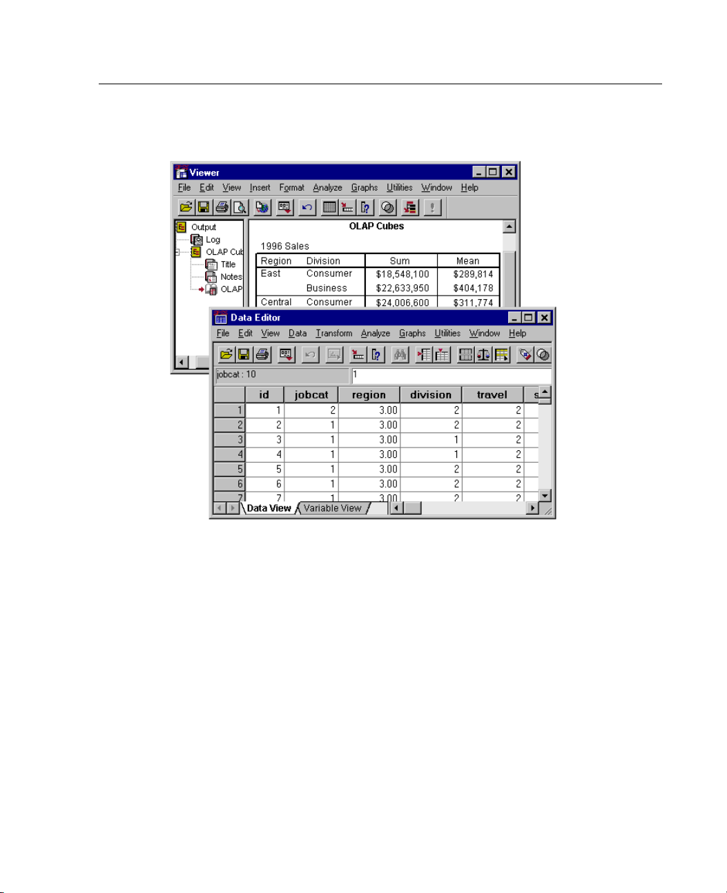
Figure 1-1
Data Editor and Viewer
5
Overview
Designated versus Active Window
If you have more than one open Viewer window, output is routed to the designated
Viewer window. If you have more than one open Syntax Editor window, command
syntax is pasted into the designated Syntax Editor window. The designated windows
are indicated by an exclamation point (!) in the status bar. You can change the
designated windows at any time.
The designated window should not be confused with the active window, which is
the currently selected window. If you have overlapping windows, the active window
appears in the foreground. If you open a new Syntax Editor or Viewer window, that
window automatically becomes the active window and the designated window.
Page 32
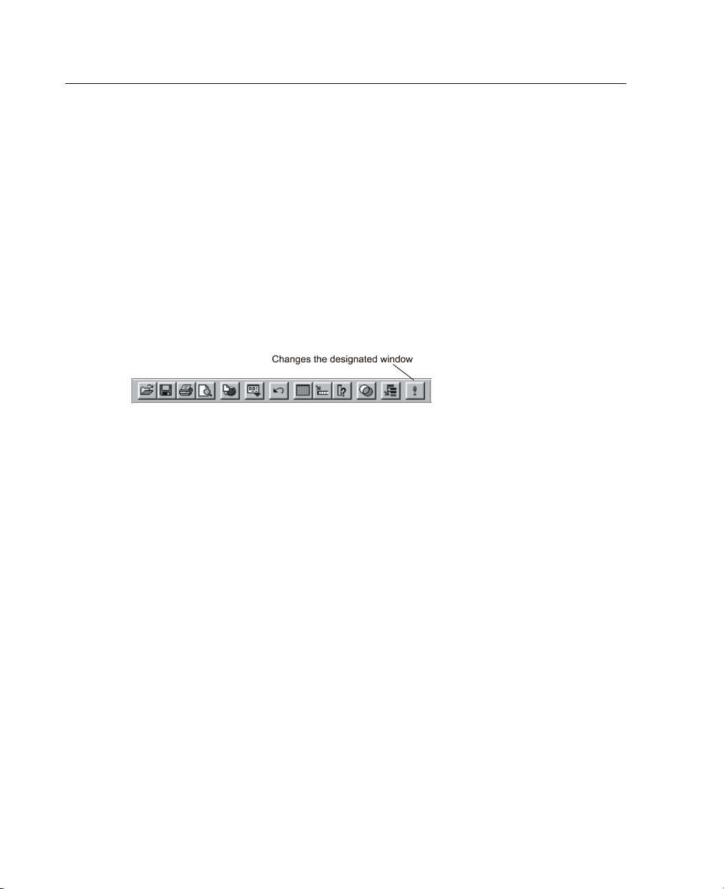
6
Chapter 1
Changing the Designated Window
E Make the window that you want to designate the active window (click anywhere
in the window).
E Click the Designate Window tool on the toolbar (the one with the exclamation point).
or
E From the menus choose:
Utilities
Designate Window
Figure 1-2
Designate Window tool
Menus
Many of the tasks that you want to perform with SPSS start with menu selections.
Each windo
that window type.
The Analyze and Graphs menus are available on all windows, making it easy to
generate n
Status Bar
The status bar at the bottom of each SPSS window provides the following information:
Command s
indicates the number of cases processed so far. For statistical procedures that require
iterative processing, the number of iterations is displayed.
Filter st
the message Filter on indicates that some type of case filtering is currently in effect
and not all cases in the data file are included in the analysis.
w in SPSS has its own menu bar with menu selections appropriate for
ew output without having to switch windows.
tatus.
For each procedure or command that you run, a case counter
atus.
If you have selected a random sample or a subset of cases for analysis,
Page 33

Overview
Weight status. The message Weight on indicates that a weight variable is being used
to weight cases for analysis.
tatus.
Split File s
separate groups for analysis, based on the values of one or more grouping variables.
The message Split File on indicates that the data file has been split into
7
Showing and
E From the me
View
Status Bar
Dialog Box
Most menu s
and options for analysis.
Dialog boxes for statistical procedures and charts typically have two basic
components:
Source var
allowed by the selected procedure are displayed in the source list. Use of short string
and long string variables is restricted in many procedures.
Tar g e t va r
for the analysis, such as dependent and independent variable lists.
Variable
Names and Variable Labels in Dialog Box Lists
Hiding the Status Bar
nus choose:
es
elections open dialog boxes. You use dialog boxes to select variables
iable list.
iable list(s).
A list of variables in the working data file. Only variable types
One or more lists indicating the variables that you have chosen
You can di
To contr
To define or modify variable labels, use Variable View in the Data Editor.
For data imported from database sources, field names are used as variable labels.
splay either variable names or variable labels in dialog box lists.
ol the display of variable names or labels, choose
menu in any window.
Options from the Edit
Page 34
8
Chapter 1
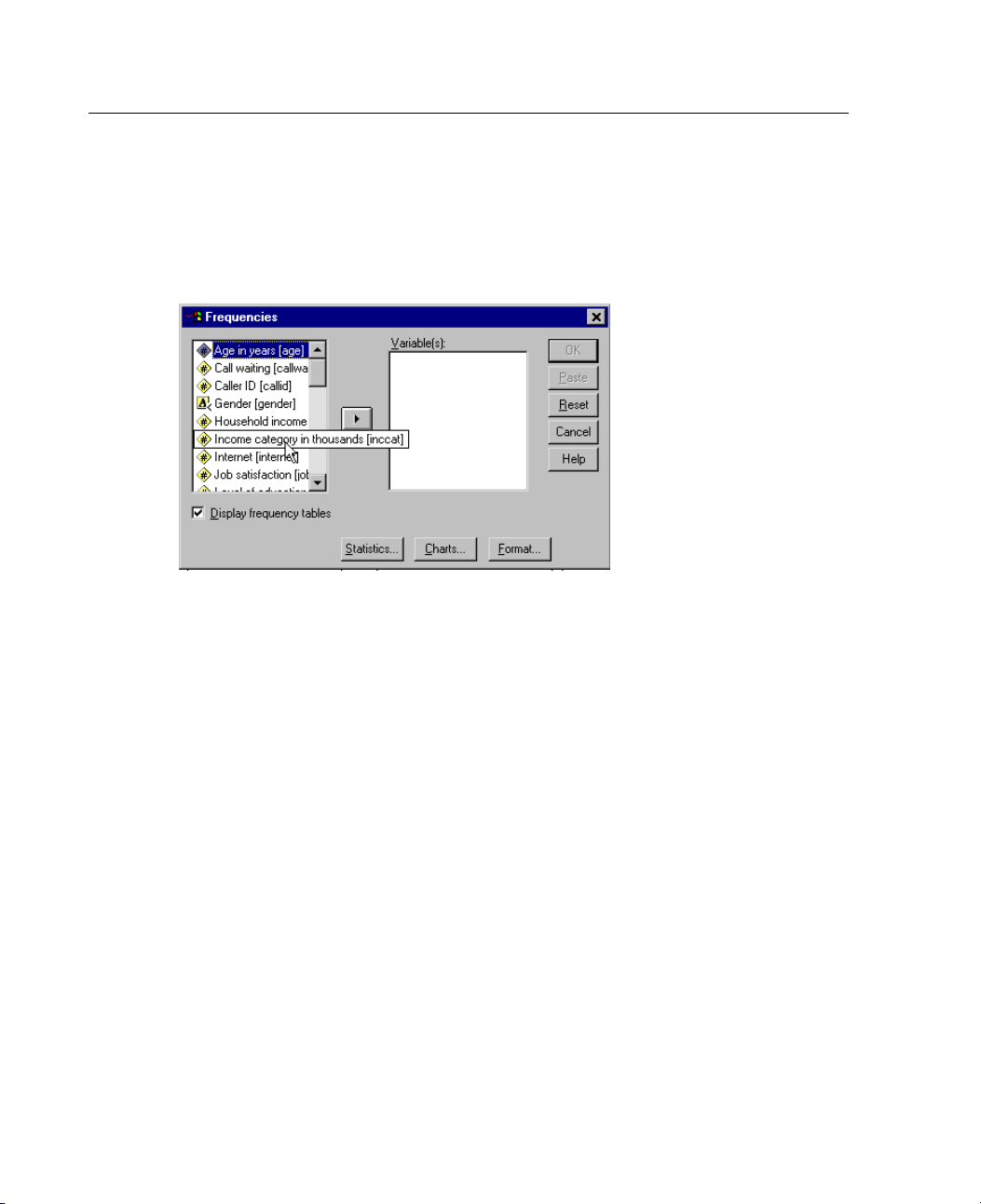
For long labels, position the mouse pointer over the label in the list to view
theentirel
If no variab
Figure 1-3
Variable labels displayed in a dialog box
abel.
le label is defined, the variable name is displayed.
Dialog Box Controls
There are five standard controls in most dialog boxes:
OK. Runs the procedure. After you select your variables and choose any additional
specifications, click
Paste. Generates command syntax from the dialog box selections and pastes the
OK to run the procedure. This also closes the dialog box.
syntax into a syntax window. You can then customize the commands with additional
features not available from dialog boxes.
Reset. Deselects any variables in the selected variable list(s) and resets all
specifications in the dialog box and any subdialog boxes to the default state.
Cancel. Cancels any changes in the dialog box settings since the last time it was
opened and closes the dialog box. Within a session, dialog box settings are persistent.
A dialog b ox retains your last set of specifications until you override them.
Help. Context-sensitive Help. This takes you to a Help window that contains
information about the current dialog box. You can also get help on individual dialog
box controls by clicking the control with the right mouse button.
Page 35

Overview
9
Subdialog Bo
Since most p
choices can be contained in a single dialog box. The main dialog box usually contains
the minimum information required to run a procedure. Additional specifications
are made in s
subdialog box will be displayed.
xes
rocedures provide a great deal of flexibility, not all of the possible
ubdialog boxes.
In the main dialog box, controls with an ellipsis (...) after the name indicate that a
Selecting Variables
To select a single variable, you simply highlight it on the source variable list and
click the right arrow button next to the target variable list. If there is only one target
variable l
list to the target list.
You can also select multiple variables:
To select multiple variables that are grouped together on the variable list, click the
To selec
ist, you can double-click individual variables to move them from the source
first one
the Ctrl-click method. Click the first variable, then Ctrl-click the next variable,
and so on.
and then Shift-click the last one in the group.
t m ultiple variables that are not grouped together on the variable list, use
Getting
E Right-
E Select
Information about Variables in Dialog Boxes
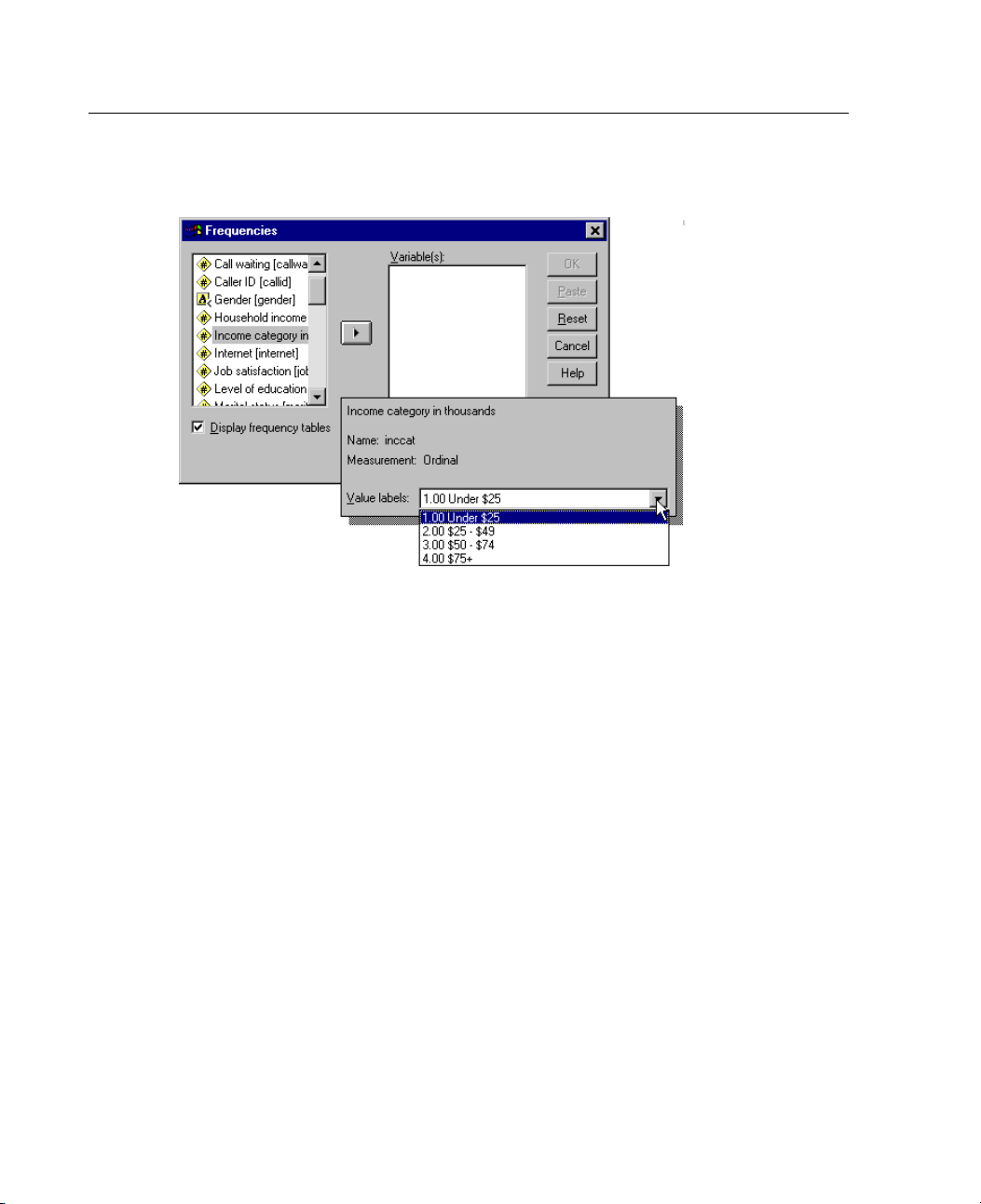
click on a variable in the source or target variable list.
Variable Information in the pop-up context menu.
Page 36
10
Chapter 1
Figure 1-4
Variable information with right mouse button
Getting Information about Dialog Box Controls
E Right-click the control you want to know about.
E Select What's This? on the pop-up context menu.
A pop-up window displays information about the control.
Page 37
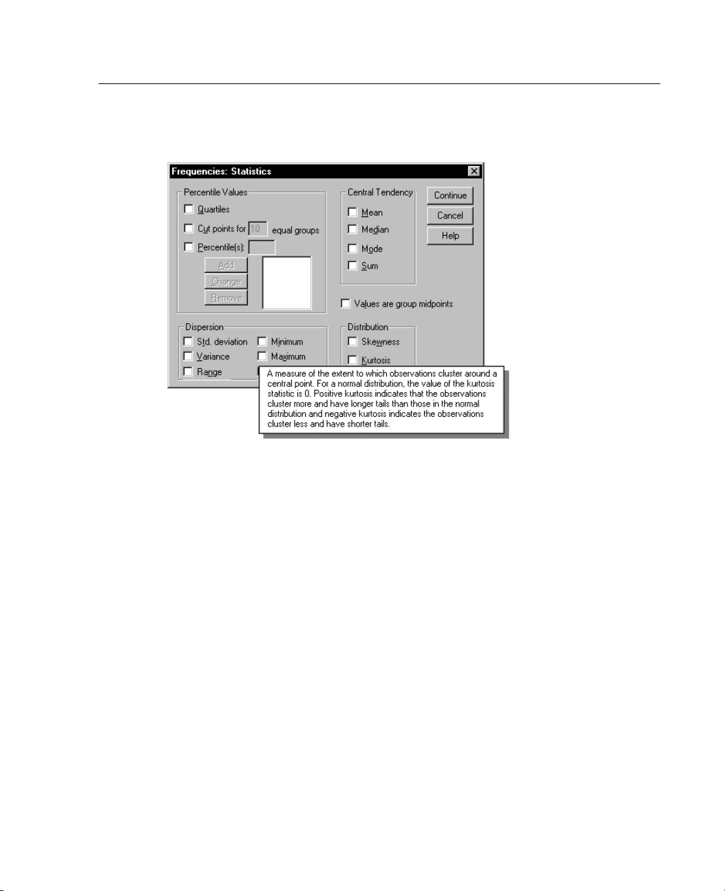
Figure 1-5
Right mouse button “What's This?” pop-up Help for dialog box controls
11
Overview
Basic Steps in Data Analysis
Analyzing data with SPSS is easy. All you have to do is:
Get your data into SPSS. You can open a previously saved SPSS data file; read a
spreadsheet, database, or text data file; or enter your data directly in the Data Editor.
Select a procedure. Select a procedure from the menus to calculate statistics or to
create a chart.
Select the variables for the analysis. Thevariablesinthedatafilearedisplayedina
dialog box for the procedure.
Run the procedure and look at the results. Results are displayed in the Viewer.
Page 38

12
Chapter 1
Statistics C
oach
If you are un
the Statistics Coach can help you get started by prompting you with simple questions,
nontechnical language, and visual examples that help you select the basic statistical
and chartin
To use the S
Help
Statistics Coach
The Statistics Coach covers only a selected subset of procedures in the SPSS Base
system. It is designed to provide general assistance for many of the basic, commonly
used stati
familiar with SPSS or with the statistical procedures available in SPSS,
g features that are best suited for your data.
tatistics Coach, from the menus in any SPSS window choose:
stical techniques.
Finding Out More about SPSS
For a comprehensive overview of SPSS basics, see the online tutorial. From any
SPSS menu
Help
Tutorial
choose:
Page 39

Getting Help
Online Help is provided in several ways:
Help menu. Every window has a Help menu on the menu bar. Topics provides access
to the Contents and Index tabs, which you can use to find specific Help topics.
provides access to the introductory tutorial.
Dialog box context m enu Help. Right-click on any control in a dialog box and select
What's This? from the context menu to display a description of the control and
directions for its use.
Dialog box Help buttons. Most dialog boxes have a Help button that takes you directly
to a Help topic for that dialog box. The Help topic provides general information and
links to related topics.
Chapter
2
Tutorial
Pivot table context menu Help. Right-click on terms in an activated pivot table in
the Viewer and select
of the terms.
Case Studies. The Case Studies item on the Help menu in the View er window provides
hands-on examples of how to create various types of statistical analyses and how to
interpret the results. The sample data files used in the examples are also provided so
that you can work through the examples to see exactly how the results were produced.
Tut o r ial. Select Tutorial on the Help menu in any window to access the online
introductory tutorial.
Command Syn tax Reference. Detailed command syntax reference information is
available in PDF format. (It is not available with some versions.)
Note: The Help system requires Internet Explorer 5 or later, and the SPSS Command
Syntax Reference requires Adobe Acrobat. Installable versions of both are provided
on the CD.
What's This? from the context menu to display definitions
13
Page 40
14
Chapter 2
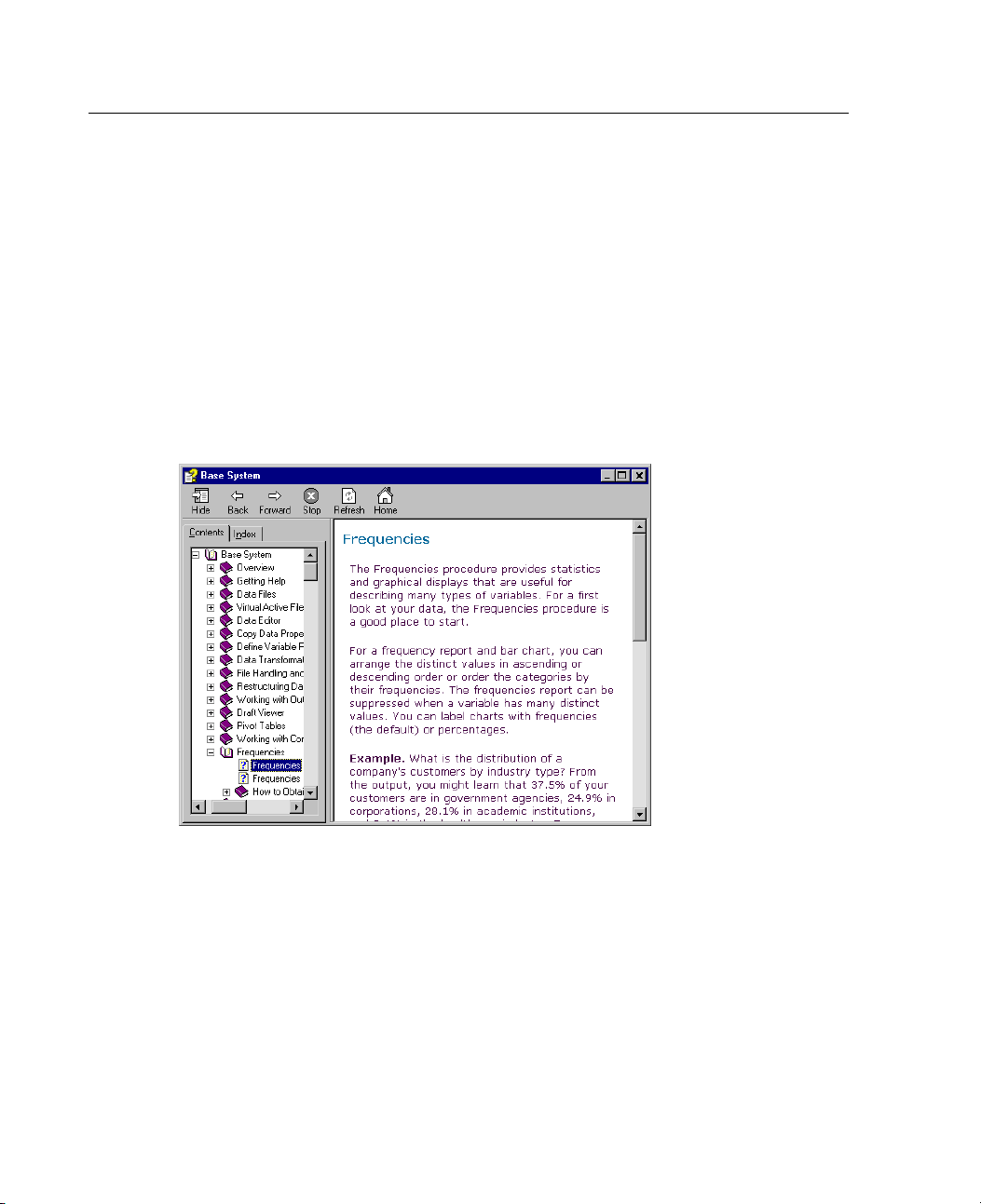
Using the Hel
E In any wind
Help
Topics
Click the Contents tab.
E
E Double-click items with a book icon to expand or collapse the contents.
E ClickanitemtogotothatHelptopic.
Figure 2-1
Help window
p Table of Contents
ow, from the menus choose:
with Contents tab displayed
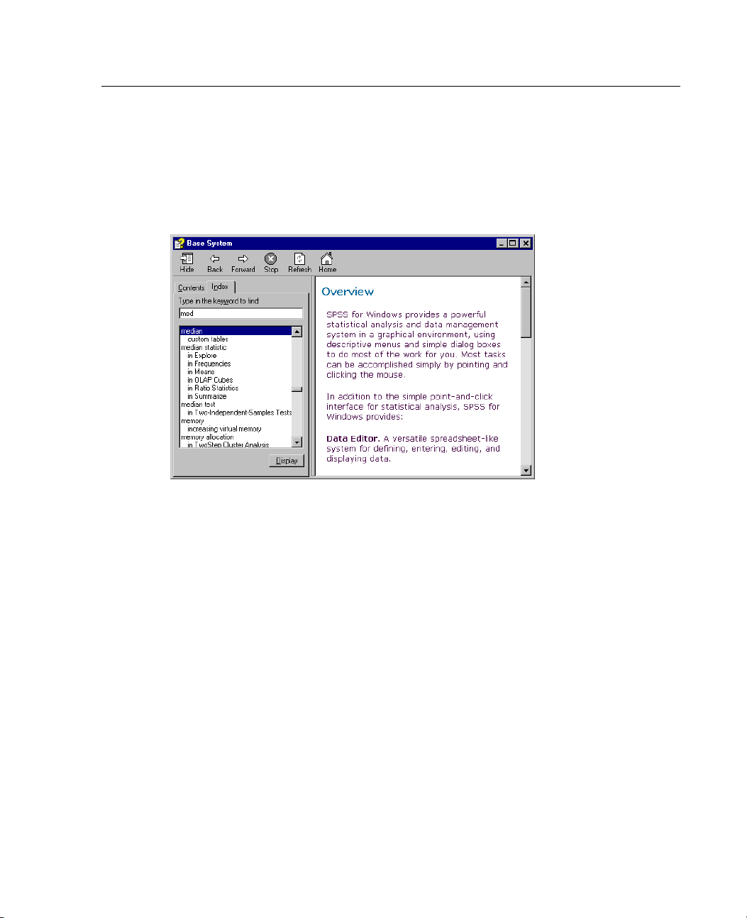
Using the Help Index
E In any window, from the menus choose:
Help
Topics
Click the Index tab.
E
E Enter a term to search for in the index.
Page 41
E
Double-click the topic that you want.
The Help index uses incremental search to find the text that you enter and selects
the closest
Figure 2-2
Index tab and incremental search
matchintheindex.
15
Getting Help
Getting Help on Dialog Box Controls
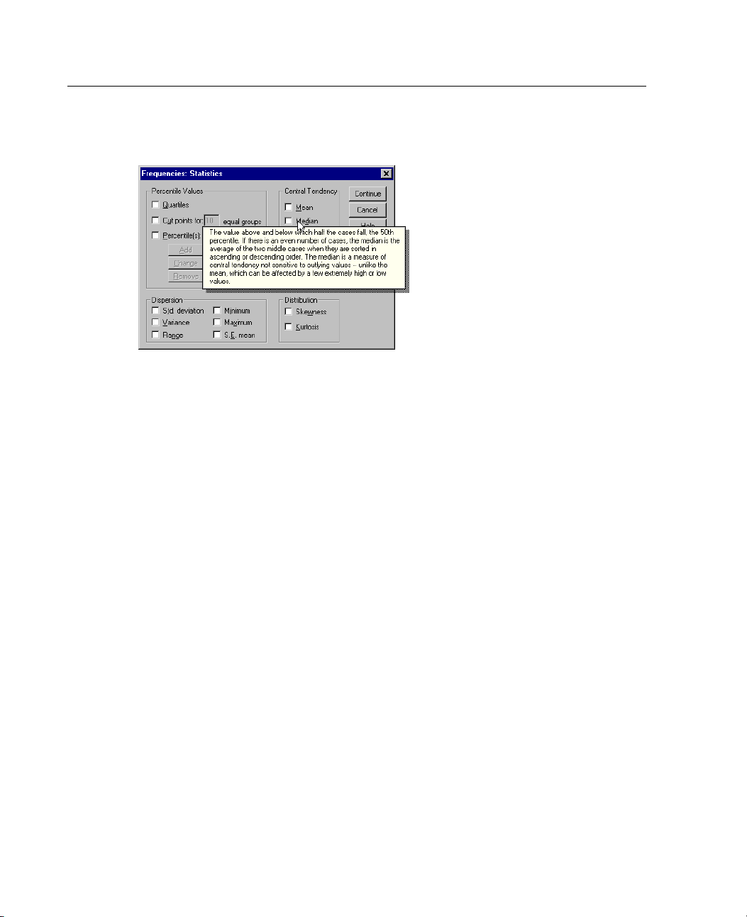
E Right-click on the dialog box control that you want information about.
E Choose What's This? from the pop-up context menu.
A descri
General information about a dialog box is available from the Help button in the
dialog box.
ption of the control and how to use it is displayed in a pop-up window.
Page 42
16
Chapter 2
Figure 2-3
Dialog box control Help with right mouse button
Getting H
E Double-
E Right-c
E Choose W
A definition of the term is displayed in a pop-up window.
elp on Output Terms
click the pivot table to activate it.
lick on the term that you want to be explained.
hat's This?
from the context menu.
Page 43
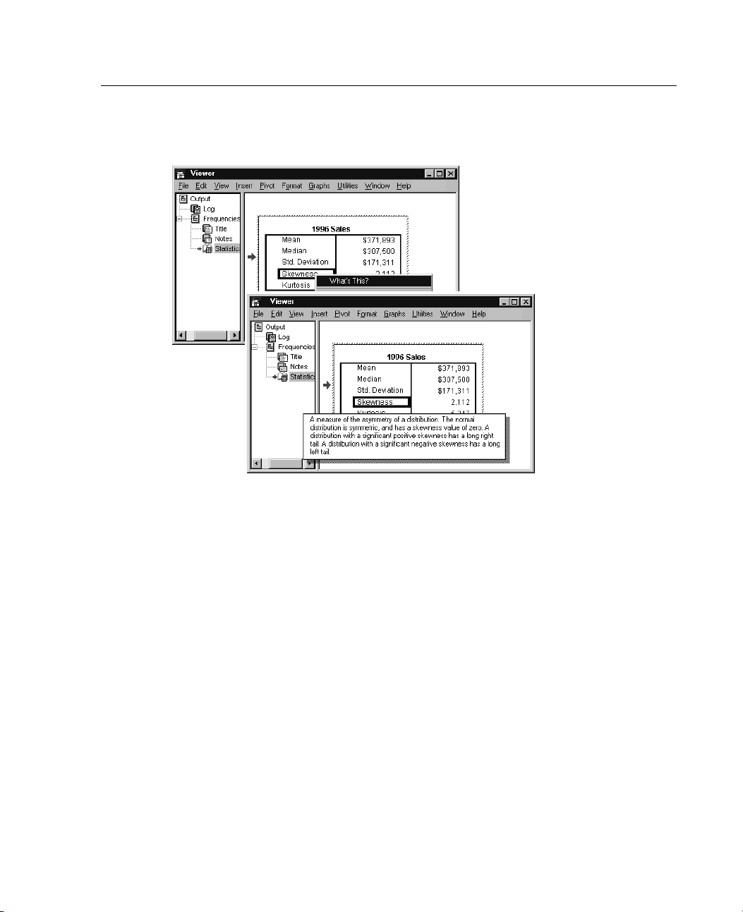
Figure 2-4
Activated pivot table glossary Help with right mouse button
17
Getting Help
UsingCaseStudies
E Right-click on a pivot table in the Viewer window.
E Choose Case Studies from the pop-up context menu.
Copying Help Text from a Pop-Up Window
E Right-click anywhere in the pop-up window.
E Choose Copy from the context menu.
The entire text of the pop-up window is copied.
Page 44

Page 45

Data Files
Data files come in a wide variety of formats, and this software is designed to handle
many of them
Spreadshe
Database f
Tab-delim
Data files
SYSTAT dat
SAS data fi
Chapter
3
, including:
ets created with Lotus 1-2-3 and Excel
iles created with dBASE and various SQL formats
ited and other types of ASCII text files
in SPSS format created on other operating systems
afiles
les
Opening a Data File
In addition to files saved in SPSS format, you can open Excel, Lotus 1-2-3, dBASE,
and tab-del
entering data definition information.
To Open Dat
E From the m
File
Open
Data...
In the Open File dialog box, select the file that you want to open.
E
E Click Open.
imited files without converting the files to an intermediate format or
a Files
enus choose:
19
Page 46

20
Chapter 3
Optionally, you can:
Read variable names from the first row for spreadsheet and tab-delimited files.
Specify a range of cells to read for spreadsheet files.
Specify a sheet within an Excel file to read (Excel 5 or later).
Data File Typ
SPSS. Opens d
Macintosh, UNIX, and also the DOS product SPSS/PC+.
SPSS/PC+. Opens SPSS/PC+ data files.
SYSTAT. Ope
SPSS Portable. Opens data files saved in SPSS portable format. Saving a file in
portable format takes considerably longer than saving the file in SPSS format.
Excel. Open
Lotus 1-2-3. Opens data files saved in 1-2-3 format for release 3.0, 2.0, or 1A of Lotus.
SYLK. Opens data files saved in SYLK (symbolic link) format, a format used by
some spread
dBASE. Opens dBASE-format files for either dBASE IV, dBASE III or III PLUS,
or dBASE II. Each case is a record. Variable and value labels and missing-value
specificat
SASLongFileName.SAS version 7-8 for Windows, long extension.
SAS Short File Name. SAS version 7-8 for Windows, short extension.
SAS v6 for Wi
es
ata files saved in SPSS format, including SPSS for Windows,
ns SYSTAT data files.
s Excel files.
sheet applications.
ions are lost when you save a file in this format.
ndows.
SAS version 6.08 for Windows and OS2.
SAS v6 for UNIX. SAS version 6 for UNIX (Sun, HP, IBM).
SAS Transport. SAS transport file.
Text. ASCII
text file.
Page 47

21
Data Files
Opening File
Read variab
of the file or the first row of the defined range. The values are converted as necessary
to create valid variable names, including converting spaces to underscores.
Worksheet.
Data Editor reads the first worksheet. To read a different worksheet, select the
worksheet from the drop-down list.
Range. For
method for specifying cell ranges as you would with the spreadsheet application.
Reading Ex
cel Files
Read varia
first row of the defined range. Values that don't conform to variable naming rules are
converted to valid variable names, and the original names are used as variable labels.
Workshee
reads the first worksheet. To read a different worksheet, select the worksheet from
the drop-down list.
Range. Yo
ranges as you would in Excel.
Options
le names.
Excel 5 or later files can contain multiple worksheets. By default, the
spreadsheet data files, you can also read a range of cells. Use the same
ble names.
t
. Excel files can contain multiple worksheets. By default, the Data Editor
u can also read a range of cells. Use the same method for specifying cell
For spreadsheets, you can read variable names from the first row
You can read variable names from the first row of the file or the
How the D
ata Editor Reads Excel 5 or Later Files
The foll
Data type and width. Each column is a variable. The data type and width for each
variable is determined by the data type and width in the Excel file. If the column
contain
to string, and all values are read as valid string values.
Blank cells. For numeric variables, blank cells are converted to the system-missing
value,
blank cells are treated as valid string values.
owing rules apply to reading Excel 5 or later files:
s more than one data type (for example, date and numeric), the data type is set
indicated by a period. For string variables, a blank is a valid string value, and
Page 48

22
Chapter 3
Variable names. If you read the first row of the Excel file (or the first row of the
specified range) as variable names, values that don't conform to variable naming rules
are convert
labels. If you do not read variable names from the Excel file, default variable names
are assigned.
ed to valid variable names, and the original names are used as variable
How the Data Editor Reads Older Excel Files and Other
Spreadsheets
The following rules apply to reading Excel files prior to version 5 and other
spreadshe
Data type and width. The data type and width for each variable are determined by the
column width and data type of the first data cell in the column. Values of other types
are conve
the global d efault data type for the spreadsheet (usually numeric) is used.
Blank cells. For numeric variables, blank cells are converted to the system-missing
value, in
blank cells are treated as valid string values.
et data:
rted to the system-missing value. If the first data cell in the column is blank,
dicated by a period. For string variables, a blank is a valid string value, and
Variable names. If you do not read variable names from the spreadsheet, the column
(A, B, C, ...) are used for variable names for Excel and Lotus files. For SYLK
letters
files and Excel files saved in R1C1 display format, the software uses the column
number preceded by the letter C for variable names (C1, C2, C3, ...).
How the Data Editor Reads dBASE Files
Database files are logically very similar to SPSS-format data files. The following
general rules apply to dBASE files:
Field names are converted to valid variable names.
Colons used in dBASE field names are translated to underscores.
Records marked for deletion but not actually purged are included. The software
creates a new string variable, D_R, which contains an asterisk for cases marked
etion.
for del
Page 49

23
Data Files
Reading Data
You can read
local analysis mode, the necessary drivers must be installed on your local computer.
In distributed analysis mode (available with the server version), the drivers must be
installed o
Mode” in Chapter 4 on page 61.
To Read Dat
E From the m
E
E Depending on the data source, you may need to select the database file and/or enter a
E Select the table(s) and fields.
E Specify any relationships between your tables.
abase Files
File
Open Database
New Query...
Select the data source.
login name, password, and other information.
base Files
data from any database format for which you have a database driver. In
n the remote server. For more information, see “Distributed Analysis
enus choose:
Optionally, you can:
Specify any selection criteria for your data.
Add a prompt for user input to create a parameter query.
Define any variable attributes.
Save the query you have constructed before running it.
To Edit Saved Database Queries
E From the menus choose:
File
Open Database
Edit Query...
Page 50

24
Chapter 3
E
Select the query file (*.spq) that you want to edit.
E Follow the instructions for creating a new query.
To Read Data
E From the me
E
E Depending on the database file, you may need to enter a login name and password.
E If the query has an embedded prompt, you may need to enter other information (for
base Files with Saved Queries
nus choose:
File
Open Database
Run Query...
Select the query file (*.spq) that you want to run.
example, the quarter for which you want to retrieve sales figures).
Selecting a Data Source
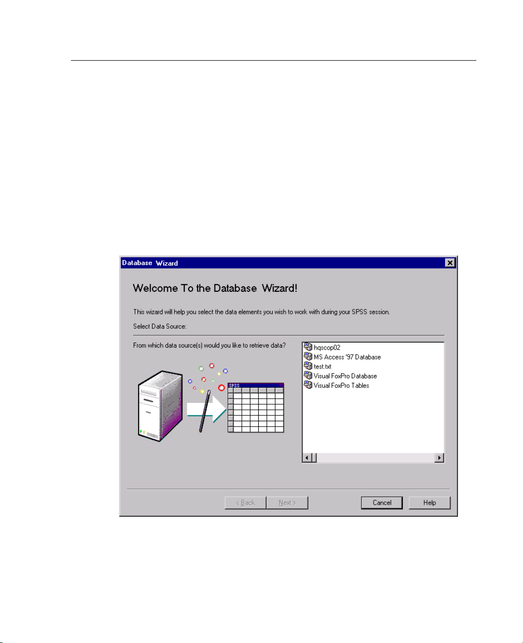
Use the first dialog box to select the type of data source to read into the software.
After you have chosen the file type, the Database Wizard may prompt you for the
path to you
If you do not have any data sources configured, or if you want to add a new data
source, click
version),
mode, see your system administrator.
r data file.
AddDataSource. In distributed analysis mode (available with the server
this button is not available. To add data sources in distributed analysis
Page 51
25
Data Files
Data sources. A data source consists of two essential pieces of information: the driver
that will be used to access the data and the location of the database that you want to
access. To s
pecify data sources, you must have the appropriate drivers installed. For
local analysis mode, you can install drivers from the CD-ROM for this product:
SPSS Data Access Pack. Installs drivers for a variety of database formats.
Available o
Microsoft
n the AutoPlay menu.
Data Access Pack.
Installs drivers for Microsoft products, including
Microsoft Access. To install the Microsoft Data Access Pack, double-click
Microsoft Data Access Pack in the Microsoft Data Access Pack folder on the
CD-ROM.
Figure 3-1
Database Wizard dialog box
Page 52
26
Chapter 3
Example. Let's say you have a Microsoft Access 7.0 database that c ontains data about
your employees and about the regions in which they work, and you want to import
that data. S
see the Select Database dialog box. Specify the path to your database and click OK.
elect the
MS Access 7.0 Database icon, and click Next to proceed. You will
Database Lo
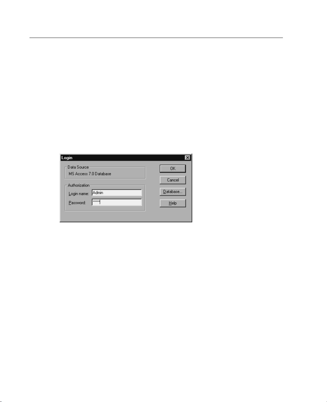
If your dat
one before it can open the data source.
Figure 3-2
Login dial
gin
abase requires a password, the Database Wizard will prompt you for
og box
Selecting Data Fields
The Select Data dialog box controls which tables and fields are read into the software.
se fields (columns) are read as variables.
Databa
If a table has any field(s) selected, all of its fields will be visible in the following
Database Wizard windows, but only those fields selected in this dialog box will be
ed as variables. This enables you to create table joins and to specify criteria
import
using fields that you are not importing.
Page 53
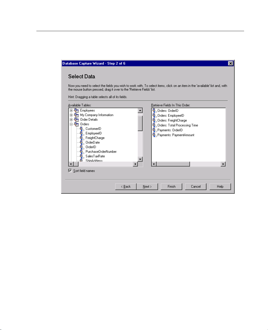
Figure 3-3
Select Data dialog box
27
Data Files
Displaying field na mes. To list the fields in a table, click the plus sign (+) to the left of
a table name. To hide the fields, click the minus sign (–) to the left of a table name.
To add a field. Double-click any field in the Available Tables list, or drag it to the
Retrieve Fields in This Order list. Fields can be reordered by dragging and dropping
them within the selected fields list.
To remove a field. Double-click any field in the Retrieve Fields in This Order list,
or drag it to the Available Tables list.
Sort field n ames. If selected, the Database Wizard will display your available fields
in alphabetical order.
Example. Assume that you want t o import from a database with two tables, Employees
and Regions. The Employees table contains information about your company's
employees, including the region they work in, their job category, and their annual
Page 54
28
Chapter 3
sales. Employees are each assigned a region code (REGION), while those who do
not have a home region get the special code of 0. The Regions table holds a large
amount of da
ta about the areas in which your company operates and prospective
markets.Itusesaregioncode(REGION) to identify the area and provides the average
per capita income for the area, among other things. To relate each employee's sales
to the aver
age income in the region, you would select the following fields from the
Employees table: ID, REGION,andSALES. Then, select the following fields from
the Regions table: REGION and AVGINC.Click
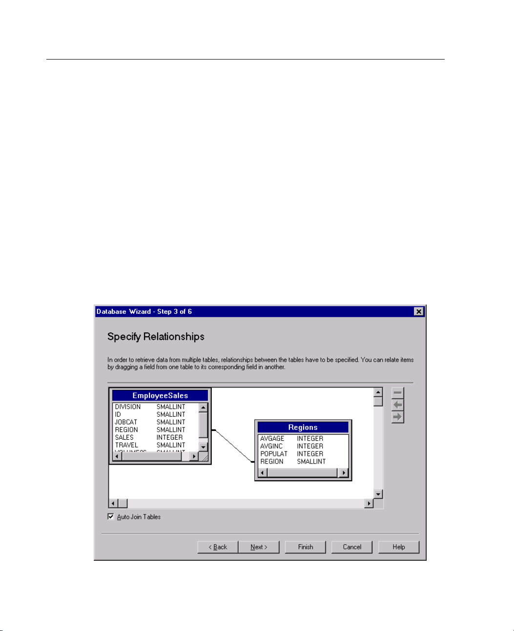
Creating a Relationship between Tables
The Specify Relationships dialog box allows you to define the relationships between
the tables. If fields from more than one table are selected, you must define at least
one join.
Figure 3-4
Specify Relationships dialog box
Next to proceed.
Page 55
29
Data Files
Establishing relationships. Tocreatearelationship,dragafieldfromanytableontothe
field to which you want to join it. The Database Wizard will draw a join line between
the two fiel
Auto Join Tables. Attempts to automatically join tablesbasedonprimary/foreignkeys
ds, indicating their relationship. These fields must be of the same data type.
or matching field names and data type.
Specifying
join types.
either inner joins, left outer joins, or right outer joins. To select the type of join,
click the join line between the fields, and the software will display the Relationship
Propertie
sdialogbox.
You can also use the icons in the upper right corner of the dialog box to choose
the type of join.
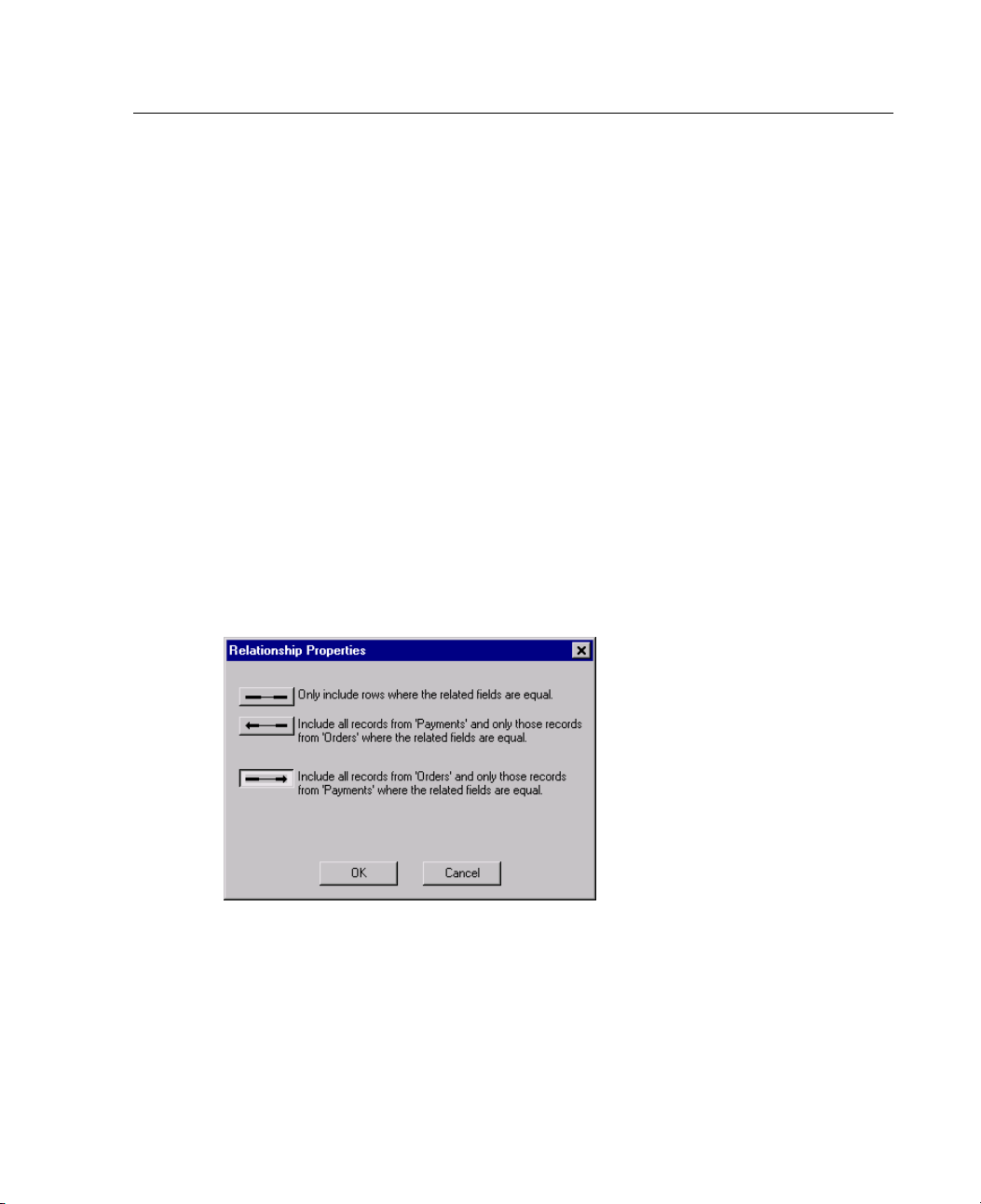
Relationship Properties
This dialog box allows you to specify which type of relationship joins your tables.
Figure 3-5
Relation
ship Properties dialog box
If outer joins are supported by your driver, you can specify
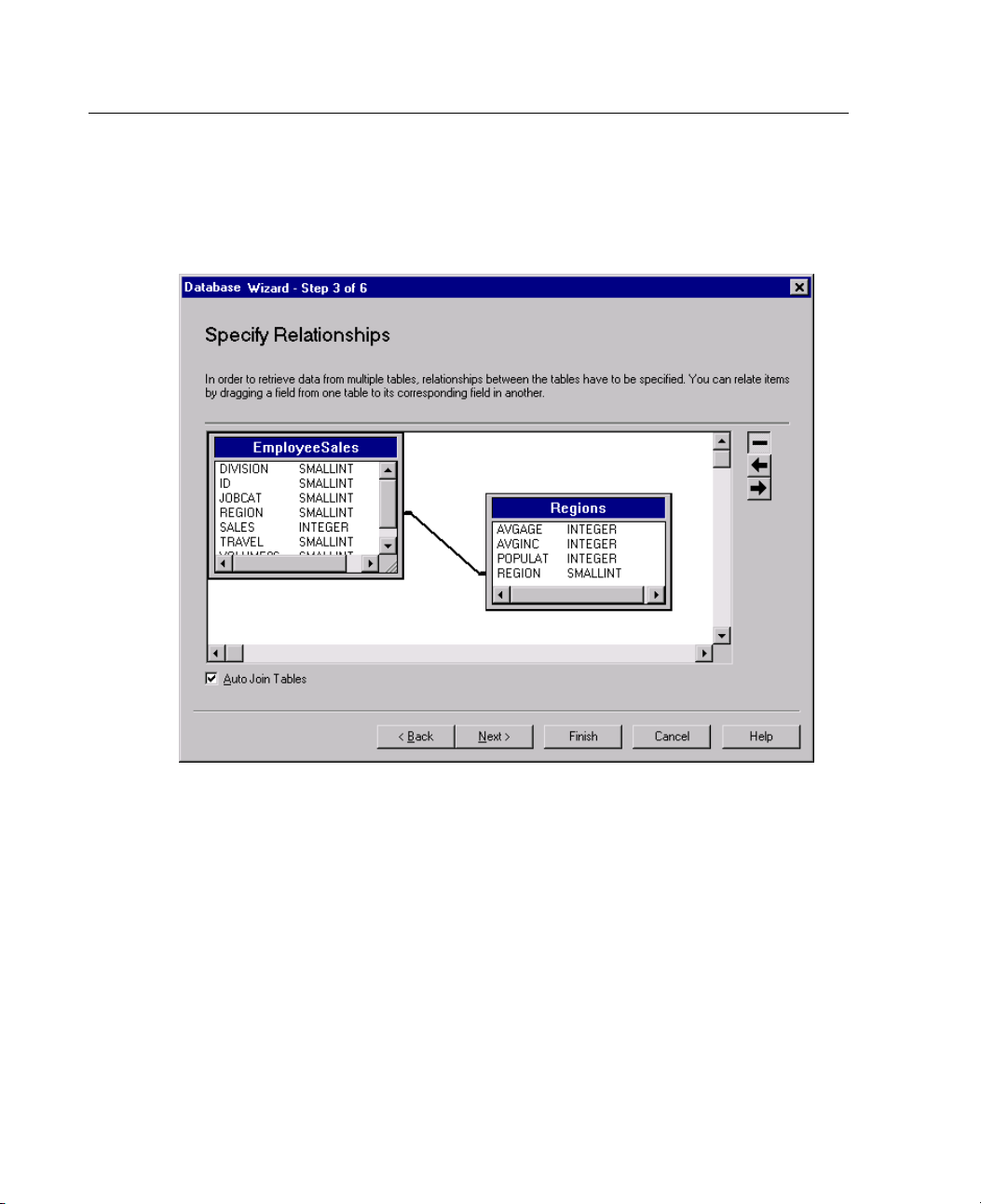
Inner joins. An inner join includes o nly rows where the related fields are equal.
Example. Continuing with our data, suppose that y ou want to import data only for
mployees who work in a fixed region and only for those regions in w hich your
those e
company operates. In this case, you would use an inner join, which would exclude
traveling employees and would filter out information about prospective regions in
you do not currently have a presence.
which
Page 56
30
Chapter 3
Completing this would give you a data set that contains the variables ID, REGION,
SALES95,andAVGINC foreachemployeewhoworkedinafixedregion.
Figure 3-6
Creating an inner join
Outer joins. A left outer join includes all records from the table on the left and only
those records from the table on the right in which the related fields are equal. In a
right outer join, this relationship is switched, so that the software imports all records
from the table on the right and only those records from the table on the left in which
the related fields are equal.
Example. Ifyouwantedtoimportdataonlyforthoseemployeeswhoworkedinfixed
regions (a subset of the Employees table) but needed information about all of the
regions, a right outer join would be appropriate. This results in a data set that contains
the variables ID, REGION, SALES95,andAVGINC for each employee who worked
in a fixed region, plus data on the remaining regions in which your company does
not currently operate.
Page 57
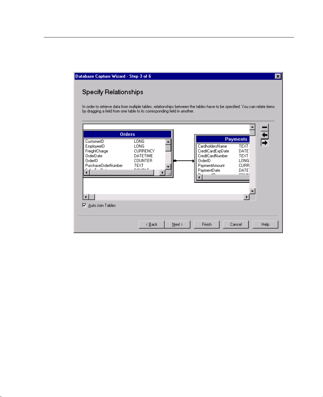
Figure 3-7
Creating a r ight outer join
31
Data Files
Limiting Retrieved Cases
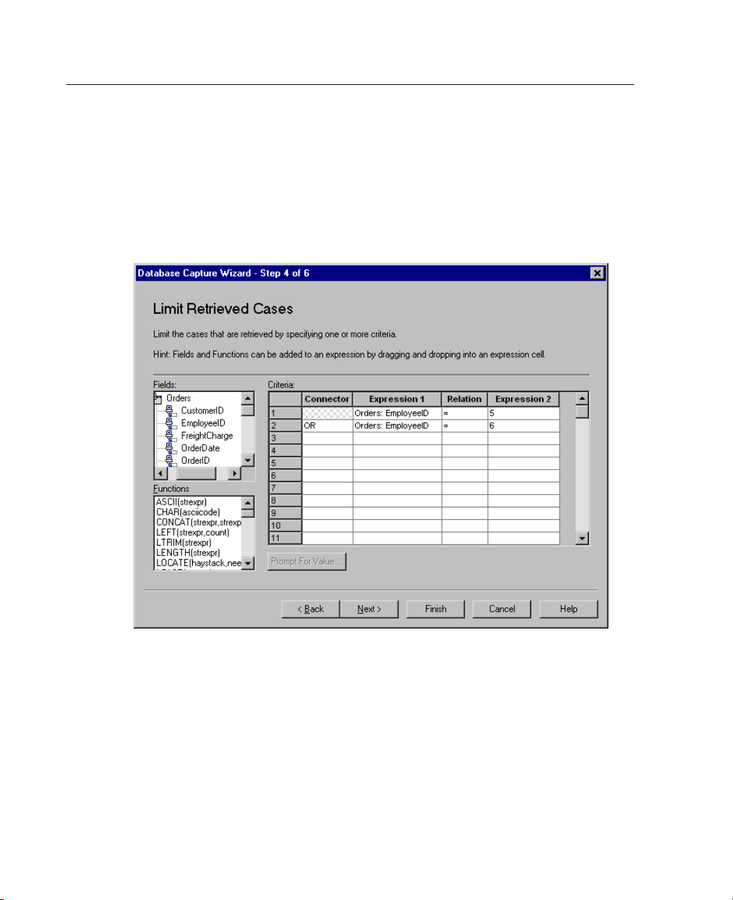
The Limit Retrieved Cases dialog box allows you t o specify the criteria to select
subsets of cases (rows). Limiting cases generally consists of filling the criteria grid
with one or more criteria. Criteria consist of two expressions and some relation
between them. They return a value of true, false,ormissing for each case.
If the result is true, the case is selected.
If the result is false or missing, the case is not selected.
Page 58
32
Chapter 3
Most criteria use one or more of the six relational operators (<, >, <=, >=,
=, and <>).
Expression
s can include field names, constants, arithmetic operators, numeric
and other functions, and logical variables. You can use fields that you do not
plan to import as variables.
Figure 3-8
Limit Retri
eved Cases dialog box
To build your criteria, you need at least two expressions and a relation to connect them.
E To build an expression, put your cursor in an Expression cell. You can type field
names, constants, arithmetic operators, numeric and other functions, and logical
variables. Other methods of putting a field into a criteria cell include double-clicking
the field in the Fields list, dragging the field from the Fields list, or selecting a field
from the drop-down menu that is available in any active Expression cell.
Page 59

Data Files
E
The two expressions are usually connected by a relational operator, such as = or >. To
choose the relation, put your cursor in the Relation cell and either type the operator
or select it
from the drop-down menu.
33
To modify ou
r earlier example to retrieve data only about employees who fit into
job categories 1 or 3, create two criteria in the criteria grid, and prefix the second
criteria with the connector
Criteria 1:
'EmployeeSales'.'JOBCAT' = 1
OR.
Criteria 2: 'EmployeeSales'.'JOBCAT' = 3
Functions. A selection of built-in arithmetic, logical, string, date, and time SQL
functions are provided. You can select a function from the list and drag it into
the expres
sion, or you can enter any valid SQL function. See your database
documentation for valid SQL functions.
Use Rando m Sampling. Selects a random sample of cases from the data source.
For large d
ata sources, you may want to limit the number of cases to a small,
representative sample. This can significantly reduce the time that it takes to run
procedures. Native random sampling, if available for the data source, is faster than
SPSS rand
om sampling, since SPSS random sampling must still read the entire
data source to extract a random sample.
Approximately. Generates a random sample of approximately the specified
percent
age of cases. Since this routine makes an independent pseudo-random
decision for each case, the percentage of cases selected can only approximate
the specified percentage. The more cases there are in the data file, the closer the
percent
Exactl
age of cases selected is to the specified percentage.
y.
Selects a random sample of the specified number of cases from the
specified total number of cases. If the total number of cases specified exceeds
the total number of cases in the data file, the sample will contain proportionally
fewer c
ases than the requested number.
Prompt for Value. You can embed a prompt in your query to create a parameter query.
When users run the query, they will be asked to enter information specified here. You
might w
ant to do this if you need to see different views of the same data. For example,
you may want to run the same query to see sales figures for different fiscal quarters.
Place your cursor in any Expression cell, and click
Prompt for Value to create a prompt.
Page 60
34
Chapter 3
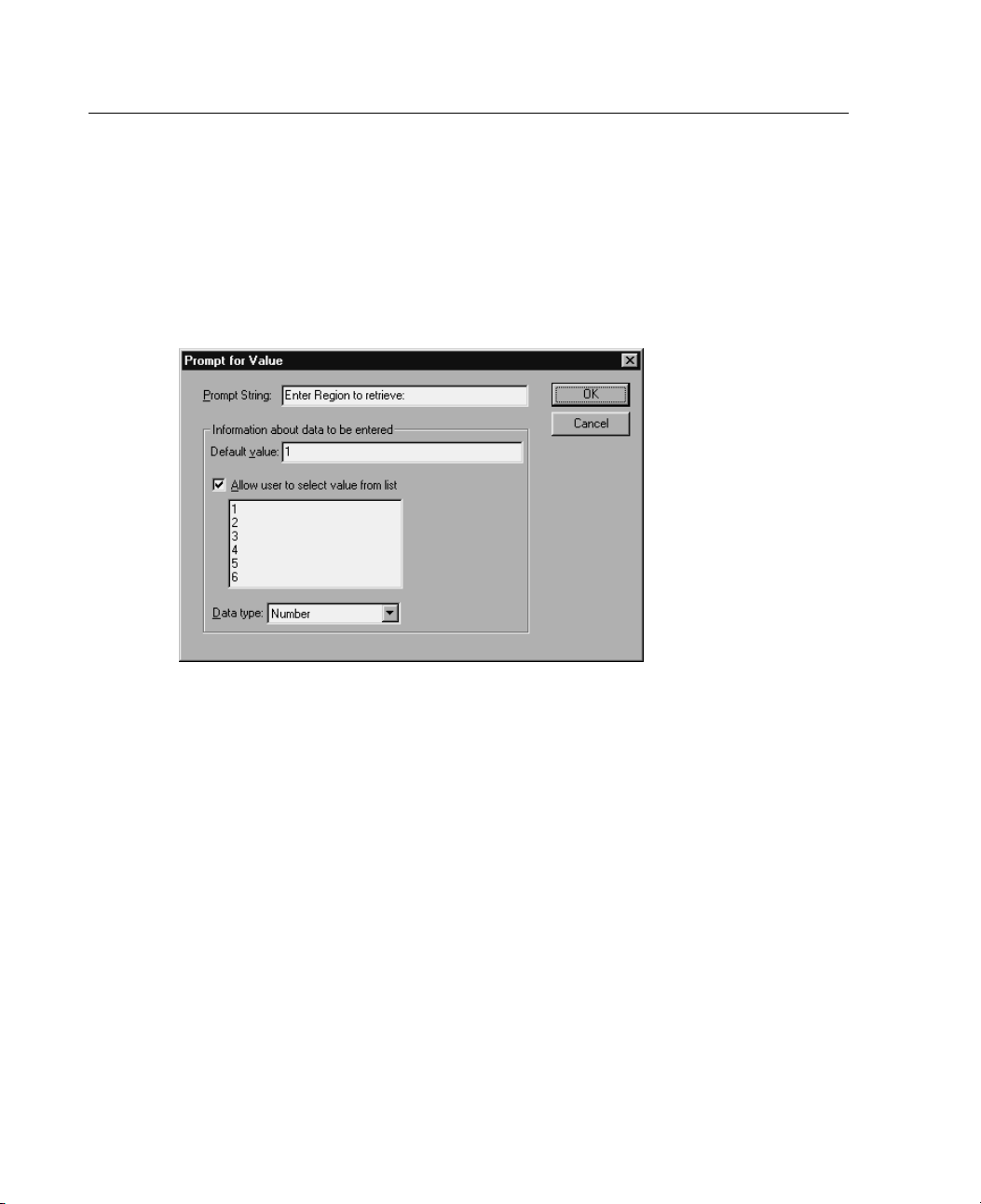
Creating a Pa
Use the Prom
from users each time someone runs your query. It is useful if you want to query the
same data source using different criteria.
Figure 3-9
Prompt for Value dialog box
To build a prompt, you need to enter a prompt string and a default value. The prompt
s displayed each time a user runs your query. It should specify the kind of
string i
information to enter, and, if the user is not selecting from a list, it should give hints
about how the input should be formatted. Forexample,“EnteraQuarter(Q1,Q2,
)”.
Q3, ...
rameter Query
pt for Value dialog box to create a dialog box that solicits information
Allow user to select valu e from list. If this is selected, you can limit the user to the
values you place here, which are separated by carriage returns.
pe.
Data ty
Specify the data type here, either number, string,ordate.
Page 61
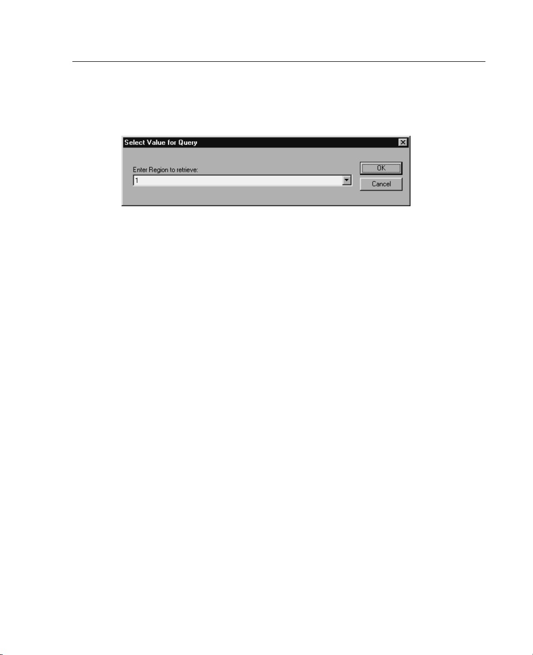
The final result looks like this:
35
Data Files
Figure 3-10
User-define
dpromptdialogbox
Defining Variables (Database Wizard)
Variable names and labels. The complete database field (column) name is used as the
variable label. Unless you modify the variable name, the Database Wizard assigns
variable names to each column from the database in one of two ways:
If the name of the database field forms a valid, unique variable name, it is used
as the variable name.
If the name of the database field does not form a valid, unique variable name,
the software creates a unique name.
Click any cell to edit the variable name.
Converting strings to numeric values. Check the Value Labels box for a string variable if
you want to automatically convert it to a numeric variable. String values are converted
to consecutive integer values based on alphabetic order of the original values. The
original values are retained as value labels for the new variables.
Page 62
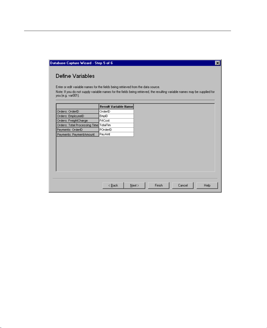
36
Chapter 3
Figure 3-11
Define Variables dialog box
Results
The Results dialog box displays the SQL Select statement for your query.
You can edit the SQL Select statement before you run the query, but if you
click the
Back button to make changes in previous steps, the changes to the
Select statement will be lost.
You can save the query for future use with Save query to a file.
Select Paste it into the syntax editor for further modification to paste complete GET
syntax into a syntax window. Copying and pasting the Select statement
DA TA
from the Results window will not paste the necessary command syntax.
Page 63
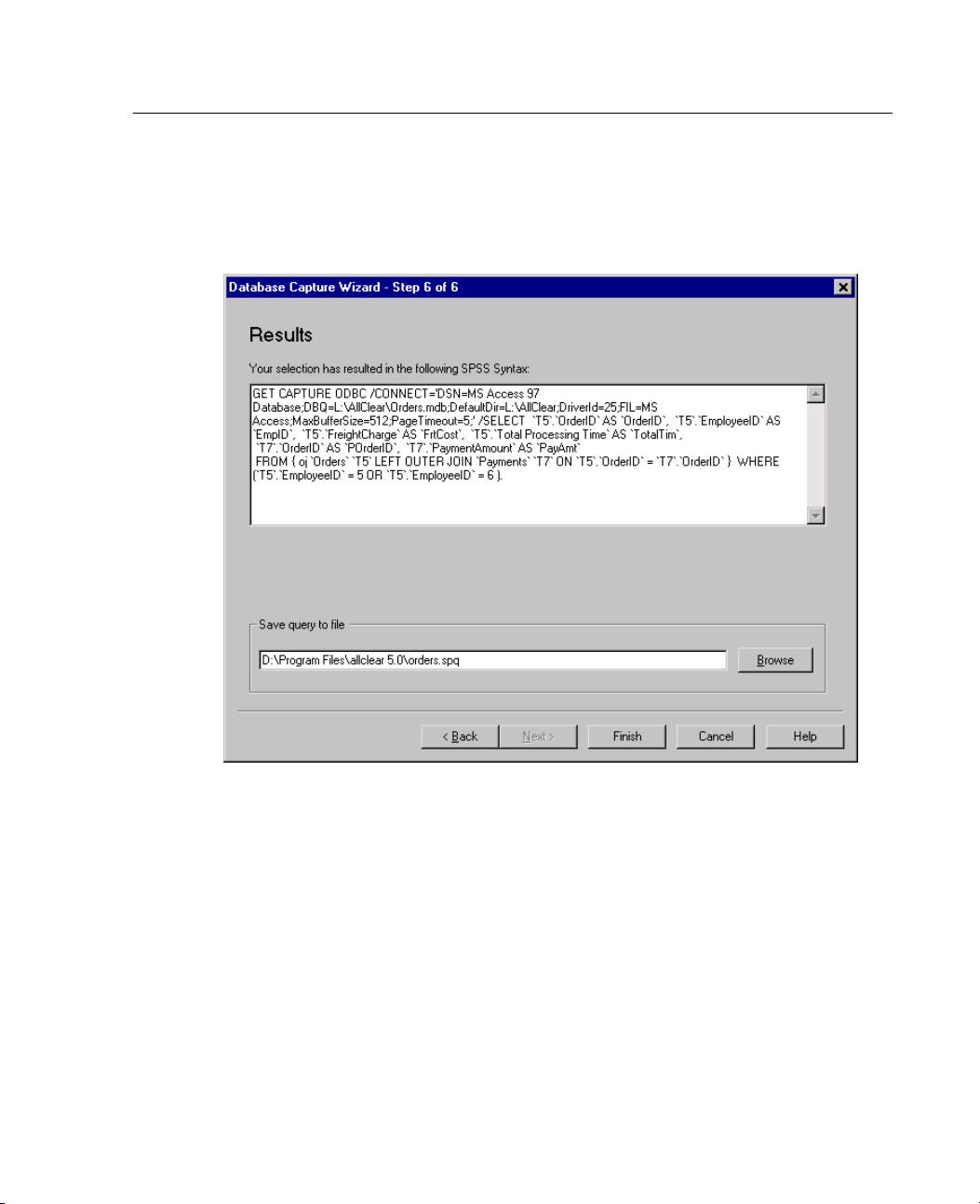
37
Data Files
Cache data locally. A data cache is complete copy of the data file, stored in temporary
disk space. Caching the data file can improve performance.
Figure 3-12
Results dialog box
Text Wizard
The Text Wizard can read text data files formatted in a variety of ways:
Tab-delimited files
Space-delimited files
Comma-delimited files
Fixed-field format files
For delimited files, you can also specify other characters as delimiters between
values, and you can specify multiple delimiters.
Page 64
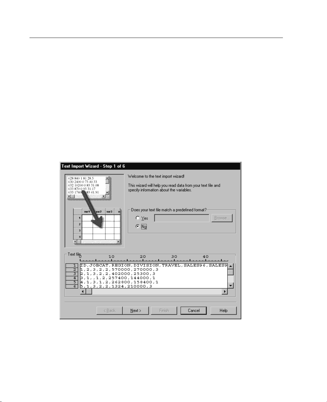
38
Chapter 3
To Read Text Data Files
E From the menus choose:
File
Read Text Data
Select the text file in the Open dialog box.
E
E Follow the steps in the Text Wizard to define how to read the data file.
Text Wizard Step 1
Figure 3-13
Tex t W i z ar d
Step 1
The text file is displayed in a preview window. You can apply a predefined format
(previously saved from the Text Wizard) or follow the steps in the Text Wizard
cify how the data should be read.
to spe
Page 65
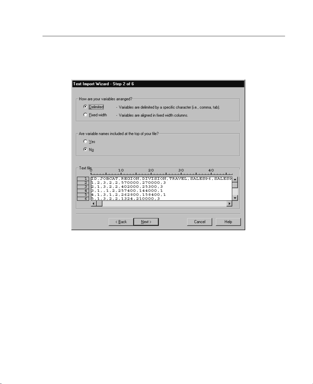
Text Wizard Step 2
39
Data Files
Figure 3-14
Tex t W i z ar d S
tep 2
This step provides information about variables. A variable is similar to a field in a
database. For example, each item in a questionnaire is a variable.
e your variables arra nge d?
How ar
To read your data properly, the Text Wizard needs to
know how to determine where the data value for one variable ends and the data value
for the next variable begins. The arrangement of variables defines the method used to
rentiate one variable from the next.
diffe
mited.
Deli
Spaces, commas, tabs, or other characters are used to separate
variables. The variables are recorded in the same order for each case but not
necessarily in the same column locations.
Fixed width. Each variable is recorded in the same column location on the same
rd (line) for each case in the data file. No delimiter is required between
reco
variables. In fact, in many text data files generated by computer programs, data
Page 66
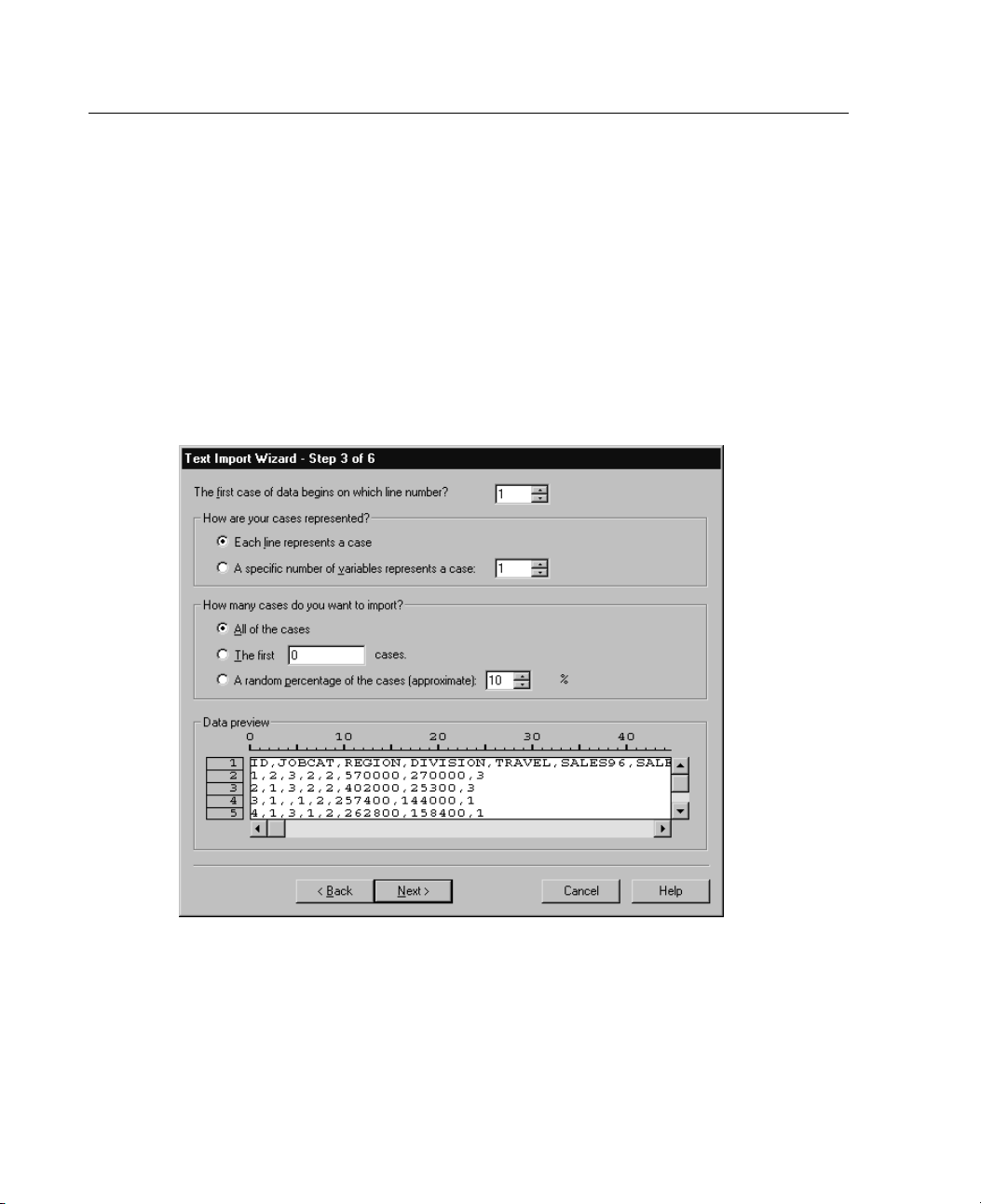
40
Chapter 3
values may appear to run together without even spaces separating them. The
column loca
Are variable names included at the top of your file? If the first row of the data file
tion determines which variable is being read.
contains descriptive labels for each variable, you can use these labels as variable
names. Valu
es that don't conform to variable naming rules are converted to valid
variable names.
Text Wizar
Figure 3-15
Text Wi zard Step 3 for delimited files
d Step 3: Delimited Files
step provides information about cases. A case is similar to a record in a database.
This
For example, each respondent to a questionnaire is a case.
Page 67

Data Files
The first case of data begins on which line number? Indicates the first line of the data
file that contains data values. If the top line(s) of the data file contain descriptive
labels or ot
How are your cases represented? Controls how the Text Wizard determines where
her text that does not represent data values, this will not be line 1.
each case ends and the next one begins.
Each line represents a case. Each line contains only one case. It is fairly common
for each case to be contained on a single line (row), even though this can be a
very long l
ine for data files with a large number of variables. If not all lines
contain the same number of data values, the number of variables for each case is
determined by the line with the greatest number of data values. Cases with fewer
data value
A specifi
s are assigned missing values for the additional variables.
c number of variables represents a case.
The specified number of variables
for each case tells the Text Wizard where to stop reading one case and start
reading the next. Multiple cases can be contained on the same line, and cases can
start in t
he middle of one line and be continued on the next line. The T ext Wizard
determines the end of each case based on the number o f values read, regardless
of the number of lines. Each case must contain data values (or missing values
ed by delimiters) for all variables, or the data file will be read incorrectly.
indicat
41
How many cases do you want to import? You can import all cases in the data file, the
first n cases (n is a number you specify), or a random sample of a specified percentage.
Since th
e random sampling routine makes an independent pseudo-random decision
for each case, the percentage of cases selected can only approximate the specified
percentage. The more cases there are in the data file, the closer the percentage of
elected is to the specified percentage.
cases s
Page 68
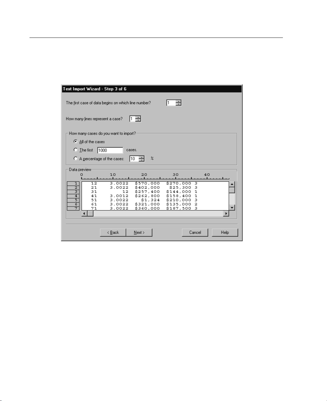
42
Chapter 3
Text Wizard Step 3: Fixed-Width Files
Figure 3-16
Tex t W iz a r d S
tep 3 for fixed-width files
This step provides information about cases. A case is similar to a record in a database.
For example, each respondent to questionnaire is a case.
The first case of data begins on which line number? Indicates the first line of the data
file that contains data values. If the top line(s) of the data file contain descriptive
labels or other text that does not represent data values, this will not be line 1.
How many lines re pre sent a case? Controls how the Text Wizard determines where
each case ends and the next one begins. Each variable is defined by its line number
within the case and its column location. You need to specify the number of lines
for each case to read the data correctly.
Page 69
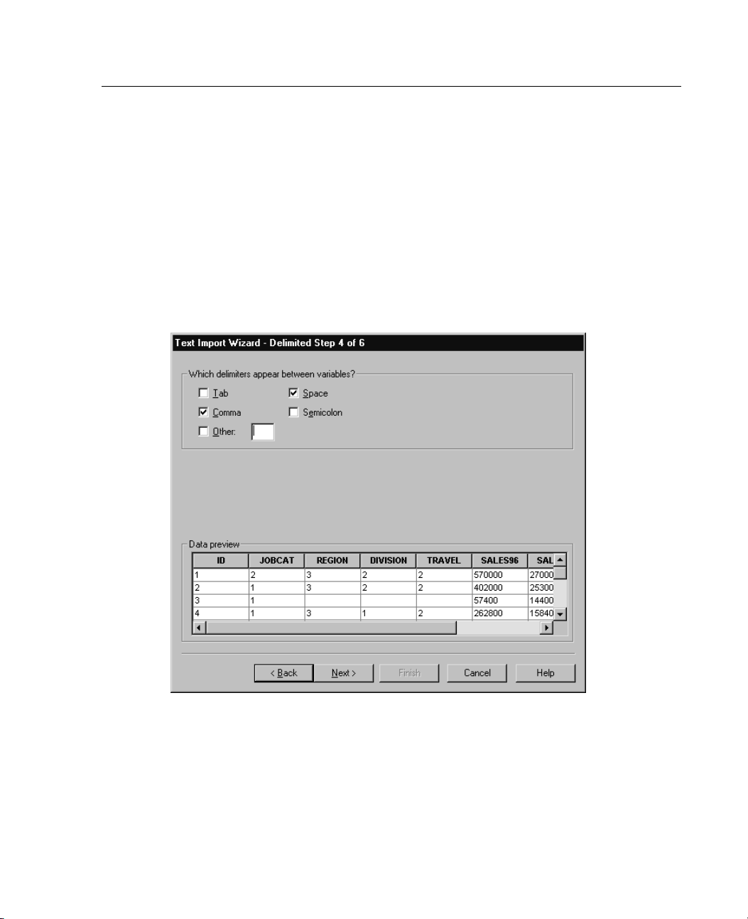
How many cases do you want to import? You can import all cases in the data file, the
first n cases (n is a number you specify), or a random sample of a specified percentage.
Since the ra
ndom sampling routine makes an independent pseudo-random decision
for each case, the percentage of cases selected can only approximate the specified
percentage. The more cases there are in the data file, the closer the percentage of
cases sele
cted is to the specified percentage.
Text Wizard Step 4: Delimited Files
Figure 3-17
Text Wi zard Step 4 for delimited files
43
Data Files
This step displays the Text Wizard's best guess on how to read the data file and allows
o modify how the Text Wizard will read variables from the data file.
you t
Page 70
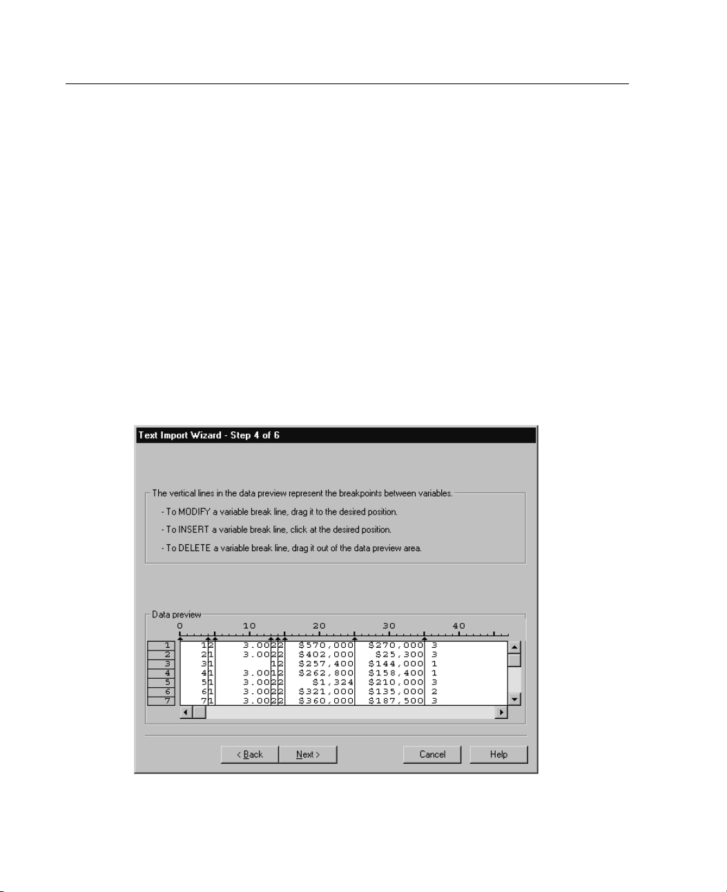
44
Chapter 3
Which delimiters appear between variables? Indicates the characters or symbols that
separate data values. You can select any combination of spaces, commas, semicolons,
tabs, or oth
er characters. Multiple, consecutive delimiters without intervening data
values are treated as missing values.
What is the text qualifier? Characters used to enclose values that contain delimiter
characters
. For example, if a comma is the delimiter, values that contain commas
will be read incorrectly unless there is a text qualifier enclosing the value, preventing
the commas in the value from being interpreted as delimiters between values.
CSV-forma
t data files exported from Excel use a double quotation mark (“) as a text
qualifier. The text qualifier appears at both the beginning and the end of the value,
enclosing the entire value.
Text Wizard Step 4: Fixed-Width Files
Figure 3-
Tex t W iz a
18
rd Step 4 for fixed-width files
Page 71
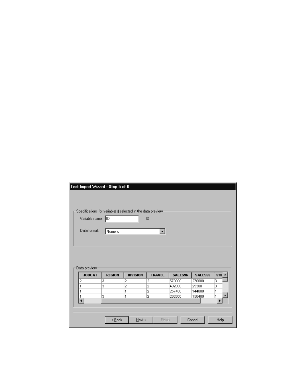
This step displays the Text Wizard's best guess on how to read the data file and allows
you to modify how the Text Wizard w ill read variables from the data file. Vertical
lines in the
variable begins in the file.
Insert, move, and delete variable break lines as necessary to separate variables. If
multiple li
nes are used for each case, select each line from the drop-down list and
modify the variable break lines as necessary.
Note: For computer-generated data files that produce a continuous stream of data
values wit
h no intervening spaces or other distinguishing characteristics, it may
be difficult to determine where each variable begins. Such data files usually rely
on a data definition file or some other written description that specifies the line
and column
Text Wizard Step 5
Figure 3-19
Tex t W i z ar d St e p 5
45
Data Files
preview window indicate where the Text Wizard currently thinks each
location for each variable.
Page 72

46
Chapter 3
This steps controls the variable name and the data format that the Text Wizard will
use to read each variable and which variables will be included in the final data file.
Variable na
me.
variable names. If you read variable names from the data file, the Text Wizard will
automatically modify variable names that don't conform to variable naming rules.
Select a var
Data format. Select a variable in the preview window and then select a format from the
iable in the preview window and then enter a variable name.
drop-down list. Shift-click to select multiple contiguous variables or Ctrl-click to
select mul
tiple noncontiguous variables.
Text Wizard Formatting Options
Formatting options for reading variables with the Text Wizard include:
Do not import. Omit the selected variable(s) from the imported data file.
You can overwrite the d efault variable names with your own
Numeric. V
alid values include numbers, a leading plus or minus sign, and a decimal
indicator.
String. Valid values include virtually any keyboard characters and embedded blanks.
For delim
ited files, you can specify the number of characters in the value, up to a
maximum of 255. By default, the Text Wizard sets the number of characters to the
longest string value encountered for the selected variable(s). For fixed-width files,
the numbe
r of characters in string values is defined by the placement of variable
break lines in step 4.
Date/Time. Valid values include dates of the general format dd-mm-yyyy, mm/dd/yyyy,
dd.mm.y
yyy, yyyy/mm/dd, hh:mm:ss, and a variety of other date and time formats.
Months can be represented in digits, Roman numerals, or three-letter abbreviations,
or they can be fully spelled out. Select a date format from the list.
Valid values are numbers with an optional leading dollar sign and optional
Dollar.
commas as thousands separators.
Comma. Valid values include numbers that use a period as a decimal indicator and
commas
Dot. Valid values include numbers that use a comma as a decimal indicator and
as thousands separators.
periods as thousands separators.
Page 73
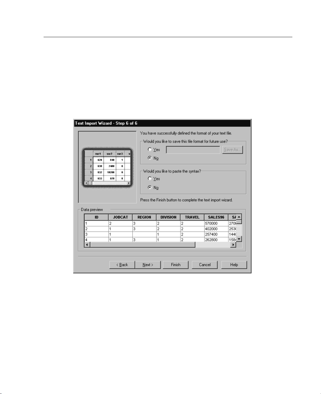
Note: Values that contain invalid characters for the selected format will be treated
as missing. Values that contain any of the specified delimiters will be treated as
multiple va
Text Wizard Step 6
Figure 3-20
Tex t W i z ar d St e p 6
47
Data Files
lues.
This is the final step of the Text Wizard. You can save your specifications in a file for
en importing similar text data files. You can also paste the syntax generated
use wh
by the Text Wizard into a syntax window. You can then customize and/or save the
syntax for use in other sessions or in production jobs.
Cache data locally. A data cache is complete copy of the data file, stored in temporary
space. Caching the data file can improve performance.
disk
Page 74

48
Chapter 3
File Informa
Adatafilec
information, including:
Variable names
Variable formats
Descriptive variable and value labels
This information is stored in the dictionary portion of the data file. The Data Editor
provides on
complete dictionary information for the working data file or any other data file.
To Obtain Da
E From the me
E
E For other data files, choose: External File, and then select the data file.
ta File Information
File
Display Data File Information
For the currently open data file, choose Working File.
The data file information is displayed in the Viewer.
tion
ontains much more than raw data. It also contains any variable definition
e way to view the variable definition information. You can also display
nus in the Data Editor window choose:
Saving Data Files
Any changes that you make in a data file last only for the duration of the current
session—unless you explicitly save the changes.
To Save Modified Data Files
E Make the Data Editor the active window (click anywhere in the window to make it
active).
E From the menus choose:
File
Save
Page 75

The modified data file is saved, overwriting the previous version of the file.
49
Data Files
Saving Data
You can save
format depends on the version of Excel that will be used to open the data. The Excel
application cannot open an Excel file from a newer version of the application. For
example, E
can easily read an Excel 5.0 document.
There a re a few limitations to the Excel file format that don't exist in SPSS. These
limitatio
Variable
in exported Excel files.
WhenexportingtoExcel97andlater,anoptionisprovidedtoincludevalue
labels instead of values.
Because all Excel files are limited to 256 columns of data, only the first 256
variables
Excel 4.0
Excel 97–2000 files allow 65,536 records. If your data exceed these limits, a
warning message is displayed and the data are truncated to the maximum size
allowed b
Variable Types
Files in Excel Format
your data in one of three Microsoft Excel file formats. The choice of
xcel 5.0 cannot open an Excel 2000 document. However, Excel 2000
ns include:
information, such as missing values and variable labels, is not included
are included in the exported file.
and Excel 5.0/95 files are limited to 16,384 records, or rows of data.
yExcel.
The following table shows the variable type matching between the original data in
SPSS and t
SPSS Variable Type Excel Data Format
Numeric 0.00; #,##0.00;...
Comma 0.00; #,##0.00;...
Dollar
Date d-mmm-yyyy
Time hh:mm:ss
String General
he exported data in Excel.
$#,##0_);...
Page 76

50
Chapter 3
Saving Data F
Special han
These cases include:
Certain characters that are allowed in SPSS variable names are not valid in SAS,
such as @, #,
when the data are exported.
SPSS variable labels containing more than 40 characters are truncated when
exported to a SAS v6 file.
Where they exist, SPSS variable labels are mapped to the SAS variable labels.
If no varia
the SAS variable label.
SAS allows only one value for system-missing, whereas SPSS allows numerous
system-missing values. As a result, all system-missing values in SPSS are
mapped to a
Save Value Labels
You have the option of saving the values and value labels associated with your data
file to a S
are exported, the generated syntax file contains:
iles in SAS Format
dling is given to various aspects of your data when saved as a SAS file.
and $. These illegal characters are replaced with an underscore
ble label exists in the SPSS data, the variable name is mapped to
single system-missing value in the SAS file.
AS syntax file. For example, when the value labels for the cars.sav data file
libname library 'd:\spss\' ;
proc format library = library ;
value ORIGIN /* Country of Origin */
1 = 'America
2 = 'European'
3 = 'Japanese' ;
value CYLIND
3 = '3 Cylinders'
4 = '4 Cylinders'
5 = '5 Cylinders
6 = '6 Cylinders'
n'
ER /* Number of Cylinders */
'
Page 77

51
Data Files
8 = '8 Cylinde
value FILTER__ /* cylrec=1|cylrec = 2 (FILTER) */
0 = 'Not Selected'
1 = 'Selected' ;
proc datasets l
modify cars;
format ORIGIN ORIGIN.;
format CYLINDER C
format FILTER__ FILTER__.;
quit;
This feature is not
rs' ;
ibrary = library ;
YLINDER.;
supported for the SAS transport file.
Variable Types
The following table shows the variable type matching between the original data
in SPSS and the exp
SPSS Variable Type SAS Variable Type SAS Data Format
Numeric Numeric 12
Comma N umeric 12
Dot Numeric 12
Scientific Notation Numeric 12
Date Numeric (Date) for example,
Date (Time) Numeric Time18
Dollar Numeric 12
Custom Currency Numeric 12
String Character
orted data in SAS:
MMDDYY10,...
$8
Page 78

52
Chapter 3
Saving Data F
E Make the Da
active).
E From the menus choose:
File
Save As...
Select a file type from the drop-down list.
E
E Enter a filename for the new data file.
To write variable names to the first row of a spreadsheet or tab-delimited data file:
E Click Write variable names to spreadsheet in the Save Data A s dialog box.
To save valu
E Click Save
dialog box.
To save valu
E Click Save
iles in Other Formats
ta Editor the active window (click anywhere in the window to make it
e labels instead of data values in Excel 97 format:
value labels where defined instead of data values
e labels to a SAS syntax file (active only when a SAS file type is selected):
value labels into a .sas file
in the Save Data As dialog box.
intheSaveDataAs
Saving Data: Data File Types
You can save data in the following formats:
v).
SPSS (*.sa
versions of the software prior to version 7.5. When using data files with variable
names longer than eight bytes in SPSS 10.x or 11.x, unique, eight byte versions of
variable n
release 12.0 or later. In r eleases prior to SPSS 10, the original long variable names are
lost if you save the data file.
SPSS 7.0 (
can be read by SPSS 7.0 and earlier versions of SPSS for Windows but do not include
defined multiple response sets or Data Entry for Windows information.
SPSS format. Data files saved in SPSS format cannot be read by
ames are used—but the original variable names are preserved for use in
*.sav).
SPSS 7.0 for Windows format. Data files saved in SPSS 7.0 format
Page 79

Data Files
SPSS/PC+ (*.sys). SPSS/PC+ format. If the data file contains more than 500
variables, only the first 500 will be saved. For variables with more than one defined
user-missi
ng value, additional user-missing values will be recoded into the first
defined user-missing value.
SPSS Portable (*.por). SPSS portable format that can be read by other versions of
SPSS and ver
sions on other operating systems (for example, Macintosh or UNIX).
Variable names are limited to eight bytes and are automatically converted to unique
eight byte names if necessary.
53
Tab-delim
Fixed ASCII (*.dat). ASCII text file in fixed format, using the default write formats for
ited (*.dat).
ASCII text files with values separated by tabs.
all variables. There are no tabs or spaces between variable fields.
*.xls).
Excel 2.1(
Microsoft Excel 2.1 spreadsheet file. The maximum number of
variables is 256, and the maximum number of rows is 16,384.
Excel 97 and later (*.xls). Microsoft Excel 97/2000/XP spreadsheet file. The maximum
number of v
1-2-3 Release 3.0 (*.wk3). Lotus 1-2-3 spreadsheet file, release 3.0. The maximum
ariables is 256, and the maximum number of rows is 65,536.
number of variables that you can save is 256.
1-2-3 Rel
ease 2.0 (*.wk1).
Lotus 1-2-3 spreadsheet file, release 2.0. The maximum
number of variables that you can save is 256.
1-2-3 Release 1.0 (*.wks). Lotus 1-2-3 spreadsheet file, release 1A. The maximum
number of
SYLK (*.slk). Symbolic link format for Microsoft Excel and Multiplan spreadsheet
variablesthatyoucansaveis256.
files. The maximum number of variables that you can save is 256.
*.dbf).
dBASE IV (
dBASE III (*.d bf). dBASE III format.
dBASE II (*.dbf). dBASE II format.
dBASE IV format.
SAS v6 for
SAS v6 for UNIX (*.ssd01). SAS v6 file format for UNIX (Sun, HP, IBM).
SAS v6 for Alpha/OSF (*.ssd04). SAS v6 file format for Alpha/OSF (DEC UNIX).
Windows (*.sd2).
SAS v6 file format for Windows/OS2.
Page 80
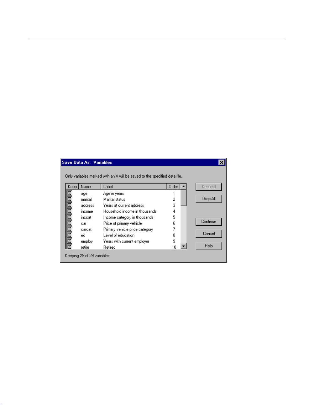
54
Chapter 3
SAS v7+ Windows short extension (*.sd7). SAS version 7-8 for Windows short
filename format.
SAS v7+ Wind
ows long extension (*.sas7bdat).
filename format.
SAS v7+ for UNIX (*.ssd01). SAS v8 for UNIX.
SAS Transpo
rt (*.xpt).
SAS transport file.
Saving Subsets of Variables
Figure 3-21
Save Data As Variables dialog box
SAS version 7-8 for Windows long
a saved as an SPSS data file, the Save Data As Variables dialog box allows you
For dat
to select the variables that you want to be saved in the new data file. By default, all
variables will be saved. Deselect the variables that you don't want to save, or click
and then select the variables that you want to save.
l
Drop Al
ToSaveaSubsetofVariables
E Make the Data Editor the active window (click anywhere in the window to make it
e).
activ
Page 81

E
From the menus choose:
File
Save As...
Select SPSS (*.sav) from the list of file types.
E
E Click Variables.
E Select the variables that you want to save.
Saving File Options
For spreadsheet and tab-delimited files, you can write variable names to the first
row of the file.
Protecting Original Data
To prevent the accidental modification/deletion of your original data, you can mark
the file as read-only.
55
Data Files
E From the Data Editor menus choose:
File
Mark File R
If you make
ead Only
subsequent modifications to the data and then try to save the data file, you
can save the data only with a different filename; so the original data are not affected.
You can change the file permissions back to read/write by selecting
Read Write
from the File menu.
Virtual Active File
The virtual active file enables you to work with large data files without requiring
equally l
charting procedures, the original data source is reread each time you run a different
procedure. Procedures that modify the data require a certain amount of temporary
disk spac
space for at least one entire copy of the data file.
arge (or larger) amounts of temporary disk space. For most analysis and
e to keep track of the changes, and some actions always require enough disk
Mark File
Page 82
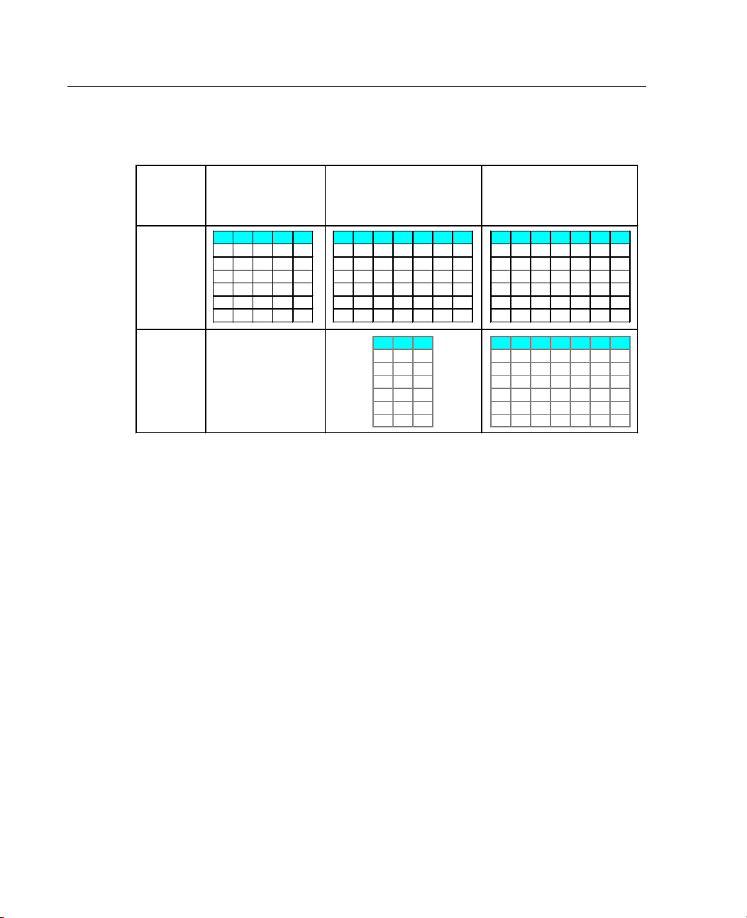
56
Chapter 3
Figure 3-22
Temporary disk space requirements
Action
Virtual
Active
File
GET FILE = 'v1-5.sav'. REGR ESSION … or
FREQUENCIES… /SAVE ZPRED.
v1 v2 v3 v4 v5 v1 v2 v3 v4 v5 v6 zpre v1 v2 v3 v4 v5 v6 zpre
11 12 13 14 15 11 12 13 14 15 16 1 11 12 13 14 15 16 1
21 22 23 24 25 21 22 23 24 25 26 2 21 22 23 24 25 26 2
31 32 33 34 35 31 32 33 34 35 36 3 31 32 33 34 35 36 3
41 42 43 44 45 41 42 43 44 45 46 4 41 42 43 44 45 46 4
51 52 53 54 55 51 52 53 54 55 56 5 51 52 53 54 55 56 5
61 62 63 64 65 61 62 63 64 65 66 6 61 62 63 64 65 66 6
COMPUTE v6 = …
RECODE v4…
SORT CASES BY…
CACHE
Data
Stored
in
Tem po rary
Disk
Space
Actions
that don't require any temporary disk space include:
Readin
Mergin
Readin
Mergin
Running
Actions
that create one or more columns of data in temporary disk space include:
Computi
Recodin
Running
None
g SPSS data files
g two or more SPSS data files
g database tables with the Database Wizard
g an SPSS data file with a database table
procedures that read data (for example, Frequencies, Crosstabs, Explore)
ng new variables
gexistingvariables
procedures that create or modify variables (for example, saving
v4 v6 zpre v1 v2 v3 v4 v5 v6 zpre
1416 1 111213141516 1
2426 2 212223242526 2
3436 3 313233343536 3
4446 4 414243444546 4
5456 5 515253545556 5
6466 6 616263646566 6
predicted values in Linear Regression)
Actions that create an entire copy of the da ta file in temporary disk space include:
Reading Excel files
Running procedures that sort data (for example, Sort Cases, Split File)
Reading data with GET TRANSLATE or DAT A LIST commands
Page 83

Data Files
Using the Cache Data facility or the CACHE command
Launching other applications from SPSS that read the data file (for example,
GET
DA TA
DecisionTime)
command provides functionality comparable to DA TA LIST,
AnswerTree,
Note:The
without c reating an entire copy of the data file in temporary disk space. The SPLIT
command in command syntax does not sort the data file and therefore does not
FILE
create a cop
y of the data file. This command, however, requires sorted data for
proper operation, and the dialog box interface for this procedure will automatically
sort the data file, resulting in a complete copy of the data file. (Command syntax is
not availa
ble with the Student Version.)
57
Actions th
Reading d
Reading t
The Databa
at create an entire copy of the data file by default
atabases with the Database Wizard
ext files with the Text Wizard
se Wizard and the Text Wizard provide an optional setting to automatically
cache the data. By default, this option is selected. You can turn it off by deselecting
Cache data locally.
Creating a Data Cache
Although the virtual active file can vastly reduce the amount of temporary disk space
required, the absence of a temporary copy of the “active” file means that the original
data sou
external source, creating a temporary copy of the data may improve performance. For
example, for data tables read from a database source, the SQL query that reads the
informa
needs to read the data. Since virtually all statistical analysis procedures and charting
procedures need to read the data, the SQL query is reexecuted for each procedure
you run
large number of procedures.
your lo
improve processing time by creating a data cache of the active file. The data cache is
a temporary copy of the complete data.
rce has to be reread for each procedure. For large data files read from an
tion from the database must be reexecuted for any command or procedure that
, which can result in a significant increase in processing time if you run a
If you have sufficient disk space on the computer performing the analysis (either
cal computer or a remote server), you can eliminate multiple SQL queries and
:
Page 84

58
Chapter 3
Note: By default, the Database Wizard automatically creates a data cache, but if you
use the GET FILE command in command syntax to read a database, a data cache is not
automatica
To Create a Data Cache
E From the menus choose:
File
Cache Data...
Click OK or Cache Now.
E
OK creates a data cache the next time the program reads the data (for example, the
next time y
doesn't require an extra data pass.
shouldn't be necessary under most circumstances. Cache Now is useful primarily
for two rea
Adatasou
session, open a different data source, or cache the data.
For large data sources, scrolling through the contents of the Data view in the Data
Editor will be much faster if you cache the data.
lly created. (Command syntax is not available with the Student Version.)
ou run a statistical procedure), which is usually what you want since it
Cache Now creates a data cache immediately,which
sons:
rce is “locked” and can't be updated by anyone until you end your
To Cache Data Automatically
You can use the SET command to automatically create a data cache after a specified
number of
changesintheactivedatafile. Bydefault,theactivedatafileis
automatically cached after 20 changes in the active data file.
E From the menus choose:
File
New
Syntax
In the syntax window type SET CACHE n. (where n represents the number of changes
E
in the ac
tive data file before the data file is cached).
Page 85

E
From the menus in the syntax window choose:
Run
All
Note: The cache setting is not persistent across sessions. Each time you start a new
session, th
e value is reset to the default of 20.
59
Data Files
Page 86

Page 87

Chapter
4
Distributed
Distributed analysis mode allows you to use a computer other than your local (or
desktop) co
distributed analysis are typically more powerful and faster than your local computer,
appropriate use of distributed analysis mode can significantly reduce computer
processin
work involves:
Large data files, particularly data read from database sources.
Memory-intensive tasks. Any task that takes a long time in local analysis mode
mightbeag
Distributed analysis affects only data-related tasks, such as reading data, transforming
data, computing new variables, and calculating statistics. It has no effect on tasks
related t
Note: Distributed analysis is available only if you have both a local version and access
to a licensed server version of the software installed on a remote server.
mputer for memory-intensive work. Since remote servers used for
g time. Distributed analysis with a remote server can be useful if your
o editing output, such as manipulating pivot tables or modifying charts.
Analysis Mode
ood candidate for distributed analysis.
Distributed versus Local Analysis
Following are some guidelines for choosing distributed or local analysis mode:
Database access. Jobs that perform database queries may run faster in distributed
mode if t
the same machine as the database engine. If the necessary database access software
isavailableonlyontheserver,orifyournetworkadministratordoesnotpermit
youtodo
distributed mode.
he server has superior access to the database or if the server is running on
wnload large data tables, you will be able to access the database only in
61
Page 88

62
Chapter 4
Ratio of computation to output. Commands that perform a lot of computation and
produce small output results (for example, few and small pivot tables, brief text
results, or
few and simple charts) have the most to gain from running in distributed
mode. The degree of improvement depends largely on the computing power of
theremoteserver.
Small jobs.
distributed mode because of inherent client/server overhead.
Charts. Case-oriented charts, such as scatterplots, regression residual plots, and
sequence c
database tables, this can result in slower performance in distributed mode because the
data have to be sent from the remote server to your local computer. Other charts are
based on s
aggregation is performed on the server.
Interactive graphics. Sinceitispossibletosaverawdatawithinteractivegraphics
(an optio
the remote server to your local computer, significantly increasing the time it takes to
save your results.
Pivot ta
particularly true for the OLAP Cubes procedure and tables that contain individual
case data, such as those available in the Summarize procedure.
Text out
because this text is produced on the remote server and copied to your local computer
for display. Text results have low overhead, h owever, and tend to transmit quickly.
Server Login
Jobs that run quickly in local mode will almost always run slower in
harts, require raw data on your local computer. For large data files or
ummarized or aggregated data and should perform adequately because the
nal setting), this can result in large amounts of data being transferred from
bles.
Large pivot tables may take longer to create in distributed mode. This is
put.
The more text that is produced, the slower it will be in distributed mode
The Server Login dialog box allows you to select the computer that processes
commands and runs procedures. This can be either your local computer or a remote
.
server
Page 89
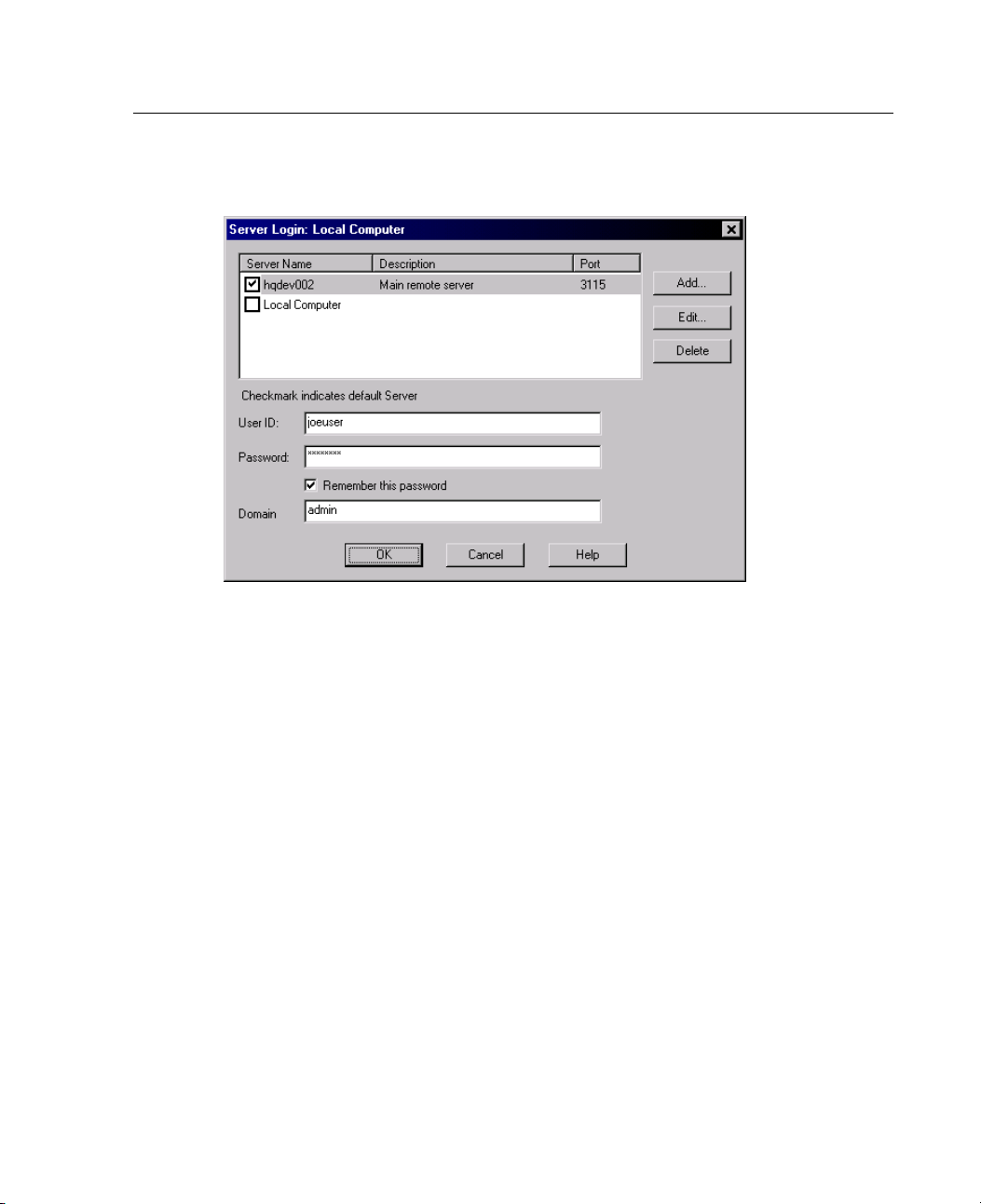
63
Distributed An
Figure 4-1
ServerLogindialogbox
alysis Mode
You can add, modify, or delete remote servers in the list. Remote servers usually
require a user ID and a password, and a domain name may also be necessary. Contact
your sy
stem administrator for information about available servers, a user ID and
password, domain names, and other connection information.
You can select a default server and save the user ID, domain name, and password
ated with any server. You are automatically connected to the default server
associ
when you start a new session.
Adding and Editing Server Login Settings
Use the Server Login Settings dialog box to add or edit connection information for
e servers for use in distributed analysis mode.
remot
Page 90
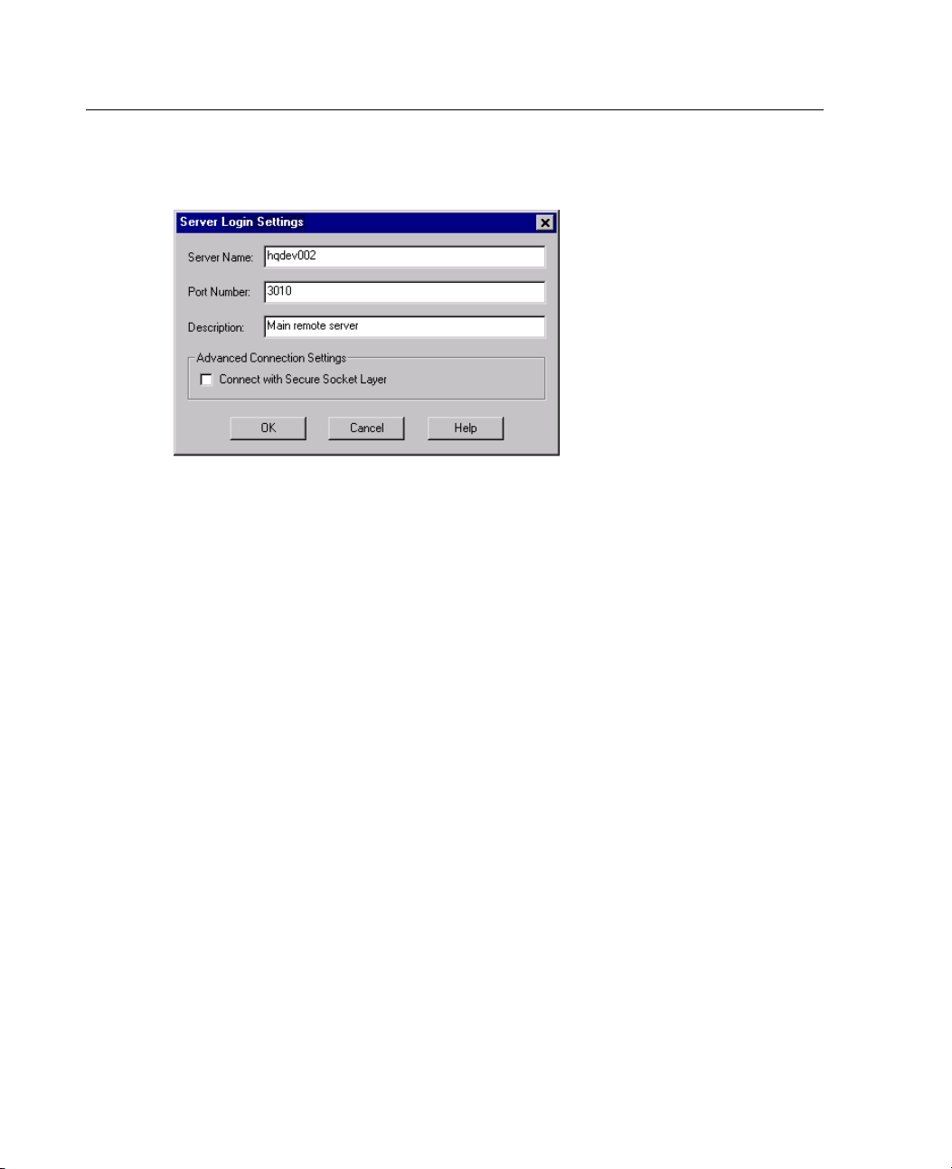
64
Chapter 4
Figure 4-2
Server Login Settings dialog box
Contact your system administrator for a list of available servers, port numbers for
the servers, and additional connection information. Do not use the Secure Sockets
Layer un
Name. A server “name” can be an alphanumeric name assigned to a computer (for
less instructed to do so by your administrator.
example, hqdev001) or a unique IP address assigned to a computer (for example,
202.123
.456.78).
Port Number. The port number is the port that the server software uses for
communications.
tion.
Descrip
Connect with Secure Sockets Layer. Secure Sockets Layer (SSL) encrypts requests
Enter an optional description to display in the servers list.
for distributed analysis when they are sent to the remote SPSS server. Before you
use SSL
, check with your administrator. SSL must be configured on your desktop
computer and the server for this option to be enabled.
Page 91

65
Distributed An
To Select, Switch, or Add Servers
E From the menus choose:
File
Switch Server...
To select a default server:
E In the server list, select the box next to the server that you want to use.
E Enter the user ID, domain name, and password provided by your administrator.
Note: You are automatically connected to the default server when you start a new
session.
To s witch to
E Select the
E Enter your
another server:
server from the list.
user ID, domain name, and password (if necessary).
Note: When you switch servers during a session, all open windows are closed. You
will be prompted to save changes before the windows are closed.
alysis Mode
Toaddaserver:
E Get the server connection information from your administrator.
E Click Add to open the Server Login Settings dialog box.
E Enter the connection information and optional settings and click OK.
To edit a server:
E Get the revised connection information from your administrator.
E Click Edit to open the Server Login Settings dialog box.
E Enter the changes and click OK.
Page 92
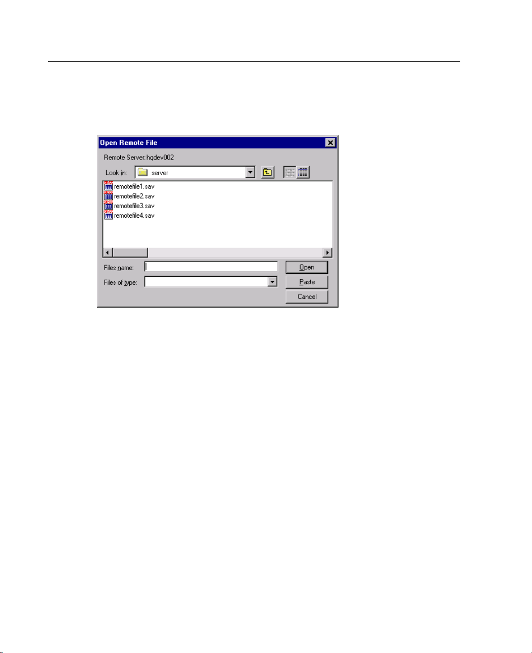
66
Chapter 4
Opening Data Files from a Remote Server
Figure 4-3
Open Remote F
ile dialog box
In distributed analysis mode, the Open Remote File dialog box replaces the standard
Open File dialog box.
The list of available files, folders, and drives is dependent on what is available
on or from the remote server. The current server name is indicated at the top of
the dialog box.
You will not have access to files on your local computer in distributed analysis
mode unless you specify the drive as a shared device or the folders containing
your data files as shared folders.
If the server is running a different operating system (for example, you are running
Windows and the server is running UNIX), you probably won't have access to
local data files in distributed analysis mode even if they are in shared folders.
Only one data file can be open at a time. The current data file is automatically closed
when a new data file is opened. If you want to have multiple data files open at the
same time, you can start multiple sessions.
To Open Data Files from a Remote Server
E If you aren't already connected to the remote server, log in to the remote server.
Page 93
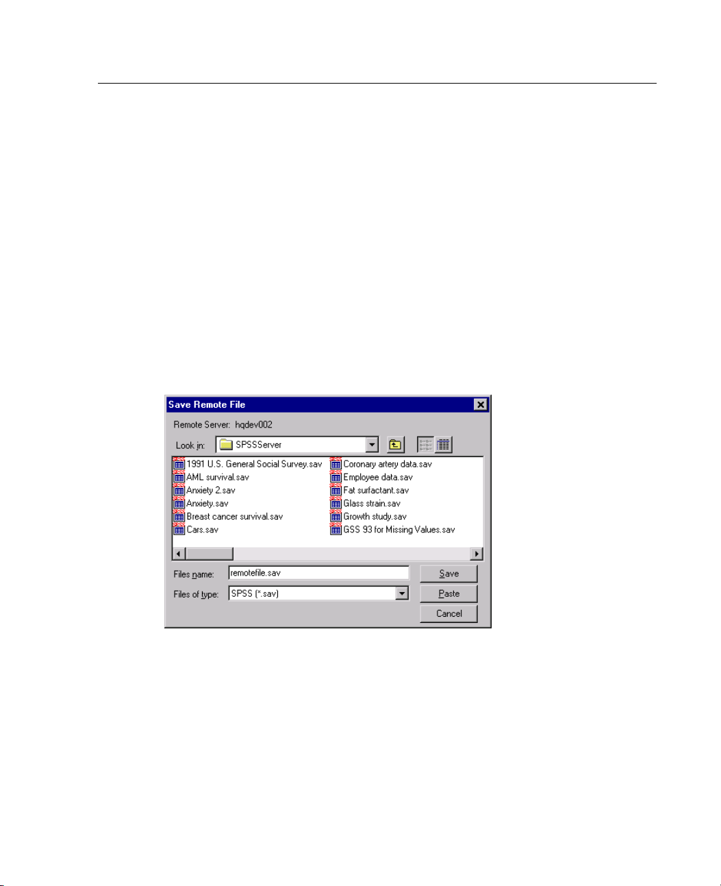
67
E
Depending on the type of data file that you want to open, from the menus choose:
File
Open
Data...
or
File
Open Database
or
File
Read Text Dat
a...
Saving Data Files from a Remote Server
Figure 4-4
Save Remote File dialog box
Distributed An
alysis Mode
Indistributedanalysismode,theSaveRemoteFiledialogboxreplacesthestandard
Save File dialog box.
The list of available folders and drives is dependent on what is available on or from
theremoteserver.Thecurrentservernameis indicated at the top of the dialog box.
You will not have access to folders on your local computer unless you specify the
drive as a shared device and the folders as shared folders. If the server is running a
different operating system (for example, you are running Windows and the server is
running UNIX), you probably will not have access to local data files in distributed
Page 94

68
Chapter 4
analysis mode even if they are in shared folders. Permissions for shared folders must
include the ability to write to the folder if you want to save data files in a local folder.
To Save Data
E Make the Da
E From the me
File
Save (or Save As...)
Data File Ac
The view of d
and the network is based on the computer you are currently using to process
commands and run procedures—which is not necessarily the computer in front of you.
Local anal
data files, folders, and drives that you see in the file access dialog box (for opening
data files) is similar to what you see in other applications or in the Windows Explorer.
You can se
folders on mounted network drives that you normally see.
Distributed analysis mode. When you use another computer as a “remote server” to
run comma
the view from the perspective of the remote server computer. Although you may
see familiar folder names such as Program Files anddrivessuchasC,theseare
not the f
remote server.
Files from a Remote Server
ta Editor the active window.
nus choose:
cess in Local and Distributed Analysis Mode
ata files, folders (directories), and drives for both your local computer
ysis mode.
e all of the data files and folders on your computer and any files and
nds and procedures, the view of data files, folders, and drives represents
olders and drives on your computer; they are the folders and drives on the
When you use your local computer as your “server,” the view of
Page 95
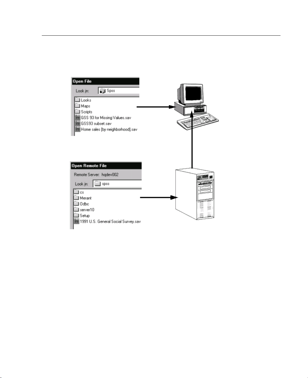
69
Figure 4-5
Local and remote views
Local View
Remote View
Distributed An
alysis Mode
tributed analysis mode, you will not have access to data files on your local
In dis
computer unless you specify the drive as a shared device or the folders containing
your data files as shared folders. If the server is running a different operating system
xample, if you are running Windows and the server is running UNIX), you
(for e
probably won't have access to local data files in distributed analysis mode even
iftheyareinsharedfolders.
ributed analysis mode is not the same as accessing data files that reside on
Dist
another computer on your network. You can access data files on other network
devices in local analysis mode or in distributed analysis mode. In local mode, you
ss other devices from your local computer. In distributed mode, you access other
acce
network devices from the remote server.
Page 96

70
Chapter 4
If you're not sure if you're using local analysis mode or distributed analysis mode,
look at the title bar in the dialog box for accessing data files. If the title of the
dialog box c
Server: [server name]
ontains the word Remote (as in
appears at the top of the dialog box, you're using distributed
Open Remote File), or if the text Remote
analysis mode.
Note:Thisa
ffects only dialog boxes for accessing data files (for example, Open D ata,
Save Data, Open Database, and Apply Data Dictionary). For all other file types (for
example, Viewer files, syntax files, and script files), the local view is always used.
To Set Shar
E In My Comp
E On the Fil
E Click the
ing Permissions for a Drive or Folder
, click the folder (directory) or drive that you want to share.
uter
e menu, click
Sharing tab, and then click Shared As.
Properties.
For more information about sharing drives and folders, see the Help for your
operating system.
Availability of Procedures in Distributed Analysis Mode
In distributed analysis mode, only procedures installed on both your local version
andtheversionontheremoteserverare available. You cannot use procedures
d on the server that are not also installed on your local version, and you
installe
cannot use procedures installed on your local version that are not also installed on
theremoteserver.
While th
components installed locally that are not available on the remote server. If this is the
case, switching from your local computer to a remote server will result in the removal
of the af
will result in errors. Switching back to local mode will restore all affected procedures.
e latter situation may be unlikely, it is possible that you may have optional
fected procedures from the menus, and the corresponding command syntax
Page 97

71
Using UNC Path Specifications
With the Windows NT server version of SPSS, relative path specifications for data
files are relative to the current server in distributed analysis mode, not relative to
your local c
c:\mydocs\mydata.sav does not point to a directory and file on your C drive; it points
to a directory and file on the r emote server's hard drive. If the directory and/or file do
not exist o
GET FILE='c:\mydocs\mydata.sav'.
If you are using the Windows NT server version of SPSS, you can use universal
naming con
syntax. The general form of a UNC specification is:
\\servername\sharename\path\filename
Servername is the name of the computer that contains the data file.
Sharename is the folder (directory) on that computer that is designated as a
shared folder.
Path is any additional folder (subdirectory) path below the shared folder.
Filename is the name of the data file.
omputer. In practical terms, this means that a path specification such as
n the remote server, this will result in an error in command syntax, as in:
vention (UNC) specifications when accessing data files with command
Distributed An
alysis Mode
For example:
GET FILE='
If the comp
GET FILE='\\204.125.125.53\public\july\sales.sav'.
\\hqdev001\public\july\sales.sav'.
uter does not have a name assigned to it, you can use its IP address, as in:
Even with UNC path specifications, you can access data files only from devices and
folders de
signated as shared. When you use distributed analysis mode, this includes
data files on your local computer.
UNIX servers. On UNIX platforms, there is no equivalent of the UNC path, and all
director
y paths must be absolute paths that start at the root of the server; relative paths
are not allowed. For example, if the data file is located in /bin/spss/data and the
current directory is also /bin/spss/data,
specify t
GET FILE='/bin/data/spss/sales.sav'.
he entire path, as in:
GET FILE='sales.sav' is not valid; you must
Page 98

Page 99
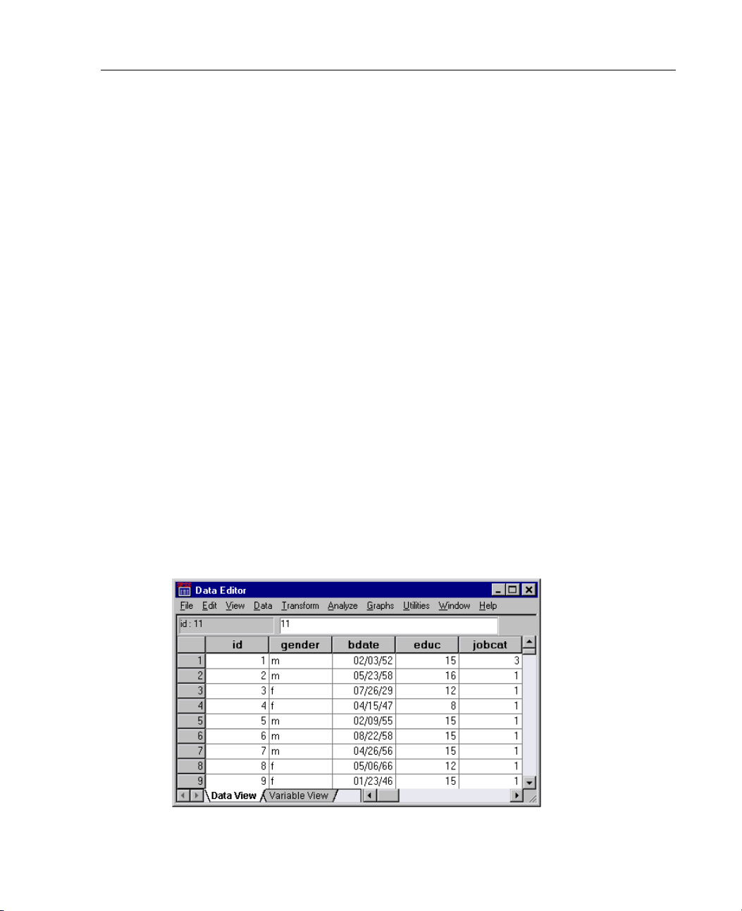
Data Editor
The Data Editor provides a convenient, spreadsheet-like method for creating and
editing dat
session.
The Data Editor provides two views of your data:
Data view. Displays the actual data values or defined value labels.
Variable view. Displays variable definition information, including defined variable
a files. The Data Editor window opens automatically when you start a
and value l
level (nominal, ordinal, or scale), and user-defined missing values.
abels, data type (for example, string, date, and numeric), measurement
Chapter
5
In both vie
Data View
Figure 5-1
Data view
ws, you can add, change, and delete information contained in the data file.
73
Page 100
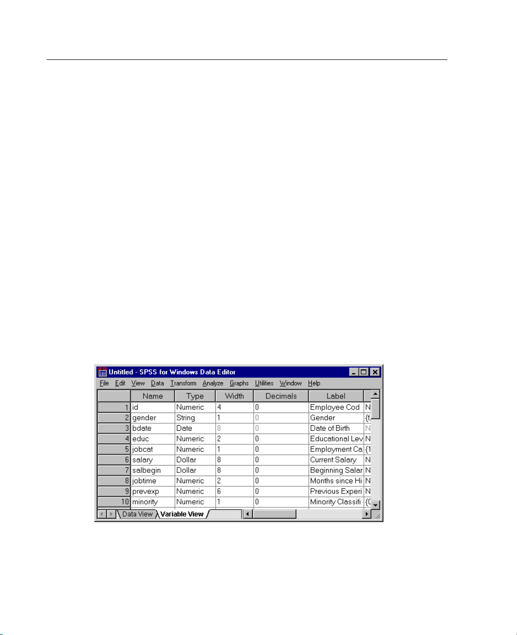
74
Chapter 5
Many of the features of the Data view are similar to those found in spreadsheet
applications. There are, however, several important distinctions:
Rows are cases. Each row represents a case or an observation. For example, each
individual respondent to a questionnaire is a case.
Columns are variables. Each column represents a variable or characteristic being
measured. F
Cells cont
or example, each item on a questionnaire is a variable.
ain values. Each cell contains a single value of a variable for a case. The
cell is the intersection of the case and the variable. Cells contain only data values.
Unlike spreadsheet programs, cells in the Data Editor cannot contain formulas.
The data file is rectangular. The dimensions of the data file are determined by
the number o
f cases and variables. You can enter data in any cell. If you enter
data in a cell outside the boundaries of the defined data file, the data rectangle
is extended to include any rows and/or columns between that cell and the file
boundarie
s. There are no “empty” cells within the boundaries of the data file. For
numeric variables, blank cells are converted to the system-missing value. For
string variables, a blank is considered a valid value.
Variable
View
Figure 5-2
Variable view
 Loading...