

Page 1
™
SPSS Advan
ced Models
12.0
Page 2
For more information about SPSS®software products, please visit our Web site at
http://www.
SPSS Inc.
233 South Wacker Drive, 11th Floor
Chicago, IL 60
Tel: (312) 651-3000
Fax: (312) 651-3668
SPSS is a regis
of SPSS Inc. for its proprietary computer software. No material describing such
software may be produced or distributed without the written permission of the
owners of the
the published materials.
The SOFTWARE and documentation are provided with RESTRICTED RIGHTS.
Use, duplica
in subdivision (c) (1) (ii) of The Rights in Technical Data and Computer Software
clause at 52.227-7013. Contractor/manufacturer is SPSS Inc., 233 South Wacker
Drive, 11th
General notice: Other product names mentioned herein are used for identification
purposes only and may be trademarks of their respective companies.
TableLook i
Windows is a registered trademark of Microsoft Corporation.
DataDirect, DataDirect Connect, INTERSOLV, and SequeLink are registered
trademarks
Portions of this product were created using LEADTOOLS © 1991-2000, LEAD
Technologies, Inc. ALL RIGHTS RESERVED.
LEAD, LEADTO
Technologies, Inc.
Portions of this product were based on the work of the FreeType Team
(http://ww
SPSS Advanced Models™ 12.0
Copyright © 2003 by SPSS Inc.
All rights re
Printed in the United States of America.
No part of this publication may be reproduced, stored in a retrieval system, or
transmitted
recording, or otherwise, without the prior written permission of the publisher.
spss.com or contact
606-6412
tered trademark and the other product names are the trademarks
trademark and license rights in the software and the copyrights in
tion, or disclosure by the Government is subject to restrictions as set forth
Floor, Chicago, IL 60606-6412.
s a trademark of SPSS Inc.
of DataDirect Technologies.
OLS, and LEADVIEW are registered trademarks of LEAD
w.freetype.org).
served.
, in any form or by any means, electronic, mechanical, photocopying,
Page 3
Preface
SPSS 12.0 is a powerful software package for microcomputer data management and
analysis. The Advanced Models option is an add-on enhancement that provides
nal statistical analysis techniques. The procedures in Advanced Models must
additio
be used with the SPSS 12.0 Base and are completely integrated into that system.
The Advanced Models option includes procedures for:
Multivariate and repeated measures general linear models
Variance components analysis
Linear mixed models
Loglinear analysis, including model selection (hierarchical), general loglinear
models,
Ordina
Surviv
Cox regression
and logit loglinear models
l regression analysis
al analysis, including life tables, Kaplan-Meier survival analysis, and
Installation
To install Advanced Models, follow the instructions for adding and removing features
in the installation instructions supplied with the SPSS Base. (To start, double-click on
the SPS
SSetupicon.)
iii
Page 4
Compatibility
SPSS is designed to run on many computer systems. See the materials that came with
your system for specific information on minimum and recommended requirements.
Serial Numbers
Your serial number is your identification number with SPSS Inc. You will need
this serial number when you contact SPSS Inc. for information regarding support,
payment, or
an upgraded system. The serial number was provided with your Base
system.
Customer Se
If you have
rvice
any questions concerning your shipment or account, contact your local
office, listed on the SPSS Web site at http://www.spss.com/worldwide.Pleasehave
your serial number ready for identification.
Training Seminars
SPSS Inc. provides both public and onsite training seminars. All seminars feature
hands-on workshops. Seminars will be offered in major cities on a regular basis. For
more info
rmation on these seminars, contact your local office, listed on the SPSS
Web site at http://www.spss.com/worldwide.
Technica
The servi
l Support
ces of SPSS Technical Support are available to registered customers.
Customers may contact Technical Support for assistance in using SPSS products
or for installation help for one of the supported hardware environments. To reach
Technic
al Support, see the SPSS Web site at http://www.spss.com, or contact your
local office, listed on the SPSS Web site at http://www.spss.com/worldwide.Be
prepared to identify yourself, your organization, and the serial number of your system.
iv
Page 5
Additional Publications
Additional copies of SPSS product manuals may be purchased directly from SPSS
Inc. Visit our Web site at http://www.spss.com/estore, or contact your local SPSS
office, list
ed on the SPSS Web site at http://www.spss.com/worldwide. For telephone
orders in the United States and Canada, call SPSS Inc.. at 800-543-2185. For
telephone orders outside of North America, contact your local office, listed on the
SPSS Web sit
e.
The SPSS Statistical Procedures Companion, by Marija Norušis, is being prepared
for publication by Prentice Hall. It contains overviews of the procedures in the SPSS
Base, plus
Logistic Regression, General Linear Models, and Linear Mixed Models.
Further information will be available on the SPSS Web site at http://www.spss.com
Store, select your country, and click Books).
(click
Tell Us Your Thou ghts
Your comments are important. Please send us a letter and let us know about your
experiences with SPSS p roducts. We especially like to hear about new and interesting
applicat
ions using the SPSS system. Please send e-mail to [email protected] or
write to SPSS Inc., Attn.: Director of Product Planning, 233 South Wacker Drive,
11th Floor, Chicago, IL 60606-6412.
About This Manual
This manual documents the graphical user interface for the procedures included in
the Advanced Models module. Illustrations of dialog boxes are taken from SPSS
for Wind
ows. Dialog boxes in other operating systems are similar. The Advanced
Models command syntax is included in the SPSS 12.0 Command Syntax Reference,
available on the product CD-ROM.
Contacting SPSS
If you would like t o be on our mailing list, contact one of our offices, listed on
our Web site at http://www.spss.com/worldwide. We will send you a copy of our
tter and let you know about SPSS Inc. activities in your area.
newsle
v
Page 6
Page 7
Contents
1 GLM Multivar
GLMMultivariateDataConsiderations............................ .2
ObtainingGLMMultivariateTables............................... .3
iate Analysis 1
2 GLM Repeated Measures 17
GLMRepeatedMeasuresDataConsiderations..................... .18
GLMRepeatedMeasuresDefineFactors......................... .20
DefiningFactorsforGLMRepeatedMeasures..................... .21
ObtainingGLMRepeatedMeasuresTables........................ .22
3 Variance Components Analysis 35
VarianceComponentsDataConsiderations ....................... .36
ObtainingVarianceComponentsTables .......................... .36
4 Linear Mixed Models 43
LinearMixedModelsDataConsiderations........................ .44
Linear Mixed Models Select Subjects/Repeated Variables . . . . . . . . . . . . . 44
Selecting Subjects/Repeated Variables for Linear Mixed Models . . . . . . . . 46
vii
Page 8
ObtainingaLinearMixedModelsAnalysis........................ .47
5 Model Selection Loglinear Analysis 59
Model Selection Loglinear Analysis Da ta Considerations . . . . . . . . . . . . . . 59
ObtainingaModelSelectionLoglinearAnalysis.................... .60
6 General Loglinear Analysis 65
GeneralLoglinearAnalysisDataConsiderations.................... .66
ObtainingaGeneralLoglinearAnalysis........................... .66
7 Logit Loglinear Analysis 73
LogitLoglinearAnalysisDataConsiderations...................... .74
ObtainingaLogitLoglinearAnalysis............................. .74
8 Ordinal Regression 81
OrdinalRegressionDataConsiderations.......................... .82
ObtaininganOrdinalRegression ............................... .82
9 Life Tables 91
LifeTablesDataConsiderations................................ .92
viii
Page 9
CreatingLifeTables ......................................... .93
10 Kaplan-Meier Survival Analysis 97
Kaplan-MeierDataConsiderations.............................. .97
ObtainingaKaplan-MeierSurvivalAnalysis....................... .98
11 Cox Regression Analysis 105
CoxRegressionDataConsiderations ........................... .105
ObtainingaCoxRegressionAnalysis ........................... .106
12 Computing Time-Dependent Covariates 113
ComputingaTime-DependentCovariate......................... .114
Appendices
A Categorical Variable Coding Schemes 117
Deviation................................................ .117
Simple .................................................. .118
Helmert ................................................. .119
Difference ............................................... .120
Polynomial............................................... .120
ix
Page 10
Repeated................................................ .121
Special ................................................. .122
Indicator ................................................ .123
B Covariance Structures 125
Index 131
x
Page 11
Chapter
1
GLM Multivar
The GLM Multivariate procedure provides regression analysis and analysis of
variance fo
covariates. The factor variables divide the population into groups. Using this general
linear model procedure, you can test null hypotheses about the effects of factor
variables
variables. You can investigate interactions between factors as well as the effects of
individual factors. In addition, the effects of covariates and covariate interactions
with fact
variables are specified as covariates.
Both balanced and unbalanced models can be tested. A design is balanced if
each cell
the sums of squares due to the effects in the model and error sums of squares
are in matrix form rather than the scalar form found in univariate analysis. These
matrice
than one dependent variable is specified, the multivariate analysis of variance using
Pillai's trace, Wilks' lambda, Hotelling's trace, and Roy's largest root criterion with
approx
for each dependent variable. In addition to testing hypotheses, GLM Multivariate
produces estimates of parameters.
Common
Additionally, after an overall F test has shown significance, you can use post hoc
tests to evaluate differences among specific means. Estimated marginal means give
estim
(interaction plots) of these means allow you to visualize some of the relationships
easily. The post hoc multiple comparison tests are performed for each dependent
varia
r multiple dependent variables by one or more factor variables or
on the means of various groupings of a joint distribution of dependent
ors can be included. For regression analysis, the independent (predictor)
in the model contains the same number of cases. In a multivariate model,
s are called SSCP (sums-of-squares and cross-products) matrices. If more
imate F statistic are provided as well as the univariate analysis of variance
ly used aprioricontrasts are available to perform hypothesis testing.
ates of predicted mean values for the cells in the model, and profile plots
ble separately.
iate Analysis
1
Page 12
2
Chapter 1
Residuals, predicted values, Cook's distance, and leverage values can be saved as
new variables in your data file for checking assumptions. Also available are a residual
SSCP matrix
, which is a square matrix of sums of squares and cross-products of
residuals, a residual covariance matrix, which is the residual SSCP matrix divided by
the degrees of freedom of the residuals, and the residual correlation matrix, which is
the standa
rdized form of the residual covariance matrix.
WLS Weight allows you to specify a variable used to give observations different
weights for a weighted least-squares (WLS) analysis, perhaps to compensate for
different
Example. A manufacturer of plastics measures three properties of plastic film: tear
precision of measurement.
resistance, gloss, and opacity. Two rates of extrusion and two different amounts of
additive a
re tried, and the three properties are measured under each combination of
extrusion rate and additive amount. The manufacturer finds that the extrusion rate and
the amount of additive individually produce significant results but that the interaction
of the two
Methods. Type I, Type II, Type III, and Type IV sums of squares can be used to
factorsisnotsignificant.
evaluate different hypotheses. Type III is the default.
ics.
Statist
Post hoc range tests and multiple comparisons: least significant
difference, Bonferroni, Sidak, Scheffé, Ryan-Einot-Gabriel-Welsch multiple F,
Ryan-Einot-Gabriel-Welsch multiple range, Student-Newman-Keuls, Tukey's
y significant difference, Tukey's-b, Duncan, Hochberg's GT2, Gabriel, Waller
honestl
Duncan t test, Dunnett (one-sided and two-sided), Tamhane's T2, Dunnett's T3,
Games-Howell, and Dunnett's C. Descriptive statistics: observed means, standard
ions, and counts for all of the dependent variables in all cells; the Levene test
deviat
for homogeneity of variance; Box's M test of the homogeneity of the covariance
matrices of the dependent variables; and Bartlett's test of sphericity.
Spread-versus-level, residual, and profile (interaction).
Plots.
GLM Multivariate Data Considerations
Data. The dependent variables should be quantitative. Factors are categorical and
ve numeric values or string values of up to eight characters. Covariates are
can ha
quantitative variables that are related to the dependent variable.
Page 13
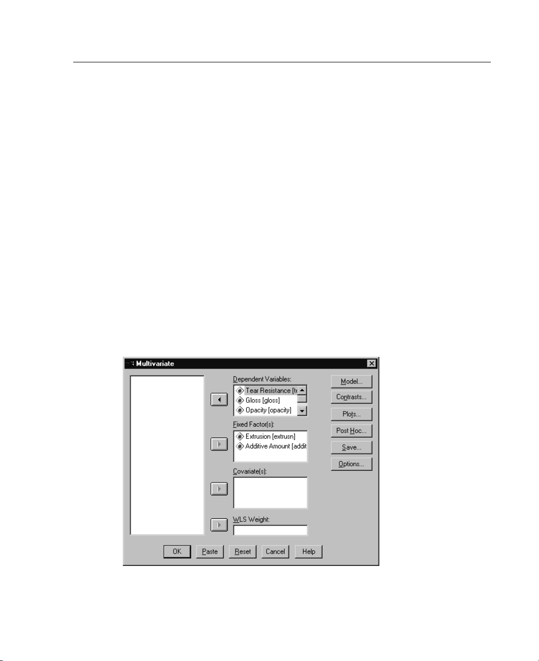
3
Obtainin
E From the
GLM Multivaria
Assumptions. For dependent variables, the data are a random sample of vectors
te Analysis
from a multivariate normal population; in the population, the variance-covariance
matrices fo
r all cells are the same. Analysis of variance is robust to departures from
normality, although the data should be symmetric. To check assumptions, you can use
homogeneity of variances tests (including Box's M) and spread-versus-level plots.
You can als
Related procedures. Use the Explore procedure to examine the data before doing an
o examine residuals and residual plots.
analysis of variance. For a single dependent variable, use GLM Univariate. If you
measured t
he same dependent variables on several occasions for each subject, use
GLM Repeated Measures.
g GLM Multivariate Tables
menus choose:
Analyze
General Linear Model
Multivariate...
Figure 1-
Multivar
1
iate dialog box
E Sele
ct at least two dependent variables.
Page 14
4
Chapter 1
Optionally, you can specify Fixed Factor(s), Covariate(s), and WLS Weight.
GLM Multiva
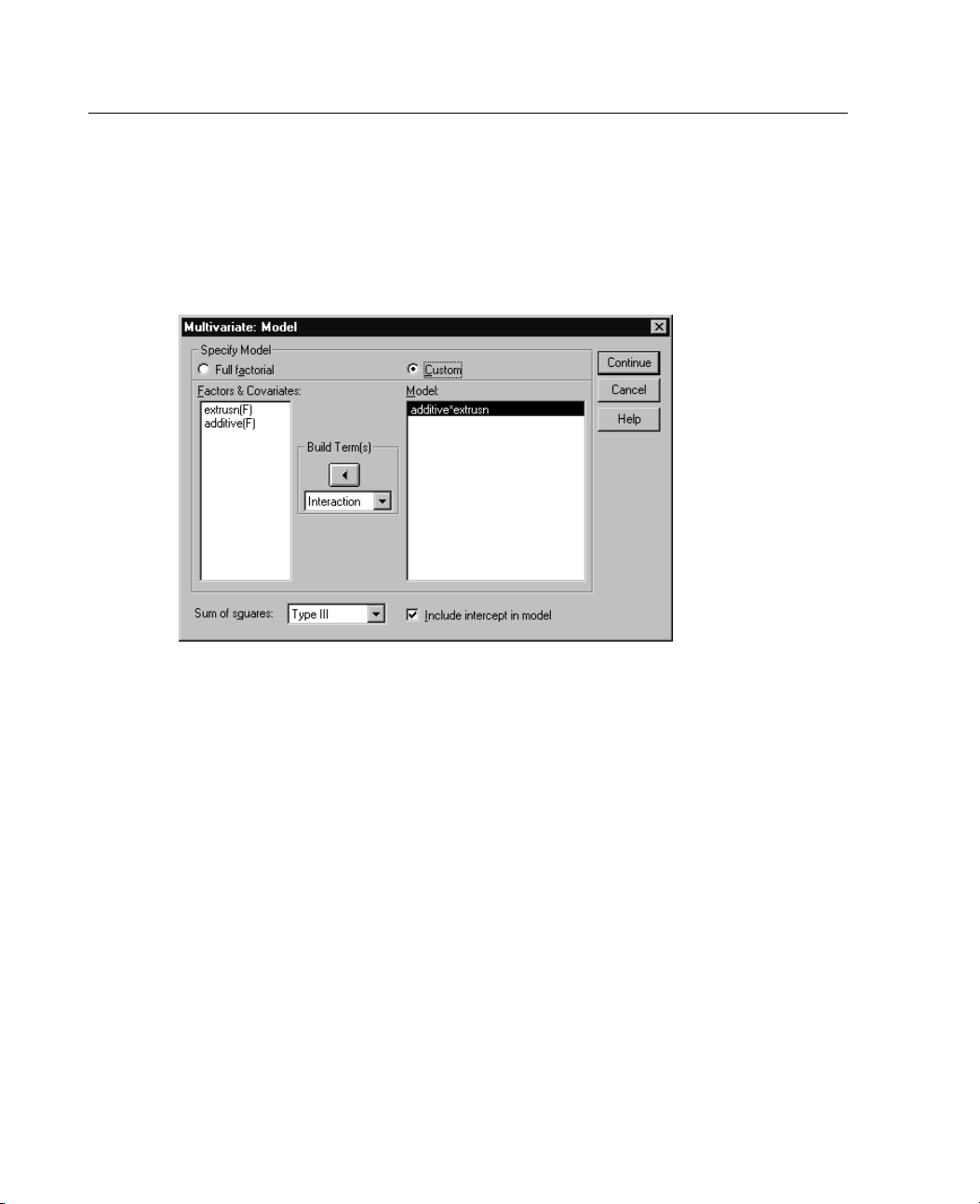
Figure 1-2
Multivariate Model dialog box
Specify Model. A full factorial model contains all factor main effects, all covariate
main effects, and all factor-by-factor interactions. It does not contain covariate
interactions. Select
factor-by-covariate interactions. You must indicate all of the terms to be included
in the model.
riate Model
Custom to specify only a subset of interactions or to specify
Factors and Covariates. The factors and covariates are listed with (F) for fixed factor
and (C) for covariate.
Model. The model depends on the nature of your data. After selecting Custom,you
can select the main effects and interactions that are of interest in your analysis.
Sum of squares. The method of calculating the sums of squares. For balanced or
unbalanced models with no missing cells, the Type III sum-of-squares method is
the most commonly used type.
Include intercept in model. The intercept is usually included in the model. If you can
assume that the data pass through the origin, you can exclude the intercept.
Page 15
5
GLM Multivaria
Build Terms
For the selected factors and covariates:
Interaction. Creates the highest-level interaction term of all selected variables. This is
the default
Main effects. Creates a main-effects term for each variable selected.
All 2-way. Creates all possible two-way interactions of the selected variables.
All 3-way. C
All 4-way. Creates all possible four-way interactions of the selected variables.
All 5-way. Creates all possible five-way interactions of the selected variables.
Sums of Squa
For the mode
.
reates all possible three-way interactions of the selected variables.
res
l, you can choose a type of sum of squares. Type III is the most
commonly used and is the default.
Type I. This method is also known as the hierarchical decomposition of the
sum-of-squ
ares method. Each term is adjusted only for the term that precedes it in the
model. The Type I sum-of-squares method is commonly used for:
A balanced ANOVA model in which any main effects are specified before any
first-ord
er interaction effects, any first-order interaction effects are specified
before any second-order interaction effects, and so on.
A polynomial regression model in which any lower-order terms are specified
before any higher-order terms.
Apurelynestedmodelinwhichthefirst-specifiedeffectisnestedwithinthe
second-sp
ecified effect, t he second-specified effect is nested within the third, and
so on. (This form of nesting can be specified only by using syntax.)
te Analysis
Type II. T
his method calculates the sums of squares of an effect in the model adjusted
for all other “appropriate” effects. An appropriate effect is one that corresponds to all
effects that do not contain the effect being examined. The Type II sum-of-squares
method is
A balanc
Any mode
commonlyusedfor:
ed ANOVA model.
l that has main factor effects only.
Page 16
6
Chapter 1
Any regression model.
A purely nested design. (This form of nesting can be specified by using syntax.)
Type III. This method, the default, calculates the sums of squares of an effect in the
design as the
sums of squares adjusted for any other effects that do not contain
it and orthogonal to any effects (if any) that contain it. The Type III sums of
squares have one major advantage in that they are invariant with respect to the cell
frequencie
saslongasthegeneralformofestimability remains constant. Therefore,
this type is often considered useful for an unbalanced model with no missing
cells. In a factorial design with no missing cells, this method is equivalent to the
Yates' wei
ghted-squares-of-means technique. The Type III sum-of-squares method
is commonly used for:
AnymodelslistedinTypeIandTypeII.
Any balanced or unbalanced model with no empty cells.
Type IV. This method is designed for a situation in which there are missing cells. For
any effect
F in the design, if F is not contained in any other effect, then Type IV =
Type III = Type II. When F is contained in other effects, Type IV distributes the
contrasts being made among the parameters in F to all higher-level effects equitably.
The Type I
Any mode
Any bala
V sum-of-squares method is commonly used for:
ls listed in Type I and Type II.
nced model or unbalanced model with empty cells.
GLM Multivariate Contrasts
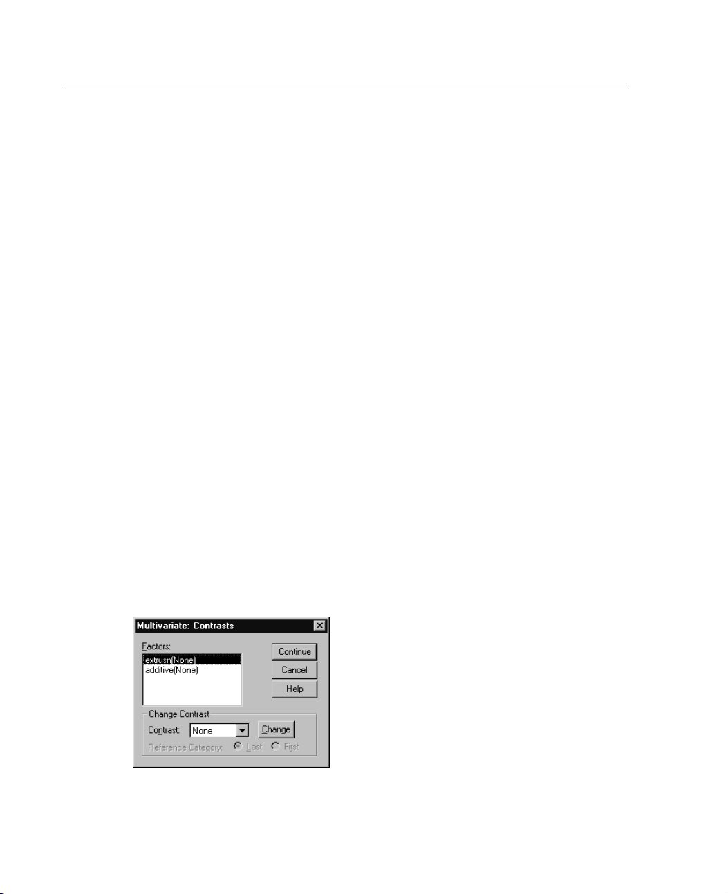
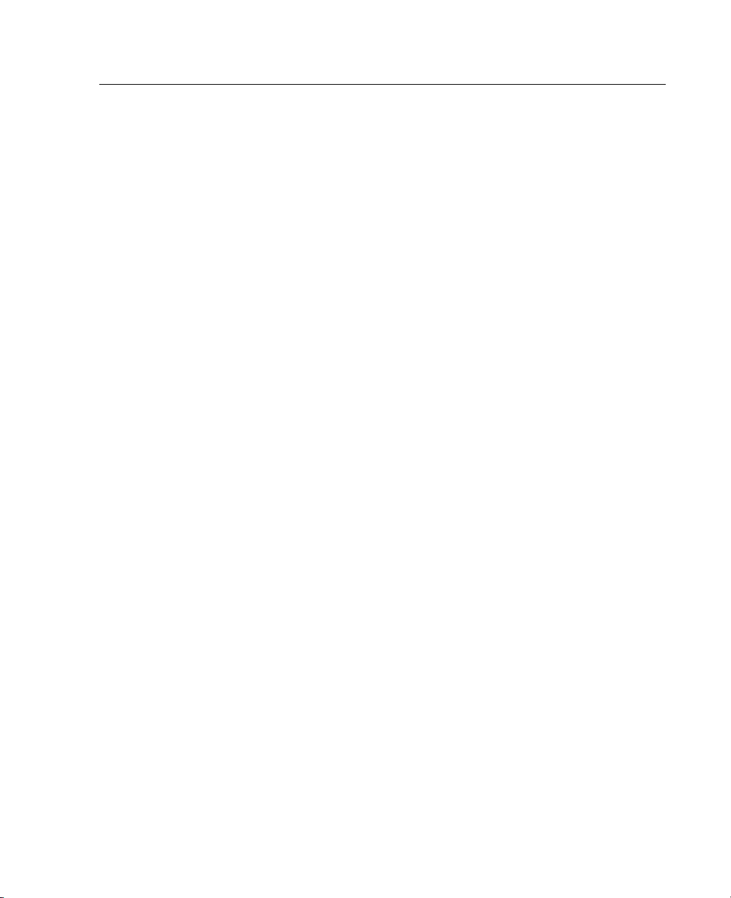
Figure 1-3
Multivariate Contrasts dialog box
Page 17
7
GLM Multivaria
Contrasts are used to test whether the levels of an effect are significantly different
from one another. You can specify a contrast for each factor in the model. Contrasts
represent l
inear combinations of the parameters.
Hypothesis testing is based on the null hypothesis LBM = 0,whereL is the contrast
coefficientsmatrix, M is the identity matrix, which has dimension equal to the number
of dependen
tvariables,andB is the parameter vector. When a contrast is specified,
SPSS creates an L matrix such that the columns corresponding to the factor match the
contrast. The remaining columns are adjusted so that the L matrix is estimable.
In additio
n to the univariate test using F statistics and the Bonferroni-type
simultaneous confidence intervals based on Student's t distribution for the contrast
differences across all dependent variables, the multivariate tests using Pillai's trace,
Wilks' lam
bda, Hotelling's trace, and Roy's largest root criteria are provided.
A vailable contrasts are deviation, simple, difference, Helmert, repeated, and
polynomial. For deviation contrasts and simple contrasts, you can choose whether the
referenc
e category is the last or first category.
Contrast Types
Deviation. Compares the mean of each level (except a reference category) to the mean
of all of the levels (grand mean). The levels of the factor can be in any order.
te Analysis
Simple. C
ompares the mean of each level to the mean of a specified level. This
type of contrast is useful when there is a control group. You can choose the first or
last category as the reference.
nce.
Differe
Compares the mean of each level (except the first) to the mean of previous
levels. (Sometimes called reverse Helmert contrasts.)
Helmert. Compares the mean of each level of the factor (except the last) to the mean
of subse
Repeated. Compares the mean of each level (except the last) to the mean of the
quent levels.
subsequent level.
ial.
Polynom
Compares the linear effect, quadratic effect, cubic effect, and so on. The
first degree of freedom contains the linear effect across all categories; the second
degree of freedom, the quadratic effect; and so on. These contrasts are often used
mate polynomial trends.
to esti
Page 18
8
Chapter 1
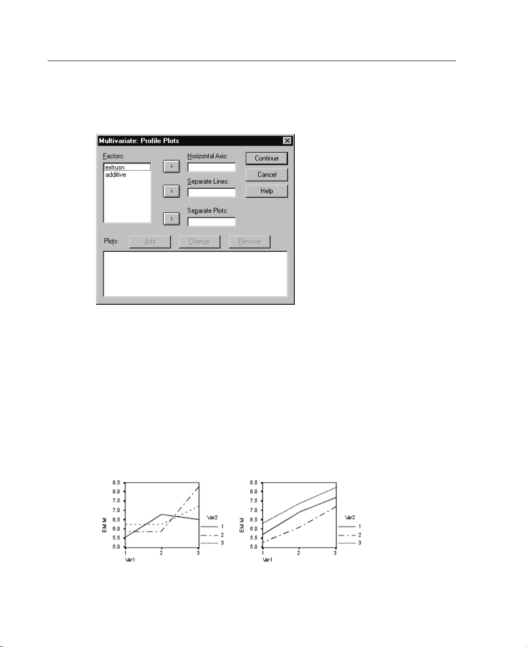
GLM M ultivariate Profile Plots
Figure 1-4
Multivariat
e Profile Plots dialog box
Profile plots (interaction plots) are useful for comparing marginal means in your
model. Profile plots are created for each dependent variable. A profile plot is a
line plot in which each point indicates the estimated marginal mean of a dependent
variable (adjusted for covariates) at one level of a factor. The levels of a second factor
can be used to make separate lines. Each level in a third factor can be used to create a
separate plot. All fixed factors are available for plots.
A profile plot of one factor shows whether the estimated marginal means are
increasing or decreasing across levels. For two or more factors, parallel lines indicate
that there is no interaction between factors, which means that you can investigate the
levels of only one factor. Lines that cross each other indicate an interaction.
Figure 1-5
Nonparallel plot (left) and parallel plot (right)
Page 19
9
GLM Multivaria
After a plot is specified by selecting factors for the horizontal axis, and optionally,
factors for separate lines and separate plots, the plot must be listed in the Plots list.
GLM Multivariate Post Hoc Multiple Comparisons for Observed Means
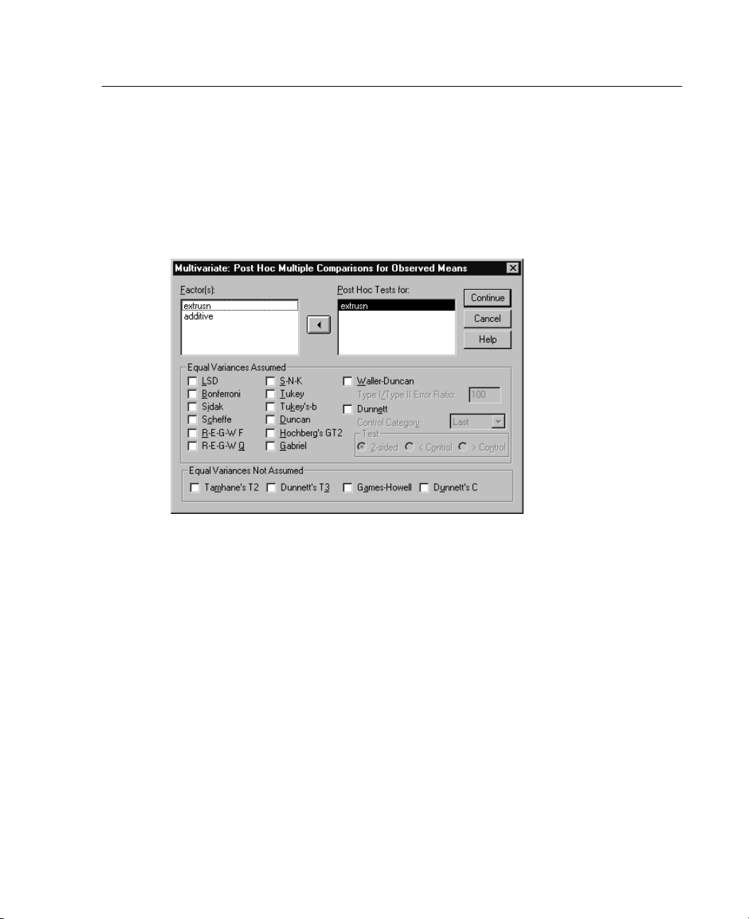
Figure 1-6
Post H oc Mul
tiple Comparisons for Observed Means dialog box
te Analysis
Post ho
c multiple comparison tests.
Once you have determined that differences exist
among the means, post hoc range tests and pairwise multiple comparisons can
determine which means differ. Comparisons are made on unadjusted values. These
re used for between-subjects factors only. The post hoc multiple comparison
tests a
tests are performed for each dependent variable separately.
The Bonferroni and Tukey's honestly significant difference tests are commonly
used m
ultiple comparison tests. The Bonferroni test, based on Student's t statistic,
adjusts the observed significance level for the fact that multiple comparisons are
made. Sidak's t test also adjusts the significance level and provides tighter bounds
he Bonferroni test. Tukey's honestly significant difference test uses the
than t
Studentized range statistic to make all pairwise comparisons between groups and sets
the experimentwise error rate to the error rate for the collection for all pairwise
arisons. When testing a large number of pairs of means, Tukey's honestly
comp
significant difference test is more powerful than the Bonferroni test. For a small
number of pairs, Bonferroni is more powerful.
Page 20
10
Chapter 1
Hochberg's GT2 is similar to Tukey's honestly significant difference test, but the
Studentized maximum modulus is used. Usually, Tukey's test is more powerful.
Gabriel's p
airwise comparisons test also uses the Studentized maximum modulus
and is generally more powerful than Hochberg's GT2 when the cell sizes are unequal.
Gabriel's test may become liberal when the cell sizes vary greatly.
Dunnett's p
airwise multiple comparison t test compares a set of treatments
against a single control mean. The last category is the default control category.
Alternatively, you can choose the first category. You can also choose a two-sided or
one-sided
test. To test that the mean at any level (except the control category) of the
factor is not equal to that of the control category, use a two-sided test. To test whether
the mean at any level of the factor is smaller than that of the control category, select
Likewise, to test whether the mean at any level of the factor is larger than that
.
Control
of the control category, select
> Control.
Ryan, Einot, Gabriel, and Welsch (R-E-G-W) developed two multiple step-down
range tes
ts. Multiple step-down procedures first test whether all means are equal.
If all means are not equal, subsets of means are tested for equality. R-E-G-W F is
based on an F test and R-E-G-W Q is based on the Studentized range. These tests
are more
powerful than Duncan's multiple range test and Student-Newman-Keuls
(which are also multiple step-down procedures), but they are not recommended
for unequal cell sizes.
When the
variances are unequal, use Tamhane's T2 (conservative pairwise
comparisons test based on a t test), Dunnett's T3 (pairwise comparison test based
on the Studentized maximum modulus), Games-Howell pairwise comparison
ometimes liberal), or Dunnett's C (pairwise comparison test based on the
test (s
Studentized range).
Duncan's multiple range test, Student-Newman-Keuls (S-N-K), and Tukey's-b
ge tests that rank group means and compute a range value. These tests are
are ran
not used as frequently as the tests previously discussed.
The Waller-Duncan t test uses a Bayesian approach. This range test uses the
nic mean of the sample size when the sample sizes are unequal.
harmo
The significance level of the Scheffé test is designed to allow all possible linear
combinations of group means to be tested, not just pairwise comparisons available in
eature. The result is that the Scheffé test is often more conservative than other
this f
tests, which means that a larger difference between means is required for significance.
<
Page 21
11
equivalent to multiple individual t tests between all pairs of groups. The disadvantage
of this test
multiple comparisons.
Tests displayed. Pairwise comparisons are provided for LSD, Sidak, Bonferroni,
Games and Ho
Homogeneous subsets for range tests are provided for S-N-K, Tukey's-b,Duncan,
R-E-G-W F, R-E-G-W Q, and Waller. Tukey's honestly significant difference test,
Hochberg'
tests and range tests.
GLM Multi
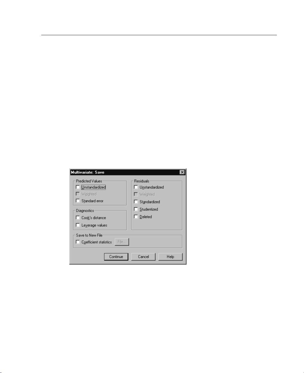
Figure 1-7
Multivariate Save dialog box
GLM Multivaria
The least significant difference (LSD) pairwise multiple comparison test is
is that no attempt is made to adjust the observed significance level for
well, Tamhane's T2 and T3, Dunnett's C, and Dunnett's T3.
s GT2, Gabriel's test, and Scheffé's test are both multiple comparison
variate Save
te Analysis
You can save values predicted by the model, residuals, and related measures as new
variables in the Data Editor. Many of these variables can be used for examining
assumptions about the data. To save the values for use in another SPSS session, you
must save the current data file.
Predicted Values. The values that the model predicts for each case. Unstandardized
predicted values and the standard errors of the predicted values are available. If a
WLS variable was chosen, weighted unstandardized predicted values are available.
Page 22
12
Chapter 1
Diagnostics. Measures to identify cases with unusual combinations of values for the
independent variables and cases that may have a large impact on the model. Ava ilable
are Cook's d
Cook's Dis
istance and uncentered leverage values.
tance.
A measure of how much the residuals of all cases would
change if a particular case were excluded from the calculation of the regression
coefficients. A large Cook's D indicates that excluding a case from computation
of the regr
Leverage V
Residuals. An unstandardized residual is the actual value of the dependent variable
ession statistics, changes the coefficients substantially.
alue.
The relative influence of each observation on the model's fit.
minus the value predicted by the model. Standardized, Studentized, and deleted
residuals
are also available. If a WLS variable was chosen, weighted unstandardized
residuals are available.
Unstandardized Residuals. The difference between an observed value and the
value pred
Weighted
icted by the model.
Residuals.
Weighted unstandardized residuals. Available only if a
WLS variable was previously selected.
Standardized. The residual divided by an estimate of its standard error.
Standardized residuals are also known as Pearson residuals.
Studentized Residual. The residual divided by an estimate of its standard deviation
that vari
es from case to case, depending on the distance of each case's values on
the independent variables from the means of the independent variables.
Deleted Residual. The residual for a case when that case is excluded from the
calculation of the regression coefficients. It is the difference between the value of
the depe
ndent variable and the adjusted predicted value.
Save to New File. Writes an SPSS data file containing a variance-covariance matrix of
the parameter estimates in the model. Also, for each dependent variable, there will
bearowo
f parameter estimates, a row of significance values for the t statistics
corresponding to the parameter estimates, and a row of residual degrees of freedom.
For a multivariate model, there are similar rows for each dependent variable. You can
s data in other SPSS procedures.
use thi
Page 23
13
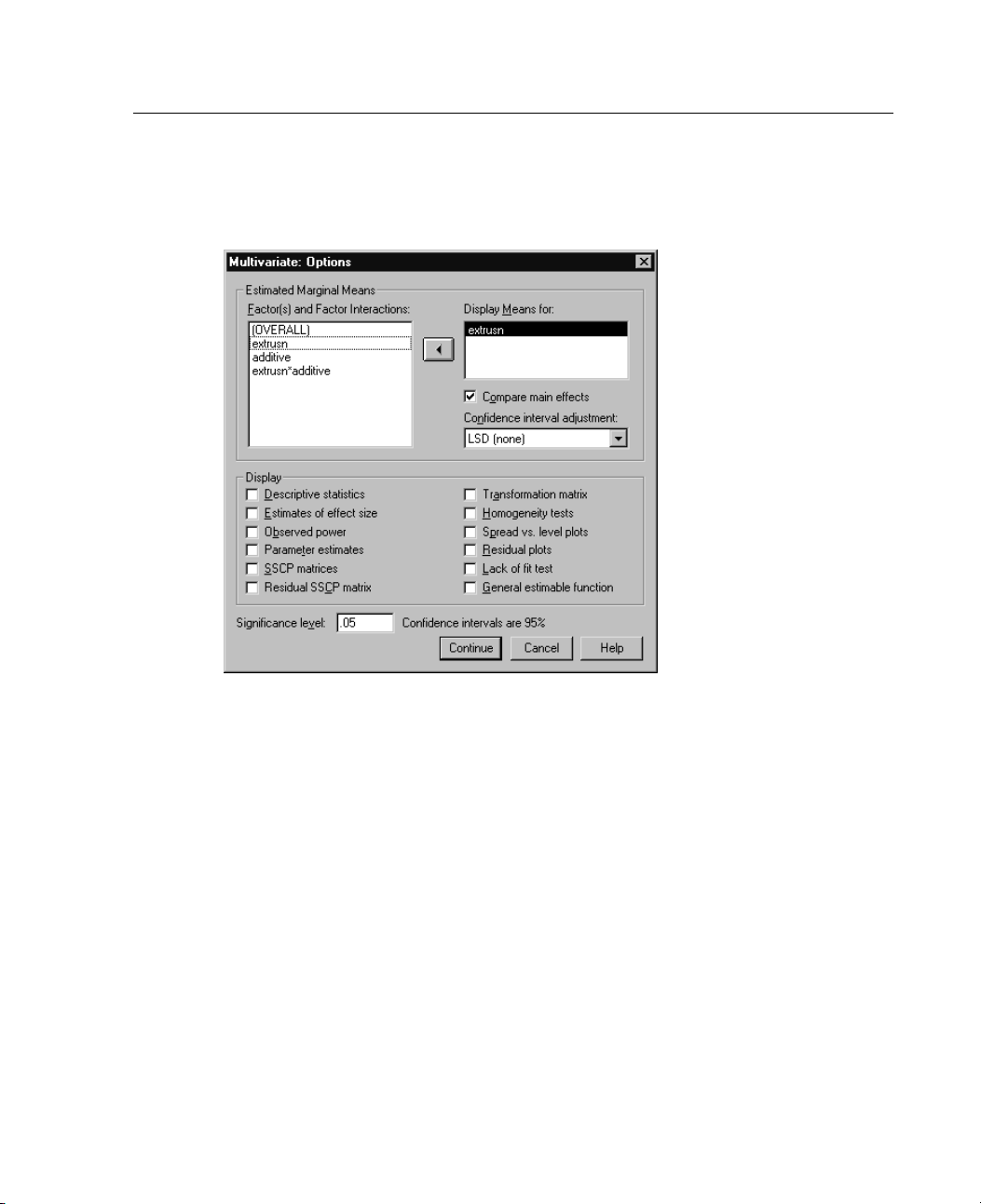
GLM Multivariate Options
Figure 1-8
Multivariat
e Options dialog box
GLM Multivaria
te Analysis
Optional statistics are available from this dialog box. Statistics are calculated u sing
a fixed-effects model.
ted Marginal Means.
Estima
Select the factors and interactions for which you want
estimates of the population marginal means in the cells. These means are adjusted
for the covariates, if any. Interactions are available only if you have specified a
mmodel.
custo
Comp
aremaineffects.
Provides uncorrected pairwise comparisons among
estimated marginal means for any main effect in the model, for both between- and
within-subjects factors. This item is available only if main effects are selected
the Display Means For list.
under
Conf
idence interval adjustment.
Select least significant difference (LSD),
Bonferroni, or Sidak adjustment to the confidence intervals and significance.
This item is available only if
Compare main effects is selected.
Page 24
14
Chapter 1
Display. Select Descriptive statistics to produce observed means, standard deviations,
and counts for all of the dependent variables in all cells. Estimates of effect size gives a
partial eta
-squared value for each effect and each parameter estimate. The eta-squared
statistic describes the proportion of total variability attributable to a factor. Select
Observed power to obtain the power of the test when the alternative hypothesis is set
basedonth
e observed value. Select
Parameter estimates to produce the parameter
estimates, standard errors, t tests, confidence intervals, and the observed power for
each test. You can display the hypothesis and error SSCP matrices and the Residual
plus Bartlett's test of sphericity of the residual covariance matrix.
SSCP matri
Homogeneity tests produces the Levene test of the homogeneity of variance for
x
each dependent variable across all level combinations of the between-subjects factors,
for betwe
en-subjects factors only. Also, homogeneity tests include Box's M test
of the homogeneity of the covariance matrices of the dependent variables across
all level combinations of the between-subjects factors. The spread-versus-level
and resi
This item is disabled if there are no factors. Select
dual plots options are useful for checking assumptions about the data.
Residual plots to produce an
observed-by-predicted-by-standardized residuals plot for each dependent variable.
These pl
Lack of fit test to check if the relationship between the dependent variable and the
ots are useful for investigating the assumption of equal variance. Select
independent variables can be adequately described by the model. General estimable
allows you to construct custom hypothesis tests based on the general
on
functi
estimable function. Rows in any contrast coefficient matrix are linear combinations
of the general estimable function.
GLM C
Signif
icance level.
You might want to adjust the significance level used in post
hoc tests and the confidence level used for constructing confidence intervals. The
specified value is also used to calculate the observed power for the test. When
ecify a significance level, the associated level of the confidence intervals
you sp
is displayed in the dialog box.
ommand Additional Features
e features may apply to univariate, multivariate, or repeated measures analysis.
Thes
The SPSS command language also allows you to:
Specify nested effects in the design (using the DESIGN subcommand).
Page 25
15
GLM Multivaria
Specify tests of effects versus a linear combination of effects or a value (using the
TEST subcom
Specify mul
Include use
Specify EPS
Construct a
MMATRIX,orKMATRIX subcommands).
For deviation or simple contrasts, specify an intermediate reference category
(using the
Specify metrics for polynomial contrasts (using the CONTRAST subcommand).
Specify error terms for post hoc comparisons (using the POSTHOC subcommand).
Compute estimated marginal means for any factor or factor interaction among the
factors in t
Specify na
Construct a
Construct a
ANOVA table (using the
Save the design matrix to a new data file (using the OUTFILE subcommand).
mand).
tiple contrasts (using the
r-missing values (using the
criteria (using the
CONTRAST subcommand).
MISSING subcommand).
CRITERIA subcommand).
custom L matrix, M matrix, or K matrix (using the
CONTRAST subcommand).
he factor list (using the
mes for temporary variables (using the
correlation matrix data file (using the
EMMEANS subcommand).
SAVE subcommand).
OUTFILE subcommand).
matrix data file that contains statistics from the between-subjects
OUTFILE subcommand).
te Analysis
LMATRIX,
See the SPSS
Command Syntax Reference for complete syntax information.
Page 26
Page 27
Chapter
2
GLM Repeated
The GLM Repeated Measures procedure provides analysis of variance when the same
measurement is made several times on each subject or case. If between-subjects
factors are specified, they divide the population into groups. Using this general
linear model procedure, you can test null hypotheses about the effects of both
the between-subjects factors and the within-subjects factors. You can investigate
interactions between factors as well as the effects of individual factors. In addition,
the effects of constant covariates and covariate interactions with the between-subjects
factors can be included.
In a doubly multivariate repeated measures design, the dependent variables
represent measurements of more than one variable for the different levels of the
within-subjects factors. For example, you could have measured both pulse and
respiration at three different times on each subject.
The GLM Repeated Measures procedure p rovides both univariate and multivariate
analyses for the repeated measures data. Both balanced and unbalanced models
can be tested. A design is balanced if each cell in the model contains the same
number of cases. In a multivariate model, the sums of squares due to the effects in
the model and error sums of squares are in matrix form rather than the scalar form
foundinunivariateanalysis.Thesematrices are called SSCP (sums-of-squares and
cross-products) matrices. In addition to testing hypotheses, GLM Repeated Measures
produces estimates of parameters.
Commonly used aprioricontrasts are available to perform hypothesis testing on
between-subjects factors. Additionally, after an overall F test has shown significance,
you can use post hoc tests to evaluate differences among specific means. Estimated
marginal means give estimates of predicted mean values for the cells in the model,
and profile plots (interaction plots) of these means allow you to visualize some of
the relationships easily.
Measures
17
Page 28
18
Chapter 2
Residuals, predicted values, Cook's distance, and leverage values can be saved as
new variables in your data file for checking assumptions. Also available are a residual
SSCP matrix
residuals, a residual covariance matrix, which is the residual SSCP matrix divided by
the degrees of freedom of the residuals, and the residual correlation matrix, which is
the standa
WLS Weight allows you to specify a variable used to give observations different
weights for a weighted least-squares (WLS) analysis, perhaps to compensate for
different
Example. Twelve students are assigned to a high- or low-anxiety group based on their
scores on an anxiety-rating test. The anxiety rating is called a between-subjects factor
because it
a learning task, and the number of errors for each trial is recorded. The errors for each
trial are recorded in separate variables, and a within-subjects factor (trial) is defined
with four
trial-by-anxiety interaction is not significant.
Methods. Type I, Type II, Type III, and Type IV sums of squares can be used to
evaluat
, which is a square matrix of sums of squares and cross-products of
rdized form of the residual covariance matrix.
precision of measurement.
divides the subjects into groups. The students are each given four trials on
levels for the four trials. The trial effect is found to be significant, while the
e different hypotheses. Type III is the default.
GLM Re
Statistics. Post hoc range tests and multiple comparisons (for between-subjects
factors): least significant difference, Bonferroni, Sidak, Scheffé,
Ryan-Ei
Student-Newman-Keuls, Tukey's honestly significant difference, Tukey's-b,Duncan,
Hochberg's GT2, Gabriel, Waller Duncan t test, Dunnett (one-sided and two-sided),
Tamhan
observed means, standard deviations, and counts for all of the dependent variables
in all cells; the Levene test for homogeneity of variance; Box's M; and Mauchly's
test o
Plots. Spread-versus-level, residual, and profile (interaction).
not-Gabriel-Welsch multiple F, Ryan-Einot-Gabriel-Welsch multiple range,
e's T2, Dunnett's T3, Games-Howell, and Dunnett's C. Descriptive statistics:
fsphericity.
peated Measures Data Considerations
The dependent variables should be quantitative. Between-subjects factors divide
Data.
the sample into discrete subgroups, such as male and female. These factors are
categorical and can have numeric values or string values of up to eight characters.
in-subjects factors are defined in the Repeated Measures Define Factor(s)
With
Page 29
19
GLM Repeated Me
asures
dialog box. Covariates are quantitative variables that are related to the dependent
variable. For a repeated measures analysis, these should remain constant at each level
of a within-
subjects variable.
The data file should contain a set of variables for each group of measurements on
the subjects. The set has one variable for each repetition of the measurement within
the group. A
within-subjects factor is defined for the group with the number of levels
equal to the number of repetitions. For example, measurements of weight could be
taken on different days. If measurements of the same property were taken on five
days, the w
ithin-subjects factor could be specified as day with five levels.
For multiple within-subjects factors, the number of measurements for each subject
is equal to the product of the number of levels of each factor. For example, if
measureme
nts were taken at three different times each day for four days, the total
number of measurements is 12 for each subject. The within-subjects factors could be
specified as day(4) and time(3).
ons.
Assumpti
A repeated measures analysis can be approached in two ways, univariate
and multivariate.
The univariate approach (also known as the split-plot or mixed-model approach)
consider
s the dependent variables as responses to the levels of within-subjects
factors. The measurements on a subject should be a sample from a multivariate
normal distribution, and the variance-covariance matrices are the same across the
cells fo
rmed by the between-subjects effects. Certain assumptions are made on the
variance-covariance matrix of the dependent variables. The validity of the F statistic
used in the univariate approach can be assured i f the variance-covariance matrix is
ar in form (Huynh and Mandeville, 1979).
circul
To test this assumption, Mauchly's test of sphericity can be used, which performs
a test of sphericity on the variance-cova riance matrix of an orthonormalized
ormed dependent variable. Mauchly's test is automatically displayed for a
transf
repeated measures analysis. For small sample sizes, this test is not very powerful. For
large sample sizes, the test may be significant even when the impact of the departure
results is small. If the significance of the test is large, the hypothesis of
on the
sphericity can be assumed. However, if the significance is small and the sphericity
assumption appears to be violated, an adjustment to the numerator and denominator
es of freedom can be made in order to validate the univariate F statistic. Three
degre
estimates of this adjustment, which is called epsilon, are available in the GLM
Repeated Measures procedure. Both the numerator and denominator degrees of
dom must be multiplied by epsilon, and the significance of the F ratio must be
free
evaluated with the new degrees of freedom.
Page 30
20
Chapter 2
The multivariate approach considers the measurements on a subject to be a sample
from a multivariate normal distribution, and the variance-covariance matrices are the
same across
variance-covariance matrices across the cells are the same, Box's M test can be used.
Related procedures. Use the Explore procedure to examine the data before doing an
analysis of
GLM Univariate or GLM Multivariate. If there are only two measurements for
each subject (for example, pre-test and post-test), and there are no between-subjects
factors, y
the cells formed by the between-subjects effects. To test whether the
variance. If there are not repeated measurements on each subject, use
ou can use the Paired-Samples T Test procedure.
GLM Repeated Measures Define Factors
GLM Repeated Measures analyzes groups of related dependent variables that
represen
define one or more within-subjects factors for use in GLM Repeated Measures. Note
that the order in which you specify within-subjects factors is important. Each factor
constitu
within-subjects factors in this dialog box. Notice that these factors are not existing
variabl
t different measurements of the same attribute. This dialog box lets you
tes a level within the previous factor.
To use Repeated Measures, you must set up your data correctly. You must define
es in your data but rather factors that you define here.
Example. In a weight-loss study, suppose the weights of several people are measured
each week for five weeks. In the data file, each person is a subject or case. The
weights
gender of each person is recorded in another variable. The weights, measured for each
subject repeatedly, can be grouped by defining a within-subjects factor. The factor
could b
weight1, ..., weight5 areusedtoassignthefivelevelsofweek. The variable in the data
file that groups males and females (gender) can be specified as a between-subjects
facto
Measures. If subjects were tested on more than one measure at each time, define the
measures. For example, the pulse and respiration rate could be measured on each
subje
but are defined here. A model with more than one measure is sometimes called a
doubly multivariate repeated measures model.
for the weeks are recorded in the variables weight1, weight2, and so on. The
e called week, defined to have five levels. In the main dialog box, the variables
r to study the differences between males and females.
ct every day for a week. These measures do not exist as variables in the data file
Page 31
21
Defining Fac
E From the me
Analyze
General Linear Model
Repeated Measures...
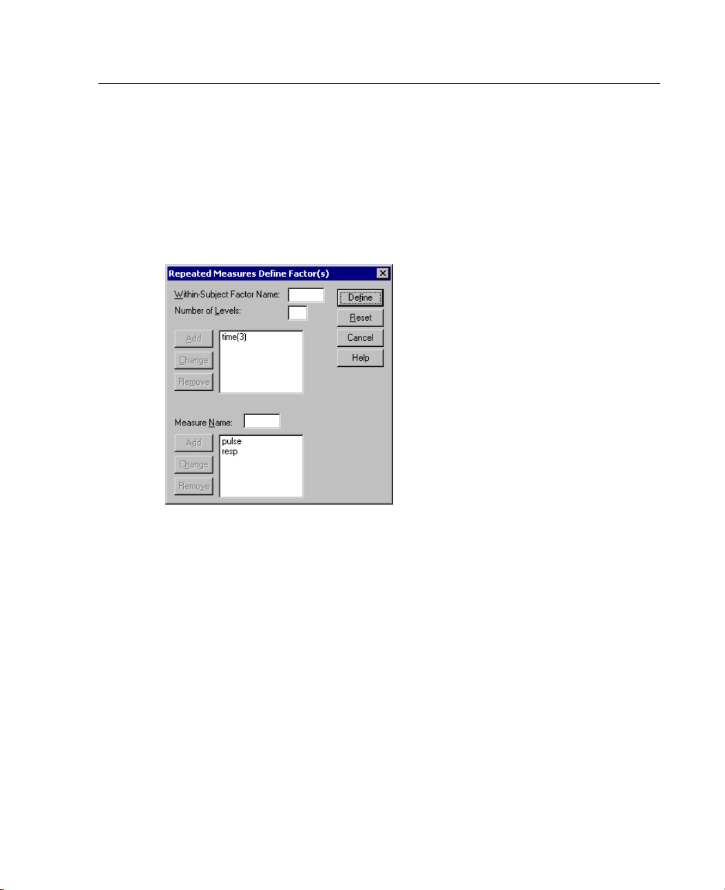
Figure 2-1
Repeated Me
tors for GLM Repeated Measures
nus choose:
asures Define Factor(s) dialog box
GLM Repeated Me
asures
E Typeaw
E Click A
E Repeat
ithin-subject factor name and its number of levels.
.
dd
these steps for each within-subjects factor.
To define measure factors for a doubly multivariate repeated measures design:
E Type the measure name.
E Click Add.
After defining all of your factors and measures:
E Click Define.
Page 32
22
Chapter 2
Obtaining GL
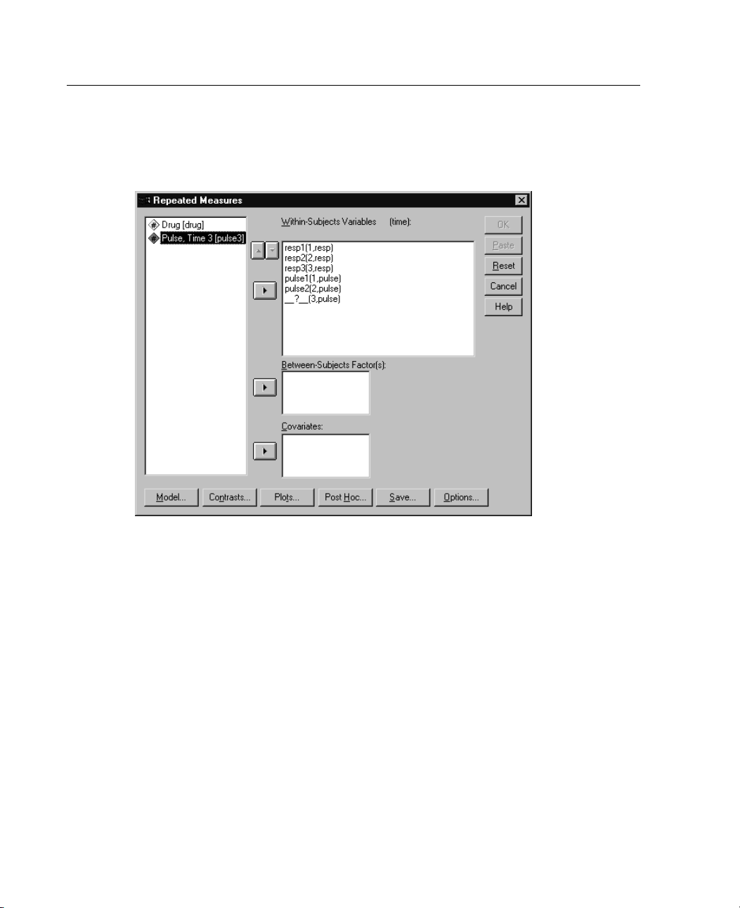
Figure 2-2
Repeated Measures dialog box
E Select a dependent variable that corresponds to each combination of within-subjects
factors (and optionally, measures) on the list.
M Repeated Measures Tables
To change positions of the variables, use the up and down arrows.
To make changes to the within-subjects factors, you can reopen the Repeated
Measures Define Factor(s) dialog box without closing the main dialog box.
Optionally, you can specify between-subjects factor(s) and covariates.
Page 33
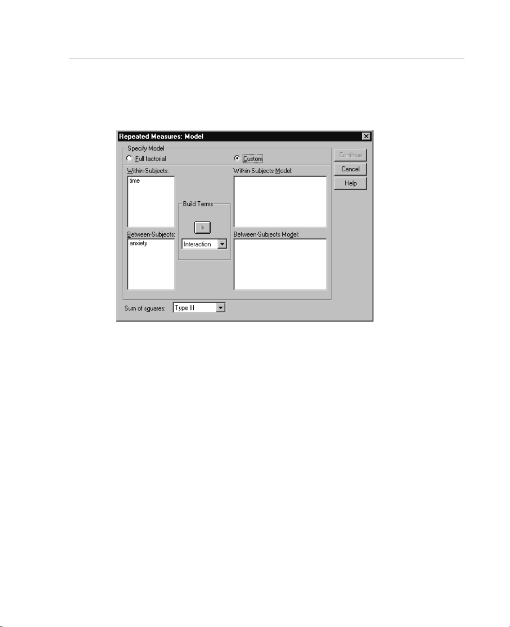
23
GLM Repeated Measures Model
Figure 2-3
Repeated Mea
Specify Model. A full factorial model contains all factor main effects, all covariate
main effects, and all factor-by-factor interactions. It does not contain covariate
interactions. Select
factor-by-covariate interactions. You must indicate all of the terms to be included
in the model.
sures Model dialog box
Custom to specify only a subset of interactions or to specify
GLM Repeated Me
asures
Between-Subjects. The covariates are listed with (C) for covariate.
Model. The model depends on the nature of your data. After selecting Custom,you
can select the within-subjects effects and interactions and the between-subjects effects
and interactions that are of interest in your analysis.
Sum of squares. The method of calculating the sums of squares for the
between-subjects model. For balanced or unbalanced between-subjects models with
no missing cells, the Type III sum-of-squares method is the most commonly used.
Page 34
24
Chapter 2
Build Terms
For the selected factors and covariates:
Interaction. Creates the highest-level interaction term of all selected variables. This is
the default
Main effects. Creates a main-effects term for each variable selected.
All 2-way. Creates all possible two-way interactions of the selected variables.
.
All 3-way. C
All 4-way. Creates all possible four-way interactions of the selected variables.
All 5-way. Creates all possible five-way interactions of the selected variables.
Sums of Squa
For the mode
reates all possible three-way interactions of the selected variables.
res
l, you can choose a type of sum of squares. Type III is the most
commonly used and is the default.
Type I. This method is also known as the hierarchical decomposition of the
sum-of-squ
ares method. Each term is adjusted for only the term that precedes it in the
model. The Type I sum-of-squares method is commonly used for:
A balanced ANOVA model in which any main effects are specified before any
first-ord
er interaction effects, any first-order interaction effects are specified
before any second-order interaction effects, and so on.
A polynomial regression model in which any lower-order terms are specified
before any higher-order terms.
Apurelynestedmodelinwhichthefirst-specifiedeffectisnestedwithinthe
second-sp
ecified effect, t he second-specified effect is nested within the third, and
so on. (This form of nesting can be specified only by using syntax.)
Type II. T
his method calculates the sums of squares of an effect in the model adjusted
for all other “appropriate” effects. An appropriate effect is one that corresponds to all
effects that do not contain the effect being examined. The Type II sum-of-squares
method is
A balanc
Any mode
commonlyusedfor:
ed ANOVA model.
l that has main factor effects only.
Page 35
25
GLM Repeated Me
Any regression model.
A purely nested design. (This form of nesting can be specified by using syntax.)
Type III. This method, the default, calculates the sums of squares of an effect in the
design as the
sums of squares adjusted for any other effects that do not contain
asures
it and orthogonal to any effects (if any) that contain it. The Type III sums of
squares have one major advantage in that they are invariant with respect to the cell
frequencie
saslongasthegeneralformofestimability remains constant. Therefore,
this type is often considered useful for an unbalanced model with no missing
cells. In a factorial design with no missing cells, this method is equivalent to the
Yates' wei
ghted-squares-of-means technique. The Type III sum-of-squares method
is commonly used for:
AnymodelslistedinTypeIandTypeII.
Any balanced or unbalanced model with no empty cells.
Type IV. This method is designed for a situation in which there are missing cells. For
any effect
F in the design, if F is not contained in any other effect, then Type IV =
Type III = Type II. When F is contained in other effects, Type IV distributes the
contrasts being made among the parameters in F to all higher-level effects equitably.
The Type I
Any mode
Any bala
V sum-of-squares method is commonly used for:
ls listed in Type I and Type II.
nced model or unbalanced model with empty cells.
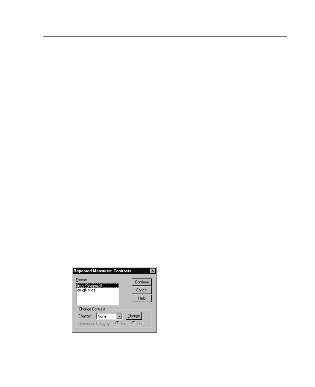
GLM Repeated Measures Contrasts
Figure 2-4
Repeated Measures Contrasts dialog box
Page 36
26
Chapter 2
Contrast Types
Contrasts are used to test for differences among the levels of a between-subjects
factor. You can specify a contrast for each between-subjects factor in the model.
Contrasts r
epresent linear combinations of the parameters.
Hypothesis testing is based on the null hypothesis LBM=0, where L is the contrast
coefficients matrix, B is the parameter vector, and M is the average matrix that
correspond
display t his transformation matrix by selecting
s to the average transformation for the dependent variable. You can
Transformation matrix in the Repeated
Measures Options dialog box. For example, if there are four dependent variables, a
within-su
bjects factor of four levels, and polynomial contrasts (the default) are used
for within-subjects factors, the M matrix will be (0.5 0.5 0.5 0.5)'. When a contrast
is specified, SPSS creates an L matrix such that the columns corresponding to the
between-
subjects factor match the contrast. The remaining columns are adjusted so
that the L matrix is estimable.
A vailable contrasts are deviation, simple, difference, Helmert, repeated, and
polynomi
al. For deviation contrasts and simple contrasts, you can choose whether the
reference category is the last or first category.
Deviation. Compares the mean of each level (except a reference category) to the mean
of all of
Simple. Compares the mean of each level to the mean of a specified level. This
the levels (grand mean). The levels of the factor can be in any order.
type of contrast is useful when there is a control group. You can choose the first or
egory as the reference.
last cat
Difference. Compares the mean of each level (except the first) to the mean of previous
levels. (Sometimes called reverse Helmert contrasts.)
t.
Helmer
Compares the mean of each level of the factor (except the last) to the mean
of subsequent levels.
Repeated. Compares the mean of each level (except the last) to the mean of the
uent level.
subseq
Polynomial. Compares the linear effect, quadratic effect, cubic effect, and so on. The
first degree of freedom contains the linear effect across all categories; the second
degree
of freedom, the quadratic effect; and so on. These contrasts are often used
to estimate polynomial trends.
Page 37
27
GLM Repeated Measures Profile Plots
Figure 2-5
Repeated Mea
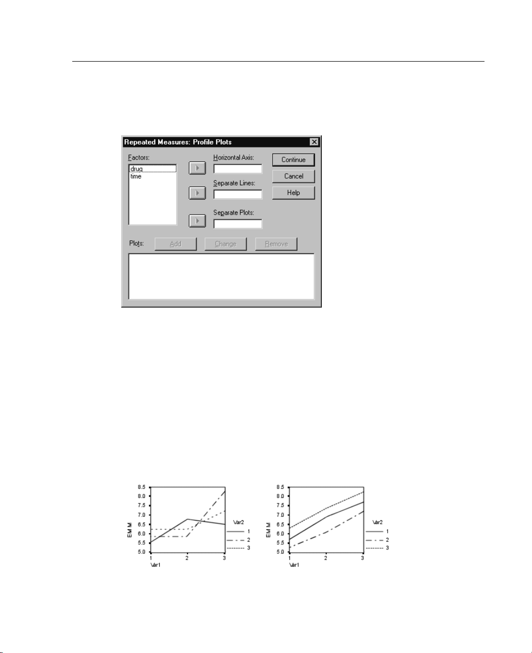
Profile plots (interaction plots) are useful for comparing marginal means in your
model. A profile plot is a line plot in which each point indicates the estimated
marginal mean of a dependent variable (adjusted for any covariates) at one level of a
factor. The levels of a second factor can be used to make separate lines. Each level in
a third factor can be used to create a separate plot. Both between-subjects factors
and within-subjects factors can be used in profile plots.
A profile plot of one factor shows whether the estimated marginal means are
increasing or decreasing across levels. For two or more factors, parallel lines indicate
that there is no interaction between factors, which means that you can investigate the
levels of only one factor. Nonparallel lines indicate an interaction.
sures Profile Plots dialog box
GLM Repeated Me
asures
Figure 2-6
Nonparallel plot (left) and parallel plot (right)
Page 38
28
Chapter 2
After a plot is specified by selecting factors for the horizontal axis and, optionally,
factors for separate lines and separate plots, it must be added to the Plots list.
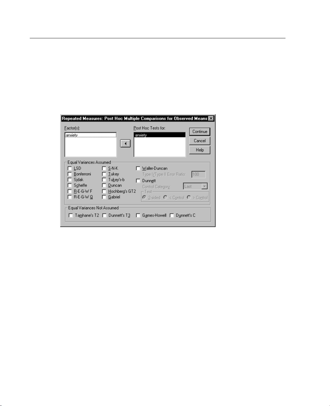
GLM Repeated Measures Post Hoc Multiple Comparisons for Observed Means
Figure 2-7
Post H oc Mul
Post ho
tiple Comparisons for Observed Means dialog box
c multip le comparison tests.
Once you have determined that differences
exist among the means, post hoc range tests and pairwise multiple comparisons
can determine which means differ. These tests are used for fixed between-subjects
s only. They are not available if there are no between-subjects factors. The
factor
post hoc multiple comparison tests are performed for the average across the levels
of the within-subjects factors.
The Bo
nferroni and Tukey's honestly significant difference tests are commonly
used multiple comparison tests. The Bonferroni test, based on Student's t statistic,
adjusts the observed significance level for the fact that multiple comparisons are
Sidak's t test also adjusts the significance level and provides tighter bounds
made.
than the Bonferroni test. Tukey's honestly significant difference test uses the
Studentized range statistic to make all pairwise comparisons between groups and sets
xperimentwise error rate to the error rate for the collection for all pairwise
the e
comparisons. When testing a large number of pairs of means, Tukey's honestly
Page 39
29
GLM Repeated Me
asures
significant difference test is more powerful than the Bonferroni test. For a small
number of pairs, Bonferroni is more powerful.
Hochberg's G
T2 is similar to Tukey's honestly significant difference test, but the
Studentized maximum modulus is used. Usually, Tukey's test is more powerful.
Gabriel's pairwise comparisons test also uses the Studentized maximum modulus
and is gener
ally more powerful than Hochberg's GT2 when the cell sizes are unequal.
Gabriel's test may become liberal when the cell sizes vary greatly.
Dunnett's pairwise multiple comparison t test compares a set of treatments
against a s
ingle control mean. The last category is the default control category.
Alternatively, you can choose the first category. You can also choose a two-sided or
one-sided test. To test that the mean at any level (except the control category) of the
factor is n
ot equal to that of the control category, use a two-sided test. To test whether
the mean at any level of the factor is smaller than that of the control category, select
. Likewise, to test whether the mean at any level of the factor is larger than that
Control
of the con
trol category, select
> Control.
Ryan, Einot, Gabriel, and Welsch (R-E-G-W) developed two multiple step-down
range tests. Multiple step-down procedures first test whether all means are equal.
If all mea
ns are not equal, subsets of means are tested f or equality. R-E-G-W F is
based on an F test and R-E-G-W Q is based on the Studentized range. These tests
are more powerful than Duncan's multiple range test and Student-Newman-Keuls
(which a
re also multiple step-down procedures), but they are not recommended
for unequal cell sizes.
When the variances are unequal, use Tamhane's T2 (conservative pairwise
compar
isons test based on a t test), Dunnett's T3 (pairwise comparison test based
on the Studentized maximum modulus), Games-Howell pairwise comparison
test (sometimes liberal), or Dunnett's C (pairwise comparison test based on the
tized range).
Studen
Duncan's multiple range test, Student-Newman-Keuls (S-N-K), and Tukey's-b
are range tests that rank group means and compute a range value. These tests are
ed as frequently as the tests previously discussed.
not us
The Waller-Duncan t test uses a Bayesian approach. This range test uses the
harmonic mean of the sample size when the sample sizes are unequal.
gnificance level of the Scheffé test is designed to allow all possible linear
The si
combinations of group means to be tested, not just pairwise comparisons available in
this feature. The result is that the Scheffé test is often more conservative than other
, which means that a larger difference between means is required for significance.
tests
<
Page 40
30
Chapter 2
The least significant difference (LSD) pairwise multiple comparison test is
equivalent to multiple individual t tests between all pairs of groups. The disadvantage
of this test
is that no attempt is made to adjust the observed significance level for
multiple comparisons.
Tests displayed. Pairwise comparisons are provided for LSD, Sidak, Bonferroni,
Games and Ho
well, Tamhane's T2 and T3, Dunnett's C, and Dunnett's T3.
Homogeneous subsets for range tests are provided for S-N-K, Tukey's-b,Duncan,
R-E-G-W F, R-E-G-W Q, and Waller. Tukey's honestly significant difference test,
Hochberg'
s GT2, Gabriel's test, and Scheffé's test are both multiple comparison
tests and range tests.
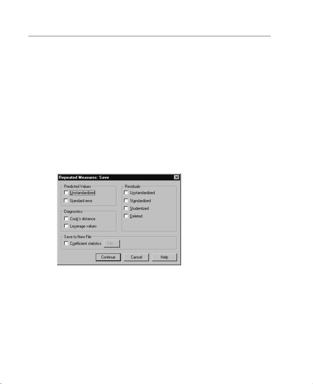
GLM Repea
Figure 2-8
Repeated Measures Save dialog box
You can save values predicted by the model, residuals, and related measures as new
variables in the Data Editor. Many of these variables can be used for examining
assumptions about the data. To save the values for use in another SPSS session, you
must save the current data file.
Predicted Values. The values that the model predicts for each case. Unstandardized
predicted values and the standard errors of the predicted values are available.
ted Measures Save
Page 41
31
GLM Repeated Me
Diagnostics. Measures to identify cases with unusual combinations of values for the
asures
independent variables and cases that may have a large impact on the model. Ava ilable
are Cook's d
Cook's Dis
istance and uncentered leverage values.
tance.
A measure of how much the residuals of all cases would
change if a particular case were excluded from the calculation of the regression
coefficients. A large Cook's D indicates that excluding a case from computation
of the regr
Leverage V
Residuals. An unstandardized residual is the actual value of the dependent variable
ession statistics, changes the coefficients substantially.
alue.
The relative influence of each observation on the model's fit.
minus the value predicted by the model. Standardized, Studentized, and deleted
residuals
Unstanda
are also available.
rdized Residuals.
The difference between an observed value and the
valuepredictedbythemodel.
Standardized. The residual divided by an estimate of its standard error.
Standardized residuals are also known as Pearson residuals.
Studentized Residual. The residual divided by an estimate of its standard deviation
that varie
s from case to case, depending on the distance of each case's values on
the independent variables from the means of the independent variables.
Deleted Residual. The residual for a case when that case is excluded from the
calculation of the regression coefficients. It is the difference between the value of
the depen
dent variable and the adjusted predicted value.
Save to New File. Writes an SPSS data file containing a variance-covariance matrix of
the parameter estimates in the model. Also, for each dependent variable, there will
bearowo
f parameter estimates, a row of significance values for the t statistics
corresponding to the parameter estimates, and a row of residual degrees of freedom.
For a multivariate model, there are similar rows for each dependent variable. You can
use this
matrix file in other procedures that read an SPSS matrix file.
Page 42
32
Chapter 2
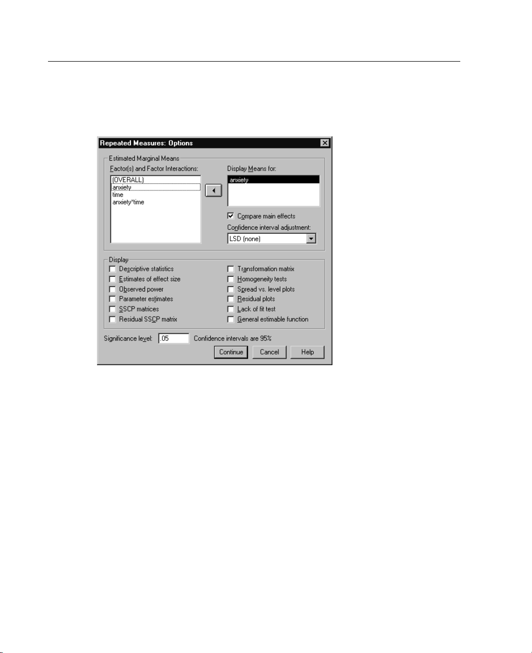
GLM Repeated Measures Options
Figure 2-9
Repeated Mea
sures Options dialog box
Optional statistics are available from this dialog box. Statistics are calculated u sing
-effects model.
afixed
Estimated M arginal Means. Select the factors and interactions for which you want
estimates of the population marginal means in the cells. These means are adjusted
e covariates, if any. Both within-subjects and between-subjects factors can
for th
be selected.
Compare main effects. Provides uncorrected pairwise comparisons among
ated marginal means for any main effect in the model, for both between- and
estim
within-subjects factors. This item is available only if main effects are selected
under the Display Means For list.
Confidence interval adjustment. Select least significant difference (LSD),
rroni, or Sidak adjustment to the confidence intervals and significance.
Bonfe
This item is available only if
Compare main effects is selected.
Page 43
33
GLM Repeated Me
Display. Select Descriptive statistics to produce observed means, standard deviations,
asures
and counts for all of the dependent variables in all cells. Estimates of effect size gives a
partial eta
-squared value for each effect and each parameter estimate. The eta-squared
statistic describes the proportion of total variability attributable to a factor. Select
Observed power to obtain the power of the test when the alternative hypothesis is set
basedonth
e observed value. Select
Parameter estimates to produce the parameter
estimates, standard errors, t tests, confidence intervals, and the observed power for
each test. You can display the hypothesis and error SSCP matrices and the Residual
plus Bartlett's test of sphericity of the residual covariance matrix.
SSCP matri
Homogeneity tests produces the Levene test of the homogeneity of variance for
x
each dependent variable across all level combinations of the between-subjects factors,
for betwe
en-subjects factors only. Also, homogeneity tests include Box's M test
of the homogeneity of the covariance matrices of the dependent variables across
all level combinations of the between-subjects factors. The spread-versus-level
and resi
This item is disabled if there are no factors. Select
dual plots options are useful for checking assumptions about the data.
Residual plots to produce an
observed-by-predicted-by-standardized residuals plot for each dependent variable.
These pl
Lack of fit test to check if the relationship between the dependent variable and the
ots are useful for investigating the assumption of equal variance. Select
independent variables can be adequately described by the model. General estimable
allows you to construct custom hypothesis tests based on the general
on
functi
estimable function. Rows in any contrast coefficient matrix are linear combinations
of the general estimable function.
GLM C
Signif
icance level.
You might want to adjust the significance level used in post
hoc tests and the confidence level used for constructing confidence intervals. The
specified value is also used to calculate the observed power for the test. When
ecify a significance level, the associated level of the confidence intervals
you sp
is displayed in the dialog box.
ommand Additional Features
e features may apply to univariate, multivariate, or repeated measures analysis.
Thes
The SPSS command language also allows you to:
Specify nested effects in the design (using the DESIGN subcommand).
Page 44
34
Chapter 2
Specify tests of effects versus a linear combination of effects or a value (using the
TEST subcom
Specify mul
Include use
Specify EPS
Construct a
MMATRIX,andKMATRIX subcommands).
For deviation or simple contrasts, specify an intermediate reference category
(using the
Specify metrics for polynomial contrasts (using the CONTRAST subcommand).
Specify error terms for post hoc comparisons (using the POSTHOC subcommand).
Compute estimated marginal means for any factor or factor interaction among the
factors in t
Specify na
Construct a
Construct a
ANOVA table (using the
Save the design matrix to a new data file (using the OUTFILE subcommand).
mand).
tiple contrasts (using the
r-missing values (using the
criteria (using the
custom L matrix, M matrix, or K matrix (using the
CONTRAST subcommand).
he factor list (using the
mes for temporary variables (using the
correlation matrix data file (using the
CONTRAST subcommand).
MISSING subcommand).
CRITERIA subcommand).
LMATRIX,
EMMEANS subcommand).
SAVE subcommand).
OUTFILE subcommand).
matrix data file that contains statistics from the between-subjects
OUTFILE subcommand).
See the SPSS
Command Syntax Reference for complete syntax information.
Page 45
Chapter
3
Variance Com
The Variance Components procedure, for mixed-effects models, estimates the
contribution of each random effect to the variance of the dependent variable. This
procedure is particularly interesting for analysis of mixed models such as split plot,
univariate repeated measures, and random block designs. By calculating variance
components, you can determine where to focus attention in order to reduce the
variance.
Four different methods are available for estimating the variance components:
minimum norm quadratic unbiased estimator (MINQUE), analysis of variance
(ANOVA), maximum likelihood (ML), and restricted maximum likelihood (REML).
Various specifications are available for the different methods.
Default output for all methods includes variance component estimates. If the ML
method or the REML method is used, an asymptotic covariance matrix table is also
displayed. Other available output includes an ANOVA table and expected mean
squares for the ANOVA method, and an iteration history for the ML and REML
methods. The Variance Components procedure is fully compatible with the GLM
Univariate procedure.
WLS Weight allows you to specify a variable used to give observations different
weights for a weighted analysis, perhaps to compensate for different precision
of measurement.
ponents Analysis
Example. At an agriculture school, weight gains for pigs in six different litters are
measured after one month. The litter variable is a random factor with six levels. (The
six litters studied are a random sample from a large population of pig litters.) The
investigator finds out that the variance in weight gain is attributable to the difference
in litters much more than to the difference in pigs within a litter.
35
Page 46
36
Chapter 3
Variance Com
Data. The de
numeric values or string values of up to eight characters. At least one of the factors
must be random. That is, the levels of the factor must be a random sample of possible
levels. Cov
Assumptions. All methods assume that model parameters of a random effect have zero
means and finite constant variances and are mutually uncorrelated. Model parameters
from diffe
The residual term also has a zero mean and finite constant variance. It is
uncorrelated with model parameters of any random effect. Residual terms from
different
Based on these assumptions, observations from the same level of a random factor
are correlated. This fact distinguishes a variance component model from a general
linear mo
ANOVA and MINQUE do not require normality assumptions. They are both
robust to moderate departures from the normality assumption.
ML and REML
distributed.
Related procedures. Use the Explore procedure to examine the data before doing
variance
Multivariate, and GLM Repeated Measures.
ponents Data Considerations
pendent variable is quantitative. Factors are categorical. They can have
ariates are quantitative variables that are related to the dependent variable.
rent random effects are also uncorrelated.
observations are assumed to be uncorrelated.
del.
require the model parameter and the residual term to be normally
components analysis. For hypothesis testing, use GLM Univariate, GLM
Obtaini
E From th
ng Variance Components Tables
e menus choose:
Analyze
General Linear Model
Variance Components...
Page 47
37
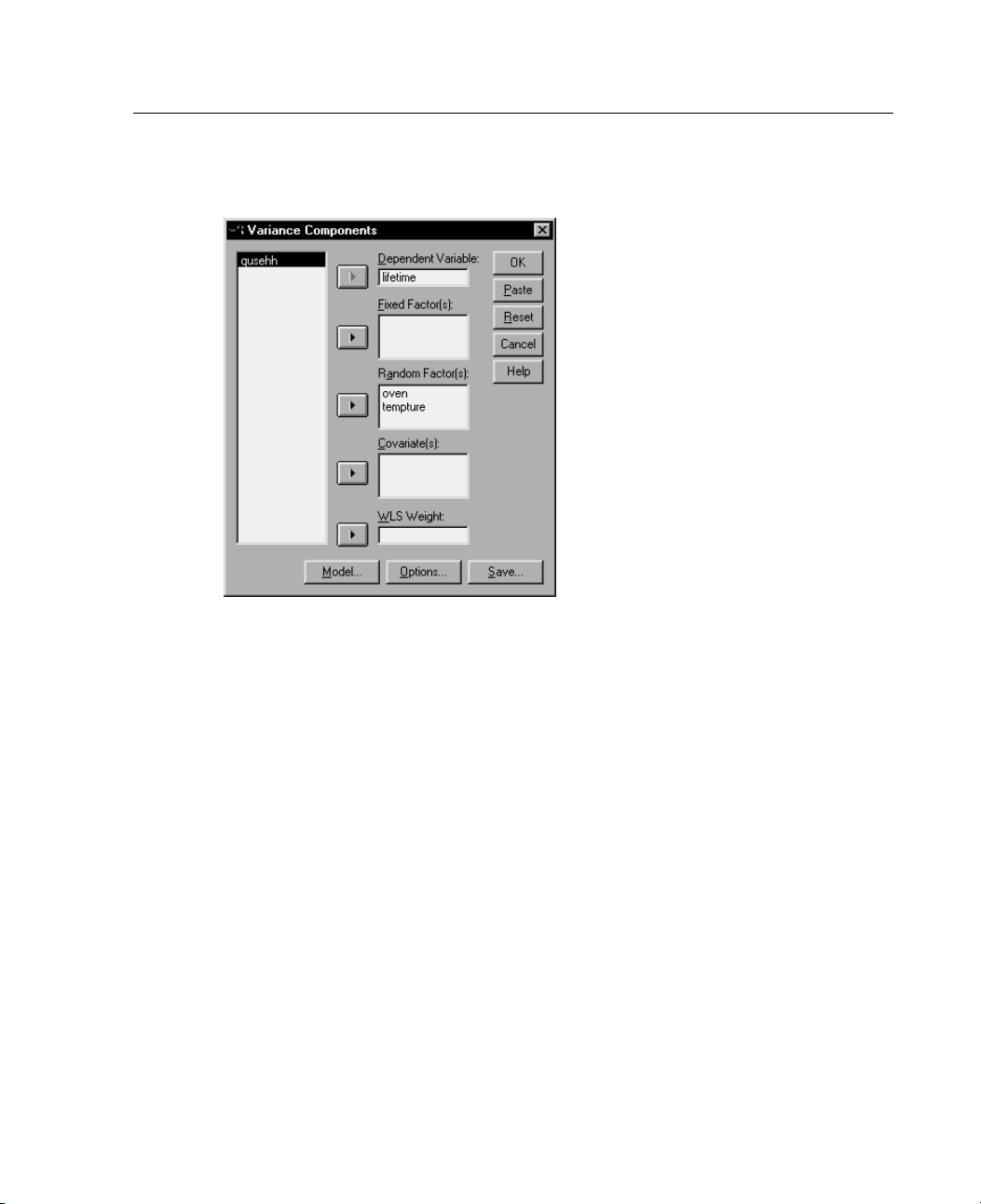
Figure 3-1
Variance Components dialog box
E Select a dependent variable.
Variance Compo
nents Analysis
E Select variables for Fixed Factor(s), Random Factor(s), and Covariate(s), as
appropriate for your data. For specifying a weight variable, use WLS Weight.
Page 48
38
Chapter 3
Variance Components Model
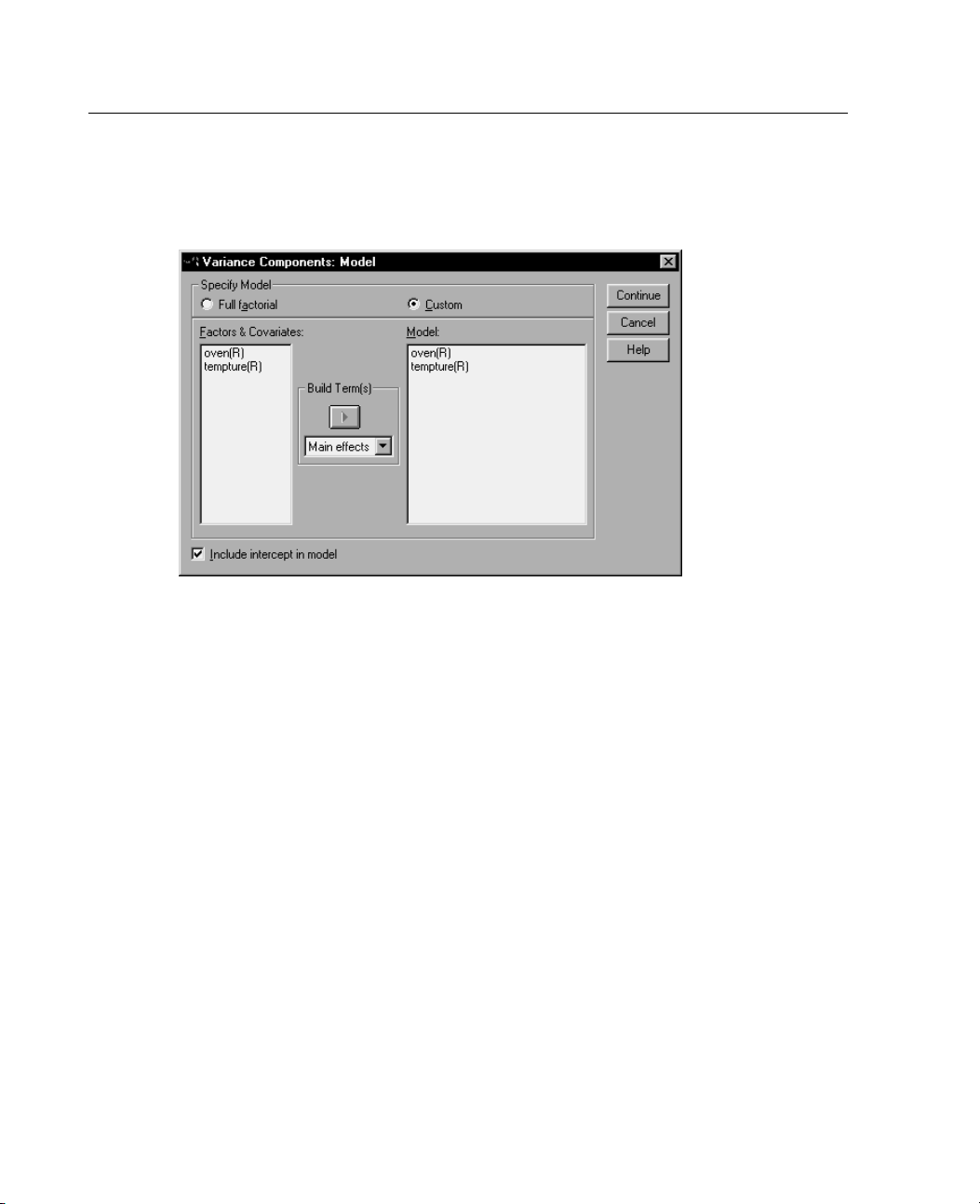
Figure 3-2
Variance Com
Specify Model. A full factorial model contains all factor main effects, all covariate
ponents Model dialog box
main effects, and all factor-by-factor interactions. It does not contain covariate
interactions. Select Custom to specify only a subset of interactions or to specify
factor-by-covariate interactions. You must indicate all of the terms to be included
in the model.
Factors and Covariates. The factors and covariates are listed with (F) for a fixed factor,
(R) for a random factor, and (C) for a covariate.
Model. The model depends on the nature of your data. After selecting Custom,you
can select the main effects and interactions that are of interest in your analysis. The
model must contain a random factor.
Include intercept in model. Usually the intercept is included in the model. If you can
assume that the data pass through the origin, you can exclude the intercept.
Page 49
39
Build Terms
For the selected factors and covariates:
Interaction. Creates the highest-level interaction term of all selected variables. This is
the default
Main effects. Creates a main-effects term for each variable selected.
All 2-way. Creates all possible two-way interactions of the selected variables.
All 3-way. C
All 4-way. Creates all possible four-way interactions of the selected variables.
All 5-way. Creates all possible five-way interactions of the selected variables.
.
reates all possible three-way interactions of the selected variables.
Variance Components Options
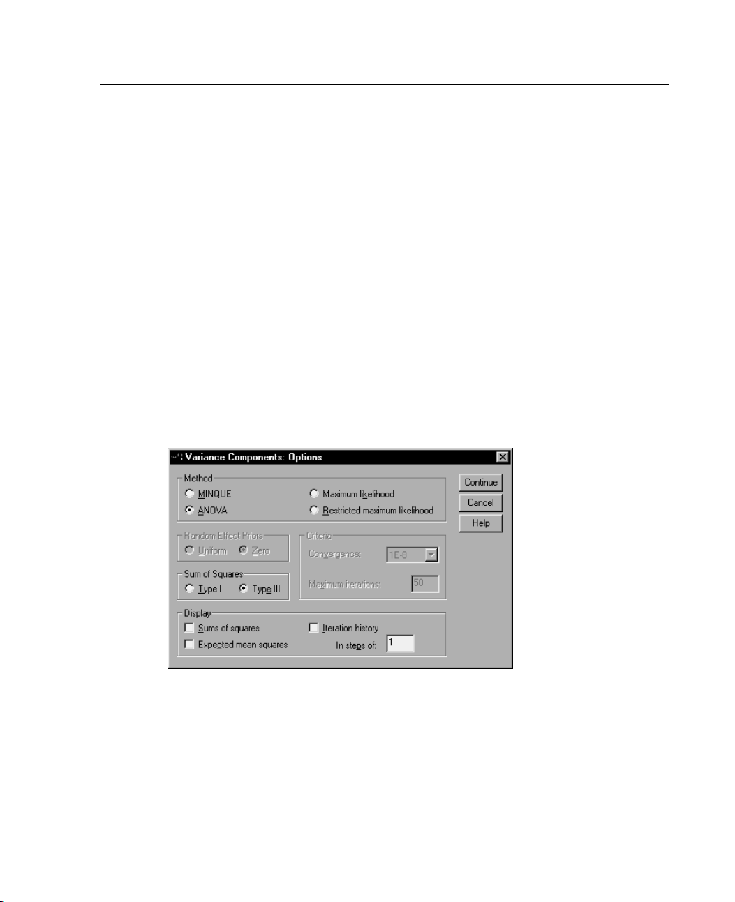
Figure 3-3
Variance Co
mponents Options dialog box
Variance Compo
nents Analysis
Method. You can choose one of four methods to estimate the variance components.
MINQUE (minimum norm quadratic unbiased estimator) produces estimates that
are invariant with respect to the fixed effects. If the data are normally distributed
and the e
stimates are correct, this method produces the least variance among all
unbiased estimators. You can choose a method for random-effect prior weights.
Page 50
40
Chapter 3
ANOVA
IorTypeIII
(analysis of variance) computes unbiased estimates using either the Type
sums of squares for each effect. The ANOVA method sometimes
produces negative variance estimates, which can indicate an incorrect model, an
inappropriate estimation method, or a need for more data.
Maximum likelihood (ML) produces estimates that would be most consistent with
the data act
ually observed, using iterations. These estimates can be biased. This
method is asymptotically normal. ML and REML estimates are invariant under
translation. This method does not take into account the degrees of freedom used
to estimat
Restrict
e the fixed effects.
ed maximum likelihood
(REML) estimates reduce the ANOVA estimates
for many (if not all) cases of balanced data. Because this method is adjusted for
the fixed effects, it should have smaller standard errors than the ML method.
This meth
od takes into account the degrees of freedom used to estimate the
fixed effects.
Random-E
ffect Priors.
Uniform implies that all random effects and the residual term
have an equal impact on the observations. The Zero scheme is equivalent to assuming
zero random-effect variances. Available only for the MINQUE method.
ares.
Sum of Squ
Type I sums of squares are used for the hierarchical model, which
is often used in variance component literature. If you choose Type III, the default in
GLM, the variance estimates can be used in GLM Univariate for hypothesis testing
with Typ
e III sums of squares. Available only for the ANOVA method.
Criteria. You can specify the convergence criterion and the maximum number of
iterations. Available only for the ML or REML methods.
.
Display
For the ANOVA method, you can choose to display sums of squares and
expected mean squares. If you selected Maximum likelihood or Restricted maximum
likelihood
Sum of S
For the
, you can display a history of the iterations.
quares (Variance Components)
model, you can choose a type of sum of squares. Type III is the most
commonly used and is the default.
Page 51
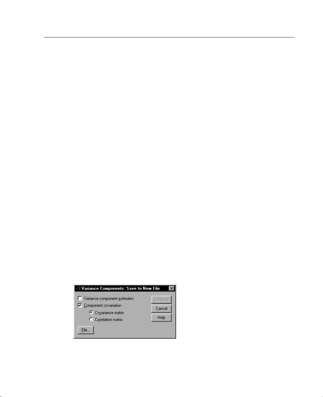
41
Variance Compo
Type I. This method is also known as the hierarchical decomposition of the
nents Analysis
sum-of-squares method. Each term is adjusted for only the term that precedes it in the
model. The T
A balanced
ype I sum-of-squares method is commonly used for:
ANOVA model in which any main effects are specified before any
first-order interaction effects, any first-order interaction effects are specified
before any second-order interaction effects, and so on.
A polynomial regression model in which any lower-order terms are specified
before any h
Apurelyne
igher-order terms.
sted model in which the first-specified effect is nested within the
second-specified effect, the second-specified effect is nested within the third, and
so on. (This form of nesting can be specified only by using syntax.)
Type III. This method, the default, calculates the sums of squares of an effect in the
design as t
he sums of squares adjusted for any other effects that do not contain
it and orthogonal to any effects (if any) that contain it. The Type III sums of
squares have one major advantage in that they are invariant with respect to the cell
frequenc
iesaslongasthegeneralformofestimability remains constant. Therefore,
this type is often considered useful for an unbalanced model with no missing
cells. In a factorial design with no missing cells, this method is equivalent to the
Yates' w
eighted-squares-of-means technique. The Type III sum-of-squares method
is commonly used for:
Any models listed in Type I.
Any balanced or unbalanced model with no empty cells.
Varianc
e Components Save to a File
Figure 3-4
Variance Components Save to New File dialog box
Page 52
42
Chapter 3
You can save some results of this procedure to a new SPSS data file.
Variance component estimates. Saves estimates of the variance components and
estimate la
bels to a data file. These can be used in calculating more statistics or in
further analysis in the GLM procedures. For example, you can use them to calculate
confidence intervals or test hypotheses.
Component c
ovariation.
Saves a variance-covariance matrix or a correlation matrix
to a data file. Available only if Maximum likelihood or Restricted maximum likelihood
has been specified.
e.
Save to Fil
Allows you to specify a filename for the file containing the variance
component estimates and/or the matrix.
You can use the
MATRIX command to extract the data you need from the new file and
then compute confidence intervals or perform tests.
VARCOMP Command Additional Features
The SPSS command language also allows you to:
Specify nested effects in the design (using the DESIGN subcommand).
Include user-missing values (using the MISSING subcommand).
Specify EPS criteria (using the CRITERIA subcommand).
See the SPSS Command Syntax Reference for complete syntax information.
Page 53
Chapter
4
Linear Mixed
The Linear Mixed Models procedure expands the general linear model so that the
data are per
model, therefore, provides the flexibility of modeling not only the means of the data
but their variances and covariances as well.
The Linear
that can be formulated as mixed linear models. Such models include multilevel
models, h ierarchical linear models, and random coefficient models.
Example. A
customer spending. Taking a random sample of their regular customers, they follow
the spending of each customer for 10 weeks. In each week, a different coupon
is mailed
of different coupons on spending while adjusting for correlation due to repeated
observations on each subject over the 10 weeks.
Methods.
estimation.
mitted to exhibit correlated and non-constant variability. The mixed linear
Mixed Models procedure is also a flexible tool for fitting other models
grocery store chain is interested in the effects of various coupons on
to the customers. Linear Mixed Models is used to estimate the effect
Maximum likelihood (ML) and restricted maximum likelihood (REML)
Models
Statistics. Descriptive statistics: sample sizes, means, and standard deviations of
the depe
factors. Factor-level information: sorted values of the levels of each factor and their
frequencies. Also, parameter estimates and confidence intervals for fixed effects,
Wald te
and Type III sums of squares can be used to evaluate different hypotheses. Type
III is the default.
ndent variable and covariates for each distinct level combination of the
sts and confidence intervals for parameters of covariance matrices. Type I
43
Page 54
44
Chapter 4
Linear Mixed
Data. The de
and can have numeric values or string values. Covariates and the weight variable
should be quantitative. Subjects and repeated variables may be of any type.
Assumption
fixed factors, random factors, and covariates. The fixed effects model the mean
of the dependent variable. The random effects model the covariance structure of
the depend
each other, and separate covariance matrices will be computed for each; however,
model terms specified on the same random effect can be correlated. The repeated
measures
is also assumed to come from a normal distribution.
Related procedures. UsetheExploreproceduretoexaminethedatabeforerunningan
analysis
can alternatively use the GLM Univariate or GLM R epeated Measures procedure.
You can alternatively use the Variance Components Analysis procedure if the random
have a variance components covariance structure and there are no repeated
effects
measures.
Linear M
ixed Models Select Subjects/Repeated Variables
Models Data Considerations
pendent variable should be quantitative. Factors should be categorical
s.
The dependent variable is assumed to be linearly related to the
ent variable. Multiple random effects are considered independent of
model the covariance structure of the residuals. The dependent variable
. If you do not suspect there to be correlated or nonconstant variability, you
This dia
observations and to choose a covariance structure for the residuals.
Subjects. A subject is an observational unit that can be considered independent of
other s
study can be considered independent of the readings from other patients. Defining
subjects becomes particularly important when there are repeated measurements
per su
example, you might expect that blood pressure readings from a single patient during
consecutive visits to the doctor are correlated.
for example, you can specify Gender and Age category as subject variables to model
the belief that malesovertheageof65are similar to each other but independent of
male
log box allows you to select variables that define subjects and repeated
ubjects. For example, the blood pressure readings from a patient in a medical
bject and you want to model the correlation between these observations. For
cts can also be defined by the factor-level combination of multiple variables;
Subje
s under 65 and females.
Page 55
45
Linear Mixed Mo
dels
All of the variables specified in the Subjects list are used to define subjects for
the residual covariance structure. You can use some or all of the variables to define
subjects fo
r the random-effects covariance structure.
Repeated. The variables specified in this list are used to identify repeated observations.
For example, a single variable Week might identify the 10 weeks of observations
in a medical
study, or Month and Day might be used together to identify daily
observations over the course of a year.
Repeated Covariance type. This specifies the covariance structure for the residuals.
The availa
Ante-Dep
AR(1)
AR(1): He
ARMA(1,1
Compound S
Compound S
Compound S
Diagonal
Factor Ana
Factor Ana
Huynh-Fel
Scaled Ide
Toeplitz
Toeplitz:
Unstructu
Unstructu
ble structures are as follows:
endence: First Order
terogeneous
)
ymmetry
ymmetry: Correlation Metric
ymmetry: Heterogeneous
lytic: First Order
lytic: First Order, Heterogeneous
dt
ntity
Heterogeneous
red
red: Correlations
For more information, see “Covariance Structures” in Appendix B on page 125.
Page 56
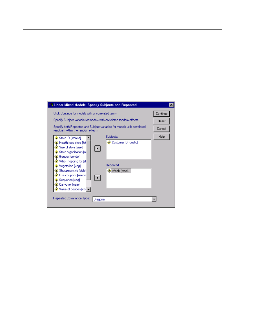
46
Chapter 4
Selecting Su
Models
E From the menus choose:
Analyze
Mixed Models
Linear...
Figure 4-1
Linear Mixed Mod el s Spe cify S ubj ects/Repeated Variables dialog box
bjects/Repeated Variables for Linear Mixed
E Optionally, select one or more subjects variables.
E Optionally, select one or more repeated variables.
E Optionally, select a residual covariance structure.
E Click Continue.
Page 57
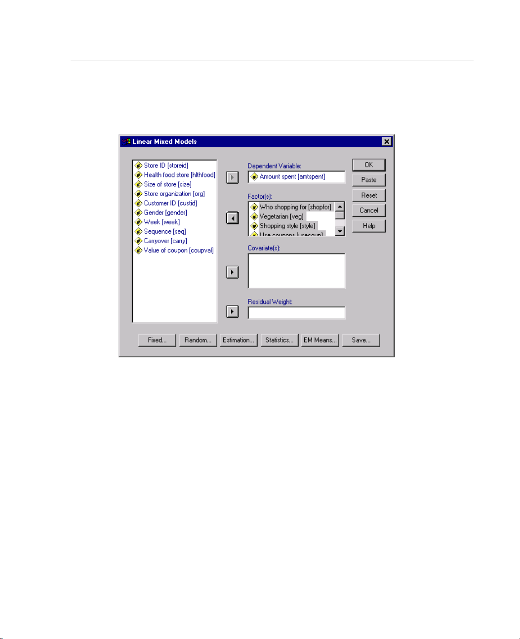
47
Obtaining a L
Figure 4-2
Linear Mixed Models dialog box
inear Mixed Models Analysis
Linear Mixed Mo
dels
E Select a dependent variable.
E Select at least one factor or covariate.
E Click Fixed or Random and specify at least a fixed-effects or random-effects model.
Optionally, select a weighting variable.
Page 58
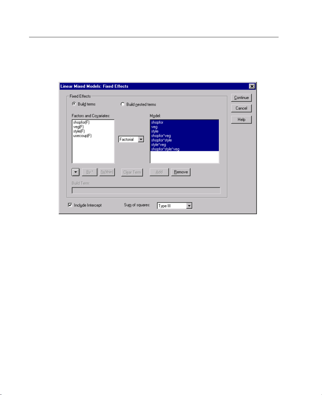
48
Chapter 4
Linear Mixed Models Fixed Effects
Figure 4-3
Linear Mixed
Fixed Effects. There is no default model, so you must explicitly specify the fixed
Models Fixed Effects dialog box
effects. Alternatively, you can build nested or non-nested terms.
Includ
e Intercept.
The intercept is usually included in the model. If you can assume
the data pass through the origin, you can exclude the intercept.
Sum of sq uares. The method of calculating the sums of squares. For models with no
g cells, the Type III method is most commonly used.
missin
Build Non-Nested Terms
For the selected factors and covariates:
Factorial. Creates all possible interactions and main effects of the selected variables.
s the default.
This i
Interaction. Creates the highest-level interaction term of all selected variables.
Page 59
49
Linear Mixed Mo
Main Effects. Creates a main-effects term for each variable selected.
All 2-Way. Creates all possible two-way interactions of the selected variables.
All 3-Way. Cr
All 4-Way. Creates all possible four-way interactions of the selected variables.
All 5-Way. Creates all possible five-way interactions of the selected variables.
Build Nested
You can build
eates all possible three-way interactions of the selected variables.
Terms
nested terms for your model in this procedure. Nested terms are
useful for modeling the effect of a factor or covariate whose values do not interact
with the levels of another factor. For example, a grocery store chain may follow the
spending of
their customers at several store locations. Since each customer frequents
only one of those locations, the Customer effect can be said to be nested within
the Store location effect.
Additiona
lly, you can include interaction effects or add multiple levels of nesting
to the nested term.
Limitations. Nested terms have the following restrictions:
All factors within an interaction must be unique. Thus, if A is a factor, then
specifying A*A is invalid.
Allfactorswithinanestedeffectmustbeunique.Thus,ifA is a factor, then
specifyin
No effect
g A(A) is invalid.
canbenestedwithinacovariate.Thus,ifA is a factor and X is a
covariate, then specifying A(X) is invalid.
dels
Sum of Squ
ares
For the mo
del, you can choose a type of sums of squares. Type III is the most
commonly used and is the default.
Page 60
50
Chapter 4
Type I. This method is also known as the hierarchical decomposition of the
sum-of-squares method. Each term is adjusted only for the term that precedes it in the
model. Type
A balanced
I sums of squares are commonly used for:
ANOVA model in which any main effects are specified before any
first-order interaction effects, any first-order interaction effects are specified
before any second-order interaction effects, and so on.
A polynomial regression model in which any lower-order terms are specified
before any h
Apurelyne
igher-order terms.
sted model in which the first-specified effect is nested within the
second-specified effect, the second-specified effect is nested within the third, and
so on. (This form of nesting can be specified only by using syntax.)
Type III. The default. This method calculates the sums of squares of an effect in the
design as the sums of squares adjusted for any other effects that do not contain it and
orthogona
l to any effects (if any) that contain it. The Type III sums of squares have
one major advantage in that they are invariant with respect to the cell frequencies
as long as the general form of estimability remains constant. Hence, this type of
sums of sq
uares is o ften considered useful for an unbalanced model with no missing
cells. In a factorial design with no missing cells, this method is equivalent to the
Yates' weighted-squares-of-means technique. The Type III sum-of-squares method
is commo
Any mod
Any bal
nlyusedfor:
els listed in Type I.
anced or unbalanced model with no empty cells.
Page 61
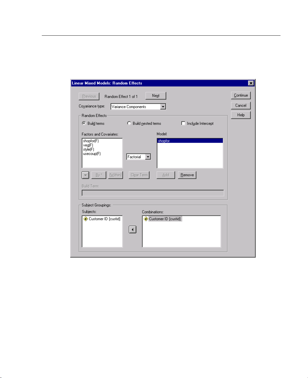
51
Linear Mixed Models Random Effects
Figure 4-4
Linear Mixed
Models Random Effects dialog box
Linear Mixed Mo
dels
Random Effects. There is no default model, so you must explicitly specify the random
effects. Alternatively, you can build nested or non-nested terms. You can also choose
to include an intercept term in the random-effects model.
You can specify multiple random-effects models. After building the first model,
Next to build the next model. Click Previous to scroll back through existing
click
models. Each random-effect model is assumed to be independent of every other
random-effect model; that is, separate covariance matrices will be computed for each.
Terms specified in the same random-effect model can be correlated.
Page 62
52
Chapter 4
Covariance type. This allows you to specify the covariance structure for the
random-effects model. A separate covariance matrix is estimated for each random
effect. The
Ante-Depe
AR(1)
AR(1): Hete
ARMA(1,1)
Compound Sy
Compound Sy
Compound Sy
Diagonal
Factor Anal
Factor Anal
Huynh-Feld
Scaled Iden
Toeplitz
Toeplitz: H
Unstructur
Unstructur
Variance Com
available structures are as follows:
ndence: First Order
rogeneous
mmetry
mmetry: Correlation Metric
mmetry: Heterogeneous
ytic: First Order
ytic: First Order, Heterogeneous
t
tity
eterogeneous
ed
ed: Correlation Metric
ponents
For more information, see “Covariance Structures” in Appendix B on page 125.
Subject Groupings. The variables listed are those that you selected as subject variables
in the Select Subjects/Repeated Variables dialog box. Choose some or all of these in
order to defi
ne the subjects for the random-effects model.
Page 63
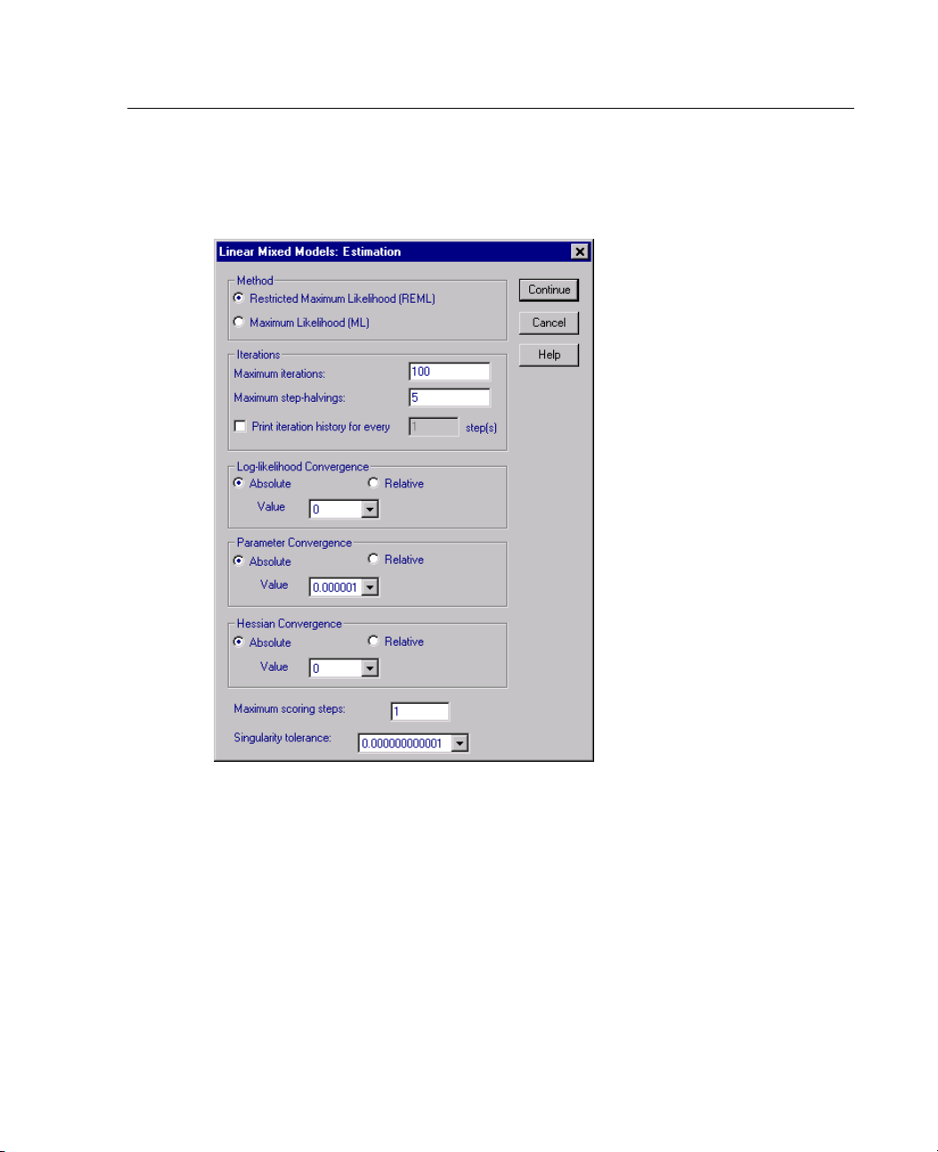
53
Linear Mixed Models Estimation
Figure 4-5
Linear Mixed
Models Estimation dialog box
Linear Mixed Mo
dels
Method. Select the maximum likelihood or restricted maximum likelihood estimation.
Iterations:
Maximum iterations. Specify a non-negative integer.
Page 64
54
Chapter 4
Maximum step-halvin gs. At each iteration, the step size is reduced by a factor
of 0.5 until
the log-likelihood increases or maximum step-halving is reached.
Specify a positive integer.
Print iteration history for every n step(s). Displays a table containing the
log-likelihood function value and parameter estimates at every n iterations
th
beginning w
ith the 0
iteration (the initial estimates). If you choose to print the
iteration history, the last iteration is always printed regardless of the value of n.
Log-likelihood Convergence. Convergenceis assumed if the absolute change or relative
change in t
he log-likelihood function is less than the value specified, which must be
non-negative. The criterion is not used if the value specified equals 0.
Parameter Convergence. Convergence is assumed if the maximum absolute change or
maximum re
lative change in the parameter estimates is less than the value specified,
which must be non-negative. The criterion is not used if the value specified equals 0.
Hessian Converg enc e. For the Absolute specification, convergence is assumed if
astatist
ic based on the Hessian is less than the value specified. For the
Relative
specification, convergence is assumed if the statistic is less than the product of the
value specified and the absolute value of the log-likelihood. The criterion is not used
if the va
lue specified equals 0.
Maximum sco ring steps. Requests to use the Fisher scoring algorithm up to iteration
number n. Specify a positive integer.
Singula
rity tolerance.
This is the value used as tolerance in checking singularity.
Specify a positive value.
Page 65
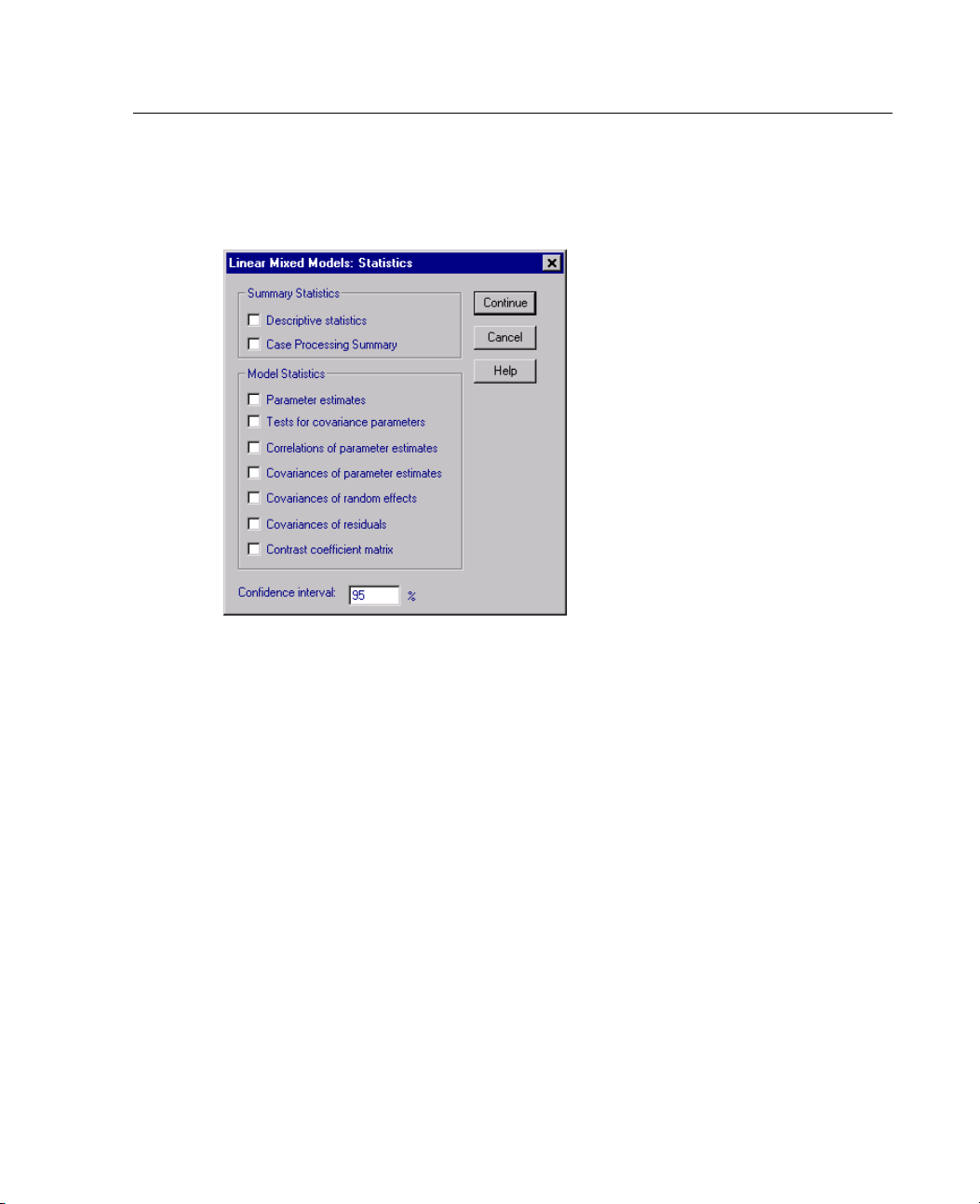
55
Linear Mixed Models Statistics
Figure 4-6
Linear Mixed
Summary Statistics. Produces tables for:
Descriptive statistics. Displays the sample sizes, means, and standard deviations
of the dependent variable and covariates (if specified). These statistics are
displa
Case P
measure variables, the repeated measure subjects, and the random-effects subjects
and their frequencies.
Models Statistics dialog box
yed for each distinct level combination of the factors.
rocessing Summary.
Linear Mixed Mo
dels
Displays the sorted values of the factors, the repeated
Model Sta tistics. Produces tables for:
Parameter estimates. Displays the fixed-effects and random-effects parameter
tes and their approximate standard errors.
estima
Tests
for covariance parameters.
Displays the asymptotic standard errors and Wald
tests for the covariance parameters.
Correlations of parameter estimates. Displays the asymptotic correlation matrix of
the fixed-effects parameter estimates.
Page 66
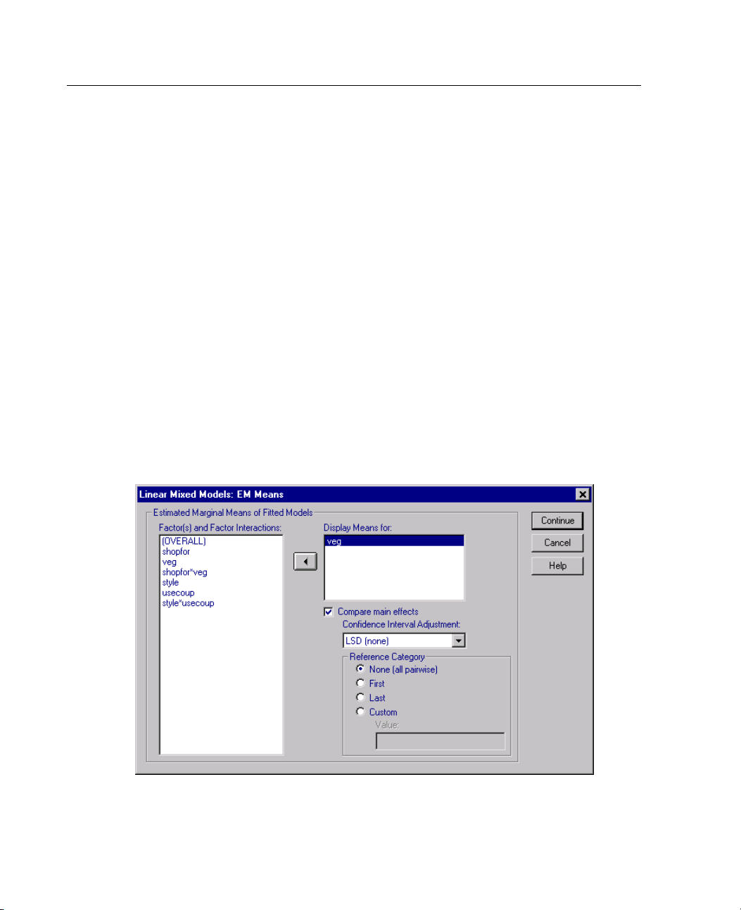
56
Chapter 4
Covariances of pa ram eter estimates. Displays the asymptotic covariance matrix of
the fixed-e
Covariance
ffects parameter estimates.
s of random effects.
Displays the estimated covariance matrix of
random effects. This option is available only when at least one random effect
is specified. If a subject variable is specified for a random effect, then the
common bloc
Covarianc
k is displayed.
es of residuals.
Displays the estimated residual covariance matrix. This
option i s available only when a repeated variable has been specified. If a subject
variable is specified, the common block is displayed.
Contrast coefficient matrix. This option displays the estimable functions used for
testing th
e fixed effects and the custom hypotheses.
Confidenc
Specify a value greater than or equal to 0 and less than 100. The default value is 95.
Linear Mix
Figure 4-7
Linear Mixed Models EM Means dialog box
e interval.
This value is used whenever a confidence interval is constructed.
ed Models EM Means
Page 67
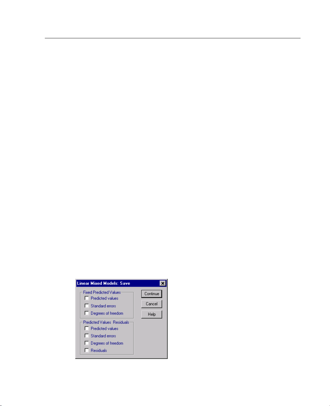
57
Linear Mixed Mo
Estimated Marginal Means of Fitted Models. This group allows you to request
dels
model-predicted estimated marginal means of the dependent variable in the cells
and their st
andard errors for the specified factors. Moreover, you can request that
factor levels of main effects be compared.
Factor(s) and Factor Interactions. This list contains factors and factor interactions
that have be
enspecifiedintheFixeddialogbox,plusan
OVERALL term. Model
terms built from covariates are excluded from this list.
Display Means for. The procedure will compute the estimated marginal means for
factors and factor interactions selected to this list. If
estimated
marginal means of the dependent variable are displayed, collapsing
OVERALL is selected, the
over all factors. Note that any selected factors or factor interactions remain
selected unless an associated variable has been removed from the Factors list in
the main d
Compare
ialog box.
main effects.
This option allows you to request pairwise comparisons
of levels of selected main effects. The Confidence Interval Adjustment allows
you to apply an adjustment to the confidence intervals and significance values
to accoun
t for multiple comparisons. The available methods are LSD (no
adjustment), Bonferroni, and Sidak. Finally, for each factor, you can select
a reference category to which comparisons are made. If no reference category
is selec
ted, all pairwise comparisons will be constructed. The options for the
reference category are first, last, or custom-specified (in which case, you enter
the value of the reference category).
Linear
Mixed Models Save
Figure 4-8
Linear Mixed Models Save dialog box
Page 68
58
Chapter 4
This dialog box allows you to save various model results to the working file.
Fixed Predicted Values. Saves variables related to the regression means without the
effects.
Predicted values. The regression means without the random effects.
Standard errors. The standard errors of the estimates.
Degrees of freedom. The degrees of freedom associated with the estimates.
Predicted Values and Residuals. Saves variables related to the model fitted value.
Predicted values. The model fitted value.
Standard errors. The standard errors of the estimates.
Degrees of freedom. The degrees of freedom associated with the estimates.
Residuals. The data value minus the predicted value.
MIXED Command Additional Features
The SPSS command language also allows you to:
Specify tests of effects versus a linear combination of effects or a value (using the
TEST subcom
Include us
Compute es
WITH keyword of the EMMEANS subcommand).
Compare simple main effects of interactions (using the EMMEANS subcommand).
mand).
er-missing values (using the
timated marginal means for specified values of covariates (using the
MISSING subcommand).
See the SPSS
Command Syntax Reference for complete syntax information.
Page 69
Chapter
5
Model Select
The Model Selection Loglinear Analysis procedure analyzes multiway
crosstabul
multidimensional crosstabulations using an iterative proportional-fitting algorithm.
This procedure helps you find out which categorical variables are associated. To
build mode
saturated models, you can request parameter estimates and tests of partial association.
A saturated model adds 0.5 to all cells.
Example.
counted people in each group, combining various categories of water softness (soft,
medium, or hard), previous use of one of the brands, and washing temperature
(cold or h
brand preference.
Statistics. Frequencies, residuals, parameter estimates, standard errors, confidence
interva
and normal probability plots.
ations (contingency tables). It fits hierarchical loglinear models to
ls, forced entry and backward elimination methods are available. For
In a study of user preference for one of two laundry detergents, researchers
ot). They found how temperature is related to water softness and also to
ls, and tests of partial association. For custom models, plots of residuals
ion Loglinear Analysis
Model Se
Data. Fa
Categorical string variables can be recoded to numeric variables before starting
the model selection analysis.
a situation where many cells have small numbers of observations, and the chi-square
values may not be useful.
lection Loglinear Analysis Data Considerations
ctor variables are categorical. All variables to be analyzed must be numeric.
Avoid s
pecifying many variables with many levels. Such specifications can lead to
59
Page 70
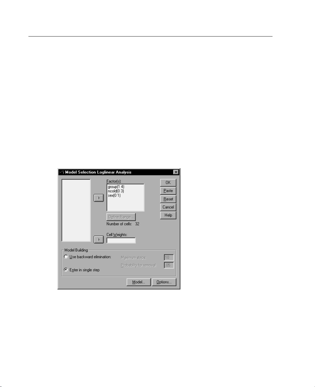
60
Chapter 5
Related procedures. The Model Selection procedure can help identify the terms
needed in the model. Then you can continue to evaluate the model using General
Loglinear A
nalysis or Logit Loglinear Analysis. You can use Autorecode to recode
string variables. If a numeric variable has empty categories, use Recode to create
consecutive integer values.
Obtaining a Model Selection Loglinear Analysis
From the menus choose:
Analyze
Loglinear
Model Selection...
Figure 5-1
Model Selection Loglinear Analysis dialog box
E Select two or more numeric categorical factors.
E Select one or more factor variables in the Factor(s) list, and click Define Range.
E Define the range of values for each factor variable.
E Select an option in the Model Building group.
Page 71
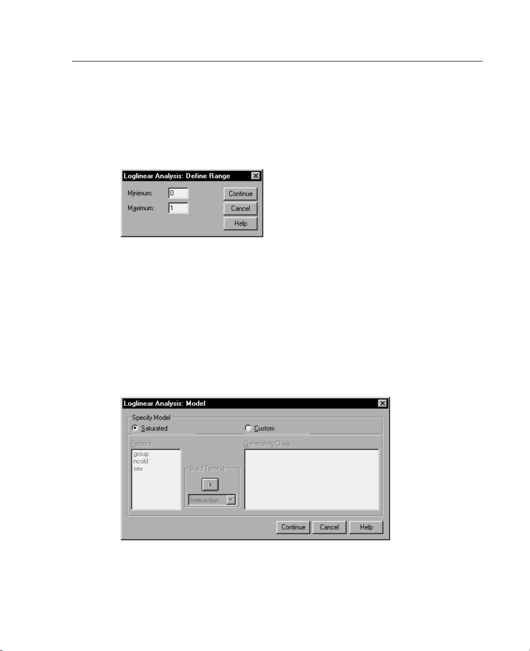
61
Optionally, you can select a cell weight variable to specify structural zeros.
Loglinear A
nalysis Define Range
Figure 5-2
Loglinear Analysis Define Range dialog box
You must indicate the range of categories for each factor variable. Values for
Minimum and Maximum correspond to the lowest and highest categories of the factor
variable
. Both values must be integers, and the minimum value must be less than the
maximum value. Cases with values outside of the bounds are excluded. For example,
if you specify a minimum value of 1 and a maximum value of 3, only the values 1, 2,
and3areu
sed. Repeat this process for each factor variable.
Loglinear Analysis Model
Model Selectio
n Loglinear Analysis
Figure 5-3
Loglinear Analysis Model dialog box
Page 72
62
Chapter 5
Specify Model. A saturated model contains all factor main effects and all
factor-by-factor interactions. Select Custom to specify a generating class for an
unsaturate
Generating Class. A generating class is a list of the highest-order terms in which
dmodel.
factors appear. SPSS builds a hierarchical model containing the terms that define the
generating
C in the Factors list and then select
class and all lower-order relatives. Suppose you select variables A, B,and
Interaction from the Build Terms drop-down list.
The resulting model will contain the specified 3-way interaction A*B*C, the 2-way
interacti
ons A*B, A*C,andB*C, and main effects for A, B,andC.Donotspecifythe
lower-order relatives in the generating class.
Build Ter
ms
For the se
Interaction. Creates the highest-level interaction term of all selected variables. This is
the default.
Main effe
All 2-way. Creates all possible two-way interactions of the selected variables.
All 3-way. Creates all possible three-way interactions of the selected variables.
All 4-way
All 5-way. Creates all possible five-way interactions of the selected variables.
lected factors and covariates:
cts.
Creates a main-effects term for each variable selected.
.
Creates all possible four-way interactions of the selected variables.
Page 73
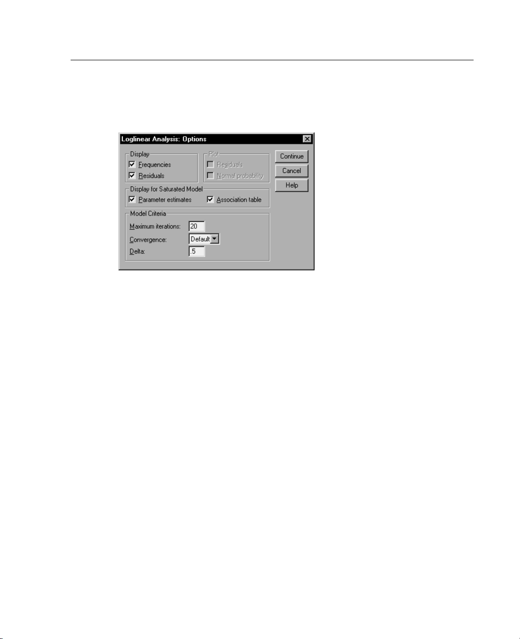
63
Model Selection Loglinear Analysis Options
Figure 5-4
Loglinear An
Display. You can choose Frequencies, Residuals, or both. In a saturated model, the
observed and expected frequencies are equal, and the residuals are equal to 0.
Display for Saturated Model. For a saturated model, you can choose Parameter
estimates
from the model. An association table, which lists tests of partial association, is also
available. This option is computationally expensive for tables with many factors.
alysis Options dialog box
. The parameter estimates may help determine which terms can be dropped
Model Selectio
n Loglinear Analysis
Plot. For custom models, you can choose one or both types of plots, Residuals and
Normal probability. These will help determine how well a model fits the data.
Model Criteria. SPSS uses an iterative proportional-fitting algorithm to obtain
parameter estimates. You can override one or more of the estimation criteria by
specifying
Maximum iterations, Convergence,orDelta (a value added to all cell
frequencies for saturated models).
HILOGLINEAR Command Additional Features
The SPSS command language also allows you to:
Specify cell weights in matrix form (using the CWEIGHT subcommand).
Generate analyses of several models with a single command (using the DESIGN
subcommand).
Page 74
64
Chapter 5
See the SPSS Command Syntax Reference for complete syntax information.
Page 75
Chapter
6
General Logl
The General Loglinear Analysis procedure analyzes the frequency counts of
observatio
a contingency table. Each cross-classification in the table constitutes a cell, and
each categorical variable is called a factor. The dependent variable is the number of
cases (fre
factors and covariates. This procedure estimates maximum likelihood parameters of
hierarchical and nonhierarchical loglinear models using the Newton-Raphson method.
Either a P
You can select up to 10 factors to define the cells of a table. A cell structure variable
allows you to define structural zeros for incomplete tables, include an offset term in
the model
tables. Contrast variables allow computation of generalized log-odds ratios (GLOR).
SPSS automatically displays model information and goodness-of-fit statistics.
You can a
values in the working data file.
Example. Data from a report of automobile accidents in Florida are used to determine
the rela
nonfatal. The odds ratio indicates significant evidence of a relationship.
ns falling into each cross-classification category in a crosstabulation or
quency) in a cell of the crosstabulation, and the explanatory variables are
oisson or a multinomial distribution can be analyzed.
, fit a log-rate model, or implement the method of adjustment of marginal
lso display a variety of statistics and plots or save residuals and predicted
tionship between wearing a seat belt and whether an injury was fatal or
inear Analysis
Statistics. Observed and expected frequencies; raw, adjusted, and deviance residuals;
design m
and confidence intervals. Plots: adjusted residuals, deviance residuals, and normal
probability.
atrix; parameter estimates; odds ratio; log-odds ratio; GLOR; Wald statistic;
65
Page 76
66
Chapter 6
General Logl
Data. Facto
is in the model, SPSS applies the m ean covariate value for cases in a cell to that
cell. Contrast variables are continuous. They are used to compute generalized
log-odds ra
combination of the logs of the expected cell counts.
A cell structure variable assigns weights. For example, if some of the cells are
structura
a cell structure variable to weight aggregated data. Instead, choose
fromtheDatamenu.
Assumptio
and multinomial.
Under the Poisson distribution assumption:
The total sample size is not fixed before the study, or the analysis is not
conditional on the total sample size.
The event of an observation being in a cell is statistically independent of the cell
counts of
Under the multinomial distribution assumption:
The total sample size is fixed, or the analysis is conditional on the total sample
size.
The cell
inear Analysis Data Considerations
rs are categorical, and cell covariates are continuous. When a covariate
tios. The values of the contrast variable are the coefficients for the linear
l zeros, the cell structure variable has a value of either 0 or 1. Do not use
Weight Cases
ns.
Two distributions are available in General Loglinear Analysis: Poisson
other cells.
counts are not statistically independent.
Related procedures. Use t he Crosstabs procedure to examine the crosstabulations. Use
the Logit Loglinear procedure when it is natural to regard one or more categorical
variable
sastheresponsevariablesandtheothersastheexplanatoryvariables.
Obtaining a General Loglinear Analysis
E From the menus choose:
Analyze
Logline
General.
ar
..
Page 77
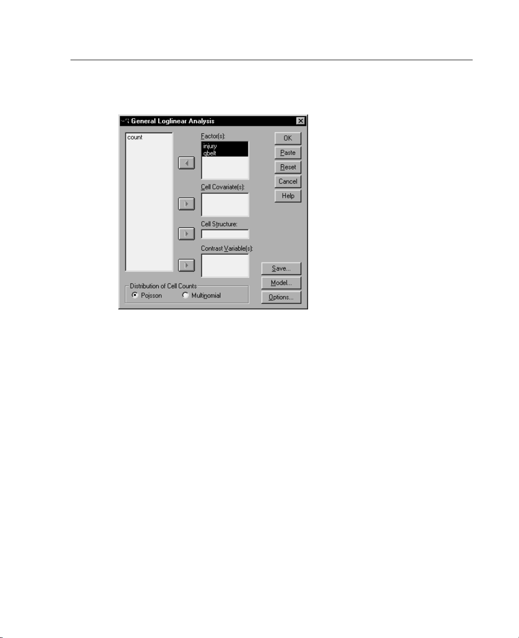
67
General Loglin
Figure 6-1
General Loglinear Analysis dialog box
E In the General Loglinear Analysis dialog box, select up to 10 factor variables.
ear Analysis
Optionally, you can:
Select cell covariates.
Select a cell structure variable to define structural zeros or include an offset term.
Select a contrast variable.
Page 78
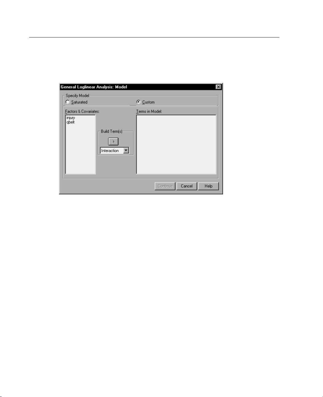
68
Chapter 6
General Loglinear Analysis Model
Figure 6-2
General Logl
Specify Model. A saturated model contains all main effects and interactions involving
inear Analysis Model dialog box
factor variables. It does not contain covariate terms. Select Custom to specify only a
subset of interactions or to specify factor-by-covariate interactions.
Factors and Covariates. The factors and covariates are listed, with (Cov) indicating
acovariate.
Terms in Mod el. The model depends on the nature of your data. After selecting
Custom, you can select the main effects and interactions that are of interest in your
analysis. You must indicate all of the terms to be included in the model.
Build Terms
For the selected factors and covariates:
Interaction. Creates the highest-level interaction term of all selected variables. This is
the default.
Main effects. Creates a main-effects term for each variable selected.
All 2-way. Creates all possible two-way interactions of the selected variables.
Page 79
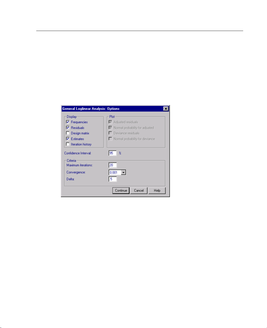
69
All 3-way. Creates all possible three-way interactions of the selected variables.
All 4-way. Creates all possible four-way interactions of the selected variables.
All 5-way. Cr
eates all possible five-way interactions of the selected variables.
General Loglinear Analysis Options
Figure 6-3
General Loglinear Analysis Options dialog box
General Loglin
ear Analysis
The General Loglinear Analysis procedure displays model information and
goodness-of-fit statistics. In addition, you can choose one or more of the following:
Display. Several statistics are available for display—observed and expected cell
frequencies; raw, adjusted, and deviance residuals; a design matrix of the model;
and parameter estimates for the model.
Plot. Plots, available for custom models only, include two scatterplot matrices
(adjusted residuals or deviance residuals against observed and expected cell counts).
You can also display normal probability and detrended normal plots of adjusted
residuals or deviance residuals.
Confidence Interval. The confidence interval for parameter estimates can be adjusted.
Page 80
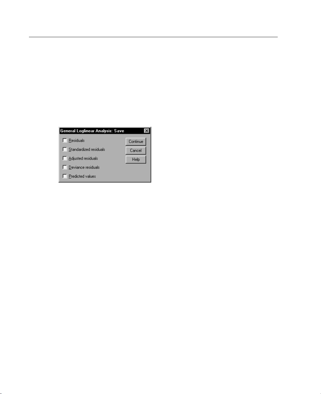
70
Chapter 6
Criteria. TheNewton-Raphsonmethodisusedtoobtainmaximumlikelihood
parameter estimates. You can enter new values for the maximum number of
iterations
, t he convergence criterion, and delta (a constant added to all cells for initial
approximations). Delta remains in the cells for saturated models.
General Log
Figure 6-4
General Loglinear Analysis Save dialog box
Select the values you want to save as new variables in the working data file. The
suffix n in the new variable names increments to make a unique name for each saved
variable.
if the data are recorded in individual observations in the Data Editor. If you save
residuals or predicted values for unaggregated data, the saved value for a cell in the
contingency table is entered in the Data Editor for each case in that cell. To make
sense of the saved values, you should aggregate the data to obtain the cell counts.
The predicted values can also be saved.
Residuals. Also called the simple or raw residual, it is the difference between the
Standardized Residuals. The residual divided by an estimate of its standard error.
linear Analysis Save
The saved values refer to the aggregated data (cells in the contingency table), even
Four types of residuals can be saved: raw, standardized, adjusted, and deviance.
observed cell count and its expected count.
Standardized residuals are also known as Pearson residuals.
Page 81
71
Deviance Residuals. The signed square root of an individual contribution to the
GENLOG Com
The SPSS command language also allows you to:
Calculate linear combinations of observed cell frequencies and expected cell
Change the default threshold value for redundancy checking (using the CRITERIA
Display the standardized residuals (using the PRINT subcommand).
See the SPSS Command Syntax Reference for complete syntax information.
General Loglin
Adjusted Residuals. The standardized residual divided by its e stimated standard
error. Sinc
e the adjusted residuals are asymptotically standard normal when the
ear Analysis
selected model is correct, they are preferred over the standardized residuals
for checking for normality.
likelihood
-ratio chi-square statistic (G squared), where the sign is the sign of the
residual (observed count minus expected count). Deviance residuals have an
asymptotic standard normal distribution.
mand Additional Features
frequenci
that combination (using the
subcommand).
es, and print residuals, standardized residuals, and adjusted residuals of
GERESID subcommand).
Page 82
Page 83
Chapter
7
Logit Loglin
The Logit Loglinear Analysis procedure analyzes the relationship between dependent
(or respons
variables are always categorical, while t he independent variables can be categorical
(factors). Other independent variables, cell covariates, can be continuous, but they
are not app
applied to that cell. The logarithm of the odds of the dependent variables is expressed
as a linear combination of parameters. A multinomial distribution is automatically
assumed;
procedure estimates parameters of logit loglinear models using the Newton-Raphson
algorithm.
You can se
structure variable allows you to define structural zeros for incomplete tables, include
an offset term in the model, fit a log-rate model, or implement the method of
adjustm
log-odds ratios (GLOR). The values of the contrast variable are the coefficients for
the linear combination of the logs of the expected cell counts.
SPSS aut
You can also display a variety of statistics and plots or save residuals and predicted
values in the working data file.
e) variables and independent (or explanatory) variables. The dependent
lied on a case-by-case basis. The weighted covariate mean for a cell is
these models are sometimes called multinomial logit models. This
lect from 1 to 10 dependent and factor variables combined. A cell
ent of marginal tables. Contrast variables allow computation of generalized
omatically displays model information and goodness-of-fit statistics.
ear Analysis
e.
Exampl
type vary with their size and the four lakes in which they live? The study found that
the odds of a smaller alligator preferring reptiles to fish is 0.70 times lower than for
larger
highest in lake 3.
A study in Florida included 219 alligators. How does the alligators' food
alligators; also, the odds of selecting primarily reptiles instead of fish were
73
Page 84
74
Chapter 7
Statistics. Observed and expected frequencies; raw, adjusted, and deviance residuals;
design matrix; parameter estimates; generalized log-odds ratio; Wald statistic; and
confidence
probability plots.
intervals. Plots: adjusted residuals, deviance residuals, and normal
Logit Logli
Data. The d
can be continuous, but when a covariate is in the model, SPSS applies the mean
covariate value for cases in a cell to that cell. Contrast variables are continuous. They
are used to
variable are the coefficients for the linear combination of the logs of the expected
cell counts.
structural zeros, the cell structure variable has a value of either 0 or 1. Do not use a
cell structure variable to weight aggregate data. Instead, use Weight Cases on the
Data menu
Assumptions. The counts within each combination of categories of explanatory
variables are assumed to have a multinomial distribution. Under the multinomial
distrib
The tot
The cell counts are not statistically independent.
Related
Use the General Loglinear Analysis procedure when you want to analyze the
relationship between an observed count and a set of explanatory variables.
near Analysis Data Considerations
ependent variables are categorical. Factors are categorical. Cell covariates
compute generalized log-odds ratios (GLOR). The values of the contrast
A cell str
size.
ucture variable assigns weights. For example, if some of the cells are
.
ution assumption:
al sample size is fixed, or the analysis is conditional on the total sample
procedures.
Use the Crosstabs procedure to display the contingency tables.
Obtaining a Logit Loglinear A nalysis
E From the menus choose:
Analyze
Loglinear
Logit...
Page 85
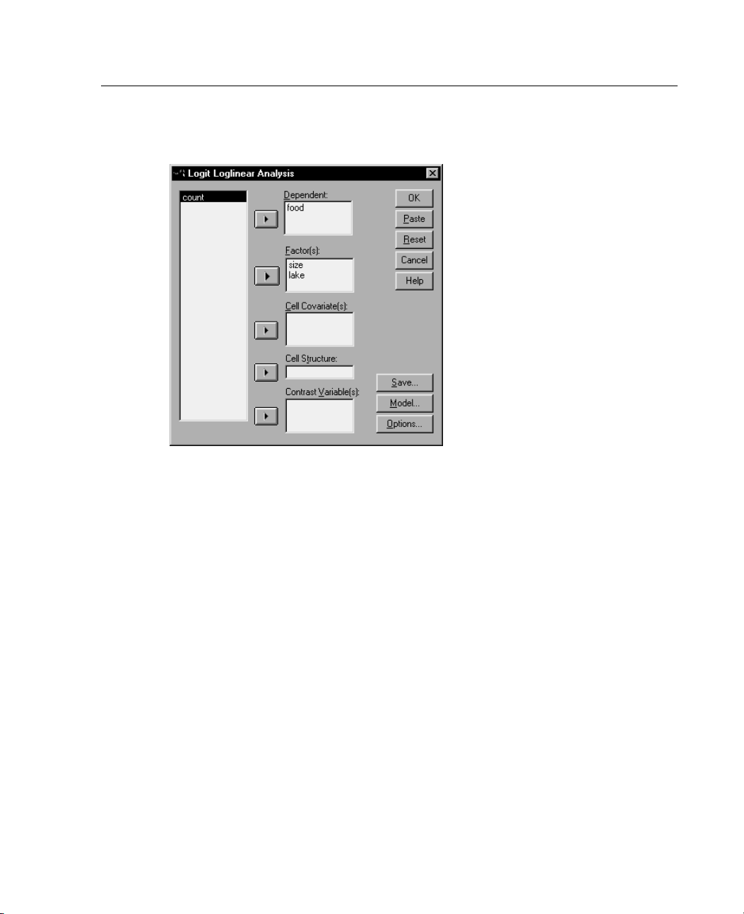
75
Figure 7-1
Logit Loglinear Analysis dialog box
E In the L
E Select
ogit Loglinear Analysis dialog box, select one or more dependent variables.
one or more factor variables.
Logit Loglinea
rAnalysis
The total number of dependent and factor variables must be less than or equal to 10.
Optionally, you can:
Select cell covariates.
Select a cell structure variable to define structural zeros or include an offset term.
Select one o r more contrast variables.
Page 86
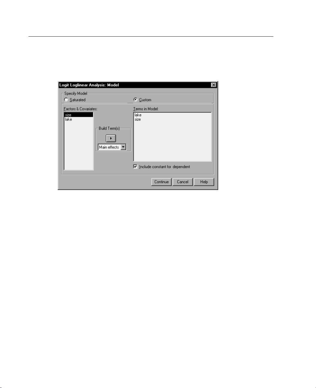
76
Chapter 7
Logit Loglinear Analysis Model
Figure 7-2
Logit Loglin
Specify Model. A saturated model contains all main effects and interactions involving
ear Analysis Model dialog box
factor variables. It does not contain covariate terms. Select Custom to specify only a
subset of interactions or to specify factor-by-covariate interactions.
Factors and Covariates. The factors and covariates are listed, with (Cov) indicating
acovariate.
Terms in Mod el. The model depends on the nature of your data. After selecting
Custom, you can select the main effects and interactions that are of interest in your
analysis. You must indicate all of the terms to be included in the model.
Terms are added to the design by taking all possible combinations of the dependent
terms and matching each combination with each term in the model list. If
constant for dependent
is selected, there is also a unit term (1) added to the model list.
Include
For example, suppose variables D1 and D2 are the dependent variables. A
dependent terms list is created by the Logit Loglinear Analysis procedure (D1, D2,
D1*D2). If the Terms in Model list contains M1 and M2 and a constant is included,
the model list contains 1, M1,andM2. The resultant design includes combinations of
each model term with each dependent term:
D1, D2, D1*D2
Page 87
77
Logit Loglinea
M1*D1, M1*D2, M1*D1*D2
M2*D1, M2*D2, M2*D1*D2
Include constant for dependent. Includes a constant for the dependent variable in
acustommod
el.
Build Terms
For the selected factors and covariates:
Interaction. Creates the highest-level interaction term of all selected variables. This is
the default
Main effects. Creates a main-effects term for each variable selected.
All 2-way. Creates all possible two-way interactions of the selected variables.
All 3-way. C
All 4-way. Creates all possible four-way interactions of the selected variables.
All 5-way. Creates all possible five-way interactions of the selected variables.
.
reates all possible three-way interactions of the selected variables.
rAnalysis
Page 88
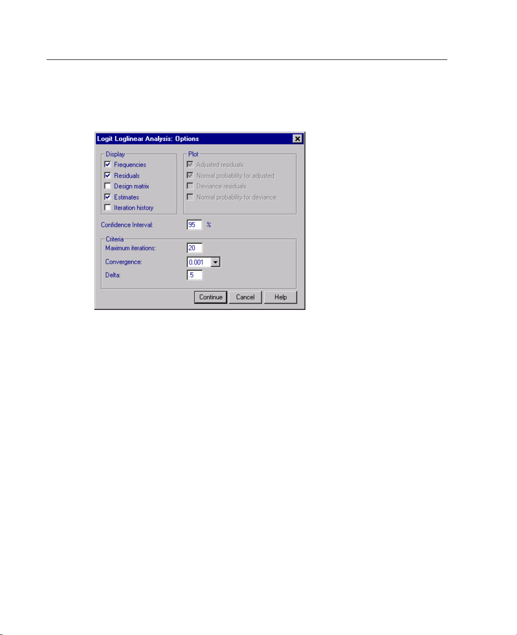
78
Chapter 7
Logit Loglinear Analysis Options
Figure 7-3
Logit Loglin
ear Analysis Options dialog box
The Logit Loglinear Analysis procedure displays model information and
goodness-of-fit statistics. In addition, you can choose one or more of the following
options:
Display. Several statistics are available for display: observed and expected cell
frequencies; raw, adjusted, and deviance residuals; a design matrix of the model;
and parameter estimates for the model.
Plot. Plots available for custom models include two scatterplot matrices (adjusted
residuals or deviance residuals against observed and expected cell counts). You can
also display normal probability and detrended normal plots of adjusted residuals
or deviance residuals.
Confidence Interval. The confidence interval for parameter estimates can be adjusted.
Criteria. TheNewton-Raphsonmethodisusedtoobtainmaximumlikelihood
parameter estimates. You can enter new values for the maximum number of
iterations, the convergence criterion, and delta (a constant added to all cells for initial
approximations). Delta remains in the cells for saturated models.
Page 89
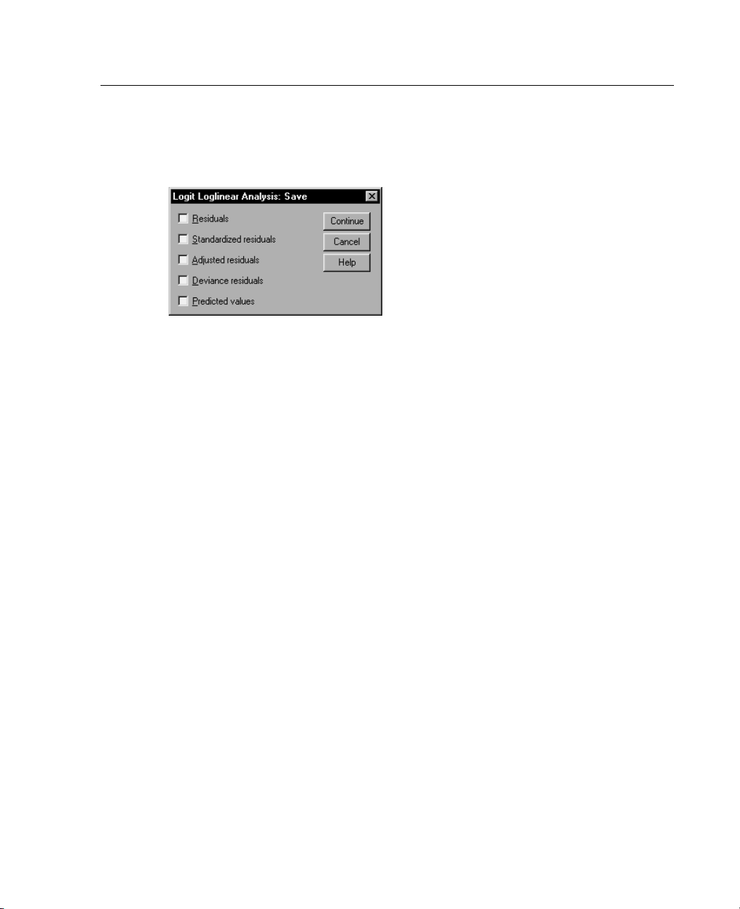
79
Logit Loglinear Analysis Save
Figure 7-4
Logit Loglin
Select the values you want to save as new variables in the working data file. The
suffix n in the new variable names increments to make a unique name for each saved
variable.
The saved values refer to the aggregated data (to cells in the contingency table),
even if the data are recorded in individual observations in the Data Editor. If you save
residuals or predicted values for unaggregated data, the saved value for a cell in the
contingency table is entered in the Data Editor for each case in that cell. To make
sense of the saved values, you should aggregate the data to obtain the cell counts.
Four types of residuals can be saved: raw, standardized, adjusted, and deviance.
The predicted values can also be saved.
Residuals. Also called the simple or raw residual, it is the difference between the
Standardized Residuals. The residual divided by an estimate of its standard error.
Adjusted Residuals. The standardized residual divided by its estimated standard
Deviance Residuals. The signed square root of an individual contribution to the
ear Analysis Save dialog box
observed cell count and its expected count.
Standardized residuals are also known as Pearson residuals.
error. Since the adjusted residuals are asymptotically standard normal when the
selected model is correct, they are preferred over the standardized residuals
for checking for normality.
likelihood-ratio chi-square statistic (G squared), where the sign is the sign of the
residual (observed count minus expected count). Deviance residuals have an
asymptotic standard normal distribution.
Logit Loglinea
rAnalysis
Page 90
80
Chapter 7
GENLOG Command Additional Features
The SPSS command language also allows you to:
Calculate linear combinations of observed cell frequencies and expected cell
frequencies
that combination (using the
Change the default threshold value for redundancy checking (using the CRITERIA
subcommand).
Display the standardized residuals (using the PRINT subcommand).
See the SPSS Command Syntax Reference for complete syntax information.
, and print residuals, standardized residuals, and adjusted residuals of
GERESID subcommand).
Page 91
Chapter
8
Ordinal Regr
Ordinal Regression allows you to model the dependence of a polytomous ordinal
response on
Ordinal Regression is based on the methodology of McCullagh (1980, 1998), and the
procedure is referred to as
Standard l
differences between a response (dependent) variable and a weighted combination of
predictor (independent) variables. The estimated coefficients reflect how changes in
the predic
sense that changes in the level of the response are equivalent throughout the range of
the response. For example, the difference in height between a person who is 150 cm
tall and a
difference in height between a person who is 210 cm tall and a person who is 200 cm
tall. These relationships do not necessarily hold for ordinal variables, in which the
choice a
Example. Ordinal Regression could be used to study patient reaction to drug dosage.
The possible reactions may be classified as “none,” “mild,” “moderate,” or “severe.”
The diff
quantify and is based on perception. Moreover, the difference between a mild and
moderateresponsemaybegreaterorlessthanthedifferencebetweenamoderateand
severe
a set of predictors, which can be factors or covariates. The design of
inear regression analysis involves minimizing the sum-of-squared
tors affect the response. The response is assumed to be numerical, in the
person who is 140 cm tall is 10 cm, which has the same meaning as the
nd number of response categories can be quite arbitrary.
erence between a mild and moderate reaction is difficult or impossible to
response.
ession
PLUM in the syntax.
Statistics and plots. Observed and expected frequencies and cumulative frequencies,
Pearson residuals for frequencies and cumulative frequencies, observed and expected
bilities, observed and expected cumulative probabilities of each response
proba
category by covariate pattern, asymptotic correlation and covariance matrices
of parameter estimates, Pearson's chi-square and likelihood-ratio chi-square,
ess-of-fit statistics, iteration history, test of parallel lines assumption, parameter
goodn
81
Page 92
82
Chapter 8
estimates, standard errors, confidence intervals, and Cox and S nell's, Nagelkerke's,
and McFadden's R2statistics.
Ordinal Regression Data Considerations
Data. The dependent variable is assumed to be ordinal and can be numeric or
string. The ordering is determined by sorting the values of the dependent variable
in ascendi
assumed to be categorical. Covariate variables must be numeric. Note that using
more than one continuous covariate can easily result in the creation of a very large
cell proba
Assumptions. Only one response variable is allowed, and it must be specified. Also,
for each distinct pattern of values across the independent variables, the responses
are assum
Related procedures. Nominal logistic regression uses similar models for nominal
dependent variables.
ng order. The lowest value defines the first category. Factor variables are
bilities table.
ed to be independent multinomial variables.
Obtaining an Ordinal Regression
E From the menus choose:
Analyze
Regression
Ordinal...
Page 93
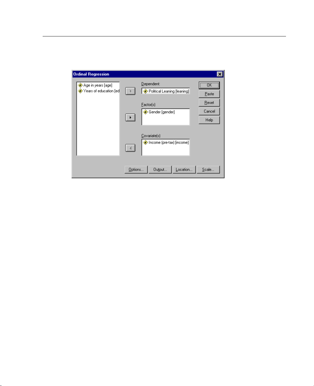
83
Figure 8-1
Ordinal Regression dialog box
E Select one dependent variable.
E Click OK.
Ordinal Regres
sion
Ordinal Regression Options
The Options dialog box allows you to adjust parameters used in the iterative
estimation algorithm, choose a level of confidence for your parameter estimates, and
select a link function.
Page 94
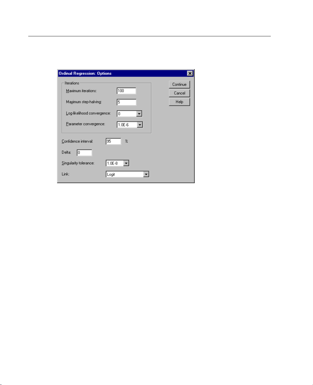
84
Chapter 8
Figure 8-2
Ordinal Regression Options dialog box
Iterations. You can customize the iterative algorithm.
Maximum iterations. Specify a non-negative integer. If 0 is specified, the
procedure returns the i nitial estimates.
Maximum step-halving. Specify a positive integer.
Log-likelihood convergence. The algorithm stops if the absolute or relative change
in the log-likelihood is less than this value. The criterion is not used if 0 is
specified.
Parameter convergence. The algorithm stops if the absolute or relative change
in each of the parameter estimates is less than this value. The criterion is not
used if 0 is specified.
Confidence interval. Specify a value greater than or equal to 0 and less than 100.
Delta. The value added to zero cell frequencies. Specify a non-negative value less
than 1.
Singularity tolerance. Used for checking for highly dependent predictors. Select a
value from the list of options.
Page 95
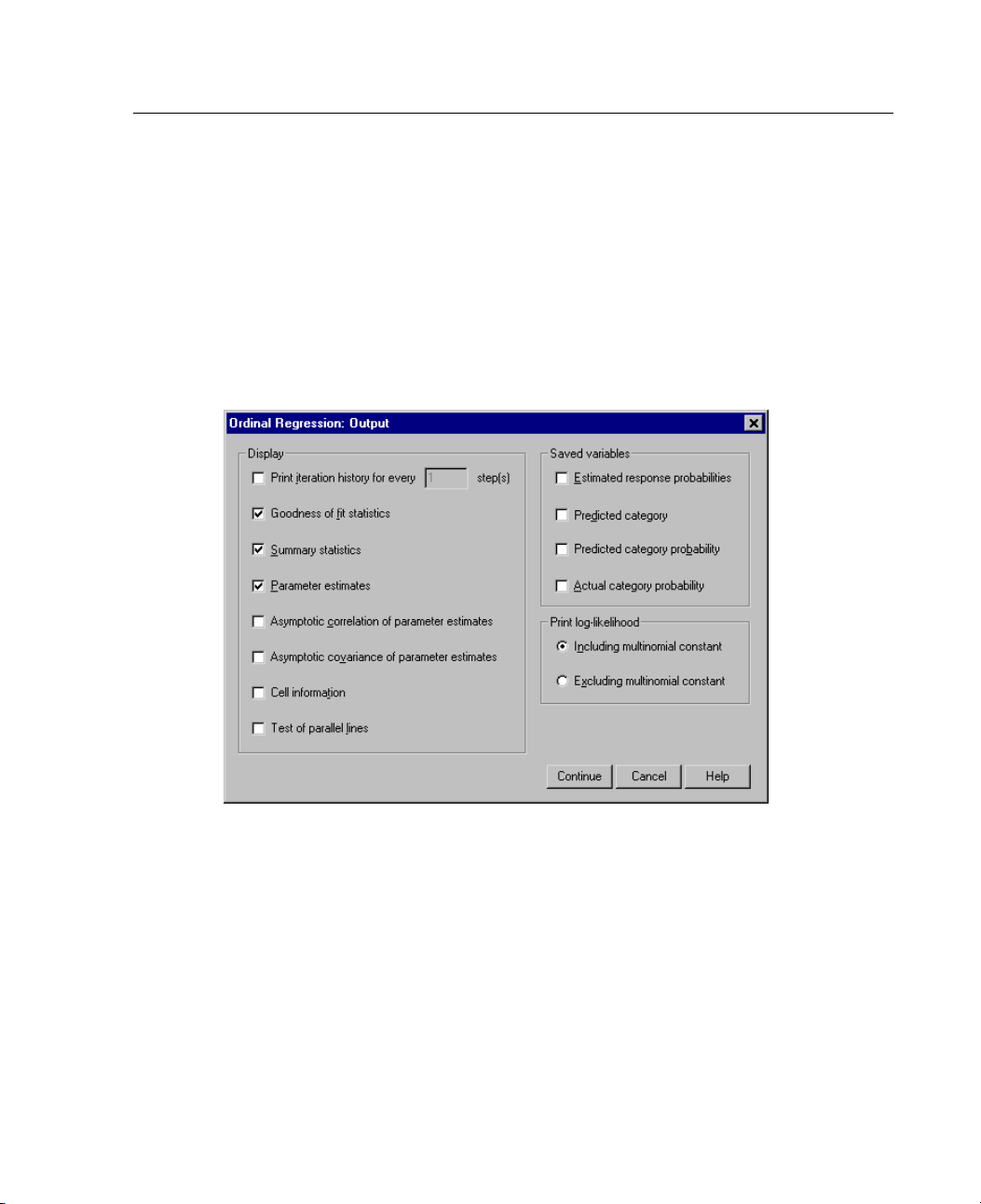
85
Link. Choose among the Cauchit, Complementary Log-log, Logit, Negative Log-log,
and Probit functions.
Ordinal Regression Output
The Output dialog box allows you to produce tables for display in the Viewer and
save variables to the working file.
Figure 8-3
Ordinal Regression Output dialog box
Ordinal Regres
sion
Display. Produces tables for:
Print ite ration history. The log-likelihood and parameter estimates are printed for
nt iteration frequency specified. The first and last iterations are always
the pri
printed.
Goodness-of-fit statistics. The Pearson and likelihood-ratio chi-square statistics.
They are computed based on the classification specified in the variable list.
Summary statistics. Cox and Snell's, Nagelkerke's, and McFadden's R
Parameter estimates. Parameter estimates, standard errors, and confidence
vals.
inter
2
statistics.
Page 96
86
Chapter 8
Asymptotic correla tion of parameter estimates. Matrix of parameter estimate
correlatio
Asymptotic
ns.
covariance of parameter estimates.
Matrix of parameter estimate
covariances.
Cell information. Observed and expected frequencies and cumulative frequencies,
Pearson residuals for frequencies and cumulative frequencies, observed and
expected pr
obabilities, and observed and expected cumulative probabilities of
each response category by covariate pattern. Note that for models with many
covariate patterns (for example, models with continuous covariates), this option
can genera
Test of pa
te a very large, unwieldy table.
rallel lines.
Test of the hypothesis that the location parameters are
equivalent across the levels of the dependent variable. This is available only
for the location-only model.
Saved variables. Saves the following variables to the working file:
Estimated response probabilities. Model-estimated probabilities of classifying
a factor/
covariate pattern into the response categories. There are as many
probabilities as the number of response categories.
Predicted category. The response category that has the maximum estimated
probability for a factor/covariate pattern.
Predicted category probability. Estimated probability of classifying a
factor/c
ovariate pattern into the predicted category. This probability is also the
maximum of the estimated probabilities of the factor/covariate pattern.
Actual categ ory probability. Estimated probability of classifying a factor/covariate
pattern into the actual category.
Print log-like lihood. Controls the display of the log-likelihood. Including multinomial
constant
product
gives you the full value of the likelihood. To compare your results across
s that do not include the constant, you can choose to exclude it.
Ordinal Regression Location Model
The Location dialog box allows you to specify the location model for your analysis.
Page 97
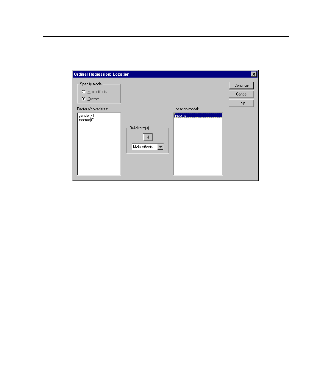
87
sion
Figure 8-4
Ordinal Regression Location dialog b ox
Specify
model.
A main-effects model contains the covariate and factor main effects
Ordinal Regres
but no interaction effects. You can create a custom model to specify subsets of factor
interactions or covariate interactions.
Factor
s/covariates.
The factors and covariates are listed with (F) forfactorand(C)
for covariate.
Location model. The model depends on the main effects and interaction effects that
you sel
ect.
Build Terms
For the selected factors and covariates:
Interaction. Creates the highest-level interaction term of all selected variables.
fects.
Main ef
All 2-way. Creates all possible two-way interactions of the selected variables.
All 3-way. Creates all possible three-way interactions of the selected variables.
All 4-w
Creates a main-effects term for each variable selected.
ay.
Creates all possible four-way interactions of the selected variables.
Page 98
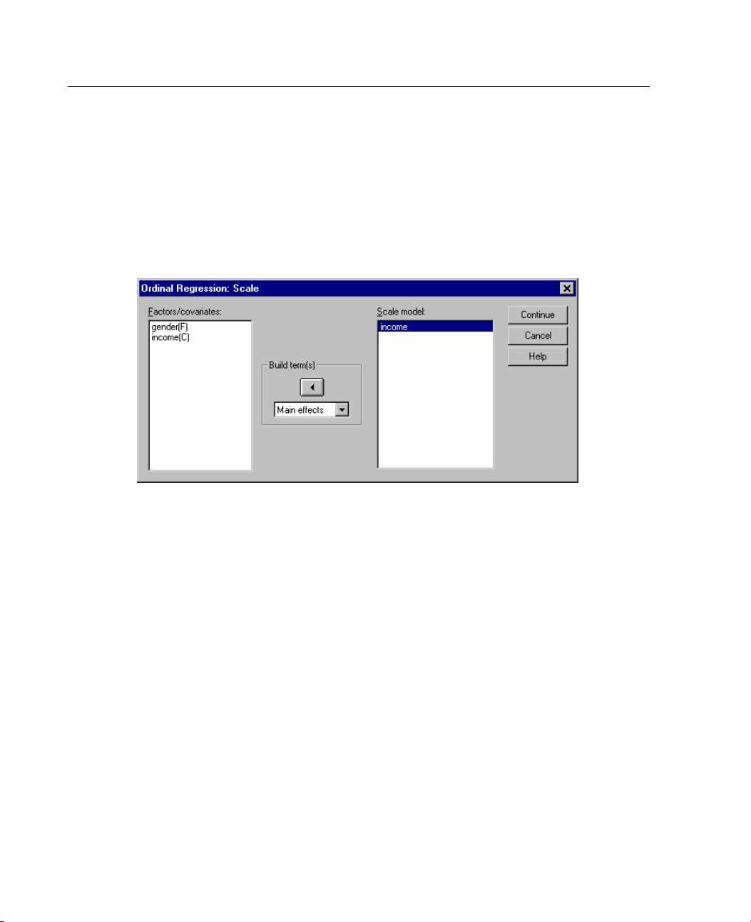
88
Chapter 8
All 5-way. Creates all possible five-way interactions of the selected variables.
Ordinal Reg
The S cale di
Figure 8-5
Ordinal Regression Scale dialog box
Factors/covariates. The factors and covariates are listed with (F) forfactorand(C)
for covariate.
Scale model. The model depends on the main and interaction effects that you select.
Build Terms
ression Scale Model
alog box a llows you to specify the scale model for your analysis.
For the selected factors and covariates:
Interaction. Creates the highest-level interaction term of all selected variables.
Main effects. Creates a main-effects term for each variable selected.
All 2-way. Creates all possible two-way interactions of the selected variables.
All 3-way. Creates all possible three-way interactions of the selected variables.
All 4-way. Creates all possible four-way interactions of the selected variables.
All 5-way. Creates all possible five-way interactions of the selected variables.
Page 99
89
PLUM Command Additional Features
You can customize your Ordinal Regression if you paste your selections into a
syntax window and edit the resulting PLUM command syntax. The SPSS command
language al
Create cus
See the SPSS
so allows you to:
tomized hypothesis tests by specifying null hypotheses as linear
combinations of parameters.
Command Syntax Reference for complete syntax information.
Ordinal Regres
sion
Page 100
 Loading...