

Page 1
SPSS® 13.0 Brief Guide
Page 2

For more information about SPSS®softwareproducts,pleasevisitourWeb site at http://www.spss.com or contact
SPSS Inc.
233 South Wacker Drive, 11th Floor
Chicago, IL 60606-6412
Tel: (312) 651
-3000
Fax: (312) 651-3668
SPSS is a registered trademark and the other product names are the trademarks of SPSS Inc. for its proprietary
computer soft
ware. No material describing such software may be produced or distributed without the written
permission of the owners of the trademark and license rights in the software and the copyrights in the published
materials.
The SOFTWARE a
nd documentation are provided with RESTRICTED RIGHT S. Use, duplication, or disclosure
by the Government is subject to restrictions as set forth in subdivision (c) (1) (ii) of The Rights in Technical Data
and Computer Software clause at 52.227-7013. Contractor/manufacturer is SPSS Inc., 233 South Wacker Drive,
11thFloor,C
hicago, IL 60606-6412.
General notice: Other product names mentioned herein are used for identification purposes only and may b e
trademarks of their respective companies.
TableLook is
a trademark of SPSS Inc.
Windows is a registered trademark of Microsoft Corporation.
DataDirect, DataDirect Connect, INTERSOLV, and SequeLink are registered trademarks of DataDirect
Technologie
s.
Portions of this product were created using LEADTOOLS © 1991–2000, LEAD Technologies, Inc. ALL
RIGHTS RESERVED.
LEAD, LEADTO
OLS, and LEADVIEW are registered trademarks of LEAD Technologies, Inc.
Sax Basic is a trademark of Sax Software Corporation. Copyright © 1993–2004 by Polar Engineering and
Consulting. All rights reserved.
Portions of t
his product were based on the work of the FreeType Team (http://www.freetype.org).
A portion of the SPSS software contains zlib technology. Copyright © 1995–2002 by Jean-loup Gailly and Mark
Adler. The zlib software is provided “as is,” without express or implied warranty.
A portion of t
he SPSS software contains Sun Java Runtime libraries. Copyright © 2003 by Sun Microsystems,
Inc. All rights reserved. The Sun Java Runtime libraries include code licensed from RSA Security, Inc. Some
portions of the libraries are licensed from IBM and are available at http://oss.software.ibm.com/icu4j/.
SPSS® 13.0 B r
ief Guide
Copyright © 2004 by SPSS Inc.
All rights r eserved.
Printed in the
United States of America.
No part of this publication m ay be reproduced, stored in a retrieval system, or transmitted, in any form or by any
means, electronic, mechanical, photocopying, recording, or otherwise, without the prior written permission
of the publis
her.
ISBN 0-13-154242-7
Page 3

SPSS 13.0
Preface
The SPSS® 13.0 Brief Guide provides a set of tutorials designed to acquaint you
with the va
tutorials in sequence or turn to the topics for which you need additional information.
You can use this guide as a supplement to the online tutorial that is included with
the SPSS B
found here.
rious components of the SPSS system. You can work through the
ase 13.0 system or ignore the online tutorial and start with the tutorials
SPSS 13.0
almost any type of file and use them to generate tabulated reports, charts, and plots of
distributions and trends, descriptive statistics, and complex statistical analyses.
SPSS mak
convenient for the experienced user. Simple menus and dialog box selections make
it possible to perform complex analyses without typing a single line of command
syntax
entering data and browsing the working data file.
Internet Resources
The SPSS Web site (http://www.spss.com) offers answers to frequently asked
questi
files and other useful information.
In addition, the SPSS USENET discussion group (not sponsored by SPSS)
is ope
comp.soft-sys.stat.spss. It deals with computer, statistical, and other operational
issuesrelatedtoSPSSsoftware.
is a comprehensive system for analyzing data. SPSS can take data from
es statistical analysis more accessible for the beginner and more
. The Data Editor offers a simple and efficient spreadsheet-like facility for
ons about installing and running SPSS software and provides access to data
ntoanyoneinterestedinSPSSproducts. TheUSENETaddressis
iii
Page 4

You can also subscribe to an e-mail message list that is gatewayed to the USENET
group. To subscribe, send an e-mail message to [email protected]. The text of
the e-mail me
ssage should be:
subscribe SPSSX-L firstname lastname. You can then
post messages to the list by sending an e-mail message to [email protected].
Additional Publications
For additional information about the features and operations of SPSS Base 13.0,
you can cons
ult the SPSS Base 13.0 User’s Guide, which includes information on
standard graphics. Examples using the statistical procedures found in SPSS Base 13.0
are provided in the Help system, installed with the software. Algorithms used in the
statistic
al procedures are available on the product CD-ROM.
In addition, beneath the menus and dialog boxes, SPSS uses a command language.
Some extended features of the system can be accessed only via command syntax.
(Those fea
tures are not available in the Student Version.) Complete command syntax
is documented in the SPSS 13.0 Command Syntax Reference, available in PDF form
from the Help menu.
Individu
als worldwide can order additional product manuals directly from SPSS
Inc. For telephone orders in the United States and Canada, call SPSS Inc. at
800-543-2185. For telephone orders outside of North America, contact your local
listed on the SPSS Web site at http://www.spss.com/worldwide.
office,
The SPSS Statistical Procedures Companion, by Marija Norušis, has been
published by Prentice Hall. It contains overviews of the procedures in the SPSS
Base, pl
us Logistic Regression and General Linear Models. A Statistical Procedures
Companion covering advanced procedures is forthcoming.
SPSS Options
The following options are available as add-on enhancements to the full (not Student
n) SPSS Base system:
Versio
SPSS Re
gression Models™
provides techniques for analyzing data that do not fit
traditional linear statistical models. It includes procedures for probit analysis, logistic
regression, weight estimation, two-stage least-squares regression, and general
ear regression.
nonlin
iv
Page 5

SPSS Advanced Models™ focuses on techniques often used in sophisticated
experimental and biomedical research. It includes procedures for general linear
models (GLM)
, linear mixed models, variance components analysis, loglinear
analysis, ordinal regression, actuarial life t ables, Kaplan-Meier survival analysis,
and basic and extended Cox regression.
™
SPSS Tables
creates a variety of presentation-quality tabular reports, including
complex stub-and-banner tables and displays of multiple response data.
SPSS Trends™ performs comprehensive forecasting and time series analyses with
multiple cu
rve-fitting models, smoothing models, and methods for estimating
autoregressive functions.
SPSS Categories® performs optimal scaling procedures, including correspondence
analysis.
SPSS Conjoint™ performs conjoint analysis.
SPSS Exact Tests™ calculates exact p values for statistical tests when small or very
unevenly d
SPSS Missing Value Analysis™ describes patterns of missing data, estimates means
istributed samples could make the usual tests inaccurate.
and other statistics, and imputes values for missing observations.
SPSS Maps™
turns your geographically distributed data into high-quality maps with
symbols, colors, bar charts, pie charts, and combinations of themes to present not
only what is happening but where it is happening.
SPSS Comp
lex Samples™
allows survey, market, health, and public opinion
researchers, as well as social scientists who use sample survey methodology, to
incorporate their complex sample designs into data analysis.
SPSS Clas
sification Tree™
creates a tree-based classification model. It classifies
cases into groups or predicts values of a dependent (target) variable based on values
of independent (predictor) variables. The procedure provides validation tools for
explora
tory and confirmatory classification analysis.
The SPSS family of products also includes applications for data entry, text analysis,
classification, neural networks, and flowcharting.
v
Page 6

Training Seminars
SPSS Inc. provides both public and onsite training seminars for SPSS. All seminars
feature hands-on workshops. SPSS seminars will be offered in major U.S. and
European cit
your local office, listed on the SPSS Web site at http://www.spss.com/worldwide.
ies on a regular basis. For more informationontheseseminars,contact
Technical Support
The services of SPSS Technical Support are available to registered customers of
SPSS. (Stud
for the Student Version. For more information, see “Technical Support for Students”
on p. vii.) Customers may contact Technical Support for assistance in using SPSS
products o
reach Technical Support, see the SPSS Web site at http://www.spss.com, or contact
your local office, listed on the SPSS Web site at http://www.spss.com/worldwide.Be
prepared
ent Version customers should read the special section on technical support
r for installation help for one of the supported hardware environments. To
to identify yourself, your organization, and the serial number of your system.
Tell Us Your Thoughts
Your comments are important. Please let us know about your experiences with SPSS
products. We especially like to hear about new and interesting applications using
the SPSS
Attn: Director of Product Planning, 233 South Wacker Drive, 11th Floor, Chicago IL
60606-6412.
system. Please send e-mail to [email protected], or write to SPSS Inc.,
SPSS 13.0 for Windows Student Version
The SPSS 13.0 for Windows Student Version is a limited but still powerful version
of the SPSS Base 13.0 system.
Capabi
lity
The Stu
the full SPSS Base system, including:
Spreadsheet-like Data Editor for entering, modifying, and viewing data files.
dent Version contains all of the important data analysis tools contained in
vi
Page 7

Statistical procedures, including t tests, analysis of variance, and crosstabulations.
Interactive graphics that allow you to change or add chart elements and variables
dynamically
Standard hi
; the changes appear as soon as they are specified.
gh-resolution graphics for an extensive array of analytical and
presentation charts and tables.
Limitation
s
Created for
classroom instruction, the Student Version is limited to use by students
and instructors for educational purposes only. The Student Version does not contain
all of the functions of the SPSS Base 13.0 system. The following limitations apply to
the SPSS 13.
Data files
Data files
0 for Windows Student Version:
cannot contain more than 50 variables.
cannot contain more than 1,500 cases. SPSS add-on modules (such
as Regression Models or Advanced Models) cannot be used with the Student
Version.
SPSS command syntax is not available to the user. This means that it is not
possible t
o repeat an analysis by saving a series of commands in a syntax or “job”
file, as can be done in the full version of SPSS.
Scripting and automation are not available to the user. This means that you
cannot create scripts that automate tasks that you repeat often, as can be done
in the full
version of SPSS.
Technical Support for Students
Students should obtain technical support from their instructors or from local support
staff identified by their instructors. Technical support from SPSS for the SPSS 13.0
Student V
ersion is provided only to instructors using the system for classroom
instruction.
Before seeking assistance from your instructor, please write down the information
describ
ed below. Without this information, your instructor may be unable to assist
you:
The type of PC you are using, as well as the amount of RAM and free disk
space yo
The ope
uhave.
rating system of your PC.
vii
Page 8

A clear description of what happened and what you were doing when the problem
occurred. If
possible, please try to reproduce the problem with one of the sample
data files provided with the program.
The exact wording of any error or warning messages that appeared on your screen.
How you tried to solve the problem on your own.
Technical Su
Instructor
pport for Instructors
s using the Student Version for classroom instruction may contact SPSS
Technical Support for assistance. In the United States and Canada, call SPSS
Technical Support at 312-651-3410, or send an e-mail to [email protected].Please
include you
r name, title, and academic institution.
Instructors outside of the United States and Canada should contact your local SPSS
office,listedontheSPSSWebsiteathttp://www.spss.com/worldwide.
viii
Page 9

Contents
1 Introducti
Sample Fil
Starting S
Variable D
OpeningaDataFile............................................ 3
RunninganAnalysis .......................................... 7
ViewingResults ............................................. 10
CreatingCharts.............................................. 11
ExitingSPSS................................................ 13
on 1
es................................................. 1
PSS ............................................... 2
isplayinDialogBoxes.............................. 3
2 Using the Help System 15
HelpContentsTab............................................ 16
HelpIndexTab.............................................. 17
DialogBoxHelp............................................. 18
StatisticsCoach............................................. 19
CaseStudies ............................................... 27
3 Reading Data 29
BasicStructureofanSPSSDataFile ............................. 29
ReadinganSPSSDataFile..................................... 30
ReadingDatafromSpreadsheets................................ 31
ReadingDatafromaDatabase.................................. 34
ix
Page 10

ReadingDatafromaTextFile................................... 41
SavingData ................................................ 49
4UsingtheDa
EnteringNumericData........................................ 51
EnteringStringData.......................................... 54
DefiningData............................................... 56
AddingaVariableLabel.................................... 56
ChangingVariableTypeandFormat........................... 57
Adding Valu
AddingValueLabelsforStringVariables....................... 60
UsingValueLabelsforDataEntry ............................ 61
Handling Mi
MissingValuesforaNumericVariable......................... 63
MissingValuesforaStringVariable........................... 65
Copying and
Defining Variable Properties for Categorical Variables . . . . . . . . . . . . . 72
5 Examining S
ta Editor 51
eLabelsforNumericVariables..................... 58
ssingData..................................... 62
PastingValueAttributes.......................... 66
ummary Statistics for Individual
Variables 79
Level of Me
Summary Me
SummaryMeasuresforScaleVariables........................... 83
asurement ........................................ 79
asuresforCategoricalData.......................... 80
Charts for C
HistogramsforScaleVariables.............................. 86
ategoricalData................................. 81
x
Page 11

6 Working with
UsingtheViewer ............................................ 89
UsingthePivotTableEditor .................................... 92
AccessingOutputDefinitions................................ 92
PivotingTables .......................................... 93
Creating and
EditingTables ........................................... 98
HidingRowsandColumns................................. 100
Changing Dat
TableLooks................................................ 102
UsingPredefinedFormats................................. 102
Customizing
ChangingtheDefaultTableFormats.......................... 105
CustomizingtheInitialDisplaySettings ....................... 107
Displaying Va
UsingResultsinOtherApplications ............................. 111
PastingResultsasRichText ............................... 112
Pasting Resul
PastingResultsasText ................................... 115
Exporting Results to Microsoft Word, PowerPoint, and Excel Files . . . 116
Exporting Resu
Output 89
DisplayingLayers.............................. 96
aDisplayFormats............................. 100
TableLookStyles .............................. 103
riableandValueLabels......................... 109
tsasMetafiles............................... 113
ltstoHTMLandTextFormats................... 123
7 Creating and Editing Charts 127
Chart Creati
Chart Editin
onBasics........................................ 127
gBasics......................................... 130
Selecting Ch
UsingthePropertiesWindow .............................. 132
ChangingBarColors ..................................... 133
Formatting Nu
artElements.................................. 131
mbersinTickLabels .......................... 135
xi
Page 12

EditingText............................................ 137
DisplayingandEditingDataValueLabels...................... 138
Using Templa
DefiningChartOptions.................................... 145
Other Exam pl
PieChart.............................................. 149
GroupedScatterplot ..................................... 161
tes ........................................ 141
es ............................................ 149
8 Working with
PastingSyntax............................................. 171
EditingSyntax.............................................. 174
TypingSyntax.............................................. 175
SavingSyntax.............................................. 176
OpeningandRunningaSyntaxFile.............................. 176
9 Modifying
CreatingaCategoricalVariablefromaScaleVariable................ 177
ComputingNewVariables..................................... 183
UsingFunctionsinExpressions............................. 185
UsingConditionalExpressions.............................. 187
ComputingVariableswithMissingValues......................... 189
WorkingwithDatesandTimes................................. 194
Calculating t he Length of Time Between Two Dates . . . . . . . . . . . . . . 196
AddingaDurationtoaDate................................ 200
Data Values 177
Syntax 171
xii
Page 13

10 Sorting and S
SortingData............................................... 205
Split-FileProcessing......................................... 206
SortingCasesforSplit-FileProcessing ....................... 209
TurningSplit-FileProcessingOnandOff ...................... 209
SelectingSubsetsofCases.................................... 210
SelectingCasesBasedonConditionalExpressions.............. 211
SelectingaRandomSample ............................... 211
Selecting a T
UnselectedCases....................................... 214
Case Se lecti
electing Data 205
imeRangeorCaseRange....................... 212
onStatus........................................ 214
11 Additional Statistical Procedures 217
SummarizingData........................................... 217
Frequencies............................................ 218
Explore ............................................... 220
MoreaboutSummarizingData.............................. 222
Comparing M
Means................................................ 223
Paired-SamplesTTest.................................... 224
MoreaboutComparingMeans ............................. 226
ANOVAModels............................................. 226
UnivariateAnalysisofVariance............................. 226
Correlatin
Bivariate Co
PartialCorrelations ...................................... 228
Regression A
Linear Regre
eans .......................................... 222
gVariables ........................................ 228
rrelations.................................... 228
nalysis......................................... 230
ssion....................................... 230
xiii
Page 14

NonparametricTests ........................................ 231
Chi-Square ............................................ 231
Time Se ries A
Exponential
nalysis......................................... 233
Smoothing ................................... 234
Index 239
xiv
Page 15

Chapter
1
Introductio
This guide provides a set of tutorials designed to acquaint you with the various
components of the SPSS system. You can work through the tutorials in sequence or
turn to the
you to perform useful analyses on your data using SPSS.
This chapter will introduce you to the basic environment of SPSS and demonstrate
atypicals
then produce a simple statistical summary and a chart. In the process, you will learn
the roles of the primary windows within SPSS and will see a few features that smooth
the way wh
More detailed instruction about many of the topics touched upon in this chapter
will follow in later chapters. Here, wehopetogiveyouabasicframeworkfor
understa
topics for which you need additional information. The goal is to enable
ession. We will run SPSS, retrieve a previously defined SPSS data file, and
en you are running analyses.
nding and using SPSS.
n
Sample Files
Most of the examples presented here use the data file demo.sav. Thisdatafileis
ious survey of several thousand people, containing basic demographic and
a fictit
consumer information.
All sample files used in these examples are located in the folder in which SPSS is
ed or in the tutorial\sample_files folder within the SPSS installation folder.
install
1
Page 16
2
Chapter 1
Starting SPS
To start SPS
E From the Wi
Programs
SPSS for Windows
SPSS for Windows
To start SPSS for Windows Student Version:
E From the Windows Start menu choose:
Programs
SPSS for Windows Student Version
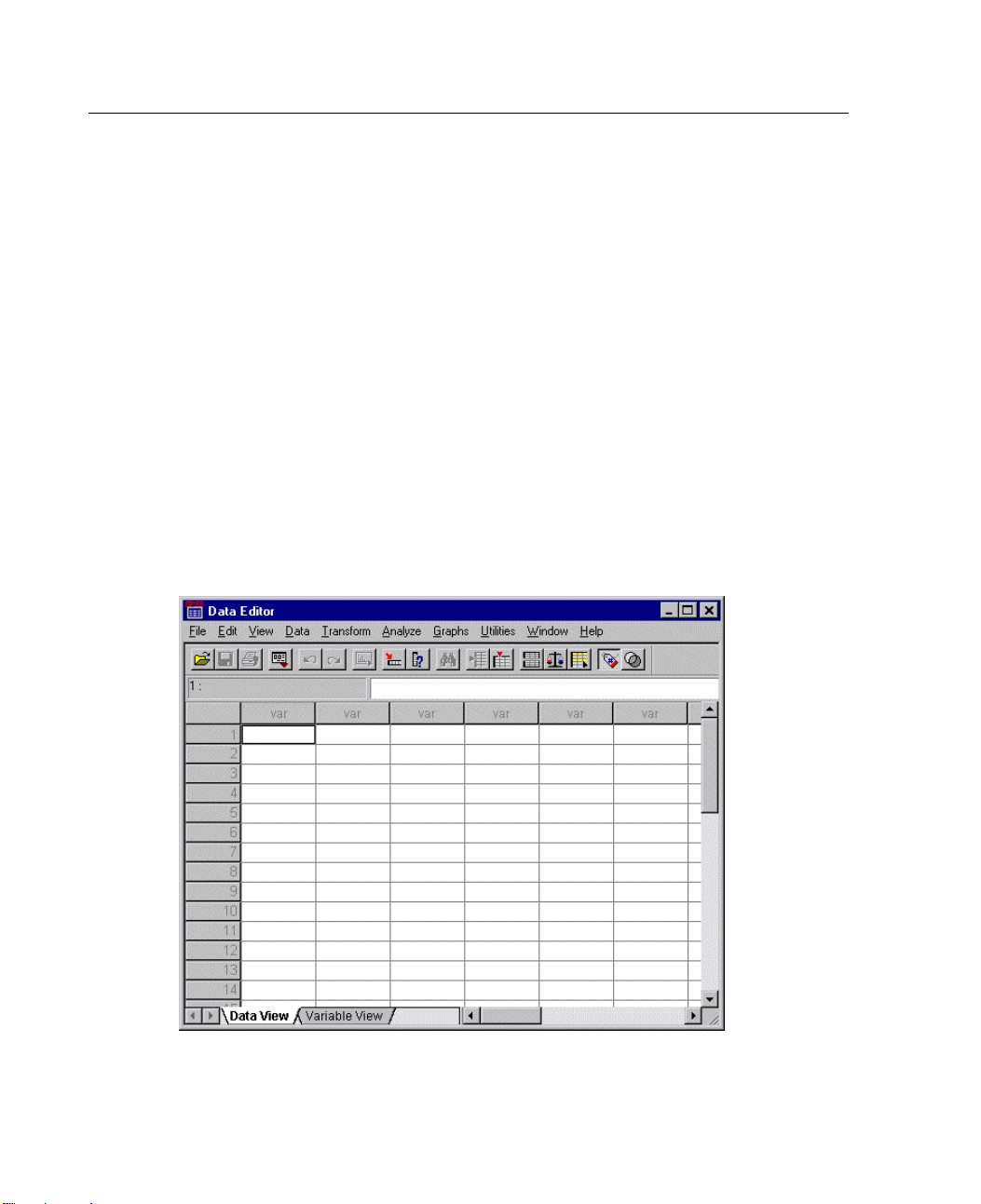
When you start a session, you see the Data Editor window.
Figure 1-1
Data Editor window (Data View)
S
S:
ndows Start menu choose:
Page 17

Variable Display in Dialog Boxes
Either variable names or longer variable labels will appear in list boxes in dialog
boxes. Additionally, variables in list boxes can be ordered alphabetically or by their
position in
In this guide, we will display variable labels in alphabetical order within list boxes.
For a new user of SPSS, this provides a more complete description of variables in
an easy-to-
Since the default setting within SPSS is to display variable labels in file order, we
will change this before accessing data.
E From the menus choose:
Edit
Options..
the file.
follow order.
.
3
Introduction
E
Select Dis
E Also selec
E Click OK,a
play labels
Alphabetical.
t
nd then click
Opening a Data File
Before you can analyze data, you need some data to analyze.
To open a data file:
E From the menus choose:
File
Open
Data...
in the Variable Lists group on the General tab.
OK to confirm the change.
Page 18
4
Chapter 1
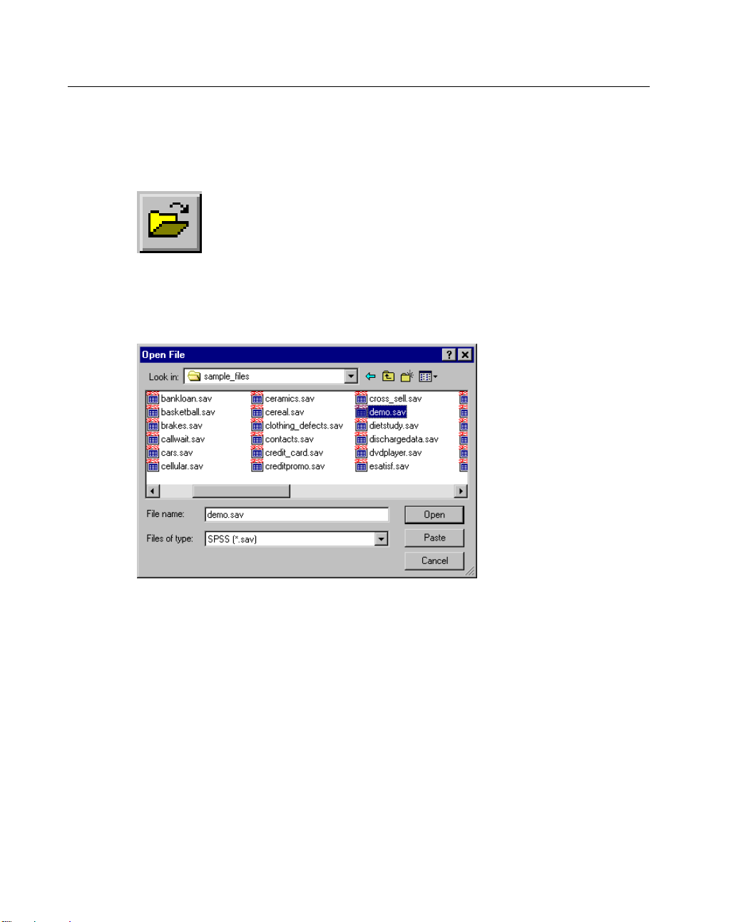
Alternatively, you can use the Open File button on the toolbar.
Figure 1-2
Open File too
lbar button
This opens the Open File dialog box.
Figure 1-3
Open File di
alog box
By default, SPSS-format data files (.sav extension) are displayed. You can display
other file formats using the Files of Type drop-down list.
By default, data files in the folder (directory) in which SPSS is installed are
displayed. The files for this guide are located in the folder in which SPSS is installed
or in the tutorial\sample_files folder within the SPSS installation folder.
E Double-click the tutorial folder.
E Double-click the sample_files folder.
E Click the file demo.sav in the files list box (or just demo if file extensions are not
displayed).
Page 19
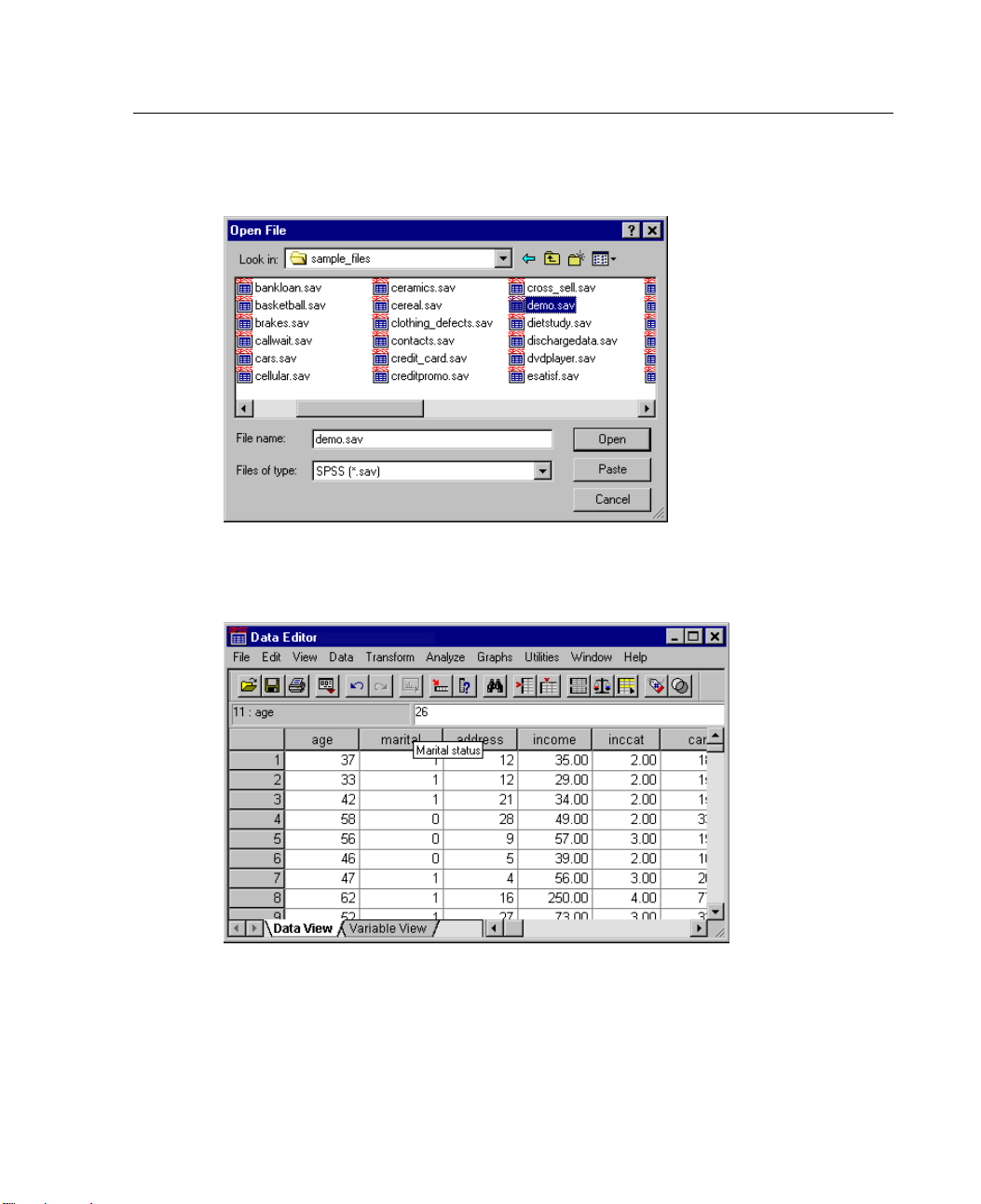
Figure 1-4
Sample_files folder displayed in Open File dialog box
E ClickOpentoopentheSPSSdatafile.
Figure 1-5
Variable labels
5
Introduction
ThedatafileisdisplayedintheDataEditor.Ifyouputthemousecursoronavariable
the column headings), a more descriptive variable label is displayed if one has
name (
been defined for that variable.
Page 20
6
Chapter 1
By default, the actual d ata values are displayed. To display labels:
E From the menus choose:
View
Value Labels
Alternatively, you can use the Label tool on the toolbar.
Figure 1-6
Value Labels
tool
Descriptive value labels are now displayed. This makes it easier to interpret the
responses.
Figure 1-7
Value labels displayed in the Data Editor
Page 21
Introduction
7
Running an An
The Analyze
categories. Most of the categories are followed by an arrow, which indicates that there
are several analysis procedures available within the category; they will appear on a
submenu whe
We’ll start with a simple frequency table (table of counts).
E From the menus choose:
Analyze
Descriptive Statistics
Frequencies...
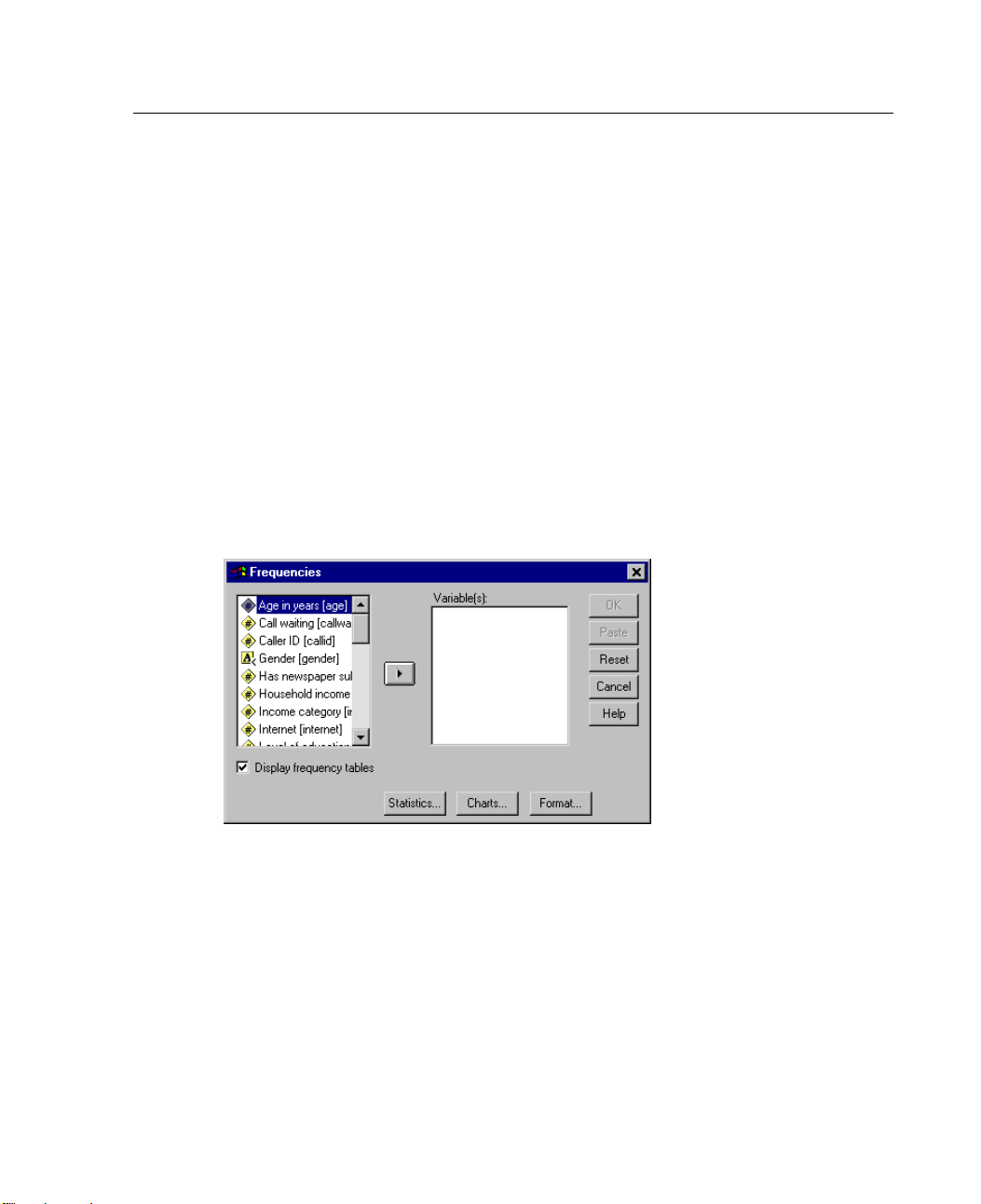
This opens the Frequencies dialog box.
Figure 1-8
Frequencies dialog box
alysis
menu contains a list of general reporting and statistical analysis
n the category is selected.
Page 22
8
Chapter 1
E
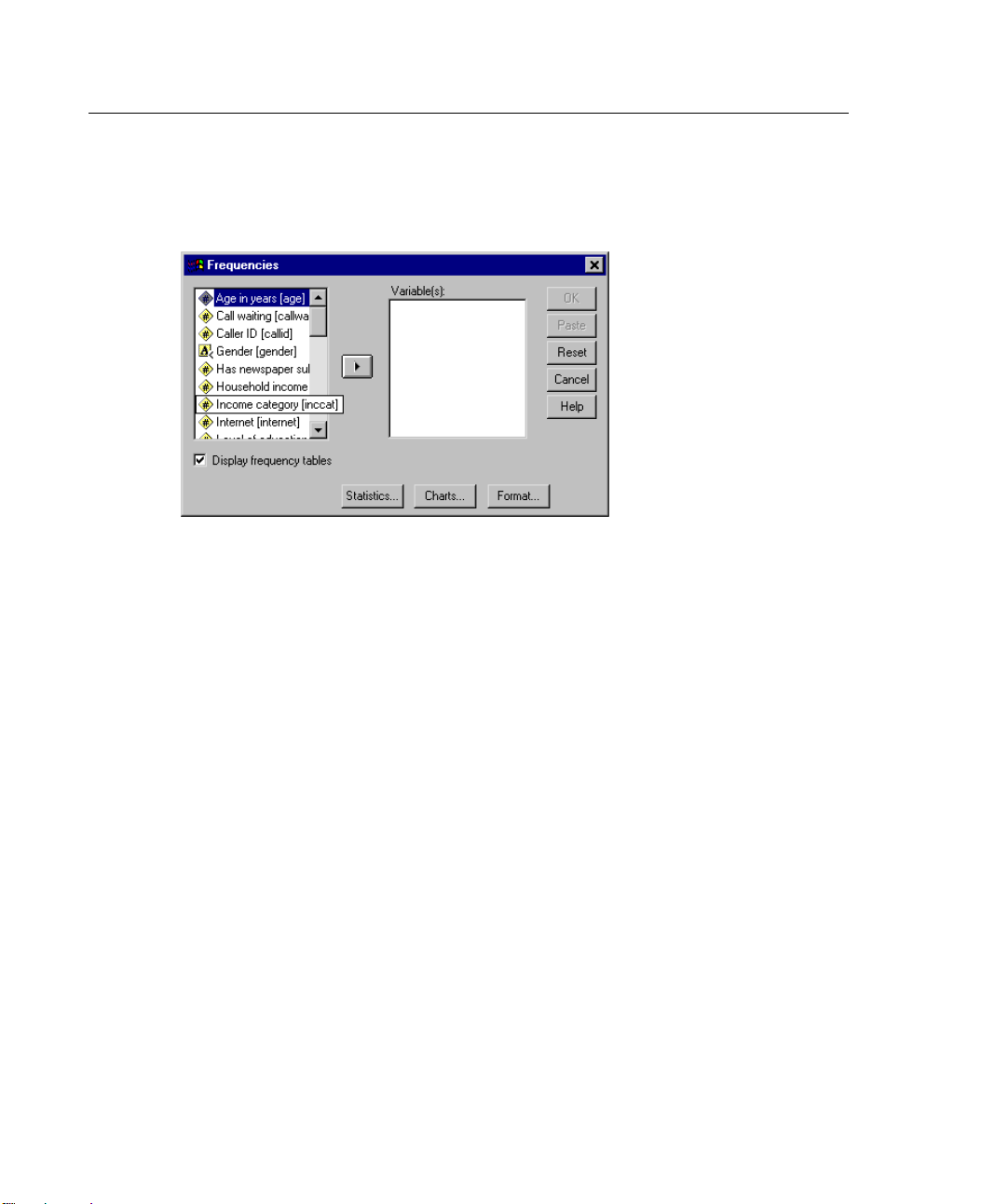
Select (click) the variable Income category.
Figure 1-9
Variable lab
els and names in the Frequencies dialog box
A more complete description of each variable pops up when the cursor is over it. The
variable name (in square brackets) is inccat, and it has the variable label Income
category
. If there were no variable label, only the variable name would appear in
the list box.
In the d ialog box, you choose the variables you want to analyze from the source list
on the le
ft and move them into the Variable(s) list on the right. The
OK button, which
runs the analysis, is disabled until at least one variable is placed in the Variable(s) list.
Additional labeling information can be easily obtained for any variable on the list
by click
ing on the variable name with the right mouse button.
E Click t
E Click the down arrow on the Value Labels drop-down list.
he right mouse button on Income Category [inccat], and then click (left mouse
button)
Variable Information.
Page 23
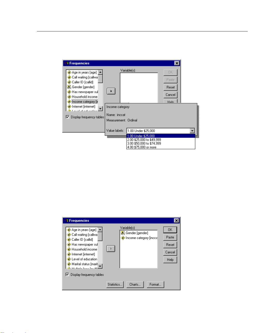
Figure 1-10
Defined labels for income variable
9
Introduction
All of the
E Click Ge
defined value labels for the variable are displayed.
nder [gender] in the source variable list, and then click the right-arrow
button to move the variable into the target Variable(s) list.
E Click Income category [inccat] in the source list, and then click the right arrow
button again.
Figure 1-11
Variables selected for analysis
Page 24
10
Chapter 1
A pound sign (#) icon next to the variablename indicates that the variable is numeric.
An icon with the letter “A” indicates that the variable is a string (alphanumeric)
variable, w
hich may contain both letters and numbers. A less-than sign (left angle
bracket) indicates that the variable is a short string, containing eight or fewer
characters.
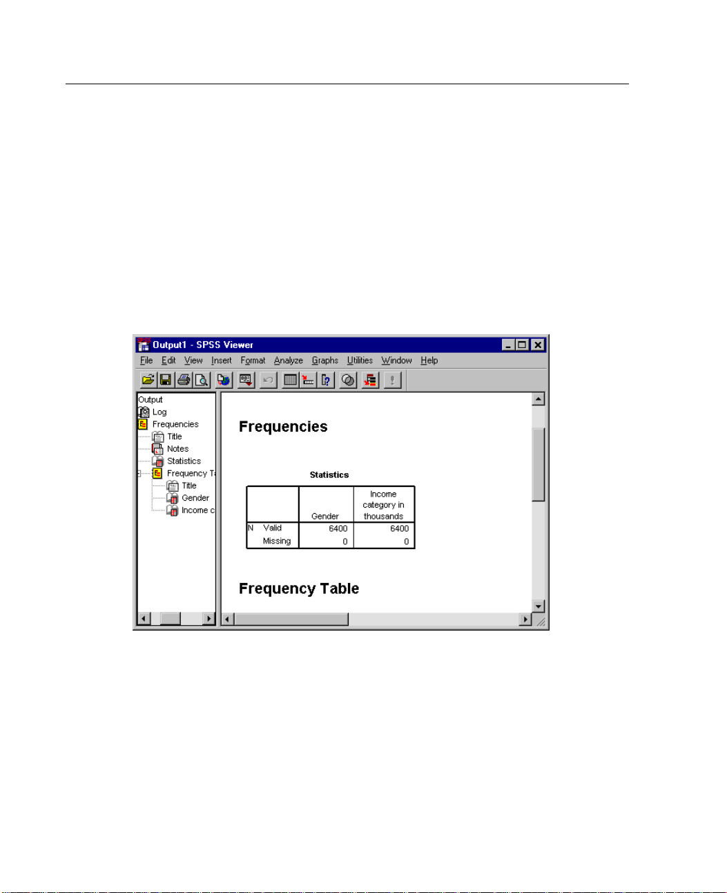
E Click OK to run the procedure.
Viewing Results
Figure 1-1
Viewer win
2
dow
Results are displayed in the Viewer window.
You can quickly go to any item in the Viewer simply by selecting it in the outline pane.
E Click Income category.
Page 25
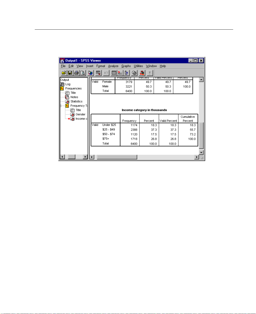
Figure 1-13
Frequency table of income categories
11
Introduction
Creati
kes you directly to the frequency table for income categories. This frequency
This ta
table shows the number and percentage of people in each income category.
ng Charts
gh some statistical procedures can create high-resolution charts, you can also
Althou
use the Graphs menu to create charts.
For example, you could create a chart that shows the relationship between wireless
one service and PDA (personal digital assistant) ownership.
teleph
E From t
E
he menus choose:
Graphs
Bar...
Click Clustered and then click Define.
Page 26
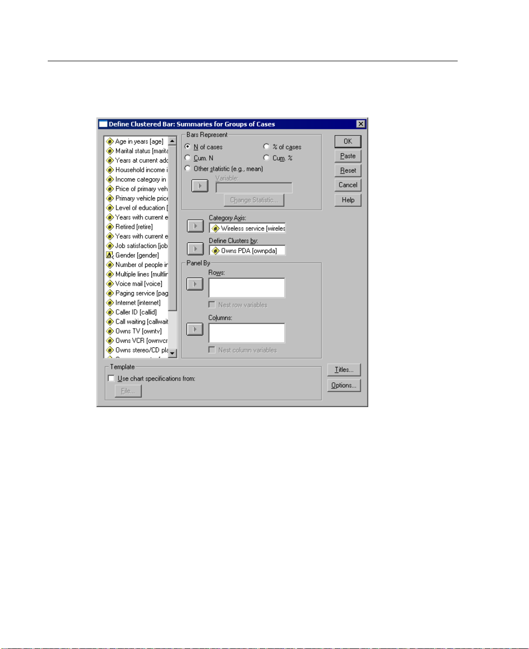
12
Chapter 1
Figure 1-14
Define Clustered Bar dialog box
E Scro
ll down the source variable list and select Wireless service [wireless] as the
Category Axis variable.
E Select Owns PDA [ownpda] as the Define Clusters By variable.
E Click OK to create the chart.
Page 27
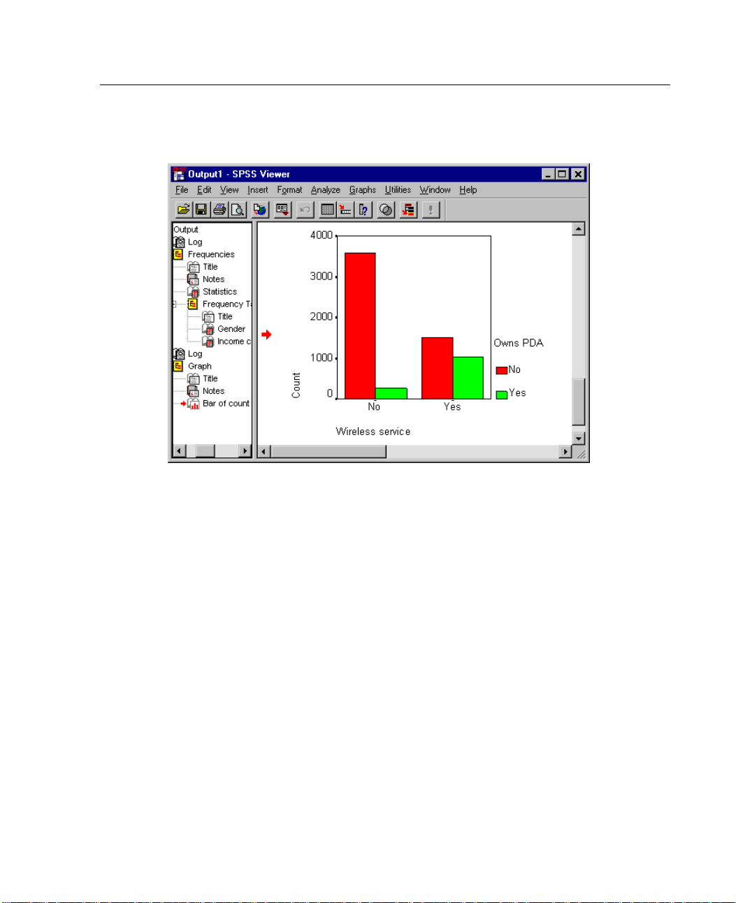
Figure 1-15
Bar chart displayed in Viewer window
13
Introduction
Exitin
The bar
chart is displayed in the Viewer. It shows that people with wireless phone
service are far more likely to have PDAs than people without wireless service.
You can edit charts and tables by double-clicking on them in the contents pane of
the View
er window, and you can copy and paste your results into other applications.
Those topics will be covered later.
g SPSS
To exit
E From t
File
E
Click No if you get an alert asking if you want to save your results.
SPSS:
he menus choose:
Exit
Page 28

Page 29

Chapter
2
Using the Hel
Help is available in a number of different ways, including:
Help menu. EverywindowhasaHelpmenuonthemenubar.TheTopicsmenuitem
provides a
find topics. The Tutorial menu item provides access to the introductory tutorial.
Dialog box Help buttons. Most dialog boxes have a Help button that takes you directly
to a Help to
links to related topics.
Pivot table context menu Help. Right-click on terms in an activated pivot table in
the Viewe
of the terms.
Statistics Coach. The Statistics Coach item on the Help menu provides a wizard-like
method fo
ccess to the Help system, where you can use the Contents and Index tabs to
pic for that dialog box. The Help topic provides general information and
randselect
r finding the right statistical or charting procedure for what you want to do.
What’s This? from the context menu to display definitions
p System
Case Studies. The Case Studies item on the Help menu provides hands-on examples
of how to create various types of statistical analyses and interpret the results. The
sample d
the examples to see exactly how the results were produced.
This chapter uses the files demo.sav and bhelptut.spo.
ata files used in the examples are also provided so that you can work through
15
Page 30
16
Chapter 2
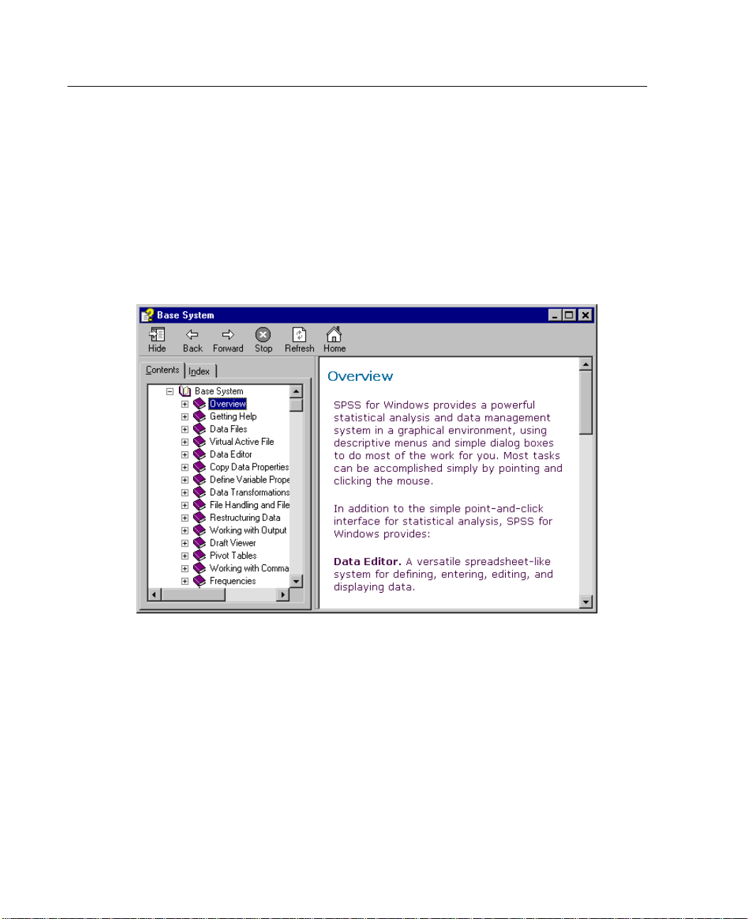
Help Content
The Topics i
E From the men
Help
Topics
Figure 2-1
Help Cont ent
sTab
tem on the Help menu opens a Help window.
us choose:
stab
The Contents tab in the left pane of the Help window is an expandable and collapsible
table of contents. It is most useful if you’re looking for general information or are
unsure of what index term to use to find what you’re looking for.
Page 31
17
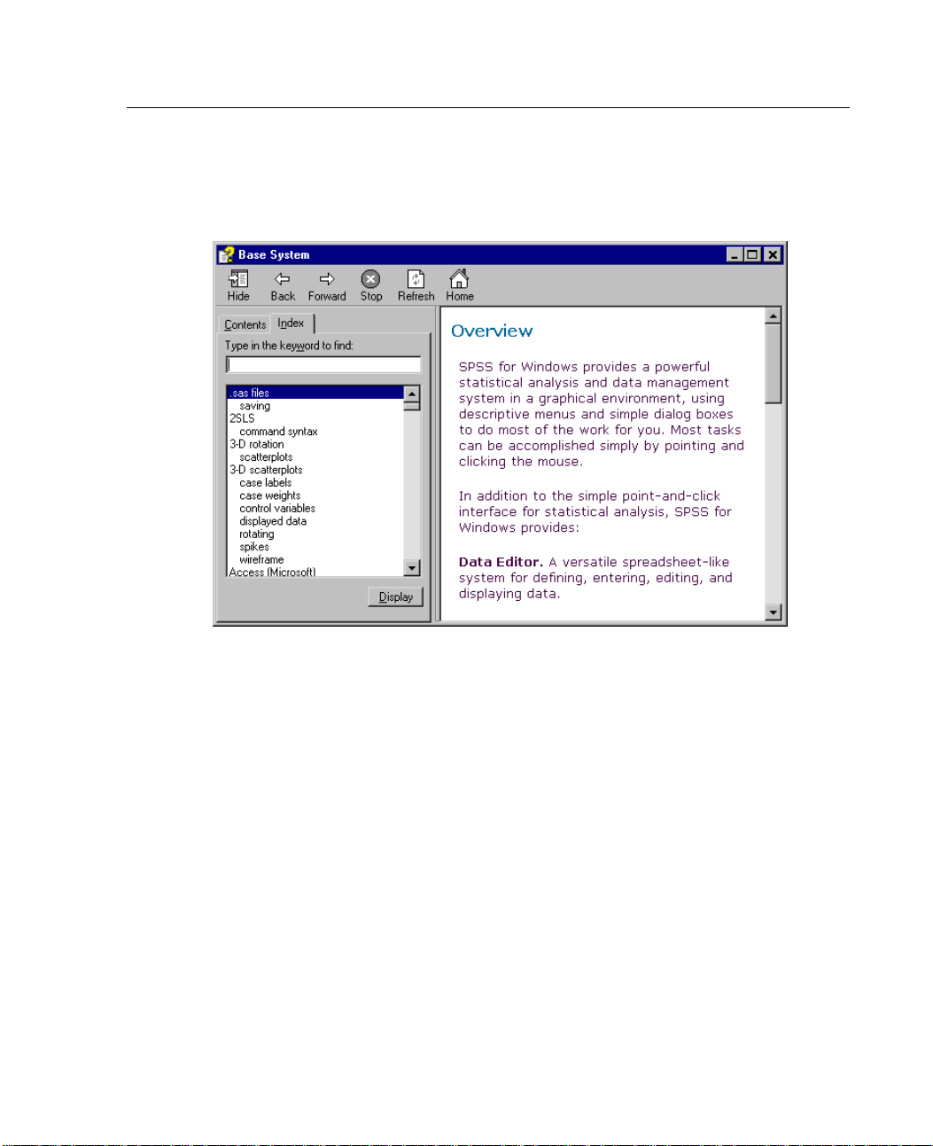
Help Index Ta
Figure 2-2
Help Index tab
Using the Help S
ystem
b
E Click the Index tab in the left pane of the Help window.
The Ind
The Index tab is organized in alphabetical order, just like a book index. It uses
incremental search to find what you’re looking for.
ex tab provides a searchable index that makes it easy to find specific topics.
Page 32
18
Chapter 2
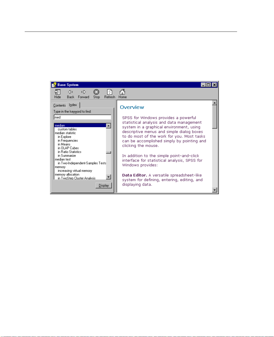
For example, you can:
E Type med.
Figure 2-3
Incremental
index search
The index scrolls to and highlights the first index entry that starts with these letters,
which is median.
Dialog Box Help
Most dialog boxes have a H elp button that displays a Help topic about what the
dialog box does and how to do it.
E From the menus choose:
Analyze
Descriptive Statistics
Frequencies...
Page 33
19
E
Click Help.
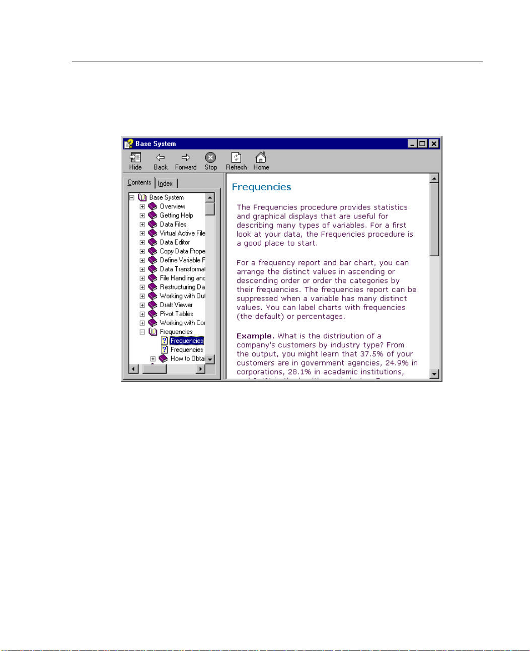
Figure 2-4
Dialog box He
lp topic
Using the Help S
ystem
In this example, the Help topic describes the purpose of the Frequencies procedure
andprovidesanexample.
Statistics Coach
The Statistics Coach can help to guide you through the process of finding the
procedure that you want to use.
E From the menus choose:
Help
Statistics Coach
Page 34
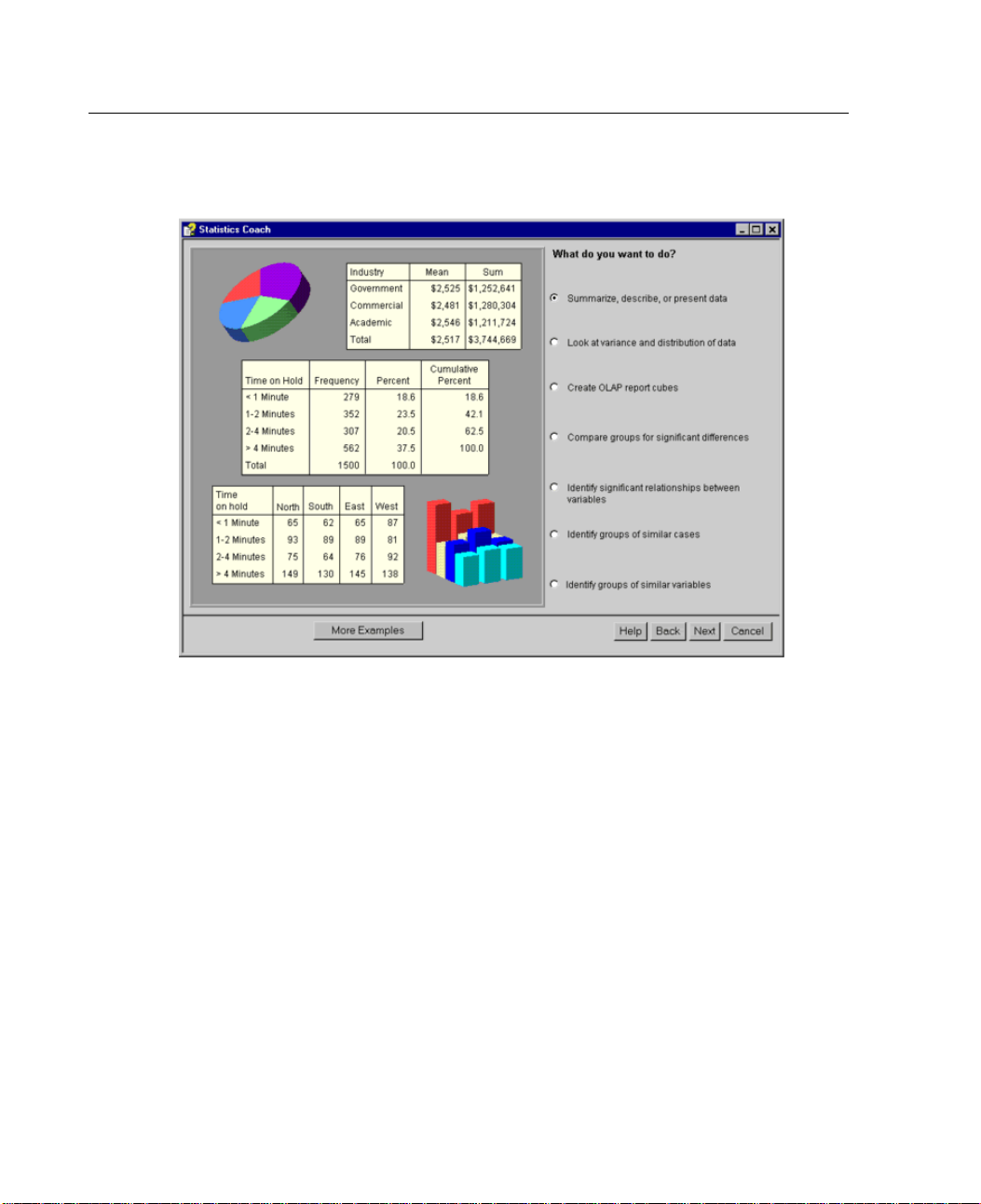
20
Chapter 2
Figure 2-5
Statistics Coach, first step
The Statistics Coach presents a series of questions designed to find the appropriate
procedure. The first question is simply “What do you want to do?”
For example, if you want to summarize data:
E Select Summarize, describe, or present data.
E Then click Next.
Page 35
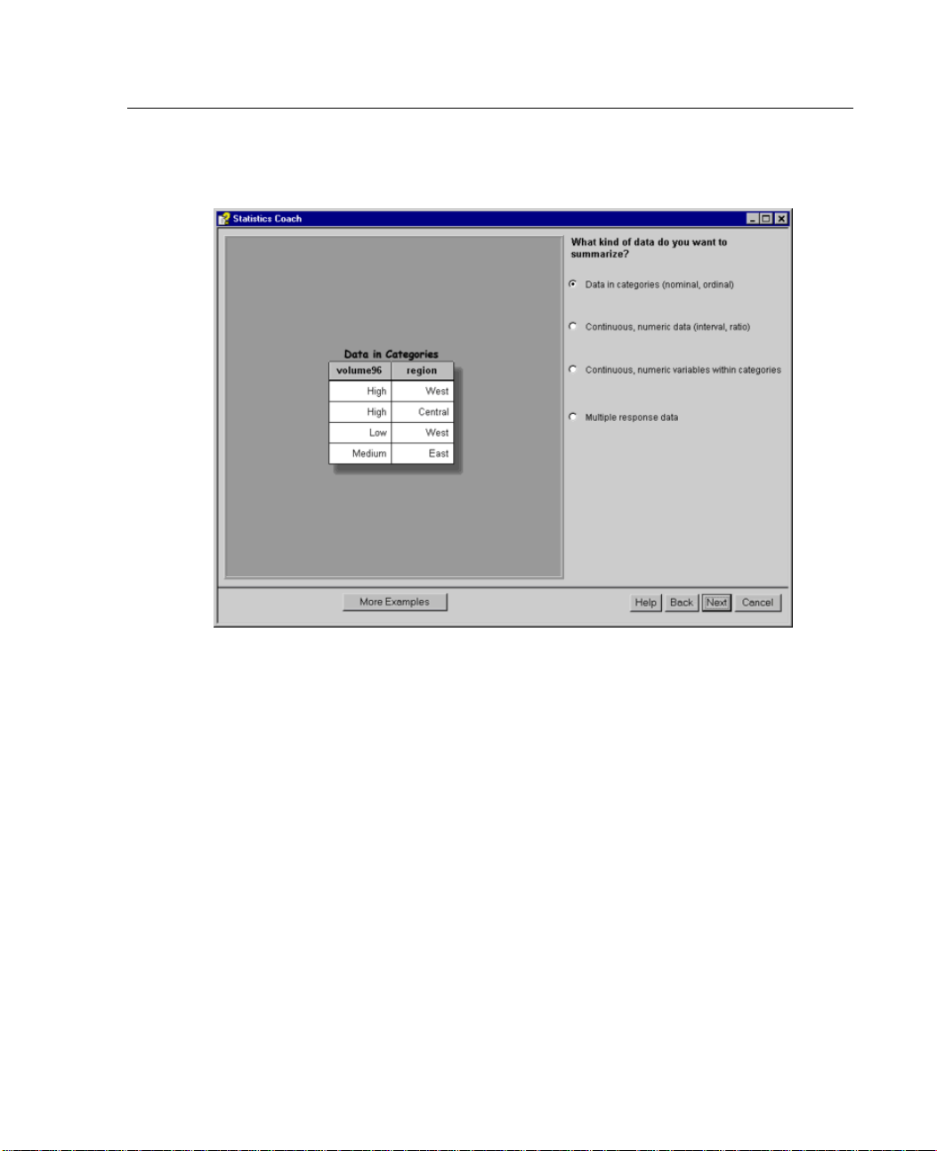
21
Figure 2-6
Data type selection
Using the Help S
ystem
The next question asks about the type of data you want to summarize. If you’re
unsure, each choice displays different examples.
E Select Continuous, numeric data (interval, ratio).
Page 36
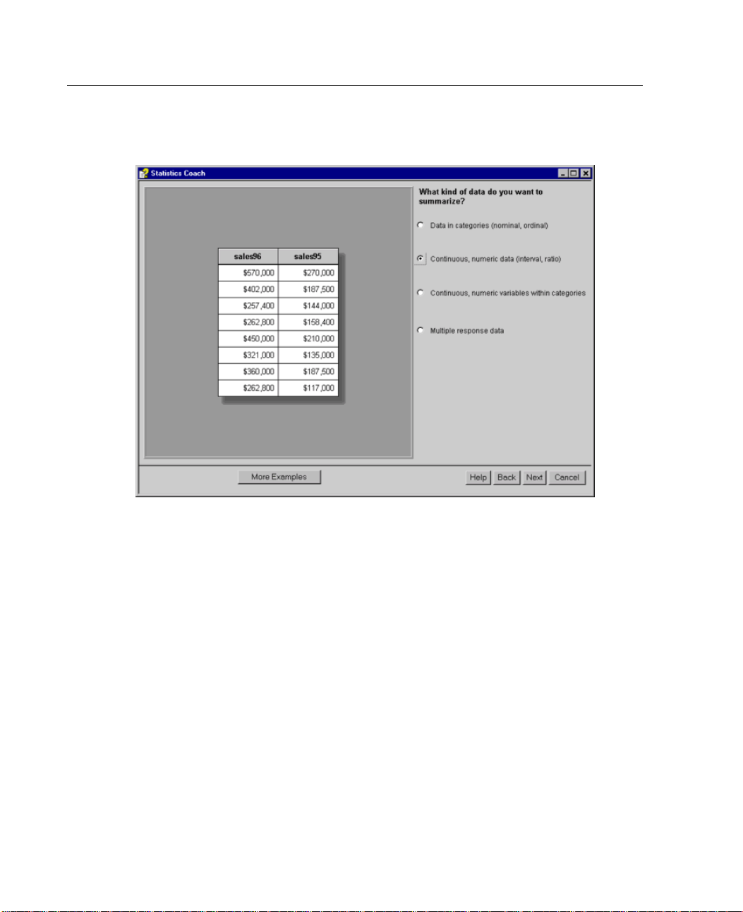
22
Chapter 2
Figure 2-7
Selecting a different data type
The example changes to reflect your choice. If you’re still unsure, you can:
E Click More Examples.
A new example of the same data type is displayed. If the examples don’t provide
enough information, you can:
E Click Help.
Page 37
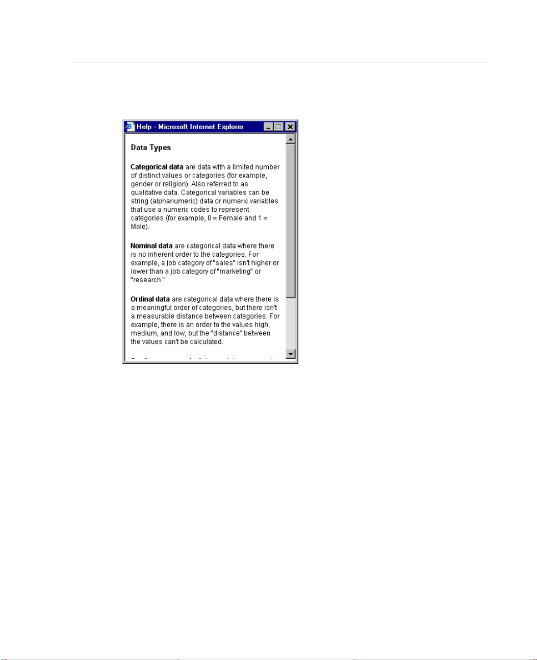
23
Figure 2-8
Statistics Coach Help topic
Using the Help S
ystem
In this example, the Help topic defines the different data types.
E Close the Help window.
E Select Data in categories (nominal, ordinal) and click Next.
Page 38
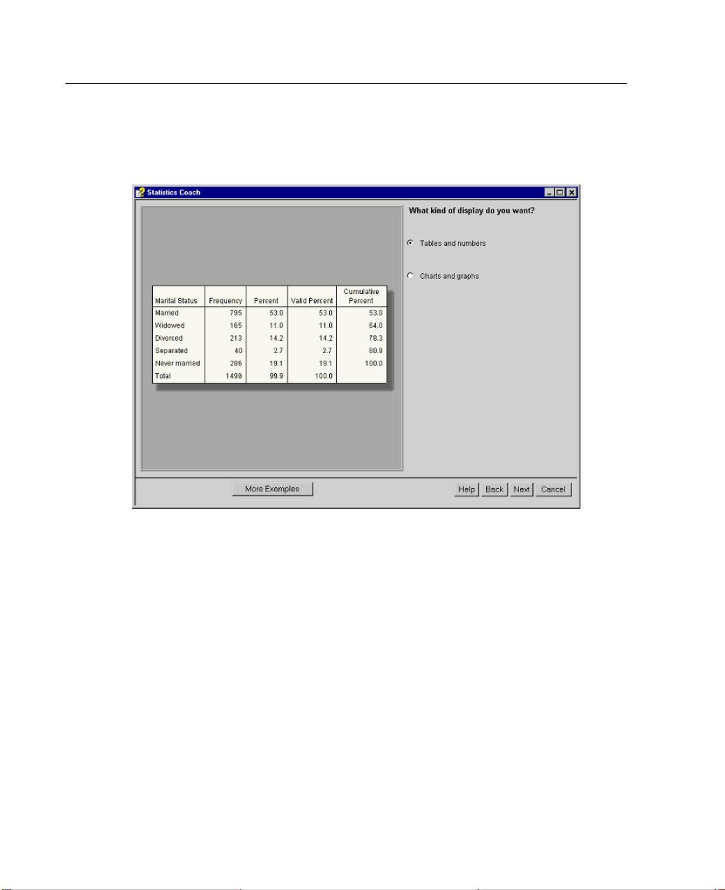
24
Chapter 2
E
Select Tables and numbers and click Next.
Figure 2-9
Selecting ta
bles or charts
Page 39
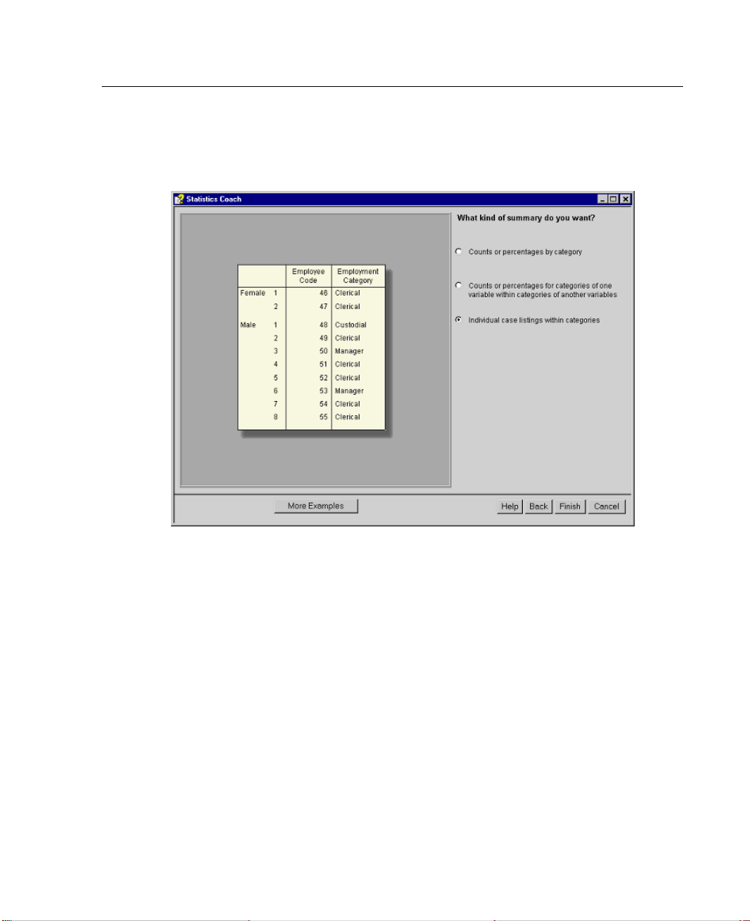
25
E
Select Individual case listings within categories.
Figure 2-10
Statistics C
oach, final step
Using the Help S
ystem
When th
e Statistics Coach has enough information, the
Next button changes to Finish.
Page 40
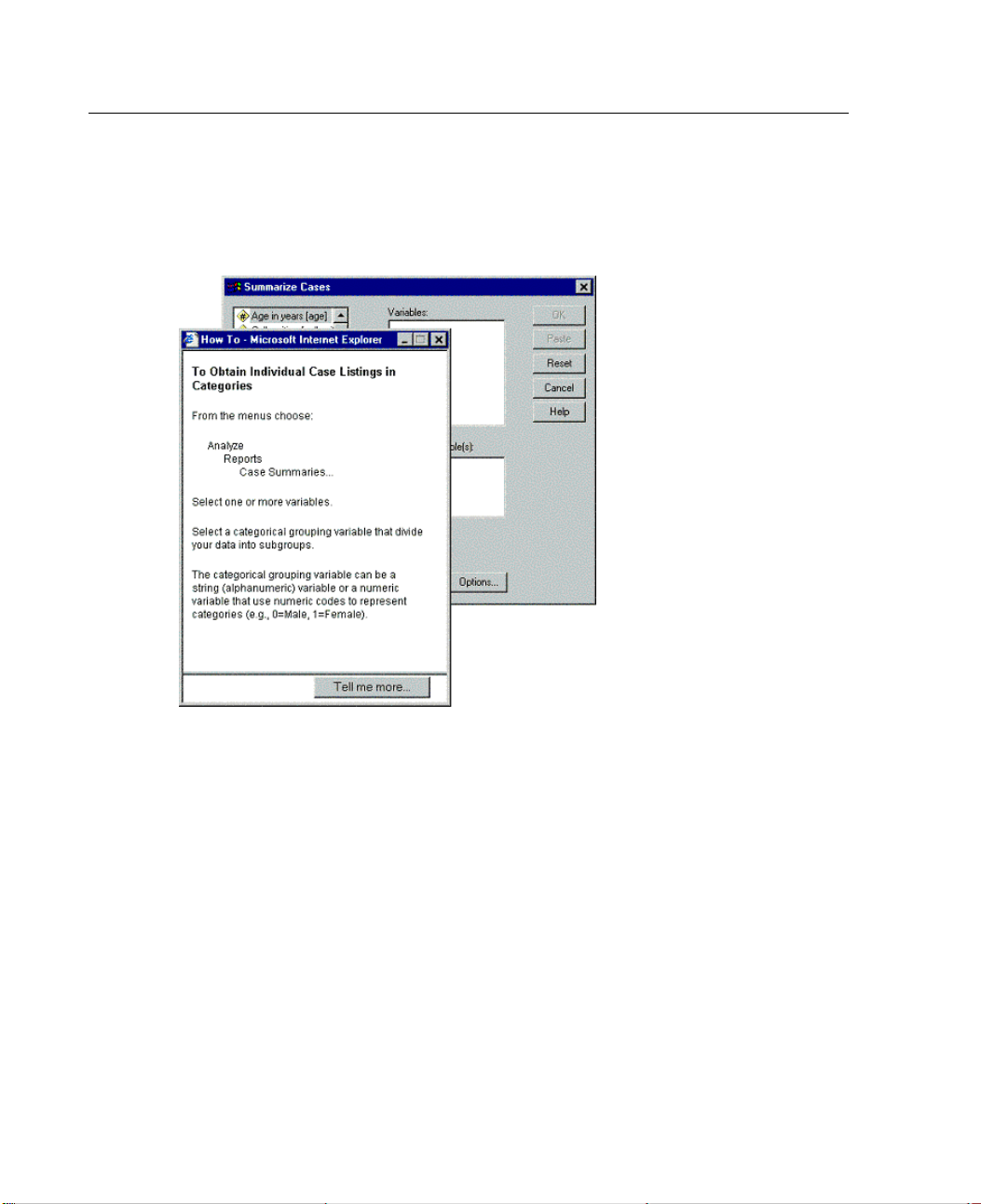
26
Chapter 2
When you click Finish, the dialog box for the selected procedure opens
automatically, and a Help topic for the procedure is also displayed.
Figure 2-11
Dialog box and Help topic
This is a custom Help topic, based on your selections in the Statistics Coach. Since
some dialog boxes perform numerous functions, more than one path in the Statistics
Coach may lead to the same dialog box, but the instructions in the Help topic may
be different.
E Click Tell me more in the Help topic to get more detailed information.
Page 41
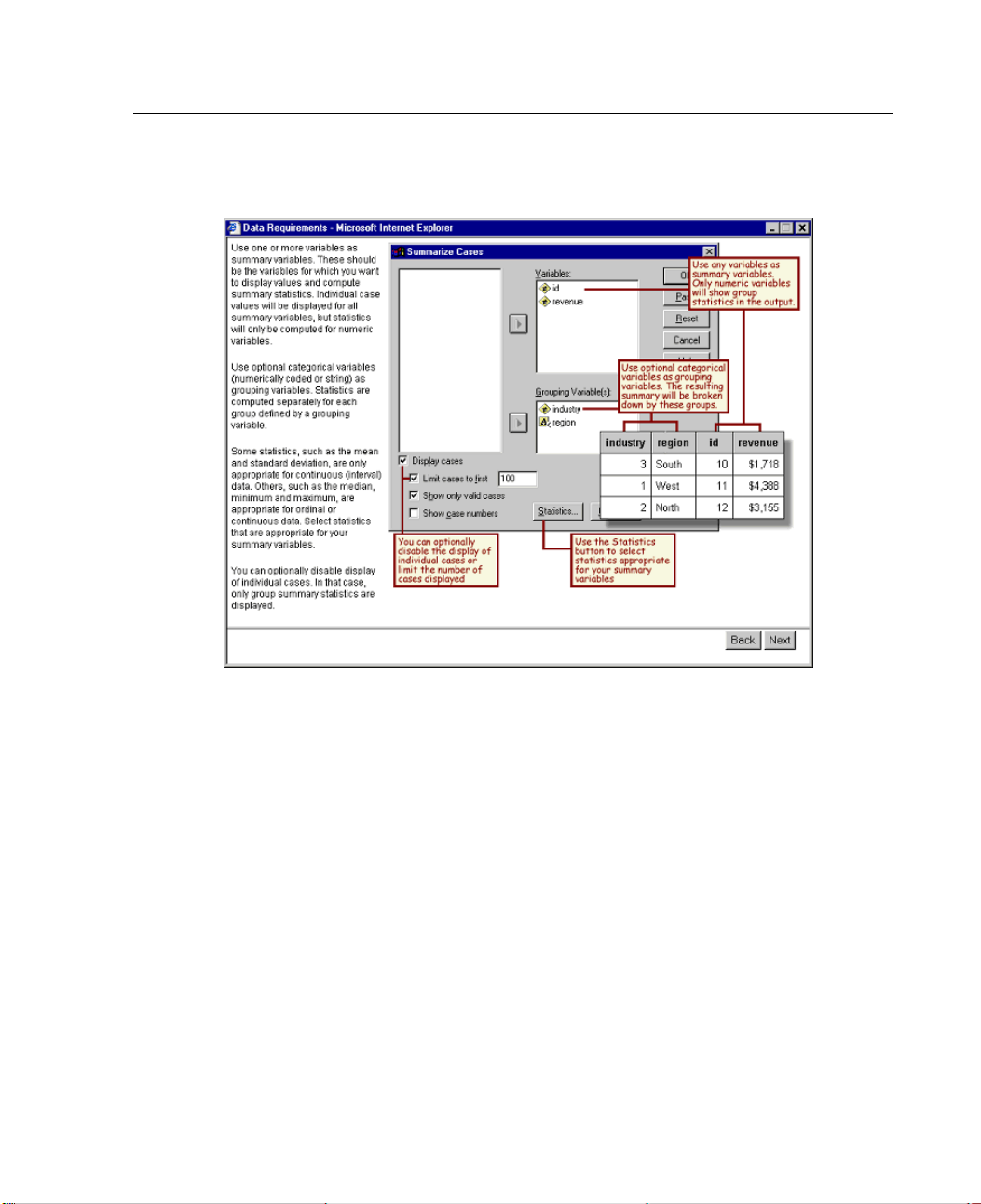
27
Figure 2-12
“Tell me m ore” Help topic
Using the Help S
ystem
Case St
E Righ
This He
the selected procedure.
lp topic provides detailed information on the data type(s) appropriate for
udies
Case st
in the examples are installed with SPSS, so you can follow along, performing the
same analysis—from opening the data source and selecting variables for analysis to
inter
To acc
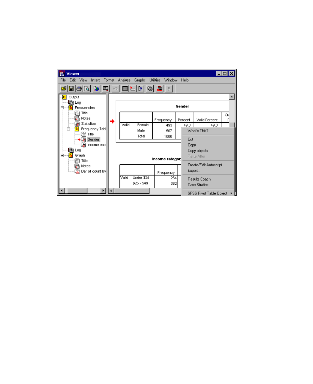
right-click on the frequency table for Gender.
udies provide comprehensive overviews of each procedure. Data files used
preting the results.
ess the case studies:
t-click on any pivot table created by a procedure. For example, you can
Page 42
28
Chapter 2
Figure 2-13
Accessing the case studies
E Select Case Studies on the pop-up context menu.
Case studies are not available for all procedures. The Case Studies choice on the
context menu will appear only if the feature is available for the procedure that created
the selected pivot table.
Page 43
Reading Data
Data can be entered directly into SPSS, or it can be imported from a number
of differen
spreadsheet applications, such as Microsoft Excel, database applications, such as
Microsoft Access, and text files are all discussed in this chapter.
Basic Structure of an SPSS Data File
t sources. The processes for reading data stored in SPSS data files,
Chapter
3
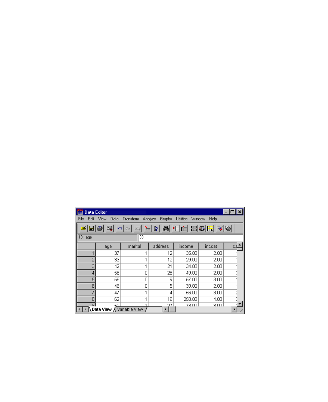
Figure 3-1
Data Edito
SPSS data files are organized by cases (rows) and variables (columns). In this data
file, cases represent individual respondents to a survey. Variables represent each
question asked in the survey.
r
29
Page 44
30
Chapter 3
ReadinganSP
SPSS data fi
demo.sav, an example file that is installed with the product:
E From the menus choose:
File
Open
Data...
Make sure that SPSS (*.sav) is selected in the Files of Type drop-down list.
E
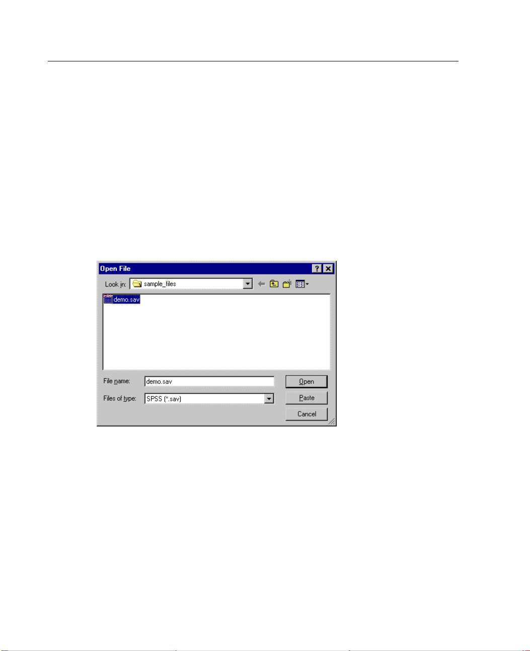
Figure 3-2
Open File dialog box
SS Data File
les, which have a .sav file extension, contain your saved data. To open
E Navigate to the sample_files folder.
E Select demo.sav and click Open.
Page 45
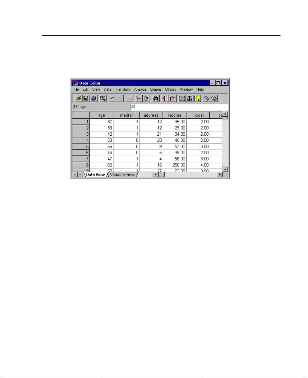
The data are now displayed in the Data Editor.
31
Reading Data
Figure 3-3
Opened data f
ile
Reading Data from Spreadsheets
Rather than typing all of your data directly into the Data Editor, you can read data
from applications such as Microsoft Excel. You can also read column headings
as variable names.
E From the menus choose:
File
Open
Data...
Page 46
32
Chapter 3
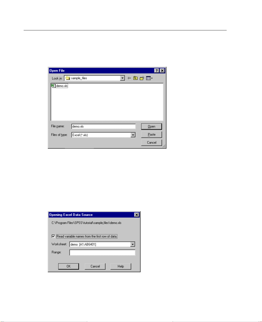
E
Select Excel (*.xls) from the Files of Type drop-down list.
Figure 3-4
Open File dia
E Select demo.xls and click Open to read this spreadsheet.
log box
The Opening Excel Data Source dialog box is displayed, allowing you to specify
whether variable names are to be included in the spreadsheet, as well as the cells that
you want to import. In Excel 5 or later, you can also specify which worksheets
youwanttoimport.
Figure 3-5
Opening Excel Data Source dialog box
Page 47
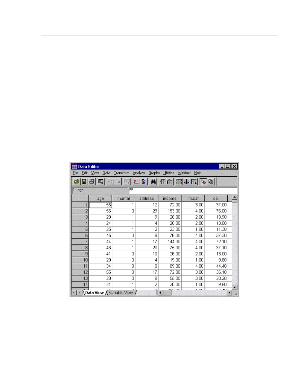
E
Make sure that Read variable names from f irst row of data is selected. This option
reads column headings as variable names.
33
Reading Data
If the column
headings do not conform to the SPSS variable-naming rules, they are
converted into valid variable names and the original column headings are saved as
variable labels. If you want to import only a portion of the spreadsheet, specify the
range of cel
E Click OK to
Thedatanow
ls to be imported in the Range text box.
read the Excel file.
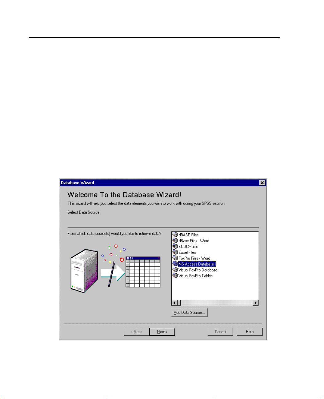
appear in the Data Editor, with the column headings used as variable
names. If you’re using a spreadsheet application other than Excel or Lotus, you should
be able to export your data to a supported format that can then be read into SPSS.
Figure 3-6
Imported Excel data
Page 48
34
Chapter 3
Reading Data
Data from da
database that uses ODBC (Open Database Connectivity) drivers can be read directly
by SPSS after the drivers are installed. ODBC drivers for many database formats are
supplied on
vendors. One of the most common database applications, Microsoft Access, is
discussed in this example.
E From the menus choose:
File
Open Datab
New Query.
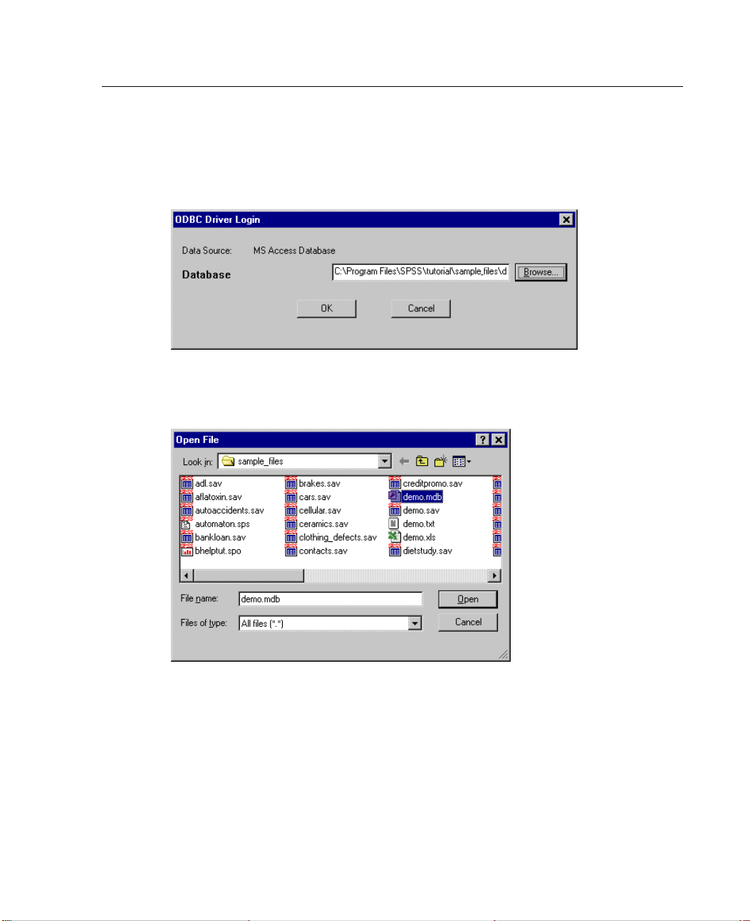
Figure 3-7
Database W izard Welcome dialog box
from a Database
tabase sources are easily imported using the Database Wizard. Any
the installation CD. Additional drivers can be obtained from third-party
ase
..
E Select MS Access Database from the list of data sources and click Next.
Page 49
Reading Data
If MS Access Database is not listed here, you need to run Microsoft Data Access
Pack.exe, which can be found in the Microsoft Data Access Pack folder on the CD.
Figure 3-8
ODBC Driver Login di alog box
E Click Browse to navigate to the Access database file that you want to open.
Figure 3-9
Open File dialog box
35
E Selec
E Click O
t demo.mdb and click
in the login dialog box.
K
Open to continue.
Page 50
36
Chapter 3
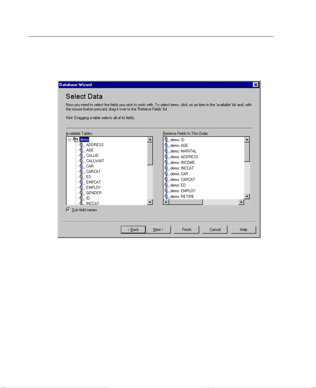
In the next step, you can specify the tables and variables that you want to import.
Figure 3-10
Select Data s
tep
E Drag the entire demo table to the Retrieve Fields in This Order list.
E Click Next.
Page 51
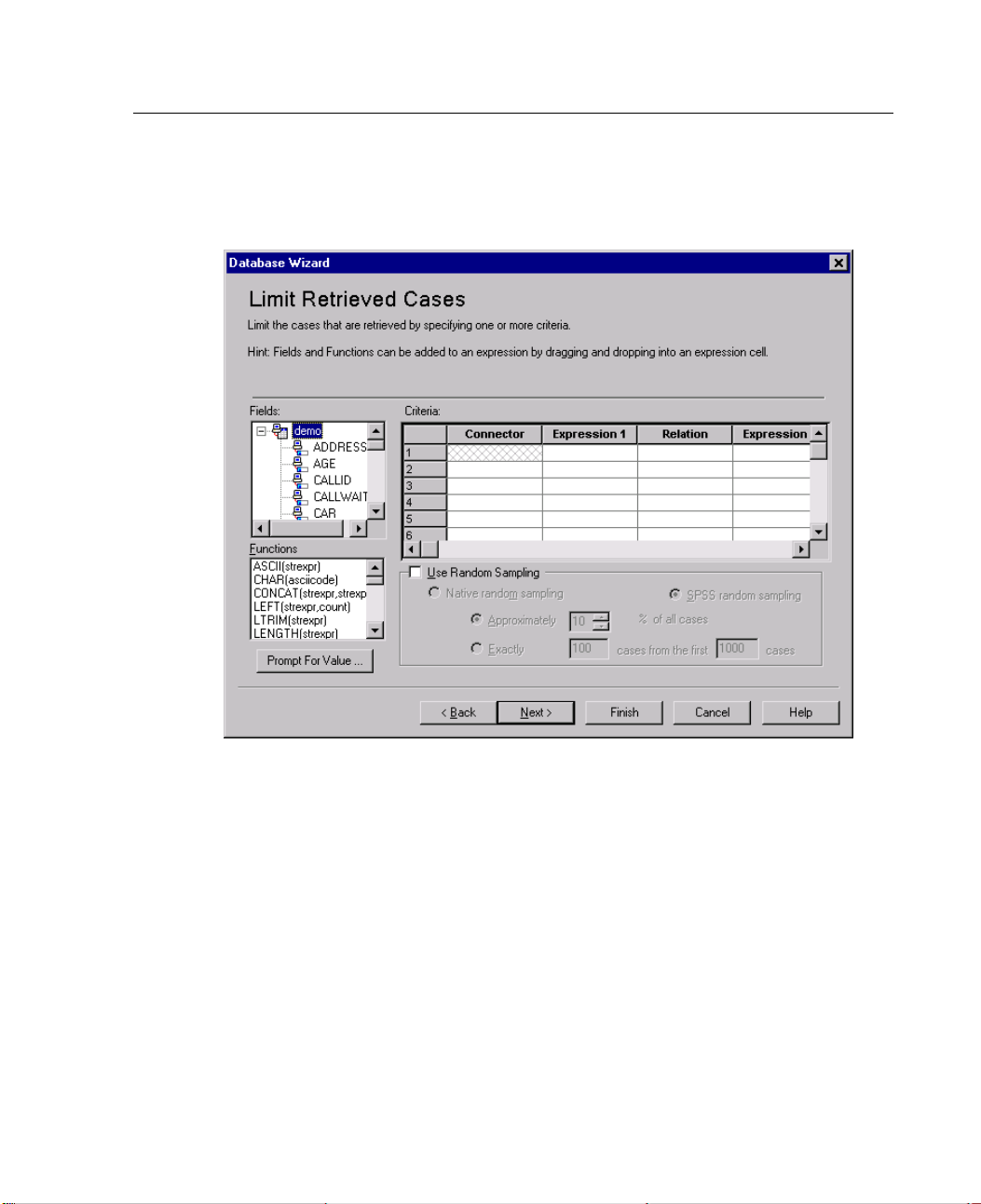
In the next step, you select which records (cases) to import.
37
Reading Data
Figure 3-11
Limit Retrie
ved Cases step
If you do not want to import all cases, you can import a subset of cases (for example,
males older than 30), or you can import a random sample of cases from the data
source. For large data sources, you may want to limit the number of cases to a small,
representative sample to reduce the processing time.
E Click Next to continue.
Page 52
38
Chapter 3
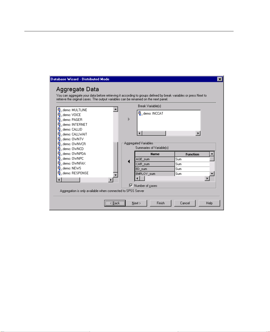
If you are in distributed mode, connected to a remote server (available with SPSS
Server), the next step allows you to aggregate the data before reading it into SPSS.
Figure 3-12
Aggregate Data step
You can also aggregate data after reading it into SPSS, but pre-aggregating may
save time for large data sources.
E For this example, you don’t need to aggregate the data. If you see this step in the
Database Wizard, click
Next.
Page 53
Reading Data
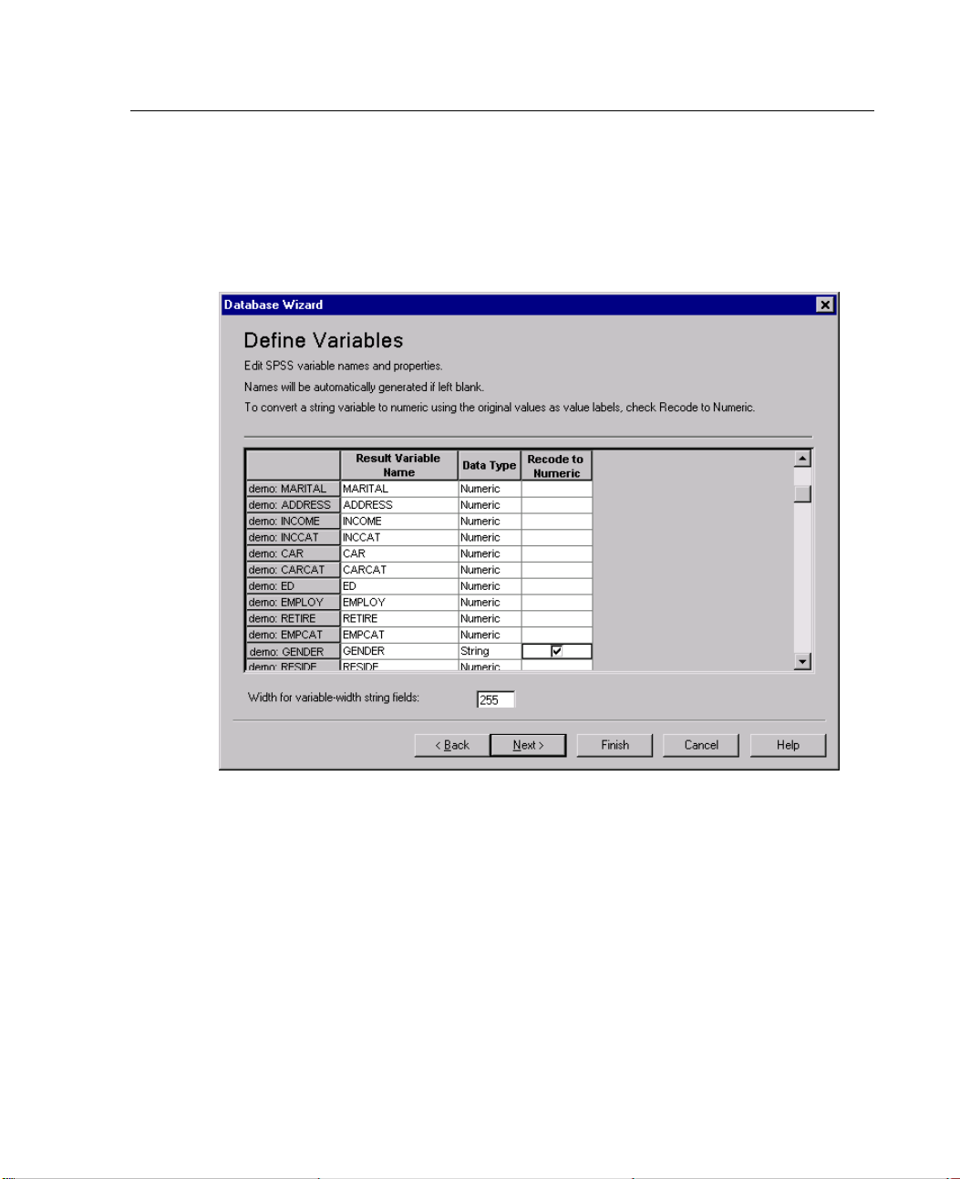
Field names are used to create variable names. If necessary, the names are converted
to valid variable names. The original field names are preserved as variable labels.
You can also
Figure 3-13
Define Variables step
change the variable names before importing the database.
39
E Click the Recode to Numeric cell in the Gender field. This option converts string
variables to integer variables and retains the original value as the value label for
the new variable.
E Click Next to continue.
If you are in distributed mode, connected to a remote server (available with SPSS
Server), the next step allows you sort the data before reading it into SPSS.
Page 54
40
Chapter 3
You can also sort data after reading it into SPSS, but presorting may save time for
largedatasources.
E For this example, you don’t need to sort the data. If you see this step in the Database
Next.
Wizard, cli
ck
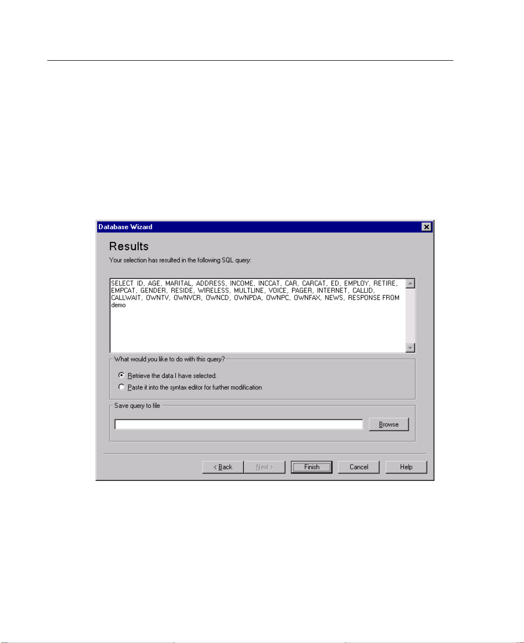
The SQL state
ment created from your selections in the Database Wizard appears in
the Results step. This statement can be executed now or saved to a file for later use.
Figure 3-14
Results ste
p
E Click Finish to import the data.
Page 55
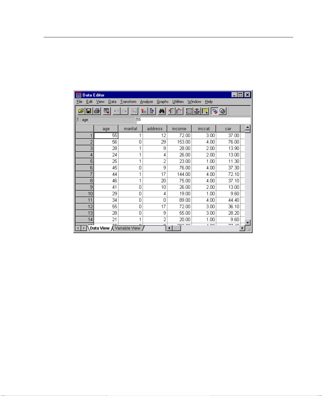
41
Reading Data
All of the data in the Access database that you selected to import are now available in
theSPSSDataEditor.
Figure 3-15
Data imported from an Access database
Readin
gDatafromaTextFile
les are another common source of data. Many spreadsheet programs and
Text fi
databases can save their contents in one of many text file formats. Comma or
tab-delimited files refer to rows of data that use commas or tabs to indicate each
ble. In this example, the data are tab delimited.
varia
Page 56
42
Chapter 3
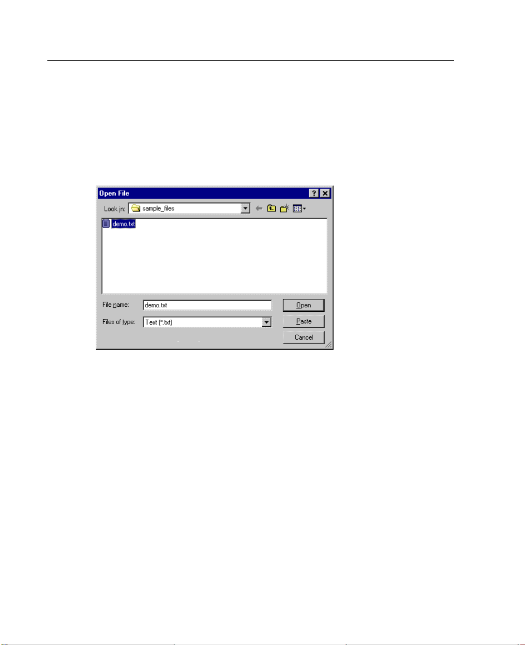
E
From the menus choose:
File
Read Text Data...
E
Choose Text (*.txt) from the Files of Type list.
Figure 3-16
Open File dialog box
E Select demo.txt and click Open to read the selected file.
Page 57
43
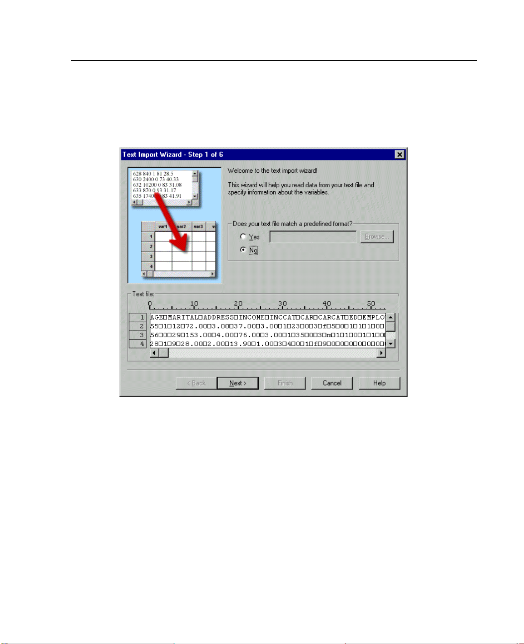
Reading Data
The Text Import Wizard guides you through the process of defining how the specified
text file should be interpreted.
Figure 3-17
Text Import Wizard - Step 1 of 6
E In Step 1, you can choose a predefined format or create a new format in the wizard.
Select No to indicate that a new format should be created.
E Click Next to continue.
Page 58
44
Chapter 3
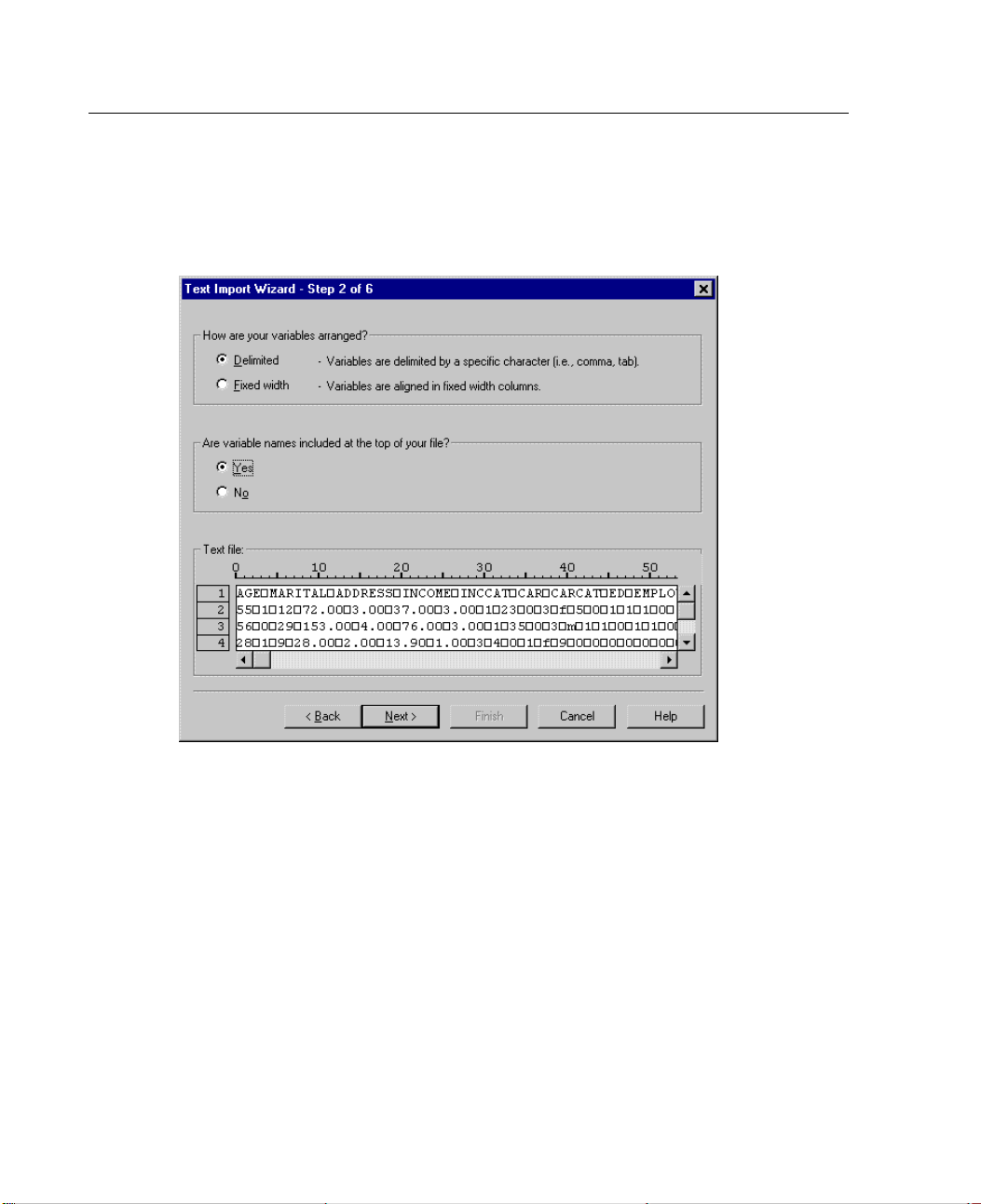
As stated earlier, this file uses tab-delimited formatting. Also, the variable names
aredefinedonthetoplineofthisfile.
Figure 3-18
Text Import Wizard - Step 2 of 6
E Select Delimited to indicate that the data use a delimited formatting structure.
E Select Yes to indicate that variable names should be read from the top of the file.
E Click Next to continue.
Page 59
E
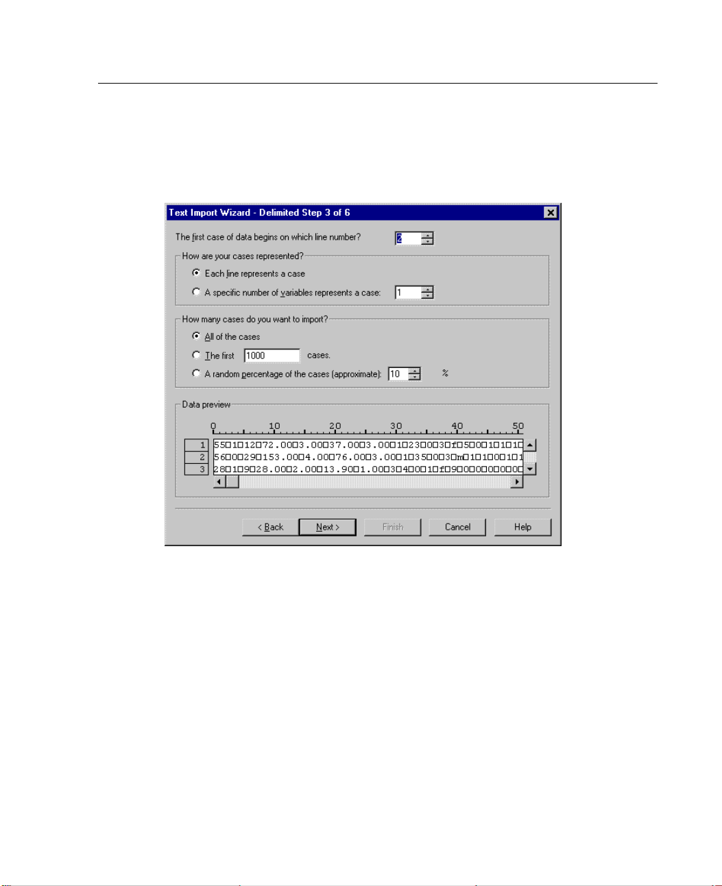
Type 2 in the top section of next dialog box to indicate that the first row of data
starts on the second line of the text file.
Figure 3-19
Text Import Wizard - Step 3 of 6
45
Reading Data
E Keepthe default values for the remainder of this dialog box, and click Next to continue.
Page 60
46
Chapter 3
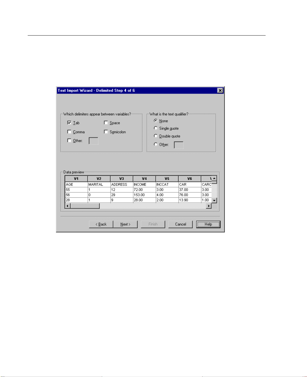
The Data preview in Step 4 provides you with a quick way to ensure that your data
are being properly read by SPSS.
Figure 3-20
Text Import Wizard - Step 4 of 6
E Select Tab and deselect the other options.
E Click Next to continue.
Page 61
47
Reading Data
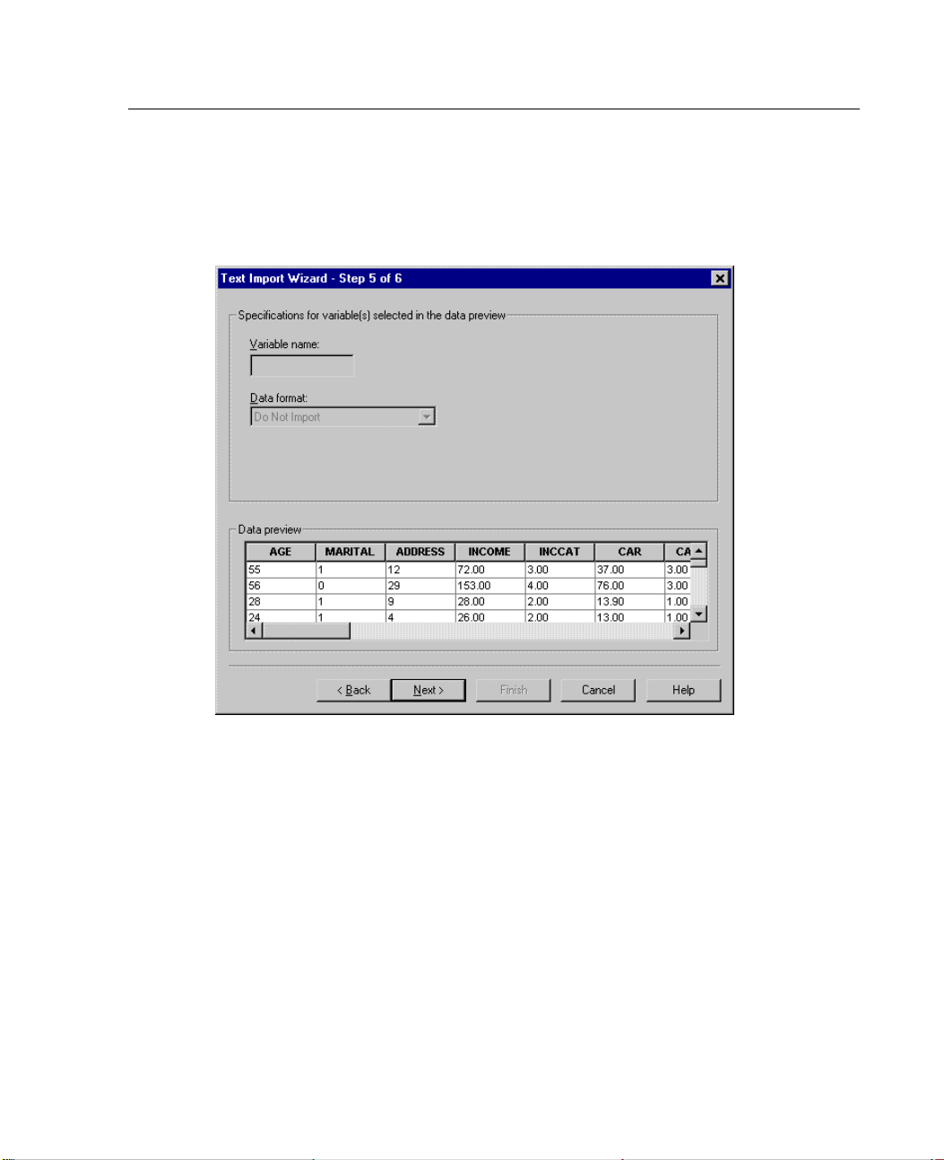
Because the variable names may have been truncated to fit SPSS formatting
requirements, this dialog box gives you the opportunity to edit any undesirable names.
Figure 3-21
Text Import Wizard - Step 5 of 6
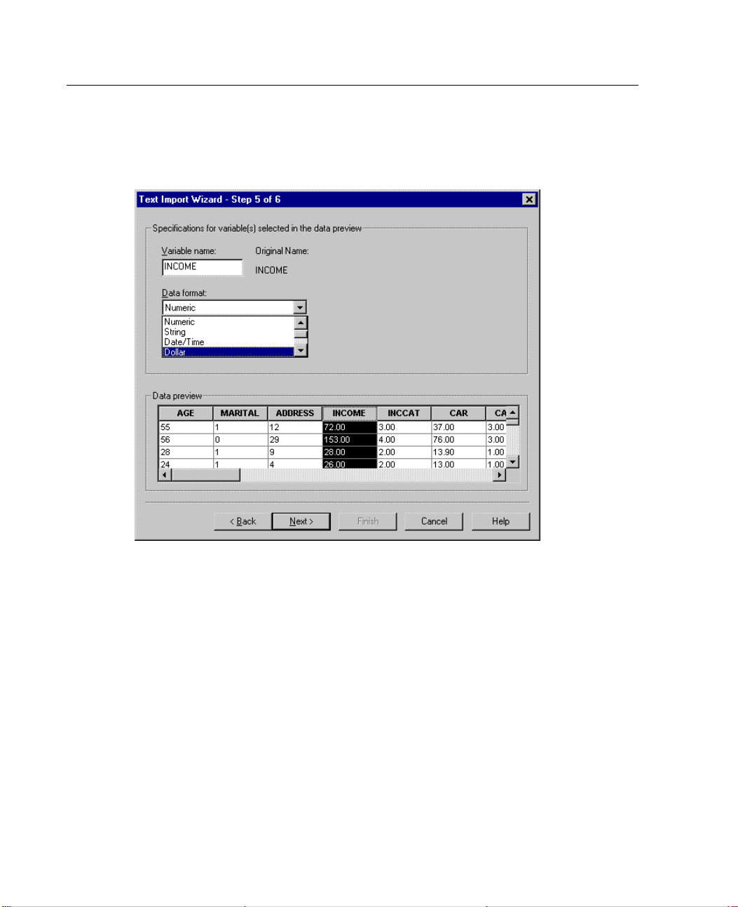
Data types can be defined here as well. For example, it’s safe to assume that the
income variable is meant to contain a certain dollar amount.
To change a data type:
E Under Data preview, select the variable you want to change, which is Income in
this case.
Page 62
48
Chapter 3
E
Select Dollar from the Data format drop-down list.
Figure 3-22
Change the da
E Click Next to continue.
ta type
Page 63
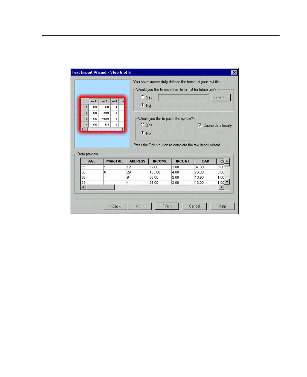
Figure 3-23
Text Import Wizard - Step 6 of 6
49
Reading Data
E Leave the default selections in this dialog box, and click Finish to import the data.
Saving Data
To save an SPSS data file, the Data Editor window must be the active window.
E From the menus choose:
File
Save
Browse to the desired directory.
E
Page 64

50
Chapter 3
E
TypeanameforthefileintheFilenametextbox.
The Variable
s button can be used to select which variables in the Data Editor are
saved to the SPSS data file. By default, all variables in the Data Editor are retained.
E Click Save.
The name in the title bar of the Data Editor will change to the filename you specified.
This confirms that the file has been successfully saved as an SPSS data file. The file
contains bo
th variable information (names, type, and, if provided, labels and missing
value codes), and all data values.
Page 65

Chapter
4
Using the Dat
The Data Editor displays the contents of the active data file. The information in the
Data Editor
In Data Vie
(observations).
In Variable View, each row is a variable, and each column is an attribute
associated with that variable.
Variables are used to represent the different types of data that you have compiled. A
common ana
equivalent to a variable. Variables come in many different types, including numbers,
strings, currency, and dates.
Entering Numeric Data
Data can be entered into the Data Editor, which may be useful for small data files or
for making minor edits to larger data files.
consists of variables and cases.
w, columns represent variables and rows represent cases
logy is that of a survey. The response to each question on a survey is
aEditor
E Click the Variable View tab at the bottom of the Data Editor window.
Define the
needed: age, marital status,andincome.
variables that are going to be used. In this case, only three variables are
51
Page 66
52
Chapter 4
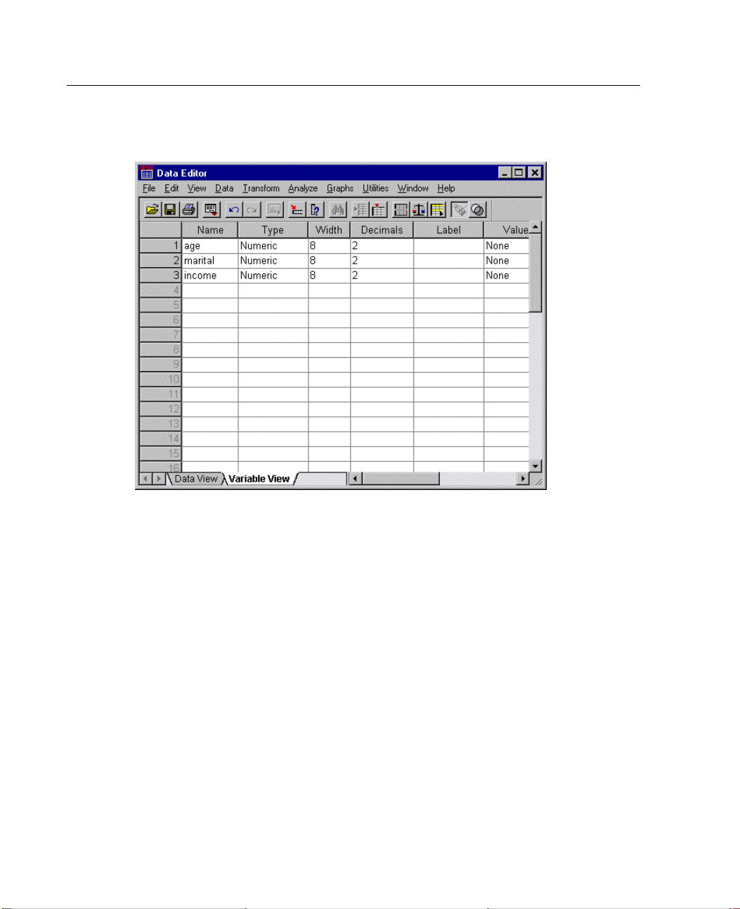
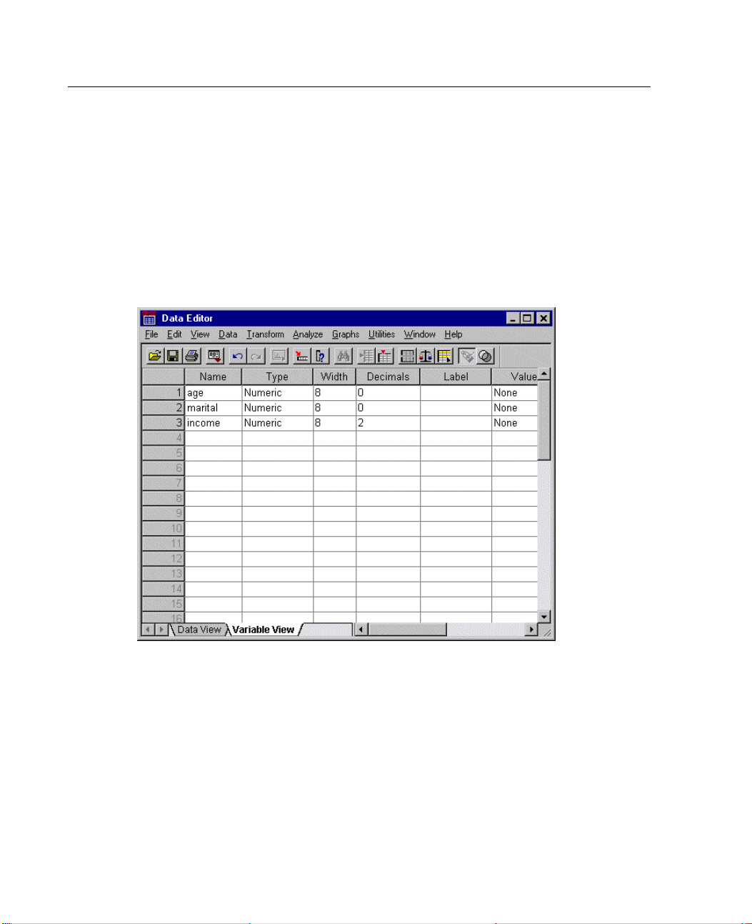
Figure 4-1
Variable names in Variable View
E In the first row of the first column, type age.
E In the second row, type marital.
E In the third row, type income.
New variables are automatically given a numeric data type.
If you do
n’t enter variable names, unique names are automatically created. However,
these names are not descriptive and are not recommended for large data files.
E Click the Data View tab to continue entering the data.
The names that you entered in Variable View are now the headings for the first three
columns i
nDataView.
Page 67
53
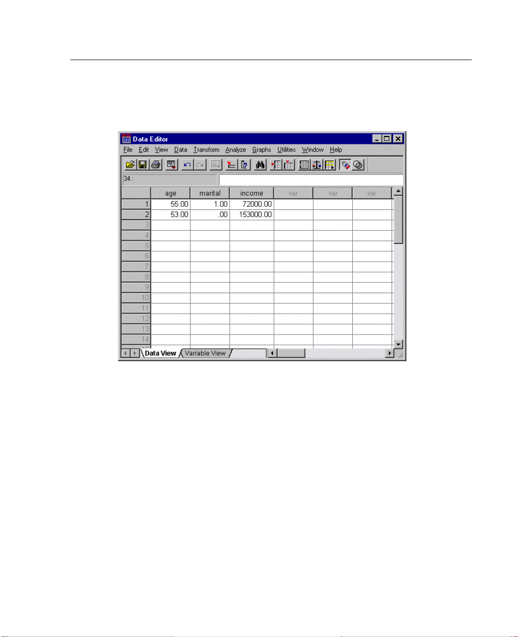
Begin entering data in the first row, starting at the first column.
Figure 4-2
Values enter
ed in Data View
Using the Data E
ditor
E In the a
E In the
E In the i
E Move th
E In the a
E In the m
E In the i
ge column, type
marital column, type
ncome column, type
55.
1.
72000.
e cursor to the first column of the second row to add the next subject’s data.
ge column, type
arital column, type
ncome column, type
53.
0.
153000.
Page 68
54
Chapter 4
Currently, the age and marital columns display decimal points, even though their
values are intended to be integers. To hide the decimal points in these variables:
E Click the Variable View tab at the bottom of the Data Editor window.
E Select the Decimals column in the age row and type 0 to hide the decimal.
E Select the Decimals column in the marital row and type 0 to hide the decimal.
Figure 4-3
Updated decimal property for age and marital
Enteri
ng String Data
Non-nu
E Click t
E In the f
meric data, such as strings of text, can also be entered into the Data Editor.
Variable View tab at the bottom of the Data Editor window.
he
irst cell of the first empty row, type
sex for the variable name.
Page 69
55
Using the Data E
E
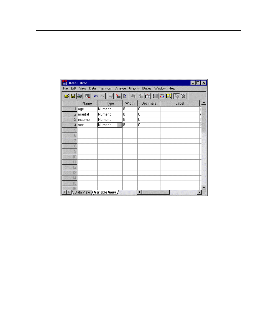
Click the Type cell.
E Click the button in the Type cell to open the Variable Type dialog box.
Figure 4-4
Button shown
in Type cell for sex
ditor
E Selec
String to specify the variable type.
t
Page 70
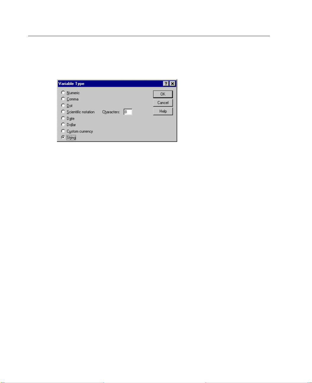
56
Chapter 4
E
Click OK to save your changes and return to the Data Editor.
Defining
Figure 4-5
Varia ble Typ
Data
In additi
e dialog box
on to defining data types, you can also define descriptive variable and value
labels for variable names and data values. These descriptive labels are used in
statistical reports and charts.
Adding a Variable Label
Labels are meant to provide descriptions of variables. These descriptions are often
longer versions of variable names. Labels can be up to 256 characters long. These
labels a
re used in your output to identify the different variables.
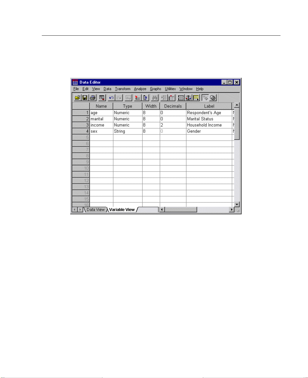
E Click t
E In the La
E In the La
E In the La
he
Variable View tab at the bottom of the Data Editor window.
bel column of the age row, type
bel column of the marital row, type
bel column of the income row, type
Respondent's Age.
Marital Status.
Household Income.
Page 71
57
E
In the Label column of the sex row, type Gender.
Figure 4-6
Varia ble lab
els entered in Variable View
Using the Data E
ditor
Changing Variable Type and Format
The Type column displays the current data type for each variable. The most common
are num
file, the income variable is defined as a numeric type.
E Click the Type cell for the income row, and then click the button to open the Variable
Type dialog box.
eric and string, but many other formats are supported. In the current data
Page 72
58
Chapter 4
E
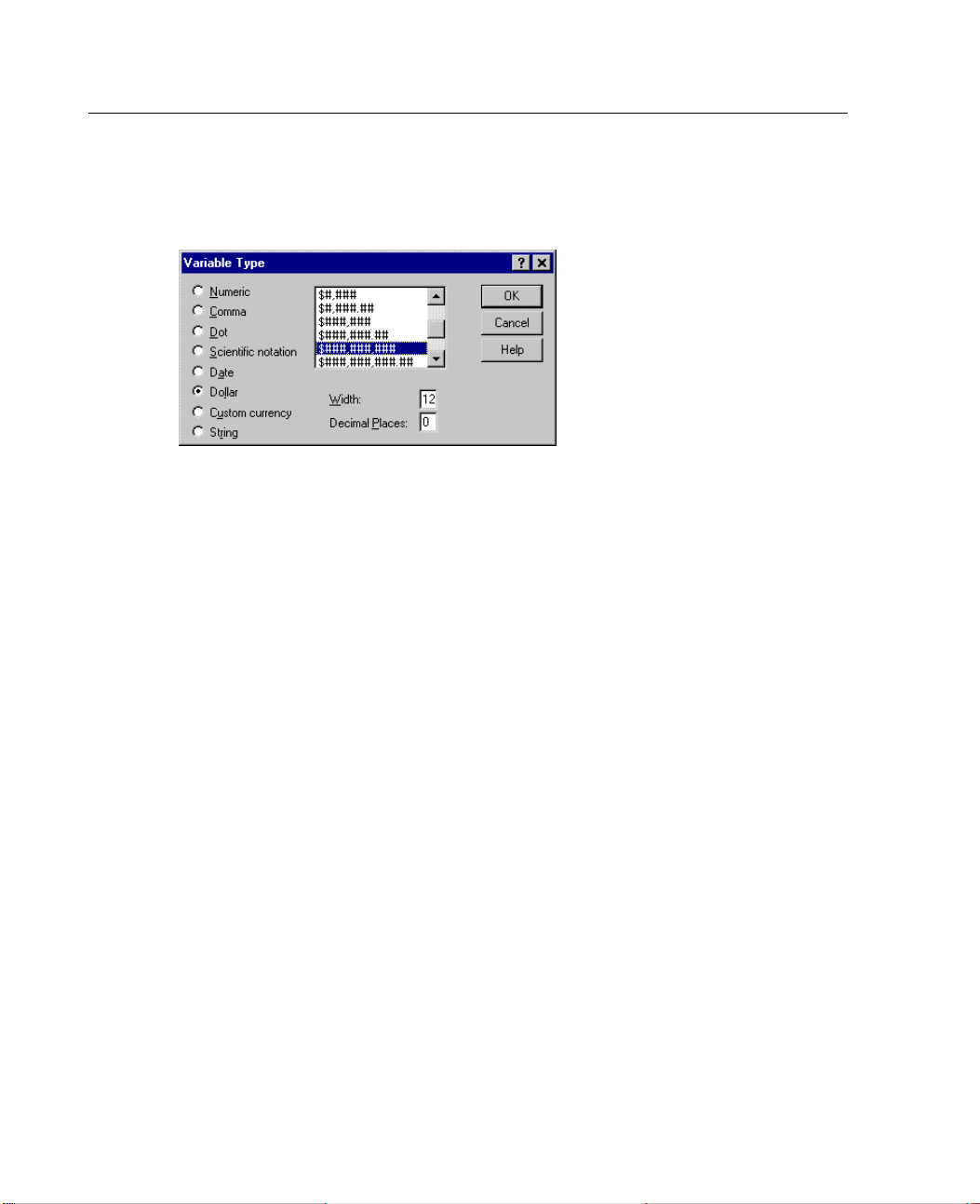
Select Dollar intheVariableTypedialogbox.
Figure 4-7
Varia ble Typ
The formatting options for the currently selected data type are displayed.
E Select the format of this currency. For this example, select $###,###,###.
E Click OK to save your changes.
Adding Val
Value labe
the case of this example, there are two acceptable values for the marital variable.
A value of 0 means that the subject is single, and a value of 1 means that he or
she is mar
e dialog box
ue Labels for Numeric Variables
ls provide a method for mapping your variable values to a string label. In
ried.
E Click th
e Values cell for the marital row, and then click the button to open the Value
Labels dialog box.
The value is the actual numeric value.
The value l
E Type 0 in t
E Type Sing
abel is the string label applied to the specified numeric value.
he Value field.
le
in the Value Label field.
Page 73
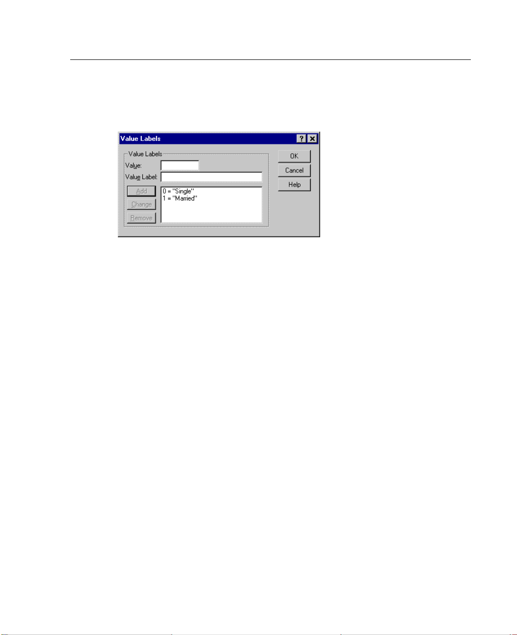
59
Using the Data E
E
Click Add to add this label to the list.
Figure 4-8
Value La bel s
E Repeat the process, this time typing 1 in the Value field and Married in the Value
dialog box
Label field.
E Click Add, and then click OK to save your changes and return to the Data Editor.
These labels can also be displayed in Data View, which can help to make your data
more readable.
E Click the Data View tab at the bottom of the Data Editor window.
ditor
E From the menus choose:
View
Value Labels
The labels are now displayed in a list when you enter values in the Data Editor. This
has the benefit of suggesting a valid response and providing a more descriptive answer.
Page 74
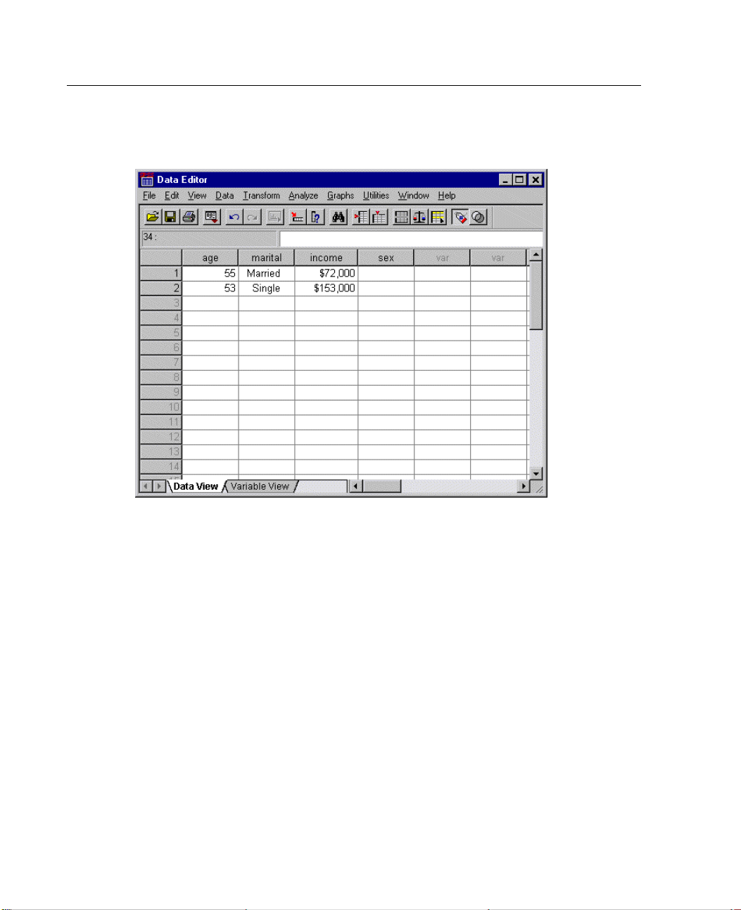
60
Chapter 4
Figure 4-9
Value labels displayed in Data View
Adding Value Labels for String Variables
String variables may require value labels as well. For example, your data may use
letters, M or F, to identify the sex of the subject. Value labels can be used to
single
specify that M stands for Male and F stands for Female.
E Click the Variable View tab at the bottom of the Data Editor window.
E Click the Values cell in the sex row,andthenclickthebuttontoopentheValue
Labels dialog box.
E Type F in the Value field, and then type Female in the Value Label field.
Page 75
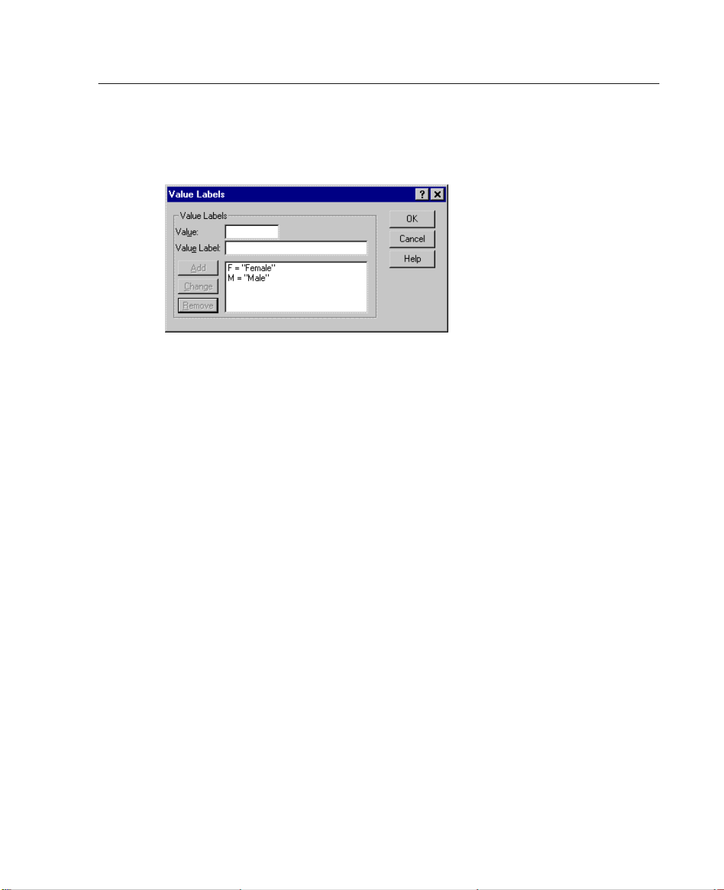
61
Using the Data E
E
Click Add to add this label to your data file.
Figure 4-10
Value La bel s
E Repeat the process, this time typing M in the Value field and Male in the Value
dialog box
Label field.
E Click Add, and then click OK to save your changes and return to the Data Editor.
Because string values are case sensitive, you should make sure that you are consistent.
Alowercasem is not the same as an uppercase M.
ditor
Using Value Labels for Data Entry
In a previous example, we chose to have value labels displayed rather than the
actual data by selecting Value Labels from the View menu. You can use these values
for data entry.
E Click the Data View tab at the bottom of the Data Editor window.
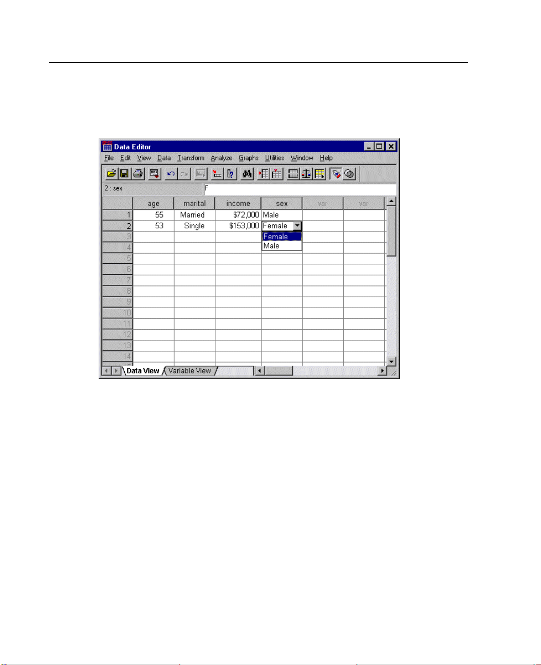
E In the first row, select the cell for sex and select Male from the drop-down list.
Page 76
62
Chapter 4
E
In the second row, select the cell for sex and select Female from the drop-down list.
Figure 4-11
Using variab
Only de
le labels to select values
fined values are listed, which helps to ensure that the data entered are in a
format that you expect.
Handli
ng Missing Data
g or invalid data are generally too common to ignore. Survey respondents may
Missin
refuse to answer certain questions, may not know the answer, or may answer in
an unexpected format. If you don’t take steps to filter or identify these data, your
sis may not provide accurate results.
analy
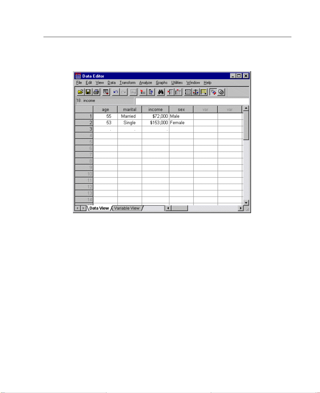
For numeric data, empty data fields or fields containing invalid entries are handled
by converting the fields to system missing, which is identifiable by a single period.
Page 77
63
Figure 4-12
Missing values displayed as periods
Using the Data E
ditor
Missin
The reason a value is missing may be important to your analysis. For example, you
may fin
ditusefultodistinguishbetweenthosewhorefusedtoansweraquestionand
those who didn’t answer a question because it was not applicable.
g Values for a Numeric Variable
Variable View tab at the bottom of the Data Editor window.
E Click
E Click
the
the Missing cell in the age row,andthenclickthebuttontoopentheMissing
Values dialog box.
Page 78
64
Chapter 4
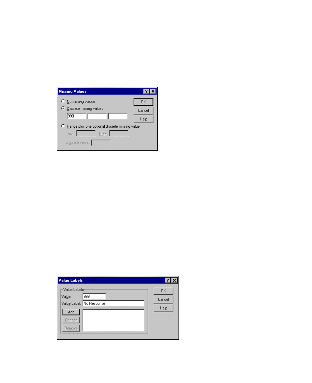
In this dialog box, you can specify up to three distinct missing values, or a range of
values plus one additional discrete value.
Figure 4-13
Missing Values dialog box
E Select Discrete missing values.
E Type 999 in the first text box and leave the other two empty.
E Click OK to save your changes and return to the Data Editor.
Now that the missing data value has been added, a label can be applied to that value.
E Click the Values cell in the age row,andthenclickthebuttontoopentheValue
Labels dialog box.
E Type 999 in the Value field.
E Type No Response in the Value Label field.
Figure 4-14
Value Labels dialog box
Page 79

65
E
Click Add to add this label to your data file.
E Click OK to save your changes and return to the Data Editor.
Missing Valu
Missing val
Unlike numeric values, empty fields in string variables are not designated as system
missing. Rather, they are interpreted as an empty string.
E Click the Variable View tab at the bottom of the Data Editor window.
E Click the Missing cell in the sex row,andthenclickthebuttontoopentheMissing
Values dial
E Select Dis
E Type NR in t
Missing values for string variables are case sensitive. So, a value of nr is not treated
as a missing value.
Using the Data E
es for a String Variable
ues for string variables are handled similarly to those for numeric values.
og box.
crete missing values
hefirsttextbox.
.
ditor
E Click OK to save your changes and return to the Data Editor.
Now you can add a label for the missing value.
E Click the Values cell in the sex row,andthenclickthebuttontoopentheValue
Labels dialo
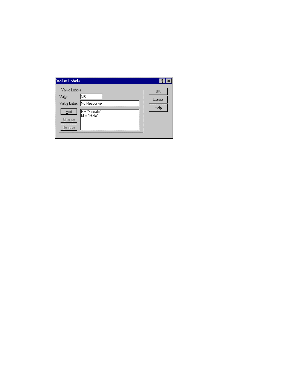
E Type NR in th
gbox.
e Value field.
Page 80
66
Chapter 4
E
Type No Response in the Value Label field.
Figure 4-15
Value La bel s
E Click Add to add this label to your project.
E Click OK to save your changes and return to the Data Editor.
dialog box
Copying and Pasting Value Attributes
Once you’ve defined variable attributes for a variable, you can copy these attributes
and apply them to other variables.
Page 81
67
E
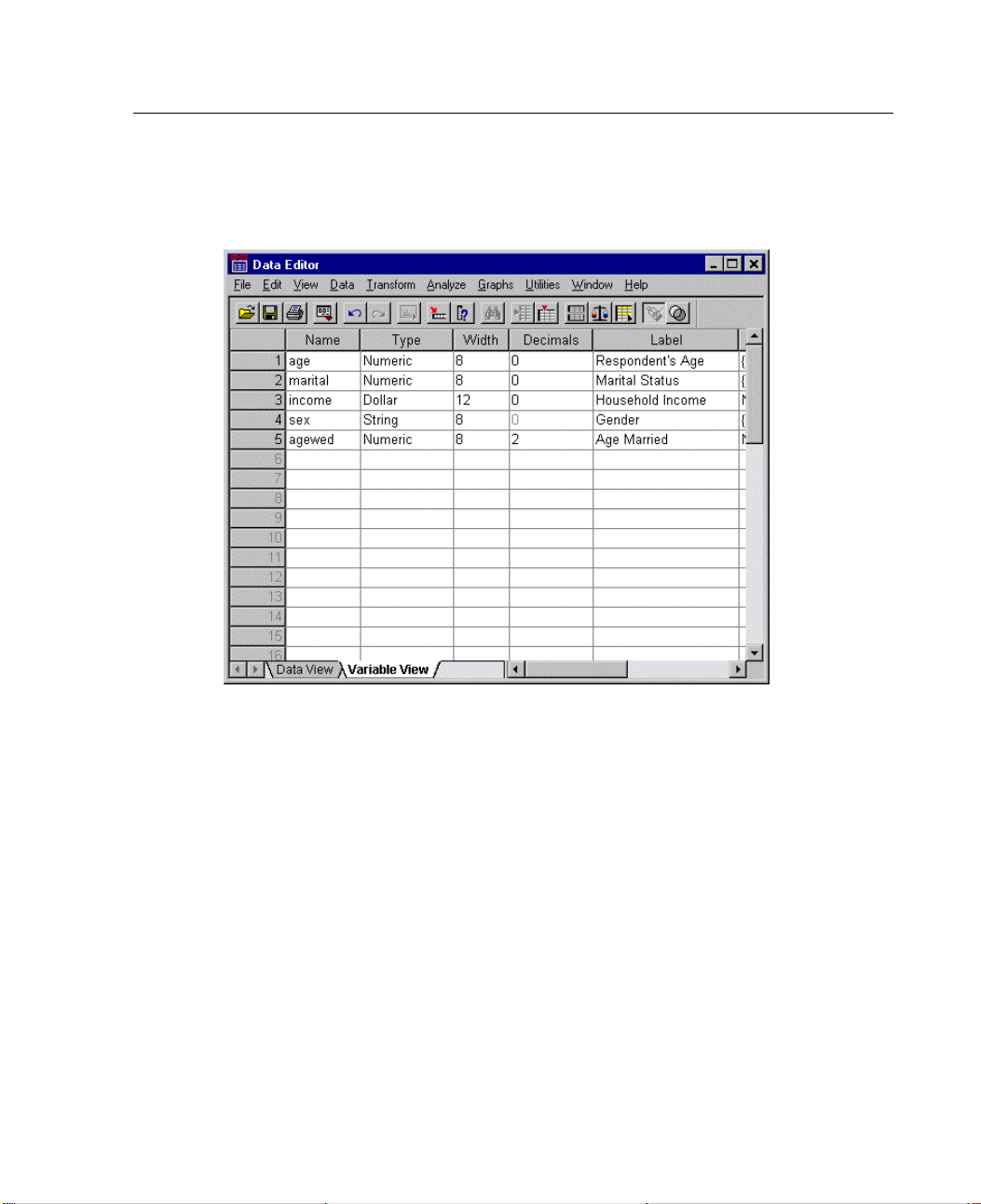
In Variable View, type agewed in the first cell of the first empty row.
Figure 4-16
agewed varia
bleinVariableView
Using the Data E
ditor
E In the
E Click t
E From th
E
E From the menus choose:
Label column, type
he Values cell in the age row.
e menus choose:
Edit
Copy
Click the Values cell in the agewed row.
Edit
Paste
Age Married.
Page 82
68
Chapter 4
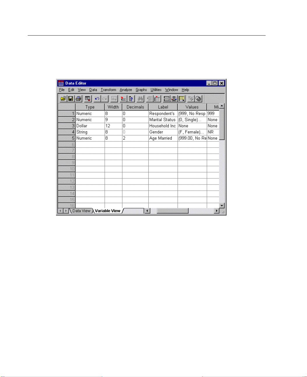
The defined values from the age variable are now applied to the agewed variable.
Figure 4-17
Values paste
dforagewed
Page 83
69
Using the Data E
ditor
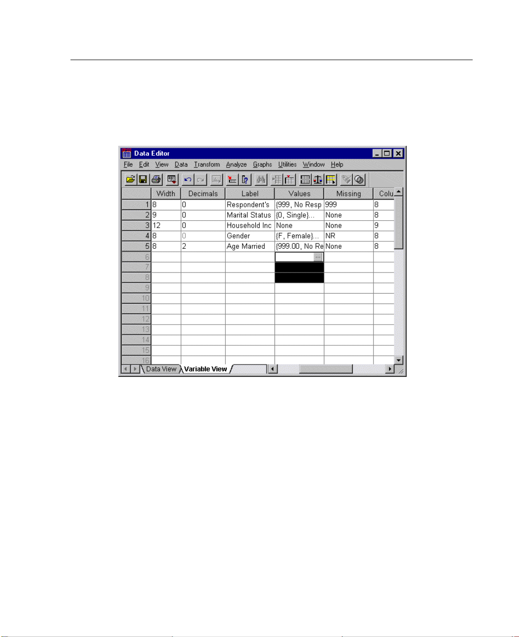
To apply the attribute to multiple variables, simply select multiple target cells (click
anddragdownthecolumn).
Figure 4-18
Multiple cells selected
Page 84
70
Chapter 4
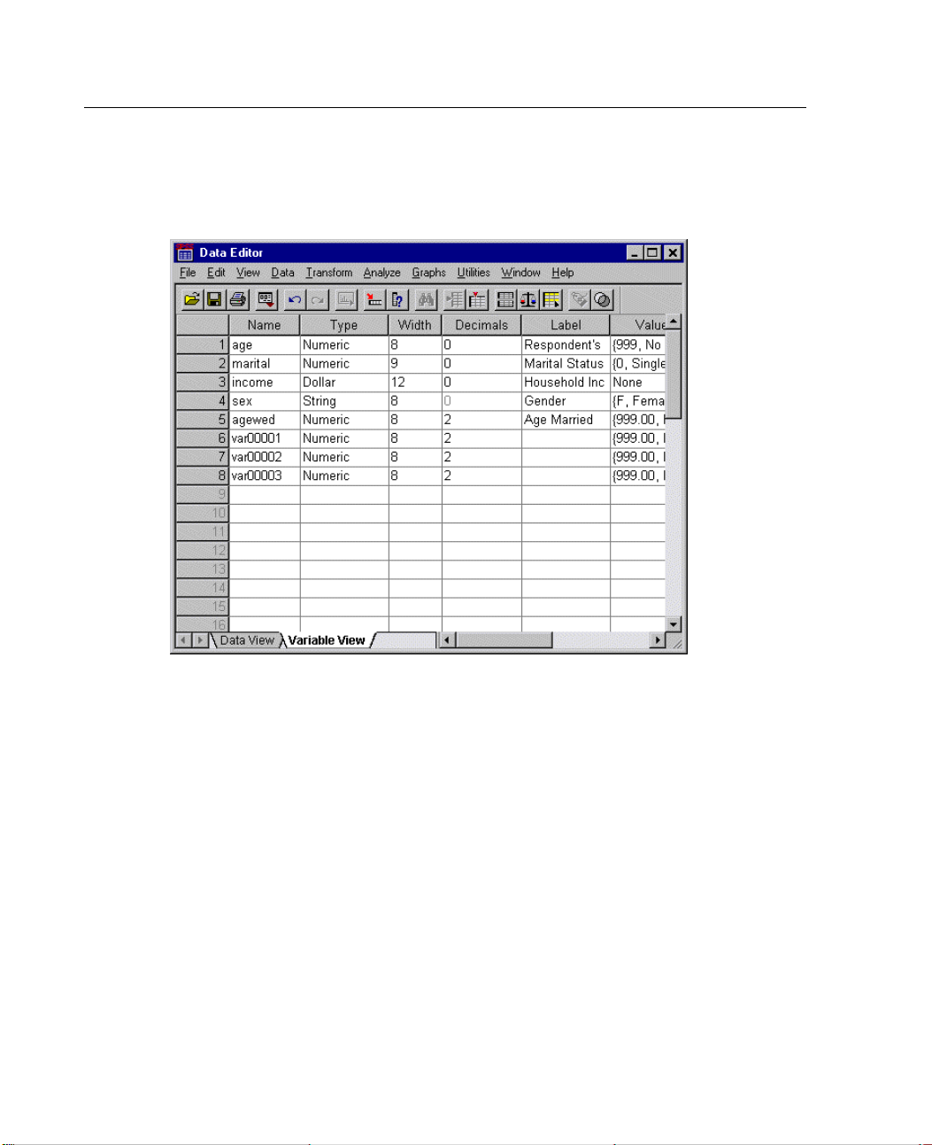
When you paste the attribute, it is applied to all of the selected cells.
Figure 4-19
Values paste
dintomultiplecells
New variables are automatically created if you paste the values into empty rows.
You can also copy all of the attributes from one variable to another.
Page 85
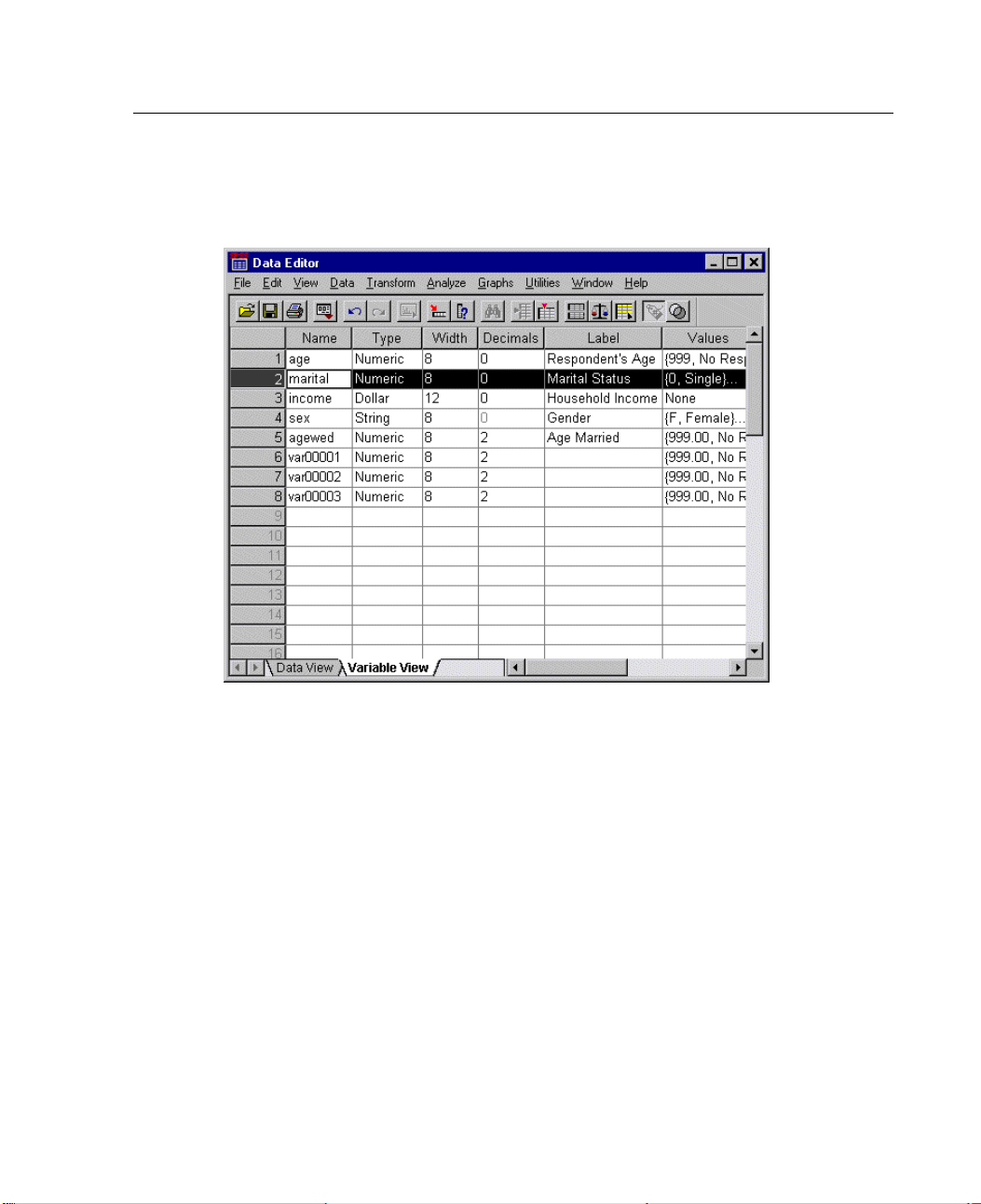
71
E
Click the row number in the marital row.
Figure 4-20
Selected row
Using the Data E
ditor
E From th
Edit
E
Click the row number of the first empty row.
E From the menus choose:
Edit
e menus choose:
Copy
Paste
Page 86
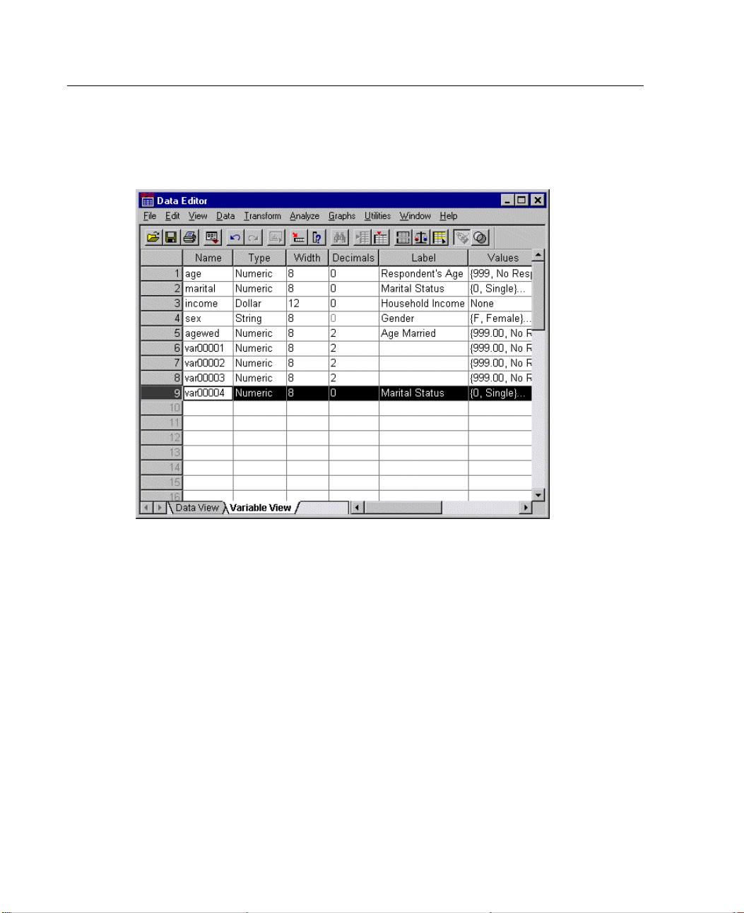
72
Chapter 4
All of the attributes of the marital variable are applied to the new variable.
Figure 4-21
Values paste
dintorow
Defining Variable Properties for Categorical Variables
For categorical (nominal, ordinal) data, Define Variable Properties can help you
value labels and other variable properties. Define Variable Properties:
define
Scans
Identifies unlabeled values and provides an “auto-label” feature.
Provides the ability to copy defined value labels from another variable to the
the actual data values and lists all unique data values for each selected
variable.
selected variable or from the selected variable to multiple additional variables.
Page 87
73
Using the Data E
ditor
This example uses the data file demo.sav. This data file already has defined value
labels; so before we start, let’s enter a value for which there is no defined value label:
E InDataViewoftheDataEditor,clickthefirstdatacellforthevariableownpc (you
may have to sc
E From the men
Data
Define Variable Properties...
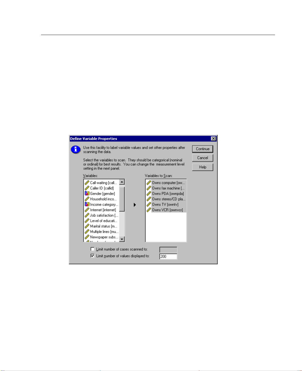
Figure 4-22
Initial Defi
roll to the right) and enter the value
us choose:
ne Variable Properties dialog box
99.
In the initial Define Variable Properties dialog box, you select the nominal or ordinal
variables for which you want to define value labels and/or other properties.
Since Define Variable Properties relies on actual values in the data file to help you
make good choices, it needs to read the data file first. This can take some time if your
data file contains a very large number of cases, so this dialog box also allows you
to limit the number of cases to read, or scan. Limiting the number of cases is not
Page 88
74
Chapter 4
necessary for our sample data file. Even though it contains over 6,000 cases, it
doesn’t take very long to scan that many cases.
E Drag and drop Owns computer [ownpc] through Owns VCR [ownvcr] into the
Variables t
oScanlist.
You might notice that the measurement level icons for all of the selected variables
indicate that they are scale variables, not categorical variables. By default, all numeric
variables a
re assigned the scale measurement level, even if the numeric values are
actually just codes that represent categories. All of the selected variables in this
example are really categorical variables that use the numeric values 0 and 1 to stand
for No and Y
es, respectively—and one of the variable properties that we’ll change
with Define Variable Properties is the measurement level.
E Click Continue.
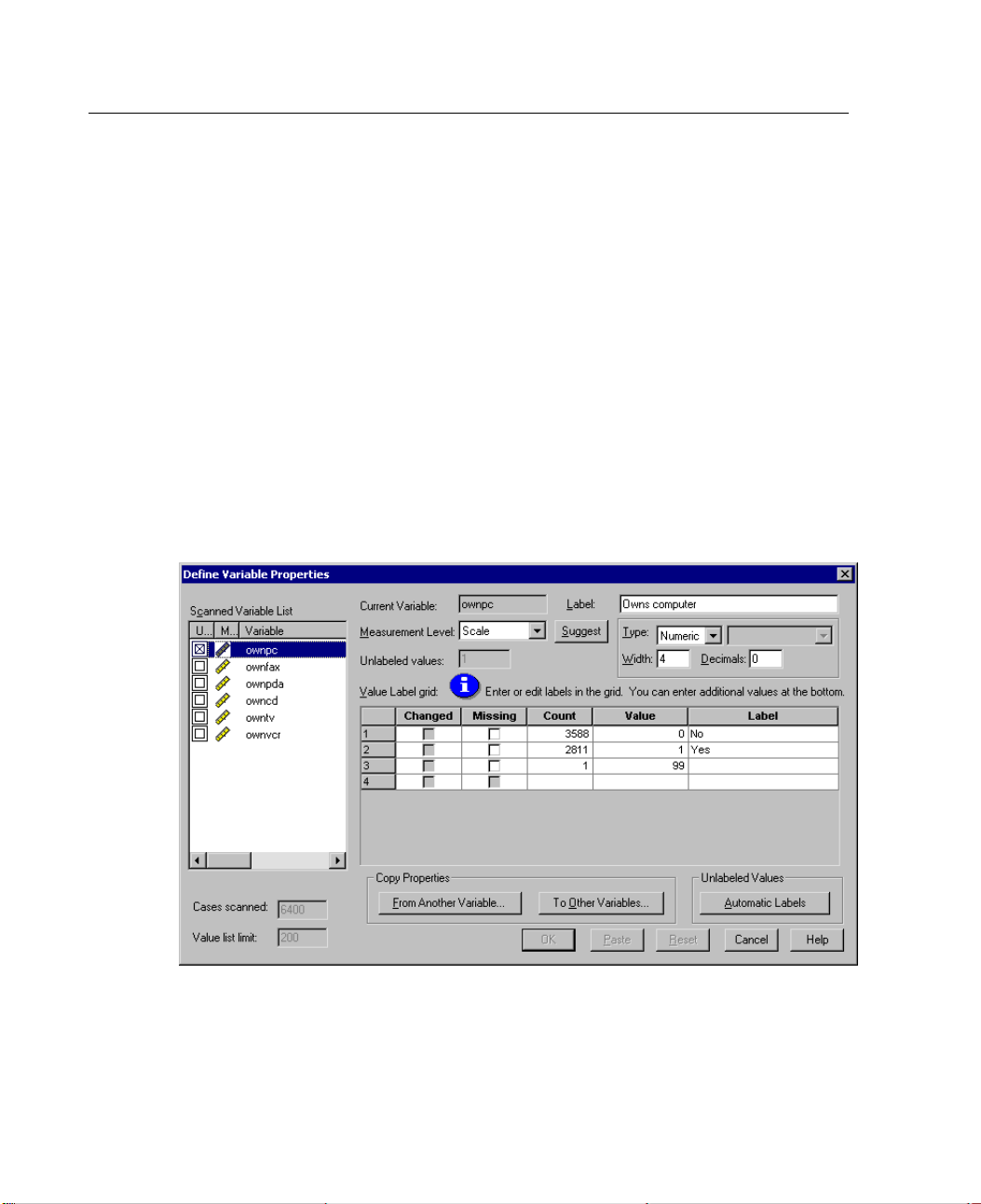
Figure 4-2
Define Var
E In the Scanned Variable List, select ownpc.
3
iable Properties main dialog box
Page 89
75
Using the Data E
The current level of measurement for the selected variable is scale. You can change
the measurement level by selecting one from the drop-down list or you can let Define
Variable Pr
E Click Sugge
Figure 4-24
Suggest Measurement Level dialog box
operties suggest a measurement level.
.
st
ditor
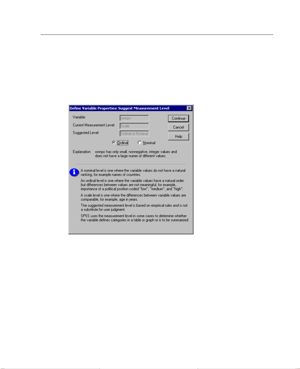
Since the variable doesn’t havevery many different values and all of the scanned cases
n integer values, the proper measurement level is probably ordinal or nominal.
contai
E Select
Ordinal and then click Continue.
The measurement level for the selected variable is now ordinal.
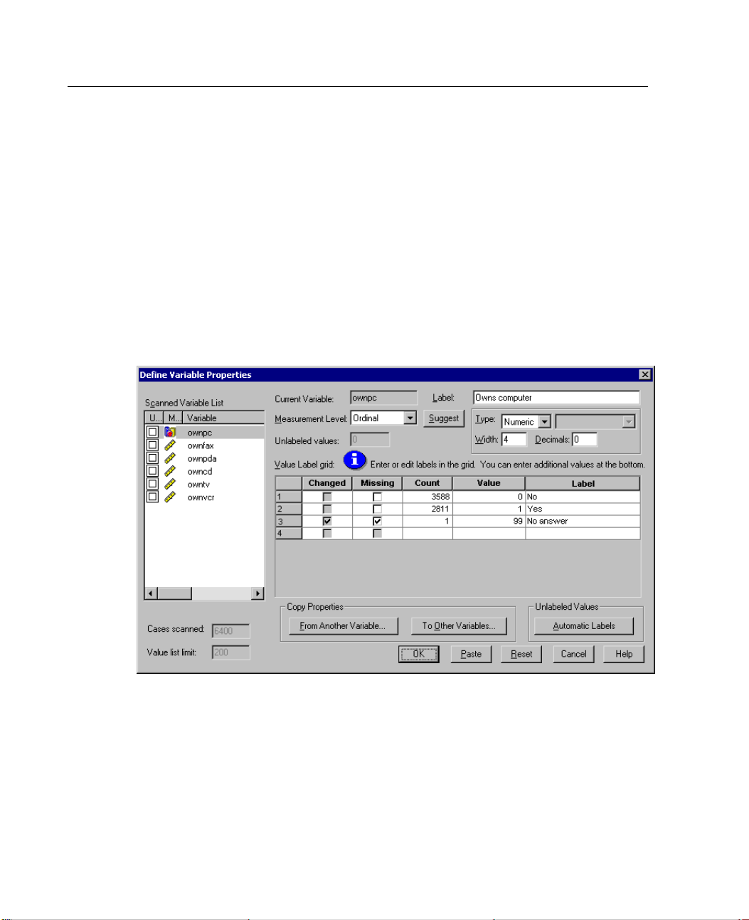
The Value Labels Grid displays all of the unique data values for the selected variable,
any defi
ned value labels for these values, and the number of times (count) each
value occurs in the scanned cases.
Page 90
76
Chapter 4
The value that we entered, 99, is displayed in the grid. The count is only 1 because
we changed the value for only one case, and the Label column is empty because we
haven’t def
ined a value label for 99 yet. An
X in the first column of the Scanned
Variable List also indicates that the selected variable has at least one observed value
without a defined value label.
E In the Label columnforthevalueof99,enterNo answer.
E Then click (check) the box in the Missing column. This identifies the value 99 as user
missing.Da
ta values specified as user missing are flagged for special treatment and
are excluded from most calculations.
Figure 4-25
New variabl
e properties defined for ownpc
Before we complete the job of modifying the variable properties for ownpc,let’s
he same measurement level, value labels, and missing values definitions to
apply t
the other variables in the list.
E In the Copy Properties group, click To Other Variables.
Page 91
77
Figure 4-26
Apply Labels and Level dialog box
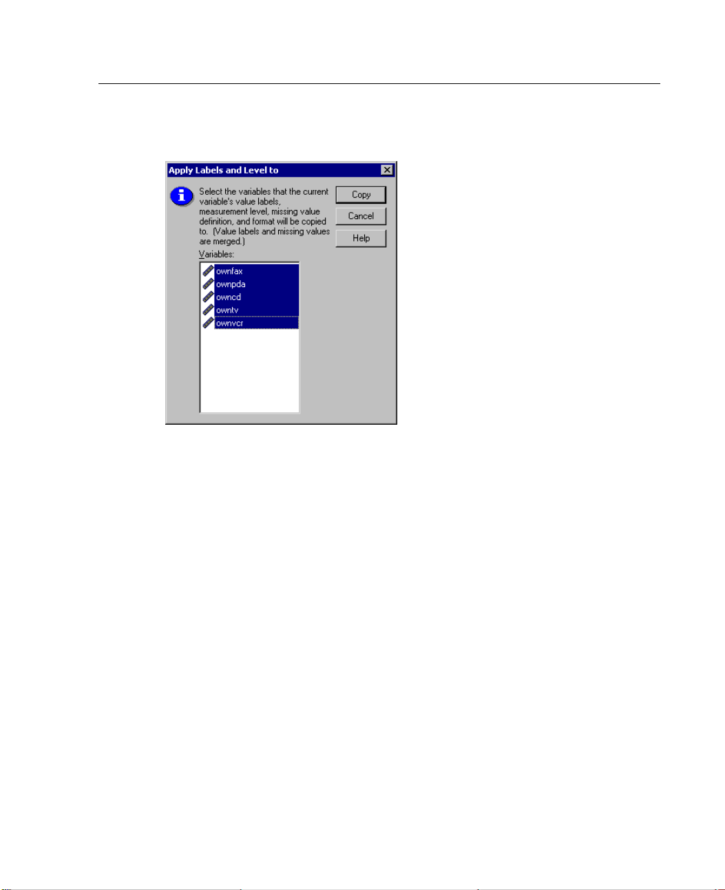
In the Ap
then click
ply Labels and Level dialog box, select all of the variables in the list, and
Copy.
Using the Data E
ditor
Page 92
78
Chapter 4
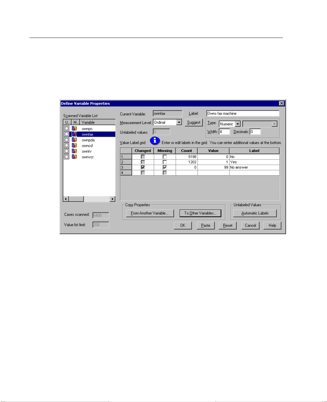
If you select any other variable in the list in the Define Variable Properties main
dialog box now, you’ll see that they are all now ordinal variables, with a value of 99
defined as u
Figure 4-27
New variable properties defined for ownfax
ser missing and a value label of No answer.
E Click OK to save all of the variable properties that you have defined.
Page 93

Chapter
5
Examining S u
mmary Statistics
for Individual Variables
This chapt
of a variable influences the types of statistics that should be used. We will use the
data file demo.sav.
Level of Measurement
Different summary measures are appropriate for different types of data, depending
on the level of measurement:
Categoric
gender or marital status). Also referred to as qualitative data. Categorical variables
can be string (alphanumeric) data or numeric variables that use numeric codes to
represen
basic types of categorical data:
Nominal. Categorical data where there is no inherent order to the categories. For
Ordinal. Categorical data where there is a meaningful order of categories, but
er discusses simple summary measures and how the level of measurement
al.
Data with a limited number of distinct values or categories (for example,
t categories (for example, 0 = U nmarried and 1 = Married). There are two
example,
“marketing” or “research.”
there isn’t a measurable distance between categories. For example, there is
an order t
values can’t be calculated.
a job category of “sales” isn’t higher or lower than a job category of
o the values high, medium, and low, but the “distance” between the
79
Page 94
80
Chapter 5
Scale. Data measured on an interval or ratio scale, where the data values indicate
both the order of values and the distance between values. For example, a salary of
$72,195 is h
igher than a salary of $52,398, and the distance between the two values is
$19,797. Also referred to as quantitative or continuous data.
Summary Mea
For categor
of cases in each category. The mode is the category with the greatest number of cases.
For ordinal data, the median (the value above and below which half the cases fall)
mayalsobe
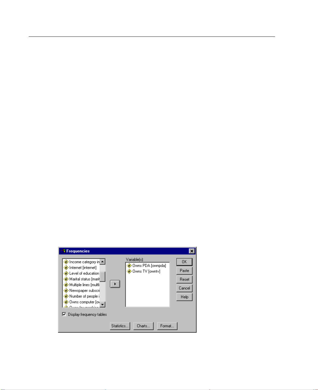
The Frequencies procedure produces frequency tables that display both the number
and percentage of cases for each observed value of a variable.
E From the menus choose:
Analyze
Descripti
Frequenci
Select Ow
E
list.
Figure 5-1
Categoric
sures f or Categorical Data
ical data, the most typical summary measure is the number or percentage
a useful summary measure if there is a large number of categories.
ve Statistics
es...
ns PDA (ownpda) and Owns TV (owntv) and move them into the Variable(s)
al variables selected for analysis
E Click OK to run the procedure.
Page 95
81
Figure 5-2
Frequency tables
Examining Summ
ary Statistics for Individual Variables
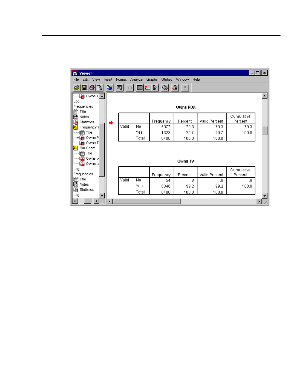
The frequency tables are displayed in theViewerwindow.Thefrequencytables
reveal that only about 21% of the people own PDAs, but almost everybody owns a TV
(99.2%). This might not be an interesting revelation, although it might be interesting
to find out more about the small group of people who do not own televisions.
Charts for Categorical Data
You can graphically display the information in a frequency table with a bar chart
or pie chart.
E Open the Frequencies dialog box again. (The two variables should still be selected.)
Page 96
82
Chapter 5
You can use the Dialog Recall button on the toolbar to quickly return to recently
used procedures.
Figure 5-3
Dialog Recall tool
.
E Click Char
E Select Bar
Figure 5-4
Frequencies Charts dialog box
ts
andthenclickContinue.
charts
E Click OK in the main dialog box to run the procedure.
Page 97
83
Figure 5-5
Bar chart
Examining Summ
ary Statistics for Individual Variables
Summar
E Open
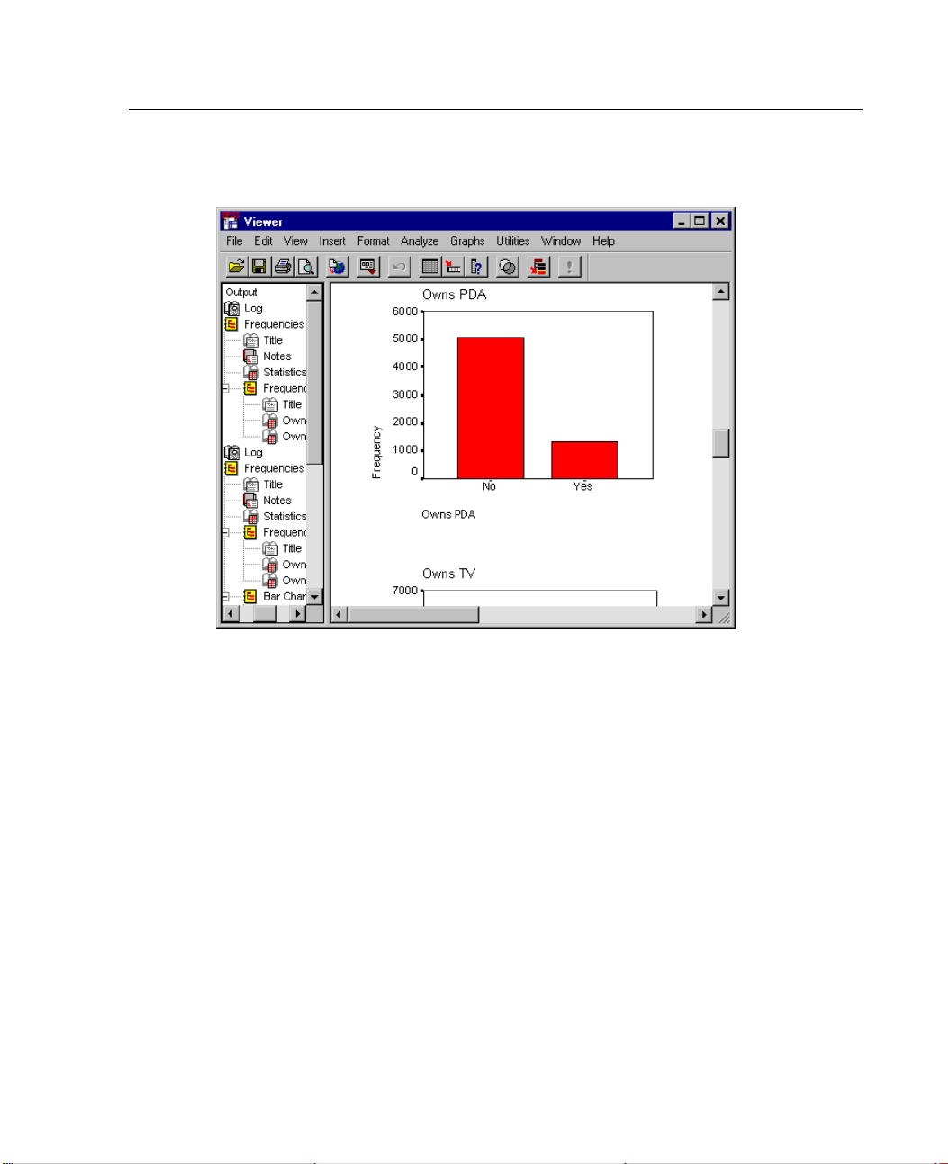
In addition to the frequency tables, the same information is now displayed in the form
of bar c
harts, making it easy to see that most people do not own PDAs but almost
everyone owns a TV.
y Measures for Scale Variables
are many summary measures available for scale variables, including:
There
Meas
ures of central tendency.
are the mean (arithmetic average) and median (value above and below which
half the cases fall).
Measures of dispersion. Statistics that measure the amount of variation or spread
data include the standard deviation, minimum, and maximum.
in the
the Frequencies dialog box again.
The most common measures of central tendency
Page 98
84
Chapter 5
E
Click Reset to clear any previous settings.
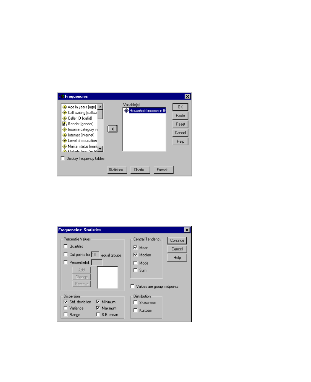
E Select Household income in thousands (income) and move it into the Variable(s) list.
Figure 5-6
Scale variab
E Click Statistics.
E Select Mean, Median, Std. deviation, Minimum,andMaximum.
Figure 5-7
Frequencies Statistics dialog box
le selected for analysis
E Click Continue.
Page 99
85
Examining Summ
E
Deselect Displayfrequency tablesin the main dialog box. (Frequency tables are usually
ary Statistics for Individual Variables
not useful for scale variables since there may be almost as many distinct values as
there are ca
E Click OK to
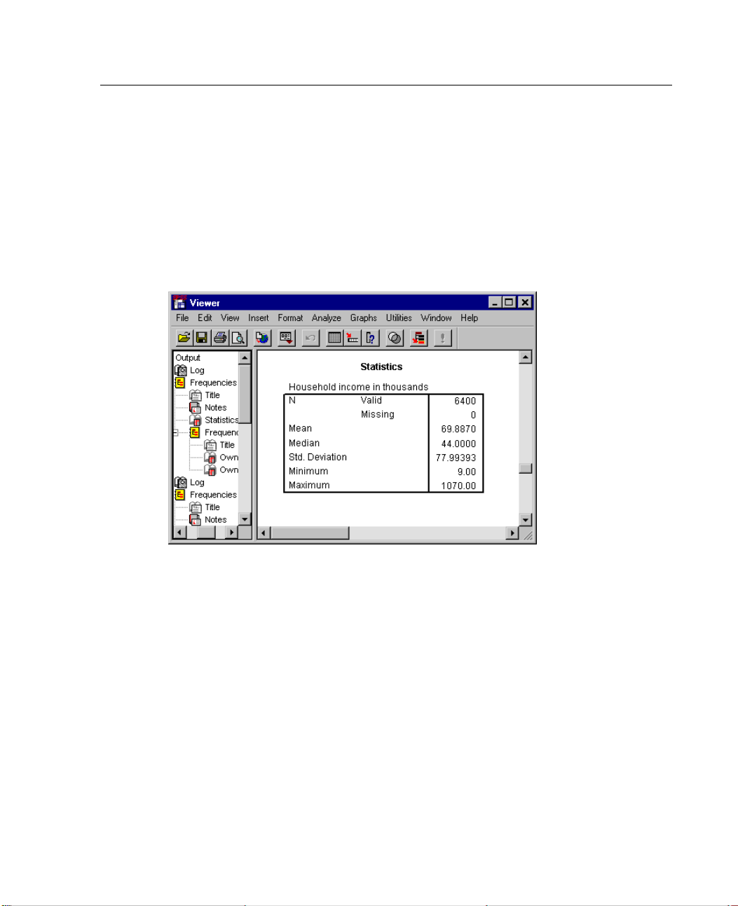
The Frequenc
Figure 5-8
Frequencies Statistics table
ses in the data file.)
run the procedure.
ies Statistics table is displayed in the Viewer window.
In this example, there is a large difference between the mean and the median, with the
mean bei
ng more than 25,000 greater than the median. This indicates that the values
are not normally distributed. We can visually check the distribution with a histogram.
Page 100
86
Chapter 5
Histograms for Scale Variables
E Open the Frequencies dialog box again.
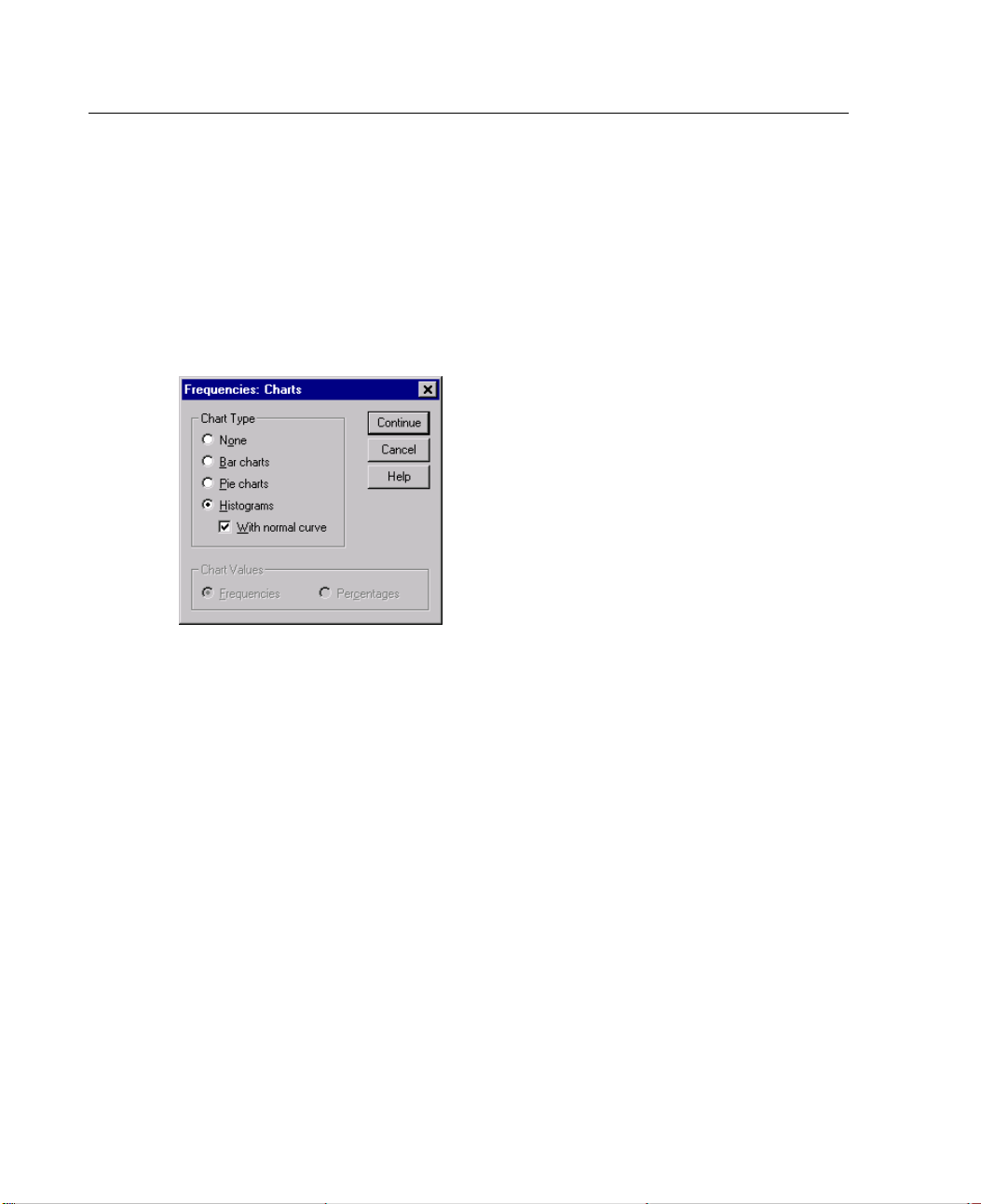
E Click Charts.
E Select Histograms and With normal curve.
Figure 5-9
Frequencies
E Click Continue and click OK in the main dialog box to run the procedure.
Charts dialog box
 Loading...