Siemens 6AU1900-1AB32-0BA0 User Manual

Download

SIMOTION CamTool

Configuration Manual

Preface

Description

Installing the Software

Configuring

Functions

12.2004 6AU1900-1AB32-0BA0

Safety Guidelines

This manual contains notices you have to observe in order to ensure your personal safety, as well as to prevent damage to property. The notices referring to your personal safety are highlighted in the manual by a safety alert symbol, notices referring to property damage only have no safety alert symbol. These notices shown below are graded according to the degree of danger.

Danger

indicates that death or severe personal injury will result if proper precautions are not taken.

Warning

indicates that death or severe personal injury may result if proper precautions are not taken.

Caution

with a safety alert symbol, indicates that minor personal injury can result if proper precautions are not taken.

Caution

without a safety alert symbol, indicates that property damage can result if proper precautions are not taken.

Attention

indicates that an unintended result or situation can occur if the corresponding information is not taken into account.

If more than one degree of danger is present, the warning notice representing the highest degree of danger will be used. A notice warning of injury to persons with a safety alert symbol may also include a warning relating to property damage.

Qualified Personnel

The device/system may only be set up and used in conjunction with this documentation. Commissioning and operation of a device/system may only be performed by qualified personnel. Within the context of the safety notes in this documentation qualified persons are defined as persons who are authorized to commission, ground and label devices, systems and circuits in accordance with established safety practices and standards.

Prescribed Usage

Note the following:

Warning

This device may only be used for the applications described in the catalog or the technical description and only in connection with devices or components from other manufacturers which have been approved or recommended by Siemens. Correct, reliable operation of the product requires proper transport, storage, positioning and assembly as well as careful operation and maintenance.

Trademarks

All names identified by ® are registered trademarks of the Siemens AG. The remaining trademarks in this publication may be trademarks whose use by third parties for their own purposes could violate the rights of the owner.

Copyright Siemens AG 2004. All rights reserved. The distribution and duplication of this document or the utiliz ation and transmission of its contents are not permitted without express written permission. Offenders will be liable for damages. All rights, including rights created by patent grant or registration of a utility model or design, are reserved.

Siemens AG Automation and Drives Postfach 4848, 90327 Nuremberg, Germany

Siemens Aktiengesellschaft 6AU1900-1AB32-0BA0

Disclaimer of Liability We have reviewed the contents of this publication to ensure consistency with the hardware and software described. Since variance cannot be precluded entirely, we cannot guarantee full consistency. However, the information in this publication is reviewed regularly and any necessary corrections are included in subsequent editions.

Siemens AG 2004 Technical data subject to change

Preface

Contents of manual

The accompanying manual describes the SIMOTION CamTool option package.

The document is part of the SIMOTION Engineering System documentation package with order number: 6AU1900-1AB32-0BA0, Edition 12.2004

Scope

The accompanying manual applies to SIMOTION SCOUT in conjunction with the SIMOTION CamTool option package.

Standards

The SIMOTION system was developed in accordance with the ISO 9001 quality guidelines.

Information blocks:

The following is a description of the purpose and use of the product manual.

• Description chapter

• Installation chapter

• Configuration chapter

• Functions chapter

This chapter provides a short overview of the basic functions of the SIMOTION CamTool and the inclusion in SIMOTION SCOUT.

This chapter describes how the SIMOTION CamTool is installed and which prerequisites must be satisfied to allow the use of SIMOTION CamTool.

This chapter describes the basic functions of SIMOTION CamTool. It shows you how to process cams with CamTool.

In this chapter you learn how to create a cam with CamTool.

CamTool Configuration Manual, 12.2004, 6AU1900-1AB32-0BA0

iii

Preface

SIMOTION documentation

An overview of the SIMOTION documentation is provided in a separate list of references.

The list of references is supplied on the "SIMOTION SCOUT" CD and is included in each print copy order of the documentation package.

The list of references can be obtained separately under the following MLFB number:

Order no.: 6AU1900-1AA32-0BA0

Edition 12.2004

SIMOTION documentation consists of 10 documentation packages containing approximately 50 SIMOTION documents and documents on other products (e.g., SINAMICS).

The following documentation packages are available for SIMOTION V3.2:

• SIMOTION Engineering System

• SIMOTION System and Function Descriptions

• SIMOTION Diagnostics

• SIMOTION Programming

• SIMOTION Programming - Reference Lists

Hotline

• SIMOTION C230

• SIMOTION P350

• SIMOTION D4xx (incl. SINAMICS S120)

• SIMOTION Supplementary Documentation

• SIMOTION Function Library

If you have any questions, please contact our hotline (worldwide):

• A & D Technical Support: Phone: +49 (180) 50 50 222

• Fax: +49 (180) 50 50 223

• E-mail: ad.support@siemens.com

If you have any questions, suggestions, or corrections regarding the documentation, please fax or e-mail them to the following:

• Fax: +49 (9131) 98 2176

• E-mail: motioncontrol.docu@erlf.siemens.de

• Fax form: refer to the reply form at the end of the document

CamTool

iv Configuration Manual, 12.2004, 6AU1900-1AB32-0BA0

Preface

Additional support

We also offer introductory courses to help you familiarize yourself with SIMOTION.

Please contact your regional training center or our main training center at D-90027 Nuremberg/Germany, phone +49 (911) 895 3202.

Siemens Internet address

The latest information on SIMOTION products can be found on the Internet at:

General information http://www.siemens.com/simotion

Technical information http://www4.ad.siemens.de/view/cs/de/10805438

CamTool Configuration Manual, 12.2004, 6AU1900-1AB32-0BA0

Preface ...................................................................................................................................................... iii

1 Description.............................................................................................................................................. 1-1

2 Installing the Software ............................................................................................................................ 2-1

2.1 Installing SIMOTION CamTool .................................................................................................. 2-1

2.2 Deinstalling SIMOTION CamTool ..............................................................................................2-2

3 Configuring ............................................................................................................................................. 3-1

3.1 Content....................................................................................................................................... 3-1

3.2 Customizing the Working Area Display ..................................................................................... 3-2

3.2.1 Changing the representation using the toolbar.......................................................................... 3-2

3.2.2 Maximizing working area ........................................................................................................... 3-4

3.3 Editing a Cam with CamTool ..................................................................................................... 3-5

3.3.1 Content....................................................................................................................................... 3-5

3.3.2 Adding a cam to a SCOUT project using CamTool ................................................................... 3-5

3.3.3 Edit cam created with CamEdit with CamTool........................................................................... 3-7

3.3.4 Import cam from text file .......................................................................................................... 3-10

3.3.5 Upload cam from SIMOTION device ....................................................................................... 3-12

3.4 Save cam ................................................................................................................................. 3-15

3.5 Customize the display of the cam ............................................................................................ 3-16

3.5.1 Display the cam ....................................................................................................................... 3-16

3.5.2 Show/hide diagram .................................................................................................................. 3-16

3.5.3 Change axis representation parameters.................................................................................. 3-17

3.5.4 Change diagram representation parameters ........................................................................... 3-20

3.5.5 Change lines and fonts representation parameters................................................................. 3-22

3.5.6 Displaying auxiliary lines in the diagram.................................................................................. 3-24

3.6 Download cam to SIMOTION device ....................................................................................... 3-26

4 Functions................................................................................................................................................ 4-1

4.1 Content....................................................................................................................................... 4-1

4.2 Structure of a cam...................................................................................................................... 4-2

4.3 Fixed point.................................................................................................................................. 4-3

4.3.1 Fixed Point Definition ................................................................................................................. 4-3

4.3.2 Insert fixed point......................................................................................................................... 4-3

4.3.3 Change fixed point position........................................................................................................ 4-5

4.3.4 Changing the velocity at the position of a fixed point: ............................................................... 4-5

4.3.5 Changing the acceleration at a fixed point position: .................................................................. 4-6

4.3.6 Delete fixed point ....................................................................................................................... 4-7

CamTool Configuration Manual, 12.2004, 6AU1900-1AB32-0BA0

vii

Table of contents

4.4 Straight line ................................................................................................................................ 4-7

4.4.1 Definition straight line................................................................................................................. 4-7

4.4.2 Insert straight line....................................................................................................................... 4-8

4.4.3 Change straight line position...................................................................................................... 4-9

4.4.4 Changing the velocity along a straight line .............................................................................. 4-10

4.4.5 Delete straight line ................................................................................................................... 4-11

4.5 Sine curve ................................................................................................................................ 4-11

4.5.1 Insert sine curve....................................................................................................................... 4-11

4.5.2 Change sine curve position...................................................................................................... 4-13

4.5.3 Change sine curve definition range ......................................................................................... 4-14

4.5.4 Delete sine curve ..................................................................................................................... 4-15

4.6 Arc Sine Curve ......................................................................................................................... 4-15

4.6.1 Insert arc sine curve................................................................................................................. 4-15

4.6.2 Change arc sine curve position................................................................................................ 4-17

4.6.3 Change arc sine curve definition range ................................................................................... 4-18

4.6.4 Delete arc sine curve ............................................................................................................... 4-19

4.7 Interpolation point..................................................................................................................... 4-20

4.7.1 Interpolation Point Definition .................................................................................................... 4-20

4.7.2 Insert interpolation point........................................................................................................... 4-20

4.7.3 Changing the interpolation point position................................................................................. 4-21

4.7.4 Delete interpolation point ......................................................................................................... 4-22

4.8 Optimizing a Cam..................................................................................................................... 4-23

4.8.1 Optimizing a Cam..................................................................................................................... 4-23

4.8.2 Optimize transition ................................................................................................................... 4-24

4.8.3 Interpolation Curve properties.................................................................................................. 4-26

4.9 Specify parameters for target device ....................................................................................... 4-30

4.9.1 Specify parameters for target device ....................................................................................... 4-30

4.9.2 Target device parameters ........................................................................................................ 4-31

4.10 Specify simulation settings....................................................................................................... 4-35

4.10.1 Specify simulation settings....................................................................................................... 4-35

4.10.2 Simulation settings ................................................................................................................... 4-36

4.11 Edit cam created with CamTool with CamEdit......................................................................... 4-38

4.12 Export cam as text file .............................................................................................................. 4-38

4.13 Print cam .................................................................................................................................. 4-39

Index

Tables

Table 2-1

Table 3-1 SIMOTION CamTool toolbar icons ............................................................................................ 3-2

Table 3-2 Parameters in the Master Properties or S Diagram (Slave) Properties................................... 3-18

Table 3-3 Parameters for the V, A or J Diagram Properties windows ..................................................... 3-21

SIMOTION CamTool system requirements ............................................................................... 2-1

Table 3-4 Representation parameters in the diagrams............................................................................ 3-23

Table 3-5 Parameters in the Line tab ....................................................................................................... 3-23

Table 3-6 Parameters in the Font tab....................................................................................................... 3-24

CamTool

viii Configuration Manual, 12.2004, 6AU1900-1AB32-0BA0

Table of contents

Table 4-1 Parameters in the Type tab (Interpolation Curve Properties window) ..................................... 4-26

Table 4-2 Parameters in the Parameters tab (Interpolation Curve Properties window) .......................... 4-27

Table 4-3 Parameters in the Type tab (Interpolation Curve Properties window) ..................................... 4-28

Table 4-4 Parameters in the Coordinates tab (Target Device Parameters window) ............................... 4-31

Table 4-5 Parameters in the Interpolation tab (Target Device Parameters window) ............................... 4-32

Table 4-6 Parameters in the Scaling tab (Target Device Parameters window)....................................... 4-33

Table 4-7 Parameters in the Master tab (Simulation Settings window) ................................................... 4-36

Table 4-8 Parameters in the Slave tab (Simulation Settings window) ..................................................... 4-37

CamTool Configuration Manual, 12.2004, 6AU1900-1AB32-0BA0

Description

Introduction

The graphical user interface in SIMOTION CamTool allows you to create, edit and optimize cams.

SIMOTION CamTool is fully integrated in SIMOTION SCOUT. This allows you to also use in SIMOTION CamTool information configured in SIMOTION SCOUT (e.g. axis settings).

Basic functions

SIMOTION CamTool provides the following basic functions:

• Insert and edit cams.

• Modifying the representation of the cam in CamTool

• Converting cams from SIMOTION CamTool to SIMOTION CamEdit.

Cams can be added to a SCOUT project using SIMOTION CamTool. In addition, you can edit with CamTool a cam created with CamEdit: Cams can also be imported from a text file or uploaded from a SIMOTION device.

In SIMOTION CamTool, you can show and hide diagrams, change the representation parameters of the axes and diagrams, and adapt the lines and fonts. You can also represent auxiliary lines in the diagram.

To edit with SIMOTION CamEdit a cam edited in SIMOTION CamTool, the cam must be converted.

• Exporting cams into a text file.

• Downloading cams to a SIMOTION device

• Printing a cam.

CamTool Configuration Manual, 12.2004, 6AU1900-1AB32-0BA0

1-1

Installing the Software

2.1 Installing SIMOTION CamTool

Introduction

SIMOTION CamTool is an option package for SIMOTION SCOUT.

SIMOTION SCOUT must have been installed on the system on which you want to install SIMOTION CamTool. For further information, refer to the system prerequisites.

Notice

You require administrator rights for the installation.

After the installation, every user (also those without administrator rights) can work with SIMOTION CamTool.

System requirements

The following table provides a detailed overview of the system requirements for SIMOTION CamTool.

Table 2-1 SIMOTION CamTool system requirements

Minimum requirement

Programming device or PC

Operating system

Software required

• Processor: Intel Pentium II or compatible. 400 MHz (WIN NT 4.0, WIN

2000)

• Processor: Intel Pentium III or compatible. 500 MHz (WIN XP Professional)

• 256 MB RAM; 512 MB recommended

• Screen resolution: 1024 x 768 pixels

• Microsoft Windows NT 4.0 ≥ Service Pack 6 or

• Microsoft Windows 2000 ≥ Service Pack 3

• Microsoft Windows XP Professional ≥ Service 1

• Microsoft Internet Explorer Version 5.0.1

• SIMATIC STEP 7 Version 5.1 ≥ Service Pack 6 or STEP 7 Version 5.2

(required for SIMOTION D435)

• SIMOTION SCOUT ≥ Version 2.1

CamTool Configuration Manual, 12.2004, 6AU1900-1AB32-0BA0

2-1

Installing the Software

2.2 Deinstalling SIMOTION CamTool

Installing SIMOTION CamTool

To install SIMOTION CamTool:

1. Insert the CD with installation software into the CD-ROM drive.

2. Start Windows Explorer and select the CD-ROM drive.

3. Open the CamTool\Disk1 directory.

4. Double-click on setup.exe. The installation program is started.

5. Run through the installation program. SIMOTION CamTool will be installed.

2.2 Deinstalling SIMOTION CamTool

Deinstalling SIMOTION CamTool

To deinstall SIMOTION CamTool:

1. Click Start > Settings > System Control in the Windows taskbar. The System Control window appears.

2. Double-click Add/Remove Programs. The Software Properties window is displayed.

3. Mark the SIMOTION SCOUT CamTool entry in the Install/Deinstall tab.

4. Click Add/Remove. The deinstallation program is started.

5. Run through the deinstallation program. SIMOTION CamTool will be deinstalled.

Notice

You require administrator rights for the deinstallation.

CamTool

2-2 Configuration Manual, 12.2004, 6AU1900-1AB32-0BA0

Configuring

3.1 Content

Overview

This chapter describes how you work with SIMOTION CamTool. You learn how

• to customize the display of the working area

• to edit a cam with CamTool

• to save a cam

• to customize the display of the cam

• to download a cam to a SIMOTION device

Note

The following operating instructions primarily describe the operation of SIMOTION CamTool using the functions in the menu bar.

You can also execute the functions from the context menus. In this case, right-click the element that you want to edit.

You can also execute the most import functions using the icons in the SIMOTION CamTool toolbar. Pay attention to the tooltip which is displayed when you place the mouse pointer on an icon in the toolbar.

CamTool Configuration Manual, 12.2004, 6AU1900-1AB32-0BA0

3-1

Configuring

3.2 Customizing the Working Area Display

3.2.1 Changing the representation using the toolbar

Introduction

You can show or hide the scaled curve, the V diagram (velocity diagram), the A diagram (acceleration diagram) and the J diagram (jerk diagram) via icons in the toolbar. You can use the zoom tool to increase or reduce the size of the display or use the hand tool to move the display.

Changing the representation using the toolbar

To change the representation of the diagrams via the toolbar

Toolbar icons

1. When the mouse pointer is placed on an icon in the toolbar, a tooltip is displayed.

2. Click the icon of the function that you want to use.

The screen display can be changed using the following functions:

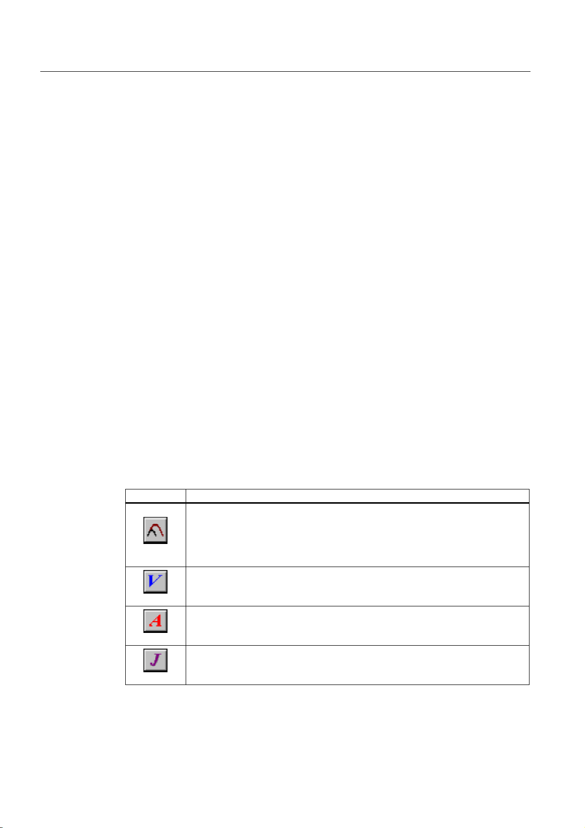
Table 3-1 SIMOTION CamTool toolbar icons

Symbol Explanation / instructions

With this icon, you can activate or deactivate the display of the scaled curve. If you have not specified a scaling, the icon is shown grayed-out.

Note:

If the scaled curve is displayed, you cannot edit the original curves in the diagram displays.

With this icon, you can show or hide the V diagram (velocity diagram).

With this icon, you can show or hide the A diagram (acceleration diagram).

With this icon, you can show or hide the J diagram (jerk diagram).

CamTool

3-2 Configuration Manual, 12.2004, 6AU1900-1AB32-0BA0

Configuring

3.2 Customizing the Working Area Display

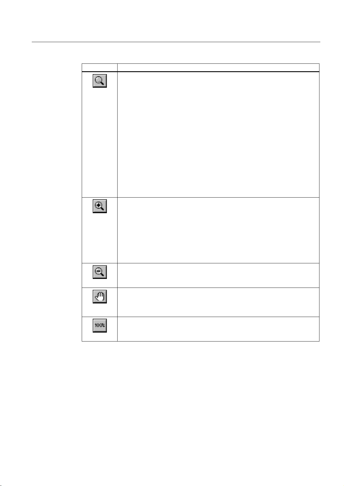
Symbol Explanation / instructions

With this icon, you can activate or deactivate the zoom tool. You can also deactivate the zoom tool using the ESC key.

You can perform various functions with the activated zoom tool. The function is dependent on whether the mouse pointer is on the diagram area or on a coordinate axis and whether the SHIFT key is also pressed:

Zoom tool on the diagram area (zoom in all directions at the same time)

Left-click to increase the size of the display by the factor 2.

Right-click to decrease the size of the display by the factor 2.

Zoom tool on the coordinate axis (zoom in all directions at the same time)

Left-click to increase the size of the display by the factor 2 in the direction of the coordinate axis on which you are pointing.

Right-click to decrease the size of the display by the factor 2 in the direction of the coordinate axis on which you are pointing.

Zoom tool with pressed SHIFT key

The mouse pointer is activated as a hand tool while you keep the SHIFT key pressed. With activated hand tool, you can move the diagram area with drag&drop. All displayed diagrams are adjusted to the move.

With this icon, you can activate or deactivate the zoom function. You can also deactivate the zoom function using the ESC key.

Zoom function on the diagram area

With activated zoom function, you can lasso a section of the diagram area that you want to enlarge with the mouse button pressed.

Zoom function on the coordinate axis

With activated zoom function, you can lasso a section of a coordinate axis that you want to enlarge with the mouse button pressed. The enlargement is in the direction in which you lasso the section of the coordinate axis.

With this icon, you can restore the previous zoom setting.

With this icon, you can activate or deactivate the hand tool. You can also deactivate the hand tool using the ESC key.

With activated hand tool, you can move the diagram area with drag&drop. All displayed diagrams are adjusted to the move.

With this icon, you can restore the whole display to the normal view.

CamTool Configuration Manual, 12.2004, 6AU1900-1AB32-0BA0

3-3

Configuring

3.2 Customizing the Working Area Display

3.2.2 Maximizing working area

Maximizing the working area

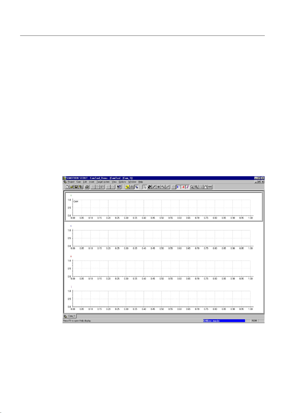
To set the largest possible working area for SIMOTION CamTool:

1. In the View menu, click Maximized working area. Detail view and project navigator are closed.

2. Maximize the window with the diagrams of the cam.

1. Close the project navigator via the menu View > Project navigator.

2. Close the detail view via the menu View > Detail view.

3. Maximize the window with the diagrams of the cam.

Figure 3-1 Maximized cam diagrams in the SIMOTION SCOUT working area

CamTool

3-4 Configuration Manual, 12.2004, 6AU1900-1AB32-0BA0

Configuring

3.3 Editing a Cam with CamTool

3.3.1 Content

Overview

With SIMOTION CamTool, you can edit a cam that is inserted in a SCOUT project.

You can use the following methods to insert and edit a cam. You can

• add a cam to a SCOUT project using SIMOTION CamTool.

• edit with CamTool a cam created with CamEdit.

• import and edit a cam from a text file.

• upload and edit a cam from a SIMOTION device.

3.3.2 Adding a cam to a SCOUT project using CamTool

Requirements

SIMOTION CamTool is installed as an option package for SIMOTION SCOUT.

The project, into which you want to insert the cam, is opened in SIMOTION SCOUT. At least one SIMOTION device is configured in this project.

CamTool Configuration Manual, 12.2004, 6AU1900-1AB32-0BA0

3-5

Configuring

3.3 Editing a Cam with CamTool

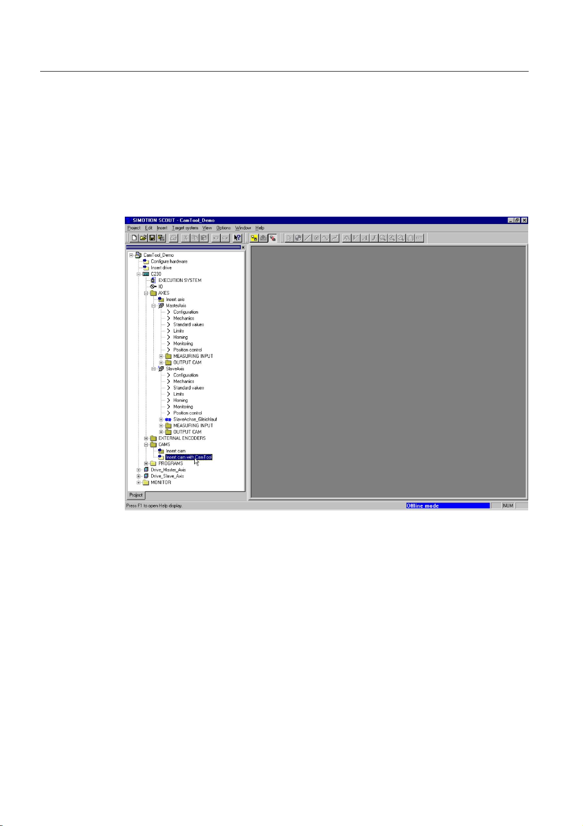
Inserting a cam in a SCOUT project

To insert a cam in a SCOUT project:

1. In the project navigator, find the SIMOTION device under which you want to insert a new cam.

2. Open the Cams folder and double-click Insert cam with CamTool.

Figure 3-2 Inserting a cam with CamTool

CamTool

3-6 Configuration Manual, 12.2004, 6AU1900-1AB32-0BA0

Configuring

3.3 Editing a Cam with CamTool

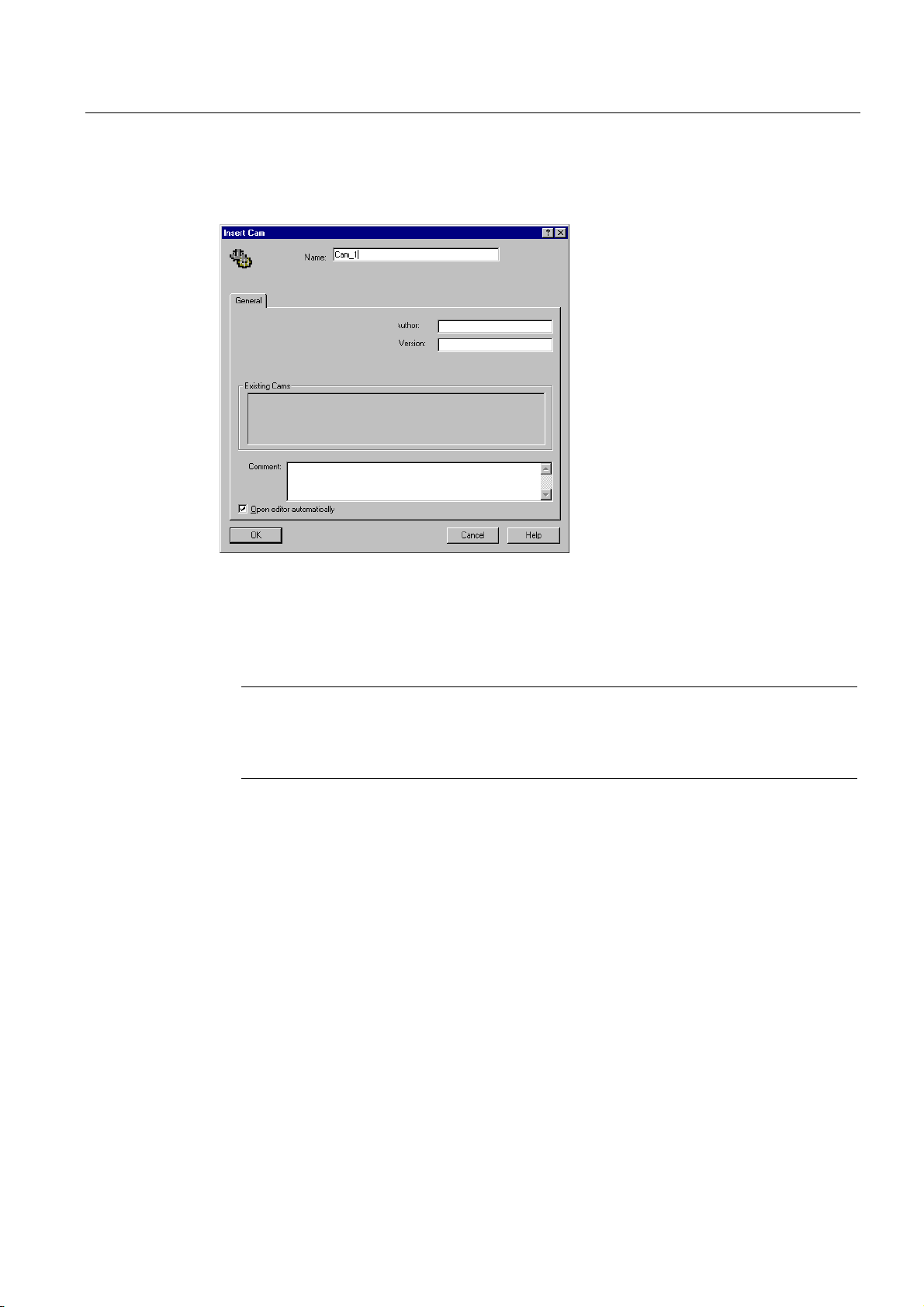
3. The Insert Cam window appears. Under Name, enter a unique name for the cam (all the

cams existing in the project are displayed under Existing cams).

Figure 3-3 Window for inserting a cam

4. Click OK. A window appears in the working area of SIMOTION SCOUT. The diagrams of

the cam depending on the settings in the menu Cam > Diagrams are displayed in this window.

Notice

The following are represented in the cam diagrams:

• the master axis in the horizontal direction (X-axis) and

• the slave axis in the vertical direction (Y-axis).

3.3.3 Edit cam created with CamEdit with CamTool

Editing a Cam with CamTool

To edit a cam created with CamEdit with CamTool:

1. Close the cam in SIMOTION CamEdit.

2. Find the cam that you want to edit with SIMOTION CamTool in the project navigator.

3. Right-click the cam and select Convert to CamTool in the displayed context menu. The

cam is then opened the next time with SIMOTION CamTool.

CamTool Configuration Manual, 12.2004, 6AU1900-1AB32-0BA0

3-7

Configuring

3.3 Editing a Cam with CamTool

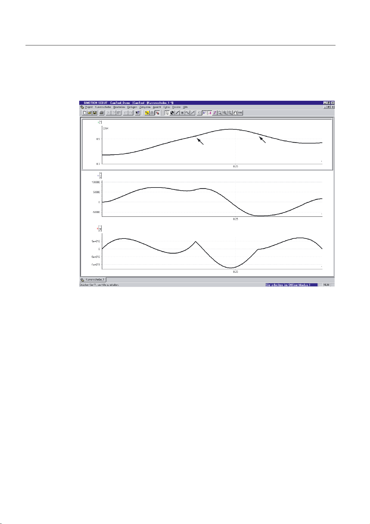
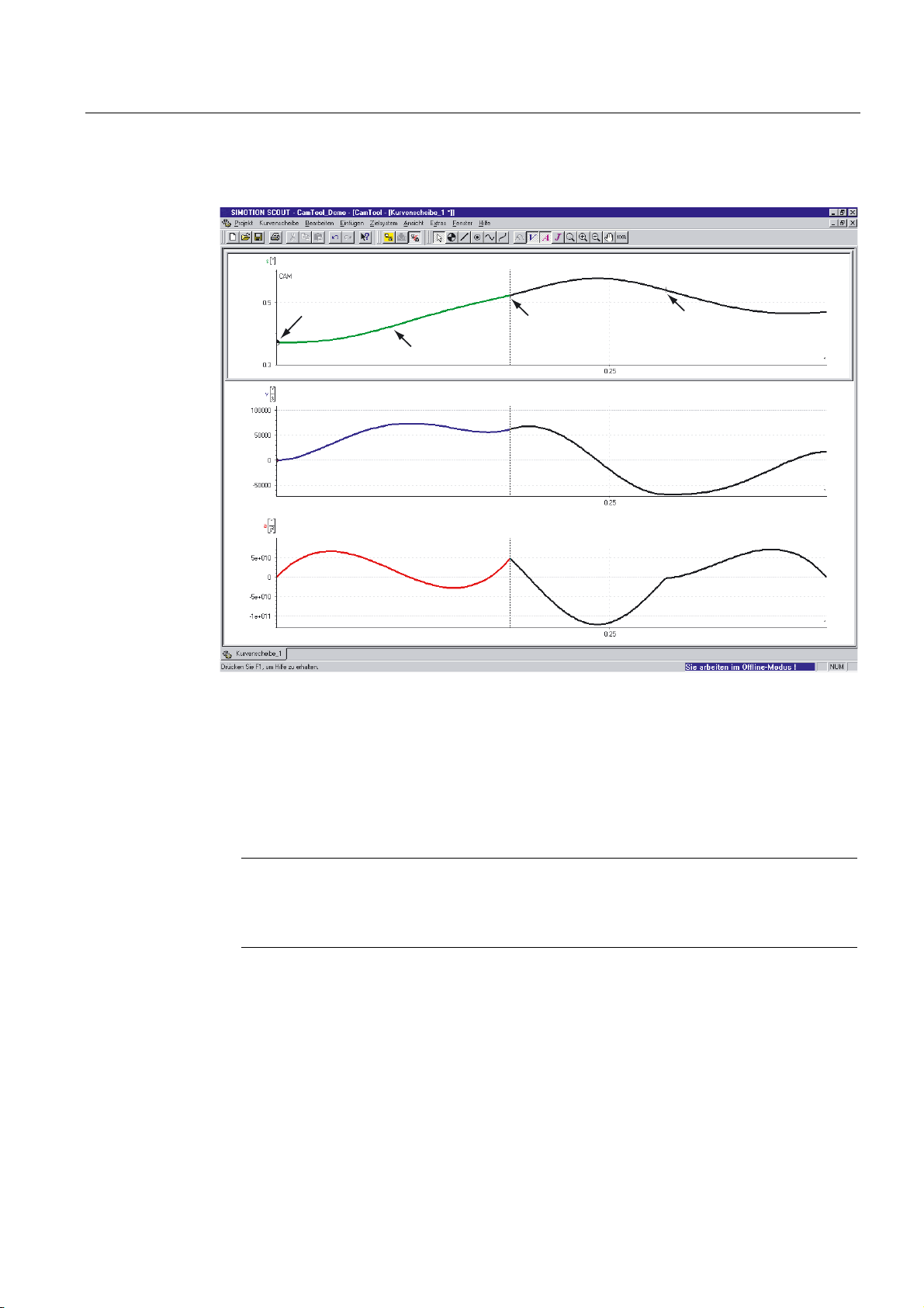
4. Double-click the cam. The cam is opened with SIMOTION CamTool and displayed. Segment limits between individual cam segments are marked in the S diagram (distance diagram).

6GLDJUDPGLVWDQFHGLDJUDP

6HJPHQWERXQGDU\

9GLDJUDPYHORFLW\GLDJUDP

6HJPHQWERXQGDU\

$GLDJUDPDFFHOHUDWLRQGLDJUDP

Figure 3-4 Open with CamTool a cam created with CamEdit

5. Select the cam segment that you want to edit. Note the displayed segment limits.

CamTool

3-8 Configuration Manual, 12.2004, 6AU1900-1AB32-0BA0

Configuring

3.3 Editing a Cam with CamTool

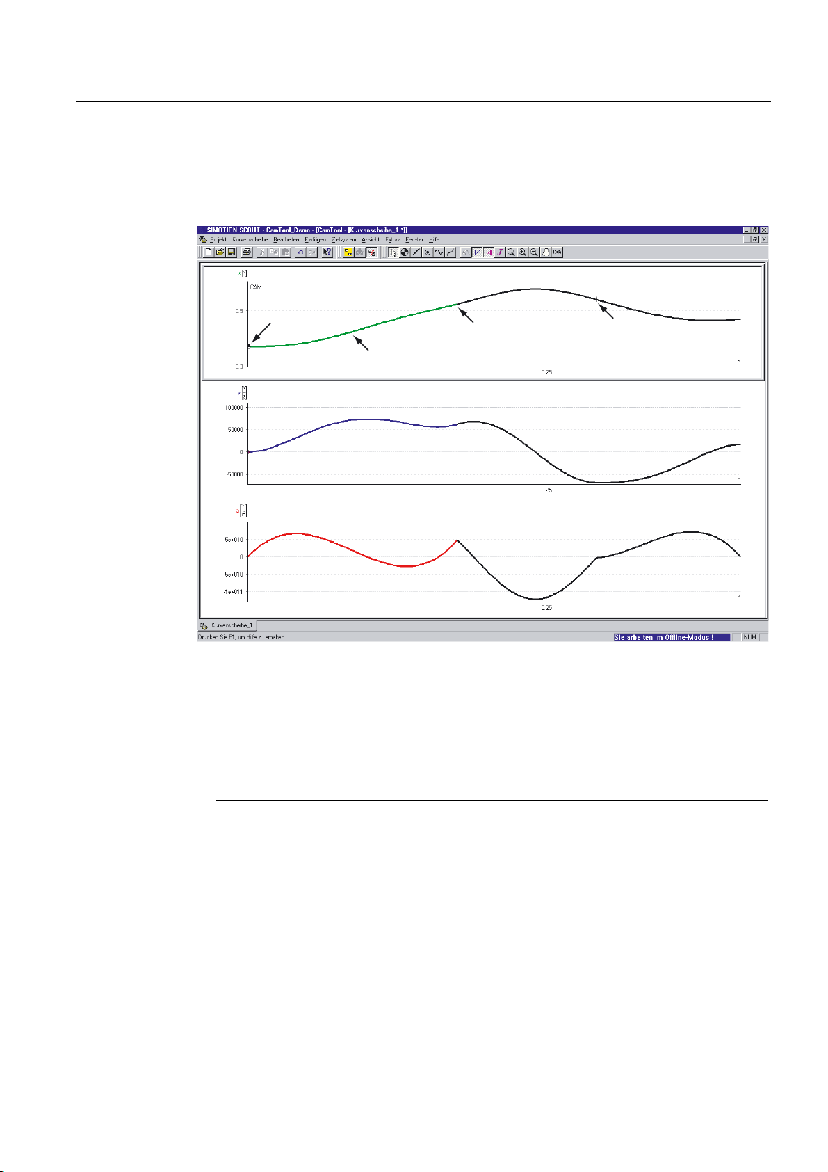
6. Delete the cam segment by pressing the DEL key. The cam segment is replaced by an

interpolation curve (transition) by SIMOTION CamTool. If required, fixed points are inserted in the curve to maintain the corner points of the original curve.

6GLDJUDPGLVWDQFHGLDJUDP

)L[HGSRLQW

6HJPHQWERXQGDU\

,QWHUSRODWLRQFXUYHWUDQVLWLRQ

9GLDJUDPYHORFLW\GLDJUDP

$GLDJUDPDFFHOHUDWLRQGLDJUDP

Figure 3-5 Cam segment replaced by SIMOTION CamTool with fixed point and transition

(interpolation polynomial)

6HJPHQWERXQGDU\

7. The cam segment (e.g. fixed point) inserted by SIMOTION CamTool can be edited (e.g.

change position).

8. The interpolation curve (transition) inserted by SIMOTION CamTool can be optimized

(e.g. velocity).

Notice

With SIMOTION CamTool, you can edit all cams created with SIMOTION CamEdit.

CamTool Configuration Manual, 12.2004, 6AU1900-1AB32-0BA0

3-9

Configuring

3.3 Editing a Cam with CamTool

3.3.4 Import cam from text file

Introduction

You can re-import a cam exported as text file from SIMOTION CamTool back into CamTool (e.g. to re-import a cam edited in an external program).

Importing a cam

Notice

The cam representation in the text file must correspond to the Microsoft Excel CSV format.

To import a cam from a text file:

1. Open with SIMOTION CamTool the cam in which you want to import the cam from the text file.

Add a new cam in which you want to import the cam from the text file.

6GLDJUDPGLVWDQFHGLDJUDP

6HJPHQWERXQGDU\

9GLDJUDPYHORFLW\GLDJUDP

$GLDJUDPDFFHOHUDWLRQGLDJUDP

Figure 3-6 Cam imported from a text file

CamTool

3-10 Configuration Manual, 12.2004, 6AU1900-1AB32-0BA0

Configuring

3.3 Editing a Cam with CamTool

2. Click a diagram to show the Cam menu.

6GLDJUDPGLVWDQFHGLDJUDP

)L[HGSRLQW

6HJPHQWERXQGDU\

,QWHUSRODWLRQFXUYHWUDQVLWLRQ

9GLDJUDPYHORFLW\GLDJUDP

$GLDJUDPDFFHOHUDWLRQGLDJUDP

Figure 3-7 Cam segment replaced by SIMOTION CamTool with fixed point and transition

(interpolation polynomial)

6HJPHQWERXQGDU\

3. Click the menu Cam > Import. The file selection window is displayed.

Navigate under Find in to the text file that contains the cam and select the text file. The name of the text file is entered under Name.

4. Click OK in the file selection window. The cam is imported.

Notice

When you import a cam from a text file and have previously changed the displayed cam, a window appears. You can accept the changed cam into the project via the window. The cam is then imported from the text file.

CamTool Configuration Manual, 12.2004, 6AU1900-1AB32-0BA0

3-11

Configuring

3.3 Editing a Cam with CamTool

Edit imported cam

To edit a cam imported into SIMOTION CamTool:

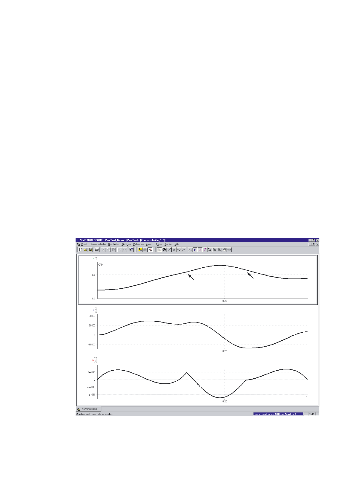
1. The cam imported from a text file is displayed in SIMOTION CamTool. Segment limits between individual cam segments are marked in the S diagram (distance diagram).

Select the cam segment that you want to edit. Note the displayed segment limits.

2. Delete the cam segment by pressing the DEL key. The cam segment is replaced by an interpolation curve (transition) by SIMOTION CamTool. If required, fixed points are inserted in the curve to maintain the corner points of the original curve.

3. The cam segment (e.g. fixed point) inserted by SIMOTION CamTool can be edited (e.g. change position).

4. The interpolation curve (transition) inserted by SIMOTION CamTool can be optimized (e.g. velocity).

3.3.5 Upload cam from SIMOTION device

Requirements

The cam is opened with SIMOTION CamTool.

Notice

If you create a cam and the cam has never been previously downloaded to the SIMOTION device, you must first download the entire configuration with the new cam to the SIMOTION device.

Only then can you upload the cam currently opened with SIMOTION CamTool from the SIMOTION device. The upload is only possible in ONLINE status.

CamTool

3-12 Configuration Manual, 12.2004, 6AU1900-1AB32-0BA0

Configuring

3.3 Editing a Cam with CamTool

Upload cam

To upload a cam from a SIMOTION device:

1. Click the menu Project > Connect to target system. The system changes to ONLINE

status.

6GLDJUDPGLVWDQFHGLDJUDP

6HJPHQWERXQGDU\

Figure 3-8 Cam uploaded from SIMOTION device

6HJPHQWERXQGDU\

9GLDJUDPYHORFLW\GLDJUDP

$GLDJUDPDFFHOHUDWLRQGLDJUDP

CamTool Configuration Manual, 12.2004, 6AU1900-1AB32-0BA0

3-13

Configuring

3.3 Editing a Cam with CamTool

2. Click a diagram to show the Cam menu.

6GLDJUDPGLVWDQFHGLDJUDP

)L[HGSRLQW

6HJPHQWERXQGDU\

,QWHUSRODWLRQFXUYHWUDQVLWLRQ

9GLDJUDPYHORFLW\GLDJUDP

$GLDJUDPDFFHOHUDWLRQGLDJUDP

Figure 3-9 Cam segment replaced by SIMOTION CamTool with fixed point and transition

(interpolation polynomial)

6HJPHQWERXQGDU\

3. Click the menu Cam > Upload cam. The cam is uploaded from the SIMOTION device.

4. After the upload, you can change back to OFFLINE status. Click the menu Project > Disconnect from target system.

Notice

When you upload a cam from the SIMOTION device and have previously changed the displayed cam, a window appears. You can accept the changed cam into the project via the window. The cam is then uploaded from the SIMOTION device.

CamTool

3-14 Configuration Manual, 12.2004, 6AU1900-1AB32-0BA0

Configuring

3.4 Save cam

Edit uploaded cam

To edit a cam uploaded from a SIMOTION device:

1. The uploaded cam is displayed in SIMOTION CamTool. Segment limits between

individual cam segments are marked in the S diagram (distance diagram).

Select the cam segment that you want to edit. Note the displayed segment limits.

2. Delete the cam segment by pressing the DEL key. The cam segment is replaced by an

interpolation curve (transition) by SIMOTION CamTool. If required, fixed points are inserted in the curve to maintain the corner points of the original curve.

3. The cam segment (e.g. fixed point) inserted by SIMOTION CamTool can be edited (e.g.

change position).

4. The interpolation curve (transition) inserted by SIMOTION CamTool can be optimized

(e.g. velocity).

3.4 Save cam

Requirements

Save cam

The cam is opened with SIMOTION CamTool.

Notice

When you exit SIMOTION CamTool and have previously changed the cam, a window appears. You can accept the changed cam into the project via the window. SIMOTION CamTool is then closed.

When you upload a cam from a SIMOTION device and have previously changed the displayed cam, a window appears. You can accept the changed cam into the project via the window. The cam is then uploaded from the SIMOTION device.

To save a cam:

1. Click the menu Project > Save. The cam is transferred to the SCOUT project.

CamTool Configuration Manual, 12.2004, 6AU1900-1AB32-0BA0

3-15

Configuring

3.5 Customize the display of the cam

3.5.1 Display the cam

Diagram display

The S diagram (distance diagram) of the cam is always displayed in the SIMOTION SCOUT working area. You can show or hide the V diagram (velocity diagram), the A diagram (acceleration diagram) and the J diagram (jerk diagram) via icons in the toolbar.

Representation parameters

You can customize the display parameters (e.g. representation range) for the master axis, the slave axis and the individual diagrams. This also includes the fonts and lines used for the display.

3.5.2 Show/hide diagram

Requirements

The cam is opened with SIMOTION CamTool.

Show/hide diagram

To show/hide a diagram:

1. Click a diagram to show the Cam menu.

CamTool

3-16 Configuration Manual, 12.2004, 6AU1900-1AB32-0BA0

Configuring

3.5 Customize the display of the cam

2. Click the diagram that you want to show or hide under menu Cam > Diagrams. The

diagram is shown or hidden.

Figure 3-10 Show/hide diagrams again

3.5.3 Change axis representation parameters

Requirements

The cam is opened with SIMOTION CamTool.

Change axis representation parameters

To change the representation parameters for the master or slave axis:

1. Click a diagram to show the Cam menu.

2. Click the axis whose representation parameters you want to change under

menu Cam > Representation parameters.

CamTool Configuration Manual, 12.2004, 6AU1900-1AB32-0BA0

3-17

Configuring

3.5 Customize the display of the cam

3. Either the window Master Properties (for the master axis) or the window S Diagram Properties (Slave) (for the slave axis) is displayed.

For the master axis, change the representation parameters in the window Master Properties.

Figure 3-11 Master Properties window

For the slave axis, change the representation parameters in the window S Diagram (Slave) Properties.

Figure 3-12 Slave Properties window

Table 3-2 Parameters in the Master Properties or S Diagram (Slave) Properties

Field/button Explanation/instructions

Master Range

(Master Properties)

Start Enter the start point of the curve, or the start of the master

End Enter the end point of the curve, or the end of the master

CamTool

You specify the master range (definition range) of the curve via start and end points. Cam segments must lie within this master range (see also Master range under Target device properties in the Coordinates tab).

range of the curve here.

3-18 Configuration Manual, 12.2004, 6AU1900-1AB32-0BA0

Configuring

3.5 Customize the display of the cam

Field/button Explanation/instructions

Representation range

Start

(Number of periods deactivated)

End

(Number of periods deactivated)

Number of periods

(cyclical absolute, cyclical relative)

Grid lines

Set automatically If you activate Set automatically, the grid lines will be

Main line spacing You can activate the display of the grid lines for the main

Auxiliary line spacing

(Main line spacing activated)

Specify here the Start point of the representation range.

If the Number of periods option has been activated, the system will determine the start point.

Specify here the End point of the representation range.

If the Number of periods option has been activated, the system will determine the end point.

If under Target device parameters in the Coordinates tab, you have specified the cyclic absolute execution type or the cyclic relative execution type, you can select the option Number of periods. Enter the number of periods that you want to display.

displayed automatically with an optimum spacing.

If you deactivate Set automatically, you can use Main line spacing or Auxiliary line spacing to specify the grid line spacing.

line spacing here.

If you deactivate the Set automatically option, you can specify the grid line spacing for the main line spacing.

Note:

The spacing that you specify for the grid lines in the main line spacing must be a multiple of the spacing that you specify for the grid lines in the auxiliary line spacing.

If the main line spacing option has been activated, you can also activate the display of the grid lines for the auxiliary line spacing.

If you deactivate the Set automatically option, you can specify the grid line spacing for the auxiliary line spacing.

Note:

The spacing that you specify for the grid lines in the main line spacing must be a multiple of the spacing that you specify for the grid lines in the auxiliary line spacing.

CamTool Configuration Manual, 12.2004, 6AU1900-1AB32-0BA0

3-19

Configuring

3.5 Customize the display of the cam

3.5.4 Change diagram representation parameters

Requirements

The cam is opened with SIMOTION CamTool.

Change diagram representation parameters

To change the representation parameters for the V diagram (velocity diagram), the A diagram (acceleration diagram) or the J diagram (jerk diagram):

1. Click a diagram to show the Cam menu.

2. Click the diagram whose representation parameters you want to change under menu Cam > Representation parameters.

3. Either the window V Diagram Properties (for the velocity diagram), the window A Diagram Properties (for the acceleration diagram) or the window J Diagram Properties (for the jerk diagram) is displayed.

For the V diagram (velocity diagram), change the representation parameters in the window V Diagram Properties.

Figure 3-13 V Diagram Properties window

For the A diagram (acceleration diagram), change the representation parameters in the window A Diagram Properties.

Figure 3-14 A Diagram Properties window

CamTool

3-20 Configuration Manual, 12.2004, 6AU1900-1AB32-0BA0

Configuring

3.5 Customize the display of the cam

For the J diagram (jerk diagram), change the representation parameters in the window J Diagram Properties.

Figure 3-15 J Diagram Properties window

Table 3-3 Parameters for the V, A or J Diagram Properties windows

Field/button Explanation/instructions

Representation range

Automatically If you activate Automatically, the representation range in the

Y-direction will be automatically changed to the value range of the displayed curve.

If you deactivate Automatically, you can use maximum value and minimum value to specify the representation range in the Y-direction.

Maximum value

(automatically deactivated)

Minimum value

(automatically deactivated)

Grid lines

Set automatically If you activate Set automatically, the grid lines will be

Main line spacing You can activate the display of the grid lines for the main

Specify here the maximum value of the representation range.

If the Automatically option has been activated, the system will determine the maximum value.

Specify here the minimum value of the representation range.

If the Automatically option has been activated, the system will determine the minimum value.

displayed automatically with an optimum spacing.

If you deactivate Set automatically, you can use Main line spacing or Auxiliary line spacing to specify the grid line spacing.

line spacing here.

If you deactivate the Set automatically option, you can specify the grid line spacing for the main line spacing.

Note:

The spacing that you specify for the grid lines in the main line spacing must be a multiple of the spacing that you specify for the grid lines in the auxiliary line spacing.

CamTool Configuration Manual, 12.2004, 6AU1900-1AB32-0BA0

3-21

Configuring

3.5 Customize the display of the cam

Field/button Explanation/instructions

Auxiliary line spacing

(Main line spacing activated)

If the main line spacing option has been activated, you can also activate the display of the grid lines for the auxiliary line spacing.

If you deactivate the Set automatically option, you can specify the grid line spacing for the auxiliary line spacing.

Note:

The spacing that you specify for the grid lines in the main line spacing must be a multiple of the spacing that you specify for the grid lines in the auxiliary line spacing.

3.5.5 Change lines and fonts representation parameters

For the representation of the diagrams, default parameters are used for the lines and fonts. You can change these default settings.

/LQHIRUFDPVHJPHQWV

/LQHIRUVLPXODWHGLQWHUSRODWLRQ

<FRRUGLQDWHD[LV

;FRRUGLQDWHD[LV

$X[LOLDU\OLQH

,QWHUSRODWLRQFXUYHLQWKHGLVWDQFHGLDJUDP

$X[LOLDU\JULGOLQHV

0DLQJULGOLQH

9HORFLW\FXUYH

$X[LOLDU\OLQH

$FFHOHUDWLRQFXUYH

-HUNFXUYH

/LQHDWSK\VLFDOOLPLW

Figure 3-16 Representation parameters in the diagrams (line for the scaling not shown)

CamTool

3-22 Configuration Manual, 12.2004, 6AU1900-1AB32-0BA0

Configuring

3.5 Customize the display of the cam

Table 3-4 Representation parameters in the diagrams

Representation parameters Note

Main grid line Type and color of the line can be changed.

Auxiliary grid lines Type and color of the line can be changed.

Auxiliary line Type, color and width of the line can be changed.

Line at physical limit Type, color and width of the line can be changed.

X-coordinate axis Color and width of the line can be changed.

Y-coordinate axis Color and width of the line can be changed.

Line for simulated interpolation Color and width of the line can be changed.

The line for simulated interpolation is used to display a transition interpolated by the target device.

Interpolation curve in the distance diagram Color and width of the line can be changed.

Velocity curve Color and width of the line can be changed.

Acceleration curve Color and width of the line can be changed.

Jerk curve Color and width of the line can be changed.

Line for cam segments Color and width of the line can be changed.

Line for scaling Color and width of the line can be changed.

The line for scaling is used to display a scaled and offset curve.

Requirements

The cam is opened with SIMOTION CamTool.

Change lines and fonts representation parameters

To change the representation parameters for lines and fonts:

1. Click a diagram to show the Cam menu.

2. Click Lines and fonts under menu Cam > Representation parameters.

3. The Lines and Fonts window appears.

You can change the representation parameters for the lines in the Line tab.

Table 3-5 Parameters in the Line tab

Field/button Explanation/instructions

Line type Select the line type that you want to specify here.

Settings Note:

Type Specify the type of the line.

Under Settings, the associated parameters are displayed and the line type shown.

Grayed-out parameters cannot be changed.

The line type is displayed in the Preview.

CamTool Configuration Manual, 12.2004, 6AU1900-1AB32-0BA0

3-23

Configuring

3.5 Customize the display of the cam

Field/button Explanation/instructions

Color Specify the color of the line.

The line is displayed in the Preview.

Width Specify the thickness of the line.

The line type is displayed in the Preview.

Preview Under Preview, the line type specified via type, color and

width is shown.

You can change the representation parameters for the fonts in the Font tab.

Table 3-6 Parameters in the Font tab

Field/button Explanation/instructions

Settings

Font Select the font here.

The font is displayed in the Preview.

Font style Select the font style here.

The font is displayed in the Preview.

Font size Select the font size here.

The font is displayed in the Preview.

Preview Under Preview, the font specified via font, font style and font

size is shown.

3.5.6 Displaying auxiliary lines in the diagram

You can represent horizontal and vertical auxiliary lines in the individual diagrams. You can, for example, determine the position of individual points of the curve via auxiliary lines.

Requirements

The cam is opened with SIMOTION CamTool.

Representing a horizontal auxiliary line in a diagram

To represent a horizontal auxiliary line (in the direction of the x-coordinate) in a diagram:

1. Click in the diagram, in which you want to represent a horizontal auxiliary line, on the xcoordinate and keep the mouse button pressed. The current position of the auxiliary line is displayed in the position window.

CamTool

3-24 Configuration Manual, 12.2004, 6AU1900-1AB32-0BA0

Configuring

3.5 Customize the display of the cam

2. Drag the auxiliary line to the position at which you want to represent the auxiliary line and

release the mouse button. The auxiliary line and the position window with the current position are displayed in the diagram.

Figure 3-17 Displaying a horizontal auxiliary line

Representing vertical auxiliary lines in all displayed diagrams

To represent a vertical auxiliary line (in the direction of the y-coordinate) in all displayed diagrams:

1. Click in a diagram on the y-coordinate axis and keep the mouse button pressed. The

current position of the auxiliary line is displayed in the position window.

2. Drag the auxiliary line to the position at which you want to represent the auxiliary line and

release the mouse button. The auxiliary line and the position window with the current position are both displayed in all the displayed diagrams.

Figure 3-18 Displaying a vertical auxiliary line

CamTool Configuration Manual, 12.2004, 6AU1900-1AB32-0BA0

3-25

Configuring

3.6 Download cam to SIMOTION device

Moving the position window along an auxiliary line

To move a position window with the current position of the auxiliary line along the horizontal or vertical auxiliary line:

1. Point at the position window. The mouse pointer shows the direction in which you can move the window. Drag the window with the current position with drag&drop to the new position.

Figure 3-19 Moving the position window horizontally

Deleting an auxiliary line in a diagram

To delete a horizontal or vertical auxiliary line in a diagram:

1. Select the auxiliary line that you want to delete.

2. Press the DEL key. The auxiliary line is deleted.

3.6 Download cam to SIMOTION device

Requirements

The cam is opened with SIMOTION CamTool.

Notice

If you create a cam and the cam has never been previously downloaded to the SIMOTION device, you must first download the entire configuration with the new cam to the SIMOTION device.

Only then can you download the cam independent of the other technology objects in the SIMOTION device. The download is only possible in ONLINE status.

CamTool

3-26 Configuration Manual, 12.2004, 6AU1900-1AB32-0BA0

Configuring

3.6 Download cam to SIMOTION device

Download cam to SIMOTION device

To download a cam to a SIMOTION device:

1. Click the menu Project > Connect to target system. The system changes to ONLINE

status.

2. Click a diagram to show the Cam menu.

3. Click the menu Cam > Download cam. The cam is downloaded to the SIMOTION device.

4. After the download, you can change back to OFFLINE status. Click the menu

Project > Disconnect from target system.

CamTool Configuration Manual, 12.2004, 6AU1900-1AB32-0BA0

3-27

Functions

4.1 Content

Overview

In this chapter you learn how you can use SIMOTION CamTool to create and optimize a cam, and to make the simulation settings. In addition, you learn how you can use CamTool to edit a cam created with CamEdit and how you can export a cam as a text file.

Note

The following operating instructions primarily describe the operation of SIMOTION CamTool using the functions in the menu bar.

You can also execute the functions from the context menus. In this case, right-click the element that you want to edit.

You can also execute the most import functions using the icons in the SIMOTION CamTool toolbar. Pay attention to the Tooltip which is displayed when you place the mouse pointer on an icon in the toolbar.

CamTool Configuration Manual, 12.2004, 6AU1900-1AB32-0BA0

4-1

Functions

4.2 Structure of a cam

Introduction

Create the cam in the S diagram (distance diagram). The curve represents the path-related dependency between the master axis (X-axis in the diagram) and the slave axis (Y-axis in the diagram).

Structure of a cam

The cam consists of individual cam segments.

Under SIMOTION CamTool, you can use fixed points, straight lines, sine curves, arc sine curves and interpolation points as cam segments.

SIMOTION CamTool calculates interpolation curves between the individual cam segments and displays the V diagram (velocity diagram), the A diagram (acceleration diagram) and the J diagram (jerk diagram).

6WUDLJKWOLQH

)L[HGSRLQW

,QWHUSRODWLRQFXUYH

6WUDLJKWOLQH

6GLDJUDPGLVWDQFHGLDJUDP

,QWHUSRODWLRQFXUYH

Interpolation curve

9GLDJUDPYHORFLW\GLDJUDP

$GLDJUDPDFFHOHUDWLRQGLDJUDP

-GLDJUDPMHUNGLDJUDP

Figure 4-1 Example of a cam with interpolation curves

CamTool

4-2 Configuration Manual, 12.2004, 6AU1900-1AB32-0BA0

Functions

4.3 Fixed point

4.3.1 Fixed Point Definition

Definition

The cam consists of individual cam segments. Under SIMOTION CamTool, you can use fixed points, straight lines, sine curves, arc sine curves and interpolation points as cam segments.

A fixed point is a specified position of the slave axis for a certain position of the master axis. You can specify the velocity and acceleration at the fixed point position.

Notice

With a fixed point, you define a single fixed position. The transitions between adjacent cam segments are optimally calculated by CamTool.

If you want to specify an arbitrary characteristic, you must use interpolation points. The individual interpolation points are connected by CamTool with cubic splines in order to generate a curve specified by the interpolation points which is as exact as possible.

4.3.2 Insert fixed point

Requirements

The cam is opened with SIMOTION CamTool.

Insert fixed point

To insert a fixed point:

1. Click in the S diagram (distance diagram) to activate the diagram.

2. Click under menu Cam > Insert at fixed point. The mouse pointer changes.

3. With the changed mouse pointer, click the position in the S diagram (distance diagram) at

which you want to insert the fixed point.

CamTool Configuration Manual, 12.2004, 6AU1900-1AB32-0BA0

4-3

Functions

4.3 Fixed point

The fixed point is displayed in the diagram. The position of the fixed point shown in the tooltip.

Figure 4-2 Insert fixed point

Notice

Once the function Cam > Insert > Fixed point is activated, you can insert fixed points in the S diagram (distance diagram) until

• you press the ESC key,

• you press the right mouse button (this activates the selection tool in the toolbar) or

• you activate another cam segment (straight line, sine curve, arc sine curve, interpolation point)

for insertion.

CamTool

4-4 Configuration Manual, 12.2004, 6AU1900-1AB32-0BA0

Functions

4.3 Fixed point

4.3.3 Change fixed point position

Requirements

The cam is opened with SIMOTION CamTool.

Change fixed point position

To change the position of a fixed point:

1. Select the fixed point in the S diagram (distance diagram). The position of the fixed point

shown in the tooltip.

2. Move the fixed point with drag&drop to the new position.

1. Double-click the fixed point. The Fixed Point Properties window appears.

2. Enter the new x- or y-position of the fixed point in the Position tab and click OK. The

representation of the fixed point in the diagram will be updated and displayed at the new position.

4.3.4 Changing the velocity at the position of a fixed point:

Requirements

The cam is opened with SIMOTION CamTool.

Change velocity at fixed point

To change the velocity at the fixed point position:

1. The velocity at a fixed point position is represented by a handle in the V diagram (velocity

diagram).

Select the handle. The mouse pointer shows the direction in which you can move the handle.

2. Move the handle with drag&drop to the new position.

1. Double-click the fixed point. The Fixed Point Properties window appears.

2. Enter the new velocity as specified in the following table in the Dynamic response tab and

click OK. The handle in the V diagram (velocity diagram) is shown at the new position.

CamTool Configuration Manual, 12.2004, 6AU1900-1AB32-0BA0

4-5

Functions

4.3 Fixed point

Field/button Explanation/instructions

v = Under v =, the current velocity at the position of the fixed point is

displayed.

(see note below)

a =

(manual input activated)

Manual input If you activate Manual input, you can enter an acceleration value

Under a =, the current acceleration at the position of the fixed point is displayed.

If Manual input is deactivated, the acceleration value is calculated by the system. The jerk diagram (J diagram) is smooth at the position of the fixed point.

If Manual input is activated, you can enter an acceleration value. To change the acceleration, enter the new acceleration under a = and click Accept or OK. The display of the fixed point in the diagrams is refreshed.

under a =.

If you deactivate Manual input, the acceleration value is calculated by the system. The jerk diagram (J diagram) is smooth at the position of the fixed point.

Notice

To specify an absolute slave velocity, you must select an absolute master velocity for calculations in the Simulation Settings window.

4.3.5 Changing the acceleration at a fixed point position:

Requirements

The cam is opened with SIMOTION CamTool.

Change acceleration at fixed point

To change the acceleration at the fixed point position:

1. Right-click the fixed point and select Direct entry for acceleration in the displayed context menu.

2. The acceleration at a fixed point position is represented by a handle in the A diagram (acceleration diagram).

Select the handle. The mouse pointer shows the direction in which you can move the handle.

3. Move the handle with drag&drop to the new position.

CamTool

4-6 Configuration Manual, 12.2004, 6AU1900-1AB32-0BA0

Functions

4.4 Straight line

1. Double-click the fixed point. The Fixed Point Properties window appears.

2. In the Dynamic response tab, activate the option Manual input and enter the new

acceleration.

3. Click OK. The handle in the A diagram (acceleration diagram) is shown at the new

position.

Notice

To specify an absolute slave acceleration, you must select an absolute master velocity for calculations in the Simulation Settings window.

4.3.6 Delete fixed point

Requirements

The cam is opened with SIMOTION CamTool.

Delete fixed point

To delete a fixed point:

1. Select the fixed point that you want to delete.

2. Press the DEL key. The fixed point is deleted and the representation of the cam adjusted

in all diagrams.

4.4 Straight line

4.4.1 Definition straight line

Definition

The cam consists of individual cam segments. Under SIMOTION CamTool, you can use fixed points, straight lines, sine curves, arc sine curves and interpolation points as cam segments.

A straight line defines a synchronous distance in the cam. You can specify the velocity along the straight line.

CamTool Configuration Manual, 12.2004, 6AU1900-1AB32-0BA0

4-7

Functions

4.4 Straight line

4.4.2 Insert straight line

Requirements

The cam is opened with SIMOTION CamTool.

Insert straight line

To insert a straight line:

1. Click in the S diagram (distance diagram) to activate the diagram.

2. Click Straight line under menu Cam > Insert. The mouse pointer changes.

With the changed mouse pointer, click the position in the S diagram (distance diagram) at which you want to insert the straight line. The straight line is inserted with a default size.

The current position of the straight line is shown in the tooltip.

Figure 4-3 Insert straight line

CamTool

4-8 Configuration Manual, 12.2004, 6AU1900-1AB32-0BA0

Functions

4.4 Straight line

Notice

Once the function Cam > Insert > Straight line is activated, you can insert straight lines in the S diagram (distance diagram) until

• you press the ESC key,

• you press the right mouse button (this activates the selection tool in the toolbar) or

• you activate another cam segment (fixed point, sine curve, arc sine curve, interpolation point)

for insertion.

4.4.3 Change straight line position

Requirements

The cam is opened with SIMOTION CamTool.

Change straight line position

To change the position of a straight line:

1. Select the straight line in the S diagram (distance diagram). The position of the straight

line is shown in the tooltip.

2. The straight line is shown with handles. Move the handles of the straight line with

drag&drop to the new positions.

1. Select the straight line in the S diagram (distance diagram). The position of the straight

line is shown in the tooltip.

2. Move the whole straight line with drag&drop to the new position.

Figure 4-4 Change the position of all straight lines

1. Double-click the straight line. The Straight Line Properties window appears.

2. Enter the new positions in the Position tab (left: x1 and y1, right: x2 and y2), and click OK.

The representation of the straight lines in the diagram will be updated and displayed at the new positions.

CamTool Configuration Manual, 12.2004, 6AU1900-1AB32-0BA0

4-9

Functions

4.4 Straight line

4.4.4 Changing the velocity along a straight line

Requirements

The cam is opened with SIMOTION CamTool.

Change velocity along a straight line

To change the velocity along a straight line:

1. The velocity along a straight line is represented by a line in the V diagram (velocity diagram).

Select the line. The mouse pointer shows the direction in which you can move the line.

2. Move the line with drag&drop to the new position. The S diagram (distance diagram) is automatically adjusted.

Figure 4-5 Changing the velocity along a straight line

1. Double-click the straight line. The Straight Line Properties window appears.

2. Enter the new velocity in the Dynamic response tab and click OK. The line in the V diagram (velocity diagram) is shown at the new position. The S diagram (distance diagram) is automatically adjusted.

Notice

To specify an absolute slave velocity, you must select an absolute master velocity for calculations in the Simulation Settings window.

CamTool

4-10 Configuration Manual, 12.2004, 6AU1900-1AB32-0BA0

Functions

4.5 Sine curve

4.4.5 Delete straight line

Requirements

The cam is opened with SIMOTION CamTool.

Deleting a straight line

To delete a straight line:

1. Select the straight line that you want to delete.

2. Press the DEL key. The straight line is deleted and the representation of the cam

adjusted in all diagrams.

4.5 Sine curve

4.5.1 Insert sine curve

Requirements

The cam is opened with SIMOTION CamTool.

Insert sine curve

To insert a sine curve:

1. Click in the S diagram (distance diagram) to activate the diagram.

2. Click Sine under menu Cam > Insert > Functions. The mouse pointer changes.

3. With the changed mouse pointer, click the position in the S diagram (distance diagram) at

which you want to insert the sine curve. The sine curve is inserted with a default size.

CamTool Configuration Manual, 12.2004, 6AU1900-1AB32-0BA0

4-11

Functions

4.5 Sine curve

The current position of the sine curve is shown in the tooltip.

Figure 4-6 Insert sine curve

Notice

Once the function Cam > Insert > Sine is activated, you can insert sine curves in the S diagram (distance diagram) until

• you press the ESC key,

• you press the right mouse button (this activates the selection tool in the toolbar) or

• you activate another cam segment (fixed point, straight line, arc sine curve, interpolation point)

for insertion.

CamTool

4-12 Configuration Manual, 12.2004, 6AU1900-1AB32-0BA0

Functions

4.5 Sine curve

4.5.2 Change sine curve position

Requirements

The cam is opened with SIMOTION CamTool.

Change sine curve position

To change the position of a sine curve:

1. Select the sine curve in the S diagram (distance diagram).

The current position of the sine curve is shown in the tooltip.

2. The sine curve is shown with handles. Point to a handle. The mouse pointer shows the

direction in which you can move the handle.

3. Move the handles with drag&drop to the new positions.

Figure 4-7 Change sine curve position

1. Select the sine curve in the S diagram (distance diagram).

The current position of the sine curve is shown in the tooltip.

2. Move the whole sine curve with drag&drop to the new position.

Figure 4-8 Changing the position of the complete sine curve

1. Double-click the sine curve. The Fx Sine Properties window appears.

CamTool Configuration Manual, 12.2004, 6AU1900-1AB32-0BA0

4-13

Functions

4.5 Sine curve

2. Enter the new position in the Position tab and click OK. The sine curve is shown at the new position.

Figure 4-9 Position (Fx Sine Properties) tab

4.5.3 Change sine curve definition range

Requirements

The cam is opened with SIMOTION CamTool.

Change sine curve definition range

To change the definition range of a sine curve:

1. Select the sine curve in the S diagram (distance diagram).

The current position of the sine curve is shown in the tooltip.

2. The sine curve is shown with handles. The handles for the definition range are shown in green. Point to a green handle. The mouse pointer shows the direction in which you can move the handle.

3. Move the green handles with drag&drop to the new positions. While moving, the current value of the respective limit of the definition range is displayed in the tooltip.

Figure 4-10 Change sine curve definition range

CamTool

4-14 Configuration Manual, 12.2004, 6AU1900-1AB32-0BA0

Functions

4.6 Arc Sine Curve

4.5.4 Delete sine curve

Requirements

The cam is opened with SIMOTION CamTool.

Delete sine curve

To delete a sine curve:

1. Select the sine curve that you want to delete.

2. Press the DEL key. The sine curve is deleted and the representation of the cam adjusted

in all diagrams.

4.6 Arc Sine Curve

4.6.1 Insert arc sine curve

Requirements

The cam is opened with SIMOTION CamTool.

Notice

The arc sine curve is calculated as an interpolation point table. The number of interpolation points can be specified in the Fx Arc Sine Properties window. Double-click the arc sine curve to show the window.

Insert arc sine curve

To insert an arc sine curve:

1. Click in the S diagram (distance diagram) to activate the diagram.

2. Click Arc sine under menu Cam > Insert > Functions. The mouse pointer changes.

3. With the changed mouse pointer, click the position in the S diagram (distance diagram) at

which you want to insert the arc sine curve. The arc sine curve is inserted with a default size.

CamTool Configuration Manual, 12.2004, 6AU1900-1AB32-0BA0

4-15

Functions

4.6 Arc Sine Curve

The current position of the arc sine curve is shown in the tooltip.

Figure 4-11 Insert arc sine curve

Notice

Once the function Cam > Insert > Arc sine is activated, you can insert arc sine curves in the S diagram (distance diagram) until

• you press the ESC key,

• you press the right mouse button (this activates the selection tool in the toolbar) or

• you activate another cam segment (fixed point, straight line, sine curve, interpolation point) for

insertion.

CamTool

4-16 Configuration Manual, 12.2004, 6AU1900-1AB32-0BA0

Functions

4.6 Arc Sine Curve

4.6.2 Change arc sine curve position

Requirements

The cam is opened with SIMOTION CamTool.

Change arc sine curve position

To change the position of an arc sine curve:

1. Select the arc sine curve in the S diagram (distance diagram).

The current position of the arc sine curve is shown in the tooltip.

2. The arc sine curve is shown with handles. Point to a handle. The mouse pointer shows

the direction in which you can move the handle.

3. Move the handles with drag&drop to the new positions.

Figure 4-12 Change arc sine curve position

1. Select the arc sine curve in the S diagram (distance diagram).

The current position of the arc sine curve is shown in the tooltip.

2. Move the whole arc sine curve with drag&drop to the new position.

Figure 4-13 Changing the position of the complete arc sine curve

1. Double-click the sine curve.

The Fx Arc Sine Properties window appears.

CamTool Configuration Manual, 12.2004, 6AU1900-1AB32-0BA0

4-17

Functions

4.6 Arc Sine Curve

2. Enter the new position and the number of interpolation points in the Position tab and click OK. The arc sine curve is shown at the new positions. The arc sine curve is saved by the system as an interpolation point table.

Figure 4-14 Position tab

4.6.3 Change arc sine curve definition range

Requirements

The cam is opened with SIMOTION CamTool.

Change arc sine curve definition range

To change the definition range of an arc sine curve:

1. Select the arc sine curve in the S diagram (distance diagram).

The current position of the arc sine curve is shown in the tooltip.

2. The arc sine curve is shown with handles. The handles for the definition range are shown in green. Point to a green handle. The mouse pointer shows the direction in which you can move the handle.

CamTool

4-18 Configuration Manual, 12.2004, 6AU1900-1AB32-0BA0

Functions

4.6 Arc Sine Curve

3. Move the green handles with drag&drop to the new positions. While moving, the current

value of the respective limit of the definition range is displayed in the tooltip.

Figure 4-15 Change arc sine curve definition range

4.6.4 Delete arc sine curve

Requirements

The cam is opened with SIMOTION CamTool.

Delete arc sine curve

To delete an arc sine curve:

1. Select the arc sine curve that you want to delete.

2. Press the DEL key. The arc sine curve is deleted and the representation of the cam

adjusted in all diagrams.

CamTool Configuration Manual, 12.2004, 6AU1900-1AB32-0BA0

4-19

Functions

4.7 Interpolation point

4.7.1 Interpolation Point Definition

Definition

The cam consists of individual cam segments. Under SIMOTION CamTool, you can use fixed points, straight lines, sine curves, arc sine curves and interpolation points as cam segments.

An interpolation point is a specified position in the S diagram (distance diagram).

4.7.2 Insert interpolation point

Requirements

The cam is opened with SIMOTION CamTool.

Notice

With a fixed point, you define a single fixed position. The transitions between adjacent cam segments are optimally calculated by CamTool.

If you want to specify an arbitrary characteristic, you must use interpolation points. The interpolation points are connected by CamTool with cubic splines in order to generate a curve specified by the interpolation points which is as exact as possible.

Insert interpolation point

To insert an interpolation point:

1. Click in the S diagram (distance diagram) to activate the diagram.

2. Click Interpolation point under menu Cam > Insert. The mouse pointer changes.

3. With the changed mouse pointer, click the position in the S diagram (distance diagram) at which you want to insert the interpolation point.

CamTool

4-20 Configuration Manual, 12.2004, 6AU1900-1AB32-0BA0

Functions

4.7 Interpolation point

The interpolation point is displayed in the diagram. The position of the interpolation point is shown in the tooltip.

Figure 4-16 Insert interpolation point

Notice

Once the function Cam > Insert > Interpolation point is activated, you can insert interpolation points in the S diagram (distance diagram) until

• you press the ESC key,

• you press the right mouse button (this activates the selection tool in the toolbar) or

• you activate another cam segment (fixed point, straight line, sine curve, arc sine curve) for

insertion.

4.7.3 Changing the interpolation point position

Requirements

The cam is opened with SIMOTION CamTool.

CamTool Configuration Manual, 12.2004, 6AU1900-1AB32-0BA0

4-21

Functions

4.7 Interpolation point

Changing an Interpolation Point Position

To change the position of an interpolation point:

1. Select the interpolation point in the S diagram (distance diagram). The position of the interpolation point is shown in the tooltip.

2. Move the interpolation point with drag&drop to the new position.

1. Double-click the interpolation point. The Interpolation Point Properties window appears.

2. Enter the new position in the Position tab and click OK. The interpolation point is displayed at the new position.

Figure 4-17 Position tab

4.7.4 Delete interpolation point

Requirements

The cam is opened with SIMOTION CamTool.

Delete interpolation point

To delete an interpolation point:

1. Select the interpolation point that you want to delete.

2. Press the DEL key. The interpolation point is deleted and the representation of the cam adjusted in all diagrams.

CamTool

4-22 Configuration Manual, 12.2004, 6AU1900-1AB32-0BA0

Functions

4.8 Optimizing a Cam

4.8.1 Optimizing a Cam

Introduction

Create the cam in the S diagram (distance diagram). The curve represents the path-related dependency between the master axis (X-axis in the diagram) and the slave axis (Y-axis in the diagram).

Structure of a cam

The cam consists of individual cam segments.

Under SIMOTION CamTool, you can use fixed points, straight lines, sine curves, arc sine curves and interpolation points as cam segments.

6WUDLJKWOLQH

)L[HGSRLQW

,QWHUSRODWLRQFXUYH

Figure 4-18 Example of a cam with interpolation curves

6WUDLJKWOLQH

6GLDJUDPGLVWDQFHGLDJUDP

,QWHUSRODWLRQFXUYH

Interpolation curve

9GLDJUDPYHORFLW\GLDJUDP

$GLDJUDPDFFHOHUDWLRQGLDJUDP

-GLDJUDPMHUNGLDJUDP

CamTool Configuration Manual, 12.2004, 6AU1900-1AB32-0BA0

4-23

Functions

4.8 Optimizing a Cam

4.8.2 Optimize transition

Requirements

The cam is opened with SIMOTION CamTool.

Optimize transition

To optimize a transition:

1. Right-click the transition that you want to optimize and select Properties in the displayed context menu.

Figure 4-19 Selecting the transition to be optimized

2. The Interpolation Curve Properties window appears. Specify the parameters in the Type tab.

3. Click the Parameters tab and specify the parameters.

CamTool

4-24 Configuration Manual, 12.2004, 6AU1900-1AB32-0BA0

Functions

4.8 Optimizing a Cam

4. Click the Limits tab to display the minimum and maximum values of the interpolation

curve.

Notice

For the slave axis, you can take over the settings of an axis already existing in the project via the menu Cam > Simulation settings and specify the limits of the axis. These simulation settings for the slave axis are used for the calculation of the percentage values which are displayed in the Limits tab.

1. Use the handles, which are dependent on the settings in the Interpolation Curve

Properties window, to optimize the cam.

2. The mouse pointer shows the direction in which you can move the handle.

3. Move the handle with drag&drop to the new position. The display of the cam is adjusted

in all diagrams.

Figure 4-20 Optimizing a cam with handle using drag&drop

CamTool Configuration Manual, 12.2004, 6AU1900-1AB32-0BA0

4-25

Functions

4.8 Optimizing a Cam

4.8.3 Interpolation Curve properties

Type

You can specify the type of the interpolation curve for the transition here.

You can set the following parameters:

Table 4-1 Parameters in the Type tab (Interpolation Curve Properties window)

Field/button Explanation/instructions

Transition The type of transition is displayed here.

Allow interpolation by target device If you activate this option, the system does not generate an interpolation

curve. The transition is interpolated by the target device. The representation of the transition is refreshed in the diagrams when you click Accept or OK.

Optimize for

(allow interpolation by target device deactivated)

Do not optimize If you select this option, all the interpolation curves which are suitable for

Velocity If you select this option, all the interpolation curves which are suitable for

Acceleration If you select this option, all the interpolation curves which are suitable for

Jerk If you select this option, all the interpolation curves which are suitable for

Applicable motion rules

(allow interpolation by target device deactivated)

the transition are displayed under Applicable motion rules.

the transition for the optimization of the velocity are displayed under Applicable motion rules.

the transition for the optimization of the acceleration are displayed under Applicable motion rules.

the transition for the optimization of the jerk are displayed under Applicable motion rules.

The applicable motion rules are displayed here. Select the motion rule that you want to use for the transition. The representation of the transition is refreshed in the diagrams when you click Accept or OK.

Depending on the motion rule used, you can specify further parameters in the Parameters tab.

CamTool

4-26 Configuration Manual, 12.2004, 6AU1900-1AB32-0BA0

Functions

4.8 Optimizing a Cam

Parameters

You can specify the parameters of the interpolation curve for the transition here.

You can set the following parameters:

Table 4-2 Parameters in the Parameters tab (Interpolation Curve Properties window)

Field/button Explanation/instructions

Jerk at boundary point

(allow interpolation by target device deactivated)

(for 6th degree polynomial)

Automatically If you activate Automatically, the jerk value at the boundary points is

Left

(automatically deactivated)

Right

(automatically deactivated)

(Jerk value)

(automatically deactivated)

Curve point of inflexion

(allow interpolation by target device deactivated)

(for inclined sine curve)

(for modified sine curve)

(for modified acceleration trapezoid)

(for harmonic combination)

Valid values are between 0 and 1 You can enter the turning point of the curve here.

Optimum value If you click this button, the optimum value for the turning point of the

calculated by the system. A polynomial of the 5th degree is used for the calculation.

Note:

You can activate this function via the context menu in the diagram representation: Right-click the transition and select Automatic jerk characteristic in the context menu.

If you activate Left, you can specify the jerk at the left boundary point of the interpolation curve. Enter the jerk value in the input field.

If you activate Right, you can specify the jerk at the right boundary point of the interpolation curve. Enter the jerk value in the input field.

If you activate the option Left or the option Right, you can enter the jerk value here.

Note:

To specify an absolute jerk value, you must select an absolute master velocity for calculations in the Simulation Settings window.

curve is calculated by the system and entered under Valid values are between 0 and 1.

Note:

You can activate this function via the context menu in the diagram representation: Right-click the transition and select Optimum value in the context menu.

CamTool Configuration Manual, 12.2004, 6AU1900-1AB32-0BA0

4-27

Functions

4.8 Optimizing a Cam

Limit values

The limits of the interpolation curve for the transition are displayed here.

You can set the following parameters:

Table 4-3 Parameters in the Type tab (Interpolation Curve Properties window)

Field/button Explanation/instructions

Position

Min The minimum value is displayed here as absolute value and as

percentage value depending on the physical limit.

If the physical limit is undershot, the minimum value is displayed with a red background.

Max The maximum value is displayed here as absolute value and as

percentage value depending on the physical limit.

If the physical limit is exceeded, the maximum value is displayed with a red background.

Velocity

Min The minimum value is displayed here as absolute value and as

percentage value depending on the physical limit.

If the physical limit is undershot, the minimum value is displayed with a red background.

Max The maximum value is displayed here as absolute value and as

percentage value depending on the physical limit.

If the physical limit is exceeded, the maximum value is displayed with a red background.

Acceleration (v > 0)

Min The minimum value is displayed here as absolute value and as

percentage value depending on the physical limit.

If the physical limit is undershot, the minimum value is displayed with a red background.

Max The maximum value is displayed here as absolute value and as

percentage value depending on the physical limit.

If the physical limit is exceeded, the maximum value is displayed with a red background.

Acceleration (v < 0)

Min The minimum value is displayed here as absolute value and as

percentage value depending on the physical limit.

If the physical limit is undershot, the minimum value is displayed with a red background.

Max The maximum value is displayed here as absolute value and as

percentage value depending on the physical limit.

If the physical limit is exceeded, the maximum value is displayed with a red background.

CamTool

4-28 Configuration Manual, 12.2004, 6AU1900-1AB32-0BA0

Functions

4.8 Optimizing a Cam

Field/button Explanation/instructions

Jerk (v > 0)

Min The minimum value is displayed here as absolute value and as

percentage value depending on the physical limit.

If the physical limit is undershot, the minimum value is displayed with a red background.

Max The maximum value is displayed here as absolute value and as

percentage value depending on the physical limit.

If the physical limit is exceeded, the maximum value is displayed with a red background.

Jerk (v < 0)

Min The minimum value is displayed here as absolute value and as

percentage value depending on the physical limit.

If the physical limit is undershot, the minimum value is displayed with a red background.

Max The maximum value is displayed here as absolute value and as

percentage value depending on the physical limit.

If the physical limit is exceeded, the maximum value is displayed with a red background.

Notice

CamTool Configuration Manual, 12.2004, 6AU1900-1AB32-0BA0

4-29

Functions

4.9 Specify parameters for target device

4.9.1 Specify parameters for target device

Via the parameters for the target device, you can adjust the cam to the SIMOTION device (e.g. scale cam).

Requirements

The cam is opened with SIMOTION CamTool.

Specify parameters for target device

To specify the parameters for the target device:

1. Click a diagram to show the Cam menu.

2. Click the menu Cam > Target device parameters. The Target Device Parameters window appears.

Figure 4-21 Target Device Parameters window

3. Specify the parameters in the Coordinates tab.

4. Click the Interpolation tab and specify the parameters.

5. Click the Scaling tab and specify the parameters.

CamTool

4-30 Configuration Manual, 12.2004, 6AU1900-1AB32-0BA0

Functions

4.9 Specify parameters for target device

Notice

If you specify a scaling, you can show and hide the scaled curve via the menu Cam > Representation parameters > Display scaling.

If the scaled curve is displayed, you cannot edit the original curve in the diagram displays.

4.9.2 Target device parameters

coordinates

Specify the coordinates for the target device here.

You can set the following parameters:

Table 4-4 Parameters in the Coordinates tab (Target Device Parameters window)

Field/button Explanation/instructions

Master Range You specify the master range (definition range) of the curve via start and

end points. Cam segments must lie within this master range (see also Master range under S Diagram (Master) properties).

Start Enter the start point of the curve, or the start of the master range of the

curve here.

End Enter the end point of the curve, or the end of the master range of the

curve here.

Execution type The Execution type specifies the interpolation of the cam by the target

device at the boundary points of the master range.

Non-cyclic If you select the Non-cyclic execution type. The cam cycle ends when

the end value of the curve is reached. The function values of the cam (slave position) at the start and end point of the master range are normally different.

Note:

If you activate Non-cyclic, the master range in the horizontal direction is displayed once.

Cyclic absolute If you select the cyclic absolute execution type, a return is made from the

end value of the slave axis to the start point of the slave axis and the cam is repeated. The function values of the cam (slave position) at the start and end point of the master range are identical. Possibly an identical value (average value) is forced from the target device.

Note:

If you activate Cyclic absolute, the master range in the horizontal direction can be displayed repeatedly.

CamTool Configuration Manual, 12.2004, 6AU1900-1AB32-0BA0

4-31

Functions

4.9 Specify parameters for target device

Field/button Explanation/instructions

Cyclic relative If you select the cyclic relative execution type, the cam will be repeated

starting at the end value of the slave axis. The first derivation of the cam (velocity) in the start and end point of the master range are identical. Possibly an identical value (average value) is forced from the target device.

Note:

If you activate Cyclic relative, the master range in the horizontal and vertical direction can be displayed repeatedly. You can optimize the display via the parameters Cycle start (slave) and Cycle length (slave).

Cycle start (slave)(Cyclic relative

activated)

Cycle length (slave)(Cyclic relative

activated)

Under Cycle start (slave), enter the start point for the display in the vertical direction.

Under Cycle length (slave), enter the length of the displayed range in the vertical direction.

Interpolation

Specify the interpolation for the target device here.

You can set the following parameters:

Table 4-5 Parameters in the Interpolation tab (Target Device Parameters window)

Field/button Explanation/instructions

Interpolation type The curve in the master range can be made up of individual segments.

Gaps may occur between the curve segments. If the gaps are greater than the maximum specified gap size, interpolation for the target device is performed between the end points of the curve segments.

Under Interpolation type, specify the type of target device for which the interpolation is to be performed between the gaps.

Linear If you select the interpolation type Linear, there is a smooth closure of

the gap through the insertion of a straight line segment between the interpolation points.

Cubic splines If you select the interpolation type Cubic splines, there is a smooth

differentiable closure of the gap. The curve runs through the specified interpolation points.

Bezier splines If you select the interpolation type Bezier splines, the approximation

curve runs along the specified interpolation points.

With gaps up to

Master

Leave gaps Gaps may occur between the curve segments of the master axis. Here

you can specify up to which size the gaps are maintained.

Merge points Gaps may occur between the curve segments of the master axis. Here

you can specify up to which size the gaps are closed by merging the end points.

Slave

Leave gaps Gaps may occur between the curve segments of the slave axis. Here

you can specify up to which size the gaps are maintained.

Merge points Gaps may occur between the curve segments of the slave axis. Here

you can specify up to which size the gaps are closed by merging the end points.

CamTool

4-32 Configuration Manual, 12.2004, 6AU1900-1AB32-0BA0

Functions

4.9 Specify parameters for target device

Scaling

You can specify the scaling for the target device here.

Notice

To display the scaled curve, select menu Cam > Representation parameters > Display scaling.

If the scaled curve is displayed, you cannot edit the original curve. To edit the original curve again, reselect menu Cam > Representation parameters > Display scaling.

You can set the following parameters:

Table 4-6 Parameters in the Scaling tab (Target Device Parameters window)

Field/button Explanation/instructions

Master axis

Basic scaling Enter the basic scaling of the master axis here. The center of the scaling

is always the coordinate origin.

Note:

Do not use any scaling values which are greater than 5. Greater values cause a roughness in the curve characteristic.

Scalings You can specify the scalings of two ranges of the master axis here. The

center of the scaling is the start point of the scaling range.

Note:

If you specify two ranges, the ranges cannot overlap.

(Range1) Under From and To, enter the range that you want to scale. Under

Factor, enter the scaling factor.

Note:

Do not use any scaling values which are greater than 5. Greater values cause a roughness in the curve characteristic.

(Range2) Under From and To, enter the range that you want to scale. Under

Factor, enter the scaling factor.

Note:

Do not use any scaling values which are greater than 5. Greater values cause a roughness in the curve characteristic.

Offset You can enter a factor for the offset of the master axis here. If you have

specified a scaling, the offset applies to the scaled curve. If you have not specified a scaling, the offset applies to the unscaled curve.

CamTool Configuration Manual, 12.2004, 6AU1900-1AB32-0BA0

4-33

Functions

4.9 Specify parameters for target device

Field/button Explanation/instructions

Slave axis

Basic scaling Enter the basic scaling of the slave axis here. The center of the scaling is

always the coordinate origin.

Note:

Do not use any scaling values which are greater than 5. Greater values cause a roughness in the curve characteristic.

Scalings You can specify the scalings of two ranges of the slave axis here. The

center of the scaling is the start point of the scaling range.

Note:

If you specify two ranges, the ranges cannot overlap.

(Range1) Under From and To, enter the range that you want to scale. Under

Factor, enter the scaling factor.

Note:

Do not use any scaling values which are greater than 5. Greater values cause a roughness in the curve characteristic.

(Range2) Under From and To, enter the range that you want to scale. Under

Factor, enter the scaling factor.

Note:

Do not use any scaling values which are greater than 5. Greater values cause a roughness in the curve characteristic.

Offset You can enter a factor for the offset of the slave axis here. If you have

specified a scaling, the offset applies to the scaled curve. If you have not specified a scaling, the offset applies to the unscaled curve.

CamTool

4-34 Configuration Manual, 12.2004, 6AU1900-1AB32-0BA0

Functions

4.10 Specify simulation settings

4.10.1 Specify simulation settings

You can take over the axis settings of the master and slave axes from the axes configured in the SCOUT project or specify them independently.

Requirements

The cam is opened with SIMOTION CamTool.

Specify simulation settings

To specify the simulation settings:

1. Click a diagram to show the Cam menu.

2. Click the menu Cam > Simulation settings. The Simulation Settings window appears.

Figure 4-22 Simulation Settings window

3. Specify the parameters in the Master tab.

4. Click the Slave tab and specify the parameters.

CamTool Configuration Manual, 12.2004, 6AU1900-1AB32-0BA0

4-35

Functions

4.10 Specify simulation settings

4.10.2 Simulation settings

Master tab

You specify here the simulation settings for the Master tab.

You can set the following parameters:

Table 4-7 Parameters in the Master tab (Simulation Settings window)

Field/button Explanation/instructions

Setting

Accept from axis

Properties

(Setting: None)

(Setting: Time axis)

Linear axis

(Setting: None)

Rotary axis

(Setting: None)

Modulo rotary axis

(Setting: None)

Type

(Setting: None)

Unit of measure

(Setting: None)

(Setting: Time axis)

• (Axis)

When you create the cam for an axis that already exists in the project, you can select the axis here. The configured values are taken over and displayed. You can change the master velocity for calculations.

• (External encoder)

When you create the cam for an external encoder that already exists in the project, you can select the external encoder here. The configured values are taken over and displayed.

• None

If you select None, you can specify all parameters.

• Time axis

If you select Time axis, you can specify the unit of measure under Properties.

If you select this option, you simulate the master axis as a linear axis.

If you select this option, you simulate the master axis as a rotary axis.

If you select this option, you simulate the master axis as a modulo rotary axis.

Here you select the axis type.

Here you specify the unit of measure for the axis. Select a unit of measure or enter the unit of measure. The representation of the unit of measure is refreshed in the diagrams when you click Accept or OK.

Note:

The unit of measure is only used for the display. If the unit of measure is changed, the represented values are not converted.

CamTool

4-36 Configuration Manual, 12.2004, 6AU1900-1AB32-0BA0

Functions

4.10 Specify simulation settings

Field/button Explanation/instructions

Master velocity for calculations

(Setting (axis))

(Setting: None)

Gear ratio (relative) If you activate this option, all calculations are based on

Use standard velocity

(Setting (axis))

User-defined If you activate this option, you must enter a velocity under

V Master

(User-defined activated)

relative values (values relative to the master axis).

If you activate this option, the configured standard velocity of the axis which you specified under Accept from axis is accepted. All calculations are based on absolute values.

V master. All calculations are based on absolute values.

If you activate user-defined, you must enter the master velocity under V master.

Slave tab

You specify here the simulation settings for the Slave tab.

You can set the following parameters:

Table 4-8 Parameters in the Slave tab (Simulation Settings window)

Field/button Explanation/instructions

Setting

Accept from axis

Properties

(Setting: None)

Linear axis If you select this option, you simulate the slave axis as a

Rotary axis If you select this option, you simulate the slave axis as a

Modulo rotary axis If you select this option, you simulate the slave axis as a

Type Here you select the axis type.

Unit of measure Here you specify the unit of measure for the axis. Select a

• (Axis)

When you create the cam for an axis that already exists in the project, you can select the axis here. The configured values are taken over and displayed.

• None

If you select None, you can specify all parameters.

linear axis.

rotary axis.

modulo rotary axis.

unit of measure or enter the unit of measure. The representation of the unit of measure is refreshed in the diagrams when you click Accept or OK.

Note:

The unit of measure is only used for the display. If the unit of measure is changed, the represented values are not converted.

CamTool Configuration Manual, 12.2004, 6AU1900-1AB32-0BA0

4-37

Functions

4.11 Edit cam created with CamTool with CamEdit

Field/button Explanation/instructions

Limit

(Setting: None)

Minimum Enter the minimum limit of the slave axis here.

Maximum Enter the maximum limit of the slave axis here.

Modulo values

(Setting: None)

(Simulation of slave axis as modulo rotary axis activated)

Base If the simulation of slave axis as modulo rotary axis is

Length If the simulation of slave axis as modulo rotary axis is

activated, you must enter the modulo base here.

activated, you must enter the modulo length here.

4.11 Edit cam created with CamTool with CamEdit

Convert a cam created with CamTool for CamEdit

To edit a cam created with CamTool with CamEdit:

1. Close the cam in SIMOTION CamTool.

2. Find the cam that you want to edit with SIMOTION CamEdit in the project navigator.

3. Right-click the cam and select Convert to CamEdit in the displayed context menu. The cam is then opened the next time with SIMOTION CamEdit.

Notice

With SIMOTION CamEdit, you can edit all cams that contain only polynomials or only interpolation points. In general, those are all the cams created with SIMOTION CamTool that do not contain any cam segments with arc sine curves.

4.12 Export cam as text file

You can export a cam created with SIMOTION CamTool as a text file (e.g. to edit the cam in an external program).

CamTool

4-38 Configuration Manual, 12.2004, 6AU1900-1AB32-0BA0

Notice

The cam is shown in the text file in Microsoft Excel CSV format.

Functions

4.13 Print cam

Export cam as text file

To export a cam as text file:

1. Open the cam with SIMOTION CamTool.

2. Click a diagram to show the Cam menu.

3. Click the menu Cam > Export. The file selection window is displayed.

4. Under Save as, select the destination for the text file and enter a name for the text file

under Name.

5. Click OK in the file selection window. The cam is saved as a text file at the selected

destination under the entered name.

4.13 Print cam

Print cam

You can print a cam opened with SIMOTION CamTool via SIMOTION SCOUT. The individual parameters and the diagrams of the cam are printed.

Notice

The diagrams of the cam are printed as they are in the screen view.

To print a cam:

1. Open the cam with SIMOTION CamTool.

2. Click a diagram to show the Cam menu.

3. Activate the diagrams that you want to display via the menu Cam > Diagrams. The

diagrams are displayed.

4. Click the menu Project > Print. The printer selection window is displayed.

5. Specify the printer, printing range and number of copies.

6. Click OK. The cam is printed.

CamTool Configuration Manual, 12.2004, 6AU1900-1AB32-0BA0

4-39

Index

Arc Sine Curve

Changing the definition range, 4-18 Delete, 4-19 Insert, 4-15 Repositioning objects, 4-17

Auxiliary line

Deleting a horizontal auxiliary line, 3-26

Cam

Display horizontal auxiliary line, 3-24

Cam

Cam segments, 4-2 Upload cam from SIMOTION device;SIMOTION device, 3-13 Change acceleration at fixed point, 4-6 Change arc sine curve definition range, 4-18 Change arc sine curve position, 4-17 Change fixed point position, 4-5 Change sine curve definition range, 4-14 Change sine curve position, 4-13 Change straight line position, 4-9 Change velocity at fixed point, 4-5 Changing the interpolation point position, 4-22 Changing the velocity along a straight line, 4-10 Creating, 4-2, 4-23 Delete arc sine curve, 4-19 Delete fixed point, 4-7 Delete interpolation point, 4-22 Delete sine curve, 4-15 Delete straight line, 4-11 Deleting a horizontal auxiliary line, 3-26 Download to SIMOTION device, 3-27 Edit uploaded cam, 3-15 Edit with SIMOTION CamEdit, 4-38 Editing an imported cam, 3-12 Export as text file, 4-39 Importing a cam from a text file, 3-10 Insert, 3-6 Insert arc sine curve, 4-15

Insert fixed point, 4-3 Insert interpolation point, 4-20 Insert sine curve, 4-11 Insert straight line, 4-8 Interpolation curves, 4-2, 4-23 Optimize transition, 4-24 Optimizing the handles, 4-25 Printing, 4-39 Save, 3-15 Specify simulation settings, 4-35 Specifying the target device parameters, 4-30 Cam segments, 4-23 Structure, 4-2

Changing the acceleration

Fixed point position, 4-6

Changing the definition range

Arc Sine Curve, 4-18 Sine curve, 4-14

Changing the representation parameters

Lines and fonts, 3-23 Diagram, 3-20 Axis, 3-17

Changing the velocity

Along a straight line, 4-10 At fixed point position, 4-5

Creating

Cam, 4-2

Creating

Cam, 4-23

Definition

Straight line, 4-7

Delete

Arc Sine Curve, 4-19 Fixed point, 4-7 Horizontal auxiliary line, 3-26 Interpolation point, 4-22 Sine curve, 4-15 Straight line, 4-11

Diagram

Display horizontal auxiliary line, 3-24 Zoom tool, 3-3

Diagram

CamTool Configuration Manual, 12.2004, 6AU1900-1AB32-0BA0

Index-1

Index

Note: master axis unit of measure, 4-36 Note: slave axis unit of measure, 4-37 Representation, 3-16 Representation parameters, 3-16

Edit

CamEdit cam with CamTool, 3-7 CamTool cam with CamEdit, 4-38

Exporting

Cam as text file, 4-39

Fixed point

Definition, 4-3 Repositioning objects, 4-5

Fixed point

Changing fixed point position acceleration, 4-6 Changing the velocity at a position, 4-5 Insert cam, 4-3

Hand tool

Moving the diagram area, 3-3

Horizontal auxiliary line

Moving the position window, 3-26 Representing in a diagram, 3-24

Master axis basic scaling, 4-33 Master axis scaling (Range1), 4-33 Master axis scaling (Range2), 4-33 Master axis scaling ranges, 4-33 Master axis unit of measure, 4-36 Optimize transition (absolute jerk value), 4-27 Optimize transition (curve point of inflexion), 4-27 Optimize transition (optimum value), 4-27 Print cam, 4-39 Slave axis basic scaling, 4-34 Slave axis scaling (Range1), 4-34 Slave axis scaling (Range2), 4-34 Slave axis scaling ranges, 4-34 Slave axis unit of measure, 4-37

Printing

Cam, 4-39

Repositioning objects

Arc Sine Curve, 4-17 Fixed point, 4-5 Interpolation point, 4-22 Sinuslinie, 4-13 Straight line, 4-9

Representation

Diagram show/hide, 3-16 Maximizing the working area, 3-4

Import

Cam from a text file, 3-10 Editing an imported cam, 3-12

Insert

Cam, 3-6

Interpolation point

Delete, 4-22 Insert, 4-20 Repositioning objects, 4-22

Notice

Edit CamTool cam with CamEdit, 4-38 Grid line spacing, 3-19, 3-21, 3-22 Master area, cyclic absolute execution type, 4-31 Master area, cyclic relative execution type, 4-32 Master area, non-cyclical execution type, 4-31

CamTool

Index-2 Configuration Manual, 12.2004, 6AU1900-1AB32-0BA0

SIMOTION CamEdit

Editing a cam created with CamTool, 4-38

SIMOTION CamTool

Basic functions, 1-1 Deinstall, 2-2 Editing a cam created in CamEdit, 3-7 Installing, 2-2

SIMOTION device

Download cam, 3-27

Sine curve

Delete, 4-15 Insert, 4-11

Sinus curve

Repositioning objects, 4-13 Specify simulation settings, 4-35 Straight line

Changing the velocity, 4-10

Definition, 4-7

Index

Delete, 4-11 Insert, 4-8 Repositioning objects, 4-9

System requirements, 2-1

Target device

Specifying the target device parameters, 4-30

Text file

Importing a cam, 3-10

Toolbar

Changing the representation using the toolbar, 3-2

Transition

Note: Curve point of inflexion (optimize), 4-27 Note: Optimum value (optimize), 4-27 Optimize, 4-24 Optimizing the handles, 4-25 Warning: Absolute jerk value (optimize), 4-27

Zoom

in all directions at the same time, 3-3

Zoom

Increasing the size of an area, 3-3 Restoring the normal view, 3-3 Restoring the previous zoom setting, 3-3 Zoom function on the coordinate axis, 3-3 Zoom function on the diagram area, 3-3

Zoom tool

Hand tool with the SHIFT key, 3-3 Zoom in all directions at the same time, 3-3 Zoom in the direction of the coordinate axis, 3-3

CamTool Configuration Manual, 12.2004, 6AU1900-1AB32-0BA0

Index-3

Index

CamTool

Index-4 Configuration Manual, 12.2004, 6AU1900-1AB32-0BA0

Siemens 6AU1900-1AB32-0BA0 User Manual

Specifications and Main Features

Frequently Asked Questions

User Manual

Preface

Table of contents

Description

Installing the Software

2.1 Installing SIMOTION CamTool

2.2 Deinstalling SIMOTION CamTool

Configuring

3.1 Content

3.2 Customizing the Working Area Display

3.2.1 Changing the representation using the toolbar

3.2.2 Maximizing working area

3.3 Editing a Cam with CamTool

3.3.1 Content

3.3.2 Adding a cam to a SCOUT project using CamTool

3.3.3 Edit cam created with CamEdit with CamTool

3.3.4 Import cam from text file

3.3.5 Upload cam from SIMOTION device

3.4 Save cam

3.5 Customize the display of the cam

3.5.1 Display the cam

3.5.2 Show/hide diagram

3.5.3 Change axis representation parameters

3.5.4 Change diagram representation parameters

3.5.5 Change lines and fonts representation parameters

3.5.6 Displaying auxiliary lines in the diagram

3.6 Download cam to SIMOTION device

Functions

4.1 Content

4.2 Structure of a cam

4.3 Fixed point

4.3.1 Fixed Point Definition

4.3.2 Insert fixed point

4.3.3 Change fixed point position

4.3.4 Changing the velocity at the position of a fixed point:

4.3.5 Changing the acceleration at a fixed point position:

4.4 Straight line

4.3.6 Delete fixed point

4.4.1 Definition straight line

4.4.2 Insert straight line

4.4.3 Change straight line position

4.4.4 Changing the velocity along a straight line

4.5 Sine curve

4.4.5 Delete straight line

4.5.1 Insert sine curve

4.5.2 Change sine curve position

4.5.3 Change sine curve definition range

4.6 Arc Sine Curve

4.5.4 Delete sine curve

4.6.1 Insert arc sine curve

4.6.2 Change arc sine curve position

4.6.3 Change arc sine curve definition range

4.6.4 Delete arc sine curve

4.7 Interpolation point

4.7.1 Interpolation Point Definition

4.7.2 Insert interpolation point

4.7.3 Changing the interpolation point position

4.7.4 Delete interpolation point

4.8 Optimizing a Cam

4.8.1 Optimizing a Cam

4.8.2 Optimize transition

4.8.3 Interpolation Curve properties

4.9 Specify parameters for target device

4.9.1 Specify parameters for target device

4.9.2 Target device parameters

4.10 Specify simulation settings

4.10.1 Specify simulation settings

4.10.2 Simulation settings

4.11 Edit cam created with CamTool with CamEdit

4.12 Export cam as text file

4.13 Print cam

Index