SICK Ranger E, Ranger D Reference Manual

Download

REFERENCE MANUAL

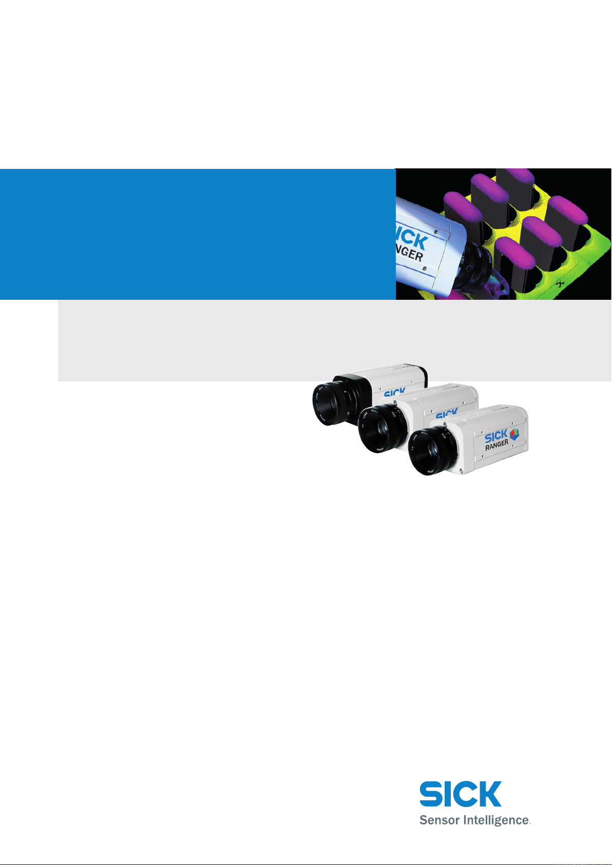
Ranger E/D

MultiScan 3D camera with Gigabit Ethernet (E)

3D camera with Gigabit Ethernet (D)

Please read the complete manual before attempting to operate your Ranger.

WARNING

Turn off power before connecting

Never connect any signals while the Ranger unit is powered.

Never connect a powered Ranger E/D Power-I/O terminal or powered I/O signals to a Ranger.

Do not open the Ranger

The Ranger unit should not be opened. The Ranger contains no user serviceable parts inside.

Safety hints if used with laser equipment

Ranger is often supposed to be used in combination with laser products.

The user is responsible to comply with all laser safety requirements according to the laser safety standards IEC 60825 – 1 and 21 CFR 1040.10/11 (CDRH) respectively.

Please read the chapter Laser Safety in Appendix B carefully.

Turn off the laser power before maintenance

If the Ranger is used with a laser (accessory), the power to the laser must be turned off before any maintenance is performed. Failure to turn this power off when maintaining the unit may result in hazardous radiation exposure.

ISM Radio Frequency Classification - EN55011 - Group1, Class A

Class A equipment is intended for use in an industrial environment. There may be potential difficulties in ensuring electromagnetic compatibility in other environments, due to conducted as well as radiated disturbances.

Explanations:

Group1 – ISM equipment (ISM = Industrial, Scientific and Medical)

Group 1 contains all ISM equipment in which there is intentionally generated and/or used conductively coupled radio-frequency energy which is necessary for the internal functioning of the equipment itself.

Class A equipment is equipment suitable for use in all establishments other than domestic and those directly connected to a low voltage power supply network which supplies buildings used for domestic purposes.

Class A equipment shall meet class A limits.

Note: Although class A limits have been derived for industrial and commercial establishments, administrations may allow, with whatever additional measures are necessary, the installation and use of class A ISM equipment in a domestic establishment or in an establishment connected directly to domestic electricity power supplies.

Please read and follow ALL Warning statements throughout this manual.

Windows and Visual Studio are registered trademarks of Microsoft Corporation.

All other mentioned trademarks or registered trademarks are the trademarks or registered trademarks of their respective owner.

SICK uses standard IP technology for its products, e.g. IO Link, industrial PCs. The focus here is on providing availability of products and services. SICK always assumes that the integrity and confidentiality of data and rights involved in the use of the above-mentioned products are ensured by customers themselves. In all cases, the appropriate security measures, e.g. network separation, firewalls, antivirus protection, patch management, etc., are always implemented by customers themselves, according to the situation.

Subject to change without prior notice.

Reference Manual

Contents

Ranger E/D

Contents

1 Introduction ...................................................................................................................................6

2 Overview......................................................................................................................................... 8

2.1 Measuring with the Ranger..................................................................................................... 8

2.2 Mounting the Ranger............................................................................................................... 9

2.3 Configuring the Ranger..........................................................................................................10

2.3.1 Ranger Studio ..........................................................................................................10

2.3.2 Measurement Methods ...........................................................................................11

2.4 Developing Applications........................................................................................................17

2.5 Triggering ...............................................................................................................................18

3 Mounting Rangers and Lightings...............................................................................................19

3.1 Range (3D) Measurement..................................................................................................... 20

3.1.1 Occlusion..................................................................................................................21

3.1.2 Height Range and Resolution..................................................................................21

3.1.3 Main Geometries......................................................................................................22

3.2 Intensity and Scatter Measurements ...................................................................................23

3.3 MultiScan ............................................................................................................................... 23

3.4 Color Measurements ............................................................................................................. 24

3.5 Light sources for Color and Gray Measurements ................................................................25

3.5.1 Incandescent lamps.................................................................................................25

3.5.2 Halogen lamps .........................................................................................................25

3.5.3 Fluorescent tubes ....................................................................................................26

3.5.4 White LEDs ............................................................................................................... 26

3.5.5 Colored LEDs............................................................................................................ 27

4 Ranger Studio..............................................................................................................................28

4.1 Ranger Studio Main Window.................................................................................................28

4.1.1 Visualization Tabs .................................................................................................... 29

4.2 Zoom Windows ......................................................................................................................31

4.3 Parameter Editor ...................................................................................................................32

4.3.1 Flash retrieve and store of parameters .................................................................. 33

4.4 Using Ranger Studio..............................................................................................................33

4.4.1 Connect and Get an Image......................................................................................33

4.4.2 Adjust Exposure Time ..............................................................................................35

4.4.3 Set Region-of-Interest .............................................................................................. 35

4.4.4 Collection of 3D Data............................................................................................... 36

4.4.5 Getting a Complete Object in One Image................................................................37

4.4.6 White Balancing the Color Data ..............................................................................37

4.4.7 Visualizing Color Images.......................................................................................... 39

4.4.8 Save Visualization Windows....................................................................................39

4.4.9 Save and Load Measurement Data ........................................................................ 40

5 Configuring Ranger E and D .......................................................................................................41

5.1 Selecting Configurations and Components.......................................................................... 41

5.2 Setting Region-of-Interest......................................................................................................42

5.3 Different Triggering Concepts ...............................................................................................43

5.4 Enable Triggering...................................................................................................................43

5.5 Pulse Triggering Using an Encoder ....................................................................................... 45

5.5.1 Triggering Scans.......................................................................................................45

5.5.2 Embedding Mark Data............................................................................................. 46

Reference Manual

Contents

Ranger E/D

5.6 Setting Exposure Time...........................................................................................................47

5.7 Range Measurement Settings ..............................................................................................49

5.8 Details on 3D Profiling Algorithms........................................................................................ 50

5.9 Color Data Acquisition...........................................................................................................54

5.9.1 White Balancing ....................................................................................................... 54

5.9.2 Color Channel Registration......................................................................................55

5.10 Calibration.............................................................................................................................. 56

5.10.1 Calibrated Data ........................................................................................................ 57

5.10.2 Rectified Images ...................................................................................................... 57

5.10.3 Physical Setup..........................................................................................................58

5.10.4 Calibration and 3D Cameras................................................................................... 59

6 Ranger D Parameters .................................................................................................................61

6.1 System settings .....................................................................................................................61

6.2 Ethernet Settings................................................................................................................... 61

6.3 Image Configuration .............................................................................................................. 62

6.4 Measurement Configuration ................................................................................................. 63

7 Ranger E Parameters..................................................................................................................67

7.1 System settings .....................................................................................................................67

7.2 Ethernet Settings................................................................................................................... 67

7.3 Image Configuration .............................................................................................................. 68

7.4 Measurement Configuration ................................................................................................. 70

7.5 Measurement Components ..................................................................................................72

7.5.1 Horizontal Threshold (HorThr) ................................................................................. 72

7.5.2 Horizontal Max (HorMax).........................................................................................76

7.5.3 Horizontal Max and Threshold (HorMaxThr) ........................................................... 77

7.5.4 High-resolution 3D (Hi3D)........................................................................................79

7.5.5 High-resolution 3D (Hi3D COG) ............................................................................... 80

7.5.6 Gray ..........................................................................................................................83

7.5.7 HiRes Gray................................................................................................................ 84

7.5.8 Scatter ......................................................................................................................85

7.5.9 Color and HiRes color ..............................................................................................86

8 iCon API .......................................................................................................................................89

8.1 Connecting to an Ethernet Camera ......................................................................................90

8.2 Retrieving Measurement Data.............................................................................................. 92

8.2.1 IconBuffers, Scans, Profiles and Data Format ....................................................... 92

8.2.2 Accessing the Measurement Data..........................................................................93

8.2.3 Polling and Call-back ...............................................................................................95

8.2.4 Handling Buffers ...................................................................................................... 95

8.2.5 Mark Data.................................................................................................................96

8.3 Changing Camera Configuration........................................................................................... 97

8.3.1 Using Parameter Files..............................................................................................97

8.3.2 Setting Single Parameter Values.............................................................................97

8.4 Error Handling........................................................................................................................ 98

8.5 Calibration and Post Processing of Buffers..........................................................................99

8.5.1 Filter Classes............................................................................................................ 99

8.5.2 Extraction Filter ......................................................................................................100

8.5.3 Calibration Filter.....................................................................................................100

8.5.4 Rectification Filter..................................................................................................101

8.5.5 Color Registration filter..........................................................................................101

8.5.6 Color Generation Filter...........................................................................................103

Reference Manual

Contents

Ranger E/D

9 Hardware Description .............................................................................................................. 105

9.1 Sensor ..................................................................................................................................105

9.1.1 Light Sensitivity ......................................................................................................105

9.1.2 Color Filter Layout ..................................................................................................106

9.1.3 High-resolution Rows .............................................................................................107

9.1.4 Color response .......................................................................................................107

9.1.5 Standard and high-resolution color differences...................................................109

9.2 Electrical Connections.........................................................................................................110

9.3 Technical Data.....................................................................................................................112

9.4 Dimensional Drawing ..........................................................................................................114

Appendix............................................................................................................................................ 115

A Ranger E and D Models.......................................................................................................115

B Laser Safety.........................................................................................................................116

C Recommended Network Card Settings ..............................................................................117

D Recommended Switches.....................................................................................................118

E iCon Device Configuration...................................................................................................118

F Connecting Encoders...........................................................................................................119

G Ranger E/D Power-I/O terminal..........................................................................................121

H Laser Safety Key Box (ICT-B)...............................................................................................123

Chapter 1 Reference Manual

Ranger E/D

Introduction

1 Introduction

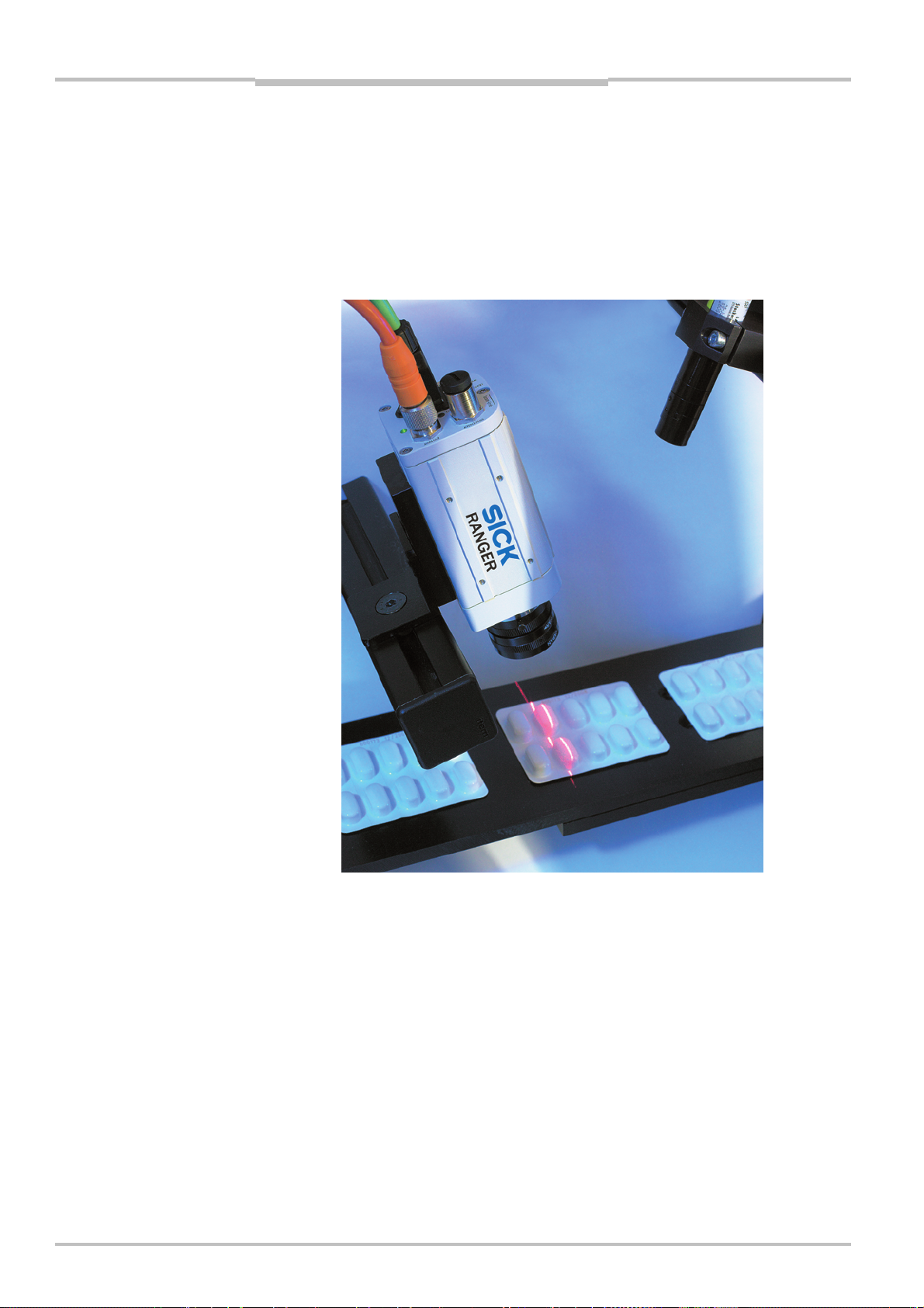
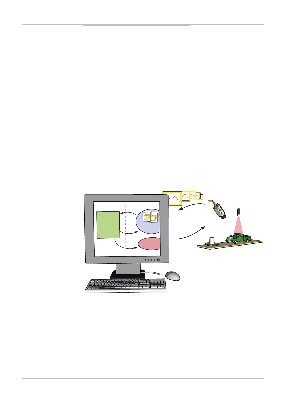
The Ranger is a high-speed 3D camera intended to be the vision component in a machine vision system. The Ranger makes measurements on the objects that passes in front of the camera, and sends the measurement results to a PC for further processing. The measurements can be started and stopped from the PC, and triggered by encoders and photoelectric switches in the vision system.

Figure 1.1 – The Ranger as the vision component in a machine vision system.

The main function of the Ranger is to measure 3D shape of objects. Depending on model and configuration, the Ranger can measure up to 35 000 profiles per second.

In addition to measure 3D – or range – the Ranger can also measure color, intensity and scatter:

Range measures the 3D shape of the object by the use of laser triangulation. This can

be used for example for generating 3D images of the object, for size rejection or volume measurement, or for finding shape defects.

Intensity measures the amount of light that is reflected by the object. This can for

example be used for identifying text on objects or detecting defects on the objects’ surface.

Color measures the red, green, and blue wavelength content of the light that is

reflected by the object. This can be used to verify the color of objects or to get increased contrast for more robust defect detection.

Scatter measures how the incoming light is distributed beneath the object’s surface.

This is for example useful for finding the fiber direction in wood or detecting delamination defects.

Reference Manual Chapter 1

Ranger E/D

Introduction

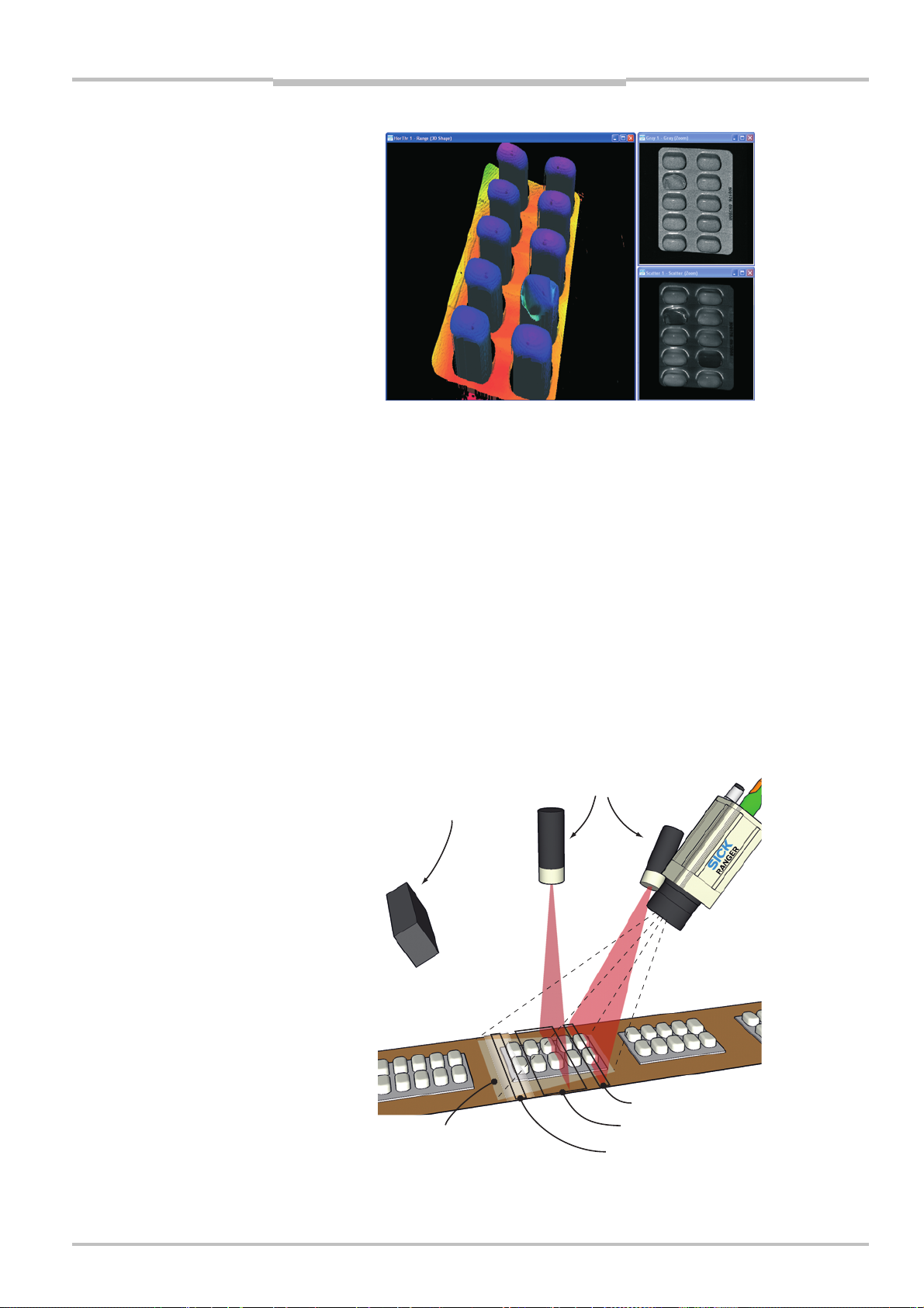
Figure 1.2 – 3D (left), intensity (top right), and scatter (bottom right) images of a blister

pack with one damaged blister and two empty blisters.

There are four different models of the Ranger available:

Ranger C Connects to the PC via CameraLink.

Ranger E Connects to the PC through a Gigabit Ethernet network.

ColorRanger E Combines the function of a Ranger E camera and a three-color line scan

camera.

Ranger D A low-cost, mid-performance version of the Ranger E, suitable for meas-

uring 3D only in applications without high-speed requirements. The Ranger D can measure up to 1000 profiles per second.

The Ranger C, E and ColorRanger E models are MultiScan cameras, which mean that they can make several types of measurements on the object in parallel. This is achieved by applying different measurement methods to different parts of the sensor.

By selecting appropriate illuminations for the different areas of the measurement scene, the Ranger can be used for measuring several features of the objects at the very same time.

Lasers

White light

Scatte

Field-of-vie

Figure 1.3 – Measuring several properties of the objects at once with MultiScan, using

multiple light sources.

3D measurement

Grayscale

Chapter 2 Reference Manual

Ranger E/D

Overview

2 Overview

2.1 Measuring with the Ranger

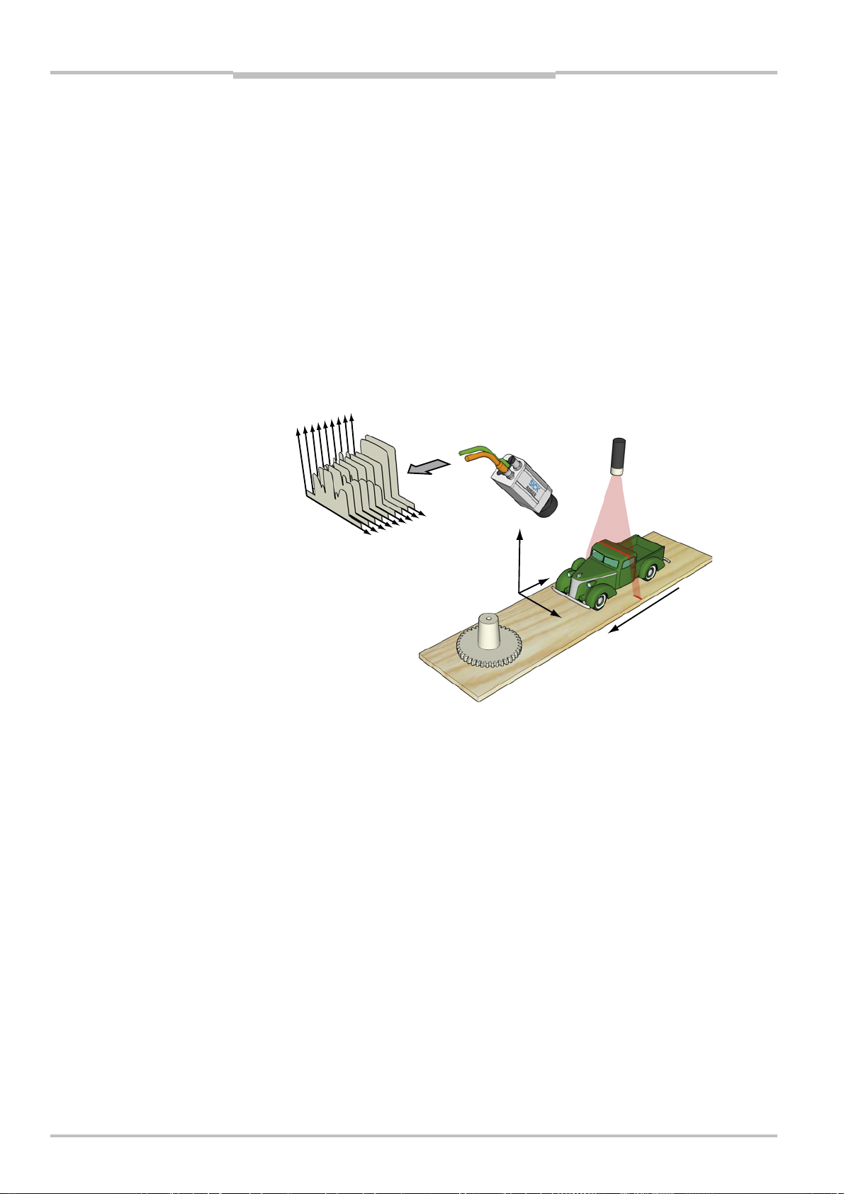
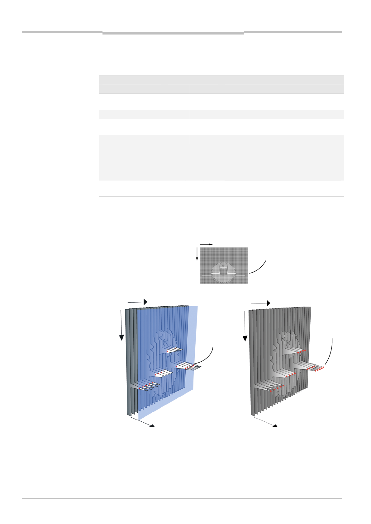
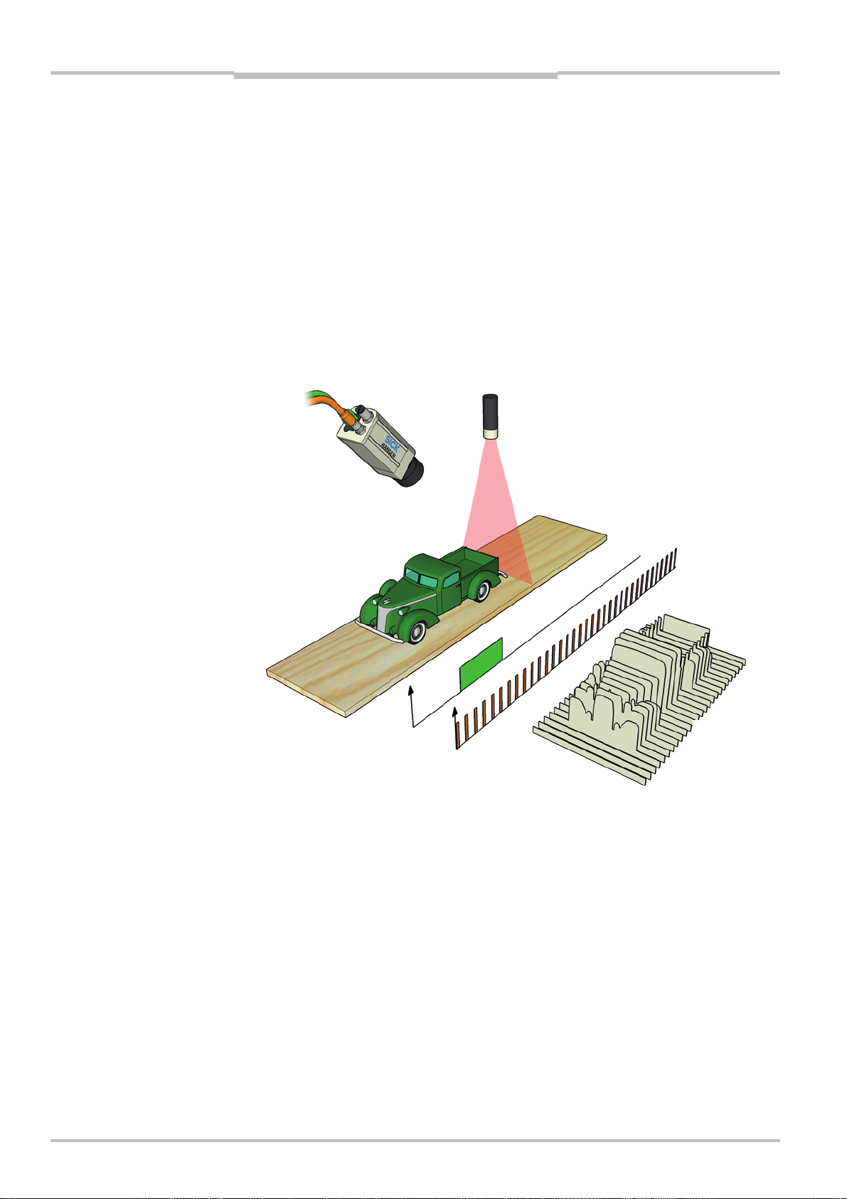
Each time the Ranger makes a measurement, it measures along a cross-section of the object in front of it. The result of a measurement is a profile, containing one value for each measured point along the cross-section – for example the height of the object along its width.

For the Ranger to measure an entire object, the object (or the Ranger and illumination) must be moved so that the Ranger can make a series of measurements along the object. The result of such a measurement is a collection of profiles, where each profile contains the measurement of a cross-section at a certain location along the transportation direction.

Profiles

Figure 2.1 – Measuring the range of a cross-section of an object.

For some types of measurements, the Ranger will produce more than one profile when measuring one cross-section. For example, certain types of range measurements will result in one range profile and one intensity profile, where the intensity profile contains the reflected intensity at each measured point.

In addition, the Ranger C, Ranger E and ColorRanger E models – being MultiScan cameras –can also make parallel measurements on the object. This could for example be used for measuring surface properties of the objects at the same time as the shape. If the Ranger is configured for MulitScan measurements, the Ranger may produce a number of profiles each time it makes one measurement – including multiple profiles from one cross-section of the object, as well as profiles from parallel cross-sections.

In this manual, the term scan is used for the collection of measurements made by the Ranger at one point in time.

Note that the range measurement values from the Ranger are not calibrated by default – that is:

 Range values (z coordinates) are given as row – or pixel – locations on the sensor.  The location of a point along the cross-section (x coordinate) is given as a number

representing the column on the sensor in which the point was measured.

 The location of a point along the transport direction (y coordinate) is represented by for

example the sequence number of the measurement, or the encoder value for when the scan was made.

(range)

(width)

Transportation

Reference Manual Chapter 2

Ranger E/D

Overview

To get calibrated measurements – for example coordinates and heights in millimeters – you need to transform the sensor coordinates (row, column, profile id) into world coordinates (x, y, z). This transformation depends on a number of factors, for example the distance between the Ranger and the object, the angle between the Ranger and the laser, and properties of the lens. You can do the transformation yourself, or you can use the 3D Camera Coordinator – a tool that performs the transformation from sensor coordinates (row, column) to world coordinates (x, z). The world coordinate in the movement direction (y) is obtained by the use of an encoder. For more information about the Coordinator tool, see the 3D Camera Coordinator Reference Manual.

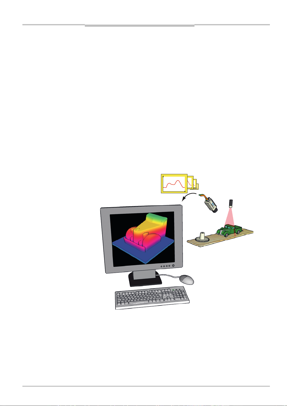
In a machine vision system, the Ranger acts as a data streamer. It is connected to a PC through either a CameraLink connection (Ranger C) or a Gigabit Ethernet network (Ranger D & E). The Ranger sends the profiles to the computer, and the computer runs a custom application that retrieves the profiles and processes the measurement data in them. This application can for example analyze the data to find defects in the objects and control a lever that pushes faulty objects to the side.

Before the Ranger can be used in a machine vision system, the following needs to be done:

 Find the right way to mount the Ranger and light sources.  Configure the Ranger to make the proper measurements.  Write the application that retrieves and processes the profiles sent from the Ranger.

The application is developed in for example Microsoft Visual Studio, using the APIs that are installed with the Ranger development software.

Figure 2.2 – Profiles are sent from the Ranger to a PC, where they are analyzed by a

custom application.

2.2 Mounting the Ranger

Selecting the right way of illuminating the objects to measure, and finding the right way in which to mount the Ranger and lightings are usually critical factors for building a vision system that is efficient and robust.

Chapter 2 Reference Manual

Ranger E/D

Overview

The Ranger must be able to capture images with good quality of the objects in order to make proper measurements. Good quality in vision applications usually means that there is a high contrast between the features that are interesting and those that are not, and that the exposure of the images does not vary too much over time.

A basic recommendation is therefore to always eliminate ambient light – for example by using a cover – and instead use illumination specifically selected for the measurements to be made.

The geometries of the set-up – that is the placement of the Ranger, the lightings and the objects in relation to each other – are also important for the quality of the measurement result. The angles between the Ranger and the lights will affect the type and amount of light that is measured, and the resolution in range measurements.

Chapter 3 'Mounting Rangers and Lightings' contains an introduction to factors to consider when mounting the Ranger and lightings.

2.3 Configuring the Ranger

Before the Ranger can be used in a machine vision application, the Ranger has to be configured to make the proper measurements, and to deliver the profiles with sufficient quality and speed. This is usually done by setting up the camera in a production-like environment and evaluating different ways of mounting, measurement methods and parameter settings until the result is satisfactory.

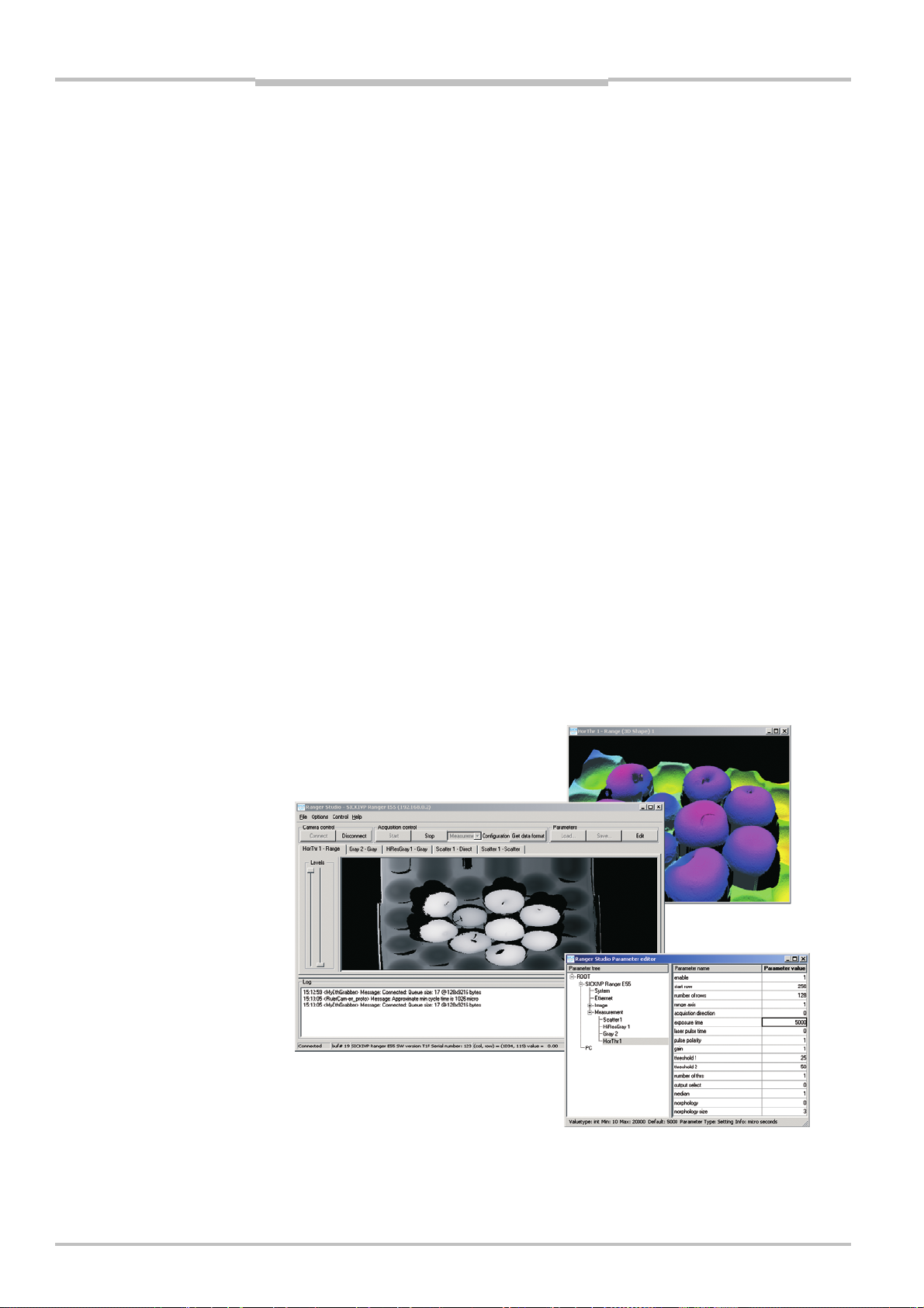
2.3.1 Ranger Studio

The Ranger Studio application – which is a part of the Ranger development software – can be used for evaluating different set-ups of the camera, and for visualizing the measurements. With Ranger Studio, you can change the settings for the camera and instantly see how the changes affect the measurement result.

Once the Ranger has been set up to deliver measurement data that meets the requirements, the settings can be saved in a parameter file from the Ranger Studio. This parameter file is later used when connecting to the Ranger from the machine vision application.

Figure 2.3 – Configuring the Ranger with Ranger Studio.

Reference Manual Chapter 2

Ranger E/D

Overview

2.3.2 Measurement Methods

One part of configuring the Ranger is selecting which measurement method to use for measuring. The Ranger has a number of built-in measurement methods – or components – to choose from.

Which component to use is of course depending on what to measure – range, intensity, color, or scatter – but also on the following factors:

 Required speed and resolution of the measurements  Characteristics of the objects to measure  Conditions in the environment

The MultiScan feature of the Ranger C, Ranger E and ColorRanger E models means that different components can be applied on different areas of the sensor. These components will then be measuring simultaneously.

For each component there are a number of settings – parameters – that can be used for fine-tuning the quality and performance of the measurements. These parameters specify for example exposure time and which part of the sensor to use (Region-of-interest, ROI).

Range Components

The Range components are used for making 3D measurement of objects.

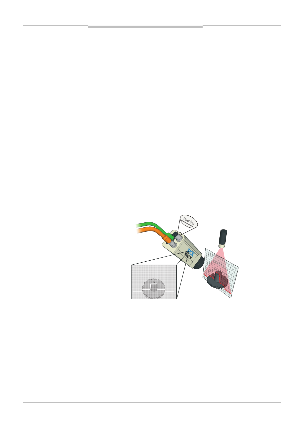
The Ranger uses laser triangulation when measuring range, which means that the object is illuminated with a laser line from one direction, and the Ranger is viewing the object from another direction. The laser line shows up as a cross-section of the object on Ranger’s sensor, and the Ranger determines the height of each point of the cross-section by locating the vertical location of the laser line.

The Ranger and the laser line should be oriented so that the laser line is parallel to the rows on the Ranger’s sensor. The Ranger E and D have a laser line indicator on the back plate, indicating in which direction it expects the laser line to be oriented.

Sensor image

FIgure 2.4 – Laser triangulation.

Laser line indicator

(Ranger E and D only)

Laser line

Chapter 2 Reference Manual

Ranger E/D

Overview

The Ranger E and ColorRanger E models have five different components for measuring range, the Ranger C has three components, and the Ranger D has one component. They differ in which method is used for locating the laser line:

Range component Model

E C D

Horizontal threshold X X Fast method, using one or two intensity

thresholds.

Horizontal max X X Uses the maximum intensity.

Horizontal max and threshold

High-resolution 3D (Hi3D)

High-resolution 3D (Hi3D COG)

For each measured point, the Ranger returns a range value that represents the number of rows – or vertical pixels – from the bottom or top of the ROI to where it detected the laser line.

X Uses one intensity threshold.

X X Measures with higher resolution, using an

algorithm similar to calculating the centerof-gravity of the intensity.

The algorithm used by the Hi3D component differs between Ranger E and Ranger D, as does the format of the output.

X X Measures with higher resolution, using a

true center-of-gravity algorithm.

Rows

Columns

Rows

Columns

ensor image

Threshold

Rows

Projected

laser line

Columns

Intensity

Threshold Ma

Figure 2.5 – Different methods for determining the range by analyzing the light intensity

in each column of the sensor image: Threshold determines the range by locating intensities above a certain level, while Max locates the maximum intensity in each column.

Intensity

Reference Manual Chapter 2

Overview

Ranger E/D

If the Ranger was unable to locate the laser line for a point – for example due to insufficient exposure, that the laser line was hidden from view, or that the laser line appeared outside of the ROI – the Ranger will return the value 0. This is usually referred to as miss- ing data.

In addition to the range values, the Horizontal max, Horizontal threshold and max, and Hi3D for Ranger E/C and ColorRanger E also deliver intensity values for the measured points along the laser line. The intensity values are the maximum intensity in each column of the sensor, which – in the normal case – is the intensity of the reflected laser line.

(1)

The resolution in the measurements depends on which component that is used. For example the Horizontal max and threshold method returns the location of the laser line

with ½ pixel resolution, while the Hi3D method has a resolution of

/16th of a pixel.

Note that the Ranger delivers the measured range values as integer values, which represent the number of “sub-pixels” from the bottom or top of the ROI. For example, if the Ranger is configured to measure with ½ pixel resolution, a measured range of 14,5 pixels is delivered from the Ranger as the integer value 29.

Besides the measurement method, the resolution in the measurements depends on how the Ranger and the laser are mounted, as well as the distance to the object. For more information on how the resolution is affected by how the Ranger is mounted, see chapter 3 'Mounting Rangers and Lightings'.

The performance of the Ranger – that is, the maximum number of profiles it can deliver each second – depends on the chosen measurement method, but also on the height of the ROI in which to search for the profile. The more rows in the ROI, the longer it takes to search.

Therefore, one way of increasing the performance of the Ranger is to use a smaller ROI.

Figure 2.6 – A ROI with few rows will be faster to analyze than a ROI with many rows.

Note that the maximum usable profile rate can be limited by the characteristics of the object’s surface and conditions in the environment.

(1)

The intensity value from Ranger C’s Hi3D component is the accumulated intensity in

each column, which in the normal case still can be used as a measurement of the intensity of the reflected laser line.

Chapter 2 Reference Manual

Ranger E/D

Overview

Intensity Components

The Intensity components are used for measuring light reflected from the object. They can be used for example for measuring gloss, inspecting the structure of the object surface, or inspecting print properties. They can also be used for measuring how objects respond to light of different wavelengths, by using for example colored or IR lightings.

There are two different intensity components:

Gray Measures reflected light along one or several rows on the sensor.

HiRes Gray Available in Ranger models C55 and E55. Uses a special row on the

sensor that contains twice as many pixels as the rest of the sensor (3072 pixels versus 1536 pixels). The profiles delivered by the HiRes Gray component therefore have twice the resolution compared with the ordinary Gray component.

Figure 2.7 – Grayscale (left) and gloss (right) images of a CD. Both the text and the crack

are present in both images, but the text is easier to detect in the left image while the crack is easier to detect in the right.

Some of the range components also deliver intensity measurements. The difference between using these components and using the Gray or HiRes Gray component is that the Gray and HiRes Gray components measure the intensity on the same rows for every column on the sensor, whereas the range components measure the intensity along the triangulation laser line, which may be located on different sensor rows for each column.

Reference Manual Chapter 2

Ranger E/D

Overview

Color Components

The Color components are used for measuring the red, green and blue wavelength content of the light reflected from the object. They can be used for inspecting color properties, for example to detect discolorations or to sort colored objects.

The Color components are only available on the ColorRanger models, which are equipped with a sensor where some of the rows are coated with a red, green, or blue filter. The filter layout is described in 9 “Hardware Description”.

There are two different color components:

Color Measures reflected light along three color filtered rows on the sensor.

HiRes Color Available in the ColorRanger E55. Uses special rows on the sensor that

contains twice as many pixels as the rest of the sensor (3072 pixels versus 1536 pixels). The profiles delivered by the HiRes Color component therefore have twice the resolution compared with the ordinary Color component.

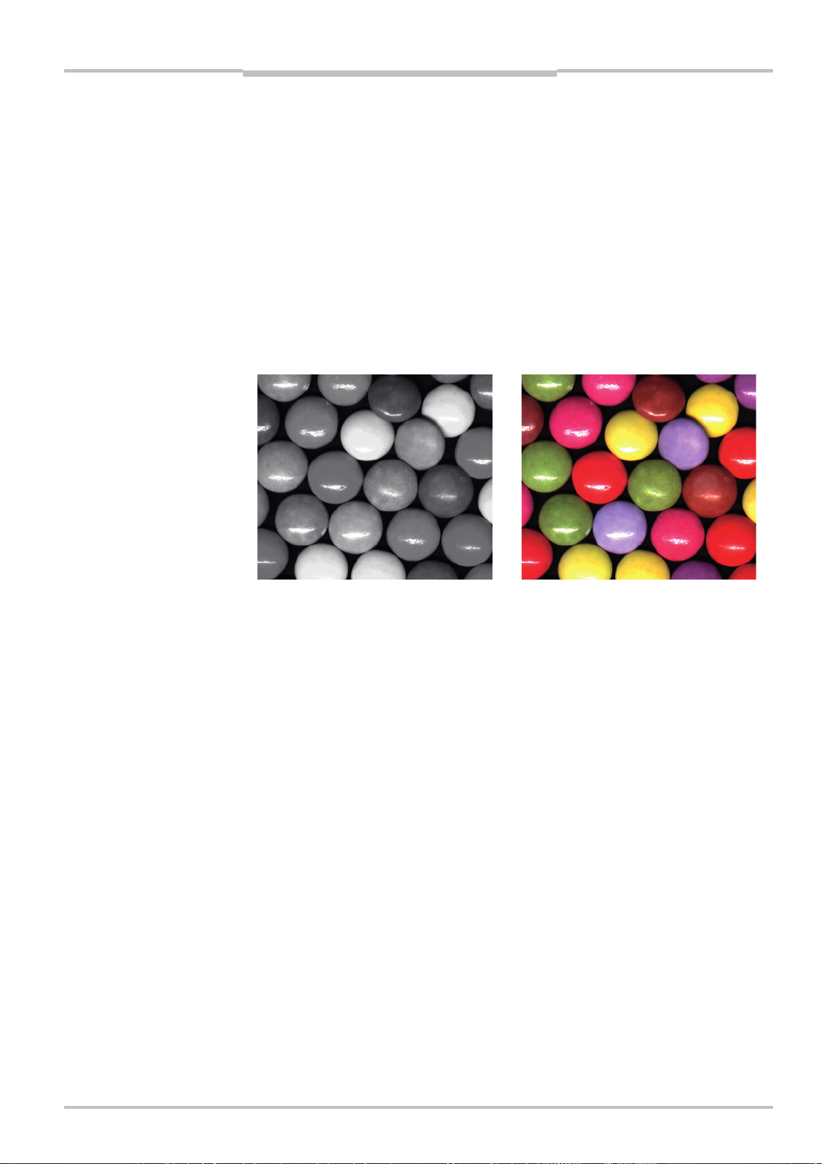
Figure 2.8 – Grayscale (left) and color (right) images of candy. The color image makes it

possible to differentiate between the colors, for example for counting or sorting.

The Color components make measurements in three different regions on the sensor simultaneously. The data is delivered as separate color channels – one channel for each sensor area. The color channels can then be merged into high quality color images on the PC by using the APIs in the Ranger development software.

Chapter 2 Reference Manual

Ranger E/D

Overview

Scatter Component

The Scatter component is used for measuring how the light is distributed just below the surface of the object. This can be used for emphasizing properties that can be hard to detect in ordinary grayscale images, and is useful for example for detecting knots in wood, finding delamination defects, or detecting what is just below a semi-transparent surface.

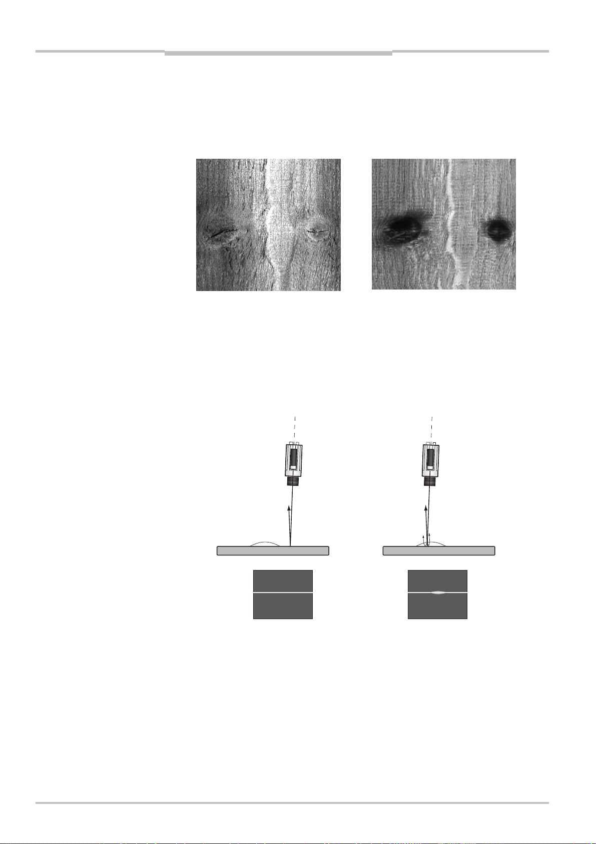
Figure 2.9 – Grayscale (left) and scatter (right) images of wood. The two knots are easy to

detect in the scatter image.

The scatter component measures the intensity along two rows on the sensor, and the result is two intensity profiles – one that should be the center of the laser line (direct), and one row a number of rows away from the first row (scatter).

The scatter profile can be used as it is as a measurement on the distribution of the light, but the result will usually be better if the scatter profile is normalized with the direct intensity profile.

Ranger

Laser

Bubble

Figure 2.10 –Using scatter to detect delamination defects. Where there are no defects,

very little light is reflected below the surface, resulting in a sharp reflex and low scatter response. Where there is a defect, the light is scattered in the gap between the layers, resulting in a wider reflection and thus high scatter response.

Reference Manual Chapter 2

Overview

Ranger E/D

2.4 Developing Applications

Once the Ranger has been configured to deliver the measurement data of the right type and quality, you need to write an application that takes care of and uses the data. This application is developed in for example Visual Studio, using one of the APIs that are delivered with the Ranger.

There are two APIs included with the development software for Ranger: iCon C++ for use with C++ in Visual Studio 2005/2008/2010, and iCon C for use with C. Both APIs contain the same functions but differ in the syntax.

The APIs handle all of the communication with the Ranger, and contain functions for:

 Starting and stopping the Ranger  Retrieving profiles from the Ranger  Changing Ranger configuration

Most of these functions are encapsulated in two classes:

Camera Used for controlling the Ranger.

FrameGrabber Collects the measurement data from the Ranger.

Your application establishes contact with the Ranger camera by creating a Camera object. It then creates a FrameGrabber object to set up the PC for collecting the measurement data sent from the Ranger. When your application needs measurement data, it retrieves it from the FrameGrabber object.

(2)

Application

iCon API

Profiles

Buffers

Frame

Grabber

Control

Request

Camera

Control

Figure 2.11 – All communication with the Ranger is handled by the API.

When the Ranger is measuring, it will send a profile to the PC as soon as it has finished measuring a cross-section. The FrameGrabber object collects the profiles and puts them in buffers – buffers that your application then retrieves from the FrameGrabber. Your application can specify the number of profiles in each buffer, and it is possible to set it to 1 in order to receive one profile at a time. However, this will also add overhead to the application and put extra load on the CPU.

(2)

For Ranger C, this requires that the Ranger is connected to a frame grabber board that

is supported by the Ranger APIs. If a different frame grabber is used, the measurement data is retrieved using the APIs for that frame grabber.

Chapter 2 Reference Manual

Ranger E/D

Overview

2.5 Triggering

There are two different ways in which external signals can be used for triggering the Ranger to make measurements:

Enable Triggers the Ranger to start making a series of scans. When the

Enable signal goes high, the Ranger will start measuring a specified number of scans. If the signal is low after that, the Ranger will pause and wait for the Enable signal to go high again; otherwise it will continue making another series of scans.

The Enable signal could for example come from a photoelectric switch

located along the conveyor belt. It is also useful for synchronizing two or more Rangers.

Pulse triggering Triggers the Ranger to make one scan. This signal could for example

come from an encoder on the conveyor belt. The Ranger C can also be triggered by the CC1 signal on the CameraLink interface.

Enable

Pulse

triggering

Figure 2.12 – Triggering the Ranger with Enable and Pulse triggering signals.

If pulse triggering is not used, the Ranger will measure in free-running mode – that is, make measurements with a regular time interval determined by the Ranger’s cycle time. The actual distance on the object between two profiles is then determined by the speed of the object – that is, how far the object has moved during that time.

When measuring the true shape of an object, you should always use an encoder with the Ranger. With the signals from the encoder as pulse triggering signals, it is guaranteed that the distance that the object has moved between two profiles is well known.

You can find the actual distance between two profiles even if the Ranger is measuring in free-running mode, as long as you have an encoder connected to the Ranger. The encoder information can then be embedded with the profiles sent to the PC as mark data. Your application can then use this information to calculate the distance between the profiles.

Profiles

Number of scans

(Scan height)

Reference Manual Chapter 3

Ranger E/D

Mounting Rangers and Lightings

3 Mounting Rangers and Lightings

Choosing the right way of mounting the Ranger and illuminating the objects to be measured is often crucial for the result of the measurement. Which method to use depends on a number of factors, for example:

 What is going to be measured (range, gloss, grayscale, scatter, etc.)  Characteristics of the surface of the objects (glossy, matte, transparent)  Variations in the shape of the objects (flat or varying height)  Requirements on resolution in the measurement results

Measuring with the Ranger means measuring light that is reflected by objects, and from these measurement draw conclusions of certain properties of the objects.

For a machine vision application to be efficient and robust, it is therefore important to measure the right type of light.

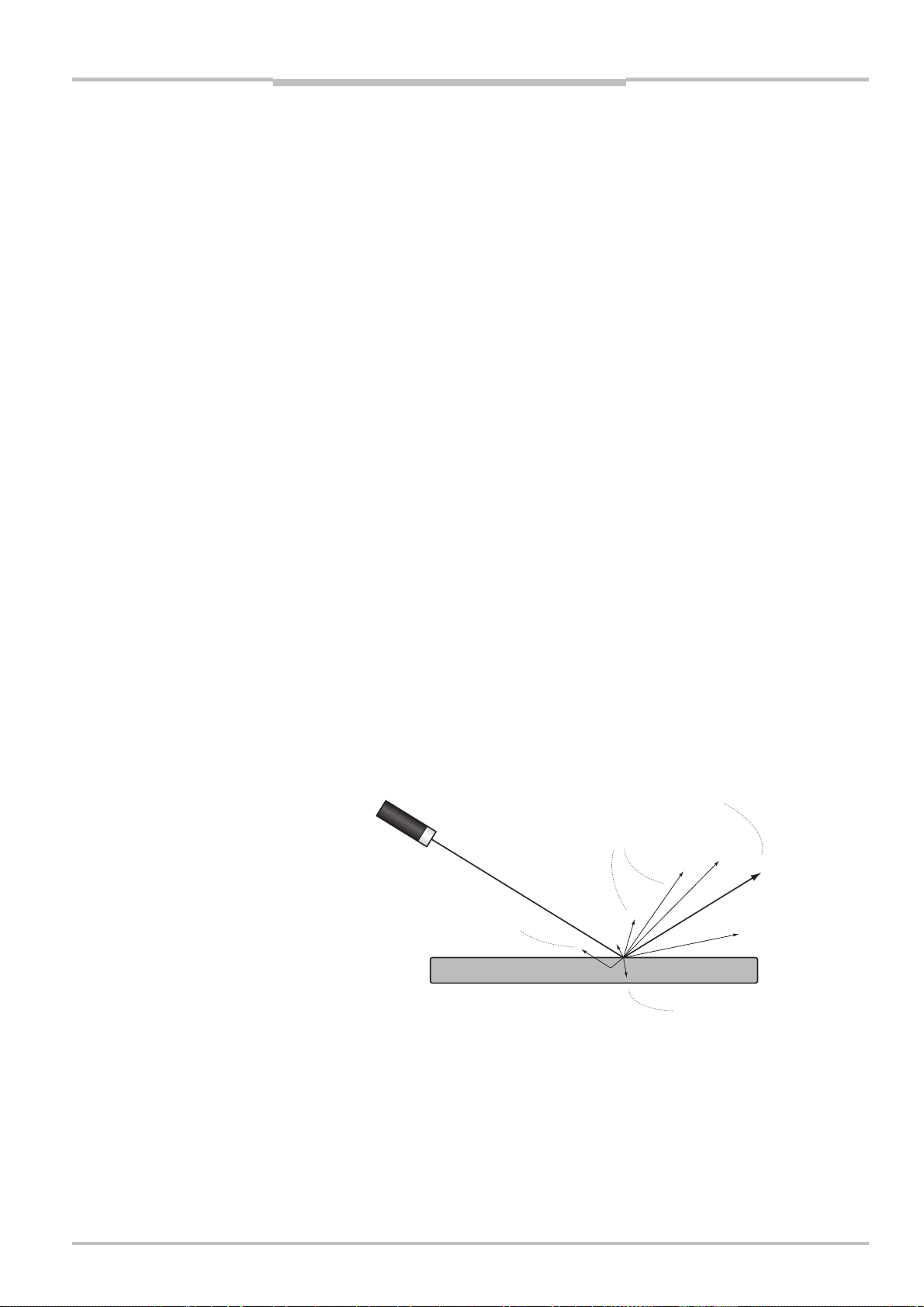
Reflections

An illuminated object reflects the light in different directions. On glossy surfaces, all light is reflected with the same angle as the incoming light, measured from the normal of the surface. This is called the specular or direct reflection.

Matte surfaces reflect the light in many different directions. Light reflected in any other direction than the specular reflection is called diffuse reflection.

Light that is not reflected is absorbed by or transmitted through the object. Objects absorb light with different wavelengths differently. This can for instance be used for measuring color or IR properties of object.

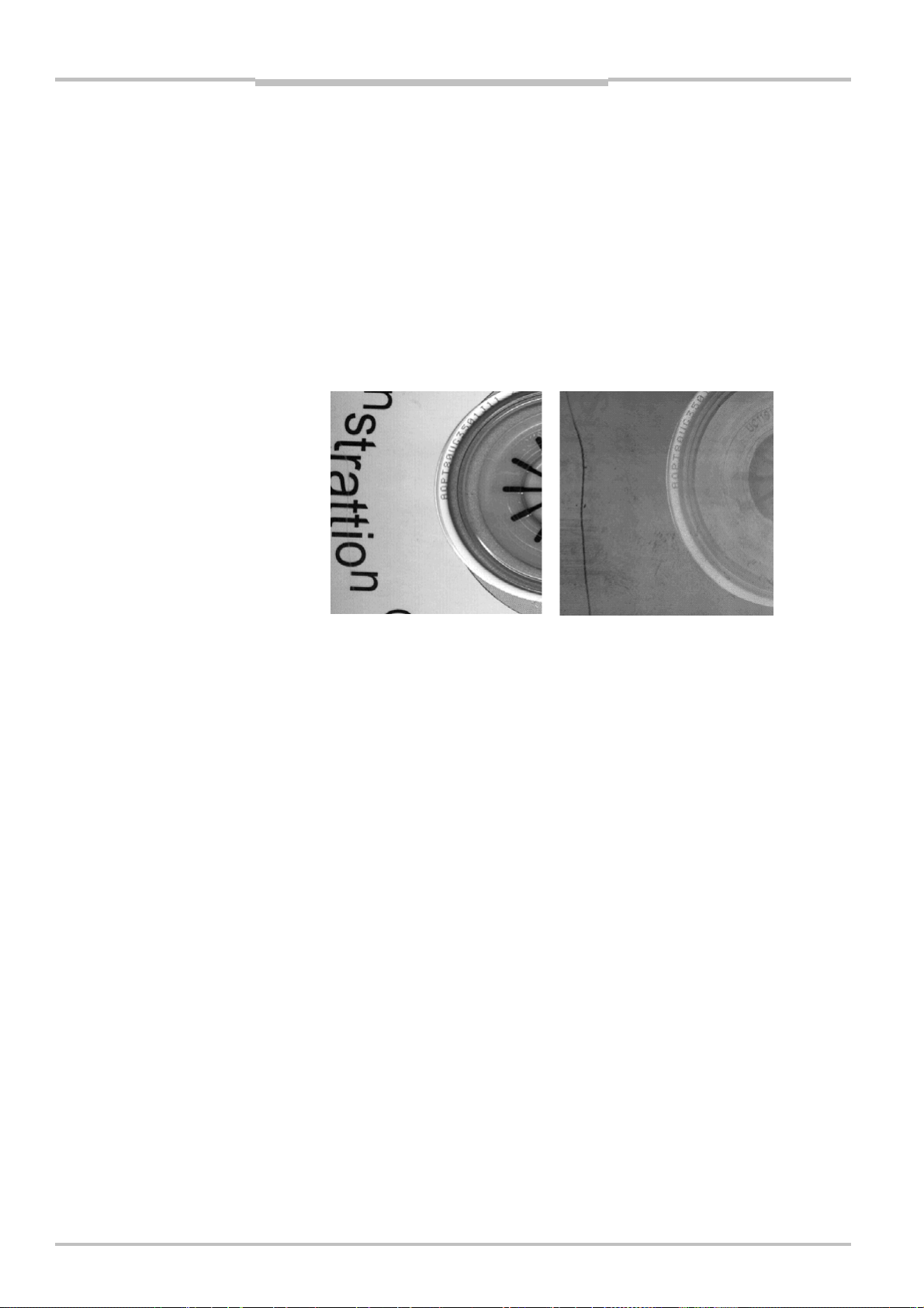
The amount of light that is absorbed usually decreases as the incoming light becomes parallel with the surface. For certain angles, almost all light will be reflected regardless of wavelength. This phenomenon is used when measuring gloss, which can be used for example for detecting surface scratches (see the example on page 26).

On some materials, the light may also penetrate the surface and travel into the object, and then emerges out of the object again some distance away from where it entered. If such a surface is illuminated for example with a laser, it appears as if the object “glows” around the laser spot. This phenomenon is used when measuring scatter. The amount and direction of the scattered light depends on the material of the object.

Specular reflection

Diffuse reflections

Scattered light

bsorbed light Transmitted light

Figure 3.1 – Direct and diffuse reflections on opaque and semi-transparent objects.

The Ranger measures one cross-section of the object at a time. The most useful illumination for this type of measurements is usually a line light, such as a line-projecting laser or a bar light.

Chapter 3 Reference Manual

Ranger E/D

Mounting Rangers and Lightings

3.1 Range (3D) Measurement

The Ranger measures range by using triangulation, which means that the object is illuminated with a line light from one direction, and the Ranger is measuring the object from another direction. The most common light source used when measuring range is a line projecting laser.

The Ranger analyzes the sensor images to locate the laser line in them. The higher up the laser line is found for a point along the x axis (the width of the object), the higher up is that point on the object.

(range)

(transport)

(width)

Figure 3.2 – Coordinate system when measuring range.

When measuring range, there are two angles that are interesting:

 The angle at which the Ranger is mounted  The angle of the incoming light (incidence)

Both angles are measured from the normal of the transport direction. The angle of the Ranger is measured to the optical axis of the Ranger – that is, the axis through the center of the lens.

Optical axis

Incidence angle

Figure 3.3 – Angles and optical axis.

The following is important to get correct measurement results:

 The laser line is aligned properly with the sensor rows in the Ranger.  The lens is focused so that the images contain a sharp laser line.  The laser is focused so that there is a sharp line on the objects, and that the laser line

covers a few rows on the sensor.

Reference Manual Chapter 3

Ranger E/D

Mounting Rangers and Lightings

3.1.1 Occlusion

Occlusion occurs when there is no laser line for the Ranger to detect in the sensor image. Occlusion will result in missing data for the affected points in the measurement result.

There are two types of occlusion:

Camera occlusion When the laser line is hidden from the camera by the object.

Laser occlusion When the laser cannot properly illuminate parts of the object.

Camera occlusion

Laser occlusion

Figure 3.4 – Different types of occlusion.

Adjusting the angles of the Ranger and the laser can reduce the effects of occlusion.

If adjusting the angle is not suitable or sufficient, occlusion can be avoided by using multiple lasers illuminating the objects from different angles (laser occlusion) or by using multiple cameras viewing the objects from different angels (camera occlusion).

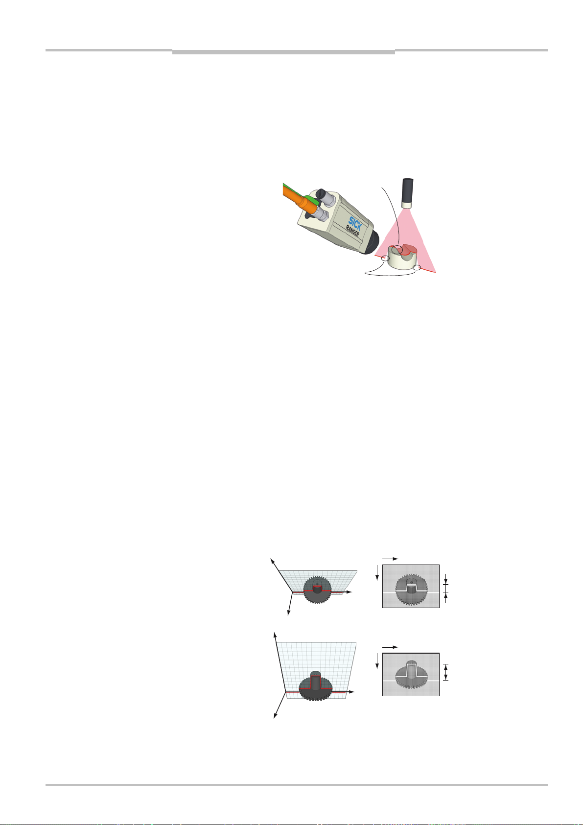
3.1.2 Height Range and Resolution

The height range of the measurement is the ratio between the highest and the lowest point that can be measured within a ROI. A large height range means that objects that vary much in height can be measured.

The resolution is the smallest height variation that can be measured. High resolution means that small variations can be measured. But a high resolution also means that the height range will be smaller, compared with using a lower resolution in the same ROI.

In general, the height range and the resolution depend on the angle between the laser and the Ranger. If the angle is very small, the location of the laser line will not vary much in the sensor images even if the object varies a lot in height. This results in a large height range, but low resolution.

On the other hand if the angle is large, even a small variation in height would be enough to move the laser line some pixels up or down in the sensor image. This results in high resolution, but small height range.

mall angle

Large angle

View from the Range

Figure 3.5 – The resolution in the measured range is higher if the angle between the laser

and the Ranger is large.

Sensor image

Measured range in pixels

Chapter 3 Reference Manual

Ranger E/D

Mounting Rangers and Lightings

3.1.3 Main Geometries

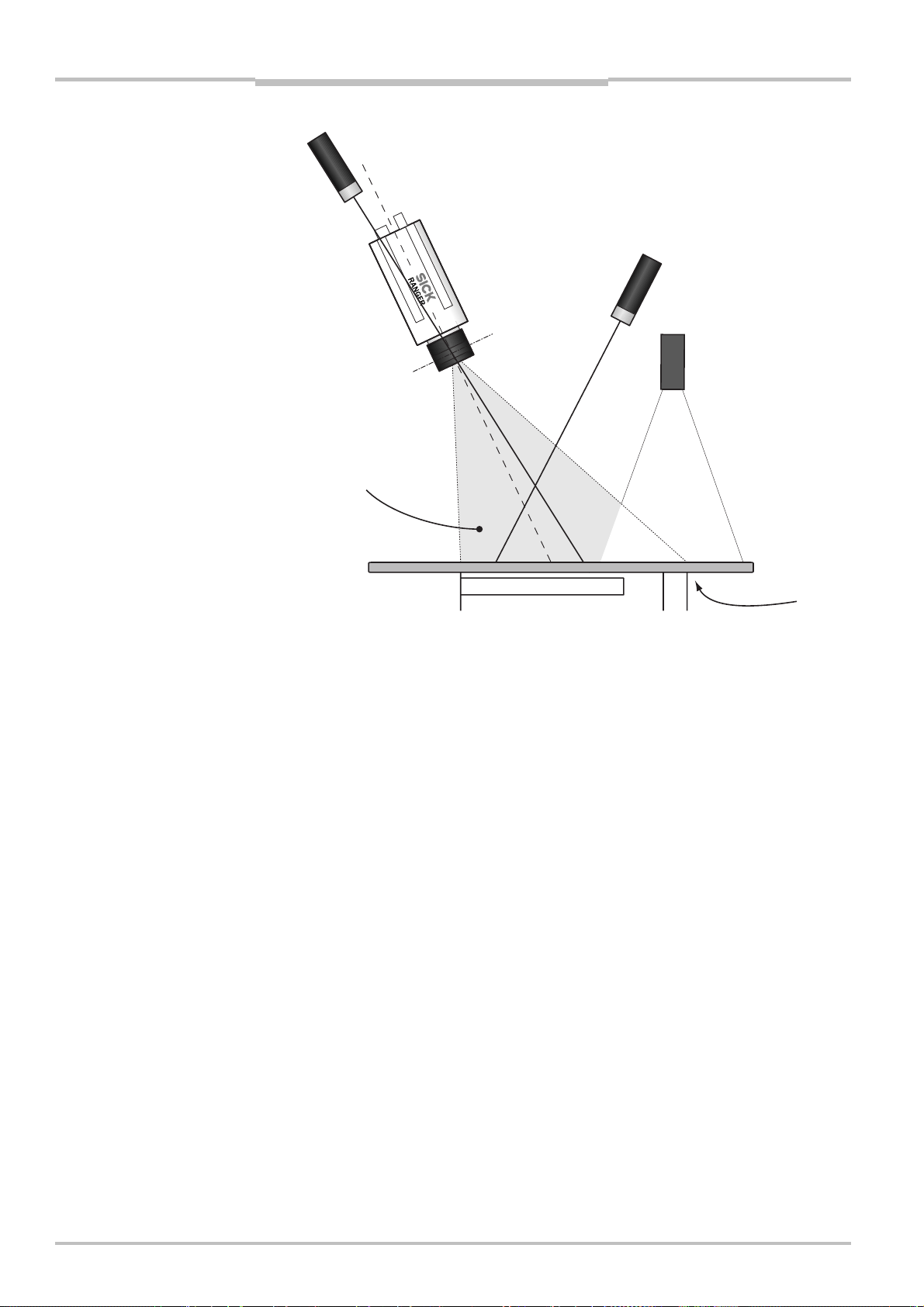
There are four main principles for mounting the camera and the laser:

Ordinary The Ranger is mounted right above the object – perpendicular to the

direction of movement – and the laser is illuminating the object from the side.

This geometry gives the highest resolution when measuring range, but

also results in miss-register – that is, a high range value in a profile corresponds to a different y coordinate than a low range value.

Reversed ordinary As the Ordinary setup, but the placement of the laser and the Ranger

has been switched so that the lighting is placed above the object.

When measuring range, the reversed ordinary geometry does not

result in miss-register, but gives slightly lower resolution than the ordinary geometry.

Specular The Ranger and the lighting are mounted on opposite sides of the

normal.

Specular geometries are useful for measuring dark or matte objects,

since it is requires less light than the other geometries.

Look-away The Ranger and the lighting are mounted on the same side of the

normal.

This geometry can be useful for avoiding unwanted reflexes but re-

quires more light than the other methods and gives lower resolution.

Ordinary Reversed ordinary

Specula

Figure 3.6 – Main geometries for mounting the Ranger and laser.

Look-away

Reference Manual Chapter 3

Ranger E/D

Mounting Rangers and Lightings

As a rule of thumb, the height resolution increases with the angle between the Ranger and the laser, but the resolution is also depending on the angle between the Ranger and the height direction (z axis).

The following formulas can be used for approximating the resolution for the different geometries, in for example mm/pixel:

Geometry Approximate range resolution

Ordinary ∆Z ≈ ∆X / tan(β)

Reversed ordinary ∆Z ≈ ∆X / sin(α)

Specular ∆Z ≈ ∆X · cos(β) / sin(α+ β)

If α = β: ∆Z ≈ ∆X / 2 · sin(α)

Look-away ∆Z ≈ ∆X · cos(β) / sin( |α–β|)

where:

∆Z = Height resolution (mm/pixel)

∆X = Width resolution (mm/pixel)

α = Angle between Ranger and vertical axis (see figure 3.6)

β = Angle between laser and vertical axis (see figure 3.6)

Note that these approximations give the resolution for whole pixels. If the measurement is made with sub-pixel resolution, the resolution in the measurement is the approximated resolution divided by the sub-pixel factor. For example, if the measurement is made with the Hi3D component that has a resolution of 1/16 ∆Z/16.

pixel, the approximate resolution is

3.2 Intensity and Scatter Measurements

For other types of measurements than range, a general recommendation is to align the light with the Ranger’s optical axis (as in figure 1.7 on page 26), or mount the lighting so that the light intersects the optical axis at the lens’ entrance pupil. By doing so, the light will always be registered by the same rows on the sensor, regardless of the height of the object, and triangulation effects can be avoided.

An exception is when gloss is going to be measured, since this type of measurement requires a specular geometry and usually a large angle. However, the triangulation effect is heavy if the objects vary in height. Therefore it is difficult – if not impossible – to measure gloss on objects that has large height variations.

3.3 MultiScan

When measuring with MultiScan, it is important to separate the light sources, so that the light used for illuminating one part of the sensor does not disturb the measurements made on other parts of the sensor.

If separating the light sources is difficult, the measurements may be improved by only measuring light with specific wavelengths, using filters and colored (or IR) lightings.

For example, an IR band pass filter can be mounted so that it covers a part of the sensor, and an IR laser can be used for illuminating the object in that part. This way, range can be measured in the IR filtered part of the sensor, and at the same time intensity can be measured in the non-filtered area using white light, without disturbing the range measurements.

For certain Ranger models, a built-in IR filter is available as an option. The IR filter is mounted so that rows with low row numbers are unaffected by the filter (0–10 for Ranger, 0–16 for ColorRanger), and rows 100–511 are filtered. Please refer to “Ranger E and D Models” on page 113 for a list of available models.

Chapter 3 Reference Manual

Ranger E/D

Mounting Rangers and Lightings

Optical axis

IR laser

scatter

Ranger with

IR option

Entrance pupil

of lens

IR laser

White light

source

Field-of-vie

Figure 3.7 – Example of MultiScan set-up using one white light source, one IR laser for

scatter measurement and one IR laser for 3D measurement, and a Ranger with the IR filter option. Note that the scatter laser is mounted so that the light beam intersects the optical axis at the lens’ entrance pupil.

IR filtered rows

0 Row: 511

512

High-resolution

row

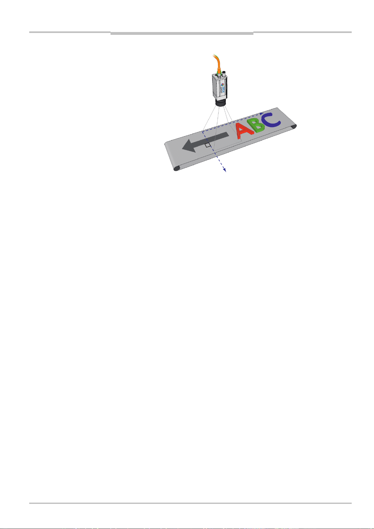
3.4 Color Measurements

The setup for color data acquisition can follow the general guidelines for Multiscan setup, with the following additions:

Geometry It is recommended to use the ordinary geometry with the camera

mounted more or less vertically above the object, since this makes the light source alignment easier.

Note that it is typically good to tilt the setup a little bit off the true vertical

alignment to avoid specular reflections.

Illumination The white light source for color acquisition needs to cover all color rows

on the sensor – that is, at least around 10 rows. It must also be ensured that the illumination covers the color region for the entire height range in the FOV.

When using the high-resolution grayscale row together with the standard

color rows, the illumination line must cover approximately 50 rows.

Alignment Since color image acquisition with ColorRanger requires that data from

different channels are registered together, it is important that the camera is well aligned with the object’ direction of movement. If this is not the case the color channel registration must also compensate for a sideway shift, which is currently not supported by the iCon API.

Reference Manual Chapter 3

Ranger E/D

Mounting Rangers and Lightings

Camera

Transportation

Camera

Figure 3.8 – Correct alignment between camera and object motion. Camera’s y-direction

should be parallel with the direction of transportation.

3.5 Light sources for Color and Gray Measurements

Different light sources have different spectral properties – that is, different composition of wavelengths. This section lists some typical light sources, some of which are commonly used for line-scan gray and color imaging applications.

A measure often used for spectral content of a light source is color temperature. A high color temperature (4-6000) indicates a “cold” bluish light and a low color temperature (2-

3000) a “warm” yellow-reddish light. Color temperature is measured in the Kelvin scale (K).

3.5.1 Incandescent lamps

Incandescent lamps are not often used in line-scan machine vision applications. This is since they commonly use low frequency AC drive current, which causes oscillations in the light.

They are warm with a typical color temperature of ~2700 K.

3.5.2 Halogen lamps

Halogen lamps are common in machine vision applications, and are often coupled to a fiber-optic extension so that shapes such as a line or ring can be generated. In the optical path a filter can be placed to alter the color temperature of the lamp.

Halogen lamps typically have a color temperature of ~3000 K, which means that the illumination has a fairly red appearance.

In a ColorRanger application using halogen illumination it is expected that the blue and green balance needs to be adjusted to be much larger than the red channel due to the strong red content. To shift the color temperature of the lamp it is also possible to insert additional filters in the light source. Filters for photography called cooling color temperature filters in the series 80A/B are recommended for this.

Chapter 3 Reference Manual

Ranger E/D

Mounting Rangers and Lightings

3.5.3 Fluorescent tubes

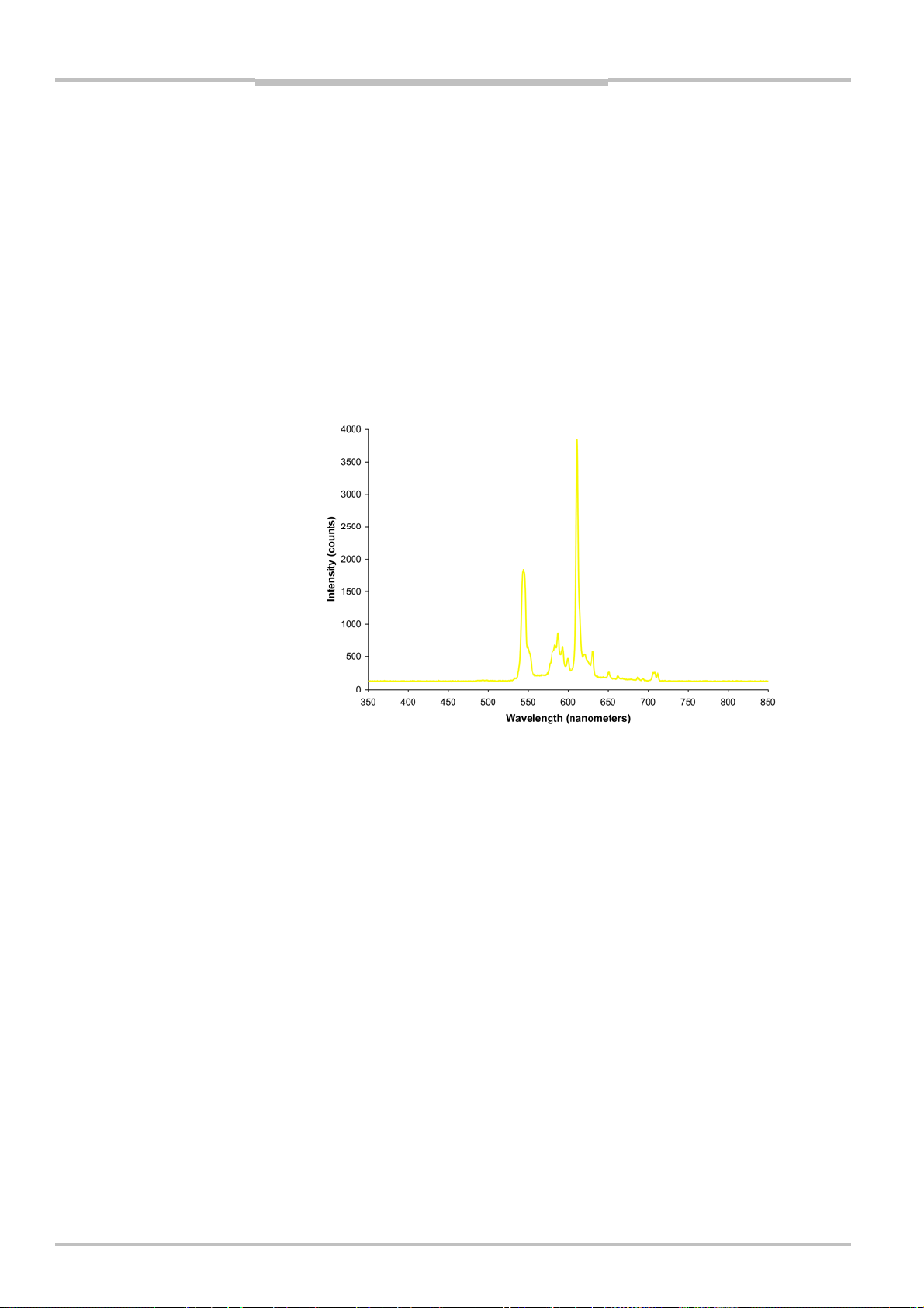
A fluorescent tube illumination has a very uneven spectral distribution, as shown in the figure below.

Furthermore, there are many different versions with different color temperature and therefore color balance. Warm white fluorescent tubes typically have color temperatures at ~2700 Kelvin, neutral white 3000 K or 3500 K, cool white 4100 and daylight white in the range of 5000 K - 6500 K.

In line-scan machine vision applications it is important that the drive frequency of the fluorescent tube is higher than the scan rate of the camera to avoid flicker in the images.

Fluorescent tubes are light efficient and have low IR content, but they are difficult to focus to a narrow line. If using IR lasers and the IR pass filter option the white illumination may cover the same region as the lasers without interference, reducing the focusing problem.

Figure 3.9 – Illustration of spectrum from “yellow” fluorescent tube illumination. [Picture

from Wikipedia.]

3.5.4 White LEDs

LEDs are commonly used in machine vision since they can be focused to different shapes and give high light power.

White LEDs have a strong blue peak from the main LED and then a wider spectrum from the phosphorescence giving the white appearance.

This type of illumination is expected to require approximately 60-70% balance on the blue and green channels compared with the red.

Reference Manual Chapter 3

Mounting Rangers and Lightings

Ranger E/D

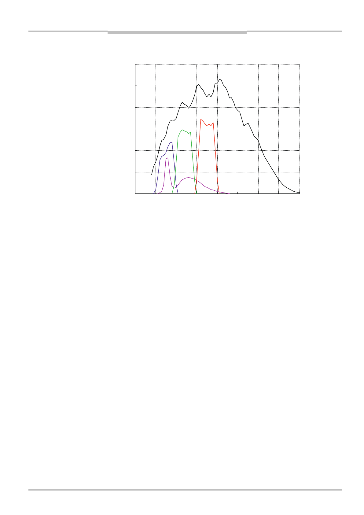
Response

[ADu per pixel / (µJ/cm

3000

2500

2000

1500

1000

500

300 400 500 600 700 800 900 1000 1100

)]

M12 Color Response

ht wavelength [nm]

Figure 3.10 –The spectrum of a white LED plotted in magenta. It has a peak in the blue

range that fits well with the blue filter on the sensor, and has a fairly low amount of red in the spectrum.

3.5.5 Colored LEDs

An LED illumination can also be made from individual red, green and blue LEDs. In this case the spectrum of each LED must fall within the respective filter bands. In this case the balance depends on the individual power of the LEDs.

Chapter 4 Reference Manual

Ranger E/D

Ranger Studio

4 Ranger Studio

Ranger Studio application is a tool for evaluating data and different set-ups of the camera. With Ranger Studio, you can change the settings for the camera and instantly see how the changes affect the measurement result from the Ranger.

Once the Ranger has been set up to deliver measurement data that meets the requirements, the settings can be saved in a parameter file.

Ranger Studio consists of a Main Window, Zoom Windows, Mouseover Information and a Parameter Editor.

Zoom Windo

Control

bar

Visualization

tab

Main window

Mouseove

Information

windo

Levels

Log

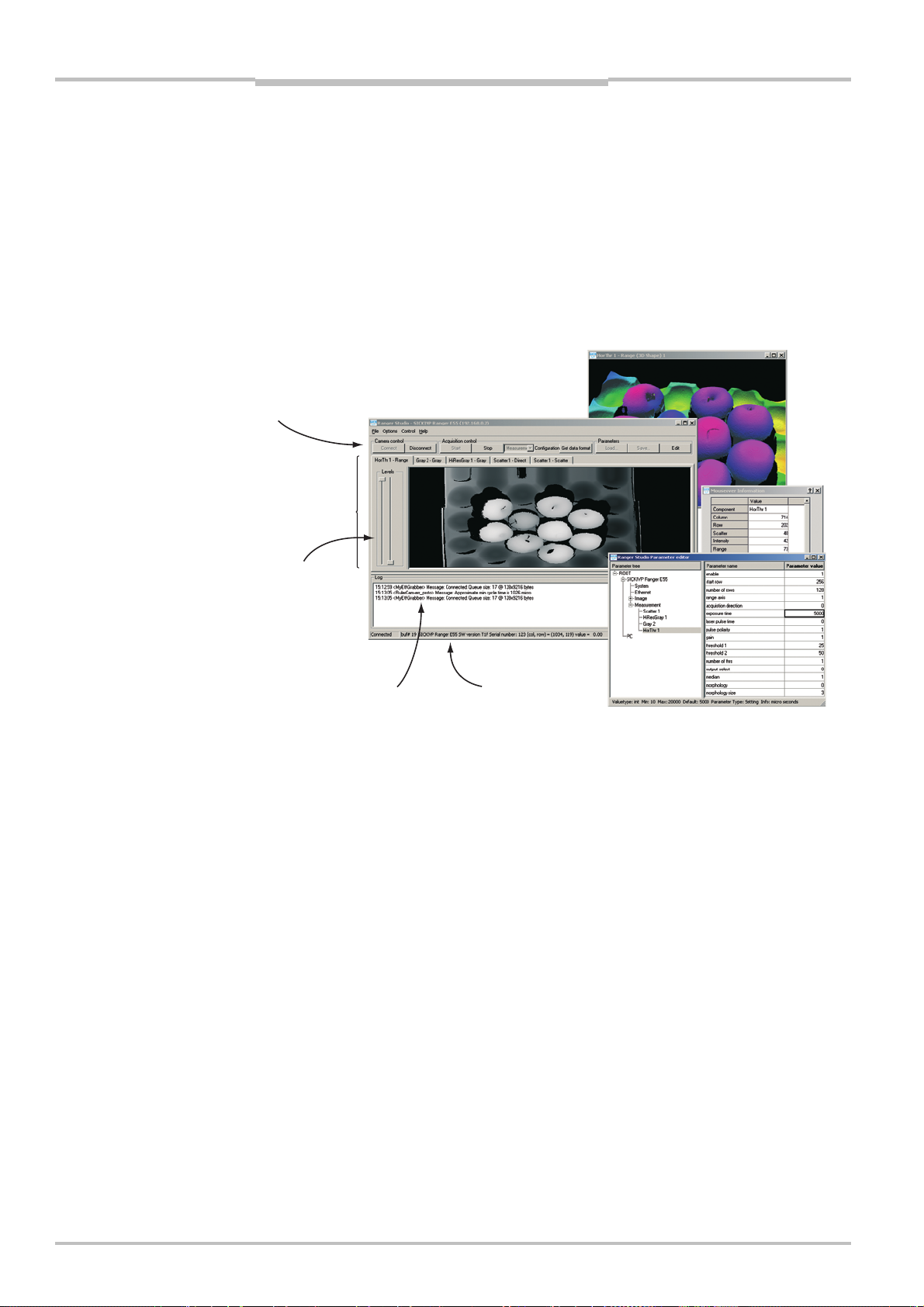
Figure 4.1 – Ranger Studio windows

Status bar

Parameter edito

4.1 Ranger Studio Main Window

The main window is the core of the application. It consists of a menu bar, a control bar with buttons, tabs with visualizations of the measurement data and levels sliders, a log area, and a status bar.

 Menu bar – menus with access to visualization windows and options.  Control bar – contains the functions for controlling the Ranger.  Visualization tabs – used for visualizing the measurements made by the camera.  Levels – used for adjusting which measurement values are visualized in the Visualiza-

tion tab.

 Log – shows error and status messages.  Status bar – shows information such as the number of scans that Ranger Studio has

received from a Ranger, and the coordinates and value for a pixel under the mouse pointer.

 Mouseover Information window – can be used for showing detailed information of the

data under the mouse pointer in a visualization tab. The window is enabled and disabled in the menu View

The buttons in the control bar are grouped into three categories:

 Camera control – contains buttons to connect and disconnect the camera.  Acquisition control – to start and stop the scanning loop and to change between meas-

uring in Image or Measurement mode. Image mode is used for set-up purposes. Measurement mode is used for collection measurement data.

 Mouseover information.

Reference Manual Chapter 4

Ranger E/D

Ranger Studio

 Parameters – to handle parameter files and to start the parameter editor.

All these tools are also available in the menus.

4.1.1 Visualization Tabs

The visualization tabs are used for visualizing the result from the camera. The main window has one tab for each type of measurement made by the Ranger with the current configuration. The visualization can be disabled and enabled by selecting Options ize. This can be useful when streaming to file, see 4.4.9 “Save and Load Measurement Data”.

The number of tabs is automatically updated as components are activated or deactivated in the configuration.

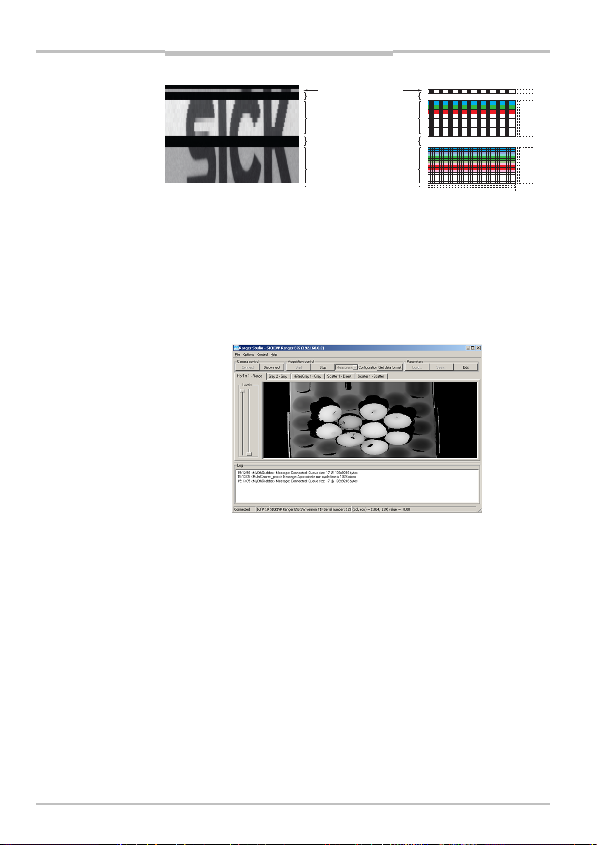
Image Mode

In Image mode (when the image configuration is active), there is one visualization tab showing a grayscale 2D image. This view can be useful for example when adjusting the exposure time, or deciding the region of interest.

 Visual-

Figure 4.2 – Visualization tab with grayscale 2D image.

The displayed image is the sensor image from the Ranger, which represents what is in the Ranger’s field of view.

For the ColorRanger E, available high-resolution rows (depending on model) can also be displayed in the image. The high-resolution rows are shown at the top of the image, above the standard rows. The display of the high-resolution rows is adopted to maintain the aspects of the sensor in the following ways:

 For ColorRanger E55, only every other column of the high-resolution rows is shown. The

high-resolution rows have twice as many columns as standard rows, but Ranger Studio displays every other column to keep the width of the image the same.

 The high-resolution rows are taller than normal sensor rows (gray 3 times, color 4

times), thereby covering a larger cross-section on the object in front of the camera. Each high-resolution row is therefore displayed in the image on 3 and 4 lines (pixels) respectively.

 The black lines in the image correspond to the area between the high-resolution rows,

and between the high-resolution rows and the standard sensor.

 Color high-resolution rows have a larger sensitivity, why the image from these rows will

appear brighter than other rows.

The high-resolution rows are displayed in image mode by enabling the Show hires parameter in the image component. Note that when displaying the high-resolution rows, the row number shown in the status bar and Info window does not match the number of the sensor row.

Chapter 4 Reference Manual

Ranger Studio

Ranger E/D

Image in Ranger Studio

Hi-Res gray row

-Res color rows

ensor layout

512

514

518

522

528

Area between rows

Standard sensor

rows

Figure 4.3 – An image showing the high resolution part and the 32 first sensor rows on

the standard sensor region. Note the black areas, brighter color highresolution part, and the reduced vertical resolution of the high-resolution rows.

Measurement Mode

When the Ranger is running in Measurement mode, the main window contains visualization tabs for each active component in the configuration. If a component produces more than one type of profiles, there is one tab for each type of profile. Each tab shows an image made from the corresponding profiles sent from the Ranger.

Figure 4.4 – Main window with tabs for range, scatter and intensity images.

The visualization tabs always shows the range measurement data as an 8-bit grayscale image. This means that the original range measurement values are translated to 255 grayscale values, where 1 (black) corresponds to the lowest range value and 255 (white) corresponds to the highest value. The value 0 means missing data.

To display the actual measured value for a point in the visualized image, place the pointer over the point in the image. The value, together with the coordinates for the point, will be displayed in the status bar and in the Info window, if open.

When measuring color, the color information for each acquired color is displayed as grayscale images in one tab each, and one tab with a compound color image. To get a proper compound color image, you have to set up the registration parameters. See “Visualizing Color Images” on page 39 for more information.

Reference Manual Chapter 4

Ranger E/D

Ranger Studio

The Levels sliders to the left in each tab can be used for visualizing only a certain range of measurement values. The right slider sets the highest value to visualize, and the left slider the lowest value. Measurement values within the range will be translated to the 255 available grayscale values, and the values outside the range will be displayed as black (1) or white (255).

This can be useful for example when studying small range variations on a part of an object that varies a lot in height. By adjusting the levels, the variations can be easier to view in the visualization image, while parts higher or lower than the selected range are ignored.

Full range of values is

visualized

Figure 4.5 – The original measurement values in a range profile (left), and corresponding

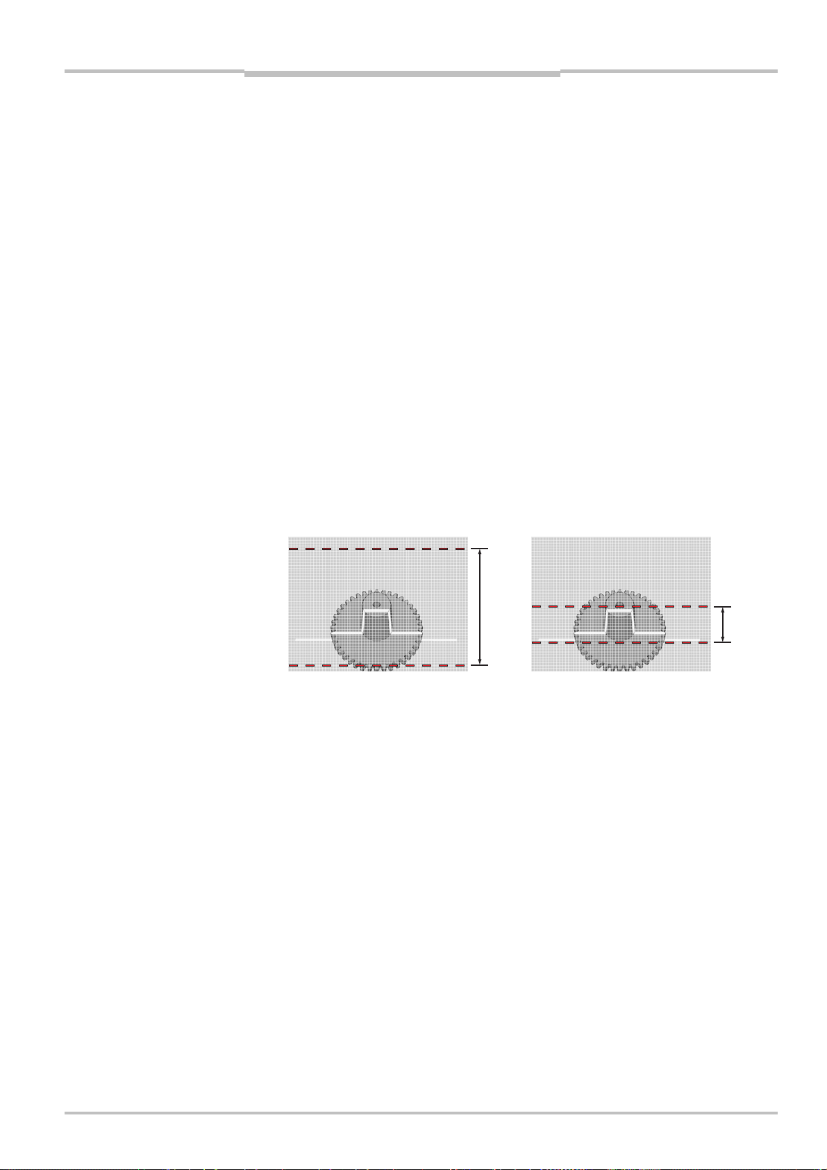
row in the image displayed in the visualization window (right), using different Levels settings.

Only selected range of

values is visualized

4.2 Zoom Windows

The zoom function is available for any visualization tab. Open a zoom window by rightclicking in the image and choosing the type of window:

 8-bit gray-scale zoom window  3D zoom window  Profile zoom window

Figure 4.6 – Range visualization tab with Profile and 3D zoom windows.

When choosing a zoom window from this menu a rectangle or a line is shown at the upper left corner of the active visualization tab, and a new zoom window is opened. Several zoom windows can be shown simultaneously.

8-bit grayscale Green rectangle. The region is displayed as a grayscale or color 2D

image.

3D zoom Yellow rectangle. The data is displayed as a 3D surface, where varia-

tion in height is also indicated by different colors. The lowest value is shown as black color.

Chapter 4 Reference Manual

Ranger E/D

Ranger Studio

Before generating the 3D surface, the data is filtered by a small

median filter to reduce noise peaks. The 3D zoom window can be of use even if the data is intensity data.

Profile zoom Blue line. The data is displayed as a profile, where range, intensity or

scatter is displayed as the y-coordinate. For color data, three profiles are displayed – one profile for red, green and blue respectively.

The contents of the zoom image are updated as the line or rectangle is moved and resized in the active visualization window:

 A rectangle is resized and moved by pressing the left mouse button pointing the cursor

on the frame or in the middle of the rectangle respectively.

 A line is moved by pressing the left mouse button while pointing the cursor on the line.

A line cannot be resized – it will always go across the entire image in the visualization tab.

When viewing the 3D zoom, you can change the perspective and coloring of the 3D surface:

 Hold down the left mouse button and move it to change the viewing direction, so that

the object can be viewed from various angles.

 Hold down the right mouse button and move it up or down in the image to remap the

coloring of the surface. This can be used to emphasize different parts of the current data.

When viewing the Profile zoom, you can zoom in on a part of the profile, by pressing the left mouse button and dragging a rectangle over the area to zoom in on. By clicking with the right mouse button in the Profile zoom window, the entire profile will be displayed in the zoom window again.

4.3 Parameter Editor

The Parameter Editor button in Ranger Studio main window opens the Parameter Editor window, which retrieves the current parameters from the system and allows you to modify parameters in the camera.

The Parameter Editor consists of three areas: Parameter tree, Parameter list and a Status bar.

Parameter tree

Parameter list

Status ba

Figure 4.7 – The Parameter editor window.

The parameter tree shows a hierarchical structure of the system configuration. When selecting an item in the parameter tree all available parameters for that item are shown in the Parameter list on the right.

Reference Manual Chapter 4

Ranger E/D

Ranger Studio

The parameter list is a table containing the parameter names and parameter values. When selecting a parameter name, or its value, information about parameter type, range etc is displayed in the status bar at the bottom. The value of a parameter can be changed in the parameter value column.

The status bar at the bottom of the parameter editor displays additional information about the selected parameter.

Value The value type of the parameter, for example int for integer.

Min The lower limit of the parameter.

Max The upper limit of the parameter.

Default The default value of the parameter.

Parameter type If the parameter is of type Argument, Setting or Property

Argument The camera needs to be stopped before changing

this parameter.

Setting This parameter can be changed at any time.

Property Read only parameter that cannot be changed.

Info Additional information about typical valid values, units, use, etc.

When you are satisfied with the parameter settings in the camera, use the button Save parameters in Ranger Studio main window to save it as a parameter file.

For detailed information about parameters, see chapters 6 “Ranger D Parameters” or

7 “Ranger E Parameters”.

4.3.1 Flash retrieve and store of parameters

Normally the parameters are reset to the factory default configuration when restarting the camera. If you want to permanently save a parameter file in the camera flash memory the following menu items can be used (in the Options->Flash parameters menu):

Store to flash Stores the currently active parameters in camera flash. Before using

the command upload the desired parameter file to the camera using

Parameters

Retrieve from flash Retrieves the parameters stored in camera flash to the active

parameters.

Auto retrieve on boot Enable the option to make the camera automatically perform the

command Retrieve from flash each time the camera boots.

 Load….

4.4 Using Ranger Studio

This section introduces the basics in Ranger Studio and describes how to:

 Get an Image from the Ranger  Adjust the Exposure time  Set the Region-of-Interest (ROI)  Collect 3D data

The common way of working is to iterate until you are satisfied with the configuration and the quality of the received data.

It is assumed that the Ranger and Ranger Studio are installed and are working properly. How to install the Ranger and Ranger Studio is described in the installation instruction. For capturing 3D images you also need movement and some kind of photoelectric switch or similar device connected to the Ranger.

We also assume that you have placed some object to measure in the laser plane. The object should fit into the field of view of the Ranger.

4.4.1 Connect and Get an Image

To get an image from the Ranger, first connect to the Ranger, and then load a suitable parameter file. Which parameter file to use depends on the model of the Ranger and

Chapter 4 Reference Manual

Ranger Studio

Ranger E/D

which measurement method you plan to use. Ranger Studio includes default parameter files for each measurement method.

In these examples, it is assumed that a pure 3D configuration is used, but it is not required.

1. Start Ranger Studio.

2. Choose Options

3. Select Options

 Type from the menu bar and select camera type.

 Show data calibrated from the menu bar if you want to see measure-

ment data in calibrated units. This option cannot be changed when connected to the camera.

4. Choose Options

 Framegrabber Options from the Ranger Studio menu bar. Check the

Fast mode checkbox if High Performance driver is installed and intended to be used. Otherwise uncheck Fast mode.

5. Click Connect on the Control bar.

6. Click Load Parameters in the Ranger Studio and select the appropriate parameter file.

7. Choose Image from Configuration.

The main window contains one visualization tab, which is still empty.

8. Click Start to start the acquisition.

The visualization tab shows the live image from the Ranger.

9. If necessary, adjust the aperture and focus of the lens to get an image that is sharp in

all areas in which to measure.

The view in the visualization tab can be used for finding an appropriate exposure time or the region-of-interest.

Reference Manual Chapter 4

Ranger E/D

Ranger Studio

4.4.2 Adjust Exposure Time

To adjust the exposure time, Ranger Studio should already be connected to the Ranger.

10. Click Parameter Editor in the Ranger Studio.

11. If needed, expand the parameter tree by clicking on the +-signs.

12. Select the Image 1 component in the parameter tree.

All parameters for this component are listed to the right.

13. Select Exposure time and change the value until the laser line is visible in the Visuali-

zation tab, but not much else of the scene is. This means that the area not hit by laser light should not be visible.

In many situations 3000 microseconds could be a good starting point, but this depends on the surface properties of the object, lens settings and light sources.

When a suitable exposure time is found and the Ranger is measuring in free-running mode, the same value should be given to two more parameters in the Parameter Editor:

14. Select the Measurement configuration in the parameter tree.

15. Select Cycle time and change the value to the same as you found as suitable expo-

sure time. The point in this example is that the cycle time should not exceed the exposure time.

16. Select the measurement component under the Measurement configuration in the

parameter tree.

17. Select Exposure time and change the value to the exposure time you found suitable

above.

Note, when measuring in free-running triggering mode the lowest value of the cycle time and the exposure time will be used as exposure time.

4.4.3 Set Region-of-Interest

The region-of-interest (ROI) is the area of the sensor image in which the Ranger will measure the object. By using a small ROI, the Ranger will normally be able to deliver profiles at a higher rate.

18. Put the highest part of the object under the laser line.

19. Click Parameter Editor in the Ranger Studio.

20. Select the Image 1 component in the parameter tree of the Parameter Editor.

21. Select Measurement ROI overlay and change the value to 1.

This will display two animated dashed lines as an overlay in the Image 1 tab. The region in between these lines is used for 3D data acquisition. Initially the lines may be at the edges of the window so you cannot see them. A good idea could be to enlarge the window.

22. Select the measurement component in the Measurement configuration in the parame-

ter tree.

23. Repeat steps 24 – 27 until the ROI is defined properly.

24. Select Start row in the parameter tree and change the value until the upper most part

of the laser line is just beneath the fist dashed line.

25. Put the lowest part of the object into the laser plane.

26. Select Number of rows and change the value until the second dashed line is just

below the lowest part of the laser line projected onto the object.

27. Click Start to start the Ranger again.

In some cases it is a good idea to not include data from the background, for example the conveyor belt.

Chapter 4 Reference Manual

Ranger E/D

Ranger Studio

4.4.4 Collection of 3D Data

When you have a suitable exposure time and the ROI have been set, the system is ready for 3D data generation. The first step is to change to measurement mode as follows:

Before starting, there should be an object under the laser line.

28. If still running, click Stop in the control bar of Ranger Studio main window.

29. Choose Measurement from Configuration.

The main window contains a number of visualization tabs, depending on the configuration.

30. Click on a Range tab.

31. Click Start in Ranger Studio.

The Visualization tab shows a grayscale image where a single profile is repeated from the top to the bottom of the window. You can view the profile in a Profile zoom window by right-clicking and choosing from the zoom menu if you like.

32. Move the object back and forth through the laser plane.

Collection of 3D profiles describing the object’s shape is displayed in the visualization tab. It may be necessary to change parameters to improve the image quality and performance.

New 3D Profiles are being collected constantly, overwriting what is displayed in the visualization window. In order to get an entire 3D image of the object, an external enable signal will come at handy. A photoelectric switch or similar device can be connected to the Ranger. Information on signal requirements and pin configuration can be found in chapter 9 “Hardware Description”.

Now, we assume a photoelectric switch or similar is connected to the Ranger.

33. Click Stop in Ranger Studio.

34. Select the Measurement configuration in the parameter tree.

35. Select the Use Enable parameter and change the value to 1.

This means that measurements will be started when the photoelectric switch is active.

36. Click Start in Ranger Studio to start the Ranger again and keep the switch active as

long as the object is in the laser plane.

37. Move the object thru the laser plane at a constant speed.

Now a 3D image (i.e. collection of 3D profiles) is displayed on the visualization tab. If the whole object does not fit into one image, try to increase the object speed.

38. If you want to save the configuration from the Ranger, click Stop to stop the acquisi-

tion.

39. Click Save parameters and give the file a name.

40. Click Disconnect.

Reference Manual Chapter 4

Ranger E/D

Ranger Studio

4.4.5 Getting a Complete Object in One Image

In many situations it is preferred to receive the measurement data for the objects in separate buffers, so that each buffer contains the measurements of one single object.

This can be achieved in several ways, for example by adjusting the speed of the conveyor belt or the profile rate from the Ranger, but also by specifying the number of scans to be collected in the buffers.

When an external enable signal is used, the Ranger will always make a number of consecutive scans after the enable signal goes high. By using for example a photoelectric switch to provide the enable signal, you can make sure that a fixed number of scans are made for each object passing the switch.

The number of scans to make is specified by the Scan height parameter, and by setting the buffer size in the frame grabber to the same value, you can assure that the measurements of one object fits into one buffer.

It is important to synchronize the frame grabber and the Ranger when using the enable signal this way, so that the first scan that the Ranger sends after the enable signal rises is placed in an empty buffer. Otherwise the measurements of the object will be split into two consecutive buffers (since the frame grabber will deliver a buffer to your application whenever it becomes full).

In this description, it is assumed that the measurement has been set up to use a photoelectric switch or similar according to the above.

41. Make a measurement and from the resulting image estimate how many scans that

would be required to fit the complete object into one image.

42. Select the Measurement configuration in the parameter tree.

43. Select ScanHeight and set it to the estimate you made. This will make the Ranger send

this amount of scans for each trig pulse (after completion of previous collection of scans).

44. Click Disconnect to synchronize the image buffers (the parameter settings of the Ranger

will remain in the Ranger unit).

45. Choose Options

46. Set the Lines per frame item to the very same value used for the ScanHeight parameter.

47. Depending on the number of lines per frame, it may also be necessary to increase the

Buffer size (that is, if a large value is used).

48. Click OK to close the window.

49. Click Connect to connect to the Ranger again.

50. Click Start to collect data and ensure that the complete object fits into one image. If

not, repeat the procedure again.

4.4.6 White Balancing the Color Data

The white balancing is necessary to ensure that proper color data is acquired. In a properly white balanced measurement, white and grey objects give equal measurement values in all three color channels, and objects appear with natural colors.

Note that no motion is needed for this process.

In this example it is assumed that the ColorRanger is configured to acquire color data, that is the configuration contains a Color component that is enabled.

 Options… from the menu bar. A Ranger Option window appears.

51. Select the Measurement configuration in the parameter tree.

52. Click Start in Ranger Studio.

53. Click on the Color tab.

54. Place a white or neutral gray object in front of the camera, so that it is visible for all

color rows.

55. Open a Profile zoom window by right-clicking and choosing from the zoom menu.

Chapter 4 Reference Manual

Ranger E/D

Ranger Studio

56. Select the Exposure time red parameter and set the exposure time for the red chan-

nel to achieve a high, non-saturated exposure for the red channel.

Overall exposure is OK, but compound image has a purple tint.

Color profiles does not match.

57. Select the Balance green parameter and adjust the value until the red and green

profiles in the Profile zoom window match.

Green and red color profiles match, but compound image still has a blue tint.

58. Select the Balance blue parameter and adjust the value until all three profiles match.

ll color profiles

match.

Compound image is neutral gray.

When adjusting the exposure times, watch the log for warning messages indicating that the efficient exposure time for any color is longer than the cycle time. If this should happen try the following:

 Increase the cycle time to allow the longer exposure time.  Decrease the exposure time of the red reference channel.  Increase the gain of one or more channels so that the exposure time can be decreased.

The shortest possible exposure time for each color channel is approximately 50 microseconds.

It is also sometimes a problem to have exposure times very close to the cycle time.

If it is difficult to achieve a proper white balancing, consider using a light source that better matches the specifications of the sensor and the color filters, as described in chapter

9 “Hardware Description”.

Reference Manual Chapter 4

Ranger E/D

Ranger Studio

4.4.7 Visualizing Color Images

To visualize images in Ranger Studio that are correctly color registered, the color registration filter used by Ranger Studio must be set up by specifying the registration parameters – that is, the distance that each color channel needs to be shifted.

Finding the Registration Parameters

The registration parameters can be determined interactively (by trial and error) or by using a program for analyzing live or recorded data.

 For trial and error, a good starting is to use the values 0, 4, 8 in one scan direction and

8, 4, 0 in the other. These values are correct if the scan speed is set so that the resolution in the scan direction (along the scanned object) is the same as the resolution in the X direction (across the scanned object).

 The development software contains an example program that can analyze live or re-

corded data and find accurate registration parameters with sub-pixel correlation. The correlation is only made in the scan direction. The program also saves the registered image to a file so that the result can be viewed.

For best result, use a black and white object with high frequency content, for example a page of text.

Configuring Registration Filter in Ranger Studio

Follow the steps below to configure the registration filter.

59. Stop the camera, if not already stopped.

60. Choose Options

61. Fill in the values for the registration parameters of the red, green and blue color

channels.

Note that one of the parameters should be set to 0, and the others must have positive values.

62. Click Start to collect data and ensure that the registration is accurate.

4.4.8 Save Visualization Windows

It is possible to save the contents of the visualization tabs – that is, the images that are displayed. The data will be saved as bitmap images in BMP format by default, but can also be saved in PNG format. Grayscale images are saved as 8-bit images, while color images are saved as 24-bit images.

Note that only the image in the current tab is saved.

63. Collect the data you want to save.

64. Stop the Ranger by clicking Stop in Range Studio.

65. Right-click in the image in a visualization tab, and choose Save image as bitmap... from

the menu that is displayed.

66. Fill in a file name in the dialog box.

This will save the image as a BMP file with the name <filename>.BMP

To save the image as a PNG file, fill in a file name that ends with .PNG in the dialog box, for example Image1.PNG

 Filter Options… from the menu bar. A Filter Options window appears.

Chapter 4 Reference Manual

Ranger Studio

Ranger E/D

4.4.9 Save and Load Measurement Data

You can save the collected measurement data, and later load and view the data in Ranger Studio, for example on another computer.

The measurement data is saved in two files: one .xml and one .dat file. The .xml file contains the format description of the collected data, and the .dat file contains the data itself. Both files must be placed in the same folder when loading the data into Ranger Studio.

To save the collected measurement data, do as follows:

67. Collect the data you want to save.

68. Choose File

69. Fill in a name for the files in the dialog box and click Save.

To load a file containing saved measurement data into Ranger Studio, do as follows:

 Save buffer... from the menu bar.

70. Make sure that Ranger Studio is disconnected from any Ranger, or that the connected

Ranger is stopped.

71. Choose File

 Load buffer... from the menu bar.

72. Select the .xml file to load in the dialog box and click Open.

Note: the corresponding .dat file must be found in the same folder as the .xml file.

You can also save a stream of measurement data – that is, all measurement data that is sent from the Ranger. In this case, the measurement data in each received buffer is saved in the same .xml/.dat format as described above.

It can be useful to disable the visualization of the data in order to lower CPU load while streaming to file. This is done by selecting Options  Visualize.

To setup streaming of measurement data do as follows:

73. Make sure that Ranger Studio is disconnected from any Ranger, or that the connected

Ranger is stopped.

74. Choose File

75. Choose a directory where the images will be streamed to.

 Stream Buffer to file... from the menu bar.

All files will be saved in the same directory on the PC, and the file name will have a sequence number added to identify to which buffer they belong. For example, if you enter the file name StreamedData when starting to save a data stream, the resulting files will be named:

StreamedData00001.xml StreamedData0001.dat

StreamedData00002.xml StreamedData0002.dat

StreamedData00003.xml StreamedData0003.dat

StreamedData00004.xml StreamedData0004.dat

...

The measurement data will be saved to files until the Ranger is stopped

Reference Manual Chapter 5

Ranger E/D

Configuring Ranger E and D

5 Configuring Ranger E and D

The Ranger E and D can be configured to fit many different applications. This enables testing of different set-ups and fine-tuning of the parameter values, in order to optimize the measurement loop and data quality.

The following can be specified when configuring the Ranger:

 Selecting configurations and components What to measure  Setting region-of-interest Where on the sensor to measure  Selecting triggering When to make a measurement  Setting exposure time For how long to expose the sensor  Component specific settings How to process the measurement result

before sending it to the PC

All this is specified by setting parameters in the Ranger. Normally, Ranger Studio is used for configuring the Ranger. The Parameter editor in Ranger Studio retrieves the current parameters from the Ranger and allows you to modify them. Configurations can be stored in a file on the PC for later use.

5.1 Selecting Configurations and Components

The Ranger can be used in two different modes:

Image The Ranger functions as a 2D camera and delivers grayscale images of

the objects.

Measurement The Ranger functions as a 3D or line scan camera, and delivers the

results from measuring cross-sections of the object.

The Image mode is normally used as a tool for evaluating different configurations of the Ranger. It is usually not suitable for use in a vision application – for example, the frame rate cannot explicitly be controlled when running in Image mode.

Parameter files containing configurations for the basic measurement set-ups are installed with the development software, and these files can be used as a starting point when configuring the Ranger for your specific application.

A parameter file contains two configurations that make it possible to use the Ranger in both Image and Measurement mode. The parameters that affect the Ranger in Image mode are contained in the Image configuration, and the parameters for the Measurement mode are contained in the Measurement configuration.

The Measurement configuration contains one or more components, which each correspond to a certain measurement type. The Image configuration contains one component. Each of the components has a number of parameters that are specific for the component, for example one parameter used for activating and deactivating the component.

When used in Image mode, the Ranger always uses the Image component. In Measurement mode, Ranger D uses the High-resolution 3D component, and for Ranger E there are up to ten different components available, depending on model. Since the Ranger E is a MultiScan camera, several measurement components can be active at the same time.

In addition to the configuration and component parameters, there are a two other groups of parameters:

Ethernet Used for specifying the communication between the Ranger and the PC

System Used for controlling lasers used with the Ranger

Chapter 5 Reference Manual

Ranger E/D

Configuring Ranger E and D

Ethernet

ystem

Image configuration

Image component

Figure 5.1 – Hierarchy of parameters for the Ranger E. Ranger D has a similar hierarchy,

but has only one measurement component.

Measurement configuration

Measurement components

5.2 Setting Region-of-Interest

The Region-of-Interest (ROI) defines what part of the sensor to use for the measurements. Using a smaller region on the sensor enables measurements at a higher rate.

The ROI is specified by two dimensions:

ROI-width Specifies which columns to use, and is set by specifying a start column

and the number of columns.

The ROI-width is set for the configuration, and is therefore common for all

components in that configuration.

ROI-height Specifies which rows to use, and is set by specifying a start row and the

number of rows.

The vertical location and height of the ROI is set for each component in a

configuration. This way, the sensor can be divided into separate regions, where each region is used for a specific type of measurement.

Note that the HiRes Gray component (on Ranger E55 models) always

uses a specific sensor row for measurement – that is, the start row is always 512 and the number of row is always 1.

Columns

Row 0

ROI-height

Row 511

ROI-width

Figure 5.2 – ROI-width and ROI-height

If two components have overlapping ROIs, the Ranger issues a warning but continues to measure. However, the measurement results will become corrupt.

Reference Manual Chapter 5

Ranger E/D

Configuring Ranger E and D

5.3 Different Triggering Concepts

Different application types require different trigger concepts. Below is a table of the most common triggering situations.

(a) Continuous flows No photoelectric switch is used.

Single scans sent continuously to the PC Examples: Crushed stone, grain, saw dust

(b) Continuous flow of

discrete objects

length

(d) Objects of variable

size

No photoelectric switch is used.

Single scans sent continuously to the PC

Resulting image buffer in PC can be analyzed as overlapping images ensuring that all objects are analyzed completely

Example: Cookies

Photoelectric switch is used.

One image per object

Examples: Bottles, automotive parts, mobile phones

Photoelectric switch is used.

Acquire scans as long as the object remains in front of the camera

Several sub-images can be stitched together in PC

Examples: Logs, fish, postal packages

(a) Continuous flow

Figure 5.3 – Trigger for different object types

(b) Continuous flow of discrete objects

(d) Objects of variable size

5.4 Enable Triggering

The Enable input is used to trigger the camera to start profile capture when the object passes a photoelectric switch. If the same photoelectric switch is connected to several cameras then synchronization at the microsecond level can be achieved.

When using the Enable input, the Scan height parameter specifies the number of scans that the Ranger should make after the Enable signal goes high. After the specified number of scans, the Ranger will either idle or continue to make another series of scans, depending on the state of the Enable signal and the setting of the Use enable parameter:

Chapter 5 Reference Manual

Configuring Ranger E and D

Ranger E/D

Use enable = 0

 The camera acquires scans continuously.

(no enable sensitivity)

Use enable = 1 (level sensitive)

 A new scan series starts each time the Enable input

has a high level as input, see figure below.

 Multiple enable flanks are ignored until all scans (scan

height parameter) have been acquired

NOTE: For the very first profile the camera requires not only a high level but also a rising flank

Use enable = 2 (rising flank sensitive)

 Camera starts scanning on positive edge on the enable

signal.

 Multiple enable trigs are ignored until all scans (scan

height parameter) have been acquired.

 When all scans (scan height parameter) have been

acquired, the camera waits for a new rising flank, see below.

Use enable = 3 (level sensitive with guaranteed end of scan in mark)

 Similar to Use enable = 1 (level sensitive), but checks

the Enable input state of the last scan in the series.

 If the Enable input was high for the very last scan, the

Ranger makes another series of scans even if the Enable is low when the new series is started.

 Suitable when using the status of the Enable signal to

detect the end of the object, for example when scanning objects of varying lengths. In this mode the PC will receive at least one profile where the status of the Enable signal is 0 in the embedded Mark data.

 This mode is only available in measurement mode

where enable information can be added with mark.

Note that it is advisable to set the Scan height parameter in the camera to the same values as the Profiles per buffer in Ranger Studio/Framegrabber API to keep the image synchronized and receive a full image after the image capture is completed

Enable interrupt.

24 V

Enable signal:

Scan acquisition

(level sensitive):

Scan acquisition

rising flank sensitive):

0 V

scan height

scan height scan height

Figure 5.4 – Timing diagram for ENABLE signal

Acquisition complete  Reading of enable signal.

scan height scan height

Reference Manual Chapter 5

Ranger E/D

Configuring Ranger E and D

5.5 Pulse Triggering Using an Encoder

5.5.1 Triggering Scans

The camera can be measuring in one of two different ways:

Pulse triggered The Ranger will make one measurement – or scan – after a specified

number of pulses have been received on the encoder inputs. This signal could for example be the differential signals Phase 1 and Phase 2 coming from an encoder on the conveyor belt.

This signal is connected to the differential inputs In1 and In2 on the

Encoder connector.

Free-running The Ranger will make measurements with a regular time interval.

In this mode, the distance between two scans may vary if the speed of

the object is not constant. To find the actual distance between two scans, you can connect an encoder to the Ranger and embed encoder data with the profiles.

In pulse triggered mode, the Ranger counts the number of pulses received on the encoder inputs using an internal counter. When the specified number of pulses has been received, a scan is triggered and the Ranger resets this counter.

To handle movements in both directions (forward and backward), the Ranger can be configured to count the pulses in different ways, resulting in different ways to trigger scans:

Mode Parameter

Position Trig mode = 3 The encoder trigs a scan for each object position.

If the object has moved backward no scans are made until the object has moved (at least) an equal distance forward.

Direction Trig mode = 4 The encoder trigs a scan when the object is moving

forward. If the object has moved backward, new scans will be made as soon as the object moves forward again.

Movement Trig mode = 5 The encoder trigs a scan when the object is moving

either backward or forward.

Pulse triggered (legacy)

Trig mode = 2 Similar to the Position mode, but is more sensitive to

vibrations (jitter).

Moving forward

Position

Direction

Movement

Figure 5.5 – Different pulse triggering modes.

Moving backward

Moving forward

again

Chapter 5 Reference Manual

Ranger E/D

Configuring Ranger E and D

The Position, Direction and Movement modes require that both encoder phases are connected to the Ranger. The pulse triggered mode can be used if only 1 of the 2 encoder phases is connected.



No encoder  Object propor-

tions are incorrect

Figure 5.6 – An encoder will keep object proportions when conveyor speed changes

The internal pulse counter will also be reset every time a measurement is started by the Enable signal, and when a parameter is changed while measuring (using the setParam- eterValue() method).

5.5.2 Embedding Mark Data

When an encoder is connected to the Ranger, it is possible to make the Ranger send encoder data – or mark data – with the profiles delivered to the PC.

This can be useful for example when measuring in free-running mode to find the actual distance between two scans if the speed of the object varies, for placing the measurement data in a timeline, or when registering color images.

The Ranger can embed two types of mark data in the profiles: Normal mark data  Either encoder value (number of encoder pulses) or se-

quence number for the scan.

 Status information such as status of Enable and Encoder

inputs when the scan was made, and number of overtrigs that may have occurred.

Extended mark data  Both encoder value and sequence number for the scan.

 Status information such as status of Enable and Encoder

inputs when the scan was made, and number of overtrigs that may have occurred.

 Time stamps for when the scan was made and for the most

recent encoder tick.

Extended mark data should be used when capturing color images, in order to get the most accurate and robust color registration.

The encoder value in the extended mark data can be set to represent different things:

Position Value reflects the position of the encoder. It is increased when the en-

coder moves forwards and decreases when it moves backwards. This allow for accurately tracking the position of an object moving both forwards and backwards.

Motion Value reflects the motion of the encoder. It increases regardless of the

encoder direction. This allows for accurately tracking the distance an object has traveled.

The time base for the clock used for the time stamps is 33 MHz. It is stored as a 32-bits integer, which gives approximately 2 minutes of counting before it wraps around.

The structure of the information in the mark data is described in section 8.2.5 “Mark Data”. The parameters used for configuring the camera to send mark data is described in section 6.4 “Measurement Configuration” for Ranger D, and 7.4 “Measurement Configu- ration” for Ranger E respectively.

Encoder  Object propor-

tions are correct

☺

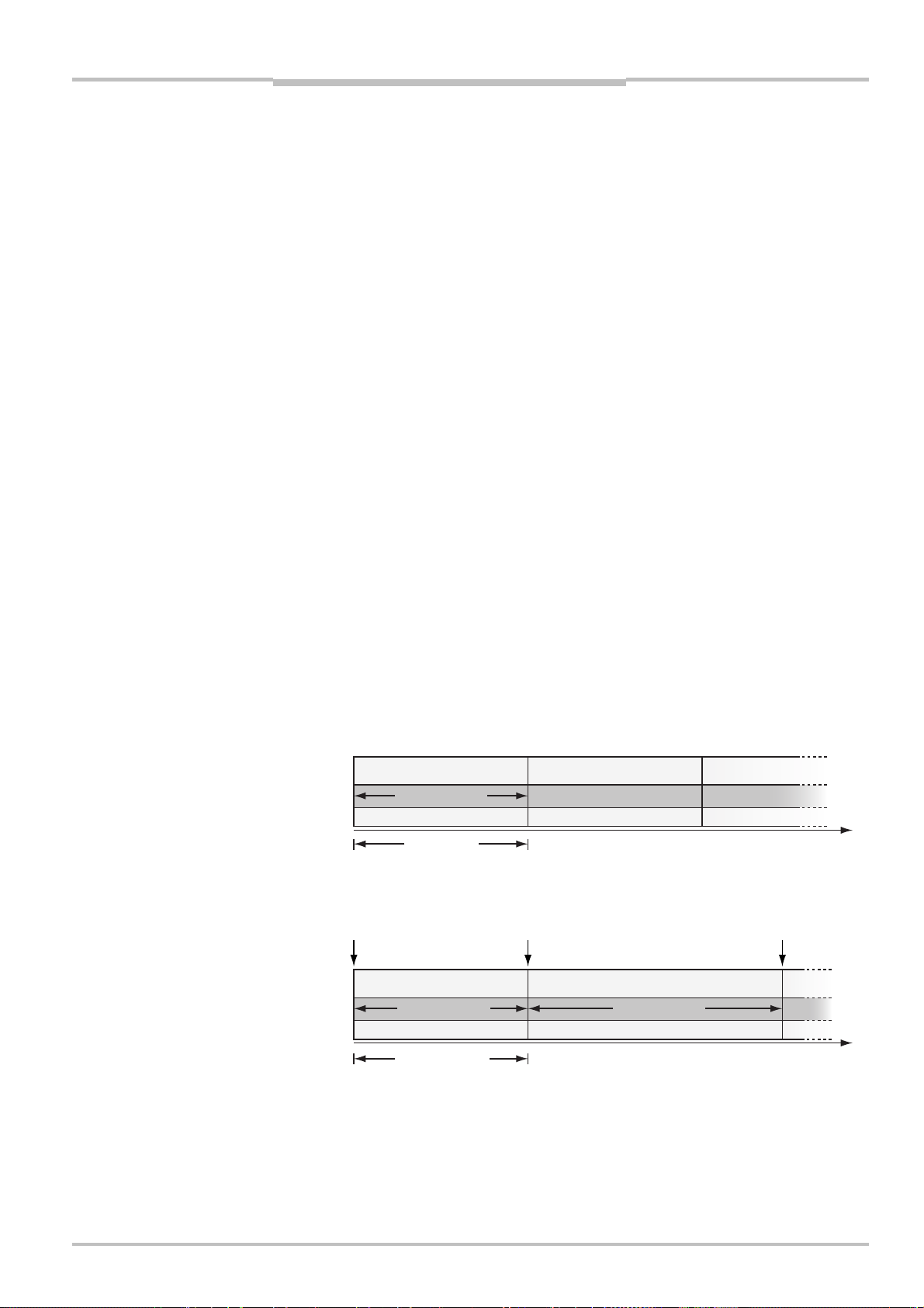
Reference Manual Chapter 5

Ranger E/D

Configuring Ranger E and D

5.6 Setting Exposure Time

Once the height of the ROI is set, there are two other settings that affect the profile rate of the Ranger:

Cycle time The time between two scans when measuring in free-running mode.

Exposure time The time during which the sensor rows in the ROI is exposed.

For natural reasons, the exposure time cannot be longer than the cycle time. If the exposure time should be set longer than the cycle time, the Ranger will expose the sensor rows during the entire cycle.

If the exposure time is instead set to be shorter than the cycle time, the sensor rows are reset at the beginning of the cycle. The exposure is then read from the sensor after the specified exposure time.

If the Ranger is measuring in free-running mode, measuring without the explicit reset will work well since the cycle time (and thus the exposure time) is constant. However, if the Ranger is measuring in pulse-triggered mode, the cycle time may vary since it now depends on the pulse triggering signal. Varying cycle times will in this case result in measurements made with different exposure times. To guarantee a constant exposure time, the exposure time should be set to be shorter than the cycle time, thereby enabling the explicit reset of the sensor rows. However, resetting the sensor takes a certain time.

Measuring with a certain exposure time and resetting the sensor rows will therefore require a longer cycle time than measuring with the same exposure time but without the reset.

The time it takes to reset the sensor rows within a ROI is equal to the shortest possible exposure time for the ROI. Both the reset time and the shortest possible exposure time depend on the height of the ROI.

Thus, when using the shortest possible exposure time, the shortest possible cycle time (and thereby the highest possible profile rate) is:

 The exposure time, when measuring without reset  Approximately two times the exposure time, when using the explicit reset

running with no explicit reset

Free

Cycle Cycle Cycle

Exposure time

Cycle time

Pulse triggering with no explicit reset

Trig Trig

Tri

Cycle Cycle

Exposure time Exposure time

Min. cycle time

Figure 5.7 – Exposure times and cycle times in different combinations of reset and trig

modes (continued on the next page).

Time

Cycle

Time

Chapter 5 Reference Manual

Configuring Ranger E and D

Ranger E/D

running with explicit reset

Free

Cycle Cycle

ed idle time

Exposure time Reset

Cycle time

Time

Pulse triggering with explicit reset

Trig

Tri

Cycle Cycle

Variable idle time

Exposure time Reset

Min. cycle time

Time

Figure 5.7 (continued)– Exposure times and cycle times in different combinations of

reset and trig modes. Note that the cycle time is longer for the same exposure time when using the explicit reset than when no reset is used.

In fact, the Ranger uses a rolling shutter sensor – that is, it reads out and resets the exposure on the sensor one row at a time. Therefore, the exposure of the first row on the sensor will start at the beginning of the cycle, while the exposure of the last row will start at the end of the reset period. The length of the exposure time for a sensor row is independent of the location of that row, since the readout is made in the same way as the resetting.

In most cases, the difference in when the exposure is started has very little effect upon the accuracy of the measurement results – much smaller than for example object properties and factors in the environment.

Sensor

Cycle time

row

Figure 5.8 - Rolling shutter.

Read-out

Reset

Exposure time

Reference Manual Chapter 5

f-g

Ranger E/D

Configuring Ranger E and D

5.7 Range Measurement Settings

The range components (HorThr, HorMax, HorThrMax and Hi3D) measure the range by determining the location of a laser line in each column of the ROI. The differences between these components are the method they use for locating the laser line in each column:

HorThr, HorThrMax The middle of the range of rows where the intensity is above a

specified threshold value.

HorMax The row where the intensity is the highest.

Hi3D Uses an algorithm similar to center-of-gravity.

Intensity

Threshold Ma

Figure 5.9 – Different methods for locating the laser line in a column. The diagrams show

the intensity for the rows in one column, which corresponds to a crosssection of the laser line.

If a column contains multiple intensity peaks (where the intensity values are above the thresholds), the HorThr and HorThrMax components will use the first encountered peak for determining the range. For these components you can specify in which direction the sensor image should be searched – from top to bottom, or from bottom to top – with the Acquisition direction parameter. This can be useful for example for avoiding reflexes to be interpreted as the laser line.

Intensity Intensity

Intensity

Row Row

Center-o

Threshold

ravity

Row

cquisition direction

Figure 5.10 –If a column contains multiple intensity peaks, the first encountered peak is

considered to be the laser line.

Note that changing the acquisition direction will also reverse the range axis – that is the range will be measured from the bottom of the ROI. You can manually reverse the axis by changing the value of the Range axis parameter.

The range component can also use pulsed illumination, in which case a signal for triggering the pulse is sent on Out2. The length of the trig pulse is set by the Laser pulse time parameter. If a configuration uses multiple range components, only one of them can pulse the illumination.

cquisition direction

Chapter 5 Reference Manual

Ranger E/D

Configuring Ranger E and D

5.8 Details on 3D Profiling Algorithms

This section contains basic information on how the measurement algorithms works and further details.

Laser Impact Position on the Sensor

The basic function of all the 3D measurements is to compute the impact position of the laser line for all columns of the selected Region-of-Interest. The light intensity distribution from the laser line along a sensor column across the laser line can be described as in the following figure.

Intensity

Sensor ro

ROI start

Figure 5.11 – The impact position of the laser in one column

The laser line will produce a distinct light peak distributed over a number of pixels along the sensor column. The center of this peak will be defined as the impact position of the laser line on that sensor column, which is the range value.

Threshold

Digitizing an analog signal by the means of a binary threshold is a common technique in signal/image-processing.

The signal in the previous figure can be thresholded by defining an intensity threshold. This operation will produce a result in which all pixels with an intensity above the threshold will be defined as logical ones. Pixels with intensity below the threshold will be defined as logical zeros. This will form a digital representation of the analog signal represented by a group of logical ones and zeros.

Intensity

ROI end

Threshold

Sensor ro

ROI start

Figure 5.12 – Digitalizing one column of the sensor image using a binary threshold

ROI end

Sensor ro

Reference Manual Chapter 5

Ranger E/D

Configuring Ranger E and D

The width of the laser light peak is defined as the number of pixels representing the peak with intensity above the threshold.

The position of the first and last pixel defining this width can be computed with a resolution of one pixel.

½-pixel position: The center of the light peak can be computed as the mid-position of the first and last pixel that represent the peak. If the width of this group consists of an even number of ones, the mid-position will fall between two pixel centers. Thus the impact position will have a resolution of half a pixel.

¼-pixel position: Two peak-widths can be computed using two different thresholds. For each width the mid-positions are computed with a resolution of half a pixel. The average of the two mid-positions is then computed giving a resolution of a quarter of a pixel.

Multiple light peaks

If several light peaks are above the threshold at the same sensor column the first peak found in the search direction is used to represent the impact position of the laser line. This may not be the correct one and will in this case result an incorrect range measurement.

Intensity

ROI start

Figure 5.13 – A too low threshold may detect multiple light peaks

In this case either the false peak must be suppressed or the threshold must be altered (as in following figure.

Intensity

False laser pea

ROI end

Threshold

Sensor row

Sensor ro

ROI start

Figure 5.14 – Altering the threshold to remove false peaks

ROI end

Sensor ro

Chapter 5 Reference Manual

Ranger E/D

Configuring Ranger E and D

In the case that the true light peak (the laser) is the first along the search order the correct range value will be computed.

Center-of-gravity

Center-of-gravity (Cog) is another method of finding the impact position of the laser line in a sensor column. With this method typical resolution of 1/16 Hi3D algorithm is based on calculations similar to Cog.

In the Center-of-gravity method a threshold is also used, but for removing background information before the AD conversion. The sensor data above the threshold is digitized to a 5–8-bit representation, and the sensor data below the threshold is set to 0 as in the ordinary thresholding. The center-of-gravity is then calculated through two sums:

of a pixel is achieved. The

(x * f (x))

Cog =

(f (x))

Where x is the sensor row and f(x) the digitized intensity level in the sensor data.

Intensity

Threshold

Sensor ro

ROI start

Intensity

ROI start

Figure 5.15 – Calculating the center-of-gravity

Median Filter

The Median filter calculates a median value on the binary data of 3-columns of the binary image (actual column and its left and right neighbors) before the range algorithm is applied. This filter pre-process the binary image data used in the profile detection of the Horizontal Threshold and Horizontal Max and Threshold components. The calculation does not increase the time for the processing.

In cases when using two thresholds this filter is applied to both binary results independently, but with the same parameters.

If both median filter and morphological is used, the morphological filter is applied before the median filter.

ROI end

Sensor ro

Morphology Filter

The morphology parameter is used for reducing noise in the sensor image before the laser line is detected. It can be used with the Horizontal Threshold and Horizontal Max and Threshold components.

Ideally the laser peak on the sensor is a smooth peak without any noise present. However, due to different noise sources the peak may be affected by noise peaks. The morphology filters are designed to reduce the effect of these noise peaks. If, when studying a Ranger

Reference Manual Chapter 5

Ranger E/D

Configuring Ranger E and D

profile, the resulting profile appears to have two distinct levels, or have profile points that appear at more or less random positions, the morphological filters can help the situation.

There are two basic binary morphology filters, shrink (erode) and expand (dilate), and both those are implemented.

Morphological filters are applied to each pixel in the image, and the result in each pixel is a function of the pixels within a defined region around that pixel. The morphological filters in Ranger work on single columns of 3-5 vertically oriented pixels, i.e. each pixel are processed together with neighbors above and below up to 2 rows away.

If the profiling algorithms use multiple thresholds each thresholded image is processed independently, but using the same filter settings.

Using the morphological filters with size 3 gives no decrease in algorithm speed, but increasing the filter size might give a small increase in minimum possible cycle time.

If both morphological and median filter is used, the morphological filter is applied before the median filter.

Figure 5.16 – Applying a morphological filter to one column of the sensor image

In a shrinking morphological filter of size Nx1 pixels the operation is defined as a Boolean AND of the pixels within the region. That is, if all pixels within the region are 1 the result is 1, otherwise 0.

Consider the binary images in the figure above. In the first noisy example, the noise peak is removed by the shrink filter, but in the second example the result is only improved by the expand filter.

In an expanding morphological filter of size Nx1 pixels the operation is defined as a Boolean OR of the pixels within the region. That is, if any pixel within the region is 1 the result is 1, otherwise 0.

Chapter 5 Reference Manual

Ranger E/D

Configuring Ranger E and D

Consider the binary images in the figure again. In the first example, the noise peak remains, and the profile result is not improved, but in the second example the result is improved.

5.9 Color Data Acquisition

The ColorRanger camera acquires color data by separately measuring the red, green and blue light reflected by the object. The color measurement results in three streams of color data, or color channels. Before the color channels can be combined into a high quality color image, they need to adjusted in terms of:

 White balancing  Color channel registration

White balancing and color channel registration can be done independent of each other and in any order. Typically, the white balancing is done when configuring the camera (so that the camera delivers white balanced color data), and the registration is done while measuring, in the PC using the iCon API.

In addition, the geometry, alignment and illumination are important when acquiring color data. See chapter 3 “Mounting Rangers and Lightings” for more guidelines on mounting the ColorRanger.

5.9.1 White Balancing

Good white balancing is necessary to ensure proper color measurements. In a properly white balanced measurement, white and grey objects give equal values in all three color channels, and objects appear with natural colors.

White balancing is necessary since different light sources have different spectral properties, combined with the fact that the sensor itself is not equally sensitive to all colors.

Figure 5.17 –Left: Poorly white balanced. The image has a violet tint, and the values for

red, green and blue channels differ. Right: Properly white balanced. The image is neutral grey and values for red, green and blue channels are almost equal.

In the color component (used for color measurements) you specify the exposure time for the red channel in microseconds. The other channels’ exposure times are specified as a percentage of the red channel’s exposure time. This way the overall brightness can be adjusted by changing only one exposure time parameter and without affecting the white balance.

Note that the exposure time for the channels cannot be longer than the cycle time. If this should happen, the camera sends a warning message indicating that the acquired data is not white balanced.

White balancing using Ranger Studio is described in section 4.4.6 “White Balancing the Color Data”.

Some light sources allow for adjustments of its spectral content. In that case it is possible to white balance by tuning the light source.

Reference Manual Chapter 5

Configuring Ranger E and D

Ranger E/D

5.9.2 Color Channel Registration

The ColorRanger makes measurements for the three color channels simultaneously, but uses different rows on the sensor. Therefore each color channel depicts different crosssections of the object in front of the camera. Each scan will acquire data from slightly different parts of the object. As the object passes in front of the camera, each position on the object is measured for red, green and blue colors at slightly different times.

When the entire object has passed the camera, it is captured in three individual images that are slightly shifted with respect to each other. The distance that the images are shifted is small, but must still be compensated for to avoid color artifacts and get high quality color images.

This compensation is known as color channel registration and basically means that the images are shifted before being combined into one color image. To do this, we need to know the distance that the images are shifted.

Red channel

Green channel

Blue channel

1t2t3

Figure 5.18 –Illustration how the 3 color rows, placed with intervals on the sensor, when

scanning an object gives an image with misregistration.

Figure 5.19 –Illustration of unregistered (left) and registered (right) color scanned by a

Ranger E camera. Note the false color edges on the letters in the unregistered image.

Registration and variations in speed

The distance to shift each color channel depends on the geometry, the profile rate, and the object speed. Should any of these vary during the measurement, the distances that the color channel images need to be shifted will also vary.

Variations in profile rate and object speed can be handled by using an encoder in the following ways:

Chapter 5 Reference Manual

Ranger E/D

Configuring Ranger E and D

 Using the encoder to trigger profiles will keep the distance between profiles constant.  Embedding encoder information (extended mark data) in the profiles will provide the

necessary information to calculate the appropriate compensation for each scan.

The distance to shift the color channels also depends on the distance between the camera and the object. Objects closer to the camera get a higher relative speed of movement over the sensor, causing the proper shift parameters to decrease, and vice versa.

To achieve the best results over the whole FOV, the registration parameters should be determined in the middle of the depth of field.

Determining Registration Parameters

The registration parameters can be found either by trial and error, or by recording and analyzing data, for example by using the example program provided with the development software.

To obtain good registration parameters, the following is recommended:

 Use a black and white object with high frequency content, for example a page of text.  When recording data, either make sure that the acquisition is triggered by an encoder,

that the acquired data contains mark data, or that the object speed is constant and the same as in the final application.

A set of registration parameters can, if encoder marking is used, work with different scan speeds but it will only work in one scan direction. If the scan direction is changed the parameters need to be inverted as described below

Registering Color Channels

The iCon API contains a color registration filter that will perform the registration of the color channels, using the registration parameters as input. Ranger Studio uses this filter to display registered, compound color images.

The color registration filter interprets the values of the registration parameters differently, depending on whether the color data contains extended mark data or not:

 If extended mark data is available in the color data, the registration parameters are

interpreted as a number of encoder ticks, and the filter can handle speed variations.

 If no mark data or normal mark data is available, the registration parameter values are

interpreted as a number of scans, and no speed variations can be handled.

Note that typically one of the color channels is the reference, and the registration parameter is 0 for this channel. The other channels should have positive parameter values that state how many scans earlier the respective sub-components should be sampled. If the scan direction is reversed the shift parameters also change so that

[0,X, Y ] -> [Y,(Y-X),0].

Since the distance between the red and blue filters is half that of the distance between the red and green the blue shift is typically twice that of the green shift, i.e. Y = 2X in the example above.

5.10 Calibration

Calibration of range data refers to the process of turning sensor coordinates (pixel positions) into real-world coordinates (e.g. mm or inches). The 3D Cameras deliver range profiles in terms of sensor positions rather than in mm or inches. By using the calibration functions of iCon you can translate sensor positions into real-world coordinates. The image below shows the relation between sensor positions and real world coordinates. Note that in this chapter, sensor positions are always denoted by a (u,v) pair where u denotes the sensor column and v is the sensor row. (u and v coordinates may be floating point numbers as the laser position is estimated on a sub-pixel level). Real world coordinates are always denoted by (x, y, z) triplets or (x, z) pairs where x is the horizontal position in the laser plane, y is the position along the direction of motion and z is the vertical position. There is also a coordinate denoted r which is the distance from the origin of the coordinate system and upwards in the laser plane. All calibration is done in the laser plane which means the result is a translation between (u, v) and (x, r). If the laser plane is perpendicular to the reference plane (XY plane) this is equal to a translation between (u, v) and (x, z) but if not you need to compensate for the skewed coordinate system. This is currently not

Reference Manual Chapter 5

Ranger E/D

Configuring Ranger E and D

handled by the calibration functions of iCon. Note that the y-axis may be directed as in either of the two cases in the image depending on if the camera is facing the approaching object or watching it from the rear.

Real-World

Object

Sensor Image

Figure 5.20 – Real-World object in laser plane and its appearance on the sensor

5.10.1 Calibrated Data

Calibrated data is a set of (x, r) points (in real-world coordinates). During the configuration of the calibration, a direct relation is established between each sensor position (u, v) and the corresponding real-world coordinate. These relations are stored in a calibration lookup table (LUT). When applying the calibration filter to a range profile, each valid (u, v) point in the profile is translated into a calibrated (x, r) point in the real world. This representation is suitable if you need to find e.g. the distance between two points in the real world or measure the height of a certain object. The image below shows an example profile as seen by the sensor (on the left) and the corresponding calibrated points in the real world coordinate system.

Sensor Image

Figure 5.21 – Sensor image and corresponding calibrated points

5.10.2 Rectified Images

Rectification of data means that a new profile is created by re-sampling the calibrated data onto a regular grid. The rectification in iCon is performed along the X-axis only. The new

Calibrated (x, r) Points

Chapter 5 Reference Manual

Ranger E/D

Configuring Ranger E and D

profile is represented in a discrete coordinate system, which is directly related to the real world coordinate system. This means that the distance in X between two adjacent values (pixels) in the profile is always the same regardless of where in the field of view they are positioned. The image below shows how a set of calibrated data points translates into a rectified profile. The final z value is represented as a floating point number to preserve the full resolution. Notice the green and yellow resulting values at the edges in the profile. You can select if you would like the rectification to return the maximum (green), minimum (yellow) or average (red) pixel height within the discrete column. Selecting the average will be better from a SNR (signal-to-noise) ratio since all the available data values are used. It will however also result in false artifacts around sharp edges as in the image. In this case it is usually a better choice to use the maximum or minimum value.

Calibrated (x, r) points Rectified profile

Figure 5.22 – Calibrated points and corresponding rectified profile

5.10.3 Physical Setup

Calibrated data can be obtained for an arbitrary physical setup. In the Ruler case, the geometry of the system is given and can only be slightly modified by tilting the Ruler. In the Ranger case, any setup can be calibrated. It is also possible to calibrate several range components belonging to the same MultiScan setup.

It is important to remember that the calibration is always made in the laser plane. This means that the obtained calibration LUT is always directly linked to the geometry of the system. In the case of reverse ordinary geometry this means that a perpendicular coordinate system is given whereas e.g. an ordinary geometry will have a skewed coordinate system. The image below shows what this means in practice.

Reference Manual Chapter 5

Ranger E/D

Configuring Ranger E and D

z, r

Reverse Ordinar

Figure 5.23 – Real-World and sensor coordinate systems for the standard geometries

As can be seen, the critical factor is the laser incident angle towards the reference plane (XY plane). If this is perpendicular (90 degrees) the x and z positions are directly given by the in-plane calibration (x, r) and the y position is given by the encoder counter. If the laser angle is not 90 degrees there will however be a dependency between r and y. There is currently no support to compensate for this in the calibration functionality of the iCon API.

Look-awa

Specular Ordinary

5.10.4 Calibration and 3D Cameras

The calibration support for 3D Cameras includes all you need to obtain calibrated and rectified range data from Ranger and Ruler cameras. All the standard range components are supported; Hi3D (DCM), Hi3D (COG), Horizontal Thresholding and Horizontal Maximum. There is currently no support for calibration of pure gray scale or scatter components but the gray and scatter subcomponents of a Hi3D component are calibrated in the same way as the Hi3D range. The calibration is built up around the concept of calibration lookuptables (LUT:s). For the Ruler, the calibration LUT is already generated in production and stored in the Ruler’s flash memory. For the Ranger a LUT needs to be generated for the selected physical setup. This divides the calibration support into two main parts; tools to generate calibration LUT:s and tools to use calibration LUT:s in your vision application software.

Tools to generate calibration LUT:s

This section only applies to Ranger cameras since Ruler cameras are shipped precalibrated with the LUT stored on device flash.

To generate a LUT you need the following:

Chapter 5 Reference Manual

Ranger E/D

Configuring Ranger E and D

• The Coordinator calibration software available from SICK.

• A Ranger and laser properly set up to obtain good quality range measurements.

• A parameter file configured to give good quality range data.

o It is recommended (but not required) to use the same algorithms and set-

tings when generating the calibration LUT as when using it. If the object you scan is very different from the calibration object in terms of reflectiveness, color etc, you may need to modify the exposure time to get properly exposed data from the calibration object.

o If the parameter file is set to use triggering or the enable signal, disable

these while generating the calibration LUT. If not you will have to trigger and/or enable the camera to get data in the Coordinator tool.

• A calibration target suitable for the required field of view. Such targets can be or-

dered from SICK. You can also manufacture them yourself using CAD files provided by SICK.

Provided that the components above are in place the calibration procedure lasts only a few minutes. The result is a LUT file which can either be saved to camera flash or stored as a file on your PC.

For MultiScan setups containing several range components, each component needs to be calibrated individually. There is currently no support for aligning the coordinate systems of multi range setups. The easiest way to generate LUT:s for such a setup is to disable all range components but one, then use the Coordinator tool to calibrate it and repeat this procedure for each range component in the configuration.

To learn more about how to use the Coordinator tool, please refer to the Coordinator Reference Manual.

Tools to use calibration LUT:s

This section applies to both Ranger and Ruler cameras. Using the calibration support introduced in iCon 4.0 the same functions are used for both Ranger and Ruler cameras to get calibrated and rectified data from the cameras into your application software.

There are two ways to use the previously generated calibration LUT:

1. By enabling the menu option ‘Show data calibrated’, Ranger Studio will show a

rectified version of the incoming data. This requires the calibration LUT to be stored in camera flash. There is currently support for one such LUT being stored in the camera so for multi range setups (available in Ranger E cameras) only the first range component will be calibrated.

By using the calibration and rectification filter functions of the iCon API your vision application software can calibrate and/or rectify data from a Ruler or Ranger camera. You can also calibrate and/or rectify raw data stored as IconBuffers on file. See the chapter on the iCon API for details on how to do all this. There are also example programs and a CHM (help) file in the 3D Cameras SDK to show details on how to utilize this in your software

Reference Manual Chapter 6

Ranger E/D

Ranger D Parameters

6 Ranger D Parameters

6.1 System settings

The parameter in System settings is used for activating and deactivating the Laser trigger output (Out2). This can be used for example for switching the laser off when not measuring in order to increase the laser’s life time.

When Laser on is set to 2, the Laser trigger output can be controlled with the Enable input when the Ranger is measuring (started). By ensuring that the Enable signal is active while the object is in the laser plane, this mode can be used for activating the laser only when needed.

When Laser On is set to 2, the Laser trigger output is off when the Ranger is idle (stopped).

If pulsed laser is used, the laser will be pulsed when Laser on is set to 1, or when Laser on is set to 2 and the Enable signal is active.

Edit while

Parameter Description

Laser On Default value 1.

0 = Laser trigger output Off.

1 = Laser trigger output On.

2 = Controlled by the Enable input while measuring.

Off when the Ranger is stopped.

measuring

6.2 Ethernet Settings

The Ethernet settings are used for setting up the communication between the Ranger and the PC.

Redundancy packages are used for recovering lost packages and can be used for safer communication between the Ranger and the PC. Each redundancy package can be used for recovering one lost package since the previous redundancy package was sent. For example, if Redundancy frequency is set to 10, one package out of ten can be lost without losing any data.

The maximum package size depends on whether or not the Network Interface Card in the PC and all other equipment involved in the communication can handle Ethernet “Jumbo frames”.

Edit while

Parameter Description

Redundancy frequency

Max package size Specifies the maximum size of the Ethernet data pack-

Number of data packages sent between each redundancy package. Values: 0–100. Default value: 10. A low value means higher security but also higher load on the PC.

age. The bigger the package – the lower the CPU overhead for the communication. Values: 100–4054 bytes. Default value: 1472.

1472 Maximum size without Ethernet Jumbo frames. 4054 Maximum size if all equipment can handle

Ethernet Jumbo frames.

measuring

Chapter 6 Reference Manual

Ranger E/D

Ranger D Parameters

6.3 Image Configuration

The Image configuration is used for evaluation purposes. In this configuration, the Ranger acts as a 2D camera and delivers gray-scale images to the PC.

To help setting up the ROI properly for the Hi3D component in the Measure configuration, the ROI can be shown in the images from the Ranger. This is activated by setting the Measurement ROI overlay parameter. When set, the top and bottom rows of the ROI are marked with a dashed line in the images.

The images are sent to the PC in one buffer each, which contains one scan for each row in the region-of-interest. Each scan contains one profile with the gray-scale values for the corresponding row on the sensor.

The following parameters can be set for the Image configuration:

Edit while

Parameter Description

Use enable Specifies whether or not to use the enable signal for

starting image capturing. Default value: 0. 0 = disabled 1 = level sensitive

2 = rising flank sensitive

Start column The first sensor column to acquire data from.

0–1280 (Ranger D50) Default value: 0. 0–256 (Ranger D40) Default value: 0.

Number of columns

Trig mode Triggering mode:

Number of pulses per trig

Encoder direction Specifies which direction is the forward direction.

Number of columns to acquire. This value must be a multiple of 8. 256–1536 (Ranger D50). Default value 1536. 256–512 (Ranger D40). Default value 512.

0 = Free-running/No triggering 2 = Pulse triggering.

Capture an image only when the object is in a position that has not been scanned before.

3 = Position mode.

Capture an image only when the object is in a position that has not been scanned before.

4 = Direction mode.

Capture an image when the object moves forward. The forward direction is set by Encoder direction.

5 = Motion mode.

Capture an image whenever the object moves, regardless of direction.

Only valid for pulse triggering. Values: 1–65535. Default value: 1.

Only relevant when Trig mode is set to 3 (Position) or 4 (Direction).

0 = Standard.

1 = Reversed.

measuring

Image Component (Image 1)

The Image component is used with the Image configuration, when tuning in the sensor regions and the exposure times for a Measurement configuration. Each profile from the Image component contains the pixel intensity values from a number of rows on the sensor.

Note that only a single image component can be used, and that this component must be active. The Enable parameter is therefore obsolete but is kept to maintain backward compatibility.

Reference Manual Chapter 6

Ranger E/D

Ranger D Parameters

One profile

Sensor image

Figure 6.1 – A profile from the Image component contains one row of the sensor image.

The following parameters can be set for the Image component:

Edit while

Parameter Description

Enable Used for backward compatibility.

Should always be set to 1.

Measurement ROI overlay

Start row The first sensor row to acquire data from.

Number of rows Number of rows to acquire data from.

Exposure time Time in microseconds during which the sensor is ex-

Gain Factor to amplify the analog sensor data before AD

Image speed Upper bound on the data rate in Megabit/second

Specifies whether or not the ROI for the Hi3D component in the measurement configuration should be shown in the image. Default value 0. 0 = do not show ROI 1 = show the measurement component’s ROI

Values: 0–511. Default value: 0.

Values: 1–512. Default value: 512.

posed to light. Values: 10–200 000. Default value: 10 000.

conversion. Values: 1, 3, 4. Default value: 1 (No amplification).

Values: 5-50, Default value 50.

measuring

6.4 Measurement Configuration

The measurement configuration is used for 3D measurements with the Ranger. It contains one measurement component – High-resolution 3D (DCM), and is limited to 1000 profiles per second in free-running mode.

The following parameters can be set for the measurement configuration:

Edit while

Parameter Description

Cycle time

Start column The first sensor column to acquire data from.

When Trig mode = 0 (Free-running)

When Trig mode = 2 (Pulse triggering)

Default value: 3000 microseconds. 1000-50000 microseconds.

0–1280 (Ranger D50). 0–256 (Ranger D40).

The time in microseconds between each measurement.

The shortest possible time between two measurements.

measuring

Chapter 6 Reference Manual

Ranger E/D

Ranger D Parameters

Parameter Description

Number of columns

Trig mode Triggering mode:

Number of pulses per trig

Encoder direction Specifies which direction is the forward direction.

Use enable Specifies whether or not to use the enable signal for

Scan height Number of scans delivered per buffer when Use enable

Number of columns to acquire. This value must be a multiple of 8. 256–1536 (Ranger D50). Default value: 1536. 256–512 (Ranger D40). Default value: 512.

0 = Free-running/No triggering

2 = Pulse triggering (legacy).

Scan only when the object is in a position that has not been scanned before. More sensitive to vibrations (jittering), but can be used with only one encoder phase.

3 = Position mode.

Scan only when the object is in a position that has not been scanned before. Robust to vibrations (jitter).

4 = Direction mode.

Scan when the object is moving forward. The forward direction is set by Encoder direction. Robust to vibrations (jitter).

5 = Motion mode.

Scan whenever the object moves, regardless of direction. Robust to vibrations (jitter).

Default value 0.

Only valid for pulse triggering (Trig mode = 2). Values: 1–65535

Only relevant when Trig mode is set to 3 (Position) or 4 (Direction).

0 = Standard.

1 = Reversed.

starting measurements. Default value 0.

0 = Disabled

1 = Level sensitive

2 = Rising flank sensitive

3 = Level sensitive with guaranteed end of scan in mark.

Guarantees that the last buffer delivered before the camera stops will contain at least one scan where the Enable flag in the Mark data is set to 0.

is set to 1. Values: 1–65535

This value should be the same as the number of profiles in each buffer, as set for the FrameGrabber object in the application.

When using Ranger Studio remember to set this parameter equal to “Lines per frame” in the Options->Frame Grabber options.

See also the explanation in the section “Getting a Complete Object In One Image” in the Ranger Studio chapter.

Edit while measuring

Reference Manual Chapter 6

Ranger D Parameters

Ranger E/D

Edit while

Parameter Description

Mark Specifies whether or not to include encoder values and

measuring

input status information in the scan. 0 = No values included. 1 = Include encoder values and status information.

Mark with Specifies which value to send as the mark value; the

number of pulses on the encoder signal, or the number of scans made by the Ranger.

0 = Mark with number of encoder signal pulses.

1 = Mark with number of scans made by the Ranger. 2 = Extended mark Position.

The mark value reflects the position of the encoder – it is increased when the encoder moves forward and decreased when the encoder moves backwards. The Encoder direction parameter sets the positive direction. Allows accurately tracking of the position of an object moving both forwards and backwards

3 = Extended mark Motion.

The mark value reflects the motion of the encoder – it is increased regardless of the encoder direction. Allows accurately tracking of the distance that an object has traveled.

Default value 0.

Mark reset Specifies when to reset the mark position value.

0 = Reset mark every time the Ranger measurement is

started by the PC.

1 = Reset mark every time a measurement is started

with the Enable signal.

Default value 0.

High-resolution 3D (DCM)

The High-resolution 3D component measures range using an algorithm similar to center-ofgravity, and measures range with a resolution of 1/16

pixel.

The following parameters can be set for the Hi3D measurement component:

Edit while

Parameter Description

Enable Used for activating or deactivating this component in the

measuring

configuration. 0 = Deactivated 1 = Activated

Start row The first sensor row to acquire data from.

Values: 0–511. Default value: 0.

Number of rows The number of rows to acquire algorithm data from.

Values: 16, 32, 48, 64, …, 512 (other values will be truncated to closest lower multiple of 16). Default value:

512.

Range axis Specifies whether to measure the range from the bottom

x or the top of the ROI. Default value: 0. 0 = Highest value at top of ROI 1 = Highest value at bottom of ROI

Exposure time The time in microseconds during which the sensor is

x exposed to light. Values: 10–50 000. Default value: 5 000.

Chapter 6 Reference Manual

Ranger D Parameters

Ranger E/D

Edit while

Parameter Description

Laser pulse time Length of the pulse on the laser trigger output (Out2) in

measuring

x microseconds. Values: 10–20 000. Default value: 0 (no pulsed laser)

The pulse time must be shorter than the exposure time and the cycle time (as set in the Measurement configuration).

Pulse polarity Polarity of the laser pulse. Default value: 1.

x 0 = Active low 1 = Active high

Gain Factor to amplify the analog sensor data before AD

x conversion. Values: 1, 3, 4. Default value: 1 (No amplification).

Threshold The noise level – that is, the minimum light level to

x consider as a valid laser position. Values: 0–255. Default value: 10.

Note: a low setting of the threshold might increase the amount of noise.

The acquisition speed of a configuration using the Hi3D component depends mainly on the setting for the ROI. The maximum speed is shown in the following figure.

Profiles per second

1200

DCM Maximum Profile Speed

1000

800

600

400

200

0 100 200 300 400 500

Number of rows

Reference Manual Chapter 7

Ranger E/D

Ranger E Parameters

7 Ranger E Parameters

7.1 System settings

When Laser On is set to 2, the Laser trigger output is off when the Ranger is idle (stopped).

If pulsed laser is used, the laser will be pulsed when Laser on is set to 1, or when Laser on is set to 2 and the Enable signal is active.

Edit while

Parameter Description

Laser On Default value 1.

0 = Laser trigger output Off.

1 = Laser trigger output On.

2 = Controlled by the Enable input while measuring.

Off when the Ranger is stopped.

measuring

7.2 Ethernet Settings

The Ethernet settings are used for setting up the communication between the Ranger and the PC.

The maximum package size depends on whether or not the Network Interface Card in the PC and all other equipment involved in the communication can handle Ethernet “Jumbo frames”.

Edit while

Parameter Description

Redundancy frequency

Max package size Specifies the maximum size of the Ethernet data pack-

Number of data packages sent between each redundancy package. Values: 0–100. Default value: 10. A low value means higher security but also higher load on the PC.

age. The bigger the package – the lower the CPU overhead for the communication. Values: 100–4054 bytes. Default value: 1472.

1472 Maximum size without Ethernet Jumbo frames. 4054 Maximum size if all equipment can handle

Ethernet Jumbo frames.

measuring

Chapter 7 Reference Manual

Ranger E/D

Ranger E Parameters

7.3 Image Configuration

The Image configuration is used for evaluation purposes. In this configuration, the Ranger acts as a 2D camera and delivers gray-scale images to the PC.

To help setting the height of the ROIs for the measurement components in the Measure configuration, these ROIs can be shown in the images from the Ranger. This is activated by setting the Measurement ROI overlay parameter. When set, the top and bottom rows of each ROI are marked with a dashed line in the images.

The following parameters can be set for the Image configuration:

Edit while

Parameter Description

Use enable Specifies whether or not to use the enable signal for

starting image capturing. Default value: 0. 0 = disabled 1 = level sensitive

2 = rising flank sensitive

Start column The first sensor column to acquire data from.

0–1280 (Ranger E50 and E55) Default value: 0. 0–256 (Ranger E40) Default value: 0.

Number of columns

Trig mode Triggering mode:

Number of pulses per trig

Encoder direction Specifies which direction is the forward direction.

Number of columns to acquire. This value must be a multiple of 8. 256–1536 (Ranger E50 and E55). Default value 1536. 256–512 (Ranger E40). Default value 512.

0 = Free-running/No triggering 2 = Pulse triggering.

Capture an image only when the object is in a position that has not been scanned before.

3 = Position mode.

Capture an image only when the object is in a position that has not been scanned before.

4 = Direction mode.

Capture an image when the object moves forward. The forward direction is set by Encoder direction.

5 = Motion mode.

Capture an image whenever the object moves, regardless of direction.

Only valid for pulse triggering. Values: 1–65535. Default value: 1.

Only relevant when Trig mode is set to 3 (Position) or 4 (Direction).

0 = Standard.

1 = Reversed.

measuring

Image Component (Image 1)

The Image component is used with the Image configuration, when tuning the sensor regions and the exposure times for a Measurement configuration. Each profile from the Image component contains the pixel intensity values from a number of rows on the sensor.

Note that only a single image component can be used, and that this component must be active. The Enable parameter is therefore obsolete but is kept to maintain backward compatibility.

Reference Manual Chapter 7

Ranger E/D

Ranger E Parameters

One profile

Sensor image

Figure 7.1 – A profile from the Image component contains one row of the sensor image.

The image component for the ColorRanger E has the ability to also display the highresolution rows.

 Data from the high-resolution rows is placed in the first profiles of each buffer.  The ColorRanger E only sends data from every other column of the Hi-Res rows, so that

the length of each profile is the same for all profiles in the buffer.

 The data from the Hi-Res rows are repeated in multiple profiles, and empty profiles

(where all values are 0) are inserted to represent the areas between the rows. This is done to maintain the aspect of the sensor in the resulting sensor image:

Hi-Res Gray (row 512) Repeated 3 times (profile 1, 2, and 3). Area between Hi-Res Gray and Hi-Res Color Repeated 3 times (profile 4, 5, and 6). Hi-Res Color, blue (row 514) Repeated 4 times (profile 7, 8, 9, and 10). Hi-Res Color, green (row 516) Repeated 4 times (profile 11, 12, 13, and 14). etc...

The following parameters can be set for the Image component:

Edit while

Parameter Description

Enable Used for backward compatibility.

Should always be set to 1.

Measurement ROI overlay

Start row The first sensor row to acquire data from.

Number of rows Number of rows to acquire data from.

Show hires (ColorRanger E only)

Exposure time Time in microseconds during which the sensor is ex-

Gain Factor to amplify the analog sensor data before AD

Image speed Upper bound on the data rate in Megabit/second

Specifies whether or not the ROIs for each component in the measurement configuration should be shown in the image. Default value 0. 0 = Do not show ROIs 1 = Show each measurement component’s ROI

Values: 0–511. Default value: 0.

Values: 1–512. Default value: 512.

Specifies whether or not to include data from the highresolution rows on the sensor of a ColorRanger E camera. 0 = Do not include Hi-Res rows 1 = Include data from Hi-Res rows

posed to light. Values: 10–200 000. Default value: 10 000.

conversion. Values: 1, 3, 4. Default value: 1 (No amplification).

Values: 5-400, Default value 100.

measuring

Chapter 7 Reference Manual

Ranger E/D

Ranger E Parameters

7.4 Measurement Configuration

The measurement configuration is used when measuring objects with the Ranger. It may contain a number of measurement components, which can be enabled or disabled individually. Which types of measurement data that is delivered when using the configuration depends on which components that are enabled.

The measurement data is delivered to the PC as scans, where each scan contains the result from measurements made at one point in time. Since the Ranger is a MultiScan camera capable of making several measurements simultaneously, each scan contains one or more profiles with measurement data.

The possible values for the Cycle time parameter is affected by the exposure times set for the enabled components.

The following parameters can be set for the measurement configuration, and are common for all the components in the configuration:

Edit while

Parameter Description

Cycle time

Start column The first sensor column to acquire data from.

Number of columns

Trig mode Triggering mode:

Number of pulses per trig

Encoder direction Specifies which direction is the forward direction.

When Trig mode = 0 (Free-running)

When Trig mode = 2 (Pulse triggering)

Default value: 3000 microseconds. 25-50000 microseconds

0–1280 (Ranger E50 and E55). 0–256 (Ranger E40).

Number of columns to acquire. This value must be a multiple of 8. 256–1536 (Ranger E50 and E55). Default value: 1536. 256–512 (Ranger E40). Default value: 512.

0 = Free-running/No triggering

2 = Pulse triggering (legacy).

Scan only when the object is in a position that has not been scanned before. More sensitive to vibrations (jittering), but can be used with only one encoder phase.

3 = Position mode.

Scan only when the object is in a position that has not been scanned before. Robust to vibrations (jitter).

4 = Direction mode.

Scan when the object is moving forward. The forward direction is set by Encoder direction. Robust to vibrations (jitter).

5 = Motion mode.

Scan whenever the object moves, regardless of direction. Robust to vibrations (jitter).

Default value 0.

Ignored if Trig mode = 0 (Free-running/No triggering) Values: 1–65535

Only relevant when Trig mode is set to 3 (Position) or 4 (Direction).

0 = Standard.

1 = Reversed.

The time in microseconds between each measurement.

The shortest possible time between two measurements.

measuring

Reference Manual Chapter 7

Ranger E/D

Ranger E Parameters

Parameter Description

Use enable Specifies whether or not to use the enable signal for

starting measurements. Default value 0.

0 = Disabled

1 = Level sensitive

2 = Rising flank sensitive

3 = Level sensitive with guaranteed end of scan in mark.

Guarantees that the last buffer delivered before the camera stops will contain at least one scan where the Enable flag in the Mark data is set to 0.

Scan height Number of scans delivered per buffer when Use enable

is set to 1. Values: 1–65535

This value should be the same as the number of profiles in each buffer, as set for the FrameGrabber object in the application.

When using Ranger Studio remember to set this parameter equal to “Lines per frame” in the Options->Frame Grabber options.

See also the explanation in the section “Getting a Complete Object In One Image” in the Ranger Studio chapter.

Mark Specifies whether or not to include encoder values and

input status information in the scan. 0 = No values included. 1 = Include encoder values and status information.

Mark with Specifies which value to send as the mark value; the

number of pulses on the encoder signal, or the number of scans made by the Ranger.

0 = Mark with number of encoder signal pulses.

1 = Mark with number of scans made by the Ranger. 2 = Extended mark Position.

3 = Extended mark Motion.

The mark value reflects the motion of the encoder – it is increased regardless of the encoder direction. Allows accurately tracking of the distance that an object has traveled.

Default value 0.

When acquiring color data with a ColorRanger E, Mark with should be set to 2 (Extended mark Position) or 3 (Extended mark Motion).

Mark reset Specifies when to reset the mark position value.

0 = Reset mark every time the Ranger measurement is

started by the PC.

1 = Reset mark every time a measurement is started

with the Enable signal.

Default value 0.

Edit while measuring

Chapter 7 Reference Manual

Ranger E/D

Ranger E Parameters

7.5 Measurement Components

The Ranger E has ten built-in measurement methods – or measurement components. Two of these are only available for the ColorRanger E – Color and Hi-Res Color:

Component Name Measures Note

HorThr Horizontal threshold Range Fast – up to 35 000 profiles/s.

Resolution ½ or ¼ pixel.

HorMax Horizontal max Range, intensity Resolution 1 or ½ pixel.

HorThrMax Horizontal max and

threshold

Hi3D High-resolution 3D Range, intensity High range resolution – 1/16th

Hi3D COG High-resolution 3D Range, intensity True Center of gravity method

Gray Grayscale Intensity

HiRes gray High-resolution

grayscale

Scatter Scatter Intensity, scatter

Color RGB Color Color Three sub components: Red,

HiRes color High-resolution RGB

color

Range, intensity Resolution ½ pixel.

pixel.

Intensity High resolution – 3072 pixels.

Green, Blue (ColorRanger E only)

Color High resolution – 3072 pixels.

Sub-components as in Color component. (ColorRanger E55 only)

Note: Performance graphs for the different measurement components below are

measured with the native data channel activated, not the high performance

7.5.1 Horizontal Threshold (HorThr)

The Horizontal threshold component measures range by using one or two fixed thresholds. Pixels on the sensor image where the intensity value is above the thresholds are considered containing the laser line.

This component is used when high speed is needed. If a smaller sensor region is used up to 35 000 profiles can be acquired per second.

When using one threshold the range resolution is ½-pixel, with two thresholds it is ¼-pixel. Using two thresholds will increase the execution time of the component, hence decreasing the maximum speed performance.

data channel solution.

Intensity

Threshold 2

Threshold 1

veraged location

of the laser

Figure 7.2 – Using two thresholds

Reference Manual Chapter 7

Ranger E/D

Ranger E Parameters

When using two thresholds, the Output select parameter can be used for specifying in detail how the component should determine the range value:

 If the maximum intensity is above both thresholds, the component can use both of the

thresholds or just one of them.

 If the maximum intensity is above Threshold 1 but below Threshold 2, the component

can use Threshold 1 or set the range to missing data.

The sensor image can also be filtered before determining the range, using a median and a morphology filter:

 The median filter calculates a median value of 3 columns (actual column and its left-

right neighbors) before the range algorithm is applied.

 The morphology filter uses the maximum (expand) or minimum (shrink) value of 3–5

rows (actual row and 1 or 2 rows above and below).

Filters are applied after the thresholds. If both filters are used, the morphology filter is applied before the median filter.

Edit while meas-

Parameter Description

Enable Activates or deactivates this component in the configuration.

0 = Deactivated 1 = Activated

Start row The first sensor row to acquire data from.

Values: 0–511. Default value: 0.

Number of rows

Acquisition direction

Range axis Specifies whether to measure the range from the bottom or the top

Exposure time

Laser pulse time

Pulse polarity

Gain Factor to amplify the analog sensor data before AD conversion.

Threshold 1 First (low) threshold level.

Threshold 2 Second (high) threshold level.

Number of rows to acquire algorithm data from. Values: 16–512. Default value: 512.

Specifies whether to start at the bottom or the top of the ROI when searching for the laser line. Default: 0. 0 = Start at bottom 1 = Start at top

of the ROI, depending on the acquisition direction. Default value: 0.

Acquisition direction: Range

axis

0 Highest value at top

of ROI

1 Highest value at

bottom of ROI

Time in microseconds during which the sensor is exposed to light. Values: 10–50 000. Default value: 5000.

Length of the pulse on the laser trigger output (Out2) in microseconds. Values: 0–20 000. Default value: 0 (no pulsed laser)

The pulse time must be shorter than the exposure time and the cycle time (as set in the Measurement configuration).

Polarity of the laser pulse. Default value: 1. 0 = Active low 1 = Active high

Values: 1, 3, 4. Default value: 1 (No amplification).

Values: 0–255. Default value: 50.

Values: 0–255. Default value: 70.

0 1

Highest value at bottom of ROI

Highest value at top of ROI

uring

Chapter 7 Reference Manual

Ranger E/D

Ranger E Parameters

Edit while meas-

Parameter Description

Number of thresholds

Output select

Binning Specifies whether or not sensor rows should be binned before AD

Median Specifies whether or not to apply a median filter on the sensor

Morphology Specifies whether or not to apply a morphology filter on sensor

Morphology size

The measurement speed of a configuration using only one Horizontal threshold component depends mainly on the settings for the ROI and the number of thresholds. The maximum speed with one and two thresholds enabled is shown in the following figure.

Number of thresholds to use. Default value: 1. 1 = Use one threshold, Threshold 1. 2 = Use two thresholds, Threshold 1 and Threshold 2.

Specifies how to determine the range value when using two thresholds (Number of thresholds = 2). Default value: 0.

0 = The range is the mean value of both thresholds. If the inten-

sity is below Threshold 2, the range is set to 0 (missing data)

1 = Use only Threshold 1.

2 = Use only Threshold 2.

3= Use Threshold 2 if the intensity is above this threshold,

otherwise use Threshold 1.

4= The range is the mean value of both thresholds. If the inten-

sity is below Threshold 2, only Threshold 1 is used.

10 = Raw. The measurement result for each profile point consists

of 2 (or 4) values; the start and end rows for the range of intensity values above Threshold 1 (and Threshold 2) respectively. This mode can only be used with Number of rows <=

256.

conversion. Binning increases the profile rate, but decreases the 3D resolution. 1 = No binning 2 = Bin 2 rows

image. Default value: 1. 0 = Do not use the Median filter on the sensor image 1 = Use a 3 columns median filter.

image. Default value: 0. 0 = Do not use the Morphology filter on the sensor image 1 = Use an expand morphology filter 2 = Use a shrink morphology filter

Sets the size of the morphology filter. Values: 3–5 rows. Default value: 3.

uring

Reference Manual Chapter 7

Ranger E Parameters

Ranger E/D

HorThr Maximum Profile Speed

40000

35000

30000

25000

20000

15000

Profi les p er secon d

10000

5000

0 100 200 300 400 500

1 threshol d

2 thresholds

Numb e r of ro w s

Chapter 7 Reference Manual

Ranger E/D

Ranger E Parameters

7.5.2 Horizontal Max (HorMax)

The Horizontal max component measures the range by using the maximum intensity. This can be useful when the ROI contains several reflexes, but only the strongest reflection comes from the triangulation laser line.

This component measures range data with less accuracy than Horizontal threshold, but delivers an intensity profile as well as a range profile in each scan. The intensity measurements are the maximum intensity value in each column – that is, the intensity at the center of the laser line – and can be used for example for determining grayscale properties of the object along the laser line.

The height resolution is 1 or ½-pixel, depending on whether or not sub-pixeling is used.

Edit while

Parameter Description

Enable Used for activating or deactivating this component in the

configuration. 0 = Deactivated 1 = Activated

Start row The first sensor row from which to acquire data.

Values: 0–511. Default value: 0.

Number of rows The number of rows to acquire algorithm data from.

Values: 16–512. Default value: 512.

Range axis Specifies whether to measure the range from the bottom

or the top of the ROI. Default value: 0. 0 = Highest value at top of ROI 1 = Highest value at bottom of ROI

Exposure time The time in microseconds during which the sensor is

exposed to light. Values: 10–50 000. Default value: 5 000.

Laser pulse time Length of the pulse on the laser trigger output (Out2) in

microseconds. Values: 0–20 000. Default value: 0 (no pulsed laser)

The pulse time must be shorter than the exposure time and the cycle time (as set in the Measurement configuration).

Pulse polarity Polarity of the laser pulse. Default value: 1.

0 = Active low 1 = Active high

Gain Factor to amplify the analog sensor data before AD

conversion. Values: 1, 3, 4. Default value: 1 (No amplification).

Threshold The noise level – that is, the minimum light level to

consider as a valid laser position. Values: 0–255. Default value: 10.

Note: a low setting of the threshold might increase the amount of noise.

Sub pixeling The resolution to use when computing the mid-position

of the first and last position that represents the maximum value. Default value: 1. 0 = Resolution of 1 pixel 1 = Resolution of ½-pixel

Ad bits Number of bits to use when performing AD conversion of

sensor data. Values: 5–8. Default value: 7.

measuring

Reference Manual Chapter 7

Ranger E Parameters

Ranger E/D

The acquisition speed of a configuration using the Horizontal Max component depends mainly on the settings for the ROI and AD bits. The maximum speed at 7 bit AD conversion is shown in the following figure.

HorMax Maximum Profile Speed

6000

5000

4000

7 AD bit s

Profiles per second

3000

2000

1000

0 100 200 300 400 500

Numbe r of row s

7.5.3 Horizontal Max and Threshold (HorMaxThr)

The Horizontal max and threshold component combines the Horizontal threshold and Horizontal max components. It uses a threshold for measuring range and delivers the maximum intensity value in each column as intensity measurements.

This component gives better range measurements than Horizontal max, and is also slightly faster. One threshold is used, resulting in ½ pixel resolution in range measurements.

The sensor image can also be filtered before determining the range, using a median and a morphology filter:

 The median filter calculates a median value of 3 columns (actual column and its left-

right neighbors) before the range algorithm is applied.

 The morphology filter uses the maximum (expand) or minimum (shrink) value of 3–5

rows (actual row and 1 or 2 rows above and below).

Filters are applied after the thresholds. If both filters are used, the morphology filter is applied before the median filter.

Edit while

Parameter Description

Enable Used for activating or deactivating this component in the

measuring

configuration. 0 = Deactivated 1 = Activated

Start row The first sensor row to acquire data from.

Values: 0–511. Default value: 0.

Number of rows The number of rows to acquire algorithm data from.

Values: 16–512. Default value: 512.

Chapter 7 Reference Manual

Ranger E/D

Ranger E Parameters

Edit while

Parameter Description

Acquisition direction

Range axis Specifies whether to measure the range from the bottom

Exposure time The time in microseconds during which the sensor is

Laser pulse time Length of the pulse on the laser trigger output (Out2) in

Pulse polarity Polarity of the laser pulse. Default value: 1.

Gain Factor to amplify the analog sensor data before AD

Threshold Threshold level.

Ad bits Number of bits to perform AD conversion of sensor data

Median Specifies whether or not to apply a median filter on the

Morphology Specifies whether or not to apply a morphology filter on

Morphology size Sets the size of the morphology filter.

The acquisition speed of a configuration using the Horizontal Max and Threshold component depends mainly on the setting for the ROI and AD bits.

Specifies whether to start at the bottom or the top of the ROI when searching for the laser line. Default: 0. 0 = Start at bottom 1 = Start at top

or the top of the ROI, depending on the acquisition direction. Default value: 0.

Acquisition direction: Range

axis

0 Highest value at top

of ROI

1 Highest value at

bottom of ROI

exposed to light. Values: 10–50 000. Default value: 5000

microseconds. Values: 0–20 000. Default value: 0 (no pulsed laser)

The pulse time must be shorter than the exposure time and the cycle time (as set in the Measurement configuration).

0 = Active low 1 = Active high

conversion. Values: 1, 3, 4. Default value: 1 (No amplification).

Values: 0–255. Default value: 30.

on for the intensity data. Values: 5–8. Default value: 7.

sensor image. Default value: 0. 0 = Do not use the Median filter on the sensor image 1 = Use a 3 columns median filter.

sensor image. Default value: 0. 0 = Do not use the Morphology filter on the sensor

image 1 = Use an expand morphology filter 2 = Use a shrink morphology filter

Values: 3–5 rows. Default value: 3.

0 1

Highest value at bottom of ROI

Highest value at top of ROI

measuring

Reference Manual Chapter 7

Ranger E Parameters

Ranger E/D

7.5.4 High-resolution 3D (Hi3D)

The High-resolution 3D component measures range using an algorithm similar to center-ofgravity. This component measures range with a resolution of 1/16

pixel, which is the best

resolution of the available range components.

In addition to range, the Hi3D component also measures intensity. The intensity measurements are the maximum intensity value in each column.

The profile rate for the Hi3D component can be increased by binning the sensor rows two and two – that is, the analog values from the same column of the two rows are added before AD conversion. By binning the rows two and two, the component only needs to perform half the number of calculations when determining the range. This increases the acquisition speed, but decreases the resolution.

Edit while

Parameter Description

Enable Used for activating or deactivating this component in the configu-

measuring

ration. 0 = Deactivated 1 = Activated

Start row The first sensor row to acquire data from.

Values: 0–511. Default value: 0.

Number of rows

The number of rows to acquire algorithm data from. Values: 16, 32, 48, 64, …, 512 (other values will be truncated to closest lower multiple of 16). Default value: 512.

Range axis

Specifies whether to measure the range from the bottom or the top of the ROI. Default value: 0.

0 = Highest value at top of ROI 1 = Highest value at bottom of ROI

Exposure time

The time in microseconds during which the sensor is exposed to light.

Values: 10–50 000. Default value: 5 000.

Laser pulse time

Length of the pulse on the laser trigger output (Out2) in microseconds.

Values: 10–20 000. Default value: 0 (no pulsed laser)

The pulse time must be shorter than the exposure time and the cycle time (set in the Measurement configuration).

Pulse polarity

Polarity of the laser pulse. Default value: 1. 0 = Active low

1 = Active high

Gain Factor to amplify the analog sensor data before AD conversion.

Values: 1, 3, 4. Default value: 1 (No amplification).

Threshold The noise level – that is, the minimum light level to consider as a

x valid laser position. Values: 0–255. Default value: 10.

Note: a low setting of the threshold might increase the amount of noise.

Ad bits Number of bits to perform AD conversion of sensor data on. A

x lower number of bits slightly decreases the 3D resolution. Values: 5–8. Default value: 7.

Enable scatter

Scatter offset

0 = Off – Range and Intensity only 1 = On – Range, Intensity and Scatter

Offset distance in percentage from the maximum position.

Too low an offset gives scatter value = intensity value, while too

high an offset gives a dark (black) image.

Values 0 – 50. Default value: 35

Chapter 7 Reference Manual

Ranger E Parameters

Ranger E/D

Edit while

Parameter Description

Scatter gain

Factor to amplify the scatter values. Values: 0-7, Default value: 1.

Binning Specifies whether or not sensor rows should be binned before AD

measuring

conversion. Binning increases the profile rate, but decreases the 3D resolution. 1 = No binning 2 = Bin 2 rows

The acquisition speed of a configuration using the Hi3D component depends mainly on the setting for the ROI and the number of AD bits. The maximum speed at 5–7 bit AD conversion, no scatter and, no binning is shown in the following figure.

Hi3D Maximum Profile Speed

6000

5000

4000

3000

Profiles per second

2000

1000

0 100 200 300 400 500

Numbe r of row s

5 AD bits

6 AD bits

7 AD bits

7.5.5 High-resolution 3D (Hi3D COG)

The High-resolution 3D component measures range using the center-of-gravity algorithm. This component measures range with a resolution of 1/16

pixel, which is the best resolu-

tion of the available range components.

The Hi3D component in Ranger E doesn’t calculate the range values, but instead delivers two values for each column that can be used for calculating the range in the region-ofinterest:

Xsum The sum of (row number * intensity value for that row) in the column.

Sum The sum of the intensity values in the column.

The range value can be calculated by dividing the Xsum value with the Sum value:

Range = Xsum / Sum

Note that the PC application must make this calculation to get the range value. Also note the following differences from the HorThr component:

 The calculated range value is a fractional value, and not an integer representing the

number of sub-pixels, as are the range values from the HorThr component.

 By default, the calculated range value is a measurement from the top of the ROI in-

stead of from the bottom. This is because the Hi3D component start counting the rows from the top of the ROI when determining the Xsum values.

Reference Manual Chapter 7

Ranger E Parameters

Ranger E/D

Setting the Range axis parameter to 1 will make the Hi3D component number the rows from the bottom of the ROI, and make the calculated range being measured from the bottom of the ROI.

The Xsum and Sum values are delivered in two profiles, Xsum and Sum. However, Xsum is a 19-bit value and Sum is a 13-bit value, and to be able to deliver the data efficiently, the Ranger puts the 3 most significant bits of the Xsum value in the Sum profile.

Xsum

profile

Sum

profile

Scan

015 015

Sum value

sum value

0000000000000

000

015

01531

Figure 7.3 – The three most significant bits of the value from the Sum profile belongs to

the Xsum value.

The values can be calculated from the values in the profiles with the following formulas:

Sum = (value from Sum profile) AND 0x1FFF

Xsum = ((value from Sum profile) AND 0xE000) * 8 \

+ (value from Xsum profile)

By itself, the Sum values can be used as a measurement of the intensity of the laser line. However, this intensity value has a different value range compared with for example Gray component.

The Ranger has a limited number of digits for calculating the sums. This means that if the ROI is large and the image is very bright, the calculation of the Xsum for a column may overflow, resulting in a discrete jump in range value compared to the surrounding columns.

If this should happen, try the following:  Decrease the exposure of the sensor, by lowering the exposure time, decreasing the

aperture or decreasing the illumination.

 Decrease the Number of rows parameter to use fewer rows in the ROI.  Use a lower setting of the AD bits parameter.

The used exposure time depends on both the Exposure time parameter and the Cycle time parameter in the Measurement configuration.

Chapter 7 Reference Manual

Ranger E/D

Ranger E Parameters

Edit while

Parameter Description

Enable Used for activating or deactivating this component in the

configuration. 0 = Deactivated 1 = Activated

Start row The first sensor row to acquire data from.

Values: 0–511. Default value: 0.

Number of rows The number of rows to acquire algorithm data from. This

value should be a multiple of 16. Values: 16–512. Default value: 64.

Range axis Specifies whether the rows should be numbered from

the top or the bottom of the ROI when determining the Xsum value. Default value: 0. 0 = First row is at top of ROI 1 = First row is at bottom of ROI

Binning Specifies whether or not sensor rows should be binned

before AD conversion. Binning increases the profile rate, but decreases the 3D resolution.

Values: 1,2. Default value: 1 (no binning)

Exposure time The time in microseconds during which the sensor is

exposed to light. Values: 10–50 000. Default value: 5 000.

Laser pulse time Length of the pulse on the laser trigger output (Out0) in

microseconds. Values: 10–50 000. Default value: 0 (no pulsed laser)

The pulse time must be shorter than the exposure time and the cycle time (set in the Measurement configuration).

Pulse polarity Polarity of the laser pulse. Default value: 1.

0 = Active low 1 = Active high

Gain Factor to amplify the analog sensor data before AD

conversion. Values: 1, 3, 4. Default value: 1 (No amplification).

Threshold The noise level – that is, the minimum light level to

consider as a valid laser position. Values: 0–255. Default value: 10.

Note: a too low setting of the threshold might increase the amount of noise, while a too high setting might lead to loss of data.

Ad bits Number of bits to perform AD conversion of sensor data

on. A lower number of bits slightly decreases the 3D resolution. Values: 5–8. Default value: 7.

The acquisition speed of a configuration using the Hi3D component depends mainly on the setting for the ROI and the number of AD bits. The maximum speed at 5–7 bit AD conversion is shown in the following figure.

measuring

Reference Manual Chapter 7

Ranger E Parameters

Ranger E/D

Hi3D COG Maximum Profile Speed

9000

8000

7000

6000

5000

4000

Profiles per second

3000

2000

1000

0 100 200 300 400 500

Numb e r of ro w s

6 AD bits

7 AD bits

7.5.6 Gray

The Gray component measures the intensity along one or more rows across the sensor, using it as a line scan sensor.

This component can be used for measuring gray-scale properties of objects, or – if used with colored light sources or color filters – color properties. If light sources with different incidence directions are used, surface properties such as roughness or gloss can be measured.

If multiple sensor rows are used by the component, the rows are binned together – that is, the analog values from the same column of each row are added before AD conversion. Note that binning rows will result in a higher measured value. For example, using two rows will result in a measured intensity that is almost twice as high as when using one row (provided that both rows are illuminated). However, the maximum value is still 255 (8 bits).

Parameter Description Edit while

measuring

Enable Used for activating or deactivating this component in the

configuration. 0 = Deactivated 1 = Activated

Start row The first sensor row to acquire data from.

Values: 0–511. Default value: 0.

Number of rows Number of rows to acquire algorithm data from.

Values: 1–32. Default value: 1.

Exposure time Time in microseconds during which the sensor is ex-

x posed to light. Values: 10–50 000. Default value: 5000.

Gain Factor to amplify the analog sensor data before AD

x conversion. Values: 1, 3, 4. Default value: 1 (No amplification).

Chapter 7 Reference Manual

Ranger E Parameters

Ranger E/D

7.5.7 HiRes Gray

The HiRes Gray component can be used on the Ranger E55 and ColorRanger E55 models for measuring the intensity along one high-resolution row across the sensor, using it as a line scan sensor.

The high-resolution sensor row contains twice as many columns as the rest of the sensor on the same width, resulting in measurements with twice the resolution along the x-axis.

The high-resolution row is located above row 0 on the sensor.

512

pprox. 50

tandard

rows

511

Figure 7.4 – The high-resolution row is located approximately 50 rows above row 0.

For the Ranger E55, the component is similar to the Gray component, but since the sensor has one high-resolution row at a fixed location, the Start row parameter is always 512, and the Number of rows parameter is always 1.

On the ColorRanger E55, the sensor has several high-resolution rows that have different filters applied:

512 No filter. Identical to the high-resolution row on the Ranger E55

514, 516, 518 Blue, green and red color filtered rows. These are also used by the

HiRes Color component.

520 IR block.

522 IR pass (only on ColorRanger E55 with IR option)

526 No filter

Parameter Description Edit while

measuring

Enable Used for activating or deactivating this component in the

configuration. 0 = Deactivated 1 = Activated

Start row Sensor row to acquire data from.

: Ranger E55: Value is always 512. ColorRanger E55: 512, 514, 516, 518, 520, 526 ColorRanger E55 IR: 512, 514, 516, 518, 520, 522, 526

Number of rows Number of rows to acquire algorithm data from.

x Value is always 1.

Exposure time Time in microseconds during which the sensor is exposed to

x light. Values: 10–50 000. Default value: 5000.

Gain Factor to amplify the analog sensor data before AD conver-

x sion. Values: 1, 3, 4. Default value: 1 (No amplification).

Reference Manual Chapter 7

Ranger E/D

Ranger E Parameters

7.5.8 Scatter

The Scatter component makes grayscale measurements on two different regions across the sensor – direct and scatter.

This component is typically used for inspecting materials or objects that transmit light in a typical way, for example wood or laminated objects, and where measuring the transmission and reflection of the light can indicate defects or features of the objects.

Sensor image

Used if Dual sided is 1

Direct area

Scatter area

Figure 7.5 – Direct and scatter areas on a sensor image where an object is illuminated

with a laser line.

If multiple sensor rows are used for the direct or scatter region, the rows are binned together – that is, the analog values from the same column of each row are added before AD conversion. If Dual sided is set to 1, the rows in both scatter areas (above and below the direct area) are binned together.

Parameter Description Edit while

Enable Used for activating or deactivating this component in the

configuration. 0 = Deactivated 1 = Activated

Enable direct Used for activating or deactivating measurement in the

direct region. 0 = Deactivated 1 = Activated

Start row direct The first sensor row of the direct region.

Values: 0–511. Default value: 500.

Number of rows direct

Exposure time direct

Number of rows to acquire direct data from. Values: 1–32. Default value: 1

The time in microseconds during which the direct region of the sensor is exposed to light. Must be less than "Exposure time scatter". Values: 10–50 000. Default value: 50.

Number of rows direct

Offset from direct line(s)

Number of rows scatte

measuring

Chapter 7 Reference Manual

Ranger E Parameters

Ranger E/D

Parameter Description Edit while

measuring

Gain direct Factor to amplify the analog sensor data from the direct

x area before AD conversion. Values: 1, 3, 4. Default value: 1 (No amplification).

Enable scatter Used for activating or deactivating measurement in the

scatter region. 0 = Deactivated 1 = Activated

Offset from direct line(s)

Number of rows from the last row of the direct region to the scatter region.

Values: 0–510. Default value 5.

Number of rows scatter

Dual-sided Whether or not to measure scatter on both sides of the

Number of rows to acquire scatter data from. Values: 1–16. Default value: 1.

x direct area. Default value: 1. 0 = Measure scatter below the direct area only. 1 = Measure scatter both above and below the direct

area.

Exposure time scatter

The time in microseconds during which the scatter region of the sensor is exposed to light. Must be greater

than "Exposure time direct". Values: 10–50 000. Default value: 1 000.

Gain scatter Factor to amplify the analog sensor data from the scat-

x ter area before AD conversion. Values: 1, 3, 4. Default value: 1 (No amplification).

7.5.9 Color and HiRes color

The Color and HiRes color components measure the intensity along three separate color filtered areas across the sensor, using it as a line scan sensor that measures red, green and blue light simultaneously. There are two sets of color filters on two separate regions of the sensor with differences in both pixel and color filter characteristics (see sections related to color in the Hardware Description chapter for details).

 The HiRes color component uses the high-resolution color rows above row 0 on the

sensor with full 3072 pixels resolution.

 The Color component uses either the color filtered rows on the standard sensor region

or every other pixel from the high-resolution rows at reduced resolution. The selection is done by a parameter setting.

512

514

518

522

526

pprox. 50 standard rows

511

Figure 7.6 – The high-resolution rows are located above row 0.

Reference Manual Chapter 7

Ranger E/D

Ranger E Parameters

The following sensor rows are used by the color components:

Standard

color

Red 8 518

Green 4 516

Blue 0 514

The exposure time for all channels except red is given as a relative time to the red exposure time. This allows brightness adjustment of the color component while keeping the balance between the channels (sub components).

Note that if the resulting exposure time for any color channel becomes longer than the cycle time (that is, if Exposure time red * Balance green/blue/grey > Cycle time in the Measurement component), the cycle time will be used instead as the exposure time of that color channel, A warning message is sent from the Ranger if this should occur.

The minimum exposure time for the Color component is around 50 microseconds, and the maximum exposure time is around 50 microseconds less than the cycle time if explicit reset is used.

Note that the gain can be adjusted individually for each color channel.

Parameter Description Edit while

Enable Used for activating or deactivating this component in the

configuration.

0 = Deactivated

1 = Activated

Color quality mode

Exposure time red Time in microseconds during which the red rows are

Gain red Factor to amplify the analog sensor data from the red

Balance green Relative exposure time compared with red channel.

Gain green Factor to amplify the analog sensor data from the green

Balance blue Relative exposure time compared with red channel.

Gain blue Factor to amplify the analog sensor data from the blue

The measurement speed of a configuration using a single Color or HiRes color component depends mainly on the settings for the exposure times. The maximum speed for RGB-color data acquisition is approximately 13 KHz.

The most efficient operation (maximum possible scan speed) of ColorRanger is achieved when the balance parameters are close to 100%.

Selects which of the two color filter sets to use for color imaging. Note that the number of pixels is not affected. Only available for the Color component (not the HiRes color component). (Not available for ColorRanger E55.)

0 = Uniform pixels (i.e. color from standard sensor rows).

1 = High sensitivity (i.e. color from every other pixel of

Default value 1 (High sensitivity).

exposed to light. Values: 50–50 000. Default value: 5000.

rows before AD conversion. Values: 1, 3, 4. Default value: 1 (No amplification).

0-500 %. Default value 100%

rows before AD conversion. Values: 1, 3, 4. Default value: 1 (No amplification).

0-500 %. Default value 100%

rows before AD conversion. Values: 1, 3, 4. Default value: 1 (No amplification).

High-resolution color

measuring

the non-uniform high-resolution pixels).

Chapter 7 Reference Manual

Ranger E Parameters

Ranger E/D

Maximum Profile Speed: Color + Range

12000

10000

8000

6000

4000

Profiles per second

2000

0 100 200 300 400 500

Numbe r of rows

HorThr

Hi3D

Maximum Profile Speed: HiResColor + Range

10000

9000

8000

7000

6000

5000

4000

Profiles per second

3000

2000

1000

0 100 200 300 400 500

Numbe r o f row s

HorThr

Hi3D

Reference Manual Chapter 8

Ranger E/D

iCon API

8 iCon API

When developing the applications that analyze the measurement data from Ranger or Ruler cameras, you use the iCon API for controlling the camera as well as retrieving the resulting profiles. Starting from version 4.0 of the iCon API there is full support also for Ruler cameras. Earlier versions did not support retrieving calibrated data from Rulers. With the calibration support introduced in iCon 4.0 Rangers and Rulers can be programmed using exactly the same software and API. The only thing not yet included in iCon which was supported in the Ruler API is rotation and translation of the calibrated coordinate system.

Note that the example applications for Ranger E and D which are included in the SDK can also be used for Rulers, including the calibration example.

There are two different APIs installed with the 3D Cameras Software Development Kit:

iCon C++ API For use with C++

iCon C API For use with C

Both APIs contain the same functions and differ mainly in the syntax used.

The iCon APIs are based on two classes:  Camera class that is used for controlling the camera, such as starting, stopping and

changing configuration

 FrameGrabber class, from which your application receives the measurement data.

In addition the APIs contain a number of support classes (for example for setting frame grabber parameters) and enumerations (error and status codes).

Application

Control

Figure 8.1 –The FrameGrabber and the Camera classes are the main classes in the iCon

API that your application interacts with.

In your application, you use the sub-class that corresponds to the type of camera used in the system.

 EthernetCamera for Ranger D/E and Ruler E  RangerC for Ranger C

When building an application using the iCon C++ API, make sure that it is linked with the iCon library lib file that corresponds to your version of Visual Studio. Also note that you must link with the debug version of the lib files if you intend to use the debugger. The easiest way to do this is to include icon_auto_link.h in the application, see example programs for examples. The lib files are located in the icon/lib subdirectory of your 3D Cameras SDK installation. If you installed the SDK in the default location you will find it in the following directory:

iCon API

Buffers

Request

Frame

Grabber

Camera

Profiles

Control

Chapter 8 Reference Manual

iCon API

Ranger E/D

<ProgramFiles>\SICK\3D Cameras\icon\lib

When using the iCon C API, make sure that the program is linked with the icon_c.lib or icon_c_x64.lib library.

This chapter describes the iCon C++ API, and the examples are written in C++. However, the iCon C API contains the same functions having the same names.

More detailed information on the iCon APIs is found in the online help for the APIs, which can be opened from the Start menu. You can also explore some example programs and their source code, which are installed with the development software.

8.1 Connecting to an Ethernet Camera

To set up your application, do the following:

 Create a Camera object, using the EthernetCamera sub-class.  Create a FrameGrabber object, using the FGEthernetFast sub-class.  Set the communication parameters for the camera with the setComParameters()

method:

- The IP address of the camera,

- The port used by the frame grabber. This port number can be retrieved from the

FrameGrabber object.

- The redundancy data port used by the framegrabber. This port number can be re-

trieved from the FrameGrabber object.

 Call the camera object’s init() method. The camera will then enter the Stopped

state, which means that it is connected but not measuring.

 Configure the camera with the fileLoadParameters() method, and passing the

path to the parameter file to use. The parameter file contains the configuration that the camera should use. Parameter files are created with Ranger Studio.

 Set frame grabber parameters – such as the IP address and the port used by the

camera for sending data – using the FrameGrabberParameter object retrieved from the frame grabber. Note that the class of the retrieved FrameGrabberParame- ter object depends on the type of camera used.

When setting up the frame grabber, you should also retrieve the data format and network packet size from the camera and pass that to the frame grabber using the set- DataFormat() method. The data format is further described in the next section.

 Call setBufferHeight() in the camera with the same height that is to be used in

the framegrabber (FrameGrabberParameters::setNoScans()).

 Connect to the frame grabber with the connect() method.

// Call camera factory to create a EthernetCamera camera

EthernetCamera* myCamera = static_cast<EthernetCamera*>(createCamera("EthernetCamera", "MyCamera"));

// Create a framegrabber object.

FrameGrabber *myFramegrabber = createFrameGrabber("FGEthernetFast", "MyGrabber");

// Set basic camera parameters. // The port number and redundancy port number used by the frame grabber // can be retrieved from the // framegrabber object, (or rather the FrameGrabberParameters which can // be retrieved from the framegrabber object.)

FGEthernetFastParameters* myFGParameters = dynamic_cast<FGEthernetFastParameters*>(myFramegrabber->getParameters());

int framegrabberPort = myFGParameters->getFrameGrabberPort(); int redundancyPort = myFGParameters->getRedundancyPort(); string cameraIP = "192.168.0.12";

myCamera->setComParameters(cameraIp, framegrabberPort, redundancyPort, EthernetCamera::HIGH_PERFORMANCE_DATA_CHANNEL);

// Initialize the camera.

myCamera->init();

Reference Manual Chapter 8

iCon API

Ranger E/D

//Configure the camera using a parameter file

string myParameterFile = "C:/RangerE/ParameterFile.prm"; myCamera->fileLoadParameters(myParameterFile);

// Set basic frame grabber parameters. // Use the FrameGrabberParameter object retrieved earlier.

// -- First, get the port from which the camera sends data

int cameraDataPort; myCamera->getCameraDataPort(cameraDataPort);

myFGParameters->setCameraIP(cameraIP); // IP address of the camera myFGParameters->setCameraPort(cameraDataPort); // Camera’s data port myFGParameters->setBufferSize(50); // Framegrabber buffer memory size in MB

// Set the number of scans (buffer height) in both the frameegrabber and // the camera. myFGParameters->setNoScans(10); // Scans per IconBuffer myCamera->setBufferHeight(10)

// etc...

// Get the data format and the packet size from the camera, and pass it // to the frame grabber.

string cameraDataformat; myCamera->getDataFormat("", cameraDataformat); unsigned long packetSize; myCamera->getPacketSize(packetSize); myFGParameters->setDataFormat(cameraDataformat, packetSize);

// Initialize the frame grabber

myFramegrabber->connect();

Note that the FrameGrabber sub-class FGEthernet used in earlier versions of the product is still available but no longer recommended.

Once connected to the camera and frame grabber, your application can start measuring by using the following methods:

 Start the frame grabber with its startGrab() method  Start the camera with its start() method.

Note that you should start the frame grabber before starting the camera. Otherwise the first scans sent by the camera may not be received by the frame grabber.

When you are done with the camera, call the camera object’s close() method, and then disconnect the frame grabber with the frame grabber object’s disconnect() method.

When the camera is started and measuring, it may alter between two states:

Started The camera is measuring and sending measurement data to the PC.

WaitingForEnable If the Use enable parameter is set in the parameter file, the camera

is waiting for the Enable signal to become high, and therefore not sending any measurement data.

You can find out which state the camera currently is in by calling the Camera object’s checkCamStatus() method. Notice however that if the camera is currently running, asking for its status may interfere with the measurements and scans may be lost.

Chapter 8 Reference Manual

iCon API

Ranger E/D

Camera

create

ect

FrameGrabber

create

ect

NOTINITIALIZED

NotInitialized

Not Connected

Initializing

init()

close()

connect()

disconnect()

STOPPED

Stopped

setParameterValues()

fileLoadParameters()

Stopped

start()

stop()

startGrab()

stopGrab()

STARTED

WaitingForEnable

Started

Data

Started

etParameterValues()

for certain parameters

Figure 8.2 – The normal states for the camera and the frame grabber.

In addition to the states in the illustration, the camera also has an Error state, which means that the current configuration is not valid, and therefore the camera cannot be started.

8.2 Retrieving Measurement Data

8.2.1 IconBuffers, Scans, Profiles and Data Format

Your application retrieves the measurement data from the frame grabber in the form of IconBuffers. Each IconBuffer contains a number of consecutive scans.

Each scan in the IconBuffer contains one or more profiles. The number of profiles – as well as their type and the order of the profiles – depends on how the camera is configured, For example, when the Hi3D component is used, each scan will contain one range profile and one intensity profile. If the camera measures with several components simultaneously (MultiScan), each scan may even contain several profiles containing – for example – intensity measurements.

Reference Manual Chapter 8

iCon API

Ranger E/D

IconBuffer

Scan 1 Scan 2 …

offset

01234

Range profile from

Hi3D component

……

Intensity profile from

Hi3D component

Intensity profile from

Gray component

Figure 8.3 – Example of an IconBuffer when measuring with a Hi3D and a Gray compo-

nent

The order in which the profiles are stored in a scan cannot be known in advance. The data type – byte, word or double – of each measurement value is also dependent on the current configuration. Within a profile, the values are however always stored in sequence – that is, the first value is from column 1 in the ROI, the next from column 2, etc.

The order and format of the measurement data is described by a data format, which can be retrieved from the camera. This data format can be passed to the FrameGrabber object and transformed into a DataFormat object, which your application can use for locating the requested profile within a scan.

The DataFormat object contains Component objects, which each corresponds to an enabled measurement component in the current configuration. Each Component object consists of one or more SubComponent objects, where a sub-component corresponds to a type of profile.

offset()

Data Format

Component

Gray

IconBuffer

Scan 1 Scan 2

…

Intensity

Hi3D

Subcomponent

Range

Intensity

Figure 8.4 –Data format

8.2.2 Accessing the Measurement Data

To access a single scan within a buffer, you call the getReadPointer() or - getWritePointer() method of the buffer, to get a pointer to the beginning of the

scan’s measurement data.

Chapter 8 Reference Manual

iCon API

Ranger E/D

To access a certain profile in the scan, call the getSubComponentOffset() method of the DataFormat object and pass the name of the corresponding component and sub- component, to retrieve the offset (in bytes) from the beginning of the scan to the first value in that profile.

To access a certain measurement value, you also need to know the data type of the value, which can be found by calling the sub-components getDataType() method.

Note that for range measurements, the range values in the profile are expressed as the number of sub-pixels from the top or bottom of the ROI. The number of sub-pixels per pixel depends on the current configuration of the camera.

// Retrieve a buffer IconBuffer* myBuffer; myFrameGrabber->getNextIconBuffer(&myBuffer, 1000);

// Retrieve the data format for the buffer const DataFormat* myDataFormat = myBuffer->getDataFormat();

// Get the offset for the Hi3D Range profiles in each scan

const int rangeOffset = myDataFormat->getSubComponentOffset("Hi3D 1", "Range");

// Get the data type for the values in the range profile, and the number of // values in the profile. This info is retrieved from the sub-component // in the data format.

const SubComponent* rangeSubComponent = myDataFormat-> getNamedComponent("Hi3D 1")-> getNamedSubComponent("Range"); string strValueType = rangeSubComponent->getValueType();

const int numberOfValues = rangeSubComponent->getWidth();

// Set the flag byteValues if the measurement values are in bytes

bool byteValues; if (strValueType == "BYTE") byteValues = true; else if(strValueType == "WORD") byteValues = false; else return;

// Get the number of scans in the buffer const int numberOfProfiles = myBuffer->getNoScans();

Reference Manual Chapter 8

iCon API

Ranger E/D

// Loop through the scans unsigned char *myProfile; for (int i = 0; i < numberOfProfiles; i++)

{

// Get a pointer to the scan myProfile = myBuffer->getReadPointer(i);

// Move the pointer to the first value of the range profile // from the Hi3D component

unsigned char *myRangeProfile = myProfile + rangeOffset;

//Loop through the values double myValue; for (int j = 0; j < numberOfValues; j++)

{ if (byteValues) myValue = *(myRangeProfile + j); else myValue = *((WORD *)(myRangeProfile) + j);

// Process the measurement value myProcessValue(myValue); }

};

8.2.3 Polling and Call-back

Your application can retrieve the buffers with the measurement data in two different ways:

 By polling, using the getNextIconBuffer() method.  By using a call-back routine, which is specified when setting up the frame grabber

object.

Before polling for measurement data, your application can use the FrameGrabber object’s availableBuffers()to see whether there is any data to retrieve. If the property has a non-zero value, there is at least one buffer of data to retrieve.

If you poll for data when there are no buffers available for retrieving, the method will time out after a period of time that is specified by the timeout. If timeout is 0 the method will return immediately when there is no buffer available. If timeout is -1, the method will never time out – that is, the thread will be halted until there is data in the buffer.

If you are using a call-back routine, the frame grabber will call this routine as soon as there is a full buffer available. The frame grabber will however not call the routine again before it has returned.

8.2.4 Handling Buffers

The frame grabber will create the IconBuffer objects and allocate memory for them. When you are done with the IconBuffer, you can either let the frame grabber release the object (AUTO_RELEASE), or have your application releasing and destroying the object (MANUAL_RELEASE). You specify which method to use when initializing the frame grabber, by using the FrameGrabberParameter object’s setRelease() method.

When using AUTO_RELEASE, there will be only one IconBuffer in use at a time. The buffer will be released when you call getNextIconBuffer(), or when your call-back routine returns.

If you do not retrieve measurement data quickly enough, or if your call-back routine does not return quickly enough, the internal queue of buffers will eventually become full, and the frame grabber will run out of memory for creating buffers. You can detect such overflows by using the getOverflowStatus of the FrameGrabberStatus object returned by the callback or getNextIconBuffer. This object is only available if you use the version of getNextIconBuffer which supports FrameGrabberStatus objects or the callback type named CallbackWithStatusType

If this should happen, it means that scans have been lost as the queue was full, and it is recommended to stop the camera and restart it.

Chapter 8 Reference Manual

Ranger E/D

iCon API

To solve the overflow problem you can try the following:  Increase the memory buffer for the frame grabber to make the queue larger.

The size of the internal buffer can be changed with the setBufferSize() method.

 Increase the camera’s cycle time to make the camera deliver scans at a slower rate.  Call getNextIconBuffer() at a more regular interval.  Increase the priority of the thread and/or process.

Please note that context switching and other operating system activities will interrupt your process/thread at random intervals, which can cause the memory buffers to overflow if you do not have enough processing margin to allow for this overhead.

8.2.5 Mark Data

If the camera is configured to deliver mark data with the scans, the mark data is supplied as a separate sub-component in each component in the data format.

Normal Mark Data

When the camera is configured to deliver normal mark data (the Mark with parameter is set to 0 or 1), it consists of two values per scan:

Mark value The encoder value or number of scans. (32-bits signed integer, DWORD)

Status Status and error information for a profile (32-bits bitfield):

Flag Bit Description

INVALID 0 Set if data was lost during transmission

– 1-15 Reserved

OVER_TRIG 16-23 Number of overtrigs that have occurred

– 24-26 Reserved

ENCODER_B 27 Set if the signal on In2 on the Encoder

connector is high (Encoder Phase 2)

ENCODER_A 28 Set if the signal on In1 on the Encoder

connector is high (Encoder Phase 1)

– 29 Reserved

ENABLE 30 Set if the signal on In1 on the Power I/O

connector is high (Enable)

– 31 Reserved

Extended Mark Data

When the camera is configured to deliver extended mark data (the Mark with parameter is set to 2 or 3), it consists of five values per scan:

Mark value The encoder value. This value is increased and decreased depending on

the setting of the Trig mode parameter. (32-bits signed integer, DWORD)

Status Status and error information for a profile. Same as for normal mark data.

(32-bits bitfield)

Sample time Time stamp for the current profile acquisition. This is ≥ tick time. 32-bits

unsigned integer. Initial value is undefined.

Tick time Time stamp for the most recent encoder tick. 32-bits unsigned integer.

Scan ID Sequence number of scan. Reset at enable or start measure.

The time base for the clock used for the ticks is 33 MHz, which gives around 2 minutes of counting before wrap around.

Reference Manual Chapter 8

iCon API

Ranger E/D

8.3 Changing Camera Configuration

There are two different ways of changing camera configuration from your application:

• By using a parameter file which sets all configuration parameters at once.

• By setting single parameter values using the setParameterValue() method.

Certain parameters in the camera cannot be changed while the camera is running (measuring), for example parameters that enables or disables measurement components. Before changing the value of such a parameter, the camera must be stopped, using the camera object’s stop() method.

In the “Parameters” chapter you can see which parameters that can be changed while the camera is measuring.

Changing parameter values may also affect the format of the data that is sent from the camera. For example, enabling or disabling a measurement component will always result in a new data format. Changing camera configuration by using a parameter file will most certainly change the data format, since this affects all parameters in the camera.

If the data format is changed, the frame grabber must also be stopped, and it should be updated with the new data format by using the setDataFormat() method of the frame grabber object.

8.3.1 Using Parameter Files

Parameter files are uploaded to the camera with the fileLoadParameters() method, and is usually used when the camera is being initialized. The parameter files are created with Ranger Studio.

After changing camera configuration using a parameter file, your application should update the data format used by the frame grabber by retrieving the new data format string from the camera and passing it to the frame grabber by using the setDataFormat() method of the frame grabber object.

8.3.2 Setting Single Parameter Values

To change the value of a single parameter, you specify which parameter to change by supplying the name of the parameter and its location in the configuration hierarchy. Values are always specified as strings.

For example, to change the width of the ROI for the image configuration’s settings:

string imageConfigPath = “<ROOT><CONFIGURATION name = ‘Image’>”; string parameterName = “Number of columns”; string newValue = “256”;

int errorCode = myCamera->setParameterValue(imageConfigPath, parameterName, newValue, updateRequired, dataFormatChanged);

Similarly, to change the threshold level of the first threshold in the Horizontal threshold component named HorThr 1:

string horthrCompPath = “<ROOT><CONFIGURATION name = ‘Measurement’><COMPONENT name ‘HorThr 1’)”; string parameterName = “Threshold 1”; string newValue = “256”;

int errorCode = myCamera->setParameterValue(horthrCompPath, parameterName, newValue, updateRequired, dataFormatChanged);

Chapter 8 Reference Manual

iCon API

Ranger E/D

The setParameterValue() method returns two flags:

updateRequired Other parameters were changed as an effect of changing the

specified parameter’s value.

dataFormatChanged The data format was changed as an effect of changing the

parameter’s value.

If the dataFormatChanged flag is true, your application should retrieve the new data format string from the camera by using the camera object’s getDataFormat() method, and update the data format by using the frame grabber object’s setDataFormat() method.

8.4 Error Handling

Most of the methods in the Camera and FrameGrabber objects return a result code, indicating whether the operation succeeded or failed. Your application should use this result code to verify that the system is running properly.

Errors that occur asynchronously – that is, without your application actively calling any method – are reported by the iCon C++ API to an ErrorHandler object. This could for example be if the API should detect that the communication to the camera is broken, or if the frame grabber’s internal queue of buffers is full.

The ErrorHandler class in the API is virtual, so your application should implement a class that inherits from this class.

The ErrorHandler has one method – onError() – which the iCon API calls if an error should occur. The onError() method has two parameters:

errorLevel An integer that indicates the severity of the error. The enumeration

ErrorLevel can be used for checking the severity:

Message Information, for example the shortest possible cycle time

for a measurement component.

Warning Something was not handled properly, but the system will

continue to work, for example if two components have overlapping ROIs.

Error The system may not work properly after this.

Fatal The system should be restarted.

err A string containing a description of the error, suitable for logging.

// Example of a simple error handler.

// It implements the onError() method, which is called by the API for

// reporting errors on both the camera and PC side.

class myErrorHandler : public icon::ErrorHandler

{

onError(int errorLevel, const std::string & errorMessage)

{

if (errorLevel = icon::ErrorLevel::Fatal) myHandleUrgentErrors(errorMessage);

else myLogMessage(errorLevel, errorMessage);

}

Reference Manual Chapter 8

Ranger E/D

iCon API

8.5 Calibration and Post Processing of Buffers

The IconBuffers delivered by the camera contains un-calibrated data. Extracting this data as described in previous sections may be suitable depending on your application. If you wish to calibrate and/or rectify the range data, register and/or generate color data, or just separate the different subcomponents of the buffer into separate buffers of consecutive data you can use the iCon Filter classes. There is one filter class for each of these actions. Each of these is described below after the general notes which apply to all filter types.

8.5.1 Filter Classes

An iCon filter is a generic class to process an IconBuffer into another IconBuffer. Exactly what kind of processing it performs depends on the filter type class.

All the filter classes are used in a very similar way. To use them you essentially need to do the following things:

76. Create a filter object of the desired type

77. Create an IconBuffer to store the results from the filtering

78. Configure the filter with the required parameters. These are typically the data format

of the input buffer, the number of rows in the buffer and, in the case of a calibration filter, a calibration lookup table

79. Optionally run the filter’s prepareResult function. This will tell the filter to run whatever

initialization routines it requires before performing its first filtering. This step may be skipped but if so the filter will run a bit slower the first time it is applied to a buffer. It is recommended to call prepareResults as a part of the initialization procedure

80. Apply the filter by calling its apply function with input and output buffers as arguments

Buffer Layout

There are two possible memory layouts for an IconBuffer. The raw data coming in from the camera is organized scan by scan meaning that the various subcomponents of the configuration will be stored side-by-side in the buffer memory as described earlier in this chapter. This layout is referred to as scan layout. The buffers generated by filters are however stored with their subcomponents in sequence. This is referred to as subcompo- nent layout. The figure below shows this graphically.

Hi3d -

intensity

Hi3d -

range

Hi3d -

intensity

Scan Layout (original raw data) Subcomponent Layout (filter output)

For details on how to extract data from a scan layout buffer see the previous sections of this chapter. To get data from a subcomponent layout buffer you just need to call the buffer’s getReadPointer function and ask for a pointer to the desired subcomponent. The pointer will point to a memory array where the entire subcomponent is stored sequentially, row by row. An individual pixel can be accessed by reading from where the pointer points with an offset of x + width * y, where width is the number of pixels per row.

const float *range;

res = outBufferRectified.getReadPointer("Hi3D 1","Range", range);

Hi3d -

range

Gray -

intensity

Gray -

intensity

Chapter 8 Reference Manual

iCon API

Ranger E/D

8.5.2 Extraction Filter

An extraction filter is the simplest form of filter. You can use it to extract one component from a multi component buffer. You can choose to extract all the subcomponents or one specified by name. The output IconBuffer will have the Subcomponent layout. You determine what the filter should extract when you call its constructor. The two examples below create an extraction filter to extract the range subcomponent from a Hi3D component named “Hi3D 1” and all subcomponents from another Hi3D component named “Hi3D 2”.

ExtractionFilter extractionFilter1("Hi3D 1", "range"); ExtractionFilter extractionFilter2("Hi3D 2");

A minimum example on how to create and apply an extraction filter could look like this

// Include file for extraction filter.

#include "filter/extraction.h"

[…]

// Create a result buffer

IconBuffer outBufferExtraction;

// Create an extractino filter object

ExtractionFilter extractionFilter("Hi3D 1", "range");

// Configure the input of the filter to use the data format of the buffer we will use as input and the number of scans per buffer used by the grabber

ret = extractionFilter.setInput(*(inBuffer->getDataFormat()), numberOfScans);

// Tell the filter to use the IconBuffer pointed out by inBuffer as input

extractionFilter.prepareResult(outBufferExtraction);

[…]

// Apply the filter to the input buffer and store the result in the output buffer

extractionFilter.apply(*inBuffer, outBufferExtraction);

8.5.3 Calibration Filter

A calibration filter is used to turn the raw data from the camera into a set of calibrated points. To do so, the filter requires a calibration lookup-table to translate from sensor coordinates to real-world coordinates. If you are using a Ruler the lookup-table (LUT) is already stored in the camera’s flash memory. If you are using a Ranger camera you need to generate a LUT for your physical configuration. You do this using the Coordinator tool. You have an option to store the LUT on disk (on the PC side) or in flash (on the camera side).

A minimum example to load a LUT from camera flash and set up a filter to use it could look like this:

// Include file for calibration filter.

#include "filter/calibration.h"

[…]

// Create a string and load the LUT into it. The LUT is stored in a User Data area of the camera flash

std::string calibrationLUT; ret = cam->flashGetUserData(calibrationLUT);

// Create an empty iCon Buffer which will be used to store the calibrated // data produced by the calibration filter.

IconBuffer outBufferCalibrated;

// Create a calibration filter and configure it to use the LUT retrieved from // flash. df is a DataFormat format object describing the format of the // inBuffer. numberOfScans is the number of rows per buffer used by the frame // grabber

CalibrationFilter calibrationFilter; calibrationFilter.initFromData(calibrationLUT, df, numberOfScans);

// Prepare the filter for filtering to avoid a delay during the first execution

calibrationFilter.prepareResult(outBufferCalibrated);

SICK Ranger E, Ranger D Reference Manual

Specifications and Main Features

Frequently Asked Questions

User Manual

Introduction

Overview

2.1 Measuring with the Ranger

2.2 Mounting the Ranger

2.3 Configuring the Ranger

2.3.1 Ranger Studio

2.3.2 Measurement Methods

2.4 Developing Applications

triggering

Mounting Rangers and Lightings

3.1 Range (3D) Measurement

3.1.1 Occlusion

3.1.2 Height Range and Resolution

3.1.3 Main Geometries

3.2 Intensity and Scatter Measurements

3.3 MultiScan

3.4 Color Measurements

3.5 Light sources for Color and Gray Measurements

3.5.1 Incandescent lamps

3.5.2 Halogen lamps

3.5.3 Fluorescent tubes

3.5.4 White LEDs

3.5.5 Colored LEDs

Ranger Studio

4.1 Ranger Studio Main Window

4.1.1 Visualization Tabs

4.2 Zoom Windows

4.3 Parameter Editor

4.3.1 Flash retrieve and store of parameters

4.4 Using Ranger Studio

4.4.1 Connect and Get an Image

4.4.2 Adjust Exposure Time

4.4.3 Set Region-of-Interest

4.4.4 Collection of 3D Data

4.4.5 Getting a Complete Object in One Image

4.4.6 White Balancing the Color Data

4.4.7 Visualizing Color Images

4.4.8 Save Visualization Windows

4.4.9 Save and Load Measurement Data

Configuring Ranger E and D

5.1 Selecting Configurations and Components

5.2 Setting Region-of-Interest

5.3 Different Triggering Concepts

5.4 Enable Triggering

5.5 Pulse Triggering Using an Encoder

5.5.1 Triggering Scans

5.5.2 Embedding Mark Data

5.6 Setting Exposure Time

5.7 Range Measurement Settings

5.8 Details on 3D Profiling Algorithms

5.9 Color Data Acquisition

5.9.1 White Balancing

5.9.2 Color Channel Registration

5.10 Calibration

5.10.1 Calibrated Data

5.10.2 Rectified Images

5.10.3 Physical Setup

5.10.4 Calibration and 3D Cameras

Ranger D Parameters

6.1 System settings

6.2 Ethernet Settings

6.3 Image Configuration

6.4 Measurement Configuration

Ranger E Parameters

7.5.1 Horizontal Threshold (HorThr)

7.5.2 Horizontal Max (HorMax)

7.5.3 Horizontal Max and Threshold (HorMaxThr)

7.5.4 High-resolution 3D (Hi3D)

7.5.5 High-resolution 3D (Hi3D COG)

7.5.6 Gray

7.5.7 HiRes Gray

7.5.8 Scatter

7.5.9 Color and HiRes color

iCon API

8.1 Connecting to an Ethernet Camera

8.2 Retrieving Measurement Data