

Page 1
EL-9650
GRAPHING CALCULATOR
MODEL
EL-9650
GRAPHING CALCULATOR
OPERATION MANUAL
SHARP CORPORATION
00BUP (TINSE0397THZZ)
PRINTED IN CHINA / IMPRIMÉ EN CHINE
Page 2

gewijzigd door 93/68/EEG.
Dette udstyr overholder kravene i direktiv nr. 89/336/EEC med
tillæg nr. 93/68/EEC.
Quest’apparecchio è conforme ai requisiti della direttiva 89/
336/EEC come emendata dalla direttiva 93/68/EEC.
89/336/,
93/68/.
Este equipamento obedece às exigências da directiva 89/336/
CEE na sua versão corrigida pela directiva 93/68/CEE.
Este aparato satisface las exigencias de la Directiva 89/336/
CEE, modificada por medio de la 93/68/CEE.
Denna utrustning uppfyller kraven enligt riktlinjen 89/336/EEC
så som kompletteras av 93/68/EEC.
Dette produktet oppfyller betingelsene i direktivet 89/336/EEC i
endringen 93/68/EEC.
Tämä laite täyttää direktiivin 89/336/EEC vaatimukset, jota on
muutettu direktiivillä 93/68/EEC.
This equipment complies with the requirements of Directive 89/
336/EEC as amended by 93/68/EEC.
Dieses Gerät entspricht den Anforderungen der EG-Richtlinie
89/336/EWG mit Änderung 93/68/EWG.
Ce matériel répond aux exigences contenues dans la directive
89/336/CEE modifiée par la directive 93/68/CEE.
Dit apparaat voldoet aan de eisen van de richtlijn 89/336/EEG,
Page 3

• The information provided in this manual is subject to change without notice.
• SHARP assumes no responsibility, directly or indirectly, for financial losses or claims
for data lost or otherwise rendered unusable whether as a result of improper use,
repairs,defects, battery replacement, use after the specified battery life has expired,
or any other cause.
from third persons resulting from the use of this product and any of its functions, the
loss of or alteration of stored data, etc.
• SHARP strongly recommends that separate permanent written records be kept of all
important data. Data may be lost or altered in virtually any electronic memory
product under certain circumstances. Therefore, SHARP assumes no responsibility
• The material in this manual is supplied without representation or warranty of any
kind. SHARP assumes no responsibility and shall have no liability of any kind,
consequential or otherwise, from the use of this material.
manual on hand for reference.
Congratulations on purchasing the EL-9650 Graphing Scientific Calculator. Please read
this operation manual carefully to familiarize yourself with all the features of the
calculator and to ensure years of reliable operation. Also, please keep this operation
INTRODUCTION
NOTICE
i
Page 4

5. When Using for the First Time ................................................................................... 5
(1) Inserting batteries ................................................................................................5
(2) Resetting the calculator .......................................................................................6
(3) Jumping .............................................................................................................33
(2) Moving the cursor vertically ...............................................................................33
(1) Moving the cursor horizontally ........................................................................... 33
13. Moving the Cursor ...................................................................................................33
12. Display Format of the Cursor Pointer ......................................................................32
(2) One-line edit mode ............................................................................................ 31
(1) Equation edit mode ............................................................................................25
11. Edit Modes ..............................................................................................................25
(2) SET UP menu ....................................................................................................20
(1) Checking SET UP contents................................................................................ 20
10. SET UP Menu ......................................................................................................... 20
9. Precedence of Calculations ..................................................................................... 19
8. Operating Modes .....................................................................................................18
7. Using Menus ...........................................................................................................15
(2) Entering alphabet letters ....................................................................................14
(1) Using secondary functions (2ndF) ..................................................................... 14
6. Using Secondary Functions (2ndF) and Alphabet Letters (ALPHA)........................14
5. Using Functions ....................................................................................................... 13
4. Correcting Errors .....................................................................................................12
6. Inserting and Removing the Touch-pen .....................................................................7
7. Caring for Your Calculator .........................................................................................8
CHAPTER 1 GENERAL INFORMATION ........................................................................9
1. Entering Numeric Values ........................................................................................... 9
2. Common Math Operations ......................................................................................10
3. Changing Entered Characters and Expressions ..................................................... 11
(3) Adjusting the contrast...........................................................................................6
(4) Turning the power off ...........................................................................................7
GETTING STARTED .......................................................................................................1
1. Names of Parts .......................................................................................................... 1
2. Function of Each Part ................................................................................................2
3. Explanation of Keys ................................................................................................... 3
4. Using the Protective Cover ........................................................................................ 4
CONTENTS
ii
Page 5

(2) Using the reset switch ........................................................................................34
14. Resetting the Calculator ..........................................................................................34
(1) Reset .................................................................................................................. 34
CHAPTER 2 UNIQUE FUNCTIONS .............................................................................37
(2) Using the touch-pen on the normal function calculation screen ........................40
(1) Using the touch-pen on the menu screen ..........................................................37
1. Pen-touch Operations .............................................................................................37
(3) Select RESET from the menu ............................................................................35
2. Solver Function .......................................................................................................45
(2) CHANGE function ..............................................................................................48
4. SHIFT/CHANGE Functions .....................................................................................47
(1) SHIFT function ...................................................................................................47
CHAPTER 3 MANUAL CALCULATIONS ......................................................................49
1. Arithmetic Calculations ............................................................................................49
(2) Decimals shown as binary, octal, and hexadecimal numbers............................63
3. Binary, Octal, and Hexadecimal Calculations..........................................................63
(1) Binary, octal, decimal and hexadecimal numbers .............................................. 63
4. Test Functions .........................................................................................................67
5. Boolean Operations ................................................................................................. 67
(2) Usable functions (menus) for complex numbers ................................................ 70
(1) Usable function keys (main unit keys) in the complex number mode ................69
6. Calculations Using Complex Numbers ....................................................................69
(1) Table of true values for boolean operations .......................................................67
(4) Binary, octal, and hexadecimal calculations (arithmetic calculations)................65
(3) Binary, octal, decimal and hexadecimal conversion .......................................... 64
7. Convenient and Useful Functions ...........................................................................72
(1) Last entry function.............................................................................................. 72
(2) Continuing calculations using last answer ......................................................... 73
(3) Memory calculations ..........................................................................................74
(4) TOOL menu........................................................................................................76
iii
(2) Functions selected from menus (MATH menu)..................................................53
2. Function Calculations ..............................................................................................51
(1) Input examples of functions accessible directly from keys ................................52
(2) Advancing the demonstration screen by one page ............................................46
(1) Viewing the installed demonstration screen....................................................... 46
3. SLIDE SHOW Function ...........................................................................................46
(4) Using the touch-pen on other screens ...............................................................44
(3) Using the touch-pen on the graph screen ..........................................................42
Page 6

CHAPTER 4 GRAPHING FUNCTIONS ........................................................................79
1. Function Graphing Procedures ...............................................................................79
2. Graph Modes ........................................................................................................... 79
(2) Checking the format (See page 97 for details.) .................................................80
3. Rectangular Coordinate Graphing ........................................................................... 80
(1) Setting the rectangular coordinate graph mode .................................................80
4. Parametric Graphing ...............................................................................................92
5. Polar Coordinate Graphs ......................................................................................... 93
6. Sequence Graphing ................................................................................................95
7. FORMAT Setting ..................................................................................................... 97
8. Entering Functions ..................................................................................................98
9. Zoom Functions ..................................................................................................... 100
10. Selecting a Line Type for a Graph .........................................................................103
11. Setting a Window ..................................................................................................104
12. Draw Operations ...................................................................................................106
13. CALC Functions ....................................................................................................117
14. Tables ....................................................................................................................121
(2) Rapid window ................................................................................................... 127
(1) Rapid GRAPH ..................................................................................................124
15. Useful Functions ................................................................................................... 124
(1) Table Setting .................................................................................................... 123
(1) Draw menu configuration .................................................................................106
(12) Split screen ......................................................................................................91
(11) Displaying tables (See page 121 for details.) ...................................................90
(10) Shading ............................................................................................................88
(9) CALC functions (See page 117 for details.)....................................................... 87
(8) Displaying numerical derivative Y’ of graphs ..................................................... 87
(7) Trace function for moving the cursor pointer on the graph ................................84
(6) Displaying equations ..........................................................................................83
(5) Zooming in on graphs ........................................................................................82
(4) Displaying graphs ..............................................................................................82
(3) Entering a function (See page 98 for details.) .................................................... 81
CHAPTER 5 MATRIX FUNCTIONS............................................................................ 135
1. Inputting a Matrix ...................................................................................................135
2. Matrix Calculations ................................................................................................138
(3) Rapid zoom ......................................................................................................128
(4) Split screen ...................................................................................................... 130
(5) Substitution graph ............................................................................................131
iv
Page 7

(2) MATH ...............................................................................................................143
3. Calculations Using Special Matrix Functions ........................................................139
(1) OPE .................................................................................................................139
CHAPTER 6 LIST FUNCTIONS ................................................................................145
1. List Calculations Using List Number ...................................................................... 146
2. Drawing a Function Graph Using a List ................................................................. 148
(1) Inputting and editing the data using the list table.............................................155
4. Editing and Easy Input of List Data ....................................................................... 155
(3) L_Data .............................................................................................................154
CHAPTER 7 STATISTICS/ REGRESSION CALCULATIONS ..................................157
(2) Statistics ........................................................................................................... 158
1. Statistics ................................................................................................................157
(1) Calculating statistics ........................................................................................157
2. Regression ............................................................................................................ 172
3. Statistic Testing ...................................................................................................... 178
4. Distribution Function .............................................................................................. 190
CHAPTER 8 FINANCIAL FUNCTIONS ...................................................................... 197
(2) Cash flow diagrams .........................................................................................199
(1) Differences between simple interest and compound interest ..........................197
1. Before Starting Financial Calculations ..................................................................197
(10) Data list operation function (B OPE) ..............................................................170
(9) Trace function of statistical graphs...................................................................169
(8) Specifying statistical graph and graph functions .............................................. 168
(7) Explanation of graph types ..............................................................................166
(6) Graphing statistical data ..................................................................................163
(5) Editing statistical data ...................................................................................... 162
(4) Calculating statistics (CALC menu) .................................................................160
(3) Entering statistical data .................................................................................... 159
2. The Financial Function ..........................................................................................200
(1) Setting of payment due (at the beginning/end of a period) ..............................200
(2) SOLVER function .............................................................................................200
(3) Calculation using the CALC mode ...................................................................204
(4) VARS menu...................................................................................................... 210
v
(2) MATH ...............................................................................................................152
(1) OPE .................................................................................................................148
3. Special List Function Groups Built into the Menu .................................................. 148
(3) Calculation using [ ] .......................................................................................... 144
Page 8

CHAPTER 9 SOLVER FUNCTION ............................................................................. 211
1. Inputting an Equation and Finding Its Solution ...................................................... 211
(2) Graph method ..................................................................................................215
2. Selecting the Solution Analysis Method ................................................................ 213
(1) Newton’s method ............................................................................................. 214
3. Registering an Equation ........................................................................................217
4. Calling Up the Solver Equation .............................................................................218
5. Renaming the Solver Equation .............................................................................. 219
CHAPTER 10 SLIDE SHOW FUNCTIONS ................................................................ 221
1. Built-in Slide Show ................................................................................................221
2. Creating an Original Slide Show ...........................................................................223
3. Viewing the Original Slide Show ...........................................................................226
(2) Deleting the registered screen (DEL) ............................................................... 227
4. Editing the Original Slide Show .............................................................................226
(1) Changing the order of the screens (MOVE)..................................................... 226
CHAPTER 11 SHIFT/CHANGE FUNCTIONS ............................................................229
1. SHIFT Function ....................................................................................................... 229
2. CHANGE Function .................................................................................................. 236
CHAPTER 12 PROGRAMMING FUNCTION ............................................................. 239
1. Creating a New Program .......................................................................................239
2. Programming .........................................................................................................240
3. Program Input and Edit .........................................................................................240
4. Variables................................................................................................................241
(2) B BRNCH menu ...............................................................................................245
(1) A PRGM menu .................................................................................................243
5. Programming Commands .....................................................................................243
(3) Renaming the registered title (RENAME) ........................................................ 228
6. Other Functions Often Used in Programs ............................................................. 251
(3) C SCRN menu ................................................................................................. 247
(4) D I/O menu ...................................................................................................... 247
(5) E COORD menu ............................................................................................. 248
(6) F FORM memu ...............................................................................................249
(7) G S_PLOT menu.............................................................................................250
(8) H COPY menu ................................................................................................ 251
(1) Inequalities .......................................................................................................251
(2) Graphing functions ........................................................................................... 252
vi
Page 9

vii
6. Explanation of EL-9650 menus ............................................................................. 282
5. Calculation Range .................................................................................................276
(3) Distribution function .........................................................................................274
(2) Error conditions during financial claculations ...................................................274
(1) Financial ........................................................................................................... 272
4. Calculation Equation Error Conditions Used by This Unit .....................................272
3. Error Codes and Error Messages .......................................................................... 270
2. Specifications ........................................................................................................ 267
(3) Replacing the memory backup battery ............................................................266
(2) Replacing the operating batteries .................................................................... 265
(1) Battery precautions ..........................................................................................265
1. Replacing the Batteries ......................................................................................... 265
APPENDIX ..................................................................................................................265
(1) When trouble occurs ........................................................................................264
5. Reset Function ......................................................................................................263
(2) Data communication between the EL-9650 and a Personal computer............ 263
(1) To link with another EL-9650 (Communication between EL-9650s) ................261
4. Link Function .........................................................................................................261
3. Deleting Files ......................................................................................................... 260
2. Checking Memory Usage ......................................................................................259
1. Adjusting Screen Contrast ..................................................................................... 259
CHAPTER 13 OPTION FUNCTIONS .........................................................................259
(2) Random substitution of numbers ..................................................................... 256
(1) Conversion of temperatures from Celsius to Fahrenheit .................................254
8. Sample Program ...................................................................................................254
7. Error Messages .....................................................................................................254
Page 10

viii
Page 11
F
COMMUNICATION PORT
LIST
FI
NC
PT
UI
ST
Secondary function
(printed in yellow)
specification (2nd F)
key
G
Secondary function
H
Alphabet specification
key
calculation screen
selection key
I
Normal function
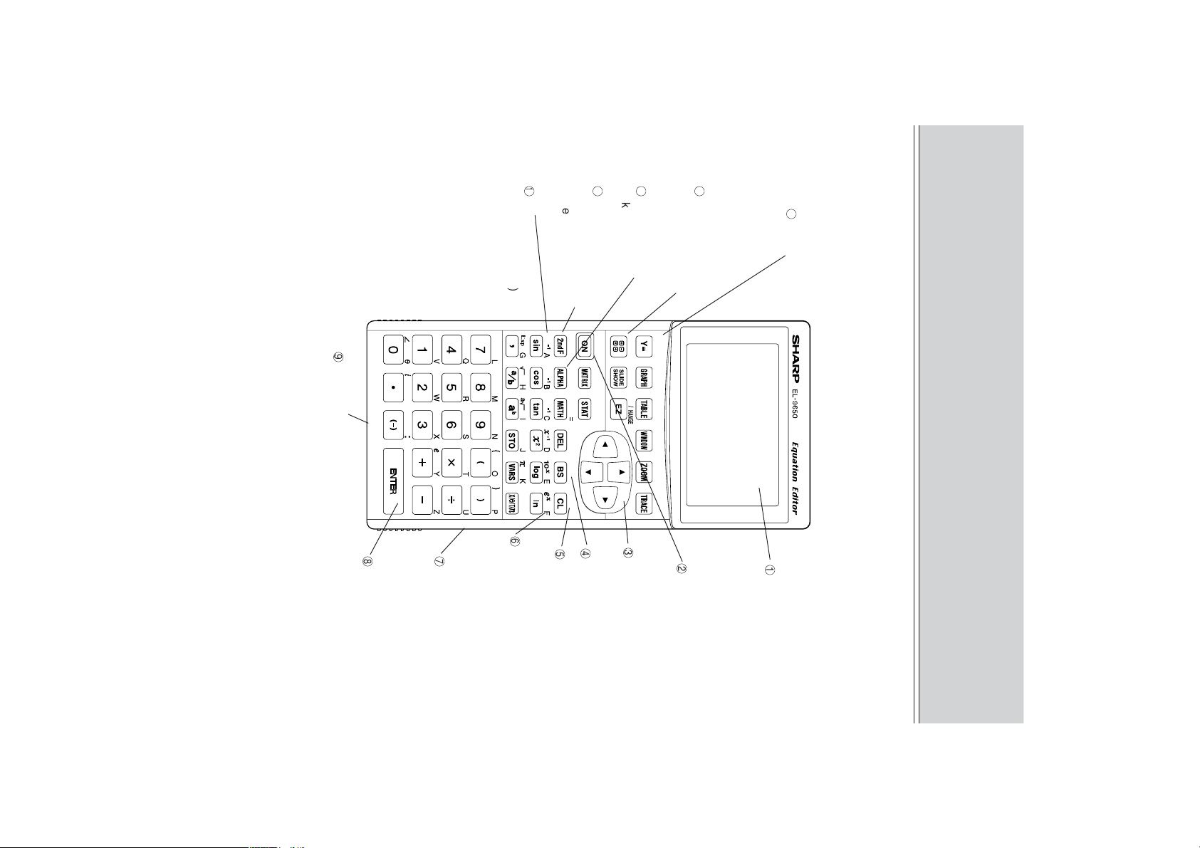
1. Names of Parts
J
Graphing keys
GETTING STARTED
u v w
L4 L5 L6
sin
OFF
ST
SOLVER
AT PLOT
9
Peripheral connection terminal
COMMUNICATION PORT
L
2
SPACE
ENTRY
L3L1
1
LIST
ANS
8
Calculation execute key
FI
EXE
NANC
E
7
Reset switch (on the
back of unit)
cos
A LOCK
PRGM DRAW
CLIP
TOOL
tan
RCL
OPT
ION
INS
SET UP
QUI
T
SHIFT CHANGE
6
Alphabet key (printed in blue)
5
Clear/Quit key
3
4
Cursor movement keys
Set up key
SPLIT
TBLSET
SUB
FORMAT
CALC
2
Power supply ON/OFF
key
GENERAL INFORMATION
1
Display screen
Page 12
4
6
7
8
9
F
G
H
I
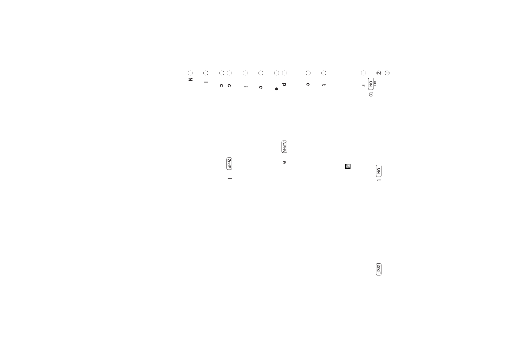
required since all memory contents will be deleted when pressing the reset switch.
executing calculations.
screen which performs numerical calculations or calculations using functions.
Alphabet specification key: Used when specifying an operation printed in blue
Normal function calculation screen selection key: Used when selecting the
in mustard-yellow above a key (upper left).
above a key (upper right).
cables or a PC link cable (not a power supply).
Secondary function: Used with
Secondary function specification key: Used when specifying an operation printed
Calculation execution key: Used when specifying calculation commands and
Peripheral connection terminal: Terminal used when connecting separately sold
Alphabet key: Used with
Reset switch: Used when replacing batteries or when errors occur. Caution is
Å
5
(this may vary according to setting or display screen). These keys are also used
when selecting menus.
format of this graphing scientific calculator.
programs, etc., or when returning to the previous screen. This key is also used when
clearing errors.
Set up key: Mode setting key that determines the calculation method and display
Clear/Quit key: Used when clearing numerical values, calculation commands,
bers. The cursor is indicated using “_” when there is no number or character. The
cursor is indicated using a flashing “
2. Function of Each Part
1
2
3
n
Cursor movement keys: Specifies location to input/correct characters and num-
Display screen
Power supply ON/OFF key: Press
to turn off the power supply.
GETTING STARTED
Ï
2
to input secondary functions.
to enter letters.
” when overlapping a number or character
˚
to turn on the power supply. Press
Ï
Page 13
<Example>
Operation of
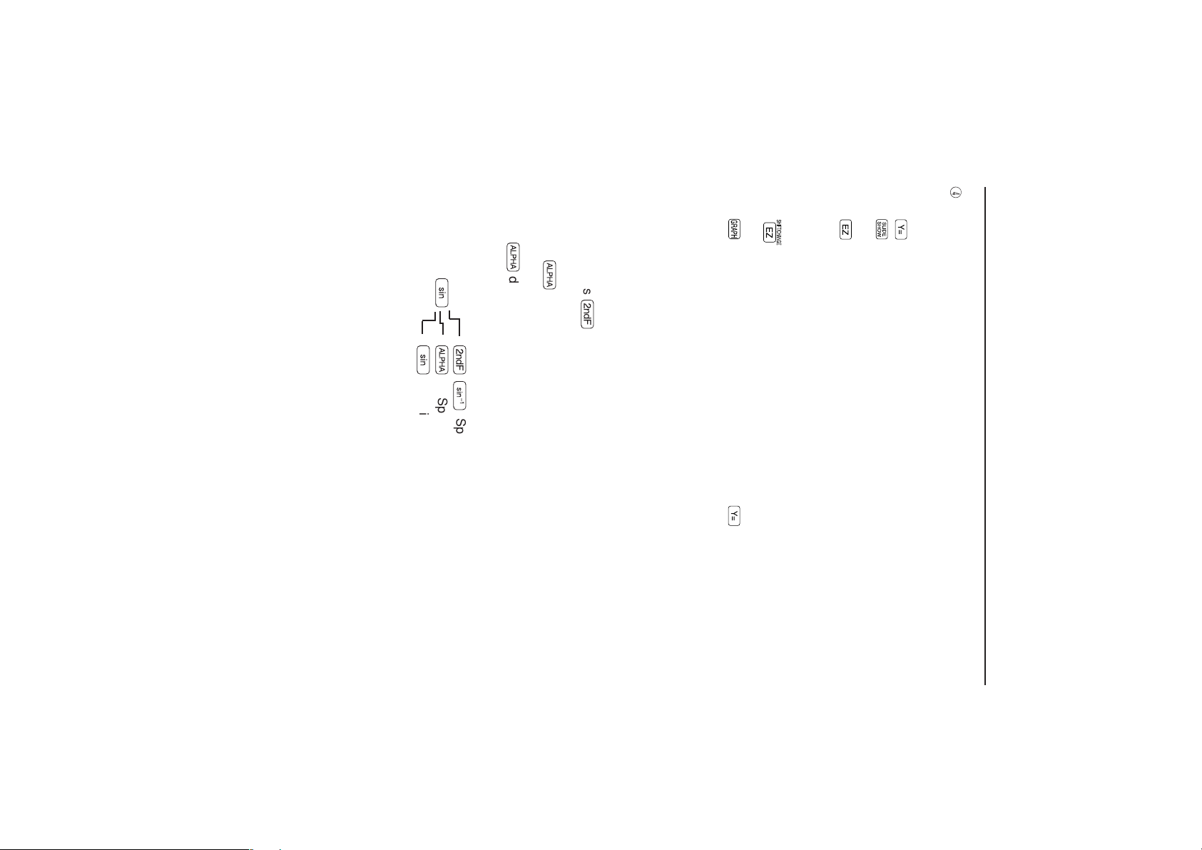
3. Explanation of Keys
• Most keys have more than two functions.
• To use a function printed on a key, simply press the button.
• To specify a function (secondary function) printed in yellow above a key or on the
• To specify a function a character printed in blue on the upper right side of a key,
• : This function is used for studying graphs and to aid understanding.
•
upper left, press
press the
However, there are exceptions to this rule, as in the Menu selection screen, etc.,
where
•
•
J
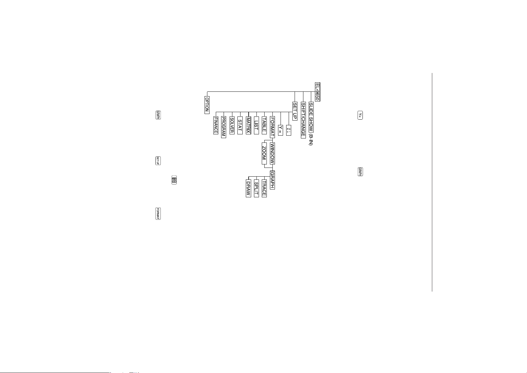
Graph related keys:
Various settings for graphing can be made using the group of keys indicated in the
box.
•
Å
sÅ
sin
-1
A
▼
▼
▼
Ïz
s
: Specify sin
A : Specify character A
does not have to be pressed first.
Å
key first.
Ï
first.
: Draws a graph using the formula inputted in .
: The user can move graph curves and change formats directly with a touch
(For details, see CHAPTER 4 “15. Useful Functions” on page 124.)
of a pen (For details, see page 229).
: Introduces the user to a mode where expansion and reduction of the
graphing screen, input of main functions and graphing settings can be
performed with ease.
: Used to open the formula input screen for drawing graphs.
(For details, see page 221.)
: Specify sin
3
-1
GETTING STARTED
Page 14
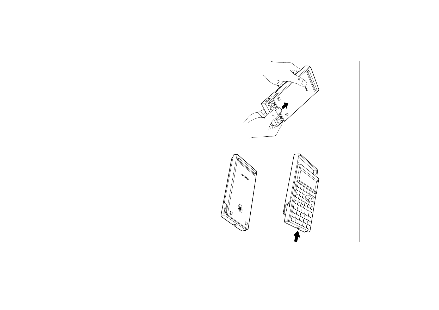
CAUTION
Be careful not to drop the touch-pen when removing the unit from its protective cover.
To open the cover:
4. Using the Protective Cover
GETTING STARTED
4
When not in use:
When in use:
Page 15

(1) Inserting batteries
3. Close the battery cover.
The unit is automatically reset when closing the
battery cover. The display “WAIT” will appear
while the unit initializes settings.
Since the cover also functions as a reset switch,
power will not turn on unless the cover is
attached.
5
Make sure that the tab that was pulled when
opening the cover is inserted completely and a
snapping sound is heard.
Do not remove the label since it
contains backup battery for
memory protection.
the correct direction.
2. Insert batteries as shown in the
Be careful to insert the batteries in
diagram to the right.
down on the tab then lift up.
1. Open the battery cover located on
To remove the battery cover, pull
the back of the unit.
1
5. When Using for the First Time
2
GETTING STARTED
Page 16
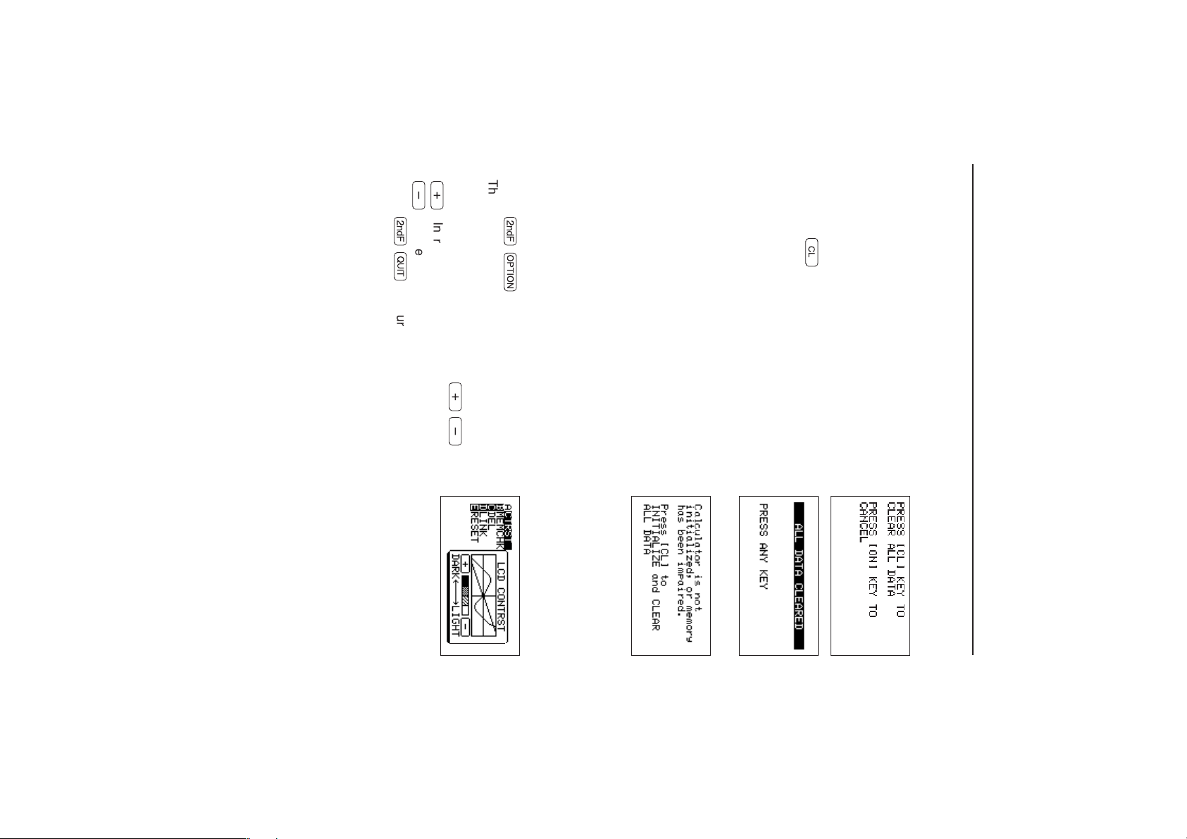
Operation:
3. Press
Ϝ
to return to the previous screen.
6
2. The contrast can be adjusted using
+
-
: Increases the contrast
: Decreases the contrast
+-
.
1. Press
The Optional functions menu will appear (see the
diagram on the right).
Ïq
.
(3) Adjusting the contrast
Display contrast may vary with the ambient temperature and remaining battery
power. Adjust accordingly for the best view.
procedure indicated above.
* The message shown to the right may appear when not
performing the above procedure. To prevent loss of
data, etc., reset the calculator by following the
• Move to the standard function calculation screen by
pressing any key.
• Press the
shown to the right, indicating that all data within the
internal memory of the calculator has been cleared).
¬
key (the display will change to that
• A “WAIT” display will appear momentarily when
unit to clear all data within the calculator’s memory.
pressing the RESET switch. When the display
disappears, the screen shown to the right will appear.
GETTING STARTED
(2) Resetting the calculator
1. Press the RESET switch located on the back of the
Page 17
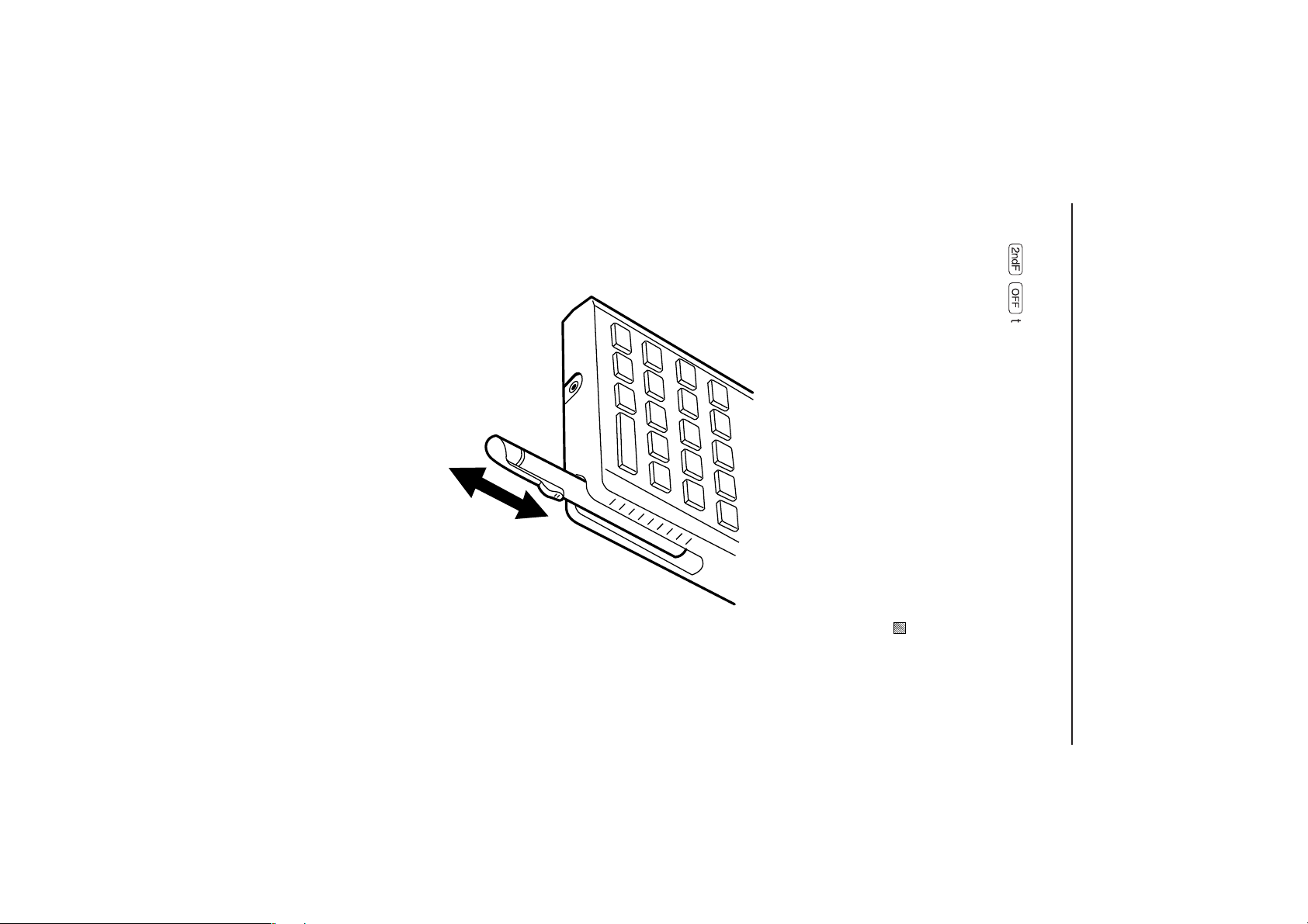
6. Inserting and Removing the Touch-pen
It is possible to store the touch-pen on the side of the main unit when not in use.
7
This function will not operate while executing calculations (flashing “
right side of the screen).
Ï˙
to turn the power off.
GETTING STARTED
” on the upper
(4) Turning the power off
Press
Regarding the automatic power-off function:
The power supply is automatically turned off when there is no operation for a period of
approximately 10 minutes to save battery consumption (the time varies by a few
minutes according to use).
Page 18
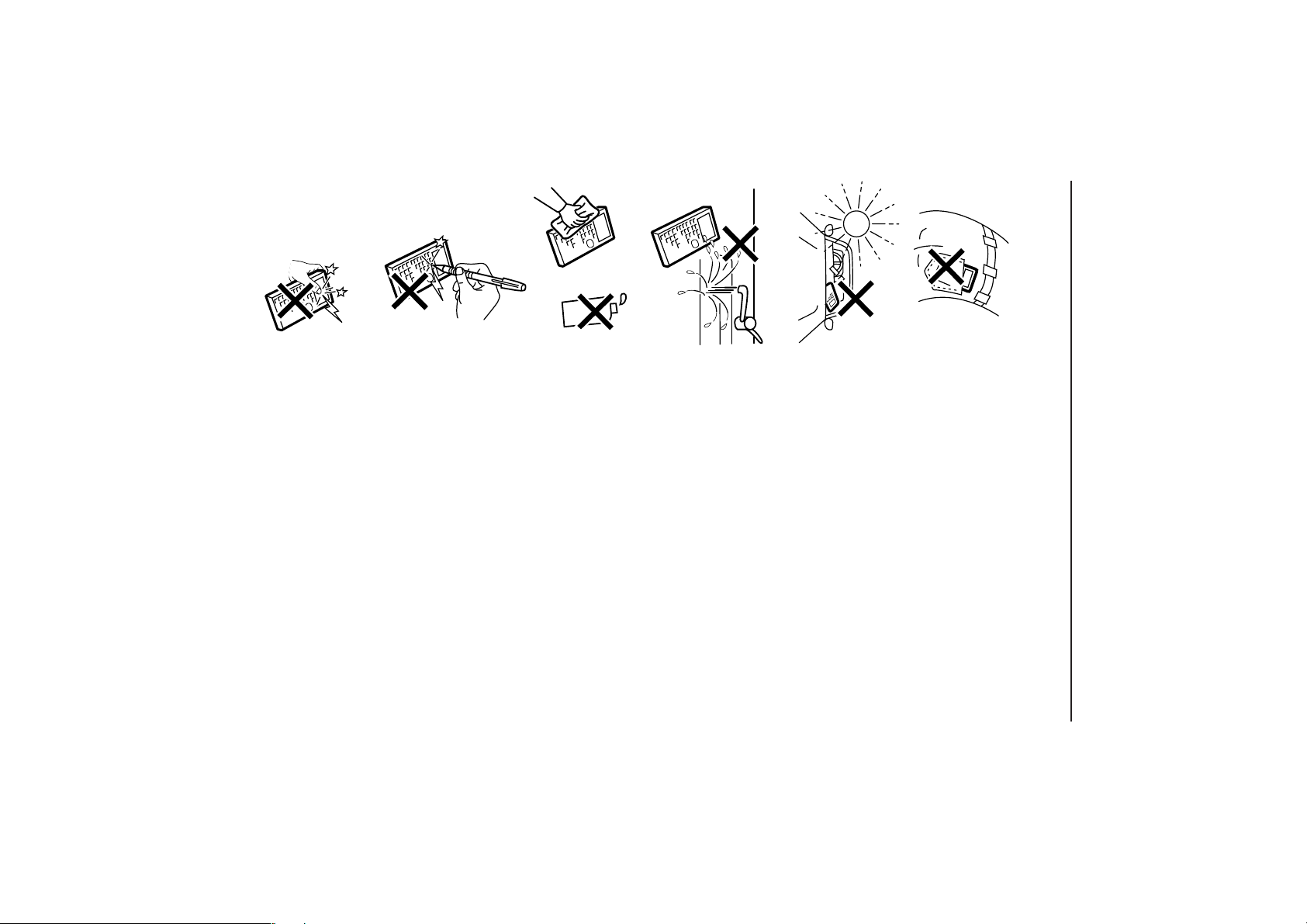
7. Caring for Your Calculator
Keep the calculator away from extreme heat such as
on a car dashboard or near a heater, and avoid
exposing it to excessively humid or dusty environ-
Do not use a sharp pointed object or exert too much
Avoid excessive physical stress.
8
force when pressing keys.
Clean with a soft, dry cloth using no solvents.
perspiration, etc. will also cause malfunction.
Since this product is not waterproof, do not use it or
store it where fluids, for example water, can splash
onto it. Raindrops, water spray, juice, coffee, steam,
ments.
Do not carry the calculator around in your back
pocket, as it may break when you sit down. The
display is made of glass and is particularly vulnerable.
GETTING STARTED
Page 19
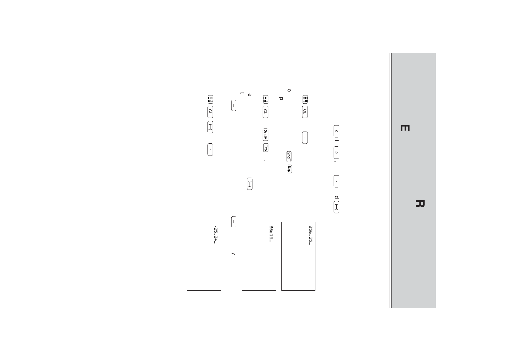
<Example>
To enter “-25.34”
Press
* Using
entering the number.
• To enter a negative (-) number, press
To enter “36×10
Press
<Example>
• To enter an exponent, use
Press
values.
<Example>
To enter “356.25”
procedures described here show how to perform calculations with common math
1. Entering Numeric Values
The number keys (
functions. This chapter also explains the main set-up functions (mode settings).
This chapter describes the basic key operations (input rules) of the calculator. The
¬—
-
to enter a negative number generates an error.
25
.
34.
9
-
is used only for subtraction.
—
before
¬
36
”
Ï
15.
15
Ï
.
¬
356
.
25.
GENERAL INFORMATION
0
to
9
CHAPTER 1
), and
.
and
—
are used to enter numeric
GETTING STARTED
Page 20

10
2. Common Math Operations
The calculator can be used in the same way as a standard calculator for calculations
using common math operations.
<Example>
To obtain the answer of “(100+256)×2÷85–9”
Press
/
Press
calculation appears on the right side of the display below the expression. The display
does not include an equal (=) sign.
85
®
-
¬(
to execute the calculation. The result of the
9.
100
+
256
)j
2
CHAPTER 1
Page 21
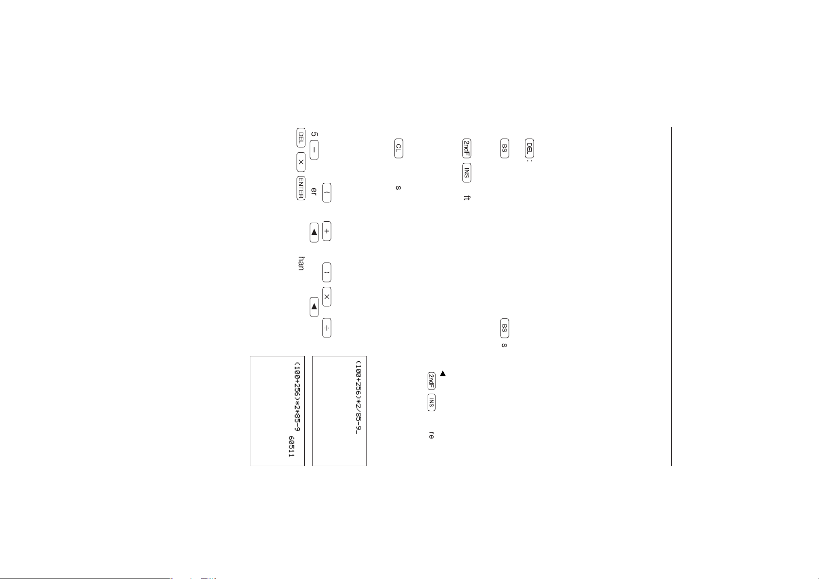
85
dj®
-
9 , enter <<<< <
<Example>
To change “÷” in the expression
to, “×”.
After entering
•
¬
previous calculation.
: clears an entire expression that has been entered and the result of the
* When the INSERT mode is selected, the mode stays active until
again. In the equation edit mode (see CHAPTER 1 “11.Edit Modes” on page 25), the
INSERT mode automatically becomes active.
•
Ï◊
one space to the left and deletes the character or expression entered in that
location.
the left side of the cursor. (When the one line edit mode is selected.)
* When the INSERT mode is selected, the cursor changes to the “ ” symbol.
•
•
d
Ú
the cursor is located is deleted.
sions
: deletes an entry. When this key is pressed, the character or expression where
: moves the cursor backward. Each time
To change a character or expression before executing the calculation, follow the
procedure below.
Move the cursor to the location for correction. The new content will be inserted to the
left of the cursor when entered (during Equation edit mode).
Move the cursor to the character or expression to be changed, and enter a new
character or expression. (When the one line edit mode is selected)
3. Changing Entered Characters and Expres-
11
(
to make the change.
100
+
256
“(
100
)j
+
256)×2÷85–9”
2
/
: after pressing these keys, a character or expression can be inserted to
Ú
is pressed, the cursor moves
GENERAL INFORMATION
Ï◊
are pressed
Page 22
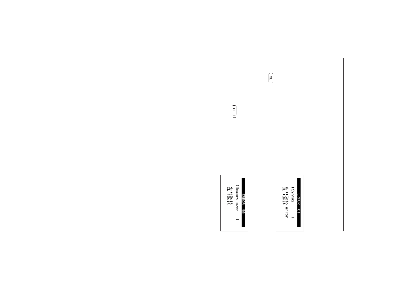
12
Example B: This display indicates that a memory error
has occurred. To correct it, follow the procedure below.
Example C: When any error except one described above occurs, follow the procedure
below.
• Use < or > to move the cursor to the error location, and correct error. (The
• The display will vary depending on the error message.
* For the details of error codes and messages, see APPENDIX “3.Error Codes and Error
Messages” on page 270.
expression on the screen can be changed.)
• Use <, >, or
entered expression will be deleted.)
¬
to clear the error. (The
• Use
to the primary screen. The entered expression will
be deleted.)
¬
to clear the error. (The display will return
below), and stops operating.
The method of correcting an error varies depending on the error code.
Example A: This display indicates that a syntax error
has occurred. To correct it, follow the procedure below.
• Use < or > to move the cursor to the error
location, and correct error. (The expression on the
screen can be changed.)
4. Correcting Errors
When an error is generated, the calculator displays an error message (examples shown
CHAPTER 1
Page 23
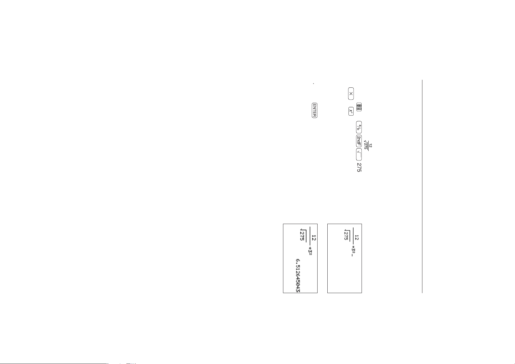
2. Press
1. Press 12
j
5. Using Functions
The following shows an example of a calculation using
functions that are directly accessible from the keys
(functions indicated on keys and secondary functions).
<Example>
To obtain the answer of “ × 3
13
®
.
3 .
;Ï
2
”
275 >>
GENERAL INFORMATION
Page 24
14
ÅY1
executing.
To input a graph equation named “Y1”, press
will display “Y1” on the screen, but an error will be returned when
A®A1
names (L1 to L6) etc., should not be typed out. Instead, the appropriate key must be
pressed or menu item selected.
<Example>
• To change from the ALPHA LOCK mode to the normal mode, press
For successful usage, function names, graph equation names (Y1 to Y9 and Y0), list
cursor changes from “
A” to “_”.)
Å
• Press
Å
mode. In this mode, alphabet letters can be entered
continuously from the keyboard.
A1 2 3
Ï
Ï
to set to the ALPHA LOCK
BCD
θ
.
(2) Entering alphabet letters
<Example>
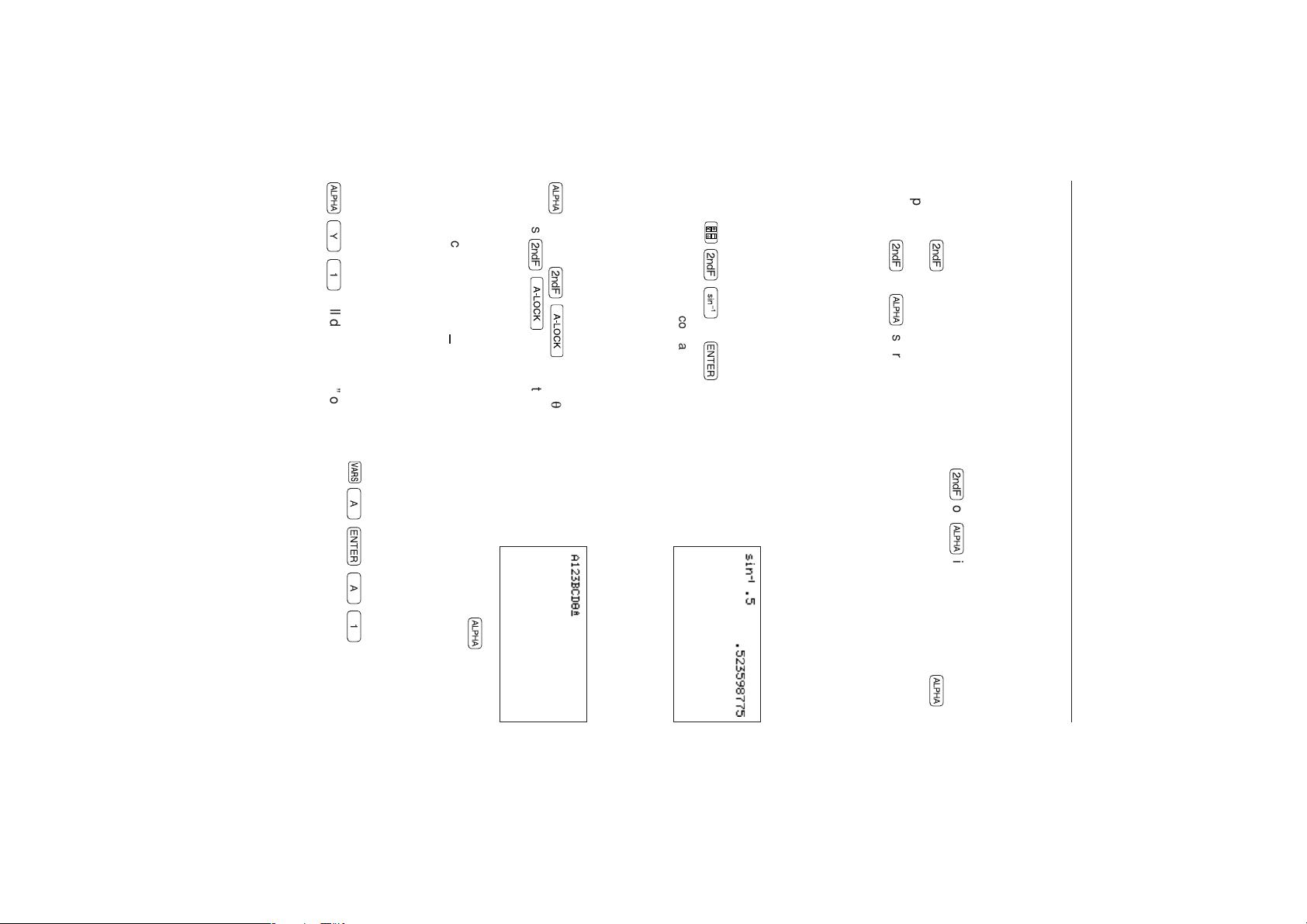
To enter “A123BCDθ”
Secondary function of “sin” key
Press
<Example>
To obtain the answer “sin
Ïz
↑
.5
-1
®
0.5” (Angle mode: Radian)
(1) Using secondary functions (2ndF)
The secondary functions include function entries, menu screen display, and mode
settings.
• The functions and characters printed to the left and right sides above the keys
• When
• When
become active for the next keystroke when
pressed, the characters printed in blue become active.
setting has been changed. (See CHAPTER 1 “12.Display Format of the Cursor
Pointer” on page 32 for details.)
6. Using Secondary Functions (2ndF) and
CHAPTER 1
Alphabet Letters (ALPHA)
Ï
Ï
or
is pressed, the functions printed in yellow become active. When
Å
is pressed, the shape of the cursor changes to indicate that the
Ï
or
Å
is pressed.
. Pressing
(The
Å
is
Page 25
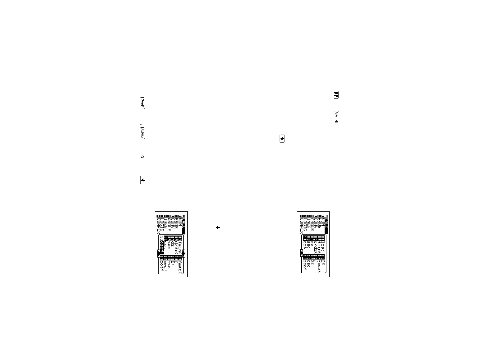
to the sub-menu, and scroll down the sub-menu.
In the example above, press > to move the cursor
to the sub-menu side, and press ≥≥≥
≥≥≥ (6 times). The display should look
like the one shown on the right (items 01 and 02
disappear from the display, and items 13 and 14
appear at the bottom).
Press
advance the sub-menu screen.
• To see how many items are in the sub-menu, move the cursor from the main menu
that there are more items that are not currently shown on the screen.)
however, the number indications are highlighted. This indicates that no function is
currently selected. The sub-menu shows items 01 to 12. The “
• On this display, the highlighted function or mode name (not the alphabet letter or
(In the above example, [A CALC] is currently selected. In the [A CALC] sub-menu,
number) is currently selected.
• The display changes to the screen shown above.
• The main menu lists items A to H (the number of items varies in each menu). Each
item on the main menu has a sub-menu.
<Example>
Press
grouped by function type and item type. Calculations and mode settings can be
executed by selecting appropriate functions.
7. Using Menus
This calculator is equipped with function menus that allow many functions other than
those printed on the keys and main unit to be used. These additional functions are
15
Ï
≥,
Å
≥ or touch
on the screen with the touch-pen to
” symbol indicates
and
≥
.
: This symbol appears when there are more items after No. 12.
Main menu items
GENERAL INFORMATION
Sub-menu items
Page 26
There are three ways to select a menu.
1
2
3
Use <, >, ≥, and ≤, to move the cursor and highlight the selected
function, and press
Enter the letter (A, B, etc.) or number of the selected menu to directly access the
menu. (There is no need to press
Select a menu item by pressing the item on the screen twice with the tip of the
touch-pen provided.
®
.
Å
• Press ≥≥≥ (3 times). The display should
displays the “ ” symbol, there are no more sub-menu
When the screen no longer shows the “ ” symbol but
items below (end of the page). (There are 20 sub-menu
items in the [A CALC] menu.)
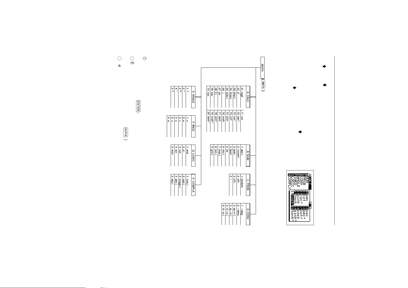
The following diagram shows the main menu and sub-
menu structure described above.
currently shown on the display.
look like the one shown on the right.
•“
CHAPTER 1
” and “ ” symbols indicate that there are more items before and after those
16
.)
Page 27
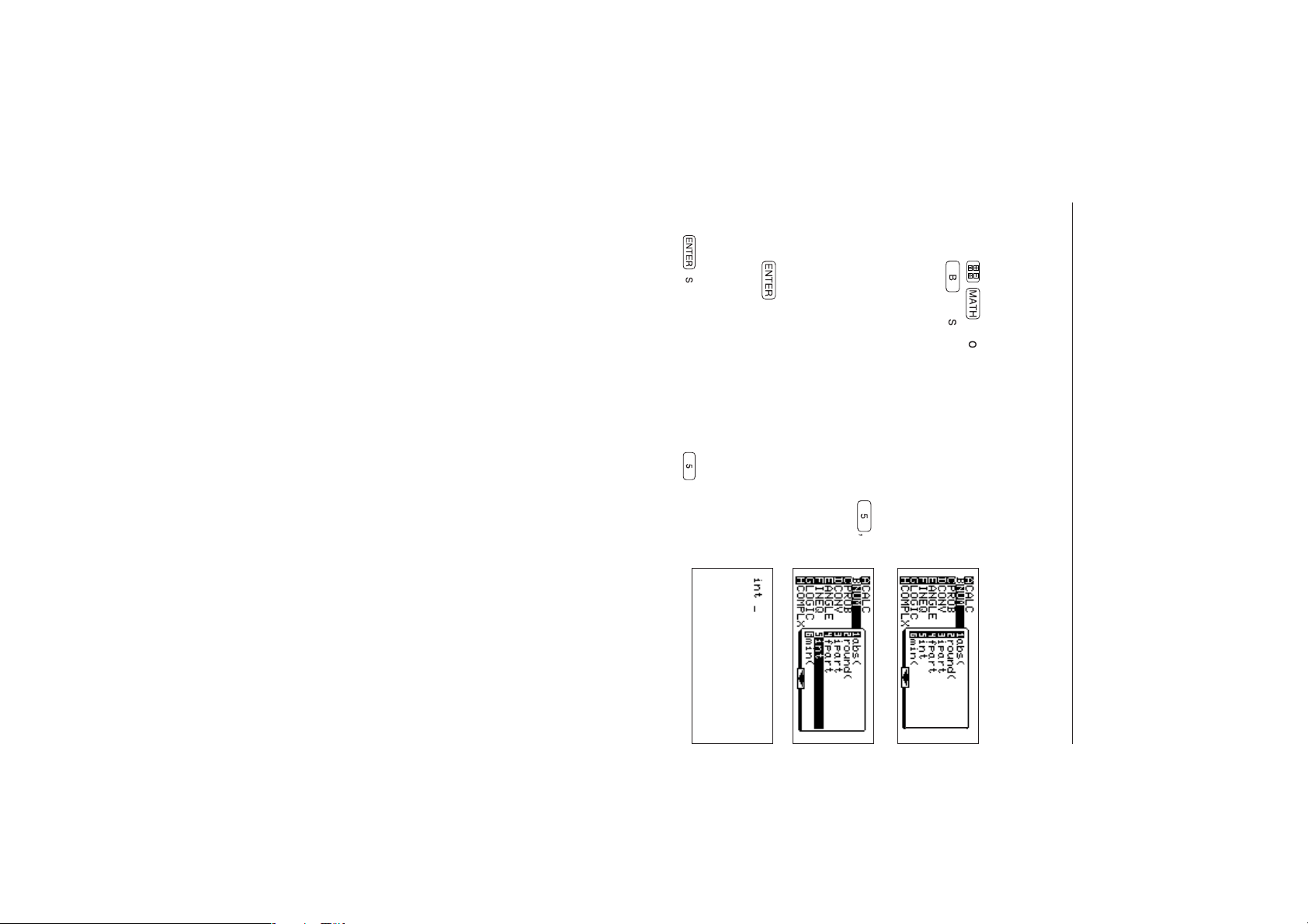
4. Press
* In this calculator, functions are grouped and stored in menus. This allows the many functions
3.
to be used easily.
®
is not necessary when pressing
again.
displayed before the menu screen appeared.
®
The “int” indication appears on the screen that was
*
, or select [5 int] with the touch-pen
3. Press > ≥≥≥≥ (or press
or select [5 int] with the touch-pen).
1. Press
2. Press
touch-pen).
<Example>
To use the “int” function to obtain a whole number (The “int” function is in the [B NUM]
sub-menu of the MATH menu.)
B
≥
(or select [B NUM] using ≥ or the
to open the MATH menu.
17
5
of procedure
5
,
GENERAL INFORMATION
Page 28
18
• The style of
• If display or calculation results are not what is expected, check to see whether there
are errors in the setting by following the chart to the left.
settings.
, in addition to is influenced by .
To view the flow chart:
• SLIDE SHOW is unrelated to the SET UP menu.
• The normal function calculation mode
is influenced heavily by the SET UP
8. Operating Modes
• The EL-9650 has many modes and commands that are related to the display
• Expected results cannot be obtained when errors are made in the default settings.
• Modes that influence various calculations and processes have been organized into a
* In reality, each command and mode are related in a complex manner.
For example, (equation input) and are related. However a vertical line is not drawn on
This is to show the horizontal relationship (modes that have the most influence) in the most
the flow chart.
simple way.
flow chart.
method of equations, graphs, lists, calculation results and key input
CHAPTER 1
Page 29
6
3
2
1
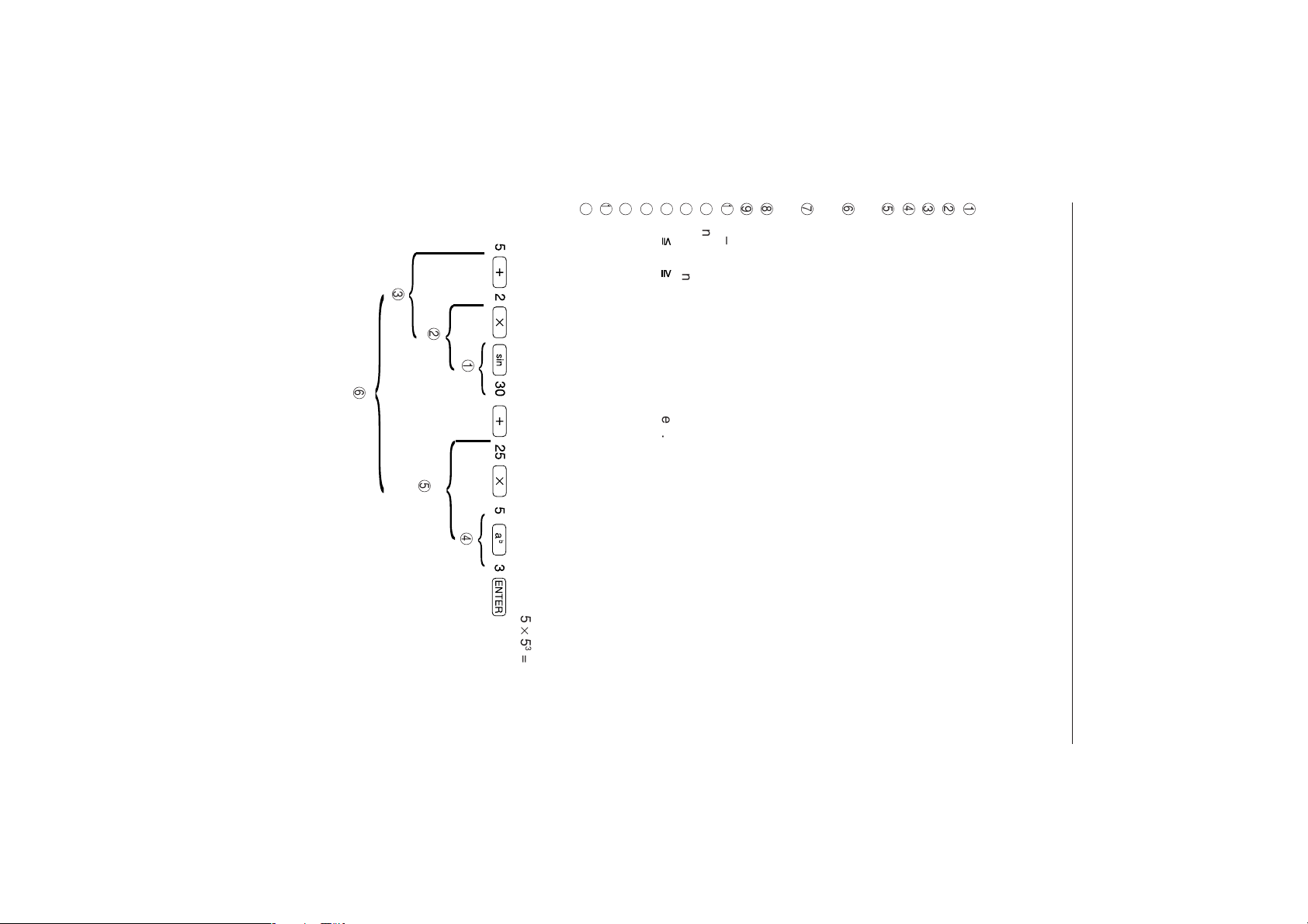
<Example>
The key operation and calculation precedence of 5 + 2 × sin 30 + 25 × 5
M
{, [, STO, etc.
J
I
)K (L }, ]
<,
, >, , ≠, =, → deg, → dms, etc.
G
H
and
or, xor, xnor
F
+, –
9
Permutation/combined functions (nPr, nCr)
function that follows a numerical value (3 cos 20, etc.).
×, ÷
6
Multiplication with omitted “×” commands immediately before a single calculation
Single calculation functions that are irnmediately after a numerical value (sin, cos,
tan, sin
-1
,cos
-1
, tan
-1
, log, 10
x
,In, e
x
, ◊,abs, int, ipart, fpart, (–), not, neg etc.).
7
8
4
5
Single calculation functions immediately before a numerical value (X
Exponential functions (a
Multiplications with omitted “×” commands immediately before variables such as π or
stored memory and 2π, 2A, etc.
b
,
a
◊ etc.)
Complex angles (∠)
Fraction calculations (a/b)
• This unit is equipped with a function that detects calculation precedence.
• The calculation precedence is as follows:
1
2
3
9. Precedence of Calculations
19
5
4
GENERAL INFORMATION
2
3
=
, X
–1
, !, °,
r
,
g
).
Page 30
20
[3 Grad]: Set to gradient
The above display will appear when
menu is used for displaying the current settings, the menus that can be set are B
through G, with sub-menus for each. The functions of these are explained below.
[B DRG]: Used to set the angle unit (default setting: Rad)
[1 Deg]: Set to degree
[2 Rad]: Set to radian
}
The relationships are:
Ï
are pressed. Since item A of the main
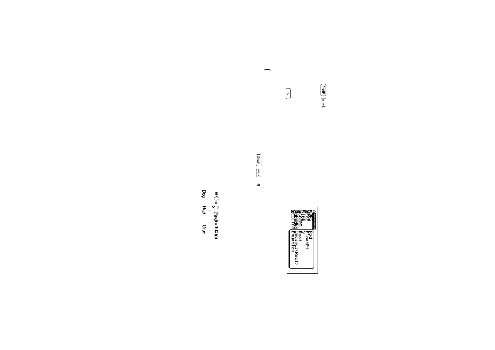
(2) SET UP menu
* “A” is highlighted and current settings are displayed when
Contents displayed on the right side of the screen when
selecting [A] are the current settings.
entering the SET UP mode. In this case, it is not necessary to
press
A
.
(1) Checking SET UP contents
Press
Ï
.
• Be sure to set the SET UP mode according to desired calculations and graph
plotting since there may be differences in the results depending on the set conditions
of SET UP.
10. SET UP Menu
• SET UP is a function that sets input and display methods.
• Please select each method according to use.
CHAPTER 1
Page 31

Now try the same calculation in the Deg mode.
3. Press
touch-pen.
2. Press
4. Return to the normal function calculation screen by
5. Press
As can be seen above, the results vary according to
the set up, even when performing identical calculations.
Now the Deg mode is set.
pressing
1. Press
6. Press
5. Return to the normal function calculation screen by
This is because Rad is the default setting.)
pressing
3. Press
4. Press
Now the Rad mode is set. (When you set for the first
time, Rad is already highlighted when moving the
cursor pointer from the main menu to the sub-menu.
touch-pen.
1. Press
Delete the display screen completely.2.Press
The units of angle are according to the ones chosen in the SET UP. Be careful since
the calculation results may differ unless the angle units are set properly.
<Example>
Calculate “sin π/4” using the Rad mode.
21
s
(Ï
,
Ϝ
π/
, or
¬¬
4
)®
.
.
Ï
B
1
or touch the [B DRG] display using the
or touch the [1 Deg] twice.
.
s
(Ï
or
¬¬
π
.
/
4
)®
.
B
2
or touch the [2 RAD].
Ï
or touch the [B DRG] display using the
¬
.
.
GENERAL INFORMATION
Page 32

22
8. Press 1
[E COORD]: Used to set the coordinate system of
graphs (default setting: Rect)
[1 Rect]: Rectangular coordinates
[2 Param]: Parametric equation coordinates
[3 Polar]: Polar coordinates
[4 Seq]: Sequential graph coordinates
6. Touch [2 2].
7. Return to the normal function calculation screen by
pressing
/
3
®
.
.
3. Press
4. Touch [3 Sci].
5. Press
Now the method for displaying results is set.
C
D
or touch [D TAB].
Ï
or touch [C FSE] using the touch-pen.
.
Clear the display screen completely.2.Press
Set to TAB 2 in the Sci mode then execute “1 ÷ 3”.
1. Press
¬
.
[D TAB]: Specifies the number of decimals (default setting: 9).
TAB 0 to 9 can be set from submenu options.
<Example>
is specified in [D TAB], which is described later.
CHAPTER 1
[C FSE]: Used to set the display method of calculation results (default setting: FloatPt)
[1 FloatPt]: Floating point method
[2 Fix]: Fixed decimal point method
[3 Sci]: Exponential method (✳✳✳E
[4 Eng]: Engineer’s exponential method (exponentials are in multiples of 3: ✳✳✳E
In [2 Fix], [3 Sci], and [4 Eng], the answer displays using the number of decimals set by
TAB.
CAUTION
When FloatPt is selected in this menu, FloatPt is given priority even if the number of decimals
✳✳
)
multiples of 3
↑
✳✳
)
Page 33

[5 r ∠θ] (complex): Displays results using complex polar numbers (complex number
produce different screens according to the SET UP
settings.
6. When
the right for polar coordinate graphs will appear.
Even with an identical key ( ), the unit will
[F ANSWER]: Used to set the display method and mode of results (default setting:
Decimal Real)
[1 Decimal] (real): Displays results using decimals (real number mode).
[2 Mixed] (real): Displays results using mixed fractions (real number mode).
[3 Improp] (real): Displays results using improper fractions (real number mode).
[4 x±yi] (complex): Displays results using complex rectangular numbers (complex
4. Press
5. Touch [3 Polar].
3. Press
1. Press
2. Press . (Keys to be used when inserting functions
<Example>
This example shows the difference of the formula input screen for polar coordinates
and rectangular coordinates.
or writing subsequent details.)
23
number mode).
mode).
E
is pressed, the formula input screen to
or touch [E COORD] with the touch-pen.
Ï
.
Formula input screen of
rectangular coordinates
¬
.
GENERAL INFORMATION
Page 34

24
[1 Equation]: Used to set to the mode where formulas can be input as they appear.
[2 One line]: Used to set to the mode where the input numbers can be input and
displayed on one line.
[G EDITOR]: Used to set the input method of numerical formulas (default setting:
6. Return to the normal function calculation screen by
as in the formula.
pressing
Equation).
. The answer is shown using fractions
4. Press
5. Press
pen.
3
or touch [3 Improp] (real) twice.
2. Press
3. Press
decimal (real).)
F
Ï
¬
or touch [F ANSWER] with the touch-
.
1
1.
Ï
(Check that [F ANSWER] is set to
;
3
®
.
The SET UP condition for B to E is Rad, FloatPt, 9, and Rect respectively.
CHAPTER 1
<Example>
This example shows the differences in the display method of results for decimals and
improper fractions using “1 / 3”.
NOTE
Page 35

25
The following functions are displayed two-dimensionally on the display.
a/b,
keystroke is displayed on the screen. (The screen may display several entries all at
once.)
To enter an expression, use number keys, arithmetic keys, other function keys and
cursor keys (<>≥≤).
the internal processing to locate the display position of the variable or function. There-
fore, the calculation speed is slightly slower. The calculator memory retains a maximum
of three keystrokes. Therefore, keys may be operated before the input of the previous
, , e
x
, 10
x
, x
2
, x
–1
, a
b
, abs, ∫dx (integral function), ( ), [ ], etc.
(1) Equation edit mode
Expressions are displayed two-dimensionally in commonly used mathematical expres-
sions.
In the equation edit mode, expressions up to 114 bytes can be entered and the display
shows up to 8 lines of an expression and a calculation result. (It is not possible to input
an expression exceeding this limit.)
In the equation edit mode, each key input is displayed after the calculator completes
* The calculation speed of the equation edit mode is slower than that of the one-line edit mode
due to extra internal processing.
11. Edit Modes
Expressions can be entered either by the one-line input method or the equation input
method.
In the one-line edit mode, the EL-9650 is used in the same way as a standard scientific
calculator. The equation edit mode allows entries of fractions and functions such as
powers, roots and constants in a straightforward sequence. (Matrices cannot be
entered in a straightforward sequence.)
To set a mode, select : [Equation] (equation edit mode) or [One line] (one-line edit
mode) by using [G EDITOR] of the SET UP function.
If an expression has been already entered and is displayed, the expression cannot be
changed by switching the input mode.
(If the EDITOR setting is changed in the middle of entering an expression, the portion
of the expression that has been entered will be deleted.)
GENERAL INFORMATION
Page 36

• Use
• When entering a new expression or making a correction, the cursor changes into
“
”:This indication is always accompanied by the “ ” cursor, and indicates the
input location. It appears after the fraction key
pressed. It indicates the location where the next number or function is to be
entered.
appears in front of an expression.
“ ”: Indicates a cursor that allows insertion of a character or function. The inserted
“
”: Cursor that appears when inserting. Insertions of text and functions are made
to the left of the cursor (flashing).
character or function appears on the left side of the cursor. This input cursor
appears in front of a structural function or after an argument. The cursor also
one of the following four types depending on the input position.
“_”: Indicates the location where a new entry can be made. (Blank space on the
right of the cursor)
d
or
Ú
• If the entered expression has more than 22 characters, the screen scrolls to the left.
• In the equation edit mode, the INSERT mode automatically becomes active for key
entries. (There is no need to press
3. Press 22
>
≥ A06
≥07®
;Ï
to delete a function or character.
0 ≤ 4 > 2
121 >>
.
the equation.
The sizes of other function indications are the same as those displayed in the one-line
edit mode.
<Example>
To obtain the answer of “
1. Press
2. Press
edit mode.
Ï G1
¬
to return to the primary screen.
to set to the equation
Of these, the sizes of the parentheses ( ) and brackets [ ] will be changed depending on
CHAPTER 1
26
;
or power key, etc. is
Ï◊
to set to the INSERT mode.)
”
+
3
Page 37

↓
®
↓
Insert
+
<<
↓
<Example>
To enter the expression “ ”, and move the cursor.
(SET UP F and G setting: Mixed (Real) and Equation)
Press
¬
1
;
27
↓
®
2
↓
Insert 4
j
3 >
®
When the key is pressed,
the calculation result is
displayed. The cursor
cannot be moved back to
the expression with <,>,≤, or ≥.
<<<<.
→
+
2
;
5.
GENERAL INFORMATION
↓
Page 38

6. Press 2
“2×” is inserted.
5. Press <<<<<.
4. Press
7 >
3. Press 1
“1+” is inserted.
2. Press <<<<.
Here, we will input “
1. Press
CHAPTER 1
<Example>
28
j
.
¬
;
3
5.
+Ï
+
.
¬
5
;
” first and then “
7.
”,
and move the cursor.
Page 39

All arguments are displayed with “ ” as in the diagram on the right when inputting
integrals (∫). “
“ ” will appear for temporary use when there are no
arguments.
“
added.
” will automatically disappear if an argument is
↓
” will also disappear if an argument is input.
Input
;
Press
¬
1
+
2 <.
<Example>
Press
¬
1
+
5
;
• Parentheses are automatically placed when inputting structured functions such as x
The following eight types of functions are enclosed within parentheses: a/b,
x
2
, x
x
-1
-1
, a
, a
b
b
, etc. (with the exception of abs).
, ∫dx (integral functions)
29
↓
Input
;
Press
¬
1
+
52 <.
→
6 >.
Input
These parentheses are automati-
cally placed.
→
, , e
,
GENERAL INFORMATION
x
2
,
Page 40

8
∫dx (integral) :
7
abs :
≥B1—
≥A06
5
≥ A07
3 6 >
6
10
x
:
Ï
5 >
5
e
x
:
Ï
2 >
4
a
b
:5 6 3 >
3
:
Ï
2 6 >
2
:
3
Ï
1 2 1>
1
a / b: 5
;
2 >
Examples for inputting structured functions are shown below. For all other functions, the
operation will be the same as the one line input method.
CHAPTER 1
30
0 ≤ 3 >
Page 41

31
2. Return the display to the primary screen by pressing
3. Press
Each line can contain up to 22 digits and signs. The
portion of an entry that exceeds this limit will be dis-
played from the beginning of the next line.
See CHAPTER 3 on page 49 for the method of entering functions.
6
))+
Ï(
3 3
3 2
®
;(
.
3
Ï
2 4
¬
1. Press
* The settings can also be made from the menu by using the cursor keys ( <>
≥≤ ) or pen touch.
Ï G2
to set to the one-line edit mode.
To obtain the answer of “ ” (SET UP B to F settings: Deg, Float Pt, 0, Rect,
and Decimal(Real))
(2) One-line edit mode
Expressions are entered with number keys, common math function keys and other
function keys in the same manner as with a standard calculator.
The screen displays a maximum of eight lines for an expression and a calculation
result. Expressions up to 160 bytes can be entered. Only a limited number of digits and
signs are displayed.
<Example>
.
GENERAL INFORMATION
Page 42

• A different cursor may appear on the graphing screen.
4
: This cursor appears while editing numerical formulas that have been input as is. It
is a flashing inset cursor that appears at the end of arguments and in front of
structured functions.
3
: The flashing insert cursor appears when entering the insert mode by pressing the
◊
cursor).
MATRIX screen, etc.
formula edit mode.
: Cursor that appears during the normal function calculation mode and input screen,
: The cursor of
When pressing
1
2
while editing numerical formulas (insertions are made to the left of the
1
will change to this flashing cursor when entering the numerical
2
–
Normal
When pressing
A
–
–
1
Normal input
Whole character
12. Display Format of the Cursor Pointer
• The display format for the cursor pointer depends on the mode settings and screens,
• The conditions and display formats are as follows:
CHAPTER 1
even when performing the same operations.
32
2
Edit
3
Insert
4
Half-character
Page 43

*
Press
*
Press
Press
Å
Å
Ï
≤ to jump to the previous page of the sub-menu.
≥ to jump to the next page of the sub-menu.
≥ to jump to the last item of the main menu or sub-menu.
Press
Press
Press
Ï
Ï
Ï
< to jump to the front of the numerical formula.
> to jump to the end of the numerical formula.
≤ to jump to the top item of the main menu or sub-menu.
It is possible to jump to the top line or the end by pressing
cursor movement keys.
(3) Jumping (
Ï
<,
Ï
>,
13. Moving the Cursor
(2) Moving the cursor vertically (≤≥)
It is also possible to move the cursor vertically in the main menu and sub-menu of
the menu screen.
When in the one line input mode, it is possible to move the cursor vertically when
there are two lines or more. In the input screen for as is formulas, it is possible to
move the cursor between arguments of fractions, exponents, and integral functions.
one digit at a time for numbers and characters. It is possible to move the cursor
along the graph line in the graph display screen during the tracing.
(1) Moving the cursor horizontally (<>)
The cursor can be moved along the input line. It is also possible to switch from the
main menu to the sub-menu and vice versa in the menu screen. The cursor moves
33
Ï
≤,
Ï
Ï
≥ )
before using the
GENERAL INFORMATION
Page 44

• To cancel the reset operation , press
Pressing any key will move on to normal function
calculation screen.
3. To clear all memory data, press
This display will appear after “WAIT” appears
momentarily.
¬
• You can either press the reset switch located on the back of the unit or select the
2. The screen shown on the right will appear.
* Use the enclosed touch pen to press the reset switch. Do not use sharp points such as
mechanical pencils, as this may damage the switch.
(2) Using the reset switch
The reset switch is located on the back of the unit.
1. Press the reset switch on the set screen.
* Take care since resetting the unit will delete all memory data.
reset function in the menu.
(1) Reset
• Use the reset function in case a malfunction occurs, if you want to delete all data, or
want the values for various modes to return to the default settings.
14. Resetting the Calculator
CHAPTER 1
34
˚
.
.
Page 45

Initializing settings:
1. Press
2. Press
3. Press
Press any key to return to the normal function calcula-
tion screen.
2. Press
1. Press
All memory: This reset function initializes the memory contents and settings.
Deletion of all set memory:
(3) Select RESET from the menu
This reset function is used when deleting all memory data at one time or when initializ-
ing settings with memory undeleted (SET UP setting contents, etc.).
There are two types of resetting:
default set: This reset function initializes only the settings, but does not delete the
35
®
ÏqE1
.
.
¬
.
2
.
ÏqE
memory.
.
GENERAL INFORMATION
Page 46

36
CHAPTER 1
Page 47

(1) Using the touch-pen on the menu screen
2. Press
The highlighted menu is the selected menu.
indicates that there are more sub-menu items after
number 12).
[A CALC] of the main menu will be highlighted and
options 01 to 12 of CALC will appear on the right
side of the screen (“
1. Press
(Manual key entry must always be used for turning
on the power supply).
some screens.
• Solver Function (For details, see CHAPTER 9 on page 211.)
• SLIDE SHOW Functions (For details, see CHAPTER 10 on page 221.)
1. Pen-touch Operations
• This function is valid for most screens; however, this function will not operate on
• This function allows operations identical with manual key entry, such as selecting
menus, changing screens, moving the trace cursor, etc. by touching the screen with
the attached pen.
• SHIFT/CHANGE Functions (For details, see CHAPTER 11 on page 229.)
This section explains the unique functions of the EL-9650.
• Pen-touch Operations
37
≥
.
” on the bottom of the screen
˚
.
A
UNIQUE FUNCTIONS
CHAPTER 2
UNIQUE FUNCTIONS
Page 48

38
7. The highlighted [7 max(] shows that it has been
To confirm the [7 max(] command, touch the
selected.
highlight again.
≥ of manual entry. The secondary screen will display
sub-menu items 4 - 9 when
Ï
≥ is pressed).
* In other words, pressing advances the sub-menu by
disappear and will appear on the upper right
side of the screen.
( indicates that there are more menus before this
screen.)
one page (although the ≥ advances one line at a time,
specifying using the touch-pen is equivalent to
Å
6. The screen will change to that shown on the right.
Sub-menu items 7 to 9 will be displayed. will
5. Touch .
( indicates that there are more sub-menu items
following number 6.)
CHAPTER 2
4. Next, touch [B NUM].
The screen will change to that on the right.
right
([D CONV] is highlighted, and sub-menu items of
[D CONV] are shown on the right).
3. Touch [D CONV] of the main menu using the
Check to see that the screen changes to that shown on the
attached pen.
D”
D’
D
C
B
Page 49

39
• The touch-pen operation should be performed without exerting force.
• The display screen is made of glass and film and may break if too much force is
• Always use the attached touch-pen when using the touch-pen operation. Using
• Because there will be a minor difference in the actual display area and the touch
Since highlighted items are not confirmed, they can be corrected by simply pen-
If an item has been confirmed by pressing
pressing
touching the correct item.
area depending on the viewing angle and operating conditions if you make an error,
follow the procedure below:
applied.
metal or sharp objects will scratch the screen and may result in malfunctions.
¬
, then reenter.
®
, delete the confirmed command by
Cautions when using the touch-pen operation:
* The screen is not exactly the same as others.
>
D
®
......................
®
...............................................Pen-touch [7 max(] ........ Screen F
B
↓↓ ↓
↓↓ ↓
↓↓ ↓
Å
........................
........................
≥....>≥≥≥≥≥≥ ..... * Pen-touch ............Screen D”
D
B
.................................................Pen-touch [D CONV] ..... Screen B
.................................................Pen-touch [B NUM] ........ Screen D
previous screen or executing calculations.
(For manual key entry, press
↓↓ ↓
≥
is highlighted.)
®
When performing touch-pen operations in the menu screen such as above, the first
pen-touch highlights the selection (indicates that the item has been selected) and the
second pen-touch confirms the selection/function for transferring commands to the
when [7 max(]
8. The screen will return to the display it had before
opening the MATH menu and the previously
selected command is transferred.
F
UNIQUE FUNCTIONS
Page 50

<Example>
The touch-pen operation for changing “56×42”, which
has completed calculation of “56×42 = 2352”, to “36×42”
is explained here.
1. Touch the area above the answer (2352 on the
diagram to the right) with the touch-pen.
5. “56×42” will be calculated when pressing
4. Press
shown to the right.
3. Touch “3” on the screen using the pen.
The cursor will flash on top of the “3” indicating the
edit mode (it is now possible to correct the “3”) as
Press
<Example>
The touch-pen operation for changing the “3” of entered “56 × 32” to “4” is explained
here.
1. Initialize the screen.
2. Input
screen
d4
.
5
¬
,
6
.
,
j
,
3
,
2
CHAPTER 2
(2) Using the touch-pen on the normal function calculation
40
®
.
using manual key entry.
Page 51

41
In other words, when a calculation has already been executed, it is possible to call out
the formula by touching the area above the answer with the touch-pen.
3. Select “5” using the touch-pen as above. Change the
number to “3” then press
®
to execute calculation.
2. This will display the previous formula one line below
the answer (the cursor is positioned in a location
before the calculation).
UNIQUE FUNCTIONS
Page 52

42
• Pen-touching on a full screen graph, as above, is considered here.
* Operations differ when in the normal mode and trace mode. Both are explained below.
* For more information on graphing functions see CHAPTER 4 on page 79.
5
Pen-touch the graph curve
(no formula display)
4
Pen-touch the graph curve
(formula display graph)
6
Pen-touch the cursor
coordinates display
1
Pen-touch the numerical formula
2
Pen-touch an area unrelated to
graphs or formulas
3
Pen-touch the X or Y axis
• The touch-pen is used on the graph screen to specify cursor location (also used to
selection.
select formulas when tracing).
•“
• The selected area when pen-touching on the graph screen is displayed using “
function calculation screen, and touching the same area once more confirms the
• In the graph screen, it is possible to easily set the direction and amount of graph
shifting using the SHIFT/CHANGE function, etc. as described later, specify tracing
locations, and enlarge and reduce screens using the touch-pen operation.
CHAPTER 2
(3) Using the touch-pen on the graph screen
” appears when touching the graph screen with the touch-pen as on the normal
”.
Page 53

When the graph is in the trace mode:
• Since the split screen (
side of the screen (graph) moves the cursor in the same manner as the previously-
mentioned trace mode. Pen-touching the right side of the screen (list screen or
formula screen) changes graph formulas and moves the cursor pointer to the graph
curve position that corresponds to the list position.
pointer).
when pen-touching the second time is fixed as shown
below (“ ” is the boxed area and “ ” is the cursor
* The location where the cursor pointer appears. The
onscreen “ ” is displayed using a 8 × 10 dot configura-
tion. The relationship of the cursor pointer and the “ ”
5
: When using the same procedure as in
Touching within the “ ” moves and displays the cursor pointer within the “ ” and
the “
along with the cursor movement will change to that of the graph line newly moved by
the cursor pointer.
1
4
to
: “ ” will appear with the first pen-touch.
Touching within “
• When not in the trace mode, it is possible to display and move the cursor pointer to
the specified location for all selections.
3
,
” disappears.
6
: “ ” will appear with the first pen-touch.
” deletes “ ” and returns to the previous graph mode.
Ï
) is always in the trace mode, pen-touching the left
• The cursor pointer will appear in a point (fixed)* within “
When the graph is in the normal mode (non-trace mode):
•
2
touch to the same area.
to
5
: Press anywhere and “ ” will appear with the first pen-touch.
43
4
, the formula displayed on the upper left
” with the second pen-
UNIQUE FUNCTIONS
Page 54

44
• You can select the easiest procedure for each screen, since pen-touching and
• There are some screens where pen-touching is not allowed (embedded demonstraare executed in a similar manner to that of the normal function calculation screen.
manual key entry perform identical operations.
tion screens and sending of slide show screens, etc.).
• On screens similar to that of the menu screen (screens that require selection of set
menu screen, normal function calculation screen and graph screen.
window modes such as Rapid zoom, etc.), list correction, etc., pen-touching will
highlight the selected item as with main screen selection method. Other operations
CHAPTER 2
(4) Using the touch-pen on other screens
• Pen-touch input is valid for most screens not mentioned previously, such as the
Page 55

* After the solution has been found, press
known variables when there is only one unknown
variable. See CHAPTER 9 on page 211 for details.
the variable input screen. On this screen, you may change
the numeric values in the variables and select another
unknown variable to find the solution again.
5. Execute the solver function.
It is simple to use the solver function by inputting
Press
Ï
Move the cursor to the location of the unknown
variable A…≤
Input 2 for Y.…2
Skip A since it is the unknown variable…
Input 5 for B.…5
4. Input the known variables:
3. Enter the equation:
Press
®
.
ÅYÅ=ÅA+ÅB
2. Solver Function
• Only real numbers may be used in the solver function.
<Example>
In the equation Y = A + B, Y and B are known variables with values 2 and 5, respec-
tively. The value of A will be calculated.
1. Delete the screen.
2. The display on the right will flash momentarily when
mode.
Press
pressing
Ï
¬
• The EL-9650 is equipped with a solver function that allows a known variable to be
input to solve an unknown variable. Hence it is possible to solve an equation using
various variables.
45
¬
to return to
.
®
®
®
.
to inform that it is in the solver
UNIQUE FUNCTIONS
Page 56

* The number of demonstration screens for each equation differs.
* The installed data are only for viewing and cannot be corrected and changed. Touch-pen
operations are also not used in this function. Only ≥ and ≤ are valid inputs.
(2) Advancing the demonstration screen by one page
The “Y =
the last demonstration screen. Pages will not advance
when pressing ≥ (11 screen data is available for
“Y =
Use the ≥ key to advance a page and ≤ to
view the previous page.
1. Press ≥.
2. Next, the graph for “Y=X
number will change to 02 .
displays the list ( 01 on the upper right indicates the
first demonstration screen of equation “Y =
3. SLIDE SHOW Function
The EL-9650 is equipped with commonly used formulas and graph screens to help
(1) Viewing the installed demonstration screen
1. Press
2. Press
The screen will split as shown on the right. The left side
displays the graph and its equation (depending on the
screen, the equation may not appear) and the right side
• Let’s view the installed equation “Y= ”.
understand the relationship between functions and graphs.
CHAPTER 2
46
”).
” screen is shown on the right, which is
2
” appears. The screen
”).
≥
≥
A
.
>≥≥
®
.
Page 57

47
The solid lines indicate the graph “Y=X
“Y=X
shifting executed.
2
→X
2
–1”
2
–1”.
4. Press
The equation on the right will be changed with
3. Press ≥ to shift the graph down.
The cursor “
graph will be shifted downwards.
and that it is in standby mode.
equation.
The cursor “ ” will be displayed on the graph. This
indicates the directions in which the graph can be moved,
The equation for the currently displayed graph will be
displayed on the upper half of the right side of the screen.
The bottom half of the same side displays the registered
screen.
®
to confirm.
” will be displayed, indicating that the
2. Press
(1) SHIFT function
Shifting is observed using “Y=X
1. Press
changes in graphs and formulas when shifting. It has a change function to see how
graphs and formulas change after graphs are shifted.
The “Y=X
A
2
” graph will appear on the left side of the
Ï
>
®
.
.
2
”.
4. SHIFT/CHANGE Function
As with the slide show function, the EL-9650 is installed with a shift function. The shift
function allows the installed equations and graph data to be displayed in order to view
For details on the slide show function, see CHAPTER 10 on page 221.
Registered equation
Currently displayed
graph
UNIQUE FUNCTIONS
Page 58

For details, see CHAPTER 11 on page 236.
* It is possible to specify the shift amount and the change amount in the SHIFT/
CHANGE function using the touch-pen.
The registering of equations and graphs is the same
as in the shift function.
3. Press
previous graph will be displayed using dotted lines
as with the shift function.
®
2. Press ≤ (the “Y=
graph formats are changed, the cursor becomes as shown on the right.
The changes in coordinates are displayed on the
bottom left of the screen (in the diagram, (X=1, Y=1)
is changed to (X=1, Y=2).
The screen configuration is the same as for the shift function; however, since the
1. Press
Press
Select graph “Y=
B
Ï
parallel shifting. In the change function, it is possible to view the relationship of equa-
tions and graphs by changing the graph format.
Let’s view the change using graph “Y=
(2) CHANGE function
In the shift function, it is possible to view the relationship of graphs and equations using
For details, see CHAPTER 11 on page 229.
“∆X=0 ∆Y=-1” displayed on the bottom of the graph indicates the amount the
previous graph was shifted in the direction of the X axis and Y axis.
described earlier.
5. Press
To continue shifting, use ≥≤><as
shown on the right will be displayed.
* Graphs of registered equations are indicated using
dotted lines (the first formula is automatically registered
at the point when selecting “Y=X
CHAPTER 2
The dotted lines (....) on the screen indicates the graph “Y=X
®
48
to confirm the change, and the
” graph moves upward).
>≥
”.
.
®
.
to register “Y=X
2
–1”. The screen as
2
”).
”.
2
”. (Previous graph).
Page 59

49
• An entered expression is displayed on the left side of the screen. The answer of the
• To enter “0.5”, it is accepted to enter “.5” by omitting “0”.
entered expression is indicated on the right side of the screen.
64 8 770
75×(((36+18)×3)–64÷8) = 5 36 18 3
6(4×10
5-5×26 = 5 26 -130
3
)÷(5×10
-2
) = 4 3 5 2 80000
4 = 75 6 26 3
3 (26+39)÷0.5 = 26 39 .5 130
2 26+39÷0.5 = 26 39 .5 104
1 49.6–75.2+32 = 49.6 75.2 32 6.4
1. Arithmetic Calculations
No. Example Key operations Answer
different calculation result.
Ï
, change the EDITOR to One Line (as
display.
Checking the SET UP menu:
Press
shown to the right).
If any of the settings are different, make necessary
changes, since different settings may produce a
Calculations using common math functions (addition, subtraction, multiplication and
division)
Follow the steps described below before performing a calculation.
Press
to set to the normal function calculation mode. Press
MANUAL CALCULATIONS
CHAPTER 3
MANUAL CALCULATIONS
¬
to clear the
3
Page 60

• The EXP key (secondary function of
• In example 7, the input of
• A maximum of 32 parentheses (including those of other calculation instructions) can
For the expression “5 × (-3)”, the use of
be used. However, the numeric values stored in an expression must not exceed 14.
error. Use
—
.)
j
before
• A negative number is entered by pressing
If
shown in example 5.
-
is mistakenly used in place of
• All calculations inside parentheses ( ) are completed first.
In example 3 above, if the parentheses were omitted, the calculation result would be
the same as that of example 2.
the decimal point is omitted on the display.
CHAPTER 3
• If an answer is smaller than 1 (0.XXX...), the zero (0) indication in the first digit left of
50
,
,
(
) is used to input exponents.
may be omitted.
—
-
for the “-” sign of “-3” generates an
—
, an error will be generated. (Example:
(not
-
) before the number, as
Page 61

51
Grad : 0 |θ| 100 Grad : 0 θ 200
2. Function Calculations
• Expressions with inverse trigonometric functions evaluate in the following ranges.
Deg : 0 |θ| 90 Deg : 0 θ 180
Rad : 0 |θ| Rad : 0 θ π
θ = sin
-1
X, θ = tan
-1
X θ = cos
-1
X
Square (x
Exponents (10
roots (
a
◊)
2
), Reciprocal (x
x
, e
x
), Pi (π), Fractions (a/b), Powers (a
-1
), Common logarithms (log), Natural logarithms (In),
b
), Square roots (◊), Xth
• Functions that are directly accessible from keys:
Trigonometric functions (sin, cos, tan)
Inverse trigonometric functions (sin
-1
, cos
-1
, tan
-1
)
• There are two groups of functions. The functions of one group are directly accessible
UP Menu” on page 20.
from keys (such as log, sin, cos, etc.). The functions of the other group are selected
from menu screens (such as 2
x
, sinh and ∫ in the MATH, CALC menu.)
• Press to set to the common function calculation mode. Press
• Check to make sure that the SET UP settings are as shown on CHAPTER 1 “10.SET
display.
MANUAL CALCULATIONS
¬
to clear
Page 62

• When the angle mode is set to Rad, it is possible to input π based on the equation
π = 180°(Deg).
calculations are based on “π = 3.14...” (degrees).
To enter, press
Ïπ
*1
In a complex calculation with multiple powers, an expression evaluates from the
beginning. Therefore, the expression “2^3^2” is interpreted as “(2
expression “2
3
2
”, enter “2^(3^2)”.
. It is possible to input “π” in the Deg mode. In that case,
16 ( 15
18 = 38 7 5.428571429
17 =3 121 4.946087443
3
) = 15 3 1 4 7.621991222*
14 3
15 8
5
–2
=3 5 243
=82 .015625
10 log 30 = 30 1.477121255
12
13 = 36 81 15
11 5
1
8
2
– 4
=
2
=5
8 .125
6 tan
810
9 In 25 = 25 3.218875825
7e
5
= 5 148.4131591
2.6
1 = 1 50
= 2.6 398.1071706
()
be changed to Grad
5 cos
4 sin
-1
-1
-1
0.26 = 0.26 15.07006214
-1 = 1 3.141592654
()
[B DRG] in SET UP must
[B DRG] in SET UP must
be changed to Rad
()
[B DRG] in SET UP must
be changed to Deg
1 sin 56 = 56 .829037572
) = 4 .707106781
( )
[B DRG] in SET UP must be
changed to Deg
()
()
[B DRG] in SET UP must
be changed to Grad
[B DRG] in SET UP must
be changed to Rad
(1) Input examples of functions accessible directly from keys
No. Example Key operations Answer
2 cos (
3 tan 150 =
CHAPTER 3
52
3
)
2
”. To evaluate the
-
150 -1
4 9
1
Page 63

Common function menu (A) [A CALC]:
• There are a total of 20 functions in the CALC menu.
inverse hyperbolic functions (sinh, cosh, tanh, sinh
inverse trigonometric functions (sec, csc, cot, sec
The menu includes common logarithm to the base 2
fmax), differential and integral functions (d/dx, ∫, dx), total sum (Σ(), trigonometric and
(log
2
), 2 raised to the Xth power (2
• Press >
(diagram on the right).
(2) Functions selected from menus (MATH menu)
1. Press
2. Functions are grouped in the main menu, as shown below.
In each group, functions are further divided into sub-menus.
To select a function from a menu, move the cursor to the selected function, and
press
the primary screen, and the selected function appears on the screen. When
is pressed, the function is executed.
®
≥
53
x
), minimum and maximum function values (fmin,
-1
, csc
-1
, cosh
-1
, cot
-1
, tanh
-1
), and hyperbolic and
-1
).
Å
≥ to see the items after No. 13
Common function menu (B)
Common function menu (C)
Conversion function menu
Angle function menu
Comparative function menu
Logistic function menu
Complex function menu
→
→
→
→
→
→
→
or touch the function name with the touch-pen. The display returns to
Common function menu (A)
→
®
.
MANUAL CALCULATIONS
Page 64

7 Finds the total amount of
“Y=X+2” (within the range
of 1 to 5).
6 Integral function:
interval is 0.001)
“ (x
3
-0.5x
2
+6)dx”
5 Differential function
“Y=2X–3” (within the
range of -2 to 2).
d/dx (x
(x = 2, when minute
2
–5)
Finds the largest value of
4 To obtain the value of Y
when the function Y has a
maximum value (fmax).
range of -3 to 3).
minimum value (fmin).
Finds the smallest value
of “Y=X+2” (within the
3 To obtain the value of Y
when the function Y has a
2 2 to the Xth power:2
2
5
No. Example Key operations Answer
1 Logarithm to the base 2:
log
12
CHAPTER 3
• The following table shows an input example for each function. (The examples show
(See the list in APPENDIX “6. Explanation of EL-9650 menus” for the explanation of
functions on page 284.)
only typical key operations. ≤, ≥, < and >, but the touch-pen may
also be used.)
54
when omitted).
necessary to perform calculation.
, ,
1
,
5
) ®
2
25
• If tolerance is not specified, the default
• At least 3,000 bytes of free memory are
setting is 1E-5.
≥ A 0 8 +
,
The equation is entered in the sequence of
∑ (equation, starting point, ending point
and increment). However, the increment
may be omitted (the increment is set to 1
-
≥ A 0 6
,
*Input sequence: ∫ f(x), lower limit, upper
limit [, tolerance] dx
,
8
≥ A 0 7
derivative, minute interval)
0.5
Ó+
6
,
,
®
3
2
972
≥ A 0 5 Ó
-
(Input sequence: d/dx expression, numeric
5
,
, ,
2
,
0.001
) ®
4
* The input procedure for equations is the
same as for fmin.
the common difference may be omitted.
, —
≥ A 0 4
, ,
2
,
2
) ®
2
-
3
2
The equation is entered in the sequence of
fmin (equation, lower limit value, upper limit
value and common difference). However
, —
≥ A 0 3 +
≥ A 0 2
, ,
3
,
3
) ®
5
®
2–3
32
≥ A 0 1
12
®
3.584962501
Page 65

• In the CALC menu, it is possible to input expressions, lists and variables, in addition
(To use variables, numeric values must be entered for the variables.)
to numeric values.
function:tanh
18 Inverse hyperbolic
19 Inverse hyperbolic
function:sinh
function:cosh
16 Hyperbolic function:
17 Inverse hyperbolic
tanh 2.8
14 Hyperbolic function:sinh 3
15 Hyperbolic function:
cosh 4.5
13 Inverse trigonometric
(Angle mode:Deg)
function:cot
(Angle mode:Deg)
function:csc
12 Inverse trigonometric
function:sec
(Angle mode:Deg)
11 Inverse trigonometric
10 Trigonometric function:
csc60 (Equation cecx = )
(Angle mode:Deg)
cot 15
(Angle mode:Deg)
No. Example Key operations Answer
9 Trigonometric function:
8 Trigonometric function:
sec25 (Equation secx = )
(Angle mode:Deg)
55
-1
0.7
≥ A 2 0
0.7
®
.867300527
-1
-1
2.5
3.1
≥ A 1 8
≥ A 1 9
2.5
3.1
®
®
1.797456568
1.647231146
-1
2.7
≥ A 1 5
≥ A1 6
≥ A 1 7
3
4.5
2.8
®
®
®
10.01787493
45.01412015
≥ A 1 4
2.7
®
20.32313683
.99263152
-1
5.8
-1
3
≥ A 1 3
5.8
®
9.928191842
≥ A 1 2
3
®
70.52877937
≥ A 1 1
15
®
3.732050808
≥ A 1 0
60
®
1.154700538
≥ A 0 9
25
®
1.103377919
MANUAL CALCULATIONS
Page 66

9 Greatest common divisor:
To obtain the greatest
common divisor of 36 and
42*
1
8 Least common multiple: To
obtain the least common
multiple of 3 and 5*
7 Maximum value: To obtain
the maximum value of
16.45 and 16.47*
6 Minimum value: To obtain
the minimum value of
4.256 and 4.32*
3 To obtain the integer part of
4 To obtain the fractional
5 To round -5.726 to the
-5.726 (ipart)
part of 58÷8 (fpart)
nearest integer (int)
No. Example Key operations Answer
1 Absolute value:|log 0.75|*
2 Rounded number:3.5675*
(abs( )
to second decimal places
(round( )
<Input examples>
maximum values [min(], [max( ], least common
multiple [lcm( ] and greatest common divisor [gcd( ].
• The menu includes functions that return absolute
page 287.)
value [abs( ], rounded number [round( ], integer part
[ipart], [int], fractional part [fpart], minimum and
• There are a total of nine options in the NUM menu.
(See the list in APPENDIX “6. Explanation of EL-
9650 menus” for the explanation of functions on
Common function menu (B) [B NUM]:
• Check the menu. Press
screen shown on the right.
CHAPTER 3
56
1
≥B9
36
,
,
42
)®
6
≥B8
3
,
,
5
)®
15
1
≥B7
16.45
,
,
16.47
)®
16.47
1
≥ B 5 —
≥B6
4.256
,
,
5.726
4.32
®
)®
4.256
-6
≥ B 4 (
®
58
/
8
)
.25
≥ B 3 —
5.726
®
-5
2
≥ B 2
®
3.5675
,
,
2
)
3.57
1
≥B
≥ B 1 g
to display the
0.75
) ®
.124938736
Page 67

57
In the NUM menu, it is possible to input expressions, lists and variables, in addition to
numeric values. However, numeric values must be entered for the variables.
For example, if list L1 contains {1, 2}, and list L2 contains {2, 3}, the following solution
will result: lcm (L
*1 A closing parenthesis
*2 Input of rounding function: round (numeric value, number of digits right of decimal point)
an error will be generated.
The indication of the number of digits to the right of the decimal point may be omitted.
(In this case, it complies to the FSE of SET UP and the TAB setting contents.)
1
, L
2
) → {2, 6}
)
must be input at the end of the entry. If the parenthesis is not input,
MANUAL CALCULATIONS
Page 68

*2
*3
Permutation is expressed by “ ”.
Combination is expressed by “ ”.
*1
4 Factorial:7!
The result produced by the random number function may not be the same as the answer given
in the example due to the nature of this function. (Range of random number generation: 0 to
0.999999999)
2 items from 9 items
3 Combination:
3 items from 8 items
Total number of possible
combinations for selecting
2 Permutation:
Total number of possible
permutations for selecting
No. Example Key operations Answer
1 Random number: Random
The menu includes random number generation (random), permutation (nPr),
menus” for an explanation of functions on page 288.)
combination (nCr) and factorial (!).
number × 100
(See the list in APPENDIX “6. Explanation of EL-9650
• Check the menu. Press
• There are a total of four options in the PROB menu.
screen shown on the right.
CHAPTER 3
Common function menu (C) [C PROB]:
58
7
≥C4®
5040
9
C
2
*
3
9
≥C3
2
®
36
8
P
3
*
2
8
≥C2
3
®
336
≥C
≥C1j
to display the
100
®
22.56631033 *
1
Page 69

59
Let’s try converting angles using the two conversion
menus.
• Pressing
menu.
on the right.
≥E
will display the screen shown
• To input degrees (°), minutes (’) and seconds (”) of a
MATH
the right.
sexagesimal, use [1°](deg.), [2 ’](min.) and [3 ”](sec.)
located in the main menu’s [E ANGLE] of the MATH
≥
≥D
menu.
will display a screen shown on
• To convert, specify [1 →deg] or [2 →dms] of the main menu’s [D CONV] of the
• Pressing
Sexagesimal display: OO° OO’ OO . OO”
Degrees
Minutes
→dms: Converts a numerical values as decimals to sexagesimal (degrees,
minutes, seconds)
}
}
Seconds
}
}
Fraction (decimal value)
}
(Seconds can be entered up to
2 decimal places as shown on
the left.)
Decimal/sexagesimal degree conversion [D CONV]:
It is possible to convert numerical values between decimals (degrees) and sexagesimal
(degrees, minutes, seconds).
→deg: Converts sexagesimal (degrees, minutes, seconds) to decimals
(degrees).
MANUAL CALCULATIONS
Page 70

4 Convert the result of
above example to
decimals.
6 hours 45 min. 36 sec.
3 Applied computation :
conversion)
Convert 123.678 degrees
to sexagesimal (deg.,
min., sec.)
Time computation
Finds the total time for 3
hours 30 min. 45 sec. and
2 (Decimal → sexagesimal
No. Example Key operations Answer
1 (Sexagesimal →decimal
conversion):
Convert 25°45’18” to
decimals (degrees).
CHAPTER 3
60
Ï≠≥D1®
* Time can be entered in the same manner
as degrees.
≥3)≥ D2®
3
≥E1
6
≥1
30
≥2
45
≥2
45
min. 40 sec. 8)
10.2725
min. 21 sec.)
(10 hours 16
10°16’21”
(123 deg. 40
(
≥3+
36
123.678
degrees, minutes and seconds.
≥D2®
123°40’40.8”
sec., since equivalent screen of
appear after opening the
[E ANGLE] for the first time to enter
≥
≥
will
25
3≥D1®
• You may omit selecting
≥E1
45
≥2
E
for min. and
18
≥
25.755
Page 71

Rectangular/polar coordinate conversion [D CONV]:
Convert by pressing
“rθ→x(”, or “rθ→y(” commands in [D CONV].
The menu screen shown to the right will appear when
pressing
It is possible to convert rectangular coordinates to polar coordinates and vice versa.
using Grad)
≥D
are pressed.
≥
y
0
Rectangular coordinates
x
Y
3 Calculates tan 90 using
the Deg mode (calculate
2 Calculates cos π/6 using
the Grad mode (calculate
using Rad)
using the Rad mode
(calculate using Deg)
No. Example Key operations Answer
1 Calculates sin 30°25’3”
Using angle conversion and others:
The calculator has 3 angle modes: Deg (degree), Rad (radian) and Grad (gradient).
Correct calculation results cannot be achieved unless using the correct input method
for each of the modes.
This calculator is equipped with a calculation function (
use of these mode without changing settings.
The screen shown on the right will appear when
E
are pressed.
61
then inputting numerical value after one of “ xy→r(”, “xy→θ(”,
0
Polar coordinates
p(x, y)
X
⇔
t
90
≥E5®
c(Ïπ/
E4®
s(
3
≥3)≥E1®
30
≥E1
≥
Y
6
r
θ
p(r, θ)
X
6.313751515
)≥
.866025403
25
≥2
.50629718
≥
[E ANGLE]) that allows the
MANUAL CALCULATIONS
Page 72

62
* For degree conversion, it is possible to input lists and variables. It is not restricted only to
numerical values. To use variables, numeric values must be entered for the variables.
(Angle mode:Deg)
≥D4
3
,
,
9
)®
3 Application example
(phase) of vector i = 3+j9
Find size and direction
First find the size
≥D3
Next find the direction
3
,
,
9
)®
(r=14, θ=π/3) to rectangu-
lar coordinates (Angle
mode:Rad)
Next find y
≥D6
3
)®
14
,Ïπ/
,
2 Polar coordinates
to polar coordinates
(Angle mode:Deg)
→rectangular coordinates:
Convert coordinates
First find x
≥D5
/
3
)®
14
,Ïπ
,
Convert coordinates (5,3)
→polar coordinates:
≥D3
Next find θ
≥D4
5
5
,
,
,
3
3
)®
)®
,
<Coordinate conversion examples>
No. Example Key operations Answer
1 Rectangular coordinate
First find r
2. Polar coordinates → Rectangular coordinates
rθ→x (:finds rectangular coordinate x from polar coordinates (r, θ)
rθ→y (:finds rectangular coordinate y from polar coordinates (r, θ)
CHAPTER 3
1. Rectangular coordinates → Polar coordinates
xy→θ (:finds polar coordinate θ from rectangular coordinates (x,y)
xy→r (:finds polar coordinate r from rectangular coordinates (x,y)
Grad mode: 0 |θ| 200
The following scopes are used to find θ
Rad mode: 0
Deg mode: 0 |θ| 180
Conversion formulas:
|θ| π
r
r
0
θ
Y
71.56505118
9.486832981
12.12435565
7
30.96375653
5.830951895
X
Page 73

(2) Decimals shown as binary, octal, and hexadecimal num-
Binary (BIN): Expression of numerical values using only 0 and 1.
Octal (OCT): Expression of numerical values using numbers from 0 to 7.
bers
Decimal 0 1 2 345678
Binary 0 1 10 11 100 101 110 111 1000
Octal 0 1 2 3456710
Hexadecimal 0 1 2 345678
Decimal 9 10 11 12 13 14 15 16 17
Binary 1001 1010 1011 1100 1101 1110 1111 10000 10001
Octal 11 12 13 14 15 16 17 20 21
Hexadecimal 9 A B C D E F 10 11
Hexadecimal (HEX): Expression of numerical values using numbers from 0 to 9 and
(1) Binary, octal, decimal and hexadecimal numbers
Decimal (DEC): Most commonly used expression of numerical values using
This calculator allows conversions and calculations using the four rules of arithmetic
and boolean operations of numerical values expressed in decimals, binary, octals,
and hexadecimals
3. Binary, Octal, and Hexadecimal Calculations
In addition to the normally used numerical expression of decimals, binary, octal, and
hexadecimal numerical expressions may be used.
63
letters A, B, C, D, E, and F. A to F represent numbers 10 to 15
and letters A, B, C, D, E and F are used in this calculator. Use
s
letters (the
A
c
Å
B
t
C
function is not used).
Ó
D
g
E
˜
F
directly for entering the
numbers from 0 to 9.
MANUAL CALCULATIONS
Page 74

• Numerical values in binary, octal, and hexadecimal modes can be expressed in the
An error is returned for calculations and conversions exceeding the above men-
An error is also returned for calculations and conversions with results exceeding the
tioned number of digits.
range.
Hexadecimal: 10 digits
following number of digits:
Binary: 16 digits
Octal: 10 digits
Press
* Decimals are discarded for modes other than the DEC
mode.
<Example>
Convert 12.34 expressed in decimals to binary, octal,
and hexadecimal numbers.
Press
<Example>
Convert hexadecimal 2BC to binary, octal, and decimal
numbers.
Press
hexadecimal numbers.
<Example>
Convert 38 expressed in decimals to binary, octal, and
cursor.
2. Press
1. Press to set to the standard function calculation
Conversions can be made while in this screen by
numerical expressions.
inputting numerical values at the location of the flashing
mode.
Ï
CHAPTER 3
(3) Binary, octal, decimal and hexadecimal conversion
64
Ï A®
≥ 12.34
®
.
Ï A®
2 B C
®
.
Ï A®
A®
to display listing of
≥ 3 8
®
.
Initial cursor position
Page 75

Calculate “(1010 - 111) × 10”.
Press
(
1010
-
111
)j
+
110
®
.
<Example>
Calculate “1011+110”.
Press
Ï A®
≥≥≥
Binary calculation:
Calculation results for binary, octal, and hexadecimal modes are displayed with the
used.
same number of digits as with conversions. Calculation results are displayed with
conversions to each number system.
(4) Binary, octal, and hexadecimal calculations (arithmetic
In decimal calculations, exponents may be entered using
decimal (DEC) mode (however, function calculations and other calculations not
mentioned above cannot be executed).
For binary (BIN), octal (OCT), and hexadecimal (HEX) modes, the four rules of
arithmetic (+ – ×÷) can be used as in the decimal (DEC) mode. Calculations using
parentheses and memory can be executed as well in the same manner as in the
• When numerical values of binary, octal, and hexadecimal modes are negative, the
display is switched to complements of 2.
• Decimals are not used for modes other than the DEC mode (
When converting numerical values with decimals to binary, octal, or hexadecimal,
decimals are discarded and only the integers are converted.
calculations)
65
10
®
.
1011
MANUAL CALCULATIONS
and decimals may be
.
•
is inoperable).
Page 76

• Memory calculations cannot be used in this mode.
• Press
the current mode.
calculations after binary, octal, or hexadecimal conversions. Calculations can be
continued as is.
, , , , , or
)/
• There is no need to switch modes when continuing
Calculate “(200 –FC) ÷ 3”.
Press
Ï A®(
3
®
.
Press
Ï A®
Hexadecimal calculation:
<Example>
Calculate “2FF–25”.
6
Calculate “35 ÷ 6” in base 8.
Press
®
.
Ï A®
Calculate “42 ÷ 6” in base 8.
Press
®
.
Ï A®
CHAPTER 3
Octal calculation:
<Example>
66
2FF
Ϝ
200
-
to return to the previous screen from
FC
-
25
®
.
≥≥
35
/
≥≥
42
/
6
Page 77

Press
• For binary, octal, decimal, and hexadecimal modes
executed with boolean operations using only one
number system can be converted and listed in the
remaining number systems as well.
after pressing
≥
to select a boolean operator (and, or, not, neg, xor, or xnor).
Ï A®
01
10
11
0
0
1
00
0
(1) Table of true values for boolean operations
AB
A and B
It is also possible to find complements (neg) to express negative values.
2. Press
®
. “1” is returned.
Compare 4 with 2 to see if 4 is bigger.
1. Press
4
≥F3
<Example>
Inequality expressions are selected from the [MATH][F]
menu.
For matrices, only “=” and “≠” can be used and the dimensions of the matrices must be
the same.
Using the inequality expressions, (=, ≠, >, ≥, <, ≤), value A and value B are compared,
“1” is returned for true and “0” is returned for false. Real numbers, equations or lists can
be used for value A and value B.
5. Boolean Operations
In binary, octal, decimal and hexadecimal modes, calculations with boolean expres-
sions of and, or, not, xor and xnor may be used.
4. Test Functions
67
, results
1
0
1
1
1
1
1
0
0
10
A or B
0
A xor B
0
A xnor B
1
A not A
01
2.
MANUAL CALCULATIONS
Page 78

68
8 Hexadecimal: using
“and” for 3D and 35
then adding 12
3D
®
≥1
Ï A®(
35
)+
12
7 Hexadecimal: using
“or” and “and” for 70,
3E, and A2
70
1
≥2
Ï A
A2
®
3E
)≥
®(
6 Hexadecimal: using
“xnor” for A5 and 2F
≥6
Ï A®
2F
®
A5
5 Octal: using “xor” for
36 and 52
≥ 36
Ï A
≥5
®
52
®
≥
4 Hexadecimal: using
ment of 1
“neg” for comple-
4
Ï A®≥
1
®
3 Binary: using “not”
for 101110
≥≥
®
Ï A®
≥
3
101110
≥
2 Hexadecimal: using
“or” for 5A and E2
≥2
Ï A®
E2
®
5A
101
®
No. Example Key operations Display
1 Binary: using “and”
for 1011 and 101
≥≥≥ 1011
Ï A®
≥1
CHAPTER 3
Page 79

<Example>
* It is possible to input complex numbers (i) in the real number
2. Press
mode (real). However, an error is returned when pressing
®
.
To change the setting to “x±yi”, press
(
4
-
(
6
3
Ï.)®
+
4
Ï.)j
Calculate “(3+4i) × (4–6i)”.
1. Press
from bottom of the right in the set contents screen displays “x±yi”.
Ï
and check to see that the second line
x
calculations using real numbers:
2
, x
-1
, log, In, 10
x
, e
x
, a
b
, ,
(1) Usable function keys (main unit keys) in the complex
The following functions can be used for complex numbers. There are no limits for
number mode
6. Calculations Using Complex Numbers
• The initial screen for the complex number calculation
• Complex numbers can be noted using either [4 x ± yi]: (rectangular coordinates) or
Ï
mode is the same as for the real number mode.
[5 r
• To execute calculations using complex numbers, select
in the SET UP menu screen.
sub-menu item [4 x ± yi] or [5 r θ] within [F ANSWER]
θ](polar coordinates).
F4
yi
r
θ
x
or
5
69
.
Ï
F 4
.
MANUAL CALCULATIONS
Page 80

In the
exclusively for complex numbers.
Press
[conj(]: finds the complex conjugate
<Example>
Find the complex conjugate of “6+3i”.
Press
)®
≥
≥H
(For details, see table on page 282, APPENDIX “6. Explanation of EL-9650 menus”,
describing usable functions in the complex number mode according to menus of this
calculator.)
<Example>
Find the absolute value of “3+4i”.
Press
)®
CHAPTER 3
(2) Usable functions (menus) for complex numbers
Some of the functions within menu screens can be used for complex numbers, including
abs, ipart, fpart, etc.
70
≥H1
.
6
+
3
Ï
menu, there is a function sub-menu
.
.
≥B1
3
+
4
Ï
Page 81

<Example>
Find the imaginary part of the complex number “(15+2i)
)®
[arg(]: finds angle “x+yi” when converting θ (rectangular coordinates) to polar coordi-
nates)
Formula: θ=tan
and [1 abs(]).
<Example>
Find angle (argument) of “7+5i” (angles mode:Deg).
Press
Press
) )®
[abs(]:finds the absolute value (same as
* Angles can be entered using Deg, Rad, and Grad modes.
[image(]: finds imaginary part of a complex number in polar form.
mode:Deg)
Press
<Example>
Find real part of polar coordinates “15
)j(
[real(]: finds real part of a complex number in polar form
Press
Calculations can also be performed.
<Example>
Find the complex conjugate of “(5+2i) × (3–4i)”.
)®
71
≥H5
.
7
+
5
Ï
≥H3(
≥H2
.
≥H1(
3
-
-1
(y/x)
4
Ï ))®
5
+
2
Ï
.
15
+
≥
2
Ï
, [B NUM],
15
ϯ
30” (angle
30
2
”.
MANUAL CALCULATIONS
Page 82

72
• If a recalled expression is evaluated again, it will be added to the temporary memory
<Example>
1. Enter following expressions:
10 + 5 =
6 × 3 + 2 =
15 ÷ 3 =
To recall previous expressions in sequence after evaluating the above expression.
=
• Data in the temporary memory can be deleted by changing the editor type and
as the newest data.
resetting.
• To recall the expression evaluated before the previous one, press
Repeat this step to continue recalling expressions in an order from the newest.
Ï
Operating instructions:
• To recall the expression evaluated immediately before, press
previous expression appears on the display.
Ï
edit mode in the SET UP menu, all numerical equations and graph equations
automatically stored to the temporary memory will be cleared and cannot be
recalled.
• A maximum of 160 bytes can be stored in the temporary memory.
• Please note that when switching (changing) from the Equation edit mode to One-line
The capacity may vary slightly when there are division codes between expressions.
7. Convenient and Useful Functions
(1) Last entry function
• The EL-9650 is equipped with a temporary memory area that stores expressions
• Expressions that have been executed are stored in an executing order until the
entered for calculation.
temporary memory becomes full. When the capacity of the temporary memory is
exceeded, stored expressions are deleted in order from the oldest. Therefore,
previously entered expressions can be recalled only when they are still stored in the
temporary memory.
CHAPTER 3
. The
.
Page 83

2. Press 10
®
“10 × (3+2) + 2
Key operation:
1. Press 3
<Example 2>
Apply the result of “3+2” to the next equation
to obtain the square root of the above answer.
2. Press
to obtain the answer of “5 + 6 × 20”.
1. Press
To evaluate “5 + 6 × 20”, and obtain the square root of that answer.
<Example 1>
(If an error is generated during a calculation, the previous answer remains as the
value of “Ans”.)
The previous answer may be used two or more times in a single expression.
Note that the numeric value represented by “Ans” changes when a new expression
is evaluated.
When expressions continue to be recalled without editing
• The “Ans” indication on the display represents the result of the previous calculation.
To use the previous calculation result, press
result is to be inserted.
(2) Continuing calculations using last answer
• The answer resulting from evaluating an expression (by pressing
used in the next calculation.
or evaluating, they appear at the bottom of the display.
Press
3. The expression “6 × 3 + 2” evaluated before the
expression “15 ÷ 3” is recalled and displayed at the
location of “15 ÷ 3”.
2. The expression “15 ÷ 3” evaluated before the previous
Press
one is displayed at the bottom of the display.
73
.
j Ï
+
2
®
+
.
2
Ï
(3+2)
=”.
ÏÏ ®
5
+
6
j
20
®
Ï
at the location where the
®
) can be
Ï
.
Ï
.
MANUAL CALCULATIONS
Page 84

2. Press 5
(Specify memory space using A to Z and θ after pressing
Î
Store calculation result of “(12+6) × 2” in memory A and calculation result of “5 × sin60”
in memory B. (Angle mode:Deg)
1. Press
®
. It is necessary to use
.
s
(
60
12
ÎÅ
+
Å
6
) j
B
to input alphabets.)
®
<Example 1>
* It is also possible to store the calculation results in the memory using “Ans”.
* Variables X, Y, R, and θ will change when executing graph, etc.
in equations.
To do so, press
Ï ÎÅ
Using the independent memory (A to Z and θ):
It is possible to store different numerical values in memory spaces A to Z and θ (total
of 27). You can store numerical values or calculation results in the memory and use
3. Press
(3) Memory calculations
It is possible to store numerical values to independent memories A to Z and θ. Here,
memory calculations using the independent memory are explained.
4. Press
“2 × 8” is executed and Ans is replaced with 16.
“2 × 16” is executed and “Ans” is replaced with 32.
®
.
2. Press 2
1. Press
4 of “Ans” is replaced by 8.
“Ans=4” is stored in memory.
®
j Ï
3
.
+
Pressing
latest results and continues calculation.
After executing “3+1”, proceed with “2 × Ans”.
®
after executing a calculation replaces the contents in Ans with the
CHAPTER 3
<Example 3>
1
®
®
.
.
74
.
2
ÎÅ
A
A ( or B to Z , θ )
®
.
Page 85

* All memory of A to Z and θ are maintained even when pressing
power supply off.
*“×” notations may be omitted for calculations involving
)®
multiplication of memories such as A×B or when numerical
values come first such as 3×A and 5×B.
Use A and B entered in example 1 to execute
“A × B/(A + B)”.
Press
Å
screen. Input the memory name here.
Calculating using memory (Although
be used as in the previous example.)
<Example 4>
When using
• When using
• When using
To recall memory,
<Example 3>
Recall memory A and B with stored data from example 1 (A = 36 and B = 4.330127019)
using different approaches.
* To clear memory contents, store “0” to the memory space.
<Example 2>
Clear contents of memory C.
Press 0
ÎÅ
75
¬
or when shutting the
A
Å
B
/(Å
A
+Å
B
Ï
Å
:
to recall memory, “ RCL _” will appear on the bottom left of the
Å
B
®
Å
is used in the example below,
may also
:
Ï Å
A
®
or
Å
may be used.
®
.
C
MANUAL CALCULATIONS
Page 86

<Example>
Solve the system of equations.
3X + 4Y –5Z = –3: equation 1
2X – 8Y + 3Z = 2: equation 2
4X + 2Y +Z = 20: equation 3
[2 2] solves simultaneous linear equations with two unknown values and [3 3] solves
for the linear equation will appear on the right side of
the screen.
simultaneous linear equations with three unknown values.
1. [A NBASE]
See the previous pages for details of this function. (See CHAPTER 3 “4. Boolean
Operations” on page 67)
2. [B SYSTEM]
• It is possible to solve simultaneous linear equations with two to six unknown values
• Press
• The sub-menu to select the number of unknown values
to the right will appear).
[A NBASE] .... Menu to execute binary, octal, decimal
[B SYSTEM] . Menu to solve simultaneous linear
using this function.
the right.
[C POLY]....... Menu to solve polynomial equations.
• Press
• The TOOL menu is equipped with functions to convert and execute binary, octal,
decimal, and hexadecimal expressions as well solve simultaneous linear equations
and polynomial equations.
CHAPTER 3
(4) TOOL menu
76
Ï
B
to display the screen shown on
Ï
and hexadecimal calculations.
equations.
to enter the TOOL menu (the display
Page 87

77
3. [C POLY]
• It is possible to solve polynomial equations using this function.
• Press
[2 2] solves quadratic equations.
[3 3] solves cubic equations.
screen shown on the right will appear.
Ï
C
to enter the mode which solves polynomial equations. The
using
procedure mentioned above.
Ï
B 2
(or
3
to
6
), then enter coefficients using the
• To solve simultaneous linear equations with two to six unknown values, first select
Answer: X=3
displayed on-screen.
Y=2
Z=4
3. Complete coefficient input by entering:
4. Press
2
4
®—
®
Ï
2
®
1
®
20
®
8
®
3
®
2
®
to execute calculation. The results are
1. Input each coefficient of equation 1 by entering:
2. Input each coefficient of equation 2 by entering:
The input screen shown on the right will appear.
3
®
4
®—
5
®—
3
®
Input values are displayed on the very bottom of the screen.
Only 4 coefficients are displayed at a time. Use the <> to scroll the screen.
Equation types are displayed on the top of the screen.
The list of coefficients (a, b, c, d) allowed for input (the cursor pointer is located on
the first line of a) is displayed below.
• Enter the mode to solve simultaneous linear equations
B3
with three unknown values by pressing
.
Ï
MANUAL CALCULATIONS
Page 88

•“
shown on the screen at one time. Use ≥ to scroll the screen.
• To solve cubic equations, press
then input each parameter following the example
mentioned above (for cubic equations, four parameters of a to d are entered).
2. Complete parameter entry by pressing 2
3. Press
right.
input of each parameter. Since the cursor pointer is
positioned at “a”, enter starting with value a.
1. Press
(Select quadratic equation)
The screen shown on the right will appear asking for
<Example>
The quadratic equation “ax
parameters “a=2”, “b=-5” and “c=-3”.
CHAPTER 3
• This function is explained using an example.
” symbol will appear on the bottom left of the screen if the solution cannot be
Ï
Ï
78
to execute calculation as shown on the
Ï
C 3
®—
5
®—
3
®
.
C 2
2
+ bx + c = 0” is solved using
.
Page 89

• The input method varies depending on the mode.
• To select a mode, use the SET UP settings. (Press Ï
X-Y coordinates Parametric coordinates Polar coordinates Sequence coordinates
(See CHAPTER 1 “10. SET UP Menu” on page 20 for details.)
2. Graph Modes
• The EL-9650 has four graph modes (rectangular coordinate graph, parametric
coordinate graph, polar coordinate graph, and sequence graph).
This chapter describes the method of displaying a graph by specifying functions and
1. Function Graphing Procedures
In the EL-9650, there are two input methods for displaying a graph.
parameters.
79
GRAPHING FUNCTIONS
Press to draw graph
Adjust graph range
Manual input
Input expression
CHAPTER 4
Select from expressions
stored in memory
See the Rapid graph on page 124,
CHAPTER 4 “15. Useful Func-
tions” for details. (This mode is
only for rectangular coordinates.)
.)
GRAPHING FUNCTIONS
Page 90

80
• Press
* In the sequence coordinate graph mode, the [G TYPE] indication appears at the lower right
The screen on the right shows the default settings of the EL-9650.
corner on the display.
When this happens, set [E COORD] of the SET UP menu to [1 Rect].
screen described below.
Check to make sure that the settings are the same as
the ones shown on the right. If any of the settings are
different, the displayed screen may differ from the
(2) Checking the format (See page 97 for details.)
The graph mode is set by [E COORD].
Check to make sure that it is set to Rect.
The FORMAT menu is used to specify the graph style.
Ï .
If it is set differently, change the setting to Rect.
(1) Setting the rectangular coordinate graph mode
Press Ï to display the screen shown on the
right.
3. Rectangular Coordinate Graphing
• In the rectangular coordinate graph mode, ten functions can be stored in Y1 to Y9
• The rectangular coordinate graph mode is the default setting of the EL-9650.
The following section describes the procedures to draw a graph of equations
“Y1=–(X+2)
2
+5” and “Y2=X–2”, and then explains graphing functions.
and Y0 for graph drawing.
CHAPTER 4
Page 91

* In the rectangular coordinate graph mode, enters “X”. This eliminates the need to press
5. When ® is pressed, the cursor automatically
Å X to input “X”.
moves to [Y2]. The screen will look like the one shown
on the right.
graph or not when is pressed.
= : Graph not to be drawn.
=
: Graph to be drawn.
Press — (
“
When any key is pressed, the “=” sign next to “Y1” is highlighted and changes to
=
”. The appearance of the sign indicates whether the function will be made into a
1. Press
2. Enter “–(x + 2)
3. When is pressed to display the above screen, the cursor is located at [Y1]. This
4. On this screen, operate the following keys.
indicates that the calculator is ready to accept the input for Y1.
use ≥ to move the cursor to the input position.)
inputs of Y1 to Y8. (The calculator can store up to 10
functions. To display Y9 and Y0, scroll the screen to
display the next page. To input functions in Y9 and Y0,
(3) Entering a function (See page 98 for details.)
As shown on the right, the screen prompts for the
F STYLE2 : To set the graph drawing method
G TYPE : To set the axis for sequence coordinate graphing
D Y’ : To set whether or not to display the graph slope (dy/dx) on the
E STYLE1 : To specify line graph or dot graph
• The following briefly explains the items on the FORMAT menu.
A ------ : To display the list of the settings of the mode
B CURSOR : To set the graph coordinate system
C EXPRES : To set whether or not to display the graph equation on the screen
81
+ 2 )
+ 5 ®.
2
+ 5” in “Y1”.
.
screen
GRAPHING FUNCTIONS
Page 92

1. Press
2. Press 2 to select [2 Box].
The display returns to the previous graph screen, and
the cursor starts flashing near the center of the display.
(The BOX function allows the selection of a section to
be enlarged by displaying a rectangular box.)
of the ZOOM menu to make a selection.
• In the following steps, the intersection and maximum value are obtained. For easy
• To zoom in, press
viewing, zoom in on the graph.
• The graph that appears when
• The initial values of the rectangular coordinate graph mode are shown below.
(5) Zooming in on graphs (See page 100 for
default setting range, called window.
details.)
(4) Displaying graphs
• To display a graph, press .
• A graph will be created according to the Y1 and Y2
• To cancel the displaying of a graph, press ˚.
functions, as shown on the right.
7. The cursor moves to [Y3]. This completes the input of
the functions.
6. Enter “X–2”.
Key operations: - 2 ®
CHAPTER 4
82
.
Ymin = -10
Ymax = 10
Yscl = 1
Xmin = -10
Xmax = 10
Xscl = 1
. There are several methods for zooming. Use the sub-menu
* Window means settings that specify the display area.
on page 104.
For details, see CHAPTER 4, “11. Setting a Window”
is pressed in the above step is displayed in the
Page 93

* Only one equation can be displayed. Of the entered functions,
The [C EXPRES] menu of the FORMAT menu is used to display an equation on the
Press Ï
the equation with the smallest graph number is displayed.
The function equation can be displayed on the TRACE screen.
The equation “Y1=–(x+2)
upper left corner of the display.
screen.
(6) Displaying equations
Before using the trace function, follow the steps below to display the equation of the
graph shown on the screen.
The graph range stays in that setting unless the range setting
from the initial value according to the zooming ratio.
is changed or returned to the default setting.
* When the zoom function is used, the graph range changes
pen, then touch corner
3. Press ®. The section of the graph selected by the rectangular box is drawn to
A rectangular box appears on the display to show the section selected for zooming.
fill the entire graph display area.
* The touch-pen can also be used to select a section to zoom.
* When the touch-pen is used, touch corner
1. Move the cursor to corner
2. Move the cursor to corner
≤...<<...®)
Procedures:
The following steps enlarge the section of the graph
marked by in the diagram shown on the right.
83
C1¬ .
2
+5” will be displayed at the
Equation of the displayed graph
2
twice.
1
twice with the
2
. (≥≥...>>...)
1
, and press ®. ( ≤
GRAPHING FUNCTIONS
→
1
→
2
Page 94

84
* If the displayed “ ” mark is not located at the selected position, touching another position with
location to which the cursor moves is a calculation
the touch-pen moves the “ ” mark to the newly selected position.
within the “
” mark, the cursor moves to a calculation
” mark in some cases.)
point nearest to the “ ” mark. Therefore, the cursor pointer may be positioned
outside the “
point on the graph within the “
obtained by the calculator’s internal processing. If the
graph slope is steep and there is no calculation point
” mark, which is
• If the position is acceptable, touch inside the “
A“
the selected position.
This enters the selected position, and moves the cursor
to a point on the curve inside the “ ” mark. (The
” mark appears on the screen. This mark indicates
” mark.
2
• With the touch-pen, touch the location on the display.
Using the touch-pen:
The cursor pointer moves to the selected position.
1
• When < is pressed, the cursor pointer moves to the left on the equation curve.
• When > is pressed, the cursor pointer moves to the right on the equation curve.
Using <>:
• Moving the cursor pointer
There are two ways to move the cursor pointer on a graph.
appears on the equation curve. The X and Y coordi-
nates of the cursor pointer position are displayed at the bottom of the screen.
• Set to the TRACE mode.
Press
As shown on the right, a flashing cursor pointer
.
The trace function allows the cursor pointer to be moved on the graph and displays
the coordinates.
CHAPTER 4
(7) Trace function for moving the cursor pointer on the graph
Page 95

85
* Note that if a graph or calculation point is not located within
* If two or more graphs are located within the “ ” mark, the one
appears when the graph is touched once (the screen is
similar to that for moving the cursor). When the same
position is touched again with the pen, the cursor
with the smallest equation number will be selected.
pointer moves.
the “ ” mark, the above operation is invalid.
2
Using the touch-pen:
To select another equation curve, touch the graph with
the touch-pen, as shown on the right. The “
When ≥ is pressed, functions valid for graphing are selected in an order from the
newest entry to the oldest. (The order of the selection is opposite when ≤ is
pressed.)
” mark
Changing the graph (equation) to trace:
There are two ways to move the cursor pointer to another graph.
1
Using ≤≥:
• If the cursor pointer is located outside the screen, press
screen is displayed. The screen will change the display area so that the cursor
pointer appears near the center of the display.
2: If the cursor pointer is moved beyond the top or bottom edge of the display, the
calculator scroll the screen left or right automatically to show the cursor pointer.
cursor pointer is no longer on the screen, and only the X and Y coordinates are
shown. (The coordinate values change in accordance with the cursor position.)
does not move the cursor.
* If the “ ” mark is not positioned over a graph, touching the same position with the touch-pen
After leaving and returning to the TRACE screen, the cursor will be located at the same
position as it was in the previous TRACE screen (not at the initial position).
When the cursor pointer is moved beyond the screen border:
When the cursor pointer is moved beyond the display border by using < or >
1: If the cursor pointer is moved beyond the left or right edge of the display, the
again when the trace
GRAPHING FUNCTIONS
Page 96

86
2
Select a point on the display using the touch-pen.
When the screen is touched, the “
location again to display the cursor pointer. After the cursor pointer appears on the
display, <, >, ≥, and ≤ can be used to move the cursor pointer dot
by dot. The touch-pen can be used to designate a new location.
1
Press any of <, >, ≥, and ≤ to display the cursor pointer (flashing)
on the display. Press <, >, ≥, or ≤ to move the cursor freely on the
display.
There are two ways to set the cursor to the free-moving mode.
In either method, the screen must be in the graph display mode (not in the TRACE
mode).
Free-moving cursor:
The above explanation showed the methods of moving the cursor on a graph. The
cursor can also be moved freely on the screen.
* Since the X and Y coordinates vary depending on the location of the cursor pointer, the
displayed values may differ from those in the examples.)
” mark appears on the display. Touch the same
CHAPTER 4
(The previous example shows the screen after the cursor pointer is moved from the
equation “Y1 = –(x+2)
2
+5” to the equation “Y2 = x–2”.)
When the graph with the cursor pointer indication is changed in either of the
previous two methods, the equation displayed at the upper left corner of the display
also changes to the one for the newly selected graph.
Page 97

87
• Press Ï
* When calculating using CALC functions:
When solving in a screen while using the ZOOM function,
results may differ in value from that shown in the example
(coordinate values).
display.
• [4 Maximum] provides maximum values. To select, press 4. The cursor moves
The coordinates are displayed at the bottom of the
to the maximum value point of the graph “Y1 = –(x+2)
Display the cursor pointer at Y1 to select graph Y1. (Press
.)
to display the CALC menu.
2
+5”, as shown below.
<Example>
To obtain the maximum value of “Y1 = –(x+2)
2
+5”.
(9) CALC functions (See page 117 for details.)
The CALC functions perform calculations.
To use a function, press Ï .
Y’ menu.
• When the cursor pointer is moved by the trace function, the Y’ coordinates also
If the Y’ indication is not needed, it can be turned off using the previously mentioned
change, in the same way as for X and Y.
at the lower right corner of the display.
• To display Y’, set [D Y’] of FORMAT menu to [1 ON].
• Key operations: Ï
When the above keys are pressed, Y’ appears above Y
D 1 ¬
A numerical derivative of a graph is expressed by dy/dx. This calculator features a
function that displays a numerical derivative Y’ (dy/dx).
(8) Displaying numerical derivative Y’ of graphs
GRAPHING FUNCTIONS
Page 98

88
* The touch pen can also be used to select Y1, etc.
To move the cursor in the left-to-right direction, use <>.
• The cursor indicates the position where a selected equation number is entered.
Move the cursor to the selected equation using +-.
To input an equation number, select from Y1 to Y9, and Y0 displayed at the bottom
of the display. (The cursor is positioned on [NON] indicator in the initial display
condition. This means that selection has not been made.)
the right (Y < “ ”) of “Y”.
• The display shows the left and right sides of “Y”, and the cursor is located on the left
of those symbols. “Y” indicates the shading range. The shaded area will be larger
than the value input on the left (“
–
Initial cursor position
<Y<
” < Y) of “Y” and smaller than the value input on
< Meaning of symbols on display >
[2 INITIAL]: To cancel the shade setting.
• To set the shade function, press 1.
• Press G.
The display shows two sub-menu items.
[1 SET]: To set the shade function.
Used to return to the initial graph display.
The SHADE menu is located in the DRAW menu.
• Press Ï
.
CHAPTER 4
(10) Shading
The calculator is equipped with a function to shade a specified range (SHADE func-
tion). This function is valid only for rectangular coordinates.
The following steps explain how to shade the area designated by this function.
Page 99

89
The following steps shade the area smaller than Y1 and larger than Y2.
1. Press Ï
* If an invalid graphing function (Y1 to Y9, and Y0 functions with “=” sign in non-highlighted
condition) is selected for the shading function, the entry is invalid.
5. Press . This returns to the graph display. The
specified area on the graph will be shaded, as shown
on the right.
4. Press - to input “Y1” on the right side of “Y”.
2. Press --. Make sure that “Y2” appears on the left side of “Y”.
3. Press > to move the cursor to the input position (“Y2<Y<_”) of the upper bound
function.
G1 to display the screen shown previously.
Y1 <Y (Shading of area larger than Y1)
• A maximum of 5 settings can be made on the SHADE screen.
Settings and their meanings (There are 3 shading patterns as shown below.)
Y1 <Y < Y2 (Shading of area larger than Y1 and smaller than Y2)
<Y < Y2 (Shading of area smaller than Y2)
GRAPHING FUNCTIONS
Page 100

90
• Move the cursor pointer in the vertical direction by using ≤≥. In the above
Y4 (only when Y3 and Y4 are in the equation and graphing is valid).
screen, when ≤ is pressed, “-5” appears in the X column, and “1” disappears.
The screen can be scrolled even outside the display range.
• Move the cursor pointer in the left-to-right direction by using <>. While
setting tables, pressing >>>> displays Y4 on the right end of the
display, and the Y1 column disappears. As a result, the screen shows X, Y2, Y3 and
4. Press
Displays a table.
Sets “1” in Table Step.
.
3. Press 1 ®.
Sets “-4” in Table Start.
2. Press — 4 ®.
Specifies the automatic table production mode.
Equations for Y1 and Y2 have been entered; therefore, no
value can be entered for the next column.
1. Press Ï
the start value and table step.
≥.
• To produce a table, it is necessary to display the TABLE SET screen.
The TABLE SET screen is used to enter information necessary for a table display,
such as whether to use the automatic table function or to manually input values, and
entered for X.
CHAPTER 4
(11) Displaying tables (See page 121 for details.)
• A table is a chart of values yielded by a function (Yn)
• There are two methods to create tables. In one
for values of X.
method, the entry of a function automatically produces
a table. In the other method, values are manually
 Loading...