

Page 1

Servotest Pulsar Digital Control System
Servotest, UK
Pulsar User Guide
sDAP
2011 Servotest Systems Ltd. All rights reserved. Issue 01.00.04
Page 2

Contents
Contents
Servotest, UK...........................................................................................................................1
Servotest, UK...........................................................................................................................1
Pulsar User Guide....................................................................................................................1
Pulsar User Guide....................................................................................................................1
...................................................................................................................................................1
...................................................................................................................................................1
sDAP.........................................................................................................................................1
sDAP.........................................................................................................................................1
Contents.....................................................................................................................................i
Contents.....................................................................................................................................i
Table of Figures.....................................................................................................................vii
Table of Figures.....................................................................................................................vii
Figure 1-1, Launching DAP from Pulsar’s Tools menu 1..................................................vii
Figure 1-1, Launching DAP from Pulsar’s Tools menu 1..................................................vii
Figure 1-2, Main menu 1......................................................................................................vii
Figure 1-2, Main menu 1......................................................................................................vii
Figure 1-3, File selection 1....................................................................................................vii
Figure 1-3, File selection 1....................................................................................................vii
Figure 1-4, Main display window 2.....................................................................................vii
Figure 1-4, Main display window 2.....................................................................................vii
Figure 3-5, Directories Configuration Edit Box 1..............................................................vii
Figure 3-5, Directories Configuration Edit Box 1..............................................................vii
Figure 3-6, Global Data Config. 3........................................................................................vii
Figure 3-6, Global Data Config. 3........................................................................................vii
Figure 3-7, Zoom window Pull Down Menus 5..................................................................vii
i
Page 3

Contents
Figure 3-7, Zoom window Pull Down Menus 5..................................................................vii
Figure 3-8, Moving Mean Filter dialogue box 6.................................................................vii
Figure 3-8, Moving Mean Filter dialogue box 6.................................................................vii
Figure 3-9, Save as ASCII dialogue box 9...........................................................................vii
Figure 3-9, Save as ASCII dialogue box 9...........................................................................vii
Figure 3-10, Read Values Dialogue box 10..........................................................................vii
Figure 3-10, Read Values Dialogue box 10..........................................................................vii
Figure 3-11, Colour Palette 11..............................................................................................vii
Figure 3-11, Colour Palette 11..............................................................................................vii
Figure 4-12, Button Bars - Main Plot window 12...............................................................vii
Figure 4-12, Button Bars - Main Plot window 12...............................................................vii
Figure 4-13 Zoom window 12...............................................................................................vii
Figure 4-13 Zoom window 12...............................................................................................vii
Figure 4-14, Histogramme Plot 14.......................................................................................vii
Figure 4-14, Histogramme Plot 14.......................................................................................vii
Figure 4-15, Display STD, RMS., Max., Min., Mean and Scale values. 16......................vii
Figure 4-15, Display STD, RMS., Max., Min., Mean and Scale values. 16......................vii
Figure 4-16, Rescale dialogue box 17...................................................................................vii
Figure 4-16, Rescale dialogue box 17...................................................................................vii
Figure 4-17, Mean Filter dialogue box 17...........................................................................vii
Figure 4-17, Mean Filter dialogue box 17...........................................................................vii
Figure 5-18, 1 Read Values Dialogue box 1.........................................................................vii
Figure 5-18, 1 Read Values Dialogue box 1.........................................................................vii
Figure 5-19, Colour Palette 1...............................................................................................vii
Figure 5-19, Colour Palette 1...............................................................................................vii
Figure 5-20, Rescale dialogue box 3.....................................................................................vii
Figure 5-20, Rescale dialogue box 3.....................................................................................vii
i
Page 4

Contents
Figure 5-21, Filter dialogue box 3........................................................................................vii
Figure 5-21, Filter dialogue box 3........................................................................................vii
Figure 5-22, Spectral Analysis Plot 5...................................................................................vii
Figure 5-22, Spectral Analysis Plot 5...................................................................................vii
Figure 5-23, Analogue frequency domain fit to data 6.......................................................vii
Figure 5-23, Analogue frequency domain fit to data 6.......................................................vii
Figure 5-24, Digital (IIR) frequency domain fit to data 7..................................................vii
Figure 5-24, Digital (IIR) frequency domain fit to data 7..................................................vii
Figure 5-25, Frequency Domain FFT 8..............................................................................viii
Figure 5-25, Frequency Domain FFT 8..............................................................................viii
Figure 5-26, PSD Plot 9.......................................................................................................viii
Figure 5-26, PSD Plot 9.......................................................................................................viii
Figure 5-27, Frequency Domain Window - Zoom window 10..........................................viii
Figure 5-27, Frequency Domain Window - Zoom window 10..........................................viii
Figure 6-28, Edit Mode Pull-Down Menus 1.....................................................................viii
Figure 6-28, Edit Mode Pull-Down Menus 1.....................................................................viii
1. Data Analysis Package.........................................................................................................1
1.1 Introduction.......................................................................................................................1
1.2 The DAP Main Menu........................................................................................................1
2. General..................................................................................................................................3
3. Pull Down Menus(⊇)............................................................................................................1
3.1 Main Plot Window - Pull Down Menus............................................................................1
3.1.1 Configure ⊇ Directories.........................................................................................................................1
3.1.2 Configure ⊇ Global Data........................................................................................................................3
3.1.3 X axis ⊇ Save as X axis..........................................................................................................................4
3.1.4 X axis ⊇ Time as X axis.........................................................................................................................4
3.1.5 X axis ⊇ Reset X limits..........................................................................................................................4
3.1.6 Data Bins ⊇ Save to Bin ⊇S1/S2/S3/S4/S5/S6/S7/S8...........................................................................4
3.1.7 Data Bins ⊇ Bin details...........................................................................................................................4
3.1.8 Data Bins ⊇ Save Figure.........................................................................................................................4
3.2 Zoom windows - Pull Down Menus.................................................................................5
3.2.1 Y axis ⊇d/dt............................................................................................................................................5
3.2.2 Y axis ⊇Integr........................................................................................................................................5
3.2.3 Y axis ⊇Remove Mean...........................................................................................................................5
3.2.4 Y axis ⊇Mean_RMS...............................................................................................................................5
i
Page 5

Contents
3.2.5 Y axis ⊇ABS(Y).....................................................................................................................................5
3.2.6 Y axis ⊇Normalise..................................................................................................................................5
3.2.7 Y axis ⊇log/lin(y)...................................................................................................................................5
3.2.8 X axis⊇d/dt.............................................................................................................................................6
3.2.9 X axis ⊇Integr........................................................................................................................................6
3.2.10 X axis ⊇Remove Mean.........................................................................................................................6
3.2.11 X axis ⊇Filter........................................................................................................................................6
3.2.12 X axis ⊇Set X lims................................................................................................................................6
3.2.13 X axis ⊇Get X lims...............................................................................................................................6
3.2.14 X axis ⊇Set Mark.................................................................................................................................7
3.2.15 X axis ⊇Get Mark................................................................................................................................7
3.2.16 X axis ⊇Save to X axis.........................................................................................................................7
3.2.17 Analysis⊇Curve Fit⊇Linear/Second Order/ Third Order .. etc............................................................7
3.2.18 Analysis⊇Curve Fit⊇Gradient Fit..........................................................................................................7
3.2.19 Analysis⊇Spectral⊇Spect(y/x).............................................................................................................7
3.2.20 Analysis⊇Spectral⊇PSD........................................................................................................................7
3.2.21 Analysis⊇Spectral⊇FRS........................................................................................................................7
3.2.22 Analysis⊇Edit⊇Move Pts.....................................................................................................................8
3.2.23 Analysis⊇Edit⊇Smooth Pts..................................................................................................................8
3.2.24 Analysis⊇Edit⊇/*+-..............................................................................................................................8
3.2.25 Analysis⊇Save as ASCII......................................................................................................................9
3.2.26 Analysis⊇Read Values.........................................................................................................................10
3.2.27 Options⊇Clear plots............................................................................................................................10
3.2.28 Options⊇Place text.............................................................................................................................10
3.2.29 Options⊇Place date............................................................................................................................10
3.2.30 Options⊇Edit Text⊇Title/Ylabel/Xlabel.............................................................................................10
3.2.31 Options⊇Plot as *s.............................................................................................................................10
3.2.32 Options⊇Comet Plot..........................................................................................................................10
3.2.33 Options⊇Colour.................................................................................................................................11
3.2.34 Options⊇Turn Grid On........................................................................................................................11
3.2.35 Options⊇Zoom FULL Out.................................................................................................................11
3.2.36 Data Bins⊇ Save to Bin ⊇S1/S2/S3/S4/S5/S6/S7/S8........................................................................11
3.2.37 Data Bins⊇ Recall from Bin ⊇R1/R2/R3/R4/R5/R6/R7/R8..............................................................11
3.2.38 Data Bins ⊇ Bin details.......................................................................................................................11
3.2.39 Data Bins ⊇ Save Figure.....................................................................................................................11
4. Button Bars.........................................................................................................................12
4.1 Button Bars - Main Plot window....................................................................................12
4.1.1 Button - [Zoom]...................................................................................................................................12
4.1.2 Button - [ADD]....................................................................................................................................13
4.1.3 Button - [SUB].....................................................................................................................................13
4.1.4 Button - [Transf.Funct.].......................................................................................................................13
4.1.5 Button - [PSD].....................................................................................................................................13
4.1.6 Button - [Hist]......................................................................................................................................13
4.1.7 Button - [PrintL]...................................................................................................................................14
4.1.8 Button - [Close].....................................................................................................................................14
4.1.9 Button - [XY].......................................................................................................................................15
4.1.10 Button - [Multiply].............................................................................................................................15
4.1.11 Button - [Divide]................................................................................................................................15
4.1.12 Button - [FFT]....................................................................................................................................15
4.1.13 Button - [Max. Min.]..........................................................................................................................16
4.1.14 Button - [Editor]..................................................................................................................................16
4.2 Zoom windows - Button Bars.........................................................................................16
4.2.1 Button - [Zoom In]...............................................................................................................................16
4.2.2 Button - [Rescale]................................................................................................................................17
4.2.3 Button - [FFT-Filt]................................................................................................................................17
i
Page 6

Contents
4.2.4 Button - [Filter Y]................................................................................................................................17
4.2.5 Button - [PrintP]....................................................................................................................................18
4.2.6 Button - [PrintL]...................................................................................................................................18
4.2.7 Button - [Close]....................................................................................................................................18
4.2.8 Button - [<<] & [>>]............................................................................................................................18
5. Frequency Domain Windows...............................................................................................1
5.1 Frequency Domain Windows - Pull Down Menus (⊇).....................................................1
5.1.1 Options ⊇log/lin(x).................................................................................................................................1
5.1.2 Options⊇Gradient Fit.............................................................................................................................1
5.1.3 Options ⊇log/lin(y)..................................................................................................................................1
5.1.4 Options ⊇dB............................................................................................................................................1
5.1.5 Options⊇Read Values............................................................................................................................1
5.1.6 Options⊇Colour......................................................................................................................................1
5.1.7 Options⊇Turn Grid On............................................................................................................................2
5.1.8 Options⊇Zoom FULL Out.....................................................................................................................2
5.1.9 Data Bins⊇ Save to Bin ⊇S1/S2/S3/S4/S5/S6/S7/S8............................................................................2
5.1.10 Data Bins⊇ Recall from Bin ⊇R1/R2/R3/R4/R5/R6/R7/R8................................................................2
5.1.11 Data Bins ⊇ Bin details.........................................................................................................................2
5.1.12 Data Bins ⊇ Save Figure.......................................................................................................................2
5.2 Frequency Domain Windows - Button bars ([ ])...............................................................2
5.2.1 Button - [Zoom In]..................................................................................................................................2
5.2.2 Button - [Rescale]..................................................................................................................................3
5.2.3 Button - [dy/dt]........................................................................................................................................3
5.2.4 Button - [Integr.]....................................................................................................................................3
5.2.5 Button - [Filter Y]..................................................................................................................................3
5.2.6 Button - [Print]........................................................................................................................................3
5.2.7 Button - [Close]......................................................................................................................................3
5.2.8 Button - [Zoom].....................................................................................................................................4
5.2.9 Button - [An_Fit]....................................................................................................................................4
5.2.10 Button - [Dig_Fit]................................................................................................................................4
5.3 Frequency Domain Window - Spectral.............................................................................4
5.4 Analogue frequency domain fit to data.............................................................................6
5.5 Digital (IIR) frequency domain fit to data........................................................................7
5.6 Frequency Domain Window - FFT...................................................................................8
5.7 Frequency Domain Window - PSD...................................................................................9
5.8 Frequency Domain Window - Zoom..............................................................................10
6. Edit Mode..............................................................................................................................1
6.1 Edit Mode - Additional Pull Down Menus (⊇).................................................................1
6.1.1 Waveforms..............................................................................................................................................1
6.1.2 Edit ONE⊇/*+-......................................................................................................................................1
6.1.3 Edit ONE⊇Start (1-COS)......................................................................................................................2
6.1.4 Edit ONE⊇End (1-COS)........................................................................................................................2
6.1.5 Edit ONE⊇Envelope Taper.....................................................................................................................2
6.1.6 Edit ONE⊇Remove Mean......................................................................................................................3
6.1.7 Edit ONE⊇Edit Text⊇Name(Title)........................................................................................................3
6.1.8 Edit ONE⊇Edit Text⊇Units(ylabel).......................................................................................................3
6.1.9 Edit ONE⊇Change Scale........................................................................................................................3
6.1.10 Edit ONE⊇DELETE............................................................................................................................3
6.1.11 Edit ONE⊇MOVE...............................................................................................................................4
6.1.12 Edit ONE⊇ADD(BIN)⊇Bin1/2/3/4/5/6/7/8.........................................................................................4
6.1.13 Edit ALL⊇New Start Time..................................................................................................................4
6.1.14 Edit ALL⊇New End Time....................................................................................................................5
6.1.15 Edit ALL⊇CUT - DISCARD...............................................................................................................5
v
Page 7

Contents
6.1.16 Edit ALL⊇Cosine Taper⊇Start............................................................................................................5
6.1.17 Edit ALL⊇Cosine Taper⊇End.............................................................................................................5
6.1.18 Edit ALL⊇Cosine Taper⊇Middle........................................................................................................6
6.1.19 Edit ALL⊇Envelope Taper....................................................................................................................6
6.1.20 Edit ALL⊇Concat.⊇..with SBF...........................................................................................................7
6.1.21 Edit ALL⊇ Concat.⊇..with SBR..........................................................................................................7
6.1.22 Edit ALL⊇ Resample............................................................................................................................7
6.1.23 Save File⊇as SBF.................................................................................................................................7
6.1.24 Save File⊇as SBR.................................................................................................................................7
6.1.25 Save File⊇as ASCII...............................................................................................................................7
6.1.26 Save File⊇as MAT................................................................................................................................8
Appendix A Servotest Extensible Format...............................................................................1
Appendix B Space delimited ASCII files supported by DAP................................................5
v
Page 8

Table of Figures
Figure 1-1, Launching DAP from Pulsar’s Tools menu.........................................................1
Figure 1-2, Main menu.............................................................................................................1
Figure 1-3, File selection..........................................................................................................1
Figure 1-4, Main display window............................................................................................2
Figure 3-5, Directories Configuration Edit Box.....................................................................1
Figure 3-6, Global Data Config...............................................................................................3
Figure 3-7, Zoom window Pull Down Menus.........................................................................5
Figure 3-8, Moving Mean Filter dialogue box.......................................................................6
Figure 3-9, Save as ASCII dialogue box..................................................................................9
Figure 3-10, Read Values Dialogue box................................................................................10
Figure 3-11, Colour Palette....................................................................................................11
Figure 4-12, Button Bars - Main Plot window.....................................................................12
Figure 4-13 Zoom window.....................................................................................................12
Figure 4-14, Histogramme Plot.............................................................................................14
Figure 4-15, Display STD, RMS., Max., Min., Mean and Scale values.............................16
Figure 4-16, Rescale dialogue box.........................................................................................17
Figure 4-17, Mean Filter dialogue box..................................................................................17
Figure 5-18, 1 Read Values Dialogue box...............................................................................1
Figure 5-19, Colour Palette......................................................................................................1
Figure 5-20, Rescale dialogue box...........................................................................................3
Figure 5-21, Filter dialogue box..............................................................................................3
Figure 5-22, Spectral Analysis Plot.........................................................................................5
Figure 5-23, Analogue frequency domain fit to data.............................................................6
Figure 5-24, Digital (IIR) frequency domain fit to data........................................................7
Page 9

Figure 5-25, Frequency Domain FFT.....................................................................................8
Figure 5-26, PSD Plot...............................................................................................................9
Figure 5-27, Frequency Domain Window - Zoom window.................................................10
Figure 6-28, Edit Mode Pull-Down Menus.............................................................................1
Page 10
General
1. Data Analysis Package
1.1 Introduction
The Data Analysis Package (DAP) has been written using
MATLAB - a high performance numeric computation and
visualisation software package. The software enables the user to
manipulate data files (in SBF, SBR , SEF or ASCII formats) and
perform data analysis and editing.
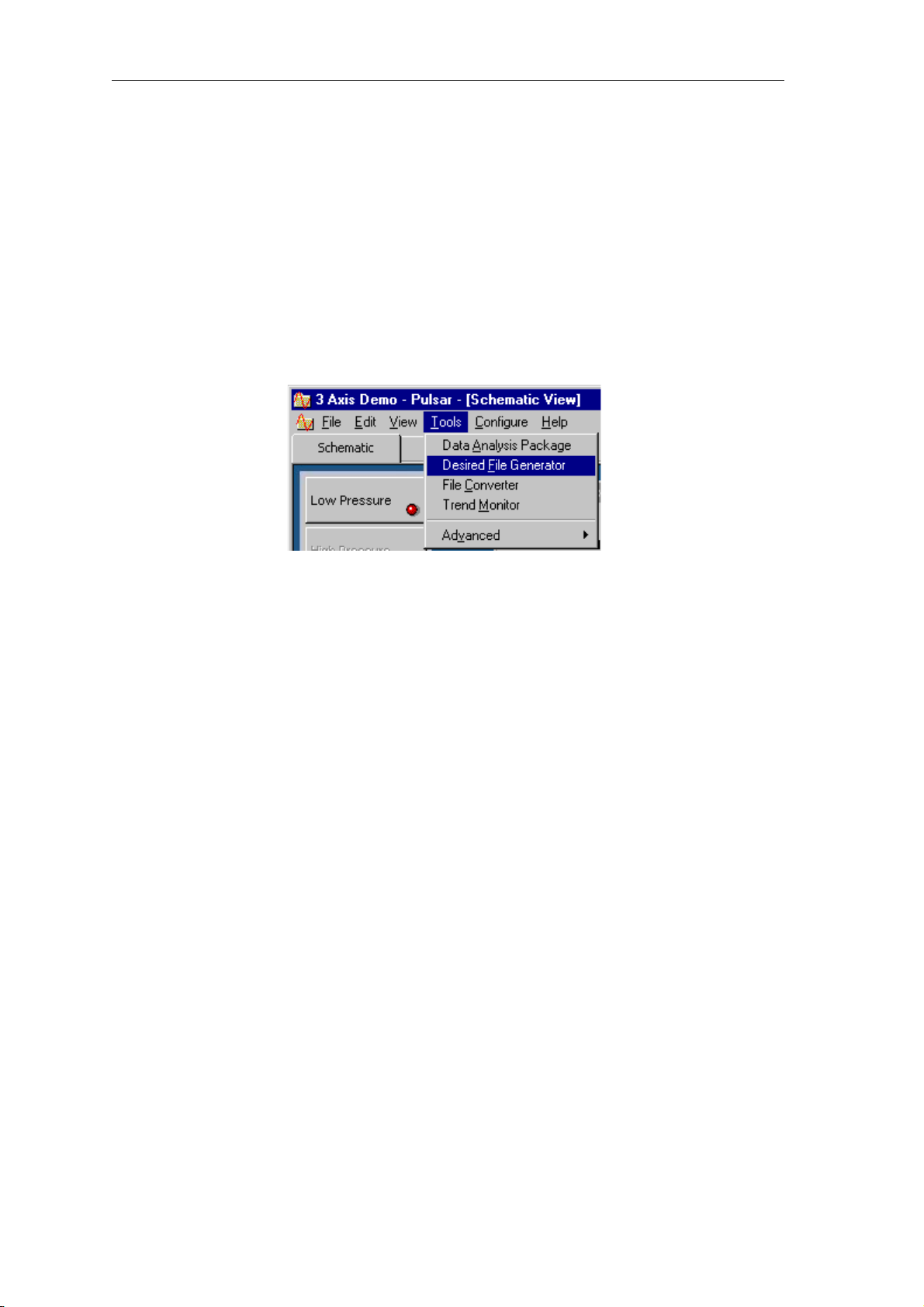
DAP is launched by selecting Data Analysis Package from Pulsar’s
Tools menu.
1.2 The DAP Main Menu.
The DAP menu offers three options:
• Open Data
File button selects a data file to examine.
• Close
Matlab figures closes all Matlab figures except DAP.
• Open Data
File opens a previously saved Dap figure.
Figure 1-2, Main menu
Clicking this button on the Main Menu
will prompt the Select Data Logging File dialogue box. Click on the
required file then OK.
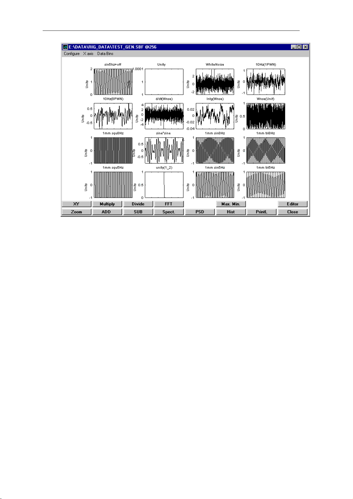
The channels of the selected file will be displayed within the Main
Plot Window. The title of the window is the path and name of the
file being analysed followed by the sample rate of the data.
Up to sixteen plots can be displayed with the title of each plot being
the individual channel name and the y-axis label displaying the units.
1
Figure 1-1, Launching DAP from Pulsar’s Tools menu
Figure 1-3, File
Page 11
General
Valid mat files can also be opened. They should contain the following
variables, in the specified format:
Variable Size Type Comments
loggingrate 1x1 double array
matrix NsxNc double array (matrix of data)
names Ncx20 char array (channel names)
scales Ncx1 double array
units Ncx10 char array
where Ns and Nc represent the number of samples and the number of
channels respectively.
2
Figure 1-4, Main display window
Page 12

General
2. General
The analysis package presents either single or multiple plots whose
data can be analysed or manipulated from selecting options from
either pull-down menus (abbreviated by ⊇) at the top of the figures or
a button bar ([ ]) along the bottom. This manual details each pulldown option and button bar to describe all the features in the Data
Analysis Package.
3
Page 13
Button Bars
3. Pull Down Menus(⊇)
3.1 Main Plot Window - Pull Down Menus
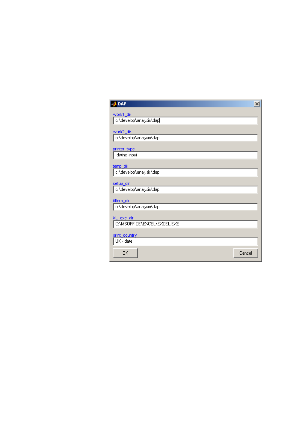
3.1.1 Configure ⊇ Directories
Selecting this option displays the Directories Configuration edit box.
Each of the strings in the boxes can be edited to reflect user
preferences or current PC configuration.
The fields can be edited by highlighting with the mouse. Once edited
if OK is selected the software checks that all the directories specified
do exist and saves the configuration data. If all paths are valid then
the console window displays:
CHECK FINISHED.
1
Figure 3-5, Directories Configuration Edit Box
Page 14

Button Bars
Variable Definitions
work1_dir is the start directory when Select File dialogue boxes are
opened. It corresponds to the directory containing the
file open by Dap.
printer_type configures the printer for all Print commands
-dwinc Send figure to currently installed printer in colour
-noui Buttons are not printed
print_country either UK or US - controls either A4 (UK) or
Letter(US) paper sizes add -date to print the date
and time in the bottom right corner of each plot.
2
Page 15
Button Bars
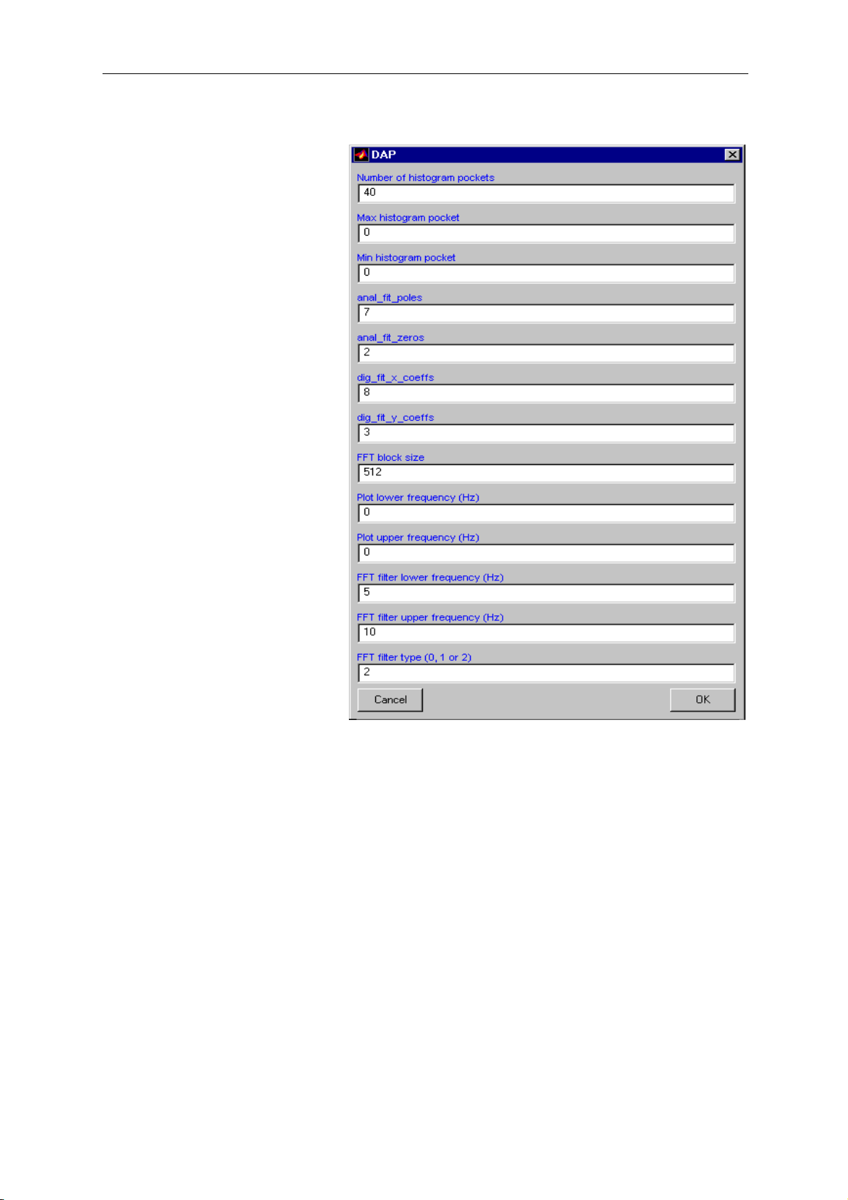
3.1.2 Configure ⊇ Global Data
Figure 3-6, Global Data Config.
Selecting this option pops up the Global Data Configuration Window.
Global Data buttons
Number of histogram pockets See: Button - [Hist]
Max histogram pocket See: Button - [Hist]
Min histogram pocket See: Button - [Hist]
anal_fit_poles See: Button - [An-Fit]
anal_fit_zeros See: Button - [An-Fit]
dig_fit_x_coeffs See: Button - [Dig-Fit]
dig_fit_y_coeffs See: Button - [Dig-Fit]
FFT block size See: Button- [Transf.Funct.]
3
Page 16

Button Bars
Plot lower frequency (Hz) See: Button- [Transf.Funct.]
Plot upper frequency (Hz) See: Button- [Transf.Funct.]
FFT filter lower frequency (Hz) See: Button - [Filt-FFT]
FFT filter upper frequency (Hz) See: Button - [Filt-FFT]
FFT filter type (0, 1 or 2) See: Button - [Filt-FFT]
3.1.3 X axis ⊇ Save as X axis
The mouse pointer will change to cross hairs. The left mouse button
must now be clicked over a selected plot in the Main Plot window.
All subsequent ZOOM plots will now use that data on the X-axis.
3.1.4 X axis ⊇ Time as X axis
This selects ‘time’ in seconds as being the X-axis for all zoom plots.
3.1.5 X axis ⊇ Reset X limits
The x-axis plot range can be modified from within a Zoom window
so that all plots automatically zoom to a selected range of the data
(see X axis ⊇ Set X lims), this option defaults back to the default of
plotting the full channel data when a new Zoom window is selected.
3.1.6 Data Bins ⊇ Save to Bin ⊇S1/S2/S3/S4/S5/S6/S7/S8
Temporary storage bins exist primarily for overplotting data. Channel
data can be stored and retrieved from these bins.
Firstly one of the bins must be selected. The mouse pointer changes
to a cross hair and the left mouse button used to select a channel of
data to store to that bin. The DAP Console window will inform the
operator of the bin that has been selected and the data that has been
stored to it.
3.1.7 Data Bins ⊇ Bin details
This menu option lists the channel names of the data that is currently
stored in the temporary bins. As channel names are not recalled on
overplotted data this can ensure that the correct bin data is to be
retrieved.
3.1.8 Data Bins ⊇ Save Figure
Allows the current figure to be saved as a Matlab file. A new name
must be selected every time this option is activated. This option is
available in all Dap windows as a Data Bins sub-menu or a button.
The figure files thus created can subsequently be open via the Open
figure file button of the main Dap window.
4
Page 17
Button Bars
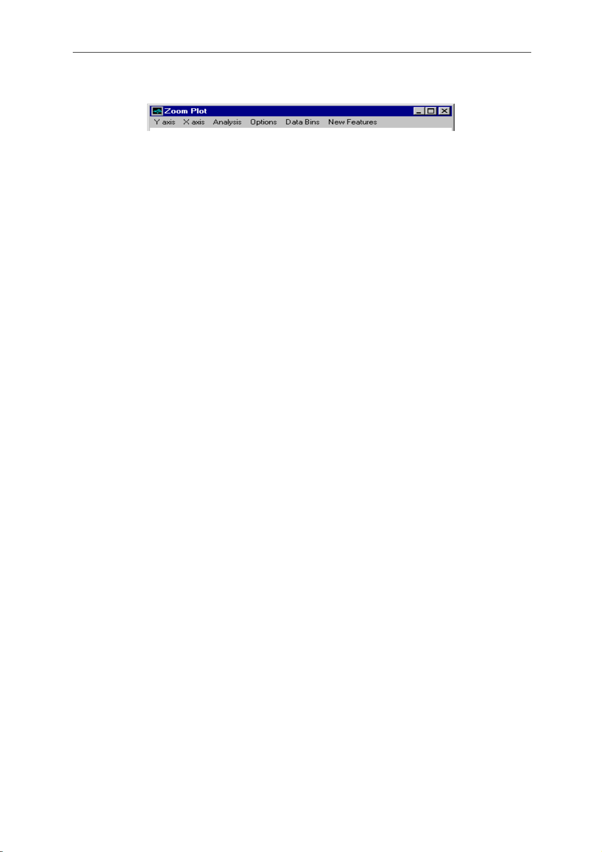
3.2 Zoom windows - Pull Down Menus
This section describes the pull-down menus that can exist in any or
all of the single-plot time domain ‘Zoom’ windows. These include
those entered with the buttons [Zoom], [XY], [Multiply], [Divide],
[ADD], [SUB] and [Hist] from the Main Plot window
3.2.1 Y axis ⊇d/dt
The Y-axis will be differentiated with respect to time. The Y axis
label will be post-scripted with “/sec”.
3.2.2 Y axis ⊇Integr.
The command window will prompt for a start point for the
integration:
Enter the start integration value...
Enter a value the RETURN and the Y-axis will be integrated with
respect to time. The axis label will be post-scripted with “*sec”.
3.2.3 Y axis ⊇Remove Mean
The mean of the data will be removed and the data will be replotted.
The Y axis label will be pre-scripted with “DETREND”.
3.2.4 Y axis ⊇Mean_RMS
The Mean and RMS of the last plot will be printed just below the Xaxis.
3.2.5 Y axis ⊇ABS(Y)
The absolute values of the data will be plotted. The Y axis label will
be pre-scripted with “ABS”.
3.2.6 Y axis ⊇Normalise
The Y axis data is plotted normalised to +1 and -1. The Y axis label
will be pre-scripted with “NORM”.
This function is useful for overplotting data of very different scales.
3.2.7 Y axis ⊇log/lin(y)
The Y-axis will be toggled between linear and logarithmic scales on
consecutive selections of this option.
5
Figure 3-7, Zoom window Pull Down Menus
Page 18
Button Bars
3.2.8 X axis⊇d/dt
The X-axis will be differentiated with respect to time. The X axis
label will be post-scripted with “/sec”.
3.2.9 X axis ⊇Integr.
The command window will prompt for a start point for the
integration:
Enter the start integration value...
Enter a value the RETURN and the X-axis will be integrated with
respect to time. The axis label will be post-scripted with “*sec”.
3.2.10 X axis ⊇Remove Mean
The mean of the data will be removed and the data will be replotted.
The X axis label will be pre-scripted with “DETREND”.
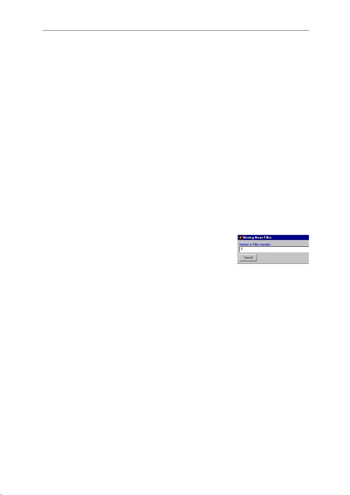
3.2.11 X axis ⊇Filter
Selecting this option pops up the Moving Mean Filter dialogue box. A
zero-phase moving-mean filter will be applied for the number of filter
samples selected.
Five is the default, which essentially
means that each data point is replaced with
the mean of the current point, two points
ahead and two points behind.
The filter strength can be adjusted by
highlighting the five with the mouse and typing a new value. Then
select OK.
3.2.12 X axis ⊇Set X lims
It is possible to rescale the X limits of a Zoom plot. (see Button [Rescale] and Button - [Zoom In]). If the X axis range is of
continued interest then selecting this option means that all subsequent
Zoom plots from the Main Plot window will also be scaled to the
same X axis range. This range selection can be cancelled from the
Main Plot window with X axis ⊇ Reset X limits.
3.2.13 X axis ⊇Get X lims
If X axis ⊇Set X lims is set from a Zoom window and the same x-
axis range is required on an adjacent (already open Zoom window),
then, selecting X axis ⊇Get X lims forces the plot to the new X axis
range.
6
Filter dialogue box
Figure 3-8, Moving Mean
Page 19

Button Bars
3.2.14 X axis ⊇Set Mark
The mouse pointer will become a cross hair and the DAP Console
window will prompt:
Select the X-axis point to draw a line at.
A red vertical line will be placed at the selected point and location of
this “mark” recorded. This is usually to point at the start or end of a
particular event on the data. (See next section X axis ⊇Get Mark)
3.2.15 X axis ⊇Get Mark
The location of the last “mark” set is transferred onto the current plot
with a similar vertical red line.
3.2.16 X axis ⊇Save to X axis
The current Y-axis data will be used as the X-axis for all subsequent
Zoom plots.
The X-axis can be reverted back to being time with X axis ⊇ Time as
X axis from the Main Plot window.
3.2.17 Analysis⊇Curve Fit⊇Linear/Second Order/ Third Order .. etc.
A polynomial fit will be applied to the last Y-axis data plotted in the
Zoom window and the polynomial function overlaid. The polynomial
coefficients and intercept will be printed just below the X-axis.
3.2.18 Analysis⊇Curve Fit⊇Gradient Fit
The mouse pointer will change to cross hairs and the DAP Console
window will assist to prompt for two points on the current Zoom
window. When the two points are selected a line will be draw
between the two pints and the Gradient and Intercept of the line
printed just below the X-axis.
3.2.19 Analysis⊇Spectral⊇Spect(y/x)
Opens the Spectral Window (see section Frequency Domain
Window - Spectral) and displays the Magnitude, Phase and
Coherence between of (Y-axis data)/(X-axis data).
3.2.20 Analysis⊇Spectral⊇PSD
Opens the PSD Window (see section Frequency Domain Window PSD) and displays the PSD of the data in the Y-axis.
3.2.21 Analysis⊇Spectral⊇FRS
This option computes the Frequency Response Spectrum of a time
history (only meaningful for accelerations). The user is prompted for
the damping factor to be used and DAP displays the FRS in a new
7
Page 20
Button Bars
window whose frequency points (x-axis) are defined by the
loggingrate and the current FFT block size. It is then possible to
superimpose the Required Response Spectrum (RRS) used to
generate the time history. The RRS must have been defined in
Desired File Generator (DFG) and the DFG configuration file (*.fcf)
must be available.
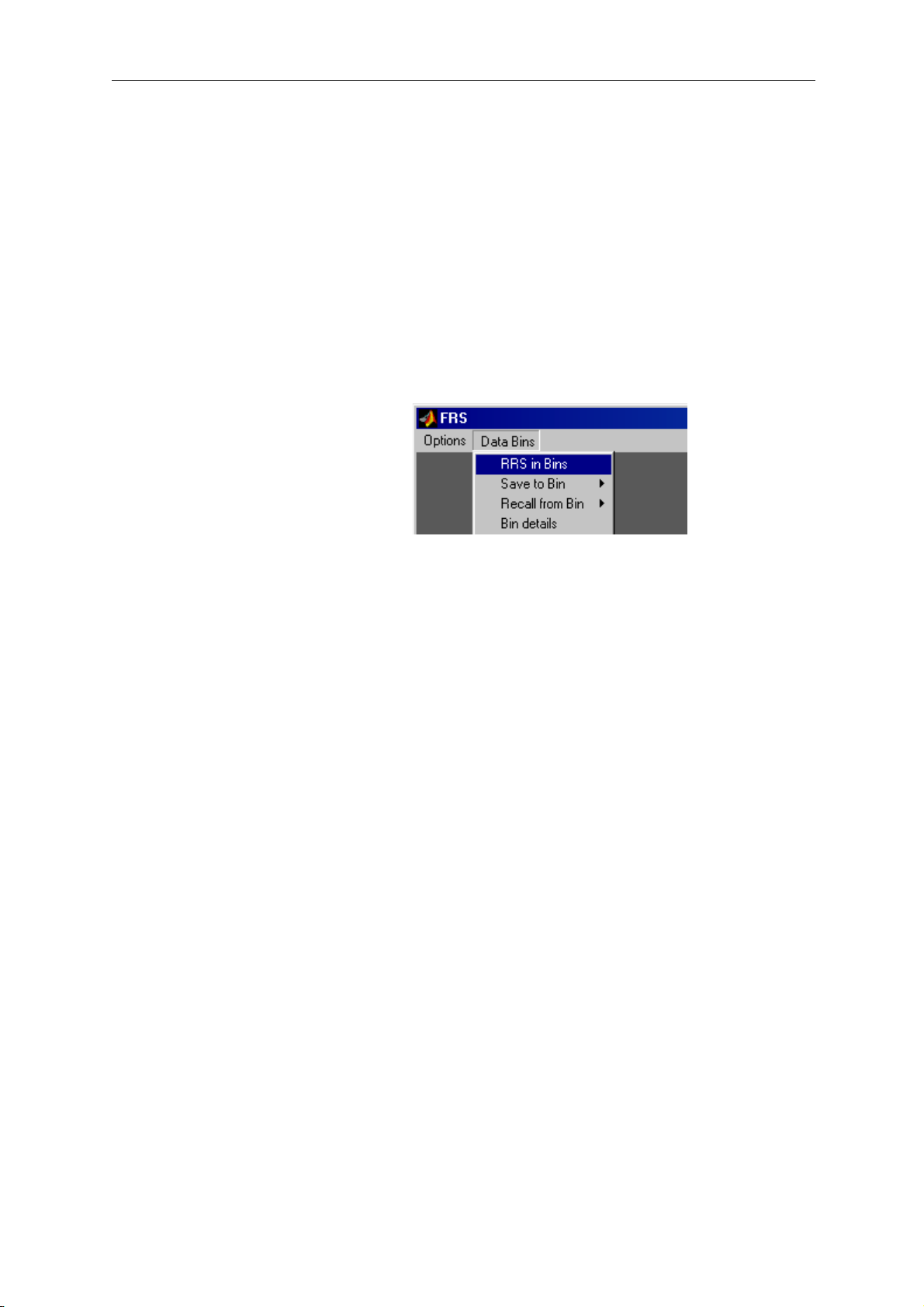
From the Data Bins menu, choose RRS in Bins and select the
appropriate .fcf file. This will store all RRS defined in this file into
the data bins. You can press Bin Details to check that this has been
done.
Then select Recall from Bin to display the required RRS on top of the
current FRS.
3.2.22 Analysis⊇Edit⊇Move Pts
Select this option and the individual data points are highlighted with
blue circles. Click the left mouse button to select a data point, move
to a new position and click again. The blue circle remains where it
was but the plot moves to the new point. Repeat the process for as
many points as required.
Terminate the operation with a right mouse click.
3.2.23 Analysis⊇Edit⊇Smooth Pts
Click the mouse at the start and end data points to smooth with a 1cosine taper.
The DAP Console window will assist with the prompts:
Zoom OFF
Click mouse on START point to SMOOTH..(Right mouse button
to exit)
Click mouse on END point to SMOOTH..(Right mouse button to
exit)
Zoom back ON
3.2.24 Analysis⊇Edit⊇/*+-
The command window prompts:
8
Page 21
Button Bars
Enter Mathematical operator [* / + -] AND value. (I.e. -10):
Type the necessary expression (i.e. type: /100 to reduce the data by a
factor of 100) and return to execute the command.
WARNING: Enclose negative number is parentheses, i.e. /(-1)
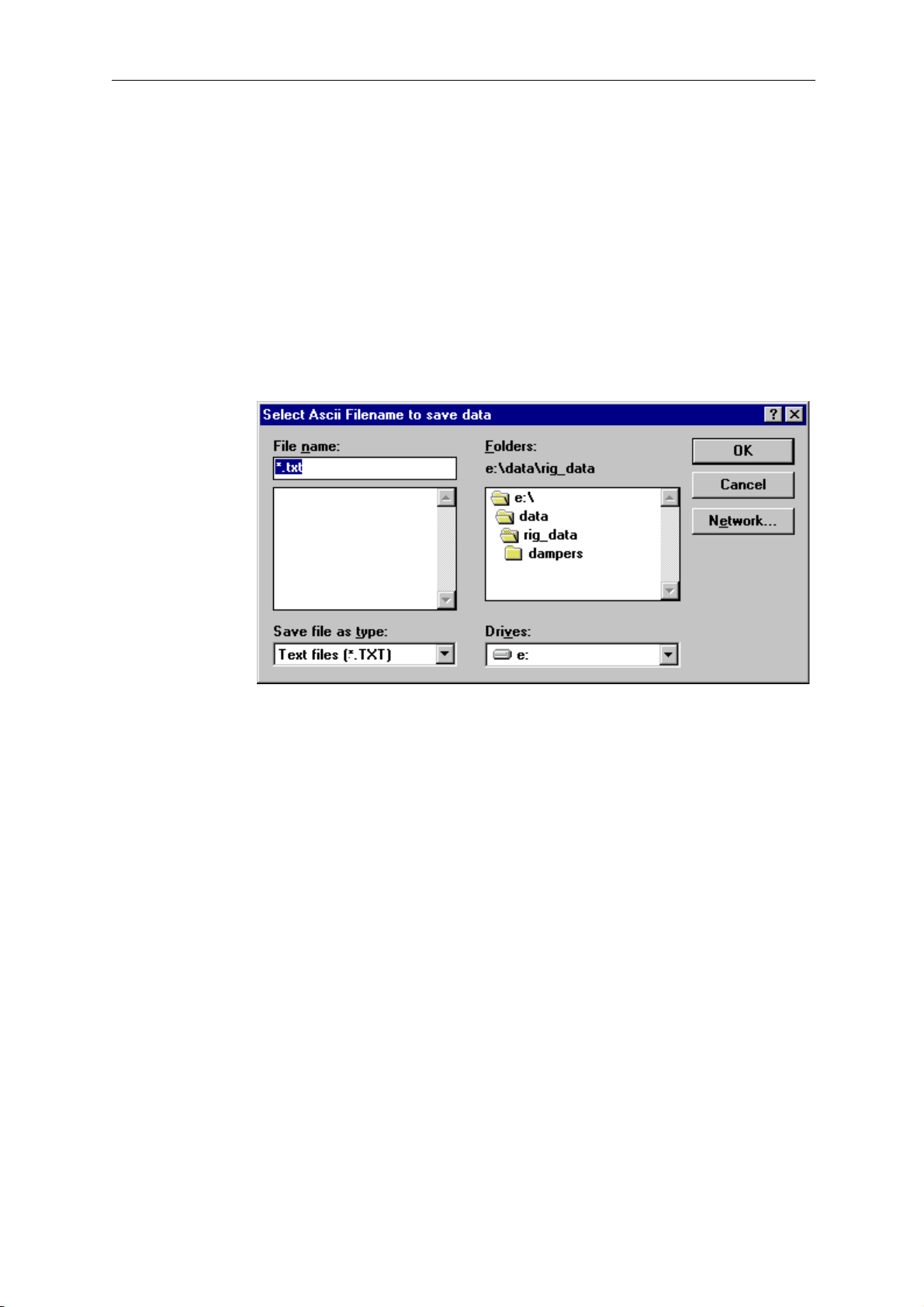
3.2.25 Analysis⊇Save as ASCII
The Save as ASCII dialogue box will appear to prompt for a
filename and directory to save the Y axis data to.
9
Figure 3-9, Save as ASCII dialogue box
Page 22
Button Bars
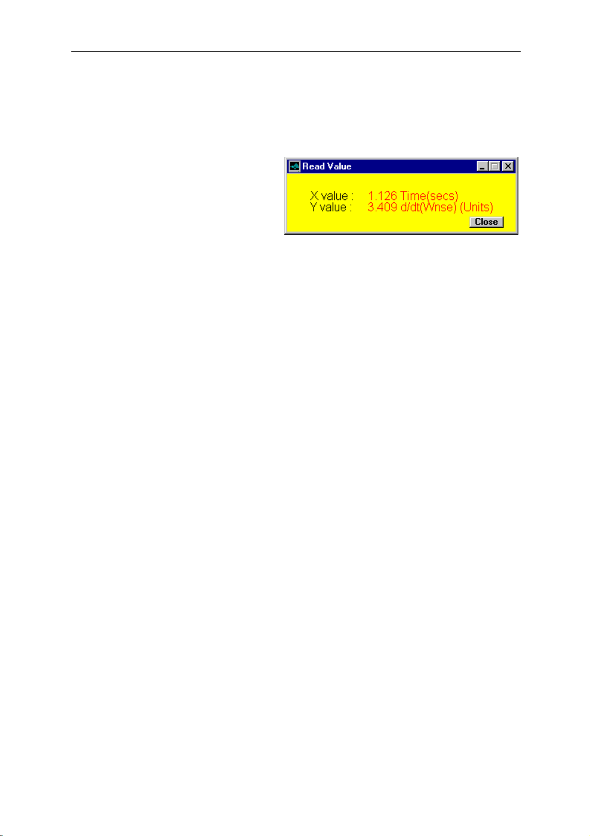
3.2.26 Analysis⊇Read Values
The mouse pointer will change to a cross hair. If it is positioned on
the plot and clicked a dialogue box will appear with those coordinates of that point.
3.2.27 Options⊇Clear plots
All but the last plot in the current Zoom window is removed.
3.2.28 Options⊇Place text
The mouse pointer changes to a cross hair for a point on the plot to be
selected. The DAP Console window prompts the user for the text to
be placed at the selected point.
3.2.29 Options⊇Place date
The mouse pointer changes to a cross hair and a point on the plot
must be selected. Today’s date will be placed starting at that point.
3.2.30 Options⊇Edit Text⊇Title/Ylabel/Xlabel
The Title, Y label or X label of the Zoom window can be changed in
the by typing the required text in the DAP Console window as
prompted.
3.2.31 Options⊇Plot as *s
All the points of the current data will be replaced by *’s. This
function can take a few seconds to overplot the data.
3.2.32 Options⊇Comet Plot
A separate comet plot will be done of the last data plotted in the
current Zoom window. This is useful to show the course of events in
the data - especially for XY plotted data.
1
Figure 3-10, Read Values Dialogue box
Page 23
Button Bars
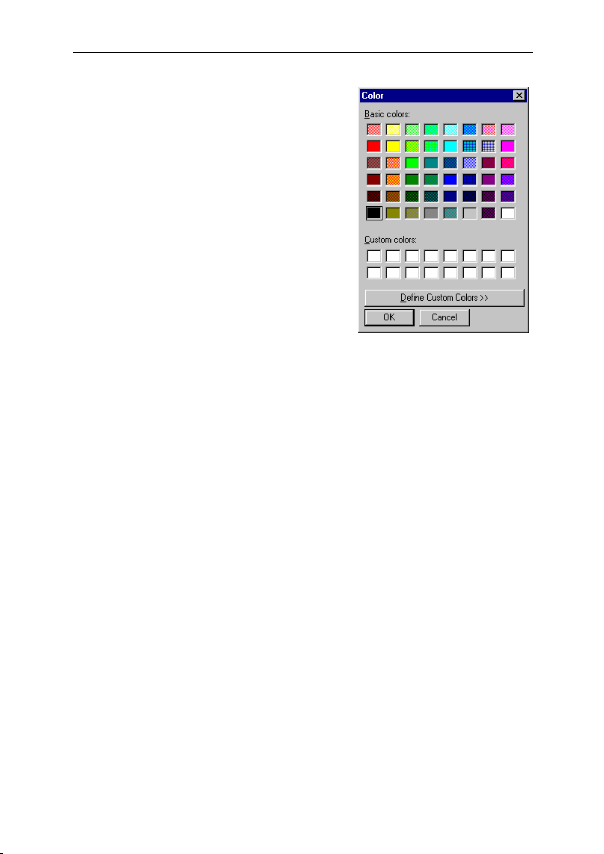
3.2.33 Options⊇Colour
The Colour palette is displayed
to allow the colour of the last
plot to be changed.
3.2.34 Options⊇Turn Grid On
Toggles the Grid ON/OFF in the
current Zoom window.
3.2.35 Options⊇Zoom FULL Out
The plot will zoom full out to
show all the data in the plot.
(I.e. full Y range and X range).
3.2.36 Data Bins⊇ Save to Bin ⊇S1/S2/S3/S4/S5/S6/S7/S8
Temporary storage bins exist primarily for overplotting data. Channel
data can be stored and retrieved from these bins.
This option puts the last plotted data (y-axis data/x axis data/y axis
label and title) in to the required temporary storage bin. The storage is
to hard disk, so can be recovered after a computer power down. The
DAP Console window will inform the operator of the bin that has
been selected and the data that is stored to it.
3.2.37 Data Bins⊇ Recall from Bin ⊇R1/R2/R3/R4/R5/R6/R7/R8
Data can be recalled from any of the storage bins to overplot in the
current Zoom window by selecting the required bin.
3.2.38 Data Bins ⊇ Bin details
This menu options lists channel names of the data that is currently
stored in the temporary bins. As channel names are not recalled on
overplotted data this can ensure that the correct bin data is retrieved.
3.2.39 Data Bins ⊇ Save Figure
Allows the current figure to be saved as a Matlab file. A new name
must be selected every time this option is activated. This option is
available in all Dap windows as a Data Bins sub-menu or a button.
The figure files thus created can subsequently be open via the Open
figure file button of the main Dap window.
1
Figure 3-11, Colour Palette
Page 24
Button Bars
4. Button Bars
4.1 Button Bars - Main Plot window
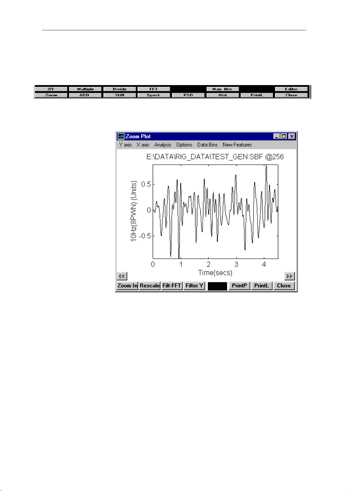
4.1.1 Button - [Zoom]
The format of a time response Zoom window is shown below.
Figure 4-13 Zoom window
The default x-axis is time(seconds) but this can be adjusted with
either Xaxis⊇Save as X axis (from the Main Plot Window) or
Xaxis⊇Save to X axis (from a Zoom window).
The default x range is the full data in the channel, but this can be
adjusted with Xaxis⊇Set X lims and reset with Xaxis⊇Reset X lims.
For full button and pull-down menu operation see the sections
Zoom windows - Button Bars and
Zoom windows - Pull Down Menus.
1
Figure 4-12, Button Bars - Main Plot window
Page 25

Button Bars
4.1.2 Button - [ADD]
There are two prompts in the DAP Console window to select the
required plots in the Main Plot window with a mouse click:
Enter the first value to add...
Enter the second value to add...
A Zoom plot is produced with all the functionality described in the
section Button - [ZOOM]
See sections Zoom windows - Button Bars and Zoom windows -
Pull Down Menus.
4.1.3 Button - [SUB]
There are two prompts in the DAP Console window to select the
required plots in the Main Plot window with a mouse click:
Enter the first value...
Enter the second value to subtract...
A zoom plot is produced with all the functionality described in the
section Button - [ZOOM]
See sections Zoom windows - Button Bars and Zoom windows -
Pull Down Menus.
4.1.4 Button - [Transf.Funct.]
There are two prompts in the DAP Console window to select the
required plots in the Main Plot window with a mouse click:
Click on the OUTPUT signal....
Click on the INPUT signal....
A Spectral Analysis plot is produced in the Frequency domain.
See Section Frequency Domain Window - Spectral for further
details.
4.1.5 Button - [PSD]
There is a prompt in the DAP Console window to select the required
plot with a mouse click.
Click on plot to PSD....
A Power Spectral Density plot is produced in the Frequency domain
See Section Frequency Domain Window - PSD for further details.
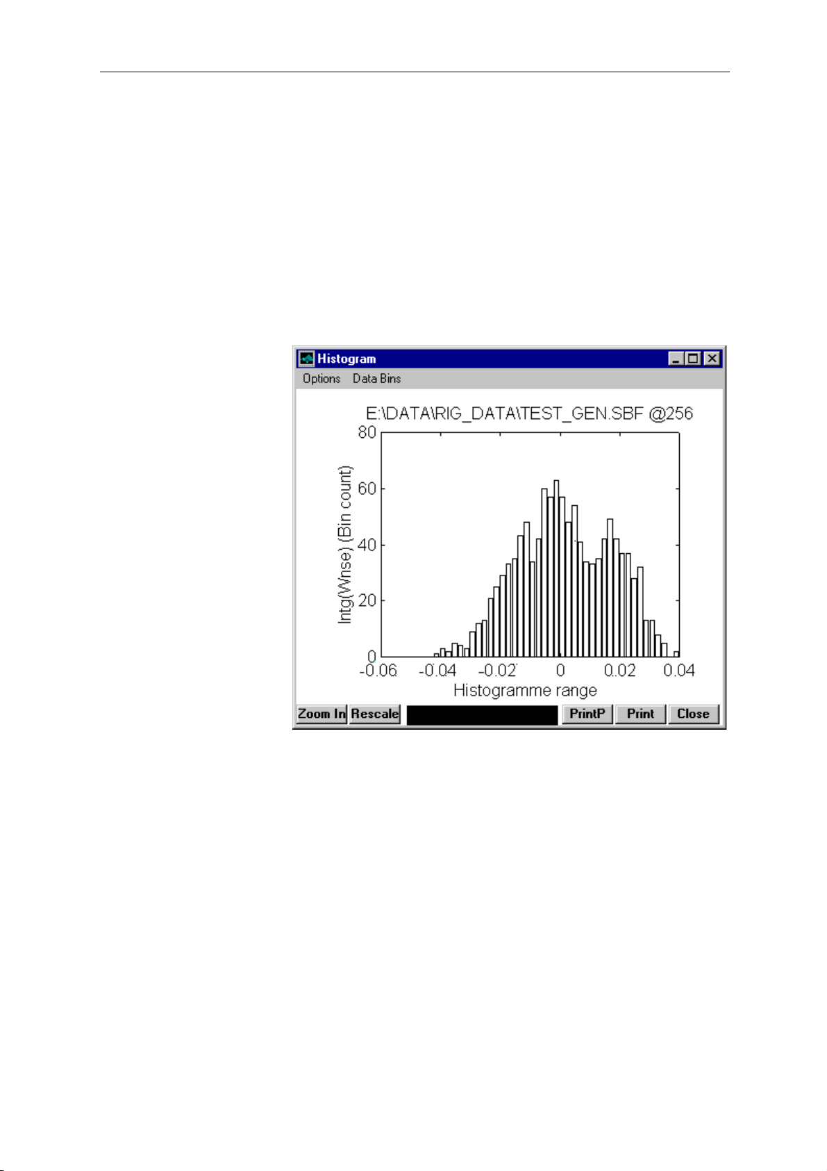
4.1.6 Button - [Hist]
There is a prompt in the DAP Console window to select the required
plot with a mouse click.
Click on plot to Histogramate....
1
Page 26
Button Bars
A histogramme plot is produced of the selected data.
The Pockets are controlled by the variables
hist_pockets number of histogramme pockets (bins)
hist_max max. value to histogrammate to
hist_min min. value to histogrammate to
If hist_max and hist_min are zero all the data used to populate the
bins.
set from Global Data in the Main Menu
See sections Zoom windows - Button Bars and Zoom windows -
Pull Down Menus.
4.1.7 Button - [PrintL]
Clicking on the PrintL button sends the current Main Plot window to
the current windows printer and will be plotted in LANDSCAPE.
See also Configure⊇Directories especially printer_type and
printer_country
4.1.8 Button - [Close]
Closes the Main Plot window
1
Figure 4-14, Histogramme Plot
Page 27

Button Bars
4.1.9 Button - [XY]
There are two prompts in the DAP Console window to select the
required plots in the Main Plot window with a mouse click :
Enter Y axis...
Enter X axis...
A Zoom plot is produced with all the functionality described in the
section Button - [ZOOM]
See sections Zoom windows - Button Bars and Zoom windows -
Pull Down Menus.
4.1.10 Button - [Multiply]
There are two prompts in the DAP Console window to select the
required plots in the Main Plot window with a mouse click :
Click with mouse on first multiplicator ....
Click with mouse on second ....
A Zoom plot is produced with all the functionality described in the
section Button - [ZOOM]
See sections Zoom windows - Button Bars and Zoom windows -
Pull Down Menus.
4.1.11 Button - [Divide]
There are two prompts in the DAP Console window to select the
required plots in the Main Plot window with a mouse click :
Click with mouse on Numerator....
Click with mouse on Denominator....
A Zoom plot is produced with all the functionality described in the
section Button - [ZOOM]
See sections Zoom windows - Button Bars and Zoom windows -
Pull Down Menus.
4.1.12 Button - [FFT]
There is a prompt in the DAP Console window to select the required
plot with a mouse click.
Click on plot to FFT on....
A FFT Analysis plot is produced.
See Section Frequency Domain Window - FFT for further details
1
Page 28
Button Bars
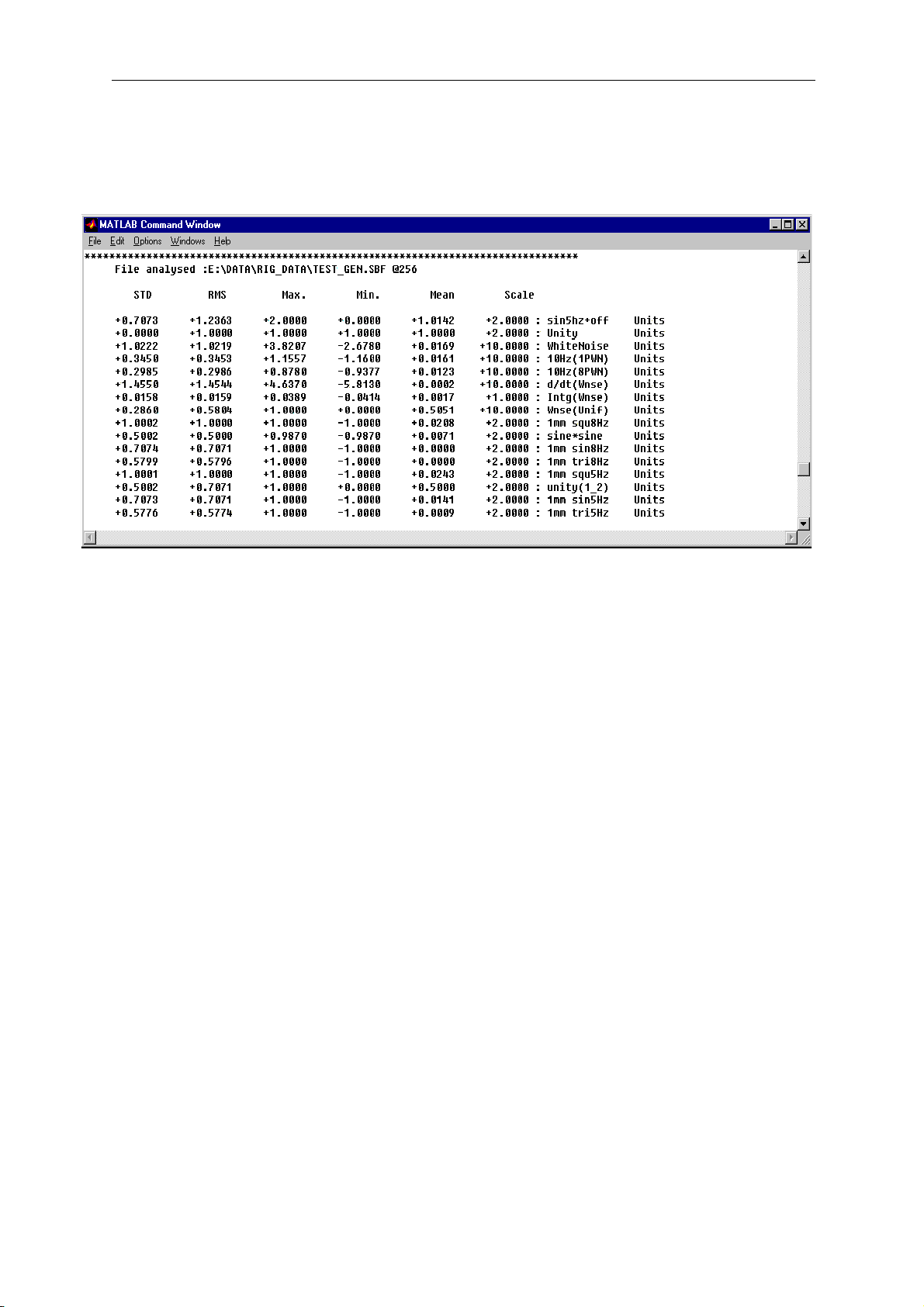
4.1.13 Button - [Max. Min.]
When this button is clicked the Standard Deviation, RMS, Maximum
value, Minimum value, Mean and the Scale value of every channel in
the Main Plot window is recorded in the DAP Console window.
4.1.14 Button - [Editor]
The button toggles in and out of Editor Mode
When the button is first clicked the Main Plot window enters Edit
Mode. The Background will turn blue to indicate this. Clicking the
button again returns to normal Data Analysis Mode.
Additional Pull down menus are available in Edit mode to allow
editing of the channels.
See section Edit Mode if this button is available.
4.2 Zoom windows - Button Bars
4.2.1 Button - [Zoom In]
Clicking on the Zoom In button turns on the grid on for the plot. It is
now possible to adjust a rubber band box to zoom in on a selected
area. Click the left mouse button on the plot. Hold down the mouse
button and stretch the ‘rubber-band’ box that appears over the
required zoom area. Release the mouse when the required area is
covered. The plot will then displays the new zoom area. This process
can be repeated time and time again.
Clicking the right mouse button zooms out to the last zoom area.
Double clicking the right mouse button does a maximum zoom out.
1
Figure 4-15, Display STD, RMS., Max., Min., Mean and Scale values.
Page 29
Button Bars
4.2.2 Button - [Rescale]
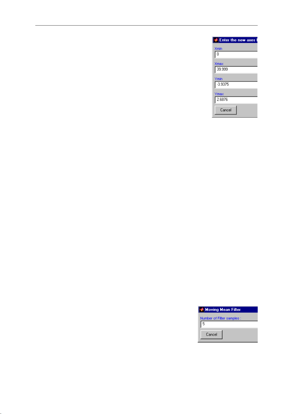
Clicking on the Rescale button pops up the
rescale box. The current axis maximum and
minimum scales are displayed. Use the mouse to
highlight and edit any of the values then select
OK. The Zoom plot is adjusted to the new axes.
4.2.3 Button - [FFT-Filt]
Clicking on the FFT-Filt button causes a zerophase brick-wall band-pass filter to be applied to
the data in the current Zoom window. The upper
and lower frequencies of the band pass are
specified from the Global Data menu (as
fft_filt_min and fft_filt_max).
If fft_all1_frame0 is set to 0 a time domain Butterworth (zero phase)
filter is applied to the data. The DAP Console window informs of the
progress.
Filter applied to LAST plot.(includes curve fits and
Overplots)
Butterworth Order = xx
If the filter cannot be applied then an error message appears in the
DAP Console window.
If fft_all1_frame0 is set to 1 a Yulewalker method of time domain
filtering is applied.
If the filter cannot be applied then an error message appears in the
DAP Console window.
If fft_all1_frame0 is set to 2 a frequency domain method is used.
This can only apply a filter to fixed frame sizes of data (specified by
mpnt_spectral in the Global Data menu). The remaining data is
zeroed.
See section Frequency Domain Window - FFT
4.2.4 Button - [Filter Y]
Clicking on the Filter Y button pops up
the Moving Mean Filter dialogue box. A
zero-phase moving-mean filter is applied
for the number of filter samples selected.
Five is the default. This can be edited by
highlighting with the mouse. Then select
either Cancel or OK.
1
dialogue box
dialogue box
Figure 4-16, Rescale
Figure 4-17, Mean Filter
Page 30

Button Bars
4.2.5 Button - [PrintP]
Clicking on the PrintP button sends the current Zoom plot to the
current windows printer and plots in PORTRAIT.
See also the main section: Configure⊇Directories especially
printer_type and print_country
4.2.6 Button - [PrintL]
Clicking on the PrintL button sends the current Zoom plot to the
current windows printer and plots in LANDSCAPE.
See also the main section: Configure⊇Directories especially
printer_type and print_country
4.2.7 Button - [Close]
Clicking on the Close button closes the current Zoom window
4.2.8 Button - [<<] & [>>]
Clicking on the << arrows moves the plot view 25% of the X axis
scale to the left.
Clicking on the >> arrows moves the plot view 25% of the X axis
scale to the right.
1
Page 31
Frequency Domain Windows
5. Frequency Domain Windows
The frequency analysis frame size for all frequency analysis is
controlled by the variable mpnt_spectral set from Global Data in the
Main Menu.
The Frequency is plotted with the maximum and minimum set by
plot_min_freq and plot_min_freq (in Global Data) respectively. If
these are set to zero the plots are auto scaled.
5.1 Frequency Domain Windows - Pull Down Menus (⊇)
5.1.1 Options ⊇log/lin(x)
The X-axis will be toggled between linear and logarithmic scales on
consecutive selections of this option.
5.1.2 Options⊇Gradient Fit
The mouse pointer will change to cross hairs and the DAP Console
window will assist to prompt for two points on the current Zoom
window. When the two points are selected a line will be draw
between the two pints and the Gradient and Intercept of the line
printed just below the X-axis.
5.1.3 Options ⊇log/lin(y)
The Y axis will be toggled between linear and logarithmic scales on
consecutive selections of this option.
5.1.4 Options ⊇dB
The Y axis will be toggled between Linear and Log scales on
consecutive selections of this option.
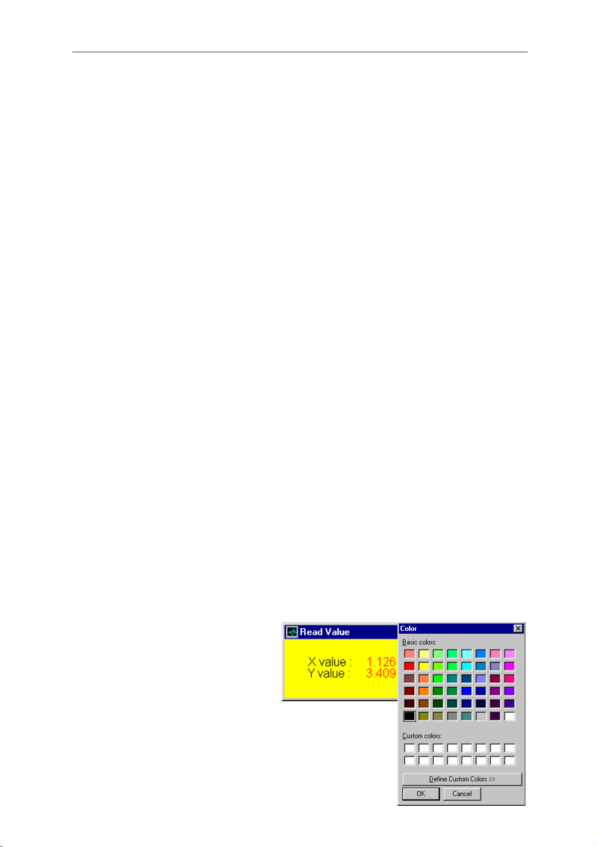
5.1.5 Options⊇Read Values
The mouse pointer will change to a cross hair. If it is positioned on
the plot and clicked a dialogue box will appear with those coordinates.
5.1.6 Options⊇Colour
The Colour palette is displayed to allow
the colour of the last plot to be altered.
1
Figure 5-18, 1 Read Values Dialogue box
Figure 5-19, Colour Palette
Page 32

Frequency Domain Windows
5.1.7 Options⊇Turn Grid On
Toggles the Grid ON/OFF in the current Zoom window.
5.1.8 Options⊇Zoom FULL Out
The plot will be expanded to show all the data in the plot. (i.e. full Y
range and X range).
5.1.9 Data Bins⊇ Save to Bin ⊇S1/S2/S3/S4/S5/S6/S7/S8
Temporary storage bins exist primarily for overplotting data. Channel
data can be stored and retrieved from these bins.
This option puts the last plotted data ( y axis data/x axis data/y axis
label and title) in to the required temporary storage bin. The storage is
to hard disk so can be recovered after a computer power down. The
DAP Console window will inform the operator of the bin that has
been selected and the data that is stored to it.
5.1.10 Data Bins⊇ Recall from Bin ⊇R1/R2/R3/R4/R5/R6/R7/R8
Data can be recalled from any of the storage bins to overplot in the
current Zoom window by selecting the required bin.
5.1.11 Data Bins ⊇ Bin details
This menu options lists channel names of the data that is currently
stored in the temporary bins. As channel names are not recalled on
overplotted data this can ensure that the correct bin data is retrieved.
5.1.12 Data Bins ⊇ Save Figure
Allows the current figure to be saved as a Matlab file. A new name
must be selected every time this option is activated. This option is
available in all Dap windows as a Data Bins sub-menu or a button.
The figure files thus created can subsequently be open via the Open
figure file button of the main Dap window.
5.2 Frequency Domain Windows - Button bars ([ ])
5.2.1 Button - [Zoom In]
Clicking on the Zoom In button turns on the grid on the plot. It is
now possible to adjust a rubber band box to zoom in on a selected
area. Click the left mouse button on the plot. Hold down the mouse
button and stretch the ‘rubber-band’ box that appears over the
required zoom area. Release the mouse when the required area is
2
Page 33
Frequency Domain Windows
covered. The plot will then displays the new zoom area. This process
can be repeated time and time again.
Clicking the right mouse button zooms out to the last zoom area.
Double clicking the right mouse button does a maximum zoom out.
5.2.2 Button - [Rescale]
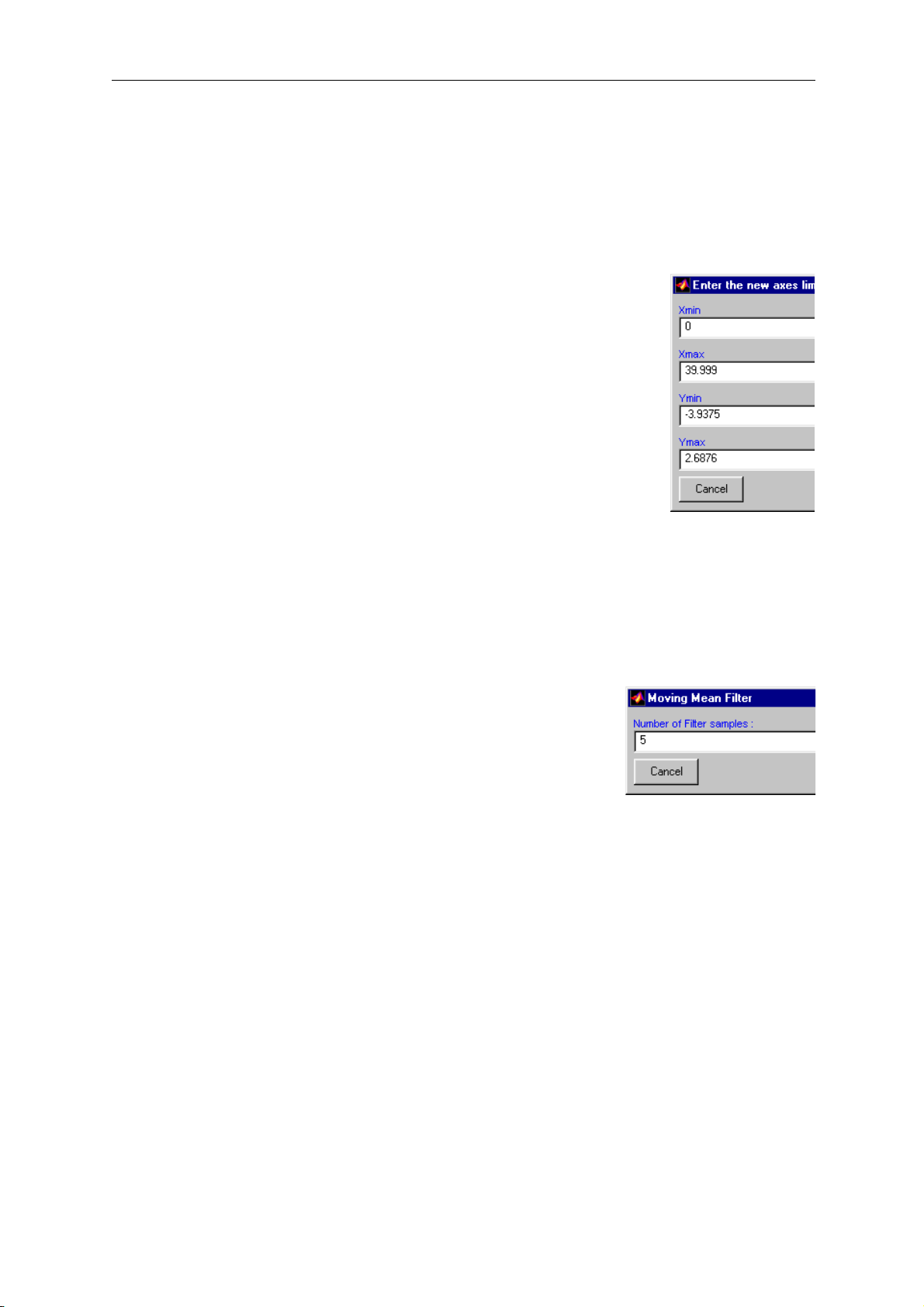
Clicking on the Rescale button pops up the
rescale box. The current axis maximum and
minimum scales are displayed. Use the mouse to
highlight and edit any of the values then select
OK. The Zoom plot is adjusted to the new axes.
5.2.3 Button - [dy/dt]
The data will be differentiated with respect to
time. In the frequency domain this involves
multiplying each point by (2*pi*frequency)
5.2.4 Button - [Integr.]
The data will be integrated with respect to time. In the frequency
domain this involves dividing each point by (2*pi*frequency)
5.2.5 Button - [Filter Y]
Clicking on the Filter Y button pops up the Moving Mean Filter
dialogue box. A zero-phase moving-mean
filter is applied for the number of filter
samples selected. Five is the default. This
can be edited by highlighting with the
mouse. Then select OK. This filter is
applied to the frequency domain points and
should be used if the coherence is poor to
smooth the plot.
WARNING: This filter is applied to the frequency data NOT to the
time domain data that formed it
5.2.6 Button - [Print]
Clicking on the Print button sends the current Zoom plot to the
current windows printer and plots in PORTRAIT.See also the main
section : Configure⊇Directories especially printer_type and
print_country
5.2.7 Button - [Close]
Clicking on the Close button closes the current Zoom window
3
dialogue box
box
Figure 5-20, Rescale
Figure 5-21, Filter dialogue
Page 34

Frequency Domain Windows
5.2.8 Button - [Zoom]
The mouse pointer will change to cross hairs and the DAP Console
window will prompt for a plot to be selected. A Frequency Domain
Plot window will open showing the selected plot with the various data
analysis and display tool available.
See Section Frequency Domain Window - Zoom.
5.2.9 Button - [An_Fit]
See Section Analogue frequency domain fit to data.
5.2.10 Button - [Dig_Fit]
See Section Digital (IIR) frequency domain fit to data
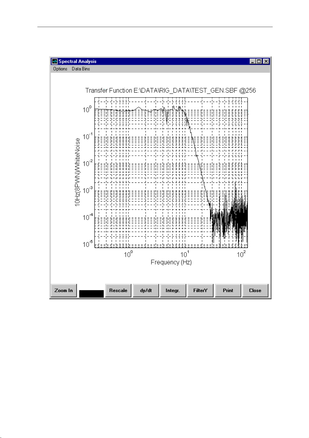
5.3 Frequency Domain Window - Spectral
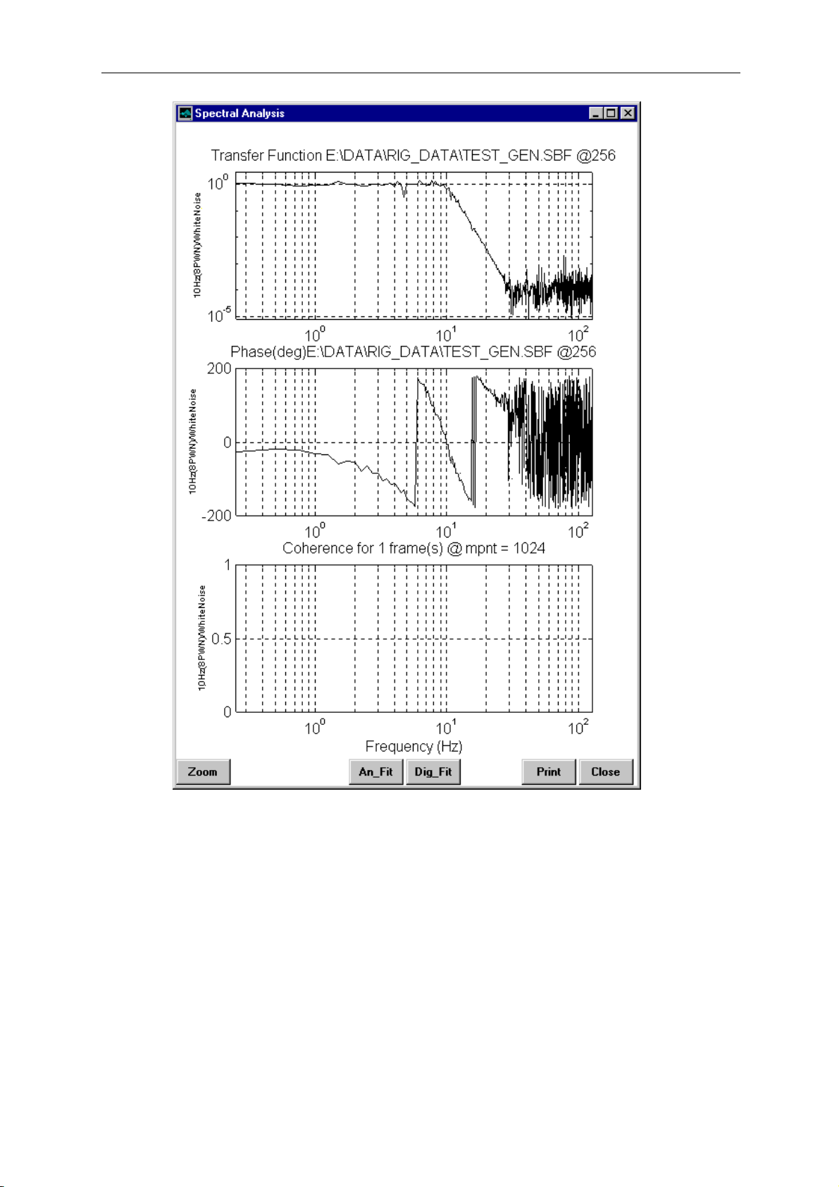
A Spectral Analysis plot can be generated from the Main Plot window
button [Transf.Funct.] or from a Zoom window from the pull down
menu Analysis⊇Spectral⊇Spect(y/x)
Both produce the Spectral Analysis plot which includes:
• Transfer Function of
Output/Input
• Phase between the
Output/Input
• Coherence Plot between the
Output/Input
4
Page 35
Frequency Domain Windows
See also sections:
Frequency Domain Windows - Button Bars sub section
Button - [Zoom]
Analogue Frequency Domain Fit to Data
Digitai (IIR) Frequency Domain Fit to Data
Frequency Domain Windows - Button Bars sub section
Button - [Print]
Frequency Domain Windows - Button Bars sub section Button [Close]
5
Figure 5-22, Spectral Analysis Plot
Page 36
Frequency Domain Windows
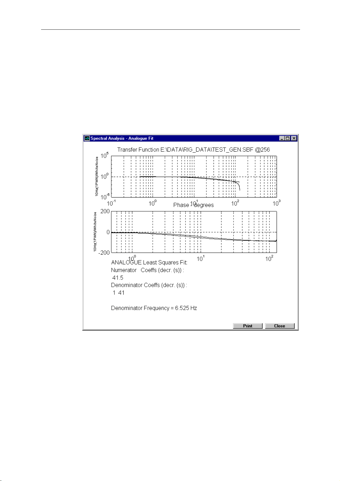
5.4 Analogue frequency domain fit to data
This enables a multiple pole and multiple zeros transfer function to
be “best-fit” to the data. The number of poles and zeros are
determined by anal_fit_poles and anal_fit_zeros in Global Data.
The Spectral Analysis - Analogue Fit window is produced with the
Numerator and Denominator coefficients of the be “best-fit” transfer
function displayed at the base.
If the fit is for a single or two pole system then the natural frequency
(and critical damping for a two pole system) is also printed on the
plot.
See also sections:
Frequency Domain Windows - Button Bars sub section
Button - [Print]
Frequency Domain Windows - Button Bars sub section
Button - [Close]
6
Figure 5-23, Analogue frequency domain fit to data
Page 37
Frequency Domain Windows
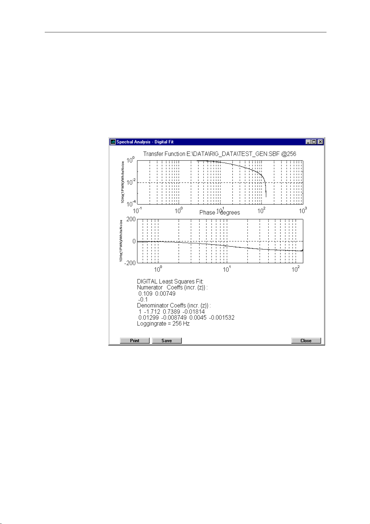
5.5 Digital (IIR) frequency domain fit to data
This enables a “best-fit” IIR filter to be fitted to the data. The number
of recursive and non-recursive coefficients are determined by
dig_fit_x_coeffs and dig_fit_x_coeffs in Global Data.
The Spectral Analysis - Digital Fit window is produced with the
coefficients of the be “best-fit” transfer function displayed at the
base.
These coefficients can be saved to disk in ascii format using the
[Save] button.
See also sections :
Frequency Domain Windows - Button Bars sub section
Button - [Print]
Frequency Domain Windows - Button Bars sub section
Button - [Close]
7
Figure 5-24, Digital (IIR) frequency domain fit to data
Page 38
Frequency Domain Windows
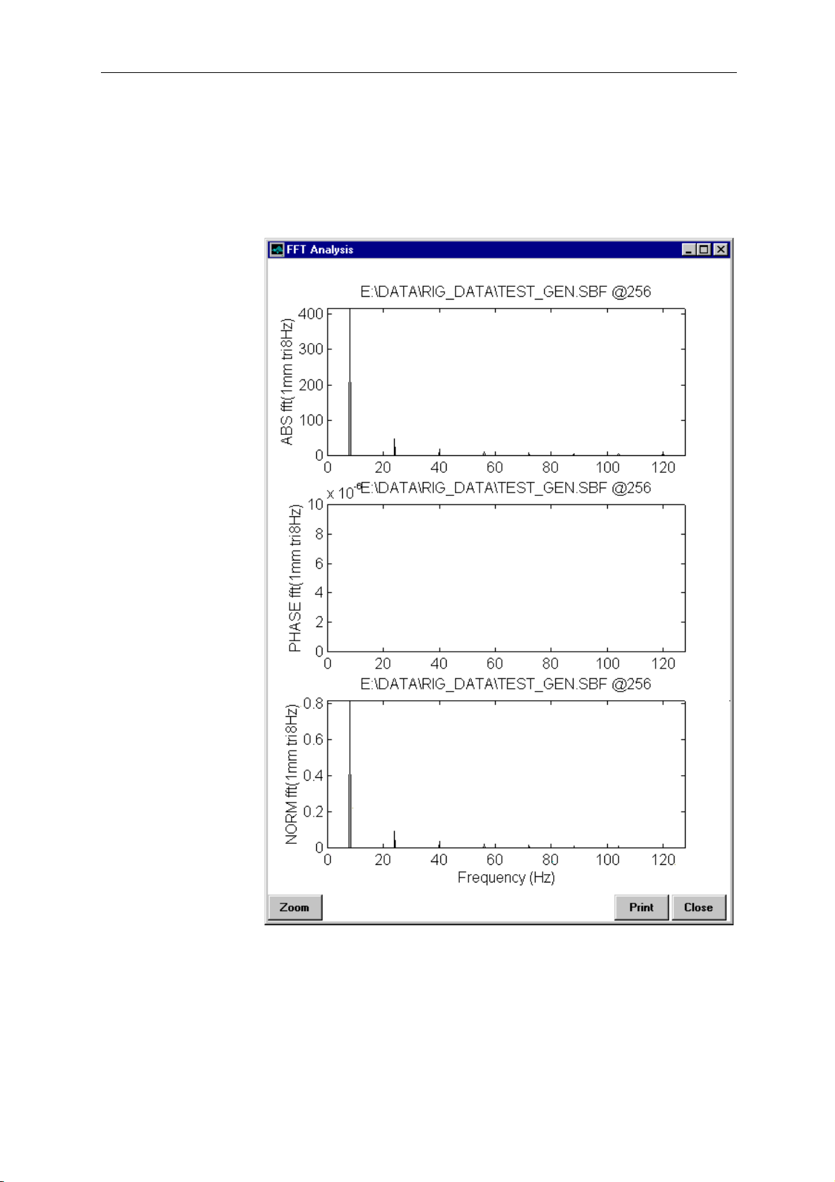
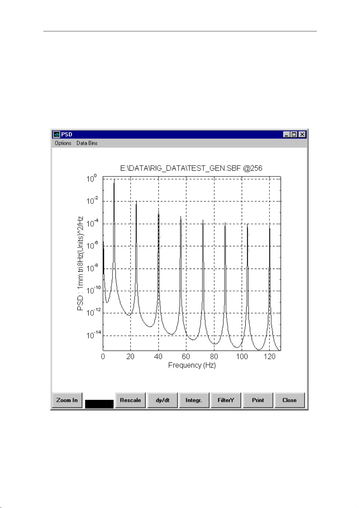
5.6 Frequency Domain Window - FFT
This option is available only from the Main Plot window button
[FFT]. The result is the FFT Analysis plot below of the selected
channel of data.
See also sections :
Frequency Domain Windows - Button Bars sub section
Button - [Zoom]
8
Figure 5-25, Frequency Domain FFT
Page 39
Frequency Domain Windows
Frequency Domain Windows - Button Bars sub section
Button - [Print]
Frequency Domain Windows - Button Bars sub section
Button - [Close]
5.7 Frequency Domain Window - PSD
See Sections
Frequency Domain Windows - Pull Down Menus (⊇) and
Frequency Domain Windows - Button Bars ([ ])
9
Figure 5-26, PSD Plot
Page 40
Frequency Domain Windows
5.8 Frequency Domain Window - Zoom
See Sections
Frequency Domain Windows - Pull Down Menus (⊇) and
Frequency Domain Windows - Button Bars ([ ])
1
Figure 5-27, Frequency Domain Window - Zoom window
Page 41
Edit Mode
6. Edit Mode
Four additional pull-down menus appear when the Edit mode is
enabled :
Edit ONE, Edit ALL, Waveforms and Save File.
Their functionality is described in the following sections.
6.1 Edit Mode - Additional Pull Down Menus (⊇)
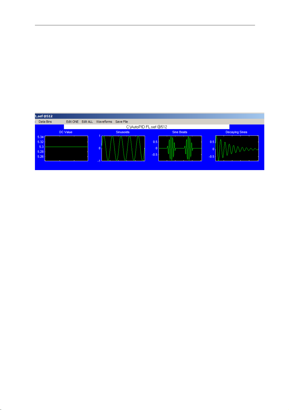
6.1.1 Waveforms
The Waveforms menu allows four types of waveforms to be
generated and saved in the data file. The four types (DC Value,
Sinusoids, Sine Beats and Decaying Sines) are illustrated in Figure 61 above.
6.1.2 Edit ONE⊇/*+-
The mouse pointer will change to a cross hair and the DAP Console
window will prompt :
Click on plot to MODIFY....
Having selected a plot it will further prompt :
Enter Mathematical operator [* / + -] AND value.(i.e. -10) :
Type the necessary expression (i.e. type : /100 to reduce the
data by a factor of 100) and return to execute the command.
WARNINGS:
Enclose negative number is parentheses, i.e. /(-1)
1
Figure 6-28, Edit Mode Pull-Down Menus
Page 42

Edit Mode
Each channel has a scale factor. It defines the maximum and
minimum range of the data so that data can be save as integer format.
If the mathematical operations take the data over the scale factor an
error message will appear .
It is necessary to change the scale factor (Edit ONE⊇Change Scale)
before the operation can be completed.
Equally important - if data is reduced in magnitude and the Scale
factor left large there will be poor resolution when the data is saved to
disk. There is no warning for this but when any files is loaded by
DAP all the channels are checked for poor resolution and, if so, a
warning message is written to the DAP Console window.
Example of the DAP Console window display on opening a file.
File E:\DATA\RIG_DATA\TEST_GEN.SBF is in Version 5 SBF format.
Number of samples in each channel : 1152
WARNING : Data resolution is +0.00 % on channel 2
6.1.3 Edit ONE⊇Start (1-COS)
The mouse pointer will change to a cross hair and the DAP Console
window will prompt :
Click on plot to MODIFY....
Having selected a plot it will further prompt :
Enter START (1-Cosine) duration sec’s.
Enter the duration of the taper and RETURN and it will be applied to
the beginning of the selected channel.
6.1.4 Edit ONE⊇End (1-COS)
The mouse pointer will change to a cross hair and the DAP Console
window will prompt :
Click on plot to MODIFY....
Having selected a plot it will further prompt :
Enter END (1-Cosine) duration sec’s.
Enter the duration of the taper and RETURN and it will be applied to
the end of the selected channel.
6.1.5 Edit ONE⊇Envelope Taper
See section 6.1.19
2
Page 43

Edit Mode
6.1.6 Edit ONE⊇Remove Mean
The mouse pointer will change to a cross hair and the DAP Console
window will prompt :
Click on plot to DETREND....
The mean will be removed from the selected channel.
6.1.7 Edit ONE⊇Edit Text⊇Name(Title)
The mouse pointer will change to a cross hair and the DAP Console
window will prompt :
Click on plot to Edit NAME ....
Having selected a plot it will further prompt :
Original name was xxxxxxx - Enter New NAME :
Type the new name in the Command Window and RETURN will add
the new title to the selected plot.
6.1.8 Edit ONE⊇Edit Text⊇Units(ylabel)
The mouse pointer will change to a cross hair and the DAP Console
window will prompt :
Click on plot to Edit UNITS ....
Having selected a plot it will further prompt :
Original units were xxxx - Enter New UNITS :
Type the new name in the Command Window and RETURN will add
the new y label to the selected plot.
6.1.9 Edit ONE⊇Change Scale
The mouse pointer will change to a cross hair and the DAP Console
window will prompt :
Click on plot to MODIFY Scale on ....
Plot selected : xxxx
Current scale is xx
Enter new Max. and Min. scale value :
Enter the new scale value and RETURN.
To read the scales on all the channels use the button [Max. Min.] in
the Main Command Window.
6.1.10 Edit ONE⊇DELETE
The mouse pointer will change to a cross hair and the DAP Console
window will prompt:
3
Page 44

Edit Mode
Click on plots to DELETE ....(RIGHT MOUSE Button to
EXIT)
As each plot is selected with the mouse it is deleted. To terminate the
operation click the right mouse button.
6.1.11 Edit ONE⊇MOVE
The mouse pointer will change to a cross hair and the DAP Console
window will prompt
Click on plot to MOVE ....(RIGHT MOUSE Button to
EXIT)
Select the plot to move with the mouse, the Command Window will
then prompt :
Click on new position ....
Any of the sixteen plot position can be selected. If the position is
empty the plot is moved otherwise the existing plot discarded and
overwritten.
6.1.12 Edit ONE⊇ADD(BIN)⊇Bin1/2/3/4/5/6/7/8
When a bin is selected the Command Window displays the contents
of the bin :
Duration of plot =xxxx seconds.
Channel xxxxx xxxxx
Max(ABS(data)) = xxxx
and prompts firstly for a scale for the channel (which must be greater
than the Max(ABS(data) value).
Enter Channel scale value
and then for a position to place the data:
Click on new position ....
The bin is placed at that position. If the data has less points than the
existing data channels the data is extended with zeros, if it is longer
then it is truncated.
6.1.13 Edit ALL⊇New Start Time
The DAP Console window will display the current length of the file :
Duration of plot =xxxx seconds.
then prompt for a new start time
Enter START time (secs.)
All the channels will be updated with all the data discarded before
this time.
4
Page 45

Edit Mode
If a negative start time is stated then the data is extended and this
period of time is added to the beginning of all the channels as zeros.
6.1.14 Edit ALL⊇New End Time
The DAP Console window will display the current length of the file :
Duration of plot =xxxx seconds.
then prompt for a new end time
Enter END time (sec’s.)
All the channels will be updated with all data discarded after this
time. If the time is greater than the length of the data then all the
channels are extended (with zeros) up to the new time.
6.1.15 Edit ALL⊇CUT - DISCARD
The DAP Console window will display the current length of the file
Duration of plot =xxx seconds.
and prompt for a start time:
Enter START time of data to DISCARD (sec’s.)
then an end time :
Enter END time of data to DISCARD (sec’s.)
the data between the two times (on all the channels) will be discarded
and all the plots updated and the Command Window will display :
New duration of data is xxx seconds.
6.1.16 Edit ALL⊇Cosine Taper⊇Start
The DAP Console window will prompt :
Duration of plot = xxxx seconds.
Enter START (1-Cosine) duration sec’s.
Enter the duration of the taper and RETURN and it will be applied to
the start of all the channels.
6.1.17 Edit ALL⊇Cosine Taper⊇End
The DAP Console window will prompt :
Duration of plot = xxxx seconds.
Enter END (1-Cosine) duration sec’s.
Enter the duration of the taper and RETURN and it will be applied to
the end of all the channel.
5
Page 46

Edit Mode
6.1.18 Edit ALL⊇Cosine Taper⊇Middle
The DAP Console window will display the current length of the file
Duration of plot =xxx seconds.
and prompt for a start time:
Enter START time of TAPER (sec’s.)
then an end time :
Enter END time of TAPER (sec’s.)
then offer the possibility to shorten the tapered interval:
Taper duration: xxxx s. Enter shorter duration or press
RETURN to keep the same:
the data between the two times (on all the channels) will be
connected by a 1-cosine taper.
A 1-cosine Taper has been applied to all data from xxxx to
xxxx seconds.
6.1.19 Edit ALL⊇Envelope Taper
The DAP Console window will display the current length of the file
Duration of plot =xxx seconds.
and prompt for a start time:
Enter START time of TAPER (sec’s.)
then an end time :
Enter END time of TAPER (sec’s.)
Then the minimum taper gain
Enter minimum ENVELOPE TAPER gain (between 0 and
1):
the detrended data (mean removed) between the two times (on all the
channels) will be multiplied by the taper and the mean will be
restored.
An Envelope Taper has been applied to all data from xxxx to xxxx
seconds..
Note: The detrended data at the middle point of the specified interval
is multiplied by the minimum taper gain specified. If the minimum
taper gain is set to 1, the data will be unchanged on the whole
interval.
6
Page 47

Edit Mode
6.1.20 Edit ALL⊇Concat.⊇..with SBF
This option will pop up the File Selection dialogue box to select a
SBF file. When a file is selected it will be concatenated to the end of
the current file. All the channels in the Main Plot window are updated
with the additional data.
The DAP Console window shows all the channel names, units and
scales of both files:
Channel 1.....
Main Plot window Concatenation file
NAMES: sin5hz+off sin5hz+off
SCALES: +2.000 +2.000
UNITS: Units Units
Concatenation will only be allowed if there are the same number of
channels in the Main Plot window and concatenation file.
6.1.21 Edit ALL⊇ Concat.⊇..with SBR
As for Edit ALL⊇ Concat.⊇..with SBR except with an SBR file.
6.1.22 Edit ALL⊇ Resample
This option lets the user enter a new sample rate in the DAP Console
window and resamples all the channels accordingly.
6.1.23 Save File⊇as SBF
This option will pop up the File Selection dialogue box to select a
filename to save all the data in the DAP Console window in SBF file
format.
6.1.24 Save File⊇as SBR
This option will pop up the File Selection dialogue box to select a
filename to save all the data in the DAP Console window in SBR file
format.
6.1.25 Save File⊇as ASCII
This option will pop up the File Selection dialogue box to select a
filename to save all the data in the DAP Console window in ASCII
file format.
7
Page 48

Edit Mode
6.1.26 Save File⊇as MAT
This option will pop up the File Selection dialogue box to select a
filename to save all the data in the DAP Console window in MAT file
format.
8
Page 49
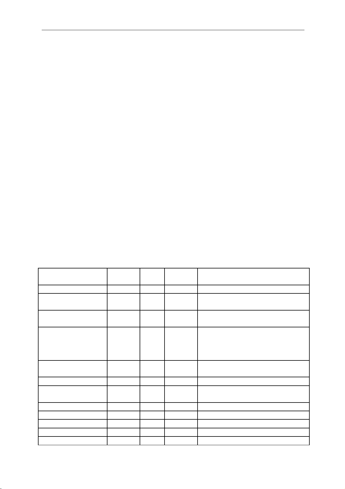
Appendices
Appendix A Servotest Extensible Format
Appendix A.1 File Identification
SEF files are identified by having the extension “.SEF”, and the first 56 bytes of the file
being a File Identifier, the Unicode string “Servotest Extensible Format.”
Appendix A.2 Arrangement of Data
Immediately following the file identifier is a list of “ID Pointer Pairs” (IPP’s). These consist
of a 32-bit identifier, a 64-bit file pointer and a 32-bit checksum of the identifier and pointer.
This list is terminated by a 32-bit integer zero.
struct ID_PTR_PAIR
{
unsigned long id;
__int64 ptr;
unsigned long checksum;
};
The ID defines what the pointer points to.
Appendix A.3 Defined ID’s
Note that ‘Required’ and ‘Default’ are mutually exclusive; if there is not a sensible default,
then the parameter must be present.
Scope is either ‘Global,’ ‘Channel,’ or ‘Either’, where a global parameter can be overridden
or replaced by one for each channel.
Descriptions of some data types appear after this table.
ID Scope Requi
red
Default Points To (Description)
ID_DESCRIPTION Global False File description (String).
ID_LOGGEDTIME Global False Date and time file was created
(SystemTime).
ID_PARENTFILE Global False File that this was derived from
(String).
ID_CHANNELS Global True Number of channels in file, as a 32-
bit integer, followed by that number
of 64-bit pointers to the channels IPP
lists.
ID_DATAFORMAT Global False Channel Specifies whether data is channel or
block multiplexed (32-bit integer).
ID_NSAMPLES Either True Number of samples (64-bit integer).
ID_SAMPLERATE Either True Number of samples per second (32-
bit float).
ID_DATA Either True The data.
ID_NPTS Global False RPC information. Only needs to be
ID_INDEP Global False Present if the file was created by a
ID_REPET Global False File Converter from a RPC file. All
ID_NFRAM Global False 16-bit integers.
1
Page 50

Appendices
ID_PTBLK Global False
ID_CH_DESC Channel False Channel name / description (String).
ID_CH_UNITS Channel False Channel Units (String).
ID_CH_SCALE Channel False Value of 1.0F in file (32-bit float).
ID_CH_RAW Channel False False Is data raw (32-bit boolean).
ID_CH_X0 Channel True * Polynomial terms for conditioning
ID_CH_X1 Channel True * Data. All 32-bit floats.
ID_CH_X2 Channel True *
ID_CH_X3 Channel True * *if data is ‘raw’
ID_CH_X4 Channel True *
ID_CH_X5 Channel True *
ID_CH_OFFSET Channel True *
ID values:
ID_DESCRIPTION = 1
ID_LOGGEDTIME = 2
ID_PARENTFILE = 3
ID_CHANNELS = 4
ID_DATAFORMAT = 5
ID_MODIFYTIME = 6 (Time file was last modified)
ID_NPTS = 10
ID_INDEP = 11
ID_REPET = 12
ID_NFRAM = 13
ID_PTBLK = 14
ID_NSAMPLES = 101
ID_SAMPLERATE = 102
ID_DATA = 103
ID_CH_DESC = 500
ID_CH_UNITS = 501
ID_CH_SCALE = 502
ID_ChannelDecimation = 503
ID_CH_RAW = 510
ID_CH_X0 = 511
ID_CH_X1 = 512
ID_CH_X2 = 513
ID_CH_X3 = 514
ID_CH_X4 = 515
ID_CH_X5 = 516
ID_CH_OFFSET = 517
Appendix A.4 String Format
When an ID points to string data, the first four bytes are an unsigned 32-bit integer, which
represents the space available for the string, i.e. the maximum length of the string. The
remaining bytes are a Unicode string.
This imposes a size limit of 4.2Gb for any string; however, restrictions imposed by the
operating system will probably be smaller.
Note that the string may not necessarily be as long as the space allocated, since it is null
terminated. For ease of editing string parameters, the space allocated should be longer than
the string
2
Page 51

Appendices
Appendix A.5 Time Format
Time is stored as a SystemTime structure.
struct SYSTEMTIME
{
WORD wYear;
WORD wMonth;
WORD wDayOfWeek;
WORD wDay;
WORD wHour;
WORD wMinute;
WORD wSecond;
WORD wMilliseconds;
Appendix A.6 Reading an SEF File
The following example is based on C but it is possible to convert these techniques to Visual
Basic, Matlab or any other programming language.
Open the file in binary mode and ensure the file pointer is at the beginning:
// file pointer to beginning
_lseek(m_hFile, 0, SEEK_SET);
// read the 56 byte file description
if (_read(m_hFile, &FileID, 56) == 56)
{
// compare the string read with what we want
if (0 == wcsncmp(L"Servotest Extensible Format", FileID, 28))
// Success, it is an SEF
return TRUE;
}
Having read the file ID start reading the header IDs and pointers. To do this we define the
following structure:
struct ID_PTR_PAIR
{
unsigned long id;
__int64 ptr;
unsigned long checksum;
};
and read it thus:
if (_read(m_hFile, &ipp, sizeof(ipp)) != sizeof(ipp))
bSuccess = FALSE;
if (!VerifyIPPChecksum(ipp))
{
if (ipp.id == LIST_TERM)
break; // This is the end of the header
else
bSuccess = FALSE; // ERROR: The checksum is incorrect and it is not the terminator
}
3
Page 52

Appendices
Where the checksum is verified thus:
#define LOLONG(i64) ((long)__int64(i64))
#define HILONG(i64) ((long)((__int64(i64) >> 32) & 0xFFFFFFFF))
BOOL VerifyIPPChecksum (const ID_PTR_PAIR& ipp)
{
unsigned long lChecksum;
// Calculate the 32 bit checksum.
lChecksum = ipp.id;
lChecksum += HILONG(ipp.ptr);
lChecksum += LOLONG(ipp.ptr);
return (ipp.checksum == lChecksum);
}
Having read the ID/pointer pair the ID is compared to the range of values described in the
table. For example if ipp.id == ID_NSAMPLES the ipp.ptr contains the offset with in the file
where the number of samples is stored as a 64-bit integer. For example:
// 64 bit value.
int64 i64Samples;
if (ipp.id == ID_NSAMPLES)
{
if (!ReadIPPParam(ipp, &i64Samples, sizeof(i64Samples)))
bSuccess = FALSE;
}
where:
BOOL ReadIPPParam (const ID_PTR_PAIR& ipp, void *Buffer, const long BuffSize)
{
__int64 OldOffset;
// Remember where we are.
OldOffset = _telli64(m_hFile);
// Go to data.
_lseeki64(m_hFile, ipp.ptr, SEEK_SET);
if (_read(m_hFile, Buffer, (unsigned int)BuffSize) != int(BuffSize))
return FALSE;
// Return file pointer.
_lseeki64(m_hFile, OldOffset, SEEK_SET);
return TRUE;
}
There must be a ID/pointer pair to indicate where the data starts, ie ipp.id == ID_DATA. By
default the data is channel multiplexed, IEEE 4-byte floats. The data is normalised to +/- 1
and is converted to engineering units using the channel scale.
4
Page 53

Appendices
Appendix B Space delimited ASCII files supported by DAP
• the file must have a .txt extension
• the first value is the Sample Rate (here 100 Hz)
• the second is the number of samples in each channel (here 21)
• the third is the number of channels (here 7)
• then come the (7) channel names (less than 20 characters)
• followed by the (7) units (less than 10 characters)
• then the data (one column per channel, space delimited)
100
21
7
Rq_Displacement FL
Rq_Displacement FR
Rq_Displacement RL
Rq_Displacement RR
speed
ax
ay
mm
mm
mm
mm
mph
g
g
0.000000e+000 0.000000e+000 4.211823e-003 0.000000e+000 0.000000e+000 0.000000e+000 0.000000e+000
8.775635e-003 4.197262e-003 1.696429e-002 -8.502663e-003 8.520971e-003 0.000000e+000 0.000000e+000
1.580803e-002 1.272295e-002 3.392857e-002 -1.700533e-002 9.089036e-002 1.363518e-004 0.000000e+000
3.335930e-002 2.465891e-002 6.645321e-002 -2.975932e-002 2.669904e-001 4.090553e-004 0.000000e+000
5.443667e-002 3.738187e-002 1.088054e-001 -5.381432e-002 6.106696e-001 8.216067e-004 0.000000e+000
7.902033e-002 6.217194e-002 1.626232e-001 -8.357364e-002 1.377557e+000 1.639717e-003 1.947813e-004
1.123994e-001 8.342058e-002 2.289594e-001 -1.076286e-001 2.402914e+000 2.734028e-003 3.895627e-004
1.492650e-001 1.037511e-001 3.081650e-001 -1.005251e-001 3.891243e+000 4.649944e-003 3.895627e-004
1.914198e-001 1.420511e-001 4.001232e-001 -2.550799e-002 6.169183e+000 7.387468e-003 3.895627e-004
2.335745e-001 2.127487e-001 4.961761e-001 1.373880e-001 8.915776e+000 1.135216e-002 5.843440e-004
2.704401e-001 3.003666e-001 5.795936e-001 3.582957e-001 1.232132e+001 1.559305e-002 3.895627e-004
3.003129e-001 3.454871e-001 6.121183e-001 5.919575e-001 1.663009e+001 2.079189e-002 8.117571e-004
3.003129e-001 2.544590e-001 5.626293e-001 8.171166e-001 2.151261e+001 2.899747e-002 2.792539e-003
2.669338e-001 -2.898734e-002 4.170875e-001 1.025324e+000 2.700580e+001 3.925532e-002 7.013810e-003
2.458564e-001 -5.002612e-001 1.540825e-001 1.207970e+000 3.313238e+001 4.240190e-002 8.410248e-003
2.880112e-001 -1.116341e+000 -2.672168e-001 1.334003e+000 3.953731e+001 3.665764e-002 6.007272e-003
4.004106e-001 -1.833548e+000 -8.580419e-001 1.345358e+000 4.613822e+001 3.104974e-002 3.604296e-003
4.952390e-001 -2.545639e+000 -1.545154e+000 1.199467e+000 5.281014e+001 2.941002e-002 1.591219e-003
4.460717e-001 -3.091939e+000 -2.175641e+000 8.921876e-001 5.924631e+001 3.939517e-002 -1.201320e-003
1.668361e-001 -3.279111e+000 -2.629464e+000 4.206127e-001 6.520531e+001 6.360285e-002 -2.402976e-003
-2.792356e-001 -3.099547e+000 -2.924877e+000 -1.416393e-001 7.100809e+001 8.740497e-002 1.591219e-003
5
 Loading...