Sencore SP395 Operation Manual

SP395 SoundPro Audio Integrator Form7492 Operation Manual

SP395

SoundPro

Audio Integrator

Operation Manual

(Firmware version 1.32)

3200 Sencore Drive, Sioux Falls, SD 57107

http://www.sencore.com

mailto:[e-mail] 1.800.736.2673 or 1.605.339.0100

SP395 SoundPro Audio Integrator Form7492 Operation Manual

WARNING

PLEASE OBSERVE THESE SAFETY PRECAUTIONS

There is always a danger present when using electronic test equipment.

Unexpected voltages can be present at unusual locations in defective

equipment and distribution systems. Become familiar with the equipment

with which you are working, and observe the following safety precautions.

Every precaution has been taken in the design of the SoundPro SP395 Audio
Integrator to insure that it is as safe as possible. However, safe operation
depends on you, the operator.

1. Never exceed the limits of the SoundPro SP395 as given in the specifications

section or other special warnings provided in this manual.

2. Always be sure that your equipment is in good working order. Broken or

frayed test leads or cables can be extremely dangerous and may expose you to
high voltages.

3. Remove test leads immediately following measurements to reduce the

possibility of shock.

4. Do not work alone when working under hazardous conditions. Always have

another person available in case of an accident.

5. Never assume that a cable shield is at earth ground potential. Both static

and electrical voltages can be present on a cable’s sheath.

6. Always follow standard safety procedures.

When in doubt, be careful.

Sencore reserves the right to make changes in specifications and other information contained in this publication
without prior notice, and the reader should in all cases consult Sencore to determine whether any such changes have
been made. This manual may not be reproduced, and is intended for the exclusive use of Sencore users.

ii

SP395 SoundPro Audio Integrator Form7492 Operation Manual

SP395

SoundPro

Audio Integrator

Operation Manual

(Firmware version 1.32)

3200 Sencore Drive, Sioux Falls, SD 57107

iii

SP395 SoundPro Audio Integrator Form7492 Operation Manual

TABLE OF CONTENTS

SAFETY PRECAUTIONS ...................................................................... inside front cover

DESCRIPTION................................................................................................................ 1

Introduction ............................................................................................................................1

SP395 Audio Integrator Features.......................................................................................... 1

Specifications......................................................................................................................... 4

Front Panel Control Descriptions ......................................................................................... 9

Right Side Panel – Input Description................................................................................... 9

Left Side Panel – Output Description ................................................................................10

SP395 Audio Integrator Accessories .................................................................................11

Firmware Add-on Test Functions ....................................................................................... 13

OPERATION................................................................................................................. 14

Power ON/OFF Switch ........................................................................................................... 14

Power Input Jack.................................................................................................................... 14

Battery.................................................................................................................................... 14

Installing/Removing Battery............................................................................................... 15

Battery Charging & Battery Life .........................................................................................15

User Interface – Control Knob................................................................................................ 16

Menu Navigation .................................................................................................................... 16

Menu Overview ......................................................................................................................17

Inputs & Outputs ....................................................................................................................18

Audio Inputs....................................................................................................................... 18

Audio Outputs....................................................................................................................19

Audio Monitoring Output.................................................................................................... 19

Input Gain Control - Preamplifiers ..................................................................................... 20

Menu Toolbars .......................................................................................................................21

Top Tool Bar......................................................................................................................21

Bottom Tool Bar................................................................................................................. 22

Headphone/Speaker Monitor Control ...........................................................................22

Memory Control ............................................................................................................23

SPL .............................................................................................................................. 24

Sound Level Meter .................................................................................................................24

LEQ ........................................................................................................................................26

Dosimeter............................................................................................................................... 27

Sound Study Graph................................................................................................................ 29

Acoustics ..................................................................................................................... 31

Real Time Analyzer................................................................................................................ 31

FFT Analyzer.......................................................................................................................... 35

Energy Time Graph................................................................................................................ 38

Reverb Decay Time................................................................................................................ 43

Multi-Band Decay................................................................................................................... 47

TDA - Time Delay Analysis......................................................................................... 50

Main Output & Generator Control ................................................................................. 23

iv

SP395 SoundPro Audio Integrator Form7492 Operation Manual

Noise Tools.................................................................................................................. 57

ALCONS ................................................................................................................................57

RaSTI .....................................................................................................................................60

STI-PA.................................................................................................................................... 63

Noise Curves.......................................................................................................................... 65

Transmission Loss ................................................................................................................. 67

Audio Stethoscope .................................................................................................................69

Tech Bench.................................................................................................................. 70

Level/Freq. Meter ...................................................................................................................71

Signal Generator ....................................................................................................................72

Amplitude Sweep ................................................................................................................... 74

Distortion Meter...................................................................................................................... 76

Phase Meter........................................................................................................................... 80

Crosstalk Meter ......................................................................................................................81

Speakers ...................................................................................................................... 82

Speaker Polarity..................................................................................................................... 82

Speaker Distortion.................................................................................................................. 84

Impedance Meter ................................................................................................................... 86

Impedance Sweep .................................................................................................................87

Cable Tester........................................................................................................................... 90

Tools............................................................................................................................. 92

USB Preamp Display & Controls............................................................................................ 92

USB Preamp Operation..................................................................................................... 93

USB Output Operation....................................................................................................... 94

Utility Function ............................................................................................................ 95

Audio Scope........................................................................................................................... 95

Save Settings .........................................................................................................................97

Setup & Calibration ................................................................................................................98

Setup – Unlock Firmware .................................................................................................. 98

Setup – General ................................................................................................................99

SPL Calibration................................................................................................................ 100

PC Interface/About............................................................................................................... 101

Computer Interface ................................................................................................... 102

Uploading Memories to the Computer.................................................................................. 102

Upgrading Firmware in SP395 ............................................................................................. 103

TerraLink Software: Real-Time Computer Interface............................................................. 104

APPENDIX A

dB SPL Scale .......................................................................................................................105

APPENDIX B

ANSI Weighting Curves........................................................................................................ 106

APPENDIX C

ANSI Balanced Noise Criterion Curves................................................................................ 107

APPENDIX D

Serial Protocol for Accessing SP395 Memories................................................................... 108

WARRANTY AND SERVICE

INFORMATION......................................................................................inside back cover

v

SP395 SoundPro Audio Integrator Form7492 Operation Manual

DESCRIPTION

Introduction

The Sencore SP395 SoundPro Audio Integrator is a quality, high-end audio and acoustic
analyzer designed for audio professionals, commercial audio installers, and audio system
engineers. Its audio analyzing functions make it attractive for virtually anyone involved with
audio acoustics or audio systems testing.

The Audio Integrator employs a powerful DSP
engine. All functions, filters, and processing
are implemented in DSP firmware algorithms.
As each function is selected, loaded into
internal memory and executed, the analyzer
takes on a completely new personality. Over
25 different test functions become possible in
one instrument.

The SP395 is especially good at multi-tasking.
It employs independent input, DSP processing,
output, monitor, and USB circuit sections. For

example, you can run the Sound Study Graph
to record SPL over time, while monitoring the
input in headphones, and simultaneously
feeding the input signals to a PC through the
USB audio interface.

The Integrator uses precision 24-bit A/D and
D/A converters, and internal 64-bit processing.
The input and output amplifier stages are fully
balanced, low noise, high-resolution gain
stages. The result is precision measurements
for accurate audio/acoustic analysis.

SP395 Audio Integrator Features

The SP395 provides multiple audio analyzing features including:

• Sound Level Meter or (SPL) Sound Pressure Level: Measures loudness of ambient

sound according to ANSI Type 1 A and C weighting networks and ANSI Class 1 octave

and 1/3 octave band filters. Selectable slow, fast, impulse, or peak sound level

measurement averaging modes.

• Leq: Measures linear averaged Sound Pressure Level over a specified period of time to

determine if noise standards are being met.

• Dosimeter: Measures noise dosage level according to ANSI S1.25-1991 and ASA 98-1991

specifications for noise studies, machinery noise evaluations, and occupational noise

analysis.

• Sound Study Graph: Analyzes and records SPL noise levels over a specified time period

from 1 minute to 24 hours, and graphs the results. Automatically runs multiple sound

studies storing up to 40 sound study tests.

• Real Time Analyzer (RTA): An audio spectrum analyzer which graphs the dB level of

each audio octave or 1/3 octave band. Fast DSP audio analyzing can be used for live music

or sound analysis. An ANSI X curve weighting network for motion picture theater setup is

included. RTA graphs can be stored to memory or compared with the “difference” mode

for before and after analysis.

• FFT Analyzer: Digital signal processing with three FFTs that graph the dB sound level

with 1/6 or 1/12 octave band resolution to 20 kHz. RTA graphs can be stored to memory or

compared with the “difference” mode for before and after analysis.

• Energy Time Graph: Graphs the arrival of sound energy to the microphone input and/or

shows the decay of sound energy in dB over time. Starts with sound initiated from the

1

SP395 SoundPro Audio Integrator Form7492 Operation Manual

SP295 generator or an external sound pickup such as a handclap. Valuable in setting time

delays from speaker to listening positions and analyzing sound decay for reflections or

decay time.

• Reverb Decay Time (RT60): Measures and computes reverb decay time or the time it

takes the sound in a room to decrease 60 dB. The measurement computes wideband RT60

(20Hz-20 kHz) or the RT60 of any octave band.

• Multi-Band Decay: Measures, computes and displays the reverb decay time RT60 for

seven audio octave bands simultaneously to identify differences in room sound absorption

characteristics in each band.

• Time Delay Analysis: Times a swept audio generator (20-20,000Hz) and tracking audio

1/12 octave band level meter, with a variable filter Q of 6 to 150, graphing the detected

level. Measurement eliminates room reverberations or echoes for accurate frequency

response testing of speakers or microphones.

• Speech Intelligibility: Measures speech intelligibility using the most popular industry

standards including ALCONS, RaSTI and STI-PA. A CD with the proper test signal for

these tests is provided.

• Noise Curve: Measures noise in a room and characterizes it to a numeric value taking into

account how the human ear hears. Performs standard NC or NCB (balanced noise curves),

RC (Room Criteria), and PNC (preferred noise curve) ANSI tests.

• Transmission Loss: Measures sound transmission loss through a partition. Computes

STC, RW and OITC standard transmission loss measurements by comparing 1/3 octave

RTAs from the source and received sound.

• Audio Stethoscope: Combines the microphone input and sensitive audio preamplifier with

the audio monitoring headphones to form an audio stethoscope. Weighted filters and

octave or 1/3 octave band filters may be selected.

• Level/Freq. Meter: Measures two channel left and right audio input levels from -120 dBu

to +40 dBu and sine wave frequency from 10 Hz to 32 kHz. Measures dBu, dBV, Vave,

Vrms, Vp-p and dBr.

• Signal Generator: Generates audio test signals including sine wave to 22 kHz, square

wave, pink noise and white noise with variable output level. Also outputs octave or 1/3

octave band limited pink noise.

• Amplitude Sweep: Plots the frequency response of audio equipment by sweeping the

generator through its frequency range and graphing the amplitude input level of each 1/12

octave.

• Distortion Meter THD: Measures THD+N (Total Harmonic Distortion plus Noise) of an

incoming signal by comparing the level of the incoming signal with the level of harmonics

and noise.

• Distortion Meter IMD: Measures IMD (Inter-modulation Distortion) of an incoming

signal by outputting a multi-frequency output test tone and measuring the distortion

components. Performs SMPTE IMD and DIN IMD tests.

• Phase Meter: Measures the phase difference between left and right input sine waves of the

same frequency.

• Crosstalk Meter: Measures the amount of dB isolation between the left and right input

audio sources or the signal bleeding from one channel into the other.

• Speaker Polarity: Determines the polarity of the speakers to determine proper wiring.

• Speaker Distortion: Tests speaker distortion, using the THD+N test function, to identify

speaker defects or performance problems.

• Impedance Meter: Measures the impedance of an audio device or component such as a

speaker. The frequency of the test is variable. Also indicates watts or amplification

required at a particular voltage.

2

SP395 SoundPro Audio Integrator Form7492 Operation Manual

• Impedance Sweep: Plots the impedance of a load by sweeping the generator through its

frequency range and graphing the impedance at each 1/12 octave step.

• Cable Tester: Provides a cable attenuation test at 1 kHz and 20 kHz, and a polarity test to

identify defective or improperly wired cables.

• USB Preamp Control: Serves as a calibrated USB microphone preamp. Use as a sound

card for a PC based analysis program or to route audio from a PC to the Audio Integrator

main outputs.

• Audio Scope: Provides a voltage vs. time graph of the audio waveform to look for

distortion or clipping.

3

SP395 SoundPro Audio Integrator Form7492 Operation Manual

Specifications

SoundCore™ Module

Sound Level Meter (SLM): Measures ambient sound energy levels at microphone input

Displays true RMS SPL
Averaging: Meets ANSI S1.4
Slow
Fast
Impulse
Peak
Avg – Equal time-averaged SPL

Sound Study Graph (SSG): 1 minute to 24 hour continuous recorded SPL measurement

“Strip Chart Recorder”

Peak or Avg mode

Auto-Saves to internal memory

SPL/SSG Measurements

Weighting networks: ANSI Type 1 A, C, Flat, octave, or 1/3-octave band filtered
Level Range: 25-140 dBA with MIC-TP2 mic
Level Accuracy: ±0.1 dB at 1 kHz with MIC-TP2 mic
Level Resolution: 0.1 dB
Frequency Range: 20 Hz to 22 kHz

Real-Time Analyzer (RTA): Plots sound energy levels vs. octave band filtered spectrum
ANSI-compliant 1/3 octave digital filter-based

FIR Filters: Full octave, 1/3 octave frequency resolution.
Weighting networks: Flat, A, C, X-curve, difference mode.

FFT Analyzer (FFT): Plots sound energy levels vs. octave band filtered spectrum

ANSI-compliant 1/12 octave resolution

Three 1024-point cascaded FFTs

Weighting networks: Flat, A, C, difference mode.

RTA, FFT Analyzer

Display range: 30 dB or 15 dB window within 0 dB to 165 dB range, adjustable in

5 dB steps
Level range: 25-140 dBA with MIC-TP2 mic
Level accuracy: ±0.1 dB at 1 kHz with MIC-TP2 mic
Level resolution: ±0.1 dB
Frequency range: 20 Hz – 22 kHz
Frequency accuracy: ±0.5 dB 10 Hz to 22 kHz, ±0.2 dB 100 Hz to 16 kHz
Averaging: 1 sec, 3, sec, 6 sec, 10 sec, 30 sec, 60 sec, equal time-weighted,
peak hold

4

SP395 SoundPro Audio Integrator Form7492 Operation Manual

Energy-Time Graph (ETG): Graphs impulse sound decay energy vs. time or distance

Identifies arrival time of direct sound and audio reflections
Displayed in mS (milliseconds), ft (feet), m (meters)

Decay time ranges: From 0-15 mS to 0-7680 mS

Calculates RT10-RT60 from cursor points on decay curve

Accuracy: Better than ±1% of full scale

Reverb Decay Time: Calculates time for residual pink noise test signal to decay 60 dB in

room

Also RT10, RT20
Range: 0-15 sec
Accuracy: ±2% of full signal
Resolution: 1 mSec
Weighting networks: A, C, Flat, octave, or 1/3-octave band filtered.
Ambient Noise: Ambient noise level must be at least 26 dB lower than test signal
RT60 Time: Extrapolated from Decay Time measurement.

Impedance Meter:

Accuracy: 1 ohm to 50 ohms, ±2%, 50 Hz – 12.5 kHz

1 ohm to 8 kohms, ±10%, 20 Hz – 20 kHz

Speaker Polarity: Tests absolute speaker phase (polarity) by analyzing a proprietary
waveform

Shows polarity of mid-frequency wavefront
Range: 0-100 ft, speaker to SoundPro

Cable Tester: Tests XLR, 1/4”, and RCA audio cables, balanced and unbalanced

Performs analog transmission test to test transmission loss at 1 kHz and 20 kHz

Resolution: 0.1 dB

Performs polarity test

Signal Generator:

Signals: Sine, square, gaussian white noise, pseudo-random pink noise,
band-filtered pink noise
Frequency Range:

Sine: 1 Hz to 22 kHz; fine, 1/3 octave, or one octave steps
Square: 1 Hz to 6 kHz; fine, 1/3 octave, or one octave steps

Noise bandwidth: Full (20 Hz to 20 kHz), octave, or 1/3-octave band filtered
Frequency Accuracy: 50 ppm; 0.005%
Level range: -35 dBu to 17 dBu
Maximum Sine Output Level: Balanced: +16 dBu

Unbalanced: +10 dBu

Level Accuracy: ±0.1 dBu at 1 kHz, ±0.2 dBu, 16 Hz to 20 kHz

Typical: ±0.05 dBu at 1 kHz, ±0.1 dBu, 16 Hz to 20 kHz

Sine distortion: < 0.01% THD at full-scale output

Audio Monitor: Source independent channel for monitoring

Software volume control
Headphone or built-in internal speaker output

5

SP395 SoundPro Audio Integrator Form7492 Operation Manual

TechBench™ Module

Level Meter: Stereo level meter reads in dBu, dBv, Vp-p, Vrms, or dBr
(reference)

Frequency Range: 10 Hz to 22 kHz
Auto-level ranging.

Level Range: -120 dBu to +40 dBu

Level Accuracy (–85 dBu to +40 dBu): ±0.2 dB, 10 Hz to 22 kHz

Typical: ±0.01 dB, 100 Hz to 16 kHz; ±0.05 dB, 10 Hz to 22 kHz

Level Resolution: 0.01 dBu

Frequency Counter:

Frequency Range: 16 Hz to 40 kHz
Accuracy: ±5%
Resolution: 1 Hz

Amplitude Sweep: Graphical display of 1/3 and 1/12 frequency response

User adjustable frequency range

Impedance Sweep: Graphical display of 1/3 and 1/12 octave impedance values

User adjustable frequency range

Distortion Meter: THD+N – Computes Total Harmonic Distortion plus Noise

Compares level of output harmonics and noise to single test frequency

Test Frequencies: 63 Hz, 125 Hz, 250 Hz, 500 Hz, 1 kHz, 2 kHz, 4 kHz

IMD – Computes Inter-modulation Distortion
Compares levels of output sum and difference frequencies to dual test frequencies

Test Types: SMPTE 60/7kHz, DIN 250/8kHz.
Inputs: Speaker, microphone, line level.
Range: 0.02% to 50% THD+N
Accuracy: ±5% of reading

Phase Meter: Shows the phase difference in degrees between 2 sine waves

Crosstalk Meter: Displays the amount of isolation that exists between two audio

sources

Displayed in dB

Audio Scope: Shows audio signal on an oscilloscope-like screen

Dual-trace, auto-triggering
AC-only input coupling (down to approx. 3 Hz)

X-Y mode for phase display
Sample rate: Hz
Accuracy: ±1 display pixel

6

SP395 SoundPro Audio Integrator Form7492 Operation Manual

Speech Intelligibility Module: (RaSTI and STI-PA test waveforms included on CD)

ALCONS: Computes Percent Apparent Loss of Consonants
RaSTI: Calculates Rapid Speech Transmission Index
STI-PA: Computes Speech Transmission Index using STI-PA method

(STI for Public Address)

Time-Delay Analysis Module:

Time-Delay Analysis: Measures frequency response using log-swept sine wave.

(TerraLink software included)

Noise Curves Module

NC Curves: Displays Noise Criteria data, based on ANSI standard S12.2-1995

(ASA 115-1995)

Displays limiting band, SPL by octave band

RC Curves: Displays Room Criteria rating
PNC Curves: Displays Preferred Noise Criteria rating
STC/NIC Measurement: 1/24th octave Sound Transmission Class/Noise Isolation Class

measurement

Multi-Band Decay Module

Multi-Band Decay: Displays seven octave-band filtered RT60 measurements

simultaneously

Audio Stethoscope Module

Audio Stethoscope: Filters incoming left input audio through to the headphone or
speaker

Filters: Flat (no filter), A or C ANSI Weighted, octave, 1/3 octave filters

Audio Hardware

Sample Rate: 48 kHz
Input Gain Ranges: -50 dB to +50 dB
Maximum Rated Input: +40 dBu

Preamplifier

Distortion: -90 dB THD+N
Phantom Power output: 48 VDC ± 1 VDC

ADC/DAC

Cirrus Logic: CS4224 48 kHz 24-bit 105 dB Audio CODEC

USB Preamplifier

Burr-Brown Texas Instruments® USB Audio CODEC
USB 1.1 full-speed
USB isochronous data format

7

SP395 SoundPro Audio Integrator Form7492 Operation Manual

Standards

Sound Level Meter: ANSI S1.4-1983 (ASA 47-1983)
Leq: ANSI S1.43-1997
Dosimeter: ANSI S1.25-99 (ASA 98-1991) Class 2
Digital Filters: ANSI S1.11-1986 1/1, 1/3 octave digital filters

All filters, weighting networks, response rates, and algorithms meet or exceed ANSI

Type 1 specifications

General/Environmental

Input Impedances

XLR and balanced inputs: 40 kohms nominal
RCA unbalanced inputs: 20 kohms nominal

Output Impedances

XLR and balanced outputs: 300 ohms nominal
RCA unbalanced outputs: 150 ohms nominal
Non-Volatile Memory: 40 graph data storage locations
Display: 64x128 pixel blue LCD with backlight
Size: 9 1/2" x 5 1/2" x 2 1/4" (HWD)
Weight: 2 lbs. 5 oz.

Temperature Range: 5°C to 45°C, non-condensing
Power

Battery: Li-Ion pack provides over 5 hours of service, depending on usage
AC adapter/charger: 120/130/230/240 VAC, 9-12VDC, 800 mA (Nominal 9V)

8

SP395 SoundPro Audio Integrator Form7492 Operation Manual

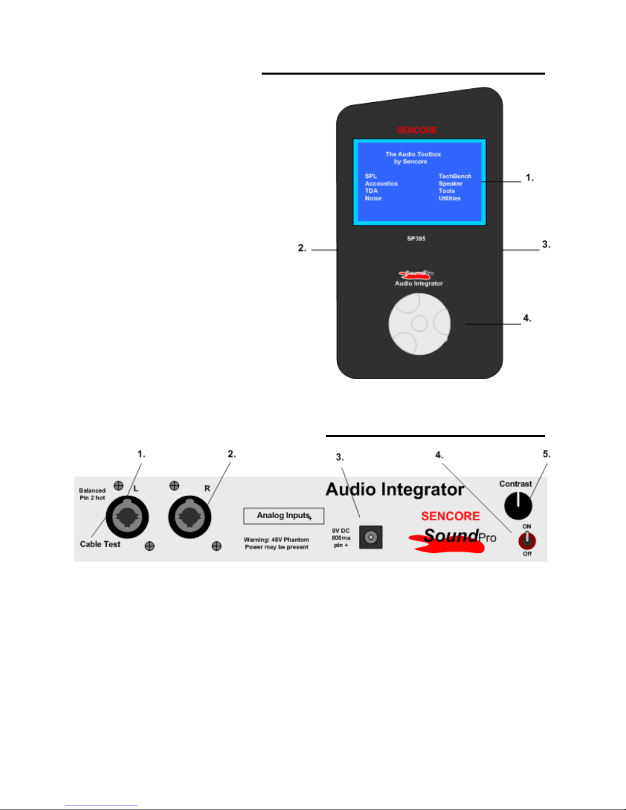
Front Panel Description

1. Display Screen: Provides a visual

interface to the user of all instrument
functions and test results.

2. Left Side Panel: Contains

Computer, USB and analog audio
jacks and speaker. See Left Side
Panel Description section for details.

3. Right Side Panel: Contains power

input jack, audio input jacks, on/off
switch and contrast control. See
Right Side Panel Description section
for details.

4. Control Knob: Provides navigation

through instrument menus. All test
operations and user selections are
performed using this control. This
control is both rotated and pressed.
Rotate the control to move the
screen cursor or increment through menu selections. Momentarily pressing inward
(clicking the control knob) makes a selection or change.

Right Side Panel – Input Description

1. Left Analog Input: Combination XLR and ¼ inch Balanced Microphone /Line input.

Used as main input for most tests. May have 48 Volt Phantom Power switched to jack by
instrument. Used as Cable Test Input.

2. Right Analog Input: Combination XLR and ¼ inch Balanced Microphone /Line input.

May have 48 Volt Phantom Power switched to jack by instrument.

3. Power Adapter Input: Powers the instrument and charges the internal rechargeable

battery. Use a Sencore approved adapter nominal 9V @ min 800 mA. (Center pin
positive)

4. Power Switch: Turns the instrument power on or off. Down is Off.

5. Contrast Control: Sets the contrast of the display screen for best viewing.

9

SP395 SoundPro Audio Integrator Form7492 Operation Manual

Left Side Panel – Output Description

1. RS232 Computer Interface Connector: Serial DE-9 connector. Interfaces instrument to

computer for use with automation software and for the purpose of updating unit firmware
to factory changes.

2. USB Audio Connector: Provides USB connection for digital audio signals.

3. Stereo Headphone (Hdpn) Output Jack: ¼ inch headphone jack. Provides stereo audio

monitoring with headphone.

4. RCA Phono Audio Output Jack: Provides unbalanced audio output through female

RCA phono jack.

5. Balanced mono Audio Output Jack: Provides balanced audio output through a ¼ inch

headphone jack (TRS).

6. Balanced XLR Audio output: XLR jack male, Provides a balanced mono audio output.

Jack also used for Cable Test output.

7. Internal Speaker: Provides audio output to monitor input audio to instrument or audio

generated and output by instrument.

10

SP395 SoundPro Audio Integrator Form7492 Operation Manual

SP395 Audio Integrator Accessories

Sencore
Part #s

133G527

13G122

13G123

Description Photo

TerraLink Viewer Software /Speech
Intelligibility Audio CD provides

TerraLink – viewer only capability – along
with the audio CD files needed for the
STIPA and RASTI speech intelligibility
tests.

supplied

XLR Audio Cable – a microphone cable

for interfacing balanced audio inputs and
outputs to the SP395.

supplied

USB Cable – a 6’ connection cable (type

A to type B), connects the unit’s USB
connector to a USB port on a computer
PC USB port.

supplied

Serial Interface Adapter Cable – a 6’

computer serial interface adapter cable

13G124

17G65

39G1156

(straight through), connects between the
unit’s RS232 jack and a computer serial
port.

supplied

Lithium Ion Battery – install battery to

power the instrument. The battery is
removable, supplies up to 5 hours of
continuous power per charge, depending
on use.

supplied

Standard Measurement Microphone

meets or exceeds ANSI Type 2
specifications. Microphone Holder Clip
mounts on a standard microphone stand
and holds the test microphone.

Both are supplied.

11

SP395 SoundPro Audio Integrator Form7492 Operation Manual

Impedance Test Cable 1/4 inch mono
plug to clip connections – provides a test

39G1171

60G80

lead connection when using the
Impedance Meter and Impedance Sweep
test functions.

supplied

AC Power Adapter/ Charger plugs into

the SP395 to charge the battery or to
provide AC operation.

supplied

Soft Carry Case padded carrying case to

CC309

SP­PMIC1

optional

SPSW-TL

optional

transport unit; includes extra storage
capacity for supplied accessories.

supplied

Precision Low Noise Microphone –

meets or exceeds ANSI Type 1
specifications

optional

Software – provides a real-time PC

connection/interface with the instrument.
Plots memories and displays FFT, RTA,
SSG and SLM Meter results in real-time.
(Requires purchase and authorization of
an UNLOCK code from Sencore) Included

as part of the Time Delay Analysis (TDA)
Firmware Add-on Module. optional

Terra Link Software Unlock
Code

http://www.sencore.com mailto:[e-mail] 1.800.736.2673

12

SP395 SoundPro Audio Integrator Form7492 Operation Manual

Firmware Add-on Test Functions

The Audio Integrator comes standard with a solid core of audio analyzing tests. These tests are
fundamental to most audio and acoustic analysis work. The core tests are referred to as the
SP395’s “SoundCore” measurements.

The Audio Integrator contains, in its internal operating software or firmware, instructions for
performing many more audio and acoustic tests than provided by the standard “SoundCore”
measurements. These additional tests may be purchased based upon individual user and company
requirements. The additional available tests are divided into packages or “Firmware Modules”
for easy implementation or purchase.

Firmware Module Function Menu

TechBench Amplitude Sweep TechBench

TechBench Distortion Meter TechBench

TechBench Phase Meter TechBench

TechBench Crosstalk TechBench

TechBench Audio Scope Utilities

TechBench Impedance Sweep Speaker

Noise Curves NCB, RC, PNC Noise Tools

Noise Curves Transmission Loss

(RW, STC, OITC)

Speech Intelligibility ALCONS, RASTI,STI-PA Noise Tools

Time Delay Analysis TDA TDA

Audio Stethoscope Audio Stethoscope Noise Tools

Multi-Band Decay RT60 Multi-Band Decay Acoustics

The optional functions are available for use upon purchasing the firmware module and entering
the supplied unlock code. The functions contained within a single firmware module may appear
on more than one menu. The table lists the firmware modules and the functions they contain,
along with the Audio Integrator menu that the function appears in.

To purchase an unlock code for a firmware module, contact Sencore. For instructions on how to
unlock a firmware module, see the Setup & Calibration section of this manual.

Specifications, accessories and software add-on test functions are subject to change without
notice.

Noise Tools

13

SP395 SoundPro Audio Integrator Form7492 Operation Manual

OPERATION

Power On/Off Switch

The power switch is mounted at the top of the right side panel. The power switch turns the Audio
Integrator on or off, whether the unit is powered by the internal battery or the AC adapter.
When you turn on the power switch, the unit begins initialization. During this time software is
loaded from memory locations within the Audio Integrator including updates. The unit is ready
to use as soon as the main menu screen appears, no warm-up time is needed. The Audio
Integrator can be powered off at any time – there is no required shutdown procedure.

Power Input Jack

The Power Input Jack is located in the center of the right side panel. The DC Input Jack requires
the input of a DC voltage to power the instrument and charge the internal battery. The SP395
requires a 9-12v DC power adapter, regulated or unregulated, rated at a minimum of 800ma. The
input connector is a 2.1mm coaxial power connector with the positive polarity voltage on the
center pin of the connector.

An AC power adapter/charger is supplied to power the Audio Integrator and charge the internal
battery. Use only the Sencore-supplied power adapter, if possible. Using an improper AC adapter
can damage the unit and/or improperly charge the battery. Using an improper AC power
adapter/charger voids the unit warranty.

The AC plug symbol in the display screen beside the < (back) field indicates the
unit is powered form the AC power adapter/charger.

When the AC power adapter is plugged in, the battery level indicator
shows an AC power plug symbol. When the AC power adapter is
removed, the indicator shows a battery symbol with a relative battery
charge level.

Battery

A lithium-ion rechargeable battery is supplied with the Audio Integrator. The battery is charged

whenever the AC adapter is plugged in, or can be charged using an
external charger.

Battery operation is indicated with a battery symbol near the < (back) field. The
symbol indicates the approximate charge level of the battery.

Battery operation is indicated in the Audio Integrator screens with a
battery symbol located in the upper left of the screen adjacent to the <
(back field). The symbol also indicates the relative charge of the
battery. It the battery symbol is filled to the top, the battery is at or near
full charge. A battery symbol that shows little or no fill indicates that

the battery is nearing a discharge level in which it must be recharged.

14

SP395 SoundPro Audio Integrator Form7492 Operation Manual

Installing / Removing Battery

The battery can be removed for replacement. The battery is installed in a small compartment in
the bottom rear of the Audio Integrator. To remove the battery you must open the battery door or

cover plate. Unscrew the thumb screw holding
the plate to the instrument case. The door
contains a cutout so if you push the door away
from the screw the door can be hinged open. Use
the nylon strap that surrounds the battery to lift
it up and out of the compartment. The battery
terminals plug into the small circuit board lining
the top side of the battery. Gently pull the circuit
board away from the battery to disconnect the
battery from the circuit board.
To install a battery, reverse the removal process.
The battery is polarized and needs to be installed
correctly. Line up the flat side of the battery
with the flat side of the circuit board. Push the
board male connector pins gently and straight
into the battery terminals. Seat the battery into
the instrument, close the battery door and secure
it by tightening the retainer screw.

The battery may be removed from the rear battery compartment.

Warning: Observe proper polarity. Do not plug the battery into the connector board the
wrong way, or the battery may be damaged.

Battery Charging & Battery Life

The battery is charged anytime that the AC adapter is
plugged into the Integrator. It charges at the same

Charger Charge Time

Charge in Integrator 6.0 hours
rate, whether the unit is turned on or not. You can
also charge the battery in an external lithium-ion battery charger. You cannot overcharge the
battery, as long as you charge it in the instrument or use an approved external charger. The
battery requires about 6 hours to fully charge.

The Audio Integrator uses different amounts of
battery power, depending on what functions are
being used. The phantom power uses a significant
amount of power. Also, the headphone monitor

Battery Life

Maximum run time 5.5 hours

Phantom power on 4.5 hours

amplifier consumes power when it is enabled. Expect 4-5 hours of run time on a full charge.

Warning: Storing the unit with the battery in a state of discharge for long periods of time can
shorten the life of the battery, or possibly destroy it. We recommend that the battery be kept
charged at all times. The battery cannot be overcharged, so it is fine to leave the instrument
plugged in, or to leave the battery plugged into an external charger when not in use.

15

SP395 SoundPro Audio Integrator Form7492 Operation Manual

User Interface – Control Knob

All the Audio Integrator operations and user selections are performed using the front panel
control knob. This control is either rotated or momentarily pressed (clicking) the control knob.
Turning the control knob moves a display highlight (white box with dark text) between menu
options and fields on the screen. Clicking a highlighted choice selects it. To exit from a function
and return to the previous menu or screen, highlight and click on the “<” symbol located in the
upper left corner of the display.

To change the value of a selected field, click the control knob. The highlighted field will either
toggle to a new value (fields with only a few possible values) or will change to an underlined
“control lock” (data with many possible values).

To change the value of a “control-lock” field, click the control knob to “lock” (underline) the
field and then turn the knob to change the value. When the desired value is shown, click the
control knob again to unlock the control highlight. Turning the knob then moves you to the next
field

All user selections are made using the control knob either by rotating it to select a menu field or
by momentarily pressing or “clicking” the knob to increment values or lock to a field.

Menu Navigation

The main menu with eight main function categories appears shortly after the Audio Integrator is
turned on. By default the first item or category is highlighted. Turn the control knob to highlight
the different menu items and click the control knob to select the item or category. A sub-menu
appears with fields that list test functions that can be selected for that category. To select a
function in the sub-menu, turn the control knob to highlight the desired field or function and
click the control knob (press down momentarily). To exit from a sub-menu back to the main
menu move the highlight to the upper left “<” field and click the control knob.

Click the < field located in the upper left corner of every display to
return to the previous menu.

16

SP395 SoundPro Audio Integrator Form7492 Operation Manual

Menu Overview

All user selections to configure the Audio Integrator are performed with indications in the
display screen. The Audio Integrator includes a main menu with eight categories of tests in
which to choose from. Choosing a category in the main screen results in a submenu. The
submenu lists all the tests available in that category.

Note: Some of the tests shown in the submenu screens may not be included in your Audio
Integrator. These test features may be purchased as Software Additions to your
instrument.

1. Main Menu: Opening menu screen listing eight categories of Audio Integrator tests.

2. SPL Submenu: Appears when the SPL selection is made in the main menu. This

submenu lists the sound level measurements available for selection using the Audio
Integrator.

3. Acoustics Submenu: Appears when the Acoustics selection is made in the main menu.

This submenu lists the acoustic analyzing tests available for selection using the Audio
Integrator. Note: The Multi-Band Decay tests is available as a firmware option. It
appears in submenu but cannot be implemented without purchasing an unlock code.

17

SP395 SoundPro Audio Integrator Form7492 Operation Manual

4. TDA Submenu: Appears when the TDA selection is made in the main menu. This

submenu shows the TDA test functions available on the Audio Integrator.

Note: The TDA tests are optional firmware add-on test functions.

5. Noise Tools Submenu: Appears when the Noise selection is made in the main menu.

Provides noise related measurements using the Audio Integrator. Note: The ALCONS,

RaSTI, and STI-PA are speak intelligibility tests available as part of the Speech
Intelligibility firmware option. The Audio Stethoscope is available as a Stethoscope
firmware option.

6. TechBench Submenu: Appears when the TechBench selection is made in the main

menu. Provides selection of audio bench testing functions. Note: The Amplitude Sweep,

Impedance Sweep, Distortion Meter,, Phase Meter, and Crosstalk Meter are part of the
TechBench firmware option.

7. Speakers Submenu: Appears when the Speaker selection is made in the main menu. The

submenu provides selection of speaker related tests.

8. Tools Submenu: Appears when the Tools selection is made in the main menu. This

submenu provides a selection for USB Preamp Control.

9. Utilities Submenu: Appears when the Utilities selection is made in the main menu. The

Utilities Functions submenu provides user options to save settings, calibrate and interface
the Audio Integrator. Note: The Audio Scope function is part of the TechBench firmware
add-on option.

All test functions available for the Audio Integrator are listed in the submenus. This includes all
functions which are part of the standard or “Sound core” tests and test functions which can be
added with firmware add-on purchases. If you select a test in the submenu that has not been
added with a firmware purchase, the instruments indicates an “unlock required” message.

Inputs & Outputs

Audio Inputs

The Audio Integrator receives audio signal inputs from a microphone or line input
The input signal jacks are located on the right side of the instrument. There are two input jacks
which are labeled left (L) and right (R). The input jacks are a combination connector which
accepts a balanced XLR connector male input and a ¼ inch stereo mono headphone male
connector. This provides compatibility with most audio microphone cables and line input cables.

Left side input signal connectors are a combination XLR and ¼ inch mono headphone jack

18

SP395 SoundPro Audio Integrator Form7492 Operation Manual

The left (L) input should be considered as the main channel input when using the Audio
Integrator. Some test functions, such as the cable test and audio stethoscope, only use one input.
In these cases you always use the left (L) input connector when performing the test.
Be aware that the different test functions of the Audio Integrator are setup for a mic. Level input
and others for a line level input. In each case, the input signal is taken from the left and right
input jacks. For the acoustics test functions, a microphone is normally connected, and for the
TechBench tests, a line level (or lower) electrical audio signal is anticipated by the SP395.

The acoustics functions, which expect input from a microphone, use the microphone SPL
calibration that is stored in the Utilities Calibration section. Electrical functions, which expect
their input from a line level source, use the dBu calibration. Keep this in mind to prevent
potential confusion over measurement results. For example, if a 0 dBu electrical signal is
plugged into the Sound Level Meter, you may see results like +150 dB SPL, depending on the
sensitivity calibration that is stored. Conversely, if you are using a microphone with the
Amplitude Sweep function, you will see very low results, perhaps in the –70 to –60 dBu range.

Audio Outputs

The Audio Integrator provides 3 output jacks for connecting analog audio output to sound
systems. You may use either the XLR, 1/4” TRS, or RCA phono jack. These jacks are located on
the left hand side of the instrument. All carry the same signal. The output range of the Audio
Integrator is approximately -72 dBu to +17 dBu.

The left side panel contains three analog audio outputs including an XLR, ¼ TRS headphone mono, and
unbalanced RCA phono jack.

Use the XLR male output jack when a balanced XLR audio output is needed. The ¼ inch TRS
headphone jack output is available when this connection is desired. This connector is wired in
parallel with the XLR output jack. It provides a TRS (tip, ring, sleeve) balanced audio output.
One side of the balanced output is routed to the RCA phono to form an unbalanced output. Use
this jack when you desire connection to an RCA connection cable.

Audio Monitoring Output

The Audio Integrator provides a headphone output jack for monitoring output audio. It is a stereo
output headphone jack with the purpose of simultaneously monitoring both a right and left audio
channel. The stereo headphone jack powers 32 ohm or grater headphones. The headphone jack
can also serve as a line level output if needed.

A speaker is built into the Audio Integrator for the purpose of monitoring the output audio. The
speaker is located on the left side panel of the instrument. The internal speaker outputs the mixed
left and right outputs taken from the headphone output.

19

SP395 SoundPro Audio Integrator Form7492 Operation Manual

The audio output from the headphone jack and speaker is routed through separate output
monitoring circuits within the Integrator. Audio to the headphone or speaker is independently
switched on or off in the monitor part of the menu screen. The audio level output to the
headphone and speaker is controlled in the monitor part of the menu screen. Internal generated
audio or audio to the input jacks of the Audio Integrator may be routed to the monitor circuits.
Right, left, stereo, mixed (mono) audio may be selected. See the Bottom Toolbar section of this
manual.

Input Gain Control - Preamplifiers

The left and right audio inputs of the Audio Integrator feed into separate audio preamplifiers and
gain control circuits. These circuits provide audio measurement over a wide range of audio levels
and provide great sensitivity. There are thirteen gain ranges that are available to set the level of
both the left and right input audio signal. The gain ranges of the left and right inputs are
controlled independently in the top toolbar section of the test menu. See the Top Tool Bar
Section of this manual.

The selected input level or gain control setting establishes an overall amplification of the input
signal and best signal-to-noise ratio. The gain setting must be properly chosen for proper testing
results. You should select the range which provides the most amplification without overdriving
the sensitive input pre-amplifiers. The table below defines the clip points of each gain setting,
both in dBu and related for available standard microphones.

Clip Points Table

Gain Setting

Line Input

( dBu)

MIC-TP2
( dB SPL)

MIC-TP1
( dB SPL)

58 -45
52 -39
46 -34
40 -29 110 80
34 -23
28 -16
20 -9 130 100
10 1 140 110

-10 15 160* 130

-20 25 170* 140

-30 35 180* 150*

-40 45 190* 160*

* Beyond microphone maximum level

Note: To get the lowest SPL or noise levels you should use the maximum input gain setting
possible without clipping. In many cases this will be 42-58. At this setting you will have the most
sensitivity, but the input may clip at normal room SPL levels, depending on the sensitivity of the
microphone.

The Audio Integrator provides both manual and automatic range selection for the left and right
audio channels. The auto-gain function selects an input range for best measurement. If the input
level gets within 2dB of clipping, the gain is set to the next least sensitive gain (if possible). If
the input level is below that level at which the most accurate measurements can be made, the
gain is increased in steps until the maximum input gain is reached.

20

SP395 SoundPro Audio Integrator Form7492 Operation Manual

The Audio Integrator provides an indication when the input level is approaching or overdriving
the input preamplifier. The range number in the top tool bar of the menu blinks. When you see
this select a higher gain setting in the top toolbar for that channel.

Menu Toolbars

The Audio Integrator uses “toolbars” to provide access to often-used features and controls.
Toolbars along the top edge and bottom edge of the screen provide user selections which are
common to many of the test functions. For example, you can adjust input gain, turn phantom
power on and off, and control the generator output and the headphone monitor from any screen
using the top SP395. It is important that you understand the use of the toolbars to properly
operate the SP395. Individual items which can be selected and changed are referred to as fields
in this manual.

Toolbars along the top edge and bottom edge
of the screen provide user selections which are

common to many of the test functions

.

Top Tool Bar

The top toolbar provides a function identification field and is used to control the SP395 inputs.
You can manually select input gain, turn on phantom power, or invert the phase of either channel
independently. You can also enable auto-gain scaling for both inputs.

The Top Tool Bar provides function
identification and selections for the L & R
inputs.

Top Toolbar Icons

1. Back Arrow. Clicking on this icon exits the currently running function and returns to the

function menu.

2. Battery Indicator. When operated on the internal battery, this field shows the relative

battery level, or remaining charge, in the battery. When operated in AC mode, this field
shows the AC power symbol.

3. Screen Title. This is the abbreviated name of the function that is currently running.

4. Function related selection – Not on all menus

5. Left Input Polarity The N/R icon changes the left input from normal (N) polarity to

reverse (R) polarity.

6. Left Input Phantom Power Click to select the icon, then turn clockwise to enable

phantom power (48v), or counter-clockwise to disable phantom power (0v).

21

SP395 SoundPro Audio Integrator Form7492 Operation Manual

7. Left Input Gain There are 12 selectable input gain settings. Click and turn to select the

gain for this channel. A blinking value or digits indicate clipping and the need to reduce
the gain selection number.

8. Auto-Gain. Select manual (M) or auto (A). In auto-gain, the gain setting for the channel

is automatically adjusted to prevent clipping and to have enough gain for accurate
measurements. Note that in some functions, such as Leq, you may want to hold the gain at
a fixed level. In this case, choose manual (M).

9. Right Input Gain There are 12 selectable input gain settings. Click and turn to select the

gain for this channel. A blinking value or digits indicate clipping and the need to reduce
the gain selection number.

10. Right Phantom power Click to select the icon, then turn clockwise to enable phantom

power (48v), or counter-clockwise to disable phantom power (0v).

11. Right channel polarity reverse The N/R icon changes the left input from normal (N)

polarity to reverse (R) polarity.

Bottom Tool Bar

The bottom toolbar contains three functional control sections. The sections include:

1. Headphone/Speaker Monitor

2. Memory

3. Output Generator

All or part of the bottom tool bar sections or
selections within each section may be
present in the various test functions of the
Audio Integrator.

The Bottom Tool Bar provides
headphone/speaker, memory, and internal
generator control.

Headphone/Speaker Monitor Control

The five icons at the left end of the bottom toolbar control the monitor output.

1. Monitor Output On/Off The 1/0 icon turns the analog monitor output on and off. This

controls both the headphone jack and the built-in speaker.

2. Level The bar level gauge icon controls the analog output level. Every turning step of the

control knob changes the output level by approximately 1 dB.

3. Speaker On/Off. This icon turns the speaker on and off. The speaker can be turned off,

even when the headphone output is enabled. To hear the speaker output, both the Monitor
On/Off and the Speaker On/Off must be turned on.

4. Source The I/O source icon determines the source for the monitor output. The I selects

the Input for monitoring, the O selects the Output signal (usually the internal digital
generator) for monitoring. Therefore, in Input mode you will hear exactly what is being
received, as selected by the input select field on the top toolbar, and in Output mode, an
exact copy of the digital output signal will be routed to the headphone jack.

5. Mode. The monitor mode field changes between stereo (S), left mono (L), right mono

(R), and the mixed left and right channels (M).

Headphone Warning: Be careful when wearing headphones and changing input connections,
input gain, and phantom power. Although the analog output is usually muted in situations that may
cause high output, unexpected loud volume may occasionally occur at the headphone output. We
recommend turning off the output before changing functions, and in other situations that may cause
loud volume.

22

SP395 SoundPro Audio Integrator Form7492 Operation Manual

Memory Control

Some test functions support saving measurement data to internal, non-volatile memory. The
SP395 provides memory storage of RTA, FFT, ETG, Dosimeter, Sound Study Graphs,
Amplitude Sweep and Impedance Sweep functions. These functions use the four memory control
icons, in the center of the bottom toolbar. Note that a memory must be empty (cleared) before
measurement data can be stored into it. The Clear (C) icon can be used to erase the contents of a
memory.

6. Memory Number The memory number icon selects a memory location for storing,

recalling, or clearing. There are memory numbers 0 through 39 or 40 locations. When the
memory number field is selected, the type of data stored in that location (or “---” if
empty) appears on the bottom of the graph.

7. Store Click the S (Store) icon to store the results of the current function. The memory

location must be available (empty) before storing results. If the function does not support
memories, the icon does nothing.

8. Recall Click the R (Recall) icon to retrieve the results stored in the current memory

location and to display them on the screen. If the current function does not support
memories, the icon does nothing.

9. Clear Click the C (Clear) icons to erase the contents of the current memory location.

Main Output and Generator Control

The five icons that control the main output and signal generator are located on right end of the
bottom toolbar. Some fields control only the generator, while others control features of the main
output section.

10. On/Off The 1/0 icon turns the generator on and off. This field also controls functions that

use special output signals, such as the transparency test.

11. Level The bar level gauge controls the digital generator output level. Every turning step

of the control knob changes the output level by exactly 1 dB.

12. Waveform This icon selects the generator waveform. It can also select the USB input as

a signal source. The available waveforms are sine, square, white noise, and pink noise.
The USB selection sets up the USB input as a source for the main output.

13. Select Frequency This field changes the frequency of the generator output, as

determined by the Step Size field.

14. Step Size This field selects how the frequency field changes the generator frequency.

Choices are octave steps (Oct), one-third octave steps (1/3), or fine mode (Full). In full
mode the generator frequency is selectable in 1 Hz steps to 10 kHz and 2 Hz steps above

10 kHz.
In some functions the output generator is required to be in set conditions to perform the test
function. Examples include the Impedance Meter, the Cable Tester, and the Sweep tests. In these
functions, some icons on the bottom toolbar will not appear. However, even if generator settings,
levels, and other items are changed, the settings that were in effect most recently will re-appear
when a function is selected that uses the normal toolbars.

23

SP395 SoundPro Audio Integrator Form7492 Operation Manual

SPL

The SPL main menu selection provides several functions that are used in measuring Sound
Pressure Level (SPL). SPL typically uses a microphone as an input. The standard input for the
SPL tests in the left (L) input.

The SPL tests that are available on the SP395 include:

Sound Level Meter: Measures sound pressure level in dB.
Leq: Measures linear averaged sound pressure level over

time.
Dosimeter: Measures sound dosage according to ANSI or
ASA specifications.
Sound Study Graph: Graphs sound level changes over
time.

Sound Level Meter

A sound pressure level meter measures the
changes in air pressure created by sound
waves and displays this pressure as a dB level,
relative to the threshold of hearing sound
pressure. Weighting curves are added to SPL
measurements to make SPL readings
correspond to perceived loudness. The
SP395’s Sound Pressure Level function
measures the loudness of the ambient sound
level in standard dB SPL measurement units,
auto ranged from 30 to 130 dB (A-weighted).
Use the SLM function when you need to know
objective sound volume, such as when
checking for sound level uniformity, balancing

speaker output levels, or adjusting room sound
levels.

The SPL level is a true-RMS measurement,
using ANSI Type 1 standard display time
averages, ANSI Type 1 standard A and C
weighting networks, ANSI Class 1 octave and
1/3 octave band filters, and ANSI Slow, Fast,
and Impulse averaging. SPL measurements are
made using the supplied microphone
connected to the Microphone Input. The large,
digital display shows the ambient sound level
in standard units of dB SPL and the level is
also shown on an analog bar graph meter (one
pixel equals one dB).

The SLM measurement screen.

24

SP395 SoundPro Audio Integrator Form7492 Operation Manual

The following fields and parameters are displayed in the SLM function:

1. Averaging - Three ANSI-standard averaging modes are available. These modes use

exponential decay averaging, in which the more recent sounds have more bearing in the

average.

Slow – 1000 mS exponential decay, time-averaged RMS SPL.

Fast – 125mS exponential decay, time-averaged SPL.

Impulse – 35 mS exponential decay, time-averaged SPL

Peak – Peak, rather than RMS SPL.

Highlight the Averaging field and press the control knob to toggle between these four

modes.

2. Weighting - Standard unweighted (flat), A-weighted, and C-weighted filters are

available. These weighting filters make SPL readings correspond more closely to what

our ears hear. Ten ANSI Class 1 octave-band filters – 31, 63, 125, 250, 500, 1k, 2k, 4k,

8k, 16 kHz; and 30 ANSI Class 1 1/3 octave-band filters are also available. Highlight the

field and press the control knob. Rotate the knob to the desired filter and click to select it.

3. Test Function: Identifies the current test selected.

4. R - Relative (Seat to Seat SPL) Clicking on the “R” (relative) field sets the currently

displayed SPL reading as the relative SPL reference. Then, the numeric dB field will

show the difference between the current reading and the stored reference. This is useful

to show relative seat-to-seat SPL readings.

5. Max – Max Hold Clear The maximum SPL reading is constantly updated and displayed.

To reset the displayed value, highlight and click on the "Max" field.

6. Bar Graph SPL: Indicates SPL measurement in bar graph presentation.

7. Digital Readout: Indicates SPL measurement with a digital numeric value.

SLM Operation

1. Connect a test signal to the audio system input. SPL tests require a constant-level

signal, such as a single-frequency test tone or wide-band pink noise. To use the SP395 as
the signal source, connect a cable from an output connector to the desired audio system

input.

Caution: Preset the amplifier gain to minimum to prevent speaker damage

when the SPL test is turned on. There will be no output until the signal generator is
turned on in the bottom Toolbar.

2. Position the microphone. Position the microphone for SPL testing. For example, when

setting speaker level balance, position the microphone in the center of the listening
position.

3. Select one of the four available ANSI-standard averaging modes:

• Use Slow (1000 mS exponential decay time, time-averaged RMS) for most SPL

measurements. This averages transients and provides the best indication of the sound
level that our ears hear.

• Use Fast (125 mS exponential decay time, time-averaged RMS) to follow fast audio

changes.

• Use Impulse mode, (35 mS exponential decay time, time-averaged RMS) to measure

noise spikes.

• Use Peak mode to show peak SPL, rather than RMS.

4. Select the weighting filter. Select one of 38 filtering modes:

• C-weighting for louder SPL levels, including most system measurements.

• A-weighting for low SPL levels, or for measurements that need to correlate to noise-

induced hearing damage.

• Flat (un-weighted).

25

SP395 SoundPro Audio Integrator Form7492 Operation Manual

• Any of nine ANSI Class 1 octave-band filters – 31, 63, 125, 250, 500, 1000, 2000,

4000, and 8000Hz.

• Any of 25 ANSI Class 1 1/3 octave-band filters.

5. If you are using the Audio Integrator as the signal source for the audio system:

• Turn the generator on by clicking the "on/off" field.

• Adjust the generator output level.

6. Read the SPL level.

Leq

Leq is defined as the linear average of the sound pressure level over a period of time. You can
use this to determine if noise standards are being met. The LEQ function computes and displays
the time-averaged sound level. When an A-weighting filter is used to measure the time-averaged
effects of noise, this measurement is often called LAeq.

Leq measurement screen.

The following fields and parameters are displayed in the Leq Screen:

1. Weighting - Standard unweighted (flat), A-weighted, and C-weighted filters are

available. These weighting networks make SPL readings correspond more closely to what

our ears hear. Ten ANSI Class 1 octave-band filters – 31, 63, 125, 250, 500, 1k, 2k, 4k,

8k, 16 kHz; and 30 ANSI Class 1 1/3 octave-band filters are also available. Highlight the

field and press the control knob. Rotate the knob to the desired filter and click to select it.

2. Max SPL - The SPL reading in the upper right is a peak-hold SPL reading. Highlight the

"Max" field and click the control knob to reset this reading.

3. Linear Averaged Sound Level dB – Leq measurement value.

4. Time Duration of Test - Select time interval of test including 10 sec, 1, 5, 10, or 15 min.

or 1, 8, or 24 hrs. Can be set to Manual for manual starting and stopping of the test

interval.

5. Elapsed Time - This field shows the time that the input sound level has been averaged,

in hours, minutes, and seconds since the start of the test.

6. Start/Reset - This field starts the time or interval for the test measurement. This field

also resets the time interval to start a new test during or after a previous Leq test interval.

26

SP395 SoundPro Audio Integrator Form7492 Operation Manual

Leq Operation:

1. Connect a microphone to the L input. Apply phantom power and set the gain range.

2. Select the desired filter: Choose from A or C -weighting, an octave or one-third octave

band, or flat (unweighted). A-weighting is often desired when noise is being measured.

3. Select the time. Choose from 10seconds, 1, 5, 10, or 15minutes, or 1, 8, or 24 hours. Or,

select Manual and start and stop the LEQ test yourself.

4. Click Start. After a 2 second delay, the SP395 starts averaging the incoming sound. It

stops automatically at the end of the selected time, or, if you are in Manual mode,

continues to run until you click Reset.

Note: To avoid the possibility of incorrect averages, do not use Auto-gain in the Leq function. Pick a
range that will handle the highest expected SPL without clipping through the length of the LEQ test.

Dosimeter

The SP395 can be used as a Noise Dosimeter for noise surveys, hearing conservation programs,
community noise studies, machinery noise evaluations, and occupational noise analysis. The
Noise Dosimeter meets ANSI S1.25-1991 and ASA 98-1991 specifications.

The Dosimeter test screen.

The following fields and parameters are displayed in the Dosimeter test screen.

Control Fields

1. Criterion - Criterion Level The Criterion Level is the 8 hour dB exposure level that is

considered a 100% Dose. For most regulating agencies, a 100% dose occurs with an

average sound level of 90dB over an 8-hour period.

2. Threshold Level –

3. Test Function: Identifies current test function as Dosimeter

4. Exchange Rate - Three Exchange Rates are available: 3 dB ISO, 4 dB DOD, and 5 dB

OSHA. The Exchange Rate affects how sound energy is averaged over time. The ISO 3

dB standard, used by most users, causes the reported Dose to double for every 3 dB

increase in the time-weighted average sound energy. The DOD 4 dB standard, used by

27

SP395 SoundPro Audio Integrator Form7492 Operation Manual

the U.S. military, causes the reported Dose to double for every 4 dB increase in the time-

weighted average sound energy. The OSHA (and MSHA) 5 dB standard causes the

reported Dose to double for every 5 dB increase in the time-weighted average sound

energy.

5. Speed – Averaging Speed. Slow (1000 mS time constant) and Fast (125 mS time

constant) averaging speeds are available. Highlight the field and press the control knob to

select the desired averaging speed.

6. Time - Criterion Time. Sets the Criterion Time from 0.1 hour to 24.0 hours, in 0.1 hour

steps. Highlight the field and press the control knob. Rotate the knob to select the desired

time.

7. Weighting– Standard A-weighted, and C-weighted filters are available. Highlight the

field and press the control knob to select the desired filter.

Display Fields -

As the test is running, the elapsed time is shown on the screen. The fields displayed are:

8. SPL – Current Sound Pressure Level, using selected weighting and averaging speed.

9. Leq – Equal-weighted average SPL from start of test. Also referred to as the time-

averaged sound pressure level.

10. Max – Maximum SPL since beginning of test, using selected weighting and averaging

speed.

11. Dose – Noise Dose accumulated since start of test. For example, running at the Criterion

Level for 1/2 of the Test Length would equal a 50% dose.

12. Proj – Projected Dose. This is defined as the dose that would be reported at the end of

the Criterion Time Length, if no more sound above the Threshold was measured.

13. TWA – Time-Weighted-Average. The average sound level for the measured time

period, spread out over the selected workday period (Time), which is normally set to 8

hours.

14. Pause/Resume – Permits test to be paused and then to be resumed.

15. Elapsed Time – Time that has lapsed since the start of the test period.

16. Start/Reset – Starts or resets the test.

Dosimeter Operation

1. Set the Criterion Level. This is the level that will result in a 100% dose reading if

maintained for the entire test. The criterion level is normally 90dB, but may be overridden
if desired.

2. Set the Threshold Level. Any sound below this level does not contribute to the measured

dose. Normally, this is set to 80dB. You can override this setting if desired. It may not be
set higher than the Criterion Level.

3. Set the Averaging Speed. Normally, Slow (1 second time constant) is used, but may be

changed to Fast if desired.

4. Set the Criterion Time. This time is normally set to 8 hours to match the typical work

day. Dosimeter standards are all written around 8 hour work days. All Dose calculations
are referenced to this time.

5. Set the Exchange Rate. This is defined as the number of dB equaling a doubling (or

halving) of the Dose. For example, if a 90 dB dose for 8 hours equals 100%, with a 5dB
exchange rate, an 85 dB dose for 8 hours would equal a 50% dose. 95dB for 8 hours
would equal a 200% dose. This field also displays OHSA, DOD (US Department of
Defense), and ISO, when the Exchange Rate specified by those agencies is selected.

28

SP395 SoundPro Audio Integrator Form7492 Operation Manual

6. Start the test. Click on “Start” to begin the test.

7. Pause / Resume. You can use this field to pause the test whenever desired, for example to

not include an event or time period in the Dosimeter test period.

The Dosimeter results may be stored in a memory, or recalled to examine a previous test.

Sound Study Graph

The Sound Study Graph function graphically displays the SPL level over a period of time. Use
this function to analyze noise levels over time, or to record concert or PA sound levels. It can run
in peak or average mode, and any of the A, C, octave-band or 1/3 octave-band filters may be
selected. The time can range from 1 minute to 24 hours. When the function runs, it divides the
time period into 120 equal divisions, sampling the sound level at each period. The SP395
computes either the average or peak SPL for that period, and draws a bar on the graph. This
continues until the total time for the test has expired.

As the function is running, the LEQ is computed and displayed. After the graph is complete, the
full LEQ is displayed, and stored with the graph. The graph can then be stored in one of the
memories, if desired.

The Sound Study Graph function graphically displays the SPL level over a period of time

The following fields and parameters are displayed in the Sound Study Graph test screen.

1. Test Function – Shows the selected test function.

2. LEQ - The accumulated LEQ (time-average SPL) is displayed in this field. When a test

is complete, or when a memory is recalled, this field shows the overall LEQ for the entire

graph.

3. RMS/Peak Mode - Switches between running the test in RMS average mode or in

absolute peak mode.

4. Saves - Automatic Memory Save. If desired, set the number of automatic memory

saves. This is the number to the left of the word “Save.” When multiple saves are

29

SP395 SoundPro Audio Integrator Form7492 Operation Manual

specified, the sound study graph automatically performs multiple sound studies or the

specified period and saves each to memory.

5. Weighting - Any of 43 weighting filters are available, including unweighted (Flat); A-

weighted; C-weighted; ten ANSI Class 1 octave band filters– 31, 63, 125, 250, 500, 1k,

2k, 4k, 8k, 16 kHz; or 30 ANSI Class 1 1/3 octave band filters.

6. Graph Range - The vertical scale is calibrated in dB, and covers a 60 dB range. Each

division equals 10dB. The bottom range limit can be changed from 10 dB to 80 dB SPL.

7. Graphed Data vs. Time – Sound Level data graphed over the specified time period.

8. Graph Length Time - This is the field in the lower-right corner. You can select 1, 5, 10,

or 15 minutes, or 1, 2, 8, or 24 hours.

9. Start/Stop – Starts the sound study and begins graphing sound level samples. Stops the

test.

10. Cursor Time Position – Indicates the time represented by the position of the cursor on

the graph.

Sound Study Graph Operation

To perform a Sound Study:

1. Connect microphone to L input. Apply phantom power and set the gain range.

2. Select the desired filter: Choose from A or C -weighting, an octave or one-third octave

band, or flat (unweighted). A-weighting is often desired when noise is being measured.

3. Select Avg (Average) or Peak measurement. (Use Avg. for most applications)

4. Select the time. Choose from 10seconds, 1, 5, 10, or 15minutes, or 1, 8, or 24 hours. Or,

select Manual and start and stop the LEQ test yourself.

Note: If you want to do multiple Sound Study Graphs to extend the study time or store

results for analysis set the Memory field to the desired number of saves. Be sure to select

a starting memory number in the bottom toolbar.

5. Start/Stop - Click on the start icon. The function will now run. While running, either the

peak or average SPL is shown on the second line of the screen. As the bars are drawn,

you can use the cursor to read the exact level and time of each bar.

Saves - Automatic Memory Save. You can use the automatic memory save feature to store the
results of a test to memory at the end of the test. To store one test, set the “Save” field to “1.” To
store a test and automatically run more tests, set the Save field to any number between 2 and 40.
Then, as each test completes, its results will be stored in the next available unused memory, and
a new test will begin. Test results will be stored only in unused memory locations. You can use
the Memory Clear function to erase memories to make room for up to 40 test results.

Overloads - If any overloads occur while running, a small dot will appear above the dB bar.
These overload values are stored in memory, along with the graph value.

30

SP395 SoundPro Audio Integrator Form7492 Operation Manual

ACOUSTICS

This main menu selection includes the SP395’s Acoustical Analysis functions. These functions
are typically used to analyze sound or acoustic parameters in a room or space. These functions
typically use a microphone for input. The standard input source is the left input unless otherwise
noted. Also, phantom power is normally used to power the microphone.

The SP395 Acoustic Tests Include:

Real Time Analyzer (RTA)
FFT Analyzer
Energy Time Graph
Reverb Decay Time
Multi-Band Decay

The Acoustics Tests menu.

Real-Time Analyzer

The Real Time Analyzer or RTA is essentially an audio spectrum analyzer which graphs the dB
level of each audio octave or 1/3 octave band. Each band is graphed as a vertical bar, with the
height representing the SPL level of the individual octave or sub-octave bands within the audio
spectrum. The graph displays either a 15 dB or a 30 dB range. The display is updated
approximately twice per second, with selectable signal averaging times from 1 to 60 seconds.

The filter-based RTA responds much more quickly to changing sound levels than does the FFT
Analyzer function (below). The RTA function has frequency resolution to 1/3 octave. You can
use the fast-responding RTA function to analyze the frequency response and levels of live voice
and music. The 1/3 octave resolution is particularly useful, as this closely duplicates the
resolution of the human auditory system.

The RTA function includes an ANSI X curve weighting network for motion picture theater setup
is included. The SP395 RTA function uses ANSI Class 1 filters to separate the spectrum of the
audio signal at the microphone or left line input into octave band or 1/3 octave band segments.
RTA graphs can be stored to memory or compared with the “difference” mode for before and
after analysis.

The internal signal generator can be used to provide a pink noise test signal while using the RTA
function. RTA graphs can be stored and recalled for viewing and analyzing at a later time, and
the data can also be downloaded to a PC, or can be viewed in real time with the TerraLink
software.

31

SP395 SoundPro Audio Integrator Form7492 Operation Manual

The RTA measurement test screen.

RTA Display and Controls

1. Test Function - Identifies the test function (RTA)

2. Full Bandwidth – Indicates all octave bands are graphed in the RTA. This field is not

selectable.

3. Graph Resolution - Click the dB number at the top of the left graph axis to change the

vertical graph resolution between 1 dB/pixel (30 dB range) to 0.5 dB/pixel (15 dB range).
The resolution number changes to be either 30 or 15 dB higher than the range number at
the bottom of the axis.

4. Run/Pause – Start the RTA or pause it by clicking the Run/Pause field. Pause the test to

"freeze" the displayed RTA graph so that you can easier make cursor measurements or
store the graph to memory.

5. Octave Mode – Select octave or 1/3 octave band filters, as indicated by Oct or 1/3.

6. Averaging – Select an exponential decay averaging mode with a time constant of 1, 3, 6,

10, 30 or 60 seconds; a mode that averages equally over time (cumulative); or peak hold
mode. A numeric value indicates an exponential decay mode, with a time-constant equal
to the value. Exponential decay averaging means that more recent sounds have more
bearing in the displayed average. A longer time constant produces a more stable display,
but a slower response to changing sounds. Cumulative average mode is indicated by
AVG. Peak hold mode is indicated by HLD.

7. Overlay Test Filter – Select Flat response (normal), the A or C weighting curve, or the

motion picture ANSI X-curve (PH22.202M-1984), used for setting up motion picture
theaters. Note that these overlay filters actually modify the data on the screen, unless Flat
is selected. This means that a flat input signal will show up like the A or C curve, with the
lows and highs attenuated accordingly. This can be useful in community noise studies, to
determine what frequency bands may be exceeding a standard referenced to A or C
weighting. You may also select a “Diff” (difference) mode to show the change in RTA
which occurred from a previous RTA captured into memory.

8. Graphed RTA test data – Bar graphed data.

32

SP395 SoundPro Audio Integrator Form7492 Operation Manual

9. Graph Range – dB range of graphed levels. Adjust the dB range as needed so that the

display fits on the vertical axis, by selecting and changing the dB value at the bottom of
the vertical axis.

10. Average SPL – The digital SPL measurement that is displayed along the bottom of the

graph is calculated from an average of the RTA bands and is therefore slightly less
accurate than the standard SPL function. It is provided here for convenience while using
the RTA display. You can select dB SPL – the unweighted full-band SPL level; dBA ­the A-weighted SPL; or dBC - the C-weighted SPL. Turn the control knob until the
desired weighting value is displayed, then click to select the new value.

11. Measurement Cursor – Click the control knob on the cursor control field, then turn the

control knob to move the cursor to any measurement bar to read out the exact frequency
and dB level. Cursor measurements can be made in the Run or Pause mode, or on recalled
RTA graphs.

12. Cursor Level – Indicates the level SPL of the cursor position (octave or 1/3 octave band)

on the graph. The measurement Cursor allows you to analyze the RTA graph display in
detail. It is an inverse-highlighted vertical bar that you can position horizontally along the
graph. The center frequency of the selected band and the band's dB SPL level are
displayed in the lower right portion of the graph. Cursor measurements can be made in the
Run or Hold mode, or on recalled RTA graphs. To position the Measurement cursor along
the graph, highlight the frequency "Measurement Cursor" field and click on it
(underlined). Rotate the control knob to move the cursor.

RTA Operation

1. Position the microphone. A measurement microphone is normally placed at the desired

measurement location and pointed at the ceiling to be omni directional to all system
loudspeakers. Apply phantom power to the microphone and select the proper gain range.

2. (Optional) Connect a constant-level pink noise signal to the audio system. To use the

SP395 as a pink noise signal source, connect a cable from an SP395 output connector to
the desired input on the audio system. There will not be an output from the system until
the RTA and Signal generator are turned on from the RTA display. The output level of the
RTA pink noise is adjustable in the Signal Generator bottom toolbar menu section.

Caution: Preset the amplifier gain to minimum to prevent speaker damage when the
RTA test is turned on.

3. Select the octave band filter resolution. Use 1/3 octave for most RTA analysis, as this

resolution corresponds most closely to the resolution of the human auditory system.

4. Select the averaging time constant. Longer times provide a more stable display, while

slower times respond more quickly to changing sounds and noise. Use 6 second (or
longer) averaging when performing low frequency equalization.

5. Select the desired weighting. Use Flat (no weighting) for most applications.

6. Turn on the pink noise. If you are using the SP395 as the signal source, turn on both the

RTA function and the generator. ("Gen on" field).

7. Adjust the Graph Range and Graph Resolution. Adjust the range and resolution so that

the entire graph display fits on the vertical axis. Depending on the SPL difference between
the highest and lowest levels, you may need to use 35 dB resolution to see the entire
graph.

8. Use the measurement cursor to read the exact frequency and dB level of any

frequency band on the graph. Pause the RTA, if desired, to freeze the display.

33

SP395 SoundPro Audio Integrator Form7492 Operation Manual

Storing an RTA graph to memory:

Real-Time Analyzer graphs can be stored in any of the 40 non-volatile memories, using the
memory control icons in the center of the bottom toolbar. Use the memory number field to
select a memory number. See the Bottom Toolbar section of this manual for details on the
memory toolbar section. When the memory number field is selected, the type of memory
stored (or “---” if empty) appears on the bottom of the graph. The memory type for the Real
Time Analyzer is labeled “RTA”.

To store an RTA to memory:

1. Select a memory number in the memory number field. Note: The display indicates if a

previous test screen is stored or “- -” if empty.

2. Store to memory - Click on the S (Store) icon to store the function data to the current

memory number.

3. Recall from memory - Click on the R (Recall) icon to recall function data from a selected

memory number. If the data type does not match the current function, a “Wrong type”
error message will appear momentarily. A recalled graph can be analyzed exactly the
same as a live graph - by changing the octave band filter size, graph amplitude range, and
using the cursor to read individual band frequencies and dB levels. Memory data can also
be transferred to a PC using the Transmit Data function.

4. To Clear memory. Click on the C (Clear) icon to clear function data from the current

memory number.

RTA - Difference Mode

You can operate the RTA in a difference (Diff) mode. This allows you to see how current
conditions differ from a stored memory RTA. It is especially useful to compare seating position
RTAs or to judge how changes to the room affected the acoustic performance.

To use the RTA difference mode, you must first either recall or save a memory. Then, change the
overlay field to ‘Diff’ and the display will switch to difference mode. The center of the screen
will be set to 0 dB, with a ±15 or ±7.5 dB scale, depending on the graph resolution selected (top
left corner of RTA graph). To exit difference mode, change the ‘Diff’ in the overlay field to
“Flat.”

Real-time Interface

The RTA function can be used with the TerraLink computer software program to provide read
time measurements on a PC screen. See the TerraLink Control – Real Time Computer Interface
section of this manual for more information.

34

SP395 SoundPro Audio Integrator Form7492 Operation Manual

FFT Analyzer

The SP395 FFT Analyzer function processes the audio received at the microphone or left line
input through three cascaded FFT stages that resolve the audio spectrum into octave, 1/3, 1/6, or
1/12 octave bands. Compared to the filter-based RTA (above), this function is slower to update,
but has much finer frequency resolution.

Each band is graphed as a vertical bar, with the height representing the SPL level of the
individual octave or sub-octave bands within the audio spectrum. The graph displays either a 30
dB or a 15 dB range. The display is updated approximately twice per second, with selectable
signal averaging times from 1 to 60 seconds.

FFT Analyzing Test Screen

FFT Display and Control Fields:

1. Test Function - Identifies the test function (FFT)

2. This field is empty on the FFT screen. No selection

3. Graph Resolution - Click the dB number at the top of the left graph axis to change the

vertical graph resolution between 1 dB/pixel (30 dB range) to 0.5 dB/pixel (15 dB range).
The resolution number changes to be either 30 or 15 dB higher than the range number at
the bottom of the axis.

4. Run/Pause – Start the FFT or pause it by clicking the Run/Pause field. Pause the test to

"freeze" the displayed FFT graph so that you can easier make cursor measurements or
store the graph to memory.

5. Octave Mode – Select octave or sub-octave band. Select octave, 1/3 octave, 1/6 octave,

or 1/12 octave bands, as indicated by Oct, 1/3, 1/6, or 1/12.

6. Averaging – Select an exponential decay averaging mode with a time constant of 1, 3, 6,

10, 30 or 60 seconds; a mode that averages equally over time (cumulative); or peak hold
mode. A numeric value indicates an exponential decay mode, with a time-constant equal
to the value. Exponential decay averaging means that more recent sounds have more
bearing in the displayed average. A longer time constant produces a more stable display,
but a slower response to changing sounds. Cumulative average mode is indicated by
AVG. Peak hold mode is indicated by HLD.

7. Overlay Test Filter – Select Flat response (normal), the A or C weighting curve, or the

difference (Diff). Note that these overlay filters actually modify the data on the screen,

The internal signal generator can be used
to provide pink noise while using the
FFT Analyzer function. FFT Analyzer
graphs can be stored and recalled for
viewing and analyzing at a later time,
and the data can also be sent to a
computer.

Use the SP395 FFT Analyzer function to
analyze the frequency response of audio
systems and listening rooms, and to
monitor the results as you re-position
speakers, adjust room treatments, and
change equalizer settings for the most
acceptable response.

35

SP395 SoundPro Audio Integrator Form7492 Operation Manual

unless Flat is selected. This means that a flat input signal will show up like the A or C
curve, with the lows and highs attenuated accordingly. This can be useful in community
noise studies, to determine what frequency bands may be exceeding a standard referenced
to A or C weighting. You may also select a “Diff” (difference) mode to show the change
in RTA which occurred from a previous RTA captured into memory.

8. Graphed FFT test data – Test data by band showing bar graph levels.

9. Graph Range – dB range of graphed levels. Adjust the dB range as needed so that the

display fits on the vertical axis, by selecting and changing the dB value at the bottom of
the vertical axis.

10. Average SPL – The digital SPL measurement that is displayed along the bottom of the

graph is calculated from an average of the RTA bands and is therefore slightly less
accurate than the standard SPL function. It is provided here for convenience while using
the RTA display. You can select dB SPL – the unweighted full-band SPL level; dBA ­the A-weighted SPL; dBC - the C-weighted SPL. Turn the control knob until the desired
weighting value is displayed, then click to select the new value.

11. Measurement Cursor – Click the control knob on the cursor control field, then turn the

control knob to move the cursor to any measurement bar to read out the exact frequency
and dB level. Cursor measurements can be made in the Run or Pause mode, or on recalled
FFT graphs.

12. Cursor Level – Indicates the level SPL of the cursor position (octave or 1/3 octave band)

on the graph. The measurement Cursor allows you to analyze the FFT graph display in
detail. It is an inverse-highlighted vertical bar that you can position horizontally along the
graph. The center frequency of the selected band and the band's dB SPL level are
displayed in the lower right portion of the graph. Cursor measurements can be made in the
Run or Hold mode, or on recalled FFT graphs. To position the Measurement cursor along
the graph, highlight the frequency "Measurement Cursor" field and click on it
(underlined). Rotate the control knob to move the cursor.

Overlay – Select Flat response (normal), or the A or C-weighting curve. Note that the A or
C overlay filters actually modify the data on the screen. This means that a flat input signal
will show up like the A or C curve, with the lows and highs attenuated accordingly. This
can be useful in community noise studies, to determine what frequency bands may be
exceeding a standard referenced to A or C weighting.

To use the FFT function:

1. Position the microphone. A measurement microphone is normally placed at the desired

measurement location and pointed at the ceiling to be omni directional to all system

loudspeakers. Apply phantom power to the microphone and select the best gain range in

the top toolbar section.

2. (Optional) Connect a constant-level pink noise signal to the audio system. To use the

SP395 as a pink noise signal source, connect a cable from an SP395 output connector to

the desired input on the audio system. There will not be an output from the system until

the FFT and signal generator are turned on from the FFT display. The output level of the

pink noise is adjustable in the Signal Generator bottom toolbar section. Caution: Preset

the amplifier gain to minimum to prevent speaker damage when the FFT test is turned

on.

3. Select the octave band filter resolution. Use 1/6 or 1/12 octave for most FFT analysis,

as this resolution provides the best resolution to discern differences in the audio sub-

octave bands.

36

SP395 SoundPro Audio Integrator Form7492 Operation Manual

4. Select the averaging time constant. Longer times provide a more stable display, while

slower times respond more quickly to changing sounds and noise. Use 6 second (or

longer) averaging when performing low frequency equalization.

5. Select the desired weighting. Use Flat (no weighting) for most applications.

6. Turn on the pink noise. If you are using the SP395 as the signal source, turn on both the

FFT function and the generator. ("Gen on" field).

7. Adjust the Graph Range and Graph Resolution. Adjust the range and resolution so

that the entire graph display fits on the vertical axis. Depending on the SPL difference

between the highest and lowest levels, you may need to use 35 dB resolution to see the

entire graph.

8. Use the measurement cursor to read the exact frequency and dB level of any

frequency band on the graph. Pause the FFT if desired, to freeze the display.

Storing an FFT graph to memory:

FFT graphs can be stored in any of the 40 non-volatile memories, using the memory control
icons in the center of the bottom toolbar. Use the memory number field to select a memory
number. See the Bottom Toolbar section of this manual for details on the memory toolbar
section. When the memory number field is selected, the type of memory stored (or “---” if
empty) appears on the bottom of the graph. The memory type for the FFT is labeled “FFT”.

To store an FFT measurement screen to memory:

1. Select a memory number in the memory number field. Note: The display indicates if a

previous test screen is stored or “- -” if empty.

2. Store to memory - Click on the S (Store) icon to store the function data to the current

memory number.

3. Recall from memory - Click on the R (Recall) icon to recall function data from a

selected memory number. If the data type does not match the current function, a “Wrong

type” error message will appear momentarily. A recalled graph can be analyzed exactly

the same as a live graph - by changing the octave band filter size, graph amplitude range,

and using the cursor to read individual band frequencies and dB levels. Memory data can

also be transferred to a PC using the Transmit Data function.

4. To Clear memory. Click on the C (Clear) icon to clear function data from the current

memory number.

FFT - Difference Mode

You can operate the FFT Analyzer in a “Diff” or Difference mode. This allows you to see how
current conditions differ from a stored memory. This allows you to see how current conditions
differ from a stored memory FFT. It is especially useful to compare seating position FFTs or to
judge how changes to the room affected the acoustic performance

To use the Difference mode, first either recall or save a memory. Then, change the overlay field
to ‘Diff’ and the display will switch to Difference mode. The center of the screen will be set to 0
dB, with a ±15 or ±7.5 dB scale, depending on the graph resolution selected (top left corner of
FFT Analyzer graph). To exit Difference mode, change the ‘Diff’ in the overlay field to “Flat.”

Real-time Interface

The FFT function can be used with the TerraLink computer software program to provide real
time measurements on a PC screen. See the TerraLink Control – Real Time Computer Interface
section of this manual for more information.

37

SP395 SoundPro Audio Integrator Form7492 Operation Manual

Energy Time Graph

Sound travels only about 1130 feet/second. Time delays caused by even relatively short distances
can cause audible effects. An energy-time graph shows time relations between sounds.

The SP395 Energy-Time Graph (ETG) function applies an exciting pulse through an external
amplifier and speaker, and displays direct sound from the speaker, plus the energy decay of the
sound reaching the microphone. The graph represents the instantaneous SPL levels at specific
times after the exciting pulse occurs, and is calibrated vertically in dB (SPL) and horizontally in
time or distance.

Use the ETG function to measure direct sound arrival times, identify room surface reflections,
measure Initial Time Delay Gap (ITDG) to characterize room acoustics, accurately set A/V
processor time delay and to calibrate speaker time delays in sound reinforcement systems.
The energy-time graph is typically viewed at a short time/distance to check direct sound arrival
time from a speaker, identify early speaker reflections, check PA speaker phasing, or determine
ITDG; and at a long time/distance to view the room energy decay rate.

The Energy-Time Graph shows the decay pattern for sound reaching the microphone or line
input over time after a pulse has been generated and played through a speaker, or after a pulse
has been detected externally. For an internally-generated pulse, initial delay time is also shown.
The graph is calibrated in units of dB SPL vertically, and units of time horizontally. Optionally,
the graph can show units of distance on the horizontal axis.

The Energy-Time Graph can also be used to measure the reverberation decay RT60 time for a
room. RT60 is defined as the time it takes for a loud sound in a room to decay by 60dB.

ETG measurement screen and control fields:

1. ETG Function – Indicates ETG test function has been selected.

2. Sound travel time or distance unit of measurement – measurement units include milli-

seconds (mS), feet (ft), or meters (m). This field controls what measurement units are
displayed along the horizontal (X) axis of the display

Energy Time Graph (ETG) test screen.

38

SP395 SoundPro Audio Integrator Form7492 Operation Manual

3. Trigger Mode - The ETG graph shows the time relationships of sounds, referenced to a

sound pulse trigger. This trigger pulse is graphed at time/distance 0, at the far left side of
the graph. Two trigger modes are provided:

• Int - Internal trigger: Use this mode when the SP395’s generator output is connected

to an amplified speaker. The graph updates repeatedly with each new output pulse.
This is the most common way to use the ETG function.

• Ext - External trigger: Use this mode to trigger the ETG using an external sound

impulse, such as a handclap, starter pistol, or balloon pop. In this mode, the graph
updates only when it detects a trigger pulse of sufficient SPL level (about 75 dB).

4. Horizontal Measurement Range – This field controls the full-scale resolution of the

measurement that is displayed by the horizontal (X) axis. The selected full scale range is
also displayed in the Horizontal Full Scale field. The following full scale range
selections are available:

• Millisecond ranges - 15, 30, 60, 120, 240, 480, 960

• Feet ranges - 16, 33, 67, 135, 271, 542, 1084

• Meter ranges - 5, 10, 20, 41, 82, 165, 330

5. Weighting – Any of 36 weighting filters are available, including unweighted (Flat); A-

weighted; C-weighted; ten ANSI Class 1 octave band filters – 31, 63, 125, 250, 500, 1k,
2k, 4k, 8k, 16 kHz; or 23 ANSI Class 1 1/3 octave band filters.

6. RT Select – RT60 is defined as the time it takes a sound to decay by 60dB. It is often used

to characterize rooms for reverberation decay time. The ETG function allows you to
calculate reverberation times from a sound energy decay slope, using the RT Cursor and
the Measurement Cursor. Select from the following: RT10, RT20, RT30, RT40, RT50,
and RT60.

7. RT Time – This field shows the desired RT10-60 time that is extrapolated from the points

marked on the decay slope by the RT Cursor and the Measurement Cursor. Measured
decay times that are less than the desired decay range (i.e.; 60 dB for RT60) are
mathematically projected, at the measured decay rate, to the desired RT measurement. The
RT time is shown in milliseconds.

8. Measurement data - Graphed dB SPL vs. time with triggered starting point at left of

graph.

9. RT Cursor/Offset – This is a dual-purpose field.

• When the ETG is running, the field just below the left graph axis is an offset value.

You can use this to offset the starting time of the display to a time greater than 0 mS,
to see the details of a reflection, for example, that are beyond the normal window time
width.

• When the ETG is paused, changing this field moves the RT Cursor to set an RT

calculation starting point on the ETG curve. The RT Cursor is the small marker that
looks like a short "T," located just above the graph. You can move the cursor to any
point to the left of the measurement cursor, to position it at the start of the decay slope.

10. RT Cursor Measurement Enabled – Indicates the RT calculation (based upon the

position of the cursor) is active or available. This occurs when the ETG function is
stopped.

11. Measurement Cursor – The Measurement Cursor allows you to analyze the ETG graph

in detail. It is an inverse-highlighted vertical bar that you can move horizontally along the
graph. As you move the cursor, the time (or sound travel distance) from the source pulse,
and the dB level relative to the maximum value received, are displayed in the
Measurement Cursor data field. The Measurement Cursor is also used to set the end time
for the RT calculation.

39

SP395 SoundPro Audio Integrator Form7492 Operation Manual

12. Run/Stop – Starts and stops the ETG function. – Click on this field to turn On the ETG

function to run the test and Off to Pause the current display. When Run is selected, the test
pulses the room with sound energy and collects the resulting energy decay data. Select
Pause to stop the test and "freeze" the currently displayed graph. This allows you to make
cursor measurements and RT calculations, and to save the graph to memory.
The display graphs the decay of the test pulse, as measured at the microphone. If the graph
does not show a decay, the test pulse may be too quiet compared to the noise in the room,
or the graph width may be too short.

13. Cursor level dB – indicates level dB of sound indicated at position of cursor.

14. Ending Graph Time or Distance – Stop the test when you have a good graph, and use

the cursor control field to move the Measurement Cursor. The time and level of the cursor
position are displayed below the graph. Measure any peak directly, to compute room
reflections or to phase speaker arrays.
To move the Measurement Cursor, highlight the "Measurement Cursor" field and click on
it (underline). Rotate the control knob to move the Measurement Cursor and read the
corresponding time/distance and dB level.

Memory

Energy-Time graphs can be stored in any of the 40 non-volatile SP395 memories, using the
memory control icons in the center of the bottom toolbar. To access the memories, follow these
steps:

- Select a memory number. Use the memory number field to select a memory number.

When the memory number field is selected, the type of memory stored (or “---” if empty)
appears on the bottom of the graph. The memory type for the FFT Analyzer is labeled
“FFT.”

- Store to memory. Click on the S (Store) icon to store the function data to the current

memory number.

- Recall from memory. Click on the R (Recall) icon to recall function data from the current

memory number. If the data type does not match the current function, a “Wrong type” error
message will appear momentarily. A recalled graph can be analyzed exactly the same as a
live graph - by changing the octave band filter size, graph amplitude range, and using the
cursor to read individual band frequencies and dB levels. Memory data can also be
transferred to a PC using the Transmit Data function.

- Clear memory. Click on the C (Clear) icon to clear data from the current memory number.

ETG Operation

Producing an Energy-Time Graph (follow these setup steps for all ETG applications.)

1. Trigger Mode. Select “Int” (Internal) to set the SP395 to generate its own excitation pulse.

Plug any of the SP395 audio output into an amplifier and speaker and turn the level down at
the amplifier!

2. Select “Ext”. (External) if you wish to trigger the ETG using a external signal, such as a

handclap or starter pistol.

3. Connect the SP395 Output to the amplifier input (for internal trigger). Connect a cable

from an SP395 output connector to the input of the audio amplifier. Apply the signal to each
speaker individually. Caution: Preset the amplifier gain to minimum to prevent speaker
damage when the ETG test is turned on. You will not hear an output from the speakers until
the test is turned on.

40

SP395 SoundPro Audio Integrator Form7492 Operation Manual

4. Units/Time. Select the desired units (time, in milliseconds, or equivalent distance, in feet or

meters) and duration of the graph window.

5. Select the Horizontal Axis Measurement. Use a distance display (ft, m) for locating

reflections and the mS time display for ITDG and direct sound arrival time measurements.

6. Select the Horizontal Axis Range. To locate reflections, select a distance that is just longer

than the total distance from the speaker, to the rear wall, to the microphone location. Use 60
mS for measuring ITDG in a typical size home theater room, and use longer times for large
rooms.

7. Weighting. Select one of the 38 available filters, including A or C weighting, ANSI octave

band filters, or ANSI 1/3 octave band filters. In most cases, A-weighting, which rolls off
most of the low frequencies, will give you more reliable results.

8. Select the desired weighting. A-weighting often provides sharper timing peaks because it

rolls off most of the low frequency background noise and reflections.

9. Run/Pause. Turn the function “on” by turning on the generator and carefully turn up the

power amplifier (if you are using Internal trigger mode) to obtain the highest possible signal
reading without overloading the SP395 or creating excessive distortion in the speaker.

10. Turn on the test. Be sure the amplifier volume is set to minimum before turning on the

ETG test.

11. Adjust the amplifier volume for a good display. Increase the amplifier volume to obtain a

high signal reading on the ETG graph without signal clipping or speaker distortion. If the
signal level picked up by the microphone is too loud, the display will indicate "Overload".

12. RT Cursor/Offset. While the ETG is running, if you with to offset the starting time of the

display to a time greater than 0 mS, change the Offset field, just below the left graph axis.
This would allow you to see the details of a reflection that is beyond the window time width,
for example, without increasing the graph time and decreasing the graph resolution.

Identifying Loudspeaker Reflections:

1. Follow these steps to obtain an Energy-Time graph. Enable only one loudspeaker at a time to

display early reflections from that loudspeaker to the listening position.

2. Set the Horizontal measurement to either feet or distance.

3. When you have a representative graph, turn off the generator to freeze the graph.

4. Analyze the data from the graph:

•

Direct sound -The first peak is the direct sound and is the distance (or time) that the

sound traveled in a straight line from the speaker to the microphone.

• Reflections -The next peak(s) are reflections. Each peak is the distance that a reflection

traveled from the speaker to the microphone. The peaks that occur within 10 milliseconds

after the direct sound (a reflection path 10 feet longer than the direct sound path) are

called early reflections. In a home theater, the early reflections coming from the side

walls should be at least 10 dB lower than the direct sound level to prevent stereo imaging

degradation.

41

SP395 SoundPro Audio Integrator Form7492 Operation Manual

To measure Initial Time Delay Gap (ITDG)

ITDG is the time between the direct sound and the first lateral sound reflection that is within 10
dB of the direct sound. This time clues the brain as to the room size - longer ITDGs mentally
equate to larger spaces, while too short ITDGs cause early reflection problems. For good home
theater acoustics, the ITDG for all speakers should be at least 10 mSec. ITDG time can be
lengthened by adding sound absorbing material to the speaker mirror points to reduce early
reflections.

1. Follow the steps outlined above for "Identify Loudspeaker Reflections".

2. Set the Horizontal measurement to time (mS).

3. After you obtain a good display, turn off the generator to freeze the graph.

4. Set the cursor to the direct sound (first peak). Note the dB level and the time.

5. Move the cursor towards the right until you encounter a next peak that has an SPL level

that is within 10 dB of the direct sound level. Measure this time.

6. Subtract the time of the reflection that is within 10 dB of the direct sound level (time in

step #5) from the direct sound arrival time (time in step #4).

Measuring RT Times

Reverberation time is how long it takes for the sound pressure level to decay by a specified dB
amount after the sound source is removed. The ETG function allows you to determine RT times
from RT10 to RT60.

1.

Follow steps 1-6 above for obtaining an Energy-Time graph. Use A-weighting.

2.

Select the desired RT time (RT10, RT20, RT30, RT40, RT50, or RT60).

3. Position the RT cursor to the start of the decay slope (to the right of the initial sharp decay).

4. Position the measurement cursor to the end of the decay slope.

5. Read the equivalent RT time for the decay slope.

RT60 Time ETG Measurement

Once you have a good decay graph, turn off the generator to freeze the graph. Select the RT
Cursor by clicking on the field below the vertical dB axis, and move the RT Cursor until it is
above the start of the linear decay slope, just after the initial sharp decay. This cursor will only
move up to the main Measurement Cursor, so you may need to move the main cursor first. Then,
select the main cursor and move it to the end time of the decay slope. The RT60 time for the
decay slope you have selected will be computed and shown in the RT Time field, at the upper
right.

Real-time Interface

The ETG function can be used with the TerraLink computer software program to provide real
time measurements on a PC screen. See the TerraLink Control – Real Time Computer Interface
section of this manual for more information.

42

SP395 SoundPro Audio Integrator Form7492 Operation Manual

Reverb Decay Time

The Reverb Decay Time function computes the reverb decay time for a room, referenced to the
standard RT60 time. RT60 is defined as the time that it takes sound to decay by 60dB. The RT60
time may be computed full spectrum (20-20kHz), with no filtering (Flat), with A or C weighting
filters, with any of ten standard octave band filters, or with any of 30 standard 1/3 octave band
filters. An “octave band” is defined as one octave of sound, centered around one of the ISO
standard octave frequency values, such as 1000Hz. Ear protection is recommended when using
this function.

When a steady sound is applied to a room, the sound energy builds until it reaches a constant
level. When the sound source is removed, the sound energy doesn't immediately cease, but
decays over a short period of time. The length of time the sound energy reflects off multiple
surfaces inside a room before it is absorbed by the room's contents is called decay time. The time
needed for the sound level to decay by 60 dB after the sound source is removed is called
reverberation time, or RT60.

Optimum decay time depends largely on the room's size, whether you are listening to speech or
music, and listener preferences. As heard by a listener, decay time, or reverberation, creates
room ambiance - the sense that the performance is taking place in either a large or small space. A
decay time that is too long causes echoes, while a decay time that is too short makes the room
sound "dead" and unnatural. Music requires longer RT60 times for best sound, while speech
requires shorter RT60 time to be intelligible. An average-sized home theater should typically
have an RT60 time between 0.3 and 0.6 seconds.

A room's volume (physical dimensions) and the sound absorption qualities of objects inside the
room (i.e.: carpet, drapery, wall treatment, people etc.) determine its decay time. Make RT60
decay time measurements with all of the furnishings in place and, if possible, with someone
seated in each listening position. If the final acoustical panels aren't available, place temporary
panels at the speaker mirror points to eliminate early reflections.

The SP395 Reverb Decay Time function works by first measuring the room's ambient noise
level, then the sound level with the test pink noise is applied. The difference in levels is the
decay range (at least 26 dB is required for the test to continue). After the decay range dB is
determined, the function outputs an interval of pink noise, followed by silence. As soon as the
pink noise is stopped, the test measures the time needed for the room’s sound level to drop by the
decay range dB amount. This time is displayed as the Decay time reading. The RT60 time is
determined by extrapolating the decay time to 60 dB.

43

SP395 SoundPro Audio Integrator Form7492 Operation Manual

The Reverb Decay Time (RT60) Measurement Screen.

Reverb Decay Time Test Screen and Control Fields:

1. RT60 Test – indicates the selected test function or screen.

2. Test Control – The Reverb Decay function requires setting the ambient noise and the

maximum sound (pink noise on) levels to determine the Decay range dB. The Test
Control field allows the operator to set these levels and to control the test. Highlight and
click this field until it displays "Set Min". Then click the control knob to store the
ambient noise level. The field then changes to "Set Max" and the pink noise test signal
turns on. Adjust the generator output, or the amplifier volume, to adjust the “Max noise
level” to be at least 26 dB higher than the “Min noise level.” Click to store the maximum
noise level. The field now changes to "Run RT60" and the test begins. Click again to stop
the test. When the field displays "Off", clicking again repeats the setup sequence. Turning
the test "Off" holds the currently displayed readings.

3. Weighting – Any of 36 weighting filters are available, including unweighted (Flat); A-

weighted; C-weighted; ten ANSI Class 1 octave band filters– 31, 63, 125, 250, 500, 1k,
2k, 4k, 8k, 16 kHz; or 30 ANSI Class 1 1/3 octave band filters. A-weighting will roll off
most of the low frequencies. If in doubt about which filter to use, we recommend using A­weighting.

4. Captured Max Noise Level – This is the maximum sound energy in the room with the

pink noise test signal applied. Adjust the amplifier's volume and/or SP395 generator
output to increase the sound level to approximately 75-85 dB. At this level the Max Noise
reading should be at least 26 dB higher than the Min Room level reading (number in the
Decay Range field). To store the Max Noise level, set the Test Control field to "Set Max"
and click the Test Control field.

5. Min Room Level – This is the level of the ambient room noise. The minimum room noise

level must be at least 26 dB lower (indicated by a number display in the Decay Range
field) than the Max Noise Level reading. If the Min Room level is greater than 50 dB, you
need to lower the ambient noise for best test results. To store the Min Room level, set the
Test Control field to "Set Min," then click the Test Control field.

44

SP395 SoundPro Audio Integrator Form7492 Operation Manual

6. Decay Range – This field shows the dB difference between the Max Noise and Min

Room levels, minus 6 dB to allow for 6 dB test headroom. The Reverb Decay test
measures the time taken for the sound energy to decrease by this amount. The display
automatically updates when the Min Room level has been set, and displays "--" if the
difference between the max and min levels is less than 20 dB. Adjust the sound system's
amplifier volume and/or the SP395 test generator output, or reduce the ambient
background noise to obtain a decay range greater than 20 dB. Larger dB decay ranges
produce better test results. If possible, try to attain a decay range of 35-45 dB.

7. Speaker Distance (Value) – Use this field to enter the approximate distance that the

SP395 microphone is from the nearest speaker. The reverb decay test uses this
information to ignore any possible early sounds that are not part of the normal test,
allowing the test to provide more accurate measurements with transient noise spikes. Turn
the control knob to highlight the Speaker Distance Value field. Click on the field and turn
the control knob to set the distance in 0.1 increments from 4 ft. to 999.9 ft. or the
equivalent range in meters. Click to select the desired value.

8. Speaker Distance (Units) – selects the unit of measurement used to set speaker distance

either feet (ft) or meters (m). To set the speaker distance units, turn the control knob to
highlight the Speaker Distance Units field, and click to select m (meters) or ft (feet).

9. Test Interval – This field sets the noise on-time duration (the off and on time are equal)

from 2 to 15 seconds in 1-second steps. This determines the longest RT60 time that can be
measured. Larger rooms require longer test intervals to allow the sound to build to
maximum and the sound to decay.

10. RT60 Time – This field shows the calculated RT60 reverberation time. The number is

extrapolated from the measured decay time by linearly extending the decay time and dB
decay range to a 60 dB drop in SPL.

11. Generator Level – This field allows you to make coarse adjustments of the pink noise

level. You may need to adjust the generator level to set Max Noise level for an acceptable
decay range. Highlight the field and click to select it (underlined). Turn the control knob
to the desired level then click to select the level setting.

Reverb Decay Time Operation

1. Position the SP395 microphone in the center of the listening area.

2. Connect any SP395 line output into an amplifier and speaker. Turn the level down at the

amplifier!

3. Select the Reverb Decay Time function and select A-weighting. A-weighting rolls off

most of the effects of low frequency room modes and provides a better indication of delay
time.

4. Speaker Distance

. Set the “Speaker” field to the approximate distance from the speaker

to the SP395’s microphone.

5. Set the Test Interval. Use short test times for small rooms, and longer test times for

larger rooms and rooms with minimal sound absorption. Choose a test interval long
enough to include the expected room reverberation time.

6. Set Minimum Room Noise - Highlight the Test Control field and select "Set Min."

Allow the SP395 to read the average background noise level in the room. Click to capture
the minimum room level (ambient noise). If this level is greater than 50 dB, you should
attempt to decrease the ambient noise for best test results and better room acoustics.

7. Set Maximum Room Level. When you capture the minimum room noise (Set Min), the

display changes to "Set Max" and pink noise is applied to the amplifier input. Adjust the
amplifier's volume and/or the SP395 output level for a Max noise level of approximately

45

SP395 SoundPro Audio Integrator Form7492 Operation Manual

75-85 dB. This should produce a Decay Range reading of at least 26 dB (30dB or greater
is recommended for a more accurate reading). You want the sound as loud as possible,
without damaging your system or overloading the SP395

8. Run RT60 - Click the Test Control field to display "Run RT60." The pink noise

generator will cycle on and off as readings are taken. The “Decay Time” field displays the
actual time in milliseconds for the sound field to decay by the Decay range amount. The
RT60 time field shows the extrapolated time for the sound to decay in the room, if a full
60dB decay range were available.

9. Stop. To stop the analysis and freeze the current test reading, change the mode from “Run

RT60” to “Stop”.

A full room analysis would involve running this test for all of the octave bands and recording the
results.

Note: When looking at reverb times, keep in mind that low frequency energy can vary quite a bit
and still be inaudible to the human ear. This can cause the results to vary in the lower octaves.
Sources of low-frequency sound include heating and air-conditioning systems, traffic, and even
people walking in other parts of the building.

46

SP395 SoundPro Audio Integrator Form7492 Operation Manual

Multi-Band Decay

The Multi-Band Decay function computes the RT60 reverberation time for 7 octave bands
simultaneously. RT60 is defined as the time that it takes sound to decay by 60dB. Ear protection
is recommended when using this function.

The Multi-Band RT60 (MB-RT60) test measurement screen.

MB-RT60 Test Measurement Screen and Control fields:

1. Test Function – Identifies the current test function MB-RT60 (Multi-band RT60).

2. Test Interval – Selects the time duration of the test as it alternates between pink noise on

and off to perform the MB-RT60 measurement.

3. Column Description – Labels the columns of values below this field. Not selectable.

4. Speaker Distance (Value) – Use this field to enter the approximate distance that the

SP395 microphone is from the nearest speaker. The reverb decay test uses this
information to ignore any possible early sounds that are not part of the normal test,
allowing the test to provide more accurate measurements with transient noise spikes. Turn
the control knob to highlight the Speaker Distance Value field. Click on the field and turn
the control knob to set the distance in 0.1 increments from 4 ft. to 999.9 ft. or the
equivalent range in meters. Click to select the desired value.

5. Speaker Distance (Units) – selects the unit of measurement used to set speaker distance

either feet (ft) or meters (m). To set the speaker distance units, turn the control knob to
highlight the Speaker Distance Units field, and click to select m (meters) or ft (feet).

6. Test Control/Mode – increments the MB-RT60 test function through its testing steps.

Steps include: Off, Min, Max, and Run steps.

• Off: Stops the MB-RT60 test.

• Min: Sets Minimum Room Noise – Highlight the Test Control field and select

"Min." The SP395 reads the average background noise level in the room during this
step. If this level is greater than 50 dB, you should attempt to decrease the ambient
noise for best test results and better room acoustics.

47

SP395 SoundPro Audio Integrator Form7492 Operation Manual

• Max: Sets maximum room sound level using pink noise - This is the maximum sound

energy in the room with the pink noise test signal applied. Adjust the amplifier's
volume and/or SP395 generator output to increase the sound level to 80 – 90 dB. It is
desirable to get at least 26 dB higher than the Min room level for best test results. This
can be challenging as low frequency room noise tends to limit the decay range in the
lower bands. To store the Max Noise level, set the Test Control field to "Max" and
click the Test Control field to “Run”

• Run: Click the Test Control field to display "Run". The pink noise generator will

cycle on and off as readings are taken. The “Decay Time” field displays the actual
time in milliseconds for the sound field to decay by the Decay range amount. The
RT60 time field shows the extrapolated time for the sound to decay in the room, if a
full 60dB decay range were available.

7. Octave Bands – lists the octave bands that are being measured by the SP395 as part of the

multi-band RT60 analysis.

8. Decay Range – This column of values shows the dB difference between the Max Noise

and Min Room levels for each of the octave bands listed minus 6 dB to allow for 6 dB test
headroom. The multi-band reverb decay test measures the time taken for the sound energy
to decrease by this amount in each band.

9. Decay Time – This column of values shows the time it takes for the sound to decay

through the decay range for each of the octave bands listed.

10. RT60 Measurement per. Octave – This column of values shows the extrapolated time

for the sound to decay 60 dB (RT60) for each of the octave bands.

11. Generator On/Off – This indicates whether the Generator is on or off. The Generator is

defeated during the test.

Multi-Band Decay RT60 Operation:

1. Select the SP395 Multi-Band Decay function and position the microphone in the

center of the listening area.

2. Connect any SP395 line output into an amplifier and speaker. Turn the level down at the

amplifier! Apply phantom power to the microphone and select the proper gain range on
the SP395.

3. Set the Test Interval. Use short test times for small rooms, and longer test times for

larger rooms and rooms with minimal sound absorption. Choose a test interval long
enough to include the expected room reverberation time.

4. Speaker Distance. Set the “Speaker” field to the approximate distance from the speaker

to the microphone.

5. Set Minimum Room Noise. Highlight the Test Control field and select "Min." Allow

the SP395 to read the background noise level in the room for each of the octave bands. If
this level is greater than 50 dB in any band, you should attempt to decrease the ambient
noise for best test results and better room acoustics. Click on “Min” to capture these
minimum room levels.

6. Set Maximum Test Level. Adjust the amplifier's volume and/or the SP395 output level

for a Max noise level of approximately 85 dB or higher. You want the sound as loud as
possible, without damaging your system or overloading the SP395. With the Test Control
field highlighted showing “MAX”, click the field to capture the maximum pink noise
levels. The field increments to “RUN” and begins to cycle through the test.

Note: You may want to use earplugs so you can increase the volume to higher levels
enabling a greater decay range.

48

SP395 SoundPro Audio Integrator Form7492 Operation Manual

This should produce a Decay Range reading of at least 26 dB. The greater the decay range
the more accurate is the extrapolated RT60 measurement. You may find that low frequency
room noise does not make it possible to achieve a 26 dB range in the lowest octave bands.

7. Run. Upon setting the maximum pink noise level the test begins to “RUN”. The pink

noise generator cycles on and off as readings are taken. The “Range” column displays the
decay range obtained for each octave band. The “Decay Time” column displays the actual
time in milliseconds for the sound field to decay by the decay range amount. The RT60
time column shows the extrapolated time for the sound to decay in the room for each
octave band, if a full 60dB decay range were available.

8. Stop. To stop the analysis and freeze the current test readings, change the test control

mode from “Run” to “Off”

Note: When looking at reverb times, keep in mind that low frequency energy can vary quite a
bit and still be inaudible to the human ear. This can cause the results to vary in the lower
octaves. Sources of low-frequency sound include heating and air-conditioning systems,
traffic, and even people walking in other parts of the building.

49

SP395 SoundPro Audio Integrator Form7492 Operation Manual

TDA – Time Delay Analysis

This menu includes the Time Delay Analysis functions of the
SP395. Richard Heyser’s ground-breaking work on acoustics
in the late 1960s created new paradigms for analyzing audio.
The Audio Integrator incorporates one version of this work.
As implemented in the SP395, TDA is measured directly,
using a log swept sine wave output and a narrow band-pass
filter on the input.

Amplifier

Speaker

Microphone

Propagation time in

air, Ts

Sine wave

generator

RMS

detector

Band-pass

filter

Visual representation of the TDA test setup.

The time for the sound to travel from the speaker to the microphone (Ts) is approximately 1 mS
for every 1 foot of separation (1130 ft/S or 0.885 mS/ft). The sine wave generator is swept
through the portion of the audio spectrum we wish to test. Since the sound arriving at the
microphone from the speaker is delayed by Ts, the band-pass filter sweep also needs to be
delayed by Ts, so that at any given instant, the filter is tuned to the test frequency that is arriving
at the microphone.

This allows the detector to ‘hear’ only the direct sound arriving at the microphone. Without the
band-pass filter, all sound reaching the microphone would be summed in the RMS detector, and
ambient noise or late-arriving signals due to reverberation or echoes in the room would
contribute to false readings. With the band-pass filter sweeping in step with the generator, only
one frequency at a time (depending on the filter bandwidth) is measured by the RMS detector.

Essentially, since the reverberant field contains all of the previously generated frequencies,
attenuated at the RT60 rate, the filter allows the system to attenuate those frequencies and send
to the measurement detector only the direct-sound frequency currently arriving from the speaker.

In the SP395, 1/12 octave data points are selected for the TDA graphs. As the generator output
sine wave is being swept, the input band-pass filter is also being swept, delayed by Ts. As each
1/12 octave boundary is reached, the RMS energy accumulated since the last boundary is
recorded; then a new data point sum is begun. This adds a small amount (1/12 octave) of
smoothing to the data.

50

SP395 SoundPro Audio Integrator Form7492 Operation Manual

This TDA measurement method is ideal for measuring the frequency response of speakers. In
essence, TDA looks at the speaker as if it were in an anechoic chamber (ideally speaking), and
the effect of the room on the measurement is reduced. The amount of reduction depends on the
steepness of the band-pass filter and the speed of the sweep. The filter in the SP395 has variable
Q (steepness), and can be set from a Q of 6 to a Q of 150. More information about filter Q and
setting up the TDA function will be detailed below.

Room Response

An interesting thing happens if the filter sweep is delayed from the generator sweep by more
than the Ts time. Say, for example, that the microphone was 8 feet from the speaker. With a
speed of sound in air of 1130 ft/s, the time for sound to travel from the speaker to the
microphone (Ts) is 0.007 seconds, or 7 mS. If we add 100 mS to the Ts time, for example,
delaying the input filter sweep by 107 seconds from the generator output, the resulting graph
shows the level of the swept sine wave 100 mS after it is first produced at the loudspeaker. We
see the level of each frequency in the swept sine wave after 100 mS of decay in the room. To see
the decay at any other time, just add that time to Ts and run the sweep.

Say now that we run 10 sweeps, each with a 50 mS greater delay. If the resulting 10 graphs are
plotted in 3D, side by side, we get a good picture of the decay pattern of the room, by frequency,
over 500 mS of time. Room modes appear as ridges that remain at a higher level after other
frequencies have decayed. This multiple set of time-delayed graphs, showing us the room
response over time, is sometimes called a 3D waterfall graph.

TDA Parameters

The SP395’s TDA function has great flexibility. You can set the distance from the microphone to
the speaker (Initial Delay), the time for each sweep, the additional delay time between
consecutive sweeps (Sweep Delta), the number of sweeps to run, and the Q of the filter. You can
run the selected sweeps, page back and forth through the resulting graphs, use the measurement
cursor to inspect data points on the graphs, and store the graphs to the internal memories at a
specified starting memory number.

TDA Setup screen.

Time Delay Analyzer Setup Screen and Controls:

The TDA function includes a setup menu screen and a test menu screen. When you enter the
TDA function, the Setup screen is displayed first. This screen has the fields that you use to setup

51

SP395 SoundPro Audio Integrator Form7492 Operation Manual

the TDA test. You can switch directly between the Setup Screen and the Run Screen within the
Setup/Run field. All setup screen fields are described below.

TDA Setup Screen and Control Fields:

1. Test Function – identifies the current test function MB-RT60 (Multi-band RT60).

2. Setup/Run – switches between the TDA Setup Screen and the TDA Run screen. The

TDA Setup Screen provides selection for configuring the TDA test. The TDA Run screen
provides the test results.

3a. Initial Delay of Distance (Value) – Enter the speaker to microphone distance so that the

TDA function can compute Ts and offset the input filter correctly with respect to the
sweep generator. Selects distance in 0.1 increments from 0 ft. to 999.9 ft.

3b. Initial Delay or Distance (Units) – selects the unit of measurement used to set speaker

distance either feet (ft) or meters (m). Select between m (meters) or ft (feet).

4. Sweep Time – Sets the time for the generator to sweep the TDA through the range of 20

Hz to 20 kHz. Variable from 7-30 seconds.

5. Sweep Delta – This field sets the additional delay time between the generator sweep and

the filter sweep for each consecutive sweep. Note that, if you are running a single sweep,
this field has no effect.

6. Number of Sweeps – Specifies how many subsequent sweeps are performed ranging

from 1 to 20.

7. Filter Q – The Filter Q field controls the steepness or sharpness of the band-pass filter

skirts ranging from 2 – 50.

8. Space Equivalent Bandwidth (S.E.B) – This field is not selectable.

9. Space Equivalent Values in ft. and mS – Indicates S.E.B. values computed from the

Sweep Time and Filter Q selections. Values describe a distance and/or time in which
reflected sound is significantly reduced in level 3 dB.

Initial Delay – Enter the speaker to microphone distance so that the TDA function can compute
Ts and offset the input filter correctly with respect to the sweep generator. However, this delay
value is not as critical as it is with other time delay analysis methods, since we are sweeping an
actual filter, rather than deriving the response through convolution of an impulse response, or
with a dual FFT transfer function. These other methods require very accurate Ts measurements.
With the SP395 TDA method, an incorrect Ts time simply results in a graph that is shifted
slightly on the frequency axis.

You can simply measure the distance with a tape measure (in feet or meters), or you can use the
Energy Time Graph to measure the initial delay time.

Sweep Time – Sets the time for a single sweep, from 7 seconds to 30 seconds. A shorter sweep
time completes faster, but a longer sweep time gives more low frequency energy, and more
accurate results. Sweep time interacts with filter Q to determine the Space Equivalent
Bandwidth. See below.

Sweep Delta – This field sets the additional delay time between the generator sweep and the
filter sweep for each consecutive sweep. Note that, if you are running a single sweep, this field
has no effect.

Number of Sweeps – You can set the number of sweeps from 1 to 20. Normally, you run one
sweep if you are testing a transducer, and you run multiple sweeps if you are testing room decay
and wish to create a set of curves.

52

SP395 SoundPro Audio Integrator Form7492 Operation Manual

For example, if you want to create a waterfall graphs to show the decay pattern for a room, you
may want 10 sweeps, spaced out in 50 mS steps, to examine the first 500 mS of sound decay in
the room. In that case, you would select 50 in the Sweep Delta field and 10 in the Sweeps field.
If, for example, your room has a long decay time, you may want to examine a longer decay time
in the room. You could create 10 sweeps that cover 4 seconds by selecting a Sweep Delta of 250
mS. Each sweep would then have an additional 250 mS delay from the previous sweep.
Filter Q – The Filter Q field controls the steepness of the band-pass filter. A higher Q results in a
filter with steeper slopes. In most cases, you will want to use a high Q value. A lower Q might be
used to create a smoother curve, to see the big picture more easily. However, more information is
shown with a higher Q filter.
Note also that the SP395 TDA function uses a constant-Q filter. Other TDA platforms work with
the equivalent of a constant-frequency filter. Constant Q can result in fewer problems with
comb-filtering.

Space Equivalent Bandwidth – It is useful to be able to control the distance beyond which
TDA will reject input. In some systems this is called “time windowing,” referring to the time that
it takes reflections to bounce off room surfaces. In TDA, we define a distance, called the “space
equivalent bandwidth” (SEB). This distance is defined as the distance beyond which input is
attenuated by at least 3 dB. This distance is a function of sweep speed and filter Q.

For example, with a Q of 36 and a sweep time of 8 seconds, the SEB is 7.3 feet. Thus, if your
speaker is at least 7.3 feet from any other surface, the test results will effectively remove the
effects of the room from the measurement. In fact, since the filter decays very rapidly, in many
cases you will get good results at up to twice the SEB.

Also, the shorter the SEB distance, the more the rejection of spurious noise.

Space Equivalent Bandwidth is computed on the Setup screen and changes as you change the
Sweep Time and Filter Q.

The formula for SEB is as follows:

SEB = B * [ c / (df/dt) ]

Where B is the filter bandwidth in Hz, c is the speed of sound, and df/dt is the sweep rate of
the filter in units of Hz/sec. The units of SEB are the same as the distance units used in the
speed of sound.

53

SP395 SoundPro Audio Integrator Form7492 Operation Manual

Time Delay Analysis - TDA Run Screen

The TDA function includes a Setup menu screen and a Run menu screen. When you enter the
TDA function, the Setup screen is displayed first automatically. After you have made the proper
TDA setup, switch to the Run screen. You can switch directly between the Setup Screen and the
Run Screen within the Setup/Run field. To Run the TDA test, click on the word “Setup.” The
Run screen displays the sweep graph and has the fields that you use to run the TDA test, make
measurements, and store the graphs to memory. All Run screen fields and control fields are
described below.

Time Delay Analysis (TDA) run or test screen.

TDA Run Screen and Control Fields:

1. Test Function – identifies the current test function MB-RT60 (Multi-band RT60).

2. Setup/Run – switches between the TDA Setup Screen and the TDA Run screen. The

TDA Setup Screen provides selection for configuring the TDA test. The TDA Run screen
provides the test results.

3. Graph Window – This field selects the upper limit or maximum level of the graph

establishing the vertical graph range.

4. Vertical Scale dB – Not selectable. Indicates 40 dB range of measurement graph.

5. TDA Measurement Graph – test data graphed 1/12 octave vs. dB.

6. Graph x axis scale – Indicates the lower limit or minimum frequency range of the graph.

Not selectable or variable.

7. Sweep Number – This field selects which sweep to display from the current sweep set.

The number of sweeps is determined on the Setup page.

8. Cursor Position – Selects the cursor for measurement and moves it to the desired

frequency on the graph for level analysis.

9. Cursor Level – Indicates the dB level at the selected cursor position on the graph.

10. Graph x axis scale – Indicates the upper limit or maximum frequency range of the graph.

Not selectable or variable.

11. Run/Stop – To start the TDA test, click the generator On/Off icon. To cancel a running

test, click the icon again.

12. Audio Sweep Countdown/Frequency Information Field – This field shows the

countdown before a sweep begins and the generator frequency as a sweep is running.
After the sweeps are completed, it shows the millisecond offset of the currently displayed
sweep.

54

SP395 SoundPro Audio Integrator Form7492 Operation Manual

How to Use TDA to Measure Speaker Response

1. Connect the output. Connect the output of the SP395 to an amplifier and to the speaker

that you wish to test. It is advisable to have a gain control at or before the amplifier, since
the only other way to change the speaker level during the TDA testing is to switch to the
signal generator function and set the level from there.

2. Set up the speaker. Set the speaker at least 4 feet from any surface.

3. Set up the microphone. Mount the microphone on a mic stand and point it at the speaker.

The microphone should be as far as possible from any solid surface, to minimize
reflections. The TDA filters will help eliminate reflections, but they will work better given
better input.

4. Set the Initial Delay. Set this field to the speaker to microphone distance. Determine the

speaker to microphone distance either by measuring, or by running the Energy Time
Graph.

5. Set the Sweep Time. Start with 8 seconds. This is a good trade-off between shorter SEB

and more low frequency energy.

6. Set the Sweep Delta. This field has no effect since we are running only one sweep.

7. Set the number of sweeps. Set this field to 1.

8. Set the Filter Q. Set this field to 36.

9. Run the test. Click on the generator On/Off icon on the bottom toolbar to begin the test.

10. Read the finished graph. Check the graph for level. You can read the results directly on

the screen using the cursor. If the warning “Overload” appears, reduce the speaker volume
and run the test again. If you get “Low input” or the level is below 60 dB or so, increase
the speaker volume and run the test again.

How to Use TDA to Measure Room Response

1. Connect the output. Connect the output of the SP395 to an amplifier and speaker. It is

advisable to have a gain control at or before the amplifier, since the only other way to
change the speaker level is to switch to the signal generator function and set the level from
there.

2. Set up the microphone. Mount the microphone on a mic stand and point it at the speaker.

3. Set the Initial Delay. Set this field to the speaker to microphone distance. Determine the

speaker to microphone distance either by measuring, or by running the Energy Time
Graph.

4. Set the Sweep Time. Start with 10 seconds.

5. Set the Sweep Delta. Choose the Sweep Delta and the number of sweeps to cover the

room time decay period that you wish to examine. For example, if the room decay time is
just under one second, and you would like to see that decay time split into ten sweeps,
choose a Sweep Delta of 1/10

th

second (100 mS).

6. Set the number of sweeps. Set this field to the number of sweeps that you want to run, as

determined in the step above.

7. Set the Filter Q. Set this field to 17. This will result in a smoother set of graphs.

8. Run the test. Click on the generator On/Off icon on the bottom toolbar to begin the test.

9. Read the results. Check the graph for level. You can read the results directly on the

screen using the cursor. If the warning “Overload” appears, stop the test, reduce the
speaker volume, and run the test again. If you get “Low input” or the level is below 60dB
or so after one sweep, stop the test, increase the speaker volume, and run the test again.
When the test is complete, you can use the sweep number field to page through the stored
graphs, to observe the pattern of sound decay in the room.

55

SP395 SoundPro Audio Integrator Form7492 Operation Manual

How to Use TDA to Measure Microphone Response

1. Connect the output. Connect the output of the SP395 to an amplifier and to the speaker.

It is advisable to have a gain control at or before the amplifier, since the only other way to
control the speaker level is to switch to the signal generator function and set the level from
there.

2. Set up the microphone. Mount the microphone on a mic stand and point it at the speaker.

Determine the speaker to microphone distance, either by measuring, or by running the
Energy Time Graph. Enter this number in the Initial Delay field in the TDA setup menu.

3. Set the sweep time. Start with 20 seconds. Use a longer time for the most accurate results,

or a shorter time for a quick reading.

4. Set the filter Q. Set this field to 50.

5. Set the number of sweeps. Set this field to 1.

6. Run the test. Click on the generator On/Off icon on the bottom toolbar to begin the tests

7. Read the results. Check the graph for level. If you get the word “Overload”, reduce the

speaker volume. If you get “Low input” or the level is below 60dB or so, raise the speaker

Storing TDA Sweeps into Memories

The TDA function can run up to 20 sweeps in
a group and store them to the internal SP395

non-volatile memory locations. Stored sweeps

can then be recalled and viewed.

After running one or more sweeps, you can
store them to memory. To do this, select the
starting memory location on the bottom
toolbar, and click S (Store). Note that when the
memory location is selected, the type of
memory stored (or “---” if empty) appears on
the bottom of the graph. As many sweeps as
are part of this set are stored in consecutive
memory locations. Note that if you leave the
TDA function without storing the sweeps to
memory, the measurement data is lost.

Recalling TDA Sweeps from Memories
To recall a set of TDA sweeps from memory,
to view them on the SP395, select the first
memory location in the series and click the R
(Recall) icon. If the memory number selected
is the first (or only) memory in a TDA series,
the series will be read into working memory
and you can then click on the Sweep number
field (Information Field) to scroll through the
sweeps.

Note that when the memory number field is
selected, the type of memory stored (or “---” if
empty) will appear on the bottom of the graph.
Only “TDA” type memories can be recalled to
the TDA function. If you see “Tm,” that means
that the selected memory is not the first sweep,

volume. You can read the results directly on the screen using the cursor.

but one of the later sweeps, in a TDA set of
sweeps.

TDA – TerraLink Software

The SP395’s TDA function is designed to
work hand-in-hand with TerraLink PC
software. On the SP395 screen, you can see
only one sweep graph at a time. To view a set
of room response sweeps, you page back and
forth through the sweeps and watch the decay
pattern, to see how the decay varies by
frequency as you move through time.
Although this works, seeing multiple graphs in
3D gives a much more intuitive and quicker
understanding.

To use TerraLink for TDA analysis, just
perform the sweeps in the SP395, store them
to non-volatile memory, and transfer them to
TerraLink. From TerraLink, you can bring up
a set of TDA sweeps as a three-dimensional
graph. The surface of the graph represents the
decay curve for the room. You can rotate this
graph and view it from the top, or look at in
perspective. You can also switch between
wire-frame view and solid view.

As with other TerraLink graphs, you can store
TDA sweeps in project files on the computer
hard drive, to keep an archive of TDA
information, and to print or share with others.
You can also define a reference curve in
TerraLink, and compare a TDA curve against
the reference. This is particularly useful for
doing production line testing of transducers,
such as speakers and microphones.

56

SP395 SoundPro Audio Integrator Form7492 Operation Manual

Noise Tools

The Noise Tools menu contains functions that measure speech intelligibility, room noise levels
and transmission loss. The Noise Tools menu includes:

ALCONS
RaSTI
STI-PA
Noise Curves
Transmission Loss
Audio Stethoscope

The Noise Tools menu.

The ALCONS, RaSTI, AND STI-PA are speech intelligibility tests that gauge how discernable
speech is at a particular position in a room in respect to the speaker. Noise Curves measure noise
in a room characterizing it to a single numeric value taking into account how the human ear
hears. Transmission Loss measures sound reduction (transmission loss) through a partition, wall,
door etc. The Audio Stethoscope combines the microphone input and sensitive audio
preamplifier with the audio monitoring headphones to form an audio stethoscope. Weighted
filters and octave or 1/3 octave band filters may be selected.

Speech Intelligibility - ALCONS

ALCONS is a speech intelligibility test. Percent Articulation Loss of Consonants (%ALCONS)
is a speech intelligibility measure that is intended to mimic the loss of consonants of speech,
which has been shown to be related to loss of intelligibility of speech. It is based on
reverberation time (RT60) and room sound level measurements.

Two different formulas are used, depending on whether the distance from speaker to listener is
less than or greater than the critical distance.

Critical distance is defined as:

Dc = 0.2 * SQRT(V/T).

At less than the critical distance, this formula is used:

ALCONS = (200 * D^2 * T^2) / (V + a)

Beyond the critical distance, this formula is used:

ALCONS = (9 * T) + a

Where,
T = RT60 time, in seconds
V = Volume of the room, in cubic meters
D = Speaker to Listener distance

a = Correction constant, typically 1.5%.
In operation, an amplifier and loudspeaker are positioned at the “speaker” position, and the
SP395 microphone is positioned at the “listener” position. The % ALCONS function measures
RT60 in a speech octave band, and computes the % ALCONS.

57

SP395 SoundPro Audio Integrator Form7492 Operation Manual

The ALCONS test screen & control fields:

The ALCONS Speech Intelligibility test display screen.

1. Test Function – Identifies the current test function as ALCONs.

2. Distance Units – Speaker Distance (Units) – selects the unit of measurement used to set

speaker distance from speaker to listener (microphone) in either feet (ft) or meters (m). To
set the speaker distance units, turn the control knob to highlight the Distance Units field,
and click to select m (meters) or ft (feet).

3. Octave Band – Selects 500 Hz, 1 kHz or 2 kHz octave band. Selects the audio octave

band in which the ALCONS test is performed. The audio output from the generator
matches the band selected.

4. Testing Control/Steps – Increments the test function through 4 positions or steps

including Hold (HLD), Min, Max and Run to complete the ALCONS test.

HLD: Stop the test & holds the test results for analysis.
Min: Sets Minimum Room Noise – Highlight the Test Control field and select "Min."

The SP395 reads the average background noise level in the room during this step. If this
level is greater than 50 dB, you should attempt to decrease the ambient noise for best test
results and better room acoustics.
Max: Sets maximum room sound level using pink noise – This is the maximum sound
energy in the room with the octave pink noise test signal applied. Adjust the amplifier's
volume and/or SP395 generator output to increase the sound level to 80 – 90 dB. It is
desirable to get the noise level considerably higher than the Min room level dB for
improved decay range and test accuracy. This can be challenging as low frequency room
noise tends to limit the decay range in the lower bands. You may want to wear ear plugs to
enable higher noise settings. To store the Max Noise level, set the Test Control field to
"Max" and click the Test Control field to “Run”
Run: Click the Test Control field to display "Run". The pink noise generator will
cycle on and off as readings are taken. The “Decay Time” field displays the actual time in
milliseconds for the sound field to decay by the Decay range amount. The RT60 time field
shows the extrapolated time for the sound to decay in the room, if a full 60dB decay range
were available.

5. Minimum Room Noise Level – The ambient room noise level. The minimum room noise

level must be at least 30 dB lower (indicated by a number display in the Decay Range

58

SP395 SoundPro Audio Integrator Form7492 Operation Manual

field) than the Max Noise Level reading. If the Min Room level is greater than 50 dB, you
need to lower the ambient noise for best test results. To store the Min Room level, set the
Test Control field to "Set Min," then click the Test Control field.

6. Maximum Room Noise Level – This is the maximum sound energy in the room with the

octave band pink noise test signal applied. Adjust the amplifier's volume and/or SP395
generator output to increase the sound level to 80-90 dB to achieve the highest possible
decay range. You may want to wear ear plugs.

7. Decay Range – The dB difference between the Max Noise and Min Room levels for the

selected octave band. This is the range of the RT60 test. Try to achieve the highest range
possible by reducing room noise or increasing the octave band pink noise. A range of
30dB or higher is required to perform the ALCOM calculation.

8. Room Dimension length – Enter length of room in which the measurement is to be taken.

9. Room Dimension height – Enter ceiling height of the room in ft. or meters.

10. Room Dimension width –Enter width of the room in ft. or meters.

11. Sound Travel Distance Spkr to Mic – Enter the distance from the speaker to the listener

or microphone.

12. Test Interval – Time interval of cycling octave band noise on and off and updating

measurement results. The test continues to repeat in the “RUN” mode.

13. Critical Distance Calculation – Determined by mathematical formula based upon room

dimensions, speaker to listener distance, and RT60 results.

14. RT60 Measurement Readout – The RT60 calculated measurement of the room.

Indicates the extrapolated time for the sound to decay 60 dB (RT60) in the measured
octave band.

15. ALCONS Measurement Readout – ALCON test measurement readout in %.

16. Generator – On/off function overridden during ALCONS test. Level Output is adjustable.

ALCONS Function Operation

1. Connect output. Connect an amplified speaker to any SP395 output. Put this at the

“speaker” location.

2. Position microphone. Set up the SP395 microphone at the “listener” position. Use a

stand, if possible.

3. Units. Select the unit of measurement used to specify the speaker to microphone (ft or

m).

4. Octave Band. Select the octave band. 2 kHz is recommended, although 500Hz and 1

kHz are also available.

5. Room Dimensions. Enter the room dimensions (length x height x width) in the units

previously selected.

6. Speaker Distance. Enter the distance between the speaker and the microphone. Needed

for critical distance and ALCONS calculations.

7. Time Interval. Enter the RT60 pulse time interval. This is related to the RT60 time.

Ensure that the interval time is greater than the expected or measured RT60 time for the
room, to allow the pink noise pulse to decay as much as possible.

8. Mode. Now, move to the “Hld” field, and change this to “Min”. Allow several seconds

for the SP395 to measure the noise floor in the room in the octave band selected.

9. Generator Level. Click the “Min” field to “Max”. The generator is now turned on.

Increase the volume level in the room using the generator level icon or the amplifier
volume control to get as much level as possible without overloading the amplified
speaker. The available decay range is computed and displayed.

59

SP395 SoundPro Audio Integrator Form7492 Operation Manual

Note: You must have at least 30dB of range available to compute the RT60 and
ALCON % for the room.

10. Run test. Change the “Max” field to “Run” to begin the test. The Critical Distance is

computed, and the correct %ALCONS formula is selected based on whether the
microphone is within the Critical Distance. The resulting loss of consonants is displayed
as a percent.

Speech Intelligibility Results

Use this table as a guideline for evaluating the results of the %ALCONS and RaSTI tests.

%Alcons RaSTI Rating

57.70 0.20 Bad

44.00 0.25 Bad

33.56 0.30 Poor

25.59 0.35 Poor

19.52 0.40 Poor

14.89 0.45 Fair

11.35 0.50 Fair

6.60 0.60 Fair

5.04 0.65 Good

3.84 0.70 Good

2.93 0.75 Good

2.23 0.80 Excellent

1.70 0.85 Excellent

1.30 0.90 Excellent

0.99 0.95 Excellent

0.76 1.00 Excellent

Speech Intelligibility – RASTI

Rapid Speech Transmission Index (RaSTI) is one of several speech intelligibility testing
methods. RaSTI calculates an index value (0.00 to 1.00, with 1.00 being perfect intelligibility) by
evaluating the loss of modulation, known as the Modulation Transfer Function (MTF), of special
waveforms.

The RaSTI waveforms are a subset of the Speech Transmission Index (STI) waveforms, which
are based on octave-band limited pink noise, covering 7 octave bands from 125Hz to 8 kHz, each
modulated 100% in amplitude (loudness) by sine waves, in 14 different frequencies ranging from

0.63Hz to 12.5Hz, for a total of 98 waveforms.

STI is calculated by measuring the amount of modulation that is lost (MTF) in each of the 98
waveforms, and converting to an “apparent” signal to noise ratio in dB, limiting these to +/–
15dB, and averaging and normalizing these values.

60

SP395 SoundPro Audio Integrator Form7492 Operation Manual

RaSTI simplifies the above method by selecting only 9 waveforms total, using the 500Hz and
2kHz octave bands. RaSTI measurements use a transmitter to output a composite signal of all 9
modulation waveforms, and a separate receiver which analyzes the composite waveform, The
SP395 analyzes the results of a standard RASTI test signal, which is supplied on a CD. By using
a separate test signal on a CD, the test signal can be routed to a system that has a number of
speakers such as an emergency evacuation system, and the SP395 can be carried around to
measure each speaker individually.

In operation, an amplifier and speaker are set up at the “speaker” position, and the SP395
microphone is set up at the “listener” position. The RaSTI test waveform is played from a CD or
other source, and the test is performed by the SP395 RASTI analyzing function.

After 10 seconds of analysis, the results are shown on the screen, and the RaSTI value is read
directly. See the table, below the ALCONS function description, for a summary of the results of
these tests.

RASTI speech intelligibility test screen and control fields.

RASTI test screen and control fields.

1. Test Function – Identifies RASTI as the selected function and measurement screen.

2. RASTI Test Value – This is the RASTI measurement or index value after a valid test is

performed. The readout range is .00 to 1.

3. Off/Run – This field begins the test by selecting “RUN” and turns the test function off by

selecting “OFF.”

4. Column 2 kHz Intensity Modulation Rates – Five Modulation signals of the 2 kHz test

waveform used by RASTI to measure modulation reduction factor (m) and compute S/N
values.

5. S/N Ratio Measurements – values measured by the RASTI test for each of the

modulation signals.

6. Modulation Reduction Factor (m) – values measured by the RASTI test for each of the

modulation signals.

61

SP395 SoundPro Audio Integrator Form7492 Operation Manual

7. Column 500Hz Intensity Modulation Rates – Four Modulation signals of the 500Hz test

waveform used by RASTI to measure modulation reduction factor (m) and compute S/N
values.

8. S/N Ratio Measurements – values measured/computed by the RASTI test for each of the

modulation signals.

9. Modulation Reduction Factor (m) – values measured by the RASTI test for each of the

modulation signals

10. Mean Value – Mean value of the apparent S/N ratio values measured/computed within

the RASTI test.

RaSTI Function Operation

1. Apply a test signal to the system. Connect an amplified speaker to a CD player and

insert the RASTI test signal CD. The location of the speaker is the “speaker” location.

2. Microphone - Set up the SP395 microphone at the “listener” position. Use a stand, if

possible.

3. Level - Using the SPL meter function, set the level of the test signal as measured by the

SP395 to the “nominal” listening level. In most cases this will be 75-85dB SPL.

4. RASTI - Select the RASTI function on the SP395.

5. Begin Test Click on the ON/OFF field changing the “Off” to “Run”. This begins the test.

6. Wait For test to complete - Allow at least 12 seconds for the analysis to be completed.

7. RASTI Result - read the RASTI value on the bottom of the screen

.

Speech Intelligibility Results

Use this table as a guideline for evaluating the results of the %ALCONS and RaSTI tests.

%Alcons RaSTI Rating

57.70 0.20 Bad

44.00 0.25 Bad

33.56 0.30 Poor

25.59 0.35 Poor

19.52 0.40 Poor

14.89 0.45 Fair

11.35 0.50 Fair

6.60 0.60 Fair

5.04 0.65 Good

3.84 0.70 Good

2.93 0.75 Good

2.23 0.80 Excellent

1.70 0.85 Excellent

1.30 0.90 Excellent

0.99 0.95 Excellent

0.76 1.00 Excellent

62

SP395 SoundPro Audio Integrator Form7492 Operation Manual

RASTI Caveats

RaSTI can be used to evaluate intelligibility, and is considered superior to some other methods,
particularly ALCONS. However, it is possible to get false results. To get the best possible
results, watch out for these problems:
Out of band noise. Since RaSTI looks only at the 500Hz and 2000Hz octave bands, it will not
take into account noise outside of these bands. For example, imagine a very loud signal at 4 kHz.
This could cause terrible intelligibility yet show a good RaSTI score.
Non-linear systems. Driving a system into distortion, or running the signal through compressors
or other non-linear systems can cause false readings.
Bad “talker” level. If the talker level is not within normal limits, very low room noise can cause
a bad score, or a very loud test signal can mask room noise. Set the talker (test signal) level at
expected speech or system signal levels.
If these cases are avoided, the results will correlate well with STI.

Speech Intelligibility – STI-PA

STIPA is a speech intelligibility measurement derived from the more extensive STI standard.
STI specifies 98 data points, each an octave band of pink noise modulated by a slow sine wave
envelope. Octave bands from 125Hz to 8000Hz are specified, and for each octave band, up to 9
different sine wave modulations. For a single data point, imagine generating octave band pink
noise and changing the volume from off to maximum to follow a slow sine wave. The combined
STI signal for a set of points sounds like a steam locomotive.

For each data point, the amount of the modulation that is lost in an acoustic space is measured,
either directly or indirectly, and from this “loss of modulation” the speech intelligibility is
derived. Things that can affect loss of modulation are primarily reverberation time in the room
and the noise level, in the particular octave band being analyzed.

Talker Listener

Noise

STI Signal
Generator

Reverberation

STI

Analyzer

After the modulation loss numbers have been computed for each data point, they are combined
mathematically to arrive at a single value. This value is referred to as “STI” and ranges from 0.0
(no speech intelligibility) to 1.0 (best possible speech intelligibility.

63

SP395 SoundPro Audio Integrator Form7492 Operation Manual

STI-PA Description

STI-PA is a subset of STI that uses 9 data points, spanning the 125 Hz to 8000Hz octave bands,
but using only one modulation speed for each data point. STI-PA has been shown statistically to
correlate well with STI, even though it has 1/10

th

the data points.

The SP395 STI-PA implementation is unique, using an STI-PA excitation signal and proprietary
DSP algorithms for determining loss of modulation. The STI-PA test signal is played from the
supplied CD, and the signal is sampled for 15 seconds. The STI-PA value is calculated and
shown on the SP395 test screen.

STIPA Measurement screen and control fields descriptions.

STIPA Test Screen and Control Fields:

1. Test Function – Identifies STIPA as the selected function and measurement screen.

2. STIPA Test Value – This is the STIPA measurement or index value after a valid test is

performed. The readout range is .00 to 1.

3. Off/Run – This field begins the test by selecting “RUN” and turns the test function off by

selecting “OFF.”

4. Octave Test Bands – Column listings of the octave bands within the CD test signal used

by the STIPA test to measure modulation reduction factor (m) and compute S/N values.

5. S/N Ratio Measurements – values measured by the STI PA test for each of the

modulation signals.

6. Modulation Reduction Factor (m) – values measured by the STIPA test for each of the

bands.

7. Mean Value – Mean value of the apparent S/N ratio values measured/computed within

the STIPA test.

64

SP395 SoundPro Audio Integrator Form7492 Operation Manual

STI-PA Function Operation

To use STI-PA, you need to play the STI-PA test signal through a speaker, and then use the
SP395 microphone to measure the STI-PA signal in the room. If you are testing a specific
installed system, such as a fire evacuation sound system, send the signal through the system
amplifier and speaker.

• Set up the connections. Connect the STI-PA test signal to the speaker system. Play the

test signal CD and adjust for appropriate level. In some cases, a test level SPL will be
specified. Otherwise, typically a nominal level such as 70-80 dB SPL is used.

• Start the test. Click on the Run field to begin the test. Wait for 15 seconds for the test to

complete. While the test is running, the test microphone should remain in the same
position, and the noise level in the room should remain stable.

• Read the results. After the test is complete, you will see a set of signal to noise (s/n) and

m values. Also, the final STI value is shown. If a condition was detected that prevents
getting an accurate value, you may see the message “low input” or “overload” on the
screen, and the data values are not shown.

Noise Curves

All rooms have noise: sound that is present without any energy applied by the audio system.
Noise affects the dynamic range of the reproduced audio. Noise levels that are too high interfere
with our ability to hear sounds, especially softer sounds, and may require extra volume from the
amplifier.

How our ears respond to noise depends on its frequency and loudness. Noise measurements
follow ANSI standard S12.2-1995 Noise Criteria (NC) weighting curves (see Appendix C) that
are weighted for the frequencies and sound pressure levels where our ears are most sensitive. NC
curves specify equal-loudness levels of noise over the audio spectrum. They are numbered for
easy reference, with lower numbers corresponding to less noise. The NC rating of a room is the
number of the lowest curve that is not exceeded by any of the background noise.

There are actually several standards used to measure noise curves. The SP395 supports three of
these standards. SP395 Noise Curve tests are based on standard NC or NCB (balanced noise
curves), RC (Room Criteria), and PNC (preferred noise curve) ANSI tests.

The NC (also known as NCB, or balanced noise curves) value is based on ANSI standard S12.2­1995 (ASA 115-1995) Criteria for Evaluating Room Noise, developed first by Beranek in 1957.
It uses ANSI Class 1 octave-band filters to divide the sound spectrum into 9 octave bands,
measuring the SPL level of each band. Then, the results are compared to a table of values
defined in the specification. The table lists noise criteria numbers by row, with each row having
values defined for each octave band. The NC band is defined as the lowest band number for
which none of the octave-band SPL values for the row are exceeded.

A similar computation is RC (Room Criteria), based on the same ANSI standard. For this
measurement, a different table of values is used, based on a study by Blazier in 1981, primarily
to rate noise in offices. This system was not intended for use in very quiet spaces below RC 25.
Typically, RC is used in evaluating HVAC systems, while NC is used for more general purposes,
including motion picture theater spaces and offices.

An additional method is to compute PNC (preferred noise criteria). This computation was
derived by Beranek, Blazier, and Figwer in 1971, but is not based on an ANSI standard, and has
not been widely accepted.

65

SP395 SoundPro Audio Integrator Form7492 Operation Manual

The SP395 Noise Criteria Test automatically measures the SPL noise levels at the standard
octave band frequencies and compares them to ANSI standard NC curves (Appendix C), RC, or
PNC standards. The display shows the NC rating, the weighted noise energy level in the
individual octave bands, and the band that is limiting the NC rating. Reducing the noise in this
band may allow you to achieve a lower NC rating. You should perform NC measurements under
typical and worst case conditions, including having the room's ventilation system running and
outside noises such as street traffic corresponding to the typical listening times.

Noise Curve test screen and field descriptions.

Noise Curves Test Screen and Control Fields:

1. Test Function – Identifies Noise Curves (NC) as the selected function and measurement

screen.

2. Test Standard – Selects the standard used for determining the noise curve value. Select

from Balanced Noise Curves (NCB), Room Criteria (RC) or Preferred Noise Curve
(PNC).

3. Noise Curve Result – Measured Noise Curve value test result.

4. Limiting Octave Band – Indicates the octave band in which the level of noise is

exceeding the standard noise curve. Decreasing the room noise in this band improves the
NC value.

5. Select Octave Band – Selects one of the nine octave bands used in the NC Curve tests

for measurement.

6. Octave Band SPL Level – Displays the SPL level of the selected octave band.

Noise Curves Operation

1. Connect the microphone to the SP395 and position it in the center of the listening

position. The microphone is the only input that can be used for the noise criteria test.

2. Select the Noise Criteria function. Select the standard used for NC testing.

3. Quiet the room and read the NC background noise rating. The value in the NC Curve

field is the room’s background noise rating.

4. Read the octave band that is limiting the NC rating. The number in the Limiting Band

field indicates the octave band that contains the noise level that is limiting the NC rating.
If you can lower the noise level in this band, the NC rating will drop to a lower level.

5. View the noise SPL level for any octave band. The number in the Octave Band field

indicates the noise level in that particular band. Use this function to view the noise level in
the limiting band as you track down possible sources of that noise. Also use this function
to plot the noise levels against the NC curve chart in Appendix C, to check whether there
are equivalent levels of noise in multiple octave bands or primarily in one band.

66

SP395 SoundPro Audio Integrator Form7492 Operation Manual

Transmission Loss

Transmission Loss is used to measure the amount of sound isolation that a partition provides.
Typically, a noise source is placed on one side of the partition, and the room noise level is
measured in 1/3 octave bands, sometimes at more than one point. Then, the measuring device is
moved to the other side of the partition (presumably in another room) and the same measurement
is taken. Then, the transmission loss (TL) at each 1/3 octave bands is computed, and a formula is
applied to derive a numeric number representing the relative noise reduction of the partition. The
idea is that this number can be used to effectively compute the amount of reduction in sound
level that a partition (wall) will provide in actual use.

There are several ways of measuring transmission loss. One key issue is whether or not the
measurement is being done under laboratory conditions, with carefully controlled room reverb
time and control of sound leaking around the partition, or whether the measurements are being
taken in the field under minimal control characteristics.

Several standards apply here, including ASTM 90, which talks about how to measure the
transmission loss data, ASTM 413 (or ISO 717-1), to define a laboratory measurement, and
ASTM 336, which takes the lab measurement and applies it to field work.

The SP395 calculates laboratory values including STC, RW, and OITC. STC (Sound
Transmission Class) is the ASTM (US) measurement, RW is based on the European standard,
and OITC (Outdoor-Indoor Transmission Class) is based on an A-weighting curve, and is
considered by some to be more modern.

Please note that even if you are doing an “STC” measurement, technically the
measurement is an NIC measurement since it is being done in the field.

The Transmission Loss test screen and control fields.

The Transmission Loss test screen and control fields:

1. Test Function – Identifies Transmission Loss (TL) as the selected function and

measurement screen.

2. Test Standard – Selects a standard used for determining a Transmission Loss value.

Select from Balanced Noise Curves (NCB), Room Criteria Outdoor/Indoor Transmission
Class(OITC) or Sound Transmission Class (STC)

67

SP395 SoundPro Audio Integrator Form7492 Operation Manual

3. Source Memory – Selects the memory location of the RTA screen captured on the sound

source side of the partition.

4. Receive Memory – Selects the SP395 memory location of the RTA test captured on the

sound receive side of the partition.

5. Memory Type – Indicates if the selected memory originated from the SP395 RTA, FFT,

Sweep or other functions. The Transmission Loss test requires RTA memories for proper
analysis.

6. Test Measurement Value – Indicates the value of the test result for the standard

measurement selected.

Transmission Loss test operation

The Transmission Loss test requires performing the RTA test on both the signal source side and
receiving side of the partition. The RTA tests should be stored to memory locations using the
bottom toolbar of the SP395. Then switch to the Transmission Loss Test and enter the stored
memories containing the RTA test results both on the signal source side of the partition and
receive side of the partition.

To perform the Transmission Loss Test:

1. Setup. Set up the source room with an amplified speaker. Place the microphone

approximately 1 meter from the partition.

2. Apply Noise Source. Generate a sufficient sound level (pink noise) in the room.

3. Saving the source room RTA. Select the RTA test function on the SP395. Setup for a 1/3

octave RTA. Store the RTA test results to a memory location using the bottom center
toolbar. Note: Make sure that the averaging time on the RTA is slow enough that the
display is not visibly bouncing around. If you wish, use Avg (Average) mode to average
the results in multiple locations before storing the curve. Note the memory number for
later entry into the Transmission Loss test screen. (Example: Memory 1)

4. Save the receiving room RTA. With the sound generator still running at the same level,

move the microphone to the other side of the partition. Like before, store this 1/3 octave
RTA into a memory. Note this memory number for later entry into the Transmission Loss
test screen.

5. Perform Transmission Loss Analysis. (This part of the analysis can be done off-line, as

it uses the memories stored above). Go to the Transmission Loss function and select the
desired measurement, STC, RW, or OITC. Now select the source room RTA memory as
Memory 1, and the Receiving room memory as Memory 2.

6. Read the test result. The Transmission Loss test result is displayed in the bottom center

just above the bottom toolbar.

Note: (Refer to ASTM 90 standard for full details on transmission loss testing.)

68

SP395 SoundPro Audio Integrator Form7492 Operation Manual

Audio Stethoscope

The Audio Stethoscope combines the microphone input and sensitive audio preamplifier with the
audio monitoring headphones to form an audio stethoscope. Weighted filters and octave or 1/3
octave band filters may be selected and headphones used to listen to the filtered signal

The Audio Stethoscope is a tool that can be used to aid critical listening so that you can find
problems with noise isolation, or to listen to some sounds while filtering out others. You can use
the Audio Stethoscope to listen to the sound leaking around doors or other partitions at specific
frequencies, to find areas that need better isolation. Also, you can listen to the noise in a space by
frequencies, to listen for problems with HVAC systems or other noise sources.

Stethoscope test screen and description of control fields.

Stethoscope test screen and control fields:

1. Test Function – Identifies Stethoscope (Steth) as the selected function and measurement

screen.

2. Measurement Filter – Selects measurement filter applied to input from left channel.

Includes selection of A weighted, C weighted, octave or sub-octave filters.

3. Headphone On/Off – Turns on or off audio from the left input to the headphone jack.

4. Headphone/Speaker Monitor Level – Increases or decreases volume out of the speaker

or headphone.

5. Speaker Monitor On/Off – Turns on or off audio pickup from the left input to the

internal speaker of the SP395.

6. Audio Monitor Source/Mode – Overridden during Stethoscope function. Left input

selected.

Stethoscope Operation

1. Set up the microphone. Connect the microphone to the left input. Turn on phantom power (if

needed) and adjust the input gain as needed. Typically for full gain (+58) for most sensitivity.

2. Plug in headphones. Plug in any good-quality headphones into the 1/4” headphone jack. We

recommend that you use closed-ear models to avoid feedback and to get the maximum isolation.

3. Turn on the monitor output. Using the bottom toolbar, turn on the monitor and adjust the

volume as required.

4. Select the filter. Select the filter field to listen to the frequency ranges that you want to listen to.

Note that whenever you change filters, the output is momentarily muted.

69

SP395 SoundPro Audio Integrator Form7492 Operation Manual

TechBench Menu

The TechBench menu contains test functions which are primarily oriented towards audio
equipment testing and calibration. The TechBench menu includes the following tests:

Level/Freq. Meter
Signal Generator
Amplitude Sweep
Distortion Meter
Phase Meter
Crosstalk Meter

The TechBench menu showing the available test functions.

The SP395 assumes that tests of audio equipment involve standard line level audio inputs.
Therefore, while the same left and right inputs are used on the right side panel of the instrument,
line level audio is expected.

The SPL, Acoustics, TDA and Noise Tools functions, are designed for microphone inputs. These
functions use the microphone SPL calibration stored within the SP395. Electrical functions,
such as the TechBench, Speaker, Utilities functions expect line level source inputs. These
functions use a dBu calibration within the SP395. Keep this in mind to prevent potential
confusion over measurement results. For example, if a 0 dBu electrical signal is plugged into the
Sound Level Meter, you may see results like +150 dB SPL, depending on the sensitivity
calibration that is stored. Conversely, if you are using a microphone with the Amplitude Sweep
function, you will see very low results, perhaps in the –70 to –60 dBu range.

When performing TechBench measurements of audio signals you typically would not be using a
microphone. Therefore, remove phantom power to the SP395 inputs by changing both the left
and right phantom voltage from 48V to 0V as indicated in the top toolbar.

Use the auto-gain input feature of the SP395 as it provides the optimum range from most
measurements. To select auto gain, change the M to an A in the top toolbar on the left and/or
right channel.

All functions that display level data allow you to select the display units as dBu (0 dBu = 0.775
V rms, or the equivalent voltage level to dBm, referenced to a 600mw power level), dBV (where
0dBV is referenced to 0.0 Volts RMS), Volts average, Volts RMS or Volts Peak-to-Peak.

70

SP395 SoundPro Audio Integrator Form7492 Operation Manual

Level/Freq. Meter

The Level Meter measures and displays the Left and Right audio input levels simultaneously.
You can use either XLR connectors or 1/4 inch connectors to the either or both of the audio
inputs. The level meter measures input signals over a wide range from -120 dBu to +40 dBu.
The resolution varies with the input range providing resolution to .001 uV.

Levels are metered using various display units including V rms, Vp-p, dBu, dBV or dBr.

dBu is based upon 0 dBu being equivalent to .775 V rms.
dBm is based upon 0dBm being 600 mW of power.

0dBV is based upon 0 V as the reference level.
All measurements are performed in averaging mode, which is the same method used by the
meters on most tape recorders, consoles, and outboard equipment, so the SoundPro readings
conform to the readings of most recording studio signal level meters.

The Level/Freq. meter contains a frequency counter to measure the frequency of the incoming
audio sine-wave signals. The frequency counter measures and displays the frequency of both the
right and left audio channel input simultaneously. The frequency counter range is from 10 Hz to
32 kHz.

Level/Frequency Meter test screen and field descriptions.

Level/Freq. Meter Display Screen

1. Test Function – Identifies Stethoscope (Steth) as the selected function and measurement

screen.

2. Measurement Filter – Selects measurement filter applied to input from left channel.

Includes selection of A weighted, C weighted, octave or sub-octave filters.

3. Headphone On/Off – Turns on or off audio from the left input to the headphone jack.

4. Left Input Frequency – Indicates the frequency of the left audio input sine-wave.

5. Right Input Frequency – Indicates the frequency of the right audio input sine-wave.

6. Left Channel Input Level – Indicates the left audio input level measurement value.

7. Right Channel Input Level – Indicates the right audio input level measurement value.

8. Measurement Units – Selects the unit of measurement for the level readout on both the

left and right meter.

9. dBr Reference Level Capture – Select and click to capture a reference level for both the

left and right channel for dBr measurements. Select dBr as the measurement unit to meter
how the left and right audio input levels are changing compared to the captured reference
level.

71

SP395 SoundPro Audio Integrator Form7492 Operation Manual

Level/Frequency Meter Operation:

1. Apply left and/or right audio into the SP395’s inputs.

2. Select the Level Meter Test function.

3. Select the desired display units. The same units are selected for both inputs.

4. Select the measuring range. It is advised to select auto-ranging or “A” in the top center

toolbar so the SP395 can select the best range automatically. You may hear some artifacts
of connecting a strong signal to an input of the meter when it has auto-ranged to
maximum gain. Connecting a strong signal may cause the display to momentarily say
“OVER” or “UNDER” and you may hear the signal bleed through to the internal speaker.

Note: When the signal is improperly ranged or weak, the display reads “LOW” or “LOW Hz.”

Signal Generator

The SP395 contains a general-purpose, full-featured, crystal-controlled signal generator that
creates test tones and standard noise waveforms. Most of the features of the signal generator are
accessed from any function, using bottom toolbar. These include On/Off, level (in 0.5dB steps),
waveform selection (including USB), and frequency.

The Signal Generator function selection within the TechBench menu provides a bar graph
indication of output level. It further provides a measured level of the actual output to the balance
and unbalanced outputs. It lets you trim the output level + or – 1 dBu.

Note: You can store default values for generator waveform type, frequency, and level, by using
the Save Defaults function in the Setup & Calibration function.

Generator Screen and description of fields.

72

SP395 SoundPro Audio Integrator Form7492 Operation Manual

Generator screen and field descriptions:

1. Test Function – Identifies Generator as the menu selection. Function permits generator

output level and output signal analysis and selection.

2. Bar Graph Level Indicator – Indicates generator output level in dBu.

3. Output Level Trim Adjustment – Offsets the output level by + or – 1 dBu in .01 dBu

steps.

4. Meter Audio Output Level Unbalanced – Indicates the actual output on the unbalance

output jack.

5. Meter Audio Output Level Balanced – Indicates the actual output on the balanced

output jack.

6. Generator Output On/Off – Turns on or off the generator.

7. Generator Output Level Adjust – Adjusts the level output of the generator. Level

metered by bar graph level indicator.

8. Generator Output Signal Type – Selects the generator output signal type. Sine, Square,

Pink, White, USB.

9. Generator Output Signal Frequency – Adjusts the frequency of the sine or square wave.

10. Step Size - Selects how the generator increments frequency selections, octave, 1/3 octave,

or full.

Signal Generator Operation:

1. Connections. Plug any SP295 balance or unbalanced audio output into the desired

destination.

2. Generator On / Off Turn the generator “on”. Select the headphone symbol in the bottom

toolbar and click the control knob until a line appears in the middle of the symbol.

3. Output Level Click on the bottom toolbar level indicator and rotate the knob to increase

or decrease the generator output level.

4. Signal Type: Click on the signal type indicator in the bottom toolbar to select a sine

wave, square wave, white noise, pink noise, or USB symbol. When USB is selected, the
USB source (typically a computer) is routed directly to the main SP395 output. Level in
this case is controlled from the computer, not the SP395.

5. Frequency Select a desired sine-wave or square-wave frequency by changing the

frequency field at the bottom right of the toolbar. The way that the frequency changes is
controlled by the Step Size field.

Note: For pink noise, the octave or 1/3 octave step size selection determines if the generator
outputs octave or 1/3 octave band limited pink noise.

73

SP395 SoundPro Audio Integrator Form7492 Operation Manual

Amplitude Sweep

The Amplitude Sweep function is a non-acoustic, electrical test, used to measure the audio
frequency response of a device under test. This function varies the SoundPro generator output
frequency once per millisecond, in integer Hz values only, which results in a sonically smooth
sweep. The generator output is fed to the input of the device under test and the output of the
device is fed back to the SP395’s measurement input. As the generator is swept smoothly, the
measuring circuit averages the results over each of the 1/12 octave bands within the desired
sweep range.

This function measures the frequency response of a device by measuring the average level of
each 1/12 octave band in the selected sweep range while the generator smoothly sweeps the sine
wave. You can set the starting and ending frequencies to any ISO standard 1/3 octave frequency,
and the sweep time from 10 to 99 seconds.

Amplitude Sweep Display and Controls

Amplitude Sweep test screen and description of control fields.

1. Test Function – Identifies Amplitude Sweep as the menu selection.

2. Graph Scale Range dBu – Indicates range of dB level scale in dBu. Selects the highest

level of the dB range scale in 5 dB increments from -80 to +60 dBu.

3. Test Results Graph – Shows the test results of the amplitude dBu vs. frequency for the

device being tested.

4. Graph Scale Resolution dBu – Selects the graph resolution. 20 dBu, 40 dBu, or 80 dBu.

5. Minimum Sweep Frequency – Indicates minimum frequency of graphed amplitude

sweep test.. Adjustable field in octave steps to 10 kHz.

6. Sweep Time Interval – Time to sweep through selected frequency range. Selectable from

10 – 99 seconds.

7. Cursor Frequency – Indicates frequency at the position of the graph cursor. Select the

field and vary the control knob to move and position the cursor to the desired frequency
step.

8. dB Level – Indicates dB level of the cursor position on the graph or test results level.

74

SP395 SoundPro Audio Integrator Form7492 Operation Manual

9. Maximum Sweep Frequency – Indicates the maximum frequency graphed in the

Amplitude Sweep test. Adjustable field in octave steps to 40 Hz.

10. Generator On/Off – Turns the generator on or off. Starts the frequency sweep to perform

the Amplitude Sweep test.

11. Generator Output Level – Adjusts the output level of the generator used during the

Amplitude Sweep test.

12. Generator Sweep Frequency – Indicates the generator frequency as it begins and sweeps

through the selected range.

Amplitude Sweep Operation

1. Set up Output Connect any of the SP395’s outputs to the input of the device being tested.

2. Set up Input Select the appropriate input range that provides the highest range while

avoiding clipping. Turn off phantom power if it is on. Connect the output of the device
being tested to the LEFT input.

3. Set up sweep endpoints. Using the fields below the graph to each side of it, set the

desired sweep start and stop frequencies. The lowest frequency is 20 Hz, the highest
frequency is 20kHz.

4. Start / Stop Start the test by turning on the generator. Wait for the sweep to finish. You

can stop a test by turning off the generator while the test is running.

5. View results. You can change the graph window by using the fields to the left of the

graph window. The top field moves the entire graph up and down, in 5dB steps, and the
bottom field changes the bottom dBu setting, in effect changing the vertical dB range of
the graph. Together these fields give you the flexibility to set up the screen the way that
you want it for a particular application.

6. Cursor Use the cursor to display the exact dB level of any point on the screen.

Memories

The test results of the Amplitude Sweeps can be stored in any of the 40 non-volatile memories,
using the icons on the bottom toolbar. To access the memories, follow these steps:

1. Select a memory number Use the memory number field to select a memory number.

When the memory number field is selected, the type of memory stored (or “---“ if empty)
will appear on the bottom of the screen. The memory type for the Amplitude Sweeps is
“Amp”.

2. Store memory. Click on the S (Store) icon to store the memory to the current memory

number.

3. Recall memory. To recall a memory, click the R (Recall) icon. If the memory is the

wrong type, an error message will appear momentarily.

4. After recalling a memory, you can use the graph control fields and the cursor to read out

individual data values. These memories can be transferred to the PC/Mac using the
Transmit Data function located in the Utilities menu, using either the ATB Interface or
TerraLink program.

5. Real-time Interface

6. The Amplitude sweep can be used with TerraLink software. The software enables you to

see the test results in real time on the screen of a PC or Mac computer. See the TerraLink
section of this manual for more information.

75

SP395 SoundPro Audio Integrator Form7492 Operation Manual

Distortion Meter

The Distortion Meter analyzes audio equipment for distortion. There are two separate distortion
measurements supplied, THD+N (total harmonic distortion plus noise) and IMD (inter­modulation distortion).The SP395 measures THD+N of an incoming signal by comparing the
level of the incoming signal sine-wave with the level of harmonics and noise. It measures IMD
by comparing the level of an incoming multi-frequency test tone to the level of its inter­modulation distortion components.

Distortion Meter Display Screen and Controls

The Distortion Meter tests have slightly different control test screens. The THD+N display
screen contains all the generator toolbar icons at the bottom right. The IMD test requires special
two tone output signals which are supplied from the SP395’s internal generator. In the IMD test
function, the generator toolbar signal type and frequency selections are removed. The signal type
for the generator is selected automatically with the test type selected, either DIN 250/8k or
SMPTE 7kHz/60Hz. The metered test results are displayed the same.

THD+N Description

The Distortion Meter may be used in conjunction with the internal generator or with a separate
low distortion generator. The SP395’s THD +N test is designed to be performed at 63, 125, 250,
500, 1000, or 2000 Hz. The THD+N test sums the energy in the harmonics (and residual noise)
of the sine-wave audio input to the meter to compute the THD+N. The range is 0.02% to 50%.
The display shows the numeric test value, and also has a bar-graph using a log-scale from 100%
to 0.001% THD.

Note: You may use the SP395’s internal sine-wave generator or an external low distortion sine­wave audio generator along with the SP395’s distortion meter. Be sure to choose a generator
frequency which matches the test frequency of the SP395’s Distortion Meter.

THD +N test screen and description of control fields.

76

SP395 SoundPro Audio Integrator Form7492 Operation Manual

Distortion Meter Control Field Descriptions:

1. Test Function – Identifies Distortion Meter as the menu selection.

2. Distortion Type – Selects the type of distortion test either IMD or THD

3. Test Frequency or Standard – Selects the frequency of the THD+N distortion test.

the generator low distortion sine-wave test frequency must agree with this frequency.

Note:

Selects the SMPTE IMD test (7kHz/60Hz) or DIN IMD test (8kHz/250Hz).

4. Input Select – Selects either the right or left input for the distortion test.

5. Distortion Meter Test Readout – Indicates distortion test results in dB.

6. Test Function Identification – Test Indicator only – this field is not selectable.

7. Distortion Meter Readout – Digital value indicating % of distortion for test.

8. Measurement Scale – Fixed scale used to graphically indicate distortion %. Not

selectable or variable.

9. Distortion Meter Indicator – Arrow indicator that marks a distortion level on the visual

scale indicating % distortion.

10. Generator On/Off – Turns generator output on or off. Active for all distortion tests.

11. Generator Output Level – Indicates and provides level adjustment for the generator

output. Active for all distortion tests.

12. Generator Waveform – Selects generator output waveform. The waveform type should

be a sine-wave for the THD + N test. This field does not appear in the IMD test as a
special two tone test signal is generated and output by the generator.

13. Generator Test Frequency – Only shows on TDH+N test. Indicates the frequency output

of the generator. The frequency should match the frequency of the THD+N test selection.

How to use the THD+N Distortion Meter

1. Set up the Output: Connect the SP295 output to the input of the device to be measured.

Or use an external sine wave signal source at the correct frequency to match the distortion
test. Typically THD+N testing is performed at 1 kHz.

2. Set up the Input: Connect the output of the device being tested to the SP395’s left input.

Turn off the phantom power, set the input gain (auto-gain may be used), and select the
Left In for the input on the distortion test field.

3. Frequency: Select the desired distortion test frequency within the THD+N test screen,

typically 1 kHz.

Note - The distortion test frequency must match the generator frequency.

4. Generator On/Off & Level – If using the SP395 generator, turn the generator on and

adjust the output level. Be sure to check and/or adjust the input gain on the SP395 to avoid
clipping distortion.

Note: Be sure you are using a sine-wave at the proper frequency.

5. Read THD+N: Read the distortion in %

77

SP395 SoundPro Audio Integrator Form7492 Operation Manual

IMD Description

Inter-Modulation Distortion (IMD) is another distortion measurement used in audio equipment
testing. IMD is measured by applying a two-tone test signal to the device under test and
measuring the distortion components resulting from this test signal. The SP395 supports both
SMPTE IMD testing, using a 7 kHz/60 Hz composite waveform, and DIN IMD testing, using an
8 kHz/250 Hz composite waveform. This function is used very much like the THD+N function.

IMD Test Screen and descriptions of control fields.

Distortion Meter Control Field Descriptions:

1. Test Function – Identifies Distortion Meter as the menu selection.

2. Distortion Type – Selects the type of distortion test either IMD or THD

3. Test Frequency or Standard – Selects the frequency of the THD+N distortion test.

the generator low distortion sine-wave test frequency must agree with this frequency.

Selects the SMPTE IMD test (7kHz/60Hz) or DIN IMD test (8kHz/250Hz).

4. Input Select – Selects either the right or left input for the distortion test.

5. Distortion Meter Test Readout – Indicates distortion test results in dB.

6. Test Function Identification – Test Indicator only – this field is not selectable.

7. Distortion Meter Readout – Digital value indicating % of distortion for test.

8. Measurement Scale – Fixed scale used to graphically indicate distortion %. Not

selectable or variable.

9. Distortion Meter Indicator – Arrow indicator that marks a distortion level on the visual

scale indicating % distortion.

10. Generator On/Off – Turns generator output on or off. Active for all distortion tests.

11. Generator Output Level – Indicates and provides level adjustment for the generator

output. Active for all distortion tests.

12. Generator Waveform – Selects generator output waveform. The waveform type should

be a sine-wave for the THD + N test. This field does not appear in the IMD test as a
special two tone test signal is generated and output by the generator.

13. Generator Test Frequency – Only shows on TDH+N test. Indicates the frequency output

of the generator. The frequency should match the frequency of the THD+N test selection.

Note:

78

SP395 SoundPro Audio Integrator Form7492 Operation Manual

How to use the IMD Distortion Meter

1. Set up the Output: Connect the SP395 output to the input of the device to be measured.

Note that you must use the SP395 generator for the most accurate results. The generator
automatically outputs the two-tone test signal selected within the IMD test type screen
(60Hz/7kHz or 8kHz/250Hz).

2. Set up the Input: Turn off the phantom power, set the input gain (auto-gain may be

used), and connect the device output to the SP395 left input.

3. Select Test Type - Select the desired IMD test, either SMPTE or DIN.

4. Turn Generator On – Turn the generator on to apply the two tone test signal.

5. Adjust Levels - Adjust the output level of the generator for an appropriate level to test the

unit under test. Be sure the correct input gain setting on the SP395 has been selected to
avoid input signal clipping.

6. Read Distortion – Read the distortion dB, % or line graph indicators.

79

SP395 SoundPro Audio Integrator Form7492 Operation Manual

Phase Meter

The Phase Meter measures the phase difference in degrees between two input sine waves. The
sine waves must be at the same frequency but may be at different levels. The sine waves must be
stable in level and frequency for consistent measurement results.

Phase is determined by selecting a waveform as a reference. The phase difference between the
reference and 2
resolution of .1 degrees. You can use the Phase Meter to measure phase shift between channels
of analog equipment, such as amps, equalizers or compressors.

Phase Meter Display and Control

nd

input waveform is displayed in degrees. The phase difference is display with a

Phase Meter Test Screen and field descriptions.

1. Test Function – Identifies Phase Meter as the current test function.

2. Input Reference Select – The Phase Meter always requires two sine wave inputs. This

field selects the input or the internal generator sine wave as the reference waveform.

3. Phase Measurement Readout – Phase Difference Measurement in degrees

Phase Meter Operation

1. Turn off phantom power. Turn off phantom voltage to both inputs using the top Toolbar.

2. Connect the input. Connect two line level inputs to the left and right SP395 inputs. Note,

that if you are using the SP395 generator (Gen) as the reference, route the SP395 balanced
output back to one of the SP395 inputs.

3. Turn on the signals. If you are using the SP395 to create the test signal, turn on the sine

wave generator in the bottom Toolbar. Otherwise, create the sine wave reference and test
signals.

4. Read the results. After a short settling time, the SP395 displays the phase offset between

the 2 inputs in degrees.

80

SP395 SoundPro Audio Integrator Form7492 Operation Manual

Crosstalk Meter

The Crosstalk Meter measures the amount of isolation that exists between two audio sources,
such as a right and left audio channel. Crosstalk is further defined as the amount of signal that
crosses or bleeds from one channel into the other. It is measured in dB.

Crosstalk is measured by applying signal to only one of the channels of a piece of audio
equipment or a cable. The output channels from the equipment or cable output is applied to the
left and right Crosstalk Meter inputs. The level difference in dB between the channel with signal,
and channel without signal is the measured crosstalk. There should be little if any crosstalk,
resulting in very large crosstalk dB values. For example if 1/1000 of the voltage leaks into the
non-signal channel, the crosstalk is 60 dB.

Crosstalk Meter display and control

Test Function – Identifies CrossTalk Meter (Xtalk) as the current test function.

1. Reference Channel – Selects the reference waveform in which the CrossTalk Meter

calculates the level difference (+dB, -dB).

2. Left Input Level uV – Displays the measured input level on the left channel input.

3. Right Input Level uV – Displays the measured input level on the right channel input.

4. Crosstalk Measurement Value – Displays the measured crosstalk level, in dB, between

the selected reference and the other or second input.

Crosstalk Meter Operation

1. Set up the inputs: Select the CrossTalk Meter function. Turn off the phantom power to

each input in the top Toolbar. Turn on auto-gain,

2. Connect two audio inputs, such as a left and right audio channel outputs from an audio

device, system or cable.

difference measured as a crosstalk value.

Note: Any two audio signals may be compared and a level

3. Set up the output: Connect the SP395 output to only one channel input of the device or

cable under test.

4. Pick the reference channel: Select a reference channel for the CrossTalk meter within

the test screen. Select the channel that has the signal applied to it from the SP395.

5. Read the results: Read and confirm input levels to the SP395 to confirm proper

connection. Read the CrossTalk in dB.

81

SP395 SoundPro Audio Integrator Form7492 Operation Manual

Speakers Menu

The Speakers Test menu provides tests used to test speakers, sound distribution equipment and
speaker cables. However, the tests are not limited to these applications as the tests can be used
for other similar applications. The Speakers tests include:

Speaker Polarity
Speaker Distortion
Impedance Meter
Impedance Sweep
Cable Tester

The Speakers menu showing the available test functions.

Speaker Polarity

Correct loudspeaker polarity is critical for achieving proper integration of all the speakers in an
audio system. The sound waveform reproduced by the loudspeakers should follow the polarity of
the sound wave that energized the recording microphone. For example, the beat of a drum should
move the loudspeaker cone outward on playback. A single out of phase driver in a loudspeaker
can degrade the performance of the entire audio system.

Determining proper polarity by listening to the speaker output is very difficult and inaccurate,
and observing cable polarity does not guarantee correct loudspeaker polarity.

The SP395 Speaker Polarity test provides a simple, reliable way of determining absolute polarity
of all loudspeaker drivers. It applies pulses to the amplifier and loudspeakers and compares the
polarity of the reproduced pulses picked up by the microphone to the polarity of the applied
pulses.

The polarity of all the loudspeaker drivers in an audio system can be quickly checked by driving
all loudspeakers simultaneously and positioning the microphone closer to one loudspeaker driver
at a time.

Note: Since the SP395 uses XLR pin 2 hot, if your system is wired pin 3 hot, you will likely
get incorrect results! A simple way around this is to use an unbalanced output, either the
RCA output or the 1/4” output with an unbalanced 1/4” plug.

82

SP395 SoundPro Audio Integrator Form7492 Operation Manual

Speaker Polarity Test screen and field descriptions.

Polarity Test Screen and Control Fields Description:

1. Test Function – Identifies Speaker Polarity (Spkr Pol.) as the selected function and

measurement screen.

2. Speaker Polarity Indicator – Shows the test result or polarity of the speaker.

3. Confidence Bars – Indicates when a good level is being sensed by the SP395 and you

can be confident in the measurement result.

4. Test Level – indicates when the level of the received signal is under or over the level

required by the SP395 to perform the speaker polarity test.

Speaker Polarity Test Operation:

1. Connect microphone. Connect a measurement microphone to the left SP395 input, turn

on phantom power (if required), and set the left input gain to an appropriate value (try +34
or +40).

Note: there is a chance that you will get incorrect results if you are using any untested
microphone. Microphones supplied by TerraSonde are tested for correct polarity.

2. Set up output. Plug any SP395 audio output into the amplifier and speaker. Turn the level

down at the amplifier!

3. Generator On / Off. Turn on the generator to send the polarity signal to the speaker.

Make sure that only one speaker is playing, or that the microphone is at least 1 foot (0.5
meters) closer to one speaker than the other. Make sure that there is a direct audio path
from the speaker driver to the SP395’s microphone.

4. Position Microphone. Point the microphone directly at the center of the loudspeaker

driver. To best pick up the signal from just one driver, position the microphone directly in
front of the driver, about 1-2 times the diameter of the driver away from the driver face
(e.g. about 8-16 inches in front of an 8 inch woofer).

5. Generator Level. Carefully turn up the amplifier level until the Input Level bar graph

shows a mid-scale reading. If required, change the Input gain field or adjust the system
volume level to get a mid-scale reading. If the level is too high, reduce the input gain
setting.

6. Confidence Indicators. Observe the + and – confidence meters to see that the SP395 is

getting good information from the speaker. Only one bar should be tall. If both bars are
tall or if both bars are low, then there may be excessive background noise in the room.

83

SP395 SoundPro Audio Integrator Form7492 Operation Manual

7. Observe the display for speaker phase. A plus sign indicates that the speaker output is

the same polarity as the signal that is being applied to the system input.

loudspeakers are intentionally wired with one driver out of phase in the enclosure to
provide a smoother phase response at the crossover point of the crossover network.

Note: Some

Speaker Distortion

Excessive speaker distortion can cause audible problems and may be a sign of speaker damage or
impending speaker failure. The Speaker Distortion test uses FFT analysis to compare the level of
the fundamental test frequency with its harmonics and noise. It generates a sine wave and sums
the energy in the upper harmonics (and residual noise) to calculate the total harmonic distortion
plus noise (THD+N). The range is 0.01% to 50%. The display shows the value numerically and
also has a bar graph using a log-scale from 100% to 0.0001% THD.

Speaker distortion typically runs in the 1-5% range (with low levels of room noise). Use the
Speaker Distortion test to check all speakers, looking for differences between left and right
speakers and differences between speakers in matched sets. If one speaker has appreciably higher
distortion than the others, it is probably defective or damaged. Several test frequencies are
provided to properly test woofers, midrange and tweeter speaker types.

Speaker Distortion display and description of control fields.

Speaker Distortion Display and Control

1. Test Function – Identifies Speaker Distortion (Spkr Dist) as the active test function.

2. Test Frequency or Standard – Selects the frequency of the THD+N distortion test. The

generator low distortion sine-wave test frequency which is output to the audio system
driving the speakers must agree with this frequency selection. Test distortion of full-range
speakers over this full frequency range; test sub-woofers at 63 and 125 Hz; test satellite,
bookshelf, and PA speakers at 125 Hz and above

3. Input Select – Selects either the right or left input for the distortion test. For the Speaker

Distortion test, connect a microphone to the left channel input.

84

SP395 SoundPro Audio Integrator Form7492 Operation Manual

4. Distortion Meter Test Readout – Indicates distortion test results in dB.

5. Test Function Identification – Test Indicator only – this field is not selectable.

6. Distortion Meter Readout – Digital value indicating % of speaker distortion.

7. Measurement Scale – Fixed scale used to graphically indicate distortion %. Not

selectable or variable.

8. Distortion Meter Indicator – Arrow indicator that marks a distortion level on the visual

scale indicating % distortion. This graph displays the speaker distortion percentage
displayed on an analog bar graph, ranging from 100% (left) to 0.0001% (right).

9. Generator On/Off – Turns generator output on or off.

10. Generator Output Level – Indicates and provides level adjustment for the generator

output.

11. Generator Waveform – Selects generator output waveform. The waveform type should

be a sine-wave for the THD + N test.

12. Generator Test Frequency –Indicates the frequency output of the generator. The

frequency should match the frequency of the THD+N test selection.

Speaker Distortion Test Operation

1. Connect the SP395’s Output to the amplifier input. The SP395 must be the signal

source for the distortion test. Connect the output to the amplifier that is driving the
speaker to be tested. Set the amplifier gain at 1/3 to 1/2 volume. (You will not hear an
output from the speaker until the test is turned on).

2. Select the desired Test Frequency. Test full-range speakers at each frequency; sub-

woofers at 63 and 125 Hz; satellite, bookshelf and PA speakers at 125 Hz and above.

3. Set up the Input. Turn off the phantom power, set the input gain (auto-gain may be used),

and connect the device output to the SP395’s left input.

4. Set the Output Level to minimum. The speaker volume depends on the SP395 Output

Level and the amplifier volume. Caution: Start with the output level at minimum to
prevent speaker damage when the distortion test is turned on.

5. Turn on the Speaker Distortion Test. Click generator on/off field in the bottom Toolbar.

(A line appears in the headphone symbol indicating the audio output is on)

6. Increase the Output Level. Increase the audio output level using the bottom Toolbar until a

clear test tone is heard from the speaker.

from the speaker as you increase the output level, check the connections between the
SP395 and amplifier, the amplifier input and speaker selection switches, and the amplifier
volume setting.

7. Read the speaker distortion. The percent of speaker distortion is shown on the digital

display and on the analog bar graph.

8. Test the speaker at all appropriate test frequencies.

9. Full-range speakers at each test frequency.

• Sub-woofers at 63 and 125 Hz.

• Satellite, bookshelf, and PA speakers at 125 Hz and above.

• Caution: Reduce the Output Level before changing the test frequency.

10. Test the remaining speakers in the audio system.

Caution: Reduce the SP395 Output Level before switching speakers or amplifier inputs.

Caution: If you do not begin to hear an output

85

SP395 SoundPro Audio Integrator Form7492 Operation Manual

Impedance Meter

The Impedance Meter measures the AC opposition or “impedance” offered by a passive device,
such as an audio speaker, to an audio frequency. It may also be used to measure the input
impedance of audio devices at a specific frequency. It computes the power that would be
required to drive a constant voltage speaker network, at a particular voltage. The output level and
waveform are fixed in this function.

Impedance Meter Display and Control

Impedance Meter Display and description of control fields.

1. Test Function – Identifies Impedance Meter as the active test function.

2. Test Connection Instructions – Instruction on how to connect the balanced output to a

load for measurement. Use the specialty Impedance Test Cable, Sencore #39G1171. This
cable provides the proper connection from the ¼ inch mono (balanced) plug to clip
connections which can be connected to a device or input to be tested.

3. Test Impedance - Measured impedance value determined by the Impedance Meter.

4. System Voltage Selection – Selects the distributed audio system voltage used by the

Impedance Meter to calculate load power (watts). Use to calculate load power of an audio
distribution system based upon the measured impedance and one voltage level.

5. Calculated Power watts – Computed from selected voltage and measured impedance

values. Shows power (watts) required by the system to drive the system to full output
power.

6. Generator – Impedance Test On/Off – Turns the Impedance Meter function on or off.

7. Generator/Test Frequency – Test frequency of the Impedance Meter.

Note: The Generator level and waveform selection fields are not selectable or variable in the
Impedance Meter function.

86

SP395 SoundPro Audio Integrator Form7492 Operation Manual

Impedance Meter Operation

1. Connect the special cable to device or system. Use the specialty Impedance Test Cable,

Sencore #39G1171. Plug this connector into the 1/4” TRS output (phone) jack, next to the
male XLR output jack.

2. Connect load. Connect the test lead clips to the speaker, system input or other load to be

measured.

3. Select frequency. Select the frequency at which you wish to test the device impedance.

This is selectable in the generator frequency field in the bottom Toolbar.

4. Turn on the generator. The generator output level is fixed for this test.

5. Read impedance value. Read the impedance in ohms.

6. Select system voltage. If desired, select the system voltage. The function will then

compute the power required to drive the system to full output.

Impedance Sweep

The Impedance Meter measured the impedance of a load, such as an audio speaker, to a single
test frequency. The Impedance Sweep test measures impedance as well but sweeps the applied
test frequency through a user selected range. The resulting impedance through the range is
measured and graphed on a display showing details of how the impedance changed with
frequency. The graphed test data offers an impedance frequency response analysis.

The Impedance Sweep test plots the impedance of an externally connected load in each 1/3 or
1/12 octave band, as the signal generator is swept through the selected frequency range. The
results are plotted graphically on the screen. The x-axis scale maximum may be varied from 20
to 8000 ohms full scale. The endpoints of the sweep can be set to any octave point. As the
generator is swept in steps, the Impedance Sweep function computes the results for each of the
1/12 octave bands. You can set the starting and ending frequencies to any ISO standard 1/3
octave frequency, and the sweep time from 10 to 99 seconds.

Impedance Sweep Display and Control

Impedance Sweep Display and a description of its control fields.

87

SP395 SoundPro Audio Integrator Form7492 Operation Manual

1. Test Function – Identifies Impedance Sweep as the active test function.

2. Impedance Scale –This field sets the ohms full-scale range that is represented by the

vertical scale. The full scale value can be set to 20, 50, 100, 200, 500, 1000, 2000, 4000,
or 8000 ohms. To change the full-scale value, use the control knob to highlight the field
and click to underline it. Then rotate the control knob to select the desired value, and
click to accept the value.

3. Graphed Measurement Data – Measurement data of impedance vs. frequency.

4. Minimum Test Frequency – Sets the minimum frequency used in impedance sweep.

Sets the low end frequency of the graph.

5. Sweep Interval – Selects the time of the Impedance Sweep from 10 to 99 seconds. Select

the field and vary the control knob to increase or decrease the sweep time interval.

6. Cursor Frequency – Indicates the frequency at the position of the graph cursor. Select

the field and vary the control knob to move and position the cursor to the desired
frequency step.

7. Cursor Ohms Measurement – Measured value of ohms at the frequency selected by the

cursor.

8. Maximum Test Frequency – Sets the maximum frequency used in the impedance sweep

test. Set the high end frequency of the graphed data.

9. Generator/Impedance Sweep On/Off – Turns on or off the Impedance Sweep function.

10. Indicates the audio frequency steps as the Impedance Sweep test is performed.

Impedance Sweep Operation

1. Connect the special cable to device or system. Use the specialty Impedance Test Cable,

Sencore #39G1171. Plug this connector into the 1/4” TRS output (phone) jack, next to the
male XLR output jack.

• (Disconnect the load from any power amplifier for best results and safe operation.)

2. Set the sweep endpoints. Using the fields on the bottom of the graph, set the sweep start

and stop frequencies. The lowest frequency is 20Hz; the highest frequency is 20 kHz.

3. Start / Stop Start the test by turning on the generator. Wait for the sweep to finish. You

can stop a test by turning off the generator while the test is running.

4. View the results. You can change the graph window by using the field on the upper left

of the graph window. This field sets the top Ohms value for the graph.

5. Cursor Use the cursor to display the exact impedance of any point on the screen.

Memories

The results of the Impedance Sweep test can be stored in any of the 40 non-volatile memories,
using the icons on the bottom toolbar. To access the memories, follow these steps:

• Select a memory number Use the memory number field to select a memory number.

When the memory number field is selected, the type of memory stored (or “---“ if
empty) will appear on the bottom of the graph. The memory designation for the
impedance sweep is “Imp”.

• Store memory. Click on the S (Store) icon to store the memory to the current memory

number.

• Recall memory. To recall a memory, click the R (Recall) icon. If the memory is the

wrong type, an error message will appear momentarily.

88

SP395 SoundPro Audio Integrator Form7492 Operation Manual

After recalling a memory, you can use the graph control fields and the cursor to read out
individual data values. These memories can be transferred to the PC/Mac using the Interface
Utility provided on the SP395 software CD.

Real-time Interface

The Impedance Sweep, when used with the TerraLink PC software, allows you to see the
results in real time on the screen of a PC or Mac computer. See the Terralink software section
of this manual for more information.

89

SP395 SoundPro Audio Integrator Form7492 Operation Manual

Cable Tester

The SP395 Cable Tester verifies the wiring and integrity of audio cables. It provides connection
to test cables with XLR balanced or ¼ phono unbalanced connectors. Simply connect one end of
the cable being tested to the appropriate input connector on the left side of the SP395 ("L" input).
Connect the other cable end to the corresponding output connector on the right side of the
SP395. The SP395 input/output connectors are clearly marked “Cable Test.”

The SP395 performs both an analog transmission loss test and a polarity test of the cable. The
SP395 performs an analog transmission test of the balanced or unbalanced cable. This test
alternately passes a 1 kHz and a 20 kHz signal through the cable and displays the dB loss at each
frequency. Good cables should have less than 0.5 dB loss at both frequencies. Poor cables often
show a difference in loss between the two test frequencies.

Use the Cable Tester to verify the wiring and functioning of microphone cables, patch cables, or
guitar cables. If the cable is good and has the proper wired polarity, the test readout indicates
“Passed” and the internal speaker beeps momentarily. If the cable is open or the polarity
reversed, the test readout indicates “Failed” and the internal speaker buzzes momentarily. Note
that the speaker beep only checks the results of the cable polarity tests.

Cable Test Display and Control Fields

Cable Test display and a description of its test fields.

1. Test Function – Identifies Cable Test (Cable) as the active test function.

2. Cable Type - Selects the type of audio cable that you are testing. Select one of the

following types:

• Unbal > Unbal - unbalanced-to-unbalanced cables

• Bal > Bal - balanced-to-balanced

3. Cable Test Status – Starts the cable test. Indicates “Test Running” when the cable test is

being performed. Indicates “Run Test” when the test is ready to be performed or when
the cable test is complete.

4. Analog Test Results 1 kHz- This shows the results of the 1 kHz transmission test. The

numbers are the dB attenuation loss through the cable. Better cables show readings closer
to 0, indicating no signal attenuation. For most audio cables, the 1 kHz levels should be
less than 0.5 dB.

90

SP395 SoundPro Audio Integrator Form7492 Operation Manual

5. Transmission Loss Test Frequency – Indicates the frequency used to test the dB loss of

the cable.

6. Analog Test Results 20 kHz- This shows the results of the 20 kHz transmission test. The

numbers are the dB attenuation loss through the cable. Better cables show readings closer
to 0, indicating no signal attenuation. For most audio cables, the 20 kHz levels should be
less than 0.5 dB. Unequal response or a large difference in dB loss values between1kHz
and 20 kHz indicates a bad cable or a faulty solder connection.

7. Polarity Test Result – Briefly indicates results of polarity test as “Correct” or

“Incorrect.”

8. Cable Test Analysis – Indicates result of cable polarity test indicating “Passed” or

“Failed.”

Cable Tester Operation

1. Select Cable Test: Select the Cable Tester listing in the SP395 sub-menu.

2. Select Cable Type: Select the cable type from the sub-menu. Microphone cables are

BAL >BAL, while guitar cables are UNBAL>UNBAL.

Note: The output and input connectors on the SP395 side panels are clearly marked for
the cable test. Be sure to use the connectors that are labeled “Cable Test”.

3. Start the test. Highlight and click the Test Status field and click to begin the test. The

field displays "Test Running" while the test is in progress and "Run Test" when
completed

4. Analog Test Result Next, an analog audio test is performed, running 1kHz and then

20kHz through the cable. The drop in transmission levels are shown for each frequency.
A good patch cable will have typical values of 0.0dB to -0.3 dB for both frequencies.
Note: Longer audio cables will have additional attenuation.

5. Polarity Test After the analog test, a polarity test is run. This test checks the cable for

improper wiring. During the test a “Correct” or “Incorrect” indication is briefly
displayed. After the test runs, the word “Passed” or “Failed” appears, and the speaker
beeps if the cable is good, or buzzes momentarily if it is bad.

Note: The SP395 uses XLR pin 2 hot. If your system is wired pin 3 hot, you will get wrong
results. A simple way around this is to use an unbalanced output, either the RCA output or the
¼" output with an unbalanced ¼" plug.

91

SP395 SoundPro Audio Integrator Form7492 Operation Manual

TOOLS

The Tools menu of the SP395 incorporates a full-function two­way USB audio interface. This allows routing the audio from the
mic/line inputs of the SP395 to a computer through a USB port
connection. It further provides receiving USB audio from a
computer, and routing it to the main output of the SP395.

USB Preamp Display & Control

1. USB Preamp Function – Indicates USB Preamp display screen with control fields.

2. Left & Right Audio USB Level Attenuator Control – Decreases the level of the left

and right USB audio.

3. Left & Right Channel High Pass Filter Select – Selects None, 80 Hz, 120 Hz or 200

Hz high pass filter in the USB audio signal path.

92

SP395 SoundPro Audio Integrator Form7492 Operation Manual

USB Preamp Operation

The SP395 may be used as a calibrated USB microphone preamp. Since the audio signal is split
before being routed to the DSP for processing, you can use the Audio Integrator functions and
the USB preamp at the same time. For example, you can use the SP395 as a sound card for a PC­based analysis program, like SmaartLive, while you record the A-weighted sound level, using the
Sound Study Graph.

The USB Audio Interface permits digital audio between a computer and the SP395.

To use the SP395 as a USB preamp:

1. Connect microphone(s) Connect one or two microphones to the SP395’s inputs.

2. Phantom Power Enable 48V phantom power, if required. (Top Tool Bar)

3. Set Input Gain Adjust the input gain settings to an appropriate level. You can use the

Auto-gain setting function, but, realize that when the gain changes, you may hear an
audible click.

4. Set Gain Trim. Use the Gain Trim controls to adjust the level to the USB port in 0.01 dB

steps. Select Utilities in main menu and select Tools in the submenu to permit USB
Preamp Control on the SP395.

5. Connect USB cable Plug a standard USB cable from the host PC to the Integrator. Since

the PC is the host, and the SP395 is the peripheral, the square end of the cable goes into
the SP395 and the flat end goes into the PC.

6. Set the Sample Rate. The SP395 USB output runs only at 48k. Set your computer’s

sample rate to 48k (48000).

7. Computer Setup No special software driver is required, as the SP395 USB section

appears as a standard USB audio codec. You may, however, have to adjust the computer’s
sample rate to 48 kHz, since the SP395 output runs only at 48,000 samples/second.

Windows XP note: Most operating systems allow setting the SP395 to either 44.1 or 48
kHz sample rate. Windows XP, however, allows using only the 48 kHz sample rate
setting. Set both the SP395 and the Windows XP driver to 48 kHz.

Any audio that enters the SP395’s inputs is routed to the computer over the USB audio link. You
can still use the SP395 normally, running audio analysis or tests, while the digital audio is being
routed to the computer. You can even change functions without losing the USB connection to the
PC.

93

SP395 SoundPro Audio Integrator Form7492 Operation Manual

USB Output Operation

You can route audio from the computer to the SP395’s main outputs through the USB
connection. For example, you can send a test signal from the PC program to a speaker.

To route USB audio from computer to SP395’s outputs:

1. Connect USB Cable As in the steps above, connect a standard USB cable from the

SP395 to the computer.

2. Computer Setup No special software driver is required, as the SP395 USB section

appears as a standard USB audio codec output. You may, however, have to adjust the
computer’s sample rate to 48 kHz to match the SP395.

3. Select USB Output On the right end of the bottom toolbar, change the generator

waveform field to select the USB icon. The left channel of the computer’s USB audio
output is now routed directly to the SP395’s main (mono) generator output.

4. The computer USB audio now appears at the unit’s main outputs. You can use the XLR,

1/4” phone, or RCA phono connector to route the PC’s left USB audio channel to an
amplifier.

Select the generator USB icon in the waveform field on the bottom toolbar.

Note: In this mode, the SP395 output level is completely controlled from the computer, not
from the SP395. Use the normal computer output level controls to set the SP395 output
level.

Note: Only the left PC USB audio channel is available. The USB signal is available only
on the main analog SP395 outputs, and is not available in the monitor section, so you
cannot hear USB audio in the headphones.

94

SP395 SoundPro Audio Integrator Form7492 Operation Manual

Utility Function

The SP395 Utility Function menu has the following options:

Audio Scope
Save Settings
Setup & Calibration
PC Interface/About

Audio Scope

The Audio Scope works with either or both of the inputs. The Audio scope is an audio­bandwidth digital oscilloscope. It has a sample rate of 48 kHz, meaning that it is useful for
viewing signals up to 10 kHz. It provides AC only input coupling to 3 Hz for viewing AC only
component of the waveform.

Use the Audio Scope to look for audio waveforms, identify audio distortion, clipping, polarity
problems and the like. It provides a good graphical representation of the audio wave shape.

The Audio Scope auto-triggers on repeating waveforms with a trigger level set to 1/256
selected scale. The display is refreshed approximately every ½ second.

th

of the

The Audio scope is an audio-bandwidth digital oscilloscope.

1. Scope Function: Indicates the Audio Scope function as the active test.

2. Scope Mode: This sub-menu field selects L + R or X-Y modes. The L+R mode is an

oscilloscope mode for viewing audio waveforms graphed voltage vs. time. The X-Y mode
is a graphical phase comparator of two audio inputs of the same frequency. The X-Y
(phase) requires both a left and right input from a stereo source, to observe program
material phase. For example, an audio signal generator and the output from an analog tape
machine when adjusting the azimuth of a tape head.

3. Graphed waveform: Graphed audio waveform or phase display for viewing.

95