


Fading Simulation
R&S®SMW-B14/-B15/-K71/-K72/-
K73/-K74/-K75/-K820/-K821/-K822/K823
User Manual
(;ÙÒJ2)
1175682602
Version 27

This document describes the following software options:
●
R&S®SMW-B14 Fading simulator (1413.1500.02)
●
R&S®SMW-B15 Fading simulator and signal processor (1414.4710.xx)
●
R&S®SMW-K71 Dynamic fading (1413.3532.xx)
●
R&S®SMW-K72 Enhanced models (1413.3584.xx)
●
R&S®SMW-K73 MIMO-OTA enhancements (1414.2300.xx)
●
R&S®SMW-K74 MIMO-fading/routing (1413.3632.xx)
●
R&S®SMW-K75 Higher-order MIMO (1413.9576.xx)
●
R&S®SMW-K820 Customized dynamic fading (1414.2581.xx)
●
R&S®SMW-K821 MIMO subsets (1414.4403.xx)
●
R&S®SMW-K822 Fading BW extension (1414.6712.xx)
●
R&S®SMW-K823 Fading BW extension (1414.6735.xx)
This manual describes firmware version FW 5.00.166.xx and later of the R&S®SMW200A.
© 2022 Rohde & Schwarz GmbH & Co. KG
Muehldorfstr. 15, 81671 Muenchen, Germany
Phone: +49 89 41 29 - 0
Email: info@rohde-schwarz.com
Internet: www.rohde-schwarz.com
Subject to change – data without tolerance limits is not binding.
R&S® is a registered trademark of Rohde & Schwarz GmbH & Co. KG.
Trade names are trademarks of the owners.
1175.6826.02 | Version 27 | Fading Simulation
The following abbreviations are used throughout this manual: R&S®SMW200A is abbreviated as R&S SMW, R&S®WinIQSIM2 is
abbreviated as R&S WinIQSIM2; the license types 02/03/07/11/13/16/12 are abbreviated as xx.

ContentsFading Simulation
Contents
1 Welcome to the fading simulator........................................................13
1.1 Accessing the fading simulator.................................................................................14
1.2 What's new...................................................................................................................14
1.3 Documentation overview............................................................................................14
1.3.1 Getting started manual..................................................................................................15
1.3.2 User manuals and help................................................................................................. 15
1.3.3 Tutorials.........................................................................................................................15
1.3.4 Service manual............................................................................................................. 15
1.3.5 Instrument security procedures.....................................................................................15
1.3.6 Printed safety instructions............................................................................................. 16
1.3.7 Data sheets and brochures........................................................................................... 16
1.3.8 Release notes and open source acknowledgment (OSA)............................................ 16
1.3.9 Application notes, application cards, white papers, etc.................................................16
1.4 Scope........................................................................................................................... 17
1.5 Notes on screenshots.................................................................................................17
2 About the fading simulator................................................................. 18
2.1 Required options.........................................................................................................18
2.2 Overview of the functions provided by the fading simulator................................. 20
2.3 Definition of commonly used terms.......................................................................... 22
2.4 Major differences between R&S SMW-B14 and R&S SMW-B15............................. 25
2.5 Further signal processing.......................................................................................... 27
3 Fading settings.....................................................................................28
3.1 General settings.......................................................................................................... 29
3.2 Restart settings........................................................................................................... 38
3.3 Insertion loss configuration, coupled parameters and global fader coupling......39
3.3.1 Insertion loss configuration settings.............................................................................. 41
3.3.2 Coupled parameters and global fader coupling settings............................................... 43
3.4 Path table..................................................................................................................... 44
3.4.1 Table settings................................................................................................................ 46
3.4.2 Copy path group settings.............................................................................................. 47
3.4.3 Path table settings.........................................................................................................48
3User Manual 1175.6826.02 ─ 27

ContentsFading Simulation
3.5 Path graph................................................................................................................... 56
3.6 Birth death propagation............................................................................................. 57
3.7 Moving propagation....................................................................................................63
3.7.1 Moving propagation conditions for testing of baseband performance...........................63
3.7.2 Moving propagation conditions for testing the UL timing adjustment performance.......66
3.7.3 Path tables moving propagation....................................................................................68
3.8 Two channel interferer................................................................................................ 71
3.9 Customized dynamic fading...................................................................................... 77
3.10 High-speed train..........................................................................................................79
3.10.1 Scenario 1 and scenario 3............................................................................................ 80
3.10.2 Scenario 2..................................................................................................................... 80
3.10.3 High-speed train scenario parameters.......................................................................... 80
3.11 Custom fading profile.................................................................................................85
4 Signal routing settings........................................................................ 88
5 Multiple input multiple output (MIMO)................................................92
5.1 Multiple entity MxN MIMO test configurations......................................................... 93
5.2 How to enable LxMxN MIMO test configurations.....................................................93
5.3 Fading settings in MIMO configuration.....................................................................96
5.3.1 Current path (Tap) settings..........................................................................................101
5.3.2 Correlation matrix table............................................................................................... 102
5.3.3 Relative gain vector matrix settings............................................................................ 104
5.3.4 Kronecker mode correlation coefficients..................................................................... 106
5.3.5 TGn/TGac channel models settings............................................................................108
5.3.6 SCME/WINNER model settings.................................................................................. 110
5.3.7 SCM fading profile.......................................................................................................114
5.3.8 MIMO OTA testing related settings............................................................................. 128
5.3.9 Inverse channel matrix................................................................................................ 142
5.4 Bypassing a deactivated fading simulator............................................................. 144
6 Remote-control commands...............................................................147
6.1 General settings........................................................................................................ 148
6.2 Delay modes.............................................................................................................. 170
6.3 Birth death................................................................................................................. 180
4User Manual 1175.6826.02 ─ 27

ContentsFading Simulation
6.4 High speed train........................................................................................................ 184
6.5 Moving propagation..................................................................................................189
6.6 MIMO settings............................................................................................................194
6.7 TGn settings.............................................................................................................. 202
6.8 SCME/WINNER and antenna model settings..........................................................205
6.9 2 channel interferer...................................................................................................215
6.10 Custom fading profile............................................................................................... 219
6.11 SCM fading profile.................................................................................................... 221
6.12 Customized dynamic fading.................................................................................... 233
6.13 Fading bandwidth..................................................................................................... 236
Annex.................................................................................................. 238
A Predefined fading settings................................................................238
A.1 CDMA standards....................................................................................................... 238
A.1.1 CDMA 1 (8km/h - 2 path)............................................................................................ 239
A.1.2 CDMA 2 (30km/h - 2 path).......................................................................................... 239
A.1.3 CDMA 3 (30km/h - 1 path).......................................................................................... 239
A.1.4 CDMA 4 (100km/h - 3 path)........................................................................................ 240
A.1.5 CDMA 5 (0km/h - 2 path)............................................................................................ 240
A.1.6 CDMA 6 (3km/h - 1 path)............................................................................................ 241
A.2 GSM standards..........................................................................................................241
A.2.1 GSM TU3 (6 path).......................................................................................................241
A.2.2 GSM TU50 (6 path).....................................................................................................242
A.2.3 GSM HT100 (6 path)...................................................................................................242
A.2.4 GSM RA250 (6 path)...................................................................................................242
A.2.5 GSM ET50 (EQ50) (6 path)........................................................................................ 243
A.2.6 GSM ET60 (EQ60) (6 path)........................................................................................ 243
A.2.7 GSM ET100 (EQ100) (6 path).................................................................................... 244
A.2.8 GSM TU3 (12 path).....................................................................................................244
A.2.9 GSM TU50 (12 path)...................................................................................................245
A.2.10 GSM HT100 (12 path).................................................................................................245
A.2.11 GSM TI5......................................................................................................................246
A.3 NADC standards........................................................................................................246
A.3.1 NADC 8 (2 path)..........................................................................................................246
5User Manual 1175.6826.02 ─ 27

ContentsFading Simulation
A.3.2 NADC 50 (2 path)........................................................................................................247
A.3.3 NADC 100 (2 path)......................................................................................................247
A.4 PCN standards.......................................................................................................... 247
A.4.1 PCN TU1.5 (6 path).................................................................................................... 248
A.4.2 PCN TU50 (6 path)..................................................................................................... 248
A.4.3 PCN HT100 (6 path)................................................................................................... 248
A.4.4 PCN RA130 (6 path)................................................................................................... 249
A.4.5 PCN ET50 (EQ50) (6 path)......................................................................................... 249
A.4.6 PCN ET60 (EQ60) (6 path)......................................................................................... 249
A.4.7 PCN ET100 (EQ100) (6 path)..................................................................................... 250
A.4.8 PCN TU1.5 (12 path).................................................................................................. 250
A.4.9 PCN TU50 (12 path)................................................................................................... 251
A.4.10 PCN HT100 (12 path)................................................................................................. 252
A.5 TETRA standards...................................................................................................... 252
A.5.1 TETRA TU50 (2 path)................................................................................................. 253
A.5.2 TETRA TU50 (6 path)................................................................................................. 253
A.5.3 TETRA BU50 (2 path)................................................................................................. 253
A.5.4 TETRA HT200 (2 path)............................................................................................... 254
A.5.5 TETRA HT200 (6 path)............................................................................................... 254
A.5.6 TETRA ET200 (4 path)............................................................................................... 254
A.5.7 TETRA DU 50 (1Path)................................................................................................ 255
A.5.8 TETRA DR 50 (1Path)................................................................................................ 255
A.6 3GPP standards........................................................................................................ 256
A.6.1 3GPP case 1 (UE/BS).................................................................................................256
A.6.2 3GPP case 2 (UE/BS).................................................................................................257
A.6.3 3GPP case 3 (UE/BS).................................................................................................257
A.6.4 3GPP case 4 (UE).......................................................................................................257
A.6.5 3GPP case 5 (UE).......................................................................................................258
A.6.6 3GPP case 6 (UE) and case 4 (BS)............................................................................258
A.6.7 3GPP mobile case 7 (UE-Sector)............................................................................... 259
A.6.8 3GPP mobile case 7 (UE-Beam)................................................................................ 259
A.6.9 3GPP mobile case 8 (UE, CQI)...................................................................................259
A.6.10 3GPP mobile PA3........................................................................................................260
6User Manual 1175.6826.02 ─ 27

ContentsFading Simulation
A.6.11 3GPP mobile PB3....................................................................................................... 260
A.6.12 3GPP mobile VA3, 3GPP mobile VA30, 3GPP mobile VA120....................................261
A.6.13 3GPP MBSFN propagation channel profile (18 path)................................................. 261
A.6.14 3GPP birth death.........................................................................................................262
A.6.15 3GPP TUx................................................................................................................... 263
A.6.16 3GPP HTx................................................................................................................... 264
A.6.17 3GPP RAx...................................................................................................................265
A.6.18 3GPP birth death.........................................................................................................266
A.6.19 Reference + moving channel...................................................................................... 266
A.6.20 HST1 open space, HST1 open space (DL+UL)..........................................................266
A.6.21 HST2 tunnel leaky cable............................................................................................. 266
A.6.22 HST3 tunnel multi antennas, HST3 tunnel multi antennas (DL+UL)...........................266
A.7 WLAN standards....................................................................................................... 267
A.7.1 WLAN / hyperlan/2 model a........................................................................................ 267
A.7.2 WLAN / hyperlan/2 model b........................................................................................ 268
A.7.3 WLAN / hyperlan/2 model c........................................................................................ 269
A.7.4 WLAN / hyperlan/2 model d........................................................................................ 270
A.7.5 WLAN / hyperlan/2 model e........................................................................................ 271
A.8 DAB standards.......................................................................................................... 272
A.8.1 DAB RA (4Tabs)..........................................................................................................272
A.8.2 DAB RA (6 tabs)..........................................................................................................272
A.8.3 DAB TU (12 tabs)........................................................................................................273
A.8.4 DAB TU (6 tabs)..........................................................................................................273
A.8.5 DAB SFN (VHF).......................................................................................................... 274
A.9 WIMAX standards......................................................................................................274
A.9.1 SUI 1 (omni ant., 90%)................................................................................................275
A.9.2 SUI 1 (omni ant., 75%)................................................................................................275
A.9.3 SUI 1 (30° ant., 90%).................................................................................................. 275
A.9.4 SUI 1 (30° ant., 75%).................................................................................................. 276
A.9.5 SUI 2 (omni ant., 75%)................................................................................................276
A.9.6 SUI 2 (30° ant., 90%).................................................................................................. 276
A.9.7 SUI 2 (30° ant., 75%).................................................................................................. 277
A.9.8 SUI 3 (omni ant., 90%)................................................................................................277
7User Manual 1175.6826.02 ─ 27

ContentsFading Simulation
A.9.9 SUI 3 (omni ant., 75%)................................................................................................278
A.9.10 SUI 3 (30° ant., 90%).................................................................................................. 278
A.9.11 SUI 3 (30° ant., 75%).................................................................................................. 278
A.9.12 SUI 4 (omni ant., 90%)................................................................................................279
A.9.13 SUI 4 (omni ant., 75%)................................................................................................279
A.9.14 SUI 4 (30° ant., 90%).................................................................................................. 280
A.9.15 SUI 4 (30° ant., 75%).................................................................................................. 280
A.9.16 SUI 5 (omni ant., 90%)................................................................................................280
A.9.17 SUI 5 (omni ant., 75%)................................................................................................281
A.9.18 SUI 5 (omni ant., 50%)................................................................................................281
A.9.19 SUI 5 (30° ant., 90%).................................................................................................. 282
A.9.20 SUI 5 (30° ant., 75%).................................................................................................. 282
A.9.21 SUI 5 (30° ant., 50%).................................................................................................. 282
A.9.22 SUI 6 (omni ant., 90%)................................................................................................283
A.9.23 SUI 6 (omni ant., 75%)................................................................................................283
A.9.24 SUI 6 (omni ant., 50%)................................................................................................284
A.9.25 SUI 6 (30° ant., 90%).................................................................................................. 284
A.9.26 SUI 6 (30° ant., 75%).................................................................................................. 284
A.9.27 SUI 6 (30° ant., 50%).................................................................................................. 285
A.9.28 ITU OIP-A....................................................................................................................285
A.9.29 ITU OIP-B....................................................................................................................286
A.9.30 ITU V-A 60...................................................................................................................286
A.9.31 ITU V-A 120.................................................................................................................286
A.10 LTE standards............................................................................................................287
A.10.1 CQI 5Hz...................................................................................................................... 287
A.10.2 EPA (Extended pedestrian A)......................................................................................287
A.10.3 EVA (Extended vehicular A)........................................................................................288
A.10.4 ETU (Extended typical urban)..................................................................................... 289
A.10.5 MBSFN propagation channel profile (5 hz)................................................................. 289
A.10.6 HST 1 open space...................................................................................................... 290
A.10.7 HST 1 500 A/B, HST 3 500 A/B.................................................................................. 290
A.10.8 HST 3 tunnel multi antennas.......................................................................................290
A.10.9 ETU 200Hz moving..................................................................................................... 290
8User Manual 1175.6826.02 ─ 27

ContentsFading Simulation
A.10.10 Pure doppler moving................................................................................................... 290
A.11 LTE-MIMO standards.................................................................................................290
A.11.1 EPA (Extended pedestrian A)......................................................................................291
A.11.2 EVA (Extended vehicular A)........................................................................................291
A.11.3 ETU (Extended typical urban)..................................................................................... 291
A.11.4 MIMO parameter......................................................................................................... 291
A.11.5 HST3 tunnel multi antennas........................................................................................292
A.12 WIMAX-MIMO standards...........................................................................................292
A.12.1 ITU pedestrian b 3.......................................................................................................292
A.12.2 ITU vehicular A-60...................................................................................................... 295
A.13 1xevdo standards......................................................................................................297
A.13.1 1xevdo chan. 1............................................................................................................297
A.13.2 1xevdo chan. 1 (Bd. 5, 11).......................................................................................... 297
A.13.3 1xevdo chan. 2............................................................................................................298
A.13.4 1xevdo chan. 2 (Bd. 5, 11).......................................................................................... 298
A.13.5 1xevdo chan. 3............................................................................................................298
A.13.6 1xevdo chan. 3 (Bd. 5, 11).......................................................................................... 299
A.13.7 1xevdo chan. 4............................................................................................................299
A.13.8 1xevdo chan. 4 (Bd. 5, 11).......................................................................................... 300
A.13.9 1xevdo chan. 5............................................................................................................300
A.13.10 1xevdo chan. 5 (Bd. 5, 11).......................................................................................... 300
A.14 3GPP/LTE high speed train...................................................................................... 301
A.14.1 HST1 open space, HST1 open space (DL+UL)..........................................................301
A.14.2 HST2 tunnel leaky cable, HST2 tunnel leaky cable (DL+UL)......................................301
A.14.3 HST3 tunnel multi antennas, HST3 tunnel multi antennas (DL+UL)...........................302
A.15 3GPP/LTE moving propagation................................................................................302
A.15.1 Reference + moving channel...................................................................................... 303
A.15.2 ETU 200Hz moving (UL timing adjustment, scenario 1)............................................. 303
A.15.3 Pure doppler moving (UL timing adjustment, scenario 2)........................................... 304
A.16 SCM and SCME channel models for MIMO OTA.................................................... 304
A.16.1 SCME/Geo SCME urban micro-cell channel (UMi) 3 km/h and 30 km/h.................... 305
A.16.2 SCME/Geo SCME urban macro-cell channel (UMa) 3 km/h and 30 km/h..................306
A.17 Watterson standards.................................................................................................307
9User Manual 1175.6826.02 ─ 27

ContentsFading Simulation
A.17.1 Watterson I1................................................................................................................308
A.17.2 Watterson I2................................................................................................................308
A.17.3 Watterson I3................................................................................................................309
A.18 802.11n-SISO standards........................................................................................... 309
A.19 802.11n-MIMO standards..........................................................................................310
A.19.1 Model a....................................................................................................................... 310
A.19.2 Model b....................................................................................................................... 310
A.19.3 Model c........................................................................................................................311
A.19.4 Model d....................................................................................................................... 312
A.19.5 Model e....................................................................................................................... 315
A.19.6 Model f........................................................................................................................ 317
A.20 802.11ac-MIMO standards........................................................................................ 320
A.20.1 Model A (≤ 40 MHz).................................................................................................... 320
A.20.2 Model B (≤ 40 MHz).................................................................................................... 321
A.20.3 Model C (≤ 40 MHz)....................................................................................................322
A.20.4 Model D (≤ 40 MHz)....................................................................................................323
A.20.5 Model E (≤ 40 MHz).................................................................................................... 325
A.20.6 Model F (≤ 40 MHz).................................................................................................... 328
A.21 802.11ac-SISO standards......................................................................................... 330
A.22 802.11p channel models...........................................................................................331
A.22.1 Rural LOS................................................................................................................... 331
A.22.2 Urban approaching LOS............................................................................................. 331
A.22.3 Urban crossing NLOS................................................................................................. 332
A.22.4 Highway LOS.............................................................................................................. 332
A.22.5 Highway NLOS............................................................................................................332
A.23 5G NR standards....................................................................................................... 333
A.23.1 FR1 TDLA30-5/10 hz.................................................................................................. 333
A.23.2 FR1 TDLB100-400 hz................................................................................................. 334
A.23.3 FR1 TDLC300-100 hz................................................................................................. 335
A.23.4 FR1 TDLC300-400 hz................................................................................................. 335
A.23.5 FR1 TDLC300-600 hz................................................................................................. 336
A.23.6 FR1 TDLC300-1200 hz............................................................................................... 337
A.23.7 FR2 TDLA30-35/75/300 hz......................................................................................... 337
10User Manual 1175.6826.02 ─ 27

ContentsFading Simulation
A.23.8 FR2 TDLC60-300 hz................................................................................................... 337
A.23.9 MIMO parameter......................................................................................................... 338
A.24 5G NR MIMO OTA channel models.......................................................................... 338
A.24.1 FR1 CDL-A/-B/-C UMa 2x2.........................................................................................339
A.24.2 FR1 CDL-A/-B/-C UMi 4x4.......................................................................................... 339
A.24.3 FR1 CDL-C UMa 4x4.................................................................................................. 339
A.24.4 FR1 CDL-C UMi 2x2................................................................................................... 339
A.24.5 FR2 CDL-A InO...........................................................................................................340
A.24.6 FR2 CDL-C UMi.......................................................................................................... 340
A.25 5G NR high speed train............................................................................................ 340
A.25.1 HST1 NR350 15 khz/30 khz SCS............................................................................... 340
A.25.2 HST1 NR500 15 khz/30 khz SCS............................................................................... 340
A.25.3 HST3 NR350 15 khz/30 khz SCS............................................................................... 341
A.25.4 HST3 NR500 15 khz/30 khz SCS............................................................................... 341
A.26 5G NR moving propagation......................................................................................341
A.26.1 MP X 15kHz/30kHz SCS.............................................................................................342
A.26.2 MP Y 15kHz/30kHz SCS.............................................................................................342
A.26.3 MP Z 15kHz/30kHz SCS.............................................................................................343
B Antenna pattern file format............................................................... 344
Glossary: Specifications and references.........................................351
List of commands.............................................................................. 352
Index....................................................................................................358
11User Manual 1175.6826.02 ─ 27

ContentsFading Simulation
12User Manual 1175.6826.02 ─ 27

Welcome to the fading simulatorFading Simulation
1 Welcome to the fading simulator
The hardware option R&S SMW-B14/B15 in combination with the firmware applications
R&S SMW-K71/-K72/-K73/-K74/-K75/-K820/-K821/-K822/-K823 add functionality to
simulate fading propagation conditions.
Key features
The most important features at a glance:
●
Simulation of real time fading conditions in SISO and MIMO modes.
●
Main characteristics in SISO mode:
– Maximal bandwidth B
200 MHz (R&S SMW-B15), 400 MHz (R&S SMW-K822) and
800 MHz (R&S SMW-K823)
– Up to 20 fading paths in SISO mode in two independent channels
●
Support of versatile MIMO configurations, like 2x2, 2x8 and 4x4 MIMO channels
with up to 64 MIMO channels
– 20 paths per MIMO channel
– Sampling rate and maximal bandwidth depend on the MIMO mode and the
installed option (R&S SMW-B14/-B15/-K822/-K823)
●
Simulation of multiple entity MIMO scenarios, like 4x2x2 MIMO or 8xSISO (8x1x1)
configurations
●
A wide range of presets based on the test specifications of the major mobile radio
standards, incl. Rel. 15 and Rel. 16 5G new radio channel models
●
Graphical presentation of the defined fading paths
= 160 MHz (R&S SMW-B14),
max
For more information, see data sheet.
This user manual contains a description of the functionality that the application provides, including remote control operation.
All functions not discussed in this manual are the same as in the base unit and are
described in the R&S SMW user manual. The latest version is available at:
www.rohde-schwarz.com/manual/SMW200A
Installation
You can find detailed installation instructions in the delivery of the option or in the
R&S SMW service manual.
13User Manual 1175.6826.02 ─ 27

1.1 Accessing the fading simulator
To access and configure the "Fading Simulator" settings
Depending on the installed options:
1. Option: R&S SMW-B14
a) In the block diagram of the R&S SMW, select "Fading > Fading Settings".
2. Option: R&S SMW-B15
a) In the block diagram of the R&S SMW, select "I/Q Stream Mapper > Fading/
Baseband Config > Mode = Advanced".
b) Select "Signal Outputs = Analog & Digital"
c) Confirm with "Apply".
d) In the block diagram of the R&S SMW, select "Fading > Fading Settings".
A dialog box opens that display the provided general settings.
Welcome to the fading simulatorFading Simulation
Documentation overview
The signal generation is not started immediately. To start signal generation with the
default settings, select "Fading > State > On".
For information, see:
●
Chapter 2, "About the fading simulator", on page 18
●
Chapter 3, "Fading settings", on page 28
●
Chapter 4, "Signal routing settings", on page 88
●
Chapter 5, "Multiple input multiple output (MIMO)", on page 92
1.2 What's new
This manual describes firmware version FW 5.00.166.xx and later of the
R&S®SMW200A.
Compared to the previous version, it provides the following new features:
●
Start offset for high speed train profile, see "Start Offset" on page 85.
1.3 Documentation overview
This section provides an overview of the R&S SMW user documentation. Unless specified otherwise, you find the documents on the R&S SMW product page at:
www.rohde-schwarz.com/manual/smw200a
14User Manual 1175.6826.02 ─ 27

1.3.1 Getting started manual
Introduces the R&S SMW and describes how to set up and start working with the product. Includes basic operations, typical measurement examples, and general information, e.g. safety instructions, etc. A printed version is delivered with the instrument.
1.3.2 User manuals and help
Separate manuals for the base unit and the software options are provided for download:
●
Base unit manual
Contains the description of all instrument modes and functions. It also provides an
introduction to remote control, a complete description of the remote control commands with programming examples, and information on maintenance, instrument
interfaces and error messages. Includes the contents of the getting started manual.
●
Software option manual
Contains the description of the specific functions of an option. Basic information on
operating the R&S SMW is not included.
Welcome to the fading simulatorFading Simulation
Documentation overview
The contents of the user manuals are available as help in the R&S SMW. The help
offers quick, context-sensitive access to the complete information for the base unit and
the software options.
All user manuals are also available for download or for immediate display on the Internet.
1.3.3 Tutorials
The R&S SMW provides interactive examples and demonstrations on operating the
instrument in form of tutorials. A set of tutorials is available directly on the instrument.
1.3.4 Service manual
Describes the performance test for checking compliance with rated specifications, firmware update, troubleshooting, adjustments, installing options and maintenance.
The service manual is available for registered users on the global Rohde & Schwarz
information system (GLORIS):
https://gloris.rohde-schwarz.com
1.3.5 Instrument security procedures
Deals with security issues when working with the R&S SMW in secure areas. It is available for download on the Internet.
15User Manual 1175.6826.02 ─ 27

Welcome to the fading simulatorFading Simulation
Documentation overview
1.3.6 Printed safety instructions
Provides safety information in many languages. The printed document is delivered with
the product.
1.3.7 Data sheets and brochures
The data sheet contains the technical specifications of the R&S SMW. It also lists the
options and their order numbers and optional accessories.
The brochure provides an overview of the instrument and deals with the specific characteristics.
See www.rohde-schwarz.com/brochure-datasheet/smw200a
1.3.8 Release notes and open source acknowledgment (OSA)
The release notes list new features, improvements and known issues of the current
firmware version, and describe the firmware installation.
The open-source acknowledgment document provides verbatim license texts of the
used open source software.
See www.rohde-schwarz.com/firmware/smw200a
1.3.9 Application notes, application cards, white papers, etc.
These documents deal with special applications or background information on particular topics.
See www.rohde-schwarz.com/application/smw200a and www.rohde-schwarz.com/
manual/smw200a
16User Manual 1175.6826.02 ─ 27

1.4 Scope
Tasks (in manual or remote operation) that are also performed in the base unit in the
same way are not described here.
In particular, it includes:
●
Managing settings and data lists, like saving and loading settings, creating and
accessing data lists, or accessing files in a particular directory.
●
Information on regular trigger, marker and clock signals and filter settings, if appropriate.
●
General instrument configuration, such as checking the system configuration, configuring networks and remote operation
●
Using the common status registers
For a description of such tasks, see the R&S SMW user manual.
Welcome to the fading simulatorFading Simulation
Notes on screenshots
1.5 Notes on screenshots
When describing the functions of the product, we use sample screenshots. These
screenshots are meant to illustrate as many as possible of the provided functions and
possible interdependencies between parameters. The shown values may not represent
realistic usage scenarios.
The screenshots usually show a fully equipped product, that is: with all options installed. Thus, some functions shown in the screenshots may not be available in your particular product configuration.
17User Manual 1175.6826.02 ─ 27

2 About the fading simulator
Equipped with the required options, the R&S SMW allows you to superimpose real
time fading on the baseband signal at the output of the baseband block. In R&S SMW
equipped with standard baseband (R&S SMW-B10) and fitted with all the possible fading options, there are up to 20 fading paths in SISO mode available. There are also 20
fading paths per MIMO channel in 4x4 MIMO mode available.
2.1 Required options
R&S SMW equipped with standard baseband (R&S SMW-B10)
The equipment layout for simulating fading effects in non-MIMO configurations:
●
Option baseband generator (R&S SMW-B10) per signal path
●
Option baseband main module, one/two I/Q paths to RF (R&S SMW-B13/B13T)
●
Option fading simulator (R&S SMW-B14) per signal path
(sufficient for simulation of fading paths with standard delay and paths with
enhanced resolution)
●
Additional options that extend the fading functionality:
– Option dynamic fading (R&S SMW-K71) per signal path
(required for the simulation of dynamic fading conditions, like birth death propa-
gation, moving propagation, two-channels interferes, high-speed train and cus-
tomized fading conditions)
– Option extended statistic functions (R&S SMW-K72) per signal path
(required for additional fading profiles and some of the predefined test scenar-
ios)
– Option MIMO-OTA enhancements (R&S SMW-K73) per signal path
(required for full support of antenna radiation patterns, inverse channel matrix
and the geometric-based channel model)
– Option customized fading (R&S SMW-K820) per signal path
(required for import of dynamic fading list)
About the fading simulatorFading Simulation
Required options
The equipment layout for simulating fading effects in MIMO configurations:
●
Two options baseband generator (R&S SMW-B10)
●
Option two I/Q paths to RF (R&S SMW-B13T)
●
At least two options fading simulator (R&S SMW-B14)
●
Option MIMO fading (R&S SMW-K74)
(required for the configuration of LxMxN MIMO scenarios, with L ≤ 2 and up to 16
channels, like 1x2x8 or 1x4x4 scenarios)
●
Option higher-order MIMO (R&S SMW-K75)
(required for the configuration of higher-order LxMxN MIMO scenarios, with L ≤ 2
and up to 32 channels like 2x4x4)
●
Option multiple entities (R&S SMW-K76)
18User Manual 1175.6826.02 ─ 27

About the fading simulatorFading Simulation
Required options
(required for the configurations with more than two entities, like 8x1x1 scenarios)
The equipment layout for simulating fading effects in higher-order MIMO configurations, like 1x8x8:
●
Two options baseband generator (R&S SMW-B10)
●
Option two I/Q paths to RF (R&S SMW-B13T)
●
Four options fading simulator (R&S SMW-B14
●
Option MIMO fading (R&S SMW-K74)
●
Option higher-order MIMO (R&S SMW-K75)
●
Option MIMO subsets (R&S SMW-K821)
(required for the simulation of up to 32 channels (i.e. a subset of the MIMO channels) in a 1x8x8 MIMO scenario)
For more information, see data sheet.
R&S SMW equipped with wideband baseband (R&S SMW-B9)
●
Option baseband wideband generator (R&S SMW-B9) per signal path
●
Option baseband main module (R&S SMW-B13XT)
●
Option fading simulator (R&S SMW-B15) per signal path
(sufficient for simulation of fading paths with standard delay and paths with
enhanced resolution)
●
Additional options that extend the fading functionality:
– Option dynamic fading (R&S SMW-K71) per signal path
(required for the simulation of dynamic fading conditions, like birth death propa-
gation, moving propagation, two-channels interferes, high-speed train and cus-
tomized fading conditions)
– Option extended statistic functions (R&S SMW-K72) per signal path
(required for additional fading profiles and some of the predefined test scenar-
ios)
– Option MIMO-OTA enhancements (R&S SMW-K73) per signal path
(required for full support of antenna radiation patterns, inverse channel matrix
and the geometric-based channel model)
– Option-customized fading (R&S SMW-K820) per signal path
(required for import of dynamic fading list)
The equipment layout for simulating fading effects in MIMO configurations:
●
Option baseband wideband generator (R&S SMW-B9) per signal path
●
Option baseband main module (R&S SMW-B13XT)
●
At least two options fading simulator (R&S SMW-B15)
●
Option MIMO fading (R&S SMW-K74)
(required for the configuration of MIMO scenarios with up to 16 channels, like
1x2x8 or 1x4x4 scenarios)
●
Option higher-order MIMO (R&S SMW-K75)
(required for the configuration of higher-order MIMO scenarios with up to 64 channels)
●
Option multiple entities (R&S SMW-K76)
19User Manual 1175.6826.02 ─ 27

About the fading simulatorFading Simulation
Overview of the functions provided by the fading simulator
(required for the configurations with more than two entities, like 2x1x1 scenarios)
●
Option 400 MHz fading bandwidth (R&S SMW-K822)
●
Option 800 MHz fading bandwidth (R&S SMW-K823)
The equipment layout for simulating fading effects in higher-order MIMO configurations, like 1x8x8 or 1x4x4 with one instrument:
●
Two options baseband generator (R&S SMW-B9)
●
Option baseband main module (R&S SMW-B13XT)
●
Four options fading simulator (R&S SMW-B15)
●
Option MIMO fading (R&S SMW-K74)
●
Option higher-order MIMO (R&S SMW-K75)
(required for 1x8x8 MIMO configurations with one instrument)
●
Option MIMO subsets (R&S SMW-K821)
(required for simulating of all MIMO channels simulated)
●
Option MIMO subsets (R&S SMW-K822)
(required for the configuration of 1x4x4 MIMO scenarios, all MIMO channels simulated)
For more information, see data sheet.
2.2 Overview of the functions provided by the fading simulator
This section summarizes the key functions of the fading simulator to emphasize the
way it is suitable for test setups during research, development, and quality assurance
involving mobile radio equipment.
Flexible configuration for support of different test scenarios
You can use the provided fading channels and configure them differently for different
test scenarios. Use the same input signal and two separate output signals, for example, to simulate a frequency diversity. Or use separate input signals and sum them
after fading, to simulate a network handover, for instance.
See also Chapter 4, "Signal routing settings", on page 88.
Predefined fading scenarios
The fading simulator is equipped with a wide range of presets based on the test specifications of the major mobile radio standards. For more complex tests, all the parameters of the supplied fading configurations can be user-defined as required.
See also "Standard / Test Case" on page 31.
Repeatable test conditions
To ensure the repeatability of the tests, the fading process is always initiated from a
defined starting point.
20User Manual 1175.6826.02 ─ 27

About the fading simulatorFading Simulation
Overview of the functions provided by the fading simulator
A restart can be triggered from internal baseband trigger, so that the start of the baseband signal generation and the fading processes are synchronized.
See also Chapter 3.2, "Restart settings", on page 38.
Graphical presentation
The path graph displays the current defined fading paths and supports you to configure
the desired fading channel.
See also Chapter 3.5, "Path graph", on page 56.
Simulation of diverse fading effects
During transmission of a signal from the transmitter to the receivers, diverse fading
effects occur. In the fading simulator, you can simulate these effects separately or in
combination.
Using the fading configurations for example, you can define up to 20 fading paths with
different delays as they would occur on a transmission channel due to different propagation paths.
See also Chapter 3.4, "Path table", on page 44.
Predefined fast fading profile for different fading scenarios
The fading simulator provides a wide range of fast fading profiles. You can define the
fading conditions per generated fading path. The fast fading profiles simulate fast fluctuations of the signal power level which arise due to variation between constructive and
destructive interference during multipath propagation.
See also "Configuration" on page 31 and "Profile" on page 49
Simulation of slow fading effect
"Lognormal" and "Suzuki Fading" are slow fading profiles suitable to simulate slow
level changes which can occur, due to shadowing effects (for example tunnels, buildings blocks or hills).
See also Chapter 3.4, "Path table", on page 44.
Simulation of dynamic configurations
Delay variations (whether sudden or slow) do not become important until we reach the
fast modulation standards, such as the 3GPP FDD or EUTRA/LTE standards. The
delay variations start to play a role if they are on the order of magnitude of the transmitted symbols so that transmission errors can arise.
The provided dynamic configurations simulate dynamic propagation in conformity with
test cases defined in the 3GPP and MediaFlo specifications.
See also:
●
Chapter 3.6, "Birth death propagation", on page 57
●
Chapter 3.7, "Moving propagation", on page 63
●
Chapter 3.10, "High-speed train", on page 79
21User Manual 1175.6826.02 ─ 27

Definition of commonly used terms
●
Chapter 3.8, "Two channel interferer", on page 71
Insertion loss for correct drive at the baseband level
The insertion loss is a method to provide a drive reserve and to keep the output power
constant. In the R&S SMW, the used insertion loss is not a fixed value but is dynamically adjusted for different measurement tasks. Thus, you can define the way the range
for insertion loss is determined.
See also Chapter 3.3, "Insertion loss configuration, coupled parameters and global
fader coupling", on page 39.
Support of versatile MIMO configurations
See also Chapter 5, "Multiple input multiple output (MIMO)", on page 92.
2.3 Definition of commonly used terms
About the fading simulatorFading Simulation
Fading Simulator
Each option R&S SMW-B14 provides the hardware of one fading simulator, i.e. for
each installed fading simulator option, one hardware fader board is available. One, two
or four fading simulators can be installed. The provided fading functionality, however,
depends on the installed firmware options.
Fading channel
A fading channel is the term describing the signal between a transmit (Tx) and a
receive (Rx) antenna, scattered in various paths.
In a 2x2 MIMO fading configuration, there are four fading channels between the transmit (Tx) and the receive (Rx) antennas. In this description, each fading channel is represented as a block with name following the naming convention "F
and Rx are the antennas (e.g. A and B in a 2x2 MIMO configuration).
An instrument equipped with the R&S SMW-K74 option simulates up to 16 MIMO fading channels, as it is, for instance required for 4x4 MIMO receiver tests.
If the option R&S SMW-K75 is installed, the number of MIMO channels increases to
32.
Fading path (tap)
Each fading channel consists of up to 20 fading paths.
<Tx><Rx>
", where Tx
The Figure 2-1 illustrates an example of single-channel fading with three transmission
paths.
22User Manual 1175.6826.02 ─ 27

About the fading simulatorFading Simulation
Definition of commonly used terms
Figure 2-1: Example of single-channel fading with three transmission paths (SISO configuration)
Path 1 = Represents the discrete component, that is a direct line-of-sight (LOS) transmission
between the transmitter and receiver (pure Doppler fading profile)
Paths 2 and 3 = Represent the distributed components, that is signals which are scattered due to obstacles
(Rayleigh fading profile).
Distributed components, like the paths 2 and 3, consists of several signal echoes and
are referred to as "taps".
The Figure 2-2 illustrates an example of two-channel fading with three transmission
paths (taps) per channel.
Figure 2-2: Example of two-channel fading with three transmission paths each
The R&S SMW supports 20 fading paths per installed fading simulator.
23User Manual 1175.6826.02 ─ 27

About the fading simulatorFading Simulation
Definition of commonly used terms
Path group
In this implementation, a group of paths builds a "path group". In the R&S SMW, the 20
fading paths are divided in 4 path groups. Each group consists of 3 fine and 2 standard
delay paths.
A basic delay can be set per path group and an additional delay per path. The total
delay per path is the sum of the basic delay of the respective group and of the additional delay of the path.
For more information, see:
●
Chapter 2.4, "Major differences between R&S SMW-B14 and R&S SMW-B15",
on page 25
●
"Basic Delay" on page 51.
Fading Profile
The fading profile determines which transmission path or which radio hop is simulated.
The following is a list of the basic fading profiles implemented in the Fading Simulator.
●
Static Path
A static path is an unfaded signal, that is a signal with constant amplitude and no
Doppler shift; though this signal can undergo attenuation (loss) or delay.
●
Constant Phase
A suitable fading profile to simulate a reflection of an obstacle. Simulated is a
transmission signal with constant amplitude and no Doppler shift, but with rotating
phase.
●
Pure Doppler
A fading profile that simulates a direct transmission path on which Doppler shift is
occurring due to movement of the receiver.
See Path 1 on the Figure 2-1.
●
Rayleigh
A suitable fading profile to simulate a radio hop which arises as a result of scatter
caused by obstacles in the signal path, like buildings.
See also the conditions of the Paths 2 and 3 on the Figure 2-1.
The resulting received amplitude varies over time. The probability density function
for the magnitude of the received amplitude is characterized by a Rayleigh distribution. This fading spectrum is "Classical".
●
Rice
A fading profile that simulates a Rayleigh radio hop along with a strong direct signal, i.e. applies a combination of distributed and discrete components (see Fig-
ure 2-1).
The probability density of the magnitude of the received amplitude is characterized
by a Rice distribution. The fading spectrum of an unmodulated signal involves the
superimposition of the classic Doppler spectrum (Rayleigh) with a discrete spectral
line (pure Doppler).
The ratio of the power of the two components (Rayleigh and pure Doppler) is configurable, see parameter Power Ratio.
Example: The Figure 2-3 shows a baseband signal with QPSK modulation and a
rectangular filter which was subjected to Rician fading (one path). As a result of the
24User Manual 1175.6826.02 ─ 27

About the fading simulatorFading Simulation
Major differences between R&S SMW-B14 and R&S SMW-B15
luminescence setting on the oscilloscope, the variation in phase and amplitude of
the constellation points caused by the fader is clearly visible.
Figure 2-3: Effect of a Rician fading on a baseband signal with QPSK modulation
MIMO correlation models
The R&S SMW supports the following ways to simulate spatial correlated MIMO channels:
●
By description of transmit and receive correlation matrix with direct definition of
matrix coefficients or based on the Kronecker assumption
●
By definition of clusters at the transmitter and receiver end using channel parameter like angle spread or angle of arrival/departure (AoA/AoD).
See Chapter 5.3, "Fading settings in MIMO configuration", on page 96
2.4 Major differences between R&S SMW-B14 and R&S SMW-B15
The fading simulator is hardware that influence several signal characteristics. This section lists the characteristics, that influence the value ranges of major signal parameters.
For details and characteristics on each of the options, see data sheet.
25User Manual 1175.6826.02 ─ 27

Table 2-1: R&S SMW-B14
About the fading simulatorFading Simulation
Major differences between R&S SMW-B14 and R&S SMW-B15
Number of
channels
(depends on
the LxMxN
"System Config")
1 to 8 200 160 Range 0
9 to 16 100 80
17 to 32 50 40
1 to 8 200 160 Resolu-
9 to 16 100 80
17 to 32 50 40
Table 2-2: R&S SMW-B15, without R&S SMW-K822
Number of channels
(depends on the
LxMxN "System
Config")
Fading
Clock
Rate
[MHz]
Fading
Clock Rate
[MHz]
Signal
Bandwidth
[MHz]
Signal
Bandwidth
[MHz]
tion
Basic Delay
per group
0 s to 0.5 s
5 ns 2.5 ps 2.5 ps 5 ns
10 ns 5 ps 5 ps 10 ns
20 ns 10 ps 10 ps 20 ns
Additional Delay
fine delay path 1
Additional
Delay
fine delay
path 1
0 to 40.9 us 0 to 20 us 0 to 20 us
Additional
Delay
per fine delay
path
(2 and 3)
Additional Delay
per fine delay path
(2 to 3)
Additional Delay
per standard
delay path
(4 and 5)
Additional Delay
per standard
delay path
(4 and 5)
1 to 8 250 200 Range 0 to 32.72 us 0 to 16 us 0 to 16 us
9 to 16 250 200
17 to 32 125 100
1 to 16 250 200 Resolution 2 ps 2 ps 4 ns
17 to 32 125 100
33 to 64 62.25 50
Table 2-3: R&S SMW-B15 and R&S SMW-K822/-K823
Number of channels
(depends on the
LxMxN "System Config")
1 to 8
R&S SMW-B15/-K822
1 to 4
R&S SMW-B15/-K823
Fading Clock
Rate
[MHz]
500 400 Range 0 to 32.72 us 0 to 16 us
1000 800 Range 0 to 32.72 us 0 to 16 us
Signal Bandwidth
[MHz]
4 ps 4 ps 8 ns
8 ps 8 ps 16 ns
Resolution 2 ns 2 ns
Resolution 1 ns 1 ns
Additional Delay
standard delay path 1
Additional Delay
per standard delay
path
(2 to 5)
26User Manual 1175.6826.02 ─ 27

The difference in the system clocks and the delay resolutions also affects the used fading paths and the preset values in some of the predefined fading profiles, see Chap-
ter A, "Predefined fading settings", on page 238.
2.5 Further signal processing
During further signal routing, you can also offset the faded signals or apply noise to
them.
For more information, refer to sections "Adding Noise to the Signal" and "Impairing the
Signal" in the R&S SMW User Manual.
About the fading simulatorFading Simulation
Further signal processing
27User Manual 1175.6826.02 ─ 27

Fading settingsFading Simulation
3 Fading settings
The "Fading" dialog allows you to configure multipath fading signals. Regardless of the
current "System Configuration > Mode", to access this dialog, proceed as follows:
► Select "Block Diagram > Fading > Fading Settings".
The "Fading" dialog opens and displays the general settings.
The dialog is divided into several tabs, logically grouping the available setting.
The remote commands required to define these settings are described in Chapter 6,
"Remote-control commands", on page 147.
The provided settings and related background information are described in:
● General settings......................................................................................................29
● Restart settings....................................................................................................... 38
● Insertion loss configuration, coupled parameters and global fader coupling.......... 39
● Path table................................................................................................................44
● Path graph...............................................................................................................56
● Birth death propagation...........................................................................................57
● Moving propagation.................................................................................................63
● Two channel interferer.............................................................................................71
● Customized dynamic fading....................................................................................77
● High-speed train......................................................................................................79
● Custom fading profile.............................................................................................. 85
28User Manual 1175.6826.02 ─ 27

3.1 General settings
► To access this dialog, select the "Fading > Fading Settings".
Fading settingsFading Simulation
General settings
Apart from the standard "Set to Default" and "Save/Recall" functions, the dialog
provides the settings to:
● In "System Configurations" with more than two entities, the dialog consists of
more than one side tabs; one tab per entity. The tab name indicates the fader
state the settings are related to.
See also Chapter 5.1, "Multiple entity MxN MIMO test configurations",
on page 93.
● Select a predefined fading profile according to the common mobile radio standards
Settings:
State..............................................................................................................................30
Copy To / Entity.............................................................................................................30
Set to Default................................................................................................................ 30
Save/Recall...................................................................................................................31
Standard / Test Case.....................................................................................................31
Configuration.................................................................................................................31
Moving Channels.......................................................................................................... 34
Fading Clock Rate.........................................................................................................34
Signal Dedicated To...................................................................................................... 34
Dedicated Frequency....................................................................................................37
Dedicated Connector.................................................................................................... 37
Virtual RF...................................................................................................................... 37
Ignore RF Changes < 5PCT..........................................................................................37
Freq. Hopping............................................................................................................... 38
29User Manual 1175.6826.02 ─ 27

Fading settingsFading Simulation
General settings
State
●
Option: R&S SMW-B14
Enables the fading simulator.
●
Option: R&S SMW-B15
Enabled if "System Config > Fading/Baseband Config > Mode = Advanced" is
selected and "Apply" executed.
If activated, the fading process is initiated for the enabled paths.
A selectable trigger ("Restart > Mode") can be used to restart the fading process. The
fading process always begins at a fixed starting point after each restart. This helps to
achieve repeatable test conditions.
Remote command:
[:SOURce<hw>]:FSIMulator[:STATe] on page 167
Copy To / Entity
Option: R&S SMW-K76
In "System Configurations" with multiple entities, copies the settings of the current fad-
ing simulator to all or to the selected entities.
See also Chapter 5.1, "Multiple entity MxN MIMO test configurations", on page 93.
Remote command:
[:SOURce<hw>]:FSIMulator:SISO:COPY on page 150
Set to Default
Activates the default settings of the fading simulator.
By default, a path is activated with a Rayleigh profile and a slow speed. All the other
paths are switched off.
The following table provides an overview of the settings. The preset value is indicated
for each parameter in the description of the remote-control commands.
Table 3-1: Default values
Parameter Value
State Off
Standard User
Configuration Standard Delay
Signal Dedicated to RF Output
Speed Unit km/h
Restart Event Auto
Ignore RF Changes Off
Frequency Hop. Mode Off
Insertion Loss
Insertion Loss Mode Normal
Coupled Parameters
All States Off
30User Manual 1175.6826.02 ─ 27

Parameter Value
Fading settingsFading Simulation
General settings
Path Configuration
State of path 1 On
State of all other paths Off
Profile Rayleigh
Delays 0
Speed of path 1 Slow
Speed of all other paths 0
Remote command:
[:SOURce<hw>]:FSIMulator:PRESet on page 154
Save/Recall
Accesses the "Save/Recall" dialog, that is the standard instrument function for saving
and recalling the complete dialog-related settings in a file. The provided navigation
possibilities in the dialog are self-explanatory.
The settings are saved in a file with predefined extension. You can define the filename
and the directory, in that you want to save the file.
See also, chapter "File and Data Management" in the R&S SMW user manual.
The R&S SMW stores fading configurations in files with file extension *.fad.
The dialog displays the name of a currently loaded user settings file. The file name is
displayed as long as you do not modify the settings.
Remote command:
[:SOURce]:FSIMulator:CATalog? on page 167
[:SOURce<hw>]:FSIMulator:LOAD on page 167
[:SOURce<hw>]:FSIMulator:STORe on page 168
[:SOURce]:FSIMulator:DELETE on page 168
Standard / Test Case
Selects predefined fading settings according to the test scenarios defined in the common mobile radio standards.
For an overview of the predefined standards, along with the underlying test scenarios,
the enabled settings and the required options, see Chapter A, "Predefined fading set-
tings", on page 238.
If one of the predefined parameters is modified, "User" is displayed. "User" is also the
default setting.
Remote command:
[:SOURce<hw>]:FSIMulator:STANdard on page 159
[:SOURce<hw>]:FSIMulator:STANdard:REFerence on page 166
Configuration
Selects the fading configuration.
31User Manual 1175.6826.02 ─ 27

Fading settingsFading Simulation
General settings
Note: The dynamic fading configurations "Birth Death Propagation", and "2 Channel
Interferer" are disabled in MIMO configurations.
Depending on which configuration is selected, the further settings the "Fading" dialog
change, particularly the path table.
Note: A separate path table is associated with each configuration, i.e. each time you
select a new configuration, the instrument changes not only the bandwidth but loads a
new path table.
Each changing in the configuration interrupts the fading process and restarts the calculation. If the instrument is fitted with more than one fading simulators, they are all affected.
"Standard/Fine Delay"
In the R&S SMW, the 20 fading paths are divided in 4 path groups.
Each group consists of 3 fine and 2 standard delay paths. The standard and fine delay configurations differ in terms of the resolution of
the path-specific delay, see Chapter 2.4, "Major differences between
R&S SMW-B14 and R&S SMW-B15", on page 25.
The "Standard/Fine Delay" configuration is sufficient for classical fading with simulation of the level fluctuations. A delay configuration with
the provided characteristics occurs in the received signal as a result
of a typical multipath propagation and the propagation conditions.
The propagation conditions themselves vary depending on the location and timing.
"Birth Death Propagation"
Option: R&S SMW-K71
In the "Birth Death Propagation" configuration, the fading simulator
simulates dynamic propagation conditions in conformity with the test
case 3GPP, 25.104-320, annex B4. Two paths are simulated which
appear ("Birth") or disappear ("Death") in alternation at arbitrary
points in time (see Chapter 3.6, "Birth death propagation",
on page 57).
32User Manual 1175.6826.02 ─ 27

"Moving Propagation"
Option: R&S SMW-K71
In the "Moving Propagation" configuration and number of "Moving
Channels" set to "One", the fading simulator simulates dynamic propagation conditions in conformity with the test case 3GPP TS25.104,
annex B3. Two paths are simulated: Path 1 has fixed delay, while the
delay of path 2 varies slowly in a sinusoidal fashion.
Two additional predefined moving propagation scenarios according to
the 3GPP TS36.141, annex B.4 can be configured: the "ETU200Hz
Moving" and the "Pure Doppler Moving". To configure one of these
scenarios for 3GPP or LTE, select the corresponding item under
"Standard > 3GPP or LTE > Moving Propagation".
Note: The moving propagation conditions enabled by selecting the
"Standard > 3GPP or LTE > Moving Propagation > Ref. + Mov. Channels" are identical to the conditions configured by enabling of "Moving
Propagation Configuration" and number of "Moving Channels" set to
"One".
See Chapter 3.7, "Moving propagation", on page 63 for more information.
"2 Channel Interferer"
Option: R&S SMW-K71
In the "2 Channel Interferer" configuration, the fading simulator simulates test case 5 and 6 from MediaFlo.
Two paths are simulated: Path 1 has fixed delay, while the delay of
path 2 varies slowly in a sinusoidal fashion or appears or disappears
in alternation at arbitrary points in time (hopping).
See Chapter 3.8, "Two channel interferer", on page 71 for more
information.
"High Speed Train"
Option: R&S SMW-K71
In the High-Speed Train configuration, the fading simulator simulates
propagation conditions in conformity with the test case 3GPP 25.141,
annex D.4A and 3GPP 36.141, annex B.3.
The instrument simulates all the three scenarios as defined in the test
specification. Additionally, user-defined HST conditions can be configured by selecting different profile and setting up the speed and the initial distances.
See Chapter 3.10, "High-speed train", on page 79 for more information.
"Customized Dynamic"
Option: R&S SMW-K820
In this configuration, you can load dynamic fading list files that
describe the variation of the fading parameters path loss, Doppler
shift and delay over time. With suitable fading lists, customized HighSpeed Train scenarios can be simulated.
See Chapter 3.9, "Customized dynamic fading", on page 77.
Fading settingsFading Simulation
General settings
33User Manual 1175.6826.02 ─ 27

Fading settingsFading Simulation
General settings
Remote command:
[:SOURce<hw>]:FSIMulator:CONFiguration on page 149
[:SOURce<hw>]:FSIMulator:BIRThdeath:STATe on page 184
[:SOURce<hw>]:FSIMulator:MDELay:STATe on page 194
[:SOURce<hw>]:FSIMulator:TCINterferer[:STATe] on page 216
[:SOURce<hw>]:FSIMulator:HSTRain:STATe on page 189
[:SOURce<hw>]:FSIMulator:CDYNamic:STATe on page 234
Moving Channels
Option: R&S SMW-K71
This parameter determines whether only one or several moving channels are simula-
ted.
"One"
"All"
Remote command:
[:SOURce<hw>]:FSIMulator:MDELay:CHANnel:MODE on page 190
In this mode, the fading simulator simulates dynamic propagation
conditions in conformity with the test case 3GPP TS25.104, annex
B3.
Per default, one moving channel with Rayleigh distribution and one
tap is simulated.
Additional taps and paths can be enabled and configured in the "Path
Table".
Fading Clock Rate
Displays the clock rate used by the fading simulator for the signal processing.
The value depends on the selected "System Configuration" and influences the band-
width of the generated signal.
Remote command:
[:SOURce<hw>]:FSIMulator:CLOCk:RATE? on page 151
Signal Dedicated To
Defines the frequency to that the signal of the whole Fader block is dedicated.
34User Manual 1175.6826.02 ─ 27

Fading settingsFading Simulation
General settings
Example: How the R&S SMW determines the frequency used for the calculation
of the Doppler Shift
This example shows how the R&S SMW determines the fader frequency in "Signal
Dedicated To > Auto Detect Output" mode.
●
In the "System Configuration > Fading/Baseband Config" dialog, enable a 2x2x2
MIMO configuration with "Baseband Sources > Coupled per Entity".
●
In the "I/Q Stream Mapper":
– route "Stream A/B > RF A/B", "Stream A/D und > BBMM 2" and "Stream B/C >
BBMM 1" ("Combination > Add")
– enable a "Frequency Offset = 5 MHz" for Stream D
●
Connect an R&S®SGT100A to the BBMM2 connector of the R&S SMW.
In the "External RF and IQ" dialog, configure this connection and set the frequency
of the connected instrument, e.g. "RF Frequency = 1.950 GHz".
●
In the Status Bar, set "Freq A = 2.143 GHz"
The settings of your instrument should resemble the example on Figure 3-1.
Figure 3-1: Settings influencing the calculation of the Doppler Shift
1a, 1d = Routing of Stream A ("primary" for "Fading 1")
1b = Routing of Stream D ("primary" stream for "Fading 2" but not for "Fading 1")
1c = Routing of Stream C; an external device is not connected
2a = Frequency RF A, i.e. the frequency of Stream A
2b = Parameters influencing the frequency of Stream D
In this configuration, Stream A is the "primary" stream for the "Fading 1"; Stream D is
the "primary" for "Fading 2", because of the connected external device.
Note that:
●
Although Stream C is first stream of "Fading 2" it is not the "primary" one, because
there is no external device connected to the BBMM1 or to the FAD3 connector.
●
Although an external device is connected to BBMM2, it is not the "primary" for the
"Fading 1", because the streams are evaluated "left to right" and "up to down".
Observe the values of the parameter "Dedicated Frequency" for Fader 1 and Fader 2.
The settings of your instrument should resemble the example on Figure 3-2.
35User Manual 1175.6826.02 ─ 27

Fading settingsFading Simulation
General settings
Figure 3-2: "Dedicated Frequency" and "Dedicated Connector": understanding the displayed infor-
1 = Fader 1
2 = Fader 2
1a = "Dedicated Connector = RF A" because Stream A ("primary") is routed to RF A
1b = "Dedicated Connector = BBMM 2" because Stream D is routed to BBMM 2 and an external instrument
is connected to this interface
2a = "Dedicated Frequency = Freq A = 2.143 GHz"
2b = "Dedicated Frequency = RF Frequency
1.955 GHz"
mation
External RF instrument
+ Frequency Offset = 1.95 GHz + 5 MHz =
"Auto Detect Output"
The Doppler shift is calculated based on the actual RF frequency, that
is dynamically detected depending on:
●
The current signal routing in the "Stream Mapper", in particular
the routing and the enabled "Frequency Offset" of the first ("primary") stream of each "Fader"
Note: The RF frequencies and the "Frequency Offset" of all other
streams are ignored.
●
The external instrument connected to the output interface the "primary" stream is routed to
("System Configuration > External RF and I/Q")
●
The "RF Frequency" of the connected instrument
("System Configuration > External RF and I/Q")
The R&S SMW continuously monitors these parameters, calculates
the frequency and displays:
●
The Dedicated Frequency
●
The Dedicated Connector
A warning message informs you if the detection fails; the "Dedicated
Frequency" is set to 1 GHz.
"Baseband Output"
Sets the fader frequency manually. The Doppler shift is calculated
based on a select "Virtual RF" frequency.
If you use an external I/Q modulator to upconvert the generated
faded baseband signal, set the value of the parameter Virtual RF to
the modulation frequency of the external I/Q modulator.
Remote command:
[:SOURce<hw>]:FSIMulator:SDEStination on page 158
36User Manual 1175.6826.02 ─ 27

Fading settingsFading Simulation
General settings
Dedicated Frequency
In Signal Dedicated To > "Auto Detect Output" mode, displays the dedicated RF fre-
quency (incl. enabled "Frequency Offset" in the "I/Q Stream Mapper"), used for the calculation of the Doppler Shift.
A warning message informs you if the estimation fails; the "Dedicated Frequency" is
set to 1 GHz.
See also:
●
Example "How the R&S SMW determines the frequency used for the calculation of
the Doppler Shift" on page 35
●
Dedicated Connector.
Note: The "Dedicated Frequency" cannot be updated if the RF frequency varies fast,
for example if an "RF Frequency Sweep" or a "List Mode" is active and the parameter
Ignore RF Changes < 5PCT is disabled.
For more details, see the data sheet.
Remote command:
[:SOURce<hw>]:FSIMulator:FREQuency on page 151
Dedicated Connector
In Signal Dedicated To > "Auto Detect Output" mode, displays the connector used to
determine the Dedicated Frequency.
See Example "How the R&S SMW determines the frequency used for the calculation of
the Doppler Shift" on page 35.
Remote command:
[:SOURce<hw>]:FSIMulator:FREQuency:DETect? on page 158
Virtual RF
In Signal Dedicated To > "Baseband Output" mode, sets manually the frequency used
for the calculation of the Doppler shift.
This parameter is useful if:
●
A user-defined Fader frequency is required
●
An external I/Q modulator is used to upconvert the generated faded baseband signal.
Remote command:
[:SOURce<hw>]:FSIMulator:FREQuency on page 151
Ignore RF Changes < 5PCT
This function is password-protected. Unlock the protection level 1 to access it.
Selects whether variation in the RF frequency (also in the frequency of connected
external devices) that are smaller than 5% are to be ignored or not for the fading.
"On"
Remote command:
[:SOURce<hw>]:FSIMulator:IGNore:RFCHanges on page 152
Enables faster frequency hopping because small frequency changes
do not result in a short-term switch-off of the fader and a restart of the
fading process.
37User Manual 1175.6826.02 ─ 27

Fading settingsFading Simulation
Restart settings
Freq. Hopping
This function is password-protected. Unlock the protection level 1 to access it.
Activates frequency hopping and determines the behavior of the fading simulator after
a frequency hop.
In real-world receivers, one of the reasons for frequency hopping could be that due to a
change in the location of the receiver, the original carrier is no longer accessible.
In the fading simulator, frequency hopping is implemented by switching of the carrier
frequency. The fading simulator is temporarily deactivated until the variation in the RF
frequency is completed. The fading process starts then again at the new frequency.
The instrument provides two modes for frequency hopping, that mainly differ in terms
of the behavior when hopping back to a prior frequency.
Prior to activating frequency hopping, list mode must be activated in the "List Mode"
dialog (State On). The target frequencies of the hops are determined by the frequency
values in the selected list. The time until the next frequency hop is determined by the
entered "Dwell Time". The HOP signal which marks the time point of the frequency hop
can be output on one of the USER connectors. These settings are available only for
the delay configurations.
For detailed information, refer to sections "Varying the RF Signal in List or Sweep
Mode" and "Local and Global Connectors" in the R&S SMW user manual.
Remote command:
[:SOURce<hw>]:FSIMulator:HOPPing:MODE on page 152
3.2 Restart settings
Access:
► Select "Fading > Restart".
Mode............................................................................................................................. 38
Synchronization.............................................................................................................39
Mode
Selects the event which leads to a restart of the fading.
To achieve repeatable test conditions, after each restart the fading process starts at a
fixed starting point. The fading process then passes through identical random processes for a particular setting.
"Auto"
The modulation signal is continually faded.
38User Manual 1175.6826.02 ─ 27

Insertion loss configuration, coupled parameters and global fader coupling
"Baseband Trigger"
In MIMO scenarios, this setting restarts the fading process synchronous with the baseband trigger signal. Thus, the start of the baseband signal generation and the fading processes are synchronized.
This setting is useful in the following situations:
●
●
See R&S SMW User Manual, section "How to Generate a 8x8 MIMO
Signal with Two R&S SMW"
Fading settingsFading Simulation
If repeatability of tests with baseband and fading signal is
required.
For triggering of the fading simulations in multi-instruments setups, for example when calculating 8x8 or 4x4 MIMO signals with
two R&S SMW.
"Armed Auto"
Remote command:
[:SOURce<hw>]:FSIMulator:RESTart:MODE on page 154
Synchronization
Couples the fading simulators so that if both blocks are active, a subsequent restart
event in any of them causes a simultaneous restart of the other.
Restart event can be caused by a start/stop alternation or a parameter change that
results in a signal recalculation and therefore a process restart.
Remote command:
[:SOURce]:FSIMulator:SYNChronize:STATe on page 157
Not supported in the current version.
3.3 Insertion loss configuration, coupled parameters and global fader coupling
The fading process increases the crest factor of the signal, and this increase must be
considered in the drive at the baseband level. Especially when multiple paths are
superimposed or if there is statistical influences on a path, an insertion loss is required
to provide a drive reserve. If the full drive level is reached nevertheless, the I/Q signals
are limited to the maximum available level (clipping).
This section describes the setting, provided to control of the insertion loss and to simplify the operation in dual-channel fading.
Impact of the Fading Simulator on the Crest Factor of the Signal
The crest factor is a figure that measures the difference in level between the peak
envelope power (PEP) and average power value (RMS) in dB. Hence, either increasing the peak value or decreasing the RMS value results in a higher crest factor. In this
implementation, the instrument keeps the peak value as close as possible to the full
drive level (multiplier peak > 1) but the fading simulator reduces the RMS value by the
additional crest factor due to fading (multiplier RMS ). The ratio of these two multipliers
is a value, known as the insertion loss.
39User Manual 1175.6826.02 ─ 27

Fading settingsFading Simulation
Insertion loss configuration, coupled parameters and global fader coupling
The instrument derives the crest factor of the signal at the output of the fading simulator based on the crest factor of the signal at the input of the "Fading" block and the
insertion loss.
Overview of the provided modes and the main differences between them
In the R&S SMW, the used insertion loss is not a fixed value but is dynamically adjusted for different measurement tasks. For any of the predefined standards/test cases,
the instrument selects an optimal range for the insertion loss. In a user-defined fading
configuration, you define the way the range for insertion loss is determined.
From the following available modes, select the one most fitting to your application:
●
"Normal"
In this mode, the instrument calculates the required insertion loss value in a way,
that a full drive is permitted, i.e the signal is not clipped at the maximum level.
The mode results in a high signal quality, but the RMS level is lower than the maximum level. Adjacent channel power (ACP) measurements, however, require a
higher dynamic range and a lower insertion loss.
●
"Low ACP"
In this mode, the instrument outputs the signal with a higher level relative to the
maximum drive, i.e. greater S/N ratio. However, this mode decreases the signal
quality because of a higher percentage of clipping.
It is recommended that you enable this mode only for fading paths with Rayleigh
profile, as only this profile ensures a statistical distribution of level fluctuation. The
other fading profiles are characterized by a non-statistical level fluctuations and a
"Low ACP" mode leads to an enormous increase of clipping.
Irrespectively of the selected fading profile, you still can and have to monitor the
percentage of clipped samples.
●
"User"
This mode relays on a manually defined value. Depending on your particular application, you can find a favorable insertion loss configuration with the desired signal
dynamic range and acceptable clipping rate.
Regardless of the selected mode and the path loss settings, the instrument adjust the
insertion loss within this range to keep the output power constant. However, the maximum available output power of the R&S SMW is reduced by up to 18 dB.
Prerequisites for correct insertion loss adaptation
For correct automatic adaptation of the insertion loss, the processes involved in the
fading simulation have to be statistically independent of each other. This applys to the
paths among themselves as well as the paths relative to the input signal. Correct automatic adaptation of the insertion loss is not possible, if statistically correlated processes occur. Examples if statistically correlated processes are the fading of modulation signals with symbol rates approximating the delay differences of the fading paths.
A correlation requires, that you measure the level again and manually corrected it, e.g.
by enabling of a suitable level offset.
40User Manual 1175.6826.02 ─ 27

Fading settingsFading Simulation
Insertion loss configuration, coupled parameters and global fader coupling
The following are two examples explaining the possible reasons for correlation.
Example: Correlated processes resulting from the used modulation signal and
the selected fading configuration
The instrument is configured to generate a QPSK signal with a symbol rate of 1
Msymb/s is generated and the PRBS 9 sequence as the data source.
Enabled is a fading configuration, consisting of two paths with a Rayleigh profile, identical speed and a resulting delay of 0 us and 1 us, respectively.
The symbol rates of the modulation signal are in the range of the delay differences of
the fading paths. The autocorrelation of the modulation data (PRBS 9) to the adjacent
symbol is not equal to 0. The fading process is therefore statistically not independent of
the process of generating the modulation signal. The automatic calculation of the insertion loss is not correct.
Example: Correlated processes within the fading simulator
Enabled is a fading configuration, consisting of two paths with a pure Doppler profile
and a resulting Doppler shift of 100 Hz. The start phases of the two paths differ.
This causes super impositions, which in the worst case (e.g. with a phase setting of 0°
and 180°) can lead to the deletion of the signal. Automatic calculation of the insertion
loss is not possible.
The related settings are summarized in dialog "Fading > Insertion Loss Config/Coupled
Parameters > Insertion Loss Configuration", see Chapter 3.3.1, "Insertion loss configu-
ration settings", on page 41.
Coupling Fading Parameters
In standard mode ("System Configuration > Mode > Standard"), you can couple a subset of parameters and adjust them jointly. With enabled coupling, the setting of one of
the Fading blocks are transferred to the second fading simulator. A subsequent change
in the settings of one of the fading simulators results in settings adaptation in the other.
Logically, coupled parameters are available in instruments equipped with more than
one Fading Simulator (i.e. more than one R&S SMW-B14 options).
The related settings are grouped in dialog "Fading > Insertion Loss Config/Coupled
Parameters > Coupled Parameters", see Chapter 3.3.2, "Coupled parameters and
global fader coupling settings", on page 43.
3.3.1 Insertion loss configuration settings
Access:
► Select "Fading > Insertion Loss Config/Coupled Parameters".
41User Manual 1175.6826.02 ─ 27
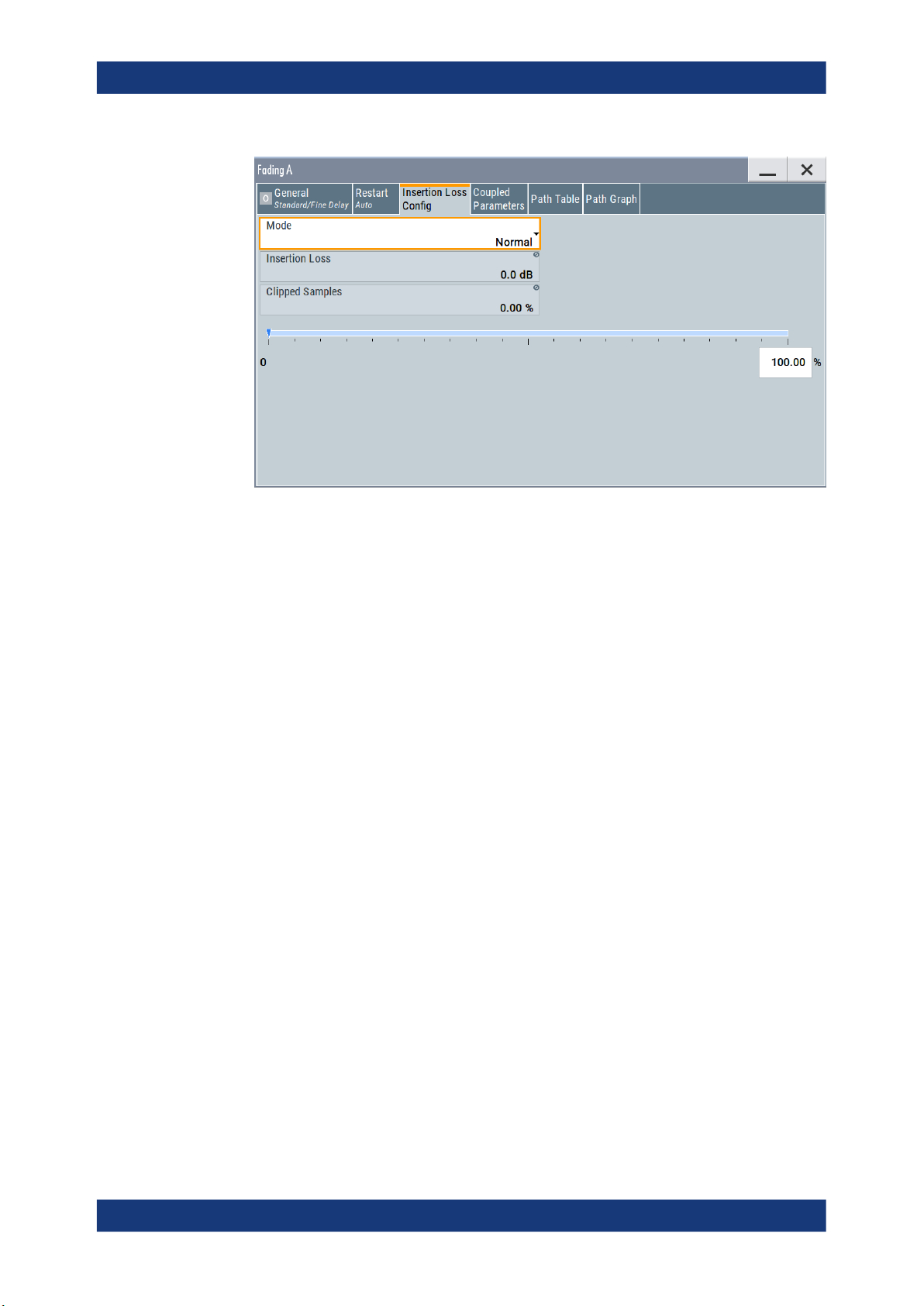
Fading settingsFading Simulation
Insertion loss configuration, coupled parameters and global fader coupling
Insertion Loss Mode......................................................................................................42
Insertion Loss................................................................................................................43
Clipped Samples...........................................................................................................43
0 ... 100 %.....................................................................................................................43
Insertion Loss Mode
Sets the mode for determining the insertion loss.
"Mode Normal"
"Mode Low ACP"
"Mode User"
Remote command:
[:SOURce<hw>]:FSIMulator:ILOSs:MODE on page 153
The insertion loss for a path of the fading simulator is automatically
chosen so that even when lognormal fading is switched on, overdrive
occurs only rarely in the fading simulator. This setting is recommended for bit error rate tests (BERTs). The current insertion loss is displayed under "Insertion Loss".
The insertion loss is automatically chosen so that an overdrive occurs
with an acceptable probability. "Low ACP" mode is only recommended for fading paths with Rayleigh profile as only in this case statistical distribution of level fluctuation is ensured. For other fading profiles, non-statistical level fluctuations occur which lead to an enormous increase of clipping. However, monitoring the percentage of
clipped samples is recommended for Rayleigh paths also.
The current insertion loss is displayed under "Insertion Loss".
Any value for the minimum insertion loss in the range from 0 dB to 18
dB can be selected. Desired value is entered under "Insertion Loss".
This mode is provided to ensure optimization of the dynamic range
and signal quality for any application. Display of the clipping rate for
any value which is entered enables estimation of the signal quality for
the specified signal dynamic range.
42User Manual 1175.6826.02 ─ 27

Fading settingsFading Simulation
Insertion loss configuration, coupled parameters and global fader coupling
Insertion Loss
Displays the current insertion loss in the "Normal" and "Low ACP" modes.
Entry of the insertion loss in "User" mode.
Remote command:
[:SOURce<hw>]:FSIMulator:ILOSs[:LOSS] on page 153
Clipped Samples
Displays the samples whose level is clipped as a %.
If the full drive level is reached for an insertion loss which is too low, the I/Q signals are
limited to the maximum available level (clipping).
Remote command:
[:SOURce<hw>]:FSIMulator:ILOSs:CSAMples? on page 153
0 ... 100 %
Graphically displays the samples whose level is clipped as a %. The scale resolution is
determined by entering the maximum value as a %.
3.3.2 Coupled parameters and global fader coupling settings
Access:
► Select "Fading > Insertion Loss Config/Coupled Parameters".
Coupled Parameters..................................................................................................... 44
└ Speed Setting Coupled...................................................................................44
└ Local Constant Coupled..................................................................................44
└ Standard Deviation Coupled...........................................................................44
Start Seed..................................................................................................................... 44
43User Manual 1175.6826.02 ─ 27

Fading settingsFading Simulation
Path table
Coupled Parameters
(available in "System Configuration > Mode > Standard")
Speed Setting Coupled ← Coupled Parameters
Sets the speed of the paths for both faders. The parameter Common Speed For All
Paths is also coupled.
Remote command:
[:SOURce<hw>]:FSIMulator:COUPle:SPEed on page 169
Local Constant Coupled ← Coupled Parameters
With lognormal fading, the parameter Local Constant is coupled for the paths of both
faders.
Remote command:
[:SOURce<hw>]:FSIMulator:COUPle:LOGNormal:LCONstant on page 168
Standard Deviation Coupled ← Coupled Parameters
With lognormal fading, the parameter Standard Deviation is coupled for the paths of
both faders.
Remote command:
[:SOURce<hw>]:FSIMulator:COUPle:LOGNormal:CSTD on page 168
Start Seed
Enters the start seed for random processes inside the fading simulator. This value is
global for the instrument but each fading path uses a different start seed. The autocorrelation of different seeds is more than seven days apart. If two instruments run with
the same seed, fading processes will be identical after a retrigger of the fading simulator.
While working in MIMO mode that requires two instruments, set the start seeds of the
instruments to different values.
Remote command:
[:SOURce<hw>]:FSIMulator:GLOBal:SEED on page 152
3.4 Path table
The settings for configuration of the fading paths are grouped in a path table.
1. To access this dialog, select "Fading > Fading Settings > Path Table".
The path table comprises the individual path and group parameters.
44User Manual 1175.6826.02 ─ 27

Fading settingsFading Simulation
Path table
Figure 3-3: Fading Path Table: Understanding the displayed information
1a/1b = Path group number (displayed in the first row) and path number (second row in the table
header); the example shows 4 groups with different number of active paths (the first group is
marked with a blue border)
2 = Fading profile, assigned per fading path
3/3a = Common group delay of a path group ("Basic Delay" is always 0 for group 1); adjustable for the
other groups (light grey background)
4 = Resulting delay per path, calculated as the sum of the common group delay and the path-spe-
cific delay
5 = Adjustable parameter for paths with Rice, WM Rice of Gauss Doppler fading
6 = Adjustable parameter for paths with Pure Doppler and constant Phase fading
7 = For moving receivers, selected speed ν or calculated as a function of the resulting Doppler shift
f
D
8 = Set resulting Doppler shift fD or calculated as fD=fRF*ν/c, where fRF is the selected RF and c the
speed of light
9 = Frequency ratio cosφt is ratio of the actual Doppler shift fA and the resulting Doppler shift f
10 = Actual Doppler shift fA calculated as fA=fD*cosφt
10 = Pure display parameters are on a dark background
11 = Access to a "Vector" or a "MIMO Matrix" for configuration of the correlation between the chan-
nels
2. To display all five paths per each group, change the settings as follows:
a) Select "Table Settings".
D
45User Manual 1175.6826.02 ─ 27

Fading settingsFading Simulation
b) In the "Path Table Settings" dialog, select "Path Filter > All Paths".
Cross-reference between the fading parameters
Consider the following interdependencies:
●
Delay parameters
Resulting Delay = Basic Delay + Additional Delay
●
Parameters influencing the Doppler shift calculation:
Resulting Doppler Shift fD calculated as:
fD = (ν/c)*fRF, where:
– ν is the Speed of the moving receiver
– fRF is the frequency of the RF output signal or the Virtual RF
–
c=2.998*108m/s is the speed of light
For "Fading Profile > Pure Doppler, Gauss Doppler or Rice", the Actual Doppler
Shift fA calculated as:
fA = fD*cosφt, where:
Path table
– cosφt is the Frequency Ratio and φ is the angle of incidence
–
fD is the Resulting Doppler Shift
3.4.1 Table settings
► To access this dialog, select "Fading > Fading Settings > Path Table > Table Set-
tings".
The provided functions facilitate settings configuration and navigation in the path
table, like suppression of the indication of disabled paths, quick change of the
speed unit.
Path Filter......................................................................................................................47
Speed Unit.................................................................................................................... 47
Keep Constant.............................................................................................................. 47
Common Speed For All Paths.......................................................................................47
46User Manual 1175.6826.02 ─ 27

Fading settingsFading Simulation
Path table
Path Filter
Suppresses the indication of the disabled paths.
Remote command:
n.a.
Speed Unit
Toggles between the available units for speed. The value always remains unchanged
but the display is automatically adapted to the selected unit.
Note: The remote control command changes only the units displayed in the graphical
user interface. While configuring the speed via remote control, the speed units must be
specified.
Remote command:
[:SOURce<hw>]:FSIMulator:SPEed:UNIT on page 159
Keep Constant
Selects whether to keep the speed or the resulting Doppler shift constant in case of frequency changes. If a constant speed is selected, the Doppler shift is calculated as
function of the speed and the frequency and vice versa.
Remote command:
[:SOURce<hw>]:FSIMulator:KCONstant on page 154
Common Speed For All Paths
In delay configurations, activates/deactivates the same speed in all paths.
If Speed Setting Coupled is enabled, this parameter is also coupled in both faders.
"On"
"Off"
Remote command:
[:SOURce<hw>]:FSIMulator:CSPeed on page 169
In this default state, a change of speed in a path automatically results
in a change of speed in all of the other paths.
When switching from "Off" to "On", the speed entry for path 1 of
group 1 is used for all of the paths.
3.4.2 Copy path group settings
The provided "Copy Path Group" settings enable you to copy the settings of one to a
second fading group.
Copy Path Group.......................................................................................................... 47
To.................................................................................................................................. 48
Copy..............................................................................................................................48
Copy Path Group
Selects a group whose settings are to be copied.
Remote command:
[:SOURce<hw>]:FSIMulator:COPY:SOURce on page 150
47User Manual 1175.6826.02 ─ 27

To
Selects a group whose setting is to be overwritten.
Remote command:
[:SOURce<hw>]:FSIMulator:COPY:DESTination on page 150
Copy
Triggers a copy procedure.
Remote command:
[:SOURce<hw>]:FSIMulator:COPY:EXECute on page 150
3.4.3 Path table settings
State Path..................................................................................................................... 48
Profile............................................................................................................................49
Path Loss...................................................................................................................... 50
Basic Delay................................................................................................................... 51
Additional Delay............................................................................................................ 51
Resulting Delay.............................................................................................................51
Power Ratio...................................................................................................................51
Frequency Spread.........................................................................................................51
Frequency Shift.............................................................................................................52
Const. Phase.................................................................................................................52
Start Phase................................................................................................................... 52
Speed............................................................................................................................52
Resulting Doppler Shift................................................................................................. 53
Frequency Ratio............................................................................................................53
Actual Doppler Shift...................................................................................................... 54
Correlation Path............................................................................................................ 54
Correlation Coefficient...................................................................................................55
Correlation Coefficient Phase........................................................................................55
Lognormal State............................................................................................................55
Local Constant.............................................................................................................. 55
Standard Deviation .......................................................................................................56
Fading settingsFading Simulation
Path table
State Path
Activates a fading path.
After activating, the fading process is initiated for this path with the selected fading pro-
file. However, the fading simulator must be switched on.
Remote command:
[:SOURce<hw>]:FSIMulator[:STATe] on page 167
[:SOURce<hw>]:FSIMulator:DELay|DEL:GROup<st>:PATH<ch>:STATe
on page 179
[:SOURce<hw>]:FSIMulator:MDELay:DEL30:GROup<st>:PATH<ch>:STATe
on page 179
[:SOURce<hw>]:FSIMulator:HSTRain:PATH:STATe on page 187
48User Manual 1175.6826.02 ─ 27

Fading settingsFading Simulation
Path table
Profile
Determines the fading profile for the selected path. The fading profile determines which
transmission path or which radio hop is simulated.
See also "Fading Profile" on page 24.
Depending on which profile is selected, certain parameters are available in the path
table and others are not available.
With correlated paths, the profile setting must agree. When correlation is activated, the
setting of the path for which correlation is switched on is accepted for both paths. Afterwards, the most recent modification applies to both paths (no matter in which path it
was made).
"Static Path"
"Pure Doppler"
"Rayleigh"
"Rice"
"Const. Phase"
"Gauss1"
Simulated is a static transmission path which can undergo attenuation (loss) or delay.
Simulated is a transmission path with an individual direct connection
from the transmitter to the moving receiver (discrete component).
The actual Doppler shift is determined by the Speed and Frequency
Ratio parameters.
Tip: In MIMO configuration, use the Relative gain vector matrix set-
tings to configure beamforming.
Simulated is a radio hop in which many highly scattered subwaves
arrive at a moving receiver.
Simulated is a radio hop in which a strong direct wave (discrete component) arrives at a moving receiver in addition to many highly scattered subwaves.
Use the parameter Power Ratio to set the ratio of the power of the
two components (Rayleigh and pure Doppler).
Simulated is one transmission path with the set constant phase rotation, attenuation (loss) or delay.
Option: R&S SMW-K72
Sum of two Gaussian functions and is used for excess delay times in
the following range:
0.5 µs to 2 µs, (0.5 µs < τI < 2 µs).
S(τI,f) = G(A, -0.8fd, 0.05fd) + G (A1, +0.4fd, 0.1fd)
where A1 is 10 dB below A.
"Gauss2"
"Gauss DAB"
Option: R&S SMW-K72
Sum of two Gaussian functions and is used for paths with delays in
excess of 2 µs, (τI > 2 µs).
S(τI,f) = G(B, +0.7fd, 0.1fd) + G (B1, -0.4fd, 0.15fd)
where B1 is 15 dB below B.
Option: R&S SMW-K72
Composed of a Gaussian function and is used for special DAB profiles.
S(τI,f) = G(A, ±0.7fd, 0.1fd)
where + 0.7fd applies for even path numbers and 0.7fd for odd, except
path 1.
49User Manual 1175.6826.02 ─ 27

"Gauss Doppler"
"Gauss (0.08 fd)"
"Gauss (0.1 fd)"
"Gauss (Watters)"
"WM Doppler"
Fading settingsFading Simulation
Path table
Option: R&S SMW-K72
Sum of a Gaussian function and a pure Doppler component.
S(τI,f) = G(0.1A; 0; 0.08fd) + δ(f-0.5fd)
Option: R&S SMW-K72
Composed of a Gaussian function with a standard deviation of
0.08*fd.
S(τI,f) = G(A; f; 0.08fd)
Option: R&S SMW-K72
Composed of a Gaussian function with a standard deviation of 0.1*fd.
S(τI,f) = G(A; f; 0.1fd)
Option: R&S SMW-K72
Gauss (Watterson) fading profile.
Option: R&S SMW-K72
The WiMAX Doppler fading profile is a rounded Doppler PSD model
according to IEEE 802.16a.
"WM Rice"
"Bell Shape tgn Indoor/Bell Shape tgn Moving Vehicle"
"SCM"
"Custom"
Remote command:
[:SOURce<hw>]:FSIMulator:DELay|DEL:GROup<st>:PATH<ch>:PROFile
on page 178
[:SOURce<hw>]:FSIMulator:MDELay:DEL30:GROup<st>:PATH<ch>:PROFile
on page 178
Option: R&S SMW-K72
The WiMAX Rice fading profile is according to IEEE 802.16a.
Both Bell Shape fading profiles describe the indoor wireless channels
according to IEEE 802.11n and IEEE 802.11ac.
The profiles are called after the resulting Doppler power spectrum
that has a shape very similar to a "Bell". The second fading profile
includes a Doppler component that represents a reflection from a
moving vehicle.
Option: R&S SMW-K73
The SCM profile is a geometry-based channel model that improves
the accuracy of the simulated channel model.
To access the settings, select "SCM Profile > SCM Data", see Chap-
ter 5.3.7, "SCM fading profile", on page 114
Option: R&S SMW-K72
Customized Doppler fading profile developed by Cohda-Wirless; the
profile describes the channels for testing of IEEE 802.11p signals.
To access the required settings, select "Custom", see Chapter 3.11,
"Custom fading profile", on page 85.
Path Loss
Enters the loss for the selected path.
50User Manual 1175.6826.02 ─ 27

Fading settingsFading Simulation
Path table
Remote command:
[:SOURce<hw>]:FSIMulator:DELay|DEL:GROup<st>:PATH<ch>:LOSS
on page 178
Basic Delay
Option: R&S SMW-B14
Sets the basic delay.
Within a path group, all of the paths are jointly delayed by this value.
The path delay is calculates as:
Resulting Delay = Basic Delay + Additional Delay
The "Basic Delay" for group 1 is always 0. Thus, for the paths in group 1, the "Resulting Delay" is equal to the "Additional Delay".
See also Chapter 2.4, "Major differences between R&S SMW-B14 and R&S SMW-
B15", on page 25.
Remote command:
[:SOURce<hw>]:FSIMulator:DELay|DEL:GROup<st>:PATH<ch>:BDELay
on page 171
Additional Delay
Sets the Additional Delay per path.
Remote command:
[:SOURce<hw>]:FSIMulator:DELay|DEL:GROup<st>:PATH<ch>:ADELay
on page 170
Resulting Delay
Displays the Resulting Delay for the path.
Remote command:
[:SOURce<hw>]:FSIMulator:DELay|DEL:GROup<st>:PATH<ch>:RDELay?
on page 171
Power Ratio
("Fading Profile > Rice, WM Rice, Gauss Doppler")
Enters the power ratio of the discrete component and distributed component.
The total power consisting of the two components is always constant. At a high power
ratio, the discrete (Doppler) component prevails. At a low power ratio, the distributed
(Rayleigh) component prevails.
Remote command:
[:SOURce<hw>]:FSIMulator:DELay|DEL:GROup<st>:PATH<ch>:PRATio
on page 178
Frequency Spread
("Fading Profile > Gauss Watterson")
Sets the frequency spread for the Gauss Watterson fading.
51User Manual 1175.6826.02 ─ 27

Fading settingsFading Simulation
Path table
Remote command:
[:SOURce<hw>]:FSIMulator:DELay|DEL:GROup<st>:PATH<ch>:FSPRead
on page 176
Frequency Shift
("Fading Profile > Gauss Watterson")
Enters the frequency shift for the Gauss Watterson fading.
Remote command:
[:SOURce<hw>]:FSIMulator:DELay|DEL:GROup<st>:PATH<ch>:FSHift
on page 176
Const. Phase
Enters the phase by which the path is multiplied.
Remote command:
[:SOURce<hw>]:FSIMulator:DELay|DEL:GROup<st>:PATH<ch>:CPHase
on page 173
Start Phase
("Fading Profile > Pure Doppler, WM Doppler")
A transmission path with the set start phase rotation is simulated which can undergo
attenuation (loss) or delay.
Remote command:
[:SOURce<hw>]:FSIMulator:DELay|DEL:GROup<st>:PATH<ch>:CPHase
on page 173
Speed
Enters the speed ν of the moving receiver.
The Resulting Doppler Shift fD is calculated as:
fD = (ν/c)*fRF, where
fRF is the frequency of the RF output signal or the virtual RF frequency and
c=2.998*108m/s is the speed of light
Example:
If ν = 100 km/h and fRF = 1 GHz, the fD = 92.66 Hz
Consider the following interdependencies:
●
If the speed is changed, the resulting Doppler shift is automatically modified.
●
If "Path Table Settings > Common Speed in All Paths > On", a change of speed in
one path automatically results in a change of speed in all of the other paths of the
fader.
●
In the "Fading Profile > Pure Doppler/Rice/Gauss Doppler", the actual Doppler
Shift fA is a function of the selected speed ν and also of the parameter Frequency
Ratio.
See also "Cross-reference between the fading parameters" on page 46
●
In "System Configuration > Mode > Standard", you can couple the speed for the
paths of both faders.
52User Manual 1175.6826.02 ─ 27

Fading settingsFading Simulation
Path table
●
With correlated paths, the speed setting must agree. When correlation is activated,
the settings of the path for which correlation is switched on are accepted for both
paths. Afterwards, the most recent modification applies to both paths (no matter in
which path it was made). The same applies to all paths of the two faders when
coupling is activated.
Remote command:
[:SOURce<hw>]:FSIMulator:DELay|DEL:GROup<st>:PATH<ch>:SPEed
on page 179
Resulting Doppler Shift
If "Table Settings > Keep Constant > Speed", this parameter displays the resulting
Doppler shift fD.
The value depends on the selected:
●
Speed
●
RF frequency fRF or the Virtual RF
●
For "Fading Profile > Pure, Gauss Doppler or Rice", the "Actual Doppler Shift"
depends also on the selected Frequency Ratio.
See "Cross-reference between the fading parameters" on page 46.
To set the Doppler shift, enable "Table Settings > Keep Constant > Resulting Doppler
Shift". In this case, the "Speed" is calculated as a function of the selected "Resulting
Doppler Shift" and the RF frequency fRF.
Remote command:
[:SOURce<hw>]:FSIMulator:DELay|DEL:GROup<st>:PATH<ch>:FDOPpler[:
RESulting] on page 174
Frequency Ratio
("Fading Profile > Pure, Gauss Doppler or Rice")
Sets the ratio of the actual Doppler Shift fA to the Resulting Doppler Shift fD.
The actual Doppler shift is a function of the simulated angle of incidence of the discrete
component (see Figure 3-4) and is calculated as:
fA = fD*cosφt, where:
cosφt is the "Frequency Ratio" and fD= (v/c)*fRF is the Resulting Doppler Shift.
Negative values indicate a receiver that is going away from the transmitter, and posi-
tive values a receiver that is approaching the transmitter.
53User Manual 1175.6826.02 ─ 27

Fading settingsFading Simulation
Path table
Figure 3-4: Doppler shift as a function of the angle of incidence
See also "Cross-reference between the fading parameters" on page 46
With correlated paths, the speed setting of the Frequency Ratio must agree. When cor-
relation is activated, the settings of the path for which correlation is switched on are
accepted for both paths. Afterwards, the most recent modification applies to both paths
(no matter in which path it was made).
Remote command:
[:SOURce<hw>]:FSIMulator:DELay|DEL:GROup<st>:PATH<ch>:FRATio
on page 175
Actual Doppler Shift
("Fading Profile > Pure Doppler, Gauss Doppler, Rice")
Displays the actual Doppler shift fA. The value depends on Frequency Ratio and
Resulting Doppler Shift.
See also "Cross-reference between the fading parameters" on page 46.
Remote command:
[:SOURce<hw>]:FSIMulator:DELay|DEL:GROup<st>:PATH<ch>:FDOPpler:
ACTual? on page 175
Correlation Path
Switches on correlation to the corresponding path of the second fader for dual-channel
fading.
Setting correlation necessitates synchronous signal processing on both channels. This
means the settings of the following parameters for the correlated fading paths must
agree:
●
"Profile"
●
"Speed"
●
"Frequency Ratio"
●
"Lognormal Parameters"
●
"Resulting Doppler Shift"
●
"Actual Doppler Shift"
When correlation is activated, the settings of the path for which correlation is switched
on are accepted for both paths. Afterwards, the most recent modification applies to
both paths (no matter in which path it was made).
54User Manual 1175.6826.02 ─ 27

Fading settingsFading Simulation
Path table
Correlated paths in dual-channel fading with the same input signal simulate the receiving conditions experienced by a receiver having two antennas in which the received
signals exhibit a certain degree of correlation due to a similar environment.
Remote command:
[:SOURce<hw>]:FSIMulator:DELay|DEL:GROup<st>:PATH<ch>:
CORRelation:STATe on page 173
Correlation Coefficient
Sets the magnitude of the complex correlation coefficient as a percentage.
The higher the entered percentage, the greater the correlation of the statistical fading
processes for the two correlated paths. Highly correlated ambient conditions for the
signal are simulated in this manner.
Each fader has a maximum of 20 paths.
With correlated paths, the coefficient setting must agree. When correlation is activated,
the setting of the path for which correlation is switched on is accepted for both paths.
Afterwards, the most recent modification applies to both paths (no matter in which path
it was made).
Remote command:
[:SOURce<hw>]:FSIMulator:DELay|DEL:GROup<st>:PATH<ch>:
CORRelation:COEFficient on page 172
Correlation Coefficient Phase
Sets the phase of the complex correlation coefficient in degrees.
With correlated paths, the coefficient phase setting must agree. When correlation is
activated, the setting of the path for which correlation is switched on is accepted for
both paths. Afterwards, the most recent modification applies to both paths (no matter in
which path it was made).
Remote command:
[:SOURce<hw>]:FSIMulator:DELay|DEL:GROup<st>:PATH<ch>:
CORRelation:PHASe on page 172
Lognormal State
Switches lognormal fading on/off (slow fading).
Simulated is an additional slow fluctuation of the received amplitude of a moving
receiver. This can occur due to peculiarities in the landscape or topography (e.g. when
driving through a depression). Lognormal fading has a multiplicative effect on the path
loss. The multiplication factor is time-variable and logarithmically normally distributed. If
a Rayleigh profile is set simultaneously, what we obtain is Suzuki fading.
Note: Since the slow level fluctuation is not taken into account statistically in the computation of the insertion loss, the output power can deviate from the displayed power.
Remote command:
[:SOURce<hw>]:FSIMulator:DELay|DEL:GROup<st>:PATH<ch>:LOGNormal:
STATe on page 177
Local Constant
Enters the Local Constant for lognormal fading.
55User Manual 1175.6826.02 ─ 27

Fading settingsFading Simulation
Path graph
The Local Constant L and the speed v of the moving receiver determine the limit frequency fL for lognormal fading:
fL = v/L.
The power density spectrum of an unmodulated carrier consists of a discrete spectral
line at fRF and a frequency-dependent continuous component for which the following
applies:
The lower setting limit is a function of the (virtual) RF frequency fRF and is calculated as
follows:
L
= 12*109 / f
min
RF
Remote command:
[:SOURce<hw>]:FSIMulator:DELay|DEL:GROup<st>:PATH<ch>:LOGNormal:
LCONstant on page 177
Standard Deviation
Enters the standard deviation in dB for lognormal fading.
Remote command:
[:SOURce<hw>]:FSIMulator:DELay|DEL:GROup<st>:PATH<ch>:LOGNormal:
CSTD on page 176
3.5 Path graph
To access the graphical representation of the configured path,
► select "Fading > Path Graph".
The path graph provides a quick overview of the paths as they are configured in
the delay modes.
56User Manual 1175.6826.02 ─ 27

Fading settingsFading Simulation
Birth death propagation
The signal delay is plotted on the x-axis. The minimum value is 0 s. The maximum
value is equal to the maximum delay, determined by the sum of max. Basic Delay and
max. Additional Delay. The relative path power is plotted on the y-axis, with 0 dB corre-
sponding to the maximum power on the path (path loss = 0 dB).
Each path is represented by a bar. The color of the bar indicates the fading profile of
the path. The color coding for the individual profiles is shown right next to the graphics.
The "Path Loss" can be read off from the height of the bar. The minimum value is 0 dB,
and the maximum value is – 50 dB.
3.6 Birth death propagation
In the "Birth Death Propagation" configuration, the fading simulator simulates dynamic
propagation conditions in conformity with the test case 3GPP, 25.104-xxx, annex B4.
Here, the behavior of a receiver is tested when it is confronted with the sudden disappearance and reappearance of a signal. This can occur, for example, when a pedestrian making a call walks around the corner of a building.
Two paths are simulated which appear ("Birth") or disappear ("Death") in alternation at
arbitrary points in time. The points in time fall within a grid of integer delays [-5, -4, -3,
-2, -1, 0, 1, 2, 3, 4, 5] µs. After a certain time ("Hopping Dwell"), a path disappears from
a given grid position and appears simultaneously at another randomly chosen grid
position. During this hop, the second path remains stable at its grid position. After a further "Hopping Dwell" elapses, the second path changes its position. Now, the first path
remains at its position and so on. The two paths never appear at the same time position at the same time (see Figure 3-5).
57User Manual 1175.6826.02 ─ 27

Fading settingsFading Simulation
Birth death propagation
Figure 3-5: Example of a sequence of hops in Birth Death Propagation
Since it is not possible to generate negative time values (delays), the actual hop range
is from 0 to 10 µs.
According to annex B4, each path has the same loss and phase and no Doppler shift.
The time until the position of a path is changed is also specified (see Table 3-2).
Table 3-2: Default parameter values (Birth Death Propagation)
"Profile" Pure Doppler
"Path Loss" 0 dB
"Min. Delay" 0 μs
"Delay Grid" 1 μs
"Positions" 11
"Max. Delay" 10 μs
"Hopping Dwell" 191 ms
"Speed" 0 m/s
"Frequency Ratio" 1.0
Path Graph
The graphical display of the fading paths in Birth Death Propagation mode shows as
an example the changing positions of the two paths within the delay grid. The displayed position change does not correspond to the actual delay hops of the real signal.
An arrow indicates the direction of the delay hop of the path that will next change its
position, with the head of the arrow marking the new position.
The delay grid is plotted on the x-axis. The permissible delay range and the delay offset are shown in the graphics (see the "Min Delay" and the "Delay Range" indication
on the graph). The path power is plotted on the y-axis, with 0 dB corresponding to the
maximum power on the path (path loss = 0 dB). The scaling of the axes and the displayed path power match the real settings.
The scaling of the x-axis depends on the set delay range. It always starts at 0 µs and
rages up to 40 µs at the most (= maximum for delay range). The minimum delay corresponds to the start value of the delay range. The maximum delay is defined by the minimum delay, the delay grid and the number of possible hop positions.
Max Delay = (Positions – 1) x Delay Grid + Min. Delay
58User Manual 1175.6826.02 ─ 27

Fading settingsFading Simulation
Birth death propagation
The (mean) delay offset is calculated from the minimum and maximum delay ((max.
delay - min. delay)/2).
The Table 3-2 lists the default values for Birth Death Propagation. However, these
parameters can also be set for further tests in the fading path table.
Settings:
Profile............................................................................................................................60
Path Loss...................................................................................................................... 60
Min Delay...................................................................................................................... 60
Delay Grid..................................................................................................................... 60
Positions........................................................................................................................60
Maximum Delay............................................................................................................ 61
59User Manual 1175.6826.02 ─ 27

Fading settingsFading Simulation
Birth death propagation
Start Offset....................................................................................................................61
Hopping Dwell...............................................................................................................61
Speed............................................................................................................................62
Resulting Doppler Shift................................................................................................. 62
Frequency Ratio............................................................................................................62
Actual Doppler Shift...................................................................................................... 63
Profile
Displays the fading profile for birth death propagation. The fading profile has a fixed
setting to "Pure Doppler".
A transmission path is simulated in which there is an individual direct connection from
the transmitter to the moving receiver (discrete component). The Doppler frequency
shift is determined by the "Speed" and "Frequency Ratio" parameters.
Remote command:
[:SOURce<hw>]:FSIMulator:BIRThdeath:PATH<ch>:PROFile on page 182
Path Loss
Enters the loss for the selected path.
Remote command:
[:SOURce<hw>]:FSIMulator:BIRThdeath:PATH<ch>:LOSS on page 182
Min Delay
Enters the minimum delay for the two fading paths.
The minimum delay corresponds to the start value of the delay range.
The delay range is defined by the minimum delay, the delay grid and the number of
possible hop positions. It can be in the range between 0 and 40 us.
0 us < (Positions – 1) x Delay Grid + Min. Delay < 40 us
The scaling of the X-axis is adapted according to the entry (see "Path Graph"
on page 58).
Invalid entries are rejected, the next possible value is entered.
Remote command:
[:SOURce<hw>]:FSIMulator:BIRThdeath:DELay:MINimum on page 181
Delay Grid
Enters the delay grid. The value defines the resolution for the possible hop positions of
the two fading paths in the delay range.
The scaling of the X-axis is adapted according to the entry (see "Path Graph"
on page 58).
Invalid entries are rejected, the next possible value is entered.
Remote command:
[:SOURce<hw>]:FSIMulator:BIRThdeath:DELay:GRID on page 180
Positions
Enters the number of possible hop positions in the delay range.
The scaling of the X-axis is adapted according to the entry (see "Path Graph"
on page 58).
60User Manual 1175.6826.02 ─ 27

Fading settingsFading Simulation
Birth death propagation
Invalid entries are rejected, the next possible value is entered.
Remote command:
[:SOURce<hw>]:FSIMulator:BIRThdeath:POSitions on page 182
Maximum Delay
Indication of the maximum delay. The maximum delay corresponds to the stop value of
the delay range (see "Path Graph" on page 58).
The maximum delay is defined by the minimum delay, the delay grid and the number of
possible hop positions.
Max Delay = (Positions – 1) x Delay Grid + Min. Delay
Remote command:
[:SOURce<hw>]:FSIMulator:BIRThdeath:DELay:MAXimum? on page 181
Start Offset
Enters the timing offset by which the start of "Birth Death Propagation" is offset with
respect to when fading is switched on or a restart as a result of a restart trigger.
This allows the user to precisely displace birth death events with respect to one
another during two-channel fading. This is required in some 3GPP base station tests.
If the same hopping dwell time is entered in both faders, the offset will take place by a
constant value.
Remote command:
[:SOURce<hw>]:FSIMulator:BIRThdeath:SOFFset on page 182
Hopping Dwell
Enters the time until the next change in the delay of a path (birth death event).
61User Manual 1175.6826.02 ─ 27

Fading settingsFading Simulation
Birth death propagation
During two-channel fading, the dwell times of the two channels can be set independently. This causes the hop time points of the two channels to coincide repeatedly. This
is a way of simulating tough receiving conditions as arise when two receiving channels
simultaneously change frequency (see figure).
Remote command:
[:SOURce<hw>]:FSIMulator:BIRThdeath:HOPPing:DWELl on page 181
Speed
Enters the speed v of the moving receiver.
The resulting Doppler shift is dependent on the speed v and the entered ratio of the
actual Doppler shift to the set Doppler shift fD. This ratio is determined in the "Frequency Ratio" line. The resulting Doppler frequency can be read off from the "Res.
Doppler Shift" line. It may not exceed the maximum Doppler frequency.
If the speed is changed, the resulting Doppler shift is automatically modified.
Remote command:
[:SOURce<hw>]:FSIMulator:BIRThdeath:SPEed on page 183
Resulting Doppler Shift
Displays the resulting Doppler shift.
Remote command:
[:SOURce<hw>]:FSIMulator:BIRThdeath:PATH<ch>:FDOPpler? on page 184
Frequency Ratio
Enters the ratio of the actual Doppler shift to the Doppler shift set with the "Speed"
parameter.
Remote command:
[:SOURce<hw>]:FSIMulator:BIRThdeath:FRATio on page 183
62User Manual 1175.6826.02 ─ 27

Actual Doppler Shift
Displays the actual Doppler shift.
The actual Doppler frequency is determined by the selected "Speed" and "Frequency
Ratio" (i.e. the ratio of the actual Doppler frequency to the resulting Doppler frequency).
Remote command:
[:SOURce<hw>]:FSIMulator:BIRThdeath:PATH<ch>:FDOPpler:ACTual?
on page 184
3.7 Moving propagation
In the "3GPP/LTE Moving Propagation" configuration, the fading simulator simulates
dynamic propagation conditions in conformity with the test case 3GPP TS25.104,
annex B3 or 3GPP TS36.141, annex B.4.
The fading simulator enables configuration according to three predefined moving scenarios. The first one represents moving conditions with one reference and one moving
channel whereas in the other two all paths are moving.
Fading settingsFading Simulation
Moving propagation
The predefined scenarios are as follow:
●
"Ref. + Mov. Channel" - Simulation of moving propagation conditions in accordance
to the 3GPP TS25.104, annex B3.
(see Chapter 3.7.1, "Moving propagation conditions for testing of baseband perfor-
mance", on page 63)
●
"ETU200Hz Moving" - Simulation of moving propagation conditions in accordance
to the scenario 1 described in 3GPP TS36.141, annex B.4.
(see Chapter 3.7.2, "Moving propagation conditions for testing the UL timing
adjustment performance", on page 66)
●
"Pure Doppler Moving" - Simulation of moving propagation conditions in accordance to the scenario 2 described in 3GPP TS36.141, annex B.4.
(see Chapter 3.7.2, "Moving propagation conditions for testing the UL timing
adjustment performance", on page 66)
It is also possible to adjust some of the parameters of these predefined scenarios and
simulate user-definable moving propagation conditions.
3.7.1 Moving propagation conditions for testing of baseband performance
Simulating moving propagation conditions for testing of baseband performance
► To simulate moving propagation conditions for testing of baseband performance in
accordance to the 3GPP TS25.104, annex B3:
a) select "Configuration > Moving Propagation" and "Moving Channels > One" or
b) select "Standard > 3GPP > Moving Propagation > Ref. + Mov. Channel".
63User Manual 1175.6826.02 ─ 27

Fading settingsFading Simulation
Moving propagation
Here, the behavior of a receiver is tested in response to slow delay variations in a signal. Two paths are simulated: Path 1 has fixed delay (Reference Path, P1), while the
delay of path 2 varies slowly in a sinusoidal fashion (Moving Path, P2). The two paths
have no fading profile. They have the same level, the same phase and no Doppler
shift.
The following figure illustrates a baseband signal with ASK modulation (only one 1 bit,
then many 0 bits) which was subjected to moving propagation. Path P1 remains still
while path P2 moves in time relative to it. As a result of the luminescence setting on
the oscilloscope, the way in which P2 wanders over time is clearly visible.
The graphical display of the fading paths in Moving Propagation mode shows as an
example the changing positions of the moving path with respect to the stationary reference path. The displayed position change does not correspond to the actual delay
changes of the real signal.
The delay grid is plotted on the x-axis. The permissible delay range for the moving path
is shown in the graphics by the horizontal arrow. The grey path indicates the set start
delay for the Moving Path. The path power is plotted on the y-axis, with 0 dB corresponding to the maximum power on the path (path loss = 0 dB). The scaling of the
axes and the displayed path power match the real settings.
64User Manual 1175.6826.02 ─ 27

Fading settingsFading Simulation
Moving propagation
The delay Δτ
of the moving path obeys the following equation:
one
Where the values relate to the values proposed in the test case 3GPP, 25.104xxx,
annex B3 as follows:
●
Variation (Peak-Peak) = A
●
Delay = B + A/2
●
Variation Period = 2π /Δ ω
The Table 3-3 list the settings required to attain the values proposed in the test case
3GPP TS25.104, annex B3.
Table 3-3: Default parameter values (Moving Propagation)
Reference Path: "Delay" 0 us
Moving Path: "Variation (Pk Pk)" 5 us
"Path Loss" 0 dB
"State" On
"Variation Period" 157 s
"Delay" 3.5 us
"Path Loss" 0 dB
"State" On
These default values can be changed in the Path Table dialog.
65User Manual 1175.6826.02 ─ 27

Fading settingsFading Simulation
Moving propagation
3.7.2 Moving propagation conditions for testing the UL timing adjustment performance
The purpose of the uplink timing adjustments testing is to verify whether the base station sends timing advance commands and whether the base station estimates appropriate the uplink transmission timing.
Simulating moving propagation conditions
To simulate moving propagation conditions for testing the UL timing adjustment performance in conformity with the test cases "Moving propagation conditions", as defined in
3GPP 36.141, annex B.4:
► Select "Standard > LTE > Moving Propagation > ETU200Hz Moving or Pure Dop-
pler Moving"
The Figure 3-6 illustrates the moving propagation conditions for the test of the UL timing adjustment performance.
Figure 3-6: Moving Propagation Conditions
Use the parameter "Additional Delay" to configure the relative timing among all paths.
The time difference between the reference timing and the first path is according to the
following equation:
The 3GPP specification defines the uplink timing adjustments requirements for normal
and extreme conditions. The following two scenarios for the testing of UL timing
advance are specified:
●
Scenario 1: ETU200 ("ETU200Hz Moving") is the scenario for testing in normal
conditions.
This scenario considers ETU channel model and UE speed of 120km/h.
●
Scenario 2: AWGN ("Pure Doppler Moving") is the extreme conditions optional scenario.
The scenario corresponds to AWGN channel model and UE speed of 350km/h.
66User Manual 1175.6826.02 ─ 27

Fading settingsFading Simulation
Moving propagation
The fading simulator generates the signals for these scenarios in according to the
parameters defined in the 3GPP specification (see table Table 3-4). However, the fad-
ing simulator also allows the re-configuration of some of the predefined values.
Table 3-4: Default parameter values
Parameter Scenario 1 Scenario 2
Channel Model ETU200Hz Moving Pure Doppler
UE speed 120 km/h 350 km/h
CP length Normal Normal
"Variation (Peak-Peak)" 10 μs 10 μs
Δω
"Variation Period" = 2π/Δω 157.1 s 48.3 s
3.7.2.1 Scenario 1
Here, the behavior of a moving receiver is tested, i.e. the simulated scenario represents a moving receiver that changes its distance to the base station. The Fading Simulator generates the signal as a sequence of complete cycles of approach towards to
the BS antenna and moving away from it.
Per default, three Rayleigh path groups with three paths each are simulated. All paths
move.
0.04 1/s 0.13 1/s
The path group 1 has a fixed delay ("Basic Delay = 0 s"); the "Basic Delay" of the other
two path groups can be configured. The relative timing among all paths is determined
by the parameter "Additional Delay".
The three path groups have the same phase and speed; the Doppler shift is calculated
as a function of the selected speed.
67User Manual 1175.6826.02 ─ 27

3.7.2.2 Scenario 2
One path without a fading profile (Pure Doppler) is simulated. The path has constant
level and constant speed.
3.7.3 Path tables moving propagation
The parameters available for configuration depend on the selected number of Moving
Channels, one or all.
3.7.3.1 One moving channel
► To access the settings for configuring the moving and the reference path for the
moving propagation with one moving channel, perform on of the following:
a) select "Fading > Standard > 3GPP > Ref. + Mov. Channel"
b) select "Fading > Configuration > Moving Propagation" and "Moving Channels >
One".
Fading settingsFading Simulation
Moving propagation
Settings:
Reference Path Settings............................................................................................... 69
└ State................................................................................................................69
└ Path Loss........................................................................................................69
└ Delay...............................................................................................................69
Moving Path Settings.................................................................................................... 69
└ State................................................................................................................69
└ Path Loss........................................................................................................69
68User Manual 1175.6826.02 ─ 27

Fading settingsFading Simulation
Moving propagation
└ Delay...............................................................................................................69
└ Variation (Peak-Peak)..................................................................................... 69
└ Variation Period...............................................................................................70
Reference Path Settings
The following settings are provided:
State ← Reference Path Settings
Activates reference path P1 for moving propagation.
Remote command:
[:SOURce<hw>]:FSIMulator:MDELay:REFerence:STATe on page 193
Path Loss ← Reference Path Settings
Enters the loss for the reference path.
Remote command:
[:SOURce<hw>]:FSIMulator:MDELay:REFerence:LOSS on page 193
Delay ← Reference Path Settings
Enters the delay for the reference path.
Remote command:
[:SOURce<hw>]:FSIMulator:MDELay:REFerence:DELay on page 193
Moving Path Settings
The following settings are provided:
State ← Moving Path Settings
Activates moving fading path P2 for moving propagation.
Remote command:
[:SOURce<hw>]:FSIMulator:MDELay:MOVing:STATe on page 192
Path Loss ← Moving Path Settings
Enters the loss for the moving fading path.
Remote command:
[:SOURce<hw>]:FSIMulator:MDELay:MOVing:LOSS on page 192
Delay ← Moving Path Settings
Enters the average delay for the moving fading path.
The delay of the moving path slowly varies sinusoidal within the set variation range
around this delay.
Remote command:
[:SOURce<hw>]:FSIMulator:MDELay:MOVing:DELay:MEAN on page 191
Variation (Peak-Peak) ← Moving Path Settings
Enters the range for the delay of the moving fading path for moving propagation. The
delay of the moving path slowly varies sinusoidal within this range around the set mean
delay.
69User Manual 1175.6826.02 ─ 27

Remote command:
[:SOURce<hw>]:FSIMulator:MDELay:MOVing:DELay:VARiation on page 191
Variation Period ← Moving Path Settings
Period duration for delay variation. A complete variation cycle is passed through in this
time.
Remote command:
[:SOURce<hw>]:FSIMulator:MDELay:MOVing:VPERiod on page 192
3.7.3.2 All moving channels
► To access the settings for configuring the moving path groups and their paths, per-
form one of the following:
a) select "Fading > Standard > LTE > Moving Propagation > ETU200Hz Moving"
b) select "Fading > Standard > LTE > Moving Propagation > Pure Doppler Mov-
ing"
c) select "Fading > Configuration > Moving Propagation" and "Moving Channels >
All".
Fading settingsFading Simulation
Moving propagation
The number and the parameters of the predefined paths depend on the selected
scenario.
The most parameters in the "Path Table" correspond to the parameters described in
Chapter 3.4, "Path table", on page 44.
70User Manual 1175.6826.02 ─ 27

Fading settingsFading Simulation
Two channel interferer
Settings:
Delay Variation (Peak-Peak)......................................................................................... 71
Variation Period.............................................................................................................71
Delay Variation (Peak-Peak)
Enters the range for the delay of the moving fading paths for moving propagation with
all moving channels. The delay of the moving path slowly varies sinusoidal within this
range around the set mean delay.
Remote command:
[:SOURce<hw>]:FSIMulator:MDELay:ALL:MOVing:DELay:VARiation
on page 190
Variation Period
Period duration for delay variation. A complete variation cycle is passed through in this
time.
Remote command:
[:SOURce<hw>]:FSIMulator:MDELay:ALL:MOVing:VPERiod on page 189
3.8 Two channel interferer
In the "2 Channel Interferer" configuration, the fading simulates dynamic propagation in
conformity with the test cases 5 and 6 from MediaFlo. Here, path 1 has a fixed delay
while the delay of path two either varies slowly in a sinusoidal way or appears in alternation at arbitrary points in time. Thus, 2 channel interferer fading can be considered
as a combination of birth death propagation fading and moving propagation fading. The
main difference is the broader range of propagation obtainable with 2 channel interferer fading.
Each of the fading profiles "Static Path", "Pure Doppler" and "Rayleigh" can be allocated to the two paths.
Predefined Setting
The Table 3-5 and Table 3-6 list the settings required to attain the values proposed in
the MediaFlo test case 5 and 6.
Table 3-5: Test Case 5
Reference Path: "Profile" Static Path
"Relative Delay" 10 us
"Average Power" -3 dB
"Fading Type" Rayleigh, 60 km/h
Moving Path: "Profile" Hopping
"Doppler Spectrum" Classic 6 dB
"Static Delay" 40 us
71User Manual 1175.6826.02 ─ 27

Fading settingsFading Simulation
Two channel interferer
Table 3-6: Test Case 6
Reference Path: "Profile" Static Path
Moving Path: "Profile" Sliding
"Relative Delay" 0/110 us
"Average Power" -3 dB
"Fading Type" Static
"Doppler Spectrum" N/A
"Dwell Time" 2.9 s
"Relative Delay" 100 us
"Average Power" -3 dB
"Fading Type" Static
"Doppler Spectrum" N/A
"Relative Delay" 0/200 us
"Average Power" -3 dB
Fading Type Rayleigh, 3 km/h
"Doppler Spectrum" Classic 6 dB
"Period" 160 s
How to use the provides settings and configure a 2 channel interfering signal
The following are two examples on how to configure a "2 Channel Interferer" conditions. See how to:
●
"To enable a hopped moving mode" on page 72
●
"To enable a sliding moving mode" on page 73
To enable a hopped moving mode
Enable a 2 channel interfering signal with the following settings:
1. Reference Path:
a) "Delay Min = 30 μs"
b) "Profile = Static Path"
c) "Path Loss = 0 dB"
2. Moving Path:
a) "Delay Min = 0 μs"
b) "Profile = Static Path"
c) "Path Loss = 0 dB"
d) "Delay Max = 100 μs"
e) "Moving Mode > Hopping"
3. Enable "Reference Path > State > On" and "Moving Path > State > On"
72User Manual 1175.6826.02 ─ 27

4. Open the "Fading > Path Graph" view.
The following figure shows the resulting path graph.
Fading settingsFading Simulation
Two channel interferer
To enable a sliding moving mode
1. Use the settings of "To enable a hopped moving mode" on page 72.
2. Change the "Moving Mode > Sliding".
3. Open the "Fading > Path Graph" view.
The moving path slides from the minimum delay (30 us) to the maximum delay
(100 us) and back. The grey bar indicates the mean delay of the moving path. The
horizontal arrow indicates the permissible delay range for the moving path.
The displayed position change does not correspond to the actual delay changes of
the real signal.
73User Manual 1175.6826.02 ─ 27

Fading settingsFading Simulation
Two channel interferer
2 Channel Interferer Settings
The Table 3-5 and Table 3-6 list the default values for "2 Channel Interferer" configura-
tion. You can use these default values and/or adjust the provided settings in the fading
path table.
Settings:
State..............................................................................................................................74
Profile............................................................................................................................75
Path Loss...................................................................................................................... 75
Speed............................................................................................................................75
Freq. Ratio.................................................................................................................... 75
Res. Doppler Shift.........................................................................................................75
Act. Doppler Shift.......................................................................................................... 76
Delay Min...................................................................................................................... 76
Delay Max (Moving Path)..............................................................................................76
Moving Mode (Moving Path)......................................................................................... 76
Period/Dwell..................................................................................................................76
State
Activates/deactivates either the reference path or the moving path for 2 channel interferer fading.
74User Manual 1175.6826.02 ─ 27

Fading settingsFading Simulation
Two channel interferer
Remote command:
[:SOURce<hw>]:FSIMulator:TCINterferer[:STATe] on page 216
[:SOURce<hw>]:FSIMulator:TCINterferer:REFerence|MOVing:STATe
on page 219
Profile
Selects the fading profile either for the reference path or the moving path to be used for
2 channel interferer fading.
Remote command:
[:SOURce<hw>]:FSIMulator:TCINterferer:REFerence|MOVing:FDOPpler?
on page 218
Path Loss
Sets the attenuation of either the reference path or moving path to be used for 2 channel interferer fading.
Remote command:
[:SOURce<hw>]:FSIMulator:TCINterferer:REFerence|MOVing:LOSS
on page 219
Speed
(Rayleigh only)
Enters the speed v of the moving receiver. The unit for entering the speed under
"Speed Unit" can be chosen in the upper section of the menu.
The resulting Doppler shift is dependent on the speed v and the entered ratio of the
actual Doppler shift to the set Doppler shift fD. This ratio is determined in the "Frequency Ratio" line. The resulting Doppler frequency can be read off from the "Res.
Doppler Shift" line. It may not exceed the maximum Doppler frequency.
If the speed is changed, the resulting Doppler shift is automatically modified.
Remote command:
[:SOURce<hw>]:FSIMulator:TCINterferer:SPEed on page 217
Freq. Ratio
Enters the ratio of the actual Doppler shift to the Doppler shift set with the "Speed"
parameter.
Remote command:
[:SOURce<hw>]:FSIMulator:TCINterferer:REFerence|MOVing:FRATio
on page 218
Res. Doppler Shift
Displays the actual Doppler shift.
The actual Doppler frequency is determined by the entered "Speed" and the entered
ratio of the actual Doppler frequency to the set Doppler frequency ("Frequency Ratio").
Remote command:
[:SOURce<hw>]:FSIMulator:TCINterferer:REFerence|MOVing:FDOPpler?
on page 218
75User Manual 1175.6826.02 ─ 27

Fading settingsFading Simulation
Two channel interferer
Act. Doppler Shift
Displays the actual Doppler shift.
Remote command:
[:SOURce<hw>]:FSIMulator:TCINterferer:REFerence|MOVing:FDOPpler:
ACTual? on page 218
Delay Min
Enters the minimum delay for either the reference path or the moving path.
The minimum delay of the moving path corresponds to the start value of the delay
range.
The delay range is defined by the minimum delay and the maximum delay.
The scaling of the x-axis is adapted according to the entry.
Invalid entries are rejected, the next possible value is entered.
Remote command:
[:SOURce<hw>]:FSIMulator:TCINterferer:REFerence|MOVing:DELay:
MINimum on page 217
Delay Max (Moving Path)
Enters the maximum delay for the moving path.
The maximum delay of the moving path corresponds to the end value of the delay
range.
The delay range is defined by the minimum delay and the maximum delay.
The scaling of the x-axis is adapted according to the entry.
Invalid entries are rejected, the next possible value is entered.
Remote command:
[:SOURce<hw>]:FSIMulator:TCINterferer:REFerence|MOVing:DELay:
MAXimum on page 216
Moving Mode (Moving Path)
Selects the Type of moving applied to the moving path.
"Sliding"
"Hopping"
Remote command:
[:SOURce<hw>]:FSIMulator:TCINterferer:REFerence|MOVing:MMODe
on page 216
The reference path has a fix delay while the delay of the moving path
varies slowly in a sinusoidal way.
The reference path has a fix delay while the delay of the moving path
appears or disappears in alternation at arbitrary points in time.
Period/Dwell
Enters either the dwell time or the period of a complete cycle for the moving path
depending on the selected Moving Mode (Moving Path).
76User Manual 1175.6826.02 ─ 27

Fading settingsFading Simulation
Customized dynamic fading
"Moving Mode" "Period Dwell"
"Sliding" sets the period for a complete cycle of the moving path
"Hopping" sets the dwell time of the moving path
The gradient of the delay/period ratio may not fall below 6μs/s, that is, the minimum
value of the period depends on the value of the delay.
If the value for the delay is increased in a way that the value for the gradient falls below
6μs/s, the value for the period is recalculated automatically.
Example:
"Delay Min" = 20 us, "Delay Max" = 120 us, "Moving Mode = Sliding"
[("Delay max" - "Delay min")/2]*2π)/"Period/Dwell" = 6
"Period/Dwell" = 314/6 = 52.36 s
The value cannot be decreased below this value.
Remote command:
[:SOURce<hw>]:FSIMulator:TCINterferer:PERiod on page 217
3.9 Customized dynamic fading
Customized dynamic fading (CDF) allows you to import dynamic fading list files and to
vary the fading parameters path loss, Doppler shift and delay over time. This functionality requires option R&S SMW-K820
Customized dynamic fading is a suitable solution in the following cases:
●
If advanced dynamic fading models like the customized high-speed train scenarios
(cHST) are required
●
If a simulation based on measured real-world channel conditions is required
Such requirements are for example the UE tests in the context of performance
analysis.
Customized dynamic fading is available in SISO and MIMO configurations. This fading
configuration consists of up to 12 fading paths that can be activated individually. All
fading paths use rayleigh fading profile but a pure Doppler profile can also be assigned
to the first four paths.
The dynamic fading list files are application-specific list files in a Rohde & Schwarz proprietary file format and with the predefined file extension *.fad_udyn. Such files can
originate for example from drive test measurements. These measurement results have
to be converted in the required file format.
Access:
1. Select "Fading > General Setting > Configuration > Customized Dynamic"
2. Select "Path Table".
77User Manual 1175.6826.02 ─ 27

Customized dynamic fading
Up to 12 fading paths can be configured.
The displayed settings depend on the configuration (SISO or MIMO).
3. To load a fading list file, select "Filename > Select Predefined File".
Select on of the predefined files, e.g. Urban_Pure Doppler.
Fading settingsFading Simulation
Settings:
State..............................................................................................................................78
Profile............................................................................................................................78
Filename....................................................................................................................... 78
Correlation.....................................................................................................................79
State
If a fading list file is loaded, this parameter activates the path.
Each change of the state of a path causes a restart of the fader and therefore a restart
of all dynamic lists.
Remote command:
[:SOURce<hw>]:FSIMulator:CDYNamic:PATH<ch>:STATe on page 236
Profile
Sets the used profile. Per default, all fading paths use Rayleigh profile.
"Static Path"
"Pure Doppler"
"Rayleigh"
Remote command:
[:SOURce<hw>]:FSIMulator:CDYNamic:PATH<ch>:PROF on page 235
Fading profile for all paths
Fading profile for paths 1 to 4
Fading profile for all paths
Filename
You can load predefined or user-defined application-specific fading list files.
The fading list files are files in a Rohde & Schwarz proprietary file format and with the
predefined file extension *.fad_udyn.
78User Manual 1175.6826.02 ─ 27

Fading settingsFading Simulation
High-speed train
Such files can originate for example from drive test measurements. These measurement results have to be converted in the required file format.
Remote command:
[:SOURce<hw>]:FSIMulator:CDYNamic:CATalog? on page 234
[:SOURce<hw>]:FSIMulator:CDYNamic:CATalog:USER? on page 234
[:SOURce<hw>]:FSIMulator:CDYNamic:PATH<ch>:DATA:DSELect
on page 235
[:SOURce<hw>]:FSIMulator:CDYNamic:DELete on page 235
Correlation
In MIMO configurations, access dialogs to configure the correlation settings:
"Vector"
"Matrix"
For the "Pure Doppler" paths, opens the "Relative Tap Gain Vector"
dialog where you can configure the phase shift of the selected path.
For description, see Chapter 5.3.3, "Relative gain vector matrix set-
tings", on page 104.
For the "Rayleigh" paths, opens the "Correlation Matrix" dialog.
Available is only the "Matrix Mode > Individual", see Chapter 5.3.2,
"Correlation matrix table", on page 102.
3.10 High-speed train
In the "High Speed Train" configuration, the fading simulator simulates propagation
conditions in conformity with the test case "High-speed train conditions", as defined in
3GPP TS 25.141, annex D.4A and 3GPP TS 36.141, annex B.3. Here, the behavior of
a receiver in high-speed train conditions is tested, i.e. the simulated scenario represents a fast moving receiver that drives past an antenna. The fading simulator generates the signal as a seq uence of complete cycles of approach towards to the BS
antenna and departure from it.
Figure 3-7: High-speed train propagation
Three high-speed scenarios are defined:
●
Scenario 1: Open space
●
Scenario 2: Tunnel with leaky cable
●
Scenario 3: Tunnel for multi-antennas
79User Manual 1175.6826.02 ─ 27

3.10.1 Scenario 1 and scenario 3
For each of the scenarios 1 and 3, one path without a fading profile is simulated (Pure
Doppler). The path has constant level, no delay and variable Doppler shift.
The Doppler shift for these scenarios is calculated as follows:
Where fA(t) is the actual Doppler shift and fD is the maximum Doppler frequency.
The cosine of angle is given by:
Where:
●
DS/2 is the distance in meters between the train and the BS at the beginning of the
simulation
●
D
is the minimum distance in meters between the BS and the railway track
min
●
v is the velocity of the train in m/s
●
t is time in seconds
Fading settingsFading Simulation
High-speed train
For scenario 1 and for BS with receiver diversity, the Doppler shift variation is the same
between the antennas.
3.10.2 Scenario 2
Scenario 2 is not defined for EUTRA/LTE test cases.
For scenario 2, one Rician fading propagation channel with Rician factor K=10 dB and
with one tap is simulated. The Rician factor K is defined as the ratio between the dominant signal power and the variant of the other weaker signals (see "K (Rician factor)"
on page 84).
3.10.3 High-speed train scenario parameters
The Table 3-7 gives an overview of the parameters of the HST test scenarios accord-
ing to the test case "High-speed train conditions".
Table 3-7: Parameters for high-speed train conditions
Parameter
D
S
Scenario 1 Scenario 2 Scenario 3
1000 m Infinity 300 m
Value
D
min
K - 10 dB -
50 m - 2 m
80User Manual 1175.6826.02 ─ 27

Fading settingsFading Simulation
High-speed train
Parameter
v
f
D
350 km/h 300 km/h 300 km/h
1340 Hz 1150 Hz 1150 Hz
Value
The Figure 3-8 and Figure 3-9 show the trajectory of the Doppler shift for scenario 1
and 3 for the test parameters specified in the test case. For these two scenarios, the
Doppler shift trajectories for any user-defined parameters are also displayed in the
"3GPP HST" dialog.
Figure 3-8: Doppler shift trajectory for scenario 1
Figure 3-9: Doppler shift trajectory for scenario 3
Doppler shift calculation
The HST scenarios are defined for the UE and for the BS tests. In the fading simulator,
the same standards are used for both test cases. Consider however, the following difference in the calculation of the Doppler shift:
●
In HST UE tests, the resulting Doppler shift is based only on the used DL frequency.
●
In HST BS tests, the DL signal itself already contains a Doppler shift. The UE synchronizes on this shifted DL frequency. The simulated UL signal contains a Doppler
shift, too.
81User Manual 1175.6826.02 ─ 27

Fading settingsFading Simulation
High-speed train
The resulting Doppler shift is then based on both, the UL and the DL frequency.
To enable the fading simulator to consider the DL Doppler shift, use the following two
parameters:
●
Consider DL RF
●
Virtual DL RF
General recommendations on performing HST BS tests
The following is a list of the general steps required to enable the fading simulator to
generate the signal required for the HST BS tests
1. Set the "RF Frequency" of the instrument to the FUL, as defined in the specification.
2. Enable a high-speed train scenario with extension "(DL+UL)" in its name.
3. If not enabled, activate the parameter "Fading > (HST) Path Table > Consider DL
RF > On".
4. Set the value of the parameter "Fading > (HST) Path Table > Virtual DL RF" to the
FDL, as defined in the specification.
Example: Configuring the fading simulator to generate an HST BS test signal
according to 3GPP TS 36.104
For frequency band 1 tests, the specification defines: FDL = 2.14 GHz and FUL = 1.95
GHz. The resulting Doppler shift is FD = 1140 Hz.
●
In the status bar, select "Frequency = FUL = 1.95 GHz"
●
Select "Fading A > Fading Settings > Standards" and navigate to the required highspeed train scenario "3GPP > High Speed Train > HST 3 Tunnel Multi Antenna (DL
+UL)"
●
If not enabled, activate the parameter "Fading > Path Table > Consider DL RF >
On".
●
Select "Fading > Path Table > Virtual DL RF = FDL = 2.14 GHz"
●
Select "Fading > Fading Settings > State > On"
●
Use the command [:SOURce<hw>]:FSIMulator:HSTRain:FDOPpler? to
query the resulting Doppler shift.
Compare the example below and the Doppler shift trajectory specified in the 3GPP
TS36.104.
High-speed train scenario settings
To access these settings:
1. Select "Fading > Fading Settings > Standards".
2. Navigate to the required high-speed train scenario, e.g. "3GPP > High Speed Train
> HST 3 Tunnel Multi Antenna (DL+UL)"
The "3GPP HST" dialog displays the default values of the high-speed train scenarios and allows you to adjust them for further tests.
82User Manual 1175.6826.02 ─ 27

Settings:
Fading settingsFading Simulation
High-speed train
State..............................................................................................................................83
Profile............................................................................................................................83
Speed............................................................................................................................84
D (min).......................................................................................................................... 84
D (S)..............................................................................................................................84
K (Rician factor)............................................................................................................ 84
Consider DL RF............................................................................................................ 84
Start Offset....................................................................................................................85
Virtual DL RF.................................................................................................................85
State
Activates/deactivates simulation of high-speed train propagation according to the
selected scenario.
Remote command:
[:SOURce<hw>]:FSIMulator:HSTRain:STATe on page 189
Profile
Determines the fading profile for the selected scenario. The fading profile determines
which transmission path is simulated.
Although both scenarios 1 and 3 are specified as pure Doppler paths without a fading
profile and scenario 2 as a Rician fading, in this fading simulator you can change the
fading profile.
"Static Path"
A static transmission path with no attenuation (loss) or delay is simulated.
83User Manual 1175.6826.02 ─ 27

Fading settingsFading Simulation
High-speed train
"Pure Doppler"
A transmission path is simulated in which there is an individual direct
connection from the transmitter to the moving receiver (discrete component).
The simulated path has a constant delay and attenuation (no loss).
The Doppler frequency shift is determined only by the parameters
Speed, D (min) and D (S).
Tip: Use the SCPI command [:SOURce<hw>]:FSIMulator:
HSTRain:FDOPpler? to query the Doppler frequency shift.
"Rayleigh"
A radio hop is simulated in which many highly scattered subwaves
arrive at a moving receiver.
"Rice"
One Rician fading propagation channel with K (Rician factor) and with
one tap is simulated.
Remote command:
[:SOURce<hw>]:FSIMulator:HSTRain:PROFile on page 187
Speed
Sets the velocity parameter, i.e. the speed of the moving receiver.
Remote command:
[:SOURce<hw>]:FSIMulator:HSTRain:SPEed on page 186
D (min)
For "Profile > Static Path or Pure Doppler", sets the parameter D
to define the dis-
min
tance between the BS and the railway track.
Remote command:
[:SOURce<hw>]:FSIMulator:HSTRain:DISTance:MINimum on page 185
D (S)
For "Profile > Static Path or Pure Doppler", sets the parameter DS and define the initial
distance DS/2 between the train and the BS at the beginning of the simulation.
Remote command:
[:SOURce<hw>]:FSIMulator:HSTRain:DISTance:STARt on page 186
K (Rician factor)
For scenario 2, sets the Rician factor K that is defined as the ratio between the dominant signal power and the variant of the other weaker signals.
Remote command:
[:SOURce<hw>]:FSIMulator:HSTRain:KFACtor on page 187
Consider DL RF
Enables the selection of virtual downlink frequency (DL RF).
By default, this parameter is enabled for the HST (DL+UL) standards. For detailed
description, see "Doppler shift calculation" on page 81.
Note: While performing HST BS tests and "Consider DL RF > Off", the DL Doppler
shift is not considered by the calculation of the UL Doppler shift.
84User Manual 1175.6826.02 ─ 27

Fading settingsFading Simulation
Custom fading profile
Remote command:
[:SOURce<hw>]:FSIMulator:HSTRain:DOWNlink:FREQuency:STATe
on page 188
Start Offset
Set a value greater than zero to shift the HST profile in time.
Remote command:
[:SOURce<hw>]:FSIMulator:HSTRain:SOFFset on page 188
Virtual DL RF
Sets the virtual downlink frequency. For HST BS tests, enter the FDL defined in the
specification. The value is used by the calculation of the UL Doppler shift.
For detailed description, see "Doppler shift calculation" on page 81
Remote command:
[:SOURce<hw>]:FSIMulator:HSTRain:DOWNlink:FREQuency on page 188
3.11 Custom fading profile
The custom fading profile requires R&S SMW-K72.
The custom fading profile allows you to modify the classical Jakes and Flat fading profiles. These modified profiles are required by the IEEE 802.11p channel models.
A frequency offset f
cut-off frequencies, fl (lower) and fu (upper), can be configured to set the lower and
upper cut-off frequencies of the resulting spectrum, see Figure 3-10.
can be applied to shift the spectrum of the original profile. Two
offset
Figure 3-10: Resulting asymmetric Doppler spectrum
In the fading simulator, all these required profile parameters are configurable, see
"Custom fading profile settings" on page 86.
85User Manual 1175.6826.02 ─ 27

Custom fading profile settings
To access these settings:
1. Select "Fading > Fading Settings > Path Table"
2. Select "Profile > Custom"
3. Select "Custom Profile > Custom Data"
Fading settingsFading Simulation
Custom fading profile
Settings:
Doppler Shape.............................................................................................................. 86
Bandwidth..................................................................................................................... 86
Frequency Offset...........................................................................................................87
Lower/Upper Cutoff Frequency.....................................................................................87
Doppler Shape
Sets the Doppler shape ("Flat" or "Rayleigh") of the virtual profile.
Remote command:
[:SOURce<hw>]:FSIMulator:DELay|DEL:GROup<st>:PATH<ch>:CUSTom:
DSHape on page 220
Bandwidth
Sets the bandwidth of the original Doppler profile from which the resulting profile is created, see Figure 3-10.
86User Manual 1175.6826.02 ─ 27

Fading settingsFading Simulation
Custom fading profile
Remote command:
[:SOURce<hw>]:FSIMulator:DELay|DEL:GROup<st>:PATH<ch>:CUSTom:
DATA on page 220
Frequency Offset
Sets the frequency offset f
used to shift the original profile, see Figure 3-10.
offset
Remote command:
[:SOURce<hw>]:FSIMulator:DELay|DEL:GROup<st>:PATH<ch>:CUSTom:
DATA on page 220
Lower/Upper Cutoff Frequency
Sets the lower and upper cut-off frequencies, fl and fu, that depend on the original profile bandwidth Bandwidth.
The following applies:
●
f
≤
f
u
●
fl
≥
●
f
- f
u
●
50 Hz ≤ Bandwidth ≥ 40 kHz
+ Bandwidth/2
offset
f
-
Bandwidth/2
offset
≥ 1
Hz
l
Where the highest possible absolute cut-off frequency is 4 kHz.
Remote command:
[:SOURce<hw>]:FSIMulator:DELay|DEL:GROup<st>:PATH<ch>:CUSTom:
DATA on page 220
87User Manual 1175.6826.02 ─ 27
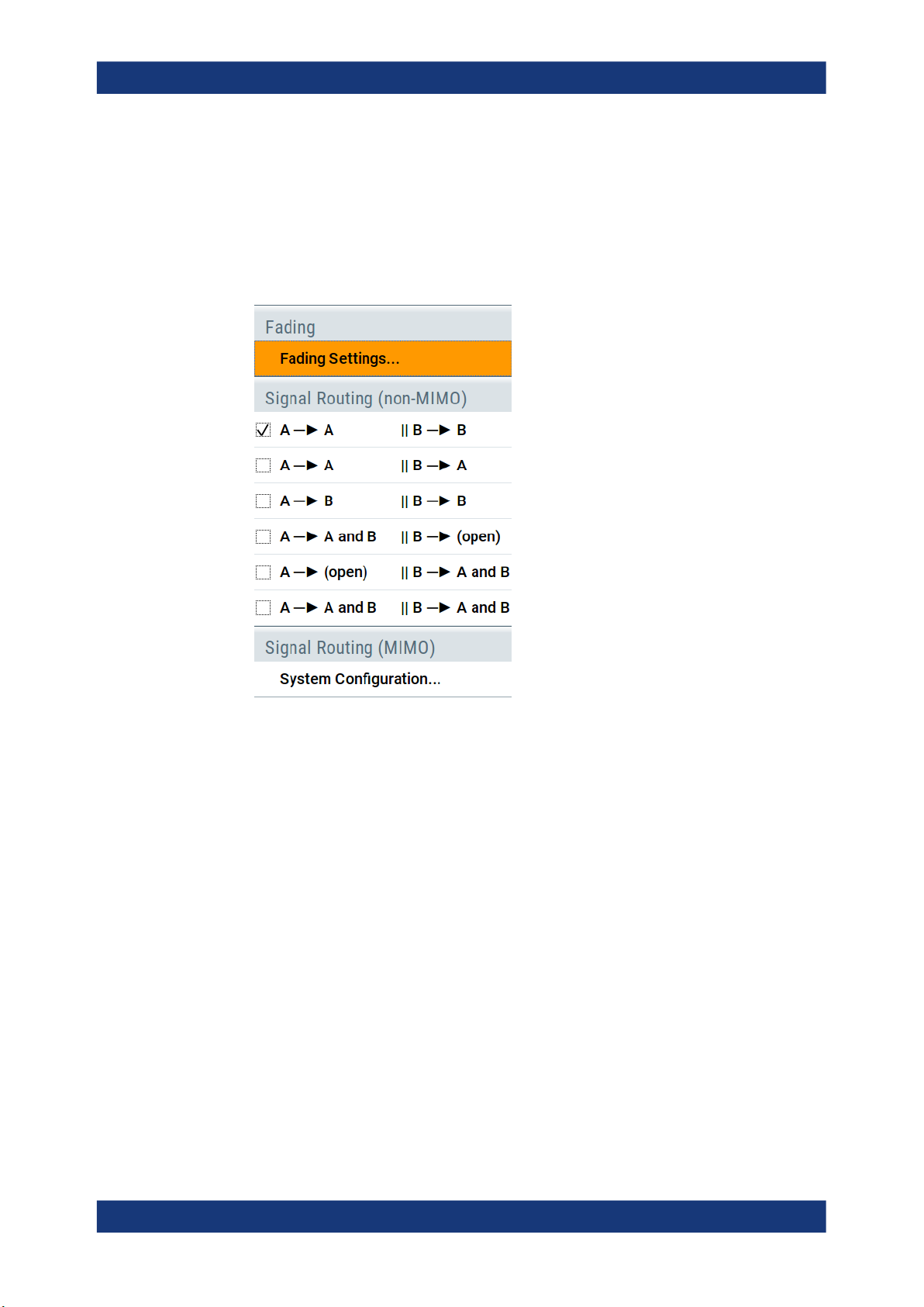
4 Signal routing settings
To route the signal in standard (non-MIMO) configuration
1. Select "System Configuration > Mode > Standard".
2. Select "Fading > Signal Routing (non-MIMO)".
Signal routing settingsFading Simulation
To route the signal in MIMO configuration
Option: R&S SMW-B14/-B15/-K74 and optionally R&S SMW-K75/-K76
► Follow the instructions in Chapter 5.2, "How to enable LxMxN MIMO test configura-
tions", on page 93.
To generate SISO signal with 400 MHz or 800 MHz fading bandwidth
Option: R&S SMW-B15/-K822/-K823
► Select SISO configuration by following the instructions in:
● "To enable MIMO configuration with 400 MHz fading bandwidth" on page 95.
● "To enable MIMO configuration with 800 MHz fading bandwidth" on page 96.
This section describes the settings related to the fading bandwidth and simulation.
For comprehensive description of all settings in the "System Configuration" dialog and
information on how to define the I/Q stream-mapping, connect external instruments,
etc.:
See section "Signal routing and system configuration" in the R&S SMW user manual.
88User Manual 1175.6826.02 ─ 27

Signal routing settingsFading Simulation
BB Bandwidth................................................................................................................89
CA Bandwidth............................................................................................................... 89
Signal Routing...............................................................................................................89
BB Bandwidth
Option: R&S SMW-B15/-K822/-K823
Sets the baseband signal bandwidth, that is supported by the fading simulator.
The value range and the maximal available bandwidth depend on the installed options
and the selected MIMO configuration.
For example:
●
In MIMO configurations with fewer than 8 channels, the max. baseband bandwidth
is 400 MHz.
●
In MIMO configurations with fewer than 4 channels, the max. baseband bandwidth
is 800 MHz.
For more information, see data sheet.
Remote command:
:SCONfiguration:BBBW on page 236
CA Bandwidth
Option: R&S SMW-B15/-K822/-K823
Indicates the resulting channel aggregation (CA) bandwidth, calculated based on the
MIMO configuration and the "BB Bandwidth".
The "CA Bandwidth" represents the signal bandwidth at the stream mapper.
For more information, see data sheet.
Remote command:
:SCONfiguration:CABW? on page 237
Signal Routing
In "System Configuration > Mode > Standard", defines the signal routing for the fading
signal at the output of the fading simulator.
Note: Signal routing for MIMO setups is performed with the settigns in the "System
Configuration" dialog, see Chapter 5.2, "How to enable LxMxN MIMO test configura-
tions", on page 93.
In remote control, however, all available signal routing settings are configured with the
command [:SOURce<hw>]:FSIMulator:ROUTe.
In "System Configuration > Mode > Standard", the input signal of the fading simulator
is defined by the setting "Baseband > Signal Routing". An instrument equipped with
two fading simulators and two baseband blocks, the input signal of each of the fading
simulator can be:
●
the signal from a single baseband block,
●
the summation signal from both baseband blocks or
●
each a signal from one of the two baseband blocks.
The following is a list of the routing settings for an instrument equipped with two base-
band blocks, two signal paths and two options fading simulator (R&S SMW-B14).
89User Manual 1175.6826.02 ─ 27

Signal routing settingsFading Simulation
"A to A/ B to B"
"A to A/B to A"
"A to B / B to B"
"A to A and B / B to A and B"
"A to A and B / B (open)"
Dual-channel fading. The fading signal from fader A is output on
baseband path A and the fading signal from fader B is output on
baseband path B.
The R&S SMW can be operated like two instruments; two independently configured signals are routed to the instrument's output.
This configuration is also suitable for transmit or receive diversity
tests:
●
Use the signal of one of the baseband generators to simulate the
receiving conditions of a receiver with two antennas, like a highquality car radio or UMTS base station.
●
Correlate the paths of the two fading simulators, i.e. the two fading channels. You can simulate the conditions of receiver with two
antennas which receive statistically correlated signals. Such condition appears, e.g., in a car with two antennas when the two
received signals exhibit a degree of correlation due to a similar
environment, like an underpass or hills.
Dual-channel fading. The fading signal from fader A and the fading
signal from fader B are both output on baseband path A.
This configuration is suitable for the simulation of:
●
mobile radio network handover in the handheld device
●
testing of filtering out the own signal if there is simultaneous presence of a strong signal from another standard.
To simulate the required conditions, configure each of the baseband
signals according to the desired standard and route them to the fading simulator. After fading, the two signals with widely divergent signal
strengths are output on a common output path.
Dual-channel fading. The fading signal from fader A and the fading
signal from fader B are both output on baseband path B.
Dual-channel fading. The fading signal from fader A and the fading
signal from fader B are output on baseband path A and baseband
path B.
The possible applications are analogous to the "A to A / B to A" routing. With this routing however, the signal at the output of the fading
simulator is split up and routed to both paths. The processing of these
two paths after the fading can be differently. To simulate a further
degradation of the receiving conditions, for instance, use the provided
function to superimpose the signal of one of the paths by noise or
destroy it.
The fading signal from fader A is output on baseband path A and
baseband path B. The signal from fader B is not output, the signal
flow of baseband B is interrupted.
90User Manual 1175.6826.02 ─ 27

"A (open)/ B to A and B"
The fading signal from fader B is output on baseband path A and
baseband path B. The signal from fader A is not output, the signal
flow of baseband A is interrupted.
Remote command:
[:SOURce<hw>]:FSIMulator:ROUTe on page 154
Signal routing settingsFading Simulation
91User Manual 1175.6826.02 ─ 27

Multiple input multiple output (MIMO)Fading Simulation
5 Multiple input multiple output (MIMO)
If the instrument is equipped with the required options, the R&S SMW supports versatile MIMO configurations.
Section Chapter 2.1, "Required options", on page 18 provides an overview; for detailed
information, refer to the R&S SMW data sheet.
Multiple input multiple output (MIMO) refers to a multi-channel method where two or
more simultaneous channel inputs and channel outputs are being used for boosting
data rates. The benefits of an MIMO system became visible only if the data signal is
tested in fading conditions. The MIMO fading option considers this special form of multipath propagation in channel simulation.
Depending on the number of the transmitting and receiving antennas used in a MIMO
system, different MxN MIMO test configurations are specified. The term MxN is a representation of a MIMO system, where M is the number of the transmitting Tx antennas
and N the number of the receiving Rx antennas. Throughout this description, we also
use the term LxMxN as a short form of the used system configuration. In this case, L
represents the number of entities, M the number of basebands (Tx antennas) and
N the number of streams (Rx antennas).
Normally, the simulation of a system with two or more transmitting and/or receiving
antennas requires two or more signal generators and/or fading simulator. The MIMO
fading option (R&S SMW-K74) in combination with up to four Fading simulator options
(R&S SMW-B14) enables you to simulate MIMO receiver tests scenarios with up to 8
Tx or up to 8 Rx antennas with one single instrument. (See also Chapter 5.1, "Multiple
entity MxN MIMO test configurations", on page 93).
Configurations with more than two entities and the higher-order MIMO configurations
require the additional options multiple entities (R&S SMW-K76) and higher order MIMO
(R&S SMW-K75).
Abstract representation of the signal routing
2x2 MIMO system Preview diagram Block diagram
Illustration of the principle Detailed representation of the
signal processing
Each F
sents one MIMO channel
<Tx><Rx>
block repre-
"High level" representation
The Fading simulator is displayed as one single block; the number of
the input basebands (M) and the output streams (N) indicate the MxN
MIMO configuration.
92User Manual 1175.6826.02 ─ 27

Multiple input multiple output (MIMO)Fading Simulation
How to enable LxMxN MIMO test configurations
The representation of a multi-entity MIMO configuration is even more abstract (see
also Chapter 5.1, "Multiple entity MxN MIMO test configurations", on page 93).
5.1 Multiple entity MxN MIMO test configurations
Equipped with the MIMO fading option (R&S SMW-K74), the instrument enables the
simulation of versatile MIMO tests scenarios with one single instrument.
The supported MIMO scenarios depend on:
●
The installed options, in particular on the number of options fading simulator
(R&S SMW-B14/B15), i.e. on the number of the available [Fader] boards
●
On the availability of the options multiple entities (R&S SMW-K76) and higher order
MIMO (R&S SMW-K75).
For more information, see data sheet.
5.2 How to enable LxMxN MIMO test configurations
Option: R&S SMW-B14/-B15/-K74 and optionaly R&S SMW-K75/-K76
Select and configure a MIMO scenario before you define the further fading settings or
the signal routing through the instrument.
To enable a MIMO scenario
1. Select "Fading > MIMO > System Configuration"
2. In the "System Configuration > Fading/Baseband Configuration" dialog, enable
"Mode > Advanced"
3. Define the MIMO scenario, e.g. to configure a 1x4x4 MIMO select:
a) "Entities (Users, Cells) = 1"
b) "Basebands (Rx Antennas) = 4"
c) "Streams (Tx Antennas) = 4"
d) "BB Source Config > Coupled Sources"
The preview diagram displays a detailed view of the signal routing for the current
selected configuration, together with short description of the possible application of
this configuration.
93User Manual 1175.6826.02 ─ 27

Multiple input multiple output (MIMO)Fading Simulation
How to enable LxMxN MIMO test configurations
4. Select "Fading/Baseband Configuration > Apply" to trigger the instrument to use
the selected configuration and close the dialog.
The block diagram displays the configured signal routing.
5. To enable a multiple-entities configuration, select "System Configuration > Fading/
Baseband Configuration" and enable for example:
a) "Mode > Advanced"
b) "Entities (Users, Cells) = 4", "Basebands (Rx Antennas) = 2", "Streams (Tx
Antennas) = 2"
c) "BB Source Config > Coupled Sources per Entity"
d) "Apply".
94User Manual 1175.6826.02 ─ 27

Multiple input multiple output (MIMO)Fading Simulation
How to enable LxMxN MIMO test configurations
Refer to Chapter 5.3, "Fading settings in MIMO configuration", on page 96 for
description on the provided MIMO fading settings.
To route the signal in MIMO mode
In MIMO mode, the signal routing is performed upon the selected MIMO configuration.
► Configure the instrument for a MIMO scenario.
See "To enable a MIMO scenario" on page 93.
The signal routing is fixed and depends on the selected MIMO configuration.
To enable MIMO configuration with 400 MHz fading bandwidth
Option: R&S SMW-B15/-K74/-K822
1. Select "Fading > MIMO > System Configuration"
2. In the "System Configuration > Fading/Baseband Configuration" dialog, enable
"Mode > Advanced"
3. Enable a MIMO scenario with up to 8 channels, e.g. 2x2x2 MIMO.
4. Select "BB Bandwidth = 400 MHz".
The parameter "CA Bandwidth" indicates the aggregated channel bandwidth at the
stream mapper.
95User Manual 1175.6826.02 ─ 27

5. Select "Apply".
Multiple input multiple output (MIMO)Fading Simulation
Fading settings in MIMO configuration
6. Change the MIMO configuration, e.g. select 2x2x4 MIMO.
The "BB Bandwidth" is set automatically to the maximum bandwidth for the
selected MIMO configuration. The resulting "CA Bandwidth" is updated, too.
To enable MIMO configuration with 800 MHz fading bandwidth
Option: R&S SMW-B15/-K74/-K822/-K823
1. Follow the instructions listed in "To enable MIMO configuration with 400 MHz fad-
ing bandwidth" on page 95.
2. Enable a MIMO scenario with up to 4 channels, e.g. 1x2x2 MIMO.
3. Select "BB Bandwidth = 800 MHz".
4. Select "Apply".
5.3 Fading settings in MIMO configuration
The MIMO fading settings are available if a MIMO scenario is configured.
1. Configure the instrument for a MIMO scenario. See "To enable a MIMO scenario"
on page 93.
2. You can access the dialog for configuring the MIMO settings of all MIMO channel
via each of the "Fading" blocks.
Select "Fading > Fading Settings".
96User Manual 1175.6826.02 ─ 27

Multiple input multiple output (MIMO)Fading Simulation
Fading settings in MIMO configuration
Figure 5-1: General settings in System Configuration > 2x2x2 (multi entity mode, L=2)
In "System Configurations" with multiple entities (L > 1), the dialog consists of more
than one side tabs; one tab per entity. The tab name indicates the fader state the
settings are related to.
3. Select "Path Table".
Figure 5-2: Path table settings in single entity mode (L=1): Understanding the displayed informa-
tion
97User Manual 1175.6826.02 ─ 27

Multiple input multiple output (MIMO)Fading Simulation
Fading settings in MIMO configuration
1a/1b = Path group number (displayed in the first row) and path number (second row in the table
header); the example shows 4 groups with different number of active paths (the first group is
marked with a blue border)
2 = Fading profile, assigned per fading path
3/3a = Common group delay of a path group ("Basic Delay" is always 0 for group 1); adjustable for the
other groups (light gray background)
4 = Resulting delay per path, calculated as the sum of the common group delay and the path-spe-
cific delay.
5 = Adjustable parameter for paths with Rice fading
6 = Pure display parameters are on a dark background
7 = Access to a "Vector" or a "MIMO Matrix" for configuration of the correlation between the chan-
nels
4. In the path table, navigate to the row "Coefficient".
For the corresponding path, select "Matrix" or "Vector".
The "Fading: Correlation Matrix" dialog comprises the parameters necessary to
adjust the correlation between the channels. You can define the correlation in one
of the following ways:
● In "Matrix Mode > Individual"
Figure 5-3: Correlation matrix in an individual matrix mode
In this mode, you can adjust the matrix coefficients directly in the coefficient
matrix.
● In "Matrix Mode > Kronecker"
98User Manual 1175.6826.02 ─ 27

Multiple input multiple output (MIMO)Fading Simulation
Fading settings in MIMO configuration
Figure 5-4: Correlation matrix in the kronecker mode
The definition of the correlation matrix settings is based on the kronecker
assumption, i.e defined are the Rx and Tx antenna correlation coefficients. The
instrument calculates automatically the resulting correlation matrix and displays
it.
See Chapter 5.3.4, "Kronecker mode correlation coefficients", on page 106.
● In "Matrix Mode > AoA/AoD"
Figure 5-5: Correlation matrix in TGn format (AoA/AoD mode)
See Chapter 5.3.5, "TGn/TGac channel models settings", on page 108.
● In "Matrix Mode > SCME/WINNER"
99User Manual 1175.6826.02 ─ 27

Multiple input multiple output (MIMO)Fading Simulation
Fading settings in MIMO configuration
See:
– Chapter 5.3.6, "SCME/WINNER model settings", on page 110
– Chapter 5.3.8, "MIMO OTA testing related settings", on page 128
● For static paths and paths with "Pure Doppler" fading profile, the corresponding
settings are grouped in the "Relative Tap Gain Vector" dialog.
Figure 5-6: Relative tap gain vector
This dialog provides additional parameters to simulate a gain weighting and
phase shift between the signals with constant fading transmitted among the different Tx antennas.
See Chapter 5.3.3, "Relative gain vector matrix settings", on page 104.
100User Manual 1175.6826.02 ─ 27
 Loading...