

Page 1

R&S®FSV3-K60
Transient Analysis
User Manual
(;ÝPÞ2)
1179328002
Version 06
Page 2

This manual applies to the following R&S®FSV3000 and R&S®FSVA3000 models with firmware version
1.90 and higher:
●
R&S®FSV3004 (1330.5000K04) / R&S®FSVA3004 (1330.5000K05)
●
R&S®FSV3007 (1330.5000K07) / R&S®FSVA3007 (1330.5000K08)
●
R&S®FSV3013 (1330.5000K13) / R&S®FSVA3013 (1330.5000K14)
●
R&S®FSV3030 (1330.5000K30) / R&S®FSVA3030 (1330.5000K31)
●
R&S®FSV3044 (1330.5000K43) / R&S®FSVA3044 (1330.5000K44)
●
R&S®FSV3050 (1330.5000K50) / R&S®FSVA3050 (1330.5000K51)
The following firmware options are described:
●
R&S FSV/A-K60 Transient Analysis (1346.4350.02)
●
R&S FSV/A-K60H Transient Hop Measurements (1346.4366.02)
●
R&S FSV/A-K60C Transient Chirp Measurements (1346.4372.02)
© 2022 Rohde & Schwarz GmbH & Co. KG
Muehldorfstr. 15, 81671 Muenchen, Germany
Phone: +49 89 41 29 - 0
Email: info@rohde-schwarz.com
Internet: www.rohde-schwarz.com
Subject to change – data without tolerance limits is not binding.
R&S® is a registered trademark of Rohde & Schwarz GmbH & Co. KG.
Trade names are trademarks of the owners.
1179.3280.02 | Version 06 | R&S®FSV3-K60
Throughout this manual, products from Rohde & Schwarz are indicated without the ® symbol, e.g. R&S®FSV3 is indicated as
R&S FSV3.
Page 3

R&S®FSV3-K60
1 Welcome to the transient analysis application................................... 9
1.1 Starting the transient analysis application.................................................................9
1.2 Understanding the display information.................................................................... 10
2 About transient analysis..................................................................... 13
3 Measurement basics............................................................................14
3.1 Data acquisition.......................................................................................................... 14
3.2 Basics on input from I/Q data files............................................................................ 14
3.3 Signal processing....................................................................................................... 15
3.4 Signal models..............................................................................................................18
3.4.1 Frequency hopping....................................................................................................... 18
Contents
Contents
3.4.2 Frequency chirping........................................................................................................20
3.4.3 Automatic vs. manual hop/chirp state detection............................................................21
3.5 Basis of evaluation..................................................................................................... 21
3.6 Analysis region........................................................................................................... 22
3.7 Zooming and shifting results.....................................................................................25
3.8 Measurement range.................................................................................................... 26
3.9 Trace evaluation..........................................................................................................28
3.9.1 Mapping samples to measurement points with the trace detector................................ 28
3.9.2 Analyzing several traces - trace mode.......................................................................... 30
3.9.3 Trace statistics.............................................................................................................. 31
3.10 Working with spectrograms.......................................................................................32
3.10.1 Time frames.................................................................................................................. 34
3.10.2 Markers in the spectrogram.......................................................................................... 35
3.10.3 Color maps....................................................................................................................35
4 Measurement results........................................................................... 40
4.1 Hop parameters...........................................................................................................41
4.2 Chirp parameters........................................................................................................ 51
4.3 Evaluation methods for transient analysis...............................................................62
5 Configuration........................................................................................74
5.1 Configuration overview.............................................................................................. 74
3User Manual 1179.3280.02 ─ 06
Page 4

R&S®FSV3-K60
5.2 Signal description....................................................................................................... 76
5.2.1 Signal model................................................................................................................. 76
5.2.2 Signal states..................................................................................................................77
5.2.3 Timing............................................................................................................................81
5.3 Input and frontend settings........................................................................................82
5.3.1 Input source settings..................................................................................................... 82
5.3.1.1 Radio frequency input................................................................................................... 83
5.3.1.2 Settings for input from I/Q data files..............................................................................85
5.3.2 Output settings.............................................................................................................. 86
5.3.3 Frequency settings........................................................................................................89
5.3.4 Amplitude settings.........................................................................................................91
5.4 Trigger settings........................................................................................................... 94
5.5 Data acquisition and analysis region........................................................................98
Contents
5.6 Bandwidth settings................................................................................................... 101
5.7 Hop / chirp measurement settings.......................................................................... 103
5.7.1 General hop/chirp measurement settings................................................................... 103
5.7.2 Specific measurement settings................................................................................... 105
5.8 FM video bandwidth..................................................................................................107
5.9 Sweep settings.......................................................................................................... 108
5.10 Adjusting settings automatically............................................................................. 110
6 Analysis...............................................................................................111
6.1 Display configuration................................................................................................111
6.2 Result configuration..................................................................................................111
6.2.1 Result range................................................................................................................ 112
6.2.2 Table configuration...................................................................................................... 113
6.2.3 Parameter configuration for result displays................................................................. 114
6.2.3.1 Parameter distribution configuration............................................................................114
6.2.3.2 Parameter trend configuration.....................................................................................116
6.2.4 Y-Axis scaling.............................................................................................................. 117
6.2.5 Units............................................................................................................................ 119
6.3 Evaluation basis........................................................................................................120
6.4 Trace settings............................................................................................................121
6.5 Trace / data export configuration............................................................................ 124
4User Manual 1179.3280.02 ─ 06
Page 5

R&S®FSV3-K60
6.6 Spectrogram settings............................................................................................... 126
6.6.1 General spectrogram settings..................................................................................... 126
6.6.2 Color map settings...................................................................................................... 131
6.7 Export functions........................................................................................................133
6.8 Marker settings..........................................................................................................136
6.8.1 Individual marker setup............................................................................................... 136
6.8.2 General marker settings..............................................................................................139
6.8.3 Marker search settings and positioning functions....................................................... 141
6.8.3.1 Marker search settings................................................................................................141
6.8.3.2 Positioning functions................................................................................................... 144
6.9 Zoom functions......................................................................................................... 144
7 How to perform transient analysis................................................... 148
Contents
7.1 How to configure the color mapping.......................................................................152
7.2 How to export table data.......................................................................................... 155
8 Measurement examples.....................................................................156
8.1 Example: hopped FM signal.....................................................................................156
8.2 Example: chirped FM signal.....................................................................................160
9 Optimizing and troubleshooting.......................................................167
10 Remote commands to perform transient analysis..........................168
10.1 Introduction............................................................................................................... 168
10.1.1 Conventions used in descriptions............................................................................... 169
10.1.2 Long and short form.................................................................................................... 169
10.1.3 Numeric suffixes..........................................................................................................170
10.1.4 Optional keywords.......................................................................................................170
10.1.5 Alternative keywords................................................................................................... 170
10.1.6 SCPI parameters.........................................................................................................171
10.1.6.1 Numeric values........................................................................................................... 171
10.1.6.2 Boolean....................................................................................................................... 172
10.1.6.3 Character data............................................................................................................ 172
10.1.6.4 Character strings.........................................................................................................173
10.1.6.5 Block data................................................................................................................... 173
10.2 Common suffixes...................................................................................................... 173
5User Manual 1179.3280.02 ─ 06
Page 6

R&S®FSV3-K60
10.3 Activating transient analysis................................................................................... 173
10.4 Configuring transient analysis................................................................................ 176
10.4.1 Input/output settings....................................................................................................177
10.4.1.1 RF input.......................................................................................................................177
10.4.1.2 Input from I/Q data files...............................................................................................180
10.4.1.3 Configuring the outputs............................................................................................... 181
10.4.2 Frequency................................................................................................................... 184
10.4.3 Amplitude settings.......................................................................................................185
10.4.4 Triggering.................................................................................................................... 189
10.4.4.1 Configuring the triggering conditions...........................................................................190
10.4.4.2 Configuring the trigger output......................................................................................194
10.4.5 Data acquisition...........................................................................................................196
10.4.6 Bandwidth settings...................................................................................................... 198
Contents
10.4.7 Selecting the signal model.......................................................................................... 199
10.4.8 Configuring signal detection........................................................................................200
10.4.8.1 Chirp states................................................................................................................. 200
10.4.8.2 Hop states................................................................................................................... 204
10.4.9 Configuring the measurement range...........................................................................209
10.4.10 Configuring demodulation........................................................................................... 225
10.4.11 Selecting the analysis region...................................................................................... 226
10.4.12 Adjusting settings automatically.................................................................................. 229
10.5 Capturing data and performing sweeps................................................................. 229
10.6 Analyzing transient effects...................................................................................... 234
10.6.1 Configuring the result display......................................................................................234
10.6.1.1 General window commands........................................................................................235
10.6.1.2 Working with windows in the display...........................................................................236
10.6.2 Defining the evaluation basis...................................................................................... 243
10.6.3 Configuring the result range........................................................................................243
10.6.4 Selecting the hop/chirp................................................................................................246
10.6.5 Table configuration......................................................................................................247
10.6.5.1 Chirp results................................................................................................................ 247
10.6.5.2 Hop results.................................................................................................................. 257
10.6.6 Configuring parameter distribution displays................................................................ 267
6User Manual 1179.3280.02 ─ 06
Page 7

R&S®FSV3-K60
10.6.7 Configuring parameter trends..................................................................................... 277
10.6.7.1 General commands.....................................................................................................278
10.6.7.2 Chirp parameter trends............................................................................................... 279
10.6.7.3 Hop parameter trends................................................................................................. 298
10.6.8 Configuring the Y-Axis scaling and units.....................................................................316
10.6.9 Configuring traces....................................................................................................... 319
10.6.10 Configuring spectrograms........................................................................................... 324
10.6.11 Configuring color maps............................................................................................... 328
10.6.12 Working with markers remotely...................................................................................330
10.6.12.1 Setting up individual markers...................................................................................... 330
10.6.12.2 General marker settings..............................................................................................337
10.6.12.3 Configuring and performing a marker search..............................................................338
10.6.12.4 Positioning the marker................................................................................................ 338
Contents
Positioning normal markers.........................................................................................338
Positioning delta markers............................................................................................340
10.6.12.5 Marker search (spectrograms).................................................................................... 343
Using markers............................................................................................................. 343
Using delta markers.................................................................................................... 347
10.6.13 Zooming into the display............................................................................................. 352
10.6.13.1 Using the single zoom.................................................................................................352
10.6.13.2 Using the multiple zoom..............................................................................................353
10.7 Retrieving results......................................................................................................355
10.7.1 Retrieving information on detected hops.....................................................................356
10.7.2 Retrieving information on detected chirps...................................................................384
10.7.3 Retrieving trace data................................................................................................... 418
10.7.4 Exporting trace and table results.................................................................................421
10.7.5 Retrieving captured I/Q data....................................................................................... 424
10.7.6 Exporting I/Q results to an iq-tar file............................................................................426
10.8 Status reporting system........................................................................................... 427
10.9 Programming examples........................................................................................... 428
10.9.1 Programming example: performing a basic transient analysis measurement.............428
10.9.2 Programming example: performing a chirp detection measurement.......................... 429
10.9.3 Programming example: performing a hop detection measurement............................ 431
7User Manual 1179.3280.02 ─ 06
Page 8

R&S®FSV3-K60
10.9.4 Programming example: analyzing parameter distribution........................................... 433
10.9.5 Programming example: analyzing parameter trends.................................................. 434
A Reference............................................................................................435
A.1 Reference: ASCII file export format.........................................................................435
Contents
Annex.................................................................................................. 435
List of Commands (Transient Analysis)...........................................437
Index....................................................................................................452
8User Manual 1179.3280.02 ─ 06
Page 9

R&S®FSV3-K60
1 Welcome to the transient analysis applica-
Welcome to the transient analysis application
Starting the transient analysis application
tion
The R&S FSV3-K60 is a firmware application that adds functionality to detect transient
signal effects to the R&S FSV/A.
The R&S FSV3 Transient Analysis application features:
●
Analysis of transient effects
●
Quick analysis even before measurement end due to online transfer of captured
and measured I/Q data
●
Easy analysis of user-defined regions within the captured data
●
Analysis of frequency hopping or chirped FM signals (with additional Transient
Analysis options)
This user manual contains a description of the functionality that the application provides, including remote control operation.
Functions that are not discussed in this manual are the same as in the Spectrum application and are described in the R&S FSV/A User Manual. The latest version is available for download at the product homepage.
An application note discussing RF signal analysis and interference tests using the R&S
FSV3 Transient Analysis application is available from the Rohde & Schwarz website:
1MA267: Automotive Radar Sensors - RF Signal Analysis and Inference Tests
Installation
You can find detailed installation instructions in the R&S FSV/A Getting Started manual
or in the Release Notes.
1.1 Starting the transient analysis application
The Transient Analysis application adds a new application to the R&S FSV/A.
To activate the Transient Analysis application
1. Press the [MODE] key on the front panel of the R&S FSV/A.
A dialog box opens that contains all operating modes and applications currently
available on your R&S FSV/A.
2. Select the "Transient Analysis" item.
The R&S FSV/A opens a new measurement channel for the Transient Analysis
application.
9User Manual 1179.3280.02 ─ 06
Page 10

R&S®FSV3-K60
1.2 Understanding the display information
Welcome to the transient analysis application
Understanding the display information
The measurement is started immediately with the default settings. It can be configured
in the Transient "Overview" dialog box, which is displayed when you select the "Overview" softkey from any menu (see Chapter 5.1, "Configuration overview",
on page 74).
The following figure shows a measurement diagram during analyzer operation. All different information areas are labeled. They are explained in more detail in the following
sections.
1 2
6
5
4
3
1
= Channel bar for firmware and measurement settings
2+3 = Window title bar with diagram-specific (trace) information
4 = Diagram area
5 = Diagram footer with diagram-specific information
6 = Instrument status bar with error messages, progress bar and date/time display
Channel bar information
In the Transient Analysis application, the R&S FSV/A shows the following settings:
Table 1-1: Information displayed in the channel bar in the Transient Analysis application
Ref Level Reference level
Att RF attenuation
Freq Center frequency for the RF signal
10User Manual 1179.3280.02 ─ 06
Page 11

R&S®FSV3-K60
Welcome to the transient analysis application
Understanding the display information
Meas BW Measurement bandwidth
Meas Time Measurement time (data acquisition time)
Sample Rate Sample rate
Model Signal model (hop, chirp or none)
SGL The sweep is set to single sweep mode.
In addition, the channel bar also displays information on instrument settings that affect
the measurement results even though this is not immediately apparent from the display
of the measured values (e.g. transducer or trigger settings). This information is displayed only when applicable for the current measurement. For details see the
R&S FSV/A Getting Started manual.
Window title bar information
For each diagram, the header provides the following information:
Figure 1-1: Window title bar information in the R&S FSV3 Transient Analysis application
1 = Window number
2 = Window type
3 = Trace color
4 = Trace number
5 = Detector mode
6 = Trace mode
Diagram footer information
The diagram footer (beneath the diagram) contains the following information, depending on the evaluation:
Time domain:
●
Start and stop time of data acquisition
●
Number of data points
●
Time displayed per division
Frequency domain:
●
Center frequency
●
Number of data points
●
Bandwidth displayed per division
●
Measurement bandwidth
Spectrogram:
●
Center frequency
●
Number of data points
●
Measurement bandwidth
11User Manual 1179.3280.02 ─ 06
Page 12

R&S®FSV3-K60
Welcome to the transient analysis application
Understanding the display information
●
Selected frame number
Status bar information
Global instrument settings, the instrument status and any irregularities are indicated in
the status bar beneath the diagram. Furthermore, the progress of the current operation
is displayed in the status bar.
12User Manual 1179.3280.02 ─ 06
Page 13

R&S®FSV3-K60
2 About transient analysis
About transient analysis
Transient analysis refers to signal effects which may appear briefly or change rapidly in
time or frequency. Typical examples are spurious emissions or modulated signals
using frequency-hopping techniques. Such signals often require analysis of a large
bandwidth, if possible without gaps.
Ideally, such signals are analyzed in real-time mode, which employs special hardware
in order to capture and process data simultaneously, and seamlessly. However, if a
real-time analyzer is not available, the Transient Analysis application is a good choice.
Similarly to real-time mode, but without the special hardware, this application captures
data and asynchronously - before data acquisition is completed - starts analyzing the
available input and displays first results. Especially for large bandwidths or long measurement times, analysis becomes much more efficient and the complete measurement task can be sped up significantly. Although gaps may occur between successive
measurements with large bandwidths, the results from each individual measurement
are complete without gaps.
Thus, the Transient Analysis application supports you in analyzing time- and frequency-variant signals with large bandwidths.
13User Manual 1179.3280.02 ─ 06
Page 14

R&S®FSV3-K60
3 Measurement basics
Measurement basics
Basics on input from I/Q data files
Some background knowledge on basic terms and principles used in analysis of transient signals is provided here for a better understanding of the required configuration
settings.
● Data acquisition.......................................................................................................14
● Basics on input from I/Q data files.......................................................................... 14
● Signal processing....................................................................................................15
● Signal models..........................................................................................................18
● Basis of evaluation..................................................................................................21
● Analysis region........................................................................................................22
● Zooming and shifting results................................................................................... 25
● Measurement range................................................................................................26
● Trace evaluation......................................................................................................28
● Working with spectrograms.....................................................................................32
3.1 Data acquisition
The R&S FSV3 Transient Analysis application measures the power of the signal input
over time. How much data is captured depends on the measurement bandwidth and
the measurement time. These two values are interdependant and allow you to define
the data to be measured using different methods:
●
By defining a bandwidth around the specified center frequency to be measured at a
specified sample rate
●
By defining a time length during which a specified number of samples are measured at the specified center frequency
3.2 Basics on input from I/Q data files
The I/Q data to be evaluated in a particular R&S FSV/A application can not only be
captured by the application itself, it can also be loaded from a file, provided it has the
correct format. The file is then used as the input source for the application.
For example, you can capture I/Q data using the I/Q Analyzer application, store it to a
file, and then analyze the signal parameters for that data later using the Pulse application (if available).
The I/Q data file must be in one of the following supported formats:
.iq.tar
●
.iqw
●
.csv
●
.mat
●
.wv
●
14User Manual 1179.3280.02 ─ 06
Page 15

R&S®FSV3-K60
Measurement basics
Signal processing
.aid
●
(For details, see the R&S FSV/A I/Q Analyzer and I/Q Input User Manual.)
Only a single data stream can be used as input, even if multiple streams are stored in
the file.
An application note on converting Rohde & Schwarz I/Q data files is available from the
Rohde & Schwarz website:
1EF85: Converting R&S I/Q data files
For I/Q file input, the stored I/Q data remains available as input for any number of subsequent measurements. When the data is used as an input source, the data acquisition settings in the current application (attenuation, center frequency, measurement
bandwidth, sample rate) can be ignored. As a result, these settings cannot be changed
in the current application. Only the measurement time can be decreased, in order to
perform measurements on an extract of the available data (from the beginning of the
file) only.
For some file formats that do not provide the sample rate and measurement time or
record length, you must define these parameters manually. Otherwise the traces are
not visible in the result displays.
When using input from an I/Q data file, the [RUN SINGLE] function starts a single measurement (i.e. analysis) of the stored I/Q data, while the [RUN CONT] function repeatedly analyzes the same data from the file.
Sample iq.tar files
If you have the optional R&S FSV/A VSA application (R&S FSV3-K70), some sample
iq.tar files are provided in the C:/R_S/Instr/user/vsa/DemoSignals directory
on the R&S FSV/A.
Pre-trigger and post-trigger samples
In applications that use pre-triggers or post-triggers, if no pre-trigger or post-trigger
samples are specified in the I/Q data file, or too few trigger samples are provided to
satisfy the requirements of the application, the missing pre- or post-trigger values are
filled up with zeros. Superfluous samples in the file are dropped, if necessary. For pretrigger samples, values are filled up or omitted at the beginning of the capture buffer,
for post-trigger samples, values are filled up or omitted at the end of the capture buffer.
3.3 Signal processing
The R&S FSV3 Transient Analysis application measures the power of the signal input
over time. In order to convert the time domain signal to a frequency spectrum, an FFT
15User Manual 1179.3280.02 ─ 06
Page 16
R&S®FSV3-K60
Measurement basics
Signal processing
(Fast Fourier Transformation) is performed which converts a vector of input values into
a discrete spectrum of frequencies.
The application calculates multiple FFTs per capture, by dividing one capture into several overlapping FFT frames. This is especially useful in conjunction with window functions since it enables a gap-free frequency analysis of the signal.
Using overlapping FFT frames leads to more individual results and improves detection
of transient signal effects. However, it also extends the duration of the calculation. The
size of the FFT frame depends on the number of input signal values (record length),
the overlap factor, and the time resolution (time span used for each FFT calculation).
FFT window functions
Each FFT frame is multiplied with a specific window function after sampling in the time
domain. Windowing helps minimize the discontinuities at the end of the measured signal interval and thus reduces the effect of spectral leakage, increasing the frequency
resolution.
Additional filters can be applied after demodulation to filter out unwanted signals, or
correct pre-emphasized input signals.
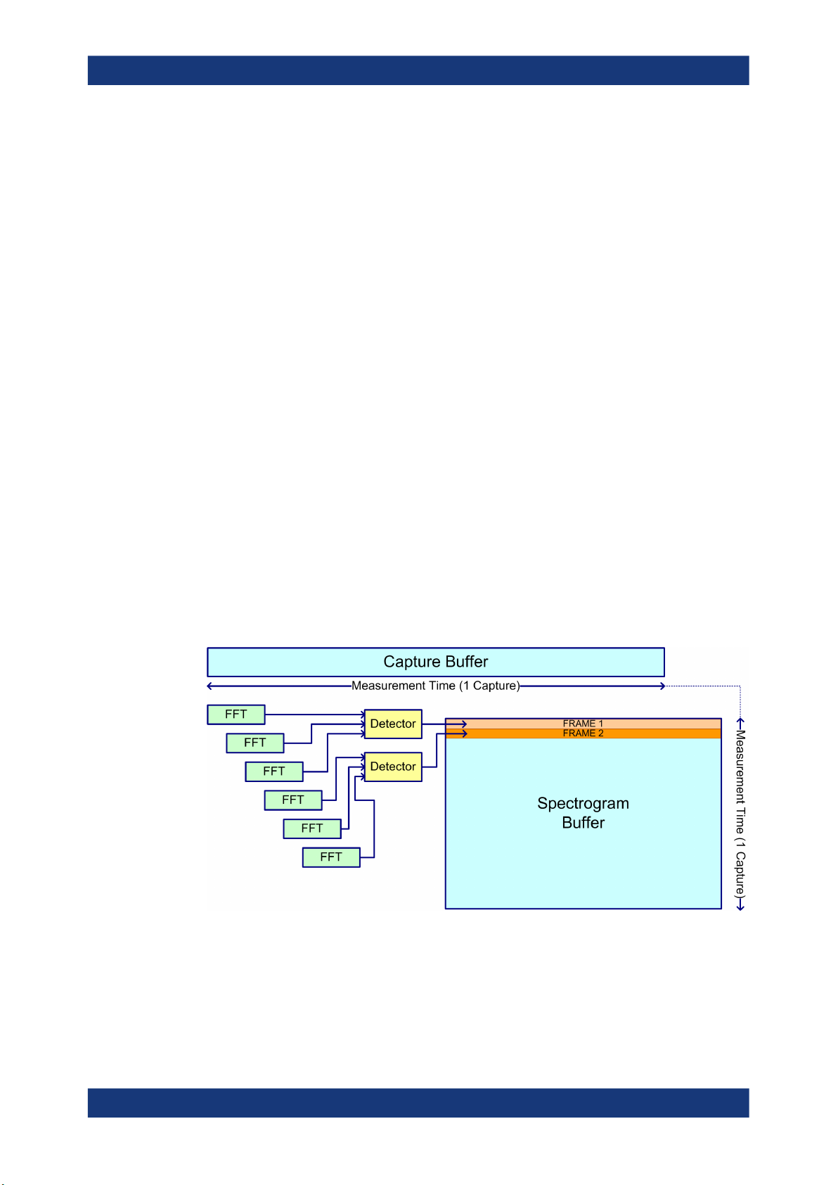
Asynchronous data processing
During a measurement in the R&S FSV3 Transient Analysis application, the data is
captured and stored in the capture buffer until the defined measurement time has
expired. As soon as a minimum amount of data is available, the first FFT calculation is
performed. As soon as the required number of (overlapping) FFT results is available,
the detector function is applied to the data and the first frame is displayed in the Spectrogram (and any other active result displays).
Figure 3-1: Signal processing: calculating one spectrogram frame
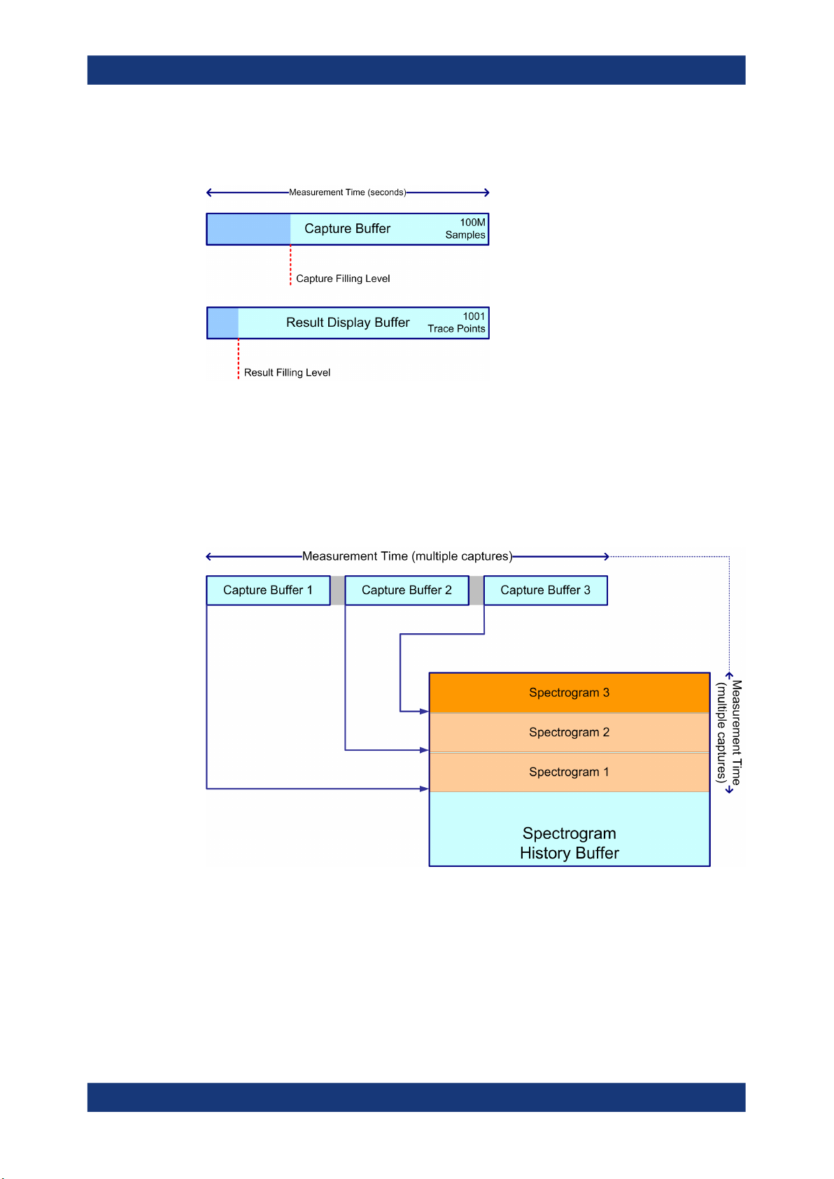
Shortly after the measurement time is over, the final results are displayed and the measurement is complete. Due to this asynchronous processing, initial analysis results are
available very quickly. At the same time, the data is captured over the full bandwidth
16User Manual 1179.3280.02 ─ 06
Page 17
R&S®FSV3-K60
Measurement basics
Signal processing
entirely without gaps. The following figure illustrates how the capture and result display
processes are performed asynchronously.
Figure 3-2: Asynchronous data processing
Multiple spectrograms
However, after each data acquisition, a short delay occurs before the next acquisition
can be carried out. Thus, for measurements for which several spectrograms are
required and the capturing process is repeated several times (defined by the "frame
count"), a short gap in the results between spectrograms can be detected.
Figure 3-3: Signal processing: calculating several spectrograms
Resolution bandwidth
The resolution bandwidth (RBW) has an effect on how the spectrum is measured and
displayed. It determines the frequency resolution of the measured spectrum and is
directly coupled to the selected analysis bandwidth (ABW). The ABW can be the full
measurement bandwidth, the bandwidth of the analysis region, or the length of the
17User Manual 1179.3280.02 ─ 06
Page 18

R&S®FSV3-K60
Measurement basics
Signal models
result range, depending on the evaluation basis of the result display (see Chapter 3.5,
"Basis of evaluation", on page 21). If the ABW is changed, the resolution bandwidth is
automatically adjusted. Which coupling ratios are available depends on the selected
FFT Window.
A small resolution bandwidth has several advantages. The smaller the resolution bandwidth, the better you can observe signals whose frequencies are close together and
the less noise is displayed. However, a small resolution bandwidth also increases the
required measurement time.
The resolution bandwidth parameters can be defined in the bandwidth configuration,
see Chapter 5.6, "Bandwidth settings", on page 101.
Time resolution
The time resolution determines the size of the bins used for each FFT calculation. The
shorter the time span used for each FFT, the shorter the resulting span, and thus the
higher the resolution in the spectrum becomes. The time resolution to be used for
R&S FSV/A can be defined manually or automatically according to the data acquisition
settings.
3.4 Signal models
If the additional firmware options R&S FSV/A-K60H or -K60C are installed, the R&S
FSV3 Transient Analysis application supports different signal models for which similar
parameters are characteristic.
● Frequency hopping................................................................................................. 18
● Frequency chirping..................................................................................................20
● Automatic vs. manual hop/chirp state detection......................................................21
3.4.1 Frequency hopping
Some digital data transmission standards employ a frequency-hopping technique, in
which a carrier signal is rapidly switched among many frequency channels. Discrete
frequencies and continuous modulation are characteristic of this signal model.
18User Manual 1179.3280.02 ─ 06
Page 19

R&S®FSV3-K60
Measurement basics
Signal models
Figure 3-4: Typical spectrogram of a frequency-hopping signal
Analyzing such signals includes the following challenges:
●
Detecting the currently used carrier frequency and a possible offset
●
Determining the duration the signal stays at one frequency and the time it takes to
switch to another
●
Measuring the average power level
●
Demodulating the signal correctly
The R&S FSV3 Transient Analysis application (with the additional R&S FSV/A-K60H
option installed) can automatically detect frequency hops in a measured signal and
determine characteristic hop parameters. Both pulsed and continuous wave hopping
signals can be analyzed.
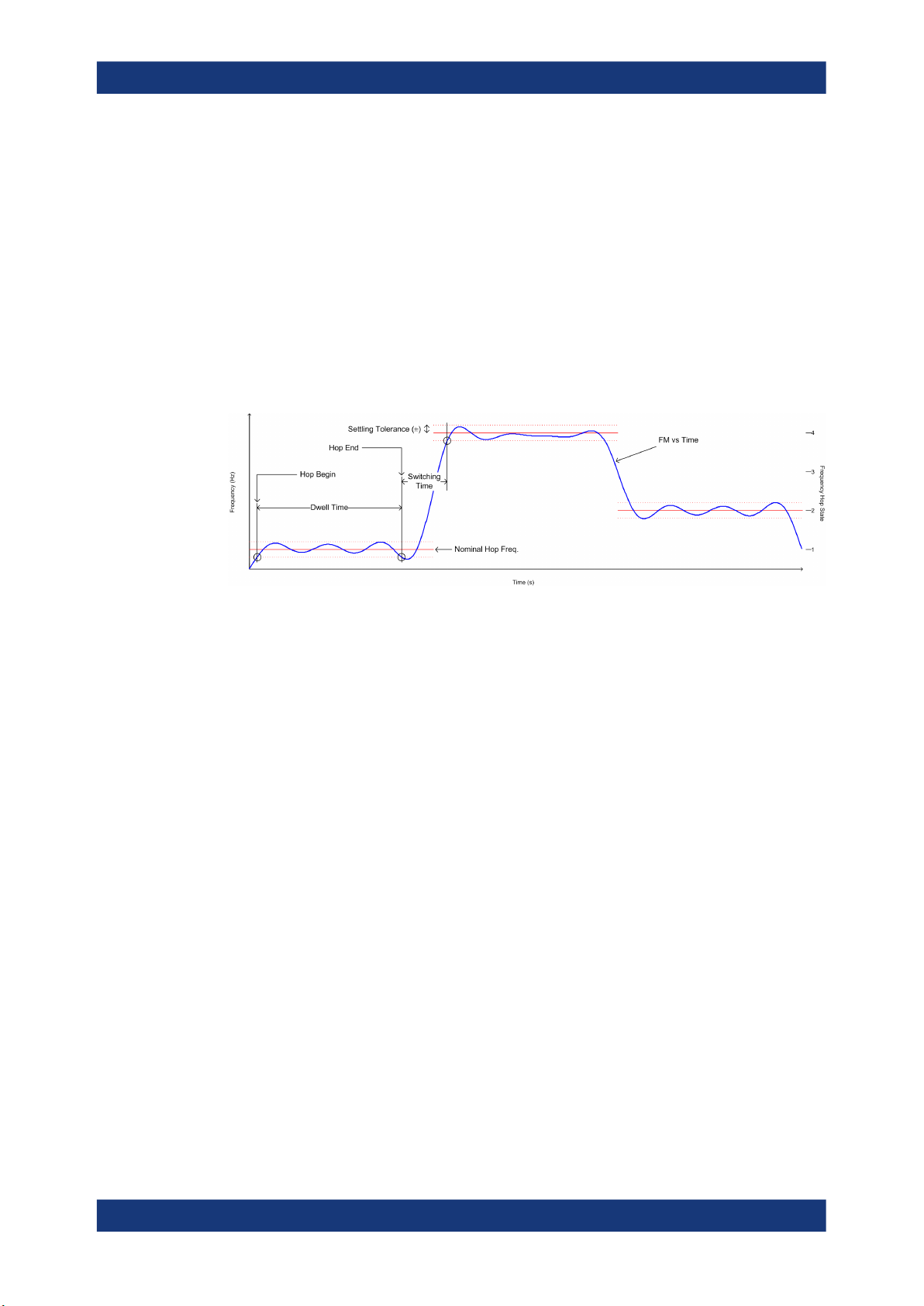
Assuming a frequency-hopping signal model, the frequency bands in which the carrier
can be expected are usually known in advance. Therefore, you can configure conditions that must apply to the measured signal in order to detect a frequency hop and
distinguish it from random spurs or frequency distortions. Such conditions can be a frequency tolerance around a defined nominal value, for instance, or a minimum or maximum dwell time in which the frequency remains steady.
Figure 3-5: Parameters required to detect hops
19User Manual 1179.3280.02 ─ 06
Page 20

R&S®FSV3-K60
Measurement basics
Signal models
Nominal Frequency Values (Hop States)
The (nominal) frequency values the carrier is expected to "hop" to are defined in
advance. Each such level is considered to be a hop state. The hop states are defined
as frequency offsets from the center frequency. A tolerance span can be defined to
compensate for settling effects. As long as the deviation remains within the tolerance
above or below the nominal frequency, the hop state is detected.
The nominal frequency levels are numbered consecutively in the "Hop States" table
(see Chapter 5.2.2, "Signal states", on page 77), starting at 0. The state index of the
corresponding nominal frequency level is assigned to each detected hop in the measured signal results.
Dwell Time Conditions
The dwell time is the time the signal remains in the tolerance area of a nominal hop
frequency, or in other words: the duration of a hop from beginning to end. In a default
measurement, useful dwell times for the current measurement are determined automatically. However, you can define minimum or maximum dwell times, or both, manually, in order to detect only specific hops, for example.
3.4.2 Frequency chirping
Frequency chirping is similar to hopping, however, instead of switching to discrete frequencies, the frequency varies with time at a particular chirp rate. Transient analysis
with the R&S FSV/A application (and the additional R&S FSV/A-K60C option) is restricted to the commonly used linear FM chirp signals. In this case, the nominal chirp
switches to discrete values, referred to as the chirp states.
Figure 3-6: Typical spectrogram of a chirped signal
20User Manual 1179.3280.02 ─ 06
Page 21

R&S®FSV3-K60
Measurement basics
Basis of evaluation
The R&S FSV3 Transient Analysis application can automatically detect chirps in a
measured signal and determine characteristic chirp parameters. Both pulsed and continuous wave chirp signals can be analyzed.
Obviously, if you consider the chirps rather than the individual frequencies, the measured data from chirped signals is very similar to hopped signals, and thus the analysis
tasks and the characteristic parameters are very similar, as well.
Figure 3-7: Parameters required to detect chirps
In the R&S FSV3 Transient Analysis application, for a chirp signal, the derivation of the
captured signal data is calculated before further analysis. From there, processing is
identical for both signal models.
3.4.3 Automatic vs. manual hop/chirp state detection
By default, the R&S FSV3 Transient Analysis application automatically detects the
existing hop/chirp states in a pre-measurement. For an initial overview of the signal at
hand this detection is usually sufficient. For more accurate results, particularly if the
input signal is known in advance, the nominal frequency or chirp values can be defined
manually.
3.5 Basis of evaluation
Depending on the measurement task, not all of the measured data in the capture buffer
may be of interest. In some cases it may be useful to restrict analysis to a specific
user-definable region, or to a selected individual chirp or hop. This makes analysis
more efficient and the display clearer.
Automatic detection of hops or chirps, for example, is always based on a restricted
analysis region. Numeric results for characteristic parameters, as well as statistical
results, are also calculated on this restricted basis.
For graphical displays, selecting an individual hop or chirp allows you to analyze or
compare characteristic values in detail.
Which evaluation basis is available for which result display is indicated in Table 4-1.
21User Manual 1179.3280.02 ─ 06
Page 22

R&S®FSV3-K60
Measurement basics
Analysis region
Detected hops/chirps are indicated by green bars along the x-axis in graphical result
displays. The selected hop/chirp (see "Select Hop / Select Chirp" on page 120) is indicated by a blue bar. The hop/chirp index as displayed in the result tables is indicated at
the bottom of each bar.
Figure 3-8: Example of detected hops with hop index in graphical result display and result table
3.6 Analysis region
The analysis region determines which of the captured data is analyzed and displayed
on the screen. By default, the entire capture buffer data is defined as the analysis
region. However, you can select a specific frequency and time region which is of interest for analysis. The results can then be restricted to this region (see Chapter 6.3,
"Evaluation basis", on page 120).
Note, however, that only one analysis region can be defined. All result displays that are
restricted to the analysis region thus have the same data basis.
22User Manual 1179.3280.02 ─ 06
Page 23

R&S®FSV3-K60
Measurement basics
Analysis region
Numeric results (displayed in the result or statistics tables) are always calculated
based on the analysis region.
For graphical result displays based on the analysis region, the x-axis range corresponds to the analysis region length (see "Time Gate Length" on page 100).
The analysis region is indicated by a colored frame in the Full Spectrogram display,
and by vertical blue lines in result displays based on the full capture buffer.
The colors used to indicate the analysis range in spectrograms are configurable, see
"Modifying Analysis Region and Sweep Separator Colors" on page 128.
Defining the analysis region
There are different methods of defining the analysis region:
●
absolute definition: by defining an absolute frequency span and an absolute time
gate
The frequency span is defined by an offset from the center frequency and an analysis bandwidth.
The time gate is defined by a starting point after measurement begin and the gate
length.
●
Relative definition: by linking the analysis region to the full capture buffer and defining a percentage of the full bandwidth and measurement time
The specified frequency offset or time gate start are also considered for relative
values.
●
Graphically: The analysis region is indicated by a dotted frame in the Spectrogram
display and by vertical lines in the full spectrum display. Its size and position can be
moved by tapping and dragging the frame on the touchscreen.
Furthermore, the data zoom and shift functions allow you to change the size and
position of the analysis region from any graphical result display (see Chapter 3.7,
"Zooming and shifting results", on page 25).
The absolute and relative methods can be combined, for example by defining an absolute frequency span and a relative time gate.
23User Manual 1179.3280.02 ─ 06
Page 24

R&S®FSV3-K60
Measurement basics
Analysis region
Figure 3-9: Visualization of absolute analysis region parameters
Processing data in the analysis region - data zoom
In result displays restricted to the analysis region, only the data measured for the
specified frequency range and within the defined time gate is considered. Furthermore,
the analysis region data is taken only from the latest data acquisition, that is, only data
that is still in the capture buffer is analyzed.
Restricting the results to an analysis region has the same effect as a data zoom: the
results are recalculated for a restricted data base. The data in the capture buffer is filtered by the defined time gate; the measured data within that time span then passes a
bandpass filter, so only the frequency range of interest is analyzed. Depending on the
selected result display, the data is then demodulated, if necessary, and distributed
among the trace points using a detector. The time span displayed per division of the
diagram is much smaller compared to the initial full data analysis. Thus, the results of
the analysis range become more precise.
24User Manual 1179.3280.02 ─ 06
Page 25

R&S®FSV3-K60
Measurement basics
Zooming and shifting results
Figure 3-10: Data zoom - full result vs. analysis region result
3.7 Zooming and shifting results
As described above (Processing data in the analysis region - data zoom), restricting
the results to an analysis region has the same effect as a data zoom: the results are
recalculated for a restricted data base.
This is exactly what the "Data Zoom" ( ) function in the toolbar does: it changes the
size of the analysis region and re-evaluates the new data base. Thus, if the analysis
region is reduced, less data is displayed in the same area of the screen, thus enlarging
the display of the selected data. If the analysis region is enlarged, more data is displayed.
The "Data Shift" ( ) function, on the other hand, does not change the size of the
analysis region, but the position. Thus you can scroll through the signal and analyze
several hops/chirps after another, for example.
The effects of a data zoom or shift are reflected in the Analysis Region settings of the
"Data Acquisition" dialog box.
Similarly, when the data zoom and shift functions are applied to a hop/chirp-based
result display, the size or position of the result range are changed (see Chapter 6.2.1,
"Result range", on page 112).
This means that ALL result displays based on the analysis region or hop/chirp result
range are re-evaluated after a data zoom or shift function is applied in any window.
This includes result tables, which may take some time to re-calculate. Close the result
tables during a data shift/zoom to improve the screen update speed.
25User Manual 1179.3280.02 ─ 06
Page 26

R&S®FSV3-K60
3.8 Measurement range
Measurement basics
Measurement range
Use the data zoom or shift functions in the full spectrum or spectrogram displays and
analyze the data sequentially or hop-by-hop / chirp-by-chirp in the other result displays!
In order to calculate frequency, phase or power results in frequency hopping or chirped
signals more accurately, it may be useful not to take the entire dwell time of the hop (or
length of the chirp) into consideration, but only a certain range within the dwell time/
length. Thus, it is possible to eliminate settling effects, for instance. For other measurements, the settling time may be of particular interest.
For such cases, a measurement range can be defined for frequency, phase and power
results, in relation to specific hop or chirp characteristics.
Figure 3-11: Dwell time parameters for hopped signals
Similarly, for chirped signals, a measurement range can be defined for the corresponding parameters.
26User Manual 1179.3280.02 ─ 06
Page 27

R&S®FSV3-K60
Measurement basics
Measurement range
Figure 3-12: Measurement range parameters for chirped signals
Each range is defined by a reference point, an offset, and the range length. The reference point can be either the center or either edge of the hop/chirp, or a point defined
by an offset to one of these characteristic points. The range is then centered around
this reference point.
Example:
In Figure 3-11, the indicated measurement range could be defined by the following
parameters, for example:
●
"Reference": Hop End
●
"Offset": -x
●
"Alignment": right
●
"Length": L
For frequency/phase deviation and power measurements, the measurement range can
also be aligned to the end of the FM or PM settling time.
27User Manual 1179.3280.02 ─ 06
Page 28

R&S®FSV3-K60
3.9 Trace evaluation
Measurement basics
Trace evaluation
Measurement range vs result range
While the measurement range defines which part of the hop/chirp is used for individual
calculations, the result range determines which part is displayed on the screen in the
form of AM, FM or PM vs. time traces (see also Chapter 6.2.1, "Result range",
on page 112).
Traces in graphical result displays based on the defined result range (see Chap-
ter 6.2.1, "Result range", on page 112) can be configured, for example to perform stat-
istical evaluations over the selected hop/chirp or all hops/chirps.
You can configure up to 6 individual traces for the following result displays (see Chap-
ter 4.3, "Evaluation methods for transient analysis", on page 62):
●
RF Power Time Domain
●
FM Time Domain
●
Frequency Deviation Time Domain
●
PM Time Domain
●
PM Time Domain (Wrapped)
●
Chirp Rate Time Domain
Find out more about trace evaluation:
● Mapping samples to measurement points with the trace detector..........................28
● Analyzing several traces - trace mode....................................................................30
● Trace statistics........................................................................................................ 31
3.9.1 Mapping samples to measurement points with the trace detector
A trace displays the values measured at the measurement points. The number of samples taken during a measurement is much larger than the number of measurement
points that are displayed in the measurement trace.
Obviously, a data reduction must be performed to determine which of the samples are
displayed for each measurement point. This is the trace detector's task.
The trace detector can analyze the measured data using various methods:
The detector activated for the specific trace is indicated in the corresponding trace
information by an abbreviation.
28User Manual 1179.3280.02 ─ 06
Page 29

R&S®FSV3-K60
Measurement basics
Trace evaluation
Table 3-1: Detector types
Detector Abbrev. Description
Positive Peak Pk Determines the largest of all positive peak values of the levels measured at the
individual frequencies which are displayed in one sample point
Negative Peak Mi Determines the smallest of all negative peak values of the levels measured at
the individual frequencies which are displayed in one sample point
Auto Peak Ap Combines the peak detectors; determines the maximum and the minimum
value of the levels measured at the individual frequencies which are displayed
in one sample point
RMS Rm Calculates the root mean square of all samples contained in a measurement
point.
The RMS detector supplies the power of the signal irrespective of the wave-
form (CW carrier, modulated carrier, white noise or impulsive signal). Correction factors as needed for other detectors to measure the power of the different
signal classes are not required.
Average Av Calculates the linear average of all samples contained in a measurement
point.
To this effect, R&S FSV/A uses the linear voltage after envelope detection. The
sampled linear values are summed up and the sum is divided by the number of
samples (= linear average value). For logarithmic display the logarithm is
formed from the average value. For linear display the average value is displayed. Each measurement point thus corresponds to the average of the measured values summed up in the measurement point.
The average detector supplies the average value of the signal irrespective of
the waveform (CW carrier, modulated carrier, white noise or impulsive signal).
Sample Sa Selects the last measured value of the levels measured at the individual fre-
quencies which are displayed in one sample point; all other measured values
for the frequency range are ignored
The result obtained from the selected detector for a measurement point is displayed as
the value at this x-axis point in the trace.
Meas. point n+1
SAMPLE
MAX PEAK
AUTO PEAK
MIN PEAK
AVG
RMS
Video
Signal
Measurement point n
video
video
signal
signal
s1 s2 s3 s4 s5 s6 s8 s1
s1 s2 s3 s4 s5 s6 s8 s1
The trace detector for the individual traces can be selected manually by the user or set
automatically by the R&S FSV/A.
29User Manual 1179.3280.02 ─ 06
Page 30

R&S®FSV3-K60
Measurement basics
Trace evaluation
The detectors of the R&S FSV/A are implemented as pure digital devices. All detectors
work in parallel in the background, which means that the measurement speed is independent of the detector combination used for different traces.
Auto detector
If the R&S FSV/A is set to define the appropriate detector automatically, the detector is
set depending on the selected trace mode:
Trace mode Detector
Clear Write Auto Peak
Max Hold Positive Peak
Min Hold Negative Peak
Average Sample Peak
View –
Blank –
3.9.2 Analyzing several traces - trace mode
If several measurements are performed one after the other, or continuous measurements are performed, the trace mode determines how the data for subsequent traces
is processed. After each measurement, the trace mode determines whether:
●
The data is frozen (View)
●
The data is hidden (Blank)
●
The data is replaced by new values (Clear Write)
●
The data is replaced selectively (Max Hold, Min Hold, Average)
Each time the trace mode is changed, the selected trace memory is cleared.
The trace mode also determines the detector type if the detector is set automatically,
see Chapter 3.9.1, "Mapping samples to measurement points with the trace detector",
on page 28.
The R&S FSV/A offers the following trace modes:
Table 3-2: Overview of available trace modes
Trace Mode Description
Blank Hides the selected trace.
Clear Write Overwrite mode: the trace is overwritten by each measurement. This is the default set-
ting.
All available detectors can be selected.
30User Manual 1179.3280.02 ─ 06
Page 31

R&S®FSV3-K60
Measurement basics
Trace evaluation
Trace Mode Description
Max Hold The maximum value is determined over several measurements and displayed. The
R&S FSV/A saves the measurement result in the trace memory only if the new value
is greater than the previous one.
This mode is especially useful with modulated or pulsed signals. The signal spectrum
is filled up upon each measurement until all signal components are detected in a kind
of envelope.
Min Hold The minimum value is determined from several measurements and displayed. The
R&S FSV/A saves the measurement result in the trace memory only if the new value
is lower than the previous one.
This mode is useful e.g. for making an unmodulated carrier in a composite signal visible. Noise, interference signals or modulated signals are suppressed, whereas a CW
signal is recognized by its constant level.
Average The average is formed over several measurements and displayed. The Sweep/Aver-
age Count determines the number of averaging procedures.
(See also Chapter 3.9.3, "Trace statistics", on page 31.)
View The current contents of the trace memory are frozen and displayed.
If a trace is frozen ("View" mode), the instrument settings, apart from level range and
reference level (see below), can be changed without impact on the displayed trace.
The fact that the displayed trace no longer matches the current instrument setting is
indicated by the icon on the tab label.
If the level range or reference level is changed, the R&S FSV/A automatically adapts
the trace data to the changed display range. This allows an amplitude zoom to be
made after the measurement in order to show details of the trace.
3.9.3 Trace statistics
Each trace represents an analysis of the data measured in one result range. As described in Chapter 3.9.2, "Analyzing several traces - trace mode", on page 30, statistical
evaluations can be performed over several traces, that is, result ranges. Which ranges
and how many are evaluated depends on the configuration settings.
Selected hop/chirp vs all hops/chirps
The Sweep/Average Count determines how many measurements are evaluated.
For each measurement, in turn, either the selected hop/chirp only (that is: one result
range), or all detected hops/chirps (that is: possibly several result ranges) can be included in the statistical evaluation.
Thus, the overall number of averaging steps depends on the Sweep/Average Count
and the statistical evaluation mode.
31User Manual 1179.3280.02 ─ 06
Page 32

R&S®FSV3-K60
Measurement basics
Working with spectrograms
Figure 3-13: Trace statistics - number of averaging steps
3.10 Working with spectrograms
In addition to the standard "level versus frequency" or "level versus time" traces, the
R&S FSV/A also provides a spectrogram display of the measured data.
A spectrogram shows how the spectral density of a signal varies over time. The x-axis
shows the frequency, the y-axis shows the time. A third dimension, the power level, is
indicated by different colors. Thus you can see how the strength of the signal varies
over time for different frequencies.
32User Manual 1179.3280.02 ─ 06
Page 33

R&S®FSV3-K60
Measurement basics
Working with spectrograms
Example:
In this example, you see the spectrogram for the calibration signal of the R&S FSV/A,
compared to the standard spectrum display. Since the signal does not change over
time, the color of the frequency levels does not change over time, i.e. vertically. The
legend above the spectrogram display describes the power levels the colors represent.
Result display
The spectrogram result can consist of the following elements:
1
6
2
5
3
4
88
7
Figure 3-14: Screen layout of the spectrogram result display
1 = Spectrum result display
2 = Spectrogram result display
3 = Marker list
4 = Marker
33User Manual 1179.3280.02 ─ 06
Page 34

R&S®FSV3-K60
Measurement basics
Working with spectrograms
5 = Delta marker
6 = Color map
7 = Timestamp / frame number
8 = Current frame indicator
For more information about spectrogram configuration, see Chapter 6.6, "Spectrogram
settings", on page 126.
Remote commands:
Activating and configuring spectrograms:
Chapter 10.6.10, "Configuring spectrograms", on page 324
Storing results:
MMEMory:STORe<n>:SPECtrogram on page 422
● Time frames............................................................................................................ 34
● Markers in the spectrogram.................................................................................... 35
● Color maps..............................................................................................................35
3.10.1 Time frames
The time information in the spectrogram is displayed vertically, along the y-axis. Each
line (or trace) of the y-axis represents one or more captured measurement and is
called a time frame or simply "frame". As with standard spectrum traces, several measured values are combined in one measurement point using the selected detector.
Frames are sorted in chronological order, beginning with the most recently recorded
frame at the top of the diagram (frame number 0). With the next measurement, the previous frame is moved further down in the diagram, until the maximum number of captured frames is reached. The display is updated continuously during the measurement,
and the measured trace data is stored. Spectrogram displays are continued even after
single measurements unless they are cleared manually.
The frames for each individual sweep are separated by colored lines.
The scaling of the time axis (y-axis) is not configurable. However, you can enlarge the
spectrogram display by maximizing the window using the "Split/Maximize" key.
Alternatively, use a spectrogram based on the analysis region and decrease the size of
the region to zoom into the data of interest. (See also Chapter 3.7, "Zooming and shift-
ing results", on page 25.)
Tracking absolute time - timestamps
Alternatively to the frame count, the absolute time (that is: a timestamp) at which a
frame was captured can be displayed. While the measurement is running, the timestamp shows the system time. In single measurement mode or if the measurement is
34User Manual 1179.3280.02 ─ 06
Page 35

R&S®FSV3-K60
3.10.2 Markers in the spectrogram
Measurement basics
Working with spectrograms
stopped, the timestamp shows the time and date at the end of the measurement.Thus,
the individual frames can be identified by their timestamp or their frame count.
When active, the timestamp replaces the display of the frame number in the diagram
footer (see Figure 3-14).
Displaying individual frames
The spectrogram diagram contains all stored frames since it was last cleared. Arrows
on the left and right border of the spectrogram indicate the currently selected frame.
The spectrum diagram always displays the spectrum for the currently selected frame.
The current frame number is indicated in the diagram footer, or alternatively a timestamp, if activated. The current frame, displayed at the top of the diagram, is frame
number 0. Older frames further down in the diagram are indicated by a negative index,
e.g."-10". You can display the spectrum diagram of a previous frame by changing the
current frame number.
Markers and delta markers are shaped like diamonds in the spectrogram. They are
only displayed in the spectrogram if the marker position is inside the visible area of the
spectrogram. If more than two markers are active, the marker values are displayed in a
separate marker table.
In the spectrum result display, the markers and their frequency and level values (1) are
displayed as usual. Additionally, the frame number is displayed to indicate the position
of the marker in time (2).
In the spectrogram result display, you can activate up to 16 markers or delta markers
at the same time. Each marker can be assigned to a different frame. Therefore, in
addition to the frequency you also define the frame number when activating a new
marker. If no frame number is specified, the marker is positioned on the currently
selected frame. All markers are visible that are positioned on a visible frame. Special
search functions are provided for spectrogram markers.
In the spectrum result display, only the markers positioned on the currently selected
frame are visible. In "Continuous Sweep" mode, this means that only markers positioned on frame 0 are visible. To view markers that are positioned on a frame other
than frame 0 in the spectrum result display, you must stop the measurement and select
the corresponding frame.
3.10.3 Color maps
Spectrograms assign power levels to different colors to visualize them. The legend
above the spectrogram display describes the power levels the colors represent.
35User Manual 1179.3280.02 ─ 06
Page 36

R&S®FSV3-K60
Measurement basics
Working with spectrograms
The color display is highly configurable to adapt the spectrograms to your needs. You
can define:
●
Which colors to use (Color scheme)
●
Which value range to apply the color scheme to
●
How the colors are distributed within the value range, i.e where the focus of the visualization lies (shape of the color curve)
The individual colors are assigned to the power levels automatically by the
R&S FSV/A.
The Color Scheme
For each color scheme, you can select the suitable color used to display the analysis
region frame and sweep separator lines, see "Modifying Analysis Region and Sweep
Separator Colors" on page 128.
●
Hot
Uses a color range from blue to red. Blue colors indicate low levels, red colors indicate high ones.
●
Cold
Uses a color range from red to blue. Red colors indicate low levels, blue colors
indicate high ones.
The "Cold" color scheme is the inverse "Hot" color scheme.
●
Radar
Uses a color range from black over green to light turquoise with shades of green in
between. Dark colors indicate low levels, light colors indicate high ones.
●
Grayscale
Shows the results in shades of gray. Dark gray indicates low levels, light gray indicates high ones.
The value range of the color map
If the measured values only cover a small area in the spectrogram, you can optimize
the displayed value range. Then it becomes easier to distinguish between values that
are close together. Display only parts of interest.
The shape and focus of the color curve
The color-mapping function assigns a specified color to a specified power level in the
spectrogram display. By default, colors on the color map are distributed evenly. How-
36User Manual 1179.3280.02 ─ 06
Page 37

R&S®FSV3-K60
Measurement basics
Working with spectrograms
ever, to visualize a certain area of the value range in greater detail than the rest, you
can set the focus of the color mapping to that area. Changing the focus is performed
by changing the shape of the color curve.
The color curve is a tool to shift the focus of the color distribution on the color map. By
default, the color curve is linear. If you shift the curve to the left or right, the distribution
becomes non-linear. The slope of the color curve increases or decreases. One end of
the color palette then covers a large range of results, while the other end distributes
several colors over a relatively small result range.
You can use this feature to put the focus on a particular region in the diagram and to be
able to detect small variations of the signal.
37User Manual 1179.3280.02 ─ 06
Page 38

R&S®FSV3-K60
Measurement basics
Working with spectrograms
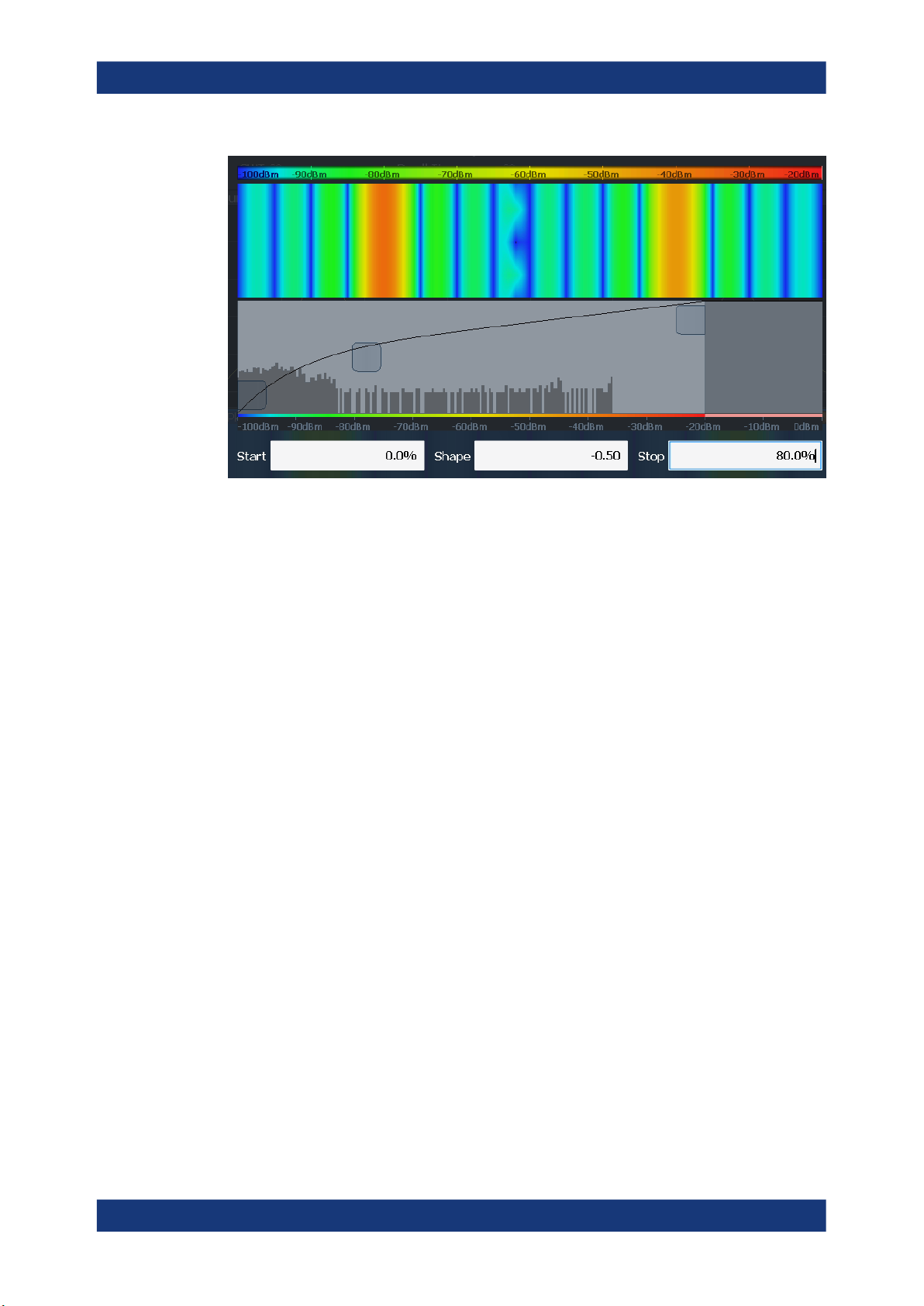
Example:
In the color map based on the linear color curve, the range from -100 dBm to -60 dBm
is covered by blue and a few shades of green only. The range from -60 dBm to
-20 dBm is covered by red, yellow and a few shades of green.
Figure 3-15: Spectrogram with (default) linear color curve shape = 0
The sample spectrogram is dominated by blue and green colors. After shifting the color
curve to the left (negative value), more colors cover the range from -100 dBm to
-60 dBm (blue, green and yellow). This range occurs more often in the example. The
range from -60 dBm to -20 dBm, on the other hand, is dominated by various shades of
red only.
38User Manual 1179.3280.02 ─ 06
Page 39
R&S®FSV3-K60
Measurement basics
Working with spectrograms
Figure 3-16: Spectrogram with non-linear color curve (shape = -0.5)
39User Manual 1179.3280.02 ─ 06
Page 40

R&S®FSV3-K60
4 Measurement results
Measurement results
The data that was measured by the R&S FSV/A can be evaluated using various different methods.
Basis of evaluation
For some displays you can define whether the results are calculated for:
●
the entire capture buffer
●
the selected analysis region
●
a selected individual chirp or hop (for options R&S FSV/A-K60C/-K60H)
Figure 4-1: Example for different data sources for the same result display (FM Time Domain)
The data source for each result display is selected in the [MEAS] menu. It is indicated
in the description of the individual result displays.
The analysis region is indicated by a colored frame in the Full Spectrogram display,
and by vertical blue lines in result displays based on the full capture buffer. For details
on the analysis region see Chapter 3.6, "Analysis region", on page 22.
For hop/chirp-based result displays, the current hop/chirp index as displayed in the
result tables is indicated at the bottom of the hop/chirp bar.
Measurement range vs result range
The measurement range defines which part of a hop/chirp is used for calculation (for
example for frequency estimation), whereas the result range determines which data is
displayed on the screen in the form of AM, FM or PM vs. time traces.
Exporting Table Results to an ASCII File
Measurement result tables can be exported to an ASCII file for further evaluation in
other (external) applications.
For step-by-step instructions on how to export a table, see Chapter 7.2, "How to export
table data", on page 155.
● Hop parameters...................................................................................................... 41
● Chirp parameters.................................................................................................... 51
● Evaluation methods for transient analysis...............................................................62
40User Manual 1179.3280.02 ─ 06
Page 41
R&S®FSV3-K60
4.1 Hop parameters
Measurement results
Hop parameters
If the R&S FSV/A-K60H option is installed, various hop parameters can be determined
during transient analysis.
The hop parameters to be measured are based primarily on the IEEE 181 Standard
181-2003. For detailed descriptions refer to the standard documentation ("IEEE Standard on Transitions, hops, and Related Waveforms", from the IEEE Instrumentation
and Measurement (I&M) Society, 7 July 2003).
The following graphic illustrates the main hop parameters and characteristic values.
(For a definition of the values used to determine the measured hop parameters see
Chapter 3.4.1, "Frequency hopping", on page 18.)
Figure 4-2: Definition of the main hop parameters and characteristic values
In order to obtain these results, select the corresponding parameter in the result configuration (see Chapter 6.2.2, "Table configuration", on page 113) or apply the required
SCPI parameter to the remote command (see Chapter 10.6.5.2, "Hop results",
on page 257 and Chapter 10.7.1, "Retrieving information on detected hops",
on page 356).
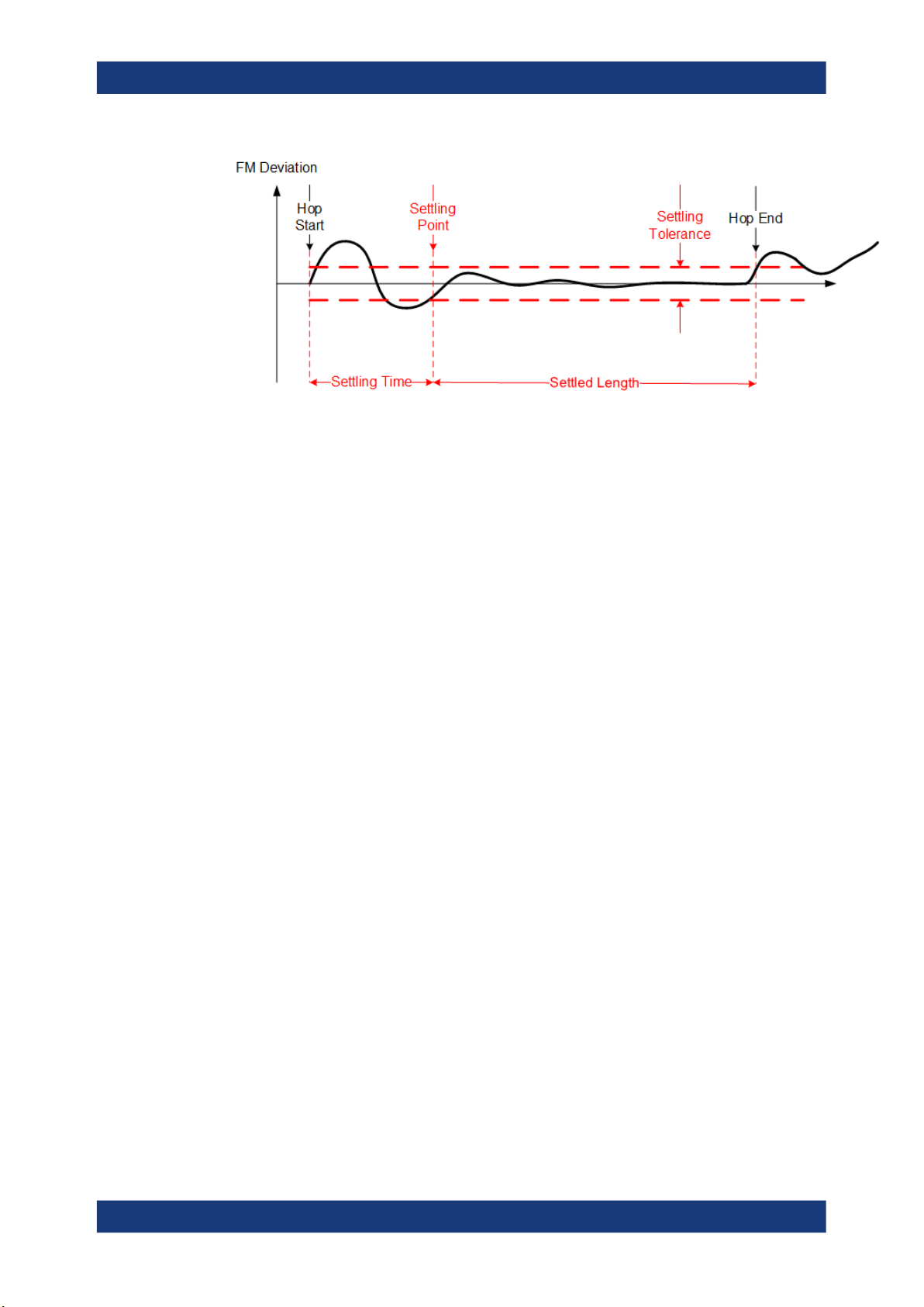
Settling Parameters
Settling refers to the time it takes the FM or PM signal to remain within a specified tolerance around the nominal frequency.
Settling parameters are calculated from the FM or PM deviation considering the given
FM or PM settling tolerance.
41User Manual 1179.3280.02 ─ 06
Page 42
R&S®FSV3-K60
Measurement results
Hop parameters
Figure 4-3: Settling parameters for hopped signals
Hop ID and Hop number
Each individual hop can be identified by a timestamp which corresponds to the absolute time the beginning of the hop was detected. In addition, each hop is provided with
a consecutive number, which starts at 1 for each new measurement. This is useful to
distinguish hops in a measurement quickly.
Remote command:
[SENSe:]HOP:ID? on page 371
[SENSe:]HOP:NUMBer? on page 377
State parameters...........................................................................................................43
└ State Index......................................................................................................43
Timing parameters........................................................................................................ 43
└ Hop Begin....................................................................................................... 43
└ Dwell Time...................................................................................................... 43
└ Switching Time................................................................................................44
Frequency parameters..................................................................................................44
└ State Frequency (Nominal).............................................................................44
└ Average Frequency.........................................................................................44
└ Hop State Deviation........................................................................................44
└ Relative Frequency (Hop-to-Hop)...................................................................45
└ Frequency Deviation (Peak)........................................................................... 45
└ Frequency Deviation (RMS)............................................................................45
└ Frequency Deviation (Average)...................................................................... 46
Phase parameters.........................................................................................................46
└ Phase Deviation (Peak).................................................................................. 47
└ Phase Deviation (RMS).................................................................................. 48
└ Phase Deviation (Average).............................................................................48
Power parameters.........................................................................................................48
└ Minimum Power.............................................................................................. 48
└ Maximum Power............................................................................................. 49
└ Average Power............................................................................................... 49
└ Power Ripple...................................................................................................49
42User Manual 1179.3280.02 ─ 06
Page 43

R&S®FSV3-K60
Measurement results
Hop parameters
FM settling parameters................................................................................................. 49
└ FM settling point..............................................................................................49
└ FM settling time...............................................................................................50
└ FM settled length............................................................................................ 50
PM settling parameters................................................................................................. 50
└ PM settling point............................................................................................. 50
└ PM settling time.............................................................................................. 51
└ PM settled length............................................................................................ 51
State parameters
Hop state parameters
Remote command:
CALCulate<n>:HOPDetection:TABLe:STATe:ALL[:STATe] on page 264
State Index ← State parameters
The nominal frequency levels are numbered consecutively in the "Hop States" table
(see Chapter 5.2.2, "Signal states", on page 77), starting at 0. The state of a detected
hop is defined as the index of the corresponding nominal frequency.
Remote command:
Display:
CALCulate<n>:HOPDetection:TABLe:STATe:INDex on page 265
Results:
CALCulate<n>:HOPDetection:TABLe:RESults? on page 358
[SENSe:]HOP:STATe[:INDex]? on page 380
Timing parameters
Hop timing parameters
Remote command:
CALCulate<n>:HOPDetection:TABLe:TIMing:ALL[:STATe] on page 266
Hop Begin ← Timing parameters
The relative time (in ms) from the capture start at which the signal first enters the tolerance area of a nominal hop (within the analysis region). The tolerance area is defined
by the settling tolerance above and below the defined nominal hop frequencies.
Remote command:
Display:
CALCulate<n>:HOPDetection:TABLe:TIMing:BEGin on page 266
Results:
CALCulate<n>:HOPDetection:TABLe:RESults? on page 358
[SENSe:]HOP:TIMing:BEGin? on page 382
Dwell Time ← Timing parameters
The duration of a hop from begin to end, that is, the time the signal remains in the tolerance area of a nominal hop frequency.
Remote command:
Display:
CALCulate<n>:HOPDetection:TABLe:TIMing:DWELl on page 266
Results:
43User Manual 1179.3280.02 ─ 06
Page 44

R&S®FSV3-K60
Measurement results
Hop parameters
CALCulate<n>:HOPDetection:TABLe:RESults? on page 358
[SENSe:]HOP:TIMing:DWELl? on page 383
Switching Time ← Timing parameters
The time the signal requires to "hop" from one level to the next. It is defined as the time
between a hop end and the following hop begin. The first switching time result can only
be determined after the first hop has been detected.
Remote command:
Display:
CALCulate<n>:HOPDetection:TABLe:TIMing:SWITching on page 266
Results:
CALCulate<n>:HOPDetection:TABLe:RESults? on page 358
[SENSe:]HOP:TIMing:SWITching? on page 384
Frequency parameters
Hop frequency parameters
Remote command:
CALCulate<n>:HOPDetection:TABLe:STATe:ALL[:STATe] on page 264
State Frequency (Nominal) ← Frequency parameters
Nominal frequency of the hop state as defined in "Hop States" table.
Remote command:
Display:
CALCulate<n>:HOPDetection:TABLe:STATe:STAFrequency on page 265
Results:
CALCulate<n>:HOPDetection:TABLe:RESults? on page 358
[SENSe:]HOP:STATe:STAFrequency? on page 381
Average Frequency ← Frequency parameters
Average frequency measured within the frequency measurement range of the hop (see
Chapter 5.7, "Hop / chirp measurement settings", on page 103).
Remote command:
Display:
CALCulate<n>:HOPDetection:TABLe:FREQuency:AVGFm on page 261
Results:
CALCulate<n>:HOPDetection:TABLe:RESults? on page 358
[SENSe:]HOP:FREQuency:FREQuency? on page 368
Hop State Deviation ← Frequency parameters
Deviation of the hop frequency from the nominal hop state frequency
Where
●
: Average hop frequency estimate obtained from the frequency meas range of a
hop
●
f
: Nominal hop frequency corresponding to a detected or predefined hop state
nom
44User Manual 1179.3280.02 ─ 06
Page 45

R&S®FSV3-K60
Measurement results
Hop parameters
Remote command:
Display:
CALCulate<n>:HOPDetection:TABLe:FREQuency:FMERror on page 261
Results:
CALCulate<n>:HOPDetection:TABLe:RESults? on page 358
[SENSe:]HOP:FREQuency:FMERror? on page 367
Relative Frequency (Hop-to-Hop) ← Frequency parameters
Relative difference in frequency between two hops.
Remote command:
Display:
CALCulate<n>:HOPDetection:TABLe:FREQuency:RELFrequency on page 261
Results:
CALCulate<n>:HOPDetection:TABLe:RESults? on page 358
[SENSe:]HOP:FREQuency:RELFrequency? on page 370
Frequency Deviation (Peak) ← Frequency parameters
Maximum of Frequency Deviation vs Time trace
All hop frequency deviation table values are calculated from the time domain result:
for hop start ≤ k ≤ hop start + dwell time
where:
f
(k): instantaneous frequency of the measured signal
meas
f
(k): ideal frequency trajectory obtained from weighted linear regression of the
ideal
instantaneous signal phase
φ
(k) within the frequency measurement range (see
meas
Chapter 5.7, "Hop / chirp measurement settings", on page 103)
The peak deviation is thus defined as:
for k∈ {frequency meas range}
Remote command:
Display:
CALCulate<n>:HOPDetection:TABLe:FREQuency:MAXFm on page 261
Results:
CALCulate<n>:HOPDetection:TABLe:RESults? on page 358
[SENSe:]HOP:FREQuency:MAXFm? on page 369
Frequency Deviation (RMS) ← Frequency parameters
RMS of Frequency Deviation vs Time trace
for k∈ {frequency meas range}
(fdev is defined in "Frequency Deviation (Peak)" on page 45)
45User Manual 1179.3280.02 ─ 06
Page 46

R&S®FSV3-K60
Measurement results
Hop parameters
Remote command:
Display:
CALCulate<n>:HOPDetection:TABLe:FREQuency:RMSFm on page 261
Results:
CALCulate<n>:HOPDetection:TABLe:RESults? on page 358
[SENSe:]HOP:FREQuency:RMSFm? on page 371
Frequency Deviation (Average) ← Frequency parameters
Average of Frequency Deviation vs Time trace
for k∈ {frequency meas range}
(fdev is defined in "Frequency Deviation (Peak)" on page 45)
Remote command:
Display:
CALCulate<n>:HOPDetection:TABLe:FREQuency:AVGFm on page 261
Results:
CALCulate<n>:HOPDetection:TABLe:RESults? on page 358
[SENSe:]HOP:FREQuency:AVGFm? on page 364
Phase parameters
Hop phase parameters
All hop phase deviation table values are calculated from the time domain result:
for hop start ≤ k ≤ hop start + dwell time
where:
φ
(k): instantaneous phase of the measured signal
meas
φ
(k): ideal phase trajectory obtained from weighted linear regression of φ
ideal
meas
(k)
within the frequency meas range
Note: Coherent phase deviation measurement.
For coherent hops, the phase deviation can also be calculated based on a common
reference phase trajectory, instead of the ideal phase trajectory of a single hop. The
common reference phase trajectory is calculated from the first detected hop assigned
to a nominal frequency (hop state). This trajectory is then used for the phase deviation
calculation of all subsequent hops of the same hop state. For each different hop state,
a separate reference phase trajectory is calculated.
46User Manual 1179.3280.02 ─ 06
Page 47

R&S®FSV3-K60
Measurement results
PM
Reference
Phase
Trajectory 2
Reference
Phase
Trajectory 1
Hop 1 Hop 2 Hop 3 Hop 4
Figure 4-4: Coherent hops (1,3 and 2,4) with common reference phase trajectories
Phase
Deviation
Hop parameters
Time
0
Hop 1 Hop 2 Hop 3 Hop 4
Figure 4-5: Results of a coherent phase deviation measurement
Time
This function is only available for the R&S FSV/A-K60H option.
Coherent phase deviation measurement is enabled in the "Hop Measurement" set-
tings, see "Coherent Phase Deviation Measurement" on page 105.
Remote command:
CALCulate<n>:HOPDetection:TABLe:PHASe:ALL[:STATe] on page 262
Phase Deviation (Peak) ← Phase parameters
Maximum of Phase Deviation vs Time trace
The deviation is calculated within the phase measurement range of the hop (see Chap-
ter 5.7, "Hop / chirp measurement settings", on page 103).
for k∈ {frequency meas range}
Remote command:
Display:
CALCulate<n>:HOPDetection:TABLe:PHASe:MAXPm on page 262
Results:
47User Manual 1179.3280.02 ─ 06
Page 48
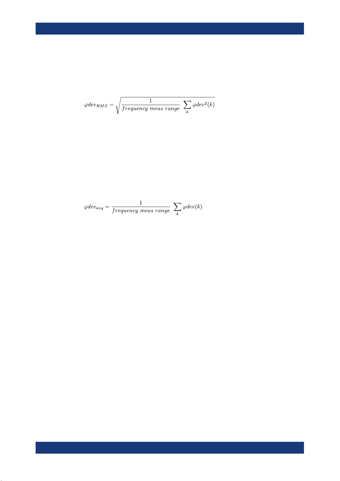
R&S®FSV3-K60
Measurement results
Hop parameters
CALCulate<n>:HOPDetection:TABLe:RESults? on page 358
[SENSe:]HOP:PHASe:MAXPm? on page 372
Phase Deviation (RMS) ← Phase parameters
RMS of Phase Deviation vs Time trace
for k∈ {frequency meas range}
Remote command:
Display:
CALCulate<n>:HOPDetection:TABLe:PHASe:RMSPm on page 262
Results:
CALCulate<n>:HOPDetection:TABLe:RESults? on page 358
[SENSe:]HOP:PHASe:RMSPm? on page 373
Phase Deviation (Average) ← Phase parameters
Average of Phase Deviation vs Time trace
for k∈ {frequency meas range}
Remote command:
Display:
CALCulate<n>:HOPDetection:TABLe:PHASe:AVGPm on page 262
Results:
CALCulate<n>:HOPDetection:TABLe:RESults? on page 358
[SENSe:]HOP:PHASe:AVGPm? on page 372
Power parameters
Hop power parameters
Remote command:
CALCulate<n>:HOPDetection:TABLe:POWer:ALL[:STATe] on page 264
Minimum Power ← Power parameters
Minimum power level measured during a hop. Which part of the hop precisely is used
for calculation depends on the power parameters in the "Power" measurement range
settings (see Chapter 5.7, "Hop / chirp measurement settings", on page 103).
Remote command:
Display:
CALCulate<n>:HOPDetection:TABLe:POWer:MINPower on page 264
Results:
CALCulate<n>:HOPDetection:TABLe:RESults? on page 358
[SENSe:]HOP:POWer:MINPower? on page 379
48User Manual 1179.3280.02 ─ 06
Page 49

R&S®FSV3-K60
Measurement results
Hop parameters
Maximum Power ← Power parameters
Maximum power level measured during a hop. Which part of the hop precisely is used
for calculation depends on the power parameters in the "Power" measurement range
settings (see Chapter 5.7, "Hop / chirp measurement settings", on page 103).
Remote command:
Display:
CALCulate<n>:HOPDetection:TABLe:POWer:MAXPower on page 264
Results:
CALCulate<n>:HOPDetection:TABLe:RESults? on page 358
[SENSe:]HOP:POWer:MAXPower? on page 378
Average Power ← Power parameters
Average power level measured during a hop. Which part of the hop precisely is used
for calculation depends on the power parameters in the "Power" measurement range
settings (see Chapter 5.7, "Hop / chirp measurement settings", on page 103).
Remote command:
Display:
CALCulate<n>:HOPDetection:TABLe:POWer:AVEPower on page 264
Results:
CALCulate<n>:HOPDetection:TABLe:RESults? on page 358
[SENSe:]HOP:POWer:AVEPower? on page 377
Power Ripple ← Power parameters
The power ripple is defined as the ratio of maximum to minimum power inside the
power measurement range of the detected hop (see Chapter 5.7, "Hop / chirp mea-
surement settings", on page 103).
Remote command:
Display:
CALCulate<n>:HOPDetection:TABLe:POWer:PWRRipple on page 264
Results:
CALCulate<n>:HOPDetection:TABLe:RESults? on page 358
[SENSe:]HOP:POWer:MINPower? on page 379
FM settling parameters
FM settling parameters describe the hop when it has settled at the nominal frequency.
For details see Figure 4-3.
Remote command:
CALCulate<n>:HOPDetection:TABLe:FMSettling:ALL[:STATe] on page 259
FM settling point ← FM settling parameters
The FM settling point is the point where FM deviation does not exceed the FM settling
tolerance anymore. Since the signal can pass through the tolerance area several times
while it settles, the actual settling point is determined starting at the center of the hop.
From there, the signal is analyzed backwards until it first leaves the tolerance area.
That is defined as the settling point. One FM settling point is calculated per detected
hop. The FM settling point is provided in seconds (time stamp).
49User Manual 1179.3280.02 ─ 06
Page 50

R&S®FSV3-K60
Measurement results
Hop parameters
Remote command:
Display:
CALCulate<n>:HOPDetection:TABLe:FMSettling:FMSPoint on page 260
Results:
CALCulate<n>:HOPDetection:TABLe:RESults? on page 358
[SENSe:]HOP:FMSettling:FMSPoint? on page 365
FM settling time ← FM settling parameters
The FM settling time refers to the time interval between the detected hop start and the
FM settling point. The FM settling time is determined once per detected hop. The FM
settling time is provided in seconds.
Remote command:
Display:
CALCulate<n>:HOPDetection:TABLe:FMSettling:FMSTime on page 260
Results:
CALCulate<n>:HOPDetection:TABLe:RESults? on page 358
[SENSe:]HOP:FMSettling:FMSTime? on page 366
FM settled length ← FM settling parameters
The FM settled length refers to the duration the signal remains settled around a particular nominal frequency. It is determined as the time interval starting from the FM settling point until the point where the deviation exceeds the settling tolerance (hop end).
The FM settled length is given in seconds.
Remote command:
Display:
CALCulate<n>:HOPDetection:TABLe:FMSettling:FMSLength on page 260
Results:
CALCulate<n>:HOPDetection:TABLe:RESults? on page 358
[SENSe:]HOP:FMSettling:FMSLength? on page 364
PM settling parameters
PM settling parameters describe when the hop has reached its nominal phase value.
For details see Figure 4-3.
Remote command:
CALCulate<n>:HOPDetection:TABLe:PMSettling:ALL[:STATe] on page 263
PM settling point ← PM settling parameters
The PM settling point is the point where FM deviation does not exceed the PM settling
tolerance anymore. Since the signal can pass through the tolerance area several times
while it settles, the actual settling point is determined starting at the center of the hop.
From there, the signal is analyzed backwards until it first leaves the tolerance area.
That is defined as the settling point. One PM settling point is calculated per detected
hop. The PM settling point is provided in seconds (time stamp).
Remote command:
Display:
CALCulate<n>:HOPDetection:TABLe:PMSettling:PMSPoint on page 263
Results:
50User Manual 1179.3280.02 ─ 06
Page 51

R&S®FSV3-K60
Measurement results
Chirp parameters
CALCulate<n>:HOPDetection:TABLe:RESults? on page 358
[SENSe:]HOP:PMSettling:PMSPoint? on page 375
PM settling time ← PM settling parameters
The PM settling time refers to the time interval between the detected hop start and the
PM settling point. The PM settling time is determined once per detected hop. The PM
settling time is provided in seconds.
Remote command:
Display:
CALCulate<n>:HOPDetection:TABLe:PMSettling:PMSTime on page 263
Results:
CALCulate<n>:HOPDetection:TABLe:RESults? on page 358
[SENSe:]HOP:PMSettling:PMSTime? on page 376
PM settled length ← PM settling parameters
The PM settled length refers to the duration the signal remains settled around a particular nominal frequency. It is determined as the time interval starting from the PM settling point until the point where the deviation exceeds the settling tolerance (hop end).
The PM settled length is given in seconds.
Remote command:
Display:
CALCulate<n>:HOPDetection:TABLe:PMSettling:PMSLength on page 263
Results:
CALCulate<n>:HOPDetection:TABLe:RESults? on page 358
[SENSe:]HOP:PMSettling:PMSLength? on page 374
4.2 Chirp parameters
If the additional option R&S FSV/A-K60C is installed, various chirp parameters can be
determined during transient analysis.
The chirp parameters to be measured are very similar to the hop parameters; however,
some values are based on the chirp rather than a frequency, so the resulting unit is Hz/
μs.
The following graphic illustrates the main chirp parameters and characteristic values.
(For a definition of the values used to determine the measured chirp parameters see
Chapter 3.4.2, "Frequency chirping", on page 20.)
51User Manual 1179.3280.02 ─ 06
Page 52

R&S®FSV3-K60
Measurement results
Chirp parameters
Figure 4-6: Definition of the main chirp parameters and characteristic values
In order to obtain these results, select the corresponding parameter in the result configuration (see Chapter 6.2.2, "Table configuration", on page 113) or apply the required
SCPI parameter to the remote command (see Chapter 10.6.5.1, "Chirp results",
on page 247 and Chapter 10.7.2, "Retrieving information on detected chirps",
on page 384).
Settling Parameters
Settling refers to the time it takes the FM or PM signal to remain within a specified tolerance around the nominal frequency.
Settling parameters are calculated from the FM or PM deviation considering the given
FM or PM settling tolerance.
Figure 4-7: Settling parameters for chirped signals
52User Manual 1179.3280.02 ─ 06
Page 53

R&S®FSV3-K60
Measurement results
Chirp parameters
Non-linearity parameters
Non-linearity parameters describe the deviation of the chirped signal frequency in relation to the nominal frequency. The integrated non-linearity defines the deviation in reference to the chirp bandwidth.
Figure 4-8: Non-linearity parameters for chirped signals
Chirp ID and Chirp number
Each individual chirp can be identified by a timestamp which corresponds to the absolute time the beginning of the chirp was detected. In addition, each chirp is provided
with a consecutive number, which starts at 1 for each new measurement. This is useful
to distinguish chirps in a measurement quickly.
Remote commands:
[SENSe:]CHIRp:ID? on page 404
[SENSe:]CHIRp:NUMBer? on page 404
State parameters...........................................................................................................54
└ State Index......................................................................................................54
Timing parameters........................................................................................................ 54
└ Chirp Begin..................................................................................................... 54
└ Chirp Length................................................................................................... 55
└ Chirp Rate.......................................................................................................55
└ Switching Time................................................................................................55
Frequency parameters..................................................................................................55
└ Chirp State Deviation......................................................................................55
└ Average Frequency.........................................................................................56
└ Frequency Deviation (Peak)........................................................................... 56
└ Frequency Deviation (RMS)............................................................................56
└ Frequency Deviation (Average)...................................................................... 57
└ Frequency Overshoot..................................................................................... 57
└ Frequency Undershoot................................................................................... 57
Phase parameters.........................................................................................................57
53User Manual 1179.3280.02 ─ 06
Page 54

R&S®FSV3-K60
Measurement results
Chirp parameters
└ Phase Deviation (Peak).................................................................................. 57
└ Phase Deviation (RMS).................................................................................. 58
└ Phase Deviation (Average).............................................................................58
└ Phase Overshoot............................................................................................ 58
└ Phase Undershoot.......................................................................................... 58
Power parameters.........................................................................................................58
└ Minimum Power.............................................................................................. 59
└ Maximum Power............................................................................................. 59
└ Average Power............................................................................................... 59
└ Power Ripple...................................................................................................59
Frequency non-linearity parameters............................................................................. 59
└ Bandwidth....................................................................................................... 60
└ Frequency INL (Peak).....................................................................................60
└ Frequency INL (RMS).....................................................................................60
└ Frequency INL (Average)................................................................................60
FM settling parameters................................................................................................. 61
└ FM settling point..............................................................................................61
└ FM settling time...............................................................................................61
└ FM settled length............................................................................................ 61
PM settling parameters................................................................................................. 61
└ PM settling point............................................................................................. 62
└ PM settling time.............................................................................................. 62
└ PM settled length............................................................................................ 62
State parameters
Chirp state parameters
Remote command:
CALCulate<n>:CHRDetection:TABLe:STATe:ALL[:STATe] on page 255
State Index ← State parameters
The nominal chirps are numbered consecutively in the "Chirp States" table (see Chap-
ter 5.2.2, "Signal states", on page 77), starting at 0. The state of a detected chirp is
defined as the index of the corresponding nominal chirp frequency.
Remote command:
Display:
CALCulate<n>:CHRDetection:TABLe:STATe:INDex on page 256
Results:
CALCulate<n>:CHRDetection:TABLe:RESults? on page 388
[SENSe:]CHIRp:STATe? on page 414
Timing parameters
Chirp timing parameters
Remote command:
CALCulate<n>:CHRDetection:TABLe:TIMing:ALL[:STATe] on page 256
Chirp Begin ← Timing parameters
Time offset from the analysis region start at which the signal first enters the tolerance
area of a nominal chirp. The tolerance area is defined by the settling tolerance above
and below the defined nominal chirps.
54User Manual 1179.3280.02 ─ 06
Page 55

R&S®FSV3-K60
Measurement results
Chirp parameters
Remote command:
Display:
CALCulate<n>:CHRDetection:TABLe:TIMing:BEGin on page 256
Results:
CALCulate<n>:CHRDetection:TABLe:RESults? on page 388
[SENSe:]CHIRp:TIMing:BEGin? on page 415
Chirp Length ← Timing parameters
The duration of a chirp from begin to end, that is, the time the signal remains in the
tolerance area of a nominal chirp.
Remote command:
Display:
CALCulate<n>:CHRDetection:TABLe:TIMing:LENGth on page 256
Results:
CALCulate<n>:CHRDetection:TABLe:RESults? on page 388
[SENSe:]CHIRp:TIMing:LENGth? on page 416
Chirp Rate ← Timing parameters
Derivative of the FM vs time trace within the frequency measurement range (see Chap-
ter 5.7, "Hop / chirp measurement settings", on page 103).
Remote command:
Display:
CALCulate<n>:CHRDetection:TABLe:TIMing:RATE on page 257
Results:
CALCulate<n>:CHRDetection:TABLe:RESults? on page 388
[SENSe:]CHIRp:TIMing:RATE? on page 416
Switching Time ← Timing parameters
Chirp switching time parameters.
Remote command:
[SENSe:]CHIRp:TIMing:SWITching? on page 417
Frequency parameters
Chirp frequency parameters.
Remote command:
CALCulate<n>:CHRDetection:TABLe:FREQuency:ALL[:STATe] on page 251
Chirp State Deviation ← Frequency parameters
Deviation of the detected chirp rate from the nominal chirp state (in kHz/us).
●
: Average chirp rate estimate obtained from the frequency meas range of a chirp
●
Remote command:
Display:
CALCulate<n>:CHRDetection:TABLe:FREQuency:CHERror on page 252
Results:
: Nominal chirp rate corresponding to detected chirp state
55User Manual 1179.3280.02 ─ 06
Page 56

R&S®FSV3-K60
Measurement results
Chirp parameters
CALCulate<n>:CHRDetection:TABLe:RESults? on page 388
[SENSe:]CHIRp:FREQuency:CHERror? on page 398
Average Frequency ← Frequency parameters
Average frequency measured within the frequency measurement range of the chirp
(see Chapter 5.7, "Hop / chirp measurement settings", on page 103).
Remote command:
Display:
CALCulate<n>:CHRDetection:TABLe:FREQuency:FREQuency on page 252
Results:
CALCulate<n>:CHRDetection:TABLe:RESults? on page 388
[SENSe:]CHIRp:FREQuency:FREQuency? on page 399
Frequency Deviation (Peak) ← Frequency parameters
Maximum of Frequency Deviation vs Time trace.
All chirp frequency deviation table values are calculated from the time domain result:
For chirp start ≤ k ≤ chirp start + chirp length
Where:
f
(k): instantaneous frequency of the measured signal
meas
f
(k): ideal frequency trajectory obtained from weighted quadratic regression of the
ideal
instantaneous signal phase φ
(k) within the frequency measurement range (see
meas
Chapter 5.7, "Hop / chirp measurement settings", on page 103)
The peak deviation is thus defined as:
for k∈ {frequency meas range}
Remote command:
Display:
CALCulate<n>:CHRDetection:TABLe:FREQuency:MAXFm on page 252
Results:
CALCulate<n>:CHRDetection:TABLe:RESults? on page 388
[SENSe:]CHIRp:FREQuency:MAXFm? on page 400
Frequency Deviation (RMS) ← Frequency parameters
for k∈ {frequency meas range}
(fdev is defined in "Frequency Deviation (Peak)" on page 56)
Remote command:
Display:
CALCulate<n>:CHRDetection:TABLe:FREQuency:RMSFm on page 252
Results:
56User Manual 1179.3280.02 ─ 06
Page 57

R&S®FSV3-K60
Measurement results
Chirp parameters
CALCulate<n>:CHRDetection:TABLe:RESults? on page 388
[SENSe:]CHIRp:FREQuency:RMSFm? on page 401
Frequency Deviation (Average) ← Frequency parameters
for k∈ {frequency meas range}
(fdev is defined in "Frequency Deviation (Peak)" on page 56)
Remote command:
Display:
CALCulate<n>:CHRDetection:TABLe:FREQuency:AVGFm on page 251
Results:
CALCulate<n>:CHRDetection:TABLe:RESults? on page 388
[SENSe:]CHIRp:FREQuency:AVGFm? on page 393
Frequency Overshoot ← Frequency parameters
Chirp frequency overshoot parameters.
Remote command:
[SENSe:]CHIRp:FREQuency:OVERshoot? on page 403
Frequency Undershoot ← Frequency parameters
Chirp frequency undershoot parameters.
Remote command:
[SENSe:]CHIRp:FREQuency:UNDershoot? on page 403
Phase parameters
Chirp phase parameters
All chirp phase deviation table values are calculated from the time domain result:
for chirp start ≤ k ≤ chirp start + chirp length
where:
φ
(k): instantaneous phase of the measured signal
meas
φ
(k): ideal phase trajectory obtained from weighted linear regression of
ideal
φ
meas
(k)
within the frequency meas range
Remote command:
CALCulate<n>:CHRDetection:TABLe:PHASe:ALL[:STATe] on page 252
Phase Deviation (Peak) ← Phase parameters
Maximum of Phase Deviation vs Time trace.
The deviation is calculated within the phase measurement range of the hop (see Chap-
ter 5.7, "Hop / chirp measurement settings", on page 103).
for k∈ {frequency meas range}
57User Manual 1179.3280.02 ─ 06
Page 58

R&S®FSV3-K60
Measurement results
Chirp parameters
Remote command:
Display:
CALCulate<n>:CHRDetection:TABLe:PHASe:MAXPm on page 253
Results:
CALCulate<n>:CHRDetection:TABLe:RESults? on page 388
[SENSe:]CHIRp:PHASe:MAXPm? on page 405
Phase Deviation (RMS) ← Phase parameters
RMS of Phase Deviation vs Time trace
for k∈ {frequency meas range}
Remote command:
Display:
CALCulate<n>:CHRDetection:TABLe:PHASe:RMSPm on page 253
Results:
CALCulate<n>:CHRDetection:TABLe:RESults? on page 388
[SENSe:]CHIRp:PHASe:RMSPm? on page 406
Phase Deviation (Average) ← Phase parameters
Average of Phase Deviation vs Time trace
for k∈ {frequency meas range}
Remote command:
Display:
CALCulate<n>:CHRDetection:TABLe:PHASe:AVGPm on page 253
Results:
CALCulate<n>:CHRDetection:TABLe:RESults? on page 388
[SENSe:]CHIRp:PHASe:AVGPm? on page 404
Phase Overshoot ← Phase parameters
Chirp phase overshoot parameters.
Remote command:
[SENSe:]CHIRp:PHASe:OVERshoot? on page 407
Phase Undershoot ← Phase parameters
Chirp phase undershoot parameters.
Remote command:
[SENSe:]CHIRp:PHASe:UNDershoot? on page 407
Power parameters
Chirp power parameters
Remote command:
CALCulate<n>:CHRDetection:TABLe:POWer:ALL[:STATe] on page 254
58User Manual 1179.3280.02 ─ 06
Page 59

R&S®FSV3-K60
Measurement results
Chirp parameters
Minimum Power ← Power parameters
Minimum power level measured during a chirp. Which part of the chirp precisely is
used for calculation depends on the power parameters in the "Power" measurement
range settings (see Chapter 5.7, "Hop / chirp measurement settings", on page 103).
Remote command:
Display:
CALCulate<n>:CHRDetection:TABLe:POWer:MINPower on page 255
Results:
CALCulate<n>:CHRDetection:TABLe:RESults? on page 388
[SENSe:]CHIRp:POWer:MINPower? on page 413
Maximum Power ← Power parameters
Maximum power level measured during a chirp. Which part of the chirp precisely is
used for calculation depends on the power parameters in the "Power" measurement
range settings (see Chapter 5.7, "Hop / chirp measurement settings", on page 103).
Remote command:
Display:
CALCulate<n>:CHRDetection:TABLe:POWer:MAXPower on page 255
Results:
CALCulate<n>:CHRDetection:TABLe:RESults? on page 388
[SENSe:]CHIRp:POWer:MAXPower? on page 412
Average Power ← Power parameters
Average power level measured during a chirp. Which part of the chirp precisely is used
for calculation depends on the power parameters in the "Power" measurement range
configuration (see Chapter 5.7, "Hop / chirp measurement settings", on page 103).
Remote command:
Display:
CALCulate<n>:CHRDetection:TABLe:POWer:AVEPower on page 255
Results:
CALCulate<n>:CHRDetection:TABLe:RESults? on page 388
[SENSe:]CHIRp:POWer:AVEPower? on page 411
Power Ripple ← Power parameters
The power ripple is defined as the ratio of maximum to minimum power inside the
power measurement range of the detected hop (see Chapter 5.7, "Hop / chirp mea-
surement settings", on page 103).
Remote command:
Display:
CALCulate<n>:CHRDetection:TABLe:POWer:PWRRipple on page 255
Results:
CALCulate<n>:CHRDetection:TABLe:RESults? on page 388
[SENSe:]CHIRp:POWer:PWRRipple? on page 413
Frequency non-linearity parameters
Non-linearity parameters describe the deviation of the chirped signal frequency. For
details see Figure 4-8.
59User Manual 1179.3280.02 ─ 06
Page 60

R&S®FSV3-K60
Measurement results
Chirp parameters
Bandwidth ← Frequency non-linearity parameters
The bandwidth describes the frequency range occupied by the chirp.
Remote command:
Display:
CALCulate<n>:CHRDetection:TABLe:FREQuency:BWIDth on page 251
Results:
CALCulate<n>:CHRDetection:TABLe:RESults? on page 388
[SENSe:]CHIRp:FREQuency:BWIDth? on page 397
Frequency INL (Peak) ← Frequency non-linearity parameters
The maximum frequency integrated non-linearity (INL) indicates the maximum deviation of the measured chirp from the nominal chirp, in relation to the chirp bandwidth.
Remote command:
Display:
CALCulate<n>:CHRDetection:TABLe:FREQuency:MAXNonlinear on page 252
Results:
CALCulate<n>:CHRDetection:TABLe:RESults? on page 388
[SENSe:]CHIRp:FREQuency:MAXNonlinear? on page 401
Frequency INL (RMS) ← Frequency non-linearity parameters
The RMS of the frequency integrated non-linearity (INL) indicates the RMS deviation of
the measured chirp from the nominal chirp, in relation to the chirp bandwidth.
Remote command:
Display:
CALCulate<n>:CHRDetection:TABLe:FREQuency:RMSNonlinear on page 252
Results:
CALCulate<n>:CHRDetection:TABLe:RESults? on page 388
[SENSe:]CHIRp:FREQuency:RMSNonlinear? on page 402
Frequency INL (Average) ← Frequency non-linearity parameters
The average integrated non-linearity (INL) indicates the average deviation of the measured chirp from the nominal chirp, in relation to the chirp bandwidth.
Remote command:
Display:
CALCulate<n>:CHRDetection:TABLe:FREQuency:AVGNonlinear on page 252
Results:
CALCulate<n>:CHRDetection:TABLe:RESults? on page 388
[SENSe:]CHIRp:FREQuency:AVGNonlinear? on page 397
60User Manual 1179.3280.02 ─ 06
Page 61

R&S®FSV3-K60
Measurement results
Chirp parameters
FM settling parameters
FM settling parameters describe the chirp when it has reached its nominal frequency
value. For details see Figure 4-7.
Remote command:
CALCulate<n>:CHRDetection:TABLe:FMSettling:ALL[:STATe] on page 250
FM settling point ← FM settling parameters
The FM settling point is the point where FM deviation does not exceed the FM settling
tolerance anymore. Since the signal can pass through the tolerance area several times
while it settles, the actual settling point is determined starting at the center of the chirp.
From there, the signal is analyzed backwards until it first leaves the tolerance area.
That is defined as the settling point. One FM settling point is calculated per detected
chirp. The FM settling point is provided in seconds (time stamp).
Remote command:
Display:
CALCulate<n>:CHRDetection:TABLe:FMSettling:FMSPoint on page 250
Results:
CALCulate<n>:CHRDetection:TABLe:RESults? on page 388
[SENSe:]CHIRp:FMSettling:FMSPoint? on page 394
FM settling time ← FM settling parameters
The FM settling time refers to the time interval between the detected chirp start and the
FM settling point. The FM settling time is determined once per detected chirp. The FM
settling time is provided in seconds.
Remote command:
Display:
CALCulate<n>:CHRDetection:TABLe:FMSettling:FMSTime on page 250
Results:
CALCulate<n>:CHRDetection:TABLe:RESults? on page 388
[SENSe:]CHIRp:FMSettling:FMSTime? on page 395
FM settled length ← FM settling parameters
The FM settled length refers to the duration the signal remains settled around a particular nominal frequency. It is determined as the time interval starting from the FM settling point until the point where the deviation exceeds the settling tolerance (chirp end).
The FM settled length is given in seconds.
Remote command:
Display:
CALCulate<n>:CHRDetection:TABLe:FMSettling:FMSLength on page 250
Results:
CALCulate<n>:CHRDetection:TABLe:RESults? on page 388
[SENSe:]CHIRp:FMSettling:FMSLength? on page 393
PM settling parameters
PM settling parameters describe the chirp when it has reached its nominal phase
value. For details see Figure 4-7.
Remote command:
CALCulate<n>:CHRDetection:TABLe:PMSettling:ALL[:STATe] on page 253
61User Manual 1179.3280.02 ─ 06
Page 62

R&S®FSV3-K60
Measurement results
Evaluation methods for transient analysis
PM settling point ← PM settling parameters
The PM settling point is the point where FM deviation does not exceed the PM settling
tolerance anymore. Since the signal can pass through the tolerance area several times
while it settles, the actual settling point is determined starting at the center of the chirp.
From there, the signal is analyzed backwards until it first leaves the tolerance area.
That is defined as the settling point. One PM settling point is calculated per detected
chirp. The PM settling point is provided in seconds (time stamp).
Remote command:
Display:
CALCulate<n>:CHRDetection:TABLe:PMSettling:PMSPoint on page 254
Results:
CALCulate<n>:CHRDetection:TABLe:RESults? on page 388
[SENSe:]CHIRp:PMSettling:PMSPoint? on page 409
PM settling time ← PM settling parameters
The PM settling time refers to the time interval between the detected chirp start and the
PM settling point. The PM settling time is determined once per detected chirp. The PM
settling time is provided in seconds.
Remote command:
Display:
CALCulate<n>:CHRDetection:TABLe:PMSettling:PMSTime on page 254
Results:
CALCulate<n>:CHRDetection:TABLe:RESults? on page 388
[SENSe:]CHIRp:PMSettling:PMSTime? on page 410
PM settled length ← PM settling parameters
The PM settled length refers to the duration the signal remains settled around a particular nominal frequency. It is determined as the time interval starting from the PM settling point until the point where the deviation exceeds the settling tolerance (chirp end).
The PM settled length is given in seconds.
Remote command:
Display:
CALCulate<n>:CHRDetection:TABLe:PMSettling:PMSLength on page 254
Results:
CALCulate<n>:CHRDetection:TABLe:RESults? on page 388
[SENSe:]CHIRp:PMSettling:PMSLength? on page 408
4.3 Evaluation methods for transient analysis
Access: "Overview" > "Display Config"
The data that was measured by the R&S FSV/A can be evaluated using various different methods, depending on the measurement task.
62User Manual 1179.3280.02 ─ 06
Page 63

R&S®FSV3-K60
Measurement results
Evaluation methods for transient analysis
Table 4-1: Available evaluation methods and evaluation basis
Measurement task Evaluation Evaluation basis
Frequency domain analysis RF Spectrum Full capture buffer
Analysis region
Individual hop / chirp
*)
Time domain analysis RF Power Time Domain
PM Time Domain
FM Time Domain
PM Time Domain (Wrapped)
Chirp Rate Time Domain
I/Q Time Domain
Joint time / frequency analysis Spectrogram Full capture buffer
Demodulation quality analysis Frequency Deviation Time
Signal characteristics
Online I/Q data transfer analysis RF Spectrum
*)
requires additional option R&S FSV/A-K60C/-K60H
*)
Domain
Phase Deviation Time Domain
Hop/Chirp Results Table
Hop/Chirp Statistics Table
Parameter Distribution
Parameter Trend
Spectrogram
RF Power Time Domain
PM Time Domain
FM Time Domain
PM Time Domain (Wrapped)
*)
*)
Full capture buffer
Analysis region
Individual hop / chirp
Analysis region
Individual hop / chirp
Analysis region
Individual hop / chirp
*)
Analysis region
Full capture buffer
*)
*)
All evaluation modes available for Transient Analysis are displayed in the selection bar
in SmartGrid mode.
For details on working with the SmartGrid see the R&S FSV/A Getting Started manual.
By default, the Transient Analysis results are displayed in the following windows:
●
RF Spectrum (full capture buffer)
●
FM Time Domain (analysis region)
●
Spectrogram (full capture buffer)
●
RF Power Time Domain (analysis region)
63User Manual 1179.3280.02 ─ 06
Page 64

R&S®FSV3-K60
Measurement results
Evaluation methods for transient analysis
If the additional options R&S FSV/A-K60C/-K60H are installed, the default result displays are:
●
RF Spectrum (full capture buffer)
●
FM Time Domain (analysis region)
●
Spectrogram (full capture buffer)
●
Frequency Deviation Time Domain (hop/chirp)
●
Hop/Chirp Result Table (analysis region)
The following evaluation methods are available for Transient Analysis:
RF Spectrum.................................................................................................................64
Spectrogram..................................................................................................................65
RF Power Time Domain................................................................................................66
FM Time Domain...........................................................................................................66
I/Q Time Domain...........................................................................................................66
Frequency Deviation Time Domain...............................................................................67
PM Time Domain...........................................................................................................68
PM Time Domain (Wrapped).........................................................................................68
Phase Deviation Time Domain......................................................................................69
Chirp Rate Time Domain...............................................................................................70
Hop/Chirp Results Table............................................................................................... 70
Hop/Chirp Statistics Table.............................................................................................71
Parameter Distribution.................................................................................................. 71
Parameter Trend...........................................................................................................72
Marker Table................................................................................................................. 73
RF Spectrum
The RF Spectrum diagram displays the measured power levels for the detected hops/
chirps. The displayed data corresponds to one particular frame in the spectrogram.
During a running measurement, the most recently captured frame is always displayed.
During analysis, which frame is displayed depends on the selected frame in the spectrogram configuration (see "Select Frame" on page 110) or the marker position in the
spectrogram (see "Frame (for Spectrograms only)" on page 138).
Figure 4-9: RF Spectrum result display
Thus, the RF Spectrum is useful to analyze the input signal measured at a specific
time in more detail.
64User Manual 1179.3280.02 ─ 06
Page 65

R&S®FSV3-K60
Measurement results
Evaluation methods for transient analysis
Detected hops/chirps are indicated by green bars along the x-axis in graphical result
displays. The selected hop/chirp (see "Select Hop / Select Chirp" on page 120) is indicated by a blue bar. The hop/chirp index as displayed in the Hop/Chirp Results Table is
indicated at the bottom of each bar.
In the RF Spectrum for the full capture buffer, the analysis region (AR) is indicated by
vertical blue lines.
Remote command:
LAY:ADD? '1',RIGH, RFSP, see LAYout:ADD[:WINDow]? on page 236
Spectrogram
The spectrogram is a way of displaying multiple consecutive spectra over time. The
power, or more exactly the power level, which is usually displayed over frequency, is
displayed over frequency and time. Thus, joint analysis in the time and frequency
domain is possible.
Graphically, time and frequency represent the vertical and horizontal axes of the diagram. Each coordinate (frequency f, time t) of the diagram is filled with a color representing the level for the respective frequency and time.
At the beginning of a measurement, the diagram is empty. As the measurement advances, the graph is filled line by line from top to bottom. Lines in the spectrogram are
called frames, as each frame represents one spectrum.
As the graph fills from top to bottom, the latest spectrum is always the topmost line,
whereas older frames move towards the bottom. However, older frames that have disappeared from the visible display area can be returned to view by selecting a particular
frame or timestamp.
The frames for each individual sweep are separated by colored lines.
Figure 4-10: Spectrogram of a frequency hopper
Spectrograms are highly configurable. In particular, the number of frames and the colors used to display the power levels can be defined by the user.
Spectrograms are particularly useful in combination with a spectrum display. In this
case, the spectrogram provides an overview of events over time, whereas the spectrum provides details for a specific frame.
For more information on working with spectrograms see Chapter 3.10, "Working with
spectrograms", on page 32.
65User Manual 1179.3280.02 ─ 06
Page 66

R&S®FSV3-K60
Measurement results
Evaluation methods for transient analysis
Remote command:
LAY:ADD? '1',RIGH, SGR, see LAYout:ADD[:WINDow]? on page 236
RF Power Time Domain
Displays the RF power (in dBm) versus time.
The RF Power Time Domain trace is determined as follows:
Remote command:
LAY:ADD? '1',RIGH,RFPT, see LAYout:ADD[:WINDow]? on page 236)
FM Time Domain
Displays the frequency of the demodulated FM signal versus time.
The FM time domain trace is determined as follows:
Remote command:
LAY:ADD? '1',RIGH,FMT, see LAYout:ADD[:WINDow]? on page 236)
I/Q Time Domain
Displays the magnitude of the I and Q components of the demodulated FM signal versus time as separate traces in one diagram.
66User Manual 1179.3280.02 ─ 06
Page 67

R&S®FSV3-K60
Measurement results
Evaluation methods for transient analysis
Remote command:
LAY:ADD:WIND '2',RIGH,IQT see LAYout:ADD[:WINDow]? on page 236
Frequency Deviation Time Domain
Displays the frequency error of the demodulated FM signal versus time.
This display requires additional option R&S FSV/A-K60C/-K60H.
Note: The frequency error is calculated for complete hops/chirps only. Thus, where no
(complete) hops/chirps are available, gaps will occur in the error display.
Figure 4-11: Frequency Deviation Time Domain display with gaps where no (complete) chirps are
detected
67User Manual 1179.3280.02 ─ 06
Page 68

R&S®FSV3-K60
Measurement results
Evaluation methods for transient analysis
The Frequency Deviation for the analysis region in the hop model is calculated as follows:
hop start ≤ k ≤ hop start + dwell time
Where
●
: Average frequency estimate obtained from the frequency meas range of a hop
In the chirp model it is calculated as:
chirp start ≤ k ≤ chirp start + chirp length
Where
●
: Average chirp rate estimate obtained from the frequency meas range of a chirp
●
: Average frequency estimate w.r.t. the chirp center obtained from the frequency
meas range of a chirp
∈
For an individual hop/chirp, k
Remote command:
LAY:ADD? '1',RIGH,FDEV, see LAYout:ADD[:WINDow]? on page 236
Result Range
PM Time Domain
Displays the phase deviations of the demodulated PM signal (in rad or °) versus time.
The PM time domain trace is determined as follows:
Remote command:
LAY:ADD? '1',RIGH,PMT, see LAYout:ADD[:WINDow]? on page 236)
PM Time Domain (Wrapped)
Displays the phase deviations of the wrapped demodulated PM signal (in rad or °) versus time.
68User Manual 1179.3280.02 ─ 06
Page 69

R&S®FSV3-K60
Measurement results
Evaluation methods for transient analysis
Remote command:
LAY:ADD? '1',RIGH,PMWR, see LAYout:ADD[:WINDow]? on page 236
Phase Deviation Time Domain
Displays the phase error of the demodulated PM signal (in rad or °) versus time.
This display requires additional option R&S FSV/A-K60C/-K60H.
Figure 4-12: Phase deviation per chirp over time
Note:
Similar to frequency deviation, the phase error is calculated for complete hops/
chirps only. Thus, where no (complete) hops/chirps are available, gaps will occur in the
error display.
The phase deviation in the hop model is calculated as follows:
With hop state deviation compensation:
Without hop state deviation compensation:
Where:
●
: Average frequency estimate obtained from the frequency meas range of a hop
●
●
●
: Nominal hop frequency corresponding to detected hop state
: Phase offset estimate obtained from the frequency meas range of a hop
t ∈ Result range (for individual hop)
hop start ≤ t ≤ hop start + dwell time (for analysis range)
In the chirp model it is calculated as:
With chirp state deviation compensation:
Without chirp state deviation compensation:
69User Manual 1179.3280.02 ─ 06
Page 70

R&S®FSV3-K60
Measurement results
Evaluation methods for transient analysis
Where:
●
: Average chirp rate estimate obtained from the frequency meas range of a chirp
●
●
: Nominal chirp rate corresponding to detected chirp state
: Average frequency estimate based on the chirp center obtained from the fre-
quency meas range of a chirp
●
: Phase offset estimate obtained from the frequency meas range of a chirp
●
t ∈ Result range (for individual chirp)
chirp start ≤ t ≤ chirp start + chirp length (for analysis range)
Remote command:
LAY:ADD? '1',RIGH,PDEV, see LAYout:ADD[:WINDow]? on page 236
Chirp Rate Time Domain
Displays the chirp rate versus time. This display requires additional option R&S FSV/AK60C/-K60H.
The chirp rate time domain trace is determined as follows:
Remote command:
LAY:ADD? '1',RIGH,CRT, see LAYout:ADD[:WINDow]? on page 236
Hop/Chirp Results Table
Displays the automatically detected hop/chirp parameters in a table of results. This display requires additional option R&S FSV/A-K60C/-K60H.
Which parameters are displayed depends on the "Result Configuration" (see Chap-
ter 6.2.2, "Table configuration", on page 113). The currently selected hop/chirp is high-
lighted blue. The remaining hops/chirps contained in the current capture buffer are
highlighted green.
Figure 4-13: Hop Results Table
70User Manual 1179.3280.02 ─ 06
Page 71

R&S®FSV3-K60
Measurement results
Evaluation methods for transient analysis
For details on the individual parameters see Chapter 4.1, "Hop parameters",
on page 41 or Chapter 4.2, "Chirp parameters", on page 51.
Remote command:
LAY:ADD:WIND '2',RIGH,RTAB see LAYout:ADD[:WINDow]? on page 236
Results:
CALCulate<n>:CHRDetection:TABLe:TOTal? on page 392 / CALCulate<n>:
CHRDetection:TOTal? on page 392
CALCulate<n>:HOPDetection:TABLe:TOTal? on page 363 / CALCulate<n>:
HOPDetection:TOTal? on page 363
Hop/Chirp Statistics Table
Displays statistical values (minimum, maximum, average, standard deviation) for the
measured hop/chirp parameters in a table of results. This display requires additional
option R&S FSV/A-K60C/-K60H.
Both the current capture buffer data and the cumulated captured data from a series of
measurements are evaluated. The statistics computed only from hops/chirps within the
current capture buffer are highlighted green. For reference, the measured parameters
from the Select Hop / Select Chirp are also shown, highlighted blue. The displayed
parameters are the same as in the Hop/Chirp Results Table and can be configured in
the "Result Configuration" (see Chapter 6.2.2, "Table configuration", on page 113).
Figure 4-14: Hop Statistics Table
For details on the individual parameters see Chapter 4.1, "Hop parameters",
on page 41 or Chapter 4.2, "Chirp parameters", on page 51.
Remote command:
LAY:ADD:WIND '2',RIGH,STAB see LAYout:ADD[:WINDow]? on page 236
Parameter Distribution
Plots a histogram of a particular parameter, i.e. all measured parameter values from
the current capture vs hop/chirp count or occurrence in %. Thus you can determine
how often a particular parameter value occurs. For each parameter distribution window
you can configure a different parameter to be displayed.
This evaluation method allows you to distinguish transient and stable effects in a specific parameter, such as a spurious frequency deviation or a fluctuation in power over
several hops.
71User Manual 1179.3280.02 ─ 06
Page 72

R&S®FSV3-K60
Measurement results
Evaluation methods for transient analysis
Note that averaging is not possible for parameter distribution traces.
Remote command:
LAY:ADD:WIND '2',RIGH,PDIS see LAYout:ADD[:WINDow]? on page 236
CALCulate<n>:DISTribution:X? on page 277
CALCulate<n>:DISTribution:Y? on page 277
Chapter 10.6.6, "Configuring parameter distribution displays", on page 267
Parameter Trend
Plots all measured parameter values from the current capture vs another parameter or
the hop/chirp state index. This evaluation allows you to determine trends in a specific
parameter, such as a frequency deviation or a fluctuation in power over several hops.
For each parameter trend window you can configure a different parameter to be displayed for both the x-axis and the y-axis, making this a very powerful and flexible
analysis tool. Note, however, that the same parameter may not be selected on the xaxis and y-axis.
72User Manual 1179.3280.02 ─ 06
Page 73

R&S®FSV3-K60
Measurement results
Evaluation methods for transient analysis
Note that averaging is not possible for parameter trend traces.
Remote command:
LAY:ADD:WIND '2',RIGH,PTR see LAYout:ADD[:WINDow]? on page 236
CALCulate<n>:TRENd:X? on page 278
CALCulate<n>:TRENd:Y? on page 278
Chapter 10.6.7, "Configuring parameter trends", on page 277
Marker Table
Displays a table with the current marker values for the active markers.
This table is displayed automatically if configured accordingly.
Tip: To navigate within long marker tables, simply scroll through the entries with your
finger on the touchscreen.
Remote command:
LAY:ADD? '1',RIGH, MTAB, see LAYout:ADD[:WINDow]? on page 236
Results:
CALCulate<n>:MARKer<m>:X on page 332
CALCulate<n>:MARKer<m>:Y? on page 333
73User Manual 1179.3280.02 ─ 06
Page 74

R&S®FSV3-K60
5 Configuration
Configuration
Configuration overview
Access: [MODE] > "Transient Analysis"
Transient Analysis requires a special application on the R&S FSV/A.
When you switch a measurement channel to the Transient Analysis application the first
time, a set of parameters is passed on from the currently active application. After initial
setup, the parameters for the measurement channel are stored upon exiting and
restored upon re-entering the channel. Thus, you can switch between applications
quickly and easily.
When you activate a measurement channel in the Transient Analysis application, a
Transient measurement for the input signal is started automatically with the default
configuration. The "Meas Config" menu is displayed and provides access to the most
important configuration functions.
Automatic refresh of preview and visualization in dialog boxes after configuration changes
The R&S FSV/A supports you in finding the correct measurement settings quickly and
easily - after each change in settings in dialog boxes, the preview and visualization
areas are updated immediately and automatically to reflect the changes. Thus, you can
see if the setting is appropriate or not before closing the dialog.
● Configuration overview............................................................................................74
● Signal description....................................................................................................76
● Input and frontend settings......................................................................................82
● Trigger settings....................................................................................................... 94
● Data acquisition and analysis region.......................................................................98
● Bandwidth settings................................................................................................101
● Hop / chirp measurement settings........................................................................ 103
● FM video bandwidth..............................................................................................107
● Sweep settings......................................................................................................108
● Adjusting settings automatically............................................................................ 110
5.1 Configuration overview
Access: all menus
Throughout the measurement configuration, an overview of the most important currently defined settings is provided in the "Overview".
74User Manual 1179.3280.02 ─ 06
Page 75

R&S®FSV3-K60
Configuration
Configuration overview
In addition to the main measurement settings, the "Overview" provides quick access to
the main settings dialog boxes. The individual configuration steps are displayed in the
order of the data flow. Thus, you can easily configure an entire measurement channel
from input over processing to output and analysis by stepping through the dialog boxes
as indicated in the "Overview".
In particular, the "Overview" provides quick access to the following configuration dialog
boxes (listed in the recommended order of processing):
1. Signal Description
See Chapter 5.2, "Signal description", on page 76.
2. Input and frontend settings
See Chapter 5.3, "Input and frontend settings", on page 82
3. Triggering
See Chapter 5.4, "Trigger settings", on page 94
4. Data acquisition
See Chapter 5.5, "Data acquisition and analysis region", on page 98
5. Measurement settings
See Chapter 5.7, "Hop / chirp measurement settings", on page 103
6. Analysis
See Chapter 6, "Analysis", on page 111
7. Result configuration
See Chapter 6.2, "Result configuration", on page 111
8. Display configuration
See Chapter 6.1, "Display configuration", on page 111
75User Manual 1179.3280.02 ─ 06
Page 76

R&S®FSV3-K60
Configuration
Signal description
To configure settings
► Select any button to open the corresponding dialog box.
Select a setting in the channel bar (at the top of the measurement channel tab) or
in the diagram footer of a graphical result display to change a specific setting.
For step-by-step instructions on configuring a measurement for Transient Analysis, see
Chapter 7, "How to perform transient analysis", on page 148.
Preset Channel
Select the "Preset Channel" button in the lower left-hand corner of the "Overview" to
restore all measurement settings in the current channel to their default values.
Note: Do not confuse the "Preset Channel" button with the [Preset] key, which restores
the entire instrument to its default values and thus closes all channels on the
R&S FSV/A (except for the default channel)!
Remote command:
SYSTem:PRESet:CHANnel[:EXEC] on page 176
Specific Settings for
The channel can contain several windows for different results. Thus, the settings indicated in the "Overview" and configured in the dialog boxes vary depending on the
selected window.
Select an active window from the "Specific Settings for" selection list that is displayed
in the "Overview" and in all window-specific configuration dialog boxes.
The "Overview" and dialog boxes are updated to indicate the settings for the selected
window.
5.2 Signal description
Access: "Overview" > "Signal Description"
The "Signal Description" settings provide information on the expected signal which can
improve measurement and analysis.
● Signal model........................................................................................................... 76
● Signal states............................................................................................................77
● Timing..................................................................................................................... 81
5.2.1 Signal model
Access: "Overview" > "Signal Description" > "Signal Model" tab
The signal model defines which type of signal to expect (if known), thus determining
the analysis method. These settings are only available if at least one of the additional
options R&S FSV/A-K60C/-K60H are installed.
76User Manual 1179.3280.02 ─ 06
Page 77

R&S®FSV3-K60
5.2.2 Signal states
Configuration
Signal description
Hop Model / Chirp Model
Defines which type of signal to expect (if known), thus determining the analysis
method.
These settings are only available if the additional options R&S FSV/A-K60C/-K60H are
installed.
For more information see Chapter 3.4, "Signal models", on page 18.
"Hop Model"
"Chirp Model"
Remote command:
[SENSe:]SIGNal:MODel on page 199
Access: "Overview" > "Signal Description" > "Signal States" tab
The (nominal) frequencies or chirps the signal is expected to switch to are defined in
advance in the "Signal State" table. Each possible frequency/chirp is considered to be
a hop state/chirp state.These settings are only available if at least one of the additional
options R&S FSV/A-K60C/-K60H are installed.
Signals "hop" between random carrier frequencies in short intervals
The carrier frequency is either increased or decreased linearly over
time.
Figure 5-1: Hop States configuration dialog with additional settings
77User Manual 1179.3280.02 ─ 06
Page 78

R&S®FSV3-K60
Configuration
Signal description
Figure 5-2: Chirp States configuration dialog
For details on the individual parameters see Chapter 3.4.1, "Frequency hopping",
on page 18.
Hop / Chirp Settings......................................................................................................79
Chirp Detection............................................................................................................. 79
Hop / Chirp State Index.................................................................................................79
Frequency Offset / Chirp Rate.......................................................................................79
Tolerance.......................................................................................................................80
Inserting a signal state.................................................................................................. 80
Deleting a signal state...................................................................................................80
Clearing the signal state table.......................................................................................80
Applying changes to the signal state table....................................................................80
Saving the signal state table to a file.............................................................................80
Loading a signal state table from a file..........................................................................80
Generating a series of hop states................................................................................. 80
└ Start Frequency.............................................................................................. 80
└ Step Size.........................................................................................................81
└ No of States.................................................................................................... 81
└ Add to Table....................................................................................................81
78User Manual 1179.3280.02 ─ 06
Page 79

R&S®FSV3-K60
Configuration
Signal description
└ Replace Table................................................................................................. 81
└ Applying a global tolerance value................................................................... 81
└ Applying a global frequency offset..................................................................81
Hop / Chirp Settings
By default, the R&S FSV/A Transient Analysis application performs an automatic hop/
chirp detection according to the measured data. For an initial overview of the signal at
hand this detection is usually sufficient. For more accurate results, particularly if the
input signal is known in advance, the signal states can be adapted as required.
For details see Chapter 3.4.3, "Automatic vs. manual hop/chirp state detection",
on page 21.
Remote command:
CALCulate<n>:CHRDetection:STATes:AUTO on page 201
CALCulate<n>:HOPDetection:STATes:AUTO on page 205
Chirp Detection
Selects the chirp detection mode.
The parameters that can be defined in the chirp state detection table depend on the
chirp settings and the chirp detection mode:
Chirp Detection "On" All parameters are set automati-
Chirp Detection "Off"
Chirp Settings "Auto" Chirp Settings "Manual"
Manual setting of:
●
cally.
Manual setting of:
●
Chirp start
●
Chirp length
Chirp Rate
●
Tolerance
Manual setting of:
●
Chirp start
●
Chirp length
●
Start frequency
●
Stop frequency
Remote command:
CALCulate<n>:CHRDetection:DETection on page 203
Hop / Chirp State Index
The nominal frequency levels are numbered consecutively in the "Hop States"/"Chirp
States" table, starting at 0. A maximum of 1000 states can be defined. The state index
of the corresponding nominal frequency level is assigned to each detected hop/chirp in
the measured signal.
Remote command:
CALCulate<n>:HOPDetection:STATes:NUMBer? on page 206
CALCulate<n>:CHRDetection:STATes:NUMBer? on page 203
CALCulate<n>:HOPDetection:STATes:TABLe:NSTates? on page 207
Frequency Offset / Chirp Rate
The hop states are defined as frequency offsets from the center frequency. Hops are
only detected at these frequencies.
Chirp states are defined as a (linear) chirp rate. Chirps are only detected at these chirp
rates.
79User Manual 1179.3280.02 ─ 06
Page 80

R&S®FSV3-K60
Configuration
Signal description
Remote command:
CALCulate<n>:CHRDetection:STATes[:DATA] on page 202
CALCulate<n>:HOPDetection:STATes[:DATA] on page 205
Tolerance
A tolerance span can be defined to compensate for settling effects in the signal after
switching the frequency. As long as the deviation remains within the tolerance above or
below the nominal frequency, the signal state is detected.
Remote command:
CALCulate<n>:CHRDetection:STATes[:DATA] on page 202
CALCulate<n>:HOPDetection:STATes[:DATA] on page 205
Inserting a signal state
Inserts an additional signal state before the currently selected state.
Deleting a signal state
Deletes the currently selected signal state.
Clearing the signal state table
Deletes all signal states in the signal state table.
Applying changes to the signal state table
Applies the changes to the current signal state table configuration.
Remote command:
CALCulate<n>:HOPDetection:STATes:TABLe:SAVE on page 208
CALCulate<n>:CHRDetection:STATes:TABLe:SAVE on page 203
Saving the signal state table to a file
Saves the current signal state table configuration to a file for later use.
Remote command:
CALCulate<n>:HOPDetection:STATes:TABLe:SAVE on page 208
CALCulate<n>:CHRDetection:STATes:TABLe:SAVE on page 203
Loading a signal state table from a file
Loads the selected signal state table configuration from a file.
Remote command:
CALCulate<n>:HOPDetection:STATes:TABLe:LOAD on page 206
CALCulate<n>:CHRDetection:STATes:TABLe:LOAD on page 203
Generating a series of hop states
For hop signals, additional settings are available which allow you to generate several
regularly spaced hop states very easily and quickly.
These settings are displayed or hidden when you select the "More/Less" button in the
"Signal States" tab of the "Signal Description" dialog box for hop signals.
Start Frequency ← Generating a series of hop states
The frequency at which the first hop state will be generated.
80User Manual 1179.3280.02 ─ 06
Page 81

R&S®FSV3-K60
Configuration
Signal description
Remote command:
CALCulate<n>:HOPDetection:STATes:TABLe:STARt? on page 208
Step Size ← Generating a series of hop states
The distance between two hop states.
Remote command:
CALCulate<n>:HOPDetection:STATes:TABLe:STEP? on page 208
No of States ← Generating a series of hop states
Number of hop states to be generated. A maximum of 1000 states can be defined in
one table.
Remote command:
CALCulate<n>:HOPDetection:STATes:TABLe:NSTates? on page 207
Add to Table ← Generating a series of hop states
Adds the defined number of hop states, starting at the Start Frequency, with the
defined Step Size and a tolerance of 1/2 the Step Size to the existing states in the Hop
States table.
Remote command:
CALCulate<n>:HOPDetection:STATes:TABLe:ADD on page 206
Replace Table ← Generating a series of hop states
Replaces any existing states in the "Hop States" table by the defined number of hop
states, starting at the Start Frequency, with the defined Step Size and a tolerance of
1/2 the Step Size.
Remote command:
CALCulate<n>:HOPDetection:STATes:TABLe:REPLace on page 207
Applying a global tolerance value ← Generating a series of hop states
Applies a global Tolerance value to all hop states in the table at once. By default, a tol-
erance of 1/2 the Step Size is applied when a series of states is generated.
To edit the tolerance value for an individual hop state, select the value directly in the
"Hop States" table and enter the new value.
Remote command:
CALCulate<n>:HOPDetection:STATes:TABLe:TOLerance on page 208
Applying a global frequency offset ← Generating a series of hop states
Applies a global Frequency Offset value to all hop states in the table at once.
To edit the frequency offset for an individual hop state, select the value directly in the
"Hop States" table and enter the new value.
Remote command:
CALCulate<n>:HOPDetection:STATes:TABLe:OFFSet on page 207
5.2.3 Timing
Access: "Overview" > "Signal Description" > "Timing" tab
81User Manual 1179.3280.02 ─ 06
Page 82

R&S®FSV3-K60
Configuration
Input and frontend settings
The dwell time is the time the signal remains in the tolerance area of a nominal hop
frequency, that is, the duration of a hop from beginning to end. A hop/chirp is only
detected if its dwell time lies within the defined minimum and maximum values.
Auto Mode.....................................................................................................................82
Min Dwell Time / Max Dwell Time................................................................................. 82
Auto Mode
If "Auto Mode" is enabled (default), useful dwell time/chirp length limits for the current
measurement are defined automatically.
Otherwise, the manually defined Min Dwell Time / Max Dwell Time values apply.
Remote command:
CALCulate<n>:CHRDetection:LENGth:AUTO on page 200
CALCulate<n>:HOPDetection:DWELl:AUTO on page 204
Min Dwell Time / Max Dwell Time
If "Auto Mode" is disabled, you can define minimum or maximum dwell times, or both,
manually, in order to detect only specific hops, for example.
Remote command:
CALCulate<n>:CHRDetection:LENGth:MAXimum on page 201
CALCulate<n>:CHRDetection:LENGth:MINimum on page 201
CALCulate<n>:HOPDetection:DWELl:MAXimum on page 204
CALCulate<n>:HOPDetection:DWELl:MINimum on page 205
5.3 Input and frontend settings
Access: "Overview" > "Input/Frontend"
The R&S FSV/A can evaluate signals from different input sources and provide various
types of output (such as noise or trigger signals).
The frequency and amplitude settings represent the "frontend" of the measurement
setup.
The output settings are identical to the base unit and are described in the R&S FSV/A
User Manual.
● Input source settings...............................................................................................82
● Output settings........................................................................................................86
● Frequency settings..................................................................................................89
● Amplitude settings...................................................................................................91
5.3.1 Input source settings
Access: "Overview" > "Input/Frontend" > "Input Source" tab
Some settings are also available in the "Amplitude" tab of the "Amplitude" dialog box.
82User Manual 1179.3280.02 ─ 06
Page 83

R&S®FSV3-K60
5.3.1.1 Radio frequency input
Configuration
Input and frontend settings
Input from other sources
The R&S FSV3 Transient Analysis application application can also process input from
the following optional sources:
●
I/Q Input files
●
Active modular probes
● Radio frequency input............................................................................................. 83
● Settings for input from I/Q data files........................................................................85
Access: "Overview" > "Input/Frontend" > "Input Source" tab > "Radio Frequency" tab
The default input source for the R&S FSV/A is the radio frequency. If no additional
options are installed, this is the only available input source.
RF Input Protection
The RF input connector of the R&S FSV/A must be protected against signal levels that
exceed the ranges specified in the data sheet. Therefore, the R&S FSV/A is equipped
with an overload protection mechanism for DC and signal frequencies up to 30 MHz.
This mechanism becomes active as soon as the power at the input mixer exceeds the
specified limit. It ensures that the connection between RF input and input mixer is cut
off.
When the overload protection is activated, an error message is displayed in the status
bar ("INPUT OVLD"), and a message box informs you that the RF input was disconnected. Furthermore, a status bit (bit 3) in the STAT:QUES:POW status register is set.
In this case, you must decrease the level at the RF input connector and then close the
message box. Then measurement is possible again. Reactivating the RF input is also
possible via the remote command INPut<ip>:ATTenuation:PROTection:RESet.
83User Manual 1179.3280.02 ─ 06
Page 84

R&S®FSV3-K60
Configuration
Input and frontend settings
Radio Frequency State................................................................................................. 84
Input Coupling...............................................................................................................84
Impedance.................................................................................................................... 84
Direct Path.................................................................................................................... 84
YIG-Preselector.............................................................................................................85
Radio Frequency State
Activates input from the "RF Input" connector.
Remote command:
INPut<ip>:SELect on page 179
Input Coupling
The RF input of the R&S FSV/A can be coupled by alternating current (AC) or direct
current (DC).
AC coupling blocks any DC voltage from the input signal. AC coupling is activated by
default to prevent damage to the instrument. Very low frequencies in the input signal
can be distorted.
However, some specifications require DC coupling. In this case, you must protect the
instrument from damaging DC input voltages manually. For details, refer to the data
sheet.
Remote command:
INPut<ip>:COUPling on page 178
Impedance
For some measurements, the reference impedance for the measured levels of the
R&S FSV/A can be set to 50 Ω or 75 Ω.
Select 75 Ω if the 50 Ω input impedance is transformed to a higher impedance using a
75 Ω adapter of the RAZ type. (That corresponds to 25Ω in series to the input impedance of the instrument.) The correction value in this case is 1.76 dB = 10 log (75Ω/
50Ω).
Remote command:
INPut<ip>:IMPedance on page 179
Direct Path
Enables or disables the use of the direct path for small frequencies.
In spectrum analyzers, passive analog mixers are used for the first conversion of the
input signal. In such mixers, the LO signal is coupled into the IF path due to its limited
isolation. The coupled LO signal becomes visible at the RF frequency 0 Hz. This effect
is referred to as LO feedthrough.
To avoid the LO feedthrough the spectrum analyzer provides an alternative signal path
to the A/D converter, referred to as the direct path. By default, the direct path is
selected automatically for RF frequencies close to zero. However, this behavior can be
disabled. If "Direct Path" is set to "Off", the spectrum analyzer always uses the analog
mixer path.
"Auto"
(Default) The direct path is used automatically for frequencies close
to zero.
84User Manual 1179.3280.02 ─ 06
Page 85

R&S®FSV3-K60
Configuration
Input and frontend settings
"Off"
Remote command:
INPut<ip>:DPATh on page 178
YIG-Preselector
Enables or disables the YIG-preselector.
This setting requires an additional option on the R&S FSV/A.
An internal YIG-preselector at the input of the R&S FSV/A ensures that image frequen-
cies are rejected. However, image rejection is only possible for a restricted bandwidth.
To use the maximum bandwidth for signal analysis you can disable the YIG-preselector
at the input of the R&S FSV/A, which can lead to image-frequency display.
Note: Note that the YIG-preselector is active only on frequencies greater than
7.5 GHz. Therefore, switching the YIG-preselector on or off has no effect if the frequency is below that value.
To use the optional 54 GHz frequency extension (R&S FSV3-B54G), the YIG-preselector must be disabled.
Remote command:
INPut<ip>:FILTer:YIG[:STATe] on page 179
5.3.1.2 Settings for input from I/Q data files
The analog mixer path is always used.
Access: "Overview" > "Input/Frontend" > "Input Source" > "I/Q File"
Or: [INPUT/OUTPUT] > "Input Source Config" > "Input Source" > "I/Q File"
I/Q Input File State........................................................................................................ 85
Select I/Q data file.........................................................................................................86
I/Q Input File State
Enables input from the selected I/Q input file.
If enabled, the application performs measurements on the data from this file. Thus,
most measurement settings related to data acquisition (attenuation, center frequency,
measurement bandwidth, sample rate) cannot be changed. The measurement time
can only be decreased to perform measurements on an extract of the available data
only.
Note: Even when the file input is disabled, the input file remains selected and can be
enabled again quickly by changing the state.
85User Manual 1179.3280.02 ─ 06
Page 86

R&S®FSV3-K60
Configuration
Input and frontend settings
Remote command:
INPut<ip>:SELect on page 179
Select I/Q data file
Opens a file selection dialog box to select an input file that contains I/Q data.
The I/Q data file must be in one of the following supported formats:
.iq.tar
●
.iqw
●
.csv
●
.mat
●
.wv
●
.aid
●
For details on formats, see the R&S FSV/A I/Q Analyzer and I/Q Input user manual.
Note: Only a single data stream or channel can be used as input, even if multiple
streams or channels are stored in the file.
Note: For some file formats that do not provide the sample rate and measurement time
or record length, you must define these parameters manually. Otherwise the traces are
not visible in the result displays.
The default storage location for I/Q data files is C:\R_S\INSTR\USER.
Remote command:
INPut<ip>:FILE:PATH on page 180
5.3.2 Output settings
Access: "Overview" > "Input/Frontend" > "Output"
or: [INPUT/OUTPUT] > "OUTPUT Config"
The R&S FSV3 Transient Analysis application can provide output to special connectors
for other devices.
For details on connectors, refer to the R&S FSV/A Getting Started manual, "Front /
Rear Panel View" chapters.
Output settings can be configured via the [Input/Output] key or in the "Outputs" dialog
box.
86User Manual 1179.3280.02 ─ 06
Page 87

R&S®FSV3-K60
Configuration
Input and frontend settings
Noise Source Control....................................................................................................87
Trigger 1/2.....................................................................................................................88
└ Output Type.................................................................................................... 88
└ Level..................................................................................................... 89
└ Pulse Length.........................................................................................89
└ Send Trigger.........................................................................................89
Noise Source Control
Enables or disables the 28 V voltage supply for an external noise source connected to
the "Noise source control / Power sensor") connector. By switching the supply voltage
for an external noise source on or off in the firmware, you can enable or disable the
device as required.
External noise sources are useful when you are measuring power levels that fall below
the noise floor of the R&S FSV/A itself, for example when measuring the noise level of
an amplifier.
In this case, you can first connect an external noise source (whose noise power level is
known in advance) to the R&S FSV/A and measure the total noise power. From this
value, you can determine the noise power of the R&S FSV/A. Then when you measure
the power level of the actual DUT, you can deduct the known noise level from the total
power to obtain the power level of the DUT.
Remote command:
DIAGnostic:SERVice:NSOurce on page 181
87User Manual 1179.3280.02 ─ 06
Page 88

R&S®FSV3-K60
Configuration
Input and frontend settings
Trigger 1/2
The trigger input and output functionality depends on how the variable "Trigger Input/
Output" connectors are used.
Note: Providing trigger signals as output is described in detail in the R&S FSV/A User
Manual.
"Trigger 1"
"Trigger 2"
"Trigger 3"
"Input"
"Output"
Remote command:
OUTPut<up>:TRIGger<tp>:DIRection on page 194
Output Type ← Trigger 1/2
Type of signal to be sent to the output
"Output Off"
"Device Triggered"
"Trigger 1" is input only.
Defines the usage of the variable "Trigger Input/Output" connector on
the front panel
Defines the usage of the variable "Trigger 3 Input/Output" connector
on the rear panel
The signal at the connector is used as an external trigger source by
the R&S FSV/A. Trigger input parameters are available in the "Trigger" dialog box.
The R&S FSV/A sends a trigger signal to the output connector to be
used by connected devices.
Further trigger parameters are available for the connector.
Deactivates the output. (Only for "Trigger 3", for which only output is
supported.)
(Default) Sends a trigger when the R&S FSV/A triggers.
88User Manual 1179.3280.02 ─ 06
Page 89

R&S®FSV3-K60
Configuration
Input and frontend settings
"Trigger
Armed"
"User Defined"
Remote command:
OUTPut<up>:TRIGger<tp>:OTYPe on page 195
Level ← Output Type ← Trigger 1/2
Defines whether a high (1) or low (0) constant signal is sent to the trigger output connector (for "Output Type": "User Defined".
The trigger pulse level is always opposite to the constant signal level defined here. For
example, for "Level" = "High", a constant high signal is output to the connector until you
select the Send Trigger function. Then, a low pulse is provided.
Sends a (high level) trigger when the R&S FSV/A is in "Ready for trigger" state.
This state is indicated by a status bit in the STATus:OPERation register (bit 5), as well as by a low-level signal at the "AUX" port (pin 9).
Sends a trigger when you select the "Send Trigger" button.
In this case, further parameters are available for the output signal.
Remote command:
OUTPut<up>:TRIGger<tp>:LEVel on page 194
Pulse Length ← Output Type ← Trigger 1/2
Defines the duration of the pulse (pulse width) sent as a trigger to the output connector.
Remote command:
OUTPut<up>:TRIGger<tp>:PULSe:LENGth on page 196
Send Trigger ← Output Type ← Trigger 1/2
Sends a user-defined trigger to the output connector immediately.
Note that the trigger pulse level is always opposite to the constant signal level defined
by the output Level setting. For example, for "Level" = "High", a constant high signal is
output to the connector until you select the "Send Trigger" function. Then, a low pulse
is sent.
Which pulse level is sent is indicated by a graphic on the button.
Remote command:
OUTPut<up>:TRIGger<tp>:PULSe:IMMediate on page 195
5.3.3 Frequency settings
Access: "Overview" > "Input/Frontend" > "Frequency" tab
89User Manual 1179.3280.02 ─ 06
Page 90

R&S®FSV3-K60
Configuration
Input and frontend settings
Center Frequency......................................................................................................... 90
Center Frequency Stepsize...........................................................................................90
Frequency Offset...........................................................................................................90
Center Frequency
Defines the center frequency of the signal in Hertz.
Remote command:
[SENSe:]FREQuency:CENTer on page 184
Center Frequency Stepsize
Defines the step size by which the center frequency is increased or decreased using
the arrow keys.
The step size can be coupled to another value or it can be manually set to a fixed
value.
"= Center"
"Manual"
Remote command:
[SENSe:]FREQuency:CENTer:STEP on page 184
Frequency Offset
Shifts the displayed frequency range along the x-axis by the defined offset.
This parameter has no effect on the instrument's hardware, on the captured data, or on
data processing. It is simply a manipulation of the final results in which absolute frequency values are displayed. Thus, the x-axis of a spectrum display is shifted by a
constant offset if it shows absolute frequencies. However, if it shows frequencies relative to the signal's center frequency, it is not shifted.
A frequency offset can be used to correct the display of a signal that is slightly distorted
by the measurement setup, for example.
The allowed values range from -1 THz to 1 THz. The default setting is 0 Hz.
Sets the step size to the value of the center frequency. The used
value is indicated in the "Value" field.
Defines a fixed step size for the center frequency. Enter the step size
in the "Value" field.
90User Manual 1179.3280.02 ─ 06
Page 91
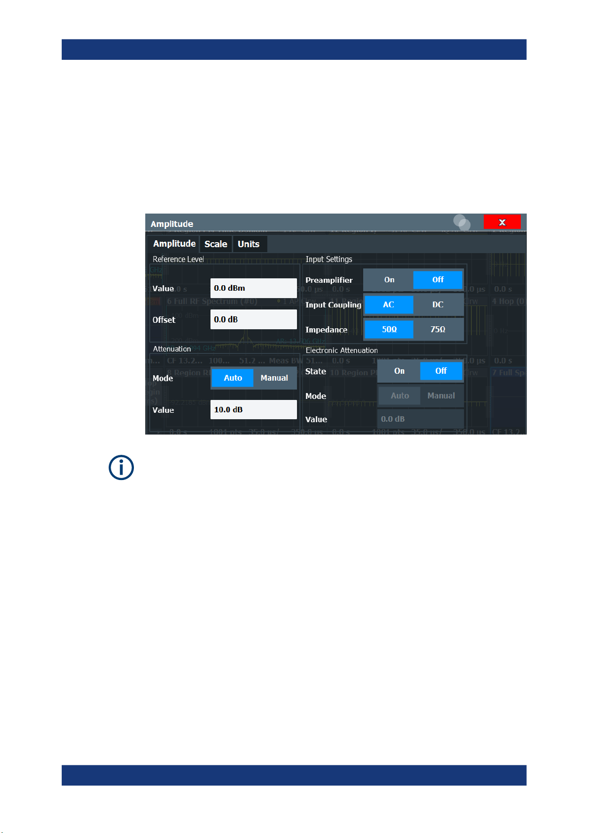
R&S®FSV3-K60
5.3.4 Amplitude settings
Configuration
Input and frontend settings
Remote command:
[SENSe:]FREQuency:OFFSet on page 184
Access: "Overview" > "Input/Frontend" > "Amplitude" tab
Amplitude settings affect the signal power or error levels.
Note that amplitude settings are not window-specific, as opposed to the scaling and
unit settings.
Reference Level............................................................................................................91
└ Shifting the Display (Offset)............................................................................ 92
RF Attenuation.............................................................................................................. 92
└ Attenuation Mode / Value................................................................................92
Using Electronic Attenuation.........................................................................................92
Input Settings................................................................................................................ 93
└ Preamplifier.....................................................................................................93
└ Impedance...................................................................................................... 94
Reference Level
Defines the expected maximum input signal level. Signal levels above this value are
possibly not measured correctly, which is indicated by the "IF Overload" status display.
Defines the expected maximum reference level. Signal levels above this value are possibly not measured correctly. Signals above the reference level are indicated by an "IF
Overload" status display.
The reference level can also be used to scale power diagrams; the reference level is
then used for the calculation of the maximum on the y-axis.
91User Manual 1179.3280.02 ─ 06
Page 92

R&S®FSV3-K60
Configuration
Input and frontend settings
Since the hardware of the R&S FSV/A is adapted according to this value, it is recommended that you set the reference level close above the expected maximum signal
level. Thus you ensure an optimal measurement (no compression, good signal-tonoise ratio).
Remote command:
DISPlay[:WINDow<n>][:SUBWindow<w>]:TRACe<t>:Y[:SCALe]:RLEVel
on page 185
Shifting the Display (Offset) ← Reference Level
Defines an arithmetic level offset. This offset is added to the measured level. In some
result displays, the scaling of the y-axis is changed accordingly.
Define an offset if the signal is attenuated or amplified before it is fed into the
R&S FSV/A so the application shows correct power results. All displayed power level
results are shifted by this value.
The setting range is ±200 dB in 0.01 dB steps.
Note, however, that the internal reference level (used to adjust the hardware settings to
the expected signal) ignores any "Reference Level Offset". Thus, it is important to keep
in mind the actual power level the R&S FSV/A must handle. Do not rely on the displayed reference level (internal reference level = displayed reference level - offset).
Remote command:
DISPlay[:WINDow<n>][:SUBWindow<w>]:TRACe<t>:Y[:SCALe]:RLEVel:
OFFSet on page 186
RF Attenuation
Defines the mechanical attenuation for RF input.
Attenuation Mode / Value ← RF Attenuation
The RF attenuation can be set automatically as a function of the selected reference
level (Auto mode). Automatic attenuation ensures that no overload occurs at the RF
Input connector for the current reference level. It is the default setting.
By default and when no (optional) electronic attenuation is available, mechanical
attenuation is applied.
In "Manual" mode, you can set the RF attenuation in 1 dB steps (down to 0 dB). Other
entries are rounded to the next integer value. The range is specified in the data sheet.
If the defined reference level cannot be set for the defined RF attenuation, the reference level is adjusted accordingly and the warning "limit reached" is displayed.
NOTICE! Risk of hardware damage due to high power levels. When decreasing the
attenuation manually, ensure that the power level does not exceed the maximum level
allowed at the RF input, as an overload can lead to hardware damage.
Remote command:
INPut<ip>:ATTenuation on page 186
INPut<ip>:ATTenuation:AUTO on page 186
Using Electronic Attenuation
If the (optional) Electronic Attenuation hardware is installed on the R&S FSV/A, you
can also activate an electronic attenuator.
92User Manual 1179.3280.02 ─ 06
Page 93

R&S®FSV3-K60
Configuration
Input and frontend settings
In "Auto" mode, the settings are defined automatically; in "Manual" mode, you can
define the mechanical and electronic attenuation separately.
Note: Electronic attenuation is not available for stop frequencies (or center frequencies
in zero span) above 7 GHz.
In "Auto" mode, RF attenuation is provided by the electronic attenuator as much as
possible to reduce the amount of mechanical switching required. Mechanical attenuation can provide a better signal-to-noise ratio, however.
When you switch off electronic attenuation, the RF attenuation is automatically set to
the same mode (auto/manual) as the electronic attenuation was set to. Thus, the RF
attenuation can be set to automatic mode, and the full attenuation is provided by the
mechanical attenuator, if possible.
The electronic attenuation can be varied in 1 dB steps. If the electronic attenuation is
on, the mechanical attenuation can be varied in 5 dB steps. Other entries are rounded
to the next lower integer value.
If the defined reference level cannot be set for the given attenuation, the reference
level is adjusted accordingly and the warning "limit reached" is displayed in the status
bar.
Remote command:
INPut<ip>:EATT:STATe on page 189
INPut<ip>:EATT:AUTO on page 188
INPut<ip>:EATT on page 188
Input Settings
Some input settings affect the measured amplitude of the signal, as well.
For information on other input settings see Chapter 5.3.1.1, "Radio frequency input",
on page 83.
Preamplifier ← Input Settings
If the (optional) internal preamplifier hardware is installed, a preamplifier can be activated for the RF input signal.
You can use a preamplifier to analyze signals from DUTs with low output power.
For R&S FSV/A3004, 3007, 3013, and 3030 models, the following settings are availa-
ble:
"Off"
"15 dB"
"30 dB"
Deactivates the preamplifier.
The RF input signal is amplified by about 15 dB.
The RF input signal is amplified by about 30 dB.
For R&S FSV/A44 or higher models, the input signal is amplified by 30 dB if the preamplifier is activated. In this case, the preamplifier is only available under the following
conditions:
●
In zero span, the maximum center frequency is 43.5 GHz
●
For frequency spans, the maximum stop frequency is 43.5 GHz
●
For I/Q measurements, the maximum center frequency depends on the analysis
bandwidth:
≤
f
43.5 GHz - (<Analysis_bw> / 2)
center
If any of the conditions no longer apply after you change a setting, the preamplifier is
automatically deactivated.
93User Manual 1179.3280.02 ─ 06
Page 94

R&S®FSV3-K60
5.4 Trigger settings
Configuration
Trigger settings
Remote command:
INPut<ip>:GAIN:STATe on page 187
INPut<ip>:GAIN[:VALue] on page 187
Impedance ← Input Settings
For some measurements, the reference impedance for the measured levels of the
R&S FSV/A can be set to 50 Ω or 75 Ω.
Select 75 Ω if the 50 Ω input impedance is transformed to a higher impedance using a
75 Ω adapter of the RAZ type. (That corresponds to 25Ω in series to the input impedance of the instrument.) The correction value in this case is 1.76 dB = 10 log (75Ω/
50Ω).
Remote command:
INPut<ip>:IMPedance on page 179
Access: "Overview" > "Trigger" > "Trigger Source"/"Trigger In/Out"
Trigger settings determine when the input signal is measured. Note that gating is not
available for hop measurements.
When using time domain displays, the position of the trigger signal relative to the trace
is indicated by a vertical red line in the diagram.
External triggers from one of the [TRIGGER INPUT/OUTPUT] connectors on the
R&S FSV/A are configured in a separate tab of the dialog box.
For details see the R&S FSV/A User Manual.
For step-by-step instructions on configuring triggered measurements, see the
R&S FSV/A User Manual.
Trigger Settings.............................................................................................................95
└ Trigger Source................................................................................................ 95
└ Free Run...............................................................................................95
└ External Trigger 1/2.............................................................................. 95
94User Manual 1179.3280.02 ─ 06
Page 95

R&S®FSV3-K60
Configuration
Trigger settings
└ IF Power............................................................................................... 95
└ I/Q Power..............................................................................................96
└ RF Power..............................................................................................96
└ Trigger Level...................................................................................................97
└ Drop-Out Time................................................................................................ 97
└ Trigger Offset..................................................................................................97
└ Slope...............................................................................................................97
└ Hysteresis....................................................................................................... 97
└ Trigger Holdoff................................................................................................ 97
Trigger Settings
The trigger settings define the beginning of a measurement.
Trigger Source ← Trigger Settings
Defines the trigger source. If a trigger source other than "Free Run" is set, "TRG" is
displayed in the channel bar and the trigger source is indicated.
Note: When triggering is activated, the squelch function is automatically disabled.
Remote command:
TRIGger[:SEQuence]:SOURce on page 193
Free Run ← Trigger Source ← Trigger Settings
No trigger source is considered. Data acquisition is started manually or automatically
and continues until stopped explicitly.
Remote command:
TRIG:SOUR IMM, see TRIGger[:SEQuence]:SOURce on page 193
External Trigger 1/2 ← Trigger Source ← Trigger Settings
Data acquisition starts when the TTL signal fed into the specified input connector
meets or exceeds the specified trigger level.
(See "Trigger Level" on page 97).
Note: The "External Trigger 1" softkey automatically selects the trigger signal from the
"Trigger 1 Input / Output" connector on the front panel.
For details, see the "Instrument Tour" chapter in the R&S FSV/A Getting Started man-
ual.
"External Trigger 1"
Trigger signal from the "Trigger 1 Input / Output" connector.
"External Trigger 2"
Trigger signal from the "Trigger 2 Input / Output" connector.
Remote command:
TRIG:SOUR EXT, TRIG:SOUR EXT2
See TRIGger[:SEQuence]:SOURce on page 193
IF Power ← Trigger Source ← Trigger Settings
The R&S FSV/A starts capturing data as soon as the trigger level is exceeded around
the third intermediate frequency.
95User Manual 1179.3280.02 ─ 06
Page 96

R&S®FSV3-K60
Configuration
Trigger settings
For frequency sweeps, the third IF represents the start frequency. The trigger threshold
depends on the defined trigger level, as well as on the RF attenuation and preamplification. A reference level offset, if defined, is also considered. The trigger bandwidth at
the intermediate frequency depends on the RBW and sweep type. For details on available trigger levels and trigger bandwidths, see the instrument data sheet.
For measurements on a fixed frequency (e.g. zero span or I/Q measurements), the
third IF represents the center frequency.
This trigger source is only available for RF input.
The available trigger levels depend on the RF attenuation and preamplification. A refer-
ence level offset, if defined, is also considered.
For details on available trigger levels and trigger bandwidths, see the data sheet.
Remote command:
TRIG:SOUR IFP, see TRIGger[:SEQuence]:SOURce on page 193
I/Q Power ← Trigger Source ← Trigger Settings
If the R&S FSV3-B1000/-B600 bandwidth extension option is active, this trigger is not
available for bandwidths ≥400 MHz.
Triggers the measurement when the magnitude of the sampled I/Q data exceeds the
trigger threshold.
Remote command:
TRIG:SOUR IQP, see TRIGger[:SEQuence]:SOURce on page 193
RF Power ← Trigger Source ← Trigger Settings
Defines triggering of the measurement via signals which are outside the displayed
measurement range.
For this purpose, the instrument uses a level detector at the first intermediate frequency.
The "RF Power" trigger is available for input signals above 500 MHz. The trigger
(6 dB-) bandwidth is ±250 MHz. For the R&S FSV3000 and input signals between
500 MHz and 7.5 GHz, the trigger bandwidth depends on the instrument's serial number, see data sheet.
When using the Direct Path, the RF power trigger is not available.
The resulting trigger level at the RF input depends on the RF attenuation and preampli-
fication. For details on available trigger levels, see the instrument's data sheet.
Note: If the input signal contains frequencies outside of this range (e.g. for fullspan
measurements), the measurement can be aborted. A message indicating the allowed
input frequencies is displayed in the status bar.
A "Trigger Offset", "Trigger Polarity" and "Trigger Holdoff" (to improve the trigger stability) can be defined for the RF trigger, but no "Hysteresis".
If the bandwidth extension option R&S FSV3-B1000/-B600 is active, this trigger is not
available for bandwidths ≥400 MHz.
Remote command:
TRIG:SOUR RFP, see TRIGger[:SEQuence]:SOURce on page 193
96User Manual 1179.3280.02 ─ 06
Page 97

R&S®FSV3-K60
Configuration
Trigger settings
Trigger Level ← Trigger Settings
Defines the trigger level for the specified trigger source.
For details on supported trigger levels, see the instrument data sheet.
Remote command:
TRIGger[:SEQuence]:LEVel[:EXTernal<port>] on page 191
Drop-Out Time ← Trigger Settings
Defines the time that the input signal must stay below the trigger level before triggering
again.
Remote command:
TRIGger[:SEQuence]:DTIMe on page 190
Trigger Offset ← Trigger Settings
Defines the time offset between the trigger event and the start of the measurement.
Offset > 0: Start of the measurement is delayed
Offset < 0: Measurement starts earlier (pretrigger)
Remote command:
TRIGger[:SEQuence]:HOLDoff[:TIME] on page 190
Slope ← Trigger Settings
For all trigger sources except time, you can define whether triggering occurs when the
signal rises to the trigger level or falls down to it.
Remote command:
TRIGger[:SEQuence]:SLOPe on page 193
Hysteresis ← Trigger Settings
Defines the distance in dB to the trigger level that the trigger source must exceed
before a trigger event occurs. Setting a hysteresis avoids unwanted trigger events
caused by noise oscillation around the trigger level.
This setting is only available for "IF Power" trigger sources. The range of the value is
between 3 dB and 50 dB with a step width of 1 dB.
(For details see the R&S FSV/A I/Q Analyzer and I/Q Input User Manual.)
Remote command:
TRIGger[:SEQuence]:IFPower:HYSTeresis on page 191
Trigger Holdoff ← Trigger Settings
Defines the minimum time (in seconds) that must pass between two trigger events.
Trigger events that occur during the holdoff time are ignored.
Remote command:
TRIGger[:SEQuence]:IFPower:HOLDoff on page 190
97User Manual 1179.3280.02 ─ 06
Page 98

R&S®FSV3-K60
5.5 Data acquisition and analysis region
Configuration
Data acquisition and analysis region
Access: "Overview" > "Data Acquisition"
You must define how much and how data is captured from the input signal, and which
part of the captured data is to be analyzed.
For details see Chapter 3.1, "Data acquisition", on page 14.
Measurement Bandwidth.............................................................................................. 98
Sample Rate................................................................................................................. 98
Measurement Time....................................................................................................... 99
Record Length...............................................................................................................99
Long Capture Buffer......................................................................................................99
Analysis Region............................................................................................................ 99
└ Analysis Bandwidth.......................................................................................100
└ Delta Frequency............................................................................................100
└ Time Gate Length......................................................................................... 100
└ Time Gate Start.............................................................................................100
└ Linked analysis bandwidth............................................................................100
└ Linked analysis time span.............................................................................100
└ Visualizing the Analysis Region Parameters (Show Diagram)..................... 100
Measurement Bandwidth
The measurement bandwidth and Sample Rate are interdependent and define the
range of data to be captured. For information on supported sample rates and bandwidths see the data sheet.
Remote command:
[SENSe:]BWIDth:DEMod on page 196
[SENSe:]FREQuency:SPAN on page 197
Sample Rate
The Measurement Bandwidth and sample rate are interdependent and define the
range of data to be captured. For information on supported sample rates and bandwidths see the data sheet.
Remote command:
[SENSe:]SRATe on page 197
98User Manual 1179.3280.02 ─ 06
Page 99

R&S®FSV3-K60
Configuration
Data acquisition and analysis region
Measurement Time
The measurement time and Record Length are interdependent and define the amount
of data to be captured.
The maximum measurement time in the R&S FSV3 Transient Analysis application is
limited only by the available memory ("memory limit reached" message is shown in status bar). Note, however, that increasing the measurement time (and thus reducing the
available memory space) may restrict the number of measurement channels that can
be activated simultaneously on the R&S FSV/A.
Remote command:
[SENSe:]MTIMe on page 197
Record Length
The Measurement Time and record length are interdependent and define the amount
of data to be captured.
The maximum record length in the R&S FSV3 Transient Analysis application is limited
only by the available memory ("memory limit reached" message is shown in status
bar). Note, however, that increasing the record length (and thus reducing the available
memory space) may restrict the number of measurement channels that can be activated simultaneously on the R&S FSV/A.
Remote command:
[SENSe:]RLENgth on page 197
Long Capture Buffer
The long capture buffer provides functionality to use the full I/Q memory depth of the
R&S FSV/A for data acquisition.
The following settings are possible:
●
Off: This is the default setting. Only the standard I/Q memory capacity of the
R&S FSV/A is used. The available I/Q memory capacity is shared by all measurement channels.
●
On: The long capture buffer is activated permanently. A data capture in a different
measurement channel will overwrite and invalidate the acquired I/Q data. A red
"IQ" icon in the channel tab indicates that the results for the channel no longer
match the data currently in the capture buffer.
●
Auto: The long capture buffer is activated in case that the record length exceeds
the amount of data which can be acquired within the standard memory capacity of
the R&S FSV/A. If the record length decreases again, the long capture buffer is
deactivated automatically.
Remote command:
TRACe:IQ:LCAPture on page 198
Analysis Region
The analysis region determines which data is displayed on the screen (see also Chap-
ter 3.6, "Analysis region", on page 22).
The region is defined by a frequency span and a time gate for which the results are
displayed. The time and frequency spans can be defined either as absolute values or
relative to the full capture buffer.
99User Manual 1179.3280.02 ─ 06
Page 100

R&S®FSV3-K60
Configuration
Data acquisition and analysis region
Both methods can be combined, for example by defining an absolute frequency span
and a relative time gate.
Analysis Bandwidth ← Analysis Region
Defines the absolute width of the frequency span for the analysis region. It is centered
around the point defined by the Delta Frequency.
Remote command:
CALCulate<n>:AR:FREQuency:BANDwidth on page 226
Delta Frequency ← Analysis Region
Defines the center of the frequency span for the analysis region. It is defined as an offset from the center frequency.
Remote command:
CALCulate<n>:AR:FREQuency:DELTa on page 226
Time Gate Length ← Analysis Region
Defines the absolute length of the time gate, that is, the duration (or height) of the
analysis region.
Remote command:
CALCulate<n>:AR:TIME:LENGth on page 227
Time Gate Start ← Analysis Region
Defines the starting point of the time span for the analysis region. The starting point is
defined as a time offset from the capture start time.
Remote command:
CALCulate<n>:AR:TIME:STARt on page 228
Linked analysis bandwidth ← Analysis Region
If activated, the width of the frequency span for the analysis region is defined as a percentage of the full capture buffer. It is centered around the point defined by the Delta
Frequency.
Remote command:
CALCulate<n>:AR:FREQuency:PERCent on page 227
CALCulate<n>:AR:FREQuency:PERCent:STATe on page 227
Linked analysis time span ← Analysis Region
If activated, the length of the time gate, that is, the duration (or height) of the analysis
region, is defined as a percentage of the full measurement time. The time gate start is
the start of the capture buffer plus an offset defined by the Time Gate Start.
Remote command:
CALCulate<n>:AR:TIME:PERCent on page 228
CALCulate<n>:AR:TIME:PERCent:STATe on page 228
Visualizing the Analysis Region Parameters (Show Diagram) ← Analysis Region
If enabled, the "Data Acquisition / Analysis Region" dialog box shows a visualization of
the parameters that define the analysis region (as shown in Figure 3-9).
100User Manual 1179.3280.02 ─ 06
 Loading...