Rohde&Schwarz FSV3-K18 User Manual

R&S®FSV3-K18
Power Amplifier and Envelope
Tracking Measurements
User Manual

(;ÜñÜ2)

1178997802
Version 08

This manual applies to the following R&S®FSV3000 and R&S®FSVA3000 models with firmware version

1.90 and higher:

●

R&S®FSV3004 (1330.5000K04) / R&S®FSVA3004 (1330.5000K05)

●

R&S®FSV3007 (1330.5000K07) / R&S®FSVA3007 (1330.5000K08)

●

R&S®FSV3013 (1330.5000K13) / R&S®FSVA3013 (1330.5000K14)

●

R&S®FSV3030 (1330.5000K30) / R&S®FSVA3030 (1330.5000K31)

●

R&S®FSV3044 (1330.5000K43) / R&S®FSVA3044 (1330.5000K44)

●

R&S®FSV3050 (1330.5000K50) / R&S®FSVA3050 (1330.5000K51)

The following firmware options are described:

●

R&S®FSV3-K18 (1346.3347.02)

●

R&S®FSV3-K18D (1346.3353.02)

●

R&S®FSV3-K18F (1346.4408.02)

●

R&S®FSV3-K18M (1345.1486.02)

© 2022 Rohde & Schwarz GmbH & Co. KG
Muehldorfstr. 15, 81671 Muenchen, Germany
Phone: [phone] - 0
Email: [e-mail]
Internet: www.rohde-schwarz.com
Subject to change – data without tolerance limits is not binding.
R&S® is a registered trademark of Rohde & Schwarz GmbH & Co. KG.
Trade names are trademarks of the owners.

1178.9978.02 | Version 08 | R&S®FSV3-K18

The following abbreviations are used throughout this manual: R&S®FSVA3000 is abbreviated as R&S FSVA3000. R&S®FSV3000 is
abbreviated as R&S FSV3000. R&S®FSV/A refers to both the R&S FSV3000 and the R&S FSVA3000. Products of the R&S®SMW
family, e.g. R&S®SMW200A, are abbreviated as R&S SMW.

R&S®FSV3-K18

1 Welcome to the amplifier measurement application.......................... 7

1.1 Starting the application................................................................................................ 7

1.2 Understanding the display information...................................................................... 8

2 Measurements and result displays.................................................... 10

3 Configuration........................................................................................34

3.1 Configuration overview.............................................................................................. 34

3.2 Performing measurements.........................................................................................36

3.3 Designing a reference signal..................................................................................... 37

3.4 Configuring inputs and outputs.................................................................................49

3.4.1 Selecting and configuring the input source................................................................... 49

Contents

Contents

3.4.2 Configuring the frequency............................................................................................. 51

3.4.3 Defining level characteristics.........................................................................................53

3.4.4 Power sensors.............................................................................................................. 56

3.4.5 Using probes................................................................................................................. 61

3.4.6 Configuring outputs....................................................................................................... 61

3.4.7 Controlling a signal generator....................................................................................... 61

3.4.8 Reference: I/Q file input................................................................................................ 66

3.5 Triggering measurements.......................................................................................... 75

3.6 Configuring the data capture..................................................................................... 75

3.7 Sweep configuration...................................................................................................78

3.8 Synchronizing measurement data.............................................................................80

3.9 Evaluating measurement data................................................................................... 83

3.10 Estimating and compensating signal errors............................................................ 85

3.11 Equalizer...................................................................................................................... 86

3.12 Applying system models............................................................................................87

3.13 Applying digital predistortion.................................................................................... 90

3.13.1 Polynomial DPD............................................................................................................ 90

3.13.2 Direct DPD (R&S FSV/A-K18D)....................................................................................93

3.13.3 Memory polynomial DPD (R&S FSV/A-K18M)..............................................................96

3.13.4 Hammerstein model (R&S FSV/A-K18M)..................................................................... 98

3.14 Detailed MSE............................................................................................................. 101

3User Manual 1178.9978.02 ─ 08

R&S®FSV3-K18

3.15 Configuring power measurements..........................................................................103

3.16 Configuring adjacent channel leakage error (ACLR) measurements.................. 104

3.17 Configuring the parameter sweep........................................................................... 106

3.18 Configuring power servoing.................................................................................... 110

4 Analysis...............................................................................................112

4.1 Configuring traces.................................................................................................... 112

4.1.1 Selecting the trace information....................................................................................112

4.1.2 Exporting traces...........................................................................................................115

4.1.3 Detector settings..........................................................................................................116

4.2 Using markers........................................................................................................... 117

4.2.1 Configuring markers.................................................................................................... 117

4.2.2 Configuring individual markers.................................................................................... 118

Contents

4.2.3 Positioning markers.....................................................................................................120

4.3 Customizing numerical result tables...................................................................... 121

4.4 Configuring result display characteristics............................................................. 123

4.5 Scaling the X-Axis.....................................................................................................125

4.6 Scaling the Y-Axis.....................................................................................................127

5 Remote control commands for amplifier measurements...............129

5.1 Introduction............................................................................................................... 129

5.1.1 Conventions used in descriptions............................................................................... 130

5.1.2 Long and short form.................................................................................................... 130

5.1.3 Numeric suffixes..........................................................................................................131

5.1.4 Optional keywords.......................................................................................................131

5.1.5 Alternative keywords................................................................................................... 131

5.1.6 SCPI parameters.........................................................................................................132

5.2 Common suffixes...................................................................................................... 134

5.3 Selecting the application..........................................................................................134

5.4 Configuring the screen layout................................................................................. 138

5.5 Performing amplifier measurements.......................................................................146

5.5.1 Performing measurements..........................................................................................146

5.5.2 Retrieving graphical measurement results..................................................................149

5.5.3 Retrieving numeric results...........................................................................................152

5.5.4 Retrieving I/Q data...................................................................................................... 228

4User Manual 1178.9978.02 ─ 08

R&S®FSV3-K18

5.6 Configuring amplifier measurements..................................................................... 229

5.6.1 Designing a reference signal.......................................................................................230

5.6.2 Selecting and configuring the input source................................................................. 245

5.6.3 Power sensor measurements..................................................................................... 247

5.6.4 Configuring the frequency........................................................................................... 259

5.6.5 Defining level characteristics.......................................................................................260

5.6.6 Controlling a signal generator..................................................................................... 264

5.6.7 Configuring the data capture.......................................................................................274

5.6.8 Sweep configuration....................................................................................................278

5.6.9 Synchronizing measurement data...............................................................................281

5.6.10 Defining the evaluation range..................................................................................... 284

5.6.11 Estimating and compensating signal errors................................................................ 286

5.6.12 Applying a system model............................................................................................ 291

Contents

5.6.13 Applying digital predistortion....................................................................................... 294

5.6.14 Detailed MSE...............................................................................................................311

5.6.15 Configuring ACLR measurements...............................................................................311

5.6.16 Configuring power measurements.............................................................................. 317

5.6.17 Configuring parameter sweeps................................................................................... 318

5.6.18 Configuring power servoing........................................................................................ 322

5.7 Analyzing results...................................................................................................... 325

5.7.1 Configuring traces....................................................................................................... 325

5.7.2 Using markers............................................................................................................. 330

5.7.3 Configuring numerical result displays......................................................................... 341

5.7.4 Configuring the statistics table.................................................................................... 344

5.7.5 Configuring result display characteristics....................................................................345

5.7.6 Scaling the diagram axes............................................................................................350

5.7.7 Managing measurement data..................................................................................... 355

5.8 Deprecated remote commands for amplifier measurements............................... 356

5.9 Programming example R&S FSV/A-K18M.............................................................. 357

List of Commands (Amplifier)...........................................................359

Index....................................................................................................380

5User Manual 1178.9978.02 ─ 08

R&S®FSV3-K18

Contents

6User Manual 1178.9978.02 ─ 08

R&S®FSV3-K18

1 Welcome to the amplifier measurement

Welcome to the amplifier measurement application

Starting the application

application

The R&S FSV3-K18 is a firmware application that adds functionality to measure the
efficiency of amplifiers with the R&S FSV/A signal analyzer. You extend the amplifier
application with the R&S FSV3-K18D, which adds direct DPD functionality.

This user manual contains a description of the functionality that the application pro­vides, including remote control operation.

Functions that are not discussed in this manual are the same as in the base unit and
are described in the R&S FSV/A user manual. The latest versions of the manuals are
available for download at the product homepage.

http://www.rohde-schwarz.com/product/FSV3000.html.

Installation

Find detailed installing instructions in the getting started or the release notes of the
R&S FSV/A.

● Starting the application..............................................................................................7

● Understanding the display information......................................................................8

1.1 Starting the application

The amplifier measurement application adds a new type of measurement to the
R&S FSV/A.

To activate the amplifier application

1. Press the [MODE] key on the front panel of the R&S FSV/A.
A dialog box opens that contains all operating modes and applications currently

available on your R&S FSV/A.

2. Select the "Amplifier" item.

The R&S FSV/A opens a new measurement channel for the amplifier application.
All settings specific to amplifier measurements are in their default state.

7User Manual 1178.9978.02 ─ 08

R&S®FSV3-K18

1.2 Understanding the display information

Welcome to the amplifier measurement application

Understanding the display information

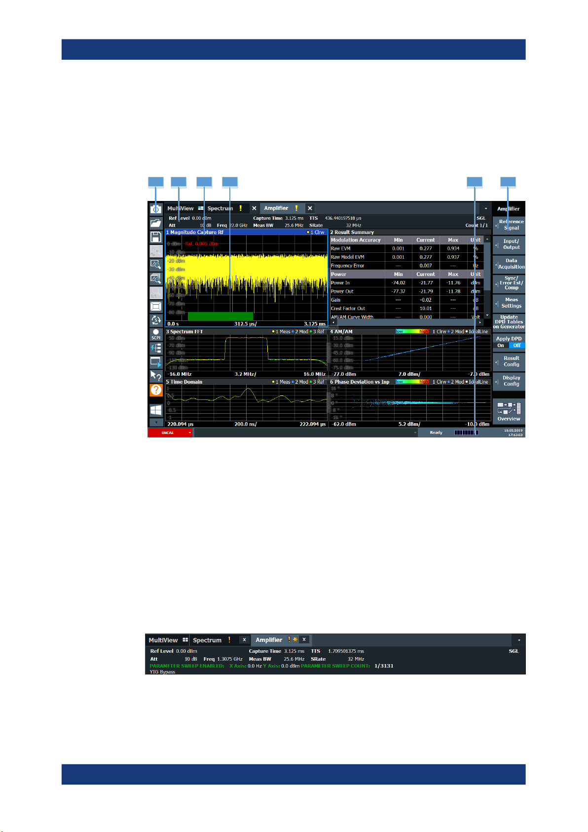
The following figure shows the display as it looks for amplifier measurements. All differ­ent information areas are labeled. They are explained in more detail in the following
sections.

2 3 5 6

1

4

Figure 1-1: Screen layout of the amplifier measurement application

1 = Toolbar
2 = Channel bar
3 = Diagram header
4 = Result display
5 = Status bar
6 = Softkey bar

For a description of the elements not described below, refer to the getting started of the
R&S FSV/A.

Channel bar information

The channel bar contains information about the current measurement setup, progress
and results.

Figure 1-2: Channel bar of the amplifier application

8User Manual 1178.9978.02 ─ 08

R&S®FSV3-K18

Welcome to the amplifier measurement application

Understanding the display information

Ref Level Current reference level of the analyzer.

Att Current attenuation of the analyzer.

Freq Frequency the signal is transmitted on.

Meas Time Length of the signal capture.

Meas BW Bandwidth with which the signal is recorded.

TTF Time difference between the trigger event and the first sample of the reference

signal (= beginning of a frame).

SRate Sample rate with which the signal is recorded.

SGL Indicates that single sweep mode is active.

Count The current signal count for measurement tasks that involve a specific number

of subsequent sweeps (for example the parameter sweep).

X Axis X-axis value that is currently measured.

Y Axis Y-axis value that is currently measured.

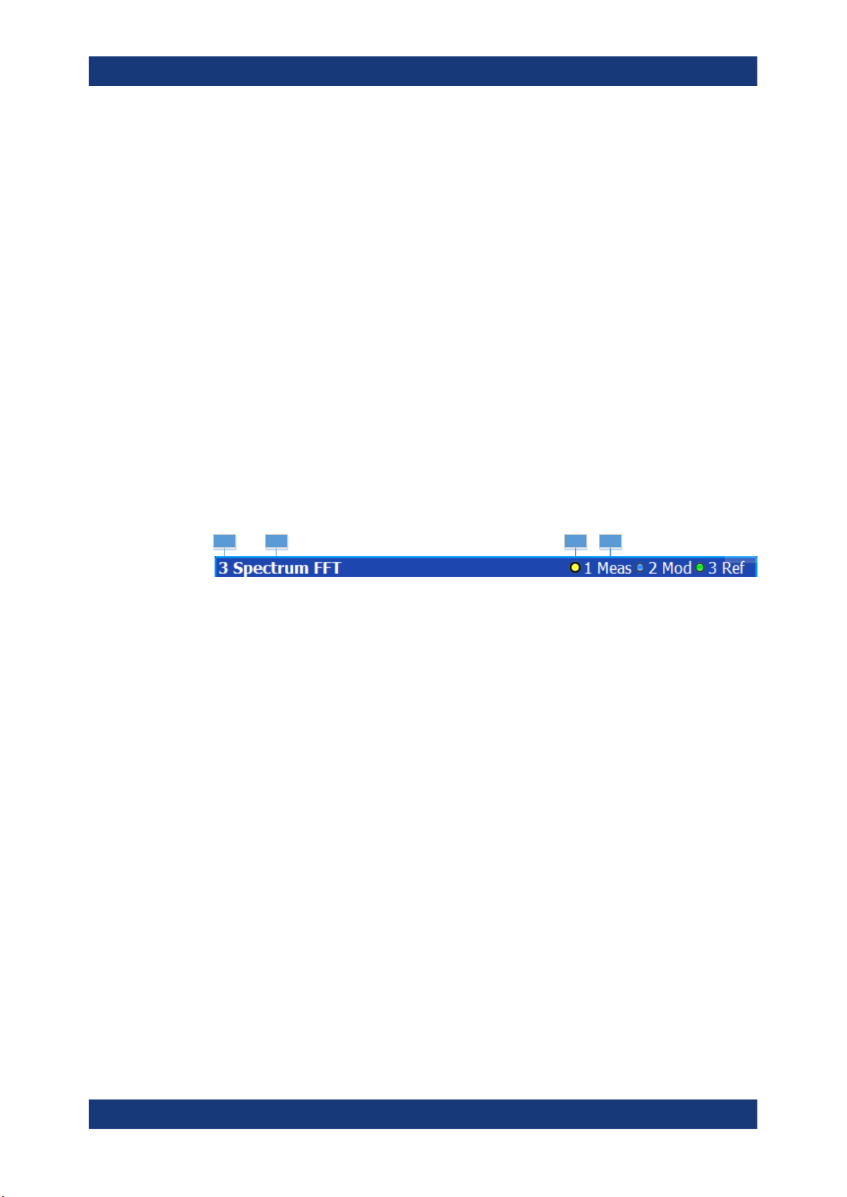
Window title bar information

For each diagram, the header provides the following information:

1

Figure 1-3: Window title bar information of the amplifier application

1 = Window number
2 = Window type
3 = Trace color and number
4 = Trace mode
Blue color = Window is selected

2 3 4

Status bar information

Global instrument settings, the instrument status and any irregularities are indicated in
the status bar beneath the diagram. Furthermore, the progress of the current operation
is displayed in the status bar.

9User Manual 1178.9978.02 ─ 08

R&S®FSV3-K18

2 Measurements and result displays

Measurements and result displays

Note that you can use the R&S FSV3-K18 with the sequencer that is available with the
R&S FSV/A. The functionality is the same as in the spectrum application. Refer to the
R&S FSV/A user manual for more information.

Adjacent Channel Leakage Error (ACLR).....................................................................10

AM/AM...........................................................................................................................11

AM/PM.......................................................................................................................... 12

Channel Response Magnitude / Channel Response Phase / Group Delay (R&S FSV/A-

K18F)............................................................................................................................ 13

DDPD Results (R&S FSV/A-K18D)...............................................................................15

EVM vs Power...............................................................................................................16

Error Vector Spectrum...................................................................................................17

Gain Compression........................................................................................................ 17

Gain Deviation vs Time.................................................................................................19

Magnitude Capture........................................................................................................19

Memory DPD Coefficients.............................................................................................20

Parameter Sweep......................................................................................................... 20

└ Parameter Sweep: Diagram............................................................................20

└ Parameter Sweep: Table.................................................................................21

Phase Deviation vs Time...............................................................................................22

Raw EVM...................................................................................................................... 22

Numeric Result Summary............................................................................................. 23

└ Results to check modulation accuracy............................................................25

└ Results to check power characteristics...........................................................28

Spectrum FFT............................................................................................................... 30

Time Domain.................................................................................................................31

└ Scale of the x-axis (display settings for the time domain)...............................31

└ Scale of the y-axis (display settings for the time domain)...............................32

Statistics Table.............................................................................................................. 32

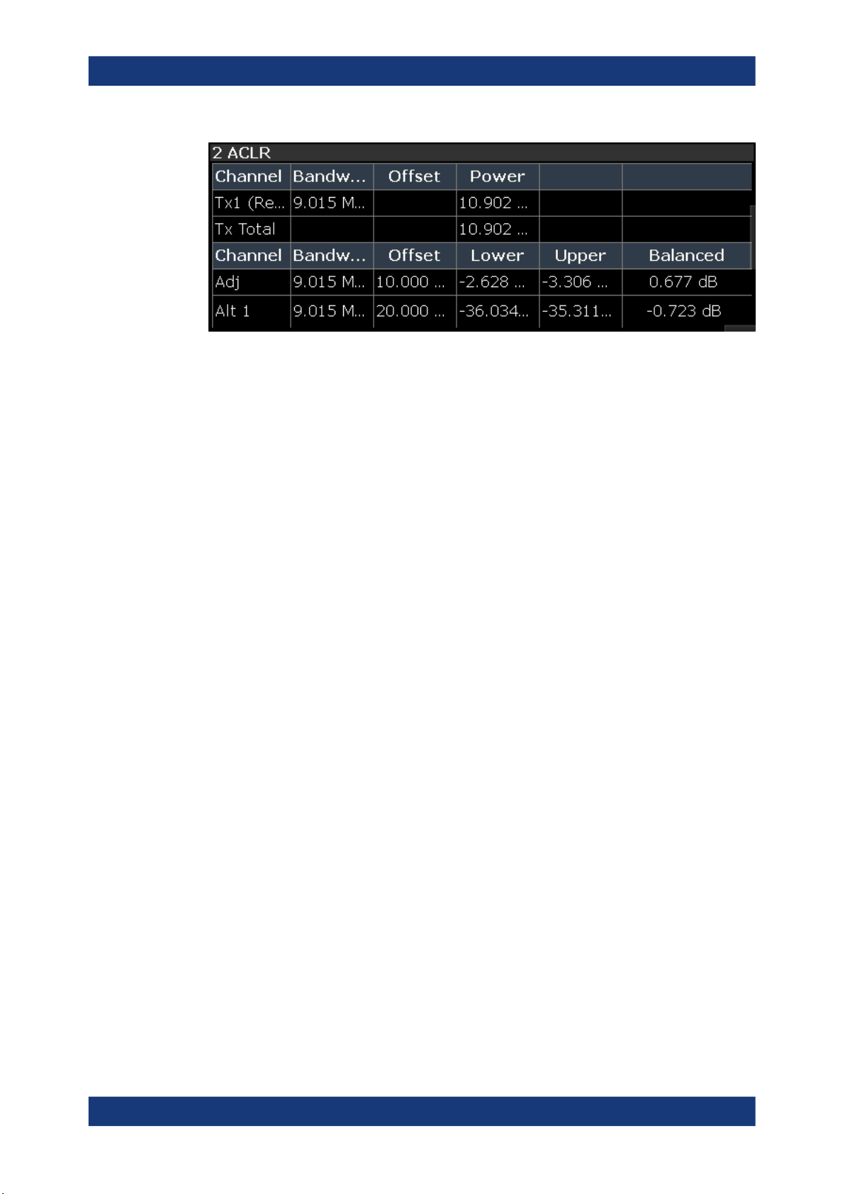
Adjacent Channel Leakage Error (ACLR)

The "ACLR" result display shows the power characteristics of the transmission (Tx)
channel and its neighboring channel(s).

The ACLR measurement in the R&S FSV3-K18 is a measurement based on I/Q data.
Thus, its results are calculated by the same I/Q data as the rest of the results (like the
EVM). Note that the supported channel bandwidth is limited by the I/Q bandwidth of the
analyzer you are using.

The results are provided in numerical form in a table. The table is made up out of two
parts, one part containing the characteristics of the Tx channel, the other containing
those of the neighboring channels.

10User Manual 1178.9978.02 ─ 08

R&S®FSV3-K18

Measurements and result displays

The table contains the following information.

●

Channel

Shows the type of channel.

●

Bandwidth

Shows the channel's bandwidth.

●

Offset (neighboring channels only)
Shows the frequency offset between the center frequency of the adjacent (or alter­nate) channel and the center frequency of the transmission channel.

●

Power

Shows the power of the transmission channel, or the power of the upper / lower
neighboring channel.
The result is calculated over the complete capture buffer, not just the evaluation
range.

●

Balanced

Shows the difference between the lower and upper adjacent channel power
("Lower Channel" - "Upper Channel").

For more information on configuring the ACP measurement, see Chapter 3.16, "Con-

figuring adjacent channel leakage error (ACLR) measurements", on page 104.

Remote command:
Selection: LAY:ADD? '1',LEFT,ACP
Result query: CALCulate<n>:MARKer<m>:FUNCtion:POWer:RESult?
on page 312

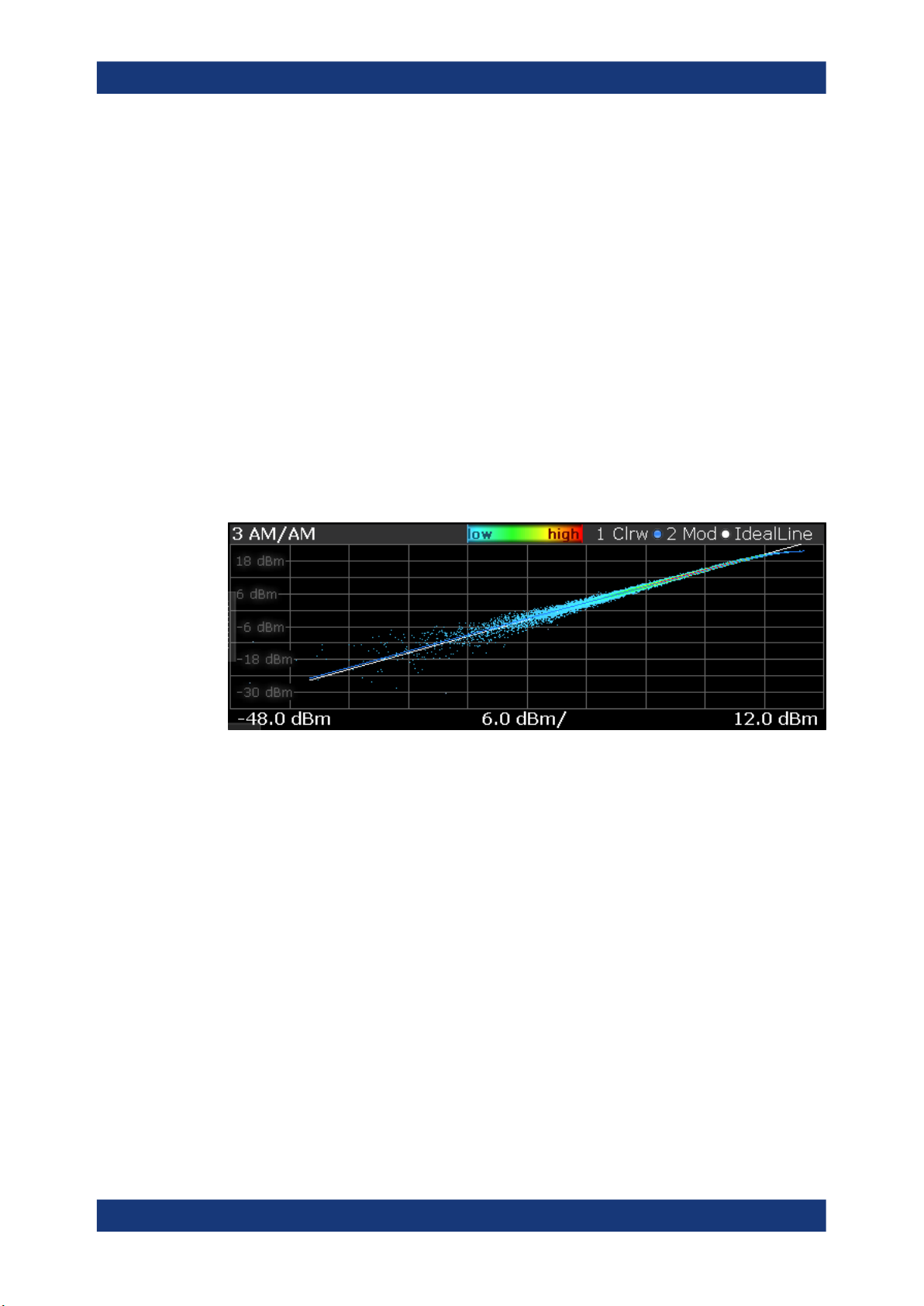
AM/AM

The "AM/AM" result display shows nonlinear effects of the DUT. It shows the amplitude
at the DUT input against the amplitude at the DUT output.

The ideal "AM/AM" curve would be a straight line at 45°. However, nonlinear effects
result in a measurement curve that does not follow the ideal curve. When you drive the
amplifier into saturation, the curve typically flattens at high input levels.

The width of the "AM/AM" trace is an indicator of memory effects: the larger the width
of the trace, the more memory effects occur. The "AM/AM" Curve Width is shown in the
numerical Result Summary.

Both axes show the power of the signal in dBm.
You can analyze the "AM/AM" characteristics of the measured signal and the modeled

signal.

●

Measured signal

11User Manual 1178.9978.02 ─ 08

R&S®FSV3-K18

Measurements and result displays

Shows the "AM/AM" characteristics of the DUT.
The software uses the reference signal in combination with the synchronized mea­surement signal to calculate a software model that describes the characteristics of
the device under test.
The measured signal is represented by a colored cloud of values. The cloud is
based on the recorded samples. If samples have the same values (and would thus
be superimposed), colors represent the statistical frequency with which a certain
input / output level combination occurs. Blue pixels represent low statistical fre­quencies, red pixels high statistical frequencies. A color map is provided within the
result display.

●

Modeled signal
Shows the "AM/AM" characteristics of the model that has been calculated. The
modeled signal is calculated by applying the DUT model to the reference signal.
When the model matches the characteristics of the DUT, the characteristics of the
model signal are the same as those of the measured signal (minus noise).
The modeled signal is represented by a line trace.
When system modeling has been turned off, this trace is not displayed.

All traces include the digital predistortion, when you have turned on that feature.

Remote command:
Selection: LAY:ADD? '1',LEFT,AMAM
Result query: TRACe<n>[:DATA]? on page 150

AM/PM

The "AM/PM" result display shows nonlinear effects of the DUT. It shows the phase dif­ference between DUT input and output for each sample of the synchronized measure­ment signal.

The ideal "AM/PM" curve would be a straight line at 0°. However, nonlinear effects
result in a measurement curve that does not follow the ideal curve. Typically, the curve
drifts from a zero phase shift, especially at high power levels when you drive the ampli­fier into saturation.

The width of the "AM/PM" trace is an indicator of memory effects: the larger the width
of the trace, the more memory effects occur. The "AM/PM" curve width is shown in the
numerical Result Summary.

The x-axis shows the levels of all samples of the reference signal (input power) or the
measurement signal (output power) in dBm. You can select the reference of the x-axis
(input or output power) in the "Result Configuration" dialog box.

12User Manual 1178.9978.02 ─ 08

R&S®FSV3-K18

Measurements and result displays

The y-axis shows the phase of the signal for the corresponding power level. The unit is
either rad or degree, depending on your phase unit selection in the "Result Configura­tion" dialog box.

You can analyze the "AM/PM" characteristics of the real DUT or of the modeled DUT.

●

Measured signal
Shows the "AM/PM" characteristics of the DUT.
The software uses the reference signal together with the synchronized measure­ment signal to calculate a software model that describes the characteristics of the
device under test.
The measured signal is represented by a colored cloud of values. The cloud is
based on the recorded samples. If samples have the same values (and would thus
be superimposed), colors represent the statistical frequency with which a certain
input / output level combination occurs. A color map is provided within the result
display.

●

Modeled signal
Shows the "AM/PM" characteristics of the model that has been calculated. The
modeled signal is calculated by applying the DUT model to the reference signal.
When the model matches the characteristics of the DUT, the characteristics of the
modeled signal are the same as those of the measured signal (minus noise).
The modeled signal is represented by a line trace.
When system modeling has been turned off, this trace is not displayed.

All traces include the digital predistortion, when you have turned on that feature.

Remote command:
Selection: LAY:ADD? '1',LEFT,AMPM
Result query: TRACe<n>[:DATA]? on page 150

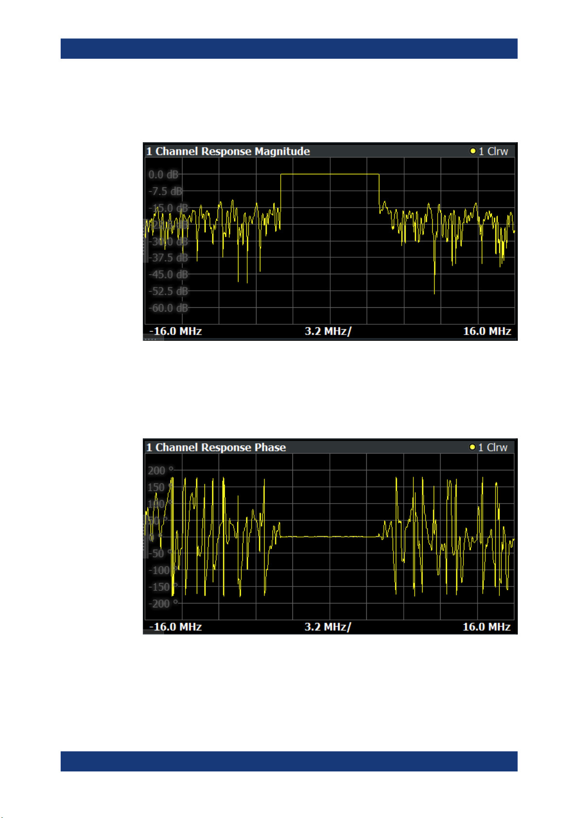
Channel Response Magnitude / Channel Response Phase / Group Delay
(R&S FSV/A-K18F)

The channel response and group delay result displays show the deviation of the mea­sured signal compared to the reference signal within the measured channel. The result
displays contain a single trace.

Outside of the occupied bandwidth, the reference signal values usually lie below the
measured noise floor. This can result in large peaks on the trace in these areas (usu­ally to the left and right of the channel). Note that because of the automatic y-axis scal-

ing, the trace can appear in parts as a straight horizontal line. In that case, adjust the

scale of the y-axis manually.

13User Manual 1178.9978.02 ─ 08

R&S®FSV3-K18

Measurements and result displays

Channel Response Magnitude

The "Channel Response Magnitude" result display analyzes the magnitude character­istics of the signal over the measurement bandwidth.

For the "Channel Response Magnitude", the y-axis shows the deviation of the mea­sured magnitude relative to the transmitted signal power of the signal generator in dB.
The x-axis shows the frequency over which the signal was measured.

Channel Response Phase

The "Channel Response Phase" result display analyzes the phase characteristics of
the signal over the measurement bandwidth.

For the "Channel Response Phase", the y-axis shows the phase deviation relative to
the reference signal. The unit depends on your selection. The x-axis shows the fre­quency over which the signal was measured.

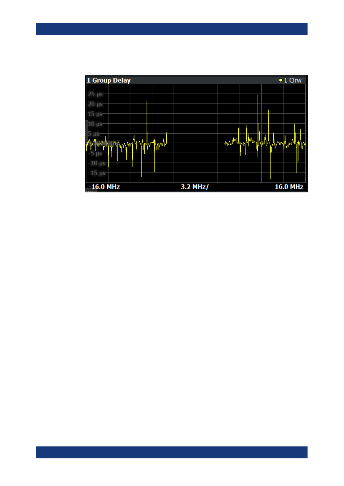
Group Delay

14User Manual 1178.9978.02 ─ 08

R&S®FSV3-K18

Measurements and result displays

The "Group Delay" result display analyzes the relative group delay of the signal over
the measurement bandwidth.

For the "Group Delay", the y-axis shows the measured time delay relative to the refer­ence signal in seconds. The x-axis shows the frequency over which the signal was
measured.

Remote command:
Selection (magnitude): LAY:ADD? '1',LEFT,MRES
Selection (phase): LAY:ADD? '1',LEFT,PRES
Selection (group delay): LAY:ADD? '1',LEFT,GDEL
Result query: TRACe<n>[:DATA]? on page 150

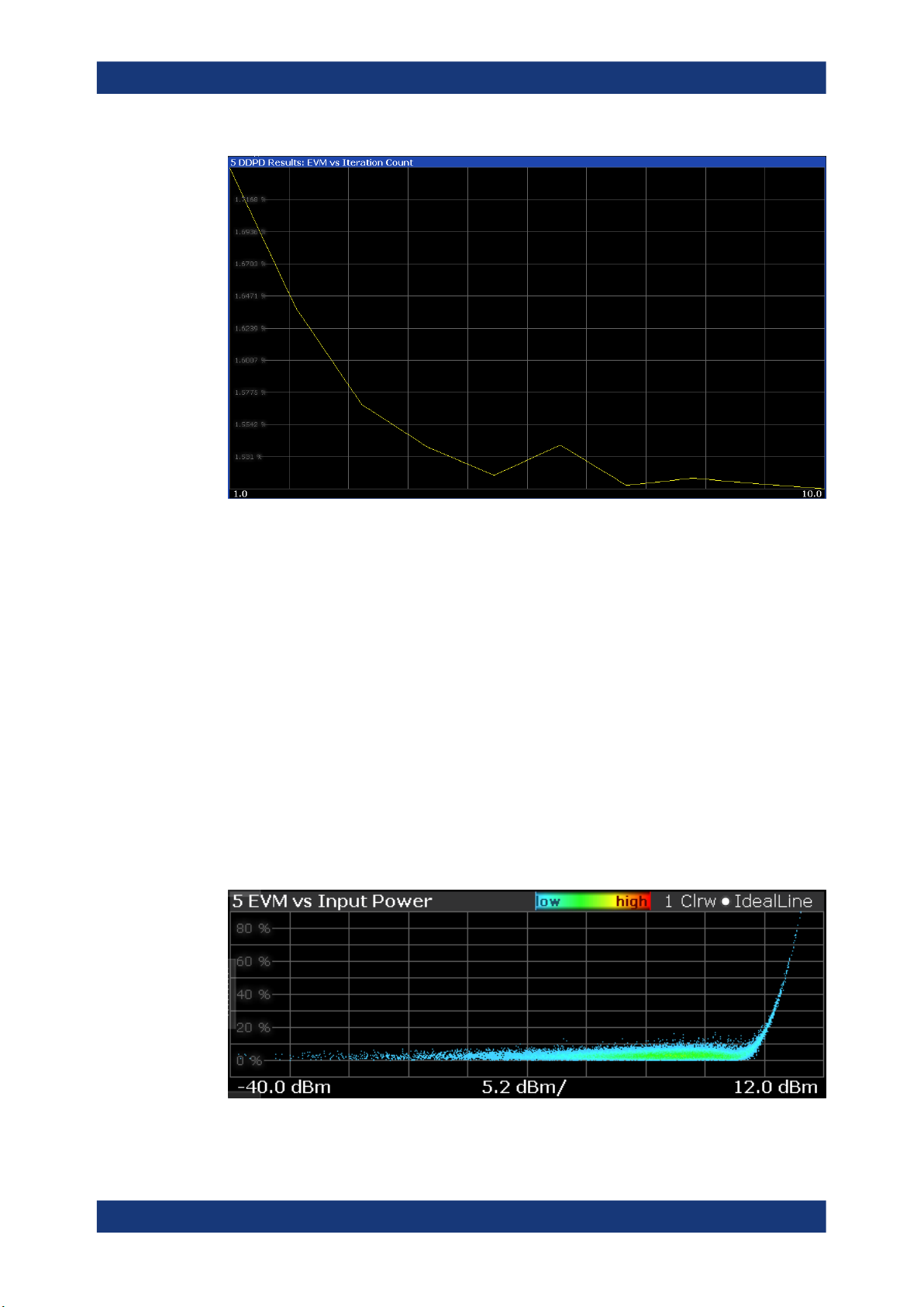
DDPD Results (R&S FSV/A-K18D)

The "DDPD Results" result display shows a selectable result (such as EVM or ACLR)
over all iterations of the direct DPD. This allows verification of the direct DPD's conver­gence as well as picking the ideal iteration step for further processing (e.g. in
R&S FSV/A-K18M). It is only available with application R&S FSV/A-K18D installed.

The display must be placed on screen before starting the direct DPD. The result type is
configurable in the "Result Configuration" dialog box.

15User Manual 1178.9978.02 ─ 08

R&S®FSV3-K18

Measurements and result displays

Remote command:
Selection: LAY:ADD? '1',LEFT,DDPD
Configure result type: CONFigure:DDPD:WINDow<n>:RESult on page 299
Result query: TRACe<n>[:DATA]? on page 150

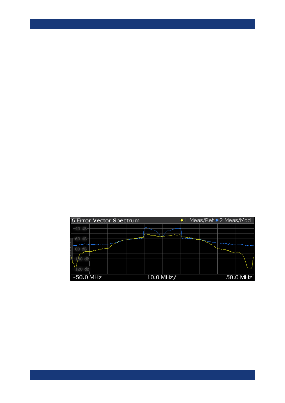
EVM vs Power

The "EVM vs Power" result display shows the EVM against the measured power val­ues.

The ideal EVM vs power curve would be a straight line at 0 %. However, among other
effects such as noise, nonlinear effects of the DUT cause an increase of the EVM.
Nonlinear effects usually occur on high power levels that drive the power amplifier into
saturation.

The x-axis shows the levels of all samples of the reference signal (input power) or the
measurement signal (output power) in dBm. You can select the reference of the x-axis
(input or output power) in the "Result Configuration" dialog box.

The y-axis shows the EVM of the signal for the corresponding power level in %.
All traces include the digital predistortion, when you have turned on that feature.

16User Manual 1178.9978.02 ─ 08

R&S®FSV3-K18

Measurements and result displays

Remote command:
Selection: LAY:ADD? '1',LEFT,AMEV
Result query: TRACe<n>[:DATA]? on page 150

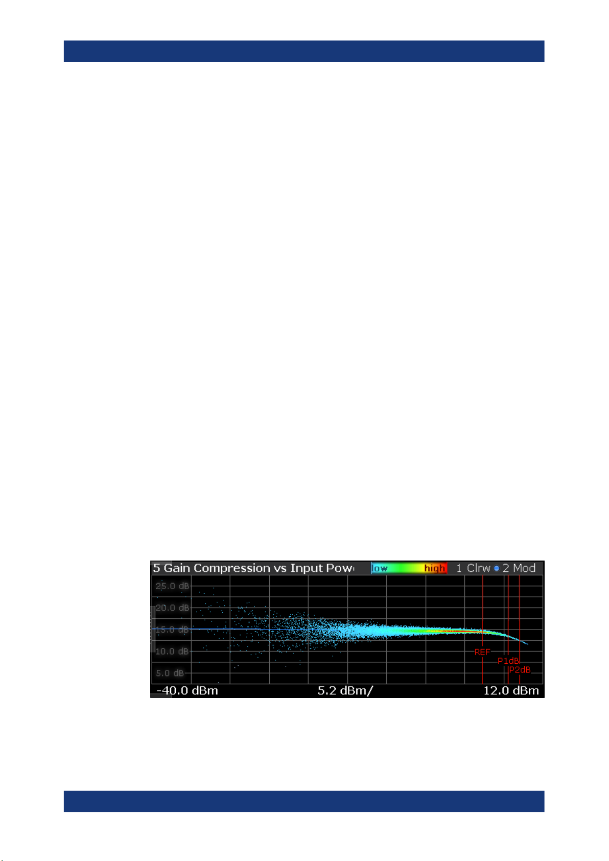
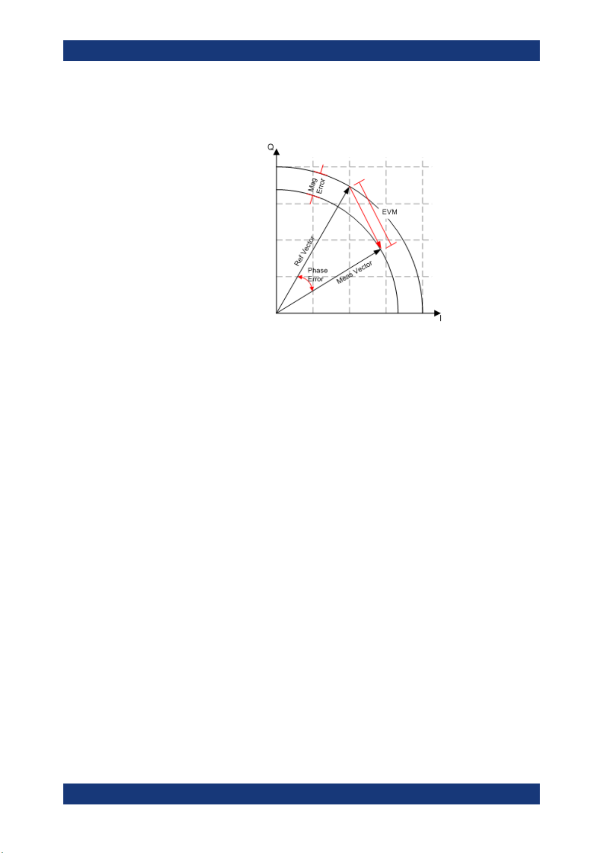
Error Vector Spectrum

The "Error Vector Spectrum" result display shows the error vector (EV) signal in the
spectrum around the center frequency.

The EV is a measure of the modulation accuracy. It compares two signals and shows
the distance of the measured constellation points and the ideal constellation points.

The unit is dB.
You can compare the measured signal against the reference signal and against the

modeled signal.

●

Measured signal against reference signal
Trace 1 compares measured signal and the reference signal.
To get useful results, the calculated linear gain is compensated to match both sig­nals.
Depending on the DUT, noise and nonlinear effects may have been added to the
measurement signal. These effects are visualized by this trace.

●

Measured signal against modeled signal
Trace 2 compares measured signal and the modeled signal.
The EVM between the measured and modeled signal indicates the quality of the
DUT modeling. If the model matches the DUT behavior, the modeling error is zero
(or is merely influenced by noise).
This result display shows changes in the model and its parameters and thus allows
you to optimize the modeling.
When system modeling has been turned off, this trace is not displayed.

Remote command:
Selection: LAY:ADD? '1',LEFT,SEVM
Result query: TRACe<n>[:DATA]? on page 150

Gain Compression

The "Gain Compression" result display shows the gain and error effects of the DUT
against the DUT input or output power.

The gain is the ratio of the input and output power of the DUT.

17User Manual 1178.9978.02 ─ 08

R&S®FSV3-K18

Measurements and result displays

The x-axis shows the levels of all samples of the reference signal (input power) or the
measurement signal (output power) in dBm. You can select the reference of the x-axis
(input or output power) in the "Result Configuration" dialog box.

The y-axis shows the gain in dB.
The ideal gain compression curve would be a straight horizontal line. However, nonlin-

ear effects result in a measurement curve that does not follow the ideal curve. In addi­tion, the curve widens at very low input levels due to noise influence.

The width of the gain compression trace is an indicator of memory effects: the larger
the width of the trace, the more memory effects occur.

You can analyze the gain characteristics of the measured signal and the modeled sig­nal.

●

Measured signal
Shows the gain characteristics of the DUT.
The software uses the reference signal in combination with the synchronized mea­surement signal to calculate a software model that describes the characteristics of
the device under test.
The measured gain is represented by a colored cloud of values. The cloud is
based on the recorded samples. If samples have the same values (and would thus
be superimposed), colors represent the statistical frequency with which a certain
input / output level combination occurs. Blue pixels represent low statistical fre­quencies, red pixels high statistical frequencies. A color map is provided within the
result display.

●

Modeled signal
Shows the gain characteristics of the model that has been calculated. The modeled
signal is calculated by applying the DUT model to the reference signal.
When the model matches the characteristics of the DUT, the characteristics of the
model signal are the same as those of the measured signal (minus noise).
The modeled signal is represented by a line trace.
When system modeling has been turned off, this trace is not displayed.

In addition, one or more horizontal lines can appear in the result display.

●

One line to indicate each compression point (1 dB, 2 dB and 3 dB).

●

One line to indicate the reference point (0 dB compression) that the compression
points refer to.

Remote command:
Selection: LAY:ADD? '1',LEFT,GC
Result query: TRACe<n>[:DATA]? on page 150

18User Manual 1178.9978.02 ─ 08

R&S®FSV3-K18

Measurements and result displays

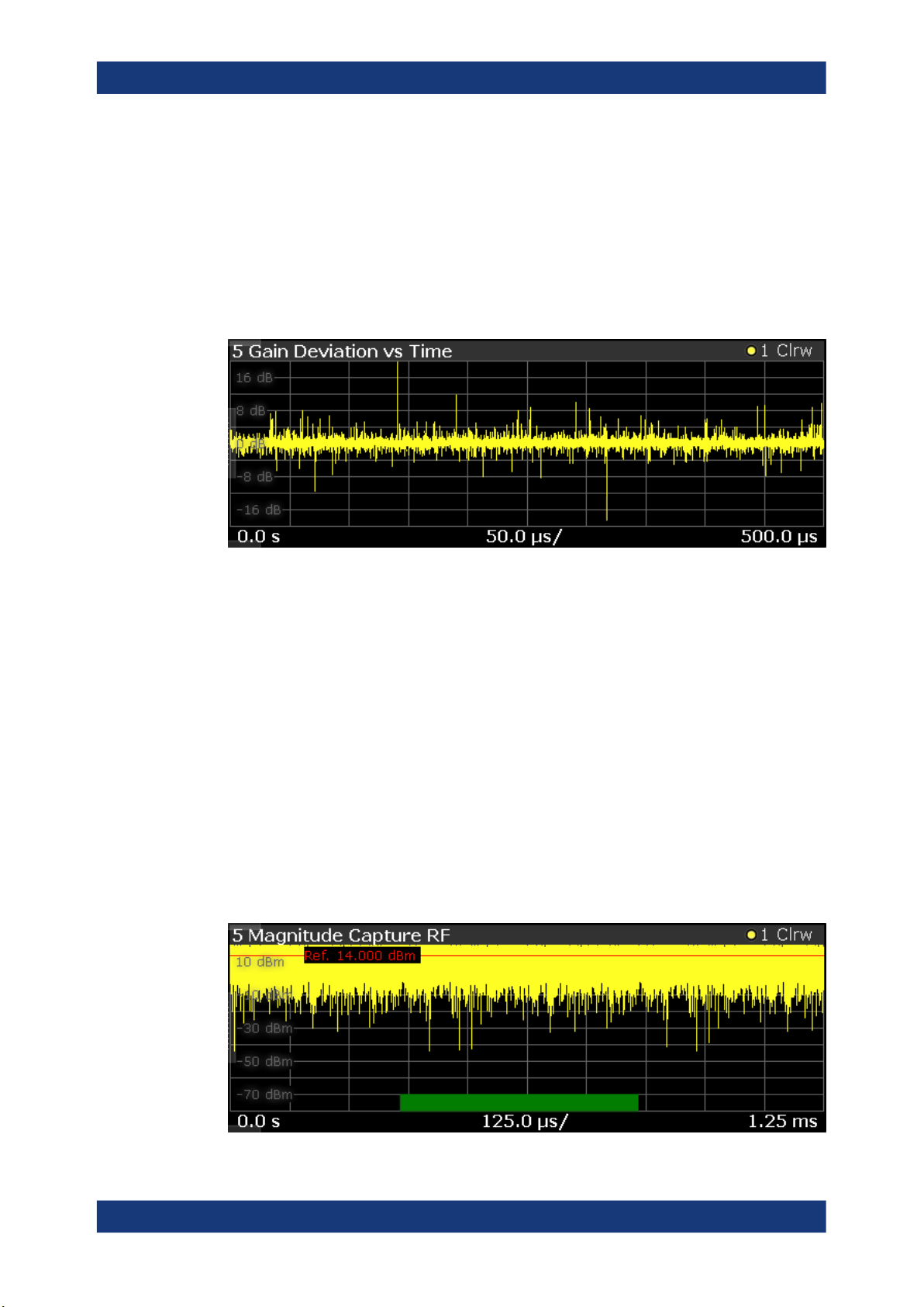
Gain Deviation vs Time

The "Gain Deviation vs Time" result display shows the deviation of each measured sig­nal sample from the average gain of the measured signal.

The x-axis shows the time in seconds. The y-axis shows the gain deviation in dB.
The displayed results are based on the synchronized measurement data (represented

by the green bar in the capture buffer).
Note that the result query and trace export only work for unencrypted reference signal

waveform files.

Remote command:
Selection: LAY:ADD? '1',LEFT,GDVT
Result query: TRACe<n>[:DATA]? on page 150

Magnitude Capture

The "Magnitude Capture" result display contains the raw data that has been recorded
and thus represents the characteristics of the DUT.

The capture buffer shows the signal level over time. The unit is either dBm.
The raw data is source for all further evaluations. You can also use the data in the cap-

ture buffer to identify the causes for possible unexpected results.
When you synchronize the reference signal and the measured signal, the synchronized

area is indicated by a horizontal green bar on the bottom of the diagram.
The current reference level is indicated by a red horizontal line.
The green bar at the bottom shows the current frame. In I/Q averaging mode, the aver-

age value is shown. In trace statistics mode, multiple values are possible. The currently
selected value is symbolized by a blue bar.

19User Manual 1178.9978.02 ─ 08

R&S®FSV3-K18

Measurements and result displays

Remote command:
Selection (RF): LAY:ADD? '1',LEFT,RFM
Result query: TRACe<n>[:DATA]? on page 150

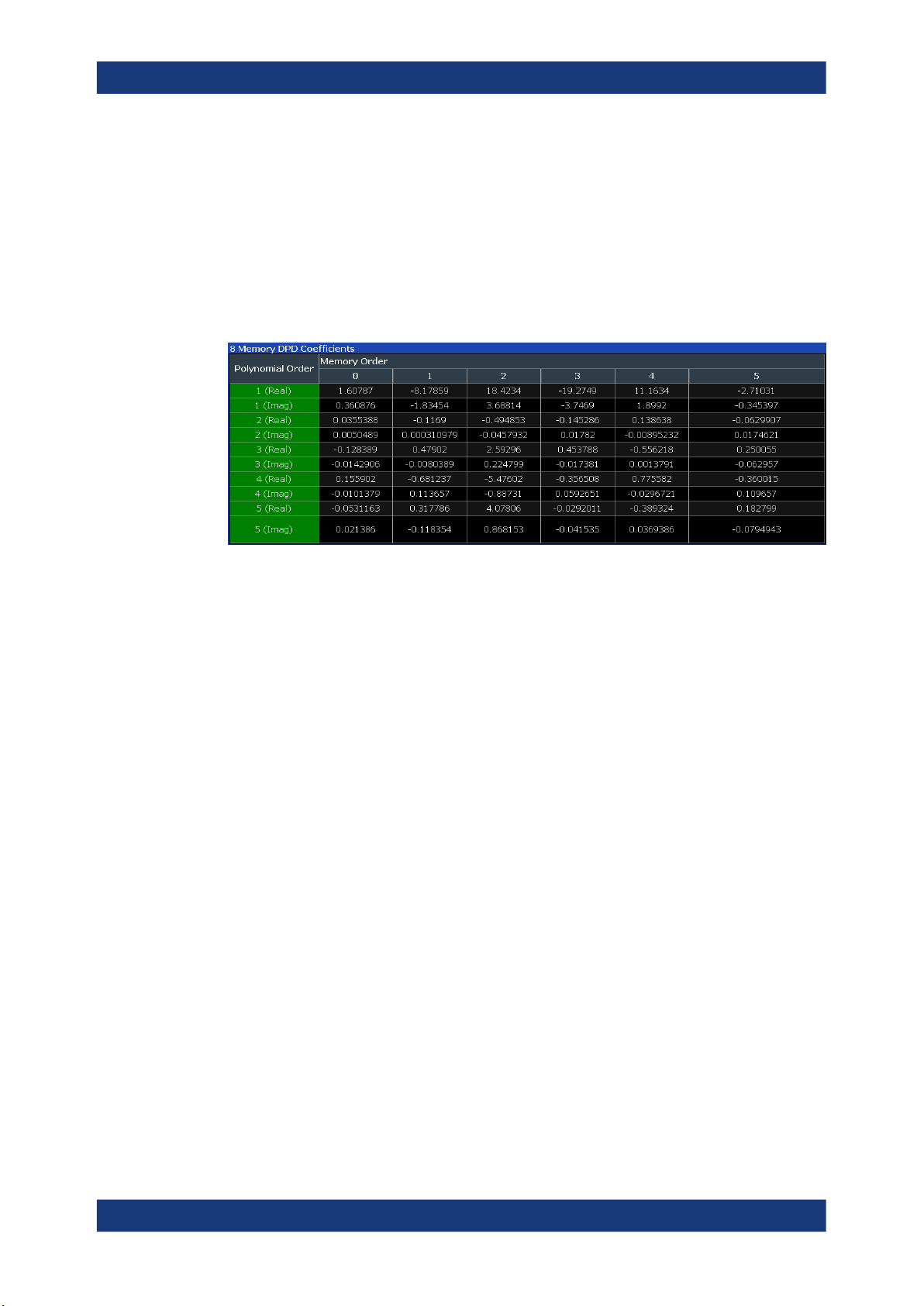
Memory DPD Coefficients

The "Memory DPD Coefficients" result table shows basically complex filter coefficients
for each polynomial degree. The two lines "1(Real)" and "1(Imag)" describe the com­plex impulse response for polynomial degree 1 (linear) of a filter from left to right. It is
only available with application R&S FSV/A-K18M installed.

Remote command:
Selection: LAY:ADD? '1',LEFT,MDPD
Result query: FETCh:MDPD:COEFficients? on page 309

Parameter Sweep

The "Parameter Sweep" result display is a result display that shows a result of the DUT
(for example the EVM) against two (custom) measurement parameters. The results of
this measurement are displayed in graphical and numerical form.

The parameter sweep is a good way, for example, to find the location of the ideal delay
time of the RF signal and the envelope signal if you are measuring an amplifier that
supports envelope tracking. You can also use the parameter sweep to determine the
characteristics and behavior of an amplifier over different frequencies and levels.

For more information about supported parameters and how to set them up see "Select-

ing the data to be evaluated during the parameter sweep" on page 108.

Parameter Sweep: Diagram ← Parameter Sweep

The parameter sweep diagram is a graphical representation of the parameter sweep
results. The results are either represented as a two-dimensional trace or as a three­dimensional trace, depending on whether you are performing a parameter sweep with
one or two parameters.

In a two-dimensional diagram, the y-axis always shows the result. The displayed result
depends on the result type you have selected. The information displayed on the x-axis
depends on the parameter you have selected for evaluation (for example the EVM over
a given frequency range). Values between measurement point are interpolated. Basi­cally, you can interpret the two-dimensional diagram as follows (example): "at a fre­quency of x Hz, the EVM has a value of y."

20User Manual 1178.9978.02 ─ 08

R&S®FSV3-K18

Measurements and result displays

In a three-dimensional diagram, the z-axis always shows the result. The information on
the other two axes is arbitrary and depends on the parameters you have selected for
evaluation. For a better readability, the result values in the three-dimensional diagram
are represented by a colored trace: low values have a blue color, while high values
have a red color. Values between measurement point are interpolated. Basically, you
can interpret the three-dimensional diagram as follows (example): "at a frequency of
x Hz and a level of y, the EVM has a value of z."

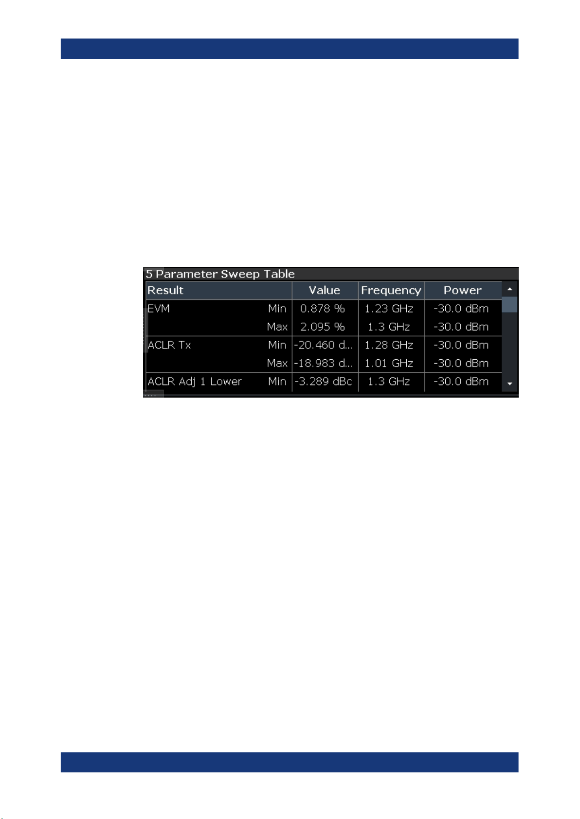
Parameter Sweep: Table ← Parameter Sweep

The parameter sweep table shows the minimum and maximum results for all available
result types in numerical form. For each result type, the location where the minimum
and maximum result has occurred is displayed.

Example:

A minimum EVM of 0.244 % and a maximum EVM of 0.246 % has been measured
(first and second row). The minimum EVM has been measured at a frequency of
30 MHz and an output power of 0 dBm. The maximum EVM has been measured at a
frequency of 10 MHz and an output power of 0 dBm.

The following result types are evaluated in the parameter sweep.

Result Description

EVM Error vector magnitude between synchronized reference and mea-

surement signal.

ACLR Power of the transmission channel.

ACLR Adj Upper / Lower Power of the adjacent channels (upper and lower).

ACLR Balanced (Adj, Alt1 and
Alt2)

RMS Power RMS signal power at the DUT output.

Gain Gain of the DUT.

Crest Factor Out Crest factor of the signal at the DUT output. The crest factor is the

Curve Width ("AM/AM", "AM/PM") Spread of the samples in the "AM/AM" (or "AM/PM") result display

Power Out Signal power at the DUT output.

Difference between the lower and upper adjacent channel power

ratio of the RMS and peak power.

compared to the ideal "AM/AM" (or "AM/PM") curve.

21User Manual 1178.9978.02 ─ 08

R&S®FSV3-K18

Measurements and result displays

Result Description

Compression Point (1 dB / 2 dB /
3 dB)

Bal ACLR Magnitude Shows the difference between the lower and upper adjacent channel

Input power where the gain deviates by 1 dB, 2 dB or 3 dB from a ref­erence gain (see "Configuring compression point calculation"
on page 103).

power.

Remote command:

Chapter 5.5.3.3, "Retrieving results of the parameter sweep table", on page 164

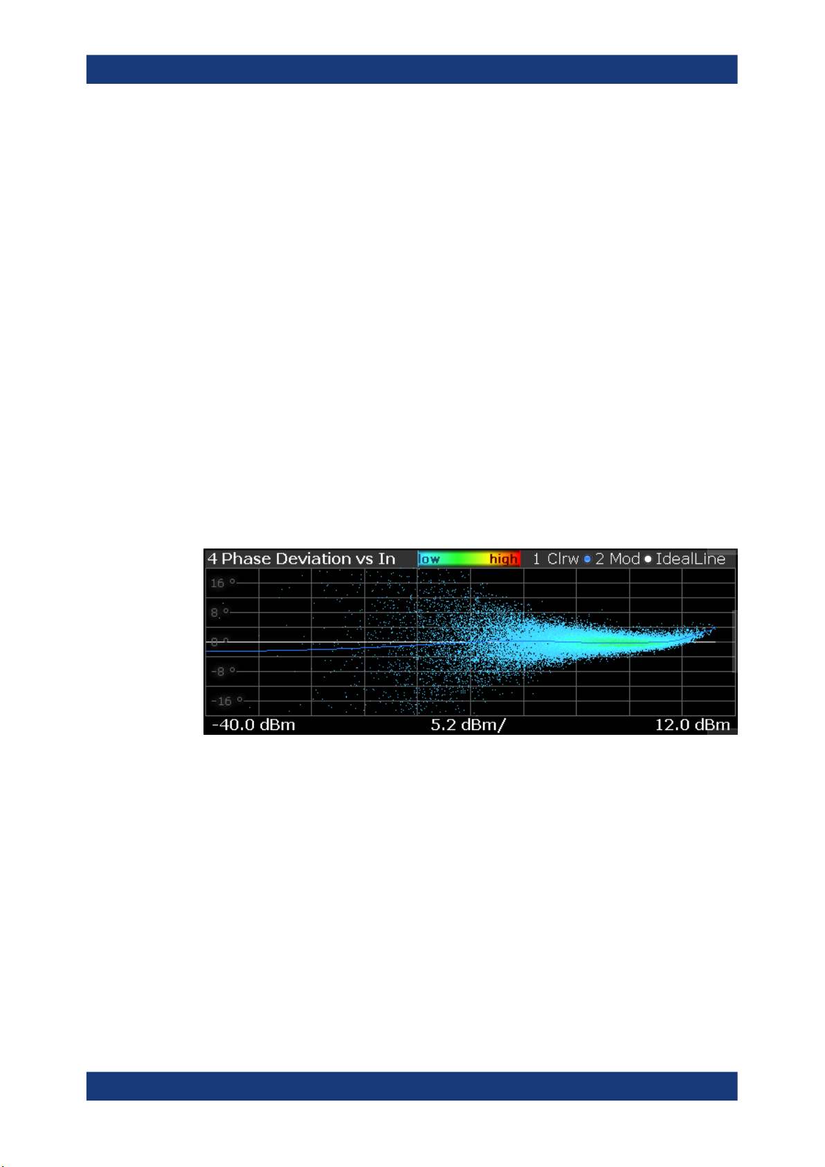
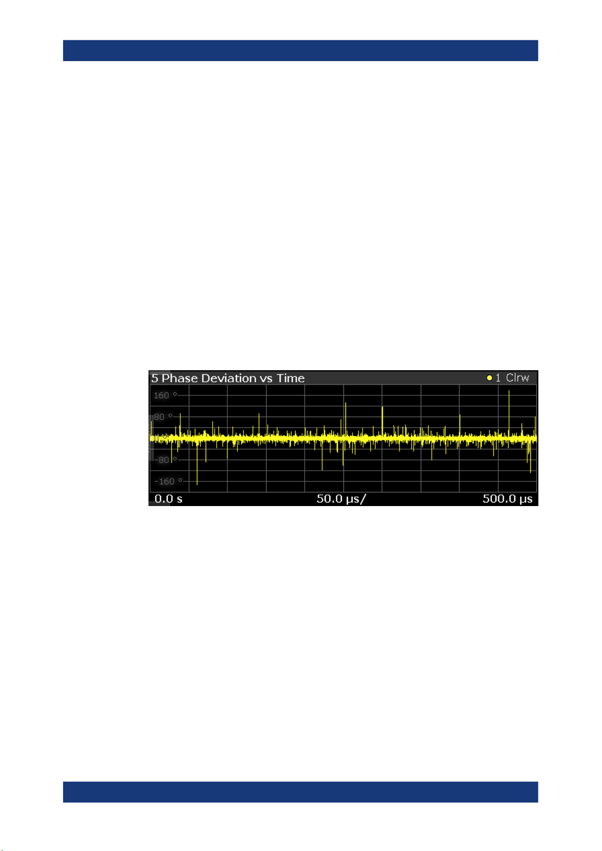
Phase Deviation vs Time

The "Phase Deviation vs Time" result display shows the phase deviation of the mea­sured signal compared to the reference signal over time.

The x-axis shows the time in seconds. The y-axis shows the phase deviation in
degree.

The displayed results are based on the synchronized measurement data (represented
by the green bar in the capture buffer).

Note that the result query and trace export only work for unencrypted reference signal
waveform files.

Remote command:
Selection: LAY:ADD? '1',LEFT,PDVT
Result query: TRACe<n>[:DATA]? on page 150

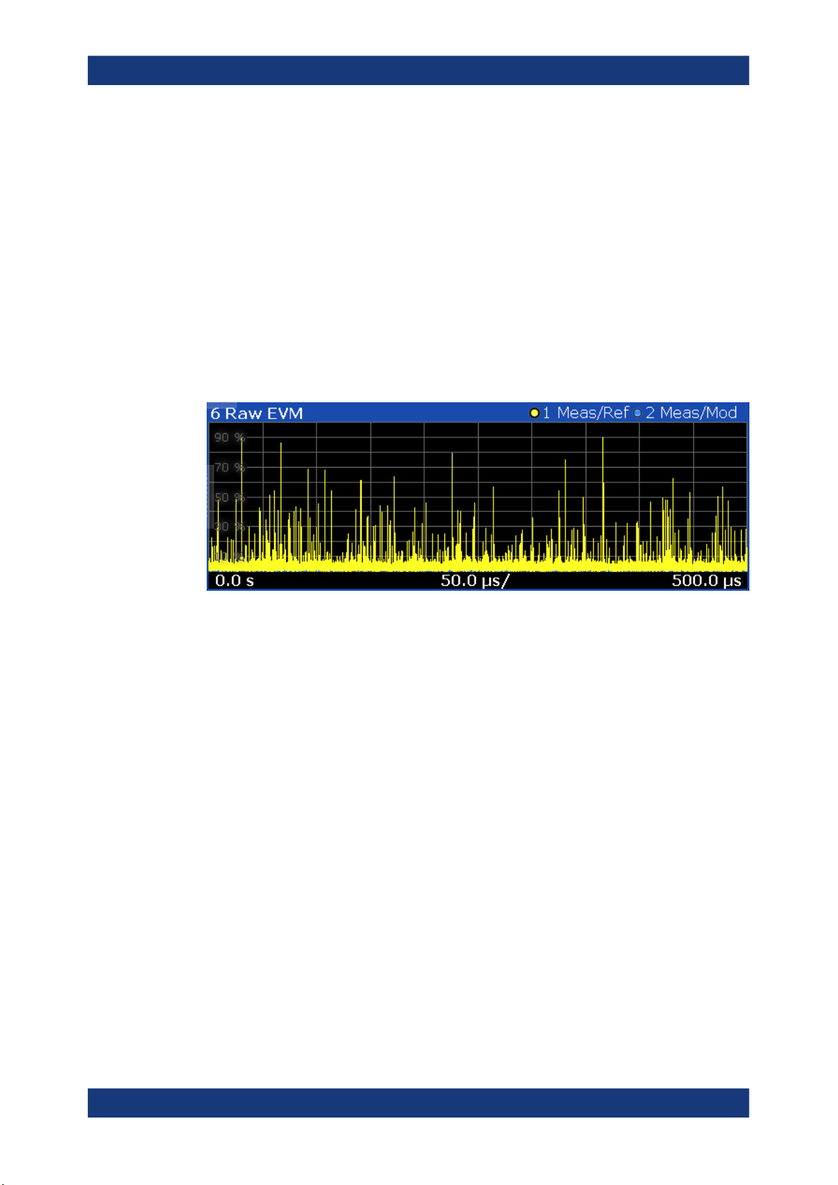
Raw EVM

The "Raw EVM" result display shows the error vector magnitude of the signal over
time.

The EVM is a measure of the modulation accuracy. It compares two signals and shows
the distance of the measured constellation points and the ideal constellation points.

You can compare the measured signal against the reference signal and against the
modeled signal.

●

Measured signal against reference signal
Trace 1 compares the measured signal and the reference signal.
To get useful results, the calculated linear gain is compensated to match both sig­nals.

22User Manual 1178.9978.02 ─ 08

R&S®FSV3-K18

Measurements and result displays

Depending on the DUT, noise and nonlinear effects may have been added to the
measurement signal. These effects are visualized by this trace.

●

Measured signal against modeled signal
Trace 2 compares the measured signal and the modeled signal.
The EVM between the measured and modeled signal indicates the quality of the
DUT modeling. If the model matches the DUT behavior, the modeling error is zero
(or is merely influenced by noise).
This result display shows changes in the model and its parameters and thus allows
you to optimize the modeling.
When system modeling has been turned off, this trace is not displayed.

Note that the raw EVM is calculated for each sample that has been recorded. Thus, the
raw EVM can differ from EVM values that are calculated according to a specific mobile
communication standard that apply special rules to calculate the EVM, for example
LTE.

Remote command:
Selection: LAY:ADD? '1',LEFT,REVM
Result query: TRACe<n>[:DATA]? on page 150

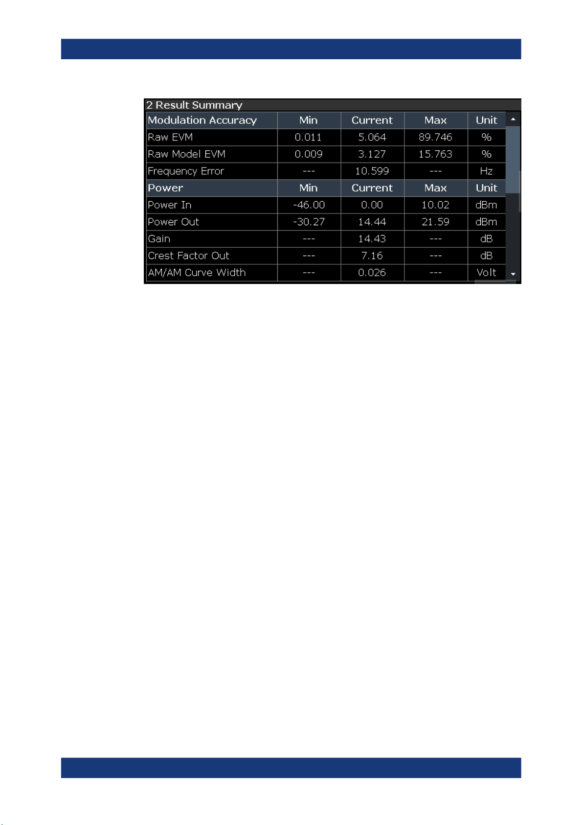
Numeric Result Summary

The "Result Summary" shows various measurement results in numerical form, com­bined in one table.

The table is split in two parts.

●

The first part shows the modulation accuracy

●

The second part shows the power characteristics of the RF signal

23User Manual 1178.9978.02 ─ 08

R&S®FSV3-K18

Measurements and result displays

For each result type, several values are displayed.

●

Current

Value measured during the last sweep.
For measurements that evaluate each captured sample, this value represents the
average value over all samples captured in the last sweep.

●

Min

For measurements that evaluate each captured sample, this value represents the
sample with lowest value captured in the last sweep.

●

Max

For measurements that evaluate each captured sample, this value represents the
sample with the highest value captured in the last sweep.

●

Unit

Unit of the result.

Results that evaluate each captured sample

●

"Raw EVM" and Raw Model EVM

●

Power In and Power Out

Note: When synchronization has failed or has been turned off, some results may be
unavailable.

Remote command:
Selecting the result display: LAY:ADD? '1',LEFT,RTAB
Querying results: see Chapter 5.5.3, "Retrieving numeric results", on page 152

24User Manual 1178.9978.02 ─ 08

R&S®FSV3-K18

Measurements and result displays

Results to check modulation accuracy ← Numeric Result Summary

Raw EVM Error vector magnitude between synchronized reference and measured sig-

nal.

FETCh:MACCuracy:REVM:CURRent[:RESult]? on page 156

Raw Model EVM Error vector magnitude between synchronized measured and model signal.

FETCh:MACCuracy:RMEV:CURRent[:RESult]? on page 157

Frequency Error Difference of the RF frequency of the reference signal compared to the mea-

sured signal.
Note that a frequency error is not available if the frequency error estimation is

switched off. See also Chapter 3.10, "Estimating and compensating signal

errors", on page 85.

FETCh:MACCuracy:FERRor:CURRent[:RESult]? on page 154

Sample Rate Error Sample rate difference between reference and measured signal.

Note that a sample rate error is not available if the sample rate error estima­tion is switched off. See also Chapter 3.10, "Estimating and compensating sig-

nal errors", on page 85.

FETCh:MACCuracy:SRERror:CURRent[:RESult]? on page 157

Magnitude Error Difference in magnitude between the reference signal and the measured sig-

nal.

FETCh:MACCuracy:MERRor:CURRent[:RESult]? on page 155

25User Manual 1178.9978.02 ─ 08

R&S®FSV3-K18

Measurements and result displays

Phase Error Phase difference between reference and measured signal.

FETCh:MACCuracy:PERRor:CURRent[:RESult]? on page 156

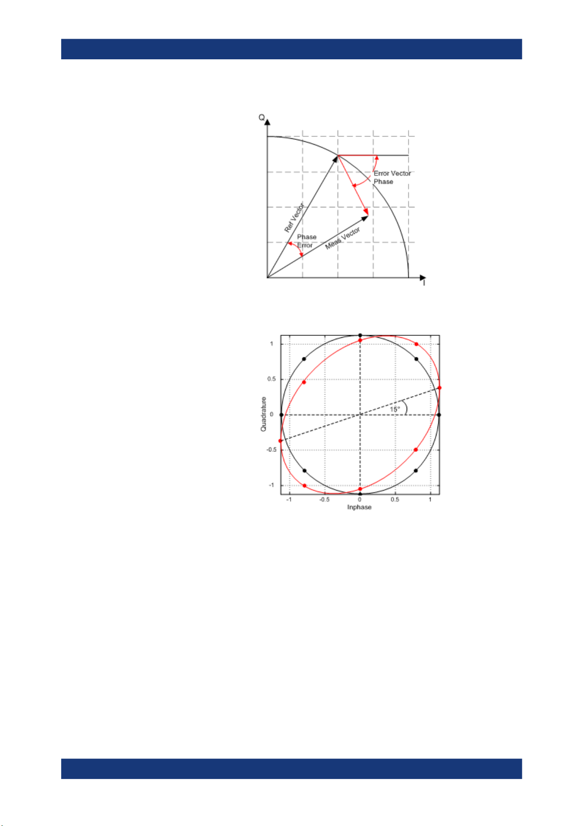
Quadrature Error Phase deviation of the 90° phase difference between the real (I) and imagi-

nary (Q) part of the signal.

Within an ideal transmitter, the I and Q signal parts are mixed with an angle of
90° by the I/Q output mixer. Due to hardware imperfections, the signal delay of
I and Q can be different and thus lead to an angle non-equal to 90°.

Note that quadrature rate error is not available if the I/Q Imbalance estimation
is switched off. See also Chapter 3.10, "Estimating and compensating signal

errors", on page 85.

FETCh:MACCuracy:QERRor:CURRent[:RESult]? on page 156

26User Manual 1178.9978.02 ─ 08

R&S®FSV3-K18

Measurements and result displays

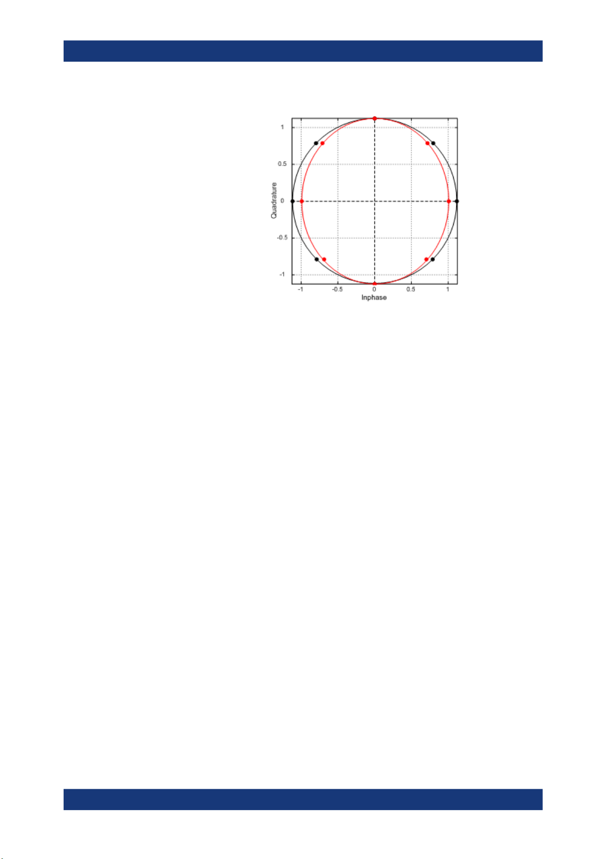
Gain Imbalance Gain difference between the real (I) and imaginary (Q) part of the signal.

This effect is typically generated by two separate amplifiers with a different
gain in the I and Q path of the analog baseband signal generation.

Note that gain imbalance is not available if the I/Q Imbalance estimation is
switched off. See also Chapter 3.10, "Estimating and compensating signal

errors", on page 85.

FETCh:MACCuracy:GIMBalance:CURRent[:RESult]? on page 154

I/Q Imbalance Combination of Quadrature error and Gain imbalance.

The I/Q imbalance parameter is a representation of the combination of Quad­rature error and gain imbalance.

Note that I/Q imbalance is not available if the I/Q imbalance estimation is
switched off. See also Chapter 3.10, "Estimating and compensating signal

errors", on page 85.

FETCh:MACCuracy:IQIMbalance:CURRent[:RESult]? on page 155

27User Manual 1178.9978.02 ─ 08

R&S®FSV3-K18

Measurements and result displays

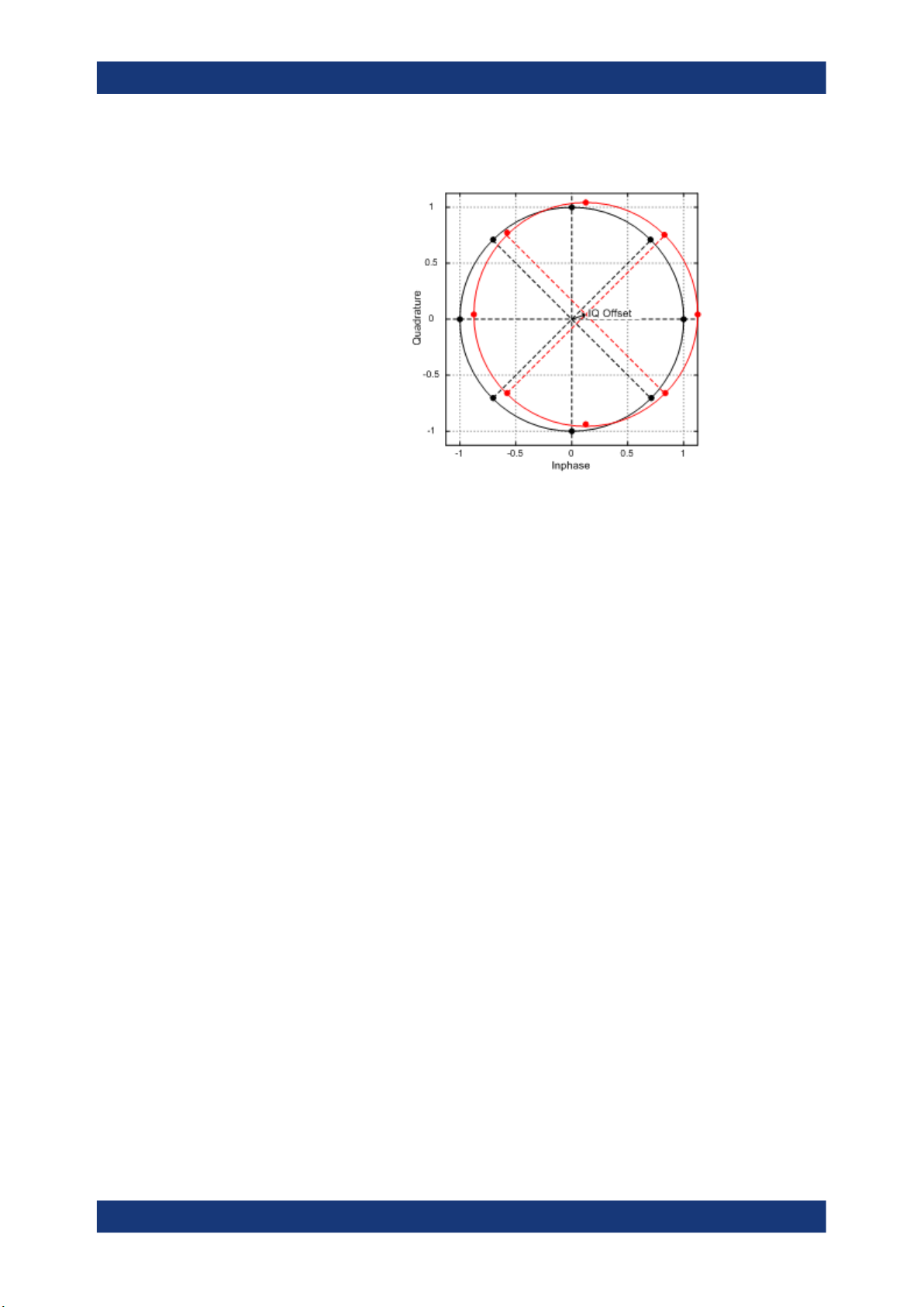
I/Q Offset Shift of the measured signal compared to the ideal I/Q constellation in the I/Q

plane.

Note that I/Q offset is not available if the I/Q Offset estimation is switched off.
See also Chapter 3.10, "Estimating and compensating signal errors",
on page 85.

FETCh:MACCuracy:IQOFfset:CURRent[:RESult]? on page 155

Amplitude Droop Amplitude droop is a measure of the change in magnitude of the signal over

the frame (reference signal) being measured in dB.
Note that amplitude droop is not available if the amplitude droop estimation is

switched off. See also Chapter 3.10, "Estimating and compensating signal

errors", on page 85.

Results to check power characteristics ← Numeric Result Summary

Power In Signal power at the DUT input when reference signal is active. The signal

generator level may change during direct DPD, but this result summary value
will always refer to the reference signal – not the DPD signal.

FETCh:POWer:INPut:CURRent[:RESult]? on page 160

Power In (Sensor) Signal power at the input power sensor.

FETCh:POWer:SENSor:IN:CURRent[:RESult]? on page 163

Power Out Signal power at the DUT output.

Power Out (Sensor) Signal power at the output power sensor.

It is the RMS power of:

●

The currently selected frame, if R&S FSV/A-K18 has successfully
synchronized.

●

The current capture buffer, if R&S FSV/A-K18 has not synchronized.

FETCh:POWer:OUTPut:CURRent[:RESult]? on page 160

FETCh:POWer:SENSor:OUT:CURRent[:RESult]? on page 164

28User Manual 1178.9978.02 ─ 08

R&S®FSV3-K18

Measurements and result displays

Gain Average gain calculated over all samples of the "Gain Compression" trace.

noise in

output signal

gain

Note that gain is not necessarily equal to the ratio "Power Out" / "Power In".
Gain only describes the ratio of the correlated signal in "Power Out" to "Power
In".

Gain is always referenced to the reference signal power, i.e. when DPD
changes the generator level, the gain is still referenced to the input power of
the reference signal - not the DPD signal.

Example: If the output signal contains the same amount of noise as the corre­lated signal (e.g. signal is 0 dBm and noise power is also 0 dBm), "Power Out"
will show the sum (3 dBm). However, assuming an input signal power of

-10 dBm, gain will only show 10 dB, not 13 dB.

FETCh:POWer:GAIN:CURRent[:RESult]? on page 159

total output

signal

correlated

output signal

input signal

Crest Factor In Crest factor of the signal at the DUT input. The crest factor is the ratio of the

RMS and peak power.

FETCh:POWer:CFACtor:IN:CURRent[:RESult]? on page 159

Crest Factor Out Crest factor of the signal at the DUT output. The crest factor is the ratio of the

RMS and peak power.

FETCh:POWer:CFACtor:OUT:CURRent[:RESult]? on page 159

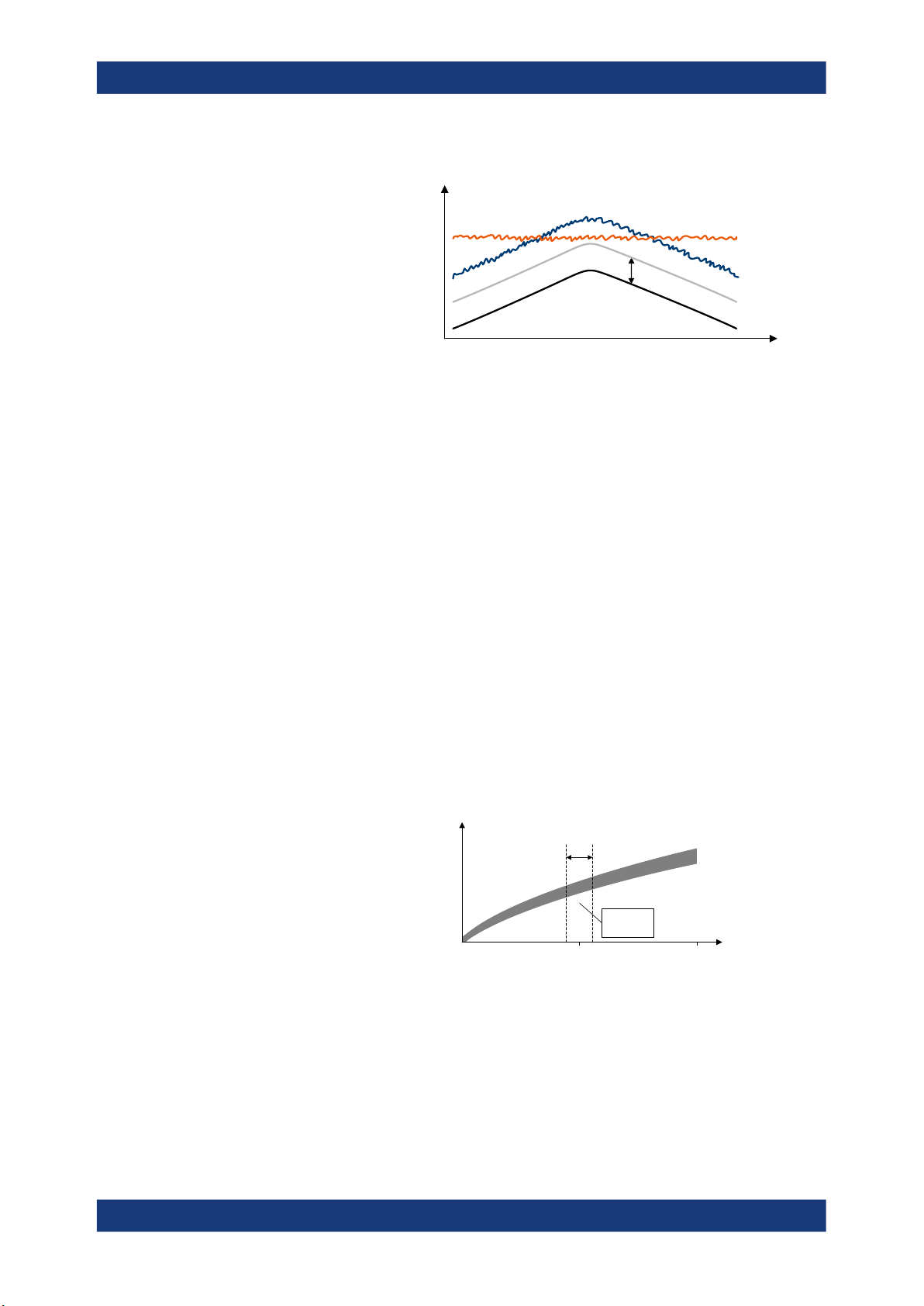
AM/AM Curve Width Vertical spread of the samples in the "AM/AM" result display.

The "AM/AM" curve width shows the standard deviation of the output voltage
or the output phase deviation within a +/- 1% range around the mean ampli­tude in volt.

Output

amplitude

+/- 1%

σ of output

amplitude

in this range

10,5

Input amplitude

linear normalized

FETCh:AMAM:CWIDth:CURRent[:RESult]? on page 158

29User Manual 1178.9978.02 ─ 08

R&S®FSV3-K18

Measurements and result displays

AM/PM Curve Width Vertical spread of the samples in the "AM/PM" result display.

The "AM/PM" curve width shows the standard deviation of the output voltage
or the output phase deviation within a +/- 1% range around the mean ampli­tude in volt.

Output

amplitude

+/- 1%

σ of output

amplitude

in this range

FETCh:AMPM:CWIDth:CURRent[:RESult]? on page 158

10,5

Input amplitude

linear normalized

Compression Point (1 dB / 2
dB / 3 dB)

Input power where the gain deviates by 1 dB, 2 dB or 3 dB from a reference
gain (see "Configuring compression point calculation" on page 103).

In the graphical result, the compression points are indicated by horizontal red
lines.

FETCh:POWer:P1DB:CURRent[:RESult]? on page 160

FETCh:POWer:P2DB:CURRent[:RESult]? on page 161

FETCh:POWer:P3DB:CURRent[:RESult]? on page 161

Output Compression Point
(1 dB / 2 dB / 3 dB)

Output power where the gain deviates by 1 dB, 2 dB or 3 dB from a reference
gain.

Uses identical operating points as "Compression Point (1 dB / 2 dB / 3 dB)",
but is identified by output power at compression point rather than input power.

FETCh:POWer:P1DB:OUT:CURRent[:RESult]? on page 162

FETCh:POWer:P2DB:OUT:CURRent[:RESult]? on page 162

FETCh:POWer:P3DB:OUT:CURRent[:RESult]? on page 163

Occupied Bandwidth Occupied bandwidth calculated for the defined evaluation range.

Spectrum FFT

The "Spectrum FFT" result display shows the frequency spectrum of the signal.
The spectrum FFT result shows the signal level in the spectrum around the center fre-

quency. The unit is dBm.
You can display the spectrum of the measured signal and the reference signal. In the

best case, the measured signal has the same shape as the reference signal.

30User Manual 1178.9978.02 ─ 08

R&S®FSV3-K18

Measurements and result displays

Remote command:
Selection (RF): LAY:ADD? '1',LEFT,RFS
Result query: TRACe<n>[:DATA]? on page 150

Time Domain

The "Time Domain" result display shows the signal characteristics over time.
It is similar to the "Power vs Time" and "Magnitude Capture" result displays in that it

shows the signal characteristics over time. However, it deliberately shows only a very
short period of the signal. You can thus use it to compare various aspects of the signal,
especially the timing of the displayed signals, in a single result display.

●

Measured signal
Trace 1 shows the characteristics of the measured signal over time. The data
should be the same as the results shown in the "Magnitude Capture" RF result dis­play.
In the best case, the measured signal is the same as the reference signal.

●

Modeled signal
Trace 2 shows the characteristics of the modeled signal. When system modeling
has been turned off, this trace is not displayed.
If the model matches the behavior of the DUT, the characteristics of the signal are
the same as those of the measured signal (minus the noise).

●

Reference signal
Trace 3 shows the characteristics of the reference signal. The reference signal
present at the DUT input represents the ideal signal.

Remote command:
Selection: LAY:ADD? '1',LEFT,TDOM
Result query: TRACe<n>[:DATA]? on page 150

Scale of the x-axis (display settings for the time domain) ← Time Domain

The scale of the x-axis depends on your configuration in the "Display Settings" dialog
box.

The logic is as follows:

●

When you select automatic scaling (➙ "Position: Auto") and synchronization has
failed, the application searches for the peak level in the capture buffer and shows
the signal around the peak for the "Duration" that has been defined.

●

When you select automatic scaling (➙ "Position: Auto") and synchronization is OK,
the application searches for the peak level in the synchronized area of the capture

31User Manual 1178.9978.02 ─ 08

R&S®FSV3-K18

Measurements and result displays

buffer and shows the signal around the peak for the "Duration" that has been
defined.

●

When you select manual scaling (➙ "Position: Manual") and synchronization has
failed, the x-axis starts at an "Offset" relative to the first sample in the capture buf­fer. The end of the x-axis depends on the "Duration" you have defined.

●

When you select manual scaling (➙ "Position: Manual") and synchronization is OK,
the x-axis starts at an "Offset" relative to the first sample in the synchronized area
of the capture buffer. The end of the x-axis depends on the "Duration" you have
defined.

Note: The "Display Settings" for the time domain are only available after you have
selected the "Specifics for: Time Domain" item from the corresponding dropdown menu
at the bottom of the dialog box.

Scale of the y-axis (display settings for the time domain) ← Time Domain

The scale of the y-axis also depends on your configuration.
The signal characteristics displayed in the time domain result display all have a differ-

ent unit. Therefore, the application provides a feature that normalizes all results to 1
(see "Configuring the time domain result display" on page 123). Normalization makes it
easier to compare the timing between the traces. By default, normalization is on. Note
that you can normalize each "Time Domain" window individually.

Unnormalized results are displayed in their respective unit.

Statistics Table

The results for the statistics table are available only after the statistics mode has been
activated using [SENSe:]SWEep:STATistics[:STATe] on page 280. If statistics
mode is switched off, the statistics table stays empty.

Each value in the statistics table has different rows describing a single frame: Average,
Std. Dev, Maximum and Minimum. This is similar to the Numeric Result Summary.

The different color codes represent different result values:

●

Blue

Result of the current result range. The selected values are updated when the user
sweeps through the result range selection.

●

Green

In I/Q averaging mode, the values in the green area are identical to the ones in the
black background area.
In trace statistics mode, the green area refers to all frames of the current capture
buffer, whereas the black area refers to all measured frames (including previous

32User Manual 1178.9978.02 ─ 08

R&S®FSV3-K18

Measurements and result displays

capture buffers). Statistics is always done over sweep “Count” frames and then is
being reset, unless the "Continuous Statistics" switch is activated. In this case,
infinite statistics is executed.

●

Black / No selection

Statistical results that can also be based on result ranges that were captured in
previous measurement sweeps.

Remote command:
Adding statistics table: LAY:ADD? '1',LEFT,STAB
Querying results: Chapter 5.5.3.4, "Retrieving results of the statistics table",
on page 175
Configuring statistics table: Chapter 5.7.4, "Configuring the statistics table",
on page 344
Navigating through results ranges found in a capture: CONFigure:RESult:RANGe[:

SELected] on page 281

33User Manual 1178.9978.02 ─ 08

R&S®FSV3-K18

3 Configuration

Configuration

Configuration overview

● Configuration overview............................................................................................34

● Performing measurements......................................................................................36

● Designing a reference signal...................................................................................37

● Configuring inputs and outputs............................................................................... 49

● Triggering measurements....................................................................................... 75

● Configuring the data capture...................................................................................75

● Sweep configuration................................................................................................78

● Synchronizing measurement data...........................................................................80

● Evaluating measurement data................................................................................ 83

● Estimating and compensating signal errors............................................................ 85

● Equalizer................................................................................................................. 86

● Applying system models......................................................................................... 87

● Applying digital predistortion................................................................................... 90

● Detailed MSE........................................................................................................ 101

● Configuring power measurements........................................................................ 103

● Configuring adjacent channel leakage error (ACLR) measurements................... 104

● Configuring the parameter sweep.........................................................................106

● Configuring power servoing...................................................................................110

3.1 Configuration overview

Throughout the measurement channel configuration, an overview of the most important
currently defined settings is provided in the "Overview". The "Overview" is displayed
when you select the "Overview" icon, which is available at the bottom of all softkey
menus.

In addition to the main measurement settings, the "Overview" provides quick access to
the main settings dialog boxes. The individual configuration steps are displayed in the
order of the data flow. Thus, you can easily configure an entire measurement channel

34User Manual 1178.9978.02 ─ 08

R&S®FSV3-K18

Configuration

Configuration overview

from input over processing to output and analysis by stepping through the dialog boxes
as indicated in the "Overview".

In particular, the "Overview" provides quick access to the following configuration dialog
boxes (listed in the recommended order of processing):

1. Reference Signal

See Chapter 3.3, "Designing a reference signal", on page 37.

2. Input and output

See Chapter 3.4, "Configuring inputs and outputs", on page 49.

3. Trigger

See Chapter 3.5, "Triggering measurements", on page 75.

4. Data Acquisition

See Chapter 3.6, "Configuring the data capture", on page 75.

5. Synchronization, error estimation and compensation

See Chapter 3.8, "Synchronizing measurement data", on page 80.
See Chapter 3.10, "Estimating and compensating signal errors", on page 85.

6. Measurement

Modeling: see Chapter 3.12, "Applying system models", on page 87.
DPD: see Chapter 3.13, "Applying digital predistortion", on page 90.

7. Result configuration

See Chapter 4, "Analysis", on page 112.

8. Display configuration

See Chapter 2, "Measurements and result displays", on page 10.

To configure settings

► Select any button in the "Overview" to open the corresponding dialog box.

Select a setting in the channel bar (at the top of the measurement channel tab) to
change a specific setting.

Preset Channel

Select the "Preset Channel" button in the lower left-hand corner of the "Overview" to
restore all measurement settings in the current channel to their default values.

Note: Do not confuse the "Preset Channel" button with the [Preset] key, which restores
the entire instrument to its default values and thus closes all channels on the
R&S FSV/A (except for the default channel)!

Remote command:

SYSTem:PRESet:CHANnel[:EXEC] on page 138

Specific Settings for

The channel can contain several windows for different results. Thus, the settings indi­cated in the "Overview" and configured in the dialog boxes vary depending on the
selected window.

35User Manual 1178.9978.02 ─ 08

R&S®FSV3-K18

3.2 Performing measurements

Configuration

Performing measurements

Select an active window from the "Specific Settings for" selection list that is displayed
in the "Overview" and in all window-specific configuration dialog boxes.

The "Overview" and dialog boxes are updated to indicate the settings for the selected
window.

Access: [SWEEP]

The following features control the measurement. They are available in the "Sweep"
menu.

The remote commands required to control the measurement are described in Chap-

ter 5.5.1, "Performing measurements", on page 146.

Continuous Sweep / Run Cont......................................................................................36

Single Sweep / Run Single............................................................................................36

Continue Single Sweep.................................................................................................37

Continuous Sweep / Run Cont

After triggering, starts the measurement and repeats it continuously until stopped. This
is the default setting.

While the measurement is running, the "Continuous Sweep" softkey and the [RUN
CONT] key are highlighted. The running measurement can be aborted by selecting the
highlighted softkey or key again. The results are not deleted until a new measurement
is started.

Note: Sequencer. If the Sequencer is active, the "Continuous Sweep" softkey only con­trols the sweep mode for the currently selected channel. However, the sweep mode
only takes effect the next time the Sequencer activates that channel, and only for a
channel-defined sequence. In this case, a channel in continuous sweep mode is swept
repeatedly.
Furthermore, the [RUN CONT] key controls the Sequencer, not individual sweeps.
[RUN CONT] starts the Sequencer in continuous mode.

For details on the Sequencer, see the R&S FSV/A User Manual.
Remote command:

INITiate<n>:CONTinuous on page 146

Single Sweep / Run Single

After triggering, starts the number of sweeps set in "Sweep Count". The measurement
stops after the defined number of sweeps has been performed.

While the measurement is running, the "Single Sweep" softkey and the [RUN SINGLE]
key are highlighted. The running measurement can be aborted by selecting the high­lighted softkey or key again.

Note: Sequencer. If the Sequencer is active, the "Single Sweep" softkey only controls
the sweep mode for the currently selected channel. However, the sweep mode only
takes effect the next time the Sequencer activates that channel, and only for a chan-

36User Manual 1178.9978.02 ─ 08

R&S®FSV3-K18

Configuration

Designing a reference signal

nel-defined sequence. In this case, the Sequencer sweeps a channel in single sweep
mode only once.
Furthermore, the [RUN SINGLE] key controls the Sequencer, not individual sweeps.
[RUN SINGLE] starts the Sequencer in single mode.

If the Sequencer is off, only the evaluation for the currently displayed channel is upda­ted.

For details on the Sequencer, see the R&S FSV/A User Manual.
Remote command:

INITiate<n>[:IMMediate] on page 147

Continue Single Sweep

While the measurement is running, the "Continue Single Sweep" softkey and the [RUN
SINGLE] key are highlighted. The running measurement can be aborted by selecting
the highlighted softkey or key again.

Remote command:

INITiate<n>:CONMeas on page 146

3.3 Designing a reference signal

Access (source: generator): "Overview" > "Reference Signal" > "Current Generator

Waveform"

Access (source: waveform file): "Overview" > "Reference Signal" > "Custom Wave­form File"

Access (source: Amplifier application): "Overview" > "Reference Signal" > "Generate
Own Signal"

Many of the results available in the application require a reference signal that
describes the characteristics of the signal you feed into the amplifier.

The reference signal describes the characteristics of the signal that you feed into the
amplifier and whose amplified version is measured by the application. You can define
any signal you want as a reference signal.

The application provides several methods to design a reference signal:

●

Designing the signal on a generator
(Having a Rohde & Schwarz generator is mandatory for this method.)

●

Designing the signal in a waveform file

●

Designing the signal in the amplifier application
(Having a Rohde & Schwarz generator is mandatory for this method.)

For a list of supported signal generators, refer to the datasheet of the amplifier applica­tion.

The remote commands required to configure the reference signal are described in

Chapter 5.6.1, "Designing a reference signal", on page 230.

37User Manual 1178.9978.02 ─ 08

R&S®FSV3-K18

Configuration

Designing a reference signal

Reference signal information........................................................................................ 38

Using multi-segment waveform files............................................................................. 39

Transferring the reference signal.................................................................................. 39

Designing a reference signal on a signal generator......................................................40

Designing a reference signal in a waveform file............................................................41

Designing a reference signal within the R&S FSV3-K18.............................................. 43

└ Signal Bandwidth............................................................................................ 44

└ Pulse Duty Cycle.............................................................................................45

└ Signal Length..................................................................................................45

└ Ramp Length.................................................................................................. 45

└ Target Crest Factor......................................................................................... 45

└ Waveform File Name...................................................................................... 45

└ Notch Width.................................................................................................... 45

└ Notch Position.................................................................................................46

Crest Factor Reduction (Generator Option K548).........................................................46

└ Crest Factor Reduction State..........................................................................47

└ EVM Ref. Signal..............................................................................................47

└ Crest Factor Delta...........................................................................................47

└ Current Crest Factor....................................................................................... 48

└ Max Iterations................................................................................................. 48

└ Filter Mode......................................................................................................48

└ Signal Bandwidth............................................................................................ 48

└ Channel Spacing.............................................................................................48

└ Read CFR from Generator, Load....................................................................48

└ Passband Frequency......................................................................................49

└ Stopband Frequency.......................................................................................49

└ Maximum Filter Order..................................................................................... 49

Reference signal information

Each tab of the "Reference Signal" dialog box contains some basic information about
the reference signal currently in use.

The information is only displayed when a reference signal has been successfully loa­ded. When you load a different waveform, the reference signal information is updated
accordingly.

●

Waveform file
Name and path of the waveform file currently in use.

●

Sample rate
The sample rate in the header of the currently used reference signal waveform file
in Hz.

●

Number of samples
Length of the currently used reference signal waveform file in samples.

●

Crest Factor (File)
Crest factor of the whole file currently in use. The crest factor of waveform files is
read from their header. The crest factor of iq.tar files is calculated.

●

Bandwidth (OBW)

38User Manual 1178.9978.02 ─ 08

R&S®FSV3-K18

Configuration

Designing a reference signal

The occupied bandwidth of the reference signal currently in use. A calculated
bandwidth that contains 99% of signal power is displayed.

Remote command:
File path: CONFigure:REFSignal:SINFo:FPATh? on page 237
Sample rate: CONFigure:REFSignal:SINFo:SRATe? on page 238
Sample length: CONFigure:REFSignal:SINFo:SLENgth? on page 238
Crest Factor: CONFigure:REFSignal:SINFo:CFACtor? on page 238
OBW: CONFigure:REFSignal:SINFo:OBW? on page 239

Using multi-segment waveform files

Modern chip technologies implement several communication standards within one chip
and thus increase the requirements in spatial design and test systems. To fulfill the
requirements in the test systems, and to enable a rapid change between different
waveforms containing different test signals, the R&S SMW provides the functionality to
generate multi-segment waveform files. Multi-segment waveform files are files that
contain several different waveforms.

(For more information about creating and using multi-segment waveform files (includ­ing examples) refer to the documentation of the R&S SMW.)

When you are testing amplifiers with the amplifier measurement application, you can
use a multi-segment waveform file to create the reference signal. If you use one of
these files, you have to select the segment that you want to use as a reference signal
in the corresponding input field.

Note that the content of the segment you are using for the reference signal must match
the content of the segment used by the ARB of the signal generator. You can select the
segment for the used by the generator in the generator setup.

Remote command:

CONFigure:REFSignal:SEGMent on page 237

Transferring the reference signal

Both the signal generator and analyzer used in the test setup need to know the charac­teristics of the reference signal.

●

The signal generator needs that information to generate the signal.

●

The analyzer needs that information for the evaluation of the results.

This is why you have to transfer the signal information to both instruments. The trans­mission is done through a LAN connection that you have to establish when setting up
the measurement. For more information on that see Chapter 3.4.7, "Controlling a sig-

nal generator", on page 61.

●

When you design the reference signal on the signal generator, transfer the signal
information from the generator to the analyzer with the ➙"Read and Load Current
Signal from R&S SMW" button.
You can either design a reference signal with one of the available firmware options
(for example an LTE signal with the R&S SMW-K55) or design a signal in a custom
waveform file. Note that the R&S FSV3-K18 does not support all firmware options
of the signal generator.

●

When you load the reference signal from a waveform file or design the signal within
the R&S FSV3-K18, transfer the signal information from the analyzer to the gener­ator. Depending on the signal source, you can do this either with the "Load and

39User Manual 1178.9978.02 ─ 08

R&S®FSV3-K18

Configuration

Designing a reference signal

Export Selected Waveform File to Generator" or the "Generate and Load Signal
and Export it to Generator" buttons.

When you send the signal information to the generator, the application automatically
configures the generator accordingly.

Transmission state

The LED displayed with the transmission button shows the state of the reference signal
transmission.

The LED is either gray, green or red:

●

Grey LED
Transmission state unknown (for example when you have not yet started the trans­mission).

●

Green LED
Transmission has been successful.

●

Red LED
Transmission has not been successful.
Make sure that the generator control state is on.
Check if the generator IP address / computer name are correct and if the connec­tion has been established.

Designing a reference signal on a signal generator

One way to design a reference signal is to design the signal on the signal generator
itself.

You can design any signal you like, as long as it is storable as an arbitrary waveform
(ARB) file. When you are done, you have to transfer the signal information from the
signal generator to the signal analyzer with the "Read from Generator, Load" button.

The "Force ARB Mode" switch forces the signal generator to use its ARB mode (arbi­trary waveform) rather than its real-time mode, whenever possible. As a result, switch­ing between DPD on and off state is significantly faster. When the "Force ARB Mode"
function is used, the peak power of the generator is read out and used within the proc­ess but as a result of this function the RMS power of the generator is modified. Also
the waveform header of the file is recalculated to make sure that the peak input level
stays constant or lower than the gain expansion during DPD calculation.

The parameters of the currently active reference signal are described in "Reference

signal information" on page 38.

The "Open Generator Control" button provides functionality to change the generator
settings as described in Chapter 3.4.7, "Controlling a signal generator", on page 61.

40User Manual 1178.9978.02 ─ 08

R&S®FSV3-K18

Configuration

Designing a reference signal

Most of the options available for the connected generator are supported by the auto­matic signal import functionality of the R&S FSV3-K18. If the signal import was not suc­cessful (indicated by a red LED), you have to transfer the reference signal in another
way (for example with a memory stick).

For a comprehensive description of all features available on the signal generator and
information on how to generate signals, refer to the documentation of the signal gener­ator.

Remote command:
See signal generator documentation.

CONFigure:REFSignal:CGW:AMODe[:STATe] on page 231
CONFigure:REFSignal:CGW:READ on page 231
CONFigure:REFSignal:CGW:LEDState? on page 231

Designing a reference signal in a waveform file

One way to design a reference signal is to define its characteristics in a waveform file
(*.wv or *.iq.tar).

You can create a waveform file, for example:

●

With the R&S®WinIQSIM2 software package

●

By exporting a signal designed on the signal generator

Basically, this file contains the characteristics of the reference signal. The generator
then generates the reference signal based on the information in the file.

There are two ways to generate the reference signal through a custom waveform file.

●

The generator is connected to the R&S FSV/A in a LAN, and can be recognized by
the R&S FSV3-K18 (Rohde & Schwarz generators only, for example the
R&S SMW)

41User Manual 1178.9978.02 ─ 08

R&S®FSV3-K18

Configuration

Designing a reference signal

In that case, you can simply transfer the reference signal information to the genera­tor with the features integrated into the R&S FSV3-K18. The generator then gener­ates the corresponding signal with the appropriate signal level, and the R&S FSV3­K18 is able to compare the measured signal to the ideal reference signal.

●

The generator is not connected to the R&S FSV/A
In that case, you have to load the reference signal information onto the generator
manually and turn off the "Export to Generator" function. Because no exchange of
information is possible between generator and analyzer, it is required to specify the
input level of the signal in the "DUT Peak Input Power" input field.

The parameters of the currently active reference signal are described in "Reference

signal information" on page 38.

The "Open Generator Control" button provides functionality to change the generator
settings as described in Chapter 3.4.7, "Controlling a signal generator", on page 61.

For a comprehensive description of all features available on the signal generator and
information on how to generate and export signals to a file, refer to the documentation
of the signal generator.

To transfer a waveform file from the analyzer to the generator and process it with the
ARB generator of the R&S SMW, for example, proceed as follows:

▶ In the "Custom Waveform" tab, select a file via the "Load, Play on Generator" button.
▶ Transfer the file to the generator with the "Select" button.

If a waveform is only used as a reference without transferring it to the signal generator,
make sure that the generator control state "Off" is selected in the generator setup dia­log.

Remote command:
Select file: CONFigure:REFSignal:CWF:FPATh on page 233
Transfer file: CONFigure:REFSignal:CWF:WRITe on page 233
Transmission state: CONFigure:REFSignal:CWF:LEDState? on page 233

42User Manual 1178.9978.02 ─ 08

R&S®FSV3-K18

Configuration

Designing a reference signal

Export file: CONFigure:REFSignal:CWF:ETGenerator[:STATe] on page 232
DUT input power: CONFigure:REFSignal:CWF:DPIPower on page 232

Designing a reference signal within the R&S FSV3-K18

One way to design a reference signal is to design the signal within the R&S FSV3-K18.
The application provides functionality to design a basic reference signal and saves the

signal characteristics in a waveform file which you have to transfer to the signal gener­ator with the "Generate and Load Signal and Export it to Generator" button.

When the data has been transferred, the signal generator (for example the R&S SMW)
generates the corresponding signal.

The generated signal is a pseudo-noise signal, whose basic properties, like crest factor
and bandwidth, you can specify as required.

The parameters of the currently active reference signal are described in "Reference

signal information" on page 38.

The "Open Generator Control" button provides functionality to change the generator
settings as described in Chapter 3.4.7, "Controlling a signal generator", on page 61.

Table 3-1: Parameter dependencies

Parameter Min Value Max Value

Target Crest Factor 2 13

Signal Length ((N+2*RampLength)*100)/Pulse-

DutyCycle
N=1000 for Target Crest Factor

< 12.5 dB
N=25000 for Target Crest Factor

≥ 12.5 dB

Notch Width Signal Bandwidth/100 Signal Bandwidth

Ramp Length

0 if Pulse Duty Cycle is 100 %
Otherwise (Signal Length*Pulse-

DutyCycle/100-N)/2

43User Manual 1178.9978.02 ─ 08

R&S®FSV3-K18

Configuration

Designing a reference signal

To generate a reference signal within the application, proceed as follows:
▶ In the "Generate Own Signal" tab, design the reference signal as required.
The application stores the current signal properties as an ARB signal in a waveform

file.
▶ Upload the data to the generator with the "Generate, Play on Generator" button.
You can define the following signal characteristics.

●

"Signal Bandwidth" on page 44

●

"Pulse Duty Cycle" on page 45

●

"Signal Length" on page 45

●

"Ramp Length" on page 45

●

"Target Crest Factor" on page 45

●

"Waveform File Name" on page 45

●

"Notch Width" on page 45

●

"Notch Position" on page 46

Remote command:

CONFigure:REFSignal:GOS:WRITe on page 237
CONFigure:REFSignal:GOS:LEDState? on page 235

Signal Bandwidth ← Designing a reference signal within the R&S FSV3-K18

Defines the bandwidth of the reference signal.
The bandwidth should not be larger than maximum I/Q bandwidth supported by your

signal analyzer (which depends on the analyzer configuration).

44User Manual 1178.9978.02 ─ 08

R&S®FSV3-K18

Configuration

Designing a reference signal

Remote command:

CONFigure:REFSignal:GOS:BWIDth on page 234

Pulse Duty Cycle ← Designing a reference signal within the R&S FSV3-K18

Defines the duty cycle of a pulsed reference signal.
The duty cycle of a pulse is the ratio of the pulse duration and the actual length of the

pulse. A duty cycle of 100 % corresponds to a continuous signal.

Example:

The pulse duration is 2 μs. The actual length of the pulse is 1 μs. The duty cycle is
1 μs : 2 μs = 0.5 or 50 %.

Remote command:

CONFigure:REFSignal:GOS:DCYCle on page 234

Signal Length ← Designing a reference signal within the R&S FSV3-K18

Defines the number of samples that the reference signal consists of.
A number that is a power of 2 speeds up the internal signal processing. Thus, such a

number should be specified if no other requirements limit the choice of the sample
count.

For more information, see "Pulse Duty Cycle" on page 45.
Remote command:

CONFigure:REFSignal:GOS:SLENgth on page 236

Ramp Length ← Designing a reference signal within the R&S FSV3-K18

Defines the number of samples used to ramp up the pulse to its full power and vice
versa.

Remote command:

CONFigure:REFSignal:GOS:RLENgth on page 236

Target Crest Factor ← Designing a reference signal within the R&S FSV3-K18

Defines the crest factor of the reference signal.
The crest factor shows the RMS power in relation to the peak power.
The crest factor is defined for a signal with 100 % pulse duty cycle and 0 Hz notch.

Changes to the pulse duty cycle and notch parameters will change the crest factor.
Remote command:

CONFigure:REFSignal:GOS:CRESt on page 234

Waveform File Name ← Designing a reference signal within the R&S FSV3-K18

Defines the name of the waveform file that the reference ARB signal configuration is
stored in.

Remote command:

CONFigure:REFSignal:GOS:WNAMe on page 236

Notch Width ← Designing a reference signal within the R&S FSV3-K18

Defines the width of a notch that you can add to the reference signal.

45User Manual 1178.9978.02 ─ 08

R&S®FSV3-K18

Configuration

Designing a reference signal

Within the notch, all carriers of the reference signal have zero amplitude. You can use
the noise notch to, for example, determine the noise power ratio (NPR) before and
after the DPD.

Remote command:

CONFigure:REFSignal:GOS:NWIDth on page 235

Notch Position ← Designing a reference signal within the R&S FSV3-K18

Defines an offset for the noise notch relative to the center frequency.
The offset moves the notch to a position outside the center of the signal. You can use

the offset to, for example, generate a one-sided noise signal or to examine asymmetric
distortion effects.

Remote command:

CONFigure:REFSignal:GOS:NPOSition on page 235

Crest Factor Reduction (Generator Option K548)

The Crest Factor Reduction dialog provides functionality to control the main parame­ters of a Rohde & Schwarz signal generator equipped with option K548.

46User Manual 1178.9978.02 ─ 08

R&S®FSV3-K18

Configuration

Designing a reference signal

Crest Factor Reduction State ← Crest Factor Reduction (Generator Option K548)

Enables the crest factor reduction calculation.
If "On" is selected and all input fields are editable, crest factor reduction is active on the

generator but the R&S FSV/A-K18 application has no CFR reference yet.
If "On" is selected and "Read CFR from Generator, Load" is selected, all input fields

are grayed out. The CFR reference can now be used by the R&S FSV/A-K18 applica­tion.

Remote command:

CONFigure:CFReduction[:STATe] on page 239
CONFigure:CFReduction[:STATe]:LEDState? on page 239

EVM Ref. Signal ← Crest Factor Reduction (Generator Option K548)

Loads a new ARB file as reference if "CFR" is selected. The original ARB file is stored.
Remote command:

CONFigure:CFReduction:RSORignal on page 240

Crest Factor Delta ← Crest Factor Reduction (Generator Option K548)

Sets the value difference by which you want to change your crest factor.
Remote command:

CONFigure:CFReduction:CFDelta on page 242
CONFigure:CFReduction:CFDelta:LEDState? on page 242

47User Manual 1178.9978.02 ─ 08

R&S®FSV3-K18

Configuration

Designing a reference signal

Current Crest Factor ← Crest Factor Reduction (Generator Option K548)

Displays the current crest factor of the waveform after the calculation of the resulting
crest factor is completed.

Remote command:

CONFigure:CFReduction:CCFactor? on page 242

Max Iterations ← Crest Factor Reduction (Generator Option K548)

Sets the number of iterations that are used for calculating the resulting crest factor. The
iteration process is stopped when the desired crest factor delta is achieved by 0.1 dB.

Remote command:

CONFigure:CFReduction:ITERations on page 240
CONFigure:CFReduction:ITERations:LEDState? on page 240

Filter Mode ← Crest Factor Reduction (Generator Option K548)

Selects which filter mode is used for the filtering. In "Simple" mode, you can specify the
RF bandwidth and channel spacing of the signal. The lowpass filter is designed to pass
through frequency components inside the signal bandwidth and suppress components
in the adjacent channel. In "Enhanced" mode, you can specify the passband and stop­band frequencies of the lowpass filter.

Remote command:

CONFigure:CFReduction:FILTer on page 240
CONFigure:CFReduction:FILTer:LEDState? on page 241

Signal Bandwidth ← Crest Factor Reduction (Generator Option K548)

Sets the signal bandwidth. The value of the "Signal Bandwidth" should not be higher
than the "Channel Spacing".

When in automatic mode, "Signal Bandwidth" shall be set to the OBW value of the ref­erence file (shown in reference signal overview).

"Channel Spacing" shall be set to 1.15 times this value.
Remote command:

CONFigure:CFReduction:SBANdwidth on page 239
CONFigure:CFReduction:SBANdwidth:AUTO on page 239
CONFigure:CFReduction:SBANdwidth:LEDState? on page 240

Channel Spacing ← Crest Factor Reduction (Generator Option K548)

Sets the channel spacing.
Remote command:

CONFigure:CFReduction:CSPacing on page 241
CONFigure:CFReduction:CSPacing:AUTO on page 241
CONFigure:CFReduction:CSPacing:LEDState? on page 241

Read CFR from Generator, Load ← Crest Factor Reduction (Generator Option
K548)

Applies crest factor reduction on the connected signal generator.
Remote command:

CONFigure:CFReduction:READ on page 243
CONFigure:CFReduction:READ:LEDState? on page 243

48User Manual 1178.9978.02 ─ 08

R&S®FSV3-K18

Configuration

Configuring inputs and outputs

Passband Frequency ← Crest Factor Reduction (Generator Option K548)

Sets the passband frequency. Only available for "Enhanced" filter mode.
Remote command:

CONFigure:CFReduction:PFRequency on page 244
CONFigure:CFReduction:PFRequency:LEDState? on page 244

Stopband Frequency ← Crest Factor Reduction (Generator Option K548)

Sets the stopband frequency. Only available for "Enhanced" filter mode.
Remote command:

CONFigure:CFReduction:SFRequency on page 244
CONFigure:CFReduction:SFRequency:LEDState? on page 244

Maximum Filter Order ← Crest Factor Reduction (Generator Option K548)

Sets the maximum filter order. Only available for "Enhanced" filter mode.
Remote command:

CONFigure:CFReduction:MFORder on page 243
CONFigure:CFReduction:MFORder:LEDState? on page 243

3.4 Configuring inputs and outputs

● Selecting and configuring the input source............................................................. 49

● Configuring the frequency.......................................................................................51

● Defining level characteristics...................................................................................53

● Power sensors........................................................................................................ 56

● Using probes...........................................................................................................61

● Configuring outputs.................................................................................................61

● Controlling a signal generator................................................................................. 61

● Reference: I/Q file input.......................................................................................... 66

3.4.1 Selecting and configuring the input source

Access: "Overview" > "Input / Frontend" > "Input Source"

The R&S FSV3-K18 supports the RF input.

● Configuring the RF input......................................................................................... 49

● I/Q file......................................................................................................................51

3.4.1.1 Configuring the RF input

Access: "Overview" > "Input / Frontend" > "Input Source" > "RF Input"

The RF input captures the RF signal that you are measuring. It is always on.

The RF input source settings are similar to those available in the spectrum application.
For a comprehensive description of these settings, refer to the R&S FSV/A user man­ual.

49User Manual 1178.9978.02 ─ 08

R&S®FSV3-K18

Configuration

Configuring inputs and outputs

The remote commands required to configure the RF input are described in Chap-

ter 5.6.2, "Selecting and configuring the input source", on page 245.

Input Coupling...............................................................................................................50

Impedance.................................................................................................................... 50

YIG-Preselector.............................................................................................................50

Input Coupling

The RF input of the R&S FSV/A can be coupled by alternating current (AC) or direct
current (DC).

AC coupling blocks any DC voltage from the input signal. AC coupling is activated by
default to prevent damage to the instrument. Very low frequencies in the input signal
can be distorted.

However, some specifications require DC coupling. In this case, you must protect the
instrument from damaging DC input voltages manually. For details, refer to the data
sheet.

Remote command:

INPut<ip>:COUPling on page 245

Impedance

For some measurements, the reference impedance for the measured levels of the
R&S FSV/A can be set to 50 Ω or 75 Ω.

Select 75 Ω if the 50 Ω input impedance is transformed to a higher impedance using a
75 Ω adapter of the RAZ type. (That corresponds to 25Ω in series to the input impe­dance of the instrument.) The correction value in this case is 1.76 dB = 10 log (75Ω/
50Ω).

Remote command:

INPut<ip>:IMPedance on page 247

YIG-Preselector

Enables or disables the YIG-preselector.
This setting requires an additional option on the R&S FSV/A.
An internal YIG-preselector at the input of the R&S FSV/A ensures that image frequen-

cies are rejected. However, image rejection is only possible for a restricted bandwidth.
To use the maximum bandwidth for signal analysis you can disable the YIG-preselector
at the input of the R&S FSV/A, which can lead to image-frequency display.

Note: Note that the YIG-preselector is active only on frequencies greater than

7.5 GHz. Therefore, switching the YIG-preselector on or off has no effect if the fre­quency is below that value.

50User Manual 1178.9978.02 ─ 08

R&S®FSV3-K18

3.4.1.2 I/Q file

Configuration

Configuring inputs and outputs

To use the optional 54 GHz frequency extension (R&S FSV3-B54G), the YIG-preselec­tor must be disabled.

Remote command:

INPut<ip>:FILTer:YIG[:STATe] on page 246

Access: "Overview" > "Input / Frontend" > "Input Source" > "I/Q File"

Available for I/Q based measurements.

As an alternative to capturing the measurement (I/Q) data live, you can also load previ­ously recorded I/Q data stored in an iq.tar file. The file is then used as the input
source for the application. Files containing multi-channel measurement data are sup­ported.

However, only the RF capture buffer is filled with I/Q data from the file. Envelope / sup­ply power measurements based on data from the "Analog Baseband" interface
(R&S FSV/A-B71) are not supported in I/Q file mode.

For details on the "I/Q File" input, see the user manual of the I/Q analyzer.

I/Q Input File State........................................................................................................ 51

Select I/Q data file.........................................................................................................51

I/Q Input File State

Enables input from the selected I/Q input file.
If enabled, the application performs measurements on the data from this file. Thus,

most measurement settings related to data acquisition (attenuation, center frequency,
measurement bandwidth, sample rate) cannot be changed. The measurement time
can only be decreased to perform measurements on an extract of the available data
only.

Note: Even when the file input is disabled, the input file remains selected and can be
enabled again quickly by changing the state.

Remote command:

INPut<ip>:SELect on page 247

Select I/Q data file

Opens a file selection dialog box to select an input file that contains I/Q data.
The I/Q data must have a specific format (.iq.tar) as described in R&S FSV/A I/Q

Analyzer and I/Q Input user manual.
The default storage location for I/Q data files is C:\R_S\INSTR\USER.
Remote command:

INPut<ip>:FILE:PATH on page 245

3.4.2 Configuring the frequency

Access: "Overview" > "Input / Output" > "Frequency"

51User Manual 1178.9978.02 ─ 08

R&S®FSV3-K18

Configuration

Configuring inputs and outputs

The "Frequency" tab of the "Input / Output" dialog box contains settings to configure
frequency characteristics.

The frequency settings are similar to those available in the spectrum application. For a
comprehensive description of these settings, refer to the R&S FSV/A user manual.

The remote commands required to configure the frequency are described in Chap-

ter 5.6.4, "Configuring the frequency", on page 259.

Center Frequency......................................................................................................... 52

Center Frequency Stepsize...........................................................................................52

Frequency Offset...........................................................................................................52

Center Frequency

Defines the frequency of the measured signal.
The possible value range depends on the R&S FSV/A model you have. See the data

sheet for more information about the supported frequency range.
Remote command:

[SENSe:]FREQuency:CENTer on page 259

Center Frequency Stepsize

Defines the step size by which the center frequency is increased or decreased when
the arrow keys are pressed.

When you use the rotary knob the center frequency changes in steps of only 1/10 of
the "Center Frequency Stepsize".

"= Center"

"Manual"

Remote command:

[SENSe:]FREQuency:CENTer:STEP on page 259

Frequency Offset

Shifts the displayed frequency range along the x-axis by the defined offset.
This parameter has no effect on the instrument's hardware, on the captured data, or on

data processing. It is simply a manipulation of the final results in which absolute fre­quency values are displayed. Thus, the x-axis of a spectrum display is shifted by a
constant offset if it shows absolute frequencies. However, if it shows frequencies rela­tive to the signal's center frequency, it is not shifted.

Sets the step size to the value of the center frequency and removes
the coupling of the step size to span or resolution bandwidth. The
used value is indicated in the "Value" field.

Defines a fixed step size for the center frequency. Enter the step size
in the "Value" field.

52User Manual 1178.9978.02 ─ 08

R&S®FSV3-K18

3.4.3 Defining level characteristics

Configuration

Configuring inputs and outputs

A frequency offset can be used to correct the display of a signal that is slightly distorted
by the measurement setup, for example.

The allowed values range from -1 THz to 1 THz. The default setting is 0 Hz.
Remote command:

[SENSe:]FREQuency:OFFSet on page 259

Access: "Overview" > "Input / Output" > "Amplitude"

The "Amplitude" tab of the "Input / Output" dialog box contains settings to configure the
signal level characteristics.

The level settings are the same as those available in the spectrum application. For a
comprehensive description of these settings, refer to the R&S FSV/A user manual.

The remote commands required to configure the amplitude are described in Chap-

ter 5.6.5, "Defining level characteristics", on page 260.

Functions available in the "Amplitude" dialog box described elsewhere:

●

"Input Coupling" on page 50

●

"Impedance" on page 50

Reference Level............................................................................................................53

└ Shifting the Display (Offset)............................................................................ 54

Preamplifier...................................................................................................................54

Input Coupling...............................................................................................................55

Impedance.................................................................................................................... 55

Attenuation Mode / Value.............................................................................................. 55

Using Electronic Attenuation.........................................................................................56

Reference Level

Defines the expected maximum input signal level. Signal levels above this value are
possibly not measured correctly, which is indicated by the "IF Overload" status display.

Defines the expected maximum reference level. Signal levels above this value are pos­sibly not measured correctly. Signals above the reference level are indicated by an "IF
Overload" status display.

53User Manual 1178.9978.02 ─ 08

R&S®FSV3-K18

Configuration

Configuring inputs and outputs

The reference level can also be used to scale power diagrams; the reference level is
then used for the calculation of the maximum on the y-axis.

Since the hardware of the R&S FSV/A is adapted according to this value, it is recom­mended that you set the reference level close above the expected maximum signal
level. Thus you ensure an optimum measurement (no compression, good signal-to­noise ratio).

Remote command:

DISPlay[:WINDow<n>][:SUBWindow<w>]:TRACe<t>:Y[:SCALe]:RLEVel

on page 260

Shifting the Display (Offset) ← Reference Level

Defines an arithmetic level offset. This offset is added to the measured level. In some
result displays, the scaling of the y-axis is changed accordingly.

Define an offset if the signal is attenuated or amplified before it is fed into the
R&S FSV/A so the application shows correct power results. All displayed power level
results are shifted by this value.

The reference level offset takes level offsets into account that occur after the signal has
passed through the DUT (usually an amplifier). For level offsets occurring before the
DUT, you can define a level offset on the signal generator from within the R&S FSV3­K18 user interface.

The setting range is ±200 dB in 0.01 dB steps.
Note, however, that the internal reference level (used to adjust the hardware settings to

the expected signal) ignores any "Reference Level Offset". Thus, it is important to keep
in mind the actual power level the R&S FSV/A must handle. Do not rely on the dis­played reference level (internal reference level = displayed reference level - offset).

Remote command:

DISPlay[:WINDow<n>][:SUBWindow<w>]:TRACe<t>:Y[:SCALe]:RLEVel:
OFFSet on page 261

Preamplifier

If the (optional) internal preamplifier hardware is installed, a preamplifier can be activa­ted for the RF input signal.

You can use a preamplifier to analyze signals from DUTs with low output power.
For R&S FSV/A3004, 3007, 3013, and 3030 models, the following settings are availa-

ble:
"Off"
"15 dB"
"30 dB"
For R&S FSV/A44 or higher models, the input signal is amplified by 30 dB if the pream-

plifier is activated. In this case, the preamplifier is only available under the following
conditions:

●

In zero span, the maximum center frequency is 43.5 GHz

●

For frequency spans, the maximum stop frequency is 43.5 GHz

●

For I/Q measurements, the maximum center frequency depends on the analysis
bandwidth:

Deactivates the preamplifier.
The RF input signal is amplified by about 15 dB.
The RF input signal is amplified by about 30 dB.

54User Manual 1178.9978.02 ─ 08

R&S®FSV3-K18

Configuration

Configuring inputs and outputs

f

≤ 43.5 GHz - (<Analysis_bw> / 2)

center

If any of the conditions no longer apply after you change a setting, the preamplifier is
automatically deactivated.

Remote command:

INPut<ip>:GAIN:STATe on page 263
INPut<ip>:GAIN[:VALue] on page 264

Input Coupling

The RF input of the R&S FSV/A can be coupled by alternating current (AC) or direct
current (DC).

AC coupling blocks any DC voltage from the input signal. AC coupling is activated by
default to prevent damage to the instrument. Very low frequencies in the input signal
can be distorted.

However, some specifications require DC coupling. In this case, you must protect the
instrument from damaging DC input voltages manually. For details, refer to the data
sheet.

Remote command:

INPut<ip>:COUPling on page 245

Impedance

For some measurements, the reference impedance for the measured levels of the
R&S FSV/A can be set to 50 Ω or 75 Ω.

Select 75 Ω if the 50 Ω input impedance is transformed to a higher impedance using a
75 Ω adapter of the RAZ type. (That corresponds to 25Ω in series to the input impe­dance of the instrument.) The correction value in this case is 1.76 dB = 10 log (75Ω/
50Ω).

Remote command:

INPut<ip>:IMPedance on page 247

Attenuation Mode / Value

The RF attenuation can be set automatically as a function of the selected reference
level (Auto mode). Automatic attenuation ensures that no overload occurs at the RF
Input connector for the current reference level. It is the default setting.

By default and when no (optional) electronic attenuation is available, mechanical
attenuation is applied.

In "Manual" mode, you can set the RF attenuation in 1 dB steps (down to 0 dB). Other
entries are rounded to the next integer value. The range is specified in the data sheet.
If the defined reference level cannot be set for the defined RF attenuation, the refer­ence level is adjusted accordingly and the warning "limit reached" is displayed.

NOTICE! Risk of hardware damage due to high power levels. When decreasing the
attenuation manually, ensure that the power level does not exceed the maximum level
allowed at the RF input, as an overload can lead to hardware damage.

Remote command:

INPut<ip>:ATTenuation on page 261
INPut<ip>:ATTenuation:AUTO on page 261

55User Manual 1178.9978.02 ─ 08

R&S®FSV3-K18

Configuration

Configuring inputs and outputs

Using Electronic Attenuation

If the (optional) Electronic Attenuation hardware is installed on the R&S FSV/A, you
can also activate an electronic attenuator.

In "Auto" mode, the settings are defined automatically; in "Manual" mode, you can
define the mechanical and electronic attenuation separately.

Note: Electronic attenuation is not available for stop frequencies (or center frequencies
in zero span) above 7 GHz.
In "Auto" mode, RF attenuation is provided by the electronic attenuator as much as
possible to reduce the amount of mechanical switching required. Mechanical attenua­tion can provide a better signal-to-noise ratio, however.

When you switch off electronic attenuation, the RF attenuation is automatically set to
the same mode (auto/manual) as the electronic attenuation was set to. Thus, the RF
attenuation can be set to automatic mode, and the full attenuation is provided by the
mechanical attenuator, if possible.

The electronic attenuation can be varied in 1 dB steps. If the electronic attenuation is
on, the mechanical attenuation can be varied in 5 dB steps. Other entries are rounded
to the next lower integer value.

If the defined reference level cannot be set for the given attenuation, the reference
level is adjusted accordingly and the warning "limit reached" is displayed in the status
bar.

Remote command:

INPut<ip>:EATT:STATe on page 263
INPut<ip>:EATT:AUTO on page 262
INPut<ip>:EATT on page 262

3.4.4 Power sensors

Access: "Overview" > "Input" > "Power Sensor" tab

A typical measurement using power sensors in the R&S FSV/A-K18 application is set
up as shown below:

For details on working with power sensors, see the R&S FSV/A User Manual.

Input and output sensors are configured individually on a separate tab.

56User Manual 1178.9978.02 ─ 08

R&S®FSV3-K18

Configuration

Configuring inputs and outputs

State..............................................................................................................................57

Apply Auto Level Correction..........................................................................................57

Select............................................................................................................................ 58

Zeroing Power Sensor.................................................................................................. 58

Frequency Manual........................................................................................................ 58

Frequency Coupling......................................................................................................58

Unit/Scale......................................................................................................................59

Meas Time/Average......................................................................................................59

Setting the Reference Level from the Measurement Meas -> Ref................................59

Reference Value............................................................................................................59

Use Ref Level Offset.....................................................................................................59

Sensor Level Offset.......................................................................................................59

Average Count (Number of Readings)..........................................................................60

Duty Cycle.....................................................................................................................60

Using the power sensor as an external trigger..............................................................60

└ External Trigger Level.....................................................................................60

└ Hysteresis....................................................................................................... 60

└ Trigger Holdoff................................................................................................ 60

└ Drop-Out Time................................................................................................ 61

└ Slope...............................................................................................................61

State

Switches the power measurement for all power sensors on or off. Note that in addition
to this general setting, each power sensor can be activated or deactivated individually
by the Select setting on each tab. However, the general setting overrides the individual
settings.

Apply Auto Level Correction

This function can be activated after "Auto Set Level Correction" has been used.

57User Manual 1178.9978.02 ─ 08

R&S®FSV3-K18

Configuration

Configuring inputs and outputs

If the input sensor is selected, the input power used to calculate the measurement
results is corrected so that it corresponds to the value measured by the input power
sensor.

If the output sensor is selected, the power measured on the analyzer is corrected so
that it corresponds to the value measured by the output power sensor.

Remote command:

CALCulate:PMETer:LEVel:CORRection on page 255
[SENSe:]PMETer:LEVel:CORRection:APPLy on page 255

Select

Selects the individual power sensor for usage if power measurement is generally acti­vated (State function).

The detected serial numbers of the power sensors connected to the instrument are
provided in a selection list. For each of the four available power sensor indexes
("Power Sensor 1"..."Power Sensor 4"), which correspond to the tabs in the configura­tion dialog, one of the detected serial numbers can be assigned. The physical sensor is
thus assigned to the configuration setting for the selected power sensor index.

By default, serial numbers not yet assigned are automatically assigned to the next free
power sensor index for which "Auto Assignment" is selected.

Alternatively, you can assign the sensors manually by deactivating the "Auto" option
and selecting a serial number from the list.

Remote command:

[SENSe:]PMETer<p>[:STATe] on page 254
SYSTem:COMMunicate:RDEVice:PMETer<p>:DEFine on page 249
SYSTem:COMMunicate:RDEVice:PMETer<p>:CONFigure:AUTO[:STATe]

on page 248

SYSTem:COMMunicate:RDEVice:PMETer<p>:COUNt? on page 248

Zeroing Power Sensor

Starts zeroing of the power sensor.
For details on the zeroing process refer to the R&S FSV/A User Manual.
Remote command:

CALibration:PMETer<p>:ZERO:AUTO ONCE on page 249

Frequency Manual

Defines the frequency of the signal to be measured. The power sensor has a memory
with frequency-dependent correction factors. This allows extreme accuracy for signals
of a known frequency.

Remote command:

[SENSe:]PMETer<p>:FREQuency on page 252

Frequency Coupling

Selects the coupling option. The frequency can be coupled automatically to the center
frequency of the instrument or to the frequency of marker 1.

Remote command:

[SENSe:]PMETer<p>:FREQuency:LINK on page 252

58User Manual 1178.9978.02 ─ 08

R&S®FSV3-K18

Configuration

Configuring inputs and outputs

Unit/Scale

Selects the unit with which the measured power is to be displayed. Available units are
dBm, dB, W and %.

If dB or % is selected, the display is relative to the reference value that is defined with
either the "Meas -> Ref" setting or the "Reference Value" setting.

Remote command:

UNIT<n>:PMETer<p>:POWer on page 256
UNIT<n>:PMETer<p>:POWer:RATio on page 256

Meas Time/Average

Selects the measurement time or switches to manual averaging mode. In general,
results are more precise with longer measurement times. The following settings are
recommended for different signal types to obtain stable and precise results:

"Short"

"Normal"
"Long"

"Manual"

Remote command:

[SENSe:]PMETer<p>:MTIMe on page 253
[SENSe:]PMETer<p>:MTIMe:AVERage[:STATe] on page 253

Stationary signals with high power (> -40dBm), because they require
only a short measurement time and short measurement time provides
the highest repetition rates.

Signals with lower power or modulated signals
Signals at the lower end of the measurement range (<-50 dBm) or

Signals with lower power to minimize the influence of noise
Manual averaging mode. The average count is set with the Average

Count (Number of Readings) setting.

Setting the Reference Level from the Measurement Meas -> Ref

Sets the currently measured power as a reference value for the relative display. The
reference value can also be set manually via the Reference Value setting.

Remote command:

CALCulate<n>:PMETer<p>:RELative[:MAGNitude]:AUTO ONCE on page 250

Reference Value

Defines the reference value in dBm used for relative power meter measurements.
Remote command:

CALCulate<n>:PMETer<p>:RELative[:MAGNitude] on page 250

Use Ref Level Offset

If deactivated, takes the Sensor Level Offset into account.
Remote command:

[SENSe:]PMETer<p>:ROFFset[:STATe] on page 254

Sensor Level Offset

Takes the specified offset into account for the measured power. Only available if Use

Ref Level Offset is disabled.

Remote command:

[SENSe:]PMETer<p>:SOFFset on page 254

59User Manual 1178.9978.02 ─ 08

R&S®FSV3-K18

Configuration

Configuring inputs and outputs

Average Count (Number of Readings)

Defines the number of readings (averages) to be performed after a single sweep has
been started. This setting is only available if manual averaging is selected (Meas Time/

Average setting).

The values for the average count range from 0 to 256 in binary steps (1, 2, 4, 8, …).
For average count = 0 or 1, one reading is performed. The general averaging and
sweep count for the trace are independent from this setting.

Results become more stable with extended average, particularly if signals with low
power are measured. This setting can be used to minimize the influence of noise in the
power sensor measurement.

Remote command:

[SENSe:]PMETer<p>:MTIMe:AVERage:COUNt on page 253

Duty Cycle

Sets the duty cycle to a percent value for the correction of pulse-modulated signals and
activates the duty cycle correction. With the correction activated, the sensor calculates
the signal pulse power from this value and the mean power.

Remote command:

[SENSe:]PMETer<p>:DCYCle[:STATe] on page 251
[SENSe:]PMETer<p>:DCYCle:VALue on page 251

Using the power sensor as an external trigger

If activated, the power sensor creates a trigger signal when a power higher than the
defined "External Trigger Level" is measured. This trigger signal can be used as an
external power trigger by the R&S FSV/A.

This setting is only available in conjunction with a compatible power sensor.
Remote command:

[SENSe:]PMETer<p>:TRIGger[:STATe] on page 258

TRIG:SOUR PSE, see TRIGger[:SEQuence]:SOURce on page 255

External Trigger Level ← Using the power sensor as an external trigger

Defines the trigger level for the power sensor trigger.
For details on supported trigger levels, see the data sheet.
Remote command:

[SENSe:]PMETer<p>:TRIGger:LEVel on page 258

Hysteresis ← Using the power sensor as an external trigger

Defines the distance in dB to the trigger level that the trigger source must exceed
before a trigger event occurs. Setting a hysteresis avoids unwanted trigger events
caused by noise oscillation around the trigger level.

Remote command:

[SENSe:]PMETer<p>:TRIGger:HYSTeresis on page 257

Trigger Holdoff ← Using the power sensor as an external trigger

Defines the minimum time (in seconds) that must pass between two trigger events.
Trigger events that occur during the holdoff time are ignored.

60User Manual 1178.9978.02 ─ 08

R&S®FSV3-K18

3.4.5 Using probes

Configuration

Configuring inputs and outputs

Remote command:

[SENSe:]PMETer<p>:TRIGger:HOLDoff on page 257

Drop-Out Time ← Using the power sensor as an external trigger

Defines the time the input signal must stay below the trigger level before triggering
again.

Slope ← Using the power sensor as an external trigger

Defines whether triggering occurs when the signal rises to the trigger level or falls
down to it.

Remote command:

[SENSe:]PMETer<p>:TRIGger:SLOPe on page 258

Access: "Overview" > "Input / Output" > "Probes"

The "Probes" tab of the "Input / Output" dialog box contains settings to configure
probes.

The probes settings are the same as those available in the spectrum application. For a
comprehensive description of these settings, refer to the R&S FSV/A user manual.

3.4.6 Configuring outputs

Access: "Overview" > "Input / Output" > "Output"

The "Output" tab of the "Input / Output" dialog box contains settings to configure the
various signal outputs available on the R&S FSV/A.

The functionality is the same as in the spectrum application. For more information
about the output functions, refer to the R&S FSV/A user manual.

3.4.7 Controlling a signal generator

Access: "Overview" > "Input / Output" > "Generator Setup"

The "Generator Setup" tab of the "Input / Output" dialog box contains settings to con­trol the signal generator from within the R&S FSV3-K18. A remote control connection
between the R&S FSV/A and the signal generator has to be established to be able to
do so.

Because a signal generator is (mostly) mandatory in the test setup, these features
make measurement configuration as easy as possible. This way, you can control both
analyzer and generator from within the application without having to operate the two
instruments to configure the measurement.

61User Manual 1178.9978.02 ─ 08

R&S®FSV3-K18

Configuration

Configuring inputs and outputs

While generator control is active, you cannot change the connection information.
When you switch on generator control while it is still active in another channel, the con-

trol is disabled in the other channel. Only one channel can control a generator at any
time.

Exception: The SCPI Recorder maintains control of the generator even if you switch
channels.

The remote commands required to configure the generator are described in Chap-

ter 5.6.6, "Controlling a signal generator", on page 264.

State of operation

Most settings have an LED that shows the state of the corresponding setting on the
signal generator.

The LED is either gray, green or red:

●

Grey LED
Configuration state unknown (for example when you have not yet started the trans­mission).

●

Green LED
Configuration has been successful. Generator has been configured correctly.

●

Red LED
Configuration has not been successful.
Check if the connection between analyzer and generator has been established or if
the IP address has been stated correctly.

Generator details

The "Generator Details" contain information about the connected signal generator, like
the software version or the serial number of the generator.

62User Manual 1178.9978.02 ─ 08

R&S®FSV3-K18

Configuration

Configuring inputs and outputs

Updating generator settings

When you change the generator level or frequency in this dialog, the application auto­matically updates those settings on the generator.

When you use the "Upload All Settings To Generator" button, you can force an update
of all generator settings available in this dialog box. Useful when you change the level
or frequency on the generator itself. In that case, those settings remain the same in the
R&S FSV3-K18. To restore the original settings defined within the R&S FSV3-K18, use
that button to restore the generator settings.

Remote command:

CONFigure:GENerator:SETTings:UPDate on page 272

Querying generator settings

Similarly, you can transfer the current generator configuration into the amplifier applica­tion with the "Query All Settings From Generator" button.

Note that the center frequency is not updated when you attach the generator frequency
to that of the R&S FSV/A.

Remote command:

CONFigure:SETTings on page 273

Generator Control State................................................................................................63

IP Address.....................................................................................................................63

RMS Level.....................................................................................................................64

Maximum DUT Input Level............................................................................................64

Attach to Analyzer Frequency.......................................................................................65

Center Frequency......................................................................................................... 65

Reference Frequency....................................................................................................65

Path RF / BB................................................................................................................. 65

Segment........................................................................................................................65

Digital Attenuation.........................................................................................................65

RF Output......................................................................................................................66

Settling Delay................................................................................................................66

Generator Control State

Turns the communication with a connected signal generator on and off.
When you turn off the generator control, the connection between R&S FSV/A and gen-

erator is closed. All settings related to the generator connection (level, frequency, IP
address etc.) become unavailable.

When a new measurement channel or save set is opened, the generator control is
automatically set to "Off".

Remote command:

CONFigure:GENerator:CONTrol[:STATe] on page 265

IP Address

Opens a dialog box to configure the network properties of the signal generator.

63User Manual 1178.9978.02 ─ 08

R&S®FSV3-K18

Configuration

Configuring inputs and outputs

You can connect to the generator either by entering its IP address ("123" button), or its
computer name ("ABC" button).

If you are not sure about the IP address or computer name of your generator, check its
user interface or kindly ask your IT administrator to provide them.

After you have entered IP address or computer name, use "Connect" to establish the
connection. The R&S FSV/A shows if the connection state, and, if the connection was
successful, the connected generator type.

Remote command:

CONFigure:GENerator:IPConnection:ADDRess on page 268
CONFigure:GENerator:CONNection:CSTate? on page 268

RMS Level

Defines the RMS level of the signal that is generated.
When you define the RMS level here, the signal generator is automatically configured

to that level.
In addition, you can define a level offset (for example to take external attenuation into

account). Note that the level offset is a purely mathematical value and does not change
the actual level of the signal at the RF output.

The level offset takes level offsets into account that occur before the signal has passed
through the DUT (usually an amplifier). For level offsets occurring after the DUT, define
a level offset in the "Amplitude" menu of the signal analyzer.

You can also define a Digital Attenuation that you can use for fast output level
changes.

NOTICE! Risk of damage to the DUT.
RMS levels that are too high can damage or destroy the DUT.

Make sure to keep an eye on the RMS level, especially when defining a level offset. A
level offset changes the displayed value of the RMS level, but not the real RMS level.

Displayed RMS level = real RMS level + level offset
Thus, the actual RMS level can be higher than the displayed level.

Note: Always change the generator level from within the R&S FSV3-K18 user interface
and thus synchronize the levels of both instruments.
If you change the generator level on the signal generator, the R&S FSV3-K18 does not
synchronize the levels and measurement results are going to be invalid.

Remote command:
RMS level: CONFigure:GENerator:POWer:LEVel on page 269

CONFigure:GENerator:POWer:LEVel:LEDState? on page 270

Level offset: CONFigure:GENerator:POWer:LEVel:OFFSet on page 270

CONFigure:GENerator:POWer:LEVel:OFFSet:LEDState? on page 270

Maximum DUT Input Level

Defines the maximum level that the generated signal can have. Selecting a higher level
is not possible.

Defining a maximum output level is useful if you are measuring sensitive DUTs.

64User Manual 1178.9978.02 ─ 08

R&S®FSV3-K18

Configuration

Configuring inputs and outputs

Remote command:

CONFigure:GENerator:DUT:INPut:MAXimum:POWer on page 265
CONFigure:GENerator:DUT:INPut:MAXimum:POWer:LEDState? on page 266

Attach to Analyzer Frequency

Turns synchronization of the analyzer and generator frequency on and off.
When you turn on this feature, changing the frequency on the analyzer automatically

adjusts the frequency on the generator.
Remote command:

CONFigure:GENerator:FREQuency:CENTer:SYNC[:STATe] on page 268

Center Frequency

Defines the frequency of the signal that the generator transmits.
When you turn on Attach to Analyzer Frequency, any changes you make to the gener-

ator frequency are also adjusted on the analyzer.
Remote command:

CONFigure:GENerator:FREQuency:CENTer on page 267
CONFigure:GENerator:FREQuency:CENTer:LEDState? on page 267

Reference Frequency

Selects the source of the generator reference frequency.
The internal reference is that of the signal generator itself. When you select an external

reference, you can use another frequency reference, for example that of the
R&S FSV/A.

Remote command:

CONFigure:GENerator:EXTernal:ROSCillator on page 266
CONFigure:GENerator:EXTernal:ROSCillator:LEDState? on page 267

Path RF / BB

Selects the RF signal path of the generator that is used for signal generation.
Remote command:

RF path: CONFigure:GENerator:TARGet:PATH:RF on page 273
BB path: CONFigure:GENerator:TARGet:PATH:BB? on page 272

Segment

If you are using a waveform file that contains several different waveforms, you have to
select the segment to transfer to the signal generator.

Note that the segment that you have selected in the "Generator Setup" has to match
the segment selected for the reference signal, regarding the signal characteristics.

Remote command:

CONFigure:GENerator:SEGMent on page 271
CONFigure:GENerator:SEGMent:LEDState? on page 272

Digital Attenuation

Attenuates or amplifies the internal, digitally modulated I/Q signal on the signal genera­tor. The level of the RF signal is thus adjusted accordingly.

65User Manual 1178.9978.02 ─ 08

R&S®FSV3-K18

Configuration

Configuring inputs and outputs

Digital attenuation allows very fast level changes of the internal I/Q signals.
Note that digital attenuation only has an effect on the RF output level if the internal I/Q

modulator of the generator is active.
Remote command:

CONFigure:GENerator:POWer:LEVel:ATTenuation on page 269

RF Output

Turns the RF output on the connected signal generator on and off.
When you turn off the RF output, the generator does not feed a signal into the connec-

ted DUT.
Remote command:

CONFigure:GENerator:RFOutput[:STATe] on page 271
CONFigure:GENerator:RFOutput:LEDState? on page 271

Settling Delay

The "Settling Delay" defines a time period between the time a parameter changes on
the generator and the start of the next measurement. The R&S FSV/A automatically
waits for the defined time period whenever one of the relevant generator settings has
been changed.

Defining a delay time is especially useful for measurements that automatically change
generator settings (for example the parameter sweep). The delay time considers the
settling time of the generator's hardware components between individual measure­ments.

Remote command:

CONFigure:DUT:STIMe on page 265

3.4.8 Reference: I/Q file input

● Basics on input from I/Q data files.......................................................................... 66

● I/Q data file format (iq-tar).......................................................................................67

3.4.8.1 Basics on input from I/Q data files

The I/Q data to be evaluated in a particular R&S FSV/A application cannot only be cap­tured by the application itself, it can also be loaded from a file, provided it has the cor­rect format. The file is then used as the input source for the application.

An application note on converting Rohde & Schwarz I/Q data files is available from the
Rohde & Schwarz website:

1EF85: Converting R&S I/Q data files

When using input from an I/Q data file, the [RUN SINGLE] function starts a single mea­surement (i.e. analysis) of the stored I/Q data, while the [RUN CONT] function repeat­edly analyzes the same data from the file.

66User Manual 1178.9978.02 ─ 08

R&S®FSV3-K18

3.4.8.2 I/Q data file format (iq-tar)

Configuration

Configuring inputs and outputs

Sample iq.tar files

If you have the optional R&S FSV/A VSA application (R&S FSV3-K70), some sample
iq.tar files are provided in the C:/R_S/Instr/user/vsa/DemoSignals directory
on the R&S FSV/A.

Pre-trigger and post-trigger samples

In applications that use pre-triggers or post-triggers, if no pre-trigger or post-trigger
samples are specified in the I/Q data file, or too few trigger samples are provided to
satisfy the requirements of the application, the missing pre- or post-trigger values are
filled up with zeros. Superfluous samples in the file are dropped, if necessary. For pre­trigger samples, values are filled up or omitted at the beginning of the capture buffer.
For post-trigger samples, values are filled up or omitted at the end of the capture buf­fer.

I/Q data is packed in a file with the extension .iq.tar. An iq-tar file contains I/Q
data in binary format together with meta information that describes the nature and the
source of data, e.g. the sample rate. The objective of the iq-tar file format is to sepa­rate I/Q data from the meta information while still having both inside one file. In addi­tion, the file format allows you to include user-specific data and to preview the I/Q data
in a web browser (not supported by all web browsers).

The iq-tar container packs several files into a single .tar archive file. Files in .tar
format can be unpacked using standard archive tools (see http://en.wikipedia.org/wiki/

Comparison_of_file_archivers) available for most operating systems. The advantage

of .tar files is that the archived files inside the .tar file are not changed (not com­pressed) and thus it is possible to read the I/Q data directly within the archive without
the need to unpack (untar) the .tar file first.

Sample iq-tar files

Some sample iq-tar files are provided in the C:\R_S\INSTR\USER/Demo/ direc­tory on the R&S FSV/A.

An application note on converting Rohde & Schwarz I/Q data files is available from the
Rohde & Schwarz website:

1EF85: Converting R&S I/Q data files

Contained files

An iq-tar file must contain the following files:

●

I/Q parameter XML file, e.g. xyz.xml
Contains meta information about the I/Q data (e.g. sample rate). The filename can
be defined freely, but there must be only one single I/Q parameter XML file inside
an iq-tar file.

●

I/Q data binary file, e.g. xyz.complex.float32

67User Manual 1178.9978.02 ─ 08

R&S®FSV3-K18

Configuration

Configuring inputs and outputs

Contains the binary I/Q data of all channels. There must be only one single I/Q
data binary file inside an iq-tar file.

Optionally, an iq-tar file can contain the following file:

●

I/Q preview XSLT file, e.g. open_IqTar_xml_file_in_web_browser.xslt
Contains a stylesheet to display the I/Q parameter XML file and a preview of the
I/Q data in a web browser (not supported by all web browsers).
A sample stylesheet is available at http://www.rohde-schwarz.com/file/

open_IqTar_xml_file_in_web_browser.xslt.

● I/Q parameter XML file specification....................................................................... 68

● I/Q data binary file...................................................................................................72

I/Q parameter XML file specification

The content of the I/Q parameter XML file must comply with the XML schema
RsIqTar.xsd available at: http://www.rohde-schwarz.com/file/RsIqTar.xsd.

In particular, the order of the XML elements must be respected, i.e. iq-tar uses an
"ordered XML schema". For your own implementation of the iq-tar file format make
sure to validate your XML file against the given schema.

The following example shows an I/Q parameter XML file. The XML elements and attrib­utes are explained in the following sections.

Sample I/Q parameter XML file: xyz.xml

<?xml version="1.0" encoding="UTF-8"?>

<?xml-stylesheet type="text/xsl"

href="open_IqTar_xml_file_in_web_browser.xslt"?>

<RS_IQ_TAR_FileFormat fileFormatVersion="1"

xsi:noNamespaceSchemaLocation="RsIqTar.xsd"

xmlns:xsi="http://www.w3.org/2001/XMLSchema-instance">

<Name>R&S FSV/A</Name>

<Comment>Here is a comment</Comment>

<DateTime>2011-01-24T14:02:49</DateTime>

<Samples>68751</Samples>

<Clock unit="Hz">6.5e+006</Clock>

<Format>complex</Format>

<DataType>float32</DataType>

<ScalingFactor unit="V">1</ScalingFactor>

<NumberOfChannels>1</NumberOfChannels>

<DataFilename>xyz.complex.float32</DataFilename>

<UserData>

<UserDefinedElement>Example</UserDefinedElement>

</UserData>

<PreviewData>...</PreviewData>

</RS_IQ_TAR_FileFormat>

68User Manual 1178.9978.02 ─ 08

R&S®FSV3-K18

Minimum data elements

The following data elements are the minimum required for a valid iq-tar file. They
are always provided by an iq-tar file export from a Rohde & Schwarz product. If not
specified otherwise, it must be available in all iq-tar files used to import data to a
Rohde & Schwarz product.

Element Possible Values Description

Configuration

Configuring inputs and outputs

<RS_IQ_TAR_FileFormat>

<Name>

<Comment>

<DateTime>

<Samples>

<Clock>

<Format>

- The root element of the XML file. It must contain the attribute
fileFormatVersion that contains the number of the file format
definition.

string Optional: describes the device or application that created the file.

string Optional: contains text that further describes the contents of the

file.

yyyy-mm-ddThh:mm:ss Contains the date and time of the creation of the file. Its type is

xs:dateTime (see RsIqTar.xsd).

integer Contains the number of samples of the I/Q data. For multi-chan-

nel signals all channels have the same number of samples. One
sample can be:

●

A complex number represented as a pair of I and Q values

●

A complex number represented as a pair of magnitude and
phase values

●

A real number represented as a single real value

See also <Format> element.

double Contains the clock frequency in Hz, i.e. the sample rate of the I/Q

data. A signal generator typically outputs the I/Q data at a rate
that equals the clock frequency. If the I/Q data was captured with
a signal analyzer, the signal analyzer used the clock frequency as
the sample rate. The attribute unit must be set to "Hz".

complex | real | polar

Specifies how the binary data is saved in the I/Q data binary file
(see <DataFilename> element). Every sample must be in the
same format. The format can be one of the following:

●

complex: Complex number in cartesian format, i.e. I and Q
values interleaved. I and Q are unitless

●

real: Real number (unitless)

●

polar: Complex number in polar format, i.e. magnitude
(unitless) and phase (rad) values interleaved. Requires

DataType = float32 or float64

<DataType>

int8 | int16 | int32 | float32 |
float64

Specifies the binary format used for samples in the I/Q data
binary file (see <DataFilename> element and "I/Q data binary

file" on page 72). The following data types are allowed:

●

int8: 8 bit signed integer data

●

int16: 16 bit signed integer data

●

int32: 32 bit signed integer data

●

float32: 32 bit floating point data (IEEE 754)

●

float64: 64 bit floating point data (IEEE 754)

69User Manual 1178.9978.02 ─ 08

R&S®FSV3-K18

Element Possible Values Description

Configuration

Configuring inputs and outputs

<ScalingFactor>

<NumberOfChannels>

<DataFilename>

double Optional: describes how the binary data can be transformed into

values in the unit Volt. The binary I/Q data itself has no unit. To
get an I/Q sample in the unit Volt the saved samples have to be
multiplied by the value of the <ScalingFactor>. For polar data
only the magnitude value has to be multiplied. For multi-channel
signals the <ScalingFactor> must be applied to all channels.

The attribute unit must be set to "V".

The <ScalingFactor> must be > 0. If the <ScalingFactor>
element is not defined, a value of 1 V is assumed.

integer Optional: specifies the number of channels, e.g. of a MIMO sig-

nal, contained in the I/Q data binary file. For multi-channels, the
I/Q samples of the channels are expected to be interleaved within
the I/Q data file (see "I/Q data binary file" on page 72). If the
<NumberOfChannels> element is not defined, one channel is
assumed.

Contains the filename of the I/Q data binary file that is part of the
iq-tar file.

It is recommended that the filename uses the following conven­tion:
<xyz>.<Format>.<Channels>ch.<Type>

●

<xyz> = a valid Windows file name

●

<Format> = complex, polar or real (see Format element)

●

<Channels> = Number of channels (see
NumberOfChannels element)

●

<Type> = float32, float64, int8, int16, int32 or int64 (see
DataType element)

Examples:

●

xyz.complex.1ch.float32

●

xyz.polar.1ch.float64

●

xyz.real.1ch.int16

●

xyz.complex.16ch.int8

<UserData>

<PreviewData>

xml Optional: contains user, application or device-specific XML data

which is not part of the iq-tar specification. This element can
be used to store additional information, e.g. the hardware configu­ration. User data must be valid XML content.

xml Optional: contains further XML elements that provide a preview of

the I/Q data. The preview data is determined by the routine that
saves an iq-tar file (e.g. R&S FSV/A). For the definition of this
element refer to the RsIqTar.xsd schema. Note that the pre­view can be only displayed by current web browsers that have
JavaScript enabled and if the XSLT stylesheet
open_IqTar_xml_file_in_web_browser.xslt is available.

Example

The following example demonstrates the XML description inside the iq-tar file. Note
that this preview is not supported by all web browsers.

70User Manual 1178.9978.02 ─ 08

R&S®FSV3-K18

Configuration

Configuring inputs and outputs

Open the xml file in a web browser, e.g. Microsoft Internet Explorer. If the stylesheet
open_IqTar_xml_file_in_web_browser.xslt is in the same directory, the web
browser displays the xml file in a readable format.

71User Manual 1178.9978.02 ─ 08

R&S®FSV3-K18

Configuration

Configuring inputs and outputs

<?xml version="1.0" encoding="UTF-8"?>

<?xml-stylesheet type="text/xsl" href="open_IqTar_xml_file_in_web_browser.xslt"?>

<RS_IQ_TAR_FileFormat fileFormatVersion="1" xsi:noNamespaceSchemaLocation=

"http://www.rohde-schwarz.com/file/RsIqTar.xsd" xmlns:xsi=

"http://www.w3.org/2001/XMLSchema-instance">

<Name>VSE_1.10a 29 Beta</Name>

<Comment></Comment>

<DateTime>2015-02-19T15:24:58</DateTime>

<Samples>1301</Samples>

<Clock unit="Hz">32000000</Clock>

<Format>complex</Format>

<DataType>float32</DataType>

<ScalingFactor unit="V">1</ScalingFactor>

<NumberOfChannels>1</NumberOfChannels>

<DataFilename>File.complex.1ch.float32</DataFilename>

<UserData>

<RohdeSchwarz>

<DataImportExport_MandatoryData>

<ChannelNames>

<ChannelName>IQ Analyzer</ChannelName>

</ChannelNames>

<CenterFrequency unit="Hz">0</CenterFrequency>

</DataImportExport_MandatoryData>

<DataImportExport_OptionalData>

<Key name="Ch1_NumberOfPostSamples">150</Key>

<Key name="Ch1_NumberOfPreSamples">150</Key>

</DataImportExport_OptionalData>

</RohdeSchwarz>

</UserData>

</RS_IQ_TAR_FileFormat>

Example: ScalingFactor

Data stored as int16 and a desired full scale voltage of 1 V
ScalingFactor = 1 V / maximum int16 value = 1 V / 215 = 3.0517578125e-5 V

Scaling Factor Numerical value Numerical value x ScalingFac-

tor

Minimum (negative) int16 value

Maximum (positive) int16 value

- 215 = - 32768

215-1= 32767

-1 V

0.999969482421875 V

I/Q data binary file

The I/Q data is saved in binary format according to the format and data type specified
in the XML file (see <Format> element and <DataType> element). To allow reading
and writing of streamed I/Q data, all data is interleaved, i.e. complex values are inter­leaved pairs of I and Q values and multi-channel signals contain interleaved (complex)

72User Manual 1178.9978.02 ─ 08

R&S®FSV3-K18

Configuration

Configuring inputs and outputs

samples for channel 0, channel 1, channel 2 etc. If the <NumberOfChannels> ele­ment is not defined, one channel is presumed.

Example: Element order for real data (1 channel)

I[0], // Real sample 0

I[1], // Real sample 1

I[2], // Real sample 2

...

Example: Element order for complex cartesian data (1 channel)

I[0], Q[0], // Real and imaginary part of complex sample 0

I[1], Q[1], // Real and imaginary part of complex sample 1

I[2], Q[2], // Real and imaginary part of complex sample 2

...

Example: Element order for complex polar data (1 channel)

Mag[0], Phi[0], // Magnitude and phase part of complex sample 0

Mag[1], Phi[1], // Magnitude and phase part of complex sample 1

Mag[2], Phi[2], // Magnitude and phase part of complex sample 2

...

Example: Element order for complex cartesian data (3 channels)

Complex data: I[channel no][time index], Q[channel no][time index]

I[0][0], Q[0][0], // Channel 0, Complex sample 0

I[1][0], Q[1][0], // Channel 1, Complex sample 0

I[2][0], Q[2][0], // Channel 2, Complex sample 0

I[0][1], Q[0][1], // Channel 0, Complex sample 1

I[1][1], Q[1][1], // Channel 1, Complex sample 1

I[2][1], Q[2][1], // Channel 2, Complex sample 1

I[0][2], Q[0][2], // Channel 0, Complex sample 2

I[1][2], Q[1][2], // Channel 1, Complex sample 2

I[2][2], Q[2][2], // Channel 2, Complex sample 2

...

Example: Element order for complex cartesian data (1 channel)

This example demonstrates how to store complex cartesian data in float32 format
using MATLAB®.

% Save vector of complex cartesian I/Q data, i.e. iqiqiq...

N = 100

iq = randn(1,N)+1j*randn(1,N)

fid = fopen('xyz.complex.float32','w');

for k=1:length(iq)

fwrite(fid,single(real(iq(k))),'float32');

73User Manual 1178.9978.02 ─ 08

R&S®FSV3-K18

Configuration

Configuring inputs and outputs

fwrite(fid,single(imag(iq(k))),'float32');

end

fclose(fid)

Example: PreviewData in XML

<PreviewData>

<ArrayOfChannel length="1">

<Channel>

<PowerVsTime>

<Min>

<ArrayOfFloat length="256">

<float>-134</float>

<float>-142</float>

...

<float>-140</float>

</ArrayOfFloat>

</Min>

<Max>

<ArrayOfFloat length="256">

<float>-70</float>

<float>-71</float>

...

<float>-69</float>

</ArrayOfFloat>

</Max>

</PowerVsTime>

<Spectrum>

<Min>

<ArrayOfFloat length="256">

<float>-133</float>

<float>-111</float>

...

<float>-111</float>

</ArrayOfFloat>

</Min>

<Max>

<ArrayOfFloat length="256">

<float>-67</float>

<float>-69</float>

...

<float>-70</float>

<float>-69</float>

</ArrayOfFloat>

</Max>

</Spectrum>

<IQ>

<Histogram width="64" height="64">0123456789...0</Histogram>

</IQ>

</Channel>

74User Manual 1178.9978.02 ─ 08

R&S®FSV3-K18

3.5 Triggering measurements

Configuration

Configuring the data capture

</ArrayOfChannel>

</PreviewData>

Access: "Overview" > "Trigger"

The R&S FSV3-K18 provides functionality to trigger measurements.

The "Trigger" dialog box contains settings to configure triggered measurements.

The following trigger sources are supported:

●

Free Run

●

External

●

I/Q Power

●

IF Power

●

RF Power

●

Time
If the time trigger is used, the R&S FSV/A automatically sets the repetition interval
to match the length of the reference file. "Auto Time Trigger" sets the trigger offset
to the current trigger to sync (TTS) value.

The trigger settings are similar to those in the spectrum application. For a comprehen­sive description of the trigger functionality, refer to the R&S FSV/A user manual.

3.6 Configuring the data capture

Access: "Overview" > "Data Acquisition"

The "Data Acquisition" dialog box contains settings to configure the process of how the
application records the signal.

75User Manual 1178.9978.02 ─ 08

R&S®FSV3-K18

Configuration

Configuring the data capture

The remote commands required to configure the data capture are described in Chap-

ter 5.6.7, "Configuring the data capture", on page 274.

Configuring the measurement bandwidth..................................................................... 76

└ Automatic adjustment..................................................................................... 76

└ Manual definition.............................................................................................77

└ Maximum bandwidth.......................................................................................77

Configuring the measurement time...............................................................................77

└ Automatic adjustment..................................................................................... 77

└ Manual definition.............................................................................................78

Inverting the I/Q branches.............................................................................................78

Defining the resolution bandwidth for spectrum measurements................................... 78

Configuring the measurement bandwidth

The sample rate defined for data acquisition is the sample rate with which the analyzer
samples the amplified signal.

The measurement bandwidth defines the flat, usable bandwidth of the final I/Q data.
The application allows you to adjust both values automatically or manually.

Automatic adjustment ← Configuring the measurement bandwidth

When you select automatic adjustment of sample rate and measurement bandwidth,
the application selects a bandwidth that is appropriate for the characteristics of the ref­erence signal and adjusts the sample rate accordingly.

For more information about the reference signal, see Chapter 3.3, "Designing a refer-

ence signal", on page 37.

Remote command:
Mode: TRACe:IQ:SRATe:AUTO on page 277

76User Manual 1178.9978.02 ─ 08

R&S®FSV3-K18

Configuration

Configuring the data capture

Manual definition ← Configuring the measurement bandwidth

When you define the sample rate and measurement bandwidth manually, you can
select values that you are comfortable with. Because the bandwidth is a function of the
sample rate (and vice versa), the application adjusts the values when you change
either setting.

The following dependencies apply:

●

When you change the sample rate, the application updates the bandwidth accord­ingly (and vice versa). It also adjusts the capture length to the new values. The
capture time remains the same.

●

When you change the capture time or capture length, the sample rate and band­width remain the same.

Remote command:
Sample Rate: TRACe:IQ:SRATe on page 277
Bandwidth: TRACe:IQ:BWIDth on page 276

Maximum bandwidth ← Configuring the measurement bandwidth

The maximum bandwidth you can use depends on your hardware configuration.
For an overview of available bandwidth extensions, refer to the datasheet.
By default, the application automatically determines the maximum bandwidth. When

you select a maximum bandwidth other than "Auto", the bandwidth is restricted to that
value. When you select the maximum bandwidth manually, make sure that this band­width is suited for the signal you are testing. Otherwise, the signal can be distorted and
results are no longer valid.

If you have no bandwidth extension this setting is not available.
For more information about the maximum bandwidth, refer to the user manual of the

R&S FSV/A I/Q Analyzer.
Remote command:

TRACe:IQ:WBANd[:STATe] on page 278
TRACe:IQ:WBANd:MBWidth on page 278

Configuring the measurement time

The measurement time (or capture time) defines the duration of a measurement in
which the required number of samples is collected.

The capture length is the number of samples that are captured during the selected
measurement time. The capture length is a function of the sample rate and the capture
time.

Automatic adjustment ← Configuring the measurement time

When you select automatic adjustment of capture time, the application selects a cap­ture time that is appropriate for the characteristics of the reference signal.

As orientation, the application shows the length of the reference signal in the corre­sponding field in the dialog box (➙ "Ref Signal Duration").

For more information about the reference signal, see Chapter 3.3, "Designing a refer-

ence signal", on page 37.

77User Manual 1178.9978.02 ─ 08

R&S®FSV3-K18

Configuration

Sweep configuration

Remote command:
Mode: [SENSe:]SWEep:TIME:AUTO on page 276
Reference signal: [SENSe:]REFSig:TIME? on page 275

Manual definition ← Configuring the measurement time

When you define the capture length and time manually, you can select values that you
are comfortable with.

However, make sure to define a capture time that is greater than the length of the ref­erence signal - otherwise the application is not able to analyze the signal correctly.

The following dependencies apply:

●

When you change the capture time, the application updates the capture length
accordingly (and vice versa). Sample rate and bandwidth remain the same.

●

When you change the sample rate or bandwidth, the application updates the cap-

ture length accordingly. The capture time remains the same.
Note that the maximum capture time depends on the current measurement bandwidth.
Remote command:

Time: [SENSe:]SWEep:TIME on page 276
Capture length: [SENSe:]SWEep:LENGth on page 275

Inverting the I/Q branches

The application allows you to swap the I and Q branches of the signal.
Swapping the branches is useful, for example, when the DUT inverts the real (I) and

imaginary (Q) parts of the signal and transfers the signal that way.
Note that the sideband is also inverted when you turn on this feature.
Remote command:

[SENSe:]SWAPiq on page 275

Defining the resolution bandwidth for spectrum measurements

The resolution bandwidth (RBW) defines the bandwidth of the resolution filter applied
to spectrum measurements (like the "Spectrum FFT" result).

The "RBW Mode" selects whether the application automatically selects a suitable reso­lution bandwidth based on the signal you are measuring, or if you define the resolution
bandwidth manually. When you select manual definition of the RBW (for example when
you want to do a measurement according to a certain telecommunications standard),
you can enter the bandwidth in the "RBW" field.

The amplifier measurement application supports any bandwidth between 1 Hz and
10 MHz.

Remote command:

[SENSe:]BANDwidth[:RESolution]:AUTO on page 275
[SENSe:]BANDwidth[:RESolution] on page 274

3.7 Sweep configuration

Access: "Overview" > "Data Acquisition" > "Sweep"

78User Manual 1178.9978.02 ─ 08

R&S®FSV3-K18

Configuration

Sweep configuration

The "Sweep" dialog box contains settings to configure the characteristics of a single
data recording (a sweep).

The remote commands required to configure the sweep are described in Chap-

ter 5.6.8, "Sweep configuration", on page 278.

Statistics State.............................................................................................................. 79

Statistics Mode..............................................................................................................79

Continuous Statistics.....................................................................................................79

Statistics Count............................................................................................................. 80

Select Result Rng......................................................................................................... 80

Statistics State

Turns the sweep statistics calculation on and off.
Remote command:

[SENSe:]SWEep:STATistics[:STATe] on page 280

Statistics Mode

Sets the statistics mode.
If I/Q averaging is selected, the IQ data is averaged over several data captures after

synchronization to the reference file. This leads to a significant noise reduction. Be
aware that I/Q averaging is only possible for synchronized parts of the captured signal,
because it only makes sense if the same samples in the I/Q data stream are averaged.
Therefore, make sure that the measurement is synchronized. Otherwise, the results
would be invalid.

If trace statistics is selected, multiple frames are measured to create a graphical or
scalar statistics result.

Remote command:

[SENSe:]SWEep:STATistics:MODE on page 280

Continuous Statistics

If continuous statistics is enabled, it does not reset the results when the average count
is through. Instead, it continues to average the data. The continuous statistics setting
only has an effect in continuous sweep mode.

79User Manual 1178.9978.02 ─ 08

R&S®FSV3-K18

3.8 Synchronizing measurement data

Configuration

Synchronizing measurement data

If continuous statistics is turned off, averaging starts again from "0" after the defined

statistics count is reached.

Remote command:

[SENSe:]SWEep:STATistics:CONTinuous[:STATe] on page 280

Statistics Count

Defines the number of single data captures the application uses to average the data.
Remote command:

[SENSe:]SWEep:STATistics:COUNt on page 280

Select Result Rng

Sets the result range.
Remote command:

CONFigure:RESult:RANGe[:SELected] on page 281

Access: "Overview" > "Sync / Error Est / Comp" > "Sync and Eval Range" > "Synchro­nization"

The application allows you to synchronize the measured signal with the reference sig­nal and provides various features to control synchronization.

Synchronization consists of signal estimation and compensation. After the application
has detected the position of the reference signal in the capture buffer, it estimates pos­sible errors in the measured signal (for example the sample error rate or the amplitude
droop) by comparing it to the reference signal. The estimated errors can optionally be
compensated for.

80User Manual 1178.9978.02 ─ 08

R&S®FSV3-K18

Configuration

Synchronizing measurement data

The remote commands required to configure signal synchronization are described in

Chapter 5.6.9, "Synchronizing measurement data", on page 281.

Turning synchronization of reference and measured signal on and off.........................81

Selecting the synchronization method.......................................................................... 82

Defining a synchronization confidence level................................................................. 82

Defining the estimation range....................................................................................... 82

Turning synchronization of reference and measured signal on and off

During measurements, the application tries to synchronize the measured signal with
the reference signal. When no significant correlation between the measured and refer­ence signal can be found, synchronization fails.

However, you can turn off synchronization if you would like to run unsynchronized
measurements. Note however, that the calculation of some results in the result sum­mary requires synchronization. These results cannot be calculated when you turn off
synchronization.

When you turn off synchronization, the results are always calculated over the complete
capture buffer. When synchronization is on, the results are always calculated over the
synchronized data range of the capture buffer. Therefore, the result values can be dif­ferent for unsynchronized measurements, even if you measure the same signal (the
result is still valid and correct, though).

Failed synchronization

When you turn on "Stop on Sync Failed", the application automatically aborts the mea­surement, in case synchronization fails.

81User Manual 1178.9978.02 ─ 08

R&S®FSV3-K18

Configuration

Synchronizing measurement data

Remote command:

CONFigure:SYNC:STAT on page 283
CONFigure:SYNC:SOFail on page 283

Selecting the synchronization method

The application allows you to select the method with which the application synchroni­zes the signals with the "Synchronization Mode" parameter. The following methods are
available.

●

I/Q Direct

The I/Q data for the reference signal is directly correlated with the reference and

measured signal. The performance of this method degrades in the presence of a

frequency offset between the measured and reference signals.

●

I/Q Phase Difference

Correlation on the phase differentiated I/Q data. This method retains phase change

information and can handle a frequency offset , but is more sensitive to noise than

the "I/Q Direct" method.

●

I/Q Magnitude

Correlation on the magnitude of the I/Q data with no regard for phase information.

This method can handle a frequency offset and is less sensitive to noise that the

"I/Q Phase Difference" method, but is only useful with amplitude modulated sig-

nals.

●

Trigger

It is assumed that the capture is triggered at the start of the reference waveform.

Only minimal correlation is performed to account for trigger jitter. This method is the

fastest synchronization method.
Remote command:

CONFigure:SYNC:DOMain on page 283

Defining a synchronization confidence level

The synchronization confidence level ("Sync Confidence") is a percentage that
describes how similar (or correlated) reference and measured signal need to be in
order for synchronization to be successful.

A value of 0 % means that synchronization is always successful even if the signals are
not correlated at all. However, results that rely on a good synchronization (like the
EVM) do contain reasonable values in that case. A value of 100 % means that the sig­nals are identical (in that they are linearly dependent).

The cross-correlation is calculated over all samples in the capture buffer (or the esti­mation range, if you have defined one).

When the cross-correlation coefficient falls below the confidence level you have
defined, synchronization is no longer successful.

Remote command:

CONFigure:SYNC:CONFidence on page 282

Defining the estimation range

The estimation range has several effects on the synchronization process.

●

It defines which part of the reference signal is used for cross-correlation within the

capture buffer in order to align the reference and measured signals.

82User Manual 1178.9978.02 ─ 08

R&S®FSV3-K18

Configuration

Evaluating measurement data

●

It defines which part of the reference signal is used for error estimation.
By default, the application estimates over the complete reference signal. However, you

can also estimate over a given range in the capture buffer only. In that case, turn off
the "Use Full Ref Signal" feature. When you are not using the full reference signal, the
"Eval Start" and "Eval Stop" fields become available. The allowed values are offsets
relative to the beginning of the capture buffer (0 s). The highest offset possible
depends on the size of the capture buffer.

Defining an estimation range is useful in the following cases.

●

If you want to limit the estimation to a specific part of the signal, for example if the

signal contains a preamble or midamble.

●

If you want to limit the estimation to the ON part of a TDD signal.

●

If you want to increase the measurement speed for relatively long signals, for

example an LTE signal.
On the downside, limiting the estimation range leads to a higher empirical variance of

the results.
In the preview pane displayed in the dialog box, the currently defined estimation range

is represented by two red vertical lines.
Tip: You can also use the touchscreen to move the lines to a new position in the pre-

view pane. However, this way is not as accurate as entering a number into the input
field.

Remote command:

CONFigure:ESTimation:FULL on page 281
CONFigure:ESTimation:STARt on page 282
CONFigure:ESTimation:STOP on page 282

3.9 Evaluating measurement data

Access: "Overview" > "Sync / Error Est / Comp" > "Sync and Eval Range" > "Eval

Range"

The application allows you to define the time frame in the reference signal used to
evaluate and calculate the measurement results.

83User Manual 1178.9978.02 ─ 08

R&S®FSV3-K18

Configuration

Evaluating measurement data

The remote commands required to configure signal evaluation are described in Chap-

ter 5.6.10, "Defining the evaluation range", on page 284.

Defining the evaluation range....................................................................................... 84

Defining the evaluation range

The evaluation range defines the data range in the capture buffer over which the appli­cation calculates the measurement results.

By default, the application calculates the results over the complete capture buffer. If
synchronization has been successful, the application calculates the results over the
capture buffer range in which the reference signal has been found. If you have turned
off synchronization or if it has not been successful, the complete capture buffer is used
to calculate the remaining results.

Example:

The capture buffer is 30 ms long, the reference signal starts at 9 ms and is 10 ms long.
When synchronization is successful, the evaluation range starts at 9 ms and ends at
19 ms. If synchronization has been turned off, the evaluation range is the full capture
buffer.

However, you can also select a particular data range within the reference signal. In that
case, turn off the "Use Full Ref Signal" feature. When it is off, the "Eval Start" and "Eval
Stop" fields become available. The allowed values are offsets relative to the beginning
of the reference signal (0 s). The highest offset possible depends on the length of the
reference signal.

Example:

The situation is as described above (30 ms capture buffer, 10 ms reference signal).
Let's say you want to evaluate milliseconds 2 to 6 of the reference signal. In that case,
you would have to define a start offset of 11 ms (the reference signal starts at 9 ms,
plus the first 2 ms you are not interested in = 11 ms) and a stop offset of 15 ms (9 ms +
6 ms).

84User Manual 1178.9978.02 ─ 08

R&S®FSV3-K18

3.10 Estimating and compensating signal errors

Configuration

Estimating and compensating signal errors

In the preview pane displayed in the dialog box, the currently defined evaluation range
is represented by two blue vertical lines.

Tip: You can also use the touchscreen to move the lines to a new position in the pre­view pane. However, this way is not as accurate as entering a number into the input
field.

Remote command:

CONFigure:EVALuation:FULL on page 284
CONFigure:EVALuation:STARt on page 285
CONFigure:EVALuation:STOP on page 285

Access: "Overview" > "Sync / Error Est / Comp" > "Error Est / Compensation"

The application allows you to estimate possible undesired effects in the signal, and, if
there are any, also compensate these effects.

The remote commands required to configure error compensation and equalization are
described in Chapter 5.6.11, "Estimating and compensating signal errors",
on page 286.

Estimation and compensation

When you turn on error estimation only, the results are not compensated for the corre­sponding errors.

When you turn on error compensation, the displayed results are also corrected by the
estimated errors. Note that in that case, the signal might look better than it actually is.

Compensation without estimation is not possible.

Generally, it is recommended to switch off the estimation of a certain parameter if it is
not existent. E.g., if generator and analyzer are frequency locked, it is recommended to
switch off the frequency error estimation. Furthermore sample rate error estimation can

85User Manual 1178.9978.02 ─ 08

R&S®FSV3-K18

3.11 Equalizer

Configuration

Equalizer

be switched off if the frequency locked generator is a vector signal generator, i.e.
includes the DAC.

You can estimate and compensate the following effects:

●

I/Q Imbalance: combined effect of amplitude and phase error.

●

I/Q Offset: shift of the constellation points in a particular direction.

●

Frequency Error: difference between measured and reference center frequency.

●

Amplitude Droop: decrease of the signal power over time in the transmitter.

●

Sample Error Rate: difference between the sample rate of the reference signal

and the measured signal.

In addition, the amplifier application provides equalizer functionality. The equalizer cor­rects distortions in the frequency characteristics during the transmission of the signal. It
can thus help to faithfully reproduce the input signal at the amplifier output.

Using the equalizer

Using the equalizer requires a description of the equalizer filter. You can either train
(and save) such a filter automatically with the R&S FSV/A, or use one that you already
have.

86User Manual 1178.9978.02 ─ 08

R&S®FSV3-K18

Configuration

Applying system models

Training (or creating) the equalizer filter is a process in which the R&S FSV/A com­pares the frequency response of the input and output signal and equalizes potential
distortion. The goal is to match the frequency response of the output signal and the
input signal. The R&S FSV/A is able to train the filter based on all samples in the eval­uation range.

The "Equalizer Filter Length For Training" property defines the number of FIR filter
coefficients to be calculated. A larger number of samples generally yields better
results, but takes longer to calculate. After you have defined the filter length (coeffi­cients), you can start the training sequence with the "Train Equalizer Filter on Current
I/Q Data" feature. To apply the filter, turn on the equalizer with the "Equalizer State"
toggle.

Note that the reference and measured signal need to be synchronized for a successful
filter training. Make sure to turn on signal synchronization before you train a filter.

When the filter training is done, you can save the filter in a csv or a fres file (➙ "Save
Equalizer").

For more information about the fres file format, refer to the R&S FSV/A user manual.
If you want to use an equalizer filter that you already have from a previous measure-

ment, you can restore that filter (➙ "Load Equalizer Filter") and apply it without a train­ing sequence.

The dialog box also shows the information about the filter file that is currently in use.
This information includes the file name, the date it was modified last and the length of
the filter (in samples).

Note: Any equalizer filter is only valid for the sample rate it has been trained for.
If you change the sample rate when an equalizer filter is active, the R&S FSV/A auto­matically turns off the equalizer filter. If you still want to use an equalizer filter with the
new sample rate, you have to train and apply the equalizer filter again.

Note: An I/Q data export always exports the unequalized (raw) data.
If you want to export the equalized data, you can do so with the following SCPI com­mand.

TRACe:IQ:EQUalized? on page 228

Remote command:
Filter length: CONFigure:EQUalizer:FILTer:LENGth on page 289
Start training: CONFigure:EQUalizer:TRAin on page 290
Store filter: MMEMory:STORe<n>:EQUalizer:FILTer:COEFficient on page 291
File format: CONFigure:EQUalizer:FILTer:FILE:FORMat on page 289
Restore filter: MMEMory:LOAD:EQUalizer:FILTer:COEFficient on page 290
Equalizer state: CONFigure:EQUalizer[:STATe] on page 290
Manual filter definition: CONFigure:EQUalizer:FPARameters on page 289

3.12 Applying system models

Access: "Overview" > "Measurement" > "Modeling"

A polynomial model describes the characteristics of the DUT based on the input signal
and the output signal of the amplifier.

87User Manual 1178.9978.02 ─ 08

R&S®FSV3-K18

Configuration

Applying system models

The remote commands required to configure system models are described in Chap-

ter 5.6.12, "Applying a system model", on page 291.

Turning system modeling on and off.............................................................................88

Selecting the degree of the polynomial.........................................................................89

Defining the modeling range......................................................................................... 89

Selecting the modeling scale........................................................................................ 90

Turning system modeling on and off

You can use the system modeling functionality to calculate a mathematical model that
describes the properties of the DUT.

Using a model is useful to observe and estimate the behavior of the amplifier and, if
necessary, adjust the DUT behavior. The application supports memory-free polynomial
models to the 18th degree.

The following diagrams contain traces that show the model. These traces are calcula­ted by using the model function on the reference signal.

●

"AM/AM"

●

"AM/PM"
Note that the model traces are also the basis for the DPD functionality available in the

R&S FSV3-K18.
When the characteristics of the modeled signal match those of the measured signal,

the model describes the DUT behavior well. If not, you can try to get a better result by
adjusting the model properties.

When you turn on modeling, the application shows an additional trace in the graphical
result displays. This trace corresponds to the signal characteristics after the model has
been applied to the reference signal.

Selecting the modeling sequence

The modeling sequence selects the sequence in which the models are calculated. The
application then either calculates the "AM/AM" model before calculating the "AM/PM"
model (default), or vice versa.

Remote command:

CONFigure:MODeling[:STATe] on page 293
CONFigure:MODeling:SEQuence on page 293

88User Manual 1178.9978.02 ─ 08

R&S®FSV3-K18

Configuration

Applying system models

Selecting the degree of the polynomial

In addition to the type of curve, you can also select the order of the polynomial model.
The order of the model defines the degree, complexity and number of terms in the pol-

ynomial model. In general, a polynomial of the Nth degree looks like this:
y = a0 + a1x + a2x2 + … + aNx

N

The degree of the model is defined by N (as an index or exponent). The higher the
order, the more complex the calculation and the longer it takes to calculate the model.
Higher models do not necessarily lead to better fitting model curves.

Note that the nonlinear effects consume an additional bandwidth proportional to 2
times the number of odd factors in the polynomial, excluding the linear one.

Example:

If the signal bandwidth is 1 MHz and the highest degree is 5, the bandwidth of the
resulting signal is increased by 2 times 2 (because there are the variables a3 and a5)

times 1 MHz which are 4 MHz. This leads to a total signal bandwidth of 5 MHz (1 MHz
+ 4 MHz). The configured recording bandwidth must be at least 5 MHz to record all
nonlinear effects generated by the DUT.

Tip: To select a specific subset of polynomial degrees you want to apply, you can
either:

●

Define a range of degrees (e.g. "0 - 5", in that case the application applies all

degrees in that range).

●

Define a set of individual degrees only (e.g. "1;3;5;7", in that case the application

applies those degrees only). Note that the "." key on the front panel draws the ";"

character.

●

Define a combination of the methods mentioned above (e.g. "1;3;5-7")

Remote command:
"AM/AM": CONFigure:MODeling:AMAM:ORDer on page 291
"AM/PM": CONFigure:MODeling:AMPM:ORDer on page 292

Defining the modeling range

The modeling range defines the part of the signal that the model is applied to.
When you limit the level range that the model is applied to, only samples with levels

between peak level and "peak level minus modeling level range value" are used during
the model calculation. Note that the modeling range is also the range the DPD is
applied to.

You can also define a smaller or larger modeling level range. Make sure, however, that
the range is large enough not to distort the model.

In addition, you can define the number of points on the curve that the application uses
to calculate the model. The selected points are spaced equidistant on a logarithmic
scale (an equidistant spacing on a linear scale is also possible if you prefer that). Using
fewer modeling points further speeds up measurement times (but can reduce the qual­ity of the model if set too low).

Remote command:
Range: CONFigure:MODeling:LRANge on page 292
Points: CONFigure:MODeling:NPOints on page 292

89User Manual 1178.9978.02 ─ 08

R&S®FSV3-K18

3.13 Applying digital predistortion

Configuration

Applying digital predistortion

Selecting the modeling scale

The input power range is split into several equally spaced subranges (= modeling
points) for the calculation of the amplifier model.

With the "Modeling Scale", you can select whether the split is done on a logarithmic or
linear basis.

Remote command:

CONFigure:MODeling:SCALe on page 293

Access: "Overview" > "Measurement" > "DPD"

Digital predistortion (DPD) is a method to improve the linearity of an RF power ampli­fier. Basically, DPD is a set of correction values that is added to the input signal to
compensate the non-linearities that occur in the amplifier. The output signal measured
by the R&S FSV/A then shows the corrected amplifier characteristics.

You can compensate non-linearities with the functionality of the amplifier application.
The application provides two compensation methods: polynomial DPD and direct DPD.

Note that you can only use one of the two DPD types at any time. When you turn on
the polynomial DPD, the R&S FSV/A automatically turns off the direct DPD and vice
versa.

Using the DPD functionality requires a connection to a signal generator. For more infor­mation about configuring generators, see Chapter 3.4.7, "Controlling a signal genera-

tor", on page 61.

Remote command:

CONFigure:DDPD[:STATe] on page 297

● Polynomial DPD......................................................................................................90

● Direct DPD (R&S FSV/A-K18D)..............................................................................93

● Memory polynomial DPD (R&S FSV/A-K18M)........................................................96

● Hammerstein model (R&S FSV/A-K18M)............................................................... 98

3.13.1 Polynomial DPD

For polynomial DPD, the application calculates the correction values based on a poly­nomial function, whose characteristics you can define with the settings available for the

system models. The polynomial DPD approach used by the R&S FSV/A compensates

for "AM/AM" (amplitude-to-amplitude) distortion and "AM/PM" (amplitude-to-phase) dis­tortion.

When you apply the DPD, the correction values are applied to the input signal to
improve the linearity of the amplifier.

90User Manual 1178.9978.02 ─ 08

R&S®FSV3-K18

Configuration

Applying digital predistortion

The remote commands required to configure the polynomial DPD are described in

Chapter 5.6.13, "Applying digital predistortion", on page 294.

Selecting the DPD method............................................................................................91

Selecting the DPD shaping method.............................................................................. 92

Polynomial DPD Power / Linearity Tradeoff..................................................................92

Selecting the order of model calculation....................................................................... 93

Selecting the DPD method

The amplifier application provides a couple of DPD calculation methods.

●

"Use Generator DPD Option K541"

The signal generator corrects the input signal in real time.

This method requires a Rohde & Schwarz signal generator equipped with option

R&S SMx-K541.

The source of the predistortion values is either a table or a polynomial function.

After a successful measurement, you can apply the predistortion values that were

calculated by the R&S FSV/A with the "Update" button. (The button is only availa-

ble when data has been captured on the R&S FSV/A and synchronization was suc-

cessful).

Note that you have to turn on the DPD model in order to make the DPD work.

As long as you use the same amplifier, the polynomial DPD calculated with this

method is valid for all signals that use a similar bandwidth and frequency as the

signal it was calculated for.

●

"Generate Pre-Distorted Waveform File"

The R&S FSV/A applies the correction values taken from the table or polynomial

function to each measured sample and generates a waveform file that contains the

corrected input signal. For TDD and FDD signals, we recommend that you use the

full reference signal to generate the DPD.

You can start the DPD calculation and transfer the resulting waveform file to the

connected generator with the "Generate and Load" button. Successful calculation

91User Manual 1178.9978.02 ─ 08

R&S®FSV3-K18

Configuration

Applying digital predistortion

and transfer are indicated by a green LED. Note that you have to turn on the DPD

model in order to make the DPD work.

Note:

When you use this method, the predistortion information only applies to the cur-

rently selected reference signal and generator level. When you change the refer-

ence signal or generator level, you have to create a file that applies to the new ref-

erence signal.

You can also save the predistorted waveform into a waveform file with the "Store

Pre-Distorted Waveform File" feature for later reference.
Remote command:

CONFigure:DPD:METHod on page 302

Selecting the DPD shaping method

The application provides several ways for DPD calculation (or shaping).

●

"From Table"

Shapes the DPD function based on a table that contains the correction values

required to predistort the signal.

The calculation of the table is based on the "AM/AM" and "AM/PM" polynomial

models.

For more information about the contents and usage of the shaping table, refer to

the documentation of the R&S SMW-K541.

You can define a file name for the DPD table in the corresponding field.

●

"From Polynomial"

Shapes the DPD function based on a correction polynomial that is calculated out of

the model polynomial.

Compared to DPD based on a shaping table, this method does not transfer a list

with correction values. Instead, the application transfers the polynomial coefficients

of the correction polynomial.

For more information, see Chapter 3.12, "Applying system models", on page 87.
You can update the DPD shaping on the signal generator comfortably with the

"Update" button.
Remote command:

Mode: CONFigure:DPD:SHAPing:MODE on page 303
Table name: CONFigure:DPD:FNAMe on page 302

Polynomial DPD Power / Linearity Tradeoff

The "DPD Power / Linearity Tradeoff" describes the effects of the DPD on the amplifier
characteristics.

When you define a tradeoff of 0 %, the DPD aims for the best linearity (green line in
the illustration below). When you increase the tradeoff value, the DPD aims for an opti­mization of the output power at the expense of linearity. In the ideal case (red line), the
DPD affects the amplifier characteristics in a way that the best output power is ach­ieved.

92User Manual 1178.9978.02 ─ 08

R&S®FSV3-K18

Configuration

Applying digital predistortion

Output Power [dBm]

100 %

Original AM/AM Curve

0 %

Input Power [dBm]

Remote command:

CONFigure:DPD:TRADeoff on page 303

Selecting the order of model calculation

The application allows you to compensate for "AM/AM" distortion, "AM/PM" distortion
or both simultaneously. You can turn correction of the distortion models on and off in
the corresponding fields.

If you want to predistort both the "AM/AM" distortion and the "AM/PM" distortion simul­taneously, you can select the order in which the curves are calculated and applied to
the I/Q signal on the R&S SMW.

●

"AM/AM" First

Calculates the "AM/AM" first, then calculates the "AM/PM" based on the signal that

has already been corrected by its "AM/AM" distortions.

●

"AM/PM" First

Calculates the "AM/PM" first, then calculates the "AM/AM" based on the signal that

has already been corrected by its "AM/PM" distortions.
Note: the DPD sequence is displayed by the diagram that is part of the dialog box.
Remote command:

"AM/AM" state: CONFigure:DPD:AMAM[:STATe] on page 300
"AM/PM" state: CONFigure:DPD:AMPM[:STATe] on page 300
Both: CONFigure:DPD:AMXM[:STATe] on page 301
Calculation order: CONFigure:DPD:SEQuence on page 303

3.13.2 Direct DPD (R&S FSV/A-K18D)

The direct DPD is an iterative process in which the correction values are determined
for each sample of the input signal. Compared to the polynomial DPD, the direct DPD
is not based on a model. It rather calculates the correction values for each sample
directly.

Determining the DPD directly is based on a sequence of individual measurements (iter­ations). When one iteration is done, the R&S FSV/A applies the correction values,
measures the improved input signal again, applies the correction values etc. This proc-

93User Manual 1178.9978.02 ─ 08

R&S®FSV3-K18

Configuration

Applying digital predistortion

ess goes on until the number of iterations that you have defined is done. Usually, the
predistortion gets better with an increasing number of iterations. On the other hand,
increasing the number of iterations also increases the measurement time.

Note that if synchronization is not possible during direct DPD, R&S FSV/A-K18 contin­ues with a new measurement (including capture) until synchronization was successful.
Reducing the synchronization confidence level can help in that case.

The result of the direct DPD is an I/Q file that contains a predistorted waveform. When
you save the I/Q file, you can later play it back on a signal generator.

For TDD and FDD signals, we recommend that you use the full reference signal to
generate the DPD.

Further improvement of predistortion

In addition to increasing the number of iterations, it is recommended to apply signal
averaging during each iteration. Averaging helps to remove noise from the signal,
which in turn improves the quality of the predistortion values.

Without averaging, each iteration consists of a single measurement. When you apply
averaging, the number of measurements during each iteration increases, depending on
the number of averages you have defined.

The advantage of the direct DPD compared to the polynomial DPD is, that it takes
memory effects into account. This, and the fact that it is not based on a model, but cor­rects each sample individually, makes the direct DPD the superior method to predistort
the input signal and determine the ideal DPD effect for your DUT. Note however, that
the correction values that have been determined are only applicable to the signal and
amplifier you have used. If the signal characteristics change in any way, you have to
predistort the signal again.

The direct DPD is especially useful for the following test cases:

●

Determining the best performance of a DUT.

●

Removing external effects from the measurement results, for example a preampli-

fier that should not be considered in the final measurement results.

Continuous statistics during direct DPD calculation

Continuous statistics is automatically disabled during the direct DPD calculation.

Generator control during direct DPD calculation

When direct DPD is activated, the generator is prevented from changing its attenuator
setting automatically, i.e. it is being set into mode "Fixed" if it was in "Auto" mode so
far. The attenuator mode is switched back to "Auto" when direct DPD is turned off. If
the generator was in "Fixed" or "Manual" mode, the mode is not changed.

Also, the I/Q modulator of the signal generator is set to high quality table mode.

94User Manual 1178.9978.02 ─ 08

R&S®FSV3-K18

Configuration

Applying digital predistortion

The remote commands required to configure the direct DPD are described in Chap-

ter 5.6.13, "Applying digital predistortion", on page 294.

Automated direct DPD sequence..................................................................................95

Direct DPD Power / Linearity Tradeoff..........................................................................96

Automated direct DPD sequence

The direct DPD method requires one or more measurements (or iterations) to deter­mine the correction values.

When you select the "Start Direct DPD Sequence" button, the R&S FSV/A initiates a
sequence of measurements during which the DPD is calculated. The number of mea­surements performed during the sequence depends on the number of "Iterations" you
have defined. It is also recommended to average each iteration for further improve­ment of the quality of the input signal. The "Gain Expansion" defines the increase of
input power relative to the peak power value of the reference signal.

You can follow the process of the DPD sequence in the channel bar. The "DPD Count"
label shows the current iteration and the complete number of iterations of the DPD
sequence. If you are using averaging, the "Count" label shows the process of the cur­rent iteration. The first number is the current measurement, the second number the
total number of measurements.

When the DPD sequence is done, the R&S FSV/A stores the predistorted I/Q signal in
a waveform file and transfers it to the signal generator. You can change the name of
the waveform file in the "DPD File Name on Generator" property. The waveform file is
transferred automatically to the generator. It is loaded into the ARB when you turn on
the "Apply Direct DPD" property. (Note that when you turn off the direct DPD again, the
generator restores the waveform file that was previously used.)

"Apply wrap-around smoothing on DPD waveform" smoothes start- and tail-samples
down to "0" in order to avoid phase discontinuities when the file is cyclically played
from a signal source.

You can also save the waveform file, for example if you want to use it again later, with
the "Store Predistorted Waveform File" property.

95User Manual 1178.9978.02 ─ 08

R&S®FSV3-K18

Configuration

Applying digital predistortion

Note that you can stop a DPD sequence any time through the dialog box shown while
the DPD sequence is running.

●

"Finish": Stops the DPD sequence and keeps the predistorted I/Q data that have

already been calculated.

●

"Abort": Stops the DPD sequence and discards the predistorted I/Q data that have

already been calculated.
Remote command:

Iterations: CONFigure:DDPD:COUNt on page 296
Start sequence: CONFigure:DDPD:STARt on page 297
Gain expansion: CONFigure:DDPD:GEXPansion on page 297
File name: CONFigure:DDPD:FNAMe on page 297
Save DPD: MMEMory:STORe<n>:DDPD on page 306
Apply DPD: CONFigure:DDPD:APPLy[:STATe] on page 295
Wrap-around smoothing: CONFigure:DDPD:APPLy:WRAP[:STATe] on page 298
Query I/Q values: TRACe:IQ:DDPD[:DATA]? on page 330

Direct DPD Power / Linearity Tradeoff

The "DPD Power / Linearity Tradeoff" describes the effects of the DPD on the amplifier
characteristics.

When you define a tradeoff of 0 %, the DPD aims for the best linearity (green line in
the illustration below). When you increase the tradeoff value, the DPD aims for an opti­mization of the output power at the expense of linearity. In the 100 % case, output
power is maximized, whereas linearity is reduced compared to all other cases. The
blue line shows the default tradeoff value of 50 %.

Remote command:

CONFigure:DDPD:TRADeoff on page 298

3.13.3 Memory polynomial DPD (R&S FSV/A-K18M)

The R&S FSV/A-K18M application is an extension to the R&S FSV/A-K18D Direct

DPD application. It is only available after a valid automated or manual Direct DPD

sequence is run. In R&S FSV/A-K18M the application derives a memory polynomial

96User Manual 1178.9978.02 ─ 08

R&S®FSV3-K18

Configuration

Applying digital predistortion

equation that transfers the reference signal (ideal waveform) into the pre-distorted
waveform (K18D waveform).

A is the normalized reference signal. The coefficients kp, m are shown in the Memory
DPD coefficients display or directly exported into a csv file using the export coeffi-

cients function. It is also possible to apply the coefficients automatically to the refer-

ence signal and upload the resulting waveform to the generator using the export wave-

form function.

The results are visible in the Memory DPD Coefficients result display.

For an example on how to apply the coefficients to the reference signal, refer to an
exemplary Matlab implementation shown in Chapter 5.9, "Programming example

R&S FSV/A-K18M", on page 357.

The remote commands required to configure the memory polynomial DPD are descri­bed in Chapter 5.6.13, "Applying digital predistortion", on page 294.

Running a Memory Polynomial DPD sequence............................................................ 97

Running a Memory Polynomial DPD sequence

The memory polynomial DPD method creates an equation with a memory polynomial,
where the polynomial order and memory order can be specified on the user interface.

Per default, the "Polynomial Order" is 1-5, i.e. all orders from 1 to 5. If not all orders
shall be taken into account, the same notation as in the modelling dialog may be used,
e.g. 1-3;5 includes 1, 2, 3, and 5.

The "Memory Order" is configurable in the same way and describes the number of filter
taps to be used per filter. It uses zero-based indexing, as it describes the "delays", so
"0" corresponds to "no filter".

97User Manual 1178.9978.02 ─ 08

R&S®FSV3-K18

Configuration

Applying digital predistortion

Keep in mind that the computational effort for the model increases with memory order,
polynomial order, and length of the waveform (in samples).

Also, a specific "Iteration Step" to be used for the modeling can be selected. Per
default, this is the last iteration, but any other step can be selected as well. The DDPD
result window shows ACLR and / or EVM results over iterations and helps selecting the
right iteration step.

After the parameters for "Polynomial Order", "Memory Order" and "Iteration Step" have
been defined, selecting "Model" starts the fitting of the memory polynomial and calcu­lates the coefficients.

Once the modeling is complete, the coefficients are visible in the Memory DPD Coeffi-

cients result display. You can either use "Export Waveform" to export the waveform

with the model applied to the generator, or select "Export Coefficients" to export the
coefficients to a file. "Export Waveform" and "Export Coefficients" is only available after
a "Model" has been derived.

The model is applied to the file specified under "Apply to". The default value is the cur­rent reference file - however, the model may be applied to any waveform file. It is rec­ommended to only apply the model to signals that are similar to the reference signal
used for direct DPD, especially with regard to bandwidth and crest factor. "Export
Waveform" with generator control off will open a "Save to" dialog allowing export of the
waveform with the memory polynomial model applied.

With the memory-polynomial waveform transferred to the generator using "Export
Waveform", you can switch between the "Memory Polynomial" and the "Direct DPD"
waveform to compare the pre-distortion results. Selection of DPD signal (on the signal
generator) is only available after "Export Waveform" in generator control mode.

Remote command:
State: CONFigure:MDPD[:STATe] on page 307
Iteration Step: CONFigure:MDPD:ITERation on page 307
Polynomial Order: CONFigure:MDPD:ORDer:POLYnomial on page 307
Memory Order: CONFigure:MDPD:ORDer:MEMory on page 308
Model: CALCulate:MDPD:MODel on page 308
Export Waveform (only available when generator control is OFF): MMEMory:STORe:

MDPD:WAVeform on page 308

Export Coefficients: MMEMory:STORe:MDPD:COEFficient on page 308
Waveform Type: CONFigure:MDPD:WAVeform:SELect on page 309
Send Waveform to Generator: CONFigure:MDPD:WAVeform:UPDate on page 309

3.13.4 Hammerstein model (R&S FSV/A-K18M)

The Hammerstein model is a DPD approach that is, like the Memory Polynomial
Model, available in R&S FSV/A-K18M. Both are based on the results of the
R&S FSV/A-K18D Direct DPD and therefore require a valid Direct DPD result.

As the Hammerstein model is a real-time approach, i.e. the pre-distortion is applied in
real time on the signal generator as it plays the undistorted signal, the signal generator
must be equipped with options R&S SMx-K541 and K544. The Hammerstein model
consists of a static non-linearity followed by a linear filter. The R&S FSV/A-K18M Ham­merstein model uses an FIR filter. Due to the combination of non-linearity and filter, the

98User Manual 1178.9978.02 ─ 08

R&S®FSV3-K18

Configuration

Applying digital predistortion

Hammerstein model can model non-linear behavior and memory effects. The Hammer­stein model can be seen as a simplification of the Memory Polynomial model, which
leads to a lower complexity for realization.

The parameters of the Hammerstein model are calculated based on the reference
waveform (ideal waveform) and the pre-distorted waveform (K18D waveform), similar
to the Memory Polynomial DPD. After a valid Direct DPD sequence, the Hammerstein
model parameters can be computed. The Hammerstein model parameters are then
used to configure R&S SMx-K541 and K544 at a connected R&S generator.

The advantage of the Hammerstein model is that by using R&S SMx-K541 and K544,
the predistortion is applied in real time on the signal in an R&S generator. Real-time
means that the pre-distortion is added to the undistorted signal by the signal generator
as the undistorted signal is being created or played back. Due to its real-time applica­bility, a Hammerstein parameter set does not only apply to one given signal at a given
level, but can be applied to a different signal or lower power levels as well.

Note that exchanging the signal while keeping the Hammerstein model parameters
works only within certain boundaries, i.e. similar signal characteristics (e.g. PAPR,
bandwidth). Keep in mind that a direct DPD with unlimited degrees of freedom in gen­eral results in better performance compared to any real-world model with limited
degrees in freedom (e.g. polynomial degree and filter order).

For best results, it is recommended to use Direct DPD with I/Q averaging as well as an
increased measurement bandwidth for better ACLR results. The I/Q averaging is not
needed afterwards for the Hammerstein model. As usual for any modelling DPD - it is
recommended to include all relevant out of band non-linearities into the analysis band­width. A well known rule of thumb is a factor of 3 to 5 times the signal bandwidth. The
reason for the increased measurement bandwidth can be seen in the following figure
with an increased bandwidth (factor 4).

99User Manual 1178.9978.02 ─ 08

R&S®FSV3-K18

Configuration

Applying digital predistortion

The effect of the non-linear behavior of the DUT is not only limited to the bandwidth of
the signal itself, but also affects adjacent frequencies. This leads to “shoulders” in the
spectrum as can be seen for the measured signal (yellow) compared to the signal,
read from file (green). These “shoulders” can be improved by the Direct DPD (blue) if
they are included in the measurement by increasing the measurement bandwidth. The
same holds for the Hammerstein model as it is derived from the Direct DPD result.

The remote commands required to configure the Hammerstein model are described in

Chapter 5.6.13, "Applying digital predistortion", on page 294.

Running a Hammerstein model sequence..................................................................100

Running a Hammerstein model sequence

The Hammerstein model is a real-time approach, and consists of a static non-linearity
followed by a linear filter.

100User Manual 1178.9978.02 ─ 08