PICO PS 4224A User guide

Download

PicoScope® 6

PC Oscilloscope Software

User's Guide

psw.en r50

Table of Contents

1 Welcome ............................................................................................................................. 1

2 Introduction ......................................................................................................................... 4

1 Legal statement ..................................................................................................................................... 4

2 Updates ................................................................................................................................................... 4

3 Trademarks ............................................................................................................................................ 4

4 System requirements ............................................................................................................................. 5

3 Using PicoScope for the first time .................................................................................... 6

4 PicoScope and oscilloscope primer ................................................................................. 7

1 Oscilloscope basics ............................................................................................................................... 7

2 PC Oscilloscope basics ......................................................................................................................... 8

3 PicoScope basics ................................................................................................................................... 9

1 Capture modes ......................................................................................................................... 10

4 PicoScope window ............................................................................................................................... 12

5 Scope view ............................................................................................................................................ 13

6 Overrange indicator .............................................................................................................................. 13

7 MSO view .............................................................................................................................................. 14

1 Digital view ............................................................................................................................... 15

2 Digital context menu ................................................................................................................ 15

8 XY view ................................................................................................................................................. 16

9 Trigger marker ...................................................................................................................................... 17

10 Time-delay arrow ............................................................................................................................... 17

11 Spectrum view .................................................................................................................................... 18

12 Persistence mode .............................................................................................................................. 19

13 Measurements table .......................................................................................................................... 20

14 DeepMeasure™ ................................................................................................................................... 21

15 Pointer tool tip .................................................................................................................................... 22

16 Signal rulers ........................................................................................................................................ 22

17 Time and frequency rulers ................................................................................................................. 23

18 Phase (rotation) rulers ....................................................................................................................... 24

19 Ruler settings ..................................................................................................................................... 26

20 Ruler legend ........................................................................................................................................ 27

21 Frequency legend ............................................................................................................................... 27

22 Properties sheet ................................................................................................................................. 28

23 Custom probes ................................................................................................................................... 29

24 Math channels .................................................................................................................................... 30

25 Reference waveforms ........................................................................................................................ 31

26 Serial decoding ................................................................................................................................... 32

27 Mask limit testing .............................................................................................................................. 33

28 Alarms ................................................................................................................................................ 34

29 Buffer Overview .................................................................................................................................. 34

IPicoScope 6 User's Guide

Table of Contents

5 Menus ................................................................................................................................ 36

1 File menu .............................................................................................................................................. 36

1 Connect Device dialog ............................................................................................................. 38

2 Open dialog .............................................................................................................................. 40

3 Save As... dialog ....................................................................................................................... 41

4 Start-up Settings menu ............................................................................................................ 46

5 Waveform Library Browser ...................................................................................................... 47

2 Edit menu .............................................................................................................................................. 48

1 Notes ........................................................................................................................................ 49

2 Details dialog ............................................................................................................................ 50

3 Views menu .......................................................................................................................................... 52

1 Custom grid layout dialog ....................................................................................................... 53

4 Measurements menu ........................................................................................................................... 54

1 Add/Edit Measurement dialog ................................................................................................ 55

2 DeepMeasure™ dialog ............................................................................................................. 58

5 Tools menu ........................................................................................................................................... 61

1 Custom Probes dialog ............................................................................................................. 63

2 Math Channels dialog .............................................................................................................. 78

3 Reference Waveforms dialog .................................................................................................. 90

4 Serial Decoding dialog ............................................................................................................. 92

5 Alarms dialog ........................................................................................................................... 98

6 Masks menu ........................................................................................................................... 100

7 Macro Recorder ..................................................................................................................... 103

8 Preferences dialog ................................................................................................................. 104

6 Automotive menu ............................................................................................................................... 119

7 Help menu .......................................................................................................................................... 120

1 Send Feedback dialog ........................................................................................................... 121

6 Toolbars and buttons ..................................................................................................... 122

1 Capture Setup toolbar ........................................................................................................................ 122

1 Spectrum Options dialog ....................................................................................................... 124

2 Persistence Options dialog ................................................................................................... 126

2 Buffer Navigation toolbar .................................................................................................................. 128

3 Zooming and Scrolling toolbar .......................................................................................................... 129

1 Zoom Overview window ........................................................................................................ 130

4 Channels toolbar (PicoScope devices) ............................................................................................. 131

1 Channel controls (PicoScope devices) ................................................................................. 131

2 Signal Generator button ........................................................................................................ 143

5 PicoLog 1000 Series Channels toolbar ............................................................................................ 151

1 PicoLog 1000 Series Digital Outputs dialog ......................................................................... 151

6 USB DrDAQ Channels toolbar ............................................................................................................ 152

1 USB DrDAQ Signal Generator dialog ..................................................................................... 153

2 USB DrDAQ RGB LED control ................................................................................................ 154

3 USB DrDAQ Digital Outputs dialog ........................................................................................ 155

7 Trigger toolbar .................................................................................................................................... 156

1 Stop and Go buttons .............................................................................................................. 156

2 Trigger controls ..................................................................................................................... 156

3 Measurements buttons ......................................................................................................... 166

4 Other buttons ......................................................................................................................... 166

7 How to... .......................................................................................................................... 167

1 How to change to a different device ................................................................................................. 167

2 How to use rulers to measure a signal ............................................................................................. 167

3 How to measure a time difference ................................................................................................... 169

4 How to move a view ........................................................................................................................... 170

5 How to scale and offset a signal ...................................................................................................... 172

6 How to set up the spectrum view ..................................................................................................... 175

7 How to find a glitch using persistence mode ................................................................................... 176

8 How to set up a mask limit test ........................................................................................................ 179

9 How to save on trigger ....................................................................................................................... 182

10 How to create a link file ................................................................................................................... 187

11 How to convert files in Windows File Explorer ............................................................................... 189

IIIPicoScope 6 User's Guide

8 Reference ........................................................................................................................ 191

1 Command-line syntax ........................................................................................................................ 191

2 Flexible power .................................................................................................................................... 194

3 Hydraulic waveforms: Examples and analysis ................................................................................. 196

1 Hydraulic ram on a tractor's three-point hitch ...................................................................... 196

2 Hydraulic system on telehandler .......................................................................................... 197

3 Hydraulic clutch pack ............................................................................................................ 200

4 Measurement types ........................................................................................................................... 202

1 Scope measurements ........................................................................................................... 202

2 Spectrum measurements ...................................................................................................... 203

5 Serial protocols .................................................................................................................................. 205

1 1-Wire protocol ....................................................................................................................... 206

2 ARINC 429 protocol ............................................................................................................... 206

3 BroadR-Reach ........................................................................................................................ 206

4 CAN protocol .......................................................................................................................... 207

5 CAN FD protocol .................................................................................................................... 207

6 DALI protocol ......................................................................................................................... 208

7 DCC protocol .......................................................................................................................... 209

8 DMX512 protocol ................................................................................................................... 209

9 Ethernet 10BASE-T protocol ................................................................................................. 210

10 Fast Ethernet 100BASE-TX protocol ................................................................................... 210

11 FlexRay protocol .................................................................................................................. 211

12 I²C protocol .......................................................................................................................... 211

13 I²S protocol .......................................................................................................................... 212

14 LIN protocol ......................................................................................................................... 212

15 Manchester encoding .......................................................................................................... 213

16 Modbus ASCII protocol ....................................................................................................... 214

17 Modbus RTU protocol ......................................................................................................... 215

18 PS/2 protocol ....................................................................................................................... 216

19 SENT Fast protocol .............................................................................................................. 216

20 SENT Slow protocol ............................................................................................................. 217

21 SPI protocol ......................................................................................................................... 217

22 UART protocol ...................................................................................................................... 218

23 USB (1.0/1.1) protocol ........................................................................................................ 218

6 Signal generator waveform types ..................................................................................................... 219

7 Spectrum window functions .............................................................................................................. 220

8 Device feature table ........................................................................................................................... 221

9 Glossary .............................................................................................................................................. 222

Table of Contents

Index ................................................................................................................................... 225

PicoScope 6 User's Guide 1

Welcome to PicoScope 6, the PC Oscilloscope software from Pico Technology. This user's guide is designed to help you use both versions of the software: PicoScope 6, for test and measurement users and PicoScope 6 Automotive, for vehicle diagnostics users.

With a scope device from Pico Technology, PicoScope turns your PC into a powerful PC

oscilloscope and spectrum analyzer, with all the features and performance of a benchtop oscilloscope at a fraction of the cost.

Scope, spectrum and XY views show your data in both time

and frequency domains at once.

View and analyze your data in the frequency domain with a fully optimized spectrum analyzer.

Signal generator for oscilloscopes with a built-in arbitrary

waveform generator (AWG).

Advanced triggering includes options for pulse, window,

digital and logic triggers.

1 Welcome

Benefits include fast capture rates, fast data processing, clear graphics and text, touchscreen support, frequent free-of-charge updates and the ability to easily save, print and share your data.

PicoScope 6 supports the devices listed in the device feature table and runs on Windows operating systems, with beta versions for macOS and Linux. See System requirements for further recommendations.

For help getting started, see Using PicoScope for the first time and the PicoScope and oscilloscope primer. For more in-depth information, refer to the sections on Menus, Toolbars and buttons and Reference. Finally, for step-by-step tutorials, see the How to... section.

Here are some of the key features of the software:

Welcome2

Real-time serial decoding supports up to 16 different protocols, with color-coded packet fields.

Math channels let you display mathematical functions of

input channels.

Persistence mode superimposes new waveforms on old,

making glitches and dropouts stand out.

Add, remove and edit a range of automatic measurements in both time and frequency domains.

Set up mask limit testing to see when a signal goes out of bounds.

Identify waveform glitches and mask test failures by searching with the buffer overview.

Use rapid trigger mode to capture a sequence of waveforms with the minimum possible dead time.

The custom probes dialog makes it easy to use your own probes and sensors with PicoScope.

PicoScope 6 User's Guide 3

Apply lowpass filtering to individual channels.

Use reference waveforms to compare stored copies of input channel waves with the live signal.

The properties sheet displays all your settings at a glance.

Set alarms to alert you when specified events occur.

Windows Explorer integration lets you convert .psdata files

to other formats. You can also run PicoScope 6 in the command line.

Introduction4

2 Introduction

2.1 Legal statement

Grant of license. The material contained in this release is licensed, not sold. Pico Technology Limited ('Pico') grants a license to the person who installs this software, subject to the conditions listed below.

Access. The licensee agrees to allow access to this software only to persons who have been informed of and agree to abide by these conditions.

Usage. The software in this release is for use only with Pico products or with data collected using Pico products.

Copyright. Pico claims the copyright of, and retains the rights to, all material (software, documents etc.) contained in this release.

Liability. Pico and its agents shall not be liable for any loss or damage, howsoever caused, related to the use of Pico Technology equipment or software, unless excluded by statute.

Fitness for purpose. No two applications are the same, so Pico cannot guarantee that its equipment or software is suitable for a given application. It is therefore the user's responsibility to make sure the product is suitable for the user's application.

Mission-critical applications. Because the software runs on a computer that may be running other software products, and may be subject to interference from these other products, this license specifically excludes usage in 'mission-critical' applications, for example life-support systems.

Viruses. This software was continuously monitored for viruses during production. However, the user is responsible for virus checking the software once it is installed.

Support. No software is ever error-free, but if you are dissatisfied with the performance of this software, please contact our technical support staff.

2.2 Updates

We provide software updates, free of charge, from our web site at www.picotech.com and through the

software itself. We reserve the right to charge for updates or replacements sent out on physical media.

2.3 Trademarks

Pico Technology, PicoScope, PicoLog, DrDAQ and ConnectDetect are internationally registered trademarks or trademarks of Pico Technology Limited, registered in the United Kingdom and other countries.

PicoScope and Pico Technology are registered in the U.S. Patent and Trademark Office.

DeepMeasure is a trademark of Pico Technology Limited.

PicoScope 6 User's Guide 5

Item

Specification

Operating system

Windows 7, Windows 8, Windows 10*. 32 bit and 64 bit versions.

Beta software is also available for Linux and macOS operating systems.

Processor

As required by the operating system

Memory

Free disk space

Ports

USB 3.0 or USB 2.0 port(s)

2.4 System requirements

To make sure that PicoScope operates correctly, you must have a computer with at least the minimum system requirements to run your operating system, which must be one of the systems listed in the following table. The performance of the oscilloscope will be better with a more powerful PC, and will benefit from a multi-core processor.

* PicoScope version 6.11 and PicoSDK are compatible with Windows XP SP3 and Vista SP2 in addition to

the Windows versions listed above. For best performance we recommend Windows 7 or later.

Using PicoScope for the first time6

Download the latest version of PicoScope 6 from www.picotech.com/downloads and install it.

Plug in your scope device. Windows will recognize it and prepare your computer to work with it. Wait until Windows tells you that the device is ready to use.

3. Click the new PicoScope icon on your Windows desktop.

PicoScope will detect your scope device and prepare to display a waveform. The "Running" label will appear in the bottom left corner of the PicoScope window, and the green Go button will be highlighted.

Connect a signal to one of the scope device's input channels and see your first waveform! To learn more about using PicoScope, please read the PicoScope

Primer.

3 Using PicoScope for the first time

We have designed PicoScope to be as easy as possible to use, even for newcomers to oscilloscopes. Once you have followed the introductory steps listed below, you will soon be on your way to becoming a PicoScope expert.

Problems?

Help is at hand! Our technical support staff are always ready to answer your telephone call during office hours (09:00 to 17:00, UK time and 09:00 to 17:00 US Central time, Mon-Fri: see the contact details on the last page of this document). At other times, you can leave a message on our support forum or send us an

email.

PicoScope 6 User's Guide 7

4 PicoScope and oscilloscope primer

This chapter explains the fundamental concepts that you will need to know before working with the PicoScope software. If you have used an oscilloscope before, then most of these ideas will be familiar to you. You can skip the Oscilloscope basics section and go straight to the PicoScope-specific information. If you are new to oscilloscopes, please take a few minutes to read at least the Oscilloscope basics and

PicoScope basics topics.

4.1 Oscilloscope basics

An oscilloscope is a measuring instrument that shows, graphically, how a signal varies with time. Probes and sensors attached to its input channels enable it to plot various different signals (most commonly voltage or current, although pressure and vibration sensors are available for the automotive oscilloscopes). For example, the picture below shows a typical display on an oscilloscope screen when a varying voltage is connected to one of its input channels.

Oscilloscope displays are always read from left to right. The voltage-time characteristic of the signal, or waveform, is drawn as a line called the trace. In this example, the trace is blue and begins at point A. If you look to the left of this point, you will see the number 0.0 on the vertical axis, which tells you that the voltage is 0.0 V (volts). If you look below point A, you will see another number 0.0, this time on the horizontal axis, which tells you that the time is 0.0 ms (milliseconds) at this point.

At point B, 0.25 ms later, the voltage has risen to a positive peak of 0.8 V. At point C, 0.75 ms after the start, the voltage has dropped to a negative peak of –0.8 V. After 1 ms, the voltage has risen back to 0.0 V and a new cycle is about to begin. This type of signal is called a sine wave, and is one of a limitless range of signal types that you will encounter.

Most oscilloscopes allow you to adjust the vertical and horizontal scales of the display. The vertical scale is called the input range, and can be measured in a number of different units: the example above uses volts. The horizontal scale is called the collection time and is measured in units of time - in this example, milliseconds.

PicoScope and oscilloscope primer8

scope device

PC Oscilloscope

4.2 PC Oscilloscope basics

A PC Oscilloscope is a measuring instrument that consists of a hardware scope device and an oscilloscope program running on a PC. Oscilloscopes were originally stand-alone instruments with no signal processing or measuring abilities, and with storage only available as an expensive extra. Later oscilloscopes began to use new digital technology to introduce more functions, but they remained highly specialized and expensive instruments. PCOscilloscopes are the latest step in the evolution of oscilloscopes, combining the measuring power of Pico Technology's scope devices with the convenience of the PC that's already on your desk.

PicoScope 6 User's Guide 9

4.3 PicoScope basics

PicoScope can produce a simple display such as the example in the Oscilloscope basics topic, but it also has many advanced features. The screenshot below shows the PicoScope window. Click on any of the underlined labels to learn more. See PicoScope window for an explanation of these important concepts.

Note: additional buttons may appear in the main PicoScope window depending on the capabilities of the oscilloscope that is connected, and on the settings applied to the PicoScope program.

PicoScope and oscilloscope primer10

4.3.1 Capture modes

PicoScope can operate in three capture modes: scope mode, spectrum mode and persistence mode. The mode is selected by buttons in the Capture Setup toolbar.

In scope mode, PicoScope displays a main scope view, optimizes its settings for use as a PC Oscilloscope, and allows you to directly set the capture time. You can still display one or more secondary spectrum views.

In spectrum mode, PicoScope displays a main spectrum view, optimizes its settings for spectrum analysis, and allows you to directly set the frequency range in a similar way to a dedicated spectrum analyzer. You can still display one or more secondary scope views.

In persistence mode, PicoScope displays a single, modified scope view in which old waveforms remain on the screen in faded colors while new waveforms are drawn in brighter colors. See also How to find a

glitch using persistence mode and Persistence Options dialog.

When you save waveforms and settings, PicoScope only saves data for the mode that is currently in use. If you wish to save settings for both capture modes, then you need to switch to the other mode and save your settings again.

4.4 PicoScope window

The PicoScope window shows a block of data captured from the scope device. When you first open PicoScope it contains one scope view, but you can add more views by clicking Add view in the Views menu. The screenshot below shows all the main features of the PicoScope window. Click on the underlined labels for more information.

To arrange the views within the PicoScope window

If the PicoScope window contains more than one view, PicoScope arranges them in a grid. This is arranged automatically, but you can customize it if you wish. Each rectangular space in the grid is called a viewport. You can move a view to a different viewport by dragging its name tab, but you cannot move it outside the PicoScope window. You can also place more than one view in a viewport, by dragging a view and dropping it on top of another.

For further options, right-click on a view, or select Views from the Menu bar, to open the Views menu.

PicoScope 6 User's Guide 13

4.5 Scope view

A scope view shows the data captured from the scope as a graph of signal amplitude against time. (See

Oscilloscope basics for more on these concepts). PicoScope opens with a single view, but you can add more

views by using the views menu. Similar to the screen of a conventional oscilloscope, a scope view shows you one or more waveforms with a common horizontal time axis, with signal level shown on one or more vertical axes. Each view can have as many waveforms as the scope device has channels. Click on one of the labels below to learn more about a feature.

Scope views are available regardless of which mode - scope mode or spectrum mode - is active.

4.6 Overrange indicator

If the signal voltage exceeds the measurement input range, PicoScope displays the red overrange indicator

in the top left corner of the display, with the message "Channel overrange". A smaller version appears next to the vertical axis of the affected channel. The waveform will be clipped: no data outside the measurement input range will be shown. Increase the input range of the affected channel until the indicator disappears.

Scopes with differential inputs (PicoScope 3425 and 4444 only)

If the common-mode voltage of the differential input exceeds the oscilloscope's common-mode input range,

the yellow common-mode overrange indicator appears in the top left corner of the PicoScope display, with the message "Common-mode overrange". Again, a smaller version appears next to the vertical axis of the affected channel. Exceeding the common-mode input range of the scope causes inaccurate measurements and can lead to severe signal distortion.

PicoScope and oscilloscope primer14

Applicability:

mixed-signal oscilloscopes (MSOs) only

Digital Channels & Groups button

Switches the digital view on and off, and opens the Select Digital Channels/Groups

dialog.

Analog view

Shows the analog channels. The same as a standard scope view.

Splitter

Drag up and down to move the partition between analog and digital sections.

Digital view

Shows the digital channels and groups. See Digital view.

Scopes with floating inputs (PicoScope 4225 and 4425 only)

If the voltage between the BNC shell and the oscilloscope chassis exceeds 30V, the yellow warning

indicator appears in the top left corner of the PicoScope display. A smaller version appears next to the vertical axis of the affected channel, and the LED next to that channel's input on the scope device will turn solid red. When this warning appears, check the orientation of the test connections against the wiring diagrams. In some cases, you may need to provide a 0V reference to the scope, using the M4 bolt on the rear of the unit.

4.7 MSO view

The MSO view shows mixed analog and digital data on the same horizontal scale.

PicoScope 6 User's Guide 15

Location:

MSO view

Location:

right-click on the digital view

Sub View:

Analog. View or hide the analog scope view

Digital. View or hide the digital scope view

Also available from the Views menu

Format:

The numerical format in which group values are displayed in the digital scope view

4.7.1 Digital view

Note 1: you can right-click on the digital view to obtain the Digital context menu.

Note 2: if the digital view is not visible when required, check that (a) the Digital Channels & Groups button is activated and (b) at least one digital channel is selected for display in the Select Digital Channels/Groups

dialog.

Digital channel: Displayed in the order in which they appear in the Select Digital Channels/Groups dialog, where they can be renamed.

Digital group: Groups are created and named in the Select Digital Channels/Groups dialog. You can expand and collapse them within the digital view using the and buttons.

4.7.2 Digital context menu

PicoScope and oscilloscope primer16

Draw Groups:

By Values. Draw groups with transitions only

where the value changes:

By Time. Draw groups with transitions spaced

equally in time, once per sampling period. You will usually need to zoom in to see the individual transitions:

By Level. Draw groups as analog levels derived

from the digital data:

4.8 XY view

An XY view, in its simplest form, shows a graph of one channel plotted against another. XY mode is useful for showing relationships between periodic signals (using Lissajous figures) and for plotting I-V (currentvoltage) characteristics of electronic components.

In the example above, two different periodic signals have been fed into the two input channels. The smooth curvature of the trace tells us that the inputs are roughly or exactly sine waves. The three loops in the trace show that Channel B has about three times the frequency of Channel A. We can tell that the ratio is not exactly three because the loops do not line up exactly. Since an XY view has no time axis, it tells us nothing about the absolute frequencies of the signals. To measure frequency, we need to open a Scope view.

How to create an XY view

There are two ways to create an XY view.

PicoScope 6 User's Guide 17

Use the Add View > XY command on the Views menu. This adds a new XY view to the PicoScope window without altering the original scope or spectrum view or views. It automatically chooses the two most suitable channels to place on the X and Y axes. Optionally, you can change the X axis channel assignment using the X-Axis command (see below).

Use the X-Axis command on the Views menu. This converts the current scope view into an XY view. It maintains the existing Y axes and allows you to choose any available channel for the X axis. With this method, you can even assign a math channel or a reference waveform to the X axis.

4.9 Trigger marker

The trigger marker shows the level and timing of the trigger point.

The height of the marker on the vertical axis shows the level at which the trigger is set, and its position on the time axis shows the time at which it occurs.

You can move the trigger marker by dragging it with the mouse or, for greater precision, using the Trigger

controls.

Other forms of trigger marker

If the scope view is zoomed and panned so that the trigger point is off the screen, the off-screen trigger marker (shown above) appears at the side of the graticule to indicate the trigger level.

If you have set a time delay, the trigger marker is temporarily replaced by the time-delay arrow while you adjust the time delay.

When some advanced trigger types are in use, the trigger marker changes to a window marker, which shows the upper and lower trigger thresholds.

For more information, see Trigger controls and its subsections.

4.10 Time-delay arrow

The time-delay arrow is a modified form of the trigger marker that appears temporarily on a scope view while you are setting up a time delay, or dragging the trigger marker after setting up a time delay.

PicoScope and oscilloscope primer18

The left-hand end of the arrow indicates the trigger point, and is aligned with zero on the time axis. If zero on the time axis is outside the scope view, then the left-hand end of the time-delay arrow appears like this:

The right-hand end of the arrow (temporarily replacing the trigger marker) indicates the trigger reference point.

You can set up a time delay using the Trigger controls. For more information on time delays, see Trigger

timing.

4.11 Spectrum view

A spectrum view is one view of the data from a scope device. A spectrum is a diagram of signal level on a vertical axis plotted against frequency on the horizontal axis. PicoScope opens with a scope view, but you can add a spectrum view by using the Views menu. Similar to the screen of a traditional spectrum analyzer, a spectrum view shows you one or more spectra with a common frequency axis. Each view can have as many spectra as the scope device has channels. Click on one of the labels below to learn more about a feature.

Spectrum views are available regardless of which mode - Scope Mode or Spectrum Mode - is active.

For more information, see: How to set up the spectrum view and Spectrum Options dialog.

PicoScope 6 User's Guide 19

4.12 Persistence mode

Persistence mode superimposes multiple waveforms on the same view, with more frequent data or newer waveforms drawn in brighter colors than older ones. This is useful for spotting glitches, when you need to see a rare fault event hidden in a series of repeated normal events.

Enable persistence mode by clicking the Persistence Mode button on the Capture Setup toolbar. With the persistence options set at their default values, the screen will look something like this:

The colors indicate the frequency of the data. Red is used for the highest-frequency data, with yellow for intermediate frequencies and blue for the least frequent data. In the example above, the waveform spends most of its time in the red region, but noise causes it to wander occasionally into the blue and yellow regions. These are the default colors, but you can change them using the Colors page of the Preferences

dialog.

This example shows persistence mode in its most basic form. See the Persistence Options dialog for ways to modify the display to suit your application, and How to find a glitch using persistence mode for a worked example.

PicoScope and oscilloscope primer20

Name

The name of the measurement that you selected in the Add/Edit Measurement dialog.

Span

The section of the waveform or spectrum that you want to measure. This is 'Whole trace' by default.

Value

The live value of the measurement, from the latest capture

Min

The minimum value of the measurement since measuring began

Max

The maximum value of the measurement since measuring began

Average

The arithmetic mean of the measurements from the last n captures, where n is the number of Statistics Captures set on the General page of the Preferences dialog

The standard deviation of the measurements from the last n captures, where n is the number of Statistics Captures set on the General page of the Preferences dialog

Capture Count

The number of captures used to create the statistics above. This starts at 0 when triggering is enabled, and counts up to the number of Statistics Captures specified on the General page of the Preferences dialog.

First make sure that the Column Auto-width option is not enabled in the

Measurements menu. If necessary, click the option to switch it off. Then drag the

vertical separator between column headings to resize the columns, as shown opposite.

4.13 Measurements table

A measurements table displays the results of automatic measurements. Each view can have its own table, and you can add, delete or edit measurements from this table.

You can choose from 18 measurements in Scope view, plus another 11 in Spectrum view.

Measurements table columns

To add, edit or delete measurements

There are three ways to add, edit and delete measurements. You can right-click on the view, open the

Measurements menu, or use the Measurements buttons.

To change the width of a measurement column

To change the update rate of the statistics The statistics (Min, Max, Average, Standard Deviation) are based on the number of captures shown in the

Capture Count column. You can change the maximum capture count using the Statistics Captures control

on the General page of the Preferences dialog.

PicoScope 6 User's Guide 21

4.14 DeepMeasure™

The standard measurements available in PicoScope 6 are average values taken across either a whole waveform or across the interval between two time or frequency rulers. This means that making measurements at the level of the individual wave cycle is time-consuming and complicated. DeepMeasure allows you to make up to 1 million cycle-level measurements of 12 different parameters over a single waveform or over the entire waveform buffer in seconds, and you can set it up to run multiple configurations on one or more active channels. Please refer to the Device feature table for a list of supported devices.

To start using DeepMeasure, click Measurements > DeepMeasure from the Menu bar. You can simultaneously run as many instances of DeepMeasure as you like, with different settings or on different channels, and switch between them using the DeepMeasure tabs.

For more information, see DeepMeasure™ dialog.

PicoScope and oscilloscope primer22

Pointer tool tip in a scope view

4.15 Pointer tool tip

The pointer tool tip is a box that displays the horizontal and vertical axis values at the mouse pointer location. It appears temporarily when you click the background of a view.

4.16 Signal rulers

The signal rulers help you measure absolute and relative signal levels on a scope, XY or spectrum view.

PicoScope 6 User's Guide 23

In the scope view above, the two colored squares to the left of the vertical axis are the ruler drag-handles for Channel A. Drag one of these downwards from its resting position in the top left corner, and a signal ruler (a horizontal dashed line) will extend from it.

Whenever one or more signal rulers is in use, the ruler legend appears. This is a table showing all of the signal ruler values. If you close the ruler legend using the button, all the rulers are deleted.

Signal rulers also work in spectrum and XY views.

Ruler tool tip

If you move the mouse pointer over one of the rulers, PicoScope displays a tool tip with the ruler number and the signal level of the ruler. You can see an example of this in the picture above.

4.17 Time and frequency rulers

The time and frequency rulers are vertical dashed lines that measure time on a scope view and frequency on a spectrum view.

In the scope view above, the two white squares on the time axis are the time ruler handles. When you drag these to the right from the bottom left corner, the time rulers appear. The rulers work in the same way on a

spectrum view, but the ruler legend shows their horizontal positions in units of frequency rather than time.

PicoScope and oscilloscope primer24

Ruler tool tip

If you hold the mouse pointer over one of the rulers, as we did in the example above, PicoScope displays a

tool tip with the ruler number and the time or frequency value at the ruler.

Ruler legend

The table at the top of the view is the ruler legend. In this example, the table shows that time ruler1 is at –

1.748milliseconds, ruler2 is at –746.6microseconds and that the difference between them is

1.001milliseconds. Closing the ruler legend using the button deletes all the rulers.

Frequency legend

The frequency legend in the bottom right-hand corner of a scope view shows 1/Δ, where Δ is the difference between the two time rulers. The accuracy of this calculation depends on the accuracy with which you have positioned the rulers. For greater accuracy with periodic signals, use the frequency measurement function built in to PicoScope. The frequency legend displays values in hertz or (if selected on the Options

page of the Preferences dialog) revolutions per minute (RPM).

4.18 Phase (rotation) rulers

The phase rulers (called rotation rulers in PicoScope 6 Automotive) help to measure the timing of a cyclic waveform on a scope view. Instead of measuring relative to the trigger point, as time and frequency rulers do, phase rulers measure relative to the start and end of a time interval that you specify. Measurements may be shown in degrees, percent or a custom unit as selected in the Ruler settings box. Phase rulers are not available in spectrum mode.

To use the phase rulers, drag the two phase ruler handles onto the waveform from their inactive position as shown below:

PicoScope 6 User's Guide 25

When you have dragged both phase rulers into position, the scope view will look like this (we also added two

time rulers, for a reason that we will explain later):

In the scope view above, the two phase rulers have been dragged into place to mark the start and end of a cycle.

The default start and end phase values of 0° and 360° are shown below the rulers and can be edited to any custom value. For example, when measuring timings on a four-stroke engine, it is customary to show the end phase as 720° as one cycle comprises two rotations of the crankshaft.

Ruler legend

The phase rulers become more powerful when used in conjunction with time rulers. When both types of rulers are used together, as shown above, the ruler legend displays the positions of the time rulers in phase units as well as time units. If two time rulers are positioned, the legend also shows the phase difference between them. Closing the ruler legend dismisses all rulers, including the phase rulers.

Ruler settings Options for the phase (rotation) rulers are configured by the Ruler Settings dialog, which is called up by the

Rulers button on the Trigger toolbar.

PicoScope and oscilloscope primer26

Location:

Other buttons > Rulers

Ruler Settings in PicoScope 6

Ruler Settings in PicoScope6 Automotive

Phase (rotation) rulers with 4 partitions

4.19 Ruler settings

The Ruler Settings box allows you to control the behavior of the time rulers and phase rulers (called rotation

rulers in PicoScope 6 Automotive).

Phase (Rotation) Wrap

If this box is checked, time ruler values outside the range set by the phase (rotation) rulers are wrapped back into that range. For example, if the phase (rotation) rulers are set to 0° and 360°, the value of a time ruler just to the right of the 360° phase (rotation) ruler will be 0°, and the value of a time ruler just to the left of the 0° phase (rotation) ruler will be 359°. If this box is unchecked, ruler values are unconstrained.

Phase (Rotation) Partition

Increasing this value above 1 causes the space between the two phase (rotation) rulers to be partitioned equally into the specified number of intervals. The intervals are marked by broken lines between the phase (rotation) rulers. The lines help you to interpret complex waveforms such as the vacuum pressure of a fourstroke engine with its intake, compression, ignition and exhaust phases, or a commutated AC waveform in a switch mode power supply.

PicoScope 6 User's Guide 27

TIP: To set up a pair of tracking rulers with a known distance between them, first click the Lock button, then

edit the two values in the ruler legend so that the rulers are the desired distance apart.

Units

You can choose between Degrees, Percent or Custom. Custom allows you to enter your own unit symbol or name.

4.20 Ruler legend

The ruler legend is a box that displays the positions of all the rulers you have placed on the view. It appears automatically whenever you position a ruler on the view:

Editing

You can adjust the position of a ruler by editing any value in the first two columns. To insert a Greek µ (the micro symbol, meaning one millionth or × 10-6), type the letter u.

Tracking rulers

When two rulers have been positioned on one channel, the Lock button appears next to that ruler in the ruler legend. Clicking this button causes the two rulers to track each other: dragging one causes the other to

follow it, maintaining a fixed separation. The button changes to when the rulers are locked.

Phase (rotation) rulers

When phase rulers (called rotation rulers in PicoScope 6 Automotive) are in use, the ruler legend displays additional information.

4.22 Properties sheet

Location:

Views > View Properties

Purpose:

shows a summary of the settings that PicoScope 6 is using

The Properties sheet appears on the right- hand side of the PicoScope window.

No. samples

The number of samples captured. This may be lower than the number requested in the Maximum Samples control. A number in brackets is the number of interpolated samples, if interpolation is enabled.

Window

Spectrum views only. The window function applied to the data before computing

the spectrum. This is selected in the Spectrum options dialog.

PicoScope and oscilloscope primer28

PicoScope 6 User's Guide 29

Time gate

Spectrum views only. The time taken to collect all the data for the fast Fourier

transform (FFT), measured from the start of the capture.

Res. enhancement (resolution enhancement)

Indicates that you are using resolution enhancement. The number of bits, including resolution enhancement, selected in the Channel Options dialog.

Effective res.

Effective resolution: applies to flexible resolution oscilloscopes only. PicoScope tries to use the value specified by the Hardware Resolution control in the Capture

Setup toolbar, but on some input ranges the hardware delivers a lower effective

resolution. The available resolutions are specified in the data sheet for the scope device.

Δ First Trigger

High-resolution start time of this waveform relative to the last reset of the oscilloscope timer. The timer is reset when settings are changed or a new rapid triggering sequence is started. Selected PicoScope models only.

Δ Previous Trigger

High-resolution start time of this waveform relative to the previous one. Selected

PicoScope models only.

Capture rate

Persistence mode only. The number of waveforms being captured per second.

4.23 Custom probes

A probe is any transducer, measuring device or other accessory that you connect to an input channel of your

scope device. PicoScope has a built-in library of common probe types, such as the x1 and x10 voltage

probes used with most oscilloscopes, but if your probe is not included in this list you can use the Custom

Probes dialog to define a new one. Custom probes can have any input range within the capabilities of the

oscilloscope, display in any units, and have either linear or nonlinear characteristics.

Custom probe definitions are particularly useful when you wish to display the probe's output in units other than volts, or to apply linear or nonlinear corrections to the data.

PicoScope and oscilloscope primer30

4.24 Math channels

A math channel is a mathematical function of one or more input signals. It can be displayed in a scope, XY or spectrum view in the same way as an input signal, and like an input signal it has its own measurement axis, scaling and offset button and color. PicoScope 6 has a set of built-in math functions for the most important functions, such as Invert A, A+B and A–B. You can also define your own functions using the

equation editor, or load predefined math channels from files.

Here is a three-step guide to using math channels:

1. Tools > Math Channels command. Click this to open the Math Channels dialog, shown in the image

above.

2. Math Channels dialog. This lists all the available math channels and allows you define new ones. In the

example above, only the built-in functions are listed.

3. Math channel. Once enabled, a math channel appears in the selected scope or spectrum view. You can

change its scale and offset as with any other channel. In the example above, the new math channel

(bottom) is defined as A-B, the difference between input channels A (top) and B (middle).

You may occasionally see a flashing warning triangle - - at the bottom of the math channel axis. This means that the channel cannot be displayed because an input source is missing. For example, this occurs if you enable the A+B function while Channel B is set to Off.

PicoScope 6 User's Guide 31

4.25 Reference waveforms

A reference waveform is a stored version of an input signal. You can create one by right-clicking on the view, selecting the Reference Waveforms command and selecting which channel to copy. It can be displayed in a scope or spectrum view in the same way as an input signal, and similarly it has its own measurement axis,

scaling and offset button, and color. The reference waveform may have fewer samples than the original.

For more control over Reference Waveforms, use the Reference Waveforms dialog as shown below.

1. Tools > Reference Waveforms command. Click this open the Reference Waveforms dialog, shown in the

image above.

2. Reference Waveforms dialog. This lists all the available input channels and reference waveforms. In the

example above, input channels A and B are switched on, so they appear in the Available section. The

Library section is empty to begin with.

3. Duplicate button. When you select an input channel or reference waveform and click this button, the

selected item is copied to the Library section.

4. Library section. This shows all your reference waveforms. Each one has a check box that controls

whether or not the waveform appears on the display.

5. Reference waveform. Once enabled, a reference waveform appears in the selected scope or spectrum

view. You can change its scale and offset as with any other channel. In the example above, the new reference waveform (bottom) is a copy of Channel A.

6. Axis control button. Opens an axis scaling dialog allowing you to adjust the scale, offset and delay for

this waveform.

PicoScope and oscilloscope primer32

4.26 Serial decoding

You can use PicoScope to decode data from a serial bus such as I2C or CAN Bus. Unlike a conventional bus analyzer, PicoScope lets you see the high-resolution electrical waveform at the same time as the data. The data is integrated into the scope view, with color-coded packets, so there's no need to learn a new screen layout.

To start decoding your data, click Tools > Serial Decoding from the Menu bar. There are many different

protocols available, and the data can be viewed in Graph or Table formats, or both. You can simultaneously

decode multiple channels in different formats, and switch between them using the Decoding tabs.

For more information, see Serial Decoding dialog.

PicoScope 6 User's Guide 33

(A) Mask

Shows the allowed area (in white) and the disallowed area (in blue). Right-clicking the mask area and selecting the Edit Mask command takes you to the Edit Mask dialog. You can change the mask colors in the

Colors page of the Preferences dialog and add, remove, hide, display and

save masks using the Masks menu.

(B) Failed waveforms

If the waveform enters the disallowed area, it is counted as a failure. The part of the waveform that caused the failure is highlighted, and persists on the display until the capture is restarted.

The number of failures since the start of the current scope run is shown in the Measurements table. You can clear the failure count by stopping and restarting the capture using the Stop and Go buttons. The measurements table can display other measurements at the same time as the mask failure count.

4.27 Mask limit testing

Mask limit testing is a feature that tells you when a waveform or spectrum goes outside a specified area, called a mask, drawn on the scope view or spectrum view. PicoScope can draw the mask automatically by tracing a captured waveform, or you can draw it manually. Mask limit testing is useful for spotting intermittent errors during debugging, and for finding faulty units during production testing. For step-by-step instructions, see How to set up a Mask Limit Test.

When you have selected, loaded or created a mask, the scope view will appear:

For detailed information on setting up a mask limit test, see How to set up a Mask Limit Test.

PicoScope and oscilloscope primer34

Buffers to show

If any of the channels has a mask applied, then you can select the channel from this list. The Buffer Overview will then show only the waveforms that failed the mask test on that channel.

4.28 Alarms

Alarms are actions that you can program PicoScope to execute when certain events occur. Use the Tools > Alarms command to open the Alarms dialog, which configures this function.

The events that can trigger an alarm are:

Capture - when the oscilloscope has captured a complete waveform or block of waveforms

Buffers Full - when the waveform buffer becomes full

Mask(s) Fail - when a waveform fails a mask limit test

The actions that PicoScope can execute are:

Beep

Play Sound

Stop Capture

Restart Capture

Run Executable

Save Current Buffer

Save All Buffers

Trigger Signal Generator

See Alarms dialog for more details.

4.29 Buffer Overview

The PicoScope waveform buffer can hold up to 10000 waveforms, subject to the amount of available memory in the oscilloscope. The Buffer Overview helps you to scroll through the buffer quickly to find the waveform you want.

To begin, click the Buffer Overview button in the Buffer Navigation toolbar. This opens the Buffer Overview window:

Click on any one of the visible waveforms to bring it to the front of the overview for closer inspection, or use the controls:

PicoScope 6 User's Guide 35

Scroll to waveform number 1.

Scroll to the next waveform on the left.

Change the scale of the waveforms in the Buffer Overview view. There are three zoom levels:

Large: default view. One waveform fills the height of the window.

Medium: a medium-sized waveform above a row of small waveforms.

Small: a grid of small waveforms. Click on the top or bottom row of images to

scroll the grid up or down.

Scroll to the next waveform on the right.

Scroll to the last waveform in the buffer. (The number of waveforms depends on the

Tools > Preferences > General> Maximum Waveforms setting and on the type of

scope connected).

Click anywhere on the main PicoScope window to close the Buffer Overview window.

Menus36

Click on a menu for more information

Location:

Menu bar > File

Purpose:

gives access to file input and output operations

Connect Device. This command appears only when there is no scope device connected or PicoScope is in Demo mode. It opens the Connect Device dialog, which allows you to select the scope device you wish to use.

Open... Takes you to the Open dialog, where you can open data, settings, math formula and reference waveform files.

Save. Saves all waveforms using the file name shown in the title bar. If you haven't entered a file name yet, the Save As dialog opens to prompt you for one.

Save As. Opens the Save As dialog, which allows you to save the settings, waveforms, custom probes and math channels for all views in various formats. Only the waveforms for the mode currently in use (Scope Mode or Spectrum Mode) will be saved.

In persistence mode, this command is called Save Persistence As and saves only the data for this mode.

5 Menus

Menus are the quickest way to get to PicoScope's main features. The Menu bar is always present at the top of the PicoScope main window, just below the window's title bar. You can click any of the menu items, or press the Alt key and then navigate to the menu using the arrow keys or by typing the underlined letter in the desired menu item.

The list of items in the menu bar may vary depending on the windows that you have open in PicoScope.

5.1 File menu

PicoScope 6 User's Guide 37

Waveform Library Browser (PicoScope 6 Automotive only). Accesses the Waveform Library

Browser. Only available when a scope device is connected.

Start-up Settings. Opens the Start-up Settings menu.

Print Preview. Opens the Print Preview window, which allows you to see how your workspace will be printed when you select the Print command.

Print. Opens a standard Windows Print dialog, which allows you to choose a printer, set printing

options and then print the selected view.

Recent Files. A list of recently opened or saved files, with a thumbnail image of the waveform. This list is compiled automatically, but you can clear it using the Recent Files control on the Options

page of the Preferences dialog.

Exit. Close PicoScope without saving any data.

5.1.1 Connect Device dialog

Location:

File > Connect Device

or start PicoScope with more than one scope device connected

Purpose:

when PicoScope finds more than one available scope device, this dialog allows you to select which one to use

The Connect Device dialog, as seen in the Test and Measurement software

Menus38

Note: PicoScope 6 Automotive is only compatible with Pico's range of automotive oscilloscopes. Nonautomotive oscilloscopes, such as the two illustrated above, will not appear in the list of available devices, as they cannot be used with the PicoScope 6 Automotive software.

See How to change to a different device if you wish to switch to a different scope device later.

Connecting a new device

1. Open the Connect Device dialog and wait for the list of scope devices to appear. This may take a few

seconds.

2. Select a device and click OK.

3. PicoScope will open a scope view for the selected device.

4. Use the toolbars to set up the device and the scope view to display your signals.

PicoScope 6 User's Guide 39

5.1.1.1 Demo mode

If you start PicoScope without a device connected, the No Device Found dialog will automatically appear.

Select Yes to start PicoScope 6 in Demo mode.

Select No to start PicoScope 6 without a signal, allowing access to a limited selection of menu items. Select File > Connect Device to change to Demo mode or open another connected device.

You can also select a Demo device from the Connect Device dialog.

When in Demo mode, PicoScope adds a Demo Signal Generator button to the toolbar. Use this button to set up test signals using the Demo device.

5.1.2 Open dialog

Location:

File > Open

Purpose:

allows you to open saved waveforms and settings (including custom probes and active math channels)

Data files (.psdata)

Contains waveform data and settings (including any custom probes, active math channels etc.) from the scope device used to capture the data. You can create your own files using the Save and Save As... commands.

Settings files (.pssettings)

Contains all settings, including any custom probes, active math channels etc., from the current scope device. Does not contain any waveform data. You can create your own files using the Save and Save As... commands.

Math Formula files (.psmaths)

Select this option to open a math channel exported from the Math Channels

dialog.

Reference Waveform files (.psreference)

Select this option to open a waveform exported from the Reference

Waveforms dialog.

Allows you to select the file you want to open. You can open files in the following formats:

Menus40

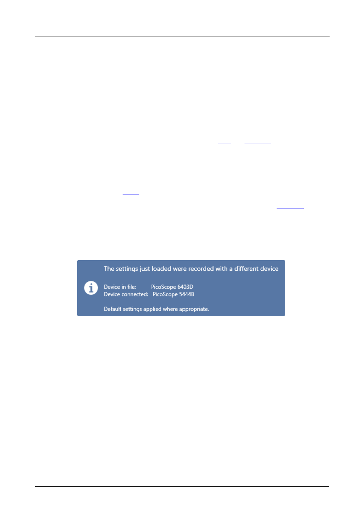
If you open a .psdata or .pssettings file that was saved using a different scope device from the one connected, PicoScope may need to modify the saved settings to suit the present device. A notification like the one below will appear in the bottom right corner of the PicoScope display:

Once you have opened a .psdata file, if you are using the default keyboard map, you can use the Page Up and Page Down keys to cycle through all the other data and settings files in the same directory.

Note: channel information for .psdata files is displayed in the Properties sheet. If a device is already connected when a .psdata file is loaded, the channel settings are changed to match the .psdata file where possible. The resulting settings are displayed on the Channels toolbar.

PicoScope 6 User's Guide 41

Location:

File > Save As...

Purpose:

allows you to save your waveforms and settings (including custom probes and active math channels) to a file in various formats

Data files (.psdata)

Stores waveforms and settings (including any custom probes, active math channels etc.) from the current scope device. Can be opened on any computer running PicoScope.

Settings files (.pssettings)

Stores all settings, including any custom probes, active math channels etc., from the current scope device. Does not save any waveform data. Can be opened on any computer running PicoScope.

CSV (Comma delimited) files (.csv)

Stores waveforms as a text file with comma-separated values. This format is suitable for importing into spreadsheets such as Microsoft Excel. The first value on each line is the time stamp, and it is followed by one value for each active channel, including currently displayed math channels. See Text

formats for more information.

5.1.3 Save As... dialog

PicoScope 6 Automotive only: the Options page of the Preferences dialog allows you to set the Details

dialog to appear before the Save As dialog, enabling you to record details about the vehicle and the

customer.

Type your chosen file name in the File name box, and then select a file format in the Save as type box. You can save data in the following formats:

Menus42

Text (Tab delimited) files (.txt)

Stores waveforms as a text file with tab-separated values. The columns are the same as those in the CSV format. See Text formats for more information.

Bitmap images (.bmp)

Stores pictures of the waveforms, graticule and rulers in Windows BMP format. The image is displayed in 16million colors and is uncompressed.

GIF images (.gif)

Stores pictures of the waveforms, graticule and rulers in CompuServe GIF format. The image is displayed in 256colors and is compressed.

Animated GIF image (.gif)

Creates an animated GIF that displays all of the waveforms in the buffer in sequence. Each waveform is formatted as in the single GIF format described above.

PNG images (.png)

Stores pictures of the waveforms, graticule and rulers in PNG format. The image is displayed in 16million colors, with lossless compression.

MATLAB 4 files (.mat)

Stores the waveform data in MATLAB 4 format.

JPEG (.jpg)

Stores pictures of the waveforms, graticule and rulers in JPG format. The image is displayed in 16million colors, with lossy compression.

PDF (.pdf)

Creates a PDF document with a images of each of the waveforms in the buffer, along with their graticules and rulers. There is one image on each page, displayed in 16million colors.

All waveforms

Saves all of the waveforms in the selected file format. If the file format is

.psdata, all of the waveforms are collected in a single file. You can then

load this into PicoScope and step through the waveforms using the buffer

navigation controls. If the selected file format does not support multiple

waveforms, PicoScope creates a new directory containing multiple files.

Current waveform only

Saves the single waveform that is currently on view.

Waveform numbers

Saves the specified list or range of waveforms. Each waveform is identified by its index number. For example:

1,2,9,10

2, 5-10

Options

The first three options control what happens when the waveform buffer contains more than one waveform:

5.1.3.1 File formats for exported data

PicoScope 6 can export raw data in either text or binary format:

Text-based file formats

Easy to read without special tools

Can be imported into standard spreadsheet applications

Files are very large if there are many samples in the data

PicoScope 6 User's Guide 43

There is no maximum file size when you export a text-based file, but not all editing applications can open large files. When you save a text-based file with more than 1million values per channel, PicoScope 6 will display the following warning:

Text file format details

Binary file format

Files remain relatively small and can even be compressed in some situations

Either a special application is required to read the files or the user must write a program to read the data from the file

Recommended for large data sets

Binary file format details

Data types for storing PicoScope 6 data

Regardless of whether the data types were loaded from a binary file or from a text-based file, we recommend the following data formats for storing the values loaded from a PicoScope 6 data file:

Sampled data (such as voltages) should use 32-bit single-precision floating-point data types

Times should use 64-bit double-precision floating-point data types

5.1.3.1.1 Text formats

Text-format files exported by PicoScope 6 are encoded in UTF-8 format by default. This is a popular format which is capable of representing a huge range of characters, whilst still retaining some compatibility with the ASCII character set if only standard Western European characters and numbers are used in the file.

CSV (comma-separated values)

CSV files store data in the following format:

Time, Channel A, Channel B (µs), (V), (V)

-500.004, 5.511, 1.215

-500.002, 4.724, 2.130

-500, 5.552, 2.212 …

There is a comma after each value on a line to represent a column of data and a carriage return at the end of the line to represent a new row of data.

Menus44

Time (µs)

Channel A (V)

Channel B (V)

500.004

5.511

1.215

-500.002

4.724

2.130

-500

5.552

2.212

…

ExtraSamples

the number of samples added, for example when filtering or resolution enhancement is enabled

RequestedLength

the number of samples. This will be the same as No. samples in the PicoScope 6

Properties sheet. Note that if the signal is not acquired in its entirety, this will be

different from Length.

Version

the exact version of PicoScope 6 used to export the file

Tab-delimited

Tab-delimited files store data in the following format:

The files have a tab character after each value on a line to represent a column of data and a carriage return at the end of the line to represent a new row of data.

5.1.3.1.2 Binary formats

PicoScope 6 can export data in version 4 of the .mat binary file format. This is an open format and the full specification is available as PDF documentation from the www.mathworks.com website. PicoScope 6 saves data into the MAT-file in a specific way, which is detailed below.

Note: data arrays saved in version 4 of the .mat file format must not exceed the maximum size of 100 million elements. MATLAB cannot read arrays with more elements than this in this format.

Importing into MATLAB

Load the file into your workspace using this syntax:

load myfile

Each channel’s data is stored in an array variable named by the channel. So, the sampled data for channels A to D would be in four arrays named A, B, C and D.

There is only one set of time data for all channels and this is loaded in one of two possible formats:

A start time, an interval and a length. The variables are named Tstart, Tinterval and Length.

An array of times (sometimes used for ETS data). The time array is named T.

If the times are loaded in as Tstart, Tinterval and Length then you can use the following command to create the equivalent array of times:

T = [Tstart : Tinterval : Tstart + (Length – 1) * Tinterval];

Note: the size of the largest file that MATLAB can open depends on the resources of the computer. It is therefore possible for PicoScope to create a MATLAB file that some installations of MATLAB would be unable to open. Please be aware of this risk when saving critical data.

The other three variables used in the file are:

PicoScope 6 User's Guide 45

Bytes

Value

0 to 3

Data format (0, 10 or 20)

4 to 7

Number of values

8 to 11

12 to 15

16 to 19

Name length

Value

Description

Double (64-bit floating point)

Single (32-bit floating point)

Integer (32-bit)

Exploring the file format

The full file specification, available from www.mathworks.com, is comprehensive so this guide does not describe the entire format. Instead, this guide describes enough of the format to allow you to get data from the file and use it in your own program.

The variables described above (under Importing into MATLAB) are stored in a series of data blocks, each preceded by a header. Each variable has its own header and data block and the corresponding variable names are stored with them (such as A, B, Tstart). The following sections describe how to read each variable from the file.

The order of the data blocks is not specified, so programs should look at the variable names to decide which variable is currently being loaded.

The header

The file consists of a number of data blocks preceded by 20-byte headers. Each header contains five 32-bit integers (as described in the table below).

Data format The Data format in bytes 0 to 3 describes the type of numerical data in the array.

Number of values

The Number of values is a 32-bit integer describing the number of numerical values in the array. This value may be 1 for variables that only describe one value; but for arrays of samples or times, expect this to be a large number.

Name length

The Name length is the length of the name of the variable as a null-terminated 1-byte per character ASCII string. The last null terminating character (\0) is included in the Name length so if the variable name is

Tstart (same as Tstart\0) then the name length will be 7.

The data block

The data block begins with the name of the variable (such as A, Tinterval) and you should read in the number of bytes described by the Name length part of the header (not forgetting that the last byte in the string is \0 if your programming language needs to take account of this).

The remaining part of the data block is the actual data itself, so read in the number of values described in the Number of values part of the header. Remember to take account of the size of each value as described in the ‘Data format’ part of the header.

Channel data such as voltages, in variables such as A and B, are stored as 32-bit single-precision floating- point data types. Times such as Tstart, Tinterval and T are stored as 64-bit double-precision floating-point data types. Length is stored as a 32-bit integer.

5.1.4 Start-up Settings menu

Location:

File > Start-up Settings

Purpose:

allows you to load, save and restore the PicoScope 6 startup settings

Save Settings As...

Stores all the current settings (for example collection time, input range, trigger), which can then be opened on any computer running PicoScope 6. This allows you to create a library of different setups.

Save User Default Settings

Saves the current settings as the default. This means you only have to configure the oscilloscope once in order to use these settings every time you open PicoScope 6.

Reset User Default Settings

This replaces your saved default settings with the original factory settings.

Load User Default Settings

Resets all settings to the saved default. You can also use the home button on the toolbar to achieve this.

Restore Last Session

This option returns the settings to those from your last session.

Load Factory Settings

Returns the settings to the factory original.

Load User Default Settings on Start-up

Selecting this option makes sure that the next time you start up PicoScope 6, the saved user default settings will be applied.

Restore Last Session on Start-up

You should check this box if you want PicoScope6 to open with the settings you used for your last session.

Menus46

PicoScope 6 User's Guide 47

Location:

File > Waveform Library Browser

Purpose:

allows you to search hundreds of user-uploaded waveforms by entering various fields of required data

Applicability:

PicoScope 6 Automotive only

Oscilloscope must be connected

5.1.5 Waveform Library Browser

Users of PicoScope Automotive oscilloscopes have access to the online Waveform Library. This is a collection of user-generated waveforms, with information about the vehicle under test. You can search the Waveform Library for waveforms from the vehicle and component you want to test, and also share your own examples. You can also treat the Waveform Library as an online backup for your own waveform files.

Once you have found a waveform, you can preview or open it. You can also use the waveform's individual channels as reference waveforms for your own signal, in PicoScope 6.

Menus48

Location:

Menu bar > Edit

Purpose:

gives access to the clipboard-related and note-editing functions

Copy as Image

Copies the active view to the clipboard as a bitmap. You can then paste the image into any application that accepts bitmap images.

Copy as Text

Copies the data in the active view to the clipboard as text. You can paste the data into a spreadsheet or other application. The text format is the same as that used by the Save As dialog when you select the .txt file type.

Copy Entire Window as Image

This copies a picture of the PicoScope window to the clipboard. It is provided as an alternative equivalent to pressing Alt + Print Screen for users of laptops without a Print Screen key. You can paste the picture into any application that can display pictures, such as a word processor or desktop publishing program.

Notes

Opens a Notes area at the bottom of the PicoScope window. You can type or paste your own notes in this area.

Details...

PicoScope 6 Automotive only. Opens the Details dialog, which allows you to enter or view vehicle details, customer details, notes and channel labels.

When you open the Waveform Library, a login page appears. Enter your username and password, and the software will take you to the page shown below.

The Waveform Library uses the same account information as the Pico automotive forum: if you are not already a member, you can register for free by following the link on the Waveform Library Login page.

5.2 Edit menu

PicoScope 6 User's Guide 49

Location:

Edit > Notes

Trigger toolbar > Other buttons > Notes button

Purpose:

provides a text box for typing your own notes

5.2.1 Notes

You can place a Notes area at the bottom of the PicoScope window, and you can enter any text you wish in it or paste text into it from other programs. This text is included when you save the waveform as a file.

5.2.2 Details dialog

Location:

File > Save As

Edit > Details

Purpose:

allows you to record channel labels and vehicle and customer details, before saving a file

Applicability:

PicoScope 6 Automotive only

Menus50

PicoScope 6 User's Guide 51

Location:

Edit > Details

Trigger toolbar > Other buttons > Channel Labels button

Purpose:

allows you to supply and view information on the waveforms

Applicability:

PicoScope 6 Automotive only

Label

Select a standard label from the drop-down list or type any text in the box.

Description

Type any text in the box to describe the waveform.

Status

Select Good, Bad or Unknown. This helps other engineers to identify whether the waveform is from a working engine or a faulty one.

You can enter information about the vehicle under test in the form shown above. You can also view and edit your notes and channel labels at the bottom of the PicoScope window by clicking the Notes and Channel Labels buttons in the Trigger toolbar.

Click the Customer tab to note down the customer's details. All of this information will be saved in the

.psdata file. You can then view it in PicoScope using the Edit > Details menu command.

5.2.2.1 Channel Labels

Channel labels can be displayed at the bottom of the PicoScope window.

5.3 Views menu

Location:

Menu bar > Views, or right-click on a view

Purpose:

controls the layout of the current view, which is a rectangular area of the PicoScope window that display scope, spectrum or other kinds of data

The contents of the Views menu may vary depending on where you click and how many views are open. If the current view contains a

Measurements table, a combined Measurements menu and Views

menu will appear.

Add View

Add a view of the selected type (scope, XY or spectrum). In automatic grid layout mode (the default), PicoScope rearranges the grid to make room for the new view, up to a limit of nine views. Any further views will be added as tabs in existing viewports. If you have selected a fixed grid layout, PicoScope will not change it.

Sub View

Mixed signal oscilloscopes only: switch the analog view and digital view on and

off independently

Rename View

Change the standard Scope or Spectrum label to a title of your choice

Close View

Remove a view from the PicoScope window. In automatic grid layout mode (the default), PicoScope rearranges the grid to make the best use of the remaining space. In fixed grid layout mode (if you have selected a fixed grid layout), PicoScope will not change the grid.

Channels

Select which channels are visible in the current view. Each view, when created, shows all the input channels, but you can switch them on and off using this command. Only the input channels that are enabled (not set to Off in the

Channel Setup Toolbar) are available for viewing. The Channels menu also list math channels and reference waveforms. You can select up to 8 channels in any

view.

Menus52

PicoScope 6 User's Guide 53

X-Axis

Select any suitable channel to drive the X axis. By default, the X axis represents time. If you select an input channel instead, the scope view will become an XY

view that plots one input against another. A quicker way to create an XY view is

to use the Add View command (see above).

Grid Layout

The grid layout defaults to Automatic mode, in which PicoScope automatically arranges viewports in a grid. You can also select one of the standard grid layouts or create a custom layout, which PicoScope will preserve as you add or remove views.

Arrange Grid Layout

Adjust the grid layout to fit the number of views. Moves any tabbed views to empty viewports. Overrides any previous choice of grid layout.

Reset View Sizes

If you have resized any of the views by dragging the vertical or horizontal separator bars between viewports, this option resets all the viewports to their original sizes.

Move View To

Move a view to a specified viewport. You can achieve the same effect by dragging the view by its name tab and dropping it in a new viewport: see How to

move a view.

Arrange Views

If multiple views are stacked in the same viewport, move them into their own viewports

Auto-arrange axes

Scale and offsets all traces to fill the view and avoid overlaps

Reset View Layout

Reset the scale factor and offset of the selected view to their default values

View Properties

Show the Properties sheet, which lists scope settings that are normally hidden

Location:

Views menu > Grid Layout > Custom layout...

Purpose:

if the Grid Layout section of the Views menu does not contain the layout you want, this dialog gives further options

5.3.1 Custom grid layout dialog

You can lay out the view grid with any number of rows and columns up to 4 by 4. You can then drag the views to different locations in the grid.

5.4 Measurements menu

Location:

Menu bar > Measurements

Purpose:

controls the Measurements table

Add Measurement. Adds a row to the measurements table, and opens the Add Measurement

dialog.

Edit Measurement. This takes you to the Edit Measurement dialog. You can also edit a measurement by double-clicking on a row of the measurements table.

Delete Measurement. Removes the selected row from the measurements table.

Grid Font Size. Sets the font size for the entries in the measurements table.

Column Auto-width. If this box is checked, the columns of the measurements table will

continually adjust to fit the contents whenever the table changes. Click again to release the button.

DeepMeasure™. Allows you to make and analyze a number of automatic measurements over up to 1 million individual cycles.

Menus54

You can also access the Add Measurement, Edit Measurement and Delete Measurement commands from the Measurements buttons, on the Trigger toolbar, or by right-clicking on a view.

PicoScope 6 User's Guide 55

Location:

Trigger toolbar > Measurements buttons > Add Measurement or Edit

Measurement button

Measurements menu > Add Measurement or Edit Measurement button

Double-click a measurement in the measurements table

Purpose:

allows you to add a measurement of a waveform to the selected view, or edit an existing

measurement

5.4.1 Add/Edit Measurement dialog

If this is the first measurement for the active view, PicoScope will create a new measurements table; otherwise, it will add the new measurement to the bottom of the existing table. PicoScope automatically refreshes the measurement every time it updates the waveform.

Select the channel to measure

Choose which of the scope device's channels to measure.

Select the type of measurement

PicoScope can calculate a wide range of measurements for waveforms. See scope measurements (for use with scope views) or spectrum measurements (for use with spectrum views) for a list.

Choose which section of the graph will be measured

Measure the whole trace, the section between two time or frequency rulers or a single cycle marked by one ruler.

Measurement Options

Some measurements have additional settings to choose from: see Scope measurement options and

Spectrum measurement options for more information.

5.4.1.1 Scope measurement options

Threshold and hysteresis (Edge Count, Falling Edge Count and Rising Edge Count only)

Menus56

Use these options to control the threshold method and the degree of hysteresis for Edge Count, Falling Edge Count and Rising Edge Count measurements.

Threshold (Falling Rate, Fall Time, Rise Time and Rising Rate only)

Falling Rate, Fall Time, Rise Time and Rising Rate measurements can be made with different thresholds. Use this control to select one.

When comparing rise and fall times with manufacturers' specifications, it is important to use the same thresholds for all measurements.

PicoScope 6 User's Guide 57

5.4.1.2 Spectrum measurement options

Spectrum Span (all Spectrum measurements)

When measuring peak-related parameters in a spectrum view, PicoScope can search for a peak near the specified frequency ruler location. This option tells PicoScope how many frequency bins to search.

Harmonic control options (Total Harmonic Distortion [all variants], SINAD and Signal to Noise Ratio [SNR] only)

The following options apply to distortion measurements. You can specify which harmonics PicoScope uses for these measurements.

Highest Harmonic

The highest harmonic to include when calculating distortion power.

Search Range

The number of frequency bins to search, centered on the expected frequency, when looking for a harmonic peak.

Harmonic Noise Floor

The level in dB above which signal peaks will be counted as harmonics.

5.4.2 DeepMeasure™ dialog

Location:

Measurements > DeepMeasure

Purpose:

lets you set up which channel to use for DeepMeasure

Menus58

Adding a new instance of DeepMeasure

1. Make sure the channel you want to measure is enabled, using the Channels toolbar.

2. Click the Create button.

3. This opens the DeepMeasure Settings dialog: use this to select which channel to measure and define the

waveform cycles and how you would like to view the data.

4. Click OK. The new instance of DeepMeasure will appear in the list, as shown above, where you can edit or

delete it, or add more.

PicoScope 6 User's Guide 59

Data

The input channel to measure

Cycle Threshold

The signal level that defines the beginning and end of the cycle. The signal will cross this threshold three times in every cycle.

Cycle Hysteresis

Eliminates the effect of noise on the Cycle Threshold, in a similar way to trigger

hysteresis. The value you enter here is a range, to be divided equally either side of

the threshold.

Rise/Fall Time Threshold

High and low measurement thresholds as a percentage of waveform height, excluding ringing. Choose lower and upper step values of 10/90 or 20/80.

Name

Enter a name for this instance of DeepMeasure. This is optional, but can be useful if you set up more than one instance for the same channel.

If you do not enter a name, PicoScope will generate one automatically.

Display cycles in

Graph: Enables the DeepMeasure overlay.

Between time rulers: Only measures the section of waveform shown between the

time rulers.

5.4.2.1 DeepMeasure™ Settings

Use this dialog to set up the channel and waveform characteristics to measure, and set up the display options.

Channels

Display

Menus60

5.4.2.2 DeepMeasure™ data window

When you use DeepMeasure, PicoScope automatically displays the measurement data in a table below your waveform, as shown below. You can sort this data by any of the fields.

Double-click one of the waveform cycles in the scope view to zoom in on it and go to the corresponding row in the table, or double-click a row in the table to zoom in on the selected cycle in the scope view.

DeepMeasure overlay

This feature highlights individual waveform cycles in the graph.

Boundaries between cycles are marked with thick black lines.

Each cycle is numbered so you can easily match the waveforms in the graph to the entries in the data table.

Hover the mouse pointer over any cycle to display a summary of its measurements.

Double-click any cycle in the graph or the data table to highlight it in the graph and zoom on it, and to highlight it in the data table.

DeepMeasure tabs

Each instance of DeepMeasure is displayed in a separate table. Use these tabs to switch between them.

PicoScope 6 User's Guide 61

Open the DeepMeasure Settings dialog

Export

Save the decoded data in a link file, as an OpenDocument Spreadsheet (ODS) or Comma-Separated Values (CSV) text file

View

Fields: Choose which data fields are displayed

Grid Font Size: Change the size of the characters in the table

Buffer

Choose whether to display packets from the Current Buffer or All Buffers

Location:

Menu bar > Tools

Purpose:

gives access to assorted tools for signal analysis

Custom Probes. Define new probes and copy, delete, move and edit existing ones.

Math Channels. Add or edit a channel that is a mathematical function of one or more other

channels.

Reference Waveforms. Create, load or save a channel as a copy of an existing channel.

Serial Decoding. Decode and display the contents of serial data streams such as CAN bus.

Alarms. Specify actions to be taken on certain events.

Masks. Perform mask limit testing on a waveform. This detects when the waveform departs from

a specified shape.

Control bar

Fields

Each field in the data table represents one type of measurement.

Click and drag the edges of each column to change the width, and make viewing the field data clearer.

Click the field header to sort the table by that field, in ascending order. Click again to sort in descending order.

5.5 Tools menu

Menus62

Macro Recorder. Save a frequently-used sequence of operations.

Preferences. Set various options that control PicoScope's behavior.

PicoScope 6 User's Guide 63

Location:

Tools > Custom Probes

or open it from the Channel Options menu:

Purpose:

allows you to set up and edit custom probes

5.5.1 Custom Probes dialog

The selection of built-in probes shown may vary depending on the version of the PicoScope software that you are using.

Understanding the probe list All the probes that PicoScope knows about are listed under three main headings: Built-in, Library and

Loaded. The probe list is preserved between sessions, so that PicoScope will never forget your custom

probes unless you delete them.

Built-in probes. The built-in probes are supplied by Pico Technology and do not change unless you download an authorized update from us. As a safeguard, PicoScope does not allow you to edit or delete these probes. If you want to modify one of them, you can copy it to your library by clicking Duplicate, and then edit the copy in your library.

Library probes. These are the probes that you have created using any of the methods described in this topic. You can edit, delete or duplicate any of these probes by clicking the appropriate button in this dialog.

Loaded probes. Probes in PicoScope data files (.psdata) or settings files (.pssettings) that you have opened appear here until you copy them to your library. You cannot edit or delete these probes directly, but you can click Save to Library to copy them to your library where you can edit them.

Adding a new probe to your library

There are three ways to create a new probe:

Use the Duplicate button as described above.

Click New Probe... to define a new probe.

Click Import to load a probe definition from a *.psprobe file and add it to your library. These files are normally supplied by Pico, but you can also create your own by defining a new probe and then clicking Export.

The last two methods open the Custom Probe wizard to guide you through the probe definition process.

5.5.1.1 Custom Probe wizard

Location:

Custom Probes dialog > New Probe

Purpose:

allows you to define custom probes and set up custom ranges

1. Introduction or Edit

2. Probe output units

3. Scaling method

The first dialog in the series is either the Custom Probe wizard introduction dialog or the Edit an existing

Custom Probe dialog.

Menus64

PicoScope 6 User's Guide 65

4. Range management

5. Manual ranges setup

6. Filter method

7. Custom probe identification

5.5.1.1.1 Custom Probe wizard introduction dialog

Location:

Custom Probes dialog > New Probe...

Purpose:

introduces you to the process for creating a new custom probe

Menus66

Click Next to continue to the Probe Output Units dialog.

PicoScope 6 User's Guide 67

Location:

Custom Probes dialog > Edit...

Purpose:

introduces you to the process for editing an existing custom probe

5.5.1.1.2 Edit Existing Custom Probe dialog

Click Next to continue to the Probe Output Units dialog.

5.5.1.1.3 Probe Output Units dialog

Location:

Custom Probe wizard

Purpose:

allows you to choose the units that PicoScope will use to display the output of your custom

probe

Menus68

To choose a standard SI unit, click Use a standard unit from the list and select one from the list.

To enter a custom unit, click Use the custom unit defined below and type the unit name and symbol.

Click Next to continue to the Scaling Method dialog.

Click Back to return to the Custom Probe wizard introduction dialog if this is a new probe, or the Edit Existing

Custom Probe dialog if this is an existing probe.

PicoScope 6 User's Guide 69

Location:

Custom Probe wizard

Purpose:

allows you to define the characteristic that PicoScope will use to convert the custom probe's voltage output to a measurement on the display

5.5.1.1.4 Scaling Method dialog

If you do not require any scaling or offset, select Don't apply any scaling to the data.

If the probe requires linear scaling, select Use a linear equation to scale the data and enter the gradient (or scale factor) m and the offset c in the equation y = mx + c, where y is the displayed value and x is the probe's voltage output.

If you wish to apply a nonlinear function to the probe's output, choose Use a look-up table, then click the Create a Lookup Table... button to create a new lookup table. This will take you to the Lookup-table Scaling

dialog.

Click Next to continue to the Range Management dialog.

Click Back to return to the Probe Output Units dialog.

5.5.1.1.4.1 Lookup-table Scaling dialog

Location:

Custom Probe wizard > Scaling Method dialog > Create a Lookup Table... or Edit the

Lookup Table...

Purpose:

creates a lookup table to calibrate a custom probe

Menus70

Editing the Lookup Table

First, select suitable values in the Input units and Scaled units drop-down boxes. For example, if your probe is a current clamp that outputs one millivolt per ampere over the range –600 to +600 amperes, select Input units of millivolts and Scaled units of amperes.

Next, enter some data in the scaling table. Click the first empty cell at the top of the table and type –600, then hit the Tab key and type –600. When you are ready to enter the next pair of values, press the Tab key again to start a new row. You can also right-click on the table to obtain a more detailed menu of options, as

shown in the picture. In the example above, we have entered a slightly nonlinear response; if the response had been linear then it would have been easier to use the linear option in the Scaling Method dialog.

Import.../Export...

Using the Import... button, you can fill the lookup table from data in a comma-separated or tab-delimited text file. The Export... button allows you to save the lookup table to a new file.

Finishing Clicking OK or Cancel will return you to the Scaling Method dialog.

PicoScope 6 User's Guide 71

Location:

Custom Probe wizard

Purpose:

allows you to override PicoScope's automatic range-creation feature for custom probes. In most cases, the automatic procedure will be sufficient.

What is Auto-ranging?

When the Auto-ranging function is selected, PicoScope continually monitors the input signal and adjusts the range when necessary to allow it to display the signal with maximum resolution. This function is available on all standard ranges, and can be used with custom ranges if you select Let the software manage my ranges for me automatically in this dialog.

5.5.1.1.5 Range Management dialog

If you select Let the software manage my ranges for me automatically, clicking Next will take you to the

Custom Probe Identification dialog. PicoScope's automatic ranges should be ideal for most applications.

If you select I will manage the Custom Probe Ranges manually, clicking Next will take you to the Manual

Ranges Setup dialog.

Click Back to return to the Scaling Method dialog.

5.5.1.1.6 Manual Ranges Setup dialog

Location:

Custom Probe wizard > Range Management dialog > Advanced > Next

Purpose:

creates ranges manually for your custom probe

Menus72

If you wish, you can click Auto Generate Ranges and the software will create a number of ranges for the selected device. This will create the same list of ranges that you would have obtained by selecting Let the software manage my ranges for me automatically in the previous dialog. When you select a range, a diagram below the list will show its relationship to the scope device's input range – this is explained further under Edit range dialog. You can then edit the ranges by clicking Edit, or you can also add a new range by clicking New Range. Both of these buttons take you to the Edit Range dialog.

Click Next to continue to the Filter Method dialog.

Click Back to return to the Range Management dialog.

PicoScope 6 User's Guide 73

Here is the standard input range menu for the built-in x1 probe:

When you create a custom input range, it appears in the drop-down list of ranges in the channels toolbar, like this:

How to use a new custom range

Menus74

Location:

Custom Probe wizard > Range Management dialog > Manual Ranges Setup dialog > Edit

Range or New Range

Purpose:

editing a manual range for a custom probe

5.5.1.1.6.1 Edit Range dialog

An input range is the signal range, usually in volts, on the input channel of the scope device. The scaled range is the range that will appear on the vertical axis of the scope display when the probe is selected. Your scaled range should match the input range as closely as possible, to make the most of the scope's resolution.

The scaling that you chose on the Scaling Method page defines the relationship between the input range and the scaled range. This dialog enables you to set up ranges to display the scaled data on the scope view.

Standard Options tab

Automatically select the hardware input range for the range limits I specify below

If you leave this radio button pressed, PicoScope will automatically determine the best hardware input range for the device as you change the Scaled range limits. This is the best mode to use for almost all ranges. You should set the Scaled range limits to the maximum and minimum values you wish to see on the vertical axis of the scope display.

Use this hardware input range

If you press this radio button and select a hardware input range from the drop-down box, PicoScope will then use that hardware input range whatever scaled range limits you choose. Set the upper and lower scaled range limits to the limits you wish to appear at the top and bottom of the vertical axis in PicoScope's scope

view.

The range utilization bar

This diagram at the bottom of the dialog shows how well the input range of the device is matched to the scaled range.

PicoScope 6 User's Guide 75

Green - The section of the input range that is used by the scaled range. This should be as large as

possible, to maximize the use of the scope device's resolution.

Blue - Areas of the input range that are not being used. These indicate wasted resolution.

Grey - Parts of the scaled range that are not covered by the input range. These will result in wasted space

on the graph. The range utilization bar may not represent these areas accurately when non-linear scaling is being used, so you should always test the scaled range limits on the scope view.

Advanced tab

The Advanced tab allows you to configure advanced options for custom probes. However, these options are for factory use and we recommend that you do not change them.

Finishing Clicking OK or Cancel will return you to the Manual Ranges Setup dialog.

5.5.1.1.7 Filter Method dialog

Location:

Custom Probe wizard

Purpose:

sets up lowpass filtering for this custom probe

Menus76

This dialog has the same effect as manually enabling the Lowpass Filtering option in the Channel Options

dialog. Filtering will only occur if the attached scope device supports filtering.

Click Back to go to the Manual Range Setup dialog.

Click Next to go to the Custom Probe Identification dialog.

PicoScope 6 User's Guide 77

Location:

Custom Probe wizard

Purpose:

entering text to identify the custom probe

5.5.1.1.8 Custom Probe Identification dialog

Click Back to return to the Filter Method dialog.

The probe name will appear in the probe list.

The optional description is not used in the current version of the software.

Click Finish to accept your custom probe settings and return to the Custom Probes dialog.

5.5.2 Math Channels dialog

Location:

Tools > Math Channels

Purpose:

creating, editing and controlling math channels, which are virtual channels generated by

mathematical functions of input channels

Math Channel list

The main area of the Math Channels dialog is the Math Channel list, which shows all the built-in, library and loaded math channels. To choose whether or not a channel appears in the main PicoScope window, click the appropriate check box and then OK. You can have up to eight channels in any view, including input channels and math channels. If you enable a ninth channel, PicoScope opens a new view.

Built-in: these math channels are defined by PicoScope and cannot be changed.

Library: these are the math channels that you define using the Create, Duplicate or Edit buttons, or load with the Import button.

Loaded: these are the math channels present in any PicoScope settings or data files

that you have loaded.

Create

Opens the Math Channel wizard, which guides you through the process of creating or editing a math channel. The new channel will appear under Library in the Math

Channel list.

Edit

Opens the Math Channel wizard to allow you to edit the selected math channel. You must first select a channel in the Library section of the Math Channel list. If the channel you want to edit is in the Built-in or Loaded section, first copy it to the

Library section by clicking Duplicate, then select it and click Edit.

Menus78

PicoScope 6 User's Guide 79

Delete

Permanently deletes the selected math channel. Only math channels in the Library section can be deleted.

Duplicate

Creates a copy of the selected math channel. The copy is placed in the Library section, where you can edit it by clicking Edit.

Import

Opens a .psmaths math channel file and places the math channels it contains in the Library section.

Export

Saves the highlighted math channel from the Library section to a new .psmaths file.

Location:

Channel Setup toolbar > Math Channels button

Purpose:

creating, editing and controlling math channels, which are virtual channels generated by mathematical functions of input channels

1. Introduction

2. Equation

5.5.2.1 Math Channel wizard

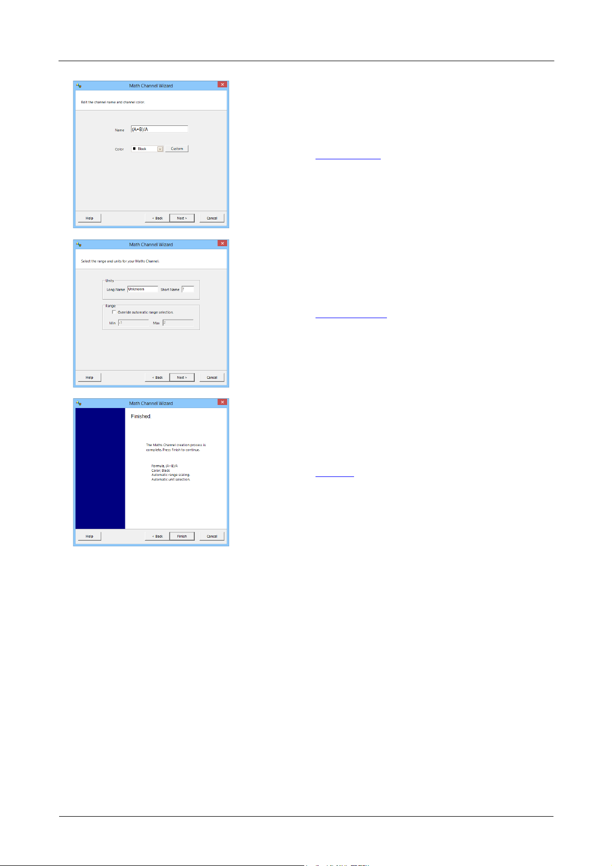
Menus80

3. Channel name

4. Units and range

5. Finished

PicoScope 6 User's Guide 81

Location:

Math Channels dialog > Create

Purpose:

introduces you to the process for creating a new math channel

5.5.2.1.1 Math Channel wizard introduction dialog

Click Next to continue to the Math Channel wizard Equation dialog.

Menus82

Location:

Math Channel wizard

Purpose:

allows you to enter or edit the equation for a math channel

Math Channel wizard Equation dialog, basic view

Button

Equation

Description

Clear Equation. Clears the entire contents of the equation box.

Clear. Clears the single character to the left of the cursor.

Add

5.5.2.1.2 Math Channel wizard Equation dialog

You can type directly into the equation box, or click the calculator buttons and let the program insert the symbols for you. A red error indicator will appear to the right of the equation box if the equation contains

a syntax error.

When you are happy with your equation, click Next to continue to the Math Channel wizard Name dialog.

Basic view

Basic buttons

PicoScope 6 User's Guide 83

–

Subtract (or negate)

Multiply

Divide

...

A...D

Input Channels. The selection available depends on the number of enabled channels on the scope device.

{...}, T

Other Operands. Shows a drop-down list of available inputs to equations, including reference waveforms and Time.

(...)

Brackets. Expressions within brackets will be evaluated before the expressions to either side.

Math Channel wizard Equation dialog, advanced view, showing Main group of buttons

Advanced view

Clicking the Advanced button reveals more function buttons. Initially these are the Main group of buttons, as shown below.

Advanced buttons (numeric keypad)

Button

Equation

Description

...

0..9

0 to 9. The decimal digits.

Decimal point

Exponent. aEb means a × 10b.

Button

Equation

Description

Power. Raise x to the power of y.

ln()

Natural logarithm

exp()

Natural exponent. Raise e, the base of the natural logarithm, to the power ofx.

freq()

Frequency. Calculated in hertz.

duty()

Duty. Calculate the duty cycle as a percentage.

log()

Logarithm. Base-10 logarithm.

derivative()

Derivative. Calculated with respect to the x-axis.

Note: the derivative of a sampled signal contains a large amount of noise, so it is advisable to apply digital lowpass filtering to all channels used as inputs to this function.

integral()

Integral. Along the x-axis.

sqrt()

Square root

norm()

Normalize. PicoScope calculates the maximum and minimum values of the argument over the capture period, and then scales and offsets the argument so that it exactly fits the range [0, +1] units.

abs()

Absolute value

crank()

Crank speed (PicoScope Automotive only). This function requires two arguments: the channel, and the number of teeth on the crank sensor (including the spaces for missing teeth). PicoScope then calculates and plots the crank speed in RPM.

Advanced buttons (Main group)

Menus84

PicoScope 6 User's Guide 85

Button

Equation

Description

Pi. The ratio of a circle's circumference to its diameter.

Inverse. Modifies the sin, cos and tan buttons to the inverse trigonometric

functions asin, acos and atan.

sin()

Sine. The operand is in radians.

cos()

Cosine. The operand is in radians.

tan()

Tangent. The operand is in radians.

sinh()

Hyperbolic sine.

cosh()

Hyperbolic cosine.

tanh()

Hyperbolic tangent.

Button

Equation

Description

min()

Minimum. Negative peak detect of all previous waveforms.

max()

Maximum. Positive peak detect of all previous waveforms.

average()

Average. Arithmetic mean of all previous waveforms.

peak()

Peak detect. Display maximum-to-minimum range of all previous waveforms.

Button

Equation

Description

HighPass(i,f)

Highpass filter. Attenuates low frequencies.

Click Trigonometric, Buffered, Filters or Coupler to reveal alternative groups of buttons:

Advanced buttons (Trigonometric group)

Advanced buttons (Buffered group)

When the scope is running, these functions operate continuously on all waveforms since the scope started capturing. If a math channel containing these functions is enabled when the scope is stopped, it operates on the contents of the waveform buffer instead.

Advanced buttons (Filters group)

Parameters:

i is the input channel or other operand (see under Basic buttons above) f (or f1 and f2) are the –3 dB cutoff frequencies of the filter, in hertz

Menus86

Button

Equation

Description

LowPass(i,f)

Lowpass filter. Attenuates high frequencies.

BandPass(i,f1,f2)

Bandpass filter. Attenuates high and low frequencies outside the specified range.

BandStop(i,f1,f2)

Bandstop filter. Attenuates mid-band frequencies inside the specified range.

Button

Equation

Description

Coupler(s1,s2,RG58,d)

RG58 coupler. For coaxial cables.

Coupler(s1,s2,Cat5,d)

Cat5 coupler. For twisted-pair cables.

These are digital filters with a finite number of taps and therefore cannot attenuate down to DC. They have a minimum cutoff frequency of 1/64 000 of the scope's sampling rate. You can find the current sampling rate displayed in the Properties sheet.

Advanced buttons (Coupler group)

Parameters:

s1 is the master channel s2 is the slave channel d is the distance between the master and slave probing points, in metres

These are directional coupler functions for extracting BroadR-Reach signals from a bidirectional bus. One differential probe (connected to channel s1) is placed on the cable near the master device, and another

(connected to channel s2) on the cable near the slave device. The output of the coupler is then used as the input to the BroadR-Reach protocol decoder (see Serial Decoding).

Additional functions

There are a few operators that can be entered only by using the equation box:

Signum function. The sign() operator returns the sign of its input. The result is +1 when the input is positive, –1 when the input is negative, and 0 when the input is 0.

Advance/Delay. To deskew a signal, select the channel and add the deskew time in seconds, in square brackets. For example, to advance Channel A by 1millisecond, enter A[0.001], and to delay Channel A by 1millisecond, enter A[–0.001]. Using time offsets to adjust one channel relative to another can compensate for differences in cable lengths or skew in trace lengths.

PicoScope 6 User's Guide 87

Location:

Math Channel wizard

Purpose:

allows you to enter or edit the name and color of a math channel

5.5.2.1.3 Math Channel wizard Name dialog

PicoScope initially sets the name to the text of the equation, but you can edit it to anything you like. The name will appear in the channel list in the Math Channels dialog. You can set the color of the trace to one of the standard colors in the drop-down-list, or click Custom to choose any possible color allowed by Windows.

Click Next to continue to the Math Channel wizard Units and Range dialog.

5.5.2.1.4 Math Channel wizard Units and Range dialog

Location:

Math Channel wizard

Purpose:

allows you to specify the measurement units and the range of values to display for a math

channel

Menus88

Units Long Name: This is for your reference only.

Short Name: This will be displayed on the vertical axis in scope and spectrum views, in the ruler legend and

in the measurements table.

Range

If you leave the Override automatic range selection check box empty, PicoScope will choose the most appropriate range for the vertical axis. If you prefer to set your own minimum and maximum values for the axis, check the box and enter them in the Min and Max boxes.

Click Next to continue to the Math Channel wizard Finished dialog.

PicoScope 6 User's Guide 89

Location:

Math Channel wizard

Purpose:

shows you the settings for the math channel that you have just created or edited

5.5.2.1.5 Math Channel wizard Finished dialog

Click Back to return to previous dialogs in the Math Channel wizard if you wish to change any of the settings.

Click Finish to accept the settings shown and return to the Math Channels dialog. If you want the new or edited channel to appear on the scope or spectrum display, remember to check the appropriate box in the channel list. You can change them later by returning to the Math Channels dialog.

5.5.3 Reference Waveforms dialog

Location:

Tools > Reference Waveforms

Purpose:

enables you to create, edit and control reference waveforms, which are stored copies of input channels

Reference Waveforms list

The main area of the Reference Waveforms dialog is the Reference Waveforms list, which shows all the available input channels and the library and loaded reference

waveforms. To choose whether or not a waveform appears in the main PicoScope window, click the appropriate check box and then OK. You can have up to eight

channels in any view, including input channels, math channels and reference waveforms. If you try to enable a ninth channel, PicoScope will open another view.

Available: these input channels are suitable as sources for reference waveforms

Library: these are the reference waveforms that you have defined using the Duplicate button or loaded with the Import button

Loaded: these are the reference waveforms present in any PicoScope settings or

data files that you have loaded

Edit

Opens the Edit Reference Waveform dialog to allow you to edit the selected reference waveform. You must first select a waveform in the Library section of the Reference Waveforms list. If the waveform you want to edit is in the Loaded section, first copy it to the Library section by clicking Duplicate, then select it and click Edit.

Delete

Permanently deletes the selected reference waveform. Only reference waveforms in the Library section can be deleted.

Menus90

PicoScope 6 User's Guide 91

Duplicate

Creates a copy of the selected input channel or reference waveform. The copy is placed in the Library section, from where you can edit it by clicking Edit. A quicker way to do the same thing is to right-click on the view, select Reference Waveforms and then click the channel that you wish to copy.

Import

Opens a .psreference reference waveform file and places the waveforms it contains in the Library section.

Export

Saves the highlighted reference waveform from the Library or Loaded sections to a new .psreference or MATLAB 4 .mat file.

Location:

Reference Waveforms dialog > Edit

Purpose:

allows you to edit the name and color of a reference waveform

Name:

PicoScope initially names the waveform after the input channel used as its source, but you can edit it to anything you like. Here we have named it noise. The name will appear in the waveform list in the Reference Waveforms dialog.

Color:

You can set the color of the trace to one of the standard colors in the drop-down-list, or click Custom to choose any color allowed by Windows.

5.5.3.1 Edit Reference Waveform dialog

5.5.4 Serial Decoding dialog

Location:

Tools > Serial Decoding

Purpose:

lets you set up which channels and protocols to use for serial decoding

Menus92

Adding a new serial decoder

1. Make sure the channel you want to decode is enabled, using the Channels toolbar. For duplex protocols

such as UART, you must decode each direction (for example Tx and Rx) using a separate channel.

2. Click the Create button, as shown above, and select the serial decoding protocol you would like to use

from the list.

3. This opens the Decoder Settings dialog: use this to select which channel to decode and how you would

like to view the data, and to adjust other settings. Each protocol has different settings to adjust.

4. Click OK. Your selected protocols will appear in the Serial decoders list, as shown above, where you can

edit or delete them.

PicoScope 6 User's Guide 93

Data

Data channel for various protocols.

Note: Bidirectional SPI can be decoded as two separate buses, one with Data In (DI) as the I/O signal and the other with Data Out (DO) as the I/O signal. The Clock (and Chip Select if present) can be shared by both buses.

Differential signal

Coupler output for BroadR-Reach decoding. First create a Coupler math

channel, then select this channel as the input to the decoder.

Tx (Master)

Master signal for Modbus protocols

Rx (Slave)

Slave signal for Modbus protocols

Clock

Clock for various protocols

Word Select

For the I2S protocol. Indicates which stereo channel the data belongs to.

Chip Select

For the SPI protocol. If there is no Chip Select signal, clear the check box.

DataPlus and DataMinus

For the USB (1.0/1.1) protocol.

5.5.4.1 Decoder Settings

Different settings options are available for each protocol decoder.

If the serial decoding parameters entered are incorrect, PicoScope will display an error message.

Channels

Signals

Controls

Invert

Reverses the polarity of the signal

Threshold

The voltage that defines the transition in either direction between high and low logic states

Hysteresis

Eliminates the effect of noise on the threshold, in a similar way to trigger

hysteresis. The value you enter here is a range, to be divided equally either side

of the threshold.

Baud Rate

The symbol frequency in baud. PicoScope will automatically detect the baud rate and select a value for you. Alternatively, you can choose one of the standard values from the drop-down list or enter an arbitrary value.

Bit Order

Whether the most or least significant bit occurs first.

For protocols with application-specific bit order, such as UART, you must set this to match to the data format.

Bus Speed

The maximum data rate of the I2C serial bus

Checksum Length

The number of words following the data field to decode as the checksum.

Chip Select State

The polarity of the Chip Select (CS) signal

Clock Edge

Whether to sample the clock (SCK) on the falling or rising edge

Data Bits

The number of bits in the data payload of each packet

Data Bit Rate

The bit rate (in baud) of the data phase of the signal, independent of bit encoding and decoding

Data Encoding

Encoding of the ARINC 429 data field: binary coded decimal (BCD), binary number representation (BNR), or discrete data representation

Data Length

The number of words decoded as the data field following the header.

Data Length Type

Fixed: The data field is a fixed length as specified. Used in protocols such as

MIL-STD-1553. Remaining: The data field is a variable length, equal to the packet length minus the lengths of the other fields. Used in protocols such as Ethernet 10BaseT.

Display 4B/5B Code Groups

Show the 4B/5B block coding scheme output (rather than Ethernet packets) for the Fast Ethernet protocol

End Of Packet Byte

For the Modbus ASCII protocol. Byte value of the line feed (LF) byte.

First Slot

The first DMX channel to display

Full-speed (12 Mbit/s)

Full speed USB 1.0 or 1.1 protocol

Header Length

The number of words decoded as the packet header after the preamble.

High or Low

The signal polarity of the CAN or CAN FD protocol

Configuration

Menus94

PICO PS 4224A User guide

Specifications and Main Features

Frequently Asked Questions

User Manual

1 Welcome

Introduction4

2.1 Legal statement

2.2 Updates

2.3 Trademarks

2.4 System requirements

Using PicoScope for the first time6

4 PicoScope and oscilloscope primer

4.1 Oscilloscope basics

4.2 PC Oscilloscope basics

4.3 PicoScope basics

4.3.1 Capture modes

See also How do capture modes work with views?

4.4 PicoScope window

4.5 Scope view

4.6 Overrange indicator

4.7 MSO view

right-click on the digital view

Note 1: you can right-click on the digital view to obtain the Digital context menu.

4.8 XY view

4.9 Trigger marker

4.10 Time-delay arrow

4.11 Spectrum view

Persistence mode superimposes multiple waveforms on the same view, with more frequent data or newer waveforms drawn in brighter colors than older ones. This is useful for spotting glitches, when you need to see a rare fault event hidden in a series of repeated normal events.

4.13 Measurements table

4.14 DeepMeasure™

4.15 Pointer tool tip

4.16 Signal rulers

4.17 Time and frequency rulers

4.18 Phase (rotation) rulers

4.19 Ruler settings

4.20 Ruler legend

See also frequency legend.

4.22 Properties sheet

4.23 Custom probes

4.24 Math channels

4.25 Reference waveforms

4.26 Serial decoding

4.27 Mask limit testing

4.28 Alarms

4.29 Buffer Overview

Menus36

5.1 File menu

5.1.1 Connect Device dialog

5.1.1.1 Demo mode

5.1.2 Open dialog

5.1.3 Save As... dialog

5.1.3.1 File formats for exported data

5.1.3.1.1 Text formats

5.1.3.1.2 Binary formats

5.1.4 Start-up Settings menu

5.1.5 Waveform Library Browser

5.2 Edit menu

5.2.1 Notes

5.2.2 Details dialog

5.2.2.1 Channel Labels

5.3 Views menu

5.3.1 Custom grid layout dialog

5.4 Measurements menu

5.4.1 Add/Edit Measurement dialog

5.4.1.1 Scope measurement options

5.4.1.2 Spectrum measurement options

5.4.2 DeepMeasure™ dialog

5.4.2.1 DeepMeasure™ Settings

5.4.2.2 DeepMeasure™ data window

5.5 Tools menu

5.5.1 Custom Probes dialog

5.5.1.1 Custom Probe wizard

5.5.1.1.1 Custom Probe wizard introduction dialog

5.5.1.1.2 Edit Existing Custom Probe dialog

5.5.1.1.3 Probe Output Units dialog

5.5.1.1.4 Scaling Method dialog

5.5.1.1.5 Range Management dialog

5.5.1.1.6 Manual Ranges Setup dialog

5.5.1.1.7 Filter Method dialog

5.5.1.1.8 Custom Probe Identification dialog