PICO PicoVNA 106 User Manual

Download

PicoVNA™ 106

Vector Network Analyzer

User's Guide

pv106ug r1

Distribution in the UK & Ireland

Lambda Photometrics Limited

Lambda House Batford Mill Harpenden Herts AL5 5BZ

Distribution in the UK & Ireland

Lambda Photometrics Limited

Lambda House Batford Mill Harpenden Herts AL5 5BZ United Kingdom

E: info@lambdaphoto.co.uk W: www.lambdaphoto.co.uk T: +44 (0)1582 764334 F: +44 (0)1582 712084

United Kingdom

E: info@lambdaphoto.co.uk W: www.lambdaphoto.co.uk T: +44 (0)1582 764334

F: +44 (0)1582 712084

Contents

1 Safety ................................................................................................................................... 1

1 Symbols .................................................................................................................................................. 1

2 Maximum input/output ranges .............................................................................................................. 1

3 Grounding ............................................................................................................................................... 2

4 External connections .............................................................................................................................. 3

5 Environment ............................................................................................................................................ 3

6 Care of the product ................................................................................................................................ 4

2 Quick start guide ................................................................................................................. 5

1 Installing the software ........................................................................................................................... 5

2 Loading the calibration kit(s) ................................................................................................................. 5

3 Setting up calibration parameters ......................................................................................................... 6

4 Setting up display parameters ............................................................................................................... 6

5 Calibration tips ....................................................................................................................................... 7

6 Running in demo mode .......................................................................................................................... 7

Contents

3 Description .......................................................................................................................... 8

4 Vector network analyzer basics ...................................................................................... 10

1 Introduction .......................................................................................................................................... 10

2 Structure of the VNA ............................................................................................................................ 10

3 Measurement ....................................................................................................................................... 11

4 S-parameters ........................................................................................................................................ 11

5 Displaying measurements ................................................................................................................... 14

6 Calibration and error correction .......................................................................................................... 14

7 Other measurements ........................................................................................................................... 15

1 Reflection parameters ............................................................................................................. 15

2 Transmission parameters ....................................................................................................... 15

3 Phase ........................................................................................................................................ 16

4 Group delay .............................................................................................................................. 16

5 Gain compression .................................................................................................................... 17

6 AM to PM conversion .............................................................................................................. 17

7 Time domain reflectometry (TDR) .......................................................................................... 17

5 Getting started .................................................................................................................. 22

1 Minimum requirements ....................................................................................................................... 22

2 Software installation ............................................................................................................................ 22

1 Typical error messages ........................................................................................................... 22

3 Switching on the VNA .......................................................................................................................... 23

4 Calibration kit parameters ................................................................................................................... 23

1 Insertable DUT ......................................................................................................................... 24

2 Non-insertable DUT .................................................................................................................. 24

3 Open circuit model ................................................................................................................... 24

4 Short circuit model ................................................................................................................... 24

5 Short and open without models .............................................................................................. 24

6 Calibration kit editor ................................................................................................................ 24

7 Using a matched termination with poor return loss or unmodeled short and open ............ 25

6 Operation ........................................................................................................................... 27

1 The PicoVNA 2 main window .............................................................................................................. 27

1 Display setup ............................................................................................................................ 27

2 Data markers ............................................................................................................................ 29

3 Measurement enhancement ................................................................................................... 31

4 Memory facility ........................................................................................................................ 34

5 Limit lines facility ..................................................................................................................... 35

6 Status panel ............................................................................................................................. 36

7 Triggered sweep ...................................................................................................................... 37

8 Sweep trigger output ............................................................................................................... 37

9 Measurement start / stop ....................................................................................................... 37

10 PC data link interruption ........................................................................................................ 37

2 Calibration ............................................................................................................................................ 38

1 Changing the frequency sweep settings without recalibrating ............................................. 40

2 Calibration steps for S11 measurements ............................................................................... 41

3 Calibration steps for S21 measurements ............................................................................... 41

4 Calibration steps for S11 and S21 measurements ................................................................ 41

5 Calibration steps for all S-parameters measurements (insertable DUT) ............................. 42

6 Calibration steps for all S-parameters measurements (non-insertable DUT) ...................... 42

7 Calibration for best dynamic range – minimizing the effect of crosstalk ............................ 43

3 Measurements ..................................................................................................................................... 44

1 Return loss ............................................................................................................................... 44

2 Insertion loss / gain ................................................................................................................. 45

3 Complete 2-port measurement ............................................................................................... 45

4 Group delay .............................................................................................................................. 46

5 Time domain measurements .................................................................................................. 46

6 Reverse measurements on two port devices ......................................................................... 50

7 Powering active devices using the built-in bias-Ts ................................................................ 51

4 Reference plane extension and de-embedding .................................................................................. 51

5 Saving data ........................................................................................................................................... 54

6 Loading data ......................................................................................................................................... 54

7 Plotting graphics .................................................................................................................................. 55

8 Saving graphics .................................................................................................................................... 55

9 Signal generator utility ......................................................................................................................... 56

10 Output power at the 1 dB gain compression point utility ................................................................ 56

11 AM to PM conversion utility .............................................................................................................. 58

12 Compare data utility ........................................................................................................................... 59

13 Closing down the software ................................................................................................................ 61

IIPicoVNA 106 6 GHz Vector Network Analyzer

7 Performance verification and maintenance ................................................................... 62

1 Measurement uncertainty .................................................................................................................... 62

III

2 Routine maintenance ........................................................................................................................... 63

Contents

8 Performance specification .............................................................................................. 64

9 Troubleshooting guide ..................................................................................................... 68

10 Warranty .......................................................................................................................... 70

Index ..................................................................................................................................... 71

PicoVNA 106 6 GHz Vector Network Analyzer 1

1 Safety

To prevent possible electrical shock, fire, personal injury, or damage to the product, carefully read this safety information before attempting to install or use the product. In addition, follow all generally accepted safety practices and procedures for working with and near electricity.

This instrument has been designed to meet the requirements of EN61010-1 (Safety Requirements for Electrical Equipment for Measurement, Control and Laboratory Use) and is intended only for indoor use in a Pollution Degree 1 environment (no pollution, or only dry non-conductive pollution) in the temperature range 15 °C to 35 °C, 20 % to 80 % relative humidity (non-condensing).

The following safety descriptions are found throughout this guide:

A WARNING identifies conditions or practices that could result in injury or death.

A CAUTION identifies conditions or practices that could result in damage to the product or equipment to which it is connected.

WARNING

To prevent injury or death use the product only as instructed and use only the power supply provided. Protection provided by the product may be impaired if used in a manner not specified by the manufacturer.

1.1 Symbols

These safety and electrical symbols may appear on the product or in this guide.

Symbol Description

Earth (ground) terminal This terminal can be used to make a measurement ground connection. It is not a safety or protective earth.

Chassis terminal

Possibility of electric shock

CAUTION

Appearance on the product indicates a need to read these safety instructions.

Do not dispose of this product as unsorted municipal waste.

1.2 Maximum input/output ranges

WARNING

To prevent electric shock, do not attempt to measure or apply signal levels outside the specified maxima below.

Safety2

The table below indicates the maximum voltage of the outputs and the overvoltage protection range for each input on the VNA. The overvoltage protection ranges are the maximum voltages that can be applied without damaging the instrument.

Connector Maximum operating voltage

(output or input)

Ports 1 and 2 +10 dBm (about 710 mV RMS) +20 dBm (about 2.2 V RMS)

Bias tees 1 and 2 ±15 V DC 250 mA

Trigger and reference in ±6 V pk

Trigger and reference out 0 V to +5 V Do not apply a voltage

WARNING

Signals exceeding the voltage limits in the table below are defined as "hazardous live" by EN

61010.

Signal voltage limits of EN61010

± 70 V DC 33 V AC RMS ± 46.7 V pk max.

WARNING

To avoid equipment damage and possible injury, do not operate the instrument outside its rated supply voltages or environmental range.

CAUTION

Exceeding the overvoltage protection range on any connector can cause permanent damage to the instrument and other connected equipment.

Overvoltage or overcurrent protection

CAUTION

To prevent permanent damage, do not apply an input voltage to the trigger or reference output of the VNA.

1.3 Grounding

WARNING

The instrument's ground connection through the USB cable is for functional purposes only. The instrument does not have a protective safety ground.

WARNING

To prevent injury or death, never connect the ground of an input or output (chassis) to any electrical power source. To prevent personal injury or death, use a voltmeter to check that there is no significant AC or DC voltage between the instrument's ground and the point to which you intend to connect it.

CAUTION

Applying a voltage to the ground input is likely to cause permanent damage to the instrument, the attached computer, and other equipment.

CAUTION

To prevent measurement degradation caused by poor grounding, always use the high-quality USB cable supplied with the instrument.

PicoVNA 106 6 GHz Vector Network Analyzer 3

1.4 External connections

WARNING

To prevent injury or death, only use the adaptor supplied with the product. This is approved for the voltage and plug configuration in your country.

Power supply options and ratings

Ext DC power supply

Model name USB connection

Voltage Current Total power

USB 2.0.

PicoVNA 106

WARNING Containment of radio frequencies

The instrument contains a swept or CW radio frequency signal source (300 kHz to 6.02 GHz at +6 dBm max.) The instrument and supplied accessories are designed to contain and not radiate (or be susceptible to) radio frequencies that could interfere with the operation of other equipment or radio control and communications. To prevent injury or death, connect only to appropriately specified connectors, cables, accessories and test devices, and do not connect to an antenna except within approved test facilities or under otherwise controlled conditions.

Compatible with

USB3.0.

12 to 15 V DC 1.85 A pk 22 W

1.5 Environment

WARNING

To prevent injury or death, do not use the VNA in wet or damp conditions, or near explosive gas or vapor.

CAUTION

To prevent damage, always use and store your VNA in appropriate environments.

Storage Operating

Temperature –20 °C to +50 °C +15 °C to +35 °C

Humidity Up to 80% RH (non-condensing) Up to 80% RH (non-condensing)

Altitude 2000 m

Pollution degree 2

CAUTION

Do not block the air vents at the back or underside of the instrument as overheating will damage.

Do not insert any objects through the air vents as internal interference will cause damage.

Safety4

1.6 Care of the product

The product and accessories contain no user-serviceable parts. Repair, servicing and calibration require specialized test equipment and must only be performed by Pico Technology or an approved service provider. There may be a charge for these services unless covered by the Pico warranty.

WARNING

To prevent injury or death, do not use the product if it appears to be damaged in any way, and stop use immediately if you are concerned by any abnormal behavior.

CAUTION

To prevent damage to the device or connected equipment, do not tamper with or disassemble the instrument, case parts, connectors, or accessories.

When cleaning the product, use a soft cloth dampened with a solution of mild soap or detergent in water. Do not allow liquids to enter the instrument's casing.

WARNING

To avoid equipment damage, do not block the ventilation ports on the instrument.

CAUTION

Take care to avoid mechanical stress or tight bend radii for all connected leads, including all coaxial leads and connectors. Mishandling will cause deformation of sidewalls, and will degrade performance. In particular, note that test port leads should not be formed to tighter than 5 cm (2") bend radius.

To prevent measurement errors and extend the useful life of test leads and accessory connectors, ensure that liquid and particulate contaminants cannot enter. Always fit the dust caps provided and use the correct torque when tightening. Pico recommends: 1 Nm (8.85 inch lb) for supplied and all stainless steel connectors, or 0.452 Nm (4.0 inch-lb) when a brass or gold-plated connector is interfaced.

PicoVNA 106 6 GHz Vector Network Analyzer 5

2 Quick start guide

2.1 Installing the software

Obtain the PicoVNA 2 software installer from the disk supplied or from www.picotech.com/downloads. Run the installer (right-click and Run as administrator) and ensure that the installation was successful. Connect the PicoVNA 106 unit to the computer and wait while Windows automatically installs the driver.

In case of difficulties, refer to Software installation

for more details.

2.2 Loading the calibration kit(s)

If the device to be tested is ‘insertable’ (one female and one male connector), two kits are required. Otherwise a single kit is required. See diagrams below:

Run the PicoVNA 2 software In the main menu, select Tools > Calibration kit Click Load P1 kit, select the data for your Port 1 kit and then click Apply Click Load P2 kit, select the data for your Port 2 kit and then click Apply

Select the calibration kit(s) required depending on the device to be tested.

Note: if testing a non-insertable DUT with, for example, female connectors, use a single female kit for ports 1 and 2.

2.3 Setting up calibration parameters

Click Calibration to open the Calibration window:

Quick start guide6

2.4 Setting up display parameters

Click Display in the main window to open the Display Set Up window:

When finished, click Start in the main window to begin measurements

PicoVNA 106 6 GHz Vector Network Analyzer 7

2.5 Calibration tips

The bandwidth setting used during calibration largely determines the available dynamic range during the measurement. The table below shows suggested bandwidth and power settings to use during calibration for different types of measurement.

Measurement Calibration

bandwidth

Fastest speed 10 kHz None +0 dBm Set bandwidth to 140 kHz during measurement Best accuracy and

~100dB dynamic range General use, fast speed,

~90dB dynamic range Best dynamic range 10 Hz None +6 dBm Leave bandwidth unchanged during measurement.

100 Hz None –3 dBm Set bandwidth to 100 Hz during measurement

1 kHz None +0 dBm Set bandwidth to 1 kHz during measurement

Calibration

averaging

Calibration

power

Comments

Refer to “Calibration for best dynamic range –

minimizing the effect of crosstalk”.

2.6 Running in demo mode

Demo mode allows you to explore the user interface software without the need to have an instrument running.

To enter demo mode, run the PicoVNA 2 software with no instrument connected. Click Go to demo in the dialog that appears.

PicoVNA 2 will then offer you a selection of demonstration measurements.

Description8

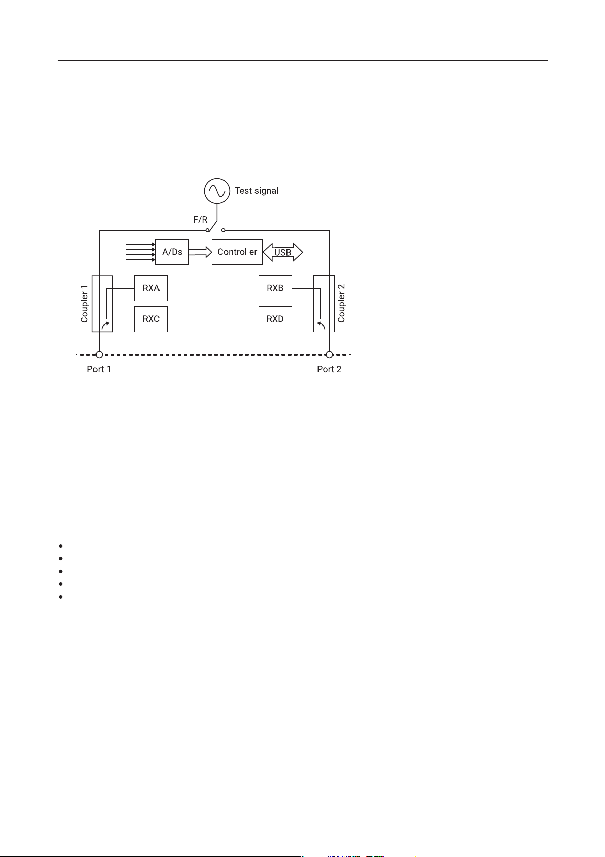
3 Description

The PicoVNA 106 is a PC-driven vector network analyzer capable of operation over the range of 300 kHz to 6 GHz. It can perform direct measurements of forward and reverse parameters with up to 118 dB of dynamic range. The test frequency can be set with a resolution of 10 Hz or less. A simplified block diagram of the instrument is shown below:

Simplified block diagram of the PicoVNA 106

The architecture is based on a four-receiver ("Quad RX") arrangement using a bandwidth of up to 140 kHz. Couplers 1 and 2 are wideband RF bridge components which provide the necessary directivity in both directions. Signal detection is by means of analog-to-digital converters used to sample the IF signal. The sample data is processed by the embedded controller to yield the I and Q components. The detection system operates with an IF of 1.3 MHz and employs a patented circuit technique to yield fast speeds with very low trace noise.

The instrument's software runs on a personal computer and communication with the instrument is through the USB interface. The software carries out the mathematical processing and allows the display of measured parameters in many forms, including:

frequency domain time domain de-embedding utility measuring output power at the 1 dB gain compression point measuring AM to PM conversion

PicoVNA 106 6 GHz Vector Network Analyzer 9

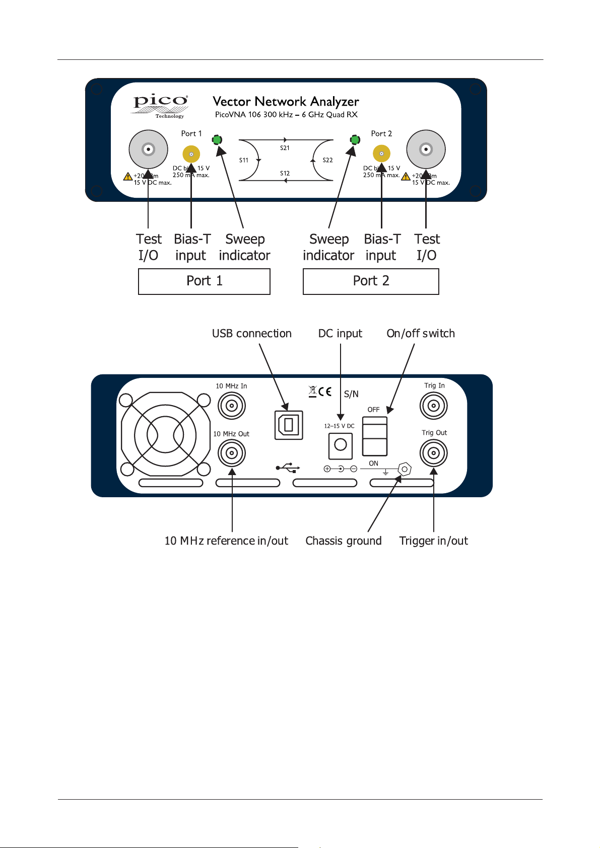
Front panel of the PicoVNA 106

Back panel of the PicoVNA 106

Vector network analyzer basics10

4 Vector network analyzer basics

4.1 Introduction

A vector network analyzer is used to measure the performance of circuits or networks such as amplifiers, filters, attenuators, cables and antennas. It does this by applying a test signal to the network to be tested, measuring the reflected and transmitted signals and comparing them to the test signal. The vector network analyzer measures both the magnitude and phase of these signals.

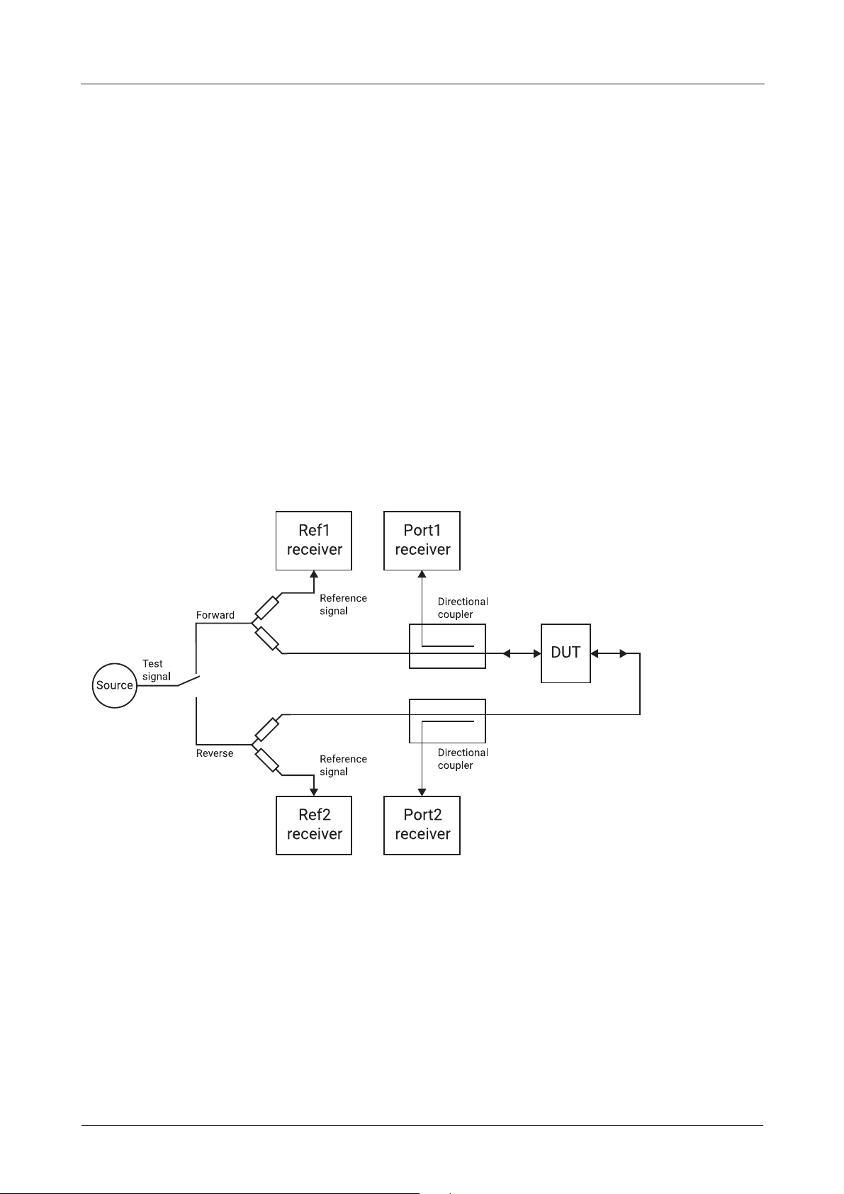
4.2 Structure of the VNA

The VNA consists of a tunable RF source, the output of which is split into two paths. The signal feeds to the couplers are each measured by their respective reference receivers through power dividers. In the forward mode, the test signal is passed through a directional coupler or directional bridge before being applied to the DUT. The directional output of the coupler, which selects only signals reflected from the input of the DUT, is connected to the Port1 receiver where the signal’s magnitude and phase are measured. The rest of the signal, the portion that is not reflected from the input, passes through the DUT to the Port2 receiver where its magnitude and phase are measured. The measurements at the Port1 and Port2 receivers are referenced to the measurements made by the Ref1 and Ref2 receivers so that any variations due to the source are removed. The Ref1 and Ref2 receivers also provide a reference for the measurement of phase.

Simplified vector network analyzer block diagram

In reverse mode, the test signal is applied to the output of the DUT, and the Port2 receiver is used to measure the reflection from the output port of the DUT while the Port1 receiver measures the reverse transmission through the DUT.

PicoVNA 106 6 GHz Vector Network Analyzer 11

4.3 Measurement

Vector network analyzers have the capability to measure phase as well as magnitude. This is important for fully characterizing a device or network either for verifying performance or for generating models for design and simulation. Knowledge of the phase of the reflection coefficient is particularly important for matching systems for maximum power transfer. For complex impedances the maximum power is transferred when the load impedance is the complex conjugate of the source impedance (see figure).

Matching a load for maximum power transfer

Measurement of phase in resonators and other components is important in designing oscillators. In feedback oscillators, oscillation occurs when the phase shift round the loop is a multiple of 360° and the gain is unity. It is important that these loop conditions are met as close as possible to the center frequency of the resonant element to ensure stable oscillation and good phase noise performance.

The ability to measure phase is also important for determining phase distortion in a network. Phase distortion can be important in both analog and digital systems. In digital transmission systems, where the constellation depends on both amplitude and phase, any distortion of phase can have serious effects on the errors detected.

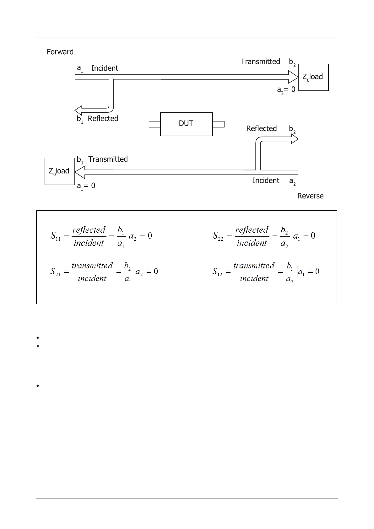
4.4 S-parameters

The basic measurements made by the vector network analyzer are S (scattering) parameters. Other parameters such as H, Y and Z parameters may all be deduced from the S-parameters if required. The reason for measuring S-parameters is that they are made under conditions that are easy to produce at RF. Other parameters require the measurement of currents and voltages, which is difficult at high frequencies. They may also require open circuits or short circuits that can be difficult to achieve at high frequencies, and may also be damaging to the device under test or may cause oscillation.

Forward S-parameters are determined by measuring the magnitude and phase of the incident, reflected and transmitted signals with the output terminated with a load that is equal to the characteristic impedance of the test system (see figure below).

Vector network analyzer basics12

S-parameters definition

The measured parameters are presented in a file similar to the one below. The format is as follows:

Header lines: these start with a ! symbol and give general information such as time and date. Format line: this starts with a # symbol and gives information about the format of the data.

o First field gives the frequency units, in this case MHz o Second field indicates the parameters measured, in this case S-parameters o Third field indicates the format of the measurement, in this case MA meaning magnitude and angle.

Others formats are RI, meaning real and imaginary, and DB, meaning log magnitude and angle. Data lines. The number of columns of data depends on the parameters that have been measured. o A 1-port measurement measures the reflected signal from the device under test and usually produces

three columns. If the format is MA (magnitude and angle), the first column is the measurement

frequency, the second is the magnitude of S

second column is the real part of S

and the third column is the imaginary part of S11.

and the third is the angle of S11. If the format is RI, the

o When a reflection and transmission measurement is made there are five columns of data. Column 1

is the measurement frequency, columns 2 and 3 contain S

imaginary data, and columns 4 and 5 contain S

magnitude and angle or real and imaginary data.

magnitude and angle or real and

o If a full 2-port measurement is made, there will be nine columns of data. Column 1 contains frequency

information, columns 2 and 3 S

data, 4 and 5 S21 data, 6 and 7 S12 data, and 8 and 9 S22 data.

PicoVNA 106 6 GHz Vector Network Analyzer 13

The PicoVNA 106 can generate full set of 2-port parameters but you can choose to export either 1-port .s1p or full 2-port .s2p S-parameter files to suit most RF and microwave circuit simulators.

Part of a typical 2-port S-parameter file is shown below. The header shows that the frequency units are MHz, the data format is Magnitude and Angle and the system impedance is 50 Ω. Column 1 shows frequency, 2 and 3 S

! 06/09/2005 15:47:34 ! Ref Plane: 0.000 mm # MHZ S MA R 50 ! 3 0.00776 16.96 0.99337 -3.56 0.99324 -3.53 0.00768 12.97

17.985 0.01447 19.99 0.9892 -20.80 0.98985 -20.72 0.01519 15.23

32.97 0.01595 20.45 0.98614 -37.96 0.98657 -37.95 0.01704 6.40

47.955 0.01955 28.95 0.98309 -55.15 0.98337 -55.10 0.018 1.75

62.94 0.02775 24.98 0.98058 -72.29 0.98096 -72.29 0.0199 -6.07

77.925 0.03666 11.76 0.97874 -89.46 0.9803 -89.45 0.02169 -23.06

92.91 0.04159 -6.32 0.97748 -106.62 0.9786 -106.62 0.01981 -48.43

107.895 0.0426 -24.79 0.97492 -123.77 0.97579 -123.89 0.01424 -87.79

122.88 0.0396 -41.35 0.97265 -141.25 0.97269 -141.30 0.00997 -166.81

137.865 0.03451 -52.96 0.96988 -158.65 0.96994 -158.76 0.01877 113.15

152.85 0.03134 -56.07 0.96825 -176.27 0.96858 -176.28 0.03353 69.81

167.835 0.03451 -57.72 0.96686 166.10 0.96612 165.99 0.04901 34.83

182.82 0.04435 -67.59 0.9639 148.18 0.96361 148.21 0.06131 1.42

197.805 0.05636 -86.28 0.96186 130.15 0.96153 130.06 0.07102 -33.33

212.79 0.06878 -110.45 0.95978 111.82 0.95996 111.90 0.07736 -69.57

227.775 0.08035 -136.14 0.9557 93.50 0.9568 93.41 0.08303 -107.21

242.76 0.09099 -161.24 0.95229 74.84 0.95274 74.89 0.08943 -144.34

257.745 0.10183 175.34 0.94707 56.03 0.94755 55.95 0.09906 -179.63

, 4 and 5 S21, 6 and 7 S12, and 8 and 9 S22.

Vector network analyzer basics14

4.5 Displaying measurements

Input and output parameters, S11 and S22, are often displayed on a polar plot or a Smith chart. The polar plot shows the result in terms of the complex reflection coefficient, but impedance cannot be directly read off

the chart. The Smith chart maps the complex impedance plane onto a polar plot. All values of reactance and all positive values of resistance, from 0 to ∞, fall within the outer circle. This has the advantage that impedance values can be read directly from the chart.

The Smith chart

4.6 Calibration and error correction

Before accurate measurements can be made, the network analyzer needs to be calibrated. In the calibration process, well-defined standards are measured and the results of these measurements are used to correct for imperfections in the hardware. The most common calibration method, SOLT (short, open, load, through), uses four known standards: a short circuit, an open circuit, a load matched to the system impedance, and a through line. These standards are usually contained in a calibration kit and their characteristics are stored on the controlling PC in a Cal Kit definition file. Analyzers such as the PicoVNA 106 that have a full Sparameter test set can measure and correct all 12 systematic error terms.

PicoVNA 106 6 GHz Vector Network Analyzer 15

(

Six key sources of errors in forward measurement.

Another six sources exist in the reverse measurement

not shown).

4.7 Other measurements

S-parameters are the fundamental measurement performed by the network analyzer, but many other parameters may be derived from these including H, Y and Z parameters.

4.7.1 Reflection parameters

The input reflection coefficient Γ can be obtained directly from S11:

ρ is the magnitude of the reflection coefficient i.e. the magnitude of S

ρ = |S11|

Sometimes ρ is expressed in logarithmic terms as return loss:

return loss = –20 log(ρ)

VSWR can also be derived:

VSWR definition

11:

4.7.2 Transmission parameters

Transmission coefficient T is defined as the transmitted voltage divided by the incident voltage. This is the same as S

Vector network analyzer basics16

If T is less than 1, there is loss in the DUT, which is usually referred to as insertion loss and expressed in decibels. A negative sign is included in the equation so that the insertion loss is quoted as a positive value:

If T is greater than 1, the DUT has gain, which is also normally expressed in decibels:

4.7.3 Phase

The phase behavior of networks can be very important, especially in digital transmission systems. The raw phase measurement is not always easy to interpret as it has a linear phase increment superimposed on it due to the electrical length of the DUT. Using the reference plane function the electrical length of the DUT can be removed leaving the residual phase characteristics of the device.

Operation on phase data to yield underlying characteristics

4.7.4 Group delay

Another useful measurement of phase is group delay. Group delay is a measure of the time it takes a signal to pass through a network versus frequency. It is calculated by differentiating the phase response of the device with respect to frequency, i.e. the rate of change of phase with frequency:

The linear portion of phase is converted to a constant value typically, though not always, representing the average time for a signal to transit the device. Differences from the constant value represent deviations from linear phase. Variations in group delay will cause phase distortion as a signal passes through the circuit.

When measuring group delay the aperture must be specified. Aperture is the frequency step size used in the differentiation. A small aperture will give more resolution but the displayed trace will be noisy. A larger aperture effectively averages the noise but reduces the resolution.

PicoVNA 106 6 GHz Vector Network Analyzer 17

4.7.5 Gain compression

The 1 dB gain compression point of amplifiers and other active devices can be measured using the power sweep. The small signal gain of the amplifier is determined at low input power, then the power is increased and the point at which the gain has fallen by 1 dB is noted.

The 1 dB gain compression is often used to quote output power capability

4.7.6 AM to PM conversion

Another parameter that can be measured with the VNA is AM to PM conversion. This is a form of signal distortion where fluctuations in the amplitude of a signal produce corresponding fluctuations in the phase of the signal. This type of distortion can have serious effects in digital modulation schemes where both amplitude and phase accuracy are important. Errors in either phase or amplitude cause errors in the constellation diagram.

4.7.7 Time domain reflectometry (TDR)

Time domain reflectometry is a useful technique for measuring the impedance of transmission lines and for determining the position of any discontinuities due to connectors or damage. The network analyzer can determine the time domain response to a step input from a broad band frequency sweep at harmonically related frequencies. An inverse Fourier Transform is performed on the reflected frequency data (S

the impulse response in the time domain. The impulse response is then integrated to give the step response. Reflected components of the step excitation show the type of discontinuity and the distance from the calibration plane.

A similar technique is used to derive a TDT (Time Domain Transmission) signal from the transmitted signal data (S

provides a more detailed treatment of TDR and TDT.

). This can be used to measure the rise time of amplifiers, filters and other networks. The following

) to give

Vector network analyzer basics18

4.7.7.1 Traditional TDR

The traditional TDR consists of a step source and sampling oscilloscope (see figure below). A step signal is generated and applied to a load. Depending on the value of the load, some of the signal may be reflected back to the source. The signals are measured in the time domain by the sampling scope. By measuring the ratio of the input voltage to the reflected voltage, the impedance of the load can be determined. Also, by observing the position in time when the reflections arrive, it is possible to determine the distance to impedance discontinuities.

Traditional TDR setup

4.7.7.1.1 Example: shorted 50 ohm transmission line

Simplified representation of the response of a shorted line.

PicoVNA 106 6 GHz Vector Network Analyzer 19

For a transmission line with a short circuit (figure above) the incident signal sees the characteristic impedance of the line so the scope measures Ei. The incident signal travels along the line to the short circuit where it is reflected back 180° out of phase. This reflected wave travels back along the line canceling out the incident wave until it is terminated by the impedance of the source. When the reflected signal reaches the scope the signal measured by the scope goes to zero as the incident wave has been canceled by the reflection. The result measured by the scope is a pulse of magnitude Ei and duration that corresponds to the time it takes the signal to pass down the line to the short and back again. If the velocity of the signal is known, the length of the line can be calculated:

where v is the velocity of the signal in the transmission line, t is the measured pulse width and d is the length of the transmission line.

4.7.7.1.2 Example: open-circuited 50 ohm transmission line

Simplified representation of the response of a open line

In the case of the open circuit transmission line (figure above) the reflected signal is in phase with the incident signal, so the reflected signal combines with the incident signal to produce an output at the scope that is twice the incident signal. Again, the distance d can be calculated if the velocity of the signal is known.

4.7.7.1.3 Example: resistively terminated 50 ohm transmission line

Simplified representation of the response of a resistively terminated line

Vector network analyzer basics20

4.7.7.1.4 Reactive terminations and discontinuities

Reactive elements can also be determined by their response. Inductive terminations produce a positive pulse. Capacitive terminations produce a negative pulse.

Simplified representation of the response of a reactively terminated line

Similarly, the position and type of discontinuity in a cable, due to connectors or damage, can be determined. A positive pulse indicates a connector that is inductive or damage to a cable, such as a removal of part of the outer screen. A negative-going pulse indicates a connector with too much capacitance or damage to the cable, such as being crushed.

Simplified representation of the response of a line discontinuity

4.7.7.2 Time domain from frequency domain

An alternative to traditional TDR is where the time domain response is determined from the frequency domain using an Inverse Fast Fourier Transform (IFFT). Several methods are available for extracting time domain information from the frequency domain. The main methods are lowpass and bandpass.

4.7.7.2.1 Lowpass method

The lowpass method can produce results that are similar to the traditional TDR measurements made with a time domain reflectometer using a step signal, and can also compute the response to an impulse. It provides both magnitude and phase information and gives the best time resolution. However, it requires that the circuit is DC-coupled. This is the method supported by the PicoVNA 106.

The lowpass method uses an Inverse Fourier Transform to determine the impulse response in the time domain from the reflection coefficient measured in the frequency domain. The DC component is extrapolated from the low-frequency data to provide a phase reference. Alternatively, if the DC termination is known it can be entered manually. Once the impulse response is computed, the step response may be determined from the time integral of the impulse response. In the step response mode the trace is similar to that of a TDR, except that there is no step at t = 0. When the time domain response is derived from the frequency information the value at t = 0 is the impedance of the transmission line or load immediately following the calibration plane. The value is referenced to 50 Ω, the characteristic impedance of the system. For example, an open circuit would appear as a value of +1 unit relative to the reference value and a short circuit would appear as a value of –1 unit relative to the reference value (see example TDR plots above).

PicoVNA 106 6 GHz Vector Network Analyzer 21

To facilitate the use of the Inverse Fourier Transform to compute the time domain response, the samples in the frequency domain must be harmonically related and consist of 2 in the PicoVNA 106 makes available special 512, 1024, 2048 and 4096-frequency-point calibrations with a stop frequency of up to 6000 MHz. The resulting alias-free range is a function of the number of frequency points (N) and the total frequency span. It is given by the expression:

So, the available ranges on the PicoVNA 106 are approximately 100 ns, 171 ns, 341 ns and 683 ns.

The transform returns twice the number of points of the calibration in the time domain. Therefore the above ranges provide time resolutions of approximately 98ps to 84ps.

points. For this reason, the TDR facility

4.7.7.2.2 Bandpass method

The bandpass method provides only magnitude information so it is not possible to distinguish between inductive and capacitive reactances. Also, the time resolution is only half as good as in the lowpass mode. However, the method can be used for circuits where there is no DC path and hence is suitable for ACcoupled circuits such as bandpass filters. This method is not currently supported by the PicoVNA 106.

4.7.7.3 Windowing

The bandwidth of the network analyzer is limited by the frequency range, so the frequency domain data will be truncated at the bandwidth of the analyzer. Also the analyzer gathers data at discrete frequencies. The result of the sampled nature of the data and the truncation in the frequency domain is to produce a sin(x)/x response when transformed to the time domain. This appears as ringing on both the displayed impulse response and the step response. To overcome this problem, a technique known as windowing can be applied to the frequency domain data before implementing the Inverse Fourier Transform.

The windowing function progressively reduces the data values to zero as the edge of the frequency band is approached, thus minimizing the effect of the discontinuities. When the modified data is transformed, the ringing is reduced or removed depending on the selected windowing function. However, the windowing function reduces the bandwidth and so increases the width of the pulse in impulse response mode and slows the edge in step response mode. A balance must be made between the width of the pulse, or speed of the edge, and the amount of ringing to be able to determine closely spaced discontinuities. The PicoVNA 106 allows you to choose a rectangular window (no bandwidth reduction), a Hanning window (raised cosine), or a Kaiser–Bessel window. The order of the Kaiser–Bessel window is configurable.

4.7.7.4 Aliasing

The sampled nature of the data means it is subject to the effects of aliasing. The result is repetition of timedomain response at the effective sampling rate in the frequency domain. This limits the maximum time delay and hence maximum cable length that can be observed. In the PicoVNA 106 this is 683ns (approximately 138m of cable).

Getting started22

5 Getting started

Refer to the Quick Start Guide above for initial instructions, then return here for more detail.

5.1 Minimum requirements

The recommended minimum requirements to operate the VNA are as follows.

PC or laptop Pentium 4 (2 GHz) or equivalent 2 GB of RAM 200 MB of hard disk storage available on the C: partition Windows 7, 8 or 10 Minimum display resolution of 1280 x 720 USB port

The performance of the software is influenced by the performance of the PC and video adaptor installed in it. It is important that an adaptor with good graphics performance is used. As a general guide, it is recommended that an adaptor with at least 64 MB of memory is used.

5.2 Software installation

Follow the Quick Start Guide to install the software from the disk or from www.picotech.com. The installer will copy the program and the USB driver to your computer. You need administrative privileges in order to run the installer.

The installer creates a support directory at C:\User\Public\Documents\PicoVNA2. This directory contains the following files:

xxx-log.txt The status log file. ‘xxx’ is the serial number DefCal.cal Default calibration data (last used calibration) UsersGuide.pdf This User's Guide Support\ Folder with data files to support the software

5.2.1 Typical error messages

On Windows 7 machines it is common to see the following error message:

It is safe to click Ignore to continue the installation.

PicoVNA 106 6 GHz Vector Network Analyzer 23

5.3 Switching on the VNA

When the VNA is powered on, the front-panel channel activity indicators will flash to indicate that the controller has started correctly.

5.4 Calibration kit parameters

The minimum requirements to carry out a 12-term calibration (full error correction) depend on the device to be tested. For example, the most accurate calibration is for ‘insertable’ devices, and this requires a total of six standards: three of the four in each of the male and female cal standards.

An ‘insertable’ device is one that has connectors of different sexes at its ports. On the other hand, a calibration for a non-insertable device can be carried out using only three standards by using the “unknown through” calibration method.

The calibration kits parameters can be inspected using the Calibration Kit Parameters window (see below) found under the Tools menu. From this the kit editor can be launched to modify and create new kits as discussed later in the section.

The ‘unknown thru’ calibration method only requires that the ‘thru’ adaptor be reciprocal: that is, have S

Calibration Kit window. The short/open offsets are in mm in air.

Getting started24

5.4.1 Insertable DUT

Open circuit (2 pieces, one male and one female) Short circuit (2 pieces, one male and one female) Matched termination (2 pieces, one male and one female) Through connection test cable(s)

For insertable DUTs the requirement is for two calibration kits, one of each sex. Generally, it is required that the matched termination should be of good quality and, as a guide, should have a return loss of better than 40 dB. However, the PicoVNA 106 allows terminations with relatively poor return loss values to be used and still maintain good accuracy. This is discussed in Using a matched termination

5.4.2 Non-insertable DUT

Open circuit (1 piece) Short circuit (1 piece) Matched termination (1 piece) Either a characterized through connection adaptor (1 piece) or any uncharacterized reciprocal adaptor Through connection test cable(s)

For non-insertable DUTs only a single calibration kit is required. In addition, a reciprocal but otherwise unknown through adaptor, or a fully characterized through adaptor, is required. These are supplied with all Pico standard kits.

5.4.3 Open circuit model

The open circuit capacitance model used is described by the equation below, where Freq is the operating frequency. Generally, with typical open circuit standards, the effect is small, amounting to no more than a few degrees of phase shift at 6 GHz.

= C0 + C1Freq + C2Freq2 + C3Freq

open

In addition, an offset length (sometimes referred to as offset delay) can be entered as well as the loss of the offset line.

5.4.4 Short circuit model

The short circuit inductance is modeled by an inductance component and in addition, a non-zero offset length can be entered together with the loss of the offset line.

5.4.5 Short and open without models

The PicoVNA 106 supports short and open standards defined by data only. In this case the data is supplied in the form of a 201-frequency-points table. Each frequency point has three comma-separated entries: frequency (in MHz), real part of the reflection coefficient and the imaginary part of the reflection coefficient.

5.4.6 Calibration kit editor

As already mentioned, the calibration kit editor can be used to create or edit an existing calibration kit. The figure below shows the editor window. A typical example is to create a new kit using an existing kit as a template to speed the process. So, the process would be to first load the existing calibration kit from the

Calibration Kit Parameters

required. Finally, click Save Kit to save the new kit under a new name.

window. Type the new kit name in the name box and modify the parameters as

PicoVNA 106 6 GHz Vector Network Analyzer 25

In the above example, if the existing kit loaded had load data or through data and you want to replace this with new data, uncheck the appropriate box and then re-check it.

Calibration Kit Editor

The calibration kits optionally supplied with the PicoVNA 106 provide an economical solution while retaining good measurement accuracy. They are supplied with SMA or precision PC3.5 (SMA-compatible) connectors. Refer to the PicoVNA 106 Data Sheet for details.

5.4.7 Using a matched termination with poor return loss or unmodeled short and open

A successful calibration can be carried out without the need for a good-quality matched load. In order to retain accuracy, it is necessary to provide the instrument with accurate performance data of the matched load to be used. The data needs to be in a fixed format thus:

Frequency (MHz)

1.0 -1.7265E-03 7.7777E-05

30.995 -1.6588E-03 3.3093E-04

60.99 -1.4761E-03 5.9003E-04

90.985 -1.4653E-03 1.0253E-03

120.98 -1.3841E-03 1.2608E-03

150.975 -1.1924E-03 1.5800E-03

240.96 -1.0884E-03 1.9085E-03

300.95 -8.7216E-04 2.1355E-03

330.945 -7.0326E-04 2.4109E-03

360.94 -5.7006E-04 2.6790E-03

S11 (real)

S11 (imaginary)

There must be 201 data lines. Typically these should cover the band 1MHz to 6.00GHz. No empty or

comment lines are allowed.

Table: format for characteristics of matched load

In the case when the models for the open and short are not known, it is possible to enter measured data in the same format as shown above. This approach can give good results if the open and short can be measured accurately, particularly at the higher frequencies where it is usually difficult to model components accurately.

When supplied, the data for the through connection adaptor must be in the format shown below. The data must be a full set of S-parameters with no empty or comment lines. It is recommended that the data spans the full frequency range from 1 MHz to 6000 MHz.

Getting started26

Freq (MHz) S11r S11i S21r S21i S12r S12i S22r S22i

0.3 1.1450E-04 -1.0852E-04 0.9965E-01 -1.0394E-03 9.9947E-01 -7.4717E-04 1.0723E-04 4.9711E-05

40.3 2.9307E-04 1.9923E-04 9.9973E-01 -1.0241E-02 9.9934E-01 -1.0505E-02 2.0715E-04 2.0814E-04

80.3 4.1774E-04 4.3168E-04 9.9922E-01 -1.9672E-02 9.9927E-01 -1.9668E-02 2.8195E-04 2.8897E-04

120.3 5.3415E-04 5.7609E-04 9.9898E-01 -2.9165E-02 9.9855E-01 -2.8852E-02 4.0525E-04 2.8043E-04

160.3 7.1924E-04 6.4942E-04 9.9883E-01 -2.9165E-02 9.9855E-01 -2.8852E-02 4.0646E-04 2.8133E-04

200.3 7.8941E-04 7.5903E-04 9.9834E-01 -3.8214E-02 9.9846E-01 -3.8128E-02 5.4323E-04 2.2344E-04

240.3 9.9069E-04 7.8162E-04 9.9792E-01 -5.7033E-02 9.9758E-01 -4.7805E-02 5.7273E-04 2.9411E-04

280.3 1.0791E-03 8.0397E-04 9.9715E-01 -6.6419E-02 9.9699E-01 -6.5967E-02 5.7191E-04 2.6551E-04

320.3 1.2779E-03 8.5429E-04 9.9648E-01 -7.5557E-02 9.9625E-01 -7.5449E-02 6.3081E-04 2.9580E-04 ...

and so on, to a total of 201 frequency points

Table: Format for the characteristics of the through connector. These must be a full set of S-parameters

(real and imaginary).

To add matched load, short and open, or through adaptor data to a calibration kit, follow the steps below:

Load kit using the Kit Editor (see Calibration Kit) Check the Load Data Available box and similarly the boxes for the Thru and Short and Open circuits in the Kit Editor parameters window. If the existing kit already has load, short and open, or through data, uncheck and recheck the appropriate box. If this is not done, the existing data will be kept and copied to the new kit. If needed, manually enter the rest of the kit parameters. Ensure that the correct offset is entered. Click Save Kit When prompted, select the data file containing the matched load or the through adaptor data in the format shown above. Save the kit for future use by clicking the Save Kit button (see Calibration Kit).

Note: When a kit is loaded, any available matched load or through adaptor data that is associated with the kit will be automatically loaded.

The calibration kits available for the PicoVNA 106 come complete with matched load, short and open, and through adaptor data. Copy these files to your computer for easy access.

It is critically important that the correct kit data, with the correct serial number, is loaded.

PicoVNA 106 6 GHz Vector Network Analyzer 27

6 Operation

The PicoVNA 2 software allows you to program the measurement parameters and plots the measurement results in real time. The main window includes a status panel that displays information including calibration status, frequency sweep step size and sweep status. The Help menu includes a copy of this manual.

6.1 The PicoVNA 2 main window

The PicoVNA 2 main window is shown below. It is dominated by a large graphics area where the measurement results are plotted together with the readout of the markers. One, two or four plots can be displayed simultaneously. The plots can be configured to display the desired measurements.

User interface window

6.1.1 Display setup

Setting up the display is carried out through the Display Set Up window which is called up from the main window by clicking Display. The window is shown below. The typical sequence to set up the display is as follows:

Set the number of channels to be displayed by clicking the appropriate radio button under Display

Channels

Select the desired active channel from the drop-down list (can also be selected by clicking on a marker in the main window on the desired display channel)

Operation28

Select the channel to set up by clicking the appropriate radio button under Select Choose the desired parameter to display on this channel from the drop-down list under Parameter / Graph

Type

Choose the desired graph type from the drop-down list under Parameter / Graph Type Select the vertical axis values from the Vertical Axis section. Optionally, click Autoscale to automatically set the sensitivity and reference values. Note that reference position 1 is at the top (see second figure below). Click Apply to apply the selected values Repeat the above steps for each display needed

Note: The Active Channel must be one of the displayed channels.

The Display Set Up window is used to set up the measurements displa

Display graph parameters

PicoVNA 106 6 GHz Vector Network Analyzer 29

The colors of the main graphics display can be changed to suit individual preferences. This can be done by selecting the Color Scheme item from the Tools menu. To set a color, click the color preview box next to the item name.

Once you have set up a color scheme, you can save and recall it as a Cal and Status setting using the File menu.

Editing graph parameters using the mouse

The figure above shows how the mouse can be used to quickly adjust reference position, reference value and vertical scale sensitivity.for the graph. Drag the indicated values up and down to adjust, or type a new value where the cursor indicates.

6.1.2 Data markers

It is possible to display up to eight markers on each display. They are set up by clicking on the Markers button (see figure below). There are four possible marker modes as follows:

Active marker: The active marker is the marker used for comparison when the delta marker mode (switched on by selecting a reference marker) is on. One of the displayed markers must be chosen as the active marker.

Reference marker: The reference marker causes the delta marker mode to be switched on. The value difference between the active marker and the reference markers is shown on the right hand marker display panel.

Fixed marker: A fixed marker cannot be moved and its position is not updated with subsequent measurement values. It provide a fixed reference point. Only a reference marker can be made a fixed marker. Once a marker is fixed, it cannot be moved until it is unfixed.

Normal marker: The value of a normal marker is displayed on the right-hand marker readout panel and in lower resolution readouts below each measurement plot.

Any marker (except a fixed marker) can be moved to a new position by left clicking on it (on any displayed channel) and dragging it to a new position.

Operation30

The markers set up form provides a Peak / Minimum Search facility. This places marker 1 at either the peak or minimum value on the displayed trace on the active channel when the corresponding Find button is pressed.

The Markers Set Up dialog is used to display measurement markers

PicoVNA 106 6 GHz Vector Network Analyzer 31

Change the marker type by right-clicking on any marker on the active channel. Note that only the reference

marker can be fixed.

The peak / minimum search facility provides a means of placing additional markers to indicate the 3 or 6 dB bandwidth. If either the 3 dB or 6 dB band box are selected, then clicking Find will place markers 2 and 3 on the frequency points either side of marker 1 which are 3 dB or 6 dB relative to it. Note that for best accuracy a sufficient number of sweep points should be used. This will ensure a fine enough resolution to allow accurate determination of the band points.

6.1.3 Measurement enhancement

The measurement enhancement options are displayed (see figure below) by clicking Enhancement in the main UI window. The options available are as follows.

Averages (1 to 255, on a point by point basis) Trace Smoothing (0 to 10%) Bandwidth (140 kHz to 10 Hz) Port 1 Level (+6 dBm to –20 dBm, 0.1 dB resolution) CW sweep time per point (500 to 65 000 μs/point) Reference Plane Extension (manual entry or automatic) Effective dielectric constant of device under test (manual entry to correct plane extension values) De-embedding (specify embedding networks at ports 1 and or 2)

Impedance conversion for devices that are not 50 Ω

Operation32

The measurement enhancement window

The Bandwidth setting refers to the receiver bandwidth. Maximum sweep speed is achieved with the highest (140 kHz) setting. On the other hand, the widest dynamic range (lowest noise floor) is achieved with the lowest value, 10 Hz. Note that the bandwidth setting used during calibration determines the maximum dynamic range achievable during measurements. So, consider this when carrying out a calibration. For example, if you need to carry out measurement over more than, say 90 dB dynamic range, then use a 500 Hz or less bandwidth setting when calibrating.

The Port 1 Level sets the test signal level. The default value is +3 dBm as this gives best overall measurement accuracy. However, it may be necessary, particularly when measuring active devices (e.g. amplifiers) to reduce the test level. For maximum dynamic range, then use the highest power setting. For best measurement accuracy it is recommended that the calibration is carried out at the same test level as it is intended to use for the measurement. Whenever the test level is different to that used for the calibration, a ‘?’ will be added to the calibration status indicator on the Status Panel (Fig. 6.1)

The Reference Plane facility allows the reference plane of each parameter measurement to be arbitrarily moved away from the calibration plane. The value entered applies to the measurement parameter (S

or S22) displayed on the active channel. Note that the same plane value will be used for all other

, S21,

measurements on that same parameter regardless if they are on the active channel or not.

The Auto Reference automatically moves the reference plane. It uses the measurement on the active channel. This feature is particularly useful, for example, when measuring microstrip devices and it is necessary to remove the effect of the connecting input and output lines. It takes the effective dielectic constant value entered to correct the displayed value. Refer to Reference plane extension and de-embedding for more details.

Note: The reference plane must be at 0 mm for the Auto Ref function to work correctly. Also, Enhancement window changes only take place when the instrument is sweeping.

PicoVNA 106 6 GHz Vector Network Analyzer 33

The Effective Dielectric of the device under test can be entered so that the displayed Reference Plane extension values (shown on the Enhancement Window) are corrected accordingly when the Auto Ref button is clicked. The default value is 1.0 and the maximum value allowed is 50.0.

Note: The reference plane extension value shown in the main window

on the markers display panel on the

right is the reference plane extension as shown in the Enhancement window.

The de-embedding facility is explained in detail in Reference plane extension and de-embedding.

The System Z

Conversion facility allows measurements, which are always taken in 50 Ω, to be converted to

another impedance selected by the user. This feature can be useful, for example, for measuring 75 Ω devices. The value of Z

entered must be real (purely resistive) and must be within the range of 10 Ω to 200

Ω. Whenever this facility is selected, an indicator is displayed on the top right corner of the graphics display as shown in the second figure below. Note that when requested, impedance conversion will performed on the live measurement and any stored memory trace.

There are two possible ways of using the System Z

Conversion facility. For example, 75 Ω devices can be

measured using the techniques illustrated below.

Possible techniques for measuring 75 Ω devices.

Impedance matching pads can be used to measure a connectorized device.

A discrete device mounted on a 50 Ω test jig is somewhat simpler to measure.

The steps necessary for each of the two techniques illustrated in the figure above are as follows:

75 Ω device with connectors

i. Connect 50 Ω to 75 Ω impedance matching networks (e.g. matching pads) at the ends of the cables

connected to ports 1 and 2. ii. In the Enhancement window, check the Convert System Zo box iii. Check External Zo match to indicate external matching networks in use iv. Enter 75 in the Convert System Zo value box and click Apply v. Proceed to calibrate using a 75 Ω calibration kit vi. Connect the DUT and start the measurement

75 Ω device mounted on 50 Ω test jig

i. In the Enhancement window, uncheck the Convert System Zo box ii. Calibrate at the ends of the test cables using a 50 Ω calibration kit iii. Apply de-embedding to remove test jig effects. See Calibration kit

for some suggestions.

iv. In the Enhancement window, check the Convert System Zo box

Operation34

v. Uncheck the External Zo match box (in this case mathematical impedance conversion is done by the

software) vi. Enter 75 in the Convert System Zo value box and click Apply vii. Connect the DUT and start the measurement

System impedance chosen is displayed on the top right corner

Note: S-parameters are interrelated, so, when using the Z matching networks) without a full set of S-parameters available (e.g. only an S

conversion facility (and no external impedance

calibration) the program

will assume values for the unavailable parameters as shown in the following table. A warning will be displayed in such cases.

10–6, j0.0 10–6, j0.0 10–6, j0.0 10–6, j0.0

Table: Values assumed for parameters not available during Z0 conversion

6.1.4 Memory facility

The current displayed data on each channel can be stored in memory. Also, each channel can be stored independently of all others. The Memory Set Up window is used to store the data and this window can be displayed by clicking Memory in the main window.

The Memory Set Up window is used to store data into memor

Once the data is stored, it can be displayed by clicking Display Data and Memory in the main window.

There are three vector math functions available: sum, subtraction and division. The selected function is used when you select the Display Memory Math function on the main window.

PicoVNA 106 6 GHz Vector Network Analyzer 35

The trace hold is used to store the maximum or minimum values on the memory trace. Trace hold is not available when group delay is displayed.

6.1.5 Limit lines facility

The limit lines facility allows six segments to be defined for each displayed graph. By taking advantage of the overlapping capability (see below) a maximum of 11 segments can be created The set up window, shown below, is displayed by clicking Limit Lines in the main window.

Overlapping segments

All valid segments entered are loaded in sequence (i.e. segment 1 first) with the each segment loaded having priority over the previous segment. This feature allows overlapping segments to be loaded. For example, if segment 1 is specified to cover, say, 400 to 800 MHz, then a second segment can be specified to a section of this band, for example, 500 to 600 MHz. This would result in a total of three segments—that is, 400 to 500, 500 to 600 and 600 to 800 MHz—even though only two were specified. An example of a complex 11-segment template is shown in the first plot below.

Alarm

An alarm facility is provided with the limit lines. This provides audible warning during a sweep if any measurement exceeds the limits set. A visible indication of the last measurement and measurement channel in error is provided on the status panel where normally the calibration type is displayed. In addition a symbol is drawn on the trace indicating the last error point detected as shown in the second plot below. The alarm is available for all graph types except Smith plots.

The Limit Lines Set Up allows at least six segments per graph

Complex Limit Lines templates are possible by overlapping segments

Operation36

Limit Lines failure graphical visual indicator

6.1.6 Status panel

The status panel in the main window provides useful information as follows:

Instrument serial number

Calibration status (S11, S21, S11 + S21, 12 terms or U/T). A question mark indicates that the test power has

been changed from that used for calibration

Test signal power. This is the Port 1 signal level

Sweep status. Indicates whether instrument is sweeping

Frequency step. Step size of sweep

Sweep points. Number of points in programmed sweep.

Limit Lines alarm if any measurement exceed the set limits (temporarily replaces Calibration status)

PicoVNA 106 6 GHz Vector Network Analyzer 37

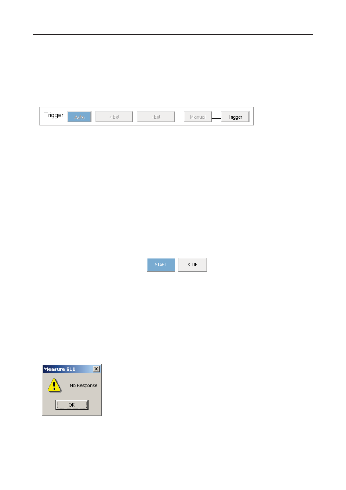
6.1.7 Triggered sweep

It is possible to synchronize each measurement sweep to an external trigger. Simply click the appropriate radio button in the main window and ensure that a trigger signal is connected to the instrument’s rear panel Trigger terminal.

The instrument supports either positive or negative edge trigger depending on the radio button selected on the main panel. The input impedance is 10 kΩ.

Trigger selection radio button on main panel

When the Manual trigger option is selected, the instrument will wait until the Manual button is pressed before starting a sweep.

6.1.8 Sweep trigger output

The rear panel Trigger Output terminal provides a 3 V logic output with the rising edge synchronized to the start of the measurement sweep. The signal goes to 0 V at the end of the sweep. The output resistance is about 500 Ω.

6.1.9 Measurement start / stop

The measurement Start / Stop buttons (see figure) are used to start or stop the instrument’s sweep mode (measurement mode). This is necessary as functions which require reprogramming the instrument can only take place when the instrument is idle. The instrument status is shown in the Status Panel as described in the previous section.

The Start / Stop Measurement buttons control the sweep status

Note that when the sweep is stopped, the test signal frequency is held at the frequency point at the time the stop command is received by the instrument. In the case of triggered sweep, by default, at the end of the sweep, the frequency is held at the last frequency point until the next sweep trigger event is received. This can be changed from the Tools > Diagnostics menu.

6.1.10 PC data link interruption

The data flow between the VNA and its controlling PC can be interrupted by external factors. If the software cannot restore the link, a message similar to this will appear:

Warning message when the link with the PC is interrupted

In such a case:

Operation38

Restart the software using the selection in the drop-down menu under Tools

Switch the VNA off and on again (using the switch on the back) when prompted to do so

Wait until the front panel lights have stopped flashing

Click OK to complete the software restart

Recalibrate the instrument

You should rarely see a ‘No Response’ message. If it happens often, check that the PC is not running other applications and that the VNA software is not running as a background task when the sweep is on.

6.2 Calibration

The instrument must be calibrated before any measurements can be carried out. This is done by loading a previous calibration (see File menu) or carrying a fresh calibration by clicking Calibration in the main window, which brings up the Calibration window as shown here:

Instrument calibration is carried out through the Calibration window. Before starting calibration select the

referred enhancement settings (bandwidth and averages).

Note: The frequency sweep is set by entering the start, stop and selecting the number of sweep points. Alternatively, by entering the centre frequency and span after clicking on the Centre/Span format option box.

The table below summarizes the calibration types available together with the standards required to complete the calibration. For best overall accuracy, particularly when measuring low isolation devices with poor return loss values, a 12-term calibration should be performed.

Minimum calibration standards required

Matched load Open Short

Through connection Termination (see text)

S11 + S

Matched load Open Short Through connection

12 terms (insertable DUT)

Matched load (x 2) Open ( x 2) Short (x 2) Through cable

12 terms or 8 terms* (non-insertable DUT)

Matched load (x 1) Open ( x 1) Short (x 1) Through adaptor (x

1) Through cable

PicoVNA 106 6 GHz Vector Network Analyzer 39

Measurement capability

S11 using 3term error

correction

Frequency response with isolation correction

S11 + S

S11 using 3-term

error correction Frequency response with isolation and source match correction

12 terms (insertable DUT)

S11, S21, S12, S22 using 12-term error

correction

12 terms or 8 terms* (non-insertable DUT)

S11, S21, S12, S22 using 12-term error

correction

Table: Calibration types supported. * The unknown through calibration (8 error terms) requires only a reciprocal through adaptor.

Here is the basic calibration sequence:

Instrument calibration sequence

The calibration process involves connecting each standard in turn and clicking. An asterisk will appear once it has been measured so that the next standard can be done.

Note: For best results, ensure that the instrument is fully warmed up before carrying out a calibration.

Calibration for measuring non-insertable devices

Insertable and non-insertable DUTs

Operation40

It is important to be aware of the difference between ‘insertable’ and ‘non-insertable’ devices and the impact on measurement and calibration technique. The figure above illustrates the difference between an insertable device and non-insertable devices. The key issue is that with non-insertable devices an adaptor may be required during the measurement as shown. In order to obtain accurate measurement data, the effect of the adaptor needs to be removed from the measurements. Some of the possible ways of doing this with the PicoVNA 106 are as follows:

Calibration used Adaptor removal method Comments

(A) 12-term (non-insertable DUT) Calibration removes adaptor

effect

(B) 8-Term (unknown through method) Calibration automatically

removes adaptor effect

(D) Any except 12-term or 8-term Reference plane extension Quick and easy but errors due to loss of

Accurate but requires kit with through adaptor standard. Only one calibration kit is required.

Accurate and easiest method as it does not require a characterized through standard

adaptor characteristics

adaptor remain

Table: Techniques for dealing with non-insertable DUTs

The preferred method is method (B) in the table above. This requires only a reciprocal through adaptor. Note that with this method the isolation calibration is done automatically by the software using measurements taken during the short, open and load steps.

Note that only the 12-term non-insertable DUT calibration and 8-term unknown through methods support a non-zero length through connection. All other calibrations (S

or S11+S21 or full 12-term insertable DUT)

require a through connection of zero length. In effect, this means that the calibration port terminals should be of opposite sexes. In other words, it should be possible to connect the terminals together without the use of an adaptor. Consequently, the DUT must be an insertable device. If this is not the case, an adaptor will be needed during the measurement and its effect will need to be removed by either moving the reference plane or by using the de-embedding facility as indicated in the table above.

When performing just an S

calibration it is possible to complete the calibration without doing the isolation

calibration. Simply click Apply Cal after performing the through calibration. The isolation calibration corrects errors due to crosstalk (see Calibration and error correction

) and should be used when measuring insertion losses larger than about 40 dB. The terminations to use during the isolation calibration can, as a guide, be 50 Ω loads. In some circumstances, such as when testing a highly reactive device (e.g. filter beyond cut-off), a short or an open circuit may be more appropriate or for best results two actual DUTs with 50 Ω loads at their unused ports.

6.2.1 Changing the frequency sweep settings without recalibrating

If the start or stop frequency or number of sweep points is changed when the instrument has a valid calibration, the user is given the choice to either keep or delete the existing calibration. If the user chooses to keep the calibration, a new set of calibration error terms will be automatically generated by interpolation to fit in with the new sweep parameters. In this case, a “?” is added to the calibration status bar to indicate that operating parameters have changed from those used in calibration.

If it is required to change the frequency sweep parameters without recalibrating, then simply enter the new values (see Set Sweep Frequency values under Calibration

) and click Apply. Once the new values are sent to the instrument, just close the window (click Close Window) to exit. Note that this process will delete all memory traces and the display data may be invalid until a fresh measurement sweep is performed.

Some care needs to be exercised when using interpolation, particularly at low frequencies, say below 20 MHz. For example, if starting with a wide band sweep with large frequency steps, say 500 kHz or larger, then interpolating down to a narrow band of, for example, 1MHz to 10MHz may lead to larger than expected errors.

PicoVNA 106 6 GHz Vector Network Analyzer 41

6.2.2 Calibration steps for S11 measurements

The calibration for S11 measurements performs a three term error correction calibration. Note that if the device to be tested has a female connector, then a female calibration kit should be used for best results. The

typical steps are as follows:

1. Select the calibration kit (Tools > Calibration kit > Load P1 kit > Apply)

2. Set the bandwidth and test power (Enhancement button)

3. Set the frequency range and measurement steps (Calibration button)

4. Select S

5. Connect adaptor and test cable to port 1 of the instrument

6. Connect each standard in turn and click appropriate Standard button (in Calibration window)

7. When all 3 Standards are done click Apply (in Calibration window)

8. If desired, for later use, save calibration (File > Save cal)

9. Connect device to be tested and click Start

Tips:

For best linearity and dynamic range combination use a test power level of 0 dBm For best accuracy calibrate using the same bandwidth you intend to use for your measurements You can remeasure any standard at any stage before completing the calibration. Just reconnect the standard and click again on the appropriate Standard button before completing the calibration

calibration (in Calibration window)

6.2.3 Calibration steps for S21 measurements

The simple S21 calibration is a frequency response calibration. Sometimes it is referred to as normalization and only corrects for response characteristics of instrument and external connections. The typical steps are

as follows:

1. Set the bandwidth and test power (Enhancement button)

2. Set the frequency range and measurement steps (Calibration button)

3. Select S

4. Connect adaptors and test cable 2 to port 1 of the instrument

5. Connect ends of test cable together (the ‘through’ connection) and select Through (in Calibration

window)

6. Connect 50 Ω load to the ends of test cables (to perform the isolation step) and select Isolation (in

Calibration window)

7. Click Apply (in Calibration window)

8. If desired, for later use, save calibration (File > save cal)

9. Connect device to be tested and click Start

Tips:

For best dynamic range, use a test power level of +6 dBm and calibrate using the same bandwidth you intend to use for your measurements For best accuracy (linearity) use a test power level of –3 dBm and calibrate using the same bandwidth you intend to use for your measurements

calibration (in Calibration window)

6.2.4 Calibration steps for S11 and S21 measurements

The 'S11 + S21' calibration provides three term error correction for S11 measurements and Source match correction for S

1. Select the calibration kit (Tools > Calibration kit > Load P1 kit > Apply)

2. Set the bandwidth and test power (Enhancement button)

3. Set the frequency range and measurement steps (Calibration button)

4. Select ’S

measurements. The typical steps are as follows:

+ S21’ calibration (in Calibration window)

Operation42

5. Connect each standard (short, open and load) in turn and click appropriate Standard button (in

Calibration window)

6. Connect ends of test cables together and click Through

7. Connect 50 Ω load to the ends of test cables (to perform the isolation step) and select Isolation (in

Calibration window)

8. Click Apply (in Calibration window)

9. If desired, for later use, save calibration (File > Save Cal)

10.Connect device to be tested and click Start

Tips:

For best linearity and dynamic range combination, use a test power level of 0 dBm For best dynamic range use a test power level of +6 dBm and calibrate using the same bandwidth you intend to use for your measurements – particularly at the isolation calibration step

6.2.5 Calibration steps for all S-parameters measurements (insertable DUT)

This calibration provides full error correction for all S-parameters. Typical steps are as follows:

1. Select the calibration kits (Tools > Calibration kits > Load P1 Kit > Load P2 Kit >Apply)

2. Set the bandwidth and test power (Enhancement button)

3. Set the frequency range and measurement steps (Calibration button)

4. Select ’All –Insertable DUT’ calibration (in Calibration window)

5. Connect each standard (short, open and load) in turn and click appropriate Standard button (in Calibration window)

6. Click Isolation select the first method on the left (isolation is measured with 50 Ω loads on each calibration port which is the same as the load step in 5 above)

7. Connect ends of test cables together and click Through

8. Click Apply (in Calibration window)

9. If desired, for later use, save calibration (File > Save Cal and Status)

10.Connect device to be tested and click Start

Tips:

For best linearity and dynamic range combination use a test power level of 0 dBm. Use the same bandwidth as you will use during measurements. For best dynamic range use a test power level of +6 dBm and calibrate using the same bandwidth you intend to use for your measurements.

6.2.6 Calibration steps for all S-parameters measurements (non-insertable DUT)

This calibration provides full error correction for all S-parameters. It requires a calibration kit with a characterized through connection. Typical steps are as follows:

1. Select the calibration kit (Tools > Calibration kits > Load P1 Kit > Apply)

2. Set the bandwidth and test power (Enhancement button)

3. Set the frequency range and measurement steps (Calibration button)

4. Select All – Non-insertable DUT calibration (in Calibration window)

5. Connect each reflection standard (short/open) in turn and click appropriate Standard button (in Calibration window)

6. Click Load to measure the Load Standard (in Calibration window)

7. Connect ends of test cables together using the characterized through included in the calibration kit and click Through

8. Click Apply (in Calibration window)

9. If desired, for later use, save calibration (File > Save Cal and Status)

10.Connect device to be tested and click Start

PicoVNA 106 6 GHz Vector Network Analyzer 43

6.2.7 Calibration for best dynamic range – minimizing the effect of crosstalk

Instrument crosstalk is a limiting factor when making large dynamic range measurement. This is particularly the case at higher frequencies, say above 4 GHz. The reason is that some of the crosstalk is dependent on the loading at the test ports. Therefore, the isolation calibration process can only compensate it fully when the terminations are left unchanged from those used at the isolation calibration step.

Enhanced isolation calibration

The PicoVNA 106 provides an enhanced isolation calibration option. This method makes crosstalk measurements at the short, open and load calibration steps. In this way it attempts to more closely model the effect of port termination on the internal crosstalk components of the instrument.

The enhanced isolation calibration helps to model the crosstalk more accurately

It is important to note that for best dynamic range, when using the enhanced isolation calibration method, each of the short, open and load steps need to be made at the same or lower resolution bandwidth that will be used for the measurement. So, for the ultimate range, each calibration step will need to be done using 10 Hz bandwidth. This is the downside of the enhanced isolation calibration (slower overall calibration process) compared to traditional isolation calibration, where only the isolation step need be taken at the lowest bandwidth setting.

Achieving the ultimate dynamic range using conventional isolation calibration

In cases when two identical DUTs are available, the ultimate dynamic range can be achieved using a conventional crosstalk (isolation) calibration step as shown in the figure below. In this approach the correct termination is presented at each port during the crosstalk calibration step. In this way its effect can be removed accurately over the entire measurement band. Note that when using this technique, only the isolation step need be performed at the lowest resolution bandwidth. The other calibration steps can be performed at higher bandwidth settings to speed up the process.

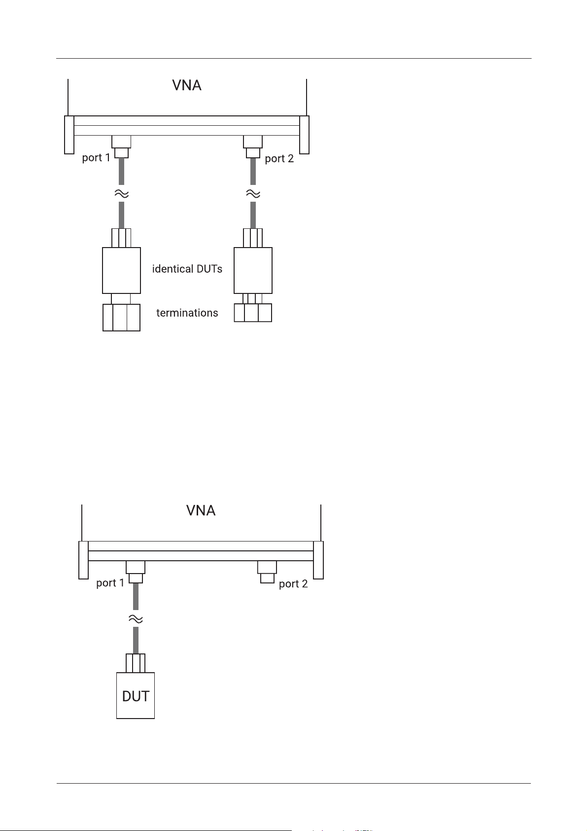
Operation44

If two idential DUTs are available, a conventional isolation

calibration ste

can be carried out as shown

6.3 Measurements

6.3.1 Return loss

In order to carry out return loss measurements (S11) the VNA must be calibrated as described before, either

calibration only, both S11 and S21 or 12-term. The device to be tested (DUT) is then connected to Port 1 of

the VNA as indicated in the figure below. If the DUT can only be connected to the VNA using a cable, then the

VNA should be calibrated at the end of the cable for best results.

Connect device under test to Port 1 to carry out S11

measurements.

PicoVNA 106 6 GHz Vector Network Analyzer 45

Displaying the results

The measurement result can be displayed by selecting the S as described in Display setup

. Note that the measured phase is relative to the calibration reference plane as

discussed in Reference plane extension and de-embedding

parameter and an appropriate display graph

. The reference plane can be shifted at any time from the Enhancement window. Note that changes to the reference plane only take place when the instrument is sweeping.

6.3.2 Insertion loss / gain

To carry out insertion loss measurements (S21) the VNA must be calibrated with the test cables in place, either S between Ports 1 and 2 of the VNA as indicated in the figure below.

For best results, the arrangement shown on the right hand side of the figure should be used whenever possible. When using an S

the other hand, when using a 12-term calibration, this will minimize repeatability / cable flexing errors associated with the connecting cables.

calibration only, both S11 and S21 or full 12-term. The device to be tested (DUT) is then connected

calibration this will minimize errors introduced by the load return loss. On

11+S21

Connect DUT between Ports 1 and 2 to carry out S21

measurements. For best results use the arrangement shown on

Displaying the results

The measurement result can be displayed by selecting the S and described in Reference plane extension and de-embedding

parameter and an appropriate display graph

. Note that the measured phase is relative to the calibration reference plane as discussed in that section. The reference plane can be shifted at any time from the Enhancement window. Note that changes to the reference plane only take place when the instrument is sweeping.

6.3.3 Complete 2-port measurement

In order to measure all four s-parameters a 12-term calibration needs to be completed. The arrangement shown on the right hand side of the figure above is likely to yield best results in terms of repeatability by virtue of using only one test cable, reduces the effects of cable flexing.

Displaying the results

The measurement result can be displayed by selecting a different parameter for each of the possible four display graphs, as described in the previous section. Note that the measured phase is relative to the calibration reference plane as discussed in Reference plane extension and de-embedding plane can be shifted (independently for each parameter) at any time from the Enhancement window. Note that changes to the reference plane only take place when the instrument is sweeping.

. The reference

Maximizing dynamic range

Refer to Calibration for best dynamic range – minimizing the effect of crosstalk

for guidance on achieving

the largest dynamic range.

Operation46

6.3.4 Group delay

Group delay is defined as the rate of change of phase with frequency:

In relatively non-dispersive components such as transmission lines, group delay is the transit time through the line. However, some components such as filters can exhibit negative group delays so care is needed when attaching an interpretation to group delay.

The PicoVNA 106 calculates the group delay by dividing the phase change between adjacent sweep points and dividing by the size of the sweep step. It is usual to apply some degree of trace smoothing to remove very rapidly changing perturbations from the trace. Care should be exercised to ensure that genuine sharp group delay variations are not masked by the smoothing.

Displaying the results

Group delay of any S-parameter can be measured. The result can be displayed by selecting the required parameter and group delay graph from the Display window as described in Display setup

6.3.5 Time domain measurements

The time domain facility allows the display of the time domain response of a network under test. For example, time domain reflectometry (TDR) measurements can be made by first carrying out an S

calibration using 1024 sweep points. Similarly, time domain transmission (TDT) measurements can be made by first completing an S

flowcharts below.

calibration using 1024 sweep points. The steps necessary are shown in the

Performing a TDR measurement

PicoVNA 106 6 GHz Vector Network Analyzer 47

Performing a TDT measurement

Note that carrying out time domain measurements requires a lot of mathematical processing and therefore each sweep will be noticeably slower when displaying time domain.

Examples of TDR measurements using the PicoVNA 106

The trace below shows the time domain response of a 50cm, 50 Ω coaxial cable with an open circuit termination. The trace goes to +1 relative to the reference indicating a reflection coefficient of +1 for an open circuit. The window used is rectangular.

Measured 50 cm line terminated in an open circuit.

The trace below is the same as above except that the ringing either side of the transition has been reduced by the use of a fifth order Kaiser–Bessel window. This reduces the ringing but also slows the rise time.

Same as previous figure but using the Kaiser–Bessel window.

Operation48

The type of window, the order of the Kaiser–Bessel window, and the time span over which the signal is displayed can be selected in the TDR options window, shown below.

Time Domain Options window allows measurement setu

Note: To set a time range either starting or ending beyond 161.66ns, use the Enter T1, T2 facility. However, the displayed total time span must be less than 166.66ns.

The plot below shows the same cable terminated with a short circuit. The window is fifth-order Kaiser– Bessel. This time the trace goes to –1 relative to the reference, indicating a reflection coefficient of –1 for the short circuit.

Measured response of 50 cm shorted cable using Kaiser-Bessel fifth-order window

The trace below shows the effect of increasing the order of the Kaiser–Bessel window to 10. The ripple has been completely removed but the slope of the edge has been further reduced.

PicoVNA 106 6 GHz Vector Network Analyzer 49

Measured response of 50cm shorted cable using tenth-order Kaiser-Bessel window.

A more complicated example:

The trace below shows the response of a 30cm, 50 Ω line followed by 30cm of 25Ω line terminated in a short circuit. The window is third order Kaiser–Bessel. The trace shows the multiple reflections from the discontinuity of impedance at the connection between the lines and the short circuit termination.

Measured response of multiple reflections. See text for details.

The last example is the same 50 Ω / 25 Ω cable combination but this time the termination is an open circuit. The response is also displayed over a longer period.

Measured response of multiple reflections. See text for details.

Operation50

Time domain transmission

Time domain transmission (TDT) is similar to the TDR technique except that the transmitted signal is observed. Traditionally, this is accomplished using a step source and a sampling scope, as with the TDR, but the transmitted signal at the output of the network is observed rather than the reflected signal at the input to the network. This technique is useful for measuring the step response or rise time of amplifiers, filters and other networks.

Examples:

Expected responses from simple RC networks

Measured TDT for 100pF series capacitor

Measured TDT for 100pF shunt capacitor

6.3.6 Reverse measurements on two port devices

In order to measure the reverse parameters (S12 and S22), it is necessary to complete a 12-term calibration first (select ‘insertable’ or ‘non-insertable’ DUT on calibration window as shown in Display setup

calibration options measure only forward parameters. After the 12-term calibration is completed, simply select the reverse parameter(s) to be required on any displayed channel and start the measurement.

). The other

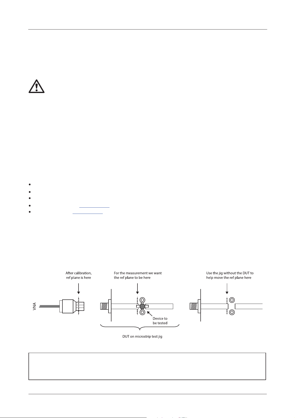
PicoVNA 106 6 GHz Vector Network Analyzer 51

6.3.7 Powering active devices using the built-in bias-Ts

The PicoVNA 106 includes two bias-Ts, which can be used to provide DC bias to the measurement ports 1 and 2. The bias-Ts are rated at 250 mA and can support DC voltages up to 15 V. The DC injection terminals are type SMB, male, and are located on the back panel. This facility can be used, for example, to provide DC bias to an active device being measured.

CAUTION

To avoid causing permanent damage to the internal biasing circuit, do not exceed the voltage and current ratings.

6.4 Reference plane extension and de-embedding

The reference plane extension facility on the PicoVNA 106 allows you to shift the measurement reference plane away from the value set during calibration. This can be useful in removing the effect of interconnecting cables or microstrip lines from measurements. The instrument allows independent reference plane extensions on each of the measurement parameters (S

An example of an application requiring the use of reference plane extension is shown below. In this, it is desired to measure the S

remove the effect of the interconnecting line to the input of the device, the following procedure may be followed:

of a device mounted on a microstrip test jig with SMA connectors. In order to

, S22, S12 or S21).

Perform an S11 calibration at the end of the N to SMA adaptor on Port 1 Connect the test jig without the DUT mounted on it

Display the phase of the S11 on active display channel Click Auto Ref in the Enhancement window

Click Apply in the Enhancement window

The above steps will move the reference plane to the end of the microstrip line. This can be verified by noting that the displayed phase is close to 0° over the entire measurement band. Imperfections associated with the microstrip line and coaxial connector, such as loss and dispersion, will mean that some residual phase will remain. However, with careful design and employing good RF practice for the construction of the jig, this error should remain small.

After the above steps are completed, the DUT can be mounted on the jig and its S

parameter measured.

Example of S11 measurement requiring reference plane extension

Note: The reference plane extension moves the reference plane for each parameter measurement independently. So, if required for example, different values can be used for S

extension value entered, applies to the active channel measurement parameter (either reflection or transmission).

and S21. A reference plane

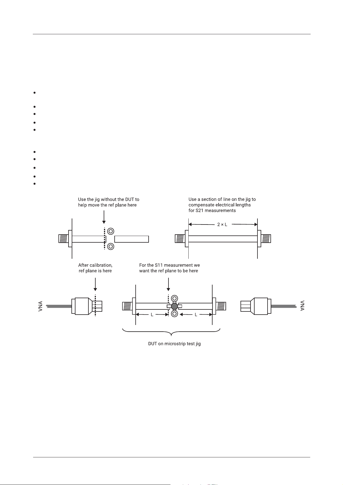
Operation52

In the example above, correction was applied to the S11 phase but not S21. An often-used way to correct the

phase is by using a calibration jig with length of microstrip line equal to the sum of the two sections of

line used either side of the DUT jig (see figure below). Proceed as follows to make S

and S

measurements of the DUT.

Reference plane extension for S

correction

Perform a 12 term calibration (exclude test jig). Ensure that the test cable has connectors of different sex at each end. Adaptors may be needed to connect the DUT. Connect the input port of the test jig without the DUT mounted on it to Port 1 Display the phase of the S11 on the active display channel

Click Auto Ref in the Enhancement window Click Apply in the Enhancement window

Normalization for S

correction

Connect the through microstrip test line between Ports 1 and 2 of the VNA Display the phase of S21 on a non-active channel (keep active channel for S11)

Start the measurement and store data on the S21 channel only to memory (use the memory window) Select Data / Memory for the math function in the Memory window

Select the Memory Math display in the main window

Correcting S21 and S11 phase measurements. Reference plane extension corrects S11 measurements and

normalization to a test line corrects S21.

The above steps will allow the DUT's S

and S21 (or S22 and S12) parameters to be measured with the right

phase correction. In addition, the loss of the microstrip line will be accounted for. The same approach can be used to measure S

and S22. Note, however, that there will be an error on both measurements due to the

imperfections of the microstrip line and connector interface. With careful design of the jig these can be kept acceptably small but further accuracy can be achieved by making use of the de-embedding facility described below.

PicoVNA 106 6 GHz Vector Network Analyzer 53

De-embedding facility

A typical measurement jig, as shown below, includes input and output networks which introduce errors to the measured values of the device under test (DUT). For best measurement accuracy, these networks can be specified (in the form of 2 port s-parameter files) and then used to extrapolate the DUT’s characteristics.

De-embedding allows the effects of the test jig’s input and output networks to be

removed.

The PicoVNA 106 allows you to specify S-parameter files (must be full 2-port data) for the input and output networks as shown in the figure above so that the de-embedding takes place automatically as the instrument measures the test jig. After first calibrating as usual, follow the steps below to enable deembedding.

1. Select the S-parameter file(s) that represent the embedding network(s) by clicking on the embedding

network check box(es) as shown in Measurement enhancement the input network as shown in the figures in Reference plane extension and de-embedding

. Check box Port 1 Network represents

, and Port 2 Network represents the output network. The files selected must be full 2-port S-parameter files in Touchstone format.

2. Click on the radio button in the Measurement enhancement

window to enable de-embedding.

Once the above steps are completed, starting the measurement will display de-embedded results.

The de-embedding facility relies on S-parameter data for the input or output network (or both) being available. This data must be in the form of 2-port S-parameter files in Touchstone format.

Operation54

6.5 Saving data

Measured data can be saved to a file by selecting File > Save Measurements in the main menu. Various formats are available as shown. In all cases, frequency is saved in megahertz. Note that only the

Touchstone format can later be read back into the instrument’s memory trace.

The Save Measurements window is used to save data

Note: For true compatibility with the Touchstone format, only 1-port or full 2-port S-parameters should be saved. For example, selecting S

If required, the data can be saved with the memory math function applied as described earlier under Memory

facility. In order to do this, check the Apply Memory Math box. Note that the memory math display function

on the main window

When saving data in Touchstone format, ensure that you provide the file name extension when entering the file name. Typically, for 1-port networks, the extension “.s1p” is used and “.s2p” for 2-port networks. This will help when reading back the data files since, by default, only files with these extensions will be displayed.

Note: Data will be saved with any system Z0 conversion applied.

must be set otherwise the Apply Memory Math check box will be disabled.

and S21 (but not S12 and S22) is not Touchstone compliant.

6.6 Loading data

Measured data (or data from a circuit simulator) can be read into the instrument’s memory trace(s). This can be done by selecting File > Load Measurement in the main menu. The file containing the data (in Touchstone) format is selected by clicking Select Data File.

The data will be read from the file and copied to the appropriate display channel(s). So, for example, assume you read a data file holding full 2-port data. Further, you have only two channels on display showing, say, S

and S21, so only the S11 and S21 data from the data file read will be copied to the memory traces of the displayed channels. Note: system impedance conversion will apply if turned on in the Measurement

enhancement window.

PicoVNA 106 6 GHz Vector Network Analyzer 55

Loading data is done with the File > Load

Measurement menu command

6.7 Plotting graphics

You can plot the graphics displayed on the main window using the File menu. A printer set-up window will appear from you can choose the desired printer and set its properties. If required, you can add a label to the plotted graphics by clicking File > Print / Save Graphics Label.

A label can be added when plotting or saving graphics

A similar plotting facility exists on the P1dB

and AM to PM utilities' control windows.

6.8 Saving graphics

The graphics shown on the main window can be saved in .bmp, .png, .gif, .tif or .jpg formats. This allows measurement results to be directly pasted into most electronic documents. The facility to save the graphics can be found under the main File menu. After clicking, a dialog box will appear allowing you to select the name of the file, its location and format from a drop-down box. As described in the previous section, a label can be added by clicking File > Print / Save Graphics Label.

The save graphics facility is not available on the P1dB can be captured by pressing the Alt+PrtScn key combination. The image can then be pasted to the chosen document from the Edit menu.

and AM to PM utilities. Instead, the graphics on these

Operation56

6.9 Signal generator utility

This utility allows the instrument to act as a simple signal generator with variable output power. The VNA measurement sweep must be stopped first and the control window, shown below, called from the Utilities menu:

The Signal Generator utility control window

6.10 Output power at the 1 dB gain compression point utility

This utility allows the measurement of the power output at the 1 dB gain compression point (P devices such as amplifiers. The measurement can be done at a single frequency or over the entire frequency

plan specified at the last S-parameter measurement calibration. Start the utility from the Utilities menu in the main window.

calibration

1dB

Calibration minimizes errors by removing small variations associated with the instrument’s hardware. The procedure is simple, as shown below.

Ensure that an S21 (or S11 + S21, or 12-term) calibration has been carried out Connect Port 1 to Port 2 as shown on the left-hand side of the figure below

Enter Input Attenuation and Output Attenuation values (or select Read from file) Enter the test frequency (or select Use sweep plan) and click Calibrate

test

1dB

The basic connection arrangement is shown on the right hand side of the figure below. Note that the input and output attenuators should be carefully selected to ensure that the DUT compresses whilst preventing the power at Port 2 of the instrument exceeding the nominal limit of +10 dBm. It is recommended that the following guidelines are used to estimate the value of the input and output attenuators needed.

1dB(DUT)

– G

(DUT)

–1 + A

= –5 ± 2 dBm

tt1

) of active

1dB

where: P

1dB(DUT)

(DUT)

tt1

= output power of DUT at the 1 dB gain compression point

= linear gain of DUT

, A

= input and output attenuators

tt2

1dB(DUT)

– A

+ 5 < 10 dBm

tt2

PicoVNA 106 6 GHz Vector Network Analyzer 57

Basic connection guide for P1dB measurements. Calibration connection is shown on the left.

The instrument makes the measurement by setting the signal source (Port 1) frequency to the chosen value and then stepping its power from –20 to 0dBm in 1 dB steps. The gain at each power setting is recorded. On completion of the power sweep, a second order curve is fitted over a narrow section centered on the point closest to the 1 dB gain compression point. The coefficients of this curve allow the actual P

point to

1dB

be calculated.

Note: Choose the input attenuator with care. Ensure that there is no gain compression at the start of the power sweep (–20 dBm at Port 1) and that at least 0.7 dB of gain compression is reached at the end of the sweep (0 dBm at Port 1). A ‘?’ will be displayed if insufficient compression has been achieved.

After the attenuator values have been established and the DUT is in place (and powered up as appropriate), enter the values into the P

directly on the P

value, it is important to enter an accurate value that takes into account all losses in the

1dB

control window (Fig. 6.34). Note that the output attenuation value impacts

1dB

output path, including any connecting cable that may have been used.

Clicking Start will perform the test, plot the gain and output power curves, and compute the P

1dB

. This,

together with the linear gain, will be displayed in the text boxes to the right of the Start button. The results can then be printed (the window as displayed will be printed) or saved as a text file by clicking Print or Save.

Operation58

The P1dB measurement utility control window

Attenuation values from file

When measuring P values from a file. The data is held in a simple text file with one line for each frequency point. The format

must be as follows:

using the frequency sweep plan, it is possible to read the input and output attenuation

1dB

Frequency (MHz), magnitude (dB), phase (degrees)

Note: The number of lines in the file must match the number of sweep points in the sweep plan.

6.11 AM to PM conversion utility

This utility allows the measurement of the AM to PM conversion factor of a DUT. Generally it is used for evaluating the linearity of active devices such as amplifiers. The utility is started from the main Utilities menu, shown below:

Figure: The AM to PM measurement utility control window

PicoVNA 106 6 GHz Vector Network Analyzer 59

In order to use this facility an S21 calibration (or S11+S21, or 12-term) must have been carried out. For best results, some averaging (e.g. 16) should be used. Further, a second through calibration is suggested to

remove residual phase variations. The steps are summarized as follows.

AM to PM utility (calibration)

Perform a normal S21 calibration (or S11+S21, or 12-term); see left-hand connection diagram in Quick start

guide

Call up AM to PM Utility (window shown above) Enter frequency required (Test Freq) in megahertz Click Calibrate (connection as on left-hand side of figure below)

AM to PM utility (test)

Connect DUT with attenuators as shown on right hand side of the figure below Enter attenuator values, input power at which result is required and measurement title Power up DUT if necessary Click Start

On completion of the AM to PM test, a graph of AM to PM as a function of input power at the DUT input will be plotted. In addition, the AM to PM factor at the specified input power entered will be displayed in the text box in the Measure section of the window.

Figure: Calibration (left) and test connections for AM to PM test

Note: For best AM-PM results apply some averaging (e.g. 16) and carry out an AM-PM calibration (left hand side of figure). A ‘?’ will displayed if the requested P

for readout is outside the available range.

6.12 Compare data utility

The compare data utility provides a quick and simple way to compare two sets of full S-parameter measurements taking into account the instrument’s measurement uncertainty and optionally, the uncertainty associated with the reference measurement. Typically this facility can be used to measure a verification (reference) DUT and compare the measurement values produced by the PicoVNA 106 VNA with those supplied with the verification DUT. This is a simple and quick way of determining the adequacy of the calibration and calibration kit to be used.

The compare data utility can be found in the utility drop-down menu. This brings up the dialog shown below.

For the compare utility to work, you need to follow these steps:

Perform a full S-parameter calibration Measure the reference DUT

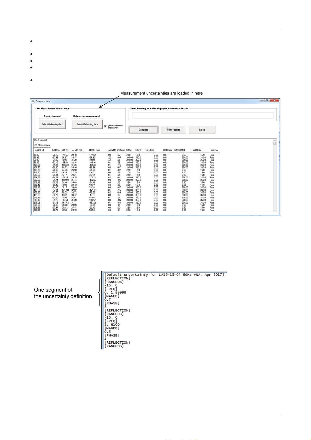
Operation60

Load the reference measurement of the DUT (supplied with the DUT) using Load Measurement (this must be a full s-parameter measurement) Launch the compare data utility Load the PicoVNA 106 VNA uncertainty file (usually in the file DefUnc.dat) Load the reference measurement uncertainty file (this may be ignored in most cases where reference measurements are believed to be highly accurate) Click on the ‘Compare’ button to perform the comparison and display the results

Data comparison dialo

Defining uncertainties

Measurement uncertainty is defined by means of text file as illustrated below. The definition is made up of several segments. Each segment refers to reflection [REFLECTION] or transmission [TRANSMISSION] with an entry for the applicable range in dB followed by the frequency range (in MHz). After the frequency range entry, the magnitude uncertainty in dB is specified followed by the corresponding phase uncertainty in degrees.

The uncertainty definition is made up of several reflection and transmission

ments. A reflection segment is highlighted above.

It is possible to define the uncertainty by a polynomial. To do this, follow the [MAGDB] keyword with the keyword [POLY]. Then, the uncertainty can be define by means of 3 coefficients, say, K

, K1, and K2. The

uncertainty for given measured absolute magnitude value in dB, M, is given by:

= K0 + K1M + K2M

PicoVNA 106 6 GHz Vector Network Analyzer 61

The same approach can be used to defining the phase uncertainty. That is, add the keyword [POLY] after the [PHASE] keyword.

The data compare utility resolves the total combined uncertainty as follows:

In the above, UI is the uncertainty associated with the PicoVNA 106 VNA and UR is that provided with the reference DUT.

6.13 Closing down the software

It is recommended that a formal shut down of the user interface window is carried out before the VNA is to be switched off. This allows the calibration and status to be saved and the instrument’s log file to be updated. The sequence is shown below:

Formally closing down the software saves the current calibration

Performance verification and maintenance62

7 Performance verification and maintenance

It is recommended that the instrument is checked annually for safety (chassis grounding, fan operation, clear ventilation grilles and operator markings) and compliance with the stated electrical specification. The table below shows the parameters that should be checked as part of the calibration process. Note that the ventilation inlets should be checked as described later.

Measurement DUT Conditions Calibration type

S21 and S12, magnitude and phase

S11 and S22, magnitude and phase

or S11, S21, S22 and S12,

magnitude and phase

Table: Suggested annual instrument verification / calibration schedule

20 dB attenuator 51 points sweep

0.3–6000 MHz 1kHz BW +3 dBm test level

A known mismatch at ports 1 and 2 (–16 dB or worse return loss)

Mismatched attenuator (> 10 dB attenuation and –16 dB or worse return loss)

51 points sweep

0.3–6000 MHz 1kHz BW +3 dBm test level

51 points sweep

0.3–6000 MHz 1kHz BW +3 dBm test level

12 term

We recommended that you compare the measured results with the values provided with the standards and verify that they are within the combined uncertainty of the instrument and the provided measurements. The frequency should be set to agree with those available(s) for the standard used. The recommended test arrangement is shown below. The results should be within the instrument’s quoted uncertainty as detailed in the following section. Allowance should also be made for the uncertainty of the standard reference values.

Figure: Performance verification arrangement

Tip: A data compare utility is provided in the PicoVNA 2 software that can be used to compare the measurements, taking into account the uncertainty of the instrument.

7.1 Measurement uncertainty

The measurement uncertainty figures below are based on calibration (12 term, insertable device, with –3 dBm test power and using 10 Hz bandwidth) using the premium PC3.5 mm calibration kits optionally supplied with the instrument. The figures for S

less than 0.2. Similarly, the figures for S

and S22 assume the DUT has a value of S21 or S12 of less than 0.2.

and S12 assume that the DUT has a value of S11 or S22 of

Other external factors such as connector and cables effects are excluded.

PicoVNA 106 6 GHz Vector Network Analyzer 63

Power Frequency Magnitude Phase

–15 dB to 0 dB Freq < 2 MHz

Freq > 2 MHz

–25 dB to –15 dB Freq < 2 MHz

Freq > 2MHz

–30 dB to –25 dB Freq < 2MHz

Freq > 2MHz

0.7

0.5

0.8

1.0

3.0

2.5

8º 4º

10º

6º

20º 15º

Table: Reflection (S11, S22) measurement uncertainty

Power Frequency Magnitude Phase

+0 dBm to +6 dBm Freq < 2 MHz

Freq > 2 MHz

–40 dBm to 0 dBm Freq < 2 MHz

Freq > 2 MHz

–60 dBm to –40 dBm Freq < 2 MHz

Freq > 2 MHz

–80 dBm to –60 dBm Freq < 2 MHz

Freq > 2 MHz

0.4

0.2

0.3

0.1

0.5

0.3

2.0

1.5

6º 2º

2º 1º

8º 4º

15º 12º

Table: Transmission (S21, S12) measurement uncertainty

7.2 Routine maintenance

Ventilation grilles

Check that all ventilation grilles are clear of any debris, dust or any other material that may impede the flow of air. Particularly, check the vents in the bottom panel of the instrument. It is advisable to brush these to remove any gradual build up of dust.

Failure to clean the ventilation grilles may lead to overheating and eventual failure of the instrument.

Front panel connectors

Routinely inspect the Port 1 and Port 2 N-type connectors for signs of damage or dirt. Use connector-saver adaptors (male to female through) where frequent connection and disconnection are likely.

Performance specification64

8 Performance specification

The instrument’s performance specification is given below. Unless otherwise stated, the figures apply with 10 Hz resolution bandwidth, at –3 dBm test power, at an ambient temperature of 23 ± 1°C and 60minutes after power up.

Measuring functions

Measuring parameters S11, S21, S22, S

(power at 1 dB gain compression)

1dB

AM-PM conversion factor

Error correction 12 term

8 term (unknown through calibration) S

(1 port correction)

(normalize, normalize + isolation)

(source match correction + normalize + isolation)

Averaging, smoothing, Hann and Kaiser–Bessel filtering on time-domain measurements, Electrical length compensation (manual) Electrical length compensation (auto) De-embed (2 embedding networks may be specified)

Impedance conversion Display channels 4 channels (CH1, CH2, CH3, CH4) Traces 2 traces / channel Display formats Amplitude (logarithmic and linear), phase, group

delay, VSWR, real, imaginary, Smith chart, polar, time

domain Memory trace One per channel Limit lines 6 segments per channel (overlap allowed) Markers 8 markers Marker functions Normal, ∆ marker, fixed marker, peak / min, 3 dB and

6 dB bandwidth

Signal source characteristics

Frequency range 300 kHz to 6.02 GHz Frequency setting resolution 10 Hz Frequency accuracy ±10 ppm (23 ± 3°C) Frequency temperature stability ±0.5 ppm/°C (15 to 35°C) Harmonics (–3 dBm output level) –20 dBc Non-harmonic spurious (typical) –40 dBc Phase noise (10 kHz) –90 dBc/Hz (0.3 MHz to 1000 MHz)

–80 dBc/Hz (1000 MHz to 4000 MHz)

–76 dBc/Hz (> 4000 MHz) Output power +6 to –20 dBm (+3 to –20 dBm for F > 4GHz) Power setting resolution 0.1 dB (nominal) Output power accuracy ±2.0 dB Reference input frequency 10 MHz ±6 ppm Reference input level 0 ±3 dBm Reference output level 0 ±3 dBm

Sweep functions

Sweep type Linear sweep, CW sweep (timed sweep)

PicoVNA 106 6 GHz Vector Network Analyzer 65

Sweep functions

Power sweep (P

1dB

utility)

Trigger modes Free run

Positive trigger

Negative trigger

Manual trigger Sweep time (full 2-port calibration, 20 kHz bandwidth,

201 points: 37 ms no averaging)

Number of points 51, 101, 201, 401, 801, 1001, 1024, 2001, 4001, 9001,

10 001

Receiver characteristics

Resolution bandwidth 140 kHz, 70 kHz, 35 kHz, 15 kHz, 10 kHz, 5 kHz, 1

kHz, 500Hz, 100Hz, 50Hz, 10Hz

Averaged displayed noise floor (dB): S

calibration

10 Hz bandwidth 16 averages Test ports terminated as during isolation calibration step

Dynamic range (dB)

Band Typ Max

0.3 MHz to 10 MHz –110 –100

10 MHz to 4 GHz –118 –108

4 GHz to 6 GHz –110 –100

See figure below Bandwidth 20Hz 16 averages Test ports terminated as during the isolation calibration step. Isolation calibration refreshed as described in 6.2.7.

Temperature stability (typical) 0.02 dB/°C (f < 4 GHz)

0.04 dB/°C (f ≥ 4 GHz)

Trace noise (mdB RMS) Full band Test level 0dB 201 point sweep

Bandwidth Typ Max

10 kHz 0.8 2

70 kHz 3 5

140 kHz 5 10

Test port characteristics

Load match (uncorrected) 16 dB typ. Source match (uncorrected) 16 dB typ (uncorrected)

40 dB min (48 dB typical) Directivity (corrected, using PC3.5 cal kit) 40 dB min (47 dB typical) Crosstalk (dB, corrected)

Test ports terminated with short circuits. Value is average displayed noise level.

Band Typ Max

0.3kHz–2MHz –110 –90

2 MHz–4 GHz –110 –90

4 GHz–6 GHz –100 –90 Main test ports maximum input level

+10 dBm (1 dB compression)

Main test ports maximum input level

+20 dBm (no damage)

Main test ports connectors Type N (female) Bias-T maximum current 250 mA Bias-T maximum DC voltage +15 V Bias-T current protection Built-in resettable fuse Bias-T DC port connectors SMB (female on front panel) Sweep trigger input voltage Low: –0.1 to +1.0 V

Performance specification66

Test port characteristics

High: +2.0 to +4 V

P1dB utility

Frequency range 0.3 to 6020 MHz Input power sweep range –20 to 0 dBm Input power sweep step 1 dB (nominal) P1dB calculation method

2nd order curve fit Display format Graphical, gain and output power Accuracy 0.5 dB (typical)

AM to PM utility

Frequency range 0.3 to 6020 MHz Input power sweep range –20 to 0 dBm Input power sweep step 1 dB (nominal) AM to PM point calculation method

2nd order curve fit Display format Graphical, phase conversion (deg / dB) Accuracy (Port 2 power +5 to –20 dBm) 1° (typical)

Signal generator utility

Frequency range 0.3 to 6020 MHz Output power –20 to +3 dBm Setting resolution 0.1 dB Output power accuracy +2.0 dB max

Group delay

Range (180° maximum phase shift per frequency step)

where ∆f is the aperture frequency Aperture frequency Frequency sweep step size Accuracy

Data handling

Calibration data Store / Recall on disk Calibration kit data Store / Recall on disk Print measured data (graphics) To any printer installed on host PC Save measured data (graphics) To disk Measured data Store on disk Measured data (Touchstone format) Store on disk Measured data (Touchstone format) Recall to memory trace from disk

Statement of Volatility: No user data, calibration data or user settings are stored on the device.

Miscellaneous

PC data interface USB PC minimum requirements Pentium 4 (3 GHz) or equivalent

1 GB RAM

200 MB hard disk storage on C: partition

Windows 7, 8 or 10

Display resolution of 1280 x 720 External dimensions (L x W x H) 286 x 174 x 61 mm Weight 1.85 kg

PicoVNA 106 6 GHz Vector Network Analyzer 67

Miscellaneous

Temperature range (operating) 15 °C to 35 °C Temperature range (storage) –20 °C to 50 °C Humidity 80% max. (non-condensing) Power source DC, 12 to 15 V, 1.85 A max.

Figures: Typical system dynamic range (P

Dynamic range 10 MHz to 6 GHz

Dynamic range 0.3 to 10 MHz

= +6 dBm, BW = 10 Hz)

test

9 Troubleshooting guide

CAUTION

Symptom Possible Cause Solution

Instrument does not power up

PicoVNA 2 software unable to communicate with the instrument

Instrument sweeping but display not refreshing

‘Last Calibration not found’ message on power up

Diagnostics Tests (under Tools menu) fail

Error reading data files

Power not applied Incorrect supply

Driver not installed Link interrupted

Data link interrupted Restart instrument and software

C: \User\Public\Documents\PicoVNA 2 directory deleted or corrupted

Data corruption Restart instrument and software.

Invalid format Too many lines Leading space(s)

Check DC connection Check external supply

See Switching on Restart instrument and software

Restore folder. Set up display and calibrate. Exit the software using File > Exit menu command. This will save the current calibration in a file named

defaultcal.cal.

Ensure that test cable used is in good condition.

Check for correct format / ‘#’ line Number of lines must be < 1000 Remove leading spaces from data lines

Troubleshooting guide68

Diagnostics tests

It is possible to run self-check tests on the instrument. This facility (Diagnostic Tests) is available from the Tools menu shown above. In order to complete the tests a low loss cable is required to link Port 1 to Port 2. The tests carry out the following checks.

Synthesizers: test that they remain in lock over the frequency range Test signal: test the level range and step size Receiver levels: test that the receiver is operating at normal signal levels Receiver crosstalk: test that raw crosstalk remains below limit Receiver DC offset: test that this is at normal level

PicoVNA 106 6 GHz Vector Network Analyzer 69

Figure: The Diagnostics Tests perform internal checks on key components

If any of the tests returns an error, check connectors and linking cable. If this does not resolve it, restart the instrument and the software. After pressing reset, wait until the front-panel channel activity indicators have stopped flashing to continue with the tests.

Calibration error terms and raw receiver data

The diagnostic tests dialog (figure above) also provides the facility for retrieving the calibration error terms and raw receiver data. The latter can be helpful for users wishing to carry out their own calibration procedure.

Back up/restore EEPROM

This facility allows the internal ROM (read-only memory) of the instrument to be backed up or restored. This facility should only be required by service or repair personnel.

Warranty70

10 Warranty

Pico Technology warrants upon delivery, and for a period of three years unless otherwise stated from the date of delivery, that the Goods will be free from defects in material and workmanship.

Pico Technology shall not be liable for a breach of the warranty if the defect has been caused by fair wear and tear, willful damage, negligence, abnormal working conditions or failure to follow Pico Technology's spoken or written advice on the storage, installation, commissioning, use or maintenance of the Goods or (if no advice has been given) good trade practice; or if the Customer alters or repairs such Goods without the written consent of Pico Technology.

PicoVNA 106 6 GHz Vector Network Analyzer 71

Index

2-port measurement, complete 45

Altitude 3 AM to PM conversion measurement 58

Bias-tees 51

Calibration 4, 14, 38 Calibration for best dynamic range – minimizing the effect

of crosstalk 43 Calibration kit parameters 23

Calibration steps for all s-parameters measurements (insertable DUT) 42

Calibration steps for all s-parameters measurements (non-insertable DUT) 42

Calibration steps for S11 and S21 measurements 41 Calibration steps for S11 measurements 41 Calibration steps for S21 measurements 41 Closing the software 61

Humidity 3

Insertion loss/gain measurement 45 Installing the software 22 Introduction 10

Limit lines facility 35 Loading data 54

Main window 27 Maintenance

for performance 62 for safety 63

Matched termination with poor return loss or unmodeled Short and Open 25

Measurement 11 Measurement enhancement 31 Measurement start/stop 37 Measurement uncertainty 62 Memory facility 34 Minimum requirements 22

Data markers 29 De-embedding 51 Description 8 Display setup 27 Displaying measurements 14

Environment 3 Error correction 14 Error messages 22

Frequency sweep settings, changing 40

Getting started 22 Grounding 2 Group delay measurement 46

Operation 27 Output power at the 1 dB gain compression point utility

PC data link interruption 37 Performance verification 62 Plotting graphics 55 Pollution degree 3 Power connection 3

Ranges, maximum 1 Reference plane extension 51 Repair 4 Return loss 44 Reverse measurements on two-port devices 50

Safety

introduction 1

symbols 1 Saving data 54 Saving graphics 55 Servicing 4 Signal generator utility 56 S-parameters 11 Specifications 64 Status panel 36 Structure of the VNA 10 Sweep trigger output 37 Switching on the VNA 23

TDR

bandpass method 20

lowpass method 20 Temperature 3 Time domain measurements 46 Triggered sweep 37 Troubleshooting guide 68

Index72

USB connection 3

Warranty 70

USA headquartersUK headquarters

Asia-Pacific head office:

Pico Technology James House Colmworth Business Park St. Neots Cambridgeshire PE19 8YP

Distribution in the UK & Ireland

United Kingdom

Tel: +44 (0) 1480 396 395 Fax: +44 (0) 1480 396 296

Characterisation, Measurement & Analysis

sales@picotech.com

support@picotech.com

Pico Technology 320 N Glenwood Blvd Tyler Texas 75702 United States

Lambda Photometrics Limited

Lambda House Batford Mill Harpenden Herts AL5 5BZ United Kingdom

E: info@lambdaphoto.co.uk W: www.lambdaphoto.co.uk T: +44 (0)1582 764334

F: +44 (0)1582 712084

Tel: +1 800 591 2796 Fax: +1 620 272 0981

www.picotech.com

Pico Technology Room 2252, 22/F, Centro 568 Hengfeng Road Zhabei District Shanghai 200070 PR China

Tel: +86 21 2226-5152

pico.china@picotech.com

PICO PicoVNA 106 User Manual

Specifications and Main Features

Frequently Asked Questions

User Manual